Embed Size (px)
Citation preview

Shale Gas and Emerging Market Dynamics
The Rice World Gas Trade Model:The Impact of the Shale Resource
Kenneth B Medlock IIIJames A Baker III and Susan G Baker Fellow in Energy and Resource Economics,
James A Baker III Institute for Public PolicyAdjunct Professor, Department of Economics
Peter R HartleyGeorge and Cynthia Mitchell Professor of Economics, Department of Economics
Rice Scholar, James A Baker III Institute for Public Policy
October 15, 2010
James A Baker III Institute for Public PolicyRice University

A Paradigm Shift• The view of natural gas has changed dramatically in only 10 years
– Most predictions were for a dramatic increase in LNG imports to North America and Europe.
– Today, growth opportunities for LNG developers are seen in primarily in Asia.
• Many investments were made to expand LNG potential to North America in particular
– At one point, 47 terminals were in the permitting phase.
– Since 2000, 2 terminals were re-commissioned and expanded (Cove Point and Elba); 9 others were constructed.
– In 2000, import capacity was just over 2 bcfd; It now stands at just over 17.4 bcfd.
– By 2012, it could reach 20 bcfd.
• A similar story in Europe– In 2000, capacity was just over 7
bcfd; It is now over 14.5 bcfd.
– By 2012, it could exceed 17 bcfd.
• Shale gas developments have since turned expectations upside-down

Shale is not confined to North America, and it has significant implications for the global gas market
Major North American Shale Plays
Other Shale Plays
(Limited data available publicly)

The Global Shale Gas Resource• Knowledge of shale gas resource is not new
– Rogner (1997) estimated over 16,000 tcf of shale gas resource in-place globally
– Only a very small fraction (<10%) of this was deemed to be technically recoverable and even less so economically.
• Only recently have innovations made this resource accessible
– Shale developments have been focused largely in North America where high prices have encouraged cost-reducing innovations.
– IEA recently estimated about 40% of the estimates resource in-place by Rogner (1997) will ultimately be technically recoverable.
– Recent assessment by Advanced Resources International (2010) notes a greater resource in-place estimate than Rogner (1997), with most of the addition coming in North America and Europe.
• We learn as we advance in this play!
Region
Resource In-Place (tcf)
Resource In-Place (tcm)
North America 3,842 109
Latin America 2,117 60
Europe 549 15
Former USSR 627 18
China and India 3,528 100
Australasia 2,313 66
MENA 2,548 72
Other 588 17
Total 16,112 457
Rogner (1997)

“Resource” vs. “Reserve”• Often, the press and many industry analysts characterize the recent
estimates of shale gas in North America as “reserves”.
• This is an incorrect representation! It is important to understand what these assessments are actually estimating.
• With shale gas, GIP numbers are very large. The X-factor is cost.
Resource in Place
Resource endowment. Lots of uncertainty, but we can never get beyond this ultimate number.
Technically Recoverable Resource
This is the number that is being assessed. Lots of uncertainty, but experience has shown this number generally grows over time.
Economically Recoverable Resource
This will grow with decreasing costs and rising prices, but is bound by technology.
Proved Reserves
Connected and ready to produce.

A Comment on Development Costs• “Breakeven cost” is often discussed, but it is important to put this into context…
• The cost environment is critical to understanding what prices will be. For example, F&D costs in the 1990s yield long run prices in the $3-$4 range.
• What will the cost of steel and cement be? What about field services?
0
50
100
150
200
250
300
1980
1981
1982
1983
1984
1985
1986
1987
1988
1989
1990
1991
1992
1993
1994
1995
1996
1997
1998
1999
2000
2001
2002
2003
2004
2005
2006
2007
2008
2009
Real Well Cost KLEMS Real Oil Price
Index2000=100
Real cost going forward is roughly equal to costs in
1982, 2004/05, 2009

North American Shale Gas
• In 2003, NPC estimate of placed the resource at 38 tcf.
• In 2005, EIA estimate placed the resource at about 140 tcf.
• Recent estimates are much higher
– (2008) Navigant Consulting, Inc. estimated a mean of about 620 tcf, with a low of 348 tcf and a high of 892 tcf.
– (2009) PGC reports over 680 tcf.
– (2010) ARI estimates over 1000 tcf.
• Bottom Line:
• Resource assessment is large. Our work at BIPP indicates a technically recoverable resource of 669 tcf.
• We learn more as time passes!
Mean Technically Recoverable Resource (tcf) Breakeven Price
Antrim 13.2 5.50$ Devonian/Ohio 170.8
Utica 5.4 6.50$ Marcellus 135.4
Marcellus T1 47.4 4.50$ Marcellus T2 43.3 5.25$ Marcellus T3 44.7 6.50$
NW Ohio 2.7 7.00$ Devonian Siltstone and Shale 1.3 7.00$ Catskill Sandstones 11.7 7.00$ Berea Sandstones 6.8 7.00$ Big Sandy (Huron) 6.3 6.00$ Nora/Haysi (Huron) 1.2 6.50$
New Albany 3.8 7.25$ Floyd/Chatanooga 2.1 6.00$ Haynesville 105.0
Haynesville T1 42.0 4.25$ Haynesville T2 36.8 5.00$ Haynesville T3 26.3 6.25$
Fayetteville 36.0 5.00$ Woodford Arkoma 8.0 5.50$ Woodford Ardmore 4.2 6.00$ Barnett 54.0
Barnett T1 32.2 4.50$ Barnett T2 21.8 5.75$
Barnett and Woodford 35.4 7.00$ Eagle Ford 20.0 4.25$ Palo Duro 4.7 7.00$ Lewis 10.2 7.00$ Bakken 1.8 6.50$ Niobrara (incl. Wattenburg) 1.3 7.00$ Hilliard/Baxter/Mancos 11.8 7.00$ Lewis 13.5 7.00$ Mowry 8.5 7.00$
Montney 65.0 4.75$ Horn River 90.0 5.00$ Utica 10.0 6.50$
Total US Shale 504.2Total Canadian Shale 165.0Total North America 669.2

North American Shale Gas (cont.)
• Shale is distributed in many locations, some traditional producing areas but others are in the heart of market areas.
• Supply potential in BC, in particular, has pushed the idea of LNG exports targeting the Asian market
– Asia is an oil-indexed market.– Competing projects include
pipelines from Russia and the Caspian States, as well as LNG from other locations.
– BC is a basis disadvantaged market, but selling to Asia could provide much more value to developers.
• For those regions not accustomed to seeing robust natural gas development, regulatory conflicts are being realized.
Horn River
Montney

The North American Resource Base
• North American resources are large, but must be placed in a global context. – FSU and Middle East (pictured for comparison) are larger and generally less costly.
However, access and transportation costs make North American resources preferential in the short-to-medium term.
– Cost reductions and higher recoverable resource estimates benefit the US supply picture.

Modeling Results

Henry Hub Natural Gas Price
• Long term prices at Henry Hub (averages, inflation adjusted)– 2010-2020: $ 5.57 2021-2030: $ 6.21 2031-2040: $ 6.98

North American Shale Production
US

Composition of U.S. Production
• US shale production grows to about 50% of total production by 2040.
• Canadian shale production grows to about 1/3 of total output by 2040 (not pictured). This offsets declines in other resources as total production remains fairly flat.

The Impact of European Shale Production
• European shale production grows to about 25% of total production by 2040. While this is not as strong as North America, it does offset the need for increased imports from Russia, North Africa, and LNG. In fact, the impact of shale growth in Europe is tilted toward offsetting Russian imports, but it also lowers North Sea production at the margin, as well as other sources of imports.

LNG Imports targeting the US• Growth in North American shale resources renders load factors very low.
– Load factors approach an average of 35% by the mid-2030s. However, they remain below 20% for the balance of the next two decades.

Regional Pricing
• The spread between Henry Hub and NBP widens (depicted as HH-NBP), which generally favors deliveries to non-US markets

LNG Imports to Europe
• Growth in LNG is an important source of diversification to Europe. Indigenous shale gas opportunities abate this to some extent, but the shale revolution is not as strong as in North America.

LNG Imports to Asia
• Strong demand growth creates a much needed sink for LNG supplies.– China leads in LNG import growth despite growth in pipeline imports and
supplies from domestic unconventional sources.

Global Gas Trade:LNG vs. Pipeline and Market Connectedness
• Globally, LNG growth is strong, reaching about 50% of total international natural gas trade by the early 2030s. Tis is driven largely by demand in Asia.
• Previously disconnected regional markets become linked.

LNG Exports
• Strong growth longer term from Russia, Venezuela and Iran. Growth through the late 2020s is dominated by Qatar and Australia.

Scenario Results:Examining the impact of various policy stimuli

Natural Gas Demand Response• Natural Gas demand is sensitive to the CO2 price and the relative price of
natural gas. A general relationship follows from the scenarios examined in the RWEM.
• Graphic depicts the increase in demand relative to the Reference Case.

Natural Gas Demand Across Scenarios
• Natural Gas demand impulse predicted by the scenario analyses performed in the RWEM.– We focus on a subset of these scenarios.

Natural Gas Demand Across
Scenarios (cont.)
• Demand in the US increases the most with the three scenarios analyzed, although patterns are different.
• The 50X50 with Offsets case sees different trade patterns specifically because the policy effects Europe, Japan, Korea, Australia, New Zealand and Canada as well as the US.
• Demand in Canada is lower when policy only affects US demand.

LNG Imports Across Scenarios
• Annual LNG imports in North America increases with demand.
• In the 50X50 with Offsets case, there is greater competition for LNG as demand in other countries is also higher.
• There are some intertemporal effects as investment patterns change.

Shale Gas Production
Across Scenarios
• Shale gas production in North America also increases.
• There are some intertemporal effects as investment patterns change.
• Regional impacts vary, but the biggest response is seen from the Marcellus shale.

LNG Exports Across
Scenarios
• Some countries are benefitted more than others.
• In particular, as the level of LNG imports in the US increases.
• The 50X50 with Offsets case sees the greatest increase in LNG trade.
• Iran and the Middle East more generally account for the bulk of the increase in exports.

Questions

Appendix

Comments on Gas Market Globalization

Globalization
Hartley and Medlock (2006) demonstrate that local shocks will be transmitted across previously disconnected regional markets more easily as LNG trade expands.
This begs the question, “Will increased LNG trade leave the US increasingly exposed to international market fluctuations?”
If so, we can also ask, “Is globalization welfare improving?”
Hartley and Medlock (2006, 2008, 2009) demonstrates that growth in LNG trade implies growth in physical liquidity, i.e. - supply options are expanded. This provides a means of dealing with unexpected shocks.
Example 1: Europe dealing with a Russian cut-off of supplies
Example 2: Market flexibility in the event of a US hurricane disruption

Globalization (cont.)
Brito and Hartley (2007) also show that growth in physical liquidity also limits the ability of a single supplier to price above marginal cost.
Of course, other important questions are motivated in the context of globalization of gas markets, such as
What is the likelihood of a cartel emerging?
What is the effect of environmental policy aimed at reducing CO2emissions?
or even New Source Performance Standards in the US?
What is the effect of policy that limits access to resources?
What is the effect of the expansion of shale gas production?

The Role of Oil IndexationAbsent storage and physical liquidity, oil indexation provides an element of price certainty. Oil indexation is a form of price discrimination
(1) Firm must be able to distinguish consumers and prevent resale.(2) Different consumers have different elasticity of demand.Both conditions are met in Europe and Asia, but not in North America.
Lack of transport differentials in Europe is evidence of discrimination.
Increased ability to trade between suppliers and consumers (physical liquidity) violates condition (1).
This will happen in a liberalized market or as LNG trade grows.
Evidence of a weaker ability to price discriminate is emerging in
S
D
P@ P=MC
POIL INDEX
Oil Indexed Contract Volume
“Spot” Volume
Total Volume
P
Q
Rent earned from pricing supply above marginal cost
Marginal price

The Role of Shale Gas
Expansion of production from shale plays has rendered the utilization of LNG import capacity in the US very low.
Moreover, Hartley and Medlock (2010) indicate that, in the aggregate, average annual capacity utilization of US LNG regasification terminals may not exceed 20% until the 2030s.
Current and potential future expansion of shale gas in the US, Europe and Asia effectively makes the global natural gas supply curve more elastic.
This mitigates the potential for sustained increases in price.
To the extent that shale gas production is more of a manufacturing process than production from other natural gas plays, the idea of “just-in-time” production could also simulate the traditional role of storage.Thus, shale gas production may also limit seasonal volatility to some extent.

The Rice World Gas Trade Model

The RWGTM• The Rice World Gas Trade Model (RWGTM) has been developed to
examine potential futures for global natural gas, and to quantify the impacts of geopolitical influences on the development of a global natural gas market.
• The model predicts regional prices, regional supplies and demands and inter-regional flows.
• Regions are defined at the country and sub-country level, with extensive representation of transportation infrastructure
• The model is non-stochastic, but it allows analysis of many different scenarios. Geopolitical influences can alter otherwise economic outcomes
• The model is constructed using the MarketBuilder software from Altos
– Dynamic spatial general equilibrium linked through time by Hotelling-type optimization of resource extraction
– Capacity expansion is determined by current and future prices along with capital costs of expansion, operating and maintenance costs of new and existing capacity, and revenues resulting from future outputs and prices.

The RWGTM: Demand• Over 290 regions.
– North America (residential, commercial, power generation and industrial sectors)
• Natural gas demand functions estimated using longitudinal state and provincial data
– Rest of World (Power Gen, Direct Use, EOR)
• Natural gas share of total energy increases with income, reflecting natural gas as a premium fuel, but declines as relative price increases. The price elasticity is decreasing in the natural gas share of TPES. This captures rigidities associated with capital deployment.
• Population growth taken from the UN median case projection to 2050.
• Economic growth is based on conditional convergence.

The RWGTM: Demand (cont.)• Economic growth is based on conditional convergence to historical US
growth rates at various levels of per capita income. The reference path is estimated using a piecewise linear spline regression. Various knots were tested.
-20%
-15%
-10%
-5%
0%
5%
10%
15%
20%
$0 $5,000 $10,000 $15,000 $20,000 $25,000 $30,000 $35,000 $40,000
Per Capita GDP Growth Rate
2.1%
1.2%

The RWGTM: Demand (cont.)• Current economic and financial crisis is incorporated. We use the IMF
outlook for growth through 2014 for all countries. Beyond 2014, growth is governed by a model of conditional convergence. All GDP is in $2005PPP.
China
-2%
0%
2%
4%
6%
8%
10%
12%
14%
16%
1980 1985 1990 1995 2000 2005 2010 2015 2020 2025 2030
forecast
USA
-6%
-4%
-2%
0%
2%
4%
6%
8%
1980 1985 1990 1995 2000 2005 2010 2015 2020 2025 2030
forecast

The RWGTM: Demand (cont.)• International demand: Energy intensity falls as income rises (see Medlock
and Soligo, EJ 2001)– Estimated using dynamic panel regression (70 countries)
• ln(E/Y)t,i = a0,i + a1*ln(Y/POP)t,i + a2*ln(P)t,i + a3*ln(E/Y)t-1,i
• The natural gas share of total energy increases with income, reflecting natural gas as a premium fuel, but declines with relative price increases.
– Dynamic panel regression (29 countries)
– Double log function bounds share between 0 and 1
– Price elasticity is decreasing in the natural gas share of TPES. This captures rigidities associated with capital deployment.
Energy Intensity
0.0000.0050.0100.0150.0200.0250.0300.0350.0400.0450.050
$- $5,000 $10,000 $15,000 $20,000 $25,000 $30,000Per Capita GDP
Energy Demand per Capita
0
50
100
150
200
250
300
350
400
$- $5,000 $10,000 $15,000 $20,000 $25,000 $30,000Per Capita GDP
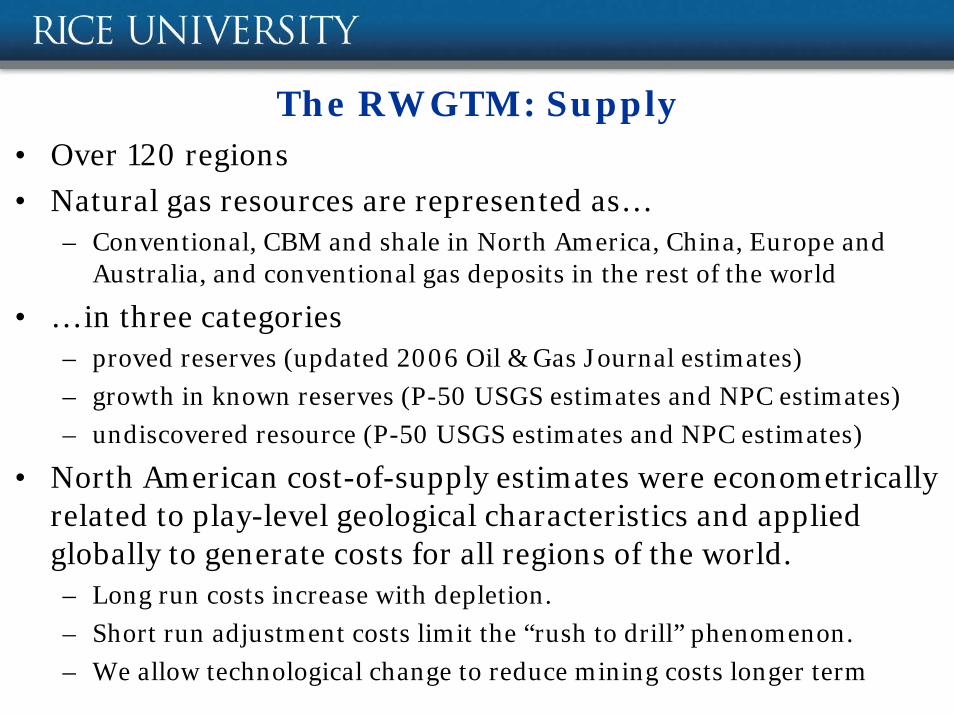
The RWGTM: Supply• Over 120 regions
• Natural gas resources are represented as…– Conventional, CBM and shale in North America, China, Europe and
Australia, and conventional gas deposits in the rest of the world
• … in three categories– proved reserves (updated 2006 Oil & Gas Journal estimates)
– growth in known reserves (P-50 USGS estimates and NPC estimates)
– undiscovered resource (P-50 USGS estimates and NPC estimates)
• North American cost-of-supply estimates were econometrically related to play-level geological characteristics and applied globally to generate costs for all regions of the world. – Long run costs increase with depletion.
– Short run adjustment costs limit the “rush to drill” phenomenon.
– We allow technological change to reduce mining costs longer term

The RWGTM: Supply (cont.)• Selected examples: Regional marginal cost of supply curves…

The RWGTM: Infrastructure• Required return on investment varies by region and type of project (using
ICRG and World Bank data)
• Detailed transportation network
– Pipelines aggregated into corridors where appropriate.
– Capital costs based on analysis of over 100 pipeline projects relating project cost to various factors.
– Tariffs based on posted data, where available, and rate-of-return recovery.
– LNG is represented as a hub-and-spoke network, reflecting the assumption that capacity swaps will occur when profitable.
– LNG shipping rates based on lease rates and voyage time.
• For all capital investments in both the upstream and midstream, we allow for existing and potential pipeline links, then “let the model decide” optimal current and future capacity utilization.
• For detailed information please see Peter Hartley and Kenneth B Medlock III, “The Baker Institute World Gas Trade Model” in The Geopolitics of Natural Gas ed Jaffe Amy David Victor and Mark Hayes Cambridge

The RWGTM: Infrastructure (cont.)• A brief focus on LNG costs
• These are generally generic with regard to region.
Capex ($/mcf) Capex ($/ton)Australia 12.8934 620.2$ Australia (Queensland) 9.0988 437.7$ Atlantic 7.7854 374.5$ Pacific 9.0988 437.7$ Middle East 8.4784 407.8$ Arctic 18.2287 876.8$
Sample Capital Cost for Liquefaction
• A facility must be estimated to earn a return to capital prior to the model choosing to build it.