Send Orders for Reprints to reprints@benthamscience.ae

The Open Petroleum Engineering Journal, 2015, 8, 203-207 203

1874-8341/15 2015 Bentham Open

Open Access Shale Gas Productivity Predicting Model and Analysis of Influence Factors

Yin Daiyin, Wang Dongqi*, Zhang Chengli and Duan Yingjiao

Northeast Petroleum University, Key Laboratory of Enhanced Oil and Gas Recovery of Ministry of Education, Daqing, P.R. China

Abstract: In order to find the dynamic characteristics of shale gas reservoirs and improve shale gas well production, it is very important to research on shale gas seepage mechanism and production evaluation. Based on the shale gas seepage mechanism, adsorption and desorption characteristics, the diffusion mechanism and mass conservation theory in shale gas development, the dual pore medium shale gas reservoir mathematical model is set up. The mathematical model is built by the finite difference method based on start-up pressure gradient, slippage effect and the isothermal adsorption principle, and then programmed to solve it. Finally, this paper analyzed the impact of Langmuir volume, Langmuir pressure, start-up pressure gradient and slippage coefficient and other factors on shale gas wells production.

Keywords: Influence factors, Seepage mechanism, Shale gas, Slippage effect, Start-up pressure gradient.

1. INTRODUCTION

The exploration and development of the shale gas, a kind of unconventional oil and gas resources [1-3], is getting more and more attention in the oil industry. Global shale gas resource is about 456.24×1012m3. Shale gas resources in our China is very abundant, which is estimated to be about 26 x 1012m3 by Zhang Jinchuan. Shale gas is an unconventional gas generated by mudstone and shale under various geologi-cal conditions, and is mainly reserved in free and adsorption states, which has led to the rise of high quality clean energy in recent years. The occurrence forms include adsorption, free and dissolved states, and the shale gas in adsorption state accounts for 20% ~ 80% of the total shale gas [4], therefore the research on seepage mechanism and migration characteristics is very significant for effective exploitation of shale gas. Shale gas production research can predict shale gas well production, determine production dynamic charac-teristics, and optimize well pattern arrangement and comple-tion program, which lays the foundation of gas well prora-tion and further study on gas reservoir engineering. Consid-ering start-up pressure gradient, slippage effect, adsorption and desorption characteristics, seepage mechanism and the law of conservation of mass, finite difference method was used to build numerical model and the corresponding pro-gram was executed to solve it, and then various factors im-pacting shale gas production were analyzed [5].

2. SEEPAGE MECHANISM

Shale gas reservoirs are typical self-generated and self-stored reservoirs, and the main occurrence forms of shale gas are adsorption and free states [6, 7]. Shale gas in adsorption states mainly reserves in the surface of clay and organic mat-ter particles, and shale gas in free states reserves in shale matrix pores and fractures. However, the dissolved gas con- *Address correspondence to this author at the Northeast Petroleum Univer-sity, Key Laboratory of Enhanced Oil and Gas Recovery of Ministry of Education, Daqing, P.R. China; Tel/Fax: +86-138-4594-8796; E-mails: yindaiyin@163.com, dbwdq@126.com.

tent is less, dissolved in kerogen and asphaltene. Shale reser-voir, a porous medium, mainly consists of four parts, respec-tively no-organic substrate, organic kerogen, natural fracture and hydraulic fracturing cracks.

Shale gas flow mechanism mainly includes the following three processes [8-10]: (1) when the formation pressure drops to desorption pressure in the development, gas desorbs step by step from shale substrate surface and becomes free gas; (2) as the shale gas desorbs, internal and surface concen-tration difference is generated between interior and surface of matrix system, and desorption gas enters into natural or hydraulic fracturing cracks by diffusion; (3) gas seeps through the natural and artificial fracturing cracks, eventual-ly, into the wellbore.

2.1. Mathematical Model Establishment To set up the shale gas seepage mathematical model, the

following basic assumptions are needed: ① the shale gas reservoir is a dual porosity reservoir with uniform physical properties. ② rock and gas can be compressed; ③ the tem-perature at each point is constant in the shale gas reservoir, i.e. the seepage is an isothermal process; ④ the flow is single-phase gas flow with negligible gravity and capillary force. (1) The equations of motion considering start-up pressure

gradient and slippage effect In low permeability and low porosity shale gas reser-

voirs, the gas seepage is not in conformity with the Darcy law. Besides viscous resistance, there exists absorption re-sistance. When pressure gradient is higher than the start-up pressure gradient, gas begins to flow; otherwise the flow does not occur; when pressure gradient is lower, it will devi-ate from being linear. The following is a simplified model considering start-up pressure gradient [11, 12]:

v = 0

v = !k

µ

"P"r

!!#$%

&'(

)

*++

,++

!P

!r"!

!P

!r>!

(1)

204 The Open Petroleum Engineering Journal, 2015, Volume 8 Daiyin et al.

Seepage velocity influenced by slipping effect:

v = !86.4K

f

µ"p

f

#

$%

&

'( 1+

b

p

#

$%

&

'( (2)

Combining type (1) with type (2) can get seepage veloci-ty:

v = !86.4K

f

µ"p

f!#( )

$

%&

'

() 1+

b

p

$

%&

'

() (3)

(2)Shale gas absorption equation [13] Isothermal adsorption equation:

VE=

VLP

g

PL+ P

g

(4)

The diffusion equation:

!Vm

!t= "D

mF

sV

m"V

E( ) = "

1

#V

m"V

E( ) (5)

Diffusion amount equation:

q

m= !F

G

"Vm

"t (6)

(3) The equation of state of shale gas [14, 15]

!

g=

pM

ZRT (7)

Gas compressibility:

Cg= !

1

Vg

dVg

dP|T=

1

P!

1

z

dz

dP|T

(8)

Pore compressibility:

Cf= !

1

"

d"

dP (9)

Comprehensive compressibility:

C

t= C

f+ C

g (10)

(4) The basic seepage equations The seepage equation of the matrix system:

!"gF

G

#Vm

#t! "

g

akm

µP

m! P

f( ) =# "

g$

m( )#t

(11)

The seepage equation of the fracture system:

1

r

!

!rr"

gv

f( ) + "g

akm

µP

m# P

f( ) =! "

g$

f( )!t

(12)

According to the law of conservation of mass, by inte-grating all kinds of equations, shale gas seepage equation is obtained:

1

r

!!r

r"g

kf

µ

!P

!r#$

%&'

()*

1+b

P

%&'

()*

%

&'

(

)* =

! "g+

m( )!t

+

!

gF

G

"Vm

"t+" !

g#

f( )"t

(13)

Initial condition:

p |

t=0= p

i (14)

Inner boundary condition:

pwf

= p ! Sr"p

f

"r

#

$%

&

'(

r=rw

(15)

Outer boundary condition:

r!p

!r

"#$

%&'

r=rw

= 0 (16)

(5) Finite difference form of seepage equation Non-equidistantly subdivide the gas reservoir seepage ar-

eas, and use block center grid system:

if

!x =1

Nln

re

rw

, the outer radius of the i piece

ri+

1

2

= rwe

i!x , the inner radius ( )112

i xwi

r r e − Δ

−= , and the out-

er boundary

re= r

N+1

2

.

The equation (11) and the equation (12) for each grid are transformed into finite difference forms (17) and (18) respec-tively. Tri-diagonal equations about fracture system pressure can be obtained through substituting equation (17) into equa-tion (18). Then based on formulas (14), (15) and (16), the well production can be calculated out after the formation pressure is obtained.

Finite difference form of the seepage equation for matrix system:

A

i

n pmi

n+1+ B

i

n pfi

n+1= C

i

n pmi

n (17) Finite difference form of the seepage equation for frac-

ture system:

d

i

n pfi!1

n+1+ e

i

n pfi

n+1+ f

i

n pfi+1

n+1= g

i

n pfi

n+ h

i

n pm

i

n+ l

i

n (18)

Where,

Ai

n=

!mc

tm

"t+ F

G

PLV

L

2"t PL+ P

g( )2

1# e#"t

r$

%&'

()+

3.6akm

µ

$

%

&&

'

(

))

i

n

Bi

n=

3.6akm

µ

!

"#$

%&i

n

Ci

n=

!mc

tm

"t+ F

G

PLV

L

2"t PL+ P

g( )2

1# e#"t

r$

%&'

()

$

%

&&

'

(

))

i

n

Shale Gas Productivity Predicting Model and Analysis The Open Petroleum Engineering Journal, 2015, Volume 8 205

di

n= 7.2!

i"1

2

n ，

fi

n= 7.2!

i+1

2

n，

ei

n= !(7.2"

i!1

2

n+ 7.2"

i+1

2

n+ 3.6#

i

nak

mC

i

n

µ Bi

n+ C

i

n( )+#

i

n$Cti

n

%t)

( )3.6

nn n m ii i n n

i i

ak Cg

B C!

µ= "

+，

( )3.6

n

n n m i

i i n n

i i

ak Ch

B C!

µ= "

+，

li

n=

7.2!kfh"

µ1+

b

pn

#

$%%

&

'((

)i+

1

2

* )i*

1

2

#

$%

&

'( ，

! ="k

fh#

µ$x1+

b

p

%

&'

(

)* ，

!i

n= " r

i+1

2

2 # ri#

1

2

2$

%&

'

() h*

i

n

(6) Production calculation at a certain time

Based on formula (3), we get:

q

172.8!rh= "

Kf

µ#p

f"$( )

%

&'

(

)* 1+

b

p

%

&'

(

)* (19)

The integration type of equation (19) is:

q

172.8!rh+

Kf"

µ1+

b

p

#

$%

&

'(

#

$%

&

'( dr

rw

re

) =K

f

µ1+

b

p

#

$%

&

'( dp

pwn

pen

) (20)

For stable seepage, the values of µ and Z corresponding to the average pressure are taken as the values of viscosity µ and compressibility factor Z. After integration of equation (20), we get:

q

172.8!hln

re

rw

"

#$%

&'=

kf

µ1+

b

pn

"

#$$

%

&''

pe

n ( pw

n( ) () rw( r

e( ){ } (21)

Based on state equation (7), we get:

q = qsc

psc

ZscT

sc

ZT

p (22)

Combining (1) with (2) can get gas volume flow formula corresponding to standard state:

qsc=

pn

ZT

ZscT

sc

psc

172.8!hkf

µ

1+b

pn

"

#$$

%

&''

pe

n ( pw

n( ) () rw( r

e( ){ }

lnr

e

rw

"

#$%

&'

(23)

The dimensionless forms of production and time are:

qscD

n=

qsc

n

qsci

，

tD

n=

ktn

!µCti

nr

w

2 .

Where v: seepage velocity, m/s; k: permeability, µm2; µ: viscosity, mPa·s;

!P

!r: pressure gradient, MPa/m; ! : start-up

pressure gradient, MPa/m; VE: isothermal adsorption quanti-ty, m3/m3; VL: Langmuir volume; PL: pressure corresponding to 50% of maximum absorption gas content, MPa; Pg: gas pressure, MPa; Vm: average absorption gas content, m3/m3; Dm: diffusion coefficient; Fs: shape factor; π: absorption time constant; q

m: diffusion amount, m3/(m3·d); FG: geometrical

factor; b: slipping coefficient; h: thickness, m; M: shale gas molar mass; p

m: matrix pressure, MPa; pf: fracture pressure ,

MPa; Q: production, MPa; pw: bore pressure, MPa; pe: boundary pressure, MPa; R: general gas constant, getting 0.008314MPa·m3/(kmol·k); re: supply radius, m; rw: bore radius, m; r: the distance between the center of wellbore and some point of formation; S: skin factor; T: absolute tempera-ture, K; t: production time, d; Z: compressibility factor; φ: porosity; N: total grid number; n: time step; subscript sc, D: respectively representing standard conditions and dimension-less quantity.

2.2. Verification of the Model and Error Analysis

In order to evaluate the predicting precision of the model, equation (23) is programmed. Taking a shale gas well as an example, predicting precision of this model is evaluated based on programming calculation. As we can see from Fig.

Fig. (1). The result of predicting production.

206 The Open Petroleum Engineering Journal, 2015, Volume 8 Daiyin et al.

(1), predicting curve and the curve of practical data of productivity match well, and the average relative error is 3.82%. There are 3 main reasons for the error: ①the basic parameters controlled by a shale gas well, such as thickness, porosity, etc., are denoted with the mean values; ②the per-meability of artificial fractures and natural fractures cannot be clearly distinguished; ③there are differences in the con-ductivity of the artificial fractures in different grids. In the application of the model, the accuracy and authenticity of all the parameters should be strictly controlled. In this way, the results can meet the practical requirements of engineering. 3. INFLUENCE FACTOR

3.1. Slipping Effect Influence

Fig. (2) shows the IPR curves corresponding to different slip coefficients. It indicates that at the same pressure differ-ence, as the slip coefficient increases, well production in-creases. When flow pressure is relatively low, production is greatly influenced by slippage; while the influence is not obvious when the flow pressure is relatively high.

Fig. (2). IPR curve for fracturing wells in different slip coefficients. 3.2. Start-up Pressure Gradient

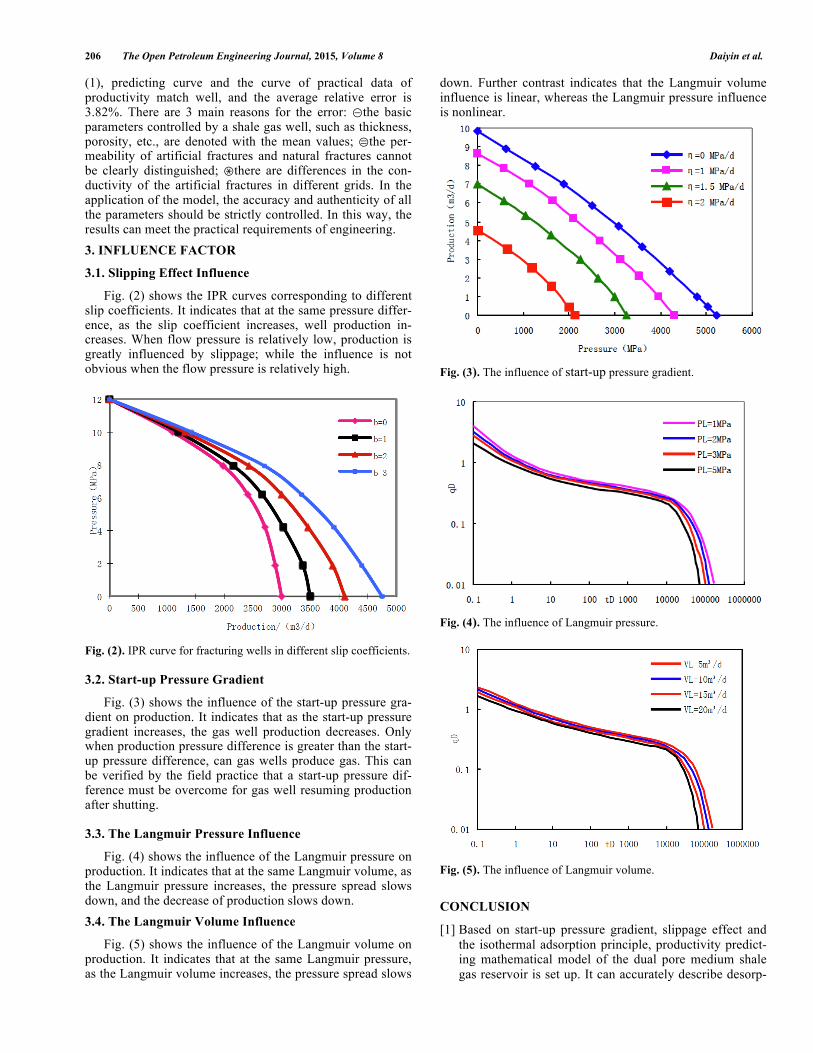
Fig. (3) shows the influence of the start-up pressure gra-dient on production. It indicates that as the start-up pressure gradient increases, the gas well production decreases. Only when production pressure difference is greater than the start-up pressure difference, can gas wells produce gas. This can be verified by the field practice that a start-up pressure dif-ference must be overcome for gas well resuming production after shutting. 3.3. The Langmuir Pressure Influence

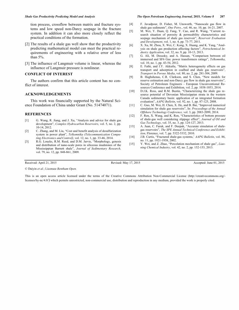
Fig. (4) shows the influence of the Langmuir pressure on production. It indicates that at the same Langmuir volume, as the Langmuir pressure increases, the pressure spread slows down, and the decrease of production slows down. 3.4. The Langmuir Volume Influence

Fig. (5) shows the influence of the Langmuir volume on production. It indicates that at the same Langmuir pressure, as the Langmuir volume increases, the pressure spread slows

down. Further contrast indicates that the Langmuir volume influence is linear, whereas the Langmuir pressure influence is nonlinear.

Fig. (3). The influence of start-up pressure gradient.

Fig. (4). The influence of Langmuir pressure.

Fig. (5). The influence of Langmuir volume.

CONCLUSION

[1] Based on start-up pressure gradient, slippage effect and the isothermal adsorption principle, productivity predict-ing mathematical model of the dual pore medium shale gas reservoir is set up. It can accurately describe desorp-

Shale Gas Productivity Predicting Model and Analysis The Open Petroleum Engineering Journal, 2015, Volume 8 207

tion process, crossflow between matrix and fracture sys-tems and low speed non-Darcy seepage in the fracture system. In addition it can also more closely reflect the practical conditions of the formation.

[2] The results of a shale gas well show that the productivity predicting mathematical model can meet the practical re-quirements of engineering with a relative error of less than 5%.

[3] The influence of Langmuir volume is linear, whereas the influence of Langmuir pressure is nonlinear.

CONFLICT OF INTEREST

The authors confirm that this article content has no con-flict of interest.

ACKNOWLEDGEMENTS

This work was financially supported by the Natural Sci-ence Foundation of China under Grant (No. 51474071).

REFERENCES [1] G. Wang, R. Jiang, and J. Xu, “Analysis and advice for shale gas

development”, Complex Hydrocarbon Reservoirs, vol. 5, no. 2, pp. 10-14, 2012.

[2] C. Zhang, and M. Liu, “Cost and benefit analysis of desulfurization system in power plant”, Telkomnika (Telecommunication Compu-ting Electronics and Control), vol. 12, no. 1, pp. 33-46, 2014.

[3] R.G. Loucks, R.M. Reed, and D.M. Jarvie, “Morphology, genesis and distribution of nano-scale pores in siliceous mudstones of the Mississippian Barnett shale”, Journal of Sedimentary Research, vol. 79, no. 12, pp. 848-861, 2009.

[4] F. Javadpour, D. Fisher, M. Unsworth, “Nanoscale gas flow in shale gas sediments”, One Petro., vol. 46, no. 10, pp. 16-21, 2007.

[5] M. Wei, Y. Duan, Q. Fang, Y. Cao, and R. Wang, “Current re-search situation of porosity & permeability characteristics and seepage mechanism of shale gas reservoir”, Reservoir Evaluation and Development, vol. 1, no. 4, pp. 73-77, 2011.

[6] X. Xu, M. Zhou, X. Wei, C. Kong, X. Huang, and K. Yang, “Anal-ysis on shale gas production affecting factors”, Petrochemical In-dustry Application, vol. 32, no. 9, pp. 10-13, 2013.

[7] G. Ali, M. Dessoky, and A. Hassan, “Comparison between oil immersed and SF6 Gas: power transformers ratings”, Telkomnika, vol. 10, no. 1, pp. 43-54, 2012.

[8] E. Fathi, and I.Y. Akkutlu, “Matrix heterogeneity effects on gas transport and adsorption in coalbed and shale gas reservoirs”, Transport in Porous Media, vol. 80, no. 2, pp. 281-304, 2009.

[9] B. Haghshenas, C.R. Clarkson, and S. Chen, “New models for reserve estimation and non-Darcy gas flow in shale gas reservoirs”, Society of Petroleum Engineers - European Unconventional Re-sources Conference and Exhibition, vol. 2, pp. 1038-1053, 2014.

[10] D.J.K. Ross, and R.M. Bustin, “Characterizing the shale gas re-source potential of Devonian Mississippian strata in the western Canada sedimentary basin: application of an integrated formation evaluation”, AAPG Bulletin, vol. 92, no. 1, pp. 87-125, 2008.

[11] C. Guo, M. Wei, H. Chen, X. He, and B. Bai, “Improved numerical simulation for shale gas reservoirs”, In: Proceedings of the Annual Offshore Technology Conference, vol. 3, pp. 2083-2099, 2014.

[12] F. Ren, X. Wang, and K. Ren, “Characteristics of bottom pressure of shale-gas well considering slippage effect”, Journal of Oil and Gas Technology, vol. 35, no. 3, pp. 124-127, 2013.

[13] A. Juan, C. Faruk, and F. Deepak, “Accurate simulation of shale-gas reservoirs”, The SPE Annual Technical Conference and Exhibi-tion, Florence, vol. 7, pp. 5322-5332, 2010.

[14] J.B. Curtis, “Fractured shale-gas systems,’ AAPG Bulletin, vol. 86, no. 11, pp. 1921-1938, 2002.

[15] Y. Wei, and Z. Zhao, “Percolation mechanism of shale gas”, Liao-ning Chemical Industry, vol. 42, no. 2, pp. 152-153, 2013.

Received: April 21, 2015 Revised: May 17, 2015 Accepted: June 01, 2015

© Daiyin et al.; Licensee Bentham Open.

This is an open access article licensed under the terms of the Creative Commons Attribution Non-Commercial License (http://creativecommons.org/-licenses/by-nc/4.0/) which permits unrestricted, non-commercial use, distribution and reproduction in any medium, provided the work is properly cited.