Embed Size (px)
Citation preview
www.ssoar.info
Production Risk, Pesticide Use and GM CropTechnology in South AfricaShankar, Bhavani; Bennett, Richard; Morse, Steve
Postprint / PostprintZeitschriftenartikel / journal article
Zur Verfügung gestellt in Kooperation mit / provided in cooperation with:www.peerproject.eu
Empfohlene Zitierung / Suggested Citation:Shankar, Bhavani ; Bennett, Richard ; Morse, Steve: Production Risk, Pesticide Use and GM Crop Technology in SouthAfrica. In: Applied Economics 40 (2008), 19, pp. 2489-2500. DOI: http://dx.doi.org/10.1080/00036840600970161
Nutzungsbedingungen:Dieser Text wird unter dem "PEER Licence Agreement zurVerfügung" gestellt. Nähere Auskünfte zum PEER-Projekt findenSie hier: http://www.peerproject.eu Gewährt wird ein nichtexklusives, nicht übertragbares, persönliches und beschränktesRecht auf Nutzung dieses Dokuments. Dieses Dokumentist ausschließlich für den persönlichen, nicht-kommerziellenGebrauch bestimmt. Auf sämtlichen Kopien dieses Dokumentsmüssen alle Urheberrechtshinweise und sonstigen Hinweiseauf gesetzlichen Schutz beibehalten werden. Sie dürfen diesesDokument nicht in irgendeiner Weise abändern, noch dürfenSie dieses Dokument für öffentliche oder kommerzielle Zweckevervielfältigen, öffentlich ausstellen, aufführen, vertreiben oderanderweitig nutzen.Mit der Verwendung dieses Dokuments erkennen Sie dieNutzungsbedingungen an.
Terms of use:This document is made available under the "PEER LicenceAgreement ". For more Information regarding the PEER-projectsee: http://www.peerproject.eu This document is solely intendedfor your personal, non-commercial use.All of the copies ofthis documents must retain all copyright information and otherinformation regarding legal protection. You are not allowed to alterthis document in any way, to copy it for public or commercialpurposes, to exhibit the document in public, to perform, distributeor otherwise use the document in public.By using this particular document, you accept the above-statedconditions of use.
Diese Version ist zitierbar unter / This version is citable under:http://nbn-resolving.de/urn:nbn:de:0168-ssoar-239980

For Peer Review
Production Risk, Pesticide Use and GM Crop Technology in South Africa
Journal: Applied Economics Manuscript ID: APE-05-0480.R1
Journal Selection: Applied Economics
JEL Code:Q12 - Micro Analysis of Farm Firms, Farm Households, and Farm Input Markets < Q1 - Agriculture < Q - Agricultural and Natural Resource Economics
Keywords: Genetically Modified Crops, Production Risk, Biotechnology, South Africa
Editorial Office, Dept of Economics, Warwick University, Coventry CV4 7AL, UK
Submitted Manuscript
For Peer Review
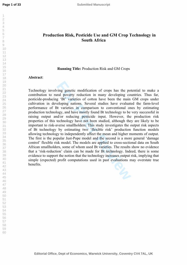
Production Risk, Pesticide Use and GM Crop Technology in South Africa
Running Title: Production Risk and GM Crops
Abstract:
Technology involving genetic modification of crops has the potential to make a contribution to rural poverty reduction in many developing countries. Thus far, pesticide-producing ‘Bt’ varieties of cotton have been the main GM crops under cultivation in developing nations. Several studies have evaluated the farm-level performance of Bt varieties in comparison to conventional ones by estimating production technology, and have mostly found Bt technology to be very successful in raising output and/or reducing pesticide input. However, the production risk properties of this technology have not been studied, although they are likely to be important to risk-averse smallholders. This study investigates the output risk aspects of Bt technology by estimating two ‘flexible risk’ production function models allowing technology to independently affect the mean and higher moments of output. The first is the popular Just-Pope model and the second is a more general ‘damage control’ flexible risk model. The models are applied to cross-sectional data on South African smallholders, some of whom used Bt varieties. The results show no evidence that a ‘risk-reduction’ claim can be made for Bt technology. Indeed, there is some evidence to support the notion that the technology increases output risk, implying that simple (expected) profit computations used in past evaluations may overstate true benefits.
Page 1 of 33
Editorial Office, Dept of Economics, Warwick University, Coventry CV4 7AL, UK
Submitted Manuscript
123456789101112131415161718192021222324252627282930313233343536373839404142434445464748495051525354555657585960

For Peer Review
1
Production Risk, Pesticide Use and GM Crop Technology in
South Africa
I. Introduction
Genetically Modified (GM) crop technology is a potentially powerful addition to the toolkit
for poverty alleviation in rural areas of developing countries. GM technology may provide
answers to agricultural problems that conventional plant breeding methods have not been able
to address adequately in the developing world (Nuffield Council for Bioethics (2003)). The
promise held out is not restricted to larger, richer farmers; Given appropriate institutional
conditions, GM technology is also seen as being capable of benefiting small, resource-poor
farmers (FAO, 2004).
Bacillus Thuringensis (Bt) varieties of cotton and maize, first commercialized by Monsanto,
Inc., are now the most widespread types of GM crops in the developing world. The Bt gene
contained in Bt varieties produces a natural insecticide that acts specifically on a class of
troublesome pests (notably bollworms) that regularly decimate crops in developing countries.
Since its introduction in South Africa in 1998, Bt varieties, particularly of cotton, have been
taken up by farmers in several other developing countries, notably the extremely populous
and largely rural China and India.
Rigorous farm-level performance evaluation of the first generation of Bt varieties has been
conducted in the main adopting countries, and this first generation of results by and large
indicate that Bt technology has been a noteworthy success. Two types of benefits have been
reported, pesticide reduction and yield increase. In China, the extant level of pesticide use in
cotton is very high, and pesticides are generally thought to be overused (applied beyond the
economic optimum). In this case, the contribution of the Bt variety has been to enable a
Page 2 of 33
Editorial Office, Dept of Economics, Warwick University, Coventry CV4 7AL, UK
Submitted Manuscript
123456789101112131415161718192021222324252627282930313233343536373839404142434445464748495051525354555657585960

For Peer Review
2
substantial reduction in pesticide (over)use, with only a marginal effect on yields. These
results have been reported and analyzed in Pray, et. al. (2001) and Huang, et. al. (2003). On
the other hand, in South Africa and India, pesticide inputs are more likely to be underused
(applied below the economic optimum) due to credit and labour availability constraints and
market failure problems associated with the availability of timely supplies. Here, the
contribution of the Bt variety has been to increase yields substantially, with modest changes
in pesticide use. These results are reported and discussed in, among others, Qaim and
Zilberman (2003); Thirtle, et. al. (2002); Shankar and Thirtle (2005); Qaim (2003); Qaim and
de Janvry (2005).
All the studies mentioned above have undertaken their farm-level performance evaluation via
the estimation of production technology, with a dummy variable representation for the use of
Bt technology. Standard production functions have been estimated, in Qaim (2003), Qaim and
Zilberman (2003) and Qaim and de Janvry (2005). ‘Damage Control’ production functions,
which account for the special, damage abating nature of pesticide inputs and Bt technology,
have been used in all the previous studies with the exception of Thirtle et. al. (2002). Thirtle
et. al. instead used a stochastic frontier representation of technology. Almost without
exception, these studies indicate superior performance of Bt varieties relative to local
counterparts.
Valuable as the information contained in these studies is, it is important to note that the
representations of production technology used in the above studies do not consider the
production risk element. Agricultural production is inherently risky, and smallholders in
developing countries are likely very risk-averse. More complete production impact evaluation
of inputs and technologies will therefore need consideration of their interactions with the
riskiness of output. Thus it has been long recognized in the agricultural economics literature
that it is important to allow inputs, particularly pesticides (and therefore technologies that
embody pesticides, such as Bt), to freely affect variance and higher moments of output.
Page 3 of 33
Editorial Office, Dept of Economics, Warwick University, Coventry CV4 7AL, UK
Submitted Manuscript
123456789101112131415161718192021222324252627282930313233343536373839404142434445464748495051525354555657585960

For Peer Review
3
However, typically employed production functions, such as the Quadratic and the Cobb-
Douglas, do not allow production inputs and technologies to flexibly affect variance and
higher moments of output (Just and Pope, 1979). This is also true of the standard damage
control production functions (Saha, et. al., 1997) and stochastic frontier functions (Battese,
Rambaldi and Wan, 1997). Thus these studies only consider the effect of technology on the
expected value of output.
The objective of this paper is to help reduce this gap in knowledge about the production risk
impact of Bt technology1. It accomplishes this by applying two ‘flexible risk’ production
function models to the South African cotton smallholder data previously reported in Thirtle
et. al. (2002) and Shankar and Thirtle (2005). The first model, which applies a Just-Pope
production function (Just and Pope, 1979) to the data, is seen as a preliminary step prior to the
application of a second, more complex model. This second model is an adaptation of Saha et.
al.’s (1997) model which incorporates flexible risk properties while retaining the ‘damage
control’ representation of pesticides and Bt technology. From both models, we simply wish to
test the hypothesis that Bt technology reduces yield (output) risk. To our knowledge, no
previous studies have empirically measured the production risk properties of Bt technology in
a developing country setting.
If the risk-reduction hypothesis is confirmed, GM technology can be said to possess an
additional ‘insurance’ function beyond the pesticide reduction/yield increase attributes
analyzed before. The benefits from the technology would then include a positive risk
premium obtained in addition to benefits (expected value of profits) obtained from mean
output increases. On the other hand, a risk-increasing result would imply that computed
profits overstate the true benefits from the technology. Thus the study of the risk properties is
important for more complete impact evaluation of Bt technology.
Page 4 of 33
Editorial Office, Dept of Economics, Warwick University, Coventry CV4 7AL, UK
Submitted Manuscript
123456789101112131415161718192021222324252627282930313233343536373839404142434445464748495051525354555657585960

For Peer Review
4
Section II proceeds by considering the analytic insights available from previous literature on
how pesticides, and thus Bt technology, may affect risk. Section III sets out the empirical
framework, and section IV presents and discusses the results. Section V concludes and offers
suggestions for future work.
II. Analytical Background
The simple bioeconomics of pesticides and risk
Bt technology embodies a pesticide, and hence notions relating to the risk effects of Bt
technology are parallel to those concerning conventional pesticides. While there is intuitive
appeal on the surface to suggest that pesticides should decrease risk, Pannell (1991) suggests
that this is misleading, and several empirical studies instead find a risk-increasing effect (eg.
Antle (1988); Horowitz and Lichtenberg (1993)). Horowitz and Lichtenberg (1994) provide
an elegant exposition explaining why a risk-increasing effect is at least as plausible as a risk-
decreasing effect. We lean heavily on their exposition in heuristically outlining the arguments
below.
Consider a production function, f(z, x, e), where z is pesticide input, x is a vector of all other
inputs, and e is random production error. Without loss of generality, suppose e is ordered
from bad states of nature to good states of nature, implying fe(z, x, e) > 0 where the subscript
denotes the partial derivative. We would expect pesticide to not decrease output in any state
of nature, i.e., fz(z, x, e) > 0. Risk averse producers may be characterized as choosing (z, x) to
solve Max ∫U(pf(z, x, e) - wzz – wxx)de , where U(.) is the utility function, p is output price,
wz is pesticide price and wx is the vector of other input prices. Then input z can be said to be
risk-decreasing (increasing) if fze(z, x, e) < 0, i.e., z increases output more in bad (good) states
of nature than in good (bad). Quiggin (1991) demonstrates that this definition is equivalent to
alternative definitions of risk-decreasing (increasing) inputs used in the literature, such as that
Page 5 of 33
Editorial Office, Dept of Economics, Warwick University, Coventry CV4 7AL, UK
Submitted Manuscript
123456789101112131415161718192021222324252627282930313233343536373839404142434445464748495051525354555657585960

For Peer Review
5
more risk-averse producers use more (less) of risk-decreasing (increasing) inputs than less
risk averse producers, all else equal. If e mainly represented randomness of pest density, then
we have the conventional wisdom that pesticide and Bt technology should be risk-decreasing,
since they raise output more in bad states of nature, i.e., when pest density is high.
Intuitive as this logic seems, Horowitz and Lichtenberg (1994) show that it is untenable when
alternative or multiple sources of uncertainty are considered. In developing country
agricultural situations such as the rainfed cotton cultivation case we consider, rainfall, or crop
growth conditions more generally, are at least as important as sources of randomness as pest
density. In a situation where pest density is relatively stable, but there is considerable
uncertainty over rainfall, rainfall becomes the main source of randomness in e. In such a case,
during the good states of nature (high rainfall) there is more crop to save given the pest
density, and pesticides raise output more in this good state of nature, making pesticide a risk-
increasing input. In many agricultural situations, both sources of randomness, pest density and
rainfall, are important. More so, they are likely to be negatively correlated, i.e. pest density is
high (bad state of nature with regard to pest density) when rainfall is high (good state of
nature with regard to rainfall). In cases of strong negative correlation between these two,
Horowitz and Lichtenberg’s analysis suggests again that pesticides are likely to be risk-
increasing.
Thus, we are able to take away two major lessons from this previous literature:
(i) The risk effect of pesticides and Bt-technology can differ from situation to situation, and is
a matter for empirical determination in any given situation, and
(ii) It may be important to explicitly account for multiple sources of randomness in empirical
analysis.
Note, however, that even though the above bioeconomic framework goes significantly beyond
the standard production framework in its consideration of risk, ground realities can be more
Page 6 of 33
Editorial Office, Dept of Economics, Warwick University, Coventry CV4 7AL, UK
Submitted Manuscript
123456789101112131415161718192021222324252627282930313233343536373839404142434445464748495051525354555657585960

For Peer Review
6
complex still. High rainfall may not always represent a good state of nature even in the
absence of pest considerations. The effect would depend on the amount of rainfall at various
stages of plant growth. Rainfall and pest control interactions may also be affected by
considerations such as pesticide wash-off caused by high rainfall. In Makhathini, there is
anecdotal evidence that the latter effect might have occurred in the season for which our
analysis has been conducted. However, consideration of such effects requires much more
detailed data than are available to us, and is thus beyond the scope of this paper. Work by
Antle (1983; 1988) provides an example of how pest control input determination can
be viewed as a sequential problem, and how data from multiple stages during the
season can be used to enhance empirical production models.
Risk and damage abatement properties of production functions
Conventional production functions are incapable of displaying flexible risk properties.
Production functions additive in the error term, such as the Quadratic, do not allow inputs to
either decrease or increase risk. In other words, where f(z, x, e) = g(z, x) + e, fze = 0. Those
with mutiplicative exponential error terms, such as the Cobb-Douglas and the Translog only
allow risk-increasing effects, i.e., where f(z, x, e) = g(z, x)expe, fze > 0. Apart from their
inflexibility in allowing the data to determine risk properties, these production functions also
lump all sources of randomness into a single error term. Another critical shortcoming for
agricultural applications is that they treat all inputs symmetrically, not accounting for the
special nature of inputs like pesticides. The last point is also true of ‘stochastic production
functions’ such as the Just-Pope production functions, y = q(z, x) + h(z, x)e, which are able to
allow flexible risk properties, but do not account for the special, damage abating nature of
pesticide inputs.
Page 7 of 33
Editorial Office, Dept of Economics, Warwick University, Coventry CV4 7AL, UK
Submitted Manuscript
123456789101112131415161718192021222324252627282930313233343536373839404142434445464748495051525354555657585960

For Peer Review
7
Lichtenberg and Zilberman (1986) presented a critique of traditional production functions,
and offered an alternative, more intuitive way to model the role of pesticide in the agricultural
production process. Drawing inspiration from the bioeconomic literature, they posited that
pesticides belong to a class of ‘damage control’ inputs. Damage control inputs are different
from conventional inputs in that they affect output only indirectly, by reducing the extent of
damage in the event that damage occurs. In contrast, conventional inputs such as fertilizer and
labour increase output directly.
If y denotes output, x is a vector of ‘conventional’ inputs, and z is the damage control
(pesticide), then y = f( x, g(z) ), with f(.) concave in x and g(z). g(z), the ‘abatement function’,
is defined on the [0, 1] interval and is increasing in z. as z increases, 1)z(g and
)x(fy , i.e., a greater part of maximum potential output is realized. As z decreases,
0)z(g , and )0,x(fy , i.e., output falls towards the level consistent with maximum
destructive capacity. For reasons of econometric identification, the practice in empirical work
is to simplify the damage control function to a proportional one, i.e., y = f(x)g(z).
In the context of pest management, the above specification implies that as pesticide input z
increases, abatement 1)z(g , and at the limit y = f(x), i.e., there is no destruction due to
pest damage and maximum potential output is realized. As pesticide application declines
towards 0, 0)z(g , and 0y . Since y is now proportional to g(z) and g(z) is between 0
and 1, g(z) represents the percentage of maximum potential output realized for a given level
of pesticide use, z. Since g(z) lies in the [0,1] interval, a choice of several cumulative
distribution functions is available to model g(z), with the Weibull, Exponential and Logistic
widely used in applications. Where the damage control representation is appropriate,
Lichtenberg & Zilberman demonstrate that using conventional specifications can lead to
serious bias and erroneous conclusions about the productivity and use efficiencies of
pesticides as well as the other conventional inputs included in the analysis.
Page 8 of 33
Editorial Office, Dept of Economics, Warwick University, Coventry CV4 7AL, UK
Submitted Manuscript
123456789101112131415161718192021222324252627282930313233343536373839404142434445464748495051525354555657585960

For Peer Review
8
As discussed before, most of the Bt cotton evaluation papers have accordingly used damage
control specifications in their analysis. However, even though this corrects the potential bias
caused by the special nature of pesticide inputs, it does not provide flexibility with regard to
risk effects. It is easy to show that the usual damage control functions cannot allow mean and
variance effects of inputs (or technologies) to be qualitatively independent of each other.
Damage control specification with flexible risk properties
The above discussion points to the need for a specification that allows a damage control
characterization for pesticide and Bt technology, flexible risk properties for the input and the
technology, and explicit accounting for multiple sources of uncertainty. Saha, Shumway and
Havenner (1997) present such a model (henceforth referred to as the SSH model), which we
use as the main basis for our empirical work. Their model is described briefly below.
The SSH production function is described by:
y = f(x, β) g(z, α, e) exp(ε) (1)
Here, β is a vector of parameters attached to the ‘conventional’ inputs in x, while α is the
parameter vector attached to the ‘damage control’ inputs in z. A key difference relative to the
ordinary damage control function specification is that (1) contains two error terms: e, attached
to the damage control function g(.), that represents pest and pesticide application related
randomness, and ε, related to randomness in crop growth conditions such as rainfall
variability. e and ε are allowed to be correlated. The SSH model makes two key assumptions
that facilitates the identification and estimation of the model: (i) The damage control function
is specified as g(z, α, e) = exp[-A(z, α)e], where A(.) is a continuous and differentiable
function, and (ii) ε ~ N(0, 1), e ~ N(μ, 1) and cov(ε, e) = ρ. This specification gives:
Page 9 of 33
Editorial Office, Dept of Economics, Warwick University, Coventry CV4 7AL, UK
Submitted Manuscript
123456789101112131415161718192021222324252627282930313233343536373839404142434445464748495051525354555657585960

For Peer Review
9
In(y) ~ N[ ln f(.) – μA(.), B(.)] (2)
where B(.) ≡ [1 + A(.)2 – 2A(.)ρ]. A log-likelihood function can be easily derived under this
specification, and estimation can use standard nonlinear optimization methods. One
implication of the SSH model is that output is distributed lognormally. Although there may be
other parametric distributions that describe farm output better, the lognormal does have a
history of farm output applications (e.g. Sherrick, et. al, (2004); Saha et. al., (1997);
Tirupattur, et. al. (1996)). Most importantly, Saha, et. al. demonstrate that marginal effects of
inputs and technologies contained in g(.) on the variance of output can be either positive or
negative, and independent of the marginal effects on the expected value of output. In other
words, flexibility with respect to risk is achieved while retaining the damage control
specification.
Two comments are worth making at this stage:
(i) With the two error terms as specified in (1), the SSH model has a resemblance to
stochastic frontier models. Indeed, all damage control production functions are similar in
spirit to stochastic frontier models, since both types of models posit a maximum possible
output f(x), with firms achieving some proportion of that output. The SSH model is closer to
stochastic frontier specifications, given that it incorporates two, instead of one, error terms.
However, standard stochastic control specifications do not allow correlation between the two
error terms.
(ii) We have started referring to marginal effects of inputs and technologies on variance,
rather than on risk. As is well known, these are not generally equivalent. It is fully
acknowledged here that theoretical assumptions are necessary to obtain equivalence. The first
model we use, the Just-Pope production function, assumes normality of output. With this
model, variance and risk effects are equivalent since the normal follows the location-scale
condition of Meyer (Meyer (1989); Leathers and Quiggin (1991)). In the SSH model, output
Page 10 of 33
Editorial Office, Dept of Economics, Warwick University, Coventry CV4 7AL, UK
Submitted Manuscript
123456789101112131415161718192021222324252627282930313233343536373839404142434445464748495051525354555657585960

For Peer Review
10
is lognormally distributed. The lognormal does not follow the location-scale condition in spite
of its two-parameter nature. However, if the utility function is characterized by constant
relative risk aversion (CRRA) and the random variable is lognormally distributed, Newberry
and Stiglitz (1981) show that the necessary equivalence is obtained. Thus we invoke the
CRRA assumption. While the assumption is open to debate (see Wik, et. al. (2004) and
Miyata (2003) for a discussion of and evidence against this assumption in agricultural
settings) we note that CRRA is often employed in analysis in agricultural economics (e.g.
Myers (1989); Pope and Just (1991)).
III. Empirical Matters
Empirical setting
The empirical focus is on cotton growing smallholders in Makhathini flats, Kwa-Zulu Natal,
South Africa (described extensively in Ismael et. al. (2002); Gouse, et. al. (2002)). About
3,000 Zulu smallholders growing rainfed cotton in Makhathini Flats, and another 500 in
Tonga, in Mpumalanga together account for about 98% of smallholder cotton grown in South
Africa (Hofs and Kirsten, 2002). In 1998/99, with strong support provided by a private input
supply company called VUNISA, a few smallholders in Makhathini Flats started planting a Bt
cottonseed variety, NuCOTN 37-B. This insecticide produced by this variety provides
resistance to bollworm, which is the most troublesome class of pests in the area, followed by
cotton aphids and jassids. The Bt gene, used by Delta Pineland in developing NuCOTN 37-B,
belongs to Monsanto. In addition to a premium payable per bag of Bt seed over conventional
seed, Bt users also pay a technology fee. At the time of the data collection for this research,
VUNISA Cotton was the sole supplier of seed, chemicals and support services for the farmers
through their extension officers, including credit for land preparation, chemicals and seed,
based on their credit history. VUNISA bought cotton from the farmers at prices fixed by
Cotton South Africa, but has faced competition from a new gin since 2002. Diffusion of the
technology was very rapid in the initial years, with some estimates putting the adoption rate at
Page 11 of 33
Editorial Office, Dept of Economics, Warwick University, Coventry CV4 7AL, UK
Submitted Manuscript
123456789101112131415161718192021222324252627282930313233343536373839404142434445464748495051525354555657585960

For Peer Review
11
90% by 2002/03. Reports suggest that significant disadoption has occurred since then due to
the removal of institutional support (credit and buy-back guarantees initially offered by
VUNISA).
Agriculture is the main livelihood source in Makhathini. Smallholder farms grow between 1
and 3 hectares of rainfed cotton. Some maize and beans are grown, predominantly for
subsistence, but cotton occupies the most acreage and is the main source of cash income.
Smallholder cotton cultivation in the area is marked by relatively low yields. Irrigated cotton
yields in China, for example, are on average in excess of 3000 kg/ha, while smallholder dry
land cotton yields in Makhathini seldom exceeded 600 kg/ha prior to the introduction of Bt
technology. Lack of irrigation is a major constraining factor.
Data
The dataset for the 1999-00 cotton season that we use has been discussed in detail by Thirtle
et. al. (2003) and Shankar and Thirtle (2005), and so we restrict ourselves to a brief sketch.
Survey data were originally obtained on 100 Makhatini cotton smallholders. After deletion of
observations with missing values, and removal of outliers, 86 observations were used in
analysis here, with 58 Bt adopters and 33 non-Bt farmers. The data included quantities of
inputs and outputs, cost and revenue information for the cotton crop, as well as information
on a set of socio-economic variables. Sample means for the key variables are presented in
Table 1.
Table 1 about here.
Information in Table 1 reveals that Bt provided a substantial yield advantage in the year 1999-
2000. It also enabled pesticide application to be lowered considerably. Note that adoption in
Makhathini flats was characterized by complete adoption or non-adoption (Thirtle, et. al.,
2003), i.e. the data do not contain partial adopters. One additional aspect of interest is that the
Page 12 of 33
Editorial Office, Dept of Economics, Warwick University, Coventry CV4 7AL, UK
Submitted Manuscript
123456789101112131415161718192021222324252627282930313233343536373839404142434445464748495051525354555657585960

For Peer Review
12
adopters on average had a significantly larger farm size. This reflects a policy adopted by
VUNISA of targeting larger farmers in the early years (Shankar and Thirtle, 2005) and is
further discussed below in the context of selectivity issues in estimation.
Estimation details:
All the production functions estimated in this article assume constant returns to scale and use
a per-hectare specification for output and variable inputs. This is in line with most of the
previous literature on Bt cotton impact assessment cited before, and also helps attenuate
multicollinearity problems resulting from strong correlation between land and variable inputs
such as pesticide and seed. Also, logic dictates that farm level applications of damage control
models should specify at least pesticide input on a standardized (per-hectare), rather than on a
whole farm basis. Since the abatement function g(z) is a proportion, expressing z on a whole
farm basis would give misleading results. Henceforth, when we refer to the output y or the
input sets (x, z), the implication is that all of these are expressed on a per-hectare basis.
The first model applied to the data is the Just-Pope production function, given by
y = q(z, Bt, x, α) + h(z, Bt, x, β)e, e ~ N(0, 1) (3)
Here, Bt represents a dummy variable, 1=Bt adopter, 0=non-adopter, and the rest of the
notation is as before. Under this Just-Pope setup, expected value of output, E(y) = q(z, Bt, x),
while variance of output V(y) = h2(z, Bt, x), allowing all inputs as well as Bt technology to
affect output variance independently of effects on the mean of output.
Cobb-Douglas forms are used in q(.) and h(.), i.e.
(4)
Btpestlabfertseed
Btpestlabfertseed exp)z()x()x()x(A(.)q
Btpestlabfertseed
Btpestlabfertseed zxxxBh exp)()()()((.)
Page 13 of 33
Editorial Office, Dept of Economics, Warwick University, Coventry CV4 7AL, UK
Submitted Manuscript
123456789101112131415161718192021222324252627282930313233343536373839404142434445464748495051525354555657585960
For Peer Review
13
In (4), xseed, xfert, xlab and zpest represent seed, fertilizer, labour and pesticide inputs,
respectively, Bt is the Bt dummy variable, and (A, B, α, β) is the parameter set to be
estimated. Although the Cobb-Douglas form is restrictive, it proved to be the most practical
choice for estimation here due to the relatively small sample size. Besides the problem with
conserving degrees of freedom, alternative forms such as the quadratic and the translog were
found to worsen extant collinearity problems.
The estimation of (3) was accomplished using the three-step process originally described by
Just and Pope (1979). Suppose i indexes the farmers. First, a nonlinear least squares (NLS)
regression yi = q(zi, Bti, xi, α) + ei* was estimated, resulting in first round estimates of α.
Given (3), this is a heteroskedastic regression. The second step involved an OLS regression
of ln|ei*| (using ei* estimated from the first step) on ln [h(zi, Bti, xi, β)], to provide estimates of
β. Finally, a NLS regression of
produced revised estimates of α . Just and Pope (1978) show that the resultant estimates are
consistent and asymptotically efficient.
The SSH model features have already been described in section II. To recap, we estimated
yi = f(xi, β) exp[-A(zi, Bti, α)ei]exp(εi), εi ~ N(0, 1), ei ~ N(μ, 1), cov(εi, ei) = ρ (5)
Saha, et. al. (1997) derive the loglikelihood function (LLF) for this model, given by:
LLF(α, β, μ, ρ) =
i i
2iii
i (.)B
](.)A(.)flny[ln(.)Bln
2
12ln
2
n(6)
where Bi(.) ≡ [1 + Ai(.)2 – 2Ai(.)ρ]. We estimated the parameter vector (α, β, μ, ρ) by
maximizing (6) directly.
)ˆ,Bt,z(h),Bt,z(qon)ˆ,Bt,z(hy ii1
iiii1
i β,xα,xβ,x iii
Page 14 of 33
Editorial Office, Dept of Economics, Warwick University, Coventry CV4 7AL, UK
Submitted Manuscript
123456789101112131415161718192021222324252627282930313233343536373839404142434445464748495051525354555657585960

For Peer Review
14
Alternative functional forms were experimented with for f(.) and A(.) 2, and a decision was
made to use Cobb-Douglas forms for both functions. Ease of convergence in nonlinear
estimation was a key factor in making this decision. Saha et. al. in their original application
used a Cobb-Douglas form for f(.) and a linear form for A(.). Note, however, that a linear
form sits uneasily with the abatement function interpretation of exp[-A(.)]. To take a simple
example, if A(z, α) = α0 + α1z, to keep abatement within the [0,1] interval and to have a
positive marginal product for z, it would be necessary to have α0 > 0 and α1 < 0. However, the
implication then is that beyond a certain value for z, A(.) would become negative, and
abatement exp[-A(.)] > 1. The Cobb-Douglas form improves on the linear specification in this
regard3, and also has the virtue of parsimony.
Selectivity
Selectivity can be a serious issue in production function estimation of farm-level impacts of a
technology using cross-sectional data. While survey datasets such as the one used in this
research may contain information on both adopter and non-adopters, there is usually no
random assignation of individuals into such groups. There is then the very real possibility
that adoption patterns of individuals are related to their productivity patterns. Often, ‘better’
or more efficient farmers, who are able to get more output out of a given technology and a
given set of inputs, are also the ones to adopt technologies that improve productivity. Thus
production function estimation using cross-sectional data is likely to exaggerate the impacts
of technology adoption, confounding the inherent efficiency of adopting farmers with the
actual performance of the technology itself.
Selectivity is an issue to be considered seriously in farm-level GM crop impact estimation as
well. However, there has been surprisingly little explicit attention devoted to this issue in the
literature. Where panel data are available, it is possible to control for farmer-specific effects,
thereby isolating the technology effects accurately. In a cross-sectional context, one solution
is to use Heckman’s correction, where inverse Mills ratios derived from first step adoption
Page 15 of 33
Editorial Office, Dept of Economics, Warwick University, Coventry CV4 7AL, UK
Submitted Manuscript
123456789101112131415161718192021222324252627282930313233343536373839404142434445464748495051525354555657585960

For Peer Review
15
probit models can be used to correct selectivity bias in second step production function
estimation. A common problem with this strategy, however, is that instruments derived from
adoption probits are often poor.
However, as Barnow, Cain and Goldberger (1980) point out, assuming the effects that cause
the sample selection problem are observable, including those variables in the outcome
regression would correct for the sample selection problem. This standard regression based
method has been called ‘ignorability of treatment’ (Rosenbaum and Rubin, 1983), and
‘selection on observables’ (Heckman and Robb, 1985) in the literature. Loosely, treatment is
random/ignorable conditional on those variables that affect both selection and outcomes. In
Makhathini, Shankar and Thirtle (2005) have argued that farm size was the main variable
determining adoption. VUNISA launched the technology by promoting it to larger farmers in
the initial years, with the expectation that smaller farmers would be picked up via copy
adoption in later years. Indeed, farm size was the only strongly significant variable in
adoption models reported by Thirtle et. al. (2003) and Shankar and Thirtle (2005). Thus,
inclusion of a farm size variable in our production function regressions may be an effective
control for any existing selectivity. Other socio-economic variables such as farmer education
and age have also been used in production functions estimated in the Bt cotton literature (eg.
Qaim 2003; Qaim and de Janvry, 2005). A similar set was used in initial runs in this research.
However, these other variables were largely insignificant in all regressions. The farm size
variable alone was retained in the final set of estimates, because of farm size being a potential
determinant of yields and also because of its role in selectivity control.
IV. Results
Just-Pope production function results
Page 16 of 33
Editorial Office, Dept of Economics, Warwick University, Coventry CV4 7AL, UK
Submitted Manuscript
123456789101112131415161718192021222324252627282930313233343536373839404142434445464748495051525354555657585960

For Peer Review
16
As noted before, the first step (mean) regression in the three-step procedure is implicitly a
heteroskedastic regression. We therefore tested for heteroskedasticity in the first step. Two
tests were carried out, White’s (1980) test and Breusch & Pagan’s (1979) test. In both tests,
the test statistic is distributed as chi-squared under the null hypothesis of no
heteroskedasticity. The White test makes no assumptions about the form of the
heteroskedasticity and simply tests H0: σ2i = σ2 for all i against H1: Not H0. The Breusch-
Pagan test on the other hand is a Lagrange multiplier test that assumes that if any
heteroskedasticity exists, the error variance varies with a set of regressors. In our case, the
natural set of regressors to use is the set of regressors used in the variance regression step of
the Just-Pope function, i.e., a constant, the three variable inputs, farm size, and the Bt
adoption dummy. The White test value was 56.82, which is considerably in excess of the 95%
level chi-square critical value of 38.80. Thus the White test strongly rejects the null
hypothesis of homoskedasticity. The Breusch-Pagan test value was 25.83, which is also
substantially higher than the 95% level chi-square critical value of 11.07 with 5 degrees of
freedom. The Breusch-Pagan test thus bolsters the evidence provided by the White test that
the null hypothesis of homoskedasticity can be rejected, and provides further rationale for the
investigation of how output variance or risk is affected by inputs and technology.
Table 2 presents the estimates of the mean and variance portions of the Just-Pope production
function, following implementation of the three-step procedure outlined earlier. Even though
the mean portion is estimated as a Cobb-Douglas function with an additive, instead of the
usual exponential error term, it retains an elasticity interpretation. Thus the elasticities of
expected value of yield with respect to the variable inputs are all positive and have plausible
values, although the seed elasticity is insignificant. Increasing farm size is seen to have a
depressing effect on the expected value of yields, although the parameter is significant only at
the 10% level. The Bt dummy variable parameter is the most strongly significant of all, and
the positive value confirms previous findings that Bt varieties provide a strong boost to
(expected value of) yields.
Page 17 of 33
Editorial Office, Dept of Economics, Warwick University, Coventry CV4 7AL, UK
Submitted Manuscript
123456789101112131415161718192021222324252627282930313233343536373839404142434445464748495051525354555657585960
For Peer Review
17
Table 2 about here.
The variance effects of the inputs, seen in the bottom half of the table, are however far weaker
as estimated by the Just-Pope model. A positive (negative) coefficient sign indicates a risk
increasing (decreasing) effect for the input it is attached to. Seed is seen to be the only
variable input with a statistically significant effect on output variance, and that only at the
10% level. The positive sign of the pesticide coefficient indicates a risk increasing effect for
the input. However, it is insignificantly different from zero. The Bt dummy on the other hand,
bears a negative sign indicating a risk-decreasing effect, but is even more strongly
insignificant. Opposing signs for the pesticide and Bt dummy are not in line with
expectations4, and along with the very low t-ratios suggest that the Just-Pope model cannot
confirm any strong evidence for the hypothesis that Bt technology reduces risk.
However, noting again that the Just-Pope function is estimated only as a preliminary step in
the investigation of risk properties, and that it does not have a damage control specification
appropriate for the pesticide and Bt variables, we now turn to results obtained from the SSH
model.
SSH model results
Table 3 presents results from the SSH model. For comparison, we also present results from a
damage control model obtained by imposing restrictions on the SSH model in (5), i.e.,
yi = f(xi, β) exp[-A(zi, Bti, α)]exp(εi), εi ~ N(0, σ2) (7)
Page 18 of 33
Editorial Office, Dept of Economics, Warwick University, Coventry CV4 7AL, UK
Submitted Manuscript
123456789101112131415161718192021222324252627282930313233343536373839404142434445464748495051525354555657585960

For Peer Review
18
With its single error term specification, potential output function f(.) and abatement function
exp[-A(.)], (7) is a traditional damage control function. It can allow only risk-increasing
inputs and technologies, in contrast to the SSH model, (5), which allows the data to determine
the risk effects of inputs and technologies. This damage control model was estimated using
nonlinear least squares.
Table 3 about here
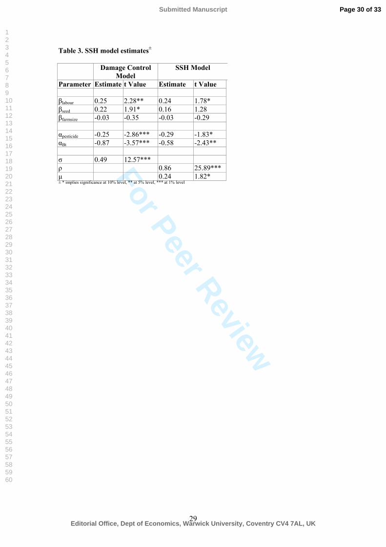
The labour and seed production elasticities from the two models, seen in the top half of Table
3, are not substantially dissimilar to the mean function estimates produced previously by the
Just-Pope model. However, the SSH model produces a somewhat lower and statistically
insignificant estimate for the seed coefficient, 0.16, compared to the significant 0.22 under the
damage control model. The farm size effect is seen to be indistinguishable from zero under
both models. An obvious a-priori expectation is that pesticide input and Bt technology should
not reduce abatement. Equivalently, ∂y/∂zpesticide ≥ 0 and (y|Bt – y|NonBt) ≥ 0, all else held equal.
For these to hold, it can be verified that the coefficients attached to pesticide input and the Bt
technology dummy in the two models need to be non-positive. As can be seen from the table,
this is indeed so. In both models, the negative valued coefficients αpesticide and αBt are also
significant at conventional significance levels, although these coefficients seem more
precisely measured with the damage control model.
As Saha, et. al. note, a necessary condition for rejecting the SSH model in favour of the
damage control one is the restriction ρ=0 where ρ is the covariance between the two random
variables e and ε, since one of the random variables is missing in the damage control model.
Table 3 shows that the estimated value of ρ is highly significant, with a t value of 25.89. Thus
we cannot find evidence to support discarding the SSH model in favor of the simpler damage
control model. ρ has a positive value of 0.86. This positive correlation between pest density
Page 19 of 33
Editorial Office, Dept of Economics, Warwick University, Coventry CV4 7AL, UK
Submitted Manuscript
123456789101112131415161718192021222324252627282930313233343536373839404142434445464748495051525354555657585960

For Peer Review
19
random variable e and rainfall random variable ε would appear to contradict the earlier notion
that e and ε should be negatively correlated. However, this is misleading. It can be calculated
from (5) that ∂y/∂ε >0, i.e., the rainfall random variable is ordered from bad states of nature
(poor rainfall) to good states (good rainfall). However, ∂y/∂e<0, i.e., the pest density random
variable is ordered from good states of natures (low pest density) to bad (high pest density) in
the SSH model (5). Therefore, ρ should indeed be positive. Our finding of a positive, strongly
significant value for ρ is thus consistent with the earlier interpretation of the two random
variables in the model, and lends support for the SSH model in comparison to a simpler
damage control alternative.
The mean and variance effects of pesticide input and Bt technology were calculated at the
sample mean values of the variables. At the baseline, it was assumed that non-Bt technology
was being used, and all other independent variables were being held fixed at overall sample
mean values. Given this baseline, the pesticide effects were calculated as ∂E(y)/∂zpesticide and
∂V(y)/∂zpesticide, i.e., the marginal effects on expected yields and yield variance5 of a one unit
increase in pesticide. The Bt technology effect is a discrete one, where the technology
provides the equivalent of an unknown number of units of pesticide upon adoption. Thus the
Bt effects were calculated as E(y)|Bt – E(y)|Non-Bt and V(y)|Bt – V(y)|Non-Bt, with all other
variables held fixed. These effects were calculated for both the damage control model and the
SSH model. Approximate standard errors were also calculated using the Delta method. The
results are reported in Tables 4 and 5.
Table 4 about here.
Table 5 about here.
Both models in Table 4 are seen to predict a positive and statistically significant effect of
pesticide on expected yields. Indeed, these effects are almost identical across the models.
Turning to the variance effects of a marginal increase in pesticide use, the damage control
Page 20 of 33
Editorial Office, Dept of Economics, Warwick University, Coventry CV4 7AL, UK
Submitted Manuscript
123456789101112131415161718192021222324252627282930313233343536373839404142434445464748495051525354555657585960

For Peer Review
20
model predicts an increase in the variance (risk). As discussed earlier, this is as expected,
since the damage control model forces the variance effect to be in the same direction as the
marginal product. However, the SSH model, which provides flexible risk effects, predicts the
same qualitative risk effect, i.e. that pesticide increases risk. In fact, the increase in yield
variance is significantly higher in the SSH model than in the damage control model, in
response to the same marginal unit increase in pesticide.
Since Bt technology embodies a certain type of pesticide, the expectation is that the mean and
variance effects of Bt technology adoption would be along the same lines as those for
pesticide. This is verified in Table 5. Once again, the mean effects of Bt technology adoption
are positive, strongly significant, and almost identical across the two models. Since Bt
technology is likely to provide the equivalent of several litres of bollworm pesticide during
the season, the technology effect is much stronger than that of a marginal unit of pesticide
seen in Table 4. Under the damage control model, the variance effect of Bt technology is
positive, i.e. risk-increasing, as expected. However, again the SSH model reaffirms this
qualitative finding in a flexible risk setting. Under the SSH model, Bt technology adoption is
found to increase risk. What is more, the increase predicted by this flexible risk model is more
than ten times the quantitative increase found under the damage control model. Although
there is some imprecision in the estimation of this effect under the SSH model, the effect is
nevertheless significant at the 10% level.
Thus neither the Just-Pope model nor the SSH model is able to confirm a strong and
statistically significant risk-decreasing effect for Bt technology. Therefore, the available
evidence does not allow claim of this potentially valuable additional benefit for the
technology in Makhathini. On the contrary, the SSH model predicts a strong risk-increasing
effect. This is intuitively plausible given the bioeconomic theory of pesticide and risk
discussed previously. We have noted before that cotton cultivation in Makhathini is rainfed,
and that lack of irrigation is a major constraining factor. Under these circumstances, rainfall is
Page 21 of 33
Editorial Office, Dept of Economics, Warwick University, Coventry CV4 7AL, UK
Submitted Manuscript
123456789101112131415161718192021222324252627282930313233343536373839404142434445464748495051525354555657585960

For Peer Review
21
likely at least as important a source of randomness as pest density. Where rainfall is relatively
low, there is less crop to protect, and Bt technology is relatively less effective. Where rainfall
is relatively high, there is more crop to protect, and the technology is more effective in raising
marginal cotton product. In other words, the technology in these circumstances is a ‘fair
weather friend’. Even where the rainfall and pest density random variables are strongly
negatively correlated in the Horowitz and Lichtenberg sense (strongly positively correlated
from the SSH model perspective), Horowitz and Lichtenberg have shown that a risk
increasing effect is likely. This strong correlation has been confirmed for our case, and is
consistent with the risk increasing effect we find.
V. Conclusion
This research has investigated an important, but previously unexplored, aspect of GM
technology – it’s production risk aspects. Specifically, we have been interested in testing the
hypothesis that Bt cotton technology reduces risk in South Africa, in addition to the
(expected) yield-boosting effect measured and analyzed by previous studies. The risk notion
is of importance in a developing country smallholder setting since small farmers have
relatively few avenues available to shift risk. The risk aspect is also intimately tied up with
notions of vulnerability that are given much prominence in the poverty literature.
Our review of the bioeconomics of pesticide and risk revealed that the risk effects of this
technology can be hard to predict and are probably situation-dependent. Where multiple
sources of uncertainty abound, such as rainfall and pest-density, depending on the relative
importance of each random variable and the correlation between them, either risk-increasing
or risk-decreasing effects can plausibly be found. The first model applied was a Just-Pope
model that is the workhorse of production risk investigation. In accordance with the notion of
multiple sources of randomness, we also chose to apply the SSH production function model
that can display flexible risk effects in addition to accommodating two distinct sources of
randomness and a damage control representation.
Page 22 of 33
Editorial Office, Dept of Economics, Warwick University, Coventry CV4 7AL, UK
Submitted Manuscript
123456789101112131415161718192021222324252627282930313233343536373839404142434445464748495051525354555657585960

For Peer Review
22
Our results showed that neither model can provide any support for the risk-reduction
hypothesis. The Just-Pope model shows the risk effect of Bt technology to be insignificant,
while the SSH model shows a strong, statistically significant risk-increasing effect. This is
consistent with the notion of rainfall being a key source of randomness in irrigated
smallholder cotton production. Thus a plausible interpretation of the results is that Bt
technology best produces its effects in Makhathini when the going is good, i.e., when the
crop-growth conditions (rainfall) are good.
It must be emphasized that this research is just one preliminary piece in a potentially larger
puzzle concerning GM technology and production risk. There are a number of limitations to
this study, and there is much scope for future investigation. Firstly, risk effects are almost
certainly situation dependent, and so similar applications to other parts of the world are
warranted. Secondly, we have only used cross-sectional data6, and further analysis with panel
data models can provide richer specifications controlling for heterogeneity and selectivity, if
present. To provide an example of how panel specifications might be important, note that one
potential cause of correlation between the random variables e and ε is individual
heterogeneity. Lacking panel data, we have been unable to control for such heterogeneity and
have simply interpreted the correlation in terms of natural production randomness. The Bt
cotton evaluation literature has thus far avoided proper panel-data analysis, even where such
data were available, possibly because of the difficulty of including heterogeneity effects
within nonlinear models such as the damage control ones commonly applied. However,
multiplicative panel data models (Wooldridge, 1997) have potential in this regard, and
Carpentier and Weaver (1999) have shown how these can be adapted to damage control
models. Thirdly, we have only calculated the risk effects of the technology, but have not been
able to further explore implications for the smallholders. This is due to a lack of data for this
study, but where household wealth data are available, it is possible to compute welfare
equivalents of the increased risk for individuals in the data set or for representative agents.
Page 23 of 33
Editorial Office, Dept of Economics, Warwick University, Coventry CV4 7AL, UK
Submitted Manuscript
123456789101112131415161718192021222324252627282930313233343536373839404142434445464748495051525354555657585960

For Peer Review
23
References
Antle, J.M. (1983). Sequential Decision Making in Production Models, American
Journal of Agricultural Economics, 65(2), 282-290.
Antle, J.M. (1988). Pesticide Policy, Production Risk, and Producer Welfare. Washington,
DC: Resources for the Future.
Barnow, B., Cain, G. and Goldberger, A. (1981). Issues in the Analysis of Selectivity Bias,
in Stormsderfer, E. and G. Farkas (eds.), Evaluation Studies Review 43-59. San Francisco:
Sage Publishing.
Battese, G.E., A.N. Rambaldi and G.H. Wan (1997) A Stochastic Frontier Production
Function with Flexible Risk Properties, Journal of Productivity Analysis , 8, 269-280.
Breusch, T. & Pagan, A. (1979) A simple test of heteroskedasticity. and random coefficient
variation’, Econometrica 47, 1287–1294
Carpentier, A., and R.D. Weaver (1997) Damage Control Productivity: Why Econometrics
Matters.American Journal of Agricultural Economics, 79, 47-61.
Gouse, M., J.F. Kirsten & L Jenkins (2002). BT Cotton In South Africa: Adoption And The
Impact On Farm Incomes Amongst Small-Scale And Large Scale Farmers. Department of
Agricultural Economics, Extension and Rural Development, University of Pretoria .
Page 24 of 33
Editorial Office, Dept of Economics, Warwick University, Coventry CV4 7AL, UK
Submitted Manuscript
123456789101112131415161718192021222324252627282930313233343536373839404142434445464748495051525354555657585960
For Peer Review
24
FAO (2004). Agricultural Biotechnology: Meeting the needs of the poor? The State of Food
and Agriculture 2003-2004, Rome: The Food and Agriculture Organization of the UN.
Heckman, J., & Robb, R. (1985). Alternative methods for evaluating the impact of
Interventions, in Heckman, J. & B. Singer (eds.), Longitudinal Analysis of Labor Market Data
156-245. New York: Cambridge University Press
Hofs, J-L and Kirsten, J. (2002). Genetically Modified Cotton in South Africa: The
Solution for Rural Development? CIRAD/University of Pretoria Working Paper.
Horowitz, J., and E. Lichtenberg. (1994) Risk-increasing and Risk-reducing Effects of
Pesticides, Journal of Agricultural Economics, 45, 82-89.
Horowitz, J., and E. Lichtenberg. (1993) Insurance, Moral Hazard, and Chemical Use in
Agriculture, American Journal of Agricultural Economics, 75, 926-935.
Huang, J., Hu, R., Rozelle, S., Qiao, F. and Pray, C. (2002). Transgenic Varieties and
Productivity of Smallholder Cotton Farmers in China, Australian Journal of Agricultural
Economics, 46, 367-387.
Ismael, Y., Bennett, R. and Morse, S. (2002) Benefits from Bt Cotton Use by Smallholder
Farmers in South Africa, Agbioforum, 5, 1-5.
Just, R. E. and R. Pope (1979) "Production Function Estimation and Related Risk
Considerations," American Journal of Agricultural Economics, 61, 276:284.
Just, R.E. and R.D. Pope (1978) Stochastic Specification of Production Functions and
Economic Implications, Journal of Econometrics, 7 , 67-86.
Page 25 of 33
Editorial Office, Dept of Economics, Warwick University, Coventry CV4 7AL, UK
Submitted Manuscript
123456789101112131415161718192021222324252627282930313233343536373839404142434445464748495051525354555657585960

For Peer Review
25
Leathers, H.D,.. and J.C. Quiggin (1991) Interactions between Agricultural and Resource
Policy: The Importance of Attitudes Toward Risk American Journal of Agricultural
Economics, 758-764.
Lichtenberg, E. and Zilberman, D. (1986). The Econometrics of Damage Control: Why
Specification Matters, American Journal of Agricultural Economics, 68: 261-273.
Meyer, Jack (1987) Two Moment Decision Models and Expected Utility Maximization."
American Economic Review. 77, 421-430.
Miyata, S. (2003). Household’s Risk Attitudes in Indonesian Villages, Applied Economics,
35, 573-583.
Myers, RJ (1989). Econometric testing for risk averse behavior in agriculture, Applied
Economics 21, 541-552
Nuffield Council on Bioethics (2003), ‘The use of genetically modified crops in developing
countries’, London: Nuffield Council for Bioethics.
Pannell, DJ (1991) Pests and pesticides, risk and. risk aversion. Agricultural Economics 5,
361-83.
Pope, RD and RE Just (1991) On Testing the Structure of Risk. Preferences in
Agricultural Supply Analysis. American Journal of Agricultural Economics, 73: 743-748.
Pray C, Ma D, Huang J and Qiao F (2001). Impact of Bt Cotton in China. World
Development. 29, 813-25
Page 26 of 33
Editorial Office, Dept of Economics, Warwick University, Coventry CV4 7AL, UK
Submitted Manuscript
123456789101112131415161718192021222324252627282930313233343536373839404142434445464748495051525354555657585960

For Peer Review
26
Qaim, M. (2003) Bt Cotton in India: Field Trial Results and Economic Projections.
World Development. 31, 2115-2127.
Qaim, M., and A. de Janvry. (2005) "Bt Cotton and Pesticide Use in Argentina: Economic
and Environmental Effects". Environment and Development Economics, 10, 179-200.
Qaim and Zilberman (2003). Yield Effects of Genetically Modified Crops in Developing
Countries Science, 299, 900-902
Quiggin, J. (1991) A Stronger Characterization of Increasing Risk.Journal of Risk and
Uncertainty 4, 339 –50
Rosenbaum, P. and Rubin, D.B. (1983). The central role of the propensity score in
observational studies for causal effects. Biometrika, 70, 41-55
Saha, A., C. Shumway, and A. Havenner, (1997) The Economics and Econometrics
of Damage Control” American Journal of Agricultural Economics 79, 773-785.
Shankar B and Thirtle C (2005) Pesticide Productivity and Transgenic Cotton Technology:
The South African Smallholder Case’, Journal of Agricultural Economics, 56, 97-116.
Sherrick, B.J., F.C. Zanini, G.Schnitkey, and S.Irwin (2004) Crop Insurance Valuation under
Alternative Yield Distributions, American Journal of Agricultural Economics 86:406-419.
Tirupattur, V., R.J. Hauser, and N.M. Chaherli (1996) Crop Yield and Price Distributional
Effects on Revenue Hedging, Working paper series: Office of Futures and Options Research
96-05, 1-17
Page 27 of 33
Editorial Office, Dept of Economics, Warwick University, Coventry CV4 7AL, UK
Submitted Manuscript
123456789101112131415161718192021222324252627282930313233343536373839404142434445464748495051525354555657585960

For Peer Review
27
Thirtle, C., Ismael, Y., Piesse, J. and Beyer L. (2003) Can GM-technologies help the poor?
The impact Bt cotton in the Makhathini Flats of KwaZulu-Natal. World Development , 31
717-732
White, H. (1980), A Heteroscedasticity-Consistent Covariance Matrix Estimator and a Direct
Test for Heteroscedasticity. Econometrica 48, 817-838.
Wik, M., Kebede, T., Bergland, O. and Holden, S.(2004). On the Measurement of Risk
Aversion from Experimental Data, Applied Economics, 36, 2443-2451.
Wooldridge, JM (1997), "Multiplicative Panel Data Models without the Strict Exogeneity
Assumption," Econometric Theory 13, 667-678.
Table 1. Summary Statistics by Adoption Category, 1999/2000
Non-adopters AdoptersMean Std. Dev. Mean Std. Dev.
Output (kg) 1293.5 1644.2 2200.0 1533.8Labour (days) 18.5 8.5 22.0 9.1Seed (25 kg bags) 1.9 1.3 2.2 2.1Pesticide (litres) 8.6 8.5 7.2 6.3Land (hectares) 3.9 2.9 6.1 5.8Age (years) 44.4 10.3 46.6 8.3Farmsize (hectares) 4.8 3.4 7.3 6.0Yield (kg/ha) 330.3 206.3 482.9 252.8Labour per ha. (days/ha) 6.1 4.4 5.8 3.9Seed per ha (bags/ha.) 0.6 0.3 0.5 0.3Pesticide per ha (litres/ha)
2.4 1.2 1.6 1.0
Page 28 of 33
Editorial Office, Dept of Economics, Warwick University, Coventry CV4 7AL, UK
Submitted Manuscript
123456789101112131415161718192021222324252627282930313233343536373839404142434445464748495051525354555657585960

For Peer Review
28
Table 2. Just-Pope Production Function Estimates±
Parameter Estimate t Value Mean Regression
αfarmsize -0.11 -1.67*αlabour 0.25 2.44**αseed 0.20 0.87αpesticide 0.20 2.00**αBt 0.12 4.77***
Variance Regressionβfarmsize -0.01 -0.06βlabour -0.04 -0.15βseed 0.44 1.74*βpesticide 0.15 0.75βBt -0.06 -0.24± * implies significance at 10% level, ** at 5% level, *** at 1% level.
Page 29 of 33
Editorial Office, Dept of Economics, Warwick University, Coventry CV4 7AL, UK
Submitted Manuscript
123456789101112131415161718192021222324252627282930313233343536373839404142434445464748495051525354555657585960
For Peer Review
29
Table 3. SSH model estimates±
Damage Control Model
SSH Model
Parameter Estimate t Value Estimate t Value
βlabour 0.25 2.28** 0.24 1.78*βseed 0.22 1.91* 0.16 1.28βfarmsize -0.03 -0.35 -0.03 -0.29
αpesticide -0.25 -2.86*** -0.29 -1.83*αBt -0.87 -3.57*** -0.58 -2.43**
σ 0.49 12.57***ρ 0.86 25.89***μ 0.24 1.82*± * implies significance at 10% level, ** at 5% level, *** at 1% level
Page 30 of 33
Editorial Office, Dept of Economics, Warwick University, Coventry CV4 7AL, UK
Submitted Manuscript
123456789101112131415161718192021222324252627282930313233343536373839404142434445464748495051525354555657585960

For Peer Review
30
Table 4. Mean and Variance Effects of Pesticide±
Mean Effect: ∂E(y)/∂zpesticide Variance Effect: ∂V(y)/∂zpesticide
Damage control model 0.036 (0.0001) 0.006 (0.00001)
SSH model 0.040 (0.002) 0.040 (0.009)
± Approximate standard errors in parantheses.
Page 31 of 33
Editorial Office, Dept of Economics, Warwick University, Coventry CV4 7AL, UK
Submitted Manuscript
123456789101112131415161718192021222324252627282930313233343536373839404142434445464748495051525354555657585960

For Peer Review
31
Table 5. Mean and Variance Effects of Bt Technology±
Mean Effect:
E(y)|Bt – E(y)|Non-Bt
Variance Effect:
V(y)|Bt – V(y)|Non-Bt
Damage control model 0.215 (0.004) 0.049 (0.0007)
SSH model 0.213 (0.019) 0.610 (0.336)
± Approximate standard errors in parantheses.
Page 32 of 33
Editorial Office, Dept of Economics, Warwick University, Coventry CV4 7AL, UK
Submitted Manuscript
123456789101112131415161718192021222324252627282930313233343536373839404142434445464748495051525354555657585960
For Peer Review
32
Endnotes
1 Other dimensions of risk, such as price and marketing risk associated with Bt technology are recognised as important, but are beyond the scope of this paper.2 Saha, et. al. (1997) also argued that a case can be made for including ‘conventional’ inputs such as labour in the A(.) function since they may also have a damage abating role. We tried including other variable inputs in A(.) but they were strongly insignificant and were therefore dropped.3 Stochastic frontiers are more effective in ensuring that the proportion of potential output achieved stays within [0.1], by having a truncated distribution specification for the achieved proportion. They would be good candidates for modelling the problem specified here. However, the introduction of the correlation between the error terms complicates stochastic frontier estimation very considerably, as can be verified.4 It is possible that occasional events like rainfall wash-off of pesticide can cause the technology and conventional pesticide application to have different qualitative risk effects. This is likely to be an exception rather than a rule, however.5 Although the summary statistics table expresses output and yields in kilograms, the original dataset expressed these in bales of 200 kgs each. The latter unit, i.e, bales were used during econometric estimation. Those interested in the quantitative values of these estimates should multiply by 200 to get values in kilograms.6 Another year of data (1998-99 season) for these Makhathini smallholders are available, as detailed in Thirtle et. al. (2003). However, this first year of data was collected more than one year in retrospect, ie, after the 1999-2000 season, jointly with data collection for 1999-2000. In our judgement, these data from long recall were almost surely too inaccurate to be worthy of inclusion in the analysis here.
Page 33 of 33
Editorial Office, Dept of Economics, Warwick University, Coventry CV4 7AL, UK
Submitted Manuscript
123456789101112131415161718192021222324252627282930313233343536373839404142434445464748495051525354555657585960