Shape from Dynamic Texture for Planes

Yaser Sheikh

SEECS,

University of Central Florida

FL 32816, USA

yaser@cs.ucf.edu

Niels Haering

ObjectVideo

Reston, VA 20191

USA

niels@objectvideo.com

Mubarak Shah

SEECS

University of Central Florida,

FL 32816, USA

shah@cs.ucf.edu

Abstract

We propose a method for recovering the affine geome-

try of a dynamically textured plane from a video sequence

taken by an uncalibrated, fixed, perspective camera. Some

instances of approximately planar surfaces that are coated

with a dynamic texture include large water bodies, (such as

lakes and oceans), heavy traffic, dense crowds, escalators,

and foliage in the wind. Under the assumption of trans-

lational dynamic textures, we propose a direct algorithm

for the estimation of the inter-frame elation that does not

require explicit identification of texels or movetons. In ad-

dition, we develop a general algorithm for recovering the

affine geometry of homogeneous dynamic textures by iden-

tifying a constraint on the expected values of motion magni-

tudes. We report experimental results on several real videos

of dynamic texture found in the world.

1. Introduction

Inferring the shape of surfaces and objects from visual

cues such as motion, contours, shading and texture has

a rich tradition in computer vision literature. While tex-

ture and motion have each been examined individually as

sources of information for shape, their composite - dynamic

texture - has not been investigated for recovery of shape

information. In this paper we demonstrate that for pla-

nar scenes, the dynamic texture of a surface can be ex-

ploited to recover its affine geometry. Planes coated with

dynamic textures often arise in the world, in seascapes (such

as beaches, ports, lake-sides), dense crowds, highway traf-

fic, foliage in the wind, escalators, and so on. Since par-

allelism, ratio of areas, ratios of lengths on collinear lines

and linear combinations of vectors (such as centroids) are

all preserved under affine transformations ([11]), recovering

the affine geometry has useful application in surveillance,

particularly for seaports and highways.

Inquiry into the use of texture as a cue for shape recovery

began with J. J. Gibson’s seminal book in 1950, [10]. Shape

from texture approaches have traditionally assumed some

structure on the textured surface, such as regularity, peri-

odicity, parallelism, homogeneity or isotropy. Different ap-

proaches make one or more of these assumptions. Isotropy,

for instance, was used by Witkin ([22]) and Brown ([4]),

homogeneity by Kanatani and Chou in [13] and Criminisi

and Zisserman in [6] and periodicity by Ribeiro and Han-

cock in [18]. An experimental evaluation of homogeneity

and isotropy has been reported by Rosenholtz and Malik

in [19]. Homogeneity, in particular, assumes that the tex-

ture statistics do not depend on the position of a pixel, only

on its neighborhood - a formal definition has been provided

by Kanatani and Chou in [13]. Criminisi and Zisserman

showed in [6] that by making an assumption of homogene-

ity rectification up to an affine transformation can be recov-

ered. Other approaches to determining the vanishing line

(such as [16], [14] and [3]) involve identifying moving ele-

ments and/or tracking them across the plane explicitly. Dy-

namic or temporal textures were first investigated by Nelson

and Polana in [17]. Several statistical models of dynamic

textures have since been proposed in literature, such as the

the spatio-temporal autoregressive (STAR) model of Szum-

mer and Picard, [20], the multi-resolution scheme of Bar-

Joseph in [1] and the AR model of Doretto et al in [7]. Mo-

tion estimation in scenes containing dynamic textures have

also been addressed using stochastic models in [9] and [21].

In our work, we propose the use of dynamic texture for re-

covery of the affine geometry of a plane, without the need to

identify texels, movetons or any other basic element of the

dynamic texture. We investigate two models, translational

and homogeneous dynamic textures and develop algorithms

for both. Our experiments on both real and synthetic data

demonstrate accurate estimation on a variety of data.

The rest of the paper is organized as follows. Section

2 introduces our model of a scene and the geometric re-

sult required by this work. Section 3 introduces the prob-

lem in the context of homogeneous dynamic textures and a

special sub-class called translational dynamic textures. We

propose a direct algorithm for estimating the affine geom-

etry for the translational case from two frames, as well as

an algorithm for estimation over time for homogeneous dy-

namic textures. In Section 4 we report results of quantita-

tive experimentation on rendered dynamic textures as well

as qualitative demonstration on many real videos. Finally,

we conclude with a discussion of our work in Section 5 and

muse on future directions of research.

2. Scene Model

The scene is modeled as a plane coated with a dynamic

texture which is being viewed by a stationary and uncal-

ibrated perspective camera. Criminisi and Zisserman have

shown in [6] that if the vanishing line can be identified in the

image then the scene plane can be rectified up to an affine

transform using the following transformation

Hα =

1 0 00 1 0l1 l2 l3

, (1)

where l = (l1, l2, l3)⊺ is the vanishing line. Gibson has ob-

served that “the texture gradient of the ground is orthogonal

to the horizon on the retinal image”, and using this obser-

vation, Criminisi and Zisserman proposed an algorithm to

affine rectify a plane using texture information. In our pa-

per, we make a statement, analogous to Gibson’s, concern-

ing dynamic texture and propose an algorithm that utilizes

the dynamics of the texture to affine rectify the scene plane.

2.1. Dynamic Texture Segmentation

We outline a simple approach to segment out dynamic

textures from static sections of an observed scene. Initial

segmentation is through a patch-based mechanism that mea-

sures autocorrelation. Static areas yield high autocorrela-

tion values across time whereas regions containing dynamic

texture yield much lower autocorrelation values. This seg-

mentation is then expanded to include external neighboring

pixels whose color statistics fit the statistics of the internal

pixels. Several more sophisticated methods exist such as

[5], but since we are addressing a simpler case of differen-

tiating dynamic textures from static regions, this approach

usually suffices.

3. Recovering the Affine Geometry of Dynamic

Textures

In this section we describe two algorithms to recover the

vanishing line from the dynamics of textures. The first al-

gorithm can be used when the dynamic texture is transla-

tional, that is when the flow field can be globally approx-

imated as a translation in the real world. The second al-

gorithm deals more generally with homogeneous dynamic

textures as defined by Doretto et al in [8]. A homogeneous

dynamic texture is any texture whose spatiotemporal statis-

tics are homogeneous - a direct analogue to homogeneous

texture whose spatial statistics are homogeneous.

3.1. Translational Dynamic Textures

For a special class of dynamic textures, where the mo-

tion field of the dynamic texture can be globally modeled

to be translational, the vanishing line can be estimated di-

rectly from image gradients. Examples of dynamic texture

that can reasonably be modeled in this way includes esca-

lators, parades, one-way highway traffic, and most impor-

tantly videos of seas, oceans and other large bodies of water.

The proposed algorithm requires just two frames for accu-

rate computation, although the parameters can be estimated

over time across many frames.

3.1.1 Direct Estimation of the Vanishing Line

The transformation induced by the image of a translational

flow field along a plane is a conjugate translation and can be

expressed as an elation, [11]. An elation is a transformation

with an axis (a line of fixed points) and a vertex (a pencil

of fixed lines intersecting at that point). All invariant points

under an elation lie on its axis1. Specifically, the images

of any two points on a world plane undergoing translation

along the plane, x′,x ∈ P2 are related by an elation, HE ,

λx′ = HEx (2)

where H can be parameterized as,

HE = I + µva⊺, a⊺v = 0 (3)

where I is the identity matrix, a is the axis, v is the dy-

namic texture vertex and µ is a constant dependant to the

magnitude of motion along the plane. An illustrative exam-

ple of these constructs is given in Figure 3, where the axis

is the horizon and the vertex a point where the motion ap-

pears to be emanating from. Equation 3 can be rewritten in

non-homogeneous form, giving the pair of equations,

x′ =(1 + µv1a1)x + (µv1a2)y + µv1

µa1x + µa2y + 1 + µ(4)

y′ =(µv2a1)x + (1 + µv2a2)y + µv2

µa1x + µa2y + 1 + µ. (5)

The so-called direct paradigm for motion estimation, pro-

posed by Horn and Weldon in [12], advocates the estimation

of motion parameters directly from image gradients. By

making an assumption of brightness constancy over small

motion, the well-known optical flow constraint equation is

1For further details and for properties of elations see Appendix 7 in [11]

obtained and is often used to estimate the parameters. The

optical flow constraint is,

Ixu + Iyv + It = 0 (6)

where u = x′ − x, v = y′ − y is the motion flow. Equation

6 can be rewritten as,

Ix(x′ − x) + Iy(y′ − y) + It = 0 (7)

and substituting from Equations 4 and 5 we wish to mini-

mize a function of five variables,

min f1(a1, a2, v1, v2, µ) = 0, (8)

but with four degrees of freedom since it is subject to the

constraint

a1v1 + a2v2 + a3v3 = 0. (9)

Thus, given an initial estimate of the µ, a and v, non-

linear minimization can be performed using the Levenberg-

Marquardt algorithm to find an optimal estimate of the van-

ishing line. Of course, all the conventional strategies that

are employed in direct algorithms, such as hierarchical es-

timation, robust error measures, gradient smoothing, can be

employed during estimation to obtain accurate results. It

should be noted that for videos containing water bodies, in

particular, estimation of the elation using feature based al-

gorithms perform poorly compared to this direct algorithm

since it is difficult to locate salient features that do not dis-

tort over time. On the other hand, there is clearly a ‘global’

transformation, that direct algorithms capture accurately. In

some cases, (such as the escalator sequence of the results)

feature based approaches can be used to estimate the inter-

frame elation. But in general, and for dynamic textures that

display stochastic behavior (such as water bodies) in par-

ticular, direct algorithms are more suited for estimating this

type of motion.

3.1.2 Initialization

An initial estimate is obtained by approximating the elation

as an affine transform, HA and computing it using the lin-

ear algorithm proposed by Bergen et al in [2]. By noting

that the vanishing line is that line that does not move un-

der the transformation, HA, i.e. that λa = HA−⊺a, and

recalling the definition of eigenvectors, an initial estimate

of a can be obtained from the eigenvector of HA−⊺ cor-

responding to the eigenvalue at the greatest distance from

unity2. Similarly, an eigenvector of HA can be used as an

estimate of the vertex v. An initial estimate of µ can be ob-

tained by performing a line search that minimizes the sum

of squared difference. These estimates can then be used in a

2A related result has been obtained using frequency analysis by Ribeiro

and Hancock in [18].

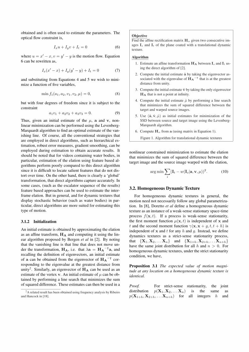
Objective

Find the affine rectification matrix Hα given two consecutive im-

ages Is and It of the plane coated with a translational dynamic

texture.

Algorithm

1. Estimate an affine transformation HA between Is and It us-

ing the direct algorithm of [2].

2. Compute the initial estimate a by taking the eigenvector as-

sociated with the eigenvalue of HA−⊺ that is at the greatest

distance from unity.

3. Compute the initial estimate v by taking the only eigenvector

HA that is not a point at infinity.

4. Compute the initial estimate µ by performing a line search

that minimizes the sum of squared difference between the

target and warped source images.

5. Use (a, v, µ) as initial estimates for minimization of the

SSD between source and target image using the Levenberg-

Marquardt algorithm.

6. Compute Hα from a (using matrix in Equation 1).

Figure 1. Algorithm for translational dynamic textures

nonlinear constrained minimization to estimate the elation

that minimizes the sum of squared difference between the

target image and the source image warped with the elation,

arg min∑

i

(It − w(Is|a,v, µ))2. (10)

3.2. Homogeneous Dynamic Texture

For homogeneous dynamic textures in general, the

motion need not necessarily follow any global parametriza-

tion. In [8], Doretto et al define a homogeneous dynamic

texture as an instance of a weak-sense stationary space-time

process f(x, t). If a process is weak-sense stationarity,

the first moment function µ(x, t) is independent of x and

t and the second moment function γ(x,x + g, t, t + h) is

independent of x and t for any h and g. Instead, we define

dynamics textures as a strict-sense stationarity process,

that {X1,X2, . . .Xn} and {X1+h,X2+h, . . .Xn+h}have the same joint distribution for all h and n > 0. For

homogeneous dynamic textures, under the strict stationarity

condition, we have,

Proposition 3.1 The expected value of motion magni-

tude at any location on a homogeneous dynamic texture is

identical.

Proof. For strict-sense stationarity, the joint

distribution p(X1,X2, . . .Xn) is the same as

p(X1+h,X2+h, . . .Xn+h) for all integers h and

n > 0. Therefore, for any function g(·), the distri-

bution of p(g(X1,X2, . . .Xn)) will be identical to

p(g(X1+h,X2+h, . . .Xn+h)). Since the brightness

constancy constraint equation is a function only of the

intensities of pixels, i.e. it uses spatial and temporal

gradients and does not use location for computation,

the distribution of flow and therefore the distribu-

tion of flow magnitude ρ(·) (a function, in turn, of

flow) will also be stationary. Therefore, the expected

value of motion magnitude E[p(ρ(X1,X2, . . .Xn))] =E[p(ρ(X1+h,X2+h, . . .Xn+h))] for all integers n > 0and h. It should be noted that since flow is estimated

locally, it is sufficient to require only that the joint distribu-

tion of local neighborhoods remain the same at any location.

Then, analogous to Gibson’s statement on texture gra-

dients, we have

Proposition 3.2 In perspective images of a plane with

a homogeneous dynamic texture, the gradient of imaged

motion magnitude is perpendicular to the vanishing line in

the image coordinate.

Proof. From Proposition 3.1, the expected value of

motion magnitude is equal all over the 3D world plane,

and thus when projected onto an image plane it captures

the perspective effects of image projection. Criminisi and

Zisserman provide a geometric proof that the gradient of

any perspective effect is perpendicular to the vanishing line

in [6].

3.2.1 Estimation of the Vanishing Line

We model the motion magnitude at a pixel as a univari-

ate Gaussian distribution, and sequentially estimate the ex-

pected value (mean) of motion magnitudes per pixel over

time, i.e. that the magnitude of motion at a pixel is dis-

tributed κ(i, j) ∼ N(µ(i, j), σ(i, j)). At the incidence of

each frame, pixel-wise optical flow is computed and used to

update the current estimates of µ and σ. To recover the van-

ishing line from the field of motion magnitudes, we need to

fit a line to the projections of points onto the x − y plane

(image coordinates) along the motion magnitude gradient

direction. This is equivalent to solving the following linear

system of equations,

Ya = s (11)

where

Y =

x1 y1 1x2 y2 1

...

xn yn 1

, s =

κ(x1, y1)κ(x2, y2)

...

κ(xn, yn)

(12)

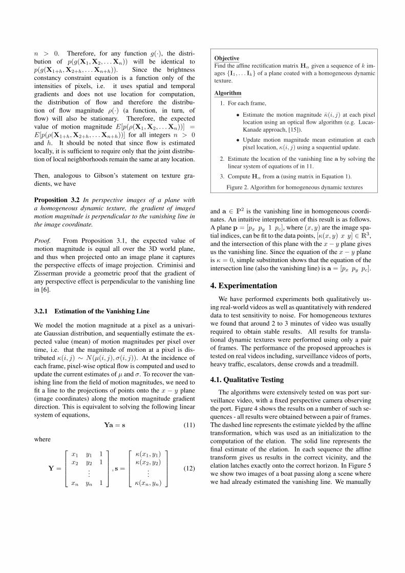
Objective

Find the affine rectification matrix Hα given a sequence of k im-

ages {I1, . . . Ik} of a plane coated with a homogeneous dynamic

texture.

Algorithm

1. For each frame,

• Estimate the motion magnitude κ(i, j) at each pixel

location using an optical flow algorithm (e.g. Lucas-

Kanade approach, [15]).

• Update motion magnitude mean estimation at each

pixel location, κ(i, j) using a sequential update.

2. Estimate the location of the vanishing line a by solving the

linear system of equations of in 11.

3. Compute Hα from a (using matrix in Equation 1).

Figure 2. Algorithm for homogeneous dynamic textures

and a ∈ P2 is the vanishing line in homogeneous coordi-

nates. An intuitive interpretation of this result is as follows.

A plane p = [px py 1 pc], where (x, y) are the image spa-

tial indices, can be fit to the data points, [κ(x, y) x y] ∈ R3,

and the intersection of this plane with the x− y plane gives

us the vanishing line. Since the equation of the x − y plane

is κ = 0, simple substitution shows that the equation of the

intersection line (also the vanishing line) is a = [px py pc].

4. Experimentation

We have performed experiments both qualitatively us-

ing real-world videos as well as quantitatively with rendered

data to test sensitivity to noise. For homogeneous textures

we found that around 2 to 3 minutes of video was usually

required to obtain stable results. All results for transla-

tional dynamic textures were performed using only a pair

of frames. The performance of the proposed approaches is

tested on real videos including, surveillance videos of ports,

heavy traffic, escalators, dense crowds and a treadmill.

4.1. Qualitative Testing

The algorithms were extensively tested on was port sur-

veillance video, with a fixed perspective camera observing

the port. Figure 4 shows the results on a number of such se-

quences - all results were obtained between a pair of frames.

The dashed line represents the estimate yielded by the affine

transformation, which was used as an initialization to the

computation of the elation. The solid line represents the

final estimate of the elation. In each sequence the affine

transform gives us results in the correct vicinity, and the

elation latches exactly onto the correct horizon. In Figure 5

we show two images of a boat passing along a scene where

we had already estimated the vanishing line. We manually

x−coordinate

y−

co

ord

ina

te

0 50 100 150 200 250 300

0

50

100

150

200

250

x−coordinate

y−

co

ord

ina

te

0 50 100 150 200 250 300

0

50

100

150

200

250

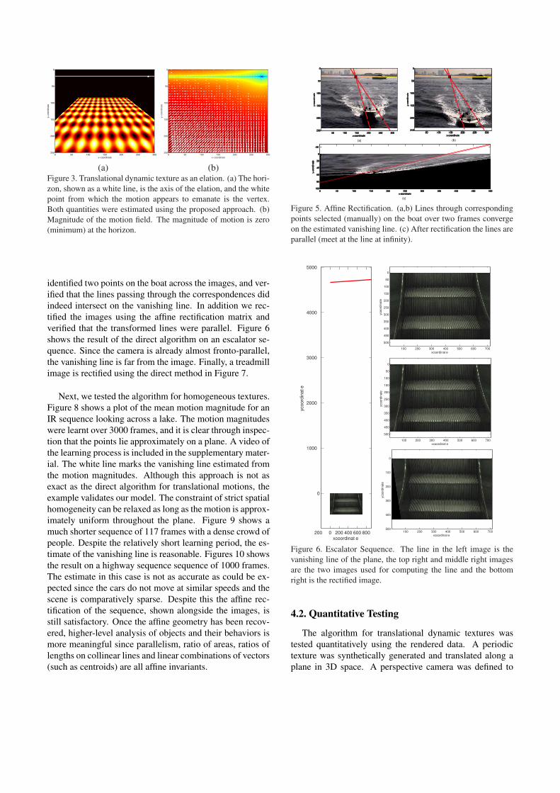
(a) (b)Figure 3. Translational dynamic texture as an elation. (a) The hori-

zon, shown as a white line, is the axis of the elation, and the white

point from which the motion appears to emanate is the vertex.

Both quantities were estimated using the proposed approach. (b)

Magnitude of the motion field. The magnitude of motion is zero

(minimum) at the horizon.

identified two points on the boat across the images, and ver-

ified that the lines passing through the correspondences did

indeed intersect on the vanishing line. In addition we rec-

tified the images using the affine rectification matrix and

verified that the transformed lines were parallel. Figure 6

shows the result of the direct algorithm on an escalator se-

quence. Since the camera is already almost fronto-parallel,

the vanishing line is far from the image. Finally, a treadmill

image is rectified using the direct method in Figure 7.

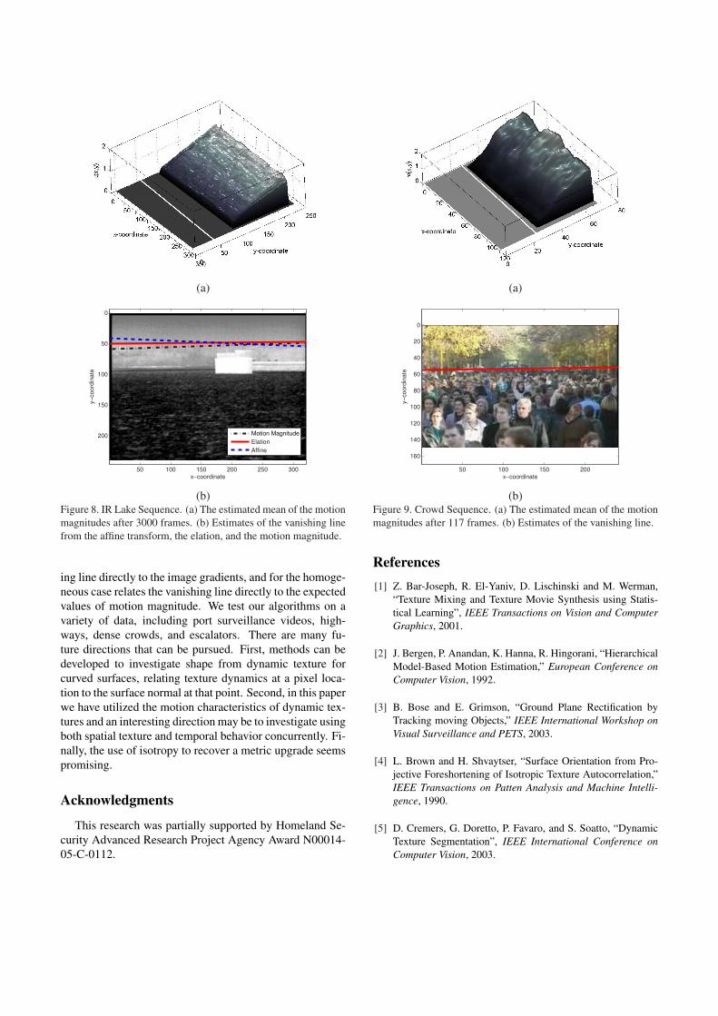
Next, we tested the algorithm for homogeneous textures.

Figure 8 shows a plot of the mean motion magnitude for an

IR sequence looking across a lake. The motion magnitudes

were learnt over 3000 frames, and it is clear through inspec-

tion that the points lie approximately on a plane. A video of

the learning process is included in the supplementary mater-

ial. The white line marks the vanishing line estimated from

the motion magnitudes. Although this approach is not as

exact as the direct algorithm for translational motions, the

example validates our model. The constraint of strict spatial

homogeneity can be relaxed as long as the motion is approx-

imately uniform throughout the plane. Figure 9 shows a

much shorter sequence of 117 frames with a dense crowd of

people. Despite the relatively short learning period, the es-

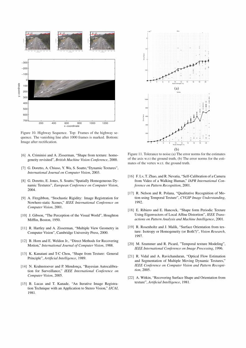
timate of the vanishing line is reasonable. Figures 10 shows

the result on a highway sequence sequence of 1000 frames.

The estimate in this case is not as accurate as could be ex-

pected since the cars do not move at similar speeds and the

scene is comparatively sparse. Despite this the affine rec-

tification of the sequence, shown alongside the images, is

still satisfactory. Once the affine geometry has been recov-

ered, higher-level analysis of objects and their behaviors is

more meaningful since parallelism, ratio of areas, ratios of

lengths on collinear lines and linear combinations of vectors

(such as centroids) are all affine invariants.

(a) (b)

(c)

Figure 5. Affine Rectification. (a,b) Lines through corresponding

points selected (manually) on the boat over two frames converge

on the estimated vanishing line. (c) After rectification the lines are

parallel (meet at the line at infinity).

x�coordinat e

y�coord

inat e

�200 0 200 400 600 800

�5000

�4000

�3000

�2000

�1000

0

x�coordinat e

y�co

ord

ina

te

100 200 300 400 500 600 700

0

100

200

300

400

500

x�coordinat e

y�co

ord

ina

te

100 200 300 400 500 600 700

0

50

100

150

200

250

300

350

400

450

500

x�coordinat e

y�co

ord

ina

te

100 200 300 400 500 600 700

0

50

100

150

200

250

300

350

400

450

500

Figure 6. Escalator Sequence. The line in the left image is the

vanishing line of the plane, the top right and middle right images

are the two images used for computing the line and the bottom

right is the rectified image.

4.2. Quantitative Testing

The algorithm for translational dynamic textures was

tested quantitatively using the rendered data. A periodic

texture was synthetically generated and translated along a

plane in 3D space. A perspective camera was defined to

x−coordinate

y−

co

ord

ina

te

50 100 150 200 250 300

0

50

100

150

200

x−coordinate

y−

co

ord

ina

te

50 100 150 200 250 300

0

50

100

150

200

x−coordinate

y−

co

ord

ina

te

50 100 150 200 250 300

0

50

100

150

200

x−coordinate

y−

co

ord

ina

te

50 100 150 200 250 300

0

50

100

150

200

x−coordinate

y−

co

ord

ina

te

50 100 150 200 250 300

0

50

100

150

200

x−coordinate

y−

co

ord

ina

te

50 100 150 200 250 300

0

50

100

150

200

x−coordinate

y−

co

ord

ina

te

50 100 150 200 250 300

0

50

100

150

200

x−coordinate

y−

co

ord

ina

te

50 100 150 200 250 300

0

50

100

150

200

x−coordinate

y−

co

ord

ina

te

50 100 150 200 250 300

0

50

100

150

200

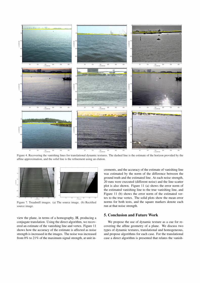
Figure 4. Recovering the vanishing lines for translational dynamic textures. The dashed line is the estimate of the horizon provided by the

affine approximation, and the solid line is the refinement using an elation.

x−coordinate

y−

co

ord

ina

te

0 50 100 150 200 250 300

50

100

150

200

250

x−coordinate

y−

co

ord

ina

te

50 100 150 200 250 300

0

50

100

150

200

Figure 7. Treadmill images. (a) The source image. (b) Rectified

source image.

view the plane, in terms of a homography, H, producing a

conjugate translation. Using the direct algorithm, we recov-

ered an estimate of the vanishing line and vertex. Figure 11

shows how the accuracy of the estimate is affected as noise

strength is increased in the images. The noise was increased

from 0% to 21% of the maximum signal strength, at unit in-

crements, and the accuracy of the estimate of vanishing line

was estimated by the norm of the difference between the

ground truth and the estimated line. At each noise strength,

20 runs were executed (different noise) and the line-scatter

plot is also shown. Figure 11 (a) shows the error norm of

the estimated vanishing line to the true vanishing line, and

Figure 11 (b) shows the error norm of the estimated ver-

tex to the true vertex. The solid plots show the mean error

norms for both tests, and the square markers denote each

run at that noise strength.

5. Conclusion and Future Work

We propose the use of dynamic texture as a cue for re-

covering the affine geometry of a plane. We discuss two

types of dynamic textures, translational and homogeneous,

and propose algorithms for each case. For the translational

case a direct algorithm is presented that relates the vanish-

(a)

x−coordinate

y−

co

ord

ina

te

50 100 150 200 250 300

0

50

100

150

200 Motion Magnitude

Elation

Affine

(b)Figure 8. IR Lake Sequence. (a) The estimated mean of the motion

magnitudes after 3000 frames. (b) Estimates of the vanishing line

from the affine transform, the elation, and the motion magnitude.

ing line directly to the image gradients, and for the homoge-

neous case relates the vanishing line directly to the expected

values of motion magnitude. We test our algorithms on a

variety of data, including port surveillance videos, high-

ways, dense crowds, and escalators. There are many fu-

ture directions that can be pursued. First, methods can be

developed to investigate shape from dynamic texture for

curved surfaces, relating texture dynamics at a pixel loca-

tion to the surface normal at that point. Second, in this paper

we have utilized the motion characteristics of dynamic tex-

tures and an interesting direction may be to investigate using

both spatial texture and temporal behavior concurrently. Fi-

nally, the use of isotropy to recover a metric upgrade seems

promising.

Acknowledgments

This research was partially supported by Homeland Se-

curity Advanced Research Project Agency Award N00014-

05-C-0112.

(a)

x−coordinate

y−

co

ord

ina

te

50 100 150 200

0

20

40

60

80

100

120

140

160

(b)Figure 9. Crowd Sequence. (a) The estimated mean of the motion

magnitudes after 117 frames. (b) Estimates of the vanishing line.

References

[1] Z. Bar-Joseph, R. El-Yaniv, D. Lischinski and M. Werman,

“Texture Mixing and Texture Movie Synthesis using Statis-

tical Learning”, IEEE Transactions on Vision and Computer

Graphics, 2001.

[2] J. Bergen, P. Anandan, K. Hanna, R. Hingorani, “Hierarchical

Model-Based Motion Estimation,” European Conference on

Computer Vision, 1992.

[3] B. Bose and E. Grimson, “Ground Plane Rectification by

Tracking moving Objects,” IEEE International Workshop on

Visual Surveillance and PETS, 2003.

[4] L. Brown and H. Shvaytser, “Surface Orientation from Pro-

jective Foreshortening of Isotropic Texture Autocorrelation,”

IEEE Transactions on Patten Analysis and Machine Intelli-

gence, 1990.

[5] D. Cremers, G. Doretto, P. Favaro, and S. Soatto, “Dynamic

Texture Segmentation”, IEEE International Conference on

Computer Vision, 2003.

x−coordinate

y−

coord

inate

20 40 60 80 100 120 140 160

0

20

40

60

80

100

120

x−coordinate

y−

coord

inate

20 40 60 80 100 120 140 160

0

20

40

60

80

100

120

x−coordinate

y−

coord

inate

20 40 60 80 100 120 140 160

0

20

40

60

80

100

120

x−coordinate

y−co

ord

inate

200 400 600 800 1000 1200

−300

−200

−100

0

100

200

300

400

500

600

700

Figure 10. Highway Sequence. Top: Frames of the highway se-

quence. The vanishing line after 1000 frames is marked. Bottom:

Image after rectification.

[6] A. Criminisi and A. Zisserman, “Shape from texture: homo-

geneity revisited”, British Machine Vision Conference, 2000.

[7] G. Doretto, A. Chiuso, Y. Wu, S. Soatto,“Dynamic Textures”,

International Journal on Computer Vision, 2003.

[8] G. Doretto, E. Jones, S. Soatto,“Spatially Homogeneous Dy-

namic Textures”, European Conference on Computer Vision,

2004.

[9] A. Fitzgibbon, “Stochastic Rigidity: Image Registration for

Nowhere-static Scenes,” IEEE International Conference on

Computer Vision, 2001.

[10] J. Gibson, “The Perception of the Visual World”, Houghton

Mifflin, Boston, 1950.

[11] R. Hartley and A. Zisserman, “Multiple View Geometry in

Computer Vision”, Cambridge University Press, 2000.

[12] B. Horn and E. Weldon Jr., “Direct Methods for Recovering

Motion,” International Journal of Computer Vision, 1988.

[13] K. Kanatani and T-C Chou, “Shape from Texture: General

Principle”, Artificial Intelligence, 1989.

[14] N. Krahnstoever and P. Mendonca, “Bayesian Autocalibra-

tion for Surveillance,” IEEE International Conference on

Computer Vision, 2005.

[15] B. Lucas and T. Kanade, “An Iterative Image Registra-

tion Technique with an Application to Stereo Vision,” IJCAI,

1981.

2 4 6 8 10 12 14 16 18 200

0.5

1

1.5

2

x 10−3

Noise Strength (%)

Err

or

No

rm

Axis

(a)

2 4 6 8 10 12 14 16 18 200

200

400

600

800

1000

Noise Strength (%)E

rror

Norm

Vertex

(b)Figure 11. Tolerance to noise.(a) The error norms for the estimates

of the axis w.r.t the ground truth, (b) The error norms for the esti-

mates of the vertex w.r.t. the ground truth.

[16] F. Lv, T. Zhao, and R. Nevatia, “Self-Calibration of a Camera

from Video of a Walking Human,” IAPR International Con-

ference on Pattern Recognition, 2001.

[17] R. Nelson and R. Polana, “Qualitative Recognition of Mo-

tion using Temporal Texture”, CVGIP Image Understanding,

1992.

[18] E. Ribiero and E. Hancock, “Shape form Periodic Texture

Using Eigenvectors of Local Affine Distortion”, IEEE Trans-

actions on Pattern Analysis and Machine Intelligence, 2001.

[19] R. Rosenholtz and J. Malik, “Surface Orientation from tex-

ture: Isotropy or Homogeneity (or Both?)”, Vision Research,

1997.

[20] M. Szummer and R. Picard, ”Temporal texture Modeling”,

IEEE International Conference on Image Processing, 1996.

[21] R. Vidal and A. Ravichandaran, “Optical Flow Estimation

and Segmentation of Multiple Moving Dynamic Textures,”

IEEE Conference on Computer Vision and Pattern Recogni-

tion, 2005.

[22] A. Witkin, “Recovering Surface Shape and Orientation from

texture”, Artificial Intelligence, 1981.