Embed Size (px)
Citation preview

SAS/STAT® 14.3User’s GuideShared Concepts andTopics

This document is an individual chapter from SAS/STAT® 14.3 User’s Guide.
The correct bibliographic citation for this manual is as follows: SAS Institute Inc. 2017. SAS/STAT® 14.3 User’s Guide. Cary, NC:SAS Institute Inc.
SAS/STAT® 14.3 User’s Guide
Copyright © 2017, SAS Institute Inc., Cary, NC, USA
All Rights Reserved. Produced in the United States of America.
For a hard-copy book: No part of this publication may be reproduced, stored in a retrieval system, or transmitted, in any form or byany means, electronic, mechanical, photocopying, or otherwise, without the prior written permission of the publisher, SAS InstituteInc.
For a web download or e-book: Your use of this publication shall be governed by the terms established by the vendor at the timeyou acquire this publication.
The scanning, uploading, and distribution of this book via the Internet or any other means without the permission of the publisher isillegal and punishable by law. Please purchase only authorized electronic editions and do not participate in or encourage electronicpiracy of copyrighted materials. Your support of others’ rights is appreciated.
U.S. Government License Rights; Restricted Rights: The Software and its documentation is commercial computer softwaredeveloped at private expense and is provided with RESTRICTED RIGHTS to the United States Government. Use, duplication, ordisclosure of the Software by the United States Government is subject to the license terms of this Agreement pursuant to, asapplicable, FAR 12.212, DFAR 227.7202-1(a), DFAR 227.7202-3(a), and DFAR 227.7202-4, and, to the extent required under U.S.federal law, the minimum restricted rights as set out in FAR 52.227-19 (DEC 2007). If FAR 52.227-19 is applicable, this provisionserves as notice under clause (c) thereof and no other notice is required to be affixed to the Software or documentation. TheGovernment’s rights in Software and documentation shall be only those set forth in this Agreement.
SAS Institute Inc., SAS Campus Drive, Cary, NC 27513-2414
September 2017
SAS® and all other SAS Institute Inc. product or service names are registered trademarks or trademarks of SAS Institute Inc. in theUSA and other countries. ® indicates USA registration.
Other brand and product names are trademarks of their respective companies.
SAS software may be provided with certain third-party software, including but not limited to open-source software, which islicensed under its applicable third-party software license agreement. For license information about third-party software distributedwith SAS software, refer to http://support.sas.com/thirdpartylicenses.

Chapter 19
Shared Concepts and Topics
ContentsLevelization of Classification Variables . . . . . . . . . . . . . . . . . . . . . . . . . . . . 388Parameterization of Model Effects . . . . . . . . . . . . . . . . . . . . . . . . . . . . . . . 391
GLM Parameterization of Classification Variables and Effects . . . . . . . . . . . . . 391Intercept . . . . . . . . . . . . . . . . . . . . . . . . . . . . . . . . . . . . . 391Regression Effects . . . . . . . . . . . . . . . . . . . . . . . . . . . . . . . 392Main Effects . . . . . . . . . . . . . . . . . . . . . . . . . . . . . . . . . . 392Interaction Effects . . . . . . . . . . . . . . . . . . . . . . . . . . . . . . . 392Nested Effects . . . . . . . . . . . . . . . . . . . . . . . . . . . . . . . . . . 393Continuous-Nesting-Class Effects . . . . . . . . . . . . . . . . . . . . . . . 393Continuous-by-Class Effects . . . . . . . . . . . . . . . . . . . . . . . . . . 394General Effects . . . . . . . . . . . . . . . . . . . . . . . . . . . . . . . . . 394
Other Parameterizations . . . . . . . . . . . . . . . . . . . . . . . . . . . . . . . . . 395CODE Statement . . . . . . . . . . . . . . . . . . . . . . . . . . . . . . . . . . . . . . . . 399
Syntax: CODE Statement . . . . . . . . . . . . . . . . . . . . . . . . . . . . . . . . 399EFFECT Statement . . . . . . . . . . . . . . . . . . . . . . . . . . . . . . . . . . . . . . . 401
Collection Effects . . . . . . . . . . . . . . . . . . . . . . . . . . . . . . . . . . . . 403Lag Effects . . . . . . . . . . . . . . . . . . . . . . . . . . . . . . . . . . . . . . . . 404Multimember Effects . . . . . . . . . . . . . . . . . . . . . . . . . . . . . . . . . . . 406Polynomial Effects . . . . . . . . . . . . . . . . . . . . . . . . . . . . . . . . . . . . 408Spline Effects . . . . . . . . . . . . . . . . . . . . . . . . . . . . . . . . . . . . . . 411Splines and Spline Bases . . . . . . . . . . . . . . . . . . . . . . . . . . . . . . . . . 415
Truncated Power Function Basis . . . . . . . . . . . . . . . . . . . . . . . . 416B-Spline Basis . . . . . . . . . . . . . . . . . . . . . . . . . . . . . . . . . 417Natural Cubic Spline Basis . . . . . . . . . . . . . . . . . . . . . . . . . . . 419
EFFECTPLOT Statement . . . . . . . . . . . . . . . . . . . . . . . . . . . . . . . . . . . . 420Syntax: EFFECTPLOT Statement . . . . . . . . . . . . . . . . . . . . . . . . . . . . 420
Dictionary of Options . . . . . . . . . . . . . . . . . . . . . . . . . . . . . . 422ODS Graphics: EFFECTPLOT Statement . . . . . . . . . . . . . . . . . . . . . . . . 431Examples: EFFECTPLOT Statement . . . . . . . . . . . . . . . . . . . . . . . . . . 432Example 19.1: A Saddle Surface . . . . . . . . . . . . . . . . . . . . . . . . . . . . . 432Example 19.2: Unbalanced Two-Way ANOVA . . . . . . . . . . . . . . . . . . . . . 436Example 19.3: Logistic Regression . . . . . . . . . . . . . . . . . . . . . . . . . . . 443
ESTIMATE Statement . . . . . . . . . . . . . . . . . . . . . . . . . . . . . . . . . . . . . 448Syntax: ESTIMATE Statement . . . . . . . . . . . . . . . . . . . . . . . . . . . . . 448Positional and Nonpositional Syntax for Coefficients in Linear Functions . . . . . . . 459

388 F Chapter 19: Shared Concepts and Topics
Joint Hypothesis Tests with Complex Alternatives, the Chi-Bar-Square Statistic . . . . 461ODS Table Names: ESTIMATE Statement . . . . . . . . . . . . . . . . . . . . . . . 462ODS Graphics: ESTIMATE Statement . . . . . . . . . . . . . . . . . . . . . . . . . 463
LSMEANS Statement . . . . . . . . . . . . . . . . . . . . . . . . . . . . . . . . . . . . . 464Syntax: LSMEANS Statement . . . . . . . . . . . . . . . . . . . . . . . . . . . . . . 465Construction of Least Squares Means . . . . . . . . . . . . . . . . . . . . . . . . . . 479
Setting Covariate Values . . . . . . . . . . . . . . . . . . . . . . . . . . . . 480Changing the Weighting Scheme . . . . . . . . . . . . . . . . . . . . . . . . 481Estimability of LS-Means . . . . . . . . . . . . . . . . . . . . . . . . . . . 482
ODS Table Names: LSMEANS Statement . . . . . . . . . . . . . . . . . . . . . . . 482ODS Graphics: LSMEANS Statement . . . . . . . . . . . . . . . . . . . . . . . . . 482
LSMESTIMATE Statement . . . . . . . . . . . . . . . . . . . . . . . . . . . . . . . . . . 484Syntax: LSMESTIMATE Statement . . . . . . . . . . . . . . . . . . . . . . . . . . . 485ODS Table Names: LSMESTIMATE Statement . . . . . . . . . . . . . . . . . . . . 494ODS Graphics: LSMESTIMATE Statement . . . . . . . . . . . . . . . . . . . . . . . 495
NLOPTIONS Statement . . . . . . . . . . . . . . . . . . . . . . . . . . . . . . . . . . . . 496Syntax: NLOPTIONS Statement . . . . . . . . . . . . . . . . . . . . . . . . . . . . 496Choosing an Optimization Algorithm . . . . . . . . . . . . . . . . . . . . . . . . . . 508
First- or Second-Order Algorithms . . . . . . . . . . . . . . . . . . . . . . . 508Algorithm Descriptions . . . . . . . . . . . . . . . . . . . . . . . . . . . . . 509
SLICE Statement . . . . . . . . . . . . . . . . . . . . . . . . . . . . . . . . . . . . . . . . 512Syntax: SLICE Statement . . . . . . . . . . . . . . . . . . . . . . . . . . . . . . . . 514ODS Table Names: SLICE Statement . . . . . . . . . . . . . . . . . . . . . . . . . . 515
STORE Statement . . . . . . . . . . . . . . . . . . . . . . . . . . . . . . . . . . . . . . . 515Syntax: STORE Statement . . . . . . . . . . . . . . . . . . . . . . . . . . . . . . . . 516
TEST Statement . . . . . . . . . . . . . . . . . . . . . . . . . . . . . . . . . . . . . . . . 517Syntax: TEST Statement . . . . . . . . . . . . . . . . . . . . . . . . . . . . . . . . . 517ODS Table Names: TEST Statement . . . . . . . . . . . . . . . . . . . . . . . . . . 518
Programming Statements . . . . . . . . . . . . . . . . . . . . . . . . . . . . . . . . . . . . 519Convergence Status . . . . . . . . . . . . . . . . . . . . . . . . . . . . . . . . . . . . . . . 521References . . . . . . . . . . . . . . . . . . . . . . . . . . . . . . . . . . . . . . . . . . . 523
This chapter introduces a number of concepts that are common to two or more SAS/STAT procedures. Mostsections display a listing of the procedures for which the shared topic is relevant.
Levelization of Classification VariablesA classification variable is a variable that enters the statistical analysis or model not through its values, butthrough its levels. The process of associating values of a variable with levels is termed levelization.
This section covers in particular procedures that support a CLASS statement for specifying classificationvariables. Some of the concepts discussed also apply to procedures that use different syntax to requestlevelization of variables (for example, the CLASS() expansion in the TRANSREG procedure).

Levelization of Classification Variables F 389
During the process of levelization, observations that share the same value are assigned to the same level. Themanner in which values are grouped can be affected by the inclusion of formats. The sort order of the levelscan be determined with the ORDER= option in the procedure statement. With the GENMOD, GLMSELECT,and LOGISTIC procedures, you can also control the sort order separately for each variable in the CLASSstatement.
Consider the data on nine observations in Table 19.1. The variable A is integer valued, and the variable Xis a continuous variable with a missing value for the fourth observation. The fourth and fifth columns ofTable 19.1 apply two different formats to the variable X.
Table 19.1 Example Data for Levelization
Obs A x FORMATx 3.0
FORMATx 3.1
1 2 1.09 1 1.12 2 1.13 1 1.13 2 1.27 1 1.34 3 . . .5 3 2.26 2 2.36 3 2.48 2 2.57 4 3.34 3 3.38 4 3.34 3 3.39 4 3.14 3 3.1
By default, levelization of the variables groups observations by the formatted value of the variable, exceptfor numerical variables for which no explicit format is provided. Numerical variables for which no explicitformat is provided are sorted by their internal value. The levelization of the four columns in table Table 19.1leads to the level assignment in Table 19.2.
Table 19.2 Values and Levels
A X FORMAT x 3.0 FORMAT x 3.1Obs Value Level Value Level Value Level Value Level
1 2 1 1.09 1 1 1 1.1 12 2 1 1.13 2 1 1 1.1 13 2 1 1.27 3 1 1 1.3 24 3 2 . . . . . .5 3 2 2.26 4 2 2 2.3 36 3 2 2.48 5 2 2 2.5 47 4 3 3.34 7 3 3 3.3 68 4 3 3.34 7 3 3 3.3 69 4 3 3.14 6 3 3 3.1 5
The ORDER= option in the PROC statement specifies the sort order for the levels of CLASS variables. WhenORDER=FORMATTED (which is the default) is in effect for numeric variables for which you have suppliedno explicit format, the levels are ordered by their internal values. To order numeric class levels with no

390 F Chapter 19: Shared Concepts and Topics
explicit format by their BEST12. formatted values, you can specify the BEST12. format explicitly for theCLASS variables.
The following table shows how values of the ORDER= option are interpreted.
Value of ORDER= Levels Sorted By
DATA Order of appearance in the input data set
FORMATTED External formatted value, except for numeric variables withno explicit format, which are sorted by their unformatted(internal) value
FREQ Descending frequency count; levels with the most observa-tions come first in the order
INTERNAL Unformatted value
For FORMATTED and INTERNAL values, the sort order is machine dependent. For more informationabout sort order, see the chapter on the SORT procedure in the SAS Visual Data Management and UtilityProcedures Guide and the discussion of BY-group processing in SAS Language Reference: Concepts.
The GLMSELECT, LOGISTIC, and GENMOD procedures support a MISSING option in the CLASSstatement. When this option is in effect, missing values (. for a numeric variable and blanks for a charactervariable) are included in the levelization and are assigned a level. Table 19.3 displays the results of levelizingthe values in Table 19.1 when the MISSING option is in effect.
Table 19.3 Values and Levels with MISSING Option
A X FORMAT x 3.0 FORMAT x 3.1Obs Value Level Value Level Value Level Value Level
1 2 1 1.09 2 1 2 1.1 22 2 1 1.13 3 1 2 1.1 23 2 1 1.27 4 1 2 1.3 34 3 2 . 1 . 1 . 15 3 2 2.26 5 2 3 2.3 46 3 2 2.48 6 2 3 2.5 57 4 3 3.34 8 3 4 3.3 78 4 3 3.34 8 3 4 3.3 79 4 3 3.14 7 3 4 3.1 6
When the MISSING option is not specified, or for procedures whose CLASS statement does not support thisoption, it is important to understand the implications of missing values for your statistical analysis. Whena SAS/STAT procedure levelizes the CLASS variables, an observation for which a CLASS variable has amissing value is excluded from the analysis. This is true regardless of whether the variable is used to formthe statistical model. Consider, for example, the case where some observations contain missing values forvariable A but the records for these observations are otherwise complete with respect to all other variables inthe statistical models. The analysis results from the following statements do not include any observations for

Parameterization of Model Effects F 391
which variable A contains missing values, even though A is not specified in the MODEL statement:
class A B;model y = B x B*x;
Many statistical procedures print a “Number of Observations” table that shows the number of observationsread from the data set and the number of observations used in the analysis. Pay careful attention to this table—especially when your data set contains missing values—to ensure that no observations are unintentionallyexcluded from the analysis.
Parameterization of Model EffectsThe general form of a linear regression model is defined in the section “Regression Models and Modelswith Classification Effects” on page 28 in Chapter 3, “Introduction to Statistical Modeling with SAS/STATSoftware,” as
Y D Xˇ C �
This section describes how matrices of regressor effects such as X are constructed in SAS/STAT software.These constructions (parameterization rules) apply to regression models, models with classification effects,generalized linear models, and mixed models. The simplest and most general parameterization rulesare the ones used in the GLM procedure, and they are discussed first. Several procedures also supportalternate parameterizations of classification variables, including the CATMOD, GENMOD, GLMSELECT,LOGISTIC, PHREG, SURVEYLOGISTIC, and SURVEYPHREG procedures. These are discussed after theGLM parameterization of classification variables and model effects.
All modeling procedures that have a CLASS statement support classification variables and effects, and thoseprocedures that additionally support the supplemental parameterizations have a PARAM= option in theCLASS statement.
GLM Parameterization of Classification Variables and Effects
This section applies to the following procedures:GAM, GENMOD, GLIMMIX, GLM, GLMPOWER, GLMSELECT, LIFEREG, LOGISTIC, MI, MIXED,MULLTEST, ORTHOREG, PHREG, PLS, QUANTREG, ROBUSTREG, SURVEYLOGISTIC, and SUR-VEYPHREG.
Intercept
By default, SAS/STAT linear models automatically include a column of 1s in X which corresponds to anintercept parameter. In many procedures you can use the NOINT option in the MODEL statement to suppressthis intercept. For example, the NOINT option is useful when the MODEL statement contains a classificationeffect and you want the parameter estimates to be in terms of the mean response for each level of that effect.
392 F Chapter 19: Shared Concepts and Topics
Regression Effects
Numeric variables or polynomial terms that involve them can be included in the model as regression effects(covariates). The actual values of such terms are included as columns of the relevant model matrices. Youcan use the bar operator with a regression effect to generate polynomial effects. For example, X|X|X expandsto X X*X X*X*X, which is a cubic model.
Main Effects
If a classification variable has m levels, the GLM parameterization generates m columns for its main effect inthe model matrix. Each column is an indicator variable for a given level. The order of the columns is the sortorder of the values of their levels and frequently can be controlled with the ORDER= option in the procedureor CLASS statement.
Table 19.4 is an example where ˇ0 denotes the intercept and A and B are classification variables with twoand three levels, respectively.
Table 19.4 Example of Main Effects
Data I A B
A B ˇ0 A1 A2 B1 B2 B31 1 1 1 0 1 0 01 2 1 1 0 0 1 01 3 1 1 0 0 0 12 1 1 0 1 1 0 02 2 1 0 1 0 1 02 3 1 0 1 0 0 1
Typically, there are more columns for these effects than there are degrees of freedom to estimate them. Inother words, the GLM parameterization of main effects is singular.
Interaction Effects
Often a model includes interaction (crossed) effects to account for how the effect of a variable changeswith the values of other variables. With an interaction, the terms are first reordered to correspond to theorder of the variables in the CLASS statement. Thus, B*A becomes A*B if A precedes B in the CLASSstatement. Then, the GLM parameterization generates columns for all combinations of levels that occur inthe data. The order of the columns is such that the rightmost variables in the interaction change faster thanthe leftmost variables (Table 19.5). In the MIXED and GLIMMIX procedures, which support both fixed-and random-effects models, empty columns (that is, columns that would contain all 0s) are not generated forfixed effects, but they are generated for random effects.
Table 19.5 Example of Interaction Effects
Data I A B A*B
A B ˇ0 A1 A2 B1 B2 B3 A1B1 A1B2 A1B3 A2B1 A2B2 A2B31 1 1 1 0 1 0 0 1 0 0 0 0 01 2 1 1 0 0 1 0 0 1 0 0 0 0

GLM Parameterization of Classification Variables and Effects F 393
Table 19.5 continued
Data I A B A*B
1 3 1 1 0 0 0 1 0 0 1 0 0 02 1 1 0 1 1 0 0 0 0 0 1 0 02 2 1 0 1 0 1 0 0 0 0 0 1 02 3 1 0 1 0 0 1 0 0 0 0 0 1
In the preceding matrix, main-effects columns are not linearly independent of crossed-effects columns; infact, the column space for the crossed effects contains the space of the main effect.
When your model contains many interaction effects, you might be able to code them more parsimoniously byusing the bar operator ( | ). The bar operator generates all possible interaction effects. For example, A|B|Cexpands to A B A*B C A*C B*C A*B*C. To eliminate higher-order interaction effects, use the at sign (@) inconjunction with the bar operator. For instance, A|B|C|D@2 expands to A B A*B C A*C B*C D A*D B*DC*D.
Nested Effects
Nested effects are generated in the same manner as crossed effects. Hence, the design columns generated bythe following two statements are the same (but the ordering of the columns is different):
model Y=A B(A);model Y=A A*B;
The nesting operator in SAS/STAT software is more of a notational convenience than an operation distinctfrom crossing. Nested effects are typically characterized by the property that the nested variables neverappear as main effects. The order of the variables within nesting parentheses is made to correspond to theorder of these variables in the CLASS statement. The order of the columns is such that variables outside theparentheses index faster than those inside the parentheses, and the rightmost nested variables index fasterthan the leftmost variables (Table 19.6).
Table 19.6 Example of Nested Effects
Data I A B(A)
A B ˇ0 A1 A2 B1A1 B2A1 B3A1 B1A2 B2A2 B3A21 1 1 1 0 1 0 0 0 0 01 2 1 1 0 0 1 0 0 0 01 3 1 1 0 0 0 1 0 0 02 1 1 0 1 0 0 0 1 0 02 2 1 0 1 0 0 0 0 1 02 3 1 0 1 0 0 0 0 0 1
Continuous-Nesting-Class Effects
When a continuous variable nests or crosses with a classification variable, the design columns are constructedby multiplying the continuous values into the design columns for the classification effect (Table 19.7).

394 F Chapter 19: Shared Concepts and Topics
Table 19.7 Example of Continuous-Nesting-Class Effects
Data I A X(A)
X A ˇ0 A1 A2 X(A1) X(A2)21 1 1 1 0 21 024 1 1 1 0 24 022 1 1 1 0 22 028 2 1 0 1 0 2819 2 1 0 1 0 1923 2 1 0 1 0 23
This model estimates a separate intercept and a separate slope for X within each level of A.
Continuous-by-Class Effects
Continuous-by-class effects generate the same design columns as continuous-nesting-class effects. Table 19.8shows the construction of the X*A effect. The two columns for this effect are the same as the columns for theX(A) effect in Table 19.7.
Table 19.8 Example of Continuous-by-Class Effects
Data I X A X*A
X A ˇ0 X A1 A2 X*A1 X*A221 1 1 21 1 0 21 024 1 1 24 1 0 24 022 1 1 22 1 0 22 028 2 1 28 0 1 0 2819 2 1 19 0 1 0 1923 2 1 23 0 1 0 23
You can use continuous-by-class effects together with pure continuous effects to test for homogeneity ofslopes.
General Effects
An example that combines all the effects is X1*X2*A*B*C(D E). The continuous list comes first, followedby the crossed list, followed by the nested list in parentheses. You should be aware of the sequencing ofparameters when you use statements that depend on the ordering of parameters. Such statements includeCONTRAST and ESTIMATE statements, which are used in a number of procedures to estimate and testfunctions of the parameters.
Effects might be renamed by the procedure to correspond to ordering rules. For example, B*A(E D) might berenamed A*B(D E) to satisfy the following:
� Classification variables that occur outside parentheses (crossed effects) are sorted in the order in whichthey appear in the CLASS statement.
Other Parameterizations F 395
� Variables within parentheses (nested effects) are sorted in the order in which they appear in the CLASSstatement.
The sequencing of the parameters generated by an effect can be described by which variables have theirlevels indexed faster:
� Variables in the crossed list index faster than variables in the nested list.
� Within a crossed or nested list, variables to the right index faster than variables to the left.
For example, suppose a model includes four effects—A, B, C, and D—each having two levels, 1 and 2. If theCLASS statement is
class A B C D;
then the order of the parameters for the effect B*A(C D), which is renamedA*B(C D), is
A1B1C1D1 ! A1B2C1D1 ! A2B1C1D1 ! A2B2C1D1 !
A1B1C1D2 ! A1B2C1D2 ! A2B1C1D2 ! A2B2C1D2 !
A1B1C2D1 ! A1B2C2D1 ! A2B1C2D1 ! A2B2C2D1 !
A1B1C2D2 ! A1B2C2D2 ! A2B1C2D2 ! A2B2C2D2
Note that first the crossed effects B and A are sorted in the order in which they appear in the CLASSstatement so that A precedes B in the parameter list. Then, for each combination of the nested effects in turn,combinations of A and B appear. The B effect changes fastest because it is rightmost in the cross list. Then Achanges next fastest, and D changes next fastest. The C effect changes most slowly because it is leftmost inthe nested list.
Other Parameterizations
This section applies to the following procedures:CATMOD, GENMOD, GLMSELECT, LOGISTIC, PHREG, and SURVEYPHREG.
Some SAS/STAT procedures, including GENMOD, GLMSELECT, and LOGISTIC, support nonsingularparameterizations for classification effects. A variety of these nonsingular parameterizations are avail-able. In most of these procedures you use the PARAM= option in the CLASS statement to specify theparameterization.
Consider a model with one CLASS variable A that has four levels, 1, 2, 5, and 7. Details of the possiblechoices for the PARAM= option follow.
EFFECT Three columns are created to indicate group membership of the nonreference levels.For the reference level, all three dummy variables have a value of –1. For example, ifthe reference level is 7 (REF=7), the design matrix columns for A are as follows.

396 F Chapter 19: Shared Concepts and Topics
Effect CodingDesign Matrix
A A1 A2 A5
1 1 0 02 0 1 05 0 0 17 –1 –1 –1
Parameter estimates of CLASS main effects that use the effect coding scheme estimatethe difference in the effect of each nonreference level compared to the average effectover all four levels.
The EFFECT parameterization is the default parameterization in the CATMODprocedure. See the section “Generation of the Design Matrix” on page 2005, inChapter 32, “The CATMOD Procedure,” for further details about parameterization ofmodel effects with the CATMOD procedure.
GLM As in the GLM procedure, four columns are created to indicate group membership.The design matrix columns for A are as follows.
GLM CodingDesign Matrix
A A1 A2 A5 A7
1 1 0 0 02 0 1 0 05 0 0 1 07 0 0 0 1
Parameter estimates of CLASS main effects that use the GLM coding scheme estimatethe difference in the effects of each level compared to the last level. See the previoussection for details about the GLM parameterization of model effects.
ORDINAL | THERMOMETER Three columns are created to indicate group membership of the higherlevels of the effect. For the first level of the effect (which for A is 1), all three dummyvariables have a value of 0. The design matrix columns for A are as follows.
Ordinal CodingDesign Matrix
A A2 A5 A7
1 0 0 02 1 0 05 1 1 07 1 1 1
The first level of the effect is a control or baseline level. Parameter estimates ofCLASS main effects, using the ORDINAL coding scheme, estimate the differences

Other Parameterizations F 397
between effects of successive levels. When the parameters have the same sign, theeffect is monotonic across the levels.
POLYNOMIAL | POLY Three columns are created. The first represents the linear term .x/, the secondrepresents the quadratic term
�x2�, and the third represents the cubic term
�x3�, where
x is the level value. If the CLASS levels are not numeric, they are translated into 1, 2,3, : : : according to their sort order. The design matrix columns for A are as follows.
Polynomial CodingDesign Matrix
A APOLY1 APOLY2 APOLY3
1 1 1 12 2 4 85 5 25 1257 7 49 343
REFERENCE | REF Three columns are created to indicate group membership of the nonreference levels.For the reference level, all three dummy variables have a value of 0. For example, ifthe reference level is 7 (REF=7), the design matrix columns for A are as follows.
Reference CodingDesign Matrix
A A1 A2 A5
1 1 0 02 0 1 05 0 0 17 0 0 0
Parameter estimates of CLASS main effects that use the reference coding schemeestimate the difference in the effect of each nonreference level compared to the effectof the reference level.The REFERENCE parameterization is also available through the MODEL statementin the CATMOD procedure. See the section “Generation of the Design Matrix” onpage 2005, in Chapter 32, “The CATMOD Procedure,” for further details aboutparameterization of model effects with the CATMOD procedure.
ORTHEFFECT The columns are obtained by applying the Gram-Schmidt orthogonalization to thecolumns for PARAM=EFFECT. The design matrix columns for A are as follows.
Orthogonal Effect CodingDesign Matrix
A AOEFF1 AOEFF2 AOEFF3
1 1.41421 –0.81650 –0.577352 0 1.63299 –0.577355 0 0 1.732057 –1.41421 –0.81649 –0.57735
398 F Chapter 19: Shared Concepts and Topics
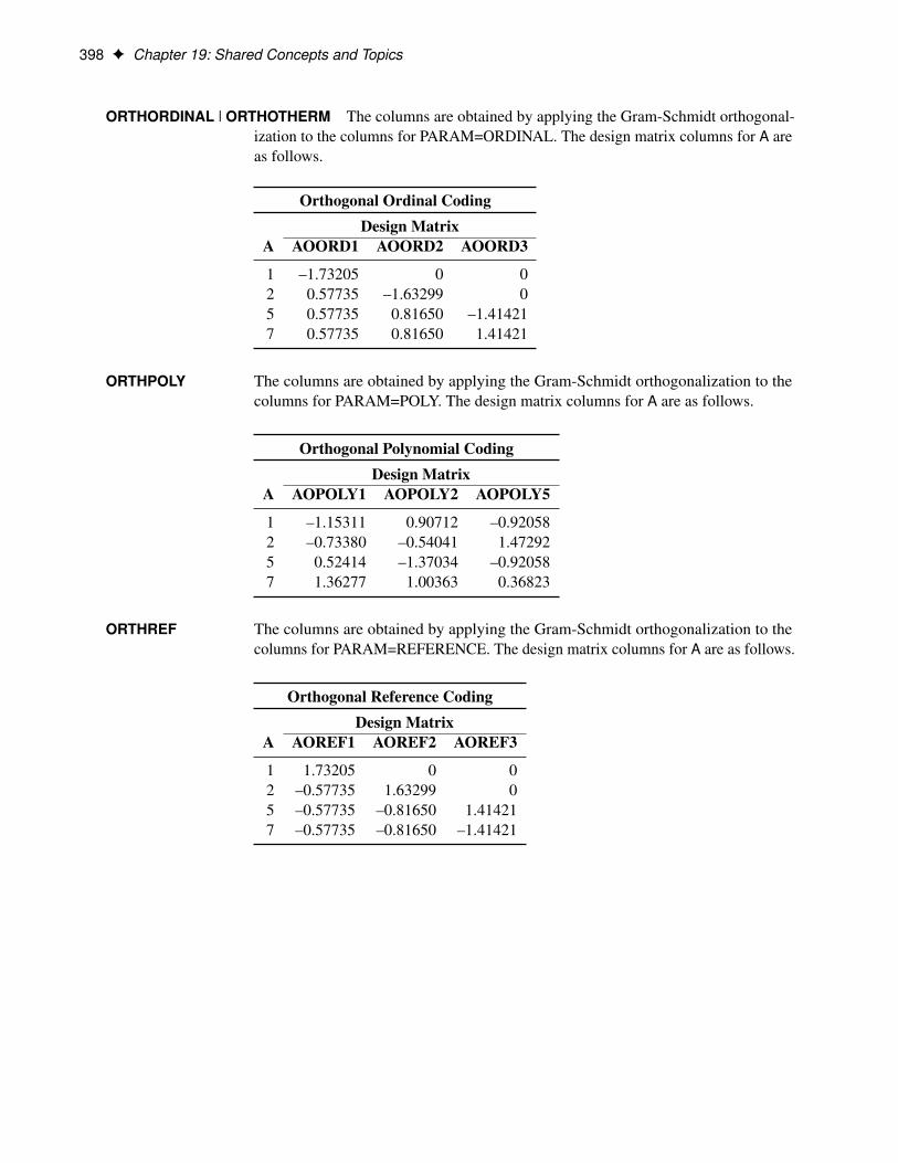
ORTHORDINAL | ORTHOTHERM The columns are obtained by applying the Gram-Schmidt orthogonal-ization to the columns for PARAM=ORDINAL. The design matrix columns for A areas follows.
Orthogonal Ordinal CodingDesign Matrix
A AOORD1 AOORD2 AOORD3
1 –1.73205 0 02 0.57735 –1.63299 05 0.57735 0.81650 –1.414217 0.57735 0.81650 1.41421
ORTHPOLY The columns are obtained by applying the Gram-Schmidt orthogonalization to thecolumns for PARAM=POLY. The design matrix columns for A are as follows.
Orthogonal Polynomial CodingDesign Matrix
A AOPOLY1 AOPOLY2 AOPOLY5
1 –1.15311 0.90712 –0.920582 –0.73380 –0.54041 1.472925 0.52414 –1.37034 –0.920587 1.36277 1.00363 0.36823
ORTHREF The columns are obtained by applying the Gram-Schmidt orthogonalization to thecolumns for PARAM=REFERENCE. The design matrix columns for A are as follows.
Orthogonal Reference CodingDesign Matrix
A AOREF1 AOREF2 AOREF3
1 1.73205 0 02 –0.57735 1.63299 05 –0.57735 –0.81650 1.414217 –0.57735 –0.81650 –1.41421

CODE Statement F 399
CODE Statement
This statement documentation applies to the following procedures:GENMOD, GLIMMIX, GLM, GLMSELECT, LOGISTIC, MIXED, PLM, and REG. It also applies to theHPLOGISTIC and HPREG procedures in SAS High-Performance Analytics software.
The CODE statement enables you to write SAS DATA step code to a file or catalog entry for computingpredicted values of the fitted model. This code can then be included in a DATA step to score new data.For example, in the following program, the CODE statement writes the code for predicting the outcomeof a logistic model to the file mycode.sas. The file is subsequently included in a DATA step to score thesashelp.Bmt data.
proc logistic data=sashelp.Bmt;class Group;model Status=Group;code file='mycode.sas';
run;
data Score;set sashelp.Bmt;%include mycode;
run;
Syntax: CODE StatementCODE < options > ;
Table 19.9 summarizes the options you can specify in the CODE statement.
Table 19.9 CODE Statement Options
Option Description
CATALOG= Names the catalog entry where the generated code is savedDUMMIES Retains the dummy variables in the data setERROR Computes the error functionFILE= Names the file where the generated code is savedFORMAT= Specifies the numeric format for the regression coefficientsGROUP= Specifies the group identifier for array names and statement labelsIMPUTE Imputes predicted values for observations with missing or invalid
covariatesLINESIZE= Specifies the line size of the generated codeLOOKUP= Specifies the algorithm for looking up CLASS levelsRESIDUAL Computes residuals

400 F Chapter 19: Shared Concepts and Topics
You cannot specify both the FILE= and CATALOG= options. If you specify neither, the SAS scoring code iswritten to the SAS log. You can specify the following options in the CODE statement.
CATALOG=library.catalog.entry.type
CAT=library.catalog.entry.typespecifies where to write the generated code in the form of library.catalog.entry.type. The compoundname can have from one to four levels. The default library is determined by the USER= SAS systemoption, which by default is WORK. The default entry is SASCODE, and the default type is SOURCE.
DUMMIES | NODUMMIESspecifies whether to keep dummy variables that represent the CLASS levels in the data set. The defaultis NODUMMIES, which specifies that dummy variables not be retained.
ERROR | NOERRORspecifies whether to generate code to compute the error function. The default is NOERROR, whichspecifies that the error function not be generated.
FILE=filenamenames the external file that saves the generated code. When enclosed in a quoted string (for example,FILE="c:nmydirnscorecode.sas"), this option specifies the path for writing the code to an externalfile. You can also specify unquoted SAS filenames of no more than eight characters for filename. Ifthe filename is assigned as a fileref in a Base SAS FILENAME statement, the file specified in theFILENAME statement is opened. The special filerefs LOG and PRINT are always assigned. If thespecified filename is not an assigned fileref , the specified value for filename is concatenated with a .txtextension before the file is opened. For example, if FOO is not an assigned fileref , FILE=FOO causesFOO.txt to be opened. If filename has more than eight characters, an error message is printed.
FORMAT=formatspecifies the format for the regression coefficients and other numerical values that do not have a formatfrom the input data set. The default format is BEST20.
GROUP=group-namespecifies the group identifier for group processing. The group-name should be a valid SAS name of nomore than 16 characters. It is used to construct array names and statement labels in the generated code.
IMPUTEimputes the predicted values according to an intercept-only model for observations with missing orinvalid covariate values. For a continuous response, the predicted value is the mean of the responsevariable; for a categorical response, the predicted values are the proportions of the response categories.When the IMPUTE option is specified, the scoring code also creates a variable named _WARN_ thatcontains one or more single-character codes that indicate problems in computing predicted values. Thecharacter codes used in _WARN_ go in the following positions:
Table 19.10 _WARN_ Variable Codes
Code Column Meaning
M 1 Missing covariate valueU 2 Unrecognized covariate category

EFFECT Statement F 401
LINESIZE=value
LS=valuespecifies the line size for the generated code. The default is 78. The permissible range is 78 to 254.
LOOKUP=lookup-methodspecifies the algorithm for looking up CLASS levels. You can specify the following lookup-methods:
AUTOselects the LINEAR algorithm if a CLASS variable has fewer than five categories; otherwise, theBINARY algorithm is used. This is the default.
BINARYuses a binary search. This method is fast, but might produce incorrect results and the normalizedcategory values might contain characters that collate in different orders in ASCII and EBCDIC,if you generate the code on an ASCII machine and execute the code on an EBCDIC machine orvice versa.
LINEARuses a linear search with IF statements that have categories in the order of the class levels. Thismethod is slow if there are many categories.
SELECTuses a SELECT statement.
The default is LOOKUP=AUTO.
RESIDUAL | NORESIDUALspecifies whether to generate code to compute residual values. If you request code for residuals andthen score a data set that does not contain target values, the residuals will have missing values. Thedefault is NORESIDUAL, which specifies that the code for residuals not be generated.
EFFECT Statement
This section applies to the following procedures:GLIMMIX, GLMSELECT, HPMIXED, LOGISTIC, ORTHOREG, PHREG, PLS, QUANTLIFE,QUANTREG, QUANTSELECT, ROBUSTREG, SURVEYLOGISTIC, and SURVEYREG.
The EFFECT statement enables you to construct special collections of columns for design matrices. Thesecollections are referred to as constructed effects to distinguish them from the usual model effects that areformed from continuous or classification variables, as discussed in the section “GLM Parameterization ofClassification Variables and Effects” on page 391. For example, the terms A, B, x, A*x, A*B, and sub in thefollowing statements define fixed, random, and subject effects of the usual type in a mixed model:
402 F Chapter 19: Shared Concepts and Topics
proc glimmix;class A B sub;model y = A B x A*x;random A*B / subject=sub;
run;
A constructed effect, on the other hand, is assigned through the EFFECT statement. For example, in thefollowing program, the EFFECT statement defines a constructed effect named spl:
proc glimmix;class A B SUB;effect spl = spline(x);model y = A B A*spl;random A*B / subject=sub;
run;
The columns of spl are formed from the data set variable x as a cubic B-spline basis with three equally spacedinterior knots.
Each constructed effect corresponds to a collection of columns that are referred to by using the name yousupply. You can specify multiple EFFECT statements, and all EFFECT statements must precede the MODELstatement.
The general syntax for the EFFECT statement with effect-specification is
EFFECT effect-name = effect-type (var-list < / effect-options >) ;
The name of the effect is specified after the EFFECT keyword. This name can appear in only one EFFECTstatement and cannot be the name of a variable in the input data set. The effect-type is specified after anequal sign, followed by a list of variables within parentheses which are used in constructing the effect.Effect-options that are specific to an effect-type can be specified after a slash (/) following the variable list.The following effect-types are available and are discussed in the following sections:
COLLECTION specifies a collection effect that defines one or more variables as a singleeffect with multiple degrees of freedom. The variables in a collection areconsidered as a unit for estimation and inference.
LAG specifies a classification effect in which the level that is used for a particularperiod corresponds to the level in the preceding period.
MULTIMEMBER | MM specifies a multimember classification effect whose levels are determined byone or more variables that appear in a CLASS statement.
POLYNOMIAL | POLY specifies a multivariate polynomial effect in the specified numeric variables.
SPLINE specifies a regression spline effect whose columns are univariate spline ex-pansions of one or more variables. A spline expansion replaces the originalvariable with an expanded or larger set of new variables.
Table 19.11 summarizes the options available in the EFFECT statement.

Collection Effects F 403
Table 19.11 EFFECT Statement Options
Option Description
Collection Effects OptionsDETAILS Displays the constituents of the collection effect
Lag Effects OptionsDESIGNROLE= Names a variable that controls to which lag design an observation
is assigned
DETAILS Displays the lag design of the lag effect
NLAG= Specifies the number of periods in the lag
PERIOD= Names the variable that defines the period. This option is required.
WITHIN= Names the variable or variables that define the group within whicheach period is defined. This option is required.
Multimember Effects OptionsNOEFFECT Specifies that observations with all missing levels for the
multimember variables should have zero values in thecorresponding design matrix columns
WEIGHT= Specifies the weight variable for the contributions of each of theclassification effects
Polynomial Effects OptionsDEGREE= Specifies the degree of the polynomialMDEGREE= Specifies the maximum degree of any variable in a term of the
polynomialSTANDARDIZE= Specifies centering and scaling suboptions for the variables that
define the polynomial
Spline Effects OptionsBASIS= Specifies the type of basis (B-spline basis or truncated power
function basis) for the spline effectDEGREE= Specifies the degree of the spline effectKNOTMETHOD= Specifies how to construct the knots for the spline effect
Collection EffectsEFFECT name=COLLECTION (var-list < / DETAILS >) ;
You use a collection effect to define a set of variables that are treated as a single effect with multiple degreesof freedom. The variables in var-list can be continuous or classification variables. The columns in the designmatrix that are contributed by a collection effect are the design columns of its constituent variables in theorder in which they appear in the definition of the collection effect. If you specify the DETAILS option, thena table that shows the constituents of the collection effect is displayed.

404 F Chapter 19: Shared Concepts and Topics
Lag EffectsEFFECT name=LAG (variable / WITHIN=variable PERIOD=variable lag-options) ;
EFFECT name=LAG (variable / WITHIN=(var-list) PERIOD=variable lag-options) ;
A lag effect is a classification effect for the variable that is specified after the keyword LAG. A lag effectrepresents the effect of a previous value of the lagged variable when the observations of this variable areinherently ordered. A typical example where lag effects are useful is a study in which different subjects aregiven sequences of treatments and you want to investigate whether the treatment in the previous period isimportant in understanding the outcome in the current period. You can do this by including a lagged treatmenteffect in your model.
The precise definition of a lag effect depends on a subdivision of the data into disjoint subsets and an orderinginto units of the observations within a subset. The subsets are often called subjects, and they are specifiedin the required WITHIN= option. The units are often called periods, and they are specified in the requiredPERIOD= option. For an observation that belongs to a particular subject at a particular period, the designmatrix columns of the lagged variable are the usual design matrix columns of that variable except for theobservation at the preceding period for that subject. Observations at the initial period do not have a precedingvalue, and so the design matrix columns of the lag effect for these observations are set to 0. You can alsodefine lag effects where the number of periods that are lagged is greater than 1. If the number of periods thatare lagged is n, then the design matrix columns of observations in periods less than or equal to n are set to 0.The design matrix columns that correspond to a subject at period p, where p > n, are the usual design matrixcolumns of the lagged variable for that subject at period p – n.
In a valid lag design there is at most one observation for a particular period and subject. For example, thefollowing set of treatments by subject and period form a valid lag design:
Subject Period Treatment
Sheila 1 BJoey 1 AAthena 1 AGelindo 1 ASheila 2 CJoey 2 AAthena 2 .Gelindo 2 BSheila 3 BJoey 3 CAthena 3 AGelindo 3 B
A convenient way to represent the organization of observations into subjects and periods is to form the lagdesign matrix. The rows and columns of this matrix correspond to the subjects and periods, respectively. Thelag design matrix entry is the treatment for the corresponding subject and period.

Lag Effects F 405
The associated lag design matrix is
PeriodSubject 1 2 3
Athena A AGelindo A B BJoey A A CSheila B C B
Note that the subject Athena did not receive a treatment at period 2, and so the corresponding entry in the lagdesign matrix is missing. The following statements define a lag effect for this lag design:
CLASS treatment;EFFECT Lag = LAG( treatment / WITHIN=subject PERIOD=period);
When GLM coding is used for the variable treatment, the design matrix columns Lag_A, Lag_B, and Lag_Cfor the constructed effect Lag are as follows:
Subject Period Treatment Lag_A Lag_B Lag_C
Athena 1 A 0 0 0Athena 2 1 0 0Athena 3 A . . .Gelindo 1 A 0 0 0Gelindo 2 B 1 0 0Gelindo 3 B 0 1 0Joey 1 A 0 0 0Joey 2 A 1 0 0Joey 3 C 1 0 0Sheila 1 B 0 0 0Sheila 2 C 0 1 0Sheila 3 B 0 0 1
The design matrix columns for each subject at period 1 are all 0 because there are no lagged observations forperiod 1. You can also see that the design matrix columns at period 3 for subject Athena are missing becauseAthena did not receive a treatment at period 2. Nevertheless, the design matrix columns for Athena at period2 are nonmissing and correspond to the treatment “A” that she received in period 1.
You must specify the following required options:
PERIOD=variablespecifies the period variable of the lag design. The number of periods is the number of unique formattedvalues of the variable, and the ordering of the period is formed by sorting these formatted values inascending order. You must specify this option.

406 F Chapter 19: Shared Concepts and Topics
WITHIN=(var-list) | variablespecifies a variable (or a list of variables within parentheses) that defines the subject grouping of thelag design. If there is only one WITHIN= variable, then the parentheses are not required. Each subjectis defined by the unique set of formatted values of the variables in the WITHIN= list. The subjects aresorted in ascending lexicographic order. You must specify this option.
You can also specify the following optional lag-options:
DESIGNROLE=variablespecifies a numeric variable that subsets observations into two groups: a group in which the value ofvariable is nonzero and a group in which the value of variable is zero. The observations in the firstgroup are used to form the lag design matrix that is used in fitting the model. The lag design thatcorresponds to the second group is used when observations in the input data set that do not belong tothe first group are scored. This option is useful when you want to obtain predicted values in an outputdata set for observations that are not used in fitting the model. If you do not specify this option, thenall observations are assigned to the first group.
DETAILSrequests a table that shows the lag design matrix of the lag effect.
NLAG=nspecifies the number of lags. By default NLAG=1.
Multimember EffectsEFFECT name=MULTIMEMBER (var-list < / mm-options >) ;
EFFECT name=MM (var-list < / mm-options >) ;
A multimember effect is formed from one or more classification variables in such a way that each observationcan be associated with one or more levels of the union of the levels of the classification variables. In otherwords, a multimember effect is a classification-type effect with possibly more than one nonzero column entryfor each observation. Multimember effects are useful, for example, in modeling the following:
� nurses’ effects on patient recovery in hospitals
� teachers’ effects on student scores
� lineage effects in genetic studies. See Example 47.16 in Chapter 47, “The GLIMMIX Procedure,” foran application with random multimember effects in a genetic diallel experiment.
The levels of a multimember effect consist of the union of formatted values of the variables that define thiseffect. Each such level contributes one column to the design matrix. For each observation, the value thatcorresponds to each level of the multimember effect in the design matrix is the number of times that this leveloccurs for the observation.
For example, the following data provide teacher information and end-of-year test scores for students aftertwo semesters:

Multimember Effects F 407
Student Score Teacher1 Teacher2
Mary 87 Tobias CohenTom 89 Rodriguez TobiasFred 82 Cohen CohenJane 88 Tobias .Jack 99 . .
For example, Mary had different teachers in the two semesters, Fred had the same teacher in both semesters,and Jane received instruction only in the first semester.
You can model the effect of the teachers on student performance by using a multimember effect specified asfollows:
CLASS teacher1 teacher2;EFFECT teacher = MM(teacher1 teacher2);
The levels of the teacher effect are Cohen, Rodriguez, and Tobias, and the associated design matrix columnsare as follows:
Student Cohen Rodriguez Tobias
Mary 1 0 1Tom 0 1 1Fred 2 0 0Jane 0 0 1Jack . . .
You can specify the following mm-options after a slash (/):
DETAILSrequests a table that shows the levels of the multimember effect.
NOEFFECTspecifies that, for observations with all missing levels of the multimember variables, the values in thecorresponding design matrix columns be set to zero. If, in the preceding example, the teacher effect isdefined by
EFFECT teacher = MM(teacher1 teacher2 / noeffect);
then the associated design matrix columns’ values for Jack are all zero. This enables you to includeJack in the analysis even though there is no effect of teachers on his performance.
A situation where it is important to designate observations as having no effect due to a classificationvariable is the analysis of crossover designs, where lagged treatment levels are used to model thecarryover effects of treatments between periods. Since there is no carryover effect for the first period,the treatment lag effect in a crossover design can be modeled with a multimember effect that consistsof a single classification variable and the NOEFFECT option, as in the following statements:

408 F Chapter 19: Shared Concepts and Topics
CLASS Treatment lagTreatment;EFFECT Carryover = MM(lagTreatment / noeffect);
The lagTreatment variable contains a missing value for the first period. Otherwise, it contains the valueof the treatment variable for the preceding period.
STDIZEspecifies that for each observation, the entries in the design matrix that corresponds to the multimembereffect be scaled to have a sum of one.
WEIGHT=wght-listspecifies numeric variables used to weigh the contributions of each of the classification effects thatdefine the constructed multimember effect. The number of variables in wght-list must match thenumber of classification variables that define the effect.
Polynomial EffectsEFFECT name=POLYNOMIAL (var-list < / polynomial-options >) ;
EFFECT name=POLY (var-list < / polynomial-options >) ;
The variables in var-list must be numeric. A design matrix column is generated for each term of the specifiedpolynomial. By default, each of these terms is treated as a separate effect for the purpose of model building.For example, the statements
proc glmselect;effect MyPoly = polynomial(x1-x3/degree=2);model y = MyPoly;
run;
yield the identical analysis to the statements
proc glmselect;model y = x1 x2 x3 x1*x1 x1*x2 x1*x3 x2*x2 x2*x3 x3*x3;
run;
You can specify the following polynomial-options after a slash (/):
DEGREE=nspecifies the degree of the polynomial. The degree must be a positive integer. The degree is typically asmall integer, such as 1, 2, or 3. The default is DEGREE=1.
DETAILSrequests a table that shows the details of the specified polynomial, including the number of termsgenerated. If you also specify the STANDARDIZE option, then a table that shows the standardizationdetails is also produced.
LABELSTYLE=(style-opts)LABELSTYLE=style-opt
specifies how the terms in the polynomial are labeled. By default, powers are shown with ˆ as theexponentiation operator and * as the multiplication operator. For example, a polynomial term such asx3
1x2x23 is labeled x1ˆ3*x2*x3ˆ2. You can change the style of the label by using the following style-opts
within parentheses. If you specify a single style-opt , then you can omit the enclosing parentheses.

Polynomial Effects F 409
EXPANDspecifies that each variable with an exponent greater than 1 be written as products of that variable.For example, the term x3
1x2x23 receives the label x1*x1*x1*x2*x3*x3.
EXPONENT < =quoted string >specifies that each variable with an exponent greater than 1 be written using exponential notation.By default, the symbol ˆ is used as the exponentiation operator. If you supply the optional quotedstring after an equal sign, then that string is used as the exponentiation operator. For example, ifyou specify
LABELSTYLE=(EXPONENT="**")
then the term x31x2x
23 receives the label x1**3*x2*x3**2.
INCLUDENAMEspecifies that the name of the effect followed by an underscore be used as a prefix for term labels.For example, the following statement generates terms with labels MyPoly_x1 and MyPoly_x1ˆ2:
EFFECT MyPoly=POLYNOMIAL(x1/degree=2 labelstyle=INCLUDENAME)
The INCLUDENAME option is ignored if you also specify the NOSEPARATE option in theEFFECT=POLYNOMIAL statement.
PRODUCTSYMBOL=NONE | quoted stringspecifies that the supplied string be used as the product symbol. For example, the followingstatement generates terms with labels x1, x2, and x1 x2:
EFFECT MyPoly=POLYNOMIAL(x1 x2 / degree=2 mdegree=1labelstyle=(PRODUCTSYMBOL=" "))
If you specify PRODUCTSYMBOL=NONE, then the labels are formed by juxtaposing theconstituent variable names.
MDEGREE=nspecifies the maximum degree of any variable in a term of the polynomial. This degree must be apositive integer. The default is the degree of the specified polynomial. For example, the followingstatement generates the terms x1, x2, x2
1 , x1x2, x22 , x2
1x2, x1x22 and x2
1x22 :
EFFECT MyPoly=POLYNOMIAL(x1 x2/degree=4 MDEGREE=2);
NOSEPARATEspecifies that the polynomial be treated as a single effect with multiple degrees of freedom. The effectname that you specify is used as the constructed effect name, and the labels of the terms are used aslabels of the corresponding parameters.

410 F Chapter 19: Shared Concepts and Topics
STANDARDIZE < (centerscale-opts) > < = standardize-opt >specifies that the variables that define the polynomial be standardized. By default, the standardizedvariables receive prefix “s_” in the variable names.
You can use the following centerscale-opts to specify how the center and scale are estimated:
METHOD=MOMENTSspecifies that the center be estimated by the variable mean and the scale be estimated by thestandard deviation. If a weight variable is specified using a WEIGHT statement, the observationswith invalid weights are ignored when forming the mean and standard deviation, but the weightsare otherwise not used. Only observations that are used in performing the analysis are used forthe standardization.
METHOD=RANGEspecifies that the center be estimated by the midpoint of the variable range and the scale beestimated as half the variable range. Any observation that has a missing value for any regressorused in the model is ignored when computing the range of variables in a polynomial effect.Observations with valid regressor values but missing or invalid values of frequency variables,weight variables, or dependent variables are used in computing variable ranges. The default (ifyou do not specify the METHOD= suboption) is METHOD=RANGE.
METHOD=WMOMENTSis the same as METHOD=MOMENTS except that weighted means and weighted standarddeviations are used.
Let
n D number of observations used in the analysisw D weight variablef D frequency variablex D variable to be standardized
x.n/ D MaxniD1.xi /
x.1/ D MinniD1.xi /
F D sum of frequenciesD †n
iD1fi
WF D sum of weighted frequenciesD †n
iD1wifi
Table 19.12 shows how the center and scale are computed for each of the supported methods.

Spline Effects F 411
Table 19.12 Center and Scale Estimates by Method
Method Center Scale
Range .x.n/ C x.1//=2 .x.n/ � x.1//=2
Moments Nx D †niD1fixi=F
q†n
iD1fi .xi � Nx/2=.F � 1/
WMoments Nxw D †niD1wifixi=WF
q†n
iD1wifi .xi � Nxw/2=.F � 1/
PREFIX=NONE | quoted-stringspecifies the prefix that is appended to standardized variables when forming the term labels. Ifyou omit this option, the default prefix is “s_”. If you specify PREFIX=NONE, then standardizedvariables are not prefixed.
You can control whether the standardization is to center, scale, or both center and scale by specifying astandardize-opt:
CENTERspecifies that variables be centered but not scaled. For a variable x,
s_x D x � center
CENTERSCALEspecifies that variables be centered and scaled. This is the default if you do not specify astandardization-opt . For a variable x,
s_x Dx � center
scale
NONEspecifies that no standardization be performed.
SCALEspecifies that variables be scaled but not centered. For a variable x,
s_x Dx
scale
Spline EffectsThis section discusses the construction of spline effects through the EFFECT statement. You can also includespline effects in statistical models by other means. The TRANSREG procedure has dedicated facilities forincluding regression splines in your model and controlling the construction of the splines. For example, youcan use the TRANSREG procedure to fit a spline function but restrict the function to be always increasingor decreasing (monotone). See the section “Using Splines and Knots” on page 9932 in Chapter 120, “TheTRANSREG Procedure,” for more information about using splines with the TRANSREG procedure. The
412 F Chapter 19: Shared Concepts and Topics
GAM and TPSPLINE procedures also can model the effects of regressor variables in terms of smoothfunctions that are generated from spline bases. For more information see Chapter 43, “The GAM Procedure,”and Chapter 119, “The TPSPLINE Procedure.”
A spline effect expands variables into spline bases whose form depends on the options that you specify.You can find details about regression splines and spline bases in the section “Splines and Spline Bases” onpage 415. You request a spline effect with the syntax
EFFECT name=SPLINE (var-list < / spline-options >) ;
The variables in var-list must be numeric. Design matrix columns are generated separately for each of thesevariables, and the set of columns is collectively referred to with the specified name. By default, the splinebasis that is generated for each variable is a cubic B-spline basis with three equally spaced knots positionedbetween the minimum and maximum values of that variable. This yields by default seven design matrixcolumns for each of the variables in the SPLINE effect.
You can specify the following spline-options after a slash (/):
BASIS=BSPLINEspecifies a B-spline basis for the spline expansion. For splines of degree d defined with n knots,this basis consists of n + d + 1 columns. In order to completely specify the B-spline basis, d left-side boundary knots and maxfd; 1g right-side boundary knots are also required. See the suboptionsKNOTMETHOD=, DATABOUNDARY, KNOTMIN=, and KNOTMAX= for details about how tospecify the positions of both the internal and boundary knots. This is the default if you do not specifythe BASIS= suboption.
BASIS=TPF(options)specifies a truncated power function basis for the spline expansion. For splines of degree d definedwith n knots for a variable x, this basis consists of an intercept, polynomials x, x2; : : : ; xd and onetruncated power function for each of the n knots. Unlike the B-spline basis, no boundary knots arerequired. See the suboption KNOTMETHOD= for details about how you can specify the position ofthe internal knots.
You can modify the number of columns when you request BASIS=TPF with the following options:
NOINTexcludes the intercept column.
NOPOWERSexcludes the intercept and polynomial columns.
DATABOUNDARYspecifies that the extremes of the data be used as boundary knots when building a B-spline basis.
DEGREE=nspecifies the degree of the spline transformation. The degree must be a nonnegative integer. The degreeis typically a small integer, such as 0, 1, 2, or 3. The default is DEGREE=3.
DETAILSrequests tables that show the knot locations and the knots associated with each spline basis function.

Spline Effects F 413
KNOTMAX=valuespecifies that, for each variable in the EFFECT statement, the right-side boundary knots be equallyspaced starting at the maximum of the variable and ending at the specified value. This option is ignoredfor variables whose maximum value is greater than the specified value or if the DATABOUNDARYoption is also specified.
KNOTMETHOD=knot-method< (knot-options) >specifies how to construct the knots for spline effects. You can choose from the following knot-methodsand affect the knot construction further with the method-specific knot-options:
EQUAL< (n) >specifies that n equally spaced knots be positioned between the extremes of the data. The defaultis n = 3. For a B-spline basis, any needed boundary knots continue to be equally spaced unlessthe DATABOUNDARY option has also been specified. KNOTMETHOD=EQUAL is the defaultif no knot-method is specified.
LIST(number-list)specifies the list of internal knots to be used in forming the spline basis columns. For a B-splinebasis, the data extremes are used as boundary knots.
LISTWITHBOUNDARY(number-list)specifies the list of all knots that are used in forming the spline basis columns. When you use atruncated power function basis, this list is interpreted as the list of internal knots. When you usea B-spline basis of degree d, then the first d entries are used as left-side boundary knots and thelast MAX.d; 1/ entries in the list are used as right-side boundary knots.
MULTISCALE< (multiscale-options) >specifies that multiple B-spline bases be generated, corresponding to sets with an increasingnumber of internal knots. As you increase the number of internal knots, the spline basis yougenerate is able to approximate features of the data at finer scales. So, by generating bases atmultiple scales, you facilitate the modeling of both coarse- and fine-grained features of the data.For scale i, the spline basis corresponds to 2i equally spaced internal knots. By default, the basesfor scales 0–7 are generated. For each scale, a separate spline effect is generated. The name ofthe constructed spline effect at scale i is formed by appending _Si to the effect name that youspecify in the EFFECT statement. If you specify multiple variables in the EFFECT statement,then spline bases are generated separately for each variable at each scale and the name of thecorresponding effect is obtained by appending the variable name followed by _Si to the name inthe EFFECT statement. For example, the following statement generates effects named spl_x1_S0,spl_x1_S1, spl_x1_S2, : : :, spl_x1_S7 and spl_x2_S1, spl_x2_S2, : : :, spl_x2_S7:
EFFECT spl = spline(x1 x2 / knotmethod=multiscale);
The MULTISCALE option is ignored if you specify the BASIS=TPF spline-option. The MULTI-SCALE option is not available for spline effects that are specified in the RANDOM statement ofthe GLIMMIX procedure.
You can control which scales are included with the following multiscale-options:

414 F Chapter 19: Shared Concepts and Topics
STARTSCALE=nspecifies the start scale, where n is a positive integer. The default is STARTSCALE=0.
ENDSCALE=nspecifies the end scale, where n is a positive integer. The default is ENDSCALE=7.
PERCENTILES(n)requests that internal knots be placed at n equally spaced percentiles of the variable or variablesnamed in the EFFECT statement. For example, the following statement positions internal knotsat the deciles of the variable x. For a B-spline basis, the extremes of the data are used as boundaryknots:
EFFECT spl = spline(x / knotmethod=percentiles(9));
RANGEFRACTIONS(fraction-list)requests that internal knots be placed at each fraction of the ranges of the variables in the EFFECTstatement. For example, if variable x1 ranges between 1 and 3, and variable x2 ranges between 0and 20, then the following EFFECT statement uses internal knots 1.2, 2, and 2.5 for variable x1and internal knots 2, 10, and 15 for variable x2:
EFFECT spl = spline(x1 x2 / knotmethod=rangefractions(.1 .5 .75));
For a B-spline basis, the data extremes are used as boundary knots.
KNOTMIN=valuespecifies that for each variable in the EFFECT statement, the left-side boundary knots be equallyspaced starting at the specified value and ending at the minimum of the variable. This option is ignoredfor variables whose minimum value is less than the specified value or if the DATABOUNDARY optionis also specified.
NATURALCUBICspecifies a natural cubic spline basis for the spline expansion. Natural cubic splines, also known asrestricted cubic splines, are cubic splines that are constrained to be linear beyond the extreme knots. Thenatural cubic spline basis that is produced by the EFFECT statement is obtained by starting from theunrestricted truncated power function cubic spline basis that is defined with n distinct knots and imposesthe linearity constraints beyond the extreme knots. This basis consists of an intercept, the polynomialx, and n – 2 functions that are all linear beyond the largest knot. The ith function, i D 1; 2; : : : ; n � 2,is zero to the left of the ith knot, which is called the “break knot.” See the section “Splines andSpline Bases” on page 415 for details of this basis. You can use the NOINT and NOPOWERSsuboptions of the BASIS=TPF option to suppress the intercept and polynomial x when forming thecolumns of the natural cubic spline basis. When you specify the NATURALCUBIC option, the optionsBASIS=BSPLINE, DATABOUNDARY, DEGREE=, and KNOTMETHOD=MULTISCALE are notapplicable.
SEPARATEspecifies that when multiple variables are specified in the EFFECT statement, the spline basis foreach variable be treated as a separate effect. The names of these separated effects are formed byappending an underscore followed by the name of the variable to the name that you specify in theEFFECT statement. For example, the effect names generated with the following statement are spl_x1and spl_x2:
Splines and Spline Bases F 415
EFFECT spl = spline(x1 x2 / separate);
In procedures that support variable selection, such as the GLMSELECT procedure, these two effectscan enter or leave the model independently during the selection process. Separated effects are notsupported in the RANDOM statement of the GLIMMIX procedure.
SPLITspecifies that each individual column in the design matrix that corresponds to the spline effect betreated as a separate effect that can enter or leave the model independently. Names for these spliteffects are generated by appending the variable name and an index for each column to the name thatyou specify in the EFFECT statement. For example, the effects generated for the spline effect in thefollowing statement are spl_x1:1, spl_x1:2, . . . , spl_x1:7 and spl_x2:1, spl_x2:2, . . . , spl_x2:7:
EFFECT spl = spline(x1 x2 / split);
The SPLIT option is not supported in the GLIMMIX procedure.
Splines and Spline BasesThis section provides details about the construction of spline bases with the EFFECT statement. A splinefunction is a piecewise polynomial function in which the individual polynomials have the same degree andconnect smoothly at join points whose abscissa values, referred to as knots, are prespecified. You can usespline functions to fit curves to a wide variety of data.
A spline of degree 0 is a step function with steps located at the knots. A spline of degree 1 is a piecewiselinear function where the lines connect at the knots. A spline of degree 2 is a piecewise quadratic curvewhose values and slopes coincide at the knots. A spline of degree 3 is a piecewise cubic curve whose values,slopes, and curvature coincide at the knots. Visually, a cubic spline is a smooth curve, and it is the mostcommonly used spline when a smooth fit is desired. Note that when no knots are used, splines of degree dare simply polynomials of degree d.
More formally, suppose you specify knots k1 < k2 < k3 < � � � < kn. Then a spline of degree d � 0 is afunction S.x/ with d – 1 continuous derivatives such that
S.x/ D
8<:P0.x/ x < k1
Pi .x/ ki � x < kiC1I i D 1; 2; : : : ; n � 1
Pn.x/ x � kn
where each Pi .x/ is a polynomial of degree d. The requirement that S.x/ has d – 1continuous derivatives issatisfied by requiring that the function values and all derivatives up to order d – 1 of the adjacent polynomialsat each knot match.
A counting argument yields the number of parameters that define a spline with n knots. There are n + 1polynomials of degree d, giving .nC 1/.d C 1/ coefficients. However, there are d restrictions at each of then knots, so the number of free parameters is .nC 1/.d C 1/ � nd = n + d + 1. In mathematical terminologythis says that the dimension of the vector space of splines of degree d on n distinct knots is n + d + 1. If youhave n + d + 1 basis vectors, then you can fit a curve to your data by regressing your dependent variable by
416 F Chapter 19: Shared Concepts and Topics
using this basis for the corresponding design matrix columns. In this context, such a spline is known as aregression spline. The EFFECT statement provides a simple mechanism for obtaining such a basis.
If you remove the restriction that the knots of a spline must be distinct and allow repeated knots, then youcan obtain functions with less smoothness and even discontinuities at the repeated knot location. For a splineof degree d and a repeated knot with multiplicity m � d , the piecewise polynomials that join such a knot arerequired to have only d – m matching derivatives. Note that this increases the number of free parameters bym – 1 but also decreases the number of distinct knots by m – 1. Hence the dimension of the vector space ofsplines of degree d with n knots is still n + d + 1, provided that any repeated knot has a multiplicity less thanor equal to d.
The EFFECT statement provides support for the commonly used truncated power function basis and B-splinebasis. With exact arithmetic and by using the complete basis, you obtain the same fit with either of thesebases. The following sections provide details about constructing spline bases for the space of splines ofdegree d with n knots that satisfies k1 � k2 � k3 < � � � � kn.
Truncated Power Function Basis
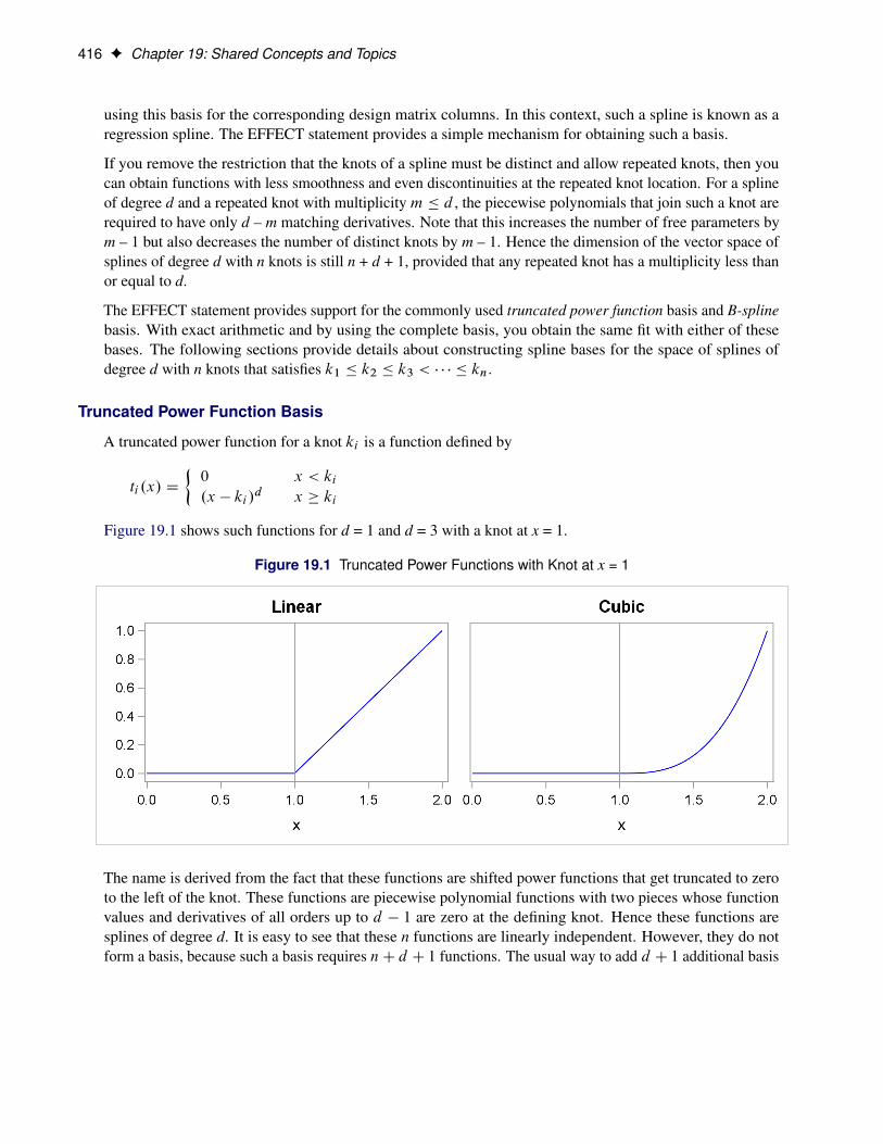
A truncated power function for a knot ki is a function defined by
ti .x/ D
�0 x < ki
.x � ki /d x � ki
Figure 19.1 shows such functions for d = 1 and d = 3 with a knot at x = 1.
Figure 19.1 Truncated Power Functions with Knot at x = 1
The name is derived from the fact that these functions are shifted power functions that get truncated to zeroto the left of the knot. These functions are piecewise polynomial functions with two pieces whose functionvalues and derivatives of all orders up to d � 1 are zero at the defining knot. Hence these functions aresplines of degree d. It is easy to see that these n functions are linearly independent. However, they do notform a basis, because such a basis requires nC d C 1 functions. The usual way to add d C 1 additional basis
Splines and Spline Bases F 417
functions is to use the polynomials 1; x; x2; : : : ; xd . These d C 1 functions together with the n truncatedpower functions ti .x/; i D 1; 2; : : : ; n form the truncated power basis.
Note that each time a knot is repeated, the associated exponent used in the corresponding basis functionis reduced by 1. For example, for splines of degree d with three repeated knots ki D kiC1 D kiC2 thecorresponding basis functions are ti .x/ D .x � ki /
dC
, tiC1.x/ D .x � ki /d�1C
, and tiC2.x/ D .x � ki /d�2C
.Provided that the multiplicity of each repeated knot is less than or equal to the degree, this constructioncontinues to yield a basis for the associated space of splines.
The main advantage of the truncated power function basis is the simplicity of its construction and the easeof interpreting the parameters in a model that corresponds to these basis functions. However, there aretwo weaknesses when you use this basis for regression. These functions grow rapidly without bound as xincreases, resulting in numerical precision problems when the x data span a wide range. Furthermore, manyor even all of these basis functions can be nonzero when evaluated at some x value, resulting in a designmatrix with few zeros that precludes the use of sparse matrix technology to speed up computation. Thisweakness can be addressed by using a B-spline basis.
B-Spline Basis
A B-spline basis can be built by starting with a set of Haar basis functions, which are functions that are 1between adjacent knots and 0 elsewhere, and then applying a simple linear recursion relationship d times,yielding the n C d C 1 needed basis functions. For the purpose of building the B-spline basis, the nprespecified knots are referred to as internal knots. This construction requires d additional knots, knownas boundary knots, to be positioned to the left of the internal knots, and MAX.d; 1/ boundary knots to bepositioned to the right of the internal knots. The actual values of these boundary knots can be arbitrary. TheEFFECT statement provides several methods for placing the needed boundary knots, including the commonmethod of using repeated values of the data extremes as the boundary knots. The boundary knot placementaffects the precise form of the basis functions that are generated, but it does not affect the following twodesirable properties:
1. The B-spline basis functions are nonzero over an interval that spans at most d C 2 knots. This yieldsdesign matrix columns each of whose rows contain at most d C 2 adjacent nonzero entries.
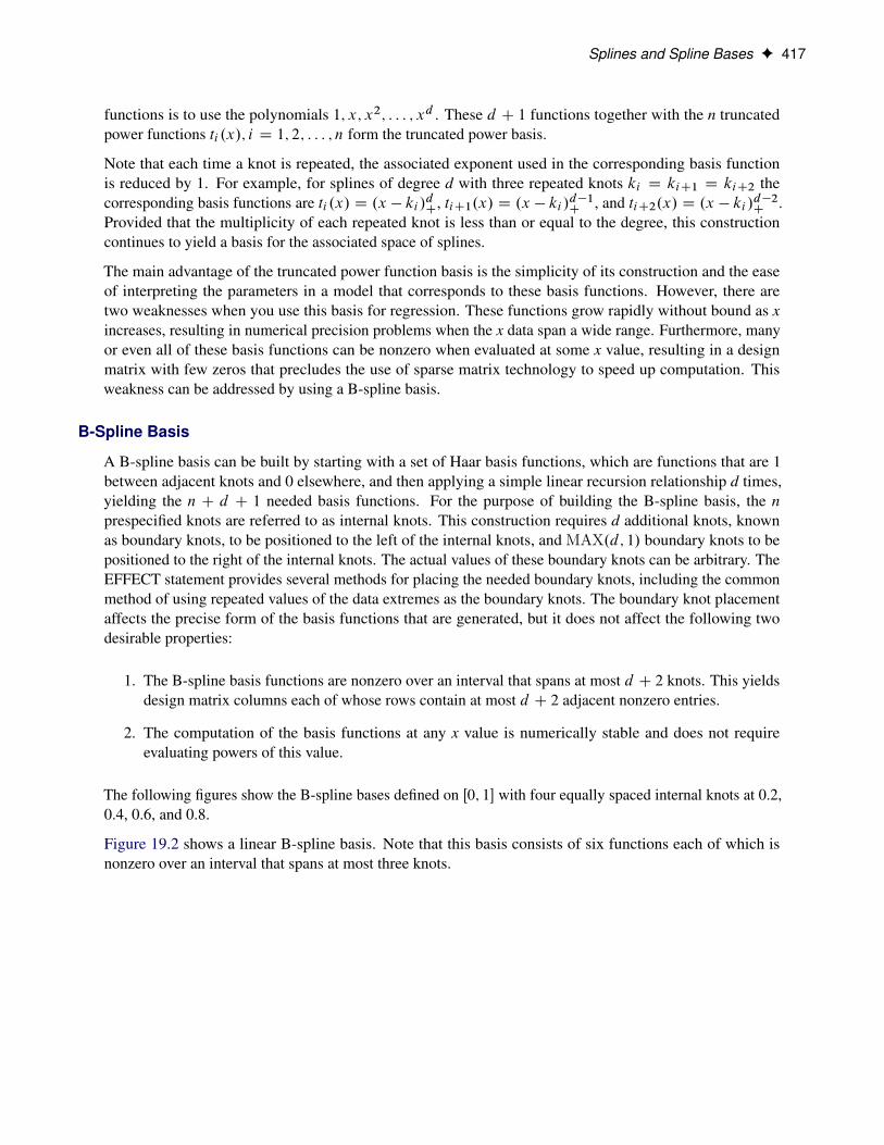
2. The computation of the basis functions at any x value is numerically stable and does not requireevaluating powers of this value.
The following figures show the B-spline bases defined on Œ0; 1� with four equally spaced internal knots at 0.2,0.4, 0.6, and 0.8.
Figure 19.2 shows a linear B-spline basis. Note that this basis consists of six functions each of which isnonzero over an interval that spans at most three knots.

418 F Chapter 19: Shared Concepts and Topics
Figure 19.2 Linear B-Spline Basis with Four Equally Spaced Interior Knots
Figure 19.3 shows a cubic B-spline basis where the needed boundary knots are positioned at x = 0 and x = 1.Note that this basis consists of eight functions, each of which is nonzero over an interval spanning at mostfive knots.
Figure 19.3 Cubic B-Spline Basis with Four Equally Spaced Interior Knots
Figure 19.4 shows a different cubic B-spline basis where the needed left-side boundary knots are positionedat –0.6, –0.4, –0.2, and 0. The right-side boundary knots are positioned at 1, 1.2, 1.4, and 1.6. Note that, asin the basis shown in Figure 19.3, this basis consists of eight functions, each of which is nonzero over aninterval spanning at most five knots. The different positioning of the boundary knots has merely changed theshape of the individual basis functions.

Splines and Spline Bases F 419
Figure 19.4 Cubic B-Spline Basis with Equally Spaced Boundary and Interior Knots
You can find details about this construction in Hastie, Tibshirani, and Friedman (2001).
Natural Cubic Spline Basis
Natural cubic splines are cubic splines with the additional restriction that the splines are required to be linearbeyond the extreme knots. Some authors prefer the terminology “restricted cubic splines” to “natural cubicsplines.” The space of unrestricted cubic splines on n knots has the dimension nC4. Imposing the restrictionsthat the cubic polynomials beyond the first and last knot reduce to linear polynomials reduces the number ofdegrees of freedom by 4, and so a basis for the natural cubic splines consists of n functions. Starting from thetruncated power function basis for the unrestricted cubic splines, you can obtain a reduced basis by imposinglinearity constraints. You can find details about this construction in Hastie, Tibshirani, and Friedman (2001).Figure 19.5 shows this natural cubic spline basis defined on Œ0; 1� with four equally spaced internal knotsat 0.2, 0.4, 0.6, and 0.8. Note that this basis consists of four basis functions that are all linear beyond theextreme knots at 0.2 and 0.8.
Figure 19.5 Natural Cubic Spline Basis with Four Equally Spaced Knots

420 F Chapter 19: Shared Concepts and Topics
EFFECTPLOT Statement
This statement applies to the following SAS/STAT procedures: GEE, GENMOD, LOGISTIC, ORTHOREG,and PLM. It also applies to the RELIABILITY procedure in SAS/QC software.
The EFFECTPLOT statement produces a display (effect plot) of a complex fitted model and provides optionsfor changing and enhancing the display. One simple effect plot is the display for a linear regression of theresponse Y on a single predictor X: the regression line is drawn with the predicted response on the Y axisand the covariate on the X axis. The regression line can be enhanced by displaying the observations andadding confidence and prediction limits. When your model is more complicated—with more continuous andcategorical covariates, nestings and interactions, and link functions—the effect plots display the behavior ofsome covariates over their ranges while holding other covariates at some fixed values; this can enable easierinterpretation and explanation of the resulting model.
By default, a single plot is produced based on the type of response variable and the number of continuousand classification covariates in the model. You can also specify options to do the following:
� select the variables to display in the plots
� produce multiple plots based on the following: the levels of classification covariates; the minimum,maximum, mean, or middle (midrange) value of continuous covariates; and specified values of thecovariates
� specify different fixed values for continuous and classification covariates that are not displayed in theplot
� panel and unpanel plots
� select variables to slice or group by
� display (or remove from display) observations and confidence limits
Syntax: EFFECTPLOT StatementEFFECTPLOT < plot-type < (plot-definition-options) > > < / options > ;
The available plot-types and their plot-definition-options are described in Table 19.13. Table 19.15 lists theoptions that can be specified after a slash (/) for any plot-type, and Table 19.16 lists additional options thatenhance specific plot-types. Full descriptions of the plot-definition-options and the other options are providedin the section “Dictionary of Options” on page 422.

Syntax: EFFECTPLOT Statement F 421
Table 19.13 Plot-Types and Plot-Definition-Options
Plot-Type and Description Plot-Definition-Options
BOXDisplays a box plot of continuous response data at eachlevel of a CLASS effect, with predicted valuessuperimposed and connected by a line. This is analternative to the INTERACTION plot-type.
PLOTBY= variable or CLASS effectX= CLASS variable or effect
CONTOURDisplays a contour plot of predicted values against twocontinuous covariates.
PLOTBY= variable or CLASS effectX= continuous variableY= continuous variable
FITDisplays a curve of predicted values versus acontinuous variable.
PLOTBY= variable or CLASS effectX= continuous variable
INTERACTIONDisplays a plot of predicted values (possibly with errorbars) versus the levels of a CLASS effect. Thepredicted values are connected with lines and can begrouped by the levels of another CLASS effect.
PLOTBY= variable or CLASS effectSLICEBY= variable or CLASS effectX= CLASS variable or effect
MOSAICDisplays a mosaic plot of predicted values using up tothree CLASS effects.
PLOTBY= variable or CLASS effectX= CLASS effects
SLICEFITDisplays a curve of predicted values versus acontinuous variable grouped by the levels of aCLASS effect.
PLOTBY= variable or CLASS effectSLICEBY= variable or CLASS effectX= continuous variable
By default, a single plot is produced based on the type of response variable and the number of continuousand classification covariates in the model, as shown in Table 19.14. If you have a polytomous responsemodel, then the response variable is treated as the grouping classification variable in this table. If your modeldoes not fit into Table 19.14, then a default plot is not produced; however, specifying the plot-type argumentdisplays a plot with the extra continuous covariates fixed at their mean values and the extra classificationcovariates fixed at their reference levels.
Table 19.14 Default Plot-Types
Number of Covariates Type of Response VariableClassification Continuous Continuous or Binary Polytomous
1 0 INTERACTION INTERACTION with groups2 0 INTERACTION with groups None0 1 FIT SLICEFIT0 2 CONTOUR None1 1 SLICEFIT None

422 F Chapter 19: Shared Concepts and Topics
Table 19.15 and Table 19.16 list the options that can be specified after a slash (/) to enhance the effect plots.
Table 19.15 Available Options for All Plot-Types
AT< args > ILINK NOOFFSET NROWS=ab PREDLABEL=ATLEN= INDIVIDUALa NCOLS=ab OBS< (options) > UNPACKATORDER= LINKb NOOBSab PLOTBYLEN=a Not available for the BOX plot-type.b Not available for the MOSAIC plot-type.
NOTE: If your model contains an offset variable and the NOOFFSET option is not specified or not valid, thenthe predicted values are computed only at the observations. In this case, the FIT and SLICEFIT plot-typesdisplay scatter plots of the predicted values, the CONTOUR plot-type displays the residuals against twocontinuous covariates but with no fitted surface, the INTERACTION plot-type does not connect the predictedvalues with lines, and the BOX plot-type is unchanged.
Table 19.16 Additional Options for Each Plot-Type
Plot-Type Options
BOX CLUSTER, CONNECT, NOCLUSTER, NOCONNECT,YRANGE=
CONTOUR EXTEND=, GRIDSIZE=
FIT ALPHA=, EXTEND=, GRIDSIZE=, NOCLI, NOCLM,NOLIMITS, SMOOTH, YRANGE=
INTERACTION ALPHA=, CLI, CLM, CLUSTER, CONNECT, LIMITS,NOCLUSTER, NOCONNECT, POLYBAR, YRANGE=
MOSAIC ADDCELL, BIN, EQUAL, NOBORDER, TYPE=
SLICEFIT ALPHA=, CLI, CLM, EXTEND=, GRIDSIZE=, LIMITS,YRANGE=
Dictionary of Options
You can specify the following EFFECTPLOT options.
ADDCELL<=value>adds value to the weight of every cell in the MOSAIC plot-type. You can specify value as anynonnegative number. If you do not specify a value, then value=0.5. This enables you to add somedimension to zero frequency cells.
ALPHA=valuespecifies the significance level, 0 � value � 1, for producing 100.1 � value=2/% prediction andconfidence limits. By default, value=0.05.

Syntax: EFFECTPLOT Statement F 423
AT < contopt > < classopt > < variable1< (CODED) >=varopt < variable2< (CODED) >=varopt . . . > >
where contopt= MEAN | MIN | MAX | MIDRANGE
classopt= ALL | REF
varopt= contopts | number-list | classopts | ’class-level’. . . ’class-level’specifies values at which to fix continuous and CLASS variables when they are not used in X=, Y=,SLICEBY=, or PLOTBY= effects. The contopt keyword fixes continuous variables at their mean,minimum, maximum, or midrangeD 1
2.minimumCmaximum/; the default is to use the mean. The
classopt keyword either fixes a CLASS variable at its reference (last) level or indicates that all levelsof the CLASS variable should be processed; the default is to use the reference level. The varopt valuesenable you to specify contopt and classopt keywords or to specify lists of numbers or class levels.You can specify a CLASS variable only once in the AT specification, but you can specify a continuousvariable multiple times; for example, the following syntax is valid when X is a continuous variable:
effectplot / at(x=min max x=0 to 2 by 1 x=2 5 7);
Duplicate AT values are suppressed, so the last X=2 value is ignored.
You can also specify coded plug-in values for CLASS variable levels when computing the predictedvalues x0ˇ. For example, suppose a CLASS variable A with two levels={0,1} is in the model. Theninstead of using the coding for A in the x vector by specifying AT(A=all), AT(A=ref) or AT(A=’0’’1’), you can specify a numeric list to plug in. For example, if the proportion of A’s that equal 0in the data set is 0.3, then you can input the proportions for all levels of the variable by specifyingAT(A(CODED)=0.3 0.7). Under GLM coding, A=0 is coded as “1 0” and A=1 is coded as “0 1”, sothe plug-in specification replaces both of these codings with “0.3 0.7”. Under REFERENCE coding,A=0 is coded as “1” and A=1 is coded as “0”, so this specification replaces both of these codings with“0.3” followed by “0.7”; however, if another variable is nested within A, then only “0.3” is used. Toplug in values, you must specify a multiple of the number of parameters used for the CLASS variableor, if a variable is nested within the CLASS variable, a multiple of the number of levels of the CLASSvariable.
The coded plug-in values are distributed through the rest of the model effects in the following fashion.If a variable is nested within a plug-in variable, then its coding is multiplied by the plug-in value forthe level it is nested in. If a variable interacts with a plug-in variable, its coding is multiplied by theappropriate plug-in value for the level it is interacting with. Lag, multimember, polynomial, and splineconstructed effects are affected only by interactions and nestings. If the plug-in variable is part of acollection effect, then its values are replaced by the plug-in values; collection effects are also affectedby interactions and nestings.
The AT levels are used for computing the predicted values. If the OBS option is also specified, then allobservations are still displayed in all the plots. For example, if you specify the options AT(A=’1’)OBS, then the fitted values are computed by using A=1, but all the observations are displayed with theirpredicted values computed at their observed level of A. If you want to display only a subset of theobservations based on the levels of a CLASS variable, then you must specify either the PLOTBY=option or the OBS(BYAT) option.
ATLEN=nspecifies the maximum length (1 � n � 256) of the levels of the AT variables that are displayed infootnotes and headers. By default, up to 256 characters of the CLASS levels are displayed, and thecontinuous AT levels are displayed with a BEST format that has a width greater than or equal to 5,

424 F Chapter 19: Shared Concepts and Topics
which distinguishes each level. CAUTION: If the levels of your AT variables are not unique when thefirst n characters are displayed, then the levels are combined in the plots but not in the underlyingcomputations. Also, at most n characters for continuous AT variables are displayed.
ATORDER=ASCENDING | DESCENDINGuses the AT values for continuous variables in ascending or descending order as specified. By default,values are used in the order of their first appearance in the AT option.
BINdisplays the statistic for the MOSAIC plot-type with a discrete coloring scheme.
CLIdisplays normal (Wald) prediction limits. This option is available only for normal distributions withidentity links. If your model is from a Bayesian analysis, then sampling-based intervals are computed;for more information, see the section “Analysis Based on Posterior Estimates” on page 7266 inChapter 89, “The PLM Procedure.”
CLMdisplays confidence limits. These are computed as the normal (Wald) confidence limits for the linearpredictor, and if the ILINK option is specified, the limits are also back-transformed by the inverse linkfunction. If your model is from a Bayesian analysis, then sampling-based intervals are computed; formore information, see the section “Analysis Based on Posterior Estimates” on page 7266 in Chapter 89,“The PLM Procedure.”
CLUSTER< =percent >modifies the BOX and INTERACTION plot-types by displaying the levels of the SLICEBY= effectside by side. You can specify percent as a percentage of half the distance between X levels. Thepercent value must be between 0.1 and 1; the default percent depends on the number of X levels, thenumber of SLICEBY levels, and the number of PLOTBY levels for INTERACTION plot-types. Youcan remove default clustering by specifying the NOCLUSTER option.
CONNECTmodifies the BOX and INTERACTION plot-types by connecting the predicted values with a line. Youcan remove default connecting lines by specifying the NOCONNECT option.
EQUALcauses every cell in the MOSAIC plot-type to have the same dimensions.
EXTEND=DATA | valueextends continuous covariate axes by value � 1
2range in both directions, where range is the range
of the X axis. Specifying the DATA keyword displays curves to the range of the data within theappropriate SLICEBY=, PLOTBY=, and AT level. For the CONTOUR plot-type, value=0.05 bydefault; other plot-types set the default value to 0. When constructed effects are present, only theEXTEND=DATA option is available.
GRIDSIZE=nspecifies the resolution of curves by computing the predicted values at n equally spaced values on theX axis and specifies the resolution of surfaces by computing the predicted values on an n�n grid ofpoints. Default values are n = 200 for curves and bands, n = 50 for surfaces, and n = 2 for lines. Ifresults of a Bayesian or bootstrap analysis are being displayed, then the defaults are n = 500000/B,where B is the number of samples, the upper limit is equal to the usual defaults, and the lower limit isequal to 20.

Syntax: EFFECTPLOT Statement F 425
ILINKdisplays the fit on the scale of the inverse link function. In particular, the results are displayed on theprobability scale for logistic regression. By default, a procedure displays the fit on either the link orinverse link scale.
INDIVIDUALdisplays individual probabilities for polytomous response models with cumulative links on the scaleof the inverse link function. This option is not available when the LINK option is specified, andconfidence limits are not available when you specify this option.
LIMITSinvokes the CLI and CLM options.
LINKdisplays the fit on the scale of the link function—that is, the linear predictor. Probabilities or observedproportions near 0 and 1 are transformed to˙20. By default, a procedure displays the fit on either thelink or inverse link scale.
NCOLS=nspecifies the maximum number of columns in a paneled plot. This option is not available with theBOX plot-type.
The default choice of NROWS= and NCOLS= is based on the number of PLOTBY= and AT levels. Ifonly one plot is displayed in a panel, then NROWS=1 and NCOLS=1 and the plots are produced as ifyou specified only the UNPACK option. If only two plots are displayed in a panel, then NROWS=1and NCOLS=2. For all other cases, a 2�2, 2�3, or 3�3 panel is chosen based on how much of the lastpanel is used, with ties going to the larger panels. For example, if 14 plots are being created, then thisrequires either four 2�2 panels with 50% of the last panel filled, three 2�3 panels with 33% of thelast panel filled, or two 3�3 panels with 55% of the last panel filled; in this case, the 3�3 panels arechosen.
If you specify both the NROWS= and NCOLS= options, then those are the values used. However, ifyou specify only one of the options but have fewer plots, then the panel size is reduced; for example,if you specify NROWS=6 but have only four plots, then a plot that has four rows and one column isproduced.
NOBORDERremoves the border from the cells in the MOSAIC plot-type. Otherwise, the color of the cells that werenot observed in the data set is hidden by the border.
NOCLIsuppresses the prediction limits.
NOCLMsuppresses the confidence limits.
NOCLUSTERmodifies the BOX and INTERACTION plot-types by preventing the side-by-side display of the levelsof the SLICEBY= effect.

426 F Chapter 19: Shared Concepts and Topics
NOCONNECTmodifies the BOX and INTERACTION plot-types by suppressing the line that connects the predictedvalues.
NOLIMITSinvokes the NOCLI and NOCLM options.
NOOBSsuppresses the display of observations and overrides the specification of the OBS= option.
NOOFFSETMOFF
moves the offset for a Poisson regression model to the response side of the equation. If the ILINKoption is also specified, then the rate is displayed on the Y axis; if the LINK option is also specified,then the log of the rate is displayed on the Y axis. Without the NOOFFSET option, the predictedvalues are computed and displayed only for the observations.
NROWS=nspecifies the maximum number of rows in a paneled plot. This option is not available with the BOXplot-type. For more information, see the NCOLS= option.
OBS< (obs-options) >displays observations in the effect plots. An input data set is required; hence the OBS option is notavailable with PROC PLM. The OBS option is overridden by the NOOBS option. When the ILINKoption is specified with binary response variables, then either the observed proportions or a coded valueof the response is displayed. For polytomous response variables, the observed values are overlaid ontothe fitted curves unless the LOCATION= option is specified. Whether or not observations are displayedby default depends on the procedure. If the PLOTBY= option is specified, then the observations thatare displayed in each plot are from the corresponding PLOTBY= level for classification effects; forcontinuous effects, all observations are displayed in every plot.
You can specify the following obs-options:
BYATsubsets the observations by AT level and by the PLOTBY= level. If you specify the PLOTBY=option without specifying this option, the observations are displayed in the plots that correspondto their PLOTBY= level without regard to any classification variables specified in the AT option.However, for FIT plot-types a distance can be computed and displayed (for more information,see the DISTANCE option). This option is ignored when there are no AT variables.
CDISPLAY=NONE | OUTLINE | GRADIENT | OUTLINEGRADIENTcontrols the display of observations in contour plots. The keyword OUTLINE displays theobservations as circles, GRADIENT displays gradient-colored dots, OUTLINEGRADIENTdisplays gradient-filled-circles, and NONE suppresses the display of the observations. Thedefault is CDISPLAY=OUTLINEGRADIENT.
CGRADIENT=RESIDUAL | DEPENDENTspecifies what the gradient shading of the observed values in the CONTOUR plot-type represents.The RESIDUAL keyword shades the observations by the raw residual value and displays thefitted surface as a line contour plot. The DEPENDENT keyword shades the observations by theresponse variable value and displays the fitted surface as a contour shaded on the same scale. Thedefault is CGRADIENT=DEPENDENT.

Syntax: EFFECTPLOT Statement F 427
DEPTH=depthspecifies the number of overlapping observations that can be distinguished by adjusting theirtransparency; you can specify 1 � depth � 100. By default, DEPTH=1. The DEPTH= option isavailable with the FIT, SLICEFIT, and INTERACTION plot-types.
DISTANCEdisplays observations in FIT plot-types with a color gradient that indicates how far the observationis from the AT and PLOTBY= level. This option is ignored unless an AT or PLOTBY= option isspecified.
The distance is computed as the square root of the following number: for each continuous ATand PLOTBY= variable, add the square of the difference from the observed value divided bythe range of the variable; for each CLASS AT and PLOTBY= variable, add 1 if the CLASSlevels are different. Thus the largest possible distance is the square root of the number of AT andPLOTBY= variables. Observations at zero distance are displayed by using the darkest color, andthe color fades as the distance increases.
The unpacked panels compute the maximum distance within each panel and hence do not use thesame gradient across all panels. Also, the PANELS panel-type computes the maximum distancewithin each PLOTBY= level, so a different gradient is used for each PLOTBY= level. All otherpanel-types compute the maximum distance across all observations and therefore use the samegradient in every plot.
FITATCLASScomputes fitted values only for class levels that are observed in the data set. This option is ignoredwhen the GLM parameterization is used.
FRINGEdisplays observations in a fringe (rug) plot at the bottom of the plot. This option is available onlywith the FIT and SLICEFIT plot-types.
JITTER< (jitter-options) >shifts (jitters) the observations. By default, the jittering in the X direction is achieved by adding arandom number that is generated according to a normal distribution with mean=0 and standarddeviation=x-jitter=2 and truncating at˙x-jitter , where x-jitter=0.01 times the range of the X axis;the jittering in the Y direction is performed independently but in the same fashion. The JITTERoption is not available with the BOX plot-type. You can specify the following jitter-options:
FACTOR=factor sets the jitter to factor times the range of the axis, and jitters in both the X andY directions. You can specify 0 � factor � 1.
SEED=seed specifies an integer to use as the initial seed for the random number generator. Ifyou do not specify a seed, or if you specify a value less than or equal to zero, then thetime of day from the computer clock is used to generate an initial seed.
X=x-jitter sets the jitter to x-jitter for the X direction; the jitter in the Y direction is assumedto be 0 unless the Y= option is also specified. You can specify x-jitter � 0. The X=option is not available for the INTERACTION plot-type. This option is ignored if theFACTOR= option is also specified.
Y=y-jitter sets the jitter to y-jitter for the Y direction; the jitter in the X direction is assumed tobe 0 unless the X= option is also specified. You can specify y-jitter � 0. This option isignored if the FACTOR= option is also specified.
428 F Chapter 19: Shared Concepts and Topics
LABEL< =OBS >labels markers with their observation number.
LOCATION=locationspecifies where the observed values for polytomous response models are displayed when theSLICEBY= variable is the response. This option is available only with the SLICEFIT andINTERACTION plot-types. The observations are always displayed at their appropriate X-axisvalue, but their Y-axis location can depend on the specification of the YRANGE= option or onthe minimum and maximum computed predicted values in addition to the specified location. Youcan specify the following locations:
BOTTOM< =factor > displays the first response level at the minimum predicted value, anddisplays succeeding response levels above the first level at factor �range intervals,where range is the range of the predicted values. You can specify 0 � factor � 1, butthe largest usable value, which corresponds to LOCATION=SPREAD, is factor= 1
k,
where kC1 is the number of response levels that are displayed. By default, factor=0.03.
CURVE displays the observations for polytomous response models at their predicted values.For displays on the LINK scale, the reference level is displayed at the maximum value.This method is the default.
FIRST displays the observations for a response level at the first displayed predicted value forthat response level.
MAX displays the observations for a response level at the maximum displayed predictedvalue for that response level.
MIDDLE displays the observations for a response level at the middle of the displayed predictedvalues for that response level.
MIN displays the observations for a response level at the minimum displayed predictedvalue for that response level.
SPREAD displays the observations with the response levels evenly spread across the Y axis.
TOP< =factor > displays the last response level at the maximum predicted value, and displayspreceding response levels below the last level at factor �range intervals, where rangeis the range of the predicted values. You can specify 0 � factor � 1, but the largestusable value, which corresponds to LOCATION=SPREAD, is factor= 1
k, where k+1 is
the number of response levels that are displayed. By default, factor=0.03.
PLOTBY< (panel-type) >=effect< =numeric-list >specifies a variable or CLASS effect at whose levels the predicted values are computed and the plotsare displayed. You can specify the response variable as the effect for polytomous response models.The panel-type argument specifies the method in which the plots are grouped for the display. You canspecify the following panel-types:
COLUMNSspecifies that the columns within each panel correspond to different levels of the PLOTBY=effect and hence the rows correspond to different AT levels.

Syntax: EFFECTPLOT Statement F 429
PACKspecifies that plots be displayed in the panels as they are produced, with no control over theplacement of the PLOTBY= and AT levels.
PANELS | LEVELSspecifies that each level of the PLOTBY= effect begin a new panel of plots and the AT levelsdefine the plots within the panels.
ROWSspecifies that the rows within each panel correspond to different levels of the PLOTBY= effectand hence the columns correspond to different AT levels.
This option is ignored with the BOX plot-type; box plots are always displayed in an unpacked fashion,grouped by the PLOTBY= and AT levels. If you specify a continuous variable as the effect , then eitheryou can specify a numeric-list of values at which to display that variable or, by default, five equallyspaced values from the minimum variable value to its maximum are displayed.
The default panel-type is based on the number of PLOTBY= and AT levels, as shown in the followingtable.
Number ofPLOTBY= Levels
Number ofAT Levels
Resultingpanel-type
1 1 (UNPACK)>1 1 PACK
1 >1 PACK2 >1 ROWS3 >1 COLUMNS
>3 >1 PANELS
The default dimensions of the panels are also based on the number of PLOTBY= and AT levels; formore information, see the NCOLS= option.
Specification of the panel-type is honored except in the following cases. If you specify a panel-typebut produce only one plot, specify the NROWS=1 and NCOLS=1 options, or specify the UNPACKoption, then the plots are produced as if you specified only the UNPACK option. If you specify thePANELS panel-type with only one AT level, then the plots are produced with the UNPACK option.However, if you specify the PANELS panel-type but the PLOTBY= effect has only one level, then thepanel-type is changed to PACK.
PLOTBYLEN=nspecifies the maximum length (1 � n � 256) of the levels of the PLOTBY= variables, which aredisplayed in footnotes and headers. By default, up to 256 characters of the CLASS levels are displayed.CAUTION: If the levels of your PLOTBY= variables are not unique when the first n characters aredisplayed, then the levels are combined in the plots but not in the underlying computations.
POLYBARdisplays polytomous response data as a stacked histogram whose bar heights are defined by theindividual predicted value. Your response variable must be the effect that is specified in the SLICEBY=option. If you specify the INDIVIDUAL option, then the histogram bars are displayed side by side. Ifyou specify the CLM option, then error bars are displayed on the side-by-side histogram bars.

430 F Chapter 19: Shared Concepts and Topics
PREDLABEL='label 'specifies a label to be displayed on the Y axis. The default Y-axis label is determined by your model.For the CONTOUR plot-type, this option changes the title to “label for Y.”
SHOWCLEGENDdisplays the gradient legend for the CONTOUR plot-type. This option has no effect when theOBS(CGRADIENT=RESIDUAL) option is also specified.
SLICEBY=NONE | effect< =numeric-list >displays the fitted values at the different levels of the specified variable or CLASS effect. You canspecify the response variable as the effect for polytomous response models. Use this option to modifythe SLICEFIT, INTERACTION, and BOX plot-types. If you specify a continuous variable as theeffect , then either you can specify a numeric-list of values at which to display that variable or, bydefault, five equally spaced values from the minimum variable value to its maximum are displayed.The NONE keyword is available for preventing the INTERACTION plot-type from slicing by a secondclassification covariate. The SLICEBY=NONE option is not available for the SLICEFIT plot-type,because that is the same as the FIT plot-type. The BOX plot-type accepts only classification effects.
SMOOTHoverlays a loess smooth on the FIT plot-type for models that have only one continuous predictor. Thisoption is not available for binary or polytomous response models.
TYPE=PREDICTED | PARQUET | GOFspecifies the type of display for the MOSAIC plot-types. For effects that are specified as in the X=option, the TYPE=PREDICTED and TYPE=GOF mosaic plots create cells by dividing the X axisproportional to the total weight in each level of the x-effect , then dividing the Y axis according to theweight in each level of the y-effect within the x-effect levels, and dividing the X2 axis according to theweight in each level of the x2-effect within the x-effect and y-effect levels. The TYPE=PARQUETplot uses the predicted probabilities instead of the weights to determine the dimensions of the cells.
The default TYPE=PREDICTED mosaic plot colors the cells according to their predicted values(probabilities for binary and polytomous response models) computed at the AT and PLOTBY levels.The TYPE=GOF plot displays the Pearson goodness-of-fit statistic as in Friendly (2000), with theexpected value computed at the AT and PLOTBY levels. For a cell iy defined by the axis levels,the PLOTBY and AT levels, and the response level y, let Wiy
be the sum of all the weights of theobservations in that cell, let Wi D
Py Wiy
be the sum of the weights across all response levels, andlet OYy be the predicted response for that cell, where y is the event level for binary response models, andOYy D Pr.Y D yjiy/ for binary and multinomial models. Then the Pearson goodness-of-fit statistic is
computed as
Wiy�Wi
OYqWiOY
The TYPE=GOF plot is not available when you have continuous covariates in the model. TheTYPE=PARQUET plot shades the cells with their observed weights and is available only with binaryor polytomous response data.

ODS Graphics: EFFECTPLOT Statement F 431
UNPACKsuppresses paneling. By default, multiple plots can appear in some output panels. Specify UNPACKto display each plot separately.
X=effect | (x-effect < y-effect < x2-effect > >)specifies values to display on the X axis. For the BOX and INTERACTION plot-types, effect can be aCLASS effect in the MODEL statement. For the FIT, SLICEFIT, and CONTOUR plot-types, effectcan be any continuous variable in the model. For the MOSAIC plot-types, you can specify CLASSeffects (or the response variable if you have a multinomial model) as the effect or x-effect to displayon the X axis, as the y-effect to display on the Y axis, and as the x2-effect to display on the X2 (upper)axis.
Y=argsspecifies values to display on the Y axis for the CONTOUR plot-type. The Y= argument can be anycontinuous variable in the model.
YRANGE=CLIP | (< min >< ,max >)displays the predicted values on the Y axis in the range [min,max]. The YRANGE=CLIP optionhas the same effect as specifying the minimum predicted value as min and the maximum predictedvalue as max . The axis might extend beyond your specified values. By default, when the Y axisdisplays predicted probabilities, the entire Y axis, [0,1], is displayed. This option is useful if yourpredicted probabilities are all contained in some subset of this range. This option is not available withthe CONTOUR plot-type.
ODS Graphics: EFFECTPLOT StatementTo produce the EFFECTPLOT displays, ODS Graphics must be enabled. For more information about ODSGraphics, see Chapter 21, “Statistical Graphics Using ODS.” The available graph names are provided inTable 19.17.
Table 19.17 Graphs Produced by the EFFECTPLOT Statement
ODS Graph Name Plot Description
BoxFitPlot A box plot of the responses at each level of one classification effect, overlaidwith a plot of the predicted values
ContourFitPlot A contour plot of the fitted surface against two continuous covariatesContourFitPanel A panel of ContourFitPlotsFitPlot A curve of the predicted values plotted against one continuous covariateFitPanel A panel of FitPlotsInteractionPlot A plot of the predicted values (connected by a line) against one classification
effect, possibly for each level of a second classification effectInteractionPanel A panel of InteractionPlotsMosaicFitPlot A mosaic plot of the predicted values categorized by one to three classifica-
tion effectsSliceFitPlot A curve of the predicted values against one continuous covariate for each
level of a second classification covariateSliceFitPanel A panel of SliceFitPlots

432 F Chapter 19: Shared Concepts and Topics
Examples: EFFECTPLOT Statement
Example 19.1: A Saddle SurfaceMyers (1976) analyzes an experiment reported by Frankel (1961) that is aimed at maximizing the yield ofmercaptobenzothiazole (MBT) by varying processing time and temperature. Myers uses a two-factor modelin which the estimated surface does not have a unique optimum. The objective is to find the settings of timeand temperature in the processing of the chemical that maximize the yield. The following statements createthe data set d:
data d;input Time Temp MBT @@;label Time = "Reaction Time (Hours)"
Temp = "Temperature (Degrees Centigrade)"MBT = "Percent Yield Mercaptobenzothiazole";
datalines;4.0 250 83.8 20.0 250 81.7 12.0 250 82.4
12.0 250 82.9 12.0 220 84.7 12.0 280 57.912.0 250 81.2 6.3 229 81.3 6.3 271 83.117.7 229 85.3 17.7 271 72.7 4.0 250 82.0;
In the following statements, the ORTHOREG procedure fits a response surface regression model to thedata and uses the EFFECTPLOT statement to create a slice of the response surface. The FIT plot-typerequests plots of the predicted yield against the Time variable, and the PLOTBY= option specifies that theTemp variable is fixed at five equally spaced values so that five fitted regression curves are displayed inOutput 19.1.1.
ods graphics on;proc orthoreg data=d;
model MBT=Time|Time|Temp|Temp@2;effectplot fit(x=time plotby=temp);
run;ods graphics off;
The displays in Output 19.1.1 show that the slope of the surface changes as the temperature increases.

Example 19.1: A Saddle Surface F 433
Output 19.1.1 Panel of Fit Plots
It might be more informative to see these results in one graphic, so the following statements specify theSLICEFIT plot-type to overlay plots of the predicted yield versus time, fixed at several values of temperature.In this case, the SLICEBY= option is specified to explicitly use the same four temperatures as used in theexperiment.
ods graphics on;proc orthoreg data=d;
model MBT=Time|Time|Temp|Temp@2;effectplot slicefit(x=time sliceby=temp=229 250 271 280);
run;ods graphics off;

434 F Chapter 19: Shared Concepts and Topics
Output 19.1.2 shows that to optimize the yield you should choose either low temperatures and long times orhigh temperatures and short times.
Output 19.1.2 Fit Plot Grouped (Sliced) by Temp
Another plot might explain the reason for these conflicting results more clearly. The following statementsproduce the default EFFECTPLOT statement display, enhanced by the OBS(JITTER) option to jitter theobservations so that you can see the replicated points:
ods graphics on;proc orthoreg data=d;
model MBT=Time|Time|Temp|Temp@2;effectplot / obs(jitter(seed=39393));
run;ods graphics off;

Example 19.1: A Saddle Surface F 435
Output 19.1.3 shows that the reason for the changing slopes is that the surface is at a saddle point. Thissurface does not have an optimum point.
Output 19.1.3 Contour Fit Plot with Jittered Observations

436 F Chapter 19: Shared Concepts and Topics
Example 19.2: Unbalanced Two-Way ANOVAThis example uses data from Kutner (1974, p. 98) to illustrate a two-way analysis of variance. The originaldata source is Afifi and Azen (1972, p. 166). The following statements create the data set a:
data a;input drug disease @;do i=1 to 6;
input y @;output;
end;datalines;
1 1 42 44 36 13 19 221 2 33 . 26 . 33 211 3 31 -3 . 25 25 242 1 28 . 23 34 42 132 2 . 34 33 31 . 362 3 3 26 28 32 4 163 1 . . 1 29 . 193 2 . 11 9 7 1 -63 3 21 1 . 9 3 .4 1 24 . 9 22 -2 154 2 27 12 12 -5 16 154 3 22 7 25 5 12 .;
In the following statements, PROC GENMOD fits two classification variables and their interaction to Y. Thefirst EFFECTPLOT statement displays the default graphic, which plots the predicted values against Diseasefor each of the three Drug levels. The OBS option also displays the observations in the plot. The secondEFFECTPLOT statement modifies the default to plot the predicted values against Drug for each of the threeDisease levels. The CLM option is specified to produce 95% confidence bars for the means.
ods graphics on;proc genmod data=a;
class drug disease;model y=disease drug disease*drug / d=n;effectplot / obs;effectplot interaction(sliceby=disease) / clm;
run;ods graphics off;
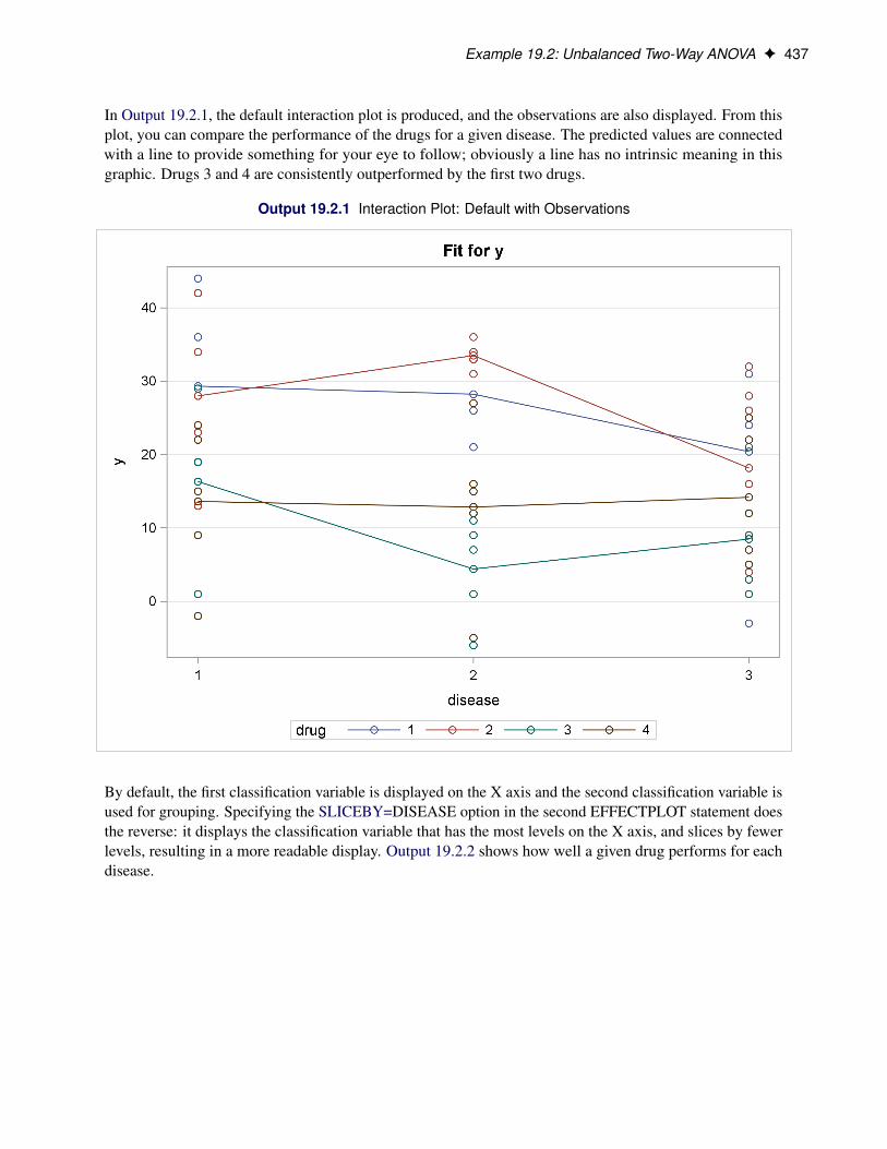
Example 19.2: Unbalanced Two-Way ANOVA F 437
In Output 19.2.1, the default interaction plot is produced, and the observations are also displayed. From thisplot, you can compare the performance of the drugs for a given disease. The predicted values are connectedwith a line to provide something for your eye to follow; obviously a line has no intrinsic meaning in thisgraphic. Drugs 3 and 4 are consistently outperformed by the first two drugs.
Output 19.2.1 Interaction Plot: Default with Observations
By default, the first classification variable is displayed on the X axis and the second classification variable isused for grouping. Specifying the SLICEBY=DISEASE option in the second EFFECTPLOT statement doesthe reverse: it displays the classification variable that has the most levels on the X axis, and slices by fewerlevels, resulting in a more readable display. Output 19.2.2 shows how well a given drug performs for eachdisease.

438 F Chapter 19: Shared Concepts and Topics
Output 19.2.2 Interaction Plot with Specified SLICEBY= Effect
In the following statements, the BOX plot-type is requested to display box plots of the predictions by eachcombination of drug and disease. The second EFFECTPLOT statement displays the same information byusing an INTERACTION plot-type and specifies the OBS option to display the individual observations.The third EFFECTPLOT statement displays the predictions in a MOSAIC plot. The fourth EFFECTPLOTstatement creates an interaction plot of predictions versus drug for each of the Disease levels and displaysthem in a panel.
ods graphics on;proc genmod data=a;
class drug disease;model y=drug disease drug*disease / d=n;effectplot box;effectplot interaction(x=drug*disease) / obs;effectplot mosaic;effectplot interaction(plotby=disease);
run;ods graphics off;

Example 19.2: Unbalanced Two-Way ANOVA F 439
In the box plot in Output 19.2.3, the predicted values are displayed as circles; they coincide with the mean ofthe data at each level, all of which are displayed as diamonds. The predicted values are again connected bylines. It is difficult to draw any conclusions from this graphic.
Output 19.2.3 Box Fit Plot

440 F Chapter 19: Shared Concepts and Topics
Output 19.2.4 shows the interaction plot at every combination of Drug and Disease. This plot is identical tothe box plot in Output 19.2.3, except the boxes are replaced by the actual observations. Again, it is difficultto see any pattern in the plot.
Output 19.2.4 Interaction Plot with Specified X= Effect

Example 19.2: Unbalanced Two-Way ANOVA F 441
Output 19.2.5 displays the mosaic plot. You can see that drugs 1 and 2 consistently outperform the other twodrugs.
Output 19.2.5 Mosaic Plot

442 F Chapter 19: Shared Concepts and Topics
Output 19.2.6 groups the observations by Disease, and for each disease displays the effectiveness of the fourdrugs in a panel of plots.
Output 19.2.6 Interaction Plot with Specified PLOTBY= Effect

Example 19.3: Logistic Regression F 443
Example 19.3: Logistic RegressionConsider a study of the analgesic effects of treatments on elderly patients with neuralgia. Two test treatmentsand a placebo are compared. The response variable is whether the patient reported pain or not. Researchersrecorded the age and gender of 60 patients and the duration of complaint before the treatment began. Thefollowing DATA step creates the data set Neuralgia:
data Neuralgia;input Treatment $ Sex $ Age Duration Pain $ @@;datalines;
P F 68 1 No B M 74 16 No P F 67 30 NoP M 66 26 Yes B F 67 28 No B F 77 16 NoA F 71 12 No B F 72 50 No B F 76 9 YesA M 71 17 Yes A F 63 27 No A F 69 18 YesB F 66 12 No A M 62 42 No P F 64 1 YesA F 64 17 No P M 74 4 No A F 72 25 NoP M 70 1 Yes B M 66 19 No B M 59 29 NoA F 64 30 No A M 70 28 No A M 69 1 NoB F 78 1 No P M 83 1 Yes B F 69 42 NoB M 75 30 Yes P M 77 29 Yes P F 79 20 YesA M 70 12 No A F 69 12 No B F 65 14 NoB M 70 1 No B M 67 23 No A M 76 25 YesP M 78 12 Yes B M 77 1 Yes B F 69 24 NoP M 66 4 Yes P F 65 29 No P M 60 26 YesA M 78 15 Yes B M 75 21 Yes A F 67 11 NoP F 72 27 No P F 70 13 Yes A M 75 6 YesB F 65 7 No P F 68 27 Yes P M 68 11 YesP M 67 17 Yes B M 70 22 No A M 65 15 NoP F 67 1 Yes A M 67 10 No P F 72 11 YesA F 74 1 No B M 80 21 Yes A F 69 3 No;
The Neuralgia data set contains five variables. The Pain variable is the response. A specification of Pain=Yesindicates that the patient felt pain, and Pain=No indicates that the patient did not feel pain. The variableTreatment is a categorical variable with three levels: A and B represent the two test treatments, and Prepresents the placebo treatment. The gender of the patients is given by the categorical variable Sex. Thevariable Age is the age of the patients, in years, when treatment began. The duration of complaint, in months,before the treatment began is given by the variable Duration.
In the following statements, a complex model that includes classification and continuous covariates and aninteraction term is fit to the Neuralgia data. When you try to create a default effect plot from this model,computations stop because the best type of plot cannot easily be determined.
ods graphics on;proc logistic data=Neuralgia;
class Treatment Sex / param=ref;model Pain= Treatment|Sex Age Duration;effectplot;
run;ods graphics off;
To produce an effect plot for this model, you need to first choose the type of plot to be created. In this case,since there are both classification and continuous covariates on the model, a SLICEFIT plot-type displays the

444 F Chapter 19: Shared Concepts and Topics
first continuous covariate (Age) on the X axis and displays fit curves that correspond to each level of the firstclassification covariate (Treatment). The following statements produce Output 19.3.1.
ods graphics on;proc logistic data=Neuralgia;
class Treatment Sex / param=ref;model Pain= Treatment|Sex Age Duration;effectplot slicefit;
run;ods graphics off;
By default, effect plots from PROC LOGISTIC are displayed on the probability scale. The predicted valuesare computed at the mean of the Duration variable, 16.73, and at the reference level of the Sex variable, M.Observations are also displayed on the sliced-fit plot in Output 19.3.1. While the display of binary responsescan give you a feel for the spread of the data, it does not enable you to evaluate the fit of the model.
Output 19.3.1 Default Fit Plot Sliced by Treatment
In the following statements, an INTERACTION plot-type is specified for the Treatment variable, with the Sexeffect chosen for grouping the fits. The Age and Duration variables are set to their mean values for computingthe predicted values. The NOOBS option suppresses the display of the binary observations on this plot. TheLINK option is specified to display the fit on the LOGIT scale; if there is no interaction between Treatmentand Sex, then the resulting curves shown in Output 19.3.2 will have similar slopes across the treatments.

Example 19.3: Logistic Regression F 445
ods graphics on;proc logistic data=Neuralgia;
class Treatment Sex / param=ref;model Pain= Treatment|Sex Age Duration;effectplot interaction(x=Treatment sliceby=Sex) / noobs link;
run;ods graphics off;
In Output 19.3.2, the slopes of the lines seem “parallel” across the treatments, corroborating the nonsignifi-cance of the interaction terms.
Output 19.3.2 Interaction Plot of an Interaction Effect
In the following statements, the interaction effect is removed, and the Duration variable is investigatedfurther. The PLOTBY(ROWS)= option displays the Sex levels in the rows of a panel of plots, and the AToption computes the fits for several values of the Duration main effect in the columns of the panel. TheOBS(FRINGE) option moves the observations to a fringe (rug) plot at the bottom of the plot, the observationsare subsetted and displayed according to the value of the PLOTBY= variable, and the JITTER option makesoverlaid fringes more visible. A STORE statement is also specified to save the model information for a laterdisplay. These statements produce Output 19.3.3.
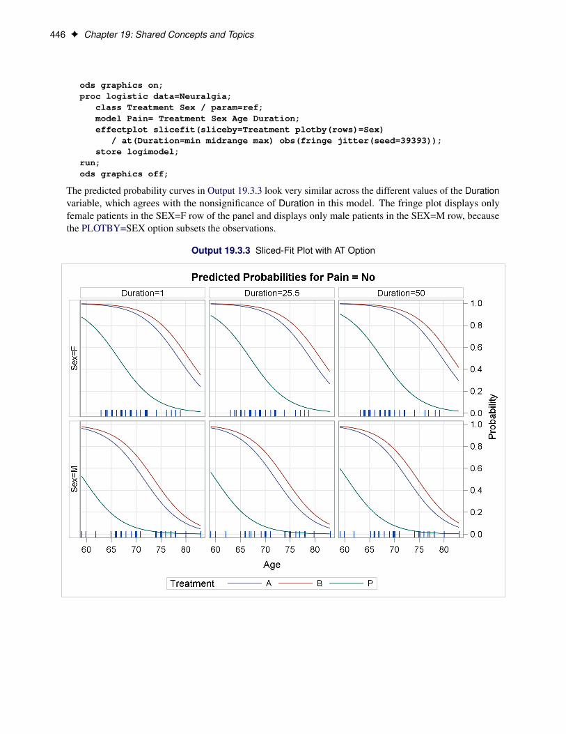
446 F Chapter 19: Shared Concepts and Topics
ods graphics on;proc logistic data=Neuralgia;
class Treatment Sex / param=ref;model Pain= Treatment Sex Age Duration;effectplot slicefit(sliceby=Treatment plotby(rows)=Sex)
/ at(Duration=min midrange max) obs(fringe jitter(seed=39393));store logimodel;
run;ods graphics off;
The predicted probability curves in Output 19.3.3 look very similar across the different values of the Durationvariable, which agrees with the nonsignificance of Duration in this model. The fringe plot displays onlyfemale patients in the SEX=F row of the panel and displays only male patients in the SEX=M row, becausethe PLOTBY=SEX option subsets the observations.
Output 19.3.3 Sliced-Fit Plot with AT Option

Example 19.3: Logistic Regression F 447
The following statements use the stored model and the PLM procedure to display a panel of contour plots:
ods graphics on;proc plm restore=logimodel;
effectplot contour(plotby=Treatment) / at(Sex=all);run;ods graphics off;
Output 19.3.4 again confirms that Duration is not significant.
Output 19.3.4 Contour Fit Panel
448 F Chapter 19: Shared Concepts and Topics
ESTIMATE Statement
This statement documentation applies to the following SAS/STAT procedures:GEE, LIFEREG, LOGISTIC, ORTHOREG, PHREG, PLM, PROBIT, QUANTREG, SURVEYLOGISTIC,SURVEYPHREG, and SURVEYREG. It also applies to the RELIABILITY procedure in SAS/QC software.The ESTIMATE statement in the GENMOD, GLIMMIX, GLM, and MIXED procedures are documented inthe respective procedure chapters.
The ESTIMATE statement provides a mechanism for obtaining custom hypothesis tests. Estimates areformed as linear estimable functions of the form Lˇ. You can perform hypothesis tests for the estimablefunctions, construct confidence limits, and obtain specific nonlinear transformations.
Syntax: ESTIMATE StatementESTIMATE < 'label ' > estimate-specification < (DIVISOR=n) >
< , < 'label ' > estimate-specification < (DIVISOR=n) > > < , . . . >< / options > ;
The basic element of the ESTIMATE statement is the estimate-specification, which consists of model effectsand their coefficients. An estimate-specification takes the general form
effect name < effect values . . . >
The following elements can appear in the ESTIMATE statement:
'label ' is an optional label that identifies the particular row of the estimate in the output.
effect identifies an effect that appears in the MODEL statement. The keyword INTERCEPT canbe used as an effect when an intercept is fitted in the model. You do not need to includeall effects that are in the MODEL statement.
values are constants that are elements of the L matrix and are associated with the fixed andrandom effects. There are two basic methods of specifying the entries of the L matrix.The traditional representation—also known as the positional syntax—relies on enteringcoefficients in the position they assume in the L matrix. For example, in the followingstatements the elements of L that are associated with the b main effect receive a 1 in thefirst position and a –1 in the second position:
class a b;model y = a b a*b;estimate 'B at A2' b 1 -1 a*b 0 0 1 -1;

Syntax: ESTIMATE Statement F 449
The elements that are associated with the interaction receive a 1 in the third position and a–1 in the fourth position. In order to specify coefficients correctly for the interaction term,you need to know how the levels of a and b vary in the interaction, which is governed bythe order of the variables in the CLASS statement. The nonpositional syntax is designedto make it easier to enter coefficients for interactions and is necessary to enter coefficientsfor effects that are constructed with the EFFECT statement. In square brackets you enterthe coefficient followed by the associated levels of the CLASS variables. If B has twolevels and A has three levels, the previous ESTIMATE statement, by using nonpositionalsyntax for the interaction term, becomes the following statement:
estimate 'B at A2' b 1 -1 a*b [1, 2 1] [-1, 2 2];
The previous statement assigns value 1 to the interaction where A is at level 2 and B is atlevel 1, and it assigns –1 to the interaction where both classification variables are at level 2.The comma that separates the entry for the L matrix from the level indicators is optional.Further details about the nonpositional contrast syntax and its use with constructed effectscan be found in the section “Positional and Nonpositional Syntax for Coefficients inLinear Functions” on page 459.
Based on the estimate-specifications in your ESTIMATE statement, the procedure constructs the matrix L totest the hypothesis H WLˇ D 0. The procedure supports nonpositional syntax for the coefficients of modeleffects in the ESTIMATE statement. For details see the section “Positional and Nonpositional Syntax forCoefficients in Linear Functions” on page 459.
The procedure then produces for each row l of L an approximate t test of the hypothesis H W lˇ D 0. You canalso obtain multiplicity-adjusted p-values and confidence limits for multirow estimates with the ADJUST=option.
Note that multirow estimates are permitted. Unlike releases prior to SAS 9.22, you do not need to specify a'label ' for every row of the estimate; the procedure constructs a default label if a label is not specified.
If the procedure finds the estimate to be nonestimable, then it displays “Non-est” for the estimate entry.
Table 19.18 summarizes important options in the ESTIMATE statement. All ESTIMATE options aresubsequently discussed in alphabetical order.
Table 19.18 ESTIMATE Statement Options
Option Description
Construction and Computation of Estimable FunctionsDIVISOR= Specifies a list of values to divide the coefficientsNOFILL Suppresses the automatic fill-in of coefficients for higher-order
effectsSINGULAR= Tunes the estimability checking difference
Degrees of Freedom and p-valuesADJUST= Determines the method for multiple comparison adjustment of
estimatesALPHA=˛ Determines the confidence level (1 � ˛)
450 F Chapter 19: Shared Concepts and Topics
Table 19.18 continued
Option Description
LOWER Performs one-sided, lower-tailed inferenceSTEPDOWN Adjusts multiplicity-corrected p-values further in a step-down
fashionTESTVALUE= Specifies values under the null hypothesis for testsUPPER Performs one-sided, upper-tailed inference
Statistical OutputCL Constructs confidence limitsCORR Displays the correlation matrix of estimatesCOV Displays the covariance matrix of estimatesE Prints the L matrixJOINT Produces a joint F or chi-square test for the estimable functionsPLOTS= Requests ODS statistical graphics if the analysis is sampling-basedSEED= Specifies the seed for computations that depend on random
numbers
Generalized Linear ModelingCATEGORY= Specifies how to construct estimable functions with multinomial
dataEXP Exponentiates and displays estimatesILINK Computes and displays estimates and standard errors on the inverse
linked scale
You can specify the following options in the ESTIMATE statement after a slash (/).
ADJDFE=SOURCE
ADJDFE=ROWspecifies how denominator degrees of freedom are determined when p-values and confidence limitsare adjusted for multiple comparisons with the ADJUST= option. When you do not specify theADJDFE= option, or when you specify ADJDFE=SOURCE, the denominator degrees of freedom formultiplicity-adjusted results are the denominator degrees of freedom for the final effect that is listed inthe ESTIMATE statement from the “Type III” table.
The ADJDFE=ROW setting is useful if you want multiplicity adjustments to take into account thatdenominator degrees of freedom are not constant across estimates. For example, this can be the casewhen the denominator degrees of freedom are computed by the Satterthwaite method or according toKenward and Roger (1997).
The ADJDFE= option has an effect only in mixed models that use these degree-of-freedom methods.It is not supported by the procedures that perform chi-square-based inference (LOGISTIC, PHREG,and SURVEYLOGISTIC).

Syntax: ESTIMATE Statement F 451
ADJUST=BON
ADJUST=SCHEFFE
ADJUST=SIDAK
ADJUST=SIMULATE< (sim-options) >
ADJUST=Trequests a multiple comparison adjustment for the p-values and confidence limits for the estimates. Theadjusted quantities are produced in addition to the unadjusted quantities. Adjusted confidence limits areproduced if the CL or ALPHA= option is in effect. For a description of the adjustments, see Chapter 48,“The GLM Procedure,” and Chapter 81, “The MULTTEST Procedure,” and the documentation for theADJUST= option in the LSMEANS statement.
If the STEPDOWN option is in effect, the p-values are further adjusted in a step-down fashion.
ALPHA=numberrequests that a t type confidence interval be constructed with confidence level 1 – number . The valueof number must be between 0 and 1; the default is 0.05. If the “Estimates” table shows infinite degreesof freedom, then the confidence interval is a z type interval.
CATEGORY=category-optionsspecifies how to construct estimates and multiplicity corrections for models with multinomial data(ordinal or nominal). This option is also important for constructing sets of estimable functions for F orchi-square tests with the JOINT option.
The category-options are used to indicate how response variable levels are treated in constructing theestimable functions. Possible values for the category-options are the following:
JOINTcomputes the estimable functions for every nonredundant category and treats them as a set. Forexample, a three-row ESTIMATE statement in a model with three response categories leads tosix estimable functions.
SEPARATEcomputes the estimable functions for every nonredundant category in turn. For example, athree-row ESTIMATE statement in a model with three response categories leads to two sets ofthree estimable functions.
quoted-value-listcomputes the estimable functions only for the specified list of values. The list must consist offormatted values of the response categories, and you must specify an estimate-specification foreach response category in the list.
Consider the following ESTIMATE statements in the LOGISTIC procedure for an ordinal model withresponse categories ‘vg’, ‘g’, ‘m’, ‘b’, and ‘vb’. Because there are five response categories, there arefour nonredundant categories for the cumulative link model.

452 F Chapter 19: Shared Concepts and Topics
proc logistic data=icecream;class brand / param=glm;model taste(order=data) = brand / link=logit;freq count;
estimate brand 1 -1,intercept 1 brand 0 1 / category='m','vg';
estimate intercept 1 brand 1 / category=jointadjust=simulate(seed=1);
estimate brand 1 -1,brand 1 1 -2 / category=separate
adjust=bon;run;
The first ESTIMATE statement requests a two-row estimable function. The result is produced fortwo of the four nonredundant response categories. The second ESTIMATE statement produces four ttests, one for each nonredundant category. The multiplicity adjustment with p-value computation bysimulation treats the four estimable functions as a unit for family-wise Type I error protection. Thethird ESTIMATE statement computes a two-row estimable function and reports its results separatelyfor all nonredundant categories. The Bonferroni adjustment in this statement applies to a family of twotests that correspond to the two-row estimable function. Four Bonferroni adjustments for sets of sizetwo are performed.
The CATEGORY= option is supported only by the procedures that support generalized linear modeling(GEE, LOGISTIC, and SURVEYLOGISTIC) and by PROC PLM when it is used to perform statisticalanalyses on item stores created by these procedures.
CHISQrequests that chi-square tests be performed in addition to F tests, when you request an F test with theJOINT option. This option has no effect in procedures that produce chi-square statistics by default.
CLrequests that t type confidence limits be constructed. If the procedure shows the degrees of freedom inthe “Estimates” table as infinite, then the confidence limits are z intervals. The confidence level is 0.95by default, and you can change the confidence level with the ALPHA= option. The confidence intervalsare adjusted for multiplicity when you specify the ADJUST= option. However, if a step-down p-valueadjustment is requested with the STEPDOWN option, only the p-values are adjusted for multiplicity.
CORRdisplays the estimated correlation matrix of the linear combination of the parameter estimates.
COVdisplays the estimated covariance matrix of the linear combination of the parameter estimates.
DF=numberspecifies the degrees of freedom for the t test and confidence limits. This option is not supported by theprocedures that perform chi-square-based inference (LOGISTIC, PHREG, and SUVEYLOGISTIC).

Syntax: ESTIMATE Statement F 453
DIVISOR=value-listspecifies a list of values by which to divide the coefficients so that fractional coefficients can be enteredas integer numerators. If you do not specify value-list , a default value of 1.0 is assumed. Missingvalues in the value-list are converted to 1.0.
If the number of elements in value-list exceeds the number of rows of the estimate, the extra values areignored. If the number of elements in value-list is less than the number of rows of the estimate, the lastvalue in value-list is copied forward.
If you specify a row-specific divisor as part of the specification of the estimate row, this value multipliesthe corresponding divisor that is implied by the value-list . For example, the following statement dividesthe coefficients in the first row by 8, and the coefficients in the third and fourth row by 3:
estimate 'One vs. two' A 2 -2 (divisor=2),'One vs. three' A 1 0 -1 ,'One vs. four' A 3 0 0 -3 ,'One vs. five' A 1 0 0 0 -1 / divisor=4,.,3;
Coefficients in the second row are not altered.
Erequests that the L matrix coefficients be displayed.
EXPrequests exponentiation of the estimate. When you model data with the logit, cumulative logit, orgeneralized logit link functions, and the estimate represents a log odds ratio or log cumulative oddsratio, the EXP option produces an odds ratio. In proportional hazards model, this option producesestimates of hazard ratios. If you specify the CL or ALPHA= option, the (adjusted) confidence boundsare also exponentiated.
The EXP option is supported only by PROC PHREG, PROC SURVEYPHREG, the procedures thatsupport generalized linear modeling (GEE, LOGISTIC and SURVEYLOGISTIC), and by PROC PLMwhen it is used to perform statistical analyses on item stores created by these procedures.
ILINKrequests that the estimate and its standard error also be reported on the scale of the mean (the inverselinked scale). The computation of the inverse linked estimate depends on the estimation mode. Forexample, if the analysis is based on a posterior sample when a BAYES statement is present, theinversely linked estimate is the average of the inversely linked values across the sample of posteriorparameter estimates. If the analysis is not based on a sample of parameter estimates, the procedurecomputes the value on the mean scale by applying the inverse link to the estimate. The interpretationof this quantity depends on the effect values specified in your ESTIMATE statement and on the linkfunction. For example, in a model for binary data with logit link the following statements compute
1
1C expf�.˛1 � ˛2/g
where ˛1 and ˛2 are the fixed-effects solutions that are associated with the first two levels of theclassification effect A:

454 F Chapter 19: Shared Concepts and Topics
class A;model y = A / dist=binary link=logit;estimate 'A one vs. two' A 1 -1 / ilink;
This quantity is not the difference of the probabilities that are associated with the two levels,
�1 � �2 D1
1C expf�ˇ0 � ˛1g�
1
1C expf�ˇ0 � ˛2g
The standard error of the inversely linked estimate is based on the delta method. If you also specifythe CL option, the procedure computes confidence limits for the estimate on the mean scale. Inmultinomial models for nominal data, the limits are obtained by the delta method. In other models theyare obtained from the inverse link transformation of the confidence limits for the estimate. The ILINKoption is specific to an ESTIMATE statement.
The ILINK option is supported only by the procedures that support generalized linear modeling(GEE, LOGISTIC and SURVEYLOGISTIC) and by PROC PLM when it is used to perform statisticalanalyses on item stores created by these procedures.
JOINT< (joint-test-options) >requests that a joint F or chi-square test be produced for the rows of the estimate. The JOINT option inthe ESTIMATE statement essentially replaces the CONTRAST statement.
When the LOWERTAILED or the UPPERTAILED options are in effect, or if the BOUNDS optiondescribed below is in effect, the JOINT option produces the chi-bar-square statistic according toSilvapulle and Sen (2004). This statistic uses a simulation-based approach to compute p-valuesin situations where the alternative hypotheses of the estimable functions are not simple two-sidedhypotheses. See the section “Joint Hypothesis Tests with Complex Alternatives, the Chi-Bar-SquareStatistic” on page 461 for more information about this test statistic.
You can specify the following joint-test-options in parentheses:
ACC= specifies the accuracy radius for determining the necessary sample size in the simulation-basedapproach of Silvapulle and Sen (2004) for tests with order restrictions. The value of must bestrictly between 0 and 1; the default value is 0.005.
EPS=�specifies the accuracy confidence level for determining the necessary sample size in the simulation-based approach of Silvapulle and Sen (2004) for tests with order restrictions. The value of � mustbe strictly between 0 and 1; the default value is 0.01.
LABEL='label 'assigns an identifying label to the joint test. If you do not specify a label, the first non-defaultlabel for the ESTIMATE rows is used to label the joint test.
NOEST
ONLYperforms only the F or chi-square test and suppresses other results from the ESTIMATE statement.This option is useful for emulating the CONTRAST statement that is available in other procedures.
Syntax: ESTIMATE Statement F 455
NSAMP=nspecifies the number of samples for the simulation-based method of Silvapulle and Sen (2004).If n is not specified, it is constructed from the values of the ALPHA=˛, the ACC= , and theEPS=� options. With the default values for , �, and ˛ (0.005, 0.01, and 0.05, respectively),NSAMP=12,604 by default.
CHISQadds a chi-square test if the procedure produces an F test by default.
BOUNDS=value-listspecifies boundary values for the estimable linear function. The null value of the hypothesisis always zero. If you specify a positive boundary value z, the hypotheses are H W � D 0,HaW W � > 0 with the added constraint that � < z. The same is true for negative boundary values.The alternative hypothesis is then HaW � < 0 subject to the constraint � > �jzj. If you specify amissing value, the hypothesis is assumed to be two-sided. The BOUNDS option enables you tospecify sets of one- and two-sided joint hypotheses. If all values in value-list are set to missing,the procedure performs a simulation-based p-value calculation for a two-sided test.
LOWER
LOWERTAILEDrequests that the p-value for the t test be based only on values that are less than the test statistic. Atwo-tailed test is the default. A lower-tailed confidence limit is also produced if you specify the CL orALPHA= option.
Note that for ADJUST=SCHEFFE the one-sided adjusted confidence intervals and one-sided adjustedp-values are the same as the corresponding two-sided statistics, because this adjustment is based ononly the right tail of the F distribution.
If you request a joint test with the JOINT option, then a one-sided left-tailed order restriction is appliedto all estimable functions, and the corresponding chi-bar-square statistic of Silvapulle and Sen (2004)is computed in addition to the two-sided, standard, F or chi-square statistic. See the JOINT option forhow to control the computation of the simulation-based chi-bar-square statistic.
NOFILLsuppresses the automatic fill-in of coefficients of higher-order effects.
PLOTS=plot-optionsproduces ODS statistical graphics of the distribution of estimable functions if the procedure performsthe analysis in a sampling-based mode. For example, this is the case when procedures support a BAYESstatement and perform a Bayesian analysis. The estimable functions are then computed for each of theposterior parameter estimates, and the “Estimates” table reports simple descriptive statistics for theevaluated functions. The PLOTS= option enables you in this situation to visualize the distribution ofthe estimable function. The following plot-options are available:
ALLproduces all possible plots with their default settings.
BOXPLOT< (boxplot-options) >produces box plots of the distribution of the estimable function across the posterior sample. Aseparate box is generated for each estimable function, and all boxes appear on a single graph bydefault. You can affect the appearance of the box plot graph with the following options:

456 F Chapter 19: Shared Concepts and Topics
ORIENTATION=VERTICAL | HORIZONTAL
ORIENT=VERT | HORIZspecifies the orientation of the boxes. The default is vertical orientation of the box plots.
NPANELPOS=numberspecifies how to break the series of box plots across multiple panels. If the NPANELPOSoption is not specified, or if number equals zero, then all box plots are displayed in a singlegraph; this is the default. If a negative number is specified, then exactly up to jnumber j ofbox plots are displayed per panel. If number is positive, then the number of boxes per panelis balanced to achieve small variation in the number of box plots per graph.
DISTPLOT< (distplot-options) >
DIST< (distplot-options) >generates panels of histograms with a kernel density overlaid. A separate plot in each panelcontains the results for each estimable function. You can specify the following distplot-options inparentheses:
BOX | NOBOXcontrols the display of a horizontal box plot of the estimable function’s distribution acrossthe posterior sample below the graph. The BOX option is enabled by default.
HIST | NOHISTcontrols the display of the histogram of the estimable function’s distribution across theposterior sample. The HIST option is enabled by default.
NORMAL | NONORMALcontrols the display of a normal density estimate on the graph. The NONORMAL option isenabled by default.
KERNEL | NOKERNELcontrols the display of a kernel density estimate on the graph. The KERNEL option isenabled by default.
NROWS=numberspecifies the highest number of rows in a panel. The default is 3.
NCOLS=numberspecifies the highest number of columns in a panel. The default is 3.
UNPACKunpacks the panel into separate graphics.
NONEdoes not produce any plots.
SEED=numberspecifies the seed for the sampling-based components of the computations for the ESTIMATE statement(for example, chi-bar-square statistics and simulated p-values). The value of number must be an integer.The seed is used to start the pseudo-random number generator for the simulation. If you do not specifya seed, or if you specify a value less than or equal to zero, the seed is generated from reading the

Syntax: ESTIMATE Statement F 457
time of day from the computer clock. There could be multiple ESTIMATE statements with SEED=specifications and there could be other statements that can supply a random number seed. Since theprocedure has only one random number stream, the initial seed is shown in the SAS log.
SINGULAR=numbertunes the estimability checking. If v is a vector, define ABS(v) to be the largest absolute value of theelements of v. If ABS(L � LT) is greater than c*number for any row of L in the contrast, then Lˇis declared nonestimable. Here, T is the Hermite form matrix .X0X/�X0X, and c is ABS(L), exceptwhen it equals 0, and then c is 1. The value for number must be between 0 and 1; the default is 1E–4.
STEPDOWN< (step-down-options) >requests that multiplicity adjustments for the p-values of estimates be further adjusted in a step-downfashion. Step-down methods increase the power of multiple testing procedures by taking advantageof the fact that a p-value is never declared significant unless all smaller p-values are also declaredsignificant. The STEPDOWN adjustment combined with ADJUST=BON corresponds to the methodsof Holm (1979) and “Method 2” of Shaffer (1986); this is the default. Using step-down-adjustedp-values combined with ADJUST=SIMULATE corresponds to the method of Westfall (1997).
If the ESTIMATE statement is applied with a STEPDOWN option in a mixed model where the degrees-of-freedom method is that of Kenward and Roger (1997) or of Satterthwaite, then step-down-adjustedp-values are produced only if the ADJDFE=ROW option is in effect.
Also, the STEPDOWN option affects only p-values, not confidence limits. For ADJUST=SIMULATE,the generalized least squares hybrid approach of Westfall (1997) is used to increase Monte Carloaccuracy. You can specify the following step-down-options in parentheses after the STEPDOWNoption:
MAXTIME=nspecifies the time (in seconds) to be spent computing the maximal logically consistent sequentialsubsets of equality hypotheses for TYPE=LOGICAL. The default is MAXTIME=60. If theMAXTIME value is exceeded, the adjusted tests are not computed. When this occurs, you cantry increasing the MAXTIME value. However, note that there are common multiple comparisonsproblems for which this computation requires a huge amount of time—for example, all pairwisecomparisons between more than 10 groups. In such cases, try to use TYPE=FREE (the default)or TYPE=LOGICAL(n) for small n.
ORDER=PVALUE
ORDER=ROWSspecifies the order in which the step-down tests to be performed. ORDER=PVALUE is thedefault, with estimates being declared significant only if all estimates with smaller (unadjusted)p-values are significant. If you specify ORDER=ROWS, then significances are evaluated in theorder in which they are specified in the syntax.
REPORTspecifies that a report on the step-down adjustment be displayed, including a listing of thesequential subsets (Westfall 1997) and, for ADJUST=SIMULATE, the step-down simulationresults.

458 F Chapter 19: Shared Concepts and Topics
TYPE=LOGICAL< (n) >
TYPE=FREEspecifies how step-down adjustment are made. If you specify TYPE=LOGICAL, the step-downadjustments are computed by using maximal logically consistent sequential subsets of equalityhypotheses (Shaffer 1986; Westfall 1997). Alternatively, for TYPE=FREE, sequential subsetsare computed ignoring logical constraints. The TYPE=FREE results are more conservative thanthose for TYPE=LOGICAL, but they can be much more efficient to produce for many estimates.For example, it is not feasible to take logical constraints between all pairwise comparisons ofmore than about 10 groups. For this reason, TYPE=FREE is the default.
However, you can reduce the computational complexity of taking logical constraints into accountby limiting the depth of the search tree used to compute them, specifying the optional depthparameter as a number n in parentheses after TYPE=LOGICAL. As with TYPE=FREE, resultsfor TYPE=LOGICAL(n) are conservative relative to the true TYPE=LOGICAL results. But evenfor TYPE=LOGICAL(0) they can be appreciably less conservative than TYPE=FREE, and theyare computationally feasible for much larger numbers of estimates. If you do not specify n or if n= –1, the full search tree is used.
TESTVALUE=value-list
TESTMEAN=value-listspecifies the value under the null hypothesis for testing the estimable functions in the ESTIMATEstatement. The rules for specifying the value-list are very similar to those for specifying the divisorlist in the DIVISOR= option. If no TESTVALUE= is specified, all tests are performed as H WLˇ D 0.Missing values in the value-list also are translated to zeros. If you specify fewer values than rows inthe ESTIMATE statement, the last value in value-list is carried forward.
The TESTVALUE= option affects only p-values from individual, joint, and multiplicity-adjusted tests.It does not affect confidence intervals.
The TESTVALUE option is not available for the multinomial distribution, and the values are ignoredwhen you perform a sampling-based (Bayesian) analysis.
UPPER
UPPERTAILEDrequests that the p-value for the t test be based only on values that are greater than the test statistic. Atwo-tailed test is the default. An upper-tailed confidence limit is also produced if you specify the CL orALPHA= option.
Note that for ADJUST=SCHEFFE the one-sided adjusted confidence intervals and one-sided adjustedp-values are the same as the corresponding two-sided statistics, because this adjustment is based ononly the right tail of the F distribution.
If you request a joint test with the JOINT option, then a one-sided right-tailed order restriction is appliedto all estimable functions, and the corresponding chi-bar-square statistic of Silvapulle and Sen (2004)is computed in addition to the two-sided, standard, F or chi-square statistic. See the JOINT option forhow to control the computation of the simulation-based chi-bar-square statistic.

Positional and Nonpositional Syntax for Coefficients in Linear Functions F 459
Positional and Nonpositional Syntax for Coefficients in Linear FunctionsWhen you define custom linear hypotheses with the ESTIMATE statement, the procedure sets up an L vectoror matrix that conforms to the model effect solutions. (Note that the following remarks also apply to theLSMESTIMATE statement, where you specify coefficients of the matrix K which is then converted into acoefficient matrix that conforms to the model effects solutions.)
There are two methods for specifying the entries in a coefficient matrix (hereafter simply referred to as theL matrix); they are called the positional and nonpositional methods. In the positional form, which is thetraditional method, you provide a list of values that occupy the elements of the L matrix that is associatedwith the effect in question in the order in which the values are listed. For traditional model effects that consistof continuous and classification variables, the positional syntax is simpler in some cases (main effects) andmore cumbersome in others (interactions). When you work with effects that are constructed through theEFFECT statement, the nonpositional syntax is essential.
For example, consider the following two-way model with interactions where factors A and B have three andtwo levels, respectively:
proc logistic;class a b;model y = a b a*b;
run;
To test the difference of the B levels at the second level of A with an ESTIMATE statement (a slice), you needto assign coefficients 1 and –1 to the levels of B and to the levels of the interaction where A is at the secondlevel. Two examples of equivalent ESTIMATE statements that use positional and nonpositional syntax are asfollows:
estimate 'B at A2' b 1 -1 a*b 0 0 1 -1 ;estimate 'B at A2' b 1 -1 a*b [1 2 1] [-1 2 2];
Because A precedes B in the CLASS statement, the levels of the interaction are formed as˛1ˇ1; ˛1ˇ2; ˛2ˇ1; ˛2ˇ2; : : : . If B precedes A in the CLASS statement, you need to modify the coef-ficients accordingly:
proc logistic;class b a;model y = a b a*b;estimate 'B at A2' b 1 -1 a*b 0 1 0 0 -1 ;estimate 'B at A2' b 1 -1 a*b [1 1 2] [-1 2 2];estimate 'B at A2' b 1 -1 a*b [1, 1 2] [-1, 2 2];
run;
You can optionally separate the L value entry from the level indicators with a comma, as in the last ESTIMATEstatement.
The general syntax for defining coefficients with the nonpositional syntax is as follows:
effect-name [multiplier < , > level-values] . . . < [multiplier < , > level-values] >
The first entry in square brackets is the multiplier that is applied to the elements of L for the effect after thelevel-values have been resolved and any necessary action that forms L has been taken.

460 F Chapter 19: Shared Concepts and Topics
The level-values are organized in a specific form:
� The number of entries should equal the number of terms that are needed to construct the effect. Foreffects that do not contain any constructed effects, this number is simply the number of terms in thename of the effect.
� Values of continuous variables that are needed for the construction of the L matrix precede the levelindicators of CLASS variables.
� If the effect involves constructed effects, then you need to provide as many continuous and classificationvariables as are needed for the effect formation. For example, if a collection effect is defined as
class c;effect v = collection(x1 x2 c);
then a proper nonpositional syntax would be
v [0.5, 0.2 0.3 3]
� If an effect contains both regular terms (old-style effects) and constructed effects, then the order of thecoefficients is as follows: continuous values for old-style effects, class levels for classification variablesin old-style effects, continuous values for constructed effects, and finally class levels that are neededfor constructed effects. Assume that C has four levels so that effect v contributes six elements to the Lmatrix. When the procedure resolves this syntax, the values 0.2 and 0.3 are assigned to the positionsfor x1 and x2 and a 1 is associated with the third level of C. The resulting vector is then multiplied by0.5 to produce
Œ0:1 0:15 0 0 0:5 0�
Note that you enter the levels of the classification variables in the square brackets, not their formatted values.The ordering of the levels of classification variables can be gleaned from the “Class Level Information” table.
To specify values for continuous variables, simply give their value as one of the terms in the effect. Thenonpositional syntax in the following ESTIMATE statement is read as “1 times the value 0.4 in the columnthat is associated with level 2 of A”
proc phreg;class a / param=glm;model y = a a*x / s;lsmeans a / e at x=0.4;estimate 'A2 at x=0.4' intercept 1 a 0 1 a*x [1,0.4 2] / e;
run;
Because the value before the comma serves as a multiplier, the same estimable function could also beconstructed with the following statements:
estimate 'A2 at x=0.4' intercept 1 a 0 1 a*x [ 4, 0.1 2];estimate 'A2 at x=0.4' intercept 1 a 0 1 a*x [ 2, 0.2 2];estimate 'A2 at x=0.4' intercept 1 a 0 1 a*x [-1, -0.4 2];
Joint Hypothesis Tests with Complex Alternatives, the Chi-Bar-Square Statistic F 461
Note that continuous variables that are needed to construct an effect are always listed before any CLASSvariables.
When you work with constructed effects, the nonpositional syntax works in the same way. For example, thefollowing model contains a classification effect and a B-spline. The first two ESTIMATE statements producepredicted values for level 1 of C when the continuous variable x takes on the values 20 and 10, respectively.
proc orthoreg;class c;effect spl = spline(x / knotmethod=equal(5));model y = c spl;estimate 'C = 1 @ x=20' intercept 1 c 1 spl [1,20],
'C = 1 @ x=10' intercept 1 c 1 spl [1,10];estimate 'Difference' spl [1,20] [-1,10];
run;
In this example, the ORTHOREG procedure computes the spline coefficients for the first ESTIMATEstatement based on x = 20, and similarly in the second statement for x = 10. The third ESTIMATE statementcomputes the difference of the predicted values. Because the spline effect does not interact with theclassification variable, this difference does not depend on the level of C. If such an interaction is present,you can estimate the difference in predicted values for a given level of C by using the nonpositional syntax.Because the effect C*spl contains both old-style terms (C) and a constructed effect, you specify the valuesfor the old-style terms before assigning values to constructed effects.
proc orthoreg;class c;effect spl = spline(x / knotmethod=equal(5));model y = spl*c;estimate 'C2 = 1, x=20' intercept 1 c*spl [1,1 20];estimate 'C2 = 2, x=20' intercept 1 c*spl [1,2 20];estimate 'C diff at x=20' c*spl [1,1 20] [-1,2 20];
run;
It is recommended that you add the E option to the ESTIMATE or LSMESTIMATE statement to verify thatthe L matrix is formed according to your expectations.
In any row of an ESTIMATE statement you can choose positional and nonpositional syntax separately foreach effect. However, you cannot mix the two forms of syntax for coefficients of a single effect. For example,the following statement is not proper because both forms of syntax are used for the interaction effect:
estimate 'A1B1 - A1B2' b 1 -1 a*b 0 1 [-1, 1 2];
Joint Hypothesis Tests with Complex Alternatives, the Chi-Bar-SquareStatistic
Silvapulle and Sen (2004) propose a test statistic for testing hypotheses where the null or the alternativehypothesis or both involve inequalities. You can test special cases of these hypotheses with the JOINToption in the ESTIMATE and the LSMESTIMATE statement. Consider the k estimable functions Lˇ andthe hypotheses H0WLˇ D 0 and HaWLˇ � 0. The alternative hypothesis defines a convex cone C at theorigin. Suppose that under the null hypothesis Lb follows a multivariate normal distribution with mean 0and variance V. The restricted alternative prevents you from using the usual F or chi-square test machinery,

462 F Chapter 19: Shared Concepts and Topics
since the distribution of the test statistic under the alternative might not follow the usual rules. Silvapulle andSen (2004) coined a statistic that takes into account the projection of the observed estimate onto the convexcone formed by the alternative parameter space. This test statistic is called the chi-bar-square statistic, andp-values are obtained by simulation; see, in particular, Chapter 3.4 in Silvapulle and Sen (2004).
Briefly, let U be a multivariate normal random variable with mean 0 and variance matrix V. The chi-bar-squarestatistic is the random variable
�2D U0V�1U �Q
Q D min�2C
.U � �/0V�1.U � �/
and it can be motivated by a geometric argument. The quadratic form in Q is the V-projection of U ontothe cone C. Suppose that this projected point is QU. If U 2 C, then Q = 0 and QU D U. If U is completelyoutside of the cone C, then QU is a point on the surface of the cone. Similarly, U0V�1U is the length of thesegment from the origin to U in the V-space with norm jjxjj D .x0V�1x/1=2. If you apply the Pythagoreantheorem, you can see that the chi-bar-square statistic measures the length of the segment from the origin tothe projected point QU in C.
To calculate p-values for chi-bar-square statistics, a simulation-based approach is taken. Consider again theset of k estimable functions Lˇ with estimate LbD U and variance LVarŒ O�L0 D V.
First, the observed value of the statistic is computed as
�2obs D U0V�1U �Q
Then, n independent random samples Z1; : : : ;Zn are drawn from an N.0;V/ distribution and the followingchi-bar-statistics are computed for the sample:
�21 D Z01V�1Z1 �min
�2C.Z1 � �/
0V�1.Z1 � �/
:::
�2n D Z0nV�1Zn �min
�2C.Zn � �/
0V�1.Zn � �/
The p-value is estimated by the fraction of simulated statistics that are greater than or equal to the observedvalue �2
obs .
Notice that unless U is interior to the cone C, finding the value of Q requires the solution to a quadraticoptimization problem. When k is large, or when many simulations are requested, the computation of p-valuesfor chi-bar-square statistics might require considerable computing time.
ODS Table Names: ESTIMATE StatementEach table created by the ESTIMATE statement has a name associated with it, and you can use this name torefer to the table when you use the Output Delivery System (ODS) to select tables and create output data sets.These names are listed in Table 19.19. For more information about ODS, see Chapter 20, “Using the OutputDelivery System.”

ODS Graphics: ESTIMATE Statement F 463
Table 19.19 ODS Tables Produced by the ESTIMATE statement
Table Name Description Required Option
Coef L matrix coefficients EEstimates ESTIMATE statement results DefaultContrasts Joint test results JOINT
ODS Graphics: ESTIMATE StatementThis section describes the use of ODS Graphics for creating statistical graphs of the distribution of estimablefunctions with the ESTIMATE statement. The plots can be produced only in association with the LIFEREGand PHREG procedures, which can perform Bayesian analysis. The plots are available via these proceduresdirectly, and also via PROC PLM when it is run using an item store that was created by these procedures.
To request these graphs you must do the following:
� ensure that ODS Graphics is enabled
� use a BAYES statement with PROC LIFEREG or PROC PHREG, or use PROC PLM to performstatistical analysis on an item store that was saved from a Bayesian analysis
� request plots with the PLOTS= option in the ESTIMATE statement
For more information about ODS Graphics, see Chapter 21, “Statistical Graphics Using ODS.” The availablegraphs are summarized in Table 19.20.
Table 19.20 Graphs Produced by the ESTIMATE statement
ODS Graph Name Plot Description Required Option
BoxPlot Displays box plots of estimable func-tions across a posterior sample.
PLOTS=BOXPLOT
DistPanel Displays panels of histograms with ker-nel density curves overlaid. Each plotcontains the results for the posteriorsample of each estimable function.
PLOTS=DISTPLOT
DistPlot Displays a histogram with a kernel den-sity curve overlaid. The plot containsthe results for the posterior sample ofthe estimable function.
PLOTS=DISTPLOT(UNPACK)
For details about the plot-options of the ESTIMATE statement, see the PLOTS= option in the section“ESTIMATE Statement” on page 448.

464 F Chapter 19: Shared Concepts and Topics
LSMEANS Statement
This statement documentation applies to the following procedures:GEE, GENMOD, LIFEREG, LOGISTIC, ORTHOREG, PHREG, PLM, PROBIT, SURVEYLOGISTIC,SURVEYPHREG, and SURVEYREG. It also applies to the RELIABILITY procedure in SAS/QC software.The GLIMMIX, GLM, and MIXED procedures also support LSMEANS statements. The relevant statementdocumentation for these procedures can be found in the specific procedure chapter.
The LSMEANS statement computes least squares means (LS-means) of fixed effects. In the GLM, MIXED,and GLIMMIX procedures, LS-means are predicted population margins—that is, they estimate the marginalmeans over a balanced population. In a sense, LS-means are to unbalanced designs as class and subclassarithmetic means are to balanced designs.
Thus it is important not to interpret the name with a strict association with least squares estimation. Leastsquares is the predominant estimation technique for the type of models in which LS-means were first applied.Their interpretation and importance reaches beyond the least squares principle, however. A more appropriateapproach to LS-means views them as linear combinations of the parameter estimates that are constructed insuch a way that they correspond to average predicted values in a population where the levels of classificationvariables are balanced.
This contemporary—and historically correct—interpretation of the concept of least squares means underlinestheir importance in all classes of models where predicted values are reasonably formed as linear combinationsof the parameter estimates. LS-means distinguish themselves from general estimable functions in that theytake the structure for the model and data into account through the structure of the X and X0X matrix in yourmodel. For example, in a generalized linear model the structure of the X matrix informs the analysis aboutthe possible levels of classification variables and predictions on the linear (the linked) scale are computedas x0ˇ. LS-means are thus meaningful quantities in such models when the linear estimable function thatcorresponds to an averaged prediction is constructed on the linked scale. For example, in a binomial modelwith logit link, the least squares means are predicted population margins of the logits. You can then transformthe least squares means to the data scale with the ILINK option, and you can display differences of leastsquares means in terms of odds ratios with the ODDSRATIO option. The underlying principle—unless youperform a Bayesian analysis—is to construct the estimates or their differences on the linked scale and toapply appropriate transformations in a second step.
Least squares means computations are also supported for multinomial models.
LS-means are computed as Lˇ where the L matrix that is constructed to compute the predicted values is thesame as the L matrix that is formed in PROC GLM.
Each LS-mean is computed as Lb, where L is the coefficient matrix that is associated with the least squaresmean and b is the estimate of the fixed-effects parameter vector. The approximate standard error for theLS-mean is computed as the square root of LbVarŒb�L0. The approximate variance matrix of the fixed-effectsestimates depends on the estimation method.

Syntax: LSMEANS Statement F 465
Syntax: LSMEANS StatementLSMEANS < model-effects > < / options > ;
LS-means can be computed for any effect in the statistical model that involves only CLASS variables. Youcan specify multiple effects in one LSMEANS statement or in multiple LSMEANS statements, and allLSMEANS statements must appear after the MODEL statement. If you do not specify model-effects, theoptions in the LSMEANS statement are applied to all suitable model effects.
As in the ESTIMATE statement, the L matrix is tested for estimability; if this test fails, the procedure displays“Non-est” for the LS-means entries. Note that linear functions of LS-means, such as differences, can beestimable, even if the means themselves are not estimable. Estimability checks for differences are thusapplied separately from checks for the means.
Assuming the LS-mean is estimable, the procedure constructs an approximate t test to test the null hypothesisthat the associated population quantity equals zero.
Table 19.21 summarizes important options in the LSMEANS statement. All LSMEANS options are subse-quently discussed in alphabetical order.
Table 19.21 LSMEANS Statement Options
Option Description
Construction and Computation of LS-MeansAT Modifies the covariate value in computing LS-meansBYLEVEL Computes separate marginsDIFF Requests differences of LS-meansOM= Specifies the weighting scheme for LS-means computation as
determined by the input data setSINGULAR= Tunes estimability checking
Degrees of Freedom and p-valuesADJUST= Determines the method for multiple-comparison adjustment of
LS-means differencesALPHA=˛ Determines the confidence level (1 � ˛)STEPDOWN Adjusts multiple-comparison p-values further in a step-down
fashion
Statistical OutputCL Constructs confidence limits for means and mean differencesCORR Displays the correlation matrix of LS-meansCOV Displays the covariance matrix of LS-meansE Prints the L matrixLINES Uses connecting lines to indicate nonsignificantly different subsets
of LS-meansLINESTABLE Displays the results of the LINES option as a tableMEANS Prints the LS-meansPLOTS= Requests graphs of means and mean comparisons

466 F Chapter 19: Shared Concepts and Topics
Table 19.21 continued
Option Description
SEED= Specifies the seed for computations that depend on randomnumbers
Generalized Linear ModelingEXP Exponentiates and displays estimates of LS-means or LS-means
differencesILINK Computes and displays estimates and standard errors of LS-means
(but not differences) on the inverse linked scaleODDSRATIO Reports (simple) differences of least squares means in terms of
odds ratios if permitted by the link function
You can specify the following options in the LSMEANS statement after a slash (/):
ADJDFE=ROW
ADJDFE=SOURCEspecifies how denominator degrees of freedom are determined when p-values and confidence limitsare adjusted for multiple comparisons with the ADJUST= option. When you do not specify theADJDFE= option or when you specify ADJDFE=SOURCE, the denominator degrees of freedom formultiplicity-adjusted results are the denominator degrees of freedom for the LS-mean effect in the“Type III Tests of Fixed Effects” table. When you specify ADJDFE=ROW, the denominator degrees offreedom for multiplicity-adjusted results correspond to the degrees of freedom that are displayed in theDF column of the “Differences of Least Squares Means” table.
The ADJDFE=ROW setting is particularly useful if you want multiplicity adjustments to take intoaccount that denominator degrees of freedom are not constant across LS-mean differences.
In one-way models with heterogeneous variance, combining certain ADJUST= options with theADJDFE=ROW option corresponds to particular methods of performing multiplicity adjustments inthe presence of heteroscedasticity. For example, the following statements fit a heteroscedastic one-waymodel and perform Dunnett’s T3 method (Dunnett 1980), which is based on the studentized maximummodulus (ADJUST=SMM):
proc glimmix;class A;model y = A / ddfm=satterth;random _residual_ / group=A;lsmeans A / adjust=smm adjdfe=row;
run;
If you combine the ADJDFE=ROW option with ADJUST=SIDAK, the multiplicity adjustment corre-sponds to the T2 method of Tamhane (1979), and ADJUST=TUKEY corresponds to the method ofGames-Howell (Games and Howell 1976). Note that ADJUST=TUKEY gives the exact results for thecase of fractional degrees of freedom in the one-way model, but it does not take into account that thedegrees of freedom are subject to variability. A more conservative method, such as ADJUST=SMM,might protect the overall error rate better.

Syntax: LSMEANS Statement F 467
Unless the ADJUST= option is specified in the LSMEANS statement, the ADJDFE= option hasno effect. The option is not supported by the procedures that perform chi-square-based inference(GENMOD, LOGISTIC, PHREG, and SURVEYLOGISTIC).
ADJUST=BON
ADJUST=DUNNETT
ADJUST=NELSON
ADJUST=SCHEFFE
ADJUST=SIDAK
ADJUST=SIMULATE< (sim-options) >
ADJUST=SMM | GT2
ADJUST=TUKEYrequests a multiple comparison adjustment for the p-values and confidence limits for the differences ofLS-means. The adjusted quantities are produced in addition to the unadjusted quantities. By default,the procedure performs all pairwise differences. If you specify ADJUST=DUNNETT, the procedureanalyzes all differences with a control level. If you specify ADJUST=NELSON, ANOM differencesare taken. The ADJUST= option implies the DIFF option.
The BON (Bonferroni) and SIDAK adjustments involve correction factors described in Chapter 48,“The GLM Procedure,” and Chapter 81, “The MULTTEST Procedure”; also see Westfall and Young(1993) and Westfall et al. (1999). When you specify ADJUST=TUKEY and your data are un-balanced, the procedure uses the approximation described in Kramer (1956) and identifies the ad-justment as “Tukey-Kramer” in the results. Similarly, when you specify ADJUST=DUNNETT orADJUST=NELSON and the LS-means are correlated, the procedure uses the factor-analytic covarianceapproximation described in Hsu (1992) and identifies the adjustment in the results as “Dunnett-Hsu”or “Nelson-Hsu,” respectively. The approximation derives an approximate “effective sample sizes” forwhich exact critical values are computed. Computing the exact adjusted p-values and critical valuesfor unbalanced designs can be computationally intensive, in particular for ADJUST=NELSON. Asimulation-based approach, as specified by the ADJUST=SIM option, while nondeterministic, canprovide inferences that are sufficiently accurate in much less time. The preceding references alsodescribe the SCHEFFE and SMM adjustments.
Nelson’s adjustment applies only to the analysis of means (Ott 1967; Nelson 1982, 1991, 1993), whereLS-means are compared against an average LS-mean. It does not apply to all pairwise differences ofleast squares means. See the DIFF=ANOM option for more details regarding the analysis of meanswith the procedure.
The SIMULATE adjustment computes adjusted p-values and confidence limits from the simulateddistribution of the maximum or maximum absolute value of a multivariate t random vector. All covari-ance parameters, except the residual scale parameter, are fixed at their estimated values throughout thesimulation, potentially resulting in some underdispersion. The simulation estimates q, the true .1 � ˛/quantile, where 1 � ˛ is the confidence coefficient. The default ˛ is 0.05, and you can change thisvalue with the ALPHA= option in the LSMEANS statement.
The number of samples is set so that the tail area for the simulated q is within of 1 � ˛ with100.1 � �/% confidence. In equation form,
Pr.jF.bq/ � .1 � ˛/j � / D 1 � �

468 F Chapter 19: Shared Concepts and Topics
where Oq is the simulated q and F is the true distribution function of the maximum; see Edwards andBerry (1987) for details. By default, = 0.005 and � = 0.01, placing the tail area of Oq within 0.005of 0.95 with 99% confidence. You can specify the following sim-options in parentheses after theADJUST=SIMULATE option:
ACC=valuespecifies the target accuracy radius of a 100.1� �/% confidence interval for the true probabilitycontent of the estimated .1 � ˛/ quantile. The default value is ACC=0.005.
EPS=valuespecifies the value � for a 100 � .1 � �/% confidence interval for the true probability contentof the estimated .1 � ˛/ quantile. The default value for the accuracy confidence is 99%, whichcorresponds to EPS=0.01.
NSAMP=nspecifies the sample size for the simulation. By default, n is set based on the values of the targetaccuracy radius and accuracy confidence 100� .1� �/% for an interval for the true probabilitycontent of the estimated .1 � ˛/ quantile. With the default values for , �, and ˛ (0.005, 0.01,and 0.05, respectively), NSAMP=12,604 by default.
SEED=numberspecifies an integer that is used to start the pseudo-random number generator for the simulation.If you do not specify a seed, or specify a value less than or equal to zero, the seed is by defaultgenerated from reading the time of day from the computer’s clock.
THREADSspecifies that the computational work for the simulation be divided into parallel threads, wherethe number of threads is the value of the SAS system option CPUCOUNT=. For large simu-lations (as specified directly using the NSAMP= sim-option or indirectly using the ACC= orEPS= sim-options), parallel processing can markedly speed up the computation of adjustedp-values and confidence intervals. However, because the parallel processing has different pseudo-random number streams, the precise results are different from the default ones, which arecomputed in sequence rather than in parallel. This option overrides the SAS system optionTHREADS | NOTHREADS.
NOTHREADSspecifies that the computational work for the simulation be performed in sequence ratherthan in parallel. NOTHREADS is the default. This option overrides the SAS system optionTHREADS | NOTHREADS.
If the STEPDOWN option is in effect, the p-values are further adjusted in a step-down fashion. Forcertain options and data, this adjustment is exact under an iid N.0; �2/ model for the dependentvariable, in particular for the following:
� for ADJUST=DUNNETT when the means are uncorrelated
� for ADJUST=TUKEY with STEPDOWN(TYPE=LOGICAL) when the means are balanced anduncorrelated.
The first case is a consequence of the nature of the successive step-down hypotheses for comparisonswith a control; the second uses an extension of the maximum studentized range distribution appropriate

Syntax: LSMEANS Statement F 469
for partition hypotheses (Royen 1989). Finally, for STEPDOWN(TYPE=FREE), ADJUST=TUKEYemploys the Royen (1989) extension in such a way that the resulting p-values are conservative.
ALPHA=numberrequests that a t type confidence interval be constructed for each of the LS-means with confidence level1 – number . The value of number must be between 0 and 1; the default is 0.05.
AT variable=value
AT (var-list)=(value-list)
AT MEANSmodifies the values of the covariates that are used in computing LS-means. By default, all covariateeffects are set equal to their mean values for computation of standard LS-means. The AT option enablesyou to assign arbitrary values to the covariates. Additional columns in the output table indicate thevalues of the covariates.
If there is an effect that contains two or more covariates, the AT option sets the effect equal to theproduct of the individual means rather than the mean of the product (as with standard LS-meanscalculations). The AT MEANS option sets covariates equal to their mean values (as with standardLS-means) and incorporates this adjustment to crossproducts of covariates.
As an example, consider the following statements:
class A;model Y = A x1 x2 x1*x2;lsmeans A;lsmeans A / at means;lsmeans A / at x1=1.2;lsmeans A / at (x1 x2)=(1.2 0.3);
For the first two LSMEANS statements, the LS-means coefficient for x1 is x1 (the mean of x1) andfor x2 is x2 (the mean of x2). However, for the first LSMEANS statement, the coefficient for x1*x2is x1x2, but for the second LSMEANS statement, the coefficient is x1 � x2. The third LSMEANSstatement sets the coefficient for x1 equal to 1.2 and leaves it at x2 for x2, and the final LSMEANSstatement sets these values to 1.2 and 0.3, respectively.
Even if you specify a WEIGHT variable, the unweighted covariate means are used for the covariatecoefficients if there is no AT specification. If you specify the AT option, WEIGHT or FREQ variablesare taken into account as follows. The weighted covariate means are then used for the covariatecoefficients for which no explicit AT values are given, or if you specify AT MEANS. Observations thatdo not contribute to the analysis because of a missing dependent variable are included in computingthe covariate means. Use the E option in conjunction with the AT option to check that the modifiedLS-means coefficients are the ones you want.
The AT option is disabled if you specify the BYLEVEL option.
BYLEVELrequests that separate margins be computed for each level of the LSMEANS effect.
The standard LS-means have equal coefficients across classification effects. The BYLEVEL optionchanges these coefficients to be proportional to the observed margins. This adjustment is reasonablewhen you want your inferences to apply to a population that is not necessarily balanced but has the

470 F Chapter 19: Shared Concepts and Topics
margins observed in the input data set. In this case, the resulting LS-means are actually equal toraw means for fixed-effects models and certain balanced random-effects models, but their estimatedstandard errors account for the covariance structure that you have specified. If a WEIGHT statement isspecified, the procedure uses weighted margins to construct the LS-means coefficients.
If the AT option is specified, the BYLEVEL option disables it.
CLrequests that t type confidence limits be constructed for each of the LS-means. The confidence level is0.95 by default; this can be changed with the ALPHA= option. If you specify an ADJUST= option,then the confidence limits are adjusted for multiplicity. But if you also specify STEPDOWN, then onlyp-values are step-down adjusted, not the confidence limits.
CORRdisplays the estimated correlation matrix of the least squares means as part of the “Least SquaresMeans” table.
COVdisplays the estimated covariance matrix of the least squares means as part of the “Least SquaresMeans” table.
DF=numberspecifies the degrees of freedom for the t test and confidence limits. The default is the denominatordegrees of freedom taken from the “Type III Tests” table that corresponds to the LS-means effect.The option is not supported by the procedures that perform chi-square-based inference (GENMOD,LOGISTIC, PHREG and SURVEYLOGISTIC).
DIFF< =difftype >
PDIFF< =difftype >requests that differences of the LS-means be displayed. You can use one of the following optionaldifftype values to specify which differences to produce:
ALLrequests all pairwise differences; this is the default.
ANOMrequests differences between each LS-mean and the average LS-mean, as in the analysis ofmeans (Ott 1967). The average is computed as a weighted mean of the LS-means, the weightsbeing inversely proportional to the diagonal entries of the L
�X0X
�� L0 matrix. If LS-means arenonestimable, this design-based weighted mean is replaced with an equally weighted mean. Notethat the ANOM procedure in SAS/QC software implements both tables and graphics for theanalysis of means with a variety of response types. For one-way designs and normal data withidentity link, the DIFF=ANOM computations are equivalent to the results of PROC ANOM. Ifthe LS-means being compared are uncorrelated, exact adjusted p-values and critical values forconfidence limits can be computed in the analysis of means; see Nelson (1982, 1991, 1993) andGuirguis and Tobias (2004) in addition to the documentation for the ADJUST=NELSON option.
CONTROLrequests differences with a control, which, by default, is the first valid level of each of the specifiedLSMEANS effects. For example, suppose the effects A and B are classification variables, both ofthem have two levels 1 and 2, and the A=1, B=1 cell is missing. Unless the procedure supports a

Syntax: LSMEANS Statement F 471
MISSING option in the CLASS statement and the option is in effect, the following LSMEANSstatement uses the level (1,2) of A*B as the control:
lsmeans A*B / diff=control;
Nevertheless, you can still specify a valid level as the control—for example, (2,1) of A*B. Tospecify which levels of the effects are the controls, list the quoted formatted values in parenthesesafter the CONTROL keyword. For example, if the effects A, B, and C are classification variables,each having two levels, 1 and 2, the following LSMEANS statement specifies the (1,2) level ofA*B and the (2,1) level of B*C as controls:
lsmeans A*B B*C / diff=control('1' '2' '2' '1');
For multiple effects, the results depend upon the order of the list, and so you should check theoutput to make sure that the controls are correct.
Two-tailed tests and confidence limits are associated with the CONTROL difftype. For one-tailedresults, use either the CONTROLL or CONTROLU difftype.
CONTROLLtests whether the noncontrol levels are significantly smaller than the control; the upper confidencelimits for the control minus the noncontrol levels are considered to be infinity and are displayedas missing.
CONTROLUtests whether the noncontrol levels are significantly larger than the control; the upper confidencelimits for the noncontrol levels minus the control are considered to be infinity and are displayedas missing.
If you want to perform multiple comparison adjustments on the differences of LS-means, you mustspecify the ADJUST= option.
The differences of the LS-means are displayed in a table titled “Differences of Least Squares Means.”
Erequests that the L matrix coefficients for the LSMEANS effects be displayed.
EXPrequests exponentiation of the LS-means or LS-mean differences. When you model data with the logit,cumulative logit, or generalized logit link functions, and the estimate represents a log odds ratio orlog cumulative odds ratio, the EXP option produces an odds ratio. In proportional hazards model, theexponentiation of the LS-mean differences produces estimates of hazard ratios. If you specify the CLor ALPHA= option, the (adjusted) confidence bounds are also exponentiated.
The EXP option is supported only by PROC PHREG, PROC SURVEYPHREG, the procedures thatsupport generalized linear modeling (GEE, GENMOD, LOGISTIC, and SURVEYLOGISTIC), andPROC PLM when it is used to perform statistical analyses on item stores that are created by theseprocedures.

472 F Chapter 19: Shared Concepts and Topics
ILINKrequests that estimates and their standard errors in the “Least Squares Means” table also be reportedon the scale of the mean (the inverse linked scale). This enables you to obtain estimates of predictedprobabilities and their standard errors in logistic models, for example. The option is specific to anLSMEANS statement. If you also specify the CL option, the procedure computes confidence intervalsfor the predicted means by applying the inverse link transform to the confidence limits on the linked(linear) scale. Standard errors on the inverse linked scale are computed by the delta method.
The ILINK option is supported only by the procedures that support generalized linear modeling (GEE,GENMOD, LOGISTIC and SURVEYLOGISTIC) and by PROC PLM when it is used to performstatistical analyses on item stores that are created by these procedures.
LINESpresents results of comparisons between all pairs of least squares means by listing the LS-means indescending order and indicating nonsignificant subsets by line segments beside the correspondingLS-means. When all differences have the same variance, these comparison lines are guaranteed toaccurately reflect the inferences that are based on the corresponding tests, which compare the respectivep-values to the value of the ALPHA= option (0.05 by default). However, equal variances might not bethe case for differences between LS-means. If the variances are not all the same, then the comparisonlines might be conservative, in the sense that if you base your inferences on the lines alone, youwill detect fewer significant differences than the tests indicate. If there are any such differences, theprocedure lists the pairs of LS-means that are inferred to be significantly different by the tests but notby the comparison lines. However, even though the variances in many cases are unequal, they aresimilar enough that the comparison lines accurately reflect the test inferences.
If ODS Graphics is enabled, then the LINES display is produced in graphical form by default. Todisplay it in tabular form, use the LINESTABLE option.
LINESTABLEpresents the results that are described in the LINES option as a table.
MEANS | NOMEANSdetermines whether to print the least squares means themselves. For most procedure, MEANS is thedefault behavior. For example, the NOMEANS option is the default for the PHREG procedure. Youcan then use the MEANS option to produce the table of least squares means, if desired.
ODDSRATIO
ORrequests that LS-mean differences (DIFF, ADJUST= options) are also reported in terms of odds ratios.The ODDSRATIO option is ignored unless you use either the logit, cumulative logit, or generalizedlogit link function. If you specify the CL or ALPHA= option, confidence intervals for the odds ratiosare also computed. These intervals are adjusted for multiplicity when you specify the ADJUST=option.
The ODDSRATIO option is supported only by the procedures that support generalized linear modeling(GEE, GENMOD, LOGISTIC and SURVEYLOGISTIC) and by PROC PLM when it is used toperform statistical analyses on item stores created by these procedures.

Syntax: LSMEANS Statement F 473
OBSMARGINS< =OM-data-set >
OM< =OM-data-set >specifies a potentially different weighting scheme for the computation of LS-means coefficients. Thestandard LS-means have equal coefficients across classification effects; however, the OM optionchanges these coefficients to be proportional to those found in the OM-data-set . This adjustment isreasonable when you want your inferences to apply to a population that is not necessarily balanced buthas the margins that are observed in OM-data-set .
By default, OM-data-set is the same as the analysis data set. You can optionally specify another dataset that describes the population for which you want to make inferences. This data set must containall model variables except for the dependent variable (which is ignored if it is present). In addition,the levels of all CLASS variables must be the same as those that occur in the analysis data set. If alevel of a classification effect in the original data set is not present in the OM-data-set , the LS-meansfor that level are undefined. The corresponding rows of the LSMeans table are displayed as missing.Specifying an OM-data-set enables you to construct arbitrarily weighted LS-means.
In computing the observed margins, the procedure uses all observations for which there are no missingor invalid independent variables, including those for which there are missing dependent variables. Also,if you use a WEIGHT statement, the procedure computes weighted margins to construct the LS-meanscoefficients. If your data are balanced, the LS-means are unchanged by the OM option.
The BYLEVEL option modifies the observed-margins LS-means. Instead of computing the marginsacross all of the OM-data-set , the procedure computes separate margins for each level of the LSMEANSeffect in question. In this case the resulting LS-means are actually equal to raw means for fixed-effectsmodels and certain balanced random-effects models, but their estimated standard errors account for thecovariance structure that you have specified.
You can use the E option in conjunction with either the OM or BYLEVEL option to verify that themodified LS-means coefficients are the ones you want. It is possible that the modified LS-means arenot estimable when the standard ones are estimable, or vice versa.
PDIFFis the same as the DIFF option.
PLOT | PLOTS< =plot-request< (options) > >
PLOT | PLOTS< =(plot-request< (options) > < . . . plot-request< (options) > >) >requests that graphics related to least squares means be produced via ODS Graphics, provided thatODS Graphics is enabled and the plot-request does not conflict with other options in the LSMEANSstatement. For general information about ODS Graphics, see Chapter 21, “Statistical Graphics UsingODS.”
The available options and suboptions are as follows:
ALLrequests that the default plots that correspond to this LSMEANS statement be produced. Thedefault plot depends on the options in the statement.
ANOMPLOT
ANOMrequests an analysis-of-means display in which least squares means are compared to an averageleast squares mean. Least squares mean ANOM plots are produced only for those model effects

474 F Chapter 19: Shared Concepts and Topics
that are listed in LSMEANS statements and have options that do not contradict with the display.For example, the following statements produce analysis-of-mean plots for effects A and C:
lsmeans A / diff=anom plot=anom;lsmeans B / diff plot=anom;lsmeans C / plot=anom;
The DIFF option in the second LSMEANS statement implies all pairwise differences.
BOXPLOT< boxplot-options >produces box plots of the distribution of the least squares mean or least squares mean differencesacross a posterior sample. For example, this plot is available in procedures that support a Bayesiananalysis through the BAYES statement.
A separate box is generated for each estimable function, and all boxes appear on a single graphby default. You can affect the appearance of the box plot graph with the following options:
ORIENTATION=VERTICAL | HORIZONTAL
ORIENT=VERT | HORIZspecifies the orientation of the boxes. The default is vertical orientation of the box plots.
NPANELPOS=numberspecifies how to break the series of box plots across multiple panels. If the NPANELPOSoption is not specified, or if number equals zero, then all box plots are displayed in a singlegraph; this is the default. If a negative number is specified, then exactly up to jnumber j ofbox plots are displayed per panel. If number is positive, then the number of boxes per panelis balanced to achieve small variation in the number of box plots per graph.
CONTROLPLOT
CONTROLrequests a display in which least squares means are visually compared against a reference level.These plots are produced only for statements with options that are compatible with controldifferences. For example, the following statements produce control plots for effects A and C:
lsmeans A / diff=control('1') plot=control;lsmeans B / diff plot=control;lsmeans C plot=control;
The DIFF option in the second LSMEANS statement implies all pairwise differences.
DIFFPLOT< (diffplot-options) >
DIFFOGRAM< (diffplot-options) >
DIFF< (diffplot-options) >requests a display of all pairwise least squares mean differences and their significance. Thedisplay is also known as a “mean-mean scatter plot” when it is based on arithmetic means (Hsu1996; Hsu and Peruggia 1994). For each comparison a line segment, centered at the LS-means inthe pair, is drawn. The length of the segment corresponds to the projected width of a confidenceinterval for the least squares mean difference. Segments that fail to cross the 45-degree referenceline correspond to significant least squares mean differences.

Syntax: LSMEANS Statement F 475
LS-mean difference plots are produced only for statements with options that are compatible withthe display. For example, the following statements request differences against a control level forthe A effect, all pairwise differences for the B effect, and the least squares means for the C effect:
lsmeans A / diff=control('1') plot=diff;lsmeans B / diff plot=diff;lsmeans C plot=diff;
The DIFF= type in the first statement is incompatible with a display of all pairwise differences.
You can specify the following diffplot-options:
ABSdetermines the positioning of the line segments in the plot. This is the default diffplot-options.When the ABS option is in effect, all line segments are shown on the same side of thereference line.
NOABSdetermines the positioning of the line segments in the plot. The NOABS option separatescomparisons according to the sign of the difference.
CENTERmarks the center point for each comparison. This point corresponds to the intersection oftwo least squares means.
NOLINESsuppresses the display of the line segments that represent the confidence bounds for thedifferences of the least squares means. The NOLINES option implies the CENTER option.The default is to draw line segments in the upper portion of the plot area without markingthe center point.
DISTPLOT< distplot-options >
DIST< distplot-options >generates panels of histograms with a kernel density overlaid if the analysis has access to a setof posterior parameter estimates. For example, this plot is available in procedures that supporta Bayesian analysis through the BAYES statement. A separate plot in each panel contains theresults for each least squares mean or least squares mean differences. You can specify thefollowing distplot-options in parentheses:
BOX | NOBOXcontrols the display of a horizontal box plot of the estimable function’s distribution acrossthe posterior sample below the graph. The BOX option is enabled by default.
HIST | NOHISTcontrols the display of the histogram of the estimable function’s distribution across theposterior sample. The HIST option is enabled by default.
NORMAL | NONORMALcontrols the display of a normal density estimate on the graph. The NONORMAL option isenabled by default.
476 F Chapter 19: Shared Concepts and Topics
KERNEL | NOKERNELcontrols the display of a kernel density estimate on the graph. The KERNEL option isenabled by default.
NROWS=numberspecifies the highest number of rows in a panel. The default is 3.
NCOLS=numberspecifies the highest number of columns in a panel. The default is 3.
UNPACKunpacks the panel into separate graphics.
LINESPLOT< (WSCALE=wfactor HSCALE=hfactor ) >modifies the dimensions of the LS-means comparison plot that is produced by the LINES option.The default dimensions of the plot vary depending on aspects such as the number of groups, thenumber of CLASS variables in the effect, and the number of parallel lines that are needed torepresent comparisons. You can change the defaults by specifying the following options:
HSCALE=hfactorscales the default height of the plot by hfactor , which must be a positive number. Forexample, specifying HSCALE=2 makes the plot twice as high as it would be by default.
WSCALE=wfactorscales the default width of the plot by wfactor , which must be a positive number. Forexample, specifying WSCALE=2 makes the plot twice as wide as it would be by default.
MEANPLOT< (meanplot-options) >requests displays of the least squares means.
The following meanplot-options control the display of the least squares means.
ASCENDINGdisplays the least squares means in ascending order. This option has no effect if means aredisplayed in separate plots.
CLdisplays upper and lower confidence limits for the least squares means. By default, 95%limits are drawn. You can change the confidence level with the ALPHA= option. Confidencelimits are drawn by default if the CL option is specified in the LSMEANS statement.
CLBANDdisplays confidence limits as bands. This option implies the JOIN option.
DESCENDINGdisplays the least squares means in descending order. This option has no effect if means aredisplayed in separate plots.
ILINKrequests that means (and confidence limits) be displayed on the inverse linked scale.

Syntax: LSMEANS Statement F 477
JOIN
CONNECTconnects the least squares means with lines. This option is implied by the CLBANDoption. If the effect contains nested variables and a SLICEBY= effect contains classificationvariables that appear as crossed effects, this option is ignored.
SLICEBY=fixed-effectspecifies an effect by which to group the means in a single plot. For example, the followingstatement requests a plot in which the levels of A are placed on the horizontal axis and themeans that belong to the same level of B are joined by lines:
lsmeans A*B / plot=meanplot(sliceby=b join);
Unless the LS-mean effect contains at least two classification variables, the SLICEBY=option has no effect. The fixed-effect does not have to be an effect in your MODEL statement,but it must consist entirely of classification variables and it must be contained in the LS-meaneffect.
PLOTBY=fixed-effectspecifies an effect by which to break interaction plots into separate displays. For example,the following statement requests for each level of C one plot of the A*B cell means that areassociated with that level of C:
lsmeans A*B*C / plot=meanplot(sliceby=b plotby=c clband);
In each plot, levels of A are displayed on the horizontal axis, and confidence bands are drawnaround the means that share the same level of B.
The PLOTBY= option has no effect unless the LS-mean effect contains at least threeclassification variables. The fixed-effect does not have to be an effect in the MODELstatement, but it must consist entirely of classification variables and it must be contained inthe LS-mean effect.
NONErequests that no plots be produced.
When LS-mean calculations are adjusted for multiplicity by using the ADJUST= option, the plots areadjusted accordingly.
SEED=numberspecifies the seed for the sampling-based components of the computations for the LSMEANS statement(for example, chi-bar-square statistics and simulated p-values). The value of number must be an integer.The seed is used to start the pseudo-random-number generator for the simulation. If you do not specifya seed, or if you specify a value less than or equal to zero, the seed is generated from reading the timeof day from the computer clock. Note that there could be multiple LSMEANS statements with SEED=specifications and there could be other statements that can supply a random number seed. Since theprocedure has only one random number stream, the initial seed is shown in the SAS log.
478 F Chapter 19: Shared Concepts and Topics
SINGULAR=numbertunes the estimability checking. If v is a vector, define ABS(v) to be the largest absolute value of theelements of v. If ABS(K0 �K0T) is greater than c*number for any row of K0 in the contrast, then K0ˇis declared nonestimable. Here, T is the Hermite form matrix .X0X/�X0X, and c is ABS(K0), exceptwhen it equals 0, and then c is 1. The value for number must be between 0 and 1; the default is 1E–4.
STEPDOWN< (step-down-options) >requests that multiple comparison adjustments for the p-values of LS-mean differences be furtheradjusted in a step-down fashion. Step-down methods increase the power of multiple comparisons bytaking advantage of the fact that a p-value is never declared significant unless all smaller p-values arealso declared significant. The STEPDOWN adjustment combined with ADJUST=BON correspondsto the methods of Holm (1979) “Method 2” of Shaffer (1986); this is the default. Using step-down-adjusted p-values combined with ADJUST=SIMULATE corresponds to the method of Westfall (1997).
If the denominator degrees of freedom are computed by the Kenward-Roger (Kenward and Roger1997) or Satterthwaite method in a mixed model, then step-down-adjusted p-values are produced onlyif the ADJDFE=ROW option is in effect.
Also, STEPDOWN affects only p-values, not confidence limits. For ADJUST=SIMULATE, thegeneralized least squares hybrid approach of Westfall (1997) is used to increase Monte Carlo accuracy.
You can specify the following step-down-options in parentheses:
MAXTIME=nspecifies the time (in seconds) to be spent computing the maximal logically consistent sequentialsubsets of equality hypotheses for TYPE=LOGICAL. The default is MAXTIME=60. If theMAXTIME value is exceeded, the adjusted tests are not computed. When this occurs, you cantry increasing the MAXTIME value. However, note that there are common multiple comparisonsproblems for which this computation requires a huge amount of time—for example, all pairwisecomparisons between more than 10 groups. In such cases, try to use TYPE=FREE (the default)or TYPE=LOGICAL(n) for small n.
REPORTspecifies that a report on the step-down adjustment be displayed, including a listing of thesequential subsets (Westfall 1997) and, for ADJUST=SIMULATE, the step-down simulationresults.
TYPE=LOGICAL< (n) >
TYPE=FREEspecifies how step-down adjustment are made. If you specify TYPE=LOGICAL, the step-downadjustments are computed by using maximal logically consistent sequential subsets of equalityhypotheses (Shaffer 1986; Westfall 1997). Alternatively, for TYPE=FREE, sequential subsets arecomputed ignoring logical constraints. The TYPE=FREE results are more conservative than thosefor TYPE=LOGICAL, but they can be much more efficient to produce for many comparisons.For example, it is not feasible to take logical constraints between all pairwise comparisons ofmore than 10 groups. For this reason, TYPE=FREE is the default.
However, you can reduce the computational complexity of taking logical constraints into accountby limiting the depth of the search tree used to compute them, specifying the optional depthparameter as a number n in parentheses after TYPE=LOGICAL. As with TYPE=FREE, resultsfor TYPE=LOGICAL(n) are conservative relative to the true TYPE=LOGICAL results. But even

Construction of Least Squares Means F 479
for TYPE=LOGICAL(0) they can be appreciably less conservative than TYPE=FREE, and theyare computationally feasible for much larger numbers of comparisons. If you do not specify n orif n = –1, the full search tree is used.
Construction of Least Squares MeansTo construct a least squares mean (LS-mean) for a particular level of a particular effect, construct a rowvector L according to the following rules and use it in an ESTIMATE statement to compute the value of theLS-mean:
1. Set all Li that correspond to covariates (continuous variables) to their mean value.
2. Consider effects that are contained by the particular effect. (For a definition of containing, seeChapter 15, “The Four Types of Estimable Functions.”) Set the Li that correspond to levels associatedwith the particular level equal to 1. Set all other Li in these effects equal to 0.
3. Consider the particular effect. Set the Li that correspond to the particular level equal to 1. Set the Li
that correspond to other levels equal to 0.
4. Consider the effects that contain the particular effect. If these effects are not nested within the particulareffect, then set the Li that correspond to the particular level to 1=k, where k is the number of suchcolumns. If these effects are nested within the particular effect, then set the Li that correspond to theparticular level to 1=.k1k2/, where k1 is the number of nested levels within this combination of nestedeffects and k2 is the number of such combinations. For Li that correspond to other levels, use 0.
5. Consider other effects that are not yet considered. For each effect that has no nested factors, set all Li
that correspond to this effect to 1=j , where j is the number of levels in the effect. For each effect thathas nested factors, set allLi that correspond to this effect to 1=.j1j2/, where j1 is the number of nestedlevels within a particular combination of nested effects and j2 is the number of such combinations.
The consequence of these rules is that the sum of the Xs within any classification effect is 1. This set of Xsforms a linear combination of the parameters that is checked for estimability before it is evaluated.
For example, consider the following model:
proc orthoreg;class A B C;model Y=A B A*B C Z;lsmeans A B A*B C;
run;
Assume A has 3 levels, B has 2 levels, and C has 2 levels, and assume that every combination of levels of Aand B exists in the data. Assume also that Z is a continuous variable with an average of 12.5. Then the leastsquares means are computed by the following linear combinations of the parameter estimates:
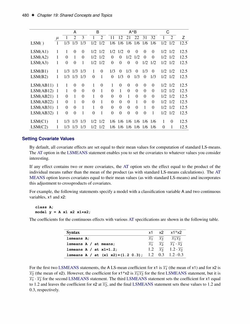
480 F Chapter 19: Shared Concepts and Topics
A B A*B C� 1 2 3 1 2 11 12 21 22 31 32 1 2 Z
LSM( ) 1 1/3 1/3 1/3 1/2 1/2 1/6 1/6 1/6 1/6 1/6 1/6 1/2 1/2 12.5
LSM(A1) 1 1 0 0 1/2 1/2 1/2 1/2 0 0 0 0 1/2 1/2 12.5LSM(A2) 1 0 1 0 1/2 1/2 0 0 1/2 1/2 0 0 1/2 1/2 12.5LSM(A3) 1 0 0 1 1/2 1/2 0 0 0 0 1/2 1/2 1/2 1/2 12.5
LSM(B1) 1 1/3 1/3 1/3 1 0 1/3 0 1/3 0 1/3 0 1/2 1/2 12.5LSM(B2) 1 1/3 1/3 1/3 0 1 0 1/3 0 1/3 0 1/3 1/2 1/2 12.5
LSM(AB11) 1 1 0 0 1 0 1 0 0 0 0 0 1/2 1/2 12.5LSM(AB12) 1 1 0 0 0 1 0 1 0 0 0 0 1/2 1/2 12.5LSM(AB21) 1 0 1 0 1 0 0 0 1 0 0 0 1/2 1/2 12.5LSM(AB22) 1 0 1 0 0 1 0 0 0 1 0 0 1/2 1/2 12.5LSM(AB31) 1 0 0 1 1 0 0 0 0 0 1 0 1/2 1/2 12.5LSM(AB32) 1 0 0 1 0 1 0 0 0 0 0 1 1/2 1/2 12.5
LSM(C1) 1 1/3 1/3 1/3 1/2 1/2 1/6 1/6 1/6 1/6 1/6 1/6 1 0 12.5LSM(C2) 1 1/3 1/3 1/3 1/2 1/2 1/6 1/6 1/6 1/6 1/6 1/6 0 1 12.5
Setting Covariate Values
By default, all covariate effects are set equal to their mean values for computation of standard LS-means.The AT option in the LSMEANS statement enables you to set the covariates to whatever values you considerinteresting.
If any effect contains two or more covariates, the AT option sets the effect equal to the product of theindividual means rather than the mean of the product (as with standard LS-means calculations). The ATMEANS option leaves covariates equal to their mean values (as with standard LS-means) and incorporatesthis adjustment to crossproducts of covariates.
For example, the following statements specify a model with a classification variable A and two continuousvariables, x1 and x2:
class A;model y = A x1 x2 x1*x2;
The coefficients for the continuous effects with various AT specifications are shown in the following table.
Syntax x1 x2 x1*x2lsmeans A; x1 x2 x1x2
lsmeans A / at means; x1 x2 x1 � x2
lsmeans A / at x1=1.2; 1.2 x2 1:2 � x2
lsmeans A / at (x1 x2)=(1.2 0.3); 1.2 0.3 1:2 � 0:3
For the first two LSMEANS statements, the A LS-mean coefficient for x1 is x1 (the mean of x1) and for x2 isx2 (the mean of x2). However, the coefficient for x1*x2 is x1x2 for the first LSMEANS statement, but it isx1 � x2 for the second LSMEANS statement. The third LSMEANS statement sets the coefficient for x1 equalto 1.2 and leaves the coefficient for x2 at x2, and the final LSMEANS statement sets these values to 1.2 and0.3, respectively.

Construction of Least Squares Means F 481
The covariate means used in computing the LS-means are affected by the AT option in the LSMEANSstatement as follows:
� If you use a WEIGHT statement:
– If you do not specify the AT option, unweighted covariate means are used for the covariatecoefficients.
– If you specify the AT option, weighted covariate means are used for the covariate coefficientsfor which no explicit AT values are specified (thus for all the covariate means if you specify ATMEANS).
� If any observations have missing dependent variable values:
– If you do not specify the AT option, these observations are not included in computing the covariatemeans.
– If you specify the AT option, these observations are included unless they form a missing cell (acombination of CLASS variables all of whose responses are missing).
These conditions are summarized in Table 19.22. You can use the E option in conjunction with the AT optionto verify that the modified LS-means coefficients are the ones you want.
Table 19.22 Treatment of Covariate Means with and without the AT Option
Without AT With ATWEIGHT statement Weights not used Weights usedObservations with missingdependent variable values
Observations not included Observations included
The AT option is disabled if you specify the BYLEVEL option, in which case the coefficients for thecovariates are set equal to their means within each level of the LS-mean effect in question.
Changing the Weighting Scheme
The standard LS-means have equal coefficients across classification effects; however, the OBSMARGINSoption in the LSMEANS statement changes these coefficients to be proportional to those found in the specifieddata set, or in the input data set if you do not specify a data set for observed margins. This adjustment isreasonable when you want your inferences to apply to a population that is not necessarily balanced but hasthe margins observed in the specified data set.
The computation of observed margins uses all observations for which there are no missing independentvariables, including those for which there are missing dependent variables. Also, if there is a WEIGHTvariable, weighted margins are used to construct the LS-means coefficients. If the observed margins data set isbalanced or if you specify a simple one-way model, the LS-means will be unchanged by the OBSMARGINSoption.
The BYLEVEL option modifies the observed-margins LS-means. Instead of computing the margins acrossthe entire data set, separate margins are computed for each level of the LS-mean effect in question. Theresulting LS-means are actually equal to raw means in this case. The BYLEVEL option disables the AToption if it is specified.

482 F Chapter 19: Shared Concepts and Topics
You might want to use the E option in conjunction with either the OBSMARGINS or BYLEVEL optionto verify that the modified LS-means coefficients are the ones you want. It is possible that the modifiedLS-means are not estimable when the standard ones are, or vice versa.
Estimability of LS-Means
LS-means are defined as certain linear combinations of the parameters. As such, it is possible for them to beinestimable. In fact, it is possible for a pair of LS-means to be both inestimable but their difference estimable.When this happens, only the entries that correspond to the estimable difference are computed and displayedin the Diffs table. If ADJUST=SIMULATE is specified when there are inestimable LS-means differences,adjusted results for all differences are displayed as missing.
ODS Table Names: LSMEANS StatementEach table created by the LSMEANS statement has a name associated with it, and you can use this name torefer to the table when using the Output Delivery System (ODS) to select tables and create output data sets.These names are listed in Table 19.23. For more information about ODS, see Chapter 20, “Using the OutputDelivery System.”
Table 19.23 ODS Tables Produced by the LSMEANS statement
Table Name Description Required Option
Coef L matrix coefficients EDiffs Differences of LS-means DIFF or ADJUST= or
STEPDOWNLSMeans LS-means DefaultLSMLines Lines display for LS-means LINES
ODS Graphics: LSMEANS StatementThis section describes the use of ODS Graphics for creating graphics that are related to LS-means inprocedures that support the common LSMEANS or SLICE statement. There are two groups of availableplots: those that can be produced by all procedures that support these two statements, and those that can beproduced only in association with the three procedures that can perform Bayesian analysis (PROC GENMOD,PROC LIFEREG, and PROC PHREG). Plots that are associated with the Bayesian analysis are availablevia these procedures directly, and also by using PROC PLM with an item store that was created by theseprocedures.
Plots in the first group depict the LS-means and their differences; when LS-mean comparisons are adjustedfor multiplicity by using the ADJUST= option, the plots are adjusted accordingly. To request plots in thisgroup, ODS Graphics must be enabled and you must request plots with the appropriate PLOTS= option inthe LSMEANS or SLICE statement. Plots in the second group depict the posterior sample distribution ofLS-means and their differences. To request plots in this group, you must also use a BAYES statement with
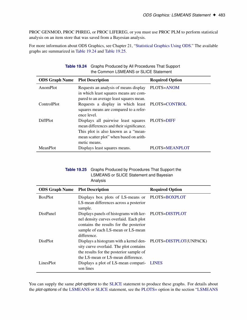
ODS Graphics: LSMEANS Statement F 483
PROC GENMOD, PROC PHREG, or PROC LIFEREG, or you must use PROC PLM to perform statisticalanalysis on an item store that was saved from a Bayesian analysis.
For more information about ODS Graphics, see Chapter 21, “Statistical Graphics Using ODS.” The availablegraphs are summarized in Table 19.24 and Table 19.25.
Table 19.24 Graphs Produced by All Procedures That Supportthe Common LSMEANS or SLICE Statement
ODS Graph Name Plot Description Required Option
AnomPlot Requests an analysis of means displayin which least squares means are com-pared to an average least squares mean.
PLOTS=ANOM
ControlPlot Requests a display in which leastsquares means are compared to a refer-ence level.
PLOTS=CONTROL
DiffPlot Displays all pairwise least squaresmean differences and their significance.This plot is also known as a “mean-mean scatter plot” when based on arith-metic means.
PLOTS=DIFF
MeanPlot Displays least squares means. PLOTS=MEANPLOT
Table 19.25 Graphs Produced by Procedures That Support theLSMEANS or SLICE Statement and BayesianAnalysis
ODS Graph Name Plot Description Required Option
BoxPlot Displays box plots of LS-means orLS-mean differences across a posteriorsample.
PLOTS=BOXPLOT
DistPanel Displays panels of histograms with ker-nel density curves overlaid. Each plotcontains the results for the posteriorsample of each LS-mean or LS-meandifference.
PLOTS=DISTPLOT
DistPlot Displays a histogram with a kernel den-sity curve overlaid. The plot containsthe results for the posterior sample ofthe LS-mean or LS-mean difference.
PLOTS=DISTPLOT(UNPACK)
LinesPlot Displays a plot of LS-mean compari-son lines
LINES
You can supply the same plot-options to the SLICE statement to produce these graphs. For details aboutthe plot-options of the LSMEANS or SLICE statement, see the PLOTS= option in the section “LSMEANS

484 F Chapter 19: Shared Concepts and Topics
Statement” on page 464. For more details about the DIFFPLOT in particular, see the section “Graphics forLS-Mean Comparisons” on page 3573 in Chapter 47, “The GLIMMIX Procedure.”
LSMESTIMATE Statement
This statement documentation applies to the following SAS/STAT procedures:GEE, GENMOD, LIFEREG, LOGISTIC, MIXED, ORTHOREG, PHREG, PLM, PROBIT, SURVEYLO-GISTIC, SURVEYPHREG, and SURVEYREG. It also applies to the RELIABILITY procedure in SAS/QCsoftware. The LSMESTIMATE statement in the GLIMMIX procedure is documented in Chapter 47, “TheGLIMMIX Procedure.”
The LSMESTIMATE statement provides a mechanism for obtaining custom hypothesis tests among leastsquares means. In contrast to the LSMEANS statement, the LSMESTIMATE statement does not produce theleast squares means or their differences; instead, you can estimate any linear function of the least squaresmeans (including the means themselves or their differences). In contrast to the linear functions that areconstructed with the ESTIMATE statement, you do not specify coefficients for the individual parameterestimates. Instead, with the LSMESTIMATE statement you specify coefficients for the least squares means;these are then converted for you into estimable functions for the parameter estimates.
The LSMESTIMATE statement thus combines important and convenient features of the LSMEANS and theESTIMATE statement. As with the LSMEANS statement, the following conditions are true:
� You need to specify only a single effect; the mapping into linear estimable functions in terms of theparameter estimates is performed by the procedure.
� You can use the AT=, BYLEVEL, and OBSMARGINS options to affect the computation of theunderlying least squares means.
As with the ESTIMATE statement you can do the following:
� specify multiple-row linear combinations.
� perform multiplicity corrections to control the familywise Type I error probability with the ADJUST=option.
� construct general linear functions of the least squares means.
� perform joint F or chi-square tests with or without order restrictions through the JOINT option.
� rely on positional or nonpositional syntax to specify coefficients for linear functions. For details aboutusing nonpositional syntax, see the section “Positional and Nonpositional Syntax for Coefficients inLinear Functions” on page 459.
The computation of an LSMESTIMATE involves two coefficient matrices. Suppose that there are nl levelsfor a valid least squares means effect (an effect that is part of your model and consists of classification

Syntax: LSMESTIMATE Statement F 485
variables only). Then the LS-means are formed as L1b, where L1 is a .nl � p/ coefficient matrix. The
.k � nl/ coefficient matrix K is formed from the values that you supply in the k rows of the LSMESTIMATEstatement. The least squares means estimates then represent the .k � 1/ vector
KL1ˇ D Lˇ
Because the analytic features and capabilities of the LSMESTIMATE statement are an amalgam of theLSMEANS and the ESTIMATE statement, the syntax of the statement follows the same pattern.
Syntax: LSMESTIMATE StatementLSMESTIMATE model-effect < 'label ' > values < DIVISOR=n >
< , < 'label ' > values < DIVISOR=n > > < , . . . >< / options > ;
In contrast to a multirow estimate in the ESTIMATE statement, you specify only a single effect in theLSMESTIMATE statement. The row labels are optional and follow the model-effect specification. Forexample, the following statements fit a split-split-plot design and compare the average of the third and fourthLS-mean of the whole-plot factor A to the first LS-mean of the factor:
proc glimmix;class a b block;model y = a b a*b / s;random int a / sub=block;lsmestimate A 'a1 vs avg(a3,a4)' 2 0 -1 -1 divisor=2;
run;
The order in which coefficients are assigned to the least squares means corresponds to the order in whichthey are displayed in the “Least Squares Means” table. You can use the ELSM option to see how coefficientsare matched to levels of the fixed effect.
The optional DIVISOR=n specification enables you to assign a separate divisor to each row of the LSMES-TIMATE. You can also assign divisor values through the DIVISOR= option. See the description of theDIVISOR= option that follows for the interaction between the two ways of specifying divisors.
Table 19.26 summarizes important options in the LSMESTIMATE statement. All LSMESTIMATE optionsare subsequently discussed in alphabetical order.
Table 19.26 LSMESTIMATE Statement Options
Option Description
Construction and Computation of LS-MeansAT Modifies covariate values in computing LS-meansBYLEVEL Computes separate marginsDIVISOR= Specifies a list of values to divide the coefficientsOM= Specifies the weighting scheme for LS-means computation as
determined by a data setSINGULAR= Tunes estimability checking

486 F Chapter 19: Shared Concepts and Topics
Table 19.26 continued
Option Description
Degrees of Freedom and p-valuesADJUST= Determines the method for multiple-comparison adjustment of
LS-means differencesALPHA=˛ Determines the confidence level (1 � ˛)LOWER Performs one-sided, lower-tailed inferenceSTEPDOWN Adjusts multiple-comparison p-values further in a step-down
fashionTESTVALUE= Specifies values under the null hypothesis for testsUPPER Performs one-sided, upper-tailed inference
Statistical OutputCL Constructs confidence limits for means and mean differencesCORR Displays the correlation matrix of LS-meansCOV Displays the covariance matrix of LS-meansE Prints the L matrixELSM Prints the K matrixJOINT Produces a joint F or chi-square test for the LS-means and
LS-means differencesPLOTS= Requests graphs of means and mean comparisonsSEED= Specifies the seed for computations that depend on random
numbers
Generalized Linear ModelingCATEGORY= Specifies how to construct estimable functions with multinomial
dataEXP Exponentiates and displays LS-means estimatesILINK Computes and displays estimates and standard errors of LS-means
(but not differences) on the inverse linked scale
You can specify the following options in the LSMESTIMATE statement after a slash (/):
ADJDFE=SOURCE
ADJDFE=ROWspecifies how denominator degrees of freedom are determined when p-values and confidence limitsare adjusted for multiple comparisons with the ADJUST= option. When you do not specify theADJDFE= option or when you specify ADJDFE=SOURCE, the denominator degrees of freedom formultiplicity-adjusted results are the denominator degrees of freedom for the LS-mean effect in the“Type III Tests of Fixed Effects” table.
The ADJDFE=ROW setting is useful if you want multiplicity adjustments to take into account thatdenominator degrees of freedom are not constant across estimates. For example, this can be thecase when the denominator degrees of freedom are computed by the Satterthwaite or Kenward-Rogermethod (Kenward and Roger 1997) in a mixed model.

Syntax: LSMESTIMATE Statement F 487
The ADJDFE= option is not supported by the procedures that perform chi-square-based inference(GENMOD, LOGISTIC, PHREG and SURVEYLOGISTIC).
ADJUST=BON
ADJUST=SCHEFFE
ADJUST=SIDAK
ADJUST=SIMULATE< (sim-options) >
ADJUST=Trequests a multiple comparison adjustment for the p-values and confidence limits for the LS-meanestimates. The adjusted quantities are produced in addition to the unadjusted p-values and confidencelimits. Adjusted confidence limits are produced if the CL or ALPHA= option is in effect. Fora description of the adjustments, see Chapter 48, “The GLM Procedure,” and Chapter 81, “TheMULTTEST Procedure,” in addition to the documentation for the ADJUST= option in the LSMEANSstatement.
Not all adjustment methods of the LSMEANS statement are available for the LSMESTIMATE state-ment. Multiplicity adjustments in the LSMEANS statement are designed specifically for differences ofleast squares means.
If you specify the STEPDOWN option, the p-values are further adjusted in a step-down fashion.
ALPHA=numberrequests that a t type confidence interval be constructed for each of the LS-means with confidence level1 – number . The value of number must be between 0 and 1; the default is 0.05.
AT variable=value
AT (var-list)=(value-list)
AT MEANSmodifies the values of the covariates used in computing LS-means. See the AT option in the LSMEANSstatement for details.
BYLEVELrequests that the procedure compute separate margins for each level of the LSMEANS effect.
The standard LS-means have equal coefficients across classification effects. The BYLEVEL optionchanges these coefficients to be proportional to the observed margins. This adjustment is reasonablewhen you want your inferences to apply to a population that is not necessarily balanced but has themargins observed in the input data set. In this case, the resulting LS-means are actually equal toraw means for fixed-effects models and certain balanced random-effects models, but their estimatedstandard errors account for the covariance structure that you have specified. If a WEIGHT statement isspecified, the procedure uses weighted margins to construct the LS-means coefficients.
If the AT option is specified, the BYLEVEL option disables it.
CATEGORY=category-optionsspecifies how to construct estimates and multiplicity corrections for models with multinomial data(ordinal or nominal). This option is also important for constructing sets of estimable functions for Ftests with the JOINT option.
The category-options indicate how response variable levels are treated in constructing the estimablefunctions. Possible value for the category-options are the following:
488 F Chapter 19: Shared Concepts and Topics
JOINTcomputes the estimable functions for every nonredundant category and treats them as a set. Forexample, a three-row LSMESTIMATE statement in a model with three response categories leadsto six estimable functions.
SEPARATEcomputes the estimable functions for every nonredundant category in turn. For example, athree-row LSMESTIMATE statement in a model with three response categories leads to two setsof three estimable functions.
quoted-value-listcomputes the estimable functions only for the specified list of values. The list must consist offormatted values of the response categories.
For further details about using the CATEGORY= option in models for multinomial data, see thedocumentation for the CATEGORY= option in the ESTIMATE statement.
The CATEGORY= option is supported only by the procedures that support generalized linear modeling(GEE, GENMOD, LOGISTIC, and SURVEYLOGISTIC) and by PROC PLM when it is used toperform statistical analyses on item stores that were created by these procedures.
CHISQrequests that chi-square tests be performed in addition to F tests, when you request an F test with theJOINT option. This option has no effect in procedures that produce chi-square statistics by default.
CLrequests that t type confidence limits be constructed for each of the LS-means. The confidence level is0.95 by default; this can be changed with the ALPHA= option. If you specify an ADJUST= option,then the confidence limits are adjusted for multiplicity. But if you also specify STEPDOWN, then onlyp-values are step-down adjusted, not the confidence limits.
CORRdisplays the estimated correlation matrix of the linear combination of the least squares means.
COVdisplays the estimated covariance matrix of the linear combination of the least squares means.
DF=numberspecifies the degrees of freedom for the tests and confidence limits. The option is not supportedby the procedures that perform chi-square-based inference (GENMOD, LOGISTIC, PHREG, andSURVEYLOGISTIC).
DIVISOR=value-listspecifies a list of values by which to divide the coefficients so that fractional coefficients can be enteredas integer numerators. If you do not specify value-list , a default value of 1.0 is assumed. Missingvalues in the value-list are converted to 1.0.
If the number of elements in value-list exceeds the number of rows of the estimate, the extra values areignored. If the number of elements in value-list is less than the number of rows of the estimate, the lastvalue in value-list is carried forward.
If you specify a row-specific divisor as part of the specification of the estimate row, this value multipliesthe corresponding value in the value-list . For example, the following statement divides the coefficientsin the first row by 8, and the coefficients in the third and fourth row by 3:

Syntax: LSMESTIMATE Statement F 489
lsmestimate A 'One vs. two' 8 -8 divisor=2,'One vs. three' 1 0 -1 ,'One vs. four' 3 0 0 -3 ,'One vs. five' 3 0 0 0 -3 / divisor=4,.,3;
Coefficients in the second row are not altered.
Erequests that the L coefficients of the estimable function be displayed. These are the coefficients thatapply to the fixed-effect parameter estimates. The E option displays the coefficients that you wouldneed to enter in an equivalent ESTIMATE statement.
ELSMrequests that the K matrix coefficients be displayed. These are the coefficients that apply to theLS-means. This option is useful to ensure that you assigned the coefficients correctly to the LS-means.
EXPrequests exponentiation of the least squares means estimate. When you model data with the logitlink function and the estimate represents a log odds ratio, the EXP option produces an odds ratio.If you specify the CL or ALPHA= option, the (adjusted) confidence limits for the estimate are alsoexponentiated.
The EXP option is supported only by PROC PHREG, PROC SURVEYPHREG, the procedures thatsupport generalized linear modeling (GEE, GENMOD, LOGISTIC, and SURVEYLOGISTIC), and byPROC PLM when it is used to perform statistical analyses on item stores that were created by theseprocedures.
ILINKrequests that the estimate and its standard error also be reported on the scale of the mean (the inverselinked scale). The computation of the inverse linked estimate depends on the estimation mode. Forexample, if the analysis is based on a posterior sample when a BAYES statement is present, theinversely linked estimate is the average of the inversely linked values across the sample of posteriorparameter estimates. If the analysis is not based on a sample of parameter estimates, the procedurecomputes the value on the mean scale by applying the inverse link to the estimate.
The interpretation of the inversely linked quantity depends on the coefficients that are specified in yourLSMESTIMATE statement and the link function. For example, in a model for binary data with logitlink the following LSMESTIMATE statement computes
q D1
1C expf�.�1 � �2/g
where �1 and �2 are the least squares means that are associated with the first two levels of theclassification effect A:
proc logistic;class A / param=glm;model y = A / dist=binary link=logit;lsmestimate A 1 -1 / ilink;
run;

490 F Chapter 19: Shared Concepts and Topics
The quantity q is not the difference of the probabilities associated with the two levels,
�1 � �2 D1
1C expf��1g�
1
1C expf��2g
The standard error of the inversely linked estimate is based on the delta method. If you also specify theCL or ALPHA= option, the procedure computes confidence intervals for the inversely linked estimate.These intervals are obtained by applying the inverse link to the confidence intervals on the linked scale.
The ILINK option is supported only by the procedures that support generalized linear modeling (GEE,GENMOD, LOGISTIC, and SURVEYLOGISTIC) and by PROC PLM when it is used to performstatistical analyses on item stores that were created by these procedures.
JOINT< (joint-test-options) >requests that a joint F or chi-square test be produced for the rows of the estimate. For more informationabout the simulation-based p-value calculation, see the section “Joint Hypothesis Tests with ComplexAlternatives, the Chi-Bar-Square Statistic” on page 461. You can specify the following joint-test-optionsin parentheses:
ACC= specifies the accuracy radius for determining the necessary sample size in the simulation-basedapproach of Silvapulle and Sen (2004) for tests with order restrictions. The value of must bestrictly between 0 and 1; the default value is 0.005.
EPS=�specifies the accuracy confidence level for determining the necessary sample size in the simulation-based approach of Silvapulle and Sen (2004) for F tests with order restrictions. The value of �must be strictly between 0 and 1; the default value is 0.01.
LABEL='label 'assigns an identifying label to the joint test. If you do not specify a label, the first non-defaultlabel for the ESTIMATE rows is used to label the joint test.
NOEST
ONLYperforms only the joint test and suppresses other results from the ESTIMATE statement. Thisoption is useful for emulating the CONTRAST statement that is available in other procedures.
NSAMP=nspecifies the number of samples for the simulation-based method of Silvapulle and Sen (2004).If n is not specified, it is constructed from the values of the ALPHA=˛, the ACC= , and theEPS=� options. With the default values for , �, and ˛ (0.005, 0.01, and 0.05, respectively),NSAMP=12,604 by default.
CHISQadds a chi-square test if the procedure produces an F test by default.
BOUNDS=value-listspecifies boundary values for the estimable linear function. The null value of the hypothesisis always zero. If you specify a positive boundary value z, the hypotheses are H W � D 0,HaW W � > 0 with the added constraint that � < z. The same is true for negative boundary values.

Syntax: LSMESTIMATE Statement F 491
The alternative hypothesis is then HaW � < 0 subject to the constraint � > �jzj. If you specify amissing value, the hypothesis is assumed to be two-sided. The BOUNDS option enables you tospecify sets of one- and two-sided joint hypotheses. If all values in value-list are set to missing,the procedure performs a simulation-based p-value calculation for a two-sided test.
LOWER
LOWERTAILEDrequests that the p-value for the t test be based only on values that are less than the test statistic. Atwo-tailed test is the default. A lower-tailed confidence limit is also produced if you specify the CL orALPHA= option.
Note that for ADJUST=SCHEFFE the one-sided adjusted confidence intervals and one-sided adjustedp-values are the same as the corresponding two-sided statistics, because this adjustment is based ononly the right tail of the F distribution.
If you request an F test with the JOINT option, then a one-sided left-tailed order restriction is appliedto all estimable functions, and the corresponding chi-bar-square statistic of Silvapulle and Sen (2004)is computed in addition to the two-sided, standard, F or chi-square statistic. See the JOINT option forhow to control the computation of the simulation-based chi-bar-square statistic.
OBSMARGINS< =OM-data-set >
OM< =OM-data-set >specifies a potentially different weighting scheme for the computation of LS-means coefficients. Thestandard LS-means have equal coefficients across classification effects; however, the OM optionchanges these coefficients to be proportional to those found in the OM-data-set . This adjustment isreasonable when you want your inferences to apply to a population that is not necessarily balanced buthas the margins observed in OM-data-set . See the OBSMARGINS option in the LSMEANS statementfor further details.
PLOTS=plot-optionsproduces ODS statistical graphics of the distribution of estimable functions if the procedure performsthe analysis in a sampling-based mode. For example, this is the case when procedures support aBAYES statement and perform a Bayesian analysis. The estimable functions are then computed foreach of the posterior parameter estimates, and the “Least Squares Means Estimates” table reportssimple descriptive statistics for the evaluated functions. In this situation, the PLOTS= option enablesyou to visualize the distribution of the estimable function. The following plot-options are available:
ALLproduces all possible plots with their default settings.
BOXPLOT< (boxplot-options) >produces box plots of the distribution of the estimable function across the posterior sample. Aseparate box plot is generated for each estimable function and all box plots appear on a singlegraph by default. You can affect the appearance of the box plot graph with the following options:
ORIENTATION=VERTICAL | HORIZONTAL
ORIENT=VERT | HORIZspecifies the orientation of the boxes. The default is vertical orientation of the box plots.

492 F Chapter 19: Shared Concepts and Topics
NPANELPOS=numberspecifies how to break the series of box plots across multiple panels. If the NPANELPOSoption is not specified, or if number equals zero, then all box plots are displayed in a singlegraph; this is the default. If a negative number is specified, then exactly up to jnumber j ofbox plots are displayed per panel. If number is positive, then the number of boxes per panelis balanced to achieve small variation in the number of box plots per graph.
DISTPLOT< (distplot-options) >
DIST< (distplot-options) >generates panels of histograms with a kernel density overlaid. A separate plot in each panelcontains the results for each estimable function. You can specify the following distplot-options inparentheses:
BOX | NOBOXcontrols the display of a horizontal box plot below the histogram. The BOX option is enabledby default.
HIST | NOHISTcontrols the display of the histogram of the estimable function’s distribution across theposterior sample. The HIST option is enabled by default.
NORMAL | NONORMALcontrols the display of a normal density estimate on the graph. The NONORMAL option isenabled by default.
KERNEL | NOKERNELcontrols the display of a kernel density estimate on the graph. The KERNEL option isenabled by default.
NROWS=numberspecifies the highest number of rows in a panel. The default is 3.
NCOLS=numberspecifies the highest number of columns in a panel. The default is 3.
UNPACKunpacks the panel into separate graphics.
NONEdoes not produce any plots.
SEED=numberspecifies the seed for the sampling-based components of the computations for the LSMESTIMATEstatement (for example, chi-bar-square statistics and simulated p-values). The value of number mustbe an integer. The seed is used to start the pseudo-random-number generator for the simulation. If youdo not specify a seed, or if you specify a value less than or equal to zero, the seed is generated fromreading the time of day from the computer clock. Note that there could be multiple LSMESTIMATEstatements with SEED= specifications and there could be other statements that can supply a randomnumber seed. Since the procedure has only one random number stream, the initial seed is shown in theSAS log.

Syntax: LSMESTIMATE Statement F 493
SINGULAR=numbertunes the estimability checking as documented for the SINGULAR= option in the ESTIMATE state-ment.
STEPDOWN< (step-down-options) >requests that multiplicity adjustments for the p-values of estimable functions be further adjustedin a step-down fashion. Step-down methods increase the power of multiple testing procedures bytaking advantage of the fact that a p-value is never declared significant unless all smaller p-values arealso declared significant. The STEPDOWN adjustment combined with ADJUST=BON correspondsto the methods of Holm (1979) and “Method 2” of Shaffer (1986); this is the default. Using step-down-adjusted p-values combined with ADJUST=SIMULATE corresponds to the method of Westfall(1997).
If the ESTIMATE statement is applied with a STEPDOWN option in a mixed model where the degrees-of-freedom method is that of Kenward and Roger (1997) or of Satterthwaite, then step-down-adjustedp-values are produced only if the ADJDFE=ROW option is in effect.
Also, the STEPDOWN option affects only p-values, not confidence limits. For ADJUST=SIMULATE,the generalized least squares hybrid approach of Westfall (1997) is used to increase Monte Carloaccuracy.
You can specify the following step-down-options in parentheses:
MAXTIME=nspecifies the time (in seconds) to be spent computing the maximal logically consistent sequentialsubsets of equality hypotheses for TYPE=LOGICAL. The default is MAXTIME=60. If theMAXTIME value is exceeded, the adjusted tests are not computed. When this occurs, you cantry increasing the MAXTIME value. However, note that there are common multiple comparisonsproblems for which this computation requires a huge amount of time—for example, all pairwisecomparisons between more than 10 groups. In such cases, try to use TYPE=FREE (the default)or TYPE=LOGICAL(n) for small n.
ORDER=PVALUE
ORDER=ROWSspecifies the order in which the step-down tests are performed. ORDER=PVALUE is the default,with LS-mean estimates being declared significant only if all LS-mean estimates with smaller(unadjusted) p-values are significant. If you specify ORDER=ROWS, then significances areevaluated in the order in which they are specified.
REPORTspecifies that a report on the step-down adjustment be displayed, including a listing of thesequential subsets (Westfall 1997) and, for ADJUST=SIMULATE, the step-down simulationresults.
TYPE=LOGICAL< (n) >
TYPE=FREEspecifies how step-down adjustment are made. If you specify TYPE=LOGICAL, the step-downadjustments are computed by using maximal logically consistent sequential subsets of equalityhypotheses (Shaffer 1986; Westfall 1997). Alternatively, for TYPE=FREE, sequential subsetsare computed ignoring logical constraints. The TYPE=FREE results are more conservative thanthose for TYPE=LOGICAL, but they can be much more efficient to produce for many estimates.

494 F Chapter 19: Shared Concepts and Topics
For example, it is not feasible to take logical constraints between all pairwise comparisons ofmore than about 10 groups. For this reason, TYPE=FREE is the default.
However, you can reduce the computational complexity of taking logical constraints into accountby limiting the depth of the search tree used to compute them, specifying the optional depthparameter as a number n in parentheses after TYPE=LOGICAL. As with TYPE=FREE, resultsfor TYPE=LOGICAL(n) are conservative relative to the true TYPE=LOGICAL results. But evenfor TYPE=LOGICAL(0), they can be appreciably less conservative than TYPE=FREE, and theyare computationally feasible for much larger numbers of estimates. If you do not specify n or if n= –1, the full search tree is used.
TESTVALUE=value-list
TESTMEAN=value-listspecifies the value under the null hypothesis for testing the estimable functions in the LSMESTIMATEstatement. The rules for specifying the value-list are very similar to those for specifying the divisorlist in the DIVISOR= option. If no TESTVALUE= is specified, all tests are performed as H WLˇ D 0.Missing values in the value-list also are translated to zeros. If you specify fewer values than rows inthe LSMESTIMATE statement, the last value in value-list is carried forward.
The TESTVALUE= option affects only p-values from individual, joint, and multiplicity-adjusted tests.It does not affect confidence intervals.
The TESTVALUE option is not available for the multinomial distribution, and the values are ignoredwhen you perform a sampling-based (Bayesian) analysis.
UPPER
UPPERTAILEDrequests that the p-value for the t test be based only on values that are greater than the test statistic. Atwo-tailed test is the default. An upper-tailed confidence limit is also produced if you specify the CL orALPHA= option.
Note that for ADJUST=SCHEFFE the one-sided adjusted confidence intervals and one-sided adjustedp-values are the same as the corresponding two-sided statistics, because this adjustment is based ononly the right tail of the F distribution.
If you request a joint test with the JOINT option, then a one-sided right-tailed order restriction isapplied to all estimable functions, and the corresponding chi-bar-square statistic of Silvapulle and Sen(2004) is computed in addition to the two-sided, standard, F or chi-square statistic. See the JOINToption for how to control the computation of the simulation-based chi-bar-square statistic.
ODS Table Names: LSMESTIMATE StatementEach table created by the LSMESTIMATE statement has a name associated with it, and you can use thisname to refer to the table when using the Output Delivery System (ODS) to select tables and create outputdata sets. These names are listed in Table 19.27. For more information about ODS, see Chapter 20, “Usingthe Output Delivery System.”

ODS Graphics: LSMESTIMATE Statement F 495
Table 19.27 ODS Tables Produced by the LSMESTIMATEstatement
Table Name Description Required Option
Coef L matrix coefficients or K matrix coef-ficients
E or ELSM
LSMEstimates Estimates among LS-means DefaultContrasts Joint test results for LS-means esti-
matesJOINT
ODS Graphics: LSMESTIMATE StatementThis section describes the use of ODS for creating statistical graphs of the distribution of LS-means andLS-mean differences with the LSMESTIMATE statement. The plots can be produced only in associationwith the three procedures that can perform Bayesian analysis (PROC GENMOD, PROC LIFEREG, andPROC PHREG). The plots are available via these procedures directly, and also via PROC PLM when runusing an item store that was created by these procedures. To request these graphs, you must do the following:
� ensure that ODS Graphics is enabled
� use a BAYES statement with PROC GENMOD, PROC LIFEREG, or PROC PHREG, or use PROCPLM to perform statistical analysis on an item store that was saved from a Bayesian analysis
� request plots with the PLOTS= option in the LSMESTIMATE statement
For more information about ODS Graphics, see Chapter 21, “Statistical Graphics Using ODS.” The availablegraphs are summarized in Table 19.28.
Table 19.28 Graphs Produced by the LSMESTIMATE statement
ODS Graph Name Plot Description Required Option
BoxPlot Displays box plots of LS-means orLS-mean differences across a posteriorsample.
PLOTS=BOXPLOT
DistPanel Displays panels of histograms with ker-nel density curves overlaid. Each plotcontains the results for the posteriorsample of each LS-mean or LS-meandifference.
PLOTS=DISTPLOT
DistPlot Displays a histogram with a kernel den-sity curve overlaid. The plot containsthe results for the posterior sample ofthe LS-mean or LS-mean difference.
PLOTS=DISTPLOT(UNPACK)
496 F Chapter 19: Shared Concepts and Topics
For details about the plot-options of the LSMESTIMATE statement, see the PLOTS= option in the section“LSMESTIMATE Statement” on page 484.
NLOPTIONS Statement
This section applies to the following procedures:CALIS, GLIMMIX, HPMIXED, PHREG, SURVEYPHREG, and VARIOGRAM. See the individual proce-dure chapters for deviations from the common syntax and defaults shown here.
Syntax: NLOPTIONS StatementThe NLOPTIONS statement provides you with syntax to control aspects of the nonlinear optimizations in theCALIS, GLIMMIX, HPMIXED, PHREG, SURVEYPHREG, and VARIOGRAM procedures.
NLOPTIONS < options > ;
The nonlinear optimization options are described in alphabetical order after Table 19.29, which summarizesthe options by category. The notation used in describing the options is generic in the sense that denotesthe p � 1 vector of parameters for the optimization and i is its ith element. The objective function beingminimized, its p � 1 gradient vector, and its p � p Hessian matrix are denoted as f . /, g. /, and H. /,respectively. The gradient with respect to the ith parameter is denoted as gi . /. Superscripts in parenthesesdenote the iteration count; for example, f . /.k/ is the value of the objective function at iteration k. In themixed model procedures, the parameter vector might consist of fixed effects only, covariance parametersonly, or fixed effects and covariance parameters. In the CALIS procedure, consists of all independentparameters that are defined in the models and in the PARAMETERS statement.
Table 19.29 Options to Control Aspects of the Optimization
Option Description
OptimizationHESCAL= Determines the type of Hessian scalingINHESSIAN= Specifies the start for approximated HessianLINESEARCH= Specifies the line-search methodLSPRECISION= Specifies the line-search precisionRESTART= Specifies the iteration number for update restartTECHNIQUE= Determines the minimization techniqueUPDATE= Determines the update technique
Termination CriteriaABSCONV= Tunes an absolute function convergence criterionABSFCONV= Tunes an absolute function difference convergence criterionABSGCONV= Tunes the absolute gradient convergence criterionABSXCONV= Tunes the absolute parameter convergence criterion

Syntax: NLOPTIONS Statement F 497
Table 19.29 continued
Option Description
FCONV= Tunes the relative function convergence criterionFCONV2= Tunes another relative function convergence criterionFSIZE= Specifies the value used in the FCONV and GCONV criteriaGCONV= Tunes the relative gradient convergence criterionGCONV2= Tunes another relative gradient convergence criterionMAXFUNC= Specifies the maximum number of function callsMAXITER= Specifies the maximum number of iterationsMAXTIME= Specifies the upper limit for seconds of CPU timeMINITER= Specifies the minimum number of iterationsXCONV= Specifies the relative parameter convergence criterionXSIZE= Specifies the value used in the XCONV criterion
Step LengthDAMPSTEP= Dampens steps in a line searchINSTEP= Specifies the initial trust region radiusMAXSTEP= Specifies the maximum trust region radius
Printed OutputPALL Displays (almost) all printed outputPHISTORY Displays optimization historyNOPRINT Suppresses all printed output
Covariance Matrix TolerancesASINGULAR= Specifies the absolute singularity for inertiaMSINGULAR= Specifies the relative M singularity for inertiaVSINGULAR= Specifies the relative V singularity for inertia
Constraint SpecificationsLCEPSILON= Specifies the range for active constraintsLCDEACT= Specifies the LM tolerance for deactivatingLCSINGULAR= Specifies the tolerance for dependent constraints
Remote MonitoringSOCKET= Specifies the fileref for remote monitoring
ABSCONV=r
ABSTOL=rspecifies an absolute function convergence criterion: for minimization, termination requires f . .k// �
r . The default value of r is the negative square root of the largest double-precision value, which servesonly as a protection against overflows.

498 F Chapter 19: Shared Concepts and Topics
ABSFCONV=r < n >
ABSFTOL=r< n >specifies an absolute function difference convergence criterion:
� For all techniques except NMSIMP (specified by the TECHNIQUE= option), termination requiresa small change of the function value in successive iterations,
jf . .k�1// � f . .k//j � r
� The same formula is used for the NMSIMP technique, but .k/ is defined as the vertex with thelowest function value, and .k�1/ is defined as the vertex with the highest function value in thesimplex.
The default value is r = 0. The optional integer value n specifies the number of successive iterationsfor which the criterion must be satisfied before the process can be terminated.
ABSGCONV=r < n >ABSGTOL=r< n >
specifies an absolute gradient convergence criterion:
� For all techniques except NMSIMP (specified by the TECHNIQUE= option), termination requiresthe maximum absolute gradient element to be small:
maxjjgj .
.k//j � r
� This criterion is not used by the NMSIMP technique.
The default value is r = 1E–5. The optional integer value n specifies the number of successive iterationsfor which the criterion must be satisfied before the process can be terminated.
ABSXCONV=r < n >ABSXTOL=r< n >
specifies an absolute parameter convergence criterion:
� For all techniques except NMSIMP, termination requires a small Euclidean distance betweensuccessive parameter vectors,
k .k/� .k�1/
k2� r
� For the NMSIMP technique, termination requires either a small length ˛.k/ of the vertices of arestart simplex,
˛.k/� r
or a small simplex size,
ı.k/� r
where the simplex size ı.k/ is defined as the L1 distance from the simplex vertex �.k/ with thesmallest function value to the other p simplex points .k/
l¤ �.k/:
ı.k/D
X l¤y
k .k/
l� �.k/
k1

Syntax: NLOPTIONS Statement F 499
The default is r = 1E–8 for the NMSIMP technique and r = 0 otherwise. The optional integer value nspecifies the number of successive iterations for which the criterion must be satisfied before the processcan terminate.
ASINGULAR=r
ASING=rspecifies an absolute singularity criterion for the computation of the inertia (number of positive,negative, and zero eigenvalues) of the Hessian and its projected forms. The default value is the squareroot of the smallest positive double-precision value.
DAMPSTEP< =r >specifies that the initial step length value ˛.0/ for each line search (used by the QUANEW, CONGRA,or NEWRAP technique) cannot be larger than r times the step length value used in the formeriteration. If the DAMPSTEP option is specified but r is not specified, the default is r = 2. TheDAMPSTEP= option can prevent the line-search algorithm from repeatedly stepping into regionswhere some objective functions are difficult to compute or where they could lead to floating-pointoverflows during the computation of objective functions and their derivatives. The DAMPSTEP=option can save time-consuming function calls during the line searches of objective functions thatresult in very small steps.
FCONV=r< n >
FTOL=r< n >specifies a relative function convergence criterion:
� For all techniques except NMSIMP, termination requires a small relative change of the functionvalue in successive iterations,
jf . .k// � f . .k�1//j
max.jf . .k�1//j;FSIZE/� r
where FSIZE is defined by the FSIZE= option.
� The same formula is used for the NMSIMP technique, but .k/ is defined as the vertex with thelowest function value and .k�1/ is defined as the vertex with the highest function value in thesimplex.
The default is r D 10�FDIGITS, where FDIGITS is by default � log10f�g and � is the machineprecision. Some procedures, such as the GLIMMIX procedure, enable you to change the value withthe FDIGITS= option in the PROC statement. The optional integer value n specifies the number ofsuccessive iterations for which the criterion must be satisfied before the process can terminate.
FCONV2=r< n >
FTOL2=r< n >specifies a second function convergence criterion:
� For all techniques except NMSIMP, termination requires a small predicted reduction,
df .k/� f . .k// � f . .k/
C s.k//
500 F Chapter 19: Shared Concepts and Topics
of the objective function. The predicted reduction
df .k/D �g.k/0
s.k/�1
2s.k/0
H.k/s.k/
D �1
2s.k/0
g.k/� r
is computed by approximating the objective function f by the first two terms of the Taylor seriesand substituting the Newton step,
s.k/D �ŒH.k/��1g.k/
� For the NMSIMP technique, termination requires a small standard deviation of the functionvalues of the p C 1 simplex vertices .k/
l, l D 0; : : : ; p,s
1
nC 1
Xl
hf .
.k/
l/ � f . .k//
i2� r
where f . .k// D 1pC1
Pl f .
.k/
l/. If there are pact boundary constraints active at .k/, the
mean and standard deviation are computed only for the nC 1 � pact unconstrained vertices.
The default value is r = 1E–6 for the NMSIMP technique and r= 0 otherwise. The optional integervalue n specifies the number of successive iterations for which the criterion must be satisfied beforethe process can terminate.
FSIZE=rspecifies the FSIZE parameter of the relative function and relative gradient termination criteria. Thedefault value is r = 0. For more details, see the FCONV= and GCONV= options.
GCONV=r< n >
GTOL=r< n >specifies a relative gradient convergence criterion:
� For all techniques except CONGRA and NMSIMP, termination requires that the normalizedpredicted function reduction be small,
g. .k//0ŒH.k/��1g. .k//
max.jf . .k//j;FSIZE/� r
where FSIZE is defined by the FSIZE= option. For the CONGRA technique (where a reliableHessian estimate H is not available), the following criterion is used:
k g. .k// k22 k s. .k// k2
k g. .k// � g. .k�1// k2 max.jf . .k//j;FSIZE/� r
� This criterion is not used by the NMSIMP technique.
The default value is r = 1E–8. The optional integer value n specifies the number of successive iterationsfor which the criterion must be satisfied before the process can terminate.

Syntax: NLOPTIONS Statement F 501
GCONV2=r< n >
GTOL2=r< n >specifies another relative gradient convergence criterion:
� For least squares problems and the TRUREG, LEVMAR, NRRIDG, and NEWRAP techniques,the following criterion of Browne (1982) is used:
maxj
jgj . .k//jq
f . .k//H.k/j;j
� r
� This criterion is not used by the other techniques.
The default value is r = 0. The optional integer value n specifies the number of successive iterationsfor which the criterion must be satisfied before the process can terminate.
HESCAL=0 | 1 | 2 | 3
HS=0 | 1 | 2 | 3specifies the scaling version of the Hessian (or crossproduct Jacobian) matrix used in NRRIDG,TRUREG, LEVMAR, NEWRAP, or DBLDOG optimization.
If HS is not equal to 0, the first iteration and each restart iteration set the diagonal scaling matrixD.0/ D diag.d .0/
i /:
d.0/i D
qmax.jH .0/
i;i j; �/
where H .0/i;i are the diagonal elements of the Hessian (or crossproduct Jacobian). In every other
iteration, the diagonal scaling matrix D.0/ D diag.d .0/i / is updated depending on the HS option:
0 specifies that no scaling be done.
1 specifies the Moré (1978) scaling update:
d.kC1/i D max
�d
.k/i ;
qmax.jH .k/
i;i j; �/
�2 specifies the Dennis, Gay, and Welsch (1981) scaling update:
d.kC1/i D max
�0:6 � d
.k/i ;
qmax.jH .k/
i;i j; �/
�3 specifies that di be reset in each iteration:
d.kC1/i D
qmax.jH .k/
i;i j; �/
In each scaling update, � is the relative machine precision. The default value is HS=0. Scaling of theHessian can be time-consuming in the case where general linear constraints are active.

502 F Chapter 19: Shared Concepts and Topics
INHESSIAN< =r >
INHESS< =r >specifies how the initial estimate of the approximate Hessian is defined for the quasi-Newton techniquesQUANEW and DBLDOG. There are two alternatives:
� If you do not use the r specification, the initial estimate of the approximate Hessian is set to theHessian at .0/.
� If you do use the r specification, the initial estimate of the approximate Hessian is set to themultiple of the identity matrix rI.
By default (if you do not specify the option INHESSIAN=r ), the initial estimate of the approximateHessian is set to the multiple of the identity matrix rI, where the scalar r is computed from themagnitude of the initial gradient.
INSTEP=r
SALPHA=r
RADIUS=rreduces the length of the first trial step during the line search of the first iterations. For highly nonlinearobjective functions, such as the EXP function, the default initial radius of the trust-region algorithmTRUREG or DBLDOG or the default step length of the line-search algorithms can result in arithmeticoverflows. If this occurs, you should specify decreasing values of 0 < r < 1 such as INSTEP=1E–1,INSTEP=1E–2, INSTEP=1E–4, and so on, until the iteration starts successfully.
� For trust-region algorithms (TRUREG or DBLDOG), the INSTEP= option specifies a factor r >0 for the initial radius �.0/ of the trust region. The default initial trust-region radius is the lengthof the scaled gradient. This step corresponds to the default radius factor of r = 1.
� For line-search algorithms (NEWRAP, CONGRA, or QUANEW), the INSTEP= option specifiesan upper bound for the initial step length for the line search during the first five iterations. Thedefault initial step length is r = 1.
� For the Nelder-Mead simplex algorithm, by using TECH=NMSIMP, the INSTEP=r option definesthe size of the start simplex.
LCDEACT=r
LCD=rspecifies a threshold r for the Lagrange multiplier that determines whether an active inequalityconstraint remains active or can be deactivated. For maximization, r must be greater than zero; forminimization, r must be smaller than zero. An active inequality constraint can be deactivated only ifits Lagrange multiplier is less than the threshold value. The default value is
r D ˙min.0:01;max.0:1 �ABSGCONV; 0:001 � gmax.k///
where “+” is for maximization, “–” is for minimization, ABSGCONV is the value of the absolutegradient criterion, and gmax.k/ is the maximum absolute element of the gradient or the projectedgradient.

Syntax: NLOPTIONS Statement F 503
LCEPSILON=rLCEPS=rLCE=r
specifies the range r for active and violated boundary constraints, where r � 0. If the point .k/
satisfies the following condition, the constraint i is recognized as an active constraint:
j
kXjD1
aij .k/j � bi j � r � .jbi j C 1/
Otherwise, the constraint i is either an inactive inequality or a violated inequality or equality constraint.The default value is r = 1E–8. During the optimization process, the introduction of rounding errors canforce the optimization to increase the value of r by a factor of 10k for some k > 0. If this happens, it isindicated by a message displayed in the log.
LCSINGULAR=rLCSING=rLCS=r
specifies a criterion r , where r � 0, that is used in the update of the QR decomposition and thatdetermines whether an active constraint is linearly dependent on a set of other active constraints. Thedefault value is r = 1E–8. The larger r becomes, the more the active constraints are recognized as beinglinearly dependent. If the value of r is larger than 0.1, it is reset to 0.1.
LINESEARCH=iLIS=i
specifies the line-search method for the CONGRA, QUANEW, and NEWRAP optimization techniques.See Fletcher (1987) for an introduction to line-search techniques. The value of i can be 1; : : : ; 8 asfollows. The default is LIS=2.
1 specifies a line-search method that needs the same number of function and gradientcalls for cubic interpolation and cubic extrapolation; this method is similar to oneused by the Harwell subroutine library.
2 specifies a line-search method that needs more function than gradient calls forquadratic and cubic interpolation and cubic extrapolation; this method is imple-mented as shown in Fletcher (1987) and can be modified to an exact line search byusing the LSPRECISION= option. This is the default.
3 specifies a line-search method that needs the same number of function and gradientcalls for cubic interpolation and cubic extrapolation; this method is implemented asshown in Fletcher (1987) and can be modified to an exact line search by using theLSPRECISION= option.
4 specifies a line-search method that needs the same number of function and gradientcalls for stepwise extrapolation and cubic interpolation.
5 specifies a line-search method that is a modified version of LIS=4.
6 specifies a golden-section line search (Polak 1971), which uses only function valuesfor linear approximation.
7 specifies a bisection line search (Polak 1971), which uses only function values forlinear approximation.
8 specifies the Armijo line-search technique (Polak 1971), which uses only functionvalues for linear approximation.

504 F Chapter 19: Shared Concepts and Topics
LSPRECISION=r
LSP=rspecifies the degree of accuracy that should be obtained by the line-search algorithms LIS=2 andLIS=3. Usually an imprecise line search is inexpensive and successful. For more difficult optimizationproblems, a more precise and expensive line search might be necessary (Fletcher 1987). The LIS=2line-search method (which is the default for the NEWRAP, QUANEW, and CONGRA techniques)and the LIS=3 line-search method approach exact line search for small LSPRECISION= values. Ifyou have numerical problems, try to decrease the LSPRECISION= value to obtain a more precise linesearch. The default values are shown in Table 19.30.
Table 19.30 Default Values for Line-Search Precision
TECH= UPDATE= LSP Default
QUANEW DBFGS, BFGS r = 0.4QUANEW DDFP, DFP r = 0.06CONGRA All r = 0.1NEWRAP No update r = 0.9
For more details, see Fletcher (1987).
MAXFUNC=i
MAXFU=ispecifies the maximum number i of function calls in the optimization process. The default values areas follows:
� 125 for the TRUREG, NRRIDG, NEWRAP, and LEVMAR techniques
� 500 for the QUANEW and DBLDOG techniques
� 1000 for the CONGRA technique
� 3000 for the NMSIMP technique
Optimization can terminate only after completing a full iteration. Therefore, the number of functioncalls that are actually performed can exceed the number that is specified by the MAXFUNC= option.
MAXITER=i
MAXIT=ispecifies the maximum number i of iterations in the optimization process. The default values are asfollows:
� 50 for the TRUREG, NRRIDG, NEWRAP, and LEVMAR techniques
� 200 for the QUANEW and DBLDOG techniques
� 400 for the CONGRA technique
� 1000 for the NMSIMP technique
These default values are also valid when i is specified as a missing value.
Syntax: NLOPTIONS Statement F 505
MAXSTEP=r< n >specifies an upper bound for the step length of the line-search algorithms during the first n iterations.By default, r is the largest double-precision value and n is the largest integer available. Setting thisoption can improve the speed of convergence for the CONGRA, QUANEW, and NEWRAP techniques.
MAXTIME=rspecifies an upper limit of r seconds of CPU time for the optimization process. The time specifiedby the MAXTIME= option is checked only once at the end of each iteration. Therefore, the actualrunning time can be much longer than that specified by the MAXTIME= option. The actual runningtime includes the rest of the time needed to finish the iteration and the time needed to generate theoutput of the results. By default, CPU time is not limited.
MINITER=i
MINIT=ispecifies the minimum number of iterations. The default value is 0. If you request more iterationsthan are actually needed for convergence to a stationary point, the optimization algorithms can behavestrangely. For example, the effect of rounding errors can prevent the algorithm from continuing for therequired number of iterations.
MSINGULAR=r
MSING=rspecifies a relative singularity criterion r , where r > 0, for the computation of the inertia (number ofpositive, negative, and zero eigenvalues) of the Hessian and its projected forms. The default value is1E–12.
NOPRINTsuppresses output that is related to optimization, such as the iteration history. This option, along withall NLOPTIONS statement options for displayed output, are ignored by the GLIMMIX and HPMIXEDprocedures.
PALLdisplays all optional output for optimization. This option is supported only by the CALIS andSURVEYPHREG procedures.
PHISTORY
PHISTdisplays the optimization history. The PHISTORY option is implied if the PALL option is specified.The PHISTORY option is supported only by the CALIS and SURVEYPHREG procedures.
RESTART=i
REST=ispecifies that the QUANEW or CONGRA technique is restarted with a steepest search direction afterat most i iterations, where i > 0. Default values are as follows:
� When TECHNIQUE=CONGRA and UPDATE=PB, restart is performed automatically; so i isnot used.
� When TECHNIQUE=CONGRA and UPDATE¤PB, i = min.10p; 80/, where p is the number ofparameters.
� When TECHNIQUE=QUANEW, i is the largest integer available.

506 F Chapter 19: Shared Concepts and Topics
SINGULAR=r
SING=rspecifies the singularity criterion r , 0 � r � 1, that is used for the inversion of the Hessian matrix. Thedefault value is 1E–8.
SOCKET=filerefspecifies the fileref that contains the information needed for remote monitoring.
TECHNIQUE=value
TECH=value
OMETHOD=value
OM=valuespecifies the optimization technique. You can find additional information about choosing an optimiza-tion technique in the section “Choosing an Optimization Algorithm” on page 508. Valid values for theTECHNIQUE= option are as follows:
� CONGRAperforms a conjugate-gradient optimization, which can be more precisely specified with theUPDATE= option and modified with the LINESEARCH= option. When you specify this option,UPDATE=PB by default.
� DBLDOGperforms a version of double-dogleg optimization, which can be more precisely specified withthe UPDATE= option. When you specify this option, UPDATE=DBFGS by default.
� LEVMARperforms a highly stable, but for large problems memory- and time-consuming, Levenberg-Marquardt optimization technique, a slightly improved variant of the Moré (1978) implementation.You can also specify this technique with the alias LM or MARQUARDT. In the CALIS procedure,this is the default optimization technique if there are fewer than 40 parameters to estimate. TheGLIMMIX and HPMIXED procedures do not support this optimization technique.
� NMSIMPperforms a Nelder-Mead simplex optimization. The CALIS procedure does not support thisoptimization technique.
� NONEdoes not perform any optimization. This option can be used for the following:
– to perform a grid search without optimization– to compute estimates and predictions that cannot be obtained efficiently with any of the
optimization techniques– to obtain inferences for known values of the covariance parameters
� NEWRAPperforms a Newton-Raphson optimization that combines a line-search algorithm with ridging.The line-search algorithm LIS=2 is the default method.
� NRRIDGperforms a Newton-Raphson optimization with ridging. This is the default optimization techniquein the SURVEYPHREG procedure.

Syntax: NLOPTIONS Statement F 507
� QUANEWperforms a quasi-Newton optimization, which can be defined more precisely with the UPDATE=option and modified with the LINESEARCH= option.
� TRUREGperforms a trust-region optimization.
UPDATE=method
UPD=methodspecifies the update method for the quasi-Newton, double-dogleg, or conjugate-gradient optimizationtechnique. Not every update method can be used with each optimizer.
The following are the valid methods for the UPDATE= option:
� BFGSperforms the original Broyden, Fletcher, Goldfarb, and Shanno (BFGS) update of the inverseHessian matrix.
� DBFGSperforms the dual BFGS update of the Cholesky factor of the Hessian matrix. This is the defaultupdate method.
� DDFPperforms the dual Davidon, Fletcher, and Powell (DFP) update of the Cholesky factor of theHessian matrix.
� DFPperforms the original DFP update of the inverse Hessian matrix.
� PBperforms the automatic restart update method of Powell (1977) and Beale (1972).
� FRperforms the Fletcher-Reeves update (Fletcher 1987).
� PRperforms the Polak-Ribiere update (Fletcher 1987).
� CDperforms a conjugate-descent update of Fletcher (1987).
VERSION=1 | 2
VS=1 | 2specifies the version of the quasi-Newton optimization technique with nonlinear constraints.
VS=1 specifies the update of the � vector as in Powell (1978b, a) (update like VF02AD).
VS=2 specifies the update of the � vector as in Powell (1982b, a) (update like VMCWD).
The default is VERSION=2.

508 F Chapter 19: Shared Concepts and Topics
VSINGULAR=r
VSING=rspecifies a relative singularity criterion r , where r > 0, for the computation of the inertia (number ofpositive, negative, and zero eigenvalues) of the Hessian and its projected forms. The default value is r= 1E–8.
XCONV=r< n >
XTOL=r< n >specifies the relative parameter convergence criterion:
� For all techniques except NMSIMP, termination requires a small relative parameter change insubsequent iterations:
maxj j .k/j �
.k�1/j j
max.j .k/j j; j
.k�1/j j;XSIZE/
� r
� For the NMSIMP technique, the same formula is used, but .k/j is defined as the vertex with the
lowest function value and .k�1/j is defined as the vertex with the highest function value in the
simplex.
The default value is r = 1E–8 for the NMSIMP technique and r = 0 otherwise. The optional integervalue n specifies the number of successive iterations for which the criterion must be satisfied beforethe process can be terminated.
XSIZE=rspecifies the XSIZE parameter r of the relative parameter termination criterion, where r � 0. Thedefault value is r = 0. For more details, see the XCONV= option.
Choosing an Optimization Algorithm
First- or Second-Order Algorithms
The factors that go into choosing a particular optimization technique for a particular problem are complex.Trial and error can be involved.
For many optimization problems, computing the gradient takes more computer time than computing thefunction value. Computing the Hessian sometimes takes much more computer time and memory thancomputing the gradient, especially when there are many decision variables. Unfortunately, optimizationtechniques that do not use some kind of Hessian approximation usually require many more iterations thantechniques that do use a Hessian matrix, and, as a result, the total run time of these techniques is often longer.Techniques that do not use the Hessian also tend to be less reliable. For example, they can terminate moreeasily at stationary points than at global optima.
Table 19.31 shows which derivatives are required for each optimization technique.

Choosing an Optimization Algorithm F 509
Table 19.31 Derivatives Required
Algorithm First-Order Second-Order
LEVMAR x xTRUREG x xNEWRAP x xNRRIDG x xQUANEW x -DBLDOG x -CONGRA x -NMSIMP - -
The second-derivative methods TRUREG, NEWRAP, and NRRIDG are best for small problems where theHessian matrix is not expensive to compute. Sometimes the NRRIDG algorithm can be faster than theTRUREG algorithm, but TRUREG can be more stable. The NRRIDG algorithm requires only one matrixwith p.p C 1/=2 double words; TRUREG and NEWRAP require two such matrices. Here, p denotes thenumber of parameters in the optimization.
The first-derivative methods QUANEW and DBLDOG are best for medium-sized problems where theobjective function and the gradient are much faster to evaluate than the Hessian. In general, the QUANEWand DBLDOG algorithms require more iterations than TRUREG, NRRIDG, and NEWRAP, but each iterationcan be much faster. The QUANEW and DBLDOG algorithms require only the gradient to update anapproximate Hessian, and they require slightly less memory than TRUREG or NEWRAP (essentially onematrix with p.p C 1/=2 double words).
The first-derivative method CONGRA is best for large problems where the objective function and thegradient can be computed much faster than the Hessian and where too much memory is required to storethe (approximate) Hessian. In general, the CONGRA algorithm requires more iterations than QUANEW orDBLDOG, but each iteration can be much faster. Because CONGRA requires only a factor of p double-wordmemory, many large applications can be solved only by CONGRA.
The no-derivative method NMSIMP is best for small problems where derivatives are not continuous or arevery difficult to compute.
Each optimization method uses one or more convergence criteria that determine when it has converged.An algorithm is considered to have converged when any one of the convergence criteria is satisfied. Forexample, under the default settings, the QUANEW algorithm will converge if ABSGCONV < 1E–5, FCONV< 10�FDIGITS, or GCONV < 1E–8.
Algorithm Descriptions
Trust Region Optimization (TRUREG)The trust region method uses the gradient g. .k// and the Hessian matrix H. .k//; thus, it requires that theobjective function f . / have continuous first- and second-order derivatives inside the feasible region.
The trust region method iteratively optimizes a quadratic approximation to the nonlinear objective functionwithin a hyperelliptic trust region with radius � that constrains the step size that corresponds to the quality ofthe quadratic approximation. The trust region method is implemented based on Dennis, Gay, and Welsch(1981); Gay (1983) and Moré and Sorensen (1983).

510 F Chapter 19: Shared Concepts and Topics
The trust region method performs well for small- to medium-sized problems, and it does not need manyfunction, gradient, and Hessian calls. However, if the computation of the Hessian matrix is computationallyexpensive, one of the (dual) quasi-Newton or conjugate gradient algorithms might be more efficient.
Newton-Raphson Optimization with Line Search (NEWRAP)The NEWRAP technique uses the gradient g. .k// and the Hessian matrix H. .k//; thus, it requires thatthe objective function have continuous first- and second-order derivatives inside the feasible region. Ifsecond-order derivatives are computed efficiently and precisely, the NEWRAP method can perform well formedium-sized to large problems, and it does not need many function, gradient, and Hessian calls.
This algorithm uses a pure Newton step when the Hessian is positive definite and when the Newton stepreduces the value of the objective function successfully. Otherwise, a combination of ridging and line searchis performed to compute successful steps. If the Hessian is not positive definite, a multiple of the identitymatrix is added to the Hessian matrix to make it positive definite (Eskow and Schnabel 1991).
In each iteration, a line search is performed along the search direction to find an approximate optimum ofthe objective function. The default line-search method uses quadratic interpolation and cubic extrapolation(LIS=2).
Newton-Raphson Ridge Optimization (NRRIDG)The NRRIDG technique uses the gradient g. .k// and the Hessian matrix H. .k//; thus, it requires that theobjective function have continuous first- and second-order derivatives inside the feasible region.
This algorithm uses a pure Newton step when the Hessian is positive definite and when the Newton stepreduces the value of the objective function successfully. If at least one of these two conditions is not satisfied,a multiple of the identity matrix is added to the Hessian matrix.
The NRRIDG method performs well for small- to medium-sized problems, and it does not require manyfunction, gradient, and Hessian calls. However, if the computation of the Hessian matrix is computationallyexpensive, one of the (dual) quasi-Newton or conjugate gradient algorithms might be more efficient.
Because the NRRIDG technique uses an orthogonal decomposition of the approximate Hessian, each iterationof NRRIDG can be slower than that of the NEWRAP technique, which works with a Cholesky decomposition.Usually, however, NRRIDG requires fewer iterations than NEWRAP.
Quasi-Newton Optimization (QUANEW)The (dual) quasi-Newton method uses the gradient g. .k//, and it does not need to compute second-orderderivatives because they are approximated. It works well for medium-sized to moderately large optimizationproblems, where the objective function and the gradient are much faster to compute than the Hessian.However, in general, it requires more iterations than the TRUREG, NEWRAP, and NRRIDG techniques,which compute second-order derivatives. QUANEW is the default optimization algorithm because it providesan appropriate balance between the speed and stability required for most nonlinear mixed model applications.
The QUANEW technique is one of the following, depending upon the value of the UPDATE= option:
� the original quasi-Newton algorithm, which updates an approximation of the inverse Hessian
� the dual quasi-Newton algorithm, which updates the Cholesky factor of an approximate Hessian (thisis the default)
You can specify four update formulas with the UPDATE= option:

Choosing an Optimization Algorithm F 511
� DBFGS performs the dual Broyden, Fletcher, Goldfarb, and Shanno (BFGS) update of the Choleskyfactor of the Hessian matrix. This is the default.
� DDFP performs the dual Davidon, Fletcher, and Powell (DFP) update of the Cholesky factor of theHessian matrix.
� BFGS performs the original BFGS update of the inverse Hessian matrix.
� DFP performs the original DFP update of the inverse Hessian matrix.
In each iteration, a line search is performed along the search direction to find an approximate optimum.The default line-search method uses quadratic interpolation and cubic extrapolation to obtain a step size˛ that satisfies the Goldstein conditions. One of the Goldstein conditions can be violated if the feasibleregion defines an upper limit of the step size. Violating the left-side Goldstein condition can affect thepositive definiteness of the quasi-Newton update. In that case, either the update is skipped or the iterationsare restarted with an identity matrix, resulting in the steepest descent or ascent search direction. You canspecify line-search algorithms other than the default with the LIS= option.
The QUANEW algorithm uses its own line-search technique. Of the options and parameters that control theline search for other algorithms, only the INSTEP= option applies here. In several applications, large stepsin the first iterations are troublesome. You can use the INSTEP= option to impose an upper bound for thestep size ˛ during the first five iterations. You can also use the INHESSIAN= option to specify a differentstarting approximation for the Hessian. If you specify only the INHESSIAN option, the Cholesky factor of a(possibly ridged) finite-difference approximation of the Hessian is used to initialize the quasi-Newton updateprocess.
Double-Dogleg Optimization (DBLDOG)The double-dogleg optimization method combines the ideas of the quasi-Newton and trust region methods.In each iteration, the double-dogleg algorithm computes the step s.k/ as the linear combination of the steepestdescent or ascent search direction s.k/
1 and a quasi-Newton search direction s.k/2 ,
s.k/D ˛1s.k/
1 C ˛2s.k/2
The step is requested to remain within a prespecified trust region radius; see Fletcher (1987, p, 107). Thus,the DBLDOG subroutine uses the dual quasi-Newton update but does not perform a line search. You canspecify two update formulas with the UPDATE= option:
� DBFGS performs the dual Broyden, Fletcher, Goldfarb, and Shanno update of the Cholesky factor ofthe Hessian matrix. This is the default.
� DDFP performs the dual Davidon, Fletcher, and Powell update of the Cholesky factor of the Hessianmatrix.
The double-dogleg optimization technique works well for medium-sized to moderately large optimizationproblems, where the objective function and the gradient are much faster to compute than the Hessian. Theimplementation is based on Dennis and Mei (1979); Gay (1983), but it is extended for dealing with boundaryand linear constraints. The DBLDOG technique generally requires more iterations than the TRUREG,NEWRAP, and NRRIDG techniques, which require second-order derivatives; however, each of the DBLDOGiterations is computationally cheap. Furthermore, the DBLDOG technique requires only gradient calls forthe update of the Cholesky factor of an approximate Hessian.
512 F Chapter 19: Shared Concepts and Topics
Conjugate Gradient Optimization (CONGRA)Second-order derivatives are not required by the CONGRA algorithm and are not even approximated. TheCONGRA algorithm can be expensive in function and gradient calls, but it requires only O.p/ memory forunconstrained optimization. In general, many iterations are required to obtain a precise solution, but eachof the CONGRA iterations is computationally cheap. You can specify four different update formulas forgenerating the conjugate directions by using the UPDATE= option:
� PB performs the automatic restart update method of Powell (1977) and Beale (1972). This is thedefault.
� FR performs the Fletcher-Reeves update (Fletcher 1987).
� PR performs the Polak-Ribiere update (Fletcher 1987).
� CD performs a conjugate-descent update of Fletcher (1987).
The default often behaves best for typical examples, whereas UPDATE=CD can perform poorly.
The CONGRA subroutine should be used for optimization problems with large p. For the unconstrainedor boundary-constrained case, CONGRA requires only O.p/ bytes of working memory, whereas all otheroptimization methods require order O.p2/ bytes of working memory. During p successive iterations,uninterrupted by restarts or changes in the working set, the conjugate gradient algorithm computes a cycleof p conjugate search directions. In each iteration, a line search is performed along the search directionto find an approximate optimum of the objective function. The default line-search method uses quadraticinterpolation and cubic extrapolation to obtain a step size ˛ that satisfies the Goldstein conditions. One ofthe Goldstein conditions can be violated if the feasible region defines an upper limit for the step size. Otherline-search algorithms can be specified with the LIS= option.
Nelder-Mead Simplex Optimization (NMSIMP)The Nelder-Mead simplex method does not use any derivatives and does not assume that the objectivefunction has continuous derivatives. The objective function itself needs to be continuous. This technique isquite expensive in the number of function calls, and it might be unable to generate precise results for p � 40.
The original Nelder-Mead simplex algorithm is implemented and extended to boundary constraints. Thisalgorithm does not compute the objective for infeasible points, but it changes the shape of the simplex adaptingto the nonlinearities of the objective function, which contributes to an increased speed of convergence. Ituses a special termination criterion.
SLICE Statement
This statement applies to the following SAS/STAT procedures:GEE, GENMOD, GLIMMIX, LIFEREG, LOGISTIC, MIXED, ORTHOREG, PHREG, PLM, PROBIT,SURVEYLOGISTIC, SURVEYPHREG, and SURVEYREG. It also applies to the RELIABILITY procedurein SAS/QC software.

SLICE Statement F 513
The SLICE statement is similar to the LSMEANS statement. You use it to perform inferences on modeleffects that consist entirely of classification variables. With the SLICE statement, these effects must be higher-order effects of at least two classification variables. The effect is then partitioned into subsets that correspondto variables used in forming the effect. You can use the same options as you use for the LSMEANS statementto perform an analysis for the partitions. This analysis is also known as an analysis of simple effects (Winer1971).
By default, the interaction effect is partitioned by all main effects. For example, the following statementsproduce simple-effect differences among the A levels for each level of B and simple-effect differences amongthe B levels for each level of A:
class a b;model y = a b a*b;slice a*b / diff nof;
For example, if the model-effect is a three-way interaction effect, the default output includes comparisons ofthe two-way interaction means.
Suppose, for example, that the interaction effect A*B is significant in your analysis and that you want to testthe effect of A for each level of B. The appropriate statement is
slice A*B / sliceBy = B;
This produces an F test for each level of B that compares the equality of the levels of A.
For example, assume that in a balanced design factors A and B have a = 4 and b = 3 levels, respectively.Consider the following statements:
class a b;model y = a b a*b;slice a*b / sliceby=a diff;
The SLICE statement produces four F tests, one per level of A. The first of these tests is constructed byextracting the three rows that correspond to the first level of A from the coefficient matrix for the A*Binteraction. Call this matrix La1 and its rows l.1/
a1 , l.2/a1 , and l.3/
a1 . The slice tests the two-degrees-of-freedomhypothesis
H W
8<:�l.1/a1 � l.2/
a1
�ˇ D 0�
l.1/a1 � l.3/
a1
�ˇ D 0
In a balanced design, where �ij denotes the mean response if A is at level i and B is at level j, this hypothesisis equivalent toH W�11 D �12 D �13. The DIFF option considers the three rows of La1 in turn and performstests of the difference between pairs of rows. By default, all pairwise differences within the subset of L areconsidered; in the example this corresponds to tests of the form
H W�l.1/a1 � l.2/
a1
�ˇ D 0
H W�l.1/a1 � l.3/
a1
�ˇ D 0
H W�l.2/a1 � l.3/
a1
�ˇ D 0
In the example, with a = 4 and b = 3, this produces four sets of least squares means differences. Within eachset, factor A is held fixed at a particular level and each set consists of three comparisons.

514 F Chapter 19: Shared Concepts and Topics
Syntax: SLICE StatementSLICE model-effect < / options > ;
You can specify all options of the LSMEANS statement in the SLICE statement. The philosophy of the SLICEstatement is to apply the analysis according to the options to the subsets of the L matrix that correspond tochosen partitions.
The following behavior differences between the SLICE and the LSMEANS statement are noteworthy:
� The specification of the model-effect is optional in the LSMEANS statement and required in the SLICEstatement.
� Only a single SLICE model-effect can be specified before the option slash (/). However, you canspecify multiple partitioning rules with the SLICEBY option.
� The MEANS option is the default for most procedures in the LSMEANS statement. For the SLICEstatement, the default is the NOMEANS option.
Also, the three generalized linear modeling options: EXP, ILINK, and ODDSRATIO in the SLICE statementare additionally supported by PROC GLIMMIX and by PROC PLM when it is used to perform statisticalanalyses on item stores that were created by PROC GLIMMIX.
In addition to the options in the LSMEANS statement, you can specify the following options in the SLICEstatement after the slash (/):
SLICEBY < = > slice-specification
SIMPLE < = > slice-specification
SLICEBY(slice-specification < , slice-specification < , : : :> >)
SIMPLE(slice-specification < , slice-specification < , : : :> >)determines how to construct the partition of the least squares means for the model-effect . A slice-specification consists of an effect name followed by an optional list of formatted values. For example,the following statements creates partitions of the A*B interaction effect for all levels of variable A:
class a b;model y = a b a*b;slice a*b / sliceby=a;
The following statements produces two partitions of the interaction:
class a b;model y = a b a*b;slice a*b / sliceby(b='2' a='1') diff;
In the first partition the variable B takes on formatted value ‘2’. In the second partition the variable Atakes on the formatted value ‘1’.

STORE Statement F 515
NOFsuppresses the F test for testing the mutual equality of the estimable functions in the partition.
ODS Table Names: SLICE StatementEach table created by the SLICE statement has a name associated with it, and you can use this name torefer to the table when using the Output Delivery System (ODS) to select tables and create output data sets.These names are listed in Table 19.32. For more information about ODS, see Chapter 20, “Using the OutputDelivery System.”
Table 19.32 ODS Tables Produced by the SLICE statement
Table Name Description Required Option
Coef L matrix coefficients ESlices LS-means slices MEANSSliceDiffs Simple differences of LS-means slices DIFF or ADJUST= or
STEPDOWN or NOFSliceLines Lines display for LS-means slices LINESSliceTests Tests for LS-means slices Default
STORE Statement
This statement applies to the following SAS/STAT procedures:GEE, GENMOD, GLIMMIX, GLM, GLMSELECT, LIFEREG, LOGISTIC, MIXED, ORTHOREG, PHREG,PROBIT, SURVEYLOGISTIC, SURVEYPHREG, and SURVEYREG. It also applies to the RELIABILITYprocedure in SAS/QC software.
The STORE statement requests that the procedure save the context and results of the statistical analysis intoan item store. An item store is a binary file format that cannot be modified by the user. The contents of theitem store can be processed with the PLM procedure. One example of item store technology is to perform atime-consuming analysis and to store its results by using the STORE statement. At a later time you can thenperform specific statistical analysis tasks based on the saved results of the previous analysis, without havingto fit the model again. The following statements show an example in which a mixed model is fit with theMIXED procedure and the postprocessing analysis is performed with the PLM procedure:

516 F Chapter 19: Shared Concepts and Topics
proc mixed data=MyBigDataSet;class Env A B sub;model y = A B x / ddfm=KenwardRoger;random int A*B / sub=Env;repeated / subject=Env*A*B type=AR(1);store sasuser.mixed;
run;
proc plm restore=sasuser.mixed;show cov Parms;lsmeans A B / diff;score data=NewData out=ScoreResults;
run;
The STORE statement in the PROC MIXED step requests that the MIXED procedure save those results thatare needed to perform statistical tasks with the PLM procedure. For example, the MIXED procedure savesthe necessary pieces of information that relate to the Kenward-Roger degree-of-freedom method. The resultsfrom the LSMEANS statement in the PROC PLM step thus apply this technique for calculating denominatordegrees of freedom. The SHOW statement in the PLM procedure reveals the contents of the item store interms of ODS tables, and the SCORE statement computes predicted values in a new data set. For moreinformation about postprocessing tasks based on item stores, see the documentation for the PLM procedure.
NOTE: Item stores are not portable between operating systems and machines of different types. For example,if you create an item store in a UNIX environment, you cannot use it in a Windows environment. Similarly, ifyou create an item store on a 32-bit system, you cannot use it on a 64-bit system.
Syntax: STORE StatementSTORE < OUT= >item-store-name < / LABEL='label ' > ;
The item-store-name is a usual one- or two-level SAS name, like the names that are used for SAS data sets.If you specify a one-level name, then the item store resides in the WORK library and is deleted at the end ofthe SAS session. Since item stores usually are used to perform postprocessing tasks, typical usage specifies atwo-level name of the form libname.membername.
If an item store by the same name as specified in the STORE statement already exists, the existing store isreplaced.
You can add a custom label with the LABEL= option in the STORE statement after the slash (/). Whenthe PLM procedure processes an item store, the label appears in the PROC PLM output along with otheridentifying information.
Syntax: TEST Statement F 517
TEST Statement
This statement documentation applies to the following procedures:ICPHREG, LIFEREG, ORTHOREG, PLM, PROBIT, SURVEYPHREG, and SURVEYREG. It also appliesto the RELIABILITY procedure in SAS/QC software.
The TEST statement enables you to perform F tests for model effects that test Type I, II, or Type IIIhypotheses. See Chapter 15, “The Four Types of Estimable Functions,” for details about the construction ofType I, II, and III estimable functions.
Syntax: TEST StatementTEST < model-effects > < / options > ;
Table 19.33 summarizes options in the TEST statement.
Table 19.33 TEST Statement Options
Option Description
CHISQ Requests chi-square testsDDF= Specifies denominator degrees of freedom for fixed effectsE Requests Type I, Type II, and Type III coefficientsE1 Requests Type I coefficientsE2 Requests Type II coefficientsE3 Requests Type III coefficientsHTYPE= Indicates the type of hypothesis test to performINTERCEPT Adds a row that corresponds to the overall intercept
You can specify the following options in the TEST statement after the slash (/):
CHISQrequests that chi-square tests be performed for the relevant effects in addition to the F tests. Type IIItests are the default; you can produce the Type I and Type II tests by using the HTYPE= option. Thisoption has no effect when the procedure produces chi-square statistics by default.
DDF=value-list
DF=value-listspecifies the denominator degrees of freedom for the fixed effects. The value-list specification is a listof numbers or missing values (.) separated by commas. The order of degrees of freedom should matchthe order of the fixed effects that are specified in the TEST statement; otherwise it should match theorder in which the effects appear in the “Type III Tests of Fixed Effects” table. If you want to retainthe default degrees of freedom for a particular effect, use a missing value for its location in the list. Inthe following example, the first TEST statement assigns 3 denominator degrees of freedom to A and

518 F Chapter 19: Shared Concepts and Topics
4.7 to A*B, while those for B remain the same, and the second TEST statement assigns 5 denominatordegrees of freedom to A and uses the default degrees of freedom for B.
model Y = A B A*B;test / ddf=3,.,4.7;test B A / ddf=.,5;
Erequests that Type I, Type II, and Type III L matrix coefficients be displayed for all relevant effects.
E1 | EIrequests that Type I L matrix coefficients be displayed for all relevant effects.
E2 | EIIrequests that Type II L matrix coefficients be displayed for all relevant effects.
E3 | EIIIrequests that Type III L matrix coefficients be displayed for all relevant effects.
HTYPE=value-listindicates the type of hypothesis test to perform on the fixed effects. Valid entries for values in thevalue-list are 1, 2, and 3, which correspond to Type I, Type II, and Type III tests, respectively. Thedefault value is 3.
INTERCEPT
INTadds a row to the tables for Type I, II, and III tests that correspond to the overall intercept.
ODS Table Names: TEST StatementEach table created by the TEST statement has a name associated with it, and you can use this name torefer to the table when using the Output Delivery System (ODS) to select tables and create output data sets.These names are listed in Table 19.34. For more information about ODS, see Chapter 20, “Using the OutputDelivery System.”
Table 19.34 ODS Tables Produced by the TEST statement
Table Name Description Required Option
Coef L matrix coefficients ETests1 Type I tests of fixed effects HTYPE=1Tests2 Type II tests of fixed effects HTYPE=2Tests3 Type III tests of fixed effects Default

Programming Statements F 519
Programming Statements
This section applies to the following procedures:CALIS, GLIMMIX, MCMC, NLIN, NLMIXED, PHREG, and SURVEYPHREG.
The majority of the SAS/STAT modeling procedures can take advantage of the fact that the statistical modelcan easily be translated into programming syntax (statements and options). However, several proceduresrequire additional flexibility in specifying models—for example, when the model contains general nonlinearfunctions, when it is necessary to specify complicated restrictions, or when user-supplied expressions needto be evaluated. Procedures that are listed at the beginning of the section support—in addition to the usualprocedure statements and options—programming statements that can be used in the SAS DATA step.
The following are valid statements:
ABORT;ARRAY arrayname < [ dimensions ] > < $ > < variables-and-constants >;CALL name < (expression < , expression . . . >) >;DELETE;DO < variable = expression < TO expression > < BY expression > >
< , expression < TO expression > < BY expression > > . . .< WHILE expression > < UNTIL expression >;
END;GOTO statement-label;IF expression;IF expression THEN program-statement;
ELSE program-statement;variable = expression;variable + expression;LINK statement-label;PUT < variable > < = > . . . ;RETURN;SELECT < (expression) >;STOP;SUBSTR(variable, index , length)= expression;WHEN (expression)program-statement;
OTHERWISE program-statement;
For the most part, these programming statements work the same as they do in the SAS DATA step, asdocumented in SAS Language Reference: Concepts. However, there are several differences:
� The ABORT statement does not allow any arguments.
� The DO statement does not allow a character index variable. Thus
do i = 1,2,3;
is supported, whereas the following statement is not supported:
520 F Chapter 19: Shared Concepts and Topics
do i = 'A','B','C';
� Not all procedures support LAG functionality. For example, the GLIMMIX procedure does not supportlags.
� The PUT statement, used mostly for program debugging, supports only some of the features of theDATA step PUT statement, and it has some features that are not available with the DATA step PUTstatement:
– The PUT statement does not support line pointers, factored lists, iteration factors, overprinting,_INFILE_, the colon (:) format modifier, or “$”.
– The PUT statement does support expressions, but the expression must be enclosed in parentheses.For example, the following statement displays the square root of x:
put (sqrt(x));
– The PUT statement supports the item _PDV_ to display a formatted listing of all variables in theprogram. For example:
put _pdv_;
� The WHEN and OTHERWISE statements enable you to specify more than one target statement. Thatis, DO/END groups are not necessary for multiple-statement WHENs. For example, the followingsyntax is valid:
select;when (exp1) stmt1;
stmt2;when (exp2) stmt3;
stmt4;end;
� The LINK statement is used in a program to jump immediately to the label statement-label and tocontinue program execution at that point. It is not used to specify a link function in a generalized linearmodel.
Please consult the individual chapters for other, procedure-specific differences between programmingstatements and the SAS DATA step and for procedure-specific details, limitations, and rules.
When coding your programming statements, avoid defining variables that begin with an underscore (_),because they might conflict with internal variables that are created by procedures that support programmingstatements.
Convergence Status F 521
Convergence StatusMost procedures that iterate create a table named ConvergenceStatus. The table contains a numeric columnnamed Status and a character column named Reason. When iterations complete successfully, the status is 0.Values greater than 0 indicate something other than a successful convergence. Larger values indicate moresevere problems. Different procedures produce different values for different reasons. Consult the Reasoncolumn and the SAS log for more information about nonzero values. Batch users can create an output dataset from the ConvergenceStatus table and consult it to determine how to proceed with the analysis.
Sample values include the following:
0 converged; everything seemed fine1 converged, but there was some minor problem or a reason to question the results2 the iteration limit was reached without convergence, but everything seemed fine3 an error prevented further iteration
The following steps illustrate how to display the convergence status:
data heights;input Family Gender $ Height @@;datalines;
1 F 67 1 F 66 1 F 64 1 M 71 1 M 72 2 F 632 F 63 2 F 67 2 M 69 2 M 68 2 M 70 3 F 633 M 64 4 F 67 4 F 66 4 M 67 4 M 67 4 M 69;
proc mixed data=heights method=ml;ods output convergencestatus=cs;class Family Gender;model Height = Gender Family Family*Gender;repeated / type=un subject=family r;
run;
proc print data=cs;id status;
run;
The iteration history and convergence status table are displayed in Figure 19.3.5. The convergence status dataset is displayed in Figure 19.3.6. The nonzero status indicates that there is a problem with the results.

522 F Chapter 19: Shared Concepts and Topics
Output 19.3.5 Iteration History and Convergence Status
The Mixed Procedure
Iteration History
Iteration Evaluations -2 Log Like Criterion
0 1 53.85649943
1 2 59.68919298 0.21180916
2 1 56.39276784 0.47136098
3 1 50.81678998 6.59294844
4 1 47.19494707 92.10547924
5 1 44.30542619 804.32745155
6 1 40.83113889 11985.500199
7 1 37.08565533 323091.35098
8 1 32.24827117 692348745.61
9 1 30.79273899 4077847902.6
10 1 29.45204408 36428910925
11 1 28.13778387 367536625285
12 1 27.68392380 833512294224
13 1 26.37746251 9.1399786E12
14 1 26.33083228 9.9638662E12
15 1 26.23526447 1.1892953E13
16 1 26.03411901 1.7275051E13
17 1 25.93857277 2.0631819E13
18 1 25.73750132 3.000445E13
19 1 25.73737239 3.0003929E13
20 1 25.28422340 6.9953404E13
21 1 25.27854583 7.0705353E13
22 1 25.23184705 7.7153159E13
23 1 25.18528991 8.4193445E13
24 1 25.17365951 8.6017471E13
25 1 25.07820409 1.0288259E14
26 1 25.07797843 1.0288198E14
27 1 23.77355381 1.2027978E15
28 1 23.76144775 1.2290675E15
29 1 23.75586495 1.2424394E15
30 1 23.74995823 1.2559135E15
31 1 23.54863347 1.8381944E15
32 1 23.34744312 2.6916757E15
33 1 22.89503833 6.3667129E15
34 16 22.89503833 6.3667129E15
35 16 22.89503833 6.3667129E15
36 16 22.89503833 6.3667129E15
37 16 22.89503833 6.3667129E15
38 16 22.89503833 6.3667129E15
39 16 22.89503833 6.3667129E15
40 16 22.89503833 6.3667129E15
WARNING: Stopped because of too many likelihood evaluations.

References F 523
Output 19.3.6 Convergence Status Data Set
Status Reason pdG pdH
1 WARNING: Stopped because of too many likelihood evaluations. 1 1
The results converge in the following example:
proc mixed data=heights method=ml;ods output convergencestatus=cs;class Family Gender;model Height = Gender Family Family*Gender;repeated / type=ar(1) subject=family r;
run;
proc print data=cs;id status;
run;
The iteration history, convergence status table, and convergence status data set are displayed in Figure 19.3.7.
Output 19.3.7 Iteration History and Convergence Status Table and Data Set
The Mixed Procedure
Iteration History
Iteration Evaluations -2 Log Like Criterion
0 1 53.85649943
1 2 53.46585196 0.00000000
Convergence criteria met.
Status Reason pdG pdH
0 Convergence criteria met. 1 1
References
Afifi, A. A., and Azen, S. P. (1972). Statistical Analysis: A Computer-Oriented Approach. New York:Academic Press.
Beale, E. M. L. (1972). “A Derivation of Conjugate Gradients.” In Numerical Methods for NonlinearOptimization, edited by F. A. Lootsma, 39–43. London: Academic Press.
Browne, M. W. (1982). “Covariance Structures.” In Topics in Applied Multivariate Analysis, edited by D. M.Hawkins, 72–141. Cambridge: Cambridge University Press.
Dennis, J. E., Gay, D. M., and Welsch, R. E. (1981). “An Adaptive Nonlinear Least-Squares Algorithm.”ACM Transactions on Mathematical Software 7:348–368.
Dennis, J. E., and Mei, H. H. W. (1979). “Two New Unconstrained Optimization Algorithms Which UseFunction and Gradient Values.” Journal of Optimization Theory and Applications 28:453–482.

524 F Chapter 19: Shared Concepts and Topics
Dunnett, C. W. (1980). “Pairwise Multiple Comparisons in the Unequal Variance Case.” Journal of theAmerican Statistical Association 75:796–800.
Edwards, D., and Berry, J. J. (1987). “The Efficiency of Simulation-Based Multiple Comparisons.” Biometrics43:913–928.
Eskow, E., and Schnabel, R. B. (1991). “Algorithm 695: Software for a New Modified Cholesky Factorization.”ACM Transactions on Mathematical Software 17:306–312.
Fletcher, R. (1987). Practical Methods of Optimization. 2nd ed. Chichester, UK: John Wiley & Sons.
Fox, J. (1987). “Effect Displays for Generalized Linear Models.” In Sociological Methodology, edited byC. C. Clogg, 347–361. Washington, DC: American Sociological Association.
Frankel, S. A. (1961). “Statistical Design of Experiments for Process Development of MBT.” Rubber Age89:453–458.
Friendly, M. (2000). Visualizing Categorical Data. Cary, NC: SAS Institute Inc.
Games, P. A., and Howell, J. F. (1976). “Pairwise Multiple Comparison Procedures with Unequal n’s and/orVariances: A Monte Carlo Study.” Journal of Educational Statistics 1:113–125.
Gay, D. M. (1983). “Subroutines for Unconstrained Minimization.” ACM Transactions on MathematicalSoftware 9:503–524.
Goodnight, J. H., and Harvey, W. R. (1978). Least-Squares Means in the Fixed-Effects General LinearModels. Technical Report R-103, SAS Institute Inc., Cary, NC.
Guirguis, G. H., and Tobias, R. D. (2004). “On the Computation of the Distribution for the Analysis ofMeans.” Communications in Statistics—Simulation and Computation 33:861–888.
Hastie, T. J., Tibshirani, R. J., and Friedman, J. H. (2001). The Elements of Statistical Learning: Data Mining,Inference, and Prediction. New York: Springer-Verlag.
Holm, S. (1979). “A Simple Sequentially Rejective Multiple Test Procedure.” Scandinavian Journal ofStatistics 6:65–70.
Hsu, J. C. (1992). “The Factor Analytic Approach to Simultaneous Inference in the General Linear Model.”Journal of Computational and Graphical Statistics 1:151–168.
Hsu, J. C. (1996). Multiple Comparisons: Theory and Methods. London: Chapman & Hall.
Hsu, J. C., and Peruggia, M. (1994). “Graphical Representation of Tukey’s Multiple Comparison Method.”Journal of Computational and Graphical Statistics 3:143–161.
Kenward, M. G., and Roger, J. H. (1997). “Small Sample Inference for Fixed Effects from RestrictedMaximum Likelihood.” Biometrics 53:983–997.
Kramer, C. Y. (1956). “Extension of Multiple Range Tests to Group Means with Unequal Numbers ofReplications.” Biometrics 12:307–310.
Kutner, M. H. (1974). “Hypothesis Testing in Linear Models (Eisenhart Model).” American Statistician28:98–100.

References F 525
Moré, J. J. (1978). “The Levenberg-Marquardt Algorithm: Implementation and Theory.” In Lecture Notes inMathematics, vol. 30, edited by G. A. Watson, 105–116. Berlin: Springer-Verlag.
Moré, J. J., and Sorensen, D. C. (1983). “Computing a Trust-Region Step.” SIAM Journal on Scientific andStatistical Computing 4:553–572.
Myers, R. H. (1976). Response Surface Methodology. Blacksburg: Virginia Polytechnic Institute and StateUniversity.
Nelson, P. R. (1982). “Exact Critical Points for the Analysis of Means.” Communications in Statistics—Theoryand Methods 11:699–709.
Nelson, P. R. (1991). “Numerical Evaluation of Multivariate Normal Integrals with Correlations �lj D
�˛l˛j .” In Frontiers of Statistical Scientific Theory and Industrial Applications: Proceedings of theICOSCO I Conference, edited by A. Öztürk and E. C. van der Meulen, 97–114. Columbus, OH: AmericanSciences Press.
Nelson, P. R. (1993). “Additional Uses for the Analysis of Means and Extended Tables of Critical Values.”Technometrics 35:61–71.
Ott, E. R. (1967). “Analysis of Means: A Graphical Procedure.” Industrial Quality Control 24:101–109.Reprinted in Journal of Quality Technology 15 (1983): 10–18.
Polak, E. (1971). Computational Methods in Optimization. New York: Academic Press.
Powell, M. J. D. (1977). “Restart Procedures for the Conjugate Gradient Method.” Mathematical Program-ming 12:241–254.
Powell, M. J. D. (1978a). “Algorithms for Nonlinear Constraints That Use Lagrangian Functions.” Mathe-matical Programming 14:224–248.
Powell, M. J. D. (1978b). “A Fast Algorithm for Nonlinearly Constrained Optimization Calculations.” InLecture Notes in Mathematics, vol. 630, edited by G. A. Watson, 144–175. Berlin: Springer-Verlag.
Powell, M. J. D. (1982a). “Extensions to Subroutine VF02AD.” In Systems Modeling and Optimization,Lecture Notes in Control and Information Sciences, vol. 38, edited by R. F. Drenick and F. Kozin, 529–538.Berlin: Springer-Verlag.
Powell, M. J. D. (1982b). VMCWD: A Fortran Subroutine for Constrained Optimization. TechnicalReport DAMTP 1982/NA4, Department of Applied Mathematics and Theoretical Physics, University ofCambridge.
Royen, T. (1989). “Generalized Maximum Range Tests for Pairwise Comparisons of Several Populations.”Biometrical Journal 31:905–929.
Shaffer, J. P. (1986). “Modified Sequentially Rejective Multiple Test Procedures.” Journal of the AmericanStatistical Association 81:826–831.
Silvapulle, M. J., and Sen, P. K. (2004). Constrained Statistical Inference: Order, Inequality, and ShapeConstraints. New York: John Wiley & Sons.
Tamhane, A. C. (1979). “A Comparison of Procedures for Multiple Comparisons of Means with UnequalVariances.” Journal of the American Statistical Association 74:471–480.

526 F Chapter 19: Shared Concepts and Topics
Westfall, P. H. (1997). “Multiple Testing of General Contrasts Using Logical Constraints and Correlations.”Journal of the American Statistical Association 92:299–306.
Westfall, P. H., Tobias, R. D., Rom, D., Wolfinger, R. D., and Hochberg, Y. (1999). Multiple Comparisonsand Multiple Tests Using the SAS System. Cary, NC: SAS Institute Inc.
Westfall, P. H., and Young, S. S. (1993). Resampling-Based Multiple Testing: Examples and Methods forp-Value Adjustment. New York: John Wiley & Sons.
Winer, B. J. (1971). Statistical Principles in Experimental Design. 2nd ed. New York: McGraw-Hill.

Subject Index
B-splinespline basis (Shared Concepts), 417
B-spline basisGLIMMIX procedure, 417GLMSELECT procedure, 417HPMIXED procedure, 417LOGISTIC procedure, 417ORTHOREG procedure, 417PHREG procedure, 417PLS procedure, 417QUANTLIFE procedure, 417QUANTREG procedure, 417QUANTSELECT procedure, 417ROBUSTREG procedure, 417SURVEYLOGISTIC procedure, 417SURVEYREG procedure, 417
bar (|) operatorShared Concepts, 392
choosing optimization algorithmShared Concepts, 508
CLASS statementShared Concepts, 388
classification variablesShared Concepts, 388
CODE statementsyntax (Shared Concepts), 399
collection effectGLIMMIX procedure, 403GLMSELECT procedure, 403HPMIXED procedure, 403LOGISTIC procedure, 403ORTHOREG procedure, 403PHREG procedure, 403PLS procedure, 403QUANTLIFE procedure, 403QUANTREG procedure, 403QUANTSELECT procedure, 403ROBUSTREG procedure, 403SURVEYLOGISTIC procedure, 403SURVEYREG procedure, 403
conjugatedescent (GLIMMIX), 507gradient (GLIMMIX), 506
conjugate gradient methodShared Concepts, 512
continuous-by-class effectsShared Concepts, 394
continuous-nesting-class effectsShared Concepts, 393
convergence criterionGLIMMIX procedure, 497, 498, 500, 501, 508
crossed effectsShared Concepts, 392
Davidon-Fletcher-Powell update, 507double dogleg
method (GLIMMIX), 506double-dogleg method
Shared Concepts, 511
effect parameterizationShared Concepts, 395
effect plotEFFECTPLOT statement, 420
EFFECT statementcollection effect (Shared Concepts), 403lag effect (Shared Concepts), 404multimember effect (Shared Concepts), 406polynomial effect (Shared Concepts), 408spline effect (Shared Concepts), 411syntax (Shared Concepts), 401
EFFECTPLOT statementODS graph names, 431syntax (Shared Concepts), 420
ESTIMATE statementchi-bar-square statistic, 462estimate-specification (Shared Concepts), 448joint hypothesis tests with complex alternatives,
461multiple comparison adjustment (Shared
Concepts), 450positional and nonpositional syntax, 459syntax (Shared Concepts), 448
Estimate-specificationESTIMATE statement, 448
examples, GLIMMIXmultimember effect, 407spline effect, 402
examples, GLMSELECTmultimember effect, 407
examples, HPMIXEDmultimember effect, 407
examples, LOGISTICmultimember effect, 407
examples, ORTHOREGmultimember effect, 407
examples, PHREGmultimember effect, 407
examples, PLSmultimember effect, 407
examples, QUANTLIFEmultimember effect, 407
examples, QUANTREGmultimember effect, 407
examples, QUANTSELECTmultimember effect, 407
examples, ROBUSTREGmultimember effect, 407
examples, SURVEYLOGISTICmultimember effect, 407
examples, SURVEYREGmultimember effect, 407
first-order algorithmShared Concepts, 508
GEE procedureanalysis of means, 471diffogram, 474observed margins, 473ODS graph names, 431
GEE procedure, LSMEANS statementODS graph names, 482ODS table names, 482
general effectsShared Concepts, 394
GENMOD procedureanalysis of means, 471diffogram, 474observed margins, 473ODS graph names, 431
GENMOD procedure, LSMEANS statementODS graph names, 482ODS table names, 482
GLIMMIX procedureanalysis of means, 471B-spline basis, 417collection effect, 403convergence criterion, 497, 498, 500, 501, 508diffogram, 474functional convergence criteria, 499Hessian scaling, 501lag effect, 404lag functionality, 520line-search methods, 503line-search precision, 504multimember effect, 406Natural cubic spline basis, 419Newton-Raphson algorithm, 506Newton-Raphson algorithm with ridging, 506
observed margins, 473optimization technique, 506polynomial effect, 408remote monitoring, 506spline bases, 415spline effect, 411TPF basis, 416truncated power function basis, 416
GLIMMIX procedure, SLICE statementODS graph names, 482
GLM parameterizationShared Concepts, 396
GLMSELECT procedureB-spline basis, 417collection effect, 403lag effect, 404multimember effect, 406Natural cubic spline basis, 419polynomial effect, 408spline bases, 415spline effect, 411TPF basis, 416truncated power function basis, 416
Hessian scalingGLIMMIX procedure, 501
HPMIXED procedureB-spline basis, 417collection effect, 403lag effect, 404multimember effect, 406Natural cubic spline basis, 419polynomial effect, 408spline bases, 415spline effect, 411TPF basis, 416truncated power function basis, 416
interaction effectsShared Concepts, 392
interceptShared Concepts, 391
lag effectGLIMMIX procedure, 404GLMSELECT procedure, 404HPMIXED procedure, 404LOGISTIC procedure, 404ORTHOREG procedure, 404PHREG procedure, 404PLS procedure, 404QUANTLIFE procedure, 404QUANTREG procedure, 404QUANTSELECT procedure, 404ROBUSTREG procedure, 404
SURVEYLOGISTIC procedure, 404SURVEYREG procedure, 404
lag functionalityGLIMMIX procedure, 520
least squares meanscoefficient adjustment, 481construction of, 479
levelizationShared Concepts, 388
LIFEREG procedureanalysis of means, 471chi-bar-square statistic, 462diffogram, 474joint hypothesis tests with complex alternatives,
461observed margins, 473positional and nonpositional syntax, 459
LIFEREG procedure, ESTIMATE statementODS table names, 462
LIFEREG procedure, LSMEANS statementODS graph names, 482ODS table names, 482
line-search methodsGLIMMIX procedure, 503
LOGISTIC procedureanalysis of means, 471B-spline basis, 417chi-bar-square statistic, 462collection effect, 403diffogram, 474joint hypothesis tests with complex alternatives,
461lag effect, 404multimember effect, 406Natural cubic spline basis, 419observed margins, 473ODS graph names, 431polynomial effect, 408positional and nonpositional syntax, 459spline bases, 415spline effect, 411TPF basis, 416truncated power function basis, 416
LOGISTIC procedure, ESTIMATE statementODS table names, 462
LOGISTIC procedure, LSMEANS statementODS graph names, 482ODS table names, 482
LSMEANS statementanalysis of means (Shared Concepts), 471diffogram (Shared Concepts), 474least squares means (Shared Concepts), 464multiple comparison adjustment (Shared
Concepts), 466
observed margins (Shared Concepts), 473syntax (Shared Concepts), 465
LSMESTIMATE statementsyntax (Shared Concepts), 485
main effectsShared Concepts, 392
MIXED procedureanalysis of means, 471diffogram, 474observed margins, 473
MIXED procedure, SLICE statementODS graph names, 482
multimember effectGLIMMIX procedure, 406GLMSELECT procedure, 406HPMIXED procedure, 406LOGISTIC procedure, 406ORTHOREG procedure, 406PHREG procedure, 406PLS procedure, 406QUANTLIFE procedure, 406QUANTREG procedure, 406QUANTSELECT procedure, 406ROBUSTREG procedure, 406SURVEYLOGISTIC procedure, 406SURVEYREG procedure, 406
Natural cubic splinespline basis (Shared Concepts), 419
Natural cubic spline basisGLIMMIX procedure, 419GLMSELECT procedure, 419HPMIXED procedure, 419LOGISTIC procedure, 419ORTHOREG procedure, 419PHREG procedure, 419PLS procedure, 419QUANTLIFE procedure, 419QUANTREG procedure, 419QUANTSELECT procedure, 419ROBUSTREG procedure, 419SURVEYLOGISTIC procedure, 419SURVEYREG procedure, 419
Nelder-Mead simplexmethod (GLIMMIX), 506
Nelder-Mead simplex methodShared Concepts, 512
nested effectsShared Concepts, 393
nested versus crossed effectsShared Concepts, 393
Newton-Raphson algorithmGLIMMIX procedure, 506

Newton-Raphson algorithm with ridgingGLIMMIX procedure, 506
Newton-Raphson methodShared Concepts, 510
Newton-Raphson with ridgingShared Concepts, 510
NLOPTIONS statementsyntax (Shared Concepts), 496
ODS graph namesEFFECTPLOT statement, 431GEE procedure, 431GENMOD procedure, 431LOGISTIC procedure, 431ORTHOREG procedure, 431PLM procedure, 431SLICE statement (GLIMMIX), 482SLICE statement (MIXED), 482
optimization techniqueGLIMMIX procedure, 506
options summaryCODE statement (GENMOD), 399CODE statement (GLIMMIX), 399CODE statement (GLM), 399CODE statement (GLMSELECT), 399CODE statement (LOGISTIC), 399CODE statement (MIXED), 399CODE statement (PLM), 399CODE statement (REG), 399EFFECT statement, 402ESTIMATE statement, 449ESTIMATE statement (GEE), 449ESTIMATE statement (LIFEREG), 449ESTIMATE statement (LOGISTIC), 449ESTIMATE statement (ORTHOREG), 449ESTIMATE statement (PHREG), 449ESTIMATE statement (PLM), 449ESTIMATE statement (PROBIT), 449ESTIMATE statement (QUANTREG), 449ESTIMATE statement (SURVEYLOGISTIC),
449ESTIMATE statement (SURVEYPHREG), 449ESTIMATE statement (SURVEYREG), 449LSMEANS statement (GEE), 465LSMEANS statement (GENMOD), 465LSMEANS statement (LIFEREG), 465LSMEANS statement (LOGISTIC), 465LSMEANS statement (ORTHOREG), 465LSMEANS statement (PHREG), 465LSMEANS statement (PLM), 465LSMEANS statement (PROBIT), 465LSMEANS statement (SURVEYLOGISTIC), 465LSMEANS statement (SURVEYPHREG), 465LSMEANS statement (SURVEYREG), 465
LSMESTIMATE statement (GEE), 485LSMESTIMATE statement (GENMOD), 485LSMESTIMATE statement (LIFEREG), 485LSMESTIMATE statement (LOGISTIC), 485LSMESTIMATE statement (MIXED), 485LSMESTIMATE statement (ORTHOREG), 485LSMESTIMATE statement (PHREG), 485LSMESTIMATE statement (PLM), 485LSMESTIMATE statement (PROBIT), 485LSMESTIMATE statement
(SURVEYLOGISTIC), 485LSMESTIMATE statement (SURVEYPHREG),
485LSMESTIMATE statement (SURVEYREG), 485NLOPTIONS statement (CALIS), 496NLOPTIONS statement (GLIMMIX), 496NLOPTIONS statement (HPMIXED), 496NLOPTIONS statement (PHREG), 496NLOPTIONS statement (SURVEYPHREG), 496NLOPTIONS statement (VARIOGRAM), 496SLICE statement (GEE), 465SLICE statement (GENMOD), 465SLICE statement (GLIMMIX), 465SLICE statement (LIFEREG), 465SLICE statement (LOGISTIC), 465SLICE statement (MIXED), 465SLICE statement (ORTHOREG), 465SLICE statement (PHREG), 465SLICE statement (PLM), 465SLICE statement (PROBIT), 465SLICE statement (SURVEYLOGISTIC), 465SLICE statement (SURVEYPHREG), 465SLICE statement (SURVEYREG), 465TEST statement (ICPHREG), 517TEST statement (LIFEREG), 517TEST statement (ORTHOREG), 517TEST statement (PLM), 517TEST statement (PROBIT), 517TEST statement (SURVEYPHREG), 517TEST statement (SURVEYREG), 517
orderingof class levels (Shared Concepts), 389
ordinal parameterizationShared Concepts, 396
ORTHEFFECT parameterizationShared Concepts, 397
ORTHORDINAL parameterizationShared Concepts, 398
ORTHOREG procedureanalysis of means, 471B-spline basis, 417chi-bar-square statistic, 462collection effect, 403diffogram, 474

joint hypothesis tests with complex alternatives,461
lag effect, 404multimember effect, 406Natural cubic spline basis, 419observed margins, 473ODS graph names, 431polynomial effect, 408positional and nonpositional syntax, 459spline bases, 415spline effect, 411TPF basis, 416truncated power function basis, 416
ORTHOREG procedure, ESTIMATE statementODS table names, 462
ORTHOREG procedure, LSMEANS statementODS graph names, 482ODS table names, 482
ORTHOTHERM parameterizationShared Concepts, 398
ORTHPOLY parameterizationShared Concepts, 398
ORTHREF parameterizationShared Concepts, 398
parameterizationeffect (Shared Concepts), 395GLM (Shared Concepts), 396ordinal (Shared Concepts), 396ORTHEFFECT (Shared Concepts), 397ORTHORDINAL (Shared Concepts), 398ORTHOTHERM (Shared Concepts), 398ORTHPOLY (Shared Concepts), 398ORTHREF (Shared Concepts), 398polynomial (Shared Concepts), 397reference (Shared Concepts), 397Shared Concepts, 391thermometer (Shared Concepts), 396
PHREG procedureanalysis of means, 471B-spline basis, 417chi-bar-square statistic, 462collection effect, 403diffogram, 474joint hypothesis tests with complex alternatives,
461lag effect, 404multimember effect, 406Natural cubic spline basis, 419observed margins, 473polynomial effect, 408positional and nonpositional syntax, 459spline bases, 415spline effect, 411
TPF basis, 416truncated power function basis, 416
PHREG procedure, ESTIMATE statementODS graph names, 463ODS table names, 462
PHREG procedure, LSMEANS statementODS graph names, 482ODS table names, 482
PLM procedureanalysis of means, 471chi-bar-square statistic, 462diffogram, 474joint hypothesis tests with complex alternatives,
461observed margins, 473ODS graph names, 431positional and nonpositional syntax, 459
PLM procedure, ESTIMATE statementODS graph names, 463ODS table names, 462
PLM procedure, LSMEANS statementODS graph names, 482ODS table names, 482
PLS procedureB-spline basis, 417collection effect, 403lag effect, 404multimember effect, 406Natural cubic spline basis, 419polynomial effect, 408spline bases, 415spline effect, 411TPF basis, 416truncated power function basis, 416
polynomial effectGLIMMIX procedure, 408GLMSELECT procedure, 408HPMIXED procedure, 408LOGISTIC procedure, 408ORTHOREG procedure, 408PHREG procedure, 408PLS procedure, 408QUANTLIFE procedure, 408QUANTREG procedure, 408QUANTSELECT procedure, 408ROBUSTREG procedure, 408SURVEYLOGISTIC procedure, 408SURVEYREG procedure, 408
polynomial effectsShared Concepts, 392
polynomial parameterizationShared Concepts, 397
PROBIT procedureanalysis of means, 471

chi-bar-square statistic, 462diffogram, 474joint hypothesis tests with complex alternatives,
461observed margins, 473positional and nonpositional syntax, 459
PROBIT procedure, ESTIMATE statementODS table names, 462
PROBIT procedure, LSMEANS statementODS graph names, 482ODS table names, 482
programming statementsShared Concepts, 519
QUANTLIFE procedureB-spline basis, 417collection effect, 403lag effect, 404multimember effect, 406Natural cubic spline basis, 419polynomial effect, 408spline bases, 415spline effect, 411TPF basis, 416truncated power function basis, 416
QUANTREG procedureB-spline basis, 417chi-bar-square statistic, 462collection effect, 403joint hypothesis tests with complex alternatives,
461lag effect, 404multimember effect, 406Natural cubic spline basis, 419polynomial effect, 408positional and nonpositional syntax, 459spline bases, 415spline effect, 411TPF basis, 416truncated power function basis, 416
QUANTREG procedure, ESTIMATE statementODS table names, 462
QUANTSELECT procedureB-spline basis, 417collection effect, 403lag effect, 404multimember effect, 406Natural cubic spline basis, 419polynomial effect, 408spline bases, 415spline effect, 411TPF basis, 416truncated power function basis, 416
quasi-Newton method
Shared Concepts, 510
reference parameterizationShared Concepts, 397
regression effectsShared Concepts, 392
remote monitoringGLIMMIX procedure, 506
ROBUSTREG procedureB-spline basis, 417collection effect, 403lag effect, 404multimember effect, 406Natural cubic spline basis, 419polynomial effect, 408spline bases, 415spline effect, 411TPF basis, 416truncated power function basis, 416
second-order algorithmShared Concepts, 508
Shared Conceptsbar (|) operator, 392choosing optimization algorithm, 508CLASS statement, 388classification variables, 388CODE statement, 399collection effect (EFFECT statement), 403conjugate gradient method, 512continuous-by-class effects, 394continuous-nesting-class effects, 393crossed effects, 392double-dogleg method, 511effect parameterization, 395EFFECT statement, 401EFFECTPLOT statement, 420ESTIMATE statement, 448first-order algorithm, 508general effects, 394GLM parameterization, 396interaction effects, 392intercept, 391lag effect (EFFECT statement), 404levelization, 388LSMEANS statement, 465LSMESTIMATE statement, 485main effects, 392missing values, CLASS variables, 390multimember effect (EFFECT statement), 406Nelder-Mead simplex method, 512nested effects, 393nested versus crossed effects, 393Newton-Raphson method, 510

Newton-Raphson with ridging, 510NLOPTIONS statement, 496ORDER= option, 389ordering of class levels, 389ordinal parameterization, 396ORTHEFFECT parameterization, 397ORTHORDINAL parameterization, 398ORTHOTHERM parameterization, 398ORTHPOLY parameterization, 398ORTHREF parameterization, 398parameterization, 391polynomial effect (EFFECT statement), 408polynomial effects, 392polynomial parameterization, 397programming statements, 519quasi-Newton method, 510reference parameterization, 397regression effects, 392second-order algorithm, 508simplex method, 512singular parameterization, 392SLICE statement, 514sort order of class levels, 389spline bases, 415spline basis, B-spline, 417spline basis, Natural cubic spline, 419spline basis, truncated power function, 416spline effect (EFFECT statement), 411splines, 415TEST statement, 517thermometer parameterization, 396trust region method, 509
simplex methodShared Concepts, 512
singular parameterizationShared Concepts, 392
SLICE statementsyntax (Shared Concepts), 514
sort orderof class levels (Shared Concepts), 389
spline basesGLIMMIX procedure, 415GLMSELECT procedure, 415HPMIXED procedure, 415LOGISTIC procedure, 415ORTHOREG procedure, 415PHREG procedure, 415PLS procedure, 415QUANTLIFE procedure, 415QUANTREG procedure, 415QUANTSELECT procedure, 415ROBUSTREG procedure, 415Shared Concepts, 415SURVEYLOGISTIC procedure, 415
SURVEYREG procedure, 415spline effect
GLIMMIX procedure, 411GLMSELECT procedure, 411HPMIXED procedure, 411LOGISTIC procedure, 411ORTHOREG procedure, 411PHREG procedure, 411PLS procedure, 411QUANTLIFE procedure, 411QUANTREG procedure, 411QUANTSELECT procedure, 411ROBUSTREG procedure, 411SURVEYLOGISTIC procedure, 411SURVEYREG procedure, 411
splinesShared Concepts, 415
SURVEYLOGISTIC procedureanalysis of means, 471B-spline basis, 417chi-bar-square statistic, 462collection effect, 403diffogram, 474joint hypothesis tests with complex alternatives,
461lag effect, 404multimember effect, 406Natural cubic spline basis, 419observed margins, 473polynomial effect, 408positional and nonpositional syntax, 459spline bases, 415spline effect, 411TPF basis, 416truncated power function basis, 416
SURVEYLOGISTIC procedure, ESTIMATE statementODS table names, 462
SURVEYLOGISTIC procedure, LSMEANS statementODS graph names, 482ODS table names, 482
SURVEYPHREG procedureanalysis of means, 471chi-bar-square statistic, 462diffogram, 474joint hypothesis tests with complex alternatives,
461observed margins, 473positional and nonpositional syntax, 459
SURVEYPHREG procedure, ESTIMATE statementODS table names, 462
SURVEYPHREG procedure, LSMEANS statementODS graph names, 482ODS table names, 482
SURVEYREG procedure

analysis of means, 471B-spline basis, 417chi-bar-square statistic, 462collection effect, 403diffogram, 474joint hypothesis tests with complex alternatives,
461lag effect, 404multimember effect, 406Natural cubic spline basis, 419observed margins, 473polynomial effect, 408positional and nonpositional syntax, 459spline bases, 415spline effect, 411TPF basis, 416truncated power function basis, 416
SURVEYREG procedure, ESTIMATE statementODS table names, 462
SURVEYREG procedure, LSMEANS statementODS graph names, 482ODS table names, 482
TEST statementsyntax (Shared Concepts), 517
thermometer parameterizationShared Concepts, 396
TPF basisGLIMMIX procedure, 416GLMSELECT procedure, 416HPMIXED procedure, 416LOGISTIC procedure, 416ORTHOREG procedure, 416PHREG procedure, 416PLS procedure, 416QUANTLIFE procedure, 416QUANTREG procedure, 416QUANTSELECT procedure, 416ROBUSTREG procedure, 416SURVEYLOGISTIC procedure, 416SURVEYREG procedure, 416
truncated power functionspline basis (Shared Concepts), 416
truncated power function basisGLIMMIX procedure, 416GLMSELECT procedure, 416HPMIXED procedure, 416LOGISTIC procedure, 416ORTHOREG procedure, 416PHREG procedure, 416PLS procedure, 416QUANTLIFE procedure, 416QUANTREG procedure, 416QUANTSELECT procedure, 416
ROBUSTREG procedure, 416SURVEYLOGISTIC procedure, 416SURVEYREG procedure, 416
trust region methodShared Concepts, 509

Syntax Index
ABSCONV optionNLOPTIONS statement (CALIS), 497NLOPTIONS statement (GLIMMIX), 497NLOPTIONS statement (HPMIXED), 497NLOPTIONS statement (PHREG), 497NLOPTIONS statement (SURVEYPHREG), 497NLOPTIONS statement (VARIOGRAM), 497
ABSFCONV optionNLOPTIONS statement (CALIS), 498NLOPTIONS statement (GLIMMIX), 498NLOPTIONS statement (HPMIXED), 498NLOPTIONS statement (PHREG), 498NLOPTIONS statement (SURVEYPHREG), 498NLOPTIONS statement (VARIOGRAM), 498
ABSGCONV optionNLOPTIONS statement (CALIS), 498NLOPTIONS statement (GLIMMIX), 498NLOPTIONS statement (HPMIXED), 498NLOPTIONS statement (PHREG), 498NLOPTIONS statement (SURVEYPHREG), 498NLOPTIONS statement (VARIOGRAM), 498
ABSGTOL optionNLOPTIONS statement (CALIS), 498NLOPTIONS statement (GLIMMIX), 498NLOPTIONS statement (HPMIXED), 498NLOPTIONS statement (PHREG), 498NLOPTIONS statement (SURVEYPHREG), 498NLOPTIONS statement (VARIOGRAM), 498
ABSTOL optionNLOPTIONS statement (CALIS), 497NLOPTIONS statement (GLIMMIX), 497NLOPTIONS statement (HPMIXED), 497NLOPTIONS statement (PHREG), 497NLOPTIONS statement (SURVEYPHREG), 497NLOPTIONS statement (VARIOGRAM), 497
ABSXCONV optionNLOPTIONS statement (CALIS), 498NLOPTIONS statement (GLIMMIX), 498NLOPTIONS statement (HPMIXED), 498NLOPTIONS statement (PHREG), 498NLOPTIONS statement (SURVEYPHREG), 498NLOPTIONS statement (VARIOGRAM), 498
ABSXTOL optionNLOPTIONS statement (CALIS), 498NLOPTIONS statement (GLIMMIX), 498NLOPTIONS statement (HPMIXED), 498NLOPTIONS statement (PHREG), 498NLOPTIONS statement (SURVEYPHREG), 498
NLOPTIONS statement (VARIOGRAM), 498ADDCELL option
EFFECTPLOT statement, 422ADJDFE= option
ESTIMATE statement (ORTHOREG), 450ESTIMATE statement (PLM), 450ESTIMATE statement (SURVEYPHREG), 450ESTIMATE statement (SURVEYREG), 450LSMEANS statement (ORTHOREG), 466LSMEANS statement (PLM), 466LSMEANS statement (SURVEYPHREG), 466LSMEANS statement (SURVEYREG), 466LSMESTIMATE statement (MIXED), 486LSMESTIMATE statement (ORTHOREG), 486LSMESTIMATE statement (PLM), 486LSMESTIMATE statement (SURVEYPHREG),
486LSMESTIMATE statement (SURVEYREG), 486SLICE statement (GLIMMIX), 466SLICE statement (MIXED), 466SLICE statement (ORTHOREG), 466SLICE statement (PLM), 466
ADJUST= optionESTIMATE statement (GEE), 451ESTIMATE statement (LIFEREG), 451ESTIMATE statement (LOGISTIC), 451ESTIMATE statement (ORTHOREG), 451ESTIMATE statement (PHREG), 451ESTIMATE statement (PLM), 451ESTIMATE statement (PROBIT), 451ESTIMATE statement (QUANTREG), 451ESTIMATE statement (SURVEYLOGISTIC),
451ESTIMATE statement (SURVEYPHREG), 451ESTIMATE statement (SURVEYREG), 451LSMEANS statement (GEE), 467LSMEANS statement (GENMOD), 467LSMEANS statement (LIFEREG), 467LSMEANS statement (LOGISTIC), 467LSMEANS statement (ORTHOREG), 467LSMEANS statement (PHREG), 467LSMEANS statement (PLM), 467LSMEANS statement (PROBIT), 467LSMEANS statement (SURVEYLOGISTIC), 467LSMEANS statement (SURVEYPHREG), 467LSMEANS statement (SURVEYREG), 467LSMESTIMATE statement (GEE), 487LSMESTIMATE statement (GENMOD), 487
LSMESTIMATE statement (LIFEREG), 487LSMESTIMATE statement (LOGISTIC), 487LSMESTIMATE statement (MIXED), 487LSMESTIMATE statement (ORTHOREG), 487LSMESTIMATE statement (PHREG), 487LSMESTIMATE statement (PLM), 487LSMESTIMATE statement (PROBIT), 487LSMESTIMATE statement
(SURVEYLOGISTIC), 487LSMESTIMATE statement (SURVEYPHREG),
487LSMESTIMATE statement (SURVEYREG), 487SLICE statement (GEE), 467SLICE statement (GENMOD), 467SLICE statement (GLIMMIX), 467SLICE statement (LIFEREG), 467SLICE statement (LOGISTIC), 467SLICE statement (MIXED), 467SLICE statement (ORTHOREG), 467SLICE statement (PHREG), 467SLICE statement (PLM), 467SLICE statement (PROBIT), 467SLICE statement (SURVEYLOGISTIC), 467SLICE statement (SURVEYPHREG), 467SLICE statement (SURVEYREG), 467
ALPHA= optionEFFECTPLOT statement, 422ESTIMATE statement (GEE), 451ESTIMATE statement (LIFEREG), 451ESTIMATE statement (LOGISTIC), 451ESTIMATE statement (ORTHOREG), 451ESTIMATE statement (PHREG), 451ESTIMATE statement (PLM), 451ESTIMATE statement (PROBIT), 451ESTIMATE statement (QUANTREG), 451ESTIMATE statement (SURVEYLOGISTIC),
451ESTIMATE statement (SURVEYPHREG), 451ESTIMATE statement (SURVEYREG), 451LSMEANS statement (GEE), 469LSMEANS statement (GENMOD), 469LSMEANS statement (LIFEREG), 469LSMEANS statement (LOGISTIC), 469LSMEANS statement (ORTHOREG), 469LSMEANS statement (PHREG), 469LSMEANS statement (PLM), 469LSMEANS statement (PROBIT), 469LSMEANS statement (SURVEYLOGISTIC), 469LSMEANS statement (SURVEYPHREG), 469LSMEANS statement (SURVEYREG), 469LSMESTIMATE statement (GEE), 487LSMESTIMATE statement (GENMOD), 487LSMESTIMATE statement (LIFEREG), 487LSMESTIMATE statement (LOGISTIC), 487
LSMESTIMATE statement (MIXED), 487LSMESTIMATE statement (ORTHOREG), 487LSMESTIMATE statement (PHREG), 487LSMESTIMATE statement (PLM), 487LSMESTIMATE statement (PROBIT), 487LSMESTIMATE statement
(SURVEYLOGISTIC), 487LSMESTIMATE statement (SURVEYPHREG),
487LSMESTIMATE statement (SURVEYREG), 487SLICE statement (GEE), 469SLICE statement (GENMOD), 469SLICE statement (GLIMMIX), 469SLICE statement (LIFEREG), 469SLICE statement (LOGISTIC), 469SLICE statement (MIXED), 469SLICE statement (ORTHOREG), 469SLICE statement (PHREG), 469SLICE statement (PLM), 469SLICE statement (PROBIT), 469SLICE statement (SURVEYLOGISTIC), 469SLICE statement (SURVEYPHREG), 469SLICE statement (SURVEYREG), 469
ASINGULAR= optionNLOPTIONS statement (CALIS), 499NLOPTIONS statement (GLIMMIX), 499NLOPTIONS statement (HPMIXED), 499NLOPTIONS statement (PHREG), 499NLOPTIONS statement (SURVEYPHREG), 499NLOPTIONS statement (VARIOGRAM), 499
AT optionEFFECTPLOT statement, 423LSMEANS statement (GEE), 480LSMEANS statement (GENMOD), 480LSMEANS statement (LIFEREG), 480LSMEANS statement (LOGISTIC), 480LSMEANS statement (ORTHOREG), 480LSMEANS statement (PHREG), 480LSMEANS statement (PLM), 480LSMEANS statement (PROBIT), 480LSMEANS statement (SURVEYLOGISTIC), 480LSMEANS statement (SURVEYPHREG), 480LSMEANS statement (SURVEYREG), 480
AT= optionLSMEANS statement (GEE), 469LSMEANS statement (GENMOD), 469LSMEANS statement (LIFEREG), 469LSMEANS statement (LOGISTIC), 469LSMEANS statement (ORTHOREG), 469LSMEANS statement (PHREG), 469LSMEANS statement (PLM), 469LSMEANS statement (PROBIT), 469LSMEANS statement (SURVEYLOGISTIC), 469LSMEANS statement (SURVEYPHREG), 469

LSMEANS statement (SURVEYREG), 469LSMESTIMATE statement (GEE), 487LSMESTIMATE statement (GENMOD), 487LSMESTIMATE statement (LIFEREG), 487LSMESTIMATE statement (LOGISTIC), 487LSMESTIMATE statement (MIXED), 487LSMESTIMATE statement (ORTHOREG), 487LSMESTIMATE statement (PHREG), 487LSMESTIMATE statement (PLM), 487LSMESTIMATE statement (PROBIT), 487LSMESTIMATE statement
(SURVEYLOGISTIC), 487LSMESTIMATE statement (SURVEYPHREG),
487LSMESTIMATE statement (SURVEYREG), 487SLICE statement (GEE), 469SLICE statement (GENMOD), 469SLICE statement (GLIMMIX), 469SLICE statement (LIFEREG), 469SLICE statement (LOGISTIC), 469SLICE statement (MIXED), 469SLICE statement (ORTHOREG), 469SLICE statement (PHREG), 469SLICE statement (PLM), 469SLICE statement (PROBIT), 469SLICE statement (SURVEYLOGISTIC), 469SLICE statement (SURVEYPHREG), 469SLICE statement (SURVEYREG), 469
ATLEN= optionEFFECTPLOT statement, 423
ATORDER= optionEFFECTPLOT statement, 424
BASIS optionEFFECT statement, spline (GLIMMIX), 412EFFECT statement, spline (GLMSELECT), 412EFFECT statement, spline (HPMIXED), 412EFFECT statement, spline (LOGISTIC), 412EFFECT statement, spline (ORTHOREG), 412EFFECT statement, spline (PHREG), 412EFFECT statement, spline (PLS), 412EFFECT statement, spline (QUANTLIFE), 412EFFECT statement, spline (QUANTREG), 412EFFECT statement, spline (QUANTSELECT),
412EFFECT statement, spline (ROBUSTREG), 412EFFECT statement, spline (SURVEYLOGISTIC),
412EFFECT statement, spline (SURVEYREG), 412
BIN optionEFFECTPLOT statement, 424
BYLEVEL optionLSMEANS statement (GEE), 469, 481LSMEANS statement (GENMOD), 469, 481
LSMEANS statement (LIFEREG), 469, 481LSMEANS statement (LOGISTIC), 469, 481LSMEANS statement (ORTHOREG), 469, 481LSMEANS statement (PHREG), 469, 481LSMEANS statement (PLM), 469, 481LSMEANS statement (PROBIT), 469, 481LSMEANS statement (SURVEYLOGISTIC),
469, 481LSMEANS statement (SURVEYPHREG), 469,
481LSMEANS statement (SURVEYREG), 469, 481LSMESTIMATE statement (GEE), 487LSMESTIMATE statement (GENMOD), 487LSMESTIMATE statement (LIFEREG), 487LSMESTIMATE statement (LOGISTIC), 487LSMESTIMATE statement (MIXED), 487LSMESTIMATE statement (ORTHOREG), 487LSMESTIMATE statement (PHREG), 487LSMESTIMATE statement (PLM), 487LSMESTIMATE statement (PROBIT), 487LSMESTIMATE statement
(SURVEYLOGISTIC), 487LSMESTIMATE statement (SURVEYPHREG),
487LSMESTIMATE statement (SURVEYREG), 487SLICE statement (GEE), 469SLICE statement (GENMOD), 469SLICE statement (GLIMMIX), 469SLICE statement (LIFEREG), 469SLICE statement (LOGISTIC), 469SLICE statement (MIXED), 469SLICE statement (ORTHOREG), 469SLICE statement (PHREG), 469SLICE statement (PLM), 469SLICE statement (PROBIT), 469SLICE statement (SURVEYLOGISTIC), 469SLICE statement (SURVEYPHREG), 469SLICE statement (SURVEYREG), 469
CALIS procedure, NLOPTIONS statementABSCONV option, 497ABSFCONV option, 498ABSGCONV option, 498ABSGTOL option, 498ABSTOL option, 497ABSXCONV option, 498ABSXTOL option, 498ASINGULAR= option, 499FCONV option, 499FCONV2 option, 499FSIZE option, 500FTOL option, 499FTOL2 option, 499GCONV option, 500
GCONV2 option, 501GTOL option, 500GTOL2 option, 501HESCAL option, 501HS option, 501INHESSIAN option, 502INSTEP option, 502LCDEACT= option, 502LCEPSILON= option, 503LCSINGULAR= option, 503LINESEARCH option, 503LIS option, 503LSPRECISION option, 504MAXFU option, 504MAXFUNC option, 504MAXIT option, 504MAXITER option, 504MAXSTEP option, 505MAXTIME option, 505MINIT option, 505MINITER option, 505MSINGULAR= option, 505REST option, 505RESTART option, 505SINGULAR= option, 506SOCKET option, 506TECH option, 506TECHNIQUE option, 506UPD option, 507VSINGULAR= option, 508XSIZE option, 508XTOL option, 508
CATALOG= optionCODE statement (GENMOD), 400CODE statement (GLIMMIX), 400CODE statement (GLM), 400CODE statement (GLMSELECT), 400CODE statement (LOGISTIC), 400CODE statement (MIXED), 400CODE statement (PLM), 400CODE statement (REG), 400
CATEGORY= optionESTIMATE statement (GEE), 451ESTIMATE statement (LOGISTIC), 451ESTIMATE statement (PLM), 451ESTIMATE statement (PROBIT), 451ESTIMATE statement (SURVEYLOGISTIC),
451LSMESTIMATE statement (GEE), 487LSMESTIMATE statement (GENMOD), 487LSMESTIMATE statement (LIFEREG), 487LSMESTIMATE statement (LOGISTIC), 487LSMESTIMATE statement (PLM), 487LSMESTIMATE statement (PROBIT), 487
LSMESTIMATE statement(SURVEYLOGISTIC), 487
CHISQ optionESTIMATE statement (ORTHOREG), 452ESTIMATE statement (PLM), 452ESTIMATE statement (SURVEYPHREG), 452ESTIMATE statement (SURVEYREG), 452LSMESTIMATE statement (MIXED), 488LSMESTIMATE statement (ORTHOREG), 488LSMESTIMATE statement (PLM), 488LSMESTIMATE statement (SURVEYPHREG),
488LSMESTIMATE statement (SURVEYREG), 488TEST statement (ICPHREG), 517TEST statement (LIFEREG), 517TEST statement (ORTHOREG), 517TEST statement (PLM), 517TEST statement (PROBIT), 517TEST statement (SURVEYPHREG), 517TEST statement (SURVEYREG), 517
CL optionESTIMATE statement (GEE), 452ESTIMATE statement (LIFEREG), 452ESTIMATE statement (LOGISTIC), 452ESTIMATE statement (ORTHOREG), 452ESTIMATE statement (PHREG), 452ESTIMATE statement (PLM), 452ESTIMATE statement (PROBIT), 452ESTIMATE statement (QUANTREG), 452ESTIMATE statement (SURVEYLOGISTIC),
452ESTIMATE statement (SURVEYPHREG), 452ESTIMATE statement (SURVEYREG), 452LSMEANS statement (GEE), 470LSMEANS statement (GENMOD), 470LSMEANS statement (LIFEREG), 470LSMEANS statement (LOGISTIC), 470LSMEANS statement (ORTHOREG), 470LSMEANS statement (PHREG), 470LSMEANS statement (PLM), 470LSMEANS statement (PROBIT), 470LSMEANS statement (SURVEYLOGISTIC), 470LSMEANS statement (SURVEYPHREG), 470LSMEANS statement (SURVEYREG), 470LSMESTIMATE statement (GEE), 488LSMESTIMATE statement (GENMOD), 488LSMESTIMATE statement (LIFEREG), 488LSMESTIMATE statement (LOGISTIC), 488LSMESTIMATE statement (MIXED), 488LSMESTIMATE statement (ORTHOREG), 488LSMESTIMATE statement (PHREG), 488LSMESTIMATE statement (PLM), 488LSMESTIMATE statement (PROBIT), 488

LSMESTIMATE statement(SURVEYLOGISTIC), 488
LSMESTIMATE statement (SURVEYPHREG),488
LSMESTIMATE statement (SURVEYREG), 488SLICE statement (GEE), 470SLICE statement (GENMOD), 470SLICE statement (GLIMMIX), 470SLICE statement (LIFEREG), 470SLICE statement (LOGISTIC), 470SLICE statement (MIXED), 470SLICE statement (ORTHOREG), 470SLICE statement (PHREG), 470SLICE statement (PLM), 470SLICE statement (PROBIT), 470SLICE statement (SURVEYLOGISTIC), 470SLICE statement (SURVEYPHREG), 470SLICE statement (SURVEYREG), 470
CLI optionEFFECTPLOT statement, 424
CLM optionEFFECTPLOT statement, 424
CLUSTER optionEFFECTPLOT statement, 424
CODE statementGENMOD procedure, 399GLIMMIX procedure, 399GLM procedure, 399GLMSELECT procedure, 399LOGISTIC procedure, 399MIXED procedure, 399PLM procedure, 399REG procedure, 399
CONNECT optionEFFECTPLOT statement, 424
CORR optionESTIMATE statement (GEE), 452ESTIMATE statement (LIFEREG), 452ESTIMATE statement (LOGISTIC), 452ESTIMATE statement (ORTHOREG), 452ESTIMATE statement (PHREG), 452ESTIMATE statement (PLM), 452ESTIMATE statement (PROBIT), 452ESTIMATE statement (QUANTREG), 452ESTIMATE statement (SURVEYLOGISTIC),
452ESTIMATE statement (SURVEYPHREG), 452ESTIMATE statement (SURVEYREG), 452LSMEANS statement (GEE), 470LSMEANS statement (GENMOD), 470LSMEANS statement (LIFEREG), 470LSMEANS statement (LOGISTIC), 470LSMEANS statement (ORTHOREG), 470LSMEANS statement (PHREG), 470
LSMEANS statement (PLM), 470LSMEANS statement (PROBIT), 470LSMEANS statement (SURVEYLOGISTIC), 470LSMEANS statement (SURVEYPHREG), 470LSMEANS statement (SURVEYREG), 470LSMESTIMATE statement (GEE), 488LSMESTIMATE statement (GENMOD), 488LSMESTIMATE statement (LIFEREG), 488LSMESTIMATE statement (LOGISTIC), 488LSMESTIMATE statement (MIXED), 488LSMESTIMATE statement (ORTHOREG), 488LSMESTIMATE statement (PHREG), 488LSMESTIMATE statement (PLM), 488LSMESTIMATE statement (PROBIT), 488LSMESTIMATE statement
(SURVEYLOGISTIC), 488LSMESTIMATE statement (SURVEYPHREG),
488LSMESTIMATE statement (SURVEYREG), 488SLICE statement (GEE), 470SLICE statement (GENMOD), 470SLICE statement (GLIMMIX), 470SLICE statement (LIFEREG), 470SLICE statement (LOGISTIC), 470SLICE statement (MIXED), 470SLICE statement (ORTHOREG), 470SLICE statement (PHREG), 470SLICE statement (PLM), 470SLICE statement (PROBIT), 470SLICE statement (SURVEYLOGISTIC), 470SLICE statement (SURVEYPHREG), 470SLICE statement (SURVEYREG), 470
COV optionESTIMATE statement (GEE), 452ESTIMATE statement (LIFEREG), 452ESTIMATE statement (LOGISTIC), 452ESTIMATE statement (ORTHOREG), 452ESTIMATE statement (PHREG), 452ESTIMATE statement (PLM), 452ESTIMATE statement (PROBIT), 452ESTIMATE statement (QUANTREG), 452ESTIMATE statement (SURVEYLOGISTIC),
452ESTIMATE statement (SURVEYPHREG), 452ESTIMATE statement (SURVEYREG), 452LSMEANS statement (GEE), 470LSMEANS statement (GENMOD), 470LSMEANS statement (LIFEREG), 470LSMEANS statement (LOGISTIC), 470LSMEANS statement (ORTHOREG), 470LSMEANS statement (PHREG), 470LSMEANS statement (PLM), 470LSMEANS statement (PROBIT), 470LSMEANS statement (SURVEYLOGISTIC), 470

LSMEANS statement (SURVEYPHREG), 470LSMEANS statement (SURVEYREG), 470LSMESTIMATE statement (GEE), 488LSMESTIMATE statement (GENMOD), 488LSMESTIMATE statement (LIFEREG), 488LSMESTIMATE statement (LOGISTIC), 488LSMESTIMATE statement (MIXED), 488LSMESTIMATE statement (ORTHOREG), 488LSMESTIMATE statement (PHREG), 488LSMESTIMATE statement (PLM), 488LSMESTIMATE statement (PROBIT), 488LSMESTIMATE statement
(SURVEYLOGISTIC), 488LSMESTIMATE statement (SURVEYPHREG),
488LSMESTIMATE statement (SURVEYREG), 488SLICE statement (GEE), 470SLICE statement (GENMOD), 470SLICE statement (GLIMMIX), 470SLICE statement (LIFEREG), 470SLICE statement (LOGISTIC), 470SLICE statement (MIXED), 470SLICE statement (ORTHOREG), 470SLICE statement (PHREG), 470SLICE statement (PLM), 470SLICE statement (PROBIT), 470SLICE statement (SURVEYLOGISTIC), 470SLICE statement (SURVEYPHREG), 470SLICE statement (SURVEYREG), 470
DAMPSTEP optionNLOPTIONS statement (GLIMMIX), 499
DATABOUNDARY optionEFFECT statement, spline (GLIMMIX), 412EFFECT statement, spline (GLMSELECT), 412EFFECT statement, spline (HPMIXED), 412EFFECT statement, spline (LOGISTIC), 412EFFECT statement, spline (ORTHOREG), 412EFFECT statement, spline (PHREG), 412EFFECT statement, spline (PLS), 412EFFECT statement, spline (QUANTLIFE), 412EFFECT statement, spline (QUANTREG), 412EFFECT statement, spline (QUANTSELECT),
412EFFECT statement, spline (ROBUSTREG), 412EFFECT statement, spline (SURVEYLOGISTIC),
412EFFECT statement, spline (SURVEYREG), 412
DDF= optionTEST statement (ICPHREG), 517TEST statement (LIFEREG), 517TEST statement (ORTHOREG), 517TEST statement (PLM), 517TEST statement (PROBIT), 517
TEST statement (SURVEYPHREG), 517TEST statement (SURVEYREG), 517
DEGREE optionEFFECT statement, polynomial (GLIMMIX),
408EFFECT statement, polynomial (GLMSELECT),
408EFFECT statement, polynomial (HPMIXED),
408EFFECT statement, polynomial (LOGISTIC),
408EFFECT statement, polynomial (ORTHOREG),
408EFFECT statement, polynomial (PHREG), 408EFFECT statement, polynomial (PLS), 408EFFECT statement, polynomial (QUANTLIFE),
408EFFECT statement, polynomial (QUANTREG),
408EFFECT statement, polynomial
(QUANTSELECT), 408EFFECT statement, polynomial (ROBUSTREG),
408EFFECT statement, polynomial
(SURVEYLOGISTIC), 408EFFECT statement, polynomial (SURVEYREG),
408EFFECT statement, spline (GLIMMIX), 412EFFECT statement, spline (GLMSELECT), 412EFFECT statement, spline (HPMIXED), 412EFFECT statement, spline (LOGISTIC), 412EFFECT statement, spline (ORTHOREG), 412EFFECT statement, spline (PHREG), 412EFFECT statement, spline (PLS), 412EFFECT statement, spline (QUANTLIFE), 412EFFECT statement, spline (QUANTREG), 412EFFECT statement, spline (QUANTSELECT),
412EFFECT statement, spline (ROBUSTREG), 412EFFECT statement, spline (SURVEYLOGISTIC),
412EFFECT statement, spline (SURVEYREG), 412
DESIGNROLE optionEFFECT statement, lag (GLIMMIX), 406EFFECT statement, lag (GLMSELECT), 406EFFECT statement, lag (HPMIXED), 406EFFECT statement, lag (LOGISTIC), 406EFFECT statement, lag (ORTHOREG), 406EFFECT statement, lag (PHREG), 406EFFECT statement, lag (PLS), 406EFFECT statement, lag (QUANTLIFE), 406EFFECT statement, lag (QUANTREG), 406EFFECT statement, lag (QUANTSELECT), 406EFFECT statement, lag (ROBUSTREG), 406

EFFECT statement, lag (SURVEYLOGISTIC),406
EFFECT statement, lag (SURVEYREG), 406DETAILS option
EFFECT statement, lag (GLIMMIX), 406EFFECT statement, lag (GLMSELECT), 406EFFECT statement, lag (HPMIXED), 406EFFECT statement, lag (LOGISTIC), 406EFFECT statement, lag (ORTHOREG), 406EFFECT statement, lag (PHREG), 406EFFECT statement, lag (PLS), 406EFFECT statement, lag (QUANTLIFE), 406EFFECT statement, lag (QUANTREG), 406EFFECT statement, lag (QUANTSELECT), 406EFFECT statement, lag (ROBUSTREG), 406EFFECT statement, lag (SURVEYLOGISTIC),
406EFFECT statement, lag (SURVEYREG), 406EFFECT statement, multimember (GLIMMIX),
407EFFECT statement, multimember
(GLMSELECT), 407EFFECT statement, multimember (HPMIXED),
407EFFECT statement, multimember (LOGISTIC),
407EFFECT statement, multimember (ORTHOREG),
407EFFECT statement, multimember (PHREG), 407EFFECT statement, multimember (PLS), 407EFFECT statement, multimember
(QUANTLIFE), 407EFFECT statement, multimember (QUANTREG),
407EFFECT statement, multimember
(QUANTSELECT), 407EFFECT statement, multimember
(ROBUSTREG), 407EFFECT statement, multimember
(SURVEYLOGISTIC), 407EFFECT statement, multimember
(SURVEYREG), 407EFFECT statement, polynomial (GLIMMIX),
408EFFECT statement, polynomial (GLMSELECT),
408EFFECT statement, polynomial (HPMIXED),
408EFFECT statement, polynomial (LOGISTIC),
408EFFECT statement, polynomial (ORTHOREG),
408EFFECT statement, polynomial (PHREG), 408EFFECT statement, polynomial (PLS), 408
EFFECT statement, polynomial (QUANTLIFE),408
EFFECT statement, polynomial (QUANTREG),408
EFFECT statement, polynomial(QUANTSELECT), 408
EFFECT statement, polynomial (ROBUSTREG),408
EFFECT statement, polynomial(SURVEYLOGISTIC), 408
EFFECT statement, polynomial (SURVEYREG),408
EFFECT statement, spline (GLIMMIX), 412EFFECT statement, spline (GLMSELECT), 412EFFECT statement, spline (HPMIXED), 412EFFECT statement, spline (LOGISTIC), 412EFFECT statement, spline (ORTHOREG), 412EFFECT statement, spline (PHREG), 412EFFECT statement, spline (PLS), 412EFFECT statement, spline (QUANTLIFE), 412EFFECT statement, spline (QUANTREG), 412EFFECT statement, spline (QUANTSELECT),
412EFFECT statement, spline (ROBUSTREG), 412EFFECT statement, spline (SURVEYLOGISTIC),
412EFFECT statement, spline (SURVEYREG), 412
DF= optionESTIMATE statement (ORTHOREG), 452ESTIMATE statement (PLM), 452ESTIMATE statement (SURVEYPHREG), 452ESTIMATE statement (SURVEYREG), 452LSMEANS statement (ORTHOREG), 470LSMEANS statement (PLM), 470LSMEANS statement (SURVEYPHREG), 470LSMEANS statement (SURVEYREG), 470LSMESTIMATE statement (MIXED), 488LSMESTIMATE statement (ORTHOREG), 488LSMESTIMATE statement (PLM), 488LSMESTIMATE statement (SURVEYPHREG),
488LSMESTIMATE statement (SURVEYREG), 488SLICE statement (GLIMMIX), 470SLICE statement (MIXED), 470SLICE statement (ORTHOREG), 470SLICE statement (PLM), 470SLICE statement (SURVEYPHREG), 470SLICE statement (SURVEYREG), 470
DIFF optionLSMEANS statement (GEE), 470LSMEANS statement (GENMOD), 470LSMEANS statement (LIFEREG), 470LSMEANS statement (LOGISTIC), 470LSMEANS statement (ORTHOREG), 470

LSMEANS statement (PHREG), 470LSMEANS statement (PLM), 470LSMEANS statement (PROBIT), 470LSMEANS statement (SURVEYLOGISTIC), 470LSMEANS statement (SURVEYPHREG), 470LSMEANS statement (SURVEYREG), 470SLICE statement (GEE), 470SLICE statement (GENMOD), 470SLICE statement (GLIMMIX), 470SLICE statement (LIFEREG), 470SLICE statement (LOGISTIC), 470SLICE statement (MIXED), 470SLICE statement (ORTHOREG), 470SLICE statement (PHREG), 470SLICE statement (PLM), 470SLICE statement (PROBIT), 470SLICE statement (SURVEYLOGISTIC), 470SLICE statement (SURVEYPHREG), 470SLICE statement (SURVEYREG), 470
DIVISOR= optionESTIMATE statement (GEE), 453ESTIMATE statement (LIFEREG), 453ESTIMATE statement (LOGISTIC), 453ESTIMATE statement (ORTHOREG), 453ESTIMATE statement (PHREG), 453ESTIMATE statement (PLM), 453ESTIMATE statement (PROBIT), 453ESTIMATE statement (QUANTREG), 453ESTIMATE statement (SURVEYLOGISTIC),
453ESTIMATE statement (SURVEYPHREG), 453ESTIMATE statement (SURVEYREG), 453LSMESTIMATE statement (GEE), 488LSMESTIMATE statement (GENMOD), 488LSMESTIMATE statement (LIFEREG), 488LSMESTIMATE statement (LOGISTIC), 488LSMESTIMATE statement (MIXED), 488LSMESTIMATE statement (ORTHOREG), 488LSMESTIMATE statement (PHREG), 488LSMESTIMATE statement (PLM), 488LSMESTIMATE statement (PROBIT), 488LSMESTIMATE statement
(SURVEYLOGISTIC), 488LSMESTIMATE statement (SURVEYPHREG),
488LSMESTIMATE statement (SURVEYREG), 488
DUMMIES optionCODE statement (GENMOD), 400CODE statement (GLIMMIX), 400CODE statement (GLM), 400CODE statement (GLMSELECT), 400CODE statement (LOGISTIC), 400CODE statement (MIXED), 400CODE statement (PLM), 400
CODE statement (REG), 400
E optionESTIMATE statement (GEE), 453ESTIMATE statement (LIREREG), 453ESTIMATE statement (LOGISTIC), 453ESTIMATE statement (ORTHOREG), 453ESTIMATE statement (PHREG), 453ESTIMATE statement (PLM), 453ESTIMATE statement (PROBIT), 453ESTIMATE statement (QUANTREG), 453ESTIMATE statement (SURVEYLOGISTIC),
453ESTIMATE statement (SURVEYPHREG), 453ESTIMATE statement (SURVEYREG), 453LSMEANS statement (GEE), 471LSMEANS statement (GENMOD), 471LSMEANS statement (LIFEREG), 471LSMEANS statement (LOGISTIC), 471LSMEANS statement (ORTHOREG), 471LSMEANS statement (PHREG), 471LSMEANS statement (PLM), 471LSMEANS statement (PROBIT), 471LSMEANS statement (SURVEYLOGISTIC), 471LSMEANS statement (SURVEYPHREG), 471LSMEANS statement (SURVEYREG), 471LSMESTIMATE statement (GEE), 489LSMESTIMATE statement (GENMOD), 489LSMESTIMATE statement (LIFEREG), 489LSMESTIMATE statement (LOGISTIC), 489LSMESTIMATE statement (MIXED), 489LSMESTIMATE statement (ORTHOREG), 489LSMESTIMATE statement (PHREG), 489LSMESTIMATE statement (PLM), 489LSMESTIMATE statement (PROBIT), 489LSMESTIMATE statement
(SURVEYLOGISTIC), 489LSMESTIMATE statement (SURVEYPHREG),
489LSMESTIMATE statement (SURVEYREG), 489SLICE statement (GEE), 471SLICE statement (GENMOD), 471SLICE statement (GLIMMIX), 471SLICE statement (LIFEREG), 471SLICE statement (LOGISTIC), 471SLICE statement (MIXED), 471SLICE statement (ORTHOREG), 471SLICE statement (PHREG), 471SLICE statement (PLM), 471SLICE statement (PROBIT), 471SLICE statement (SURVEYLOGISTIC), 471SLICE statement (SURVEYPHREG), 471SLICE statement (SURVEYREG), 471TEST statement (ICPHREG), 518
TEST statement (LIFEREG), 518TEST statement (ORTHOREG), 518TEST statement (PLM), 518TEST statement (PROBIT), 518TEST statement (SURVEYPHREG), 518TEST statement (SURVEYREG), 518
E1 optionTEST statement (ICPHREG), 518TEST statement (LIFEREG), 518TEST statement (ORTHOREG), 518TEST statement (PLM), 518TEST statement (PROBIT), 518TEST statement (SURVEYPHREG), 518TEST statement (SURVEYREG), 518
E2 optionTEST statement (ICPHREG), 518TEST statement (LIFEREG), 518TEST statement (ORTHOREG), 518TEST statement (PLM), 518TEST statement (PROBIT), 518TEST statement (SURVEYPHREG), 518TEST statement (SURVEYREG), 518
E3 optionTEST statement (ICPHREG), 518TEST statement (LIFEREG), 518TEST statement (ORTHOREG), 518TEST statement (PLM), 518TEST statement (PROBIT), 518TEST statement (SURVEYPHREG), 518TEST statement (SURVEYREG), 518
EFFECT statementcollection effect, 403GLIMMIX procedure, 401GLMSELECT procedure, 401HPMIXED procedure, 401lag effect, 404LOGISTIC procedure, 401multimember effect, 406ORTHOREG procedure, 401PHREG procedure, 401PLS procedure, 401polynomial effect, 408QUANTLIFE procedure, 401QUANTREG procedure, 401QUANTSELECT procedure, 401ROBUSTREG procedure, 401spline effect, 411SURVEYLOGISTIC procedure, 401SURVEYREG procedure, 401
EFFECTPLOT statementGEE procedure, 420GENMOD procedure, 420LOGISTIC procedure, 420ORTHOREG procedure, 420
PLM procedure, 420ELSM option
LSMESTIMATE statement (GEE), 489LSMESTIMATE statement (GENMOD), 489LSMESTIMATE statement (LIFEREG), 489LSMESTIMATE statement (LOGISTIC), 489LSMESTIMATE statement (MIXED), 489LSMESTIMATE statement (ORTHOREG), 489LSMESTIMATE statement (PHREG), 489LSMESTIMATE statement (PLM), 489LSMESTIMATE statement (PROBIT), 489LSMESTIMATE statement
(SURVEYLOGISTIC), 489LSMESTIMATE statement (SURVEYPHREG),
489LSMESTIMATE statement (SURVEYREG), 489
EQUAL optionEFFECTPLOT statement, 424
ERRORS optionCODE statement (GENMOD), 400CODE statement (GLIMMIX), 400CODE statement (GLM), 400CODE statement (GLMSELECT), 400CODE statement (LOGISTIC), 400CODE statement (MIXED), 400CODE statement (PLM), 400CODE statement (REG), 400
ESTIMATE statementGEE procedure, 448LIFEREG procedure, 448LOGISTIC procedure, 448ORTHOREG procedure, 448PHREG procedure, 448PLM procedure, 448PROBIT procedure, 448QUANTREG procedure, 448SURVEYLOGISTIC procedure, 448SURVEYPHREG procedure, 448SURVEYREG procedure, 448
EXP optionESTIMATE statement (GEE), 453ESTIMATE statement (LIFEREG), 453ESTIMATE statement (LOGISTIC), 453ESTIMATE statement (PHREG), 453ESTIMATE statement (PLM), 453ESTIMATE statement (PROBIT), 453ESTIMATE statement (SURVEYLOGISTIC),
453LSMEANS statement (GEE), 471LSMEANS statement (GENMOD), 471LSMEANS statement (LIFEREG), 471LSMEANS statement (LOGISTIC), 471LSMEANS statement (PHREG), 471LSMEANS statement (PLM), 471

LSMEANS statement (PROBIT), 471LSMEANS statement (SURVEYLOGISTIC), 471LSMESTIMATE statement (GEE), 489LSMESTIMATE statement (GENMOD), 489LSMESTIMATE statement (LIFEREG), 489LSMESTIMATE statement (LOGISTIC), 489LSMESTIMATE statement (PHREG), 489LSMESTIMATE statement (PLM), 489LSMESTIMATE statement (PROBIT), 489LSMESTIMATE statement
(SURVEYLOGISTIC), 489SLICE statement (GEE), 471SLICE statement (GENMOD), 471SLICE statement (GLIMMIX), 471SLICE statement (LIFEREG), 471SLICE statement (LOGISTIC), 471SLICE statement (PHREG), 471SLICE statement (PLM), 471SLICE statement (PROBIT), 471SLICE statement (SURVEYLOGISTIC), 471
EXTEND= optionEFFECTPLOT statement, 424
FCONV optionNLOPTIONS statement (CALIS), 499NLOPTIONS statement (GLIMMIX), 499NLOPTIONS statement (HPMIXED), 499NLOPTIONS statement (PHREG), 499NLOPTIONS statement (SURVEYPHREG), 499NLOPTIONS statement (VARIOGRAM), 499
FCONV2 optionNLOPTIONS statement (CALIS), 499NLOPTIONS statement (GLIMMIX), 499NLOPTIONS statement (HPMIXED), 499NLOPTIONS statement (PHREG), 499NLOPTIONS statement (SURVEYPHREG), 499NLOPTIONS statement (VARIOGRAM), 499
FILE= optionCODE statement (GENMOD), 400CODE statement (GLIMMIX), 400CODE statement (GLM), 400CODE statement (GLMSELECT), 400CODE statement (LOGISTIC), 400CODE statement (MIXED), 400CODE statement (PLM), 400CODE statement (REG), 400
FORMAT= optionCODE statement (GENMOD), 400CODE statement (GLIMMIX), 400CODE statement (GLM), 400CODE statement (GLMSELECT), 400CODE statement (LOGISTIC), 400CODE statement (MIXED), 400CODE statement (PLM), 400
CODE statement (REG), 400FSIZE option
NLOPTIONS statement (CALIS), 500NLOPTIONS statement (GLIMMIX), 500NLOPTIONS statement (HPMIXED), 500NLOPTIONS statement (PHREG), 500NLOPTIONS statement (SURVEYPHREG), 500NLOPTIONS statement (VARIOGRAM), 500
FTOL optionNLOPTIONS statement (CALIS), 499NLOPTIONS statement (GLIMMIX), 499NLOPTIONS statement (HPMIXED), 499NLOPTIONS statement (PHREG), 499NLOPTIONS statement (SURVEYPHREG), 499NLOPTIONS statement (VARIOGRAM), 499
FTOL2 optionNLOPTIONS statement (CALIS), 499NLOPTIONS statement (GLIMMIX), 499NLOPTIONS statement (HPMIXED), 499NLOPTIONS statement (PHREG), 499NLOPTIONS statement (SURVEYPHREG), 499NLOPTIONS statement (VARIOGRAM), 499
GCONV optionNLOPTIONS statement (CALIS), 500NLOPTIONS statement (GLIMMIX), 500NLOPTIONS statement (HPMIXED), 500NLOPTIONS statement (PHREG), 500NLOPTIONS statement (SURVEYPHREG), 500NLOPTIONS statement (VARIOGRAM), 500
GCONV2 optionNLOPTIONS statement (CALIS), 501NLOPTIONS statement (GLIMMIX), 501NLOPTIONS statement (HPMIXED), 501NLOPTIONS statement (PHREG), 501NLOPTIONS statement (SURVEYPHREG), 501NLOPTIONS statement (VARIOGRAM), 501
GEE procedure, EFFECTPLOT statementADDCELL option, 422ALPHA= option, 422AT option, 423ATLEN= option, 423ATORDER= option, 424BIN option, 424CLI option, 424CLM option, 424CLUSTER option, 424CONNECT option, 424EQUAL option, 424EXTEND= option, 424GRIDSIZE= option, 424, 425ILINK option, 425INDIVIDUAL option, 425LIMITS option, 425

LINK option, 425MOFF option, 426NCOLS= option, 425NOCLI option, 425NOCLM option, 425NOCLUSTER option, 425NOCONNECT option, 426NOLIMITS option, 426NOOBS option, 426NROWS= option, 426OBS option, 426PLOTBY= option, 428PLOTBYLEN= option, 429POLYBAR option, 429PREDLABEL= option, 430SHOWCLEGEND option, 430SLICEBY= option, 430SMOOTH option, 430TYPE= option, 430UNPACK option, 431X= option, 431Y= option, 431YRANGE= option, 431
GEE procedure, ESTIMATE statementADJUST= option, 451ALPHA= option, 451CATEGORY= option, 451CL option, 452CORR option, 452COV option, 452DIVISOR= option, 453E option, 453EXP option, 453ILINK option, 453JOINT option, 454LOWER option, 455NOFILL option, 455PLOTS= option, 455SEED= option, 456SINGULAR= option, 457STEPDOWN option, 457TESTVALUE option, 458UPPER option, 458
GEE procedure, LSMEANS statementADJUST= option, 467ALPHA= option, 469AT option, 480AT= option, 469BYLEVEL option, 469, 481CL option, 470CORR option, 470COV option, 470DIFF option, 470E option, 471
EXP option, 471ILINK option, 472LINES option, 472LINESTABLE option, 472MEANS or NOMEANS option, 472OBSMARGINS option, 481OBSMARGINS= option, 473ODDSRATIO option, 472ODS graph names, 482ODS table names, 482PDIFF option, 473PLOTS= option, 473SEED= option, 477SINGULAR= option, 478STEPDOWN option, 478
GEE procedure, LSMESTIMATE statementADJUST= option, 487ALPHA= option, 487AT= option, 487BYLEVEL option, 487CATEGORY= option, 487CL option, 488CORR option, 488COV option, 488DIVISOR= option, 488E option, 489ELSM option, 489EXP option, 489ILINK option, 489JOINT option, 490LOWER option, 491OBSMARGINS= option, 491ODS table names, 494PLOTS= option, 491SEED= option, 492SINGULAR= option, 493STEPDOWN option, 493TESTVALUE= option, 494UPPER option, 494
GEE procedure, SLICE statementADJUST= option, 467ALPHA= option, 469AT= option, 469BYLEVEL option, 469CL option, 470CORR option, 470COV option, 470DIFF option, 470E option, 471EXP option, 471ILINK option, 472LINES option, 472LINESTABLE option, 472MEANS or NOMEANS option, 472

NOF option, 515OBSMARGINS= option, 473ODDSRATIO option, 472ODS table names, 515PDIFF option, 473PLOTS= option, 473SEED= option, 477SIMPLE= option, 514SINGULAR= option, 478SLICEBY= option, 514STEPDOWN option, 478
GENMOD procedure, CODE statementCATALOG= option, 400DUMMIES option, 400ERRORS option, 400FILE= option, 400FORMAT= option, 400GROUP= option, 400IMPUTE option, 400LINESIZE= option, 401LOOKUP= option, 401NODUMMIES option, 400NOERRORS option, 400NORESIDUAL option, 401RESIDUAL option, 401
GENMOD procedure, EFFECTPLOT statementADDCELL option, 422ALPHA= option, 422AT option, 423ATLEN= option, 423ATORDER= option, 424BIN option, 424CLI option, 424CLM option, 424CLUSTER option, 424CONNECT option, 424EQUAL option, 424EXTEND= option, 424GRIDSIZE= option, 424ILINK option, 425INDIVIDUAL option, 425LIMITS option, 425LINK option, 425MOFF option, 426NCOLS= option, 425NOBORDER option, 425NOCLI option, 425NOCLM option, 425NOCLUSTER option, 425NOCONNECT option, 426NOLIMITS option, 426NOOBS option, 426NOOFFSET option, 426NROWS= option, 426
OBS option, 426PLOTBY= option, 428PLOTBYLEN= option, 429POLYBAR option, 429PREDLABEL= option, 430SHOWCLEGEND option, 430SLICEBY= option, 430SMOOTH option, 430TYPE= option, 430UNPACK option, 431X= option, 431Y= option, 431YRANGE= option, 431
GENMOD procedure, LSMEANS statementADJUST= option, 467ALPHA= option, 469AT option, 480AT= option, 469BYLEVEL option, 469, 481CL option, 470CORR option, 470COV option, 470DIFF option, 470E option, 471EXP option, 471ILINK option, 472LINES option, 472LINESTABLE option, 472MEANS or NOMEANS option, 472OBSMARGINS option, 481OBSMARGINS= option, 473ODDSRATIO option, 472ODS graph names, 482ODS table names, 482PDIFF option, 473PLOTS= option, 473SEED= option, 477SINGULAR= option, 478STEPDOWN option, 478
GENMOD procedure, LSMESTIMATE statementADJUST= option, 487ALPHA= option, 487AT= option, 487BYLEVEL option, 487CATEGORY= option, 487CL option, 488CORR option, 488COV option, 488DIVISOR= option, 488E option, 489ELSM option, 489EXP option, 489ILINK option, 489JOINT option, 490
LOWER option, 491OBSMARGINS= option, 491ODS graph names, 495ODS table names, 494PLOTS= option, 491SEED= option, 492SINGULAR= option, 493STEPDOWN option, 493TESTVALUE= option, 494UPPER option, 494
GENMOD procedure, SLICE statementADJUST= option, 467ALPHA= option, 469AT= option, 469BYLEVEL option, 469CL option, 470CORR option, 470COV option, 470DIFF option, 470E option, 471EXP option, 471ILINK option, 472LINES option, 472LINESTABLE option, 472MEANS or NOMEANS option, 472NOF option, 515OBSMARGINS= option, 473ODDSRATIO option, 472ODS table names, 515PDIFF option, 473PLOTS= option, 473SEED= option, 477SIMPLE= option, 514SINGULAR= option, 478SLICEBY= option, 514STEPDOWN option, 478
GLIMMIX procedure, CODE statementCATALOG= option, 400DUMMIES option, 400ERRORS option, 400FILE= option, 400FORMAT= option, 400GROUP= option, 400IMPUTE option, 400LINESIZE= option, 401LOOKUP= option, 401NODUMMIES option, 400NOERRORS option, 400NORESIDUAL option, 401RESIDUAL option, 401
GLIMMIX procedure, EFFECT statementBASIS option (spline), 412collection effect, 403DATABOUNDARY option (spline), 412
DEGREE option (polynomial), 408DEGREE option (spline), 412DESIGNROLE option (lag), 406DETAILS option (lag), 406DETAILS option (multimember), 407DETAILS option (polynomial), 408DETAILS option (spline), 412KNOTMAX option (spline), 413KNOTMETHOD option (spline), 413KNOTMIN option (spline), 414LABELSTYLE option (polynomial), 408lag effect, 404MDEGREE option (polynomial), 409multimember effect, 406NATURALCUBIC option (spline), 414NLAG option (lag), 406NOEFFECT option (multimember), 407NOSEPARATE option (polynomial), 409PERIOD option (lag), 405polynomial effect, 408SEPARATE option (spline), 414spline effect, 411STANDARDIZE option (polynomial), 410WITHIN option (lag), 406
GLIMMIX procedure, NLOPTIONS statementABSCONV option, 497ABSFCONV option, 498ABSGCONV option, 498ABSGTOL option, 498ABSTOL option, 497ABSXCONV option, 498ABSXTOL option, 498ASINGULAR= option, 499DAMPSTEP option, 499FCONV option, 499FCONV2 option, 499FSIZE option, 500FTOL option, 499FTOL2 option, 499GCONV option, 500GCONV2 option, 501GTOL option, 500GTOL2 option, 501HESCAL option, 501HS option, 501INHESS option, 502INHESSIAN option, 502INSTEP option, 502LCDEACT= option, 502LCEPSILON= option, 503LCSINGULAR= option, 503LINESEARCH option, 503LIS option, 503LSP option, 504

LSPRECISION option, 504MAXFU option, 504MAXFUNC option, 504MAXIT option, 504MAXITER option, 504MAXSTEP option, 505MAXTIME option, 505MINIT option, 505MINITER option, 505MSINGULAR= option, 505REST option, 505RESTART option, 505SINGULAR= option, 506SOCKET option, 506TECH option, 506TECHNIQUE option, 506UPD option, 507UPDATE option, 507VSINGULAR= option, 508XCONV option, 508XSIZE option, 508XTOL option, 508
GLIMMIX procedure, SLICE statementADJDFE= option, 466ADJUST= option, 467ALPHA= option, 469AT= option, 469BYLEVEL option, 469CL option, 470CORR option, 470COV option, 470DF= option, 470DIFF option, 470E option, 471EXP option, 471ILINK option, 472LINES option, 472LINESTABLE option, 472MEANS or NOMEANS option, 472NOF option, 515OBSMARGINS= option, 473ODDSRATIO option, 472ODS graph names, 482ODS table names, 515PDIFF option, 473PLOTS= option, 473SEED= option, 477SIMPLE= option, 514SINGULAR= option, 478SLICEBY= option, 514STEPDOWN option, 478
GLM procedure, CODE statementCATALOG= option, 400DUMMIES option, 400
ERRORS option, 400FILE= option, 400FORMAT= option, 400GROUP= option, 400IMPUTE option, 400LINESIZE= option, 401LOOKUP= option, 401NODUMMIES option, 400NOERRORS option, 400NORESIDUAL option, 401RESIDUAL option, 401
GLMSELECT procedure, CODE statementCATALOG= option, 400DUMMIES option, 400ERRORS option, 400FILE= option, 400FORMAT= option, 400GROUP= option, 400IMPUTE option, 400LINESIZE= option, 401LOOKUP= option, 401NODUMMIES option, 400NOERRORS option, 400NORESIDUAL option, 401RESIDUAL option, 401
GLMSELECT procedure, EFFECT statementBASIS option (spline), 412collection effect, 403DATABOUNDARY option (spline), 412DEGREE option (polynomial), 408DEGREE option (spline), 412DESIGNROLE option (lag), 406DETAILS option (lag), 406DETAILS option (multimember), 407DETAILS option (polynomial), 408DETAILS option (spline), 412KNOTMAX option (spline), 413KNOTMETHOD option (spline), 413KNOTMIN option (spline), 414LABELSTYLE option (polynomial), 408lag effect, 404MDEGREE option (polynomial), 409multimember effect, 406NATURALCUBIC option (spline), 414NLAG option (lag), 406NOEFFECT option (multimember), 407NOSEPARATE option (polynomial), 409PERIOD option (lag), 405polynomial effect, 408SEPARATE option (spline), 414spline effect, 411SPLIT option (spline), 415STANDARDIZE option (polynomial), 410WITHIN option (lag), 406

GRIDSIZE= optionEFFECTPLOT statement, 424
GROUP= optionCODE statement (GENMOD), 400CODE statement (GLIMMIX), 400CODE statement (GLM), 400CODE statement (GLMSELECT), 400CODE statement (LOGISTIC), 400CODE statement (MIXED), 400CODE statement (PLM), 400CODE statement (REG), 400
GTOL optionNLOPTIONS statement (CALIS), 500NLOPTIONS statement (GLIMMIX), 500NLOPTIONS statement (HPMIXED), 500NLOPTIONS statement (PHREG), 500NLOPTIONS statement (SURVEYPHREG), 500NLOPTIONS statement (VARIOGRAM), 500
GTOL2 optionNLOPTIONS statement (CALIS), 501NLOPTIONS statement (GLIMMIX), 501NLOPTIONS statement (HPMIXED), 501NLOPTIONS statement (PHREG), 501NLOPTIONS statement (SURVEYPHREG), 501NLOPTIONS statement (VARIOGRAM), 501
HESCAL optionNLOPTIONS statement (CALIS), 501NLOPTIONS statement (GLIMMIX), 501NLOPTIONS statement (HPMIXED), 501NLOPTIONS statement (PHREG), 501NLOPTIONS statement (SURVEYPHREG), 501NLOPTIONS statement (VARIOGRAM), 501
HPMIXED procedure, EFFECT statementBASIS option (spline), 412collection effect, 403DATABOUNDARY option (spline), 412DEGREE option (polynomial), 408DEGREE option (spline), 412DESIGNROLE option (lag), 406DETAILS option (lag), 406DETAILS option (multimember), 407DETAILS option (polynomial), 408DETAILS option (spline), 412KNOTMAX option (spline), 413KNOTMETHOD option (spline), 413KNOTMIN option (spline), 414LABELSTYLE option (polynomial), 408lag effect, 404MDEGREE option (polynomial), 409multimember effect, 406NATURALCUBIC option (spline), 414NLAG option (lag), 406NOEFFECT option (multimember), 407
NOSEPARATE option (polynomial), 409PERIOD option (lag), 405polynomial effect, 408SEPARATE option (spline), 414spline effect, 411SPLIT option (spline), 415STANDARDIZE option (polynomial), 410WITHIN option (lag), 406
HPMIXED procedure, NLOPTIONS statementABSCONV option, 497ABSFCONV option, 498ABSGCONV option, 498ABSGTOL option, 498ABSTOL option, 497ABSXCONV option, 498ABSXTOL option, 498ASINGULAR= option, 499FCONV option, 499FCONV2 option, 499FSIZE option, 500FTOL option, 499FTOL2 option, 499GCONV option, 500GCONV2 option, 501GTOL option, 500GTOL2 option, 501HESCAL option, 501HS option, 501INHESSIAN option, 502INSTEP option, 502LCDEACT= option, 502LCEPSILON= option, 503LCSINGULAR= option, 503LINESEARCH option, 503LIS option, 503LSP option, 504LSPRECISION option, 504MAXFU option, 504MAXFUNC option, 504MAXIT option, 504MAXITER option, 504MAXSTEP option, 505MAXTIME option, 505MINIT option, 505MINITER option, 505MSINGULAR= option, 505REST option, 505RESTART option, 505SINGULAR= option, 506SOCKET option, 506TECH option, 506TECHNIQUE option, 506UPD option, 507XSIZE option, 508

XTOL option, 508HS option
NLOPTIONS statement (CALIS), 501NLOPTIONS statement (GLIMMIX), 501NLOPTIONS statement (HPMIXED), 501NLOPTIONS statement (PHREG), 501NLOPTIONS statement (SURVEYPHREG), 501NLOPTIONS statement (VARIOGRAM), 501
HTYPE= optionTEST statement (ICPHREG), 518TEST statement (LIFEREG), 518TEST statement (ORTHOREG), 518TEST statement (PLM), 518TEST statement (PROBIT), 518TEST statement (SURVEYPHREG), 518TEST statement (SURVEYREG), 518
ICPHREG procedure, TEST statementCHISQ option, 517DDF= option, 517E option, 518E1 option, 518E2 option, 518E3 option, 518HTYPE= option, 518INTERCEPT option, 518ODS table names, 518
ILINK optionEFFECTPLOT statement, 425ESTIMATE statement (GEE), 453ESTIMATE statement (LIFEREG), 453ESTIMATE statement (LOGISTIC), 453ESTIMATE statement (PLM), 453ESTIMATE statement (PROBIT), 453ESTIMATE statement (SURVEYLOGISTIC),
453LSMEANS statement (GEE), 472LSMEANS statement (GENMOD), 472LSMEANS statement (LIFEREG), 472LSMEANS statement (LOGISTIC), 472LSMEANS statement (PLM), 472LSMEANS statement (PROBIT), 472LSMEANS statement (SURVEYLOGISTIC), 472LSMESTIMATE statement (GEE), 489LSMESTIMATE statement (GENMOD), 489LSMESTIMATE statement (LIFEREG), 489LSMESTIMATE statement (LOGISTIC), 489LSMESTIMATE statement (PLM), 489LSMESTIMATE statement (PROBIT), 489LSMESTIMATE statement
(SURVEYLOGISTIC), 489SLICE statement (GEE), 472SLICE statement (GENMOD), 472SLICE statement (GLIMMIX), 472
SLICE statement (LIFEREG), 472SLICE statement (LOGISTIC), 472SLICE statement (PLM), 472SLICE statement (PROBIT), 472SLICE statement (SURVEYLOGISTIC), 472
IMPUTE optionCODE statement (GENMOD), 400CODE statement (GLIMMIX), 400CODE statement (GLM), 400CODE statement (GLMSELECT), 400CODE statement (LOGISTIC), 400CODE statement (MIXED), 400CODE statement (PLM), 400CODE statement (REG), 400
INDIVIDUAL optionEFFECTPLOT statement, 425
INHESS optionNLOPTIONS statement (CALIS), 502NLOPTIONS statement (GLIMMIX), 502NLOPTIONS statement (HPMIXED), 502NLOPTIONS statement (PHREG), 502NLOPTIONS statement (SURVEYPHREG), 502NLOPTIONS statement (VARIOGRAM), 502
INHESSIAN optionNLOPTIONS statement (GLIMMIX), 502NLOPTIONS statement (HPMIXED), 502NLOPTIONS statement (PHREG), 502NLOPTIONS statement (SURVEYPHREG), 502NLOPTIONS statement (TCLAIS), 502NLOPTIONS statement (VARIOGRAM), 502
INSTEP optionNLOPTIONS statement (CALIS), 502NLOPTIONS statement (GLIMMIX), 502NLOPTIONS statement (HPMIXED), 502NLOPTIONS statement (PHREG), 502NLOPTIONS statement (SURVEYPHREG), 502NLOPTIONS statement (VARIOGRAM), 502
INTERCEPT optionTEST statement (ICPHREG), 518TEST statement (LIFEREG), 518TEST statement (ORTHOREG), 518TEST statement (PLM), 518TEST statement (PROBIT), 518TEST statement (SURVEYPHREG), 518TEST statement (SURVEYREG), 518
JOINT optionESTIMATE statement (GEE), 454ESTIMATE statement (LIFEREG), 454ESTIMATE statement (LOGISTIC), 454ESTIMATE statement (ORTHOREG), 454ESTIMATE statement (PHREG), 454ESTIMATE statement (PLM), 454ESTIMATE statement (PROBIT), 454
ESTIMATE statement (QUANTREG), 454ESTIMATE statement (SURVEYLOGISTIC),
454ESTIMATE statement (SURVEYPHREG), 454ESTIMATE statement (SURVEYREG), 454LSMESTIMATE statement (GEE), 490LSMESTIMATE statement (GENMOD), 490LSMESTIMATE statement (LIFEREG), 490LSMESTIMATE statement (LOGISTIC), 490LSMESTIMATE statement (MIXED), 490LSMESTIMATE statement (ORTHOREG), 490LSMESTIMATE statement (PHREG), 490LSMESTIMATE statement (PLM), 490LSMESTIMATE statement (PROBIT), 490LSMESTIMATE statement
(SURVEYLOGISTIC), 490LSMESTIMATE statement (SURVEYPHREG),
490LSMESTIMATE statement (SURVEYREG), 490
KNOTMAX optionEFFECT statement, spline (GLIMMIX), 413EFFECT statement, spline (GLMSELECT), 413EFFECT statement, spline (HPMIXED), 413EFFECT statement, spline (LOGISTIC), 413EFFECT statement, spline (ORTHOREG), 413EFFECT statement, spline (PHREG), 413EFFECT statement, spline (PLS), 413EFFECT statement, spline (QUANTLIFE), 413EFFECT statement, spline (QUANTREG), 413EFFECT statement, spline (QUANTSELECT),
413EFFECT statement, spline (ROBUSTREG), 413EFFECT statement, spline (SURVEYLOGISTIC),
413EFFECT statement, spline (SURVEYREG), 413
KNOTMETHOD optionEFFECT statement, spline (GLIMMIX), 413EFFECT statement, spline (GLMSELECT), 413EFFECT statement, spline (HPMIXED), 413EFFECT statement, spline (LOGISTIC), 413EFFECT statement, spline (ORTHOREG), 413EFFECT statement, spline (PHREG), 413EFFECT statement, spline (PLS), 413EFFECT statement, spline (QUANTLIFE), 413EFFECT statement, spline (QUANTREG), 413EFFECT statement, spline (QUANTSELECT),
413EFFECT statement, spline (ROBUSTREG), 413EFFECT statement, spline (SURVEYLOGISTIC),
413EFFECT statement, spline (SURVEYREG), 413
KNOTMIN optionEFFECT statement, spline (GLIMMIX), 414
EFFECT statement, spline (GLMSELECT), 414EFFECT statement, spline (HPMIXED), 414EFFECT statement, spline (LOGISTIC), 414EFFECT statement, spline (ORTHOREG), 414EFFECT statement, spline (PHREG), 414EFFECT statement, spline (PLS), 414EFFECT statement, spline (QUANTLIFE), 414EFFECT statement, spline (QUANTREG), 414EFFECT statement, spline (QUANTSELECT),
414EFFECT statement, spline (ROBUSTREG), 414EFFECT statement, spline (SURVEYLOGISTIC),
414EFFECT statement, spline (SURVEYREG), 414
LABELSTYLE optionEFFECT statement, polynomial (GLIMMIX),
408EFFECT statement, polynomial (GLMSELECT),
408EFFECT statement, polynomial (HPMIXED),
408EFFECT statement, polynomial (LOGISTIC),
408EFFECT statement, polynomial (ORTHOREG),
408EFFECT statement, polynomial (PHREG), 408EFFECT statement, polynomial (PLS), 408EFFECT statement, polynomial (QUANTLIFE),
408EFFECT statement, polynomial (QUANTREG),
408EFFECT statement, polynomial
(QUANTSELECT), 408EFFECT statement, polynomial (ROBUSTREG),
408EFFECT statement, polynomial
(SURVEYLOGISTIC), 408EFFECT statement, polynomial (SURVEYREG),
408LCDEACT= option
NLOPTIONS statement (CALIS), 502NLOPTIONS statement (GLIMMIX), 502NLOPTIONS statement (HPMIXED), 502NLOPTIONS statement (PHREG), 502NLOPTIONS statement (SURVEYPHREG), 502NLOPTIONS statement (VARIOGRAM), 502
LCEPSILON= optionNLOPTIONS statement (CALIS), 503NLOPTIONS statement (GLIMMIX), 503NLOPTIONS statement (HPMIXED), 503NLOPTIONS statement (PHREG), 503NLOPTIONS statement (SURVEYPHREG), 503NLOPTIONS statement (VARIOGRAM), 503

LCSINGULAR= optionNLOPTIONS statement (CALIS), 503NLOPTIONS statement (GLIMMIX), 503NLOPTIONS statement (HPMIXED), 503NLOPTIONS statement (PHREG), 503NLOPTIONS statement (SURVEYPHREG), 503NLOPTIONS statement (VARIOGRAM), 503
LIFEREG procedure, ESTIMATE statementADJUST= option, 451ALPHA= option, 451CL option, 452CORR option, 452COV option, 452DIVISOR= option, 453E option, 453EXP option, 453ILINK option, 453JOINT option, 454LOWER option, 455NOFILL option, 455ODS graph names, 463ODS table names, 462PLOTS= option, 455SEED= option, 456SINGULAR= option, 457STEPDOWN option, 457TESTVALUE option, 458UPPER option, 458
LIFEREG procedure, LSMEANS statementADJUST= option, 467ALPHA= option, 469AT option, 480AT= option, 469BYLEVEL option, 469, 481CL option, 470CORR option, 470COV option, 470DIFF option, 470E option, 471EXP option, 471ILINK option, 472LINES option, 472LINESTABLE option, 472MEANS or NOMEANS option, 472OBSMARGINS option, 481OBSMARGINS= option, 473ODDSRATIO option, 472ODS graph names, 482ODS table names, 482PDIFF option, 473PLOTS= option, 473SEED= option, 477SINGULAR= option, 478STEPDOWN option, 478
LIFEREG procedure, LSMESTIMATE statementADJUST= option, 487ALPHA= option, 487AT= option, 487BYLEVEL option, 487CATEGORY= option, 487CL option, 488COV option, 488DIVISOR= option, 488E option, 489ELSM option, 489ILINK option, 489JOINT option, 490LOWER option, 491OBSMARGINS= option, 491ODS graph names, 495ODS table names, 494PLOTS= option, 491SEED= option, 492SINGULAR= option, 493STEPDOWN option, 493TESTVALUE= option, 494UPPER option, 494
LIFEREG procedure, SLICE statementADJUST= option, 467ALPHA= option, 469AT= option, 469BYLEVEL option, 469CL option, 470CORR option, 470COV option, 470DIFF option, 470E option, 471EXP option, 471ILINK option, 472LINES option, 472LINESTABLE option, 472MEANS or NOMEANS option, 472NOF option, 515OBSMARGINS= option, 473ODS table names, 515PDIFF option, 473PLOTS= option, 473SEED= option, 477SIMPLE= option, 514SINGULAR= option, 478SLICEBY= option, 514STEPDOWN option, 478
LIFEREG procedure, TEST statementCHISQ option, 517DDF= option, 517E option, 518E1 option, 518E2 option, 518

E3 option, 518HTYPE= option, 518INTERCEPT option, 518ODS table names, 518
LIMITS optionEFFECTPLOT statement, 425
LINES optionLSMEANS statement (GEE), 472LSMEANS statement (GENMOD), 472LSMEANS statement (LIFEREG), 472LSMEANS statement (LOGISTIC), 472LSMEANS statement (ORTHOREG), 472LSMEANS statement (PHREG), 472LSMEANS statement (PLM), 472LSMEANS statement (PROBIT), 472LSMEANS statement (SURVEYLOGISTIC), 472LSMEANS statement (SURVEYPHREG), 472LSMEANS statement (SURVEYREG), 472SLICE statement (GEE), 472SLICE statement (GENMOD), 472SLICE statement (GLIMMIX), 472SLICE statement (LIFEREG), 472SLICE statement (LOGISTIC), 472SLICE statement (MIXED), 472SLICE statement (ORTHOREG), 472SLICE statement (PHREG), 472SLICE statement (PLM), 472SLICE statement (PROBIT), 472SLICE statement (SURVEYLOGISTIC), 472SLICE statement (SURVEYPHREG), 472SLICE statement (SURVEYREG), 472
LINESEARCH optionNLOPTIONS statement (CALIS), 503NLOPTIONS statement (GLIMMIX), 503NLOPTIONS statement (HPMIXED), 503NLOPTIONS statement (PHREG), 503NLOPTIONS statement (SURVEYPHREG), 503NLOPTIONS statement (VARIOGRAM), 503
LINESIZE= optionCODE statement (GENMOD), 401CODE statement (GLIMMIX), 401CODE statement (GLM), 401CODE statement (GLMSELECT), 401CODE statement (LOGISTIC), 401CODE statement (MIXED), 401CODE statement (PLM), 401CODE statement (REG), 401
LINESTABLE optionLSMEANS statement (GEE), 472LSMEANS statement (GENMOD), 472LSMEANS statement (LIFEREG), 472LSMEANS statement (LOGISTIC), 472LSMEANS statement (ORTHOREG), 472LSMEANS statement (PHREG), 472
LSMEANS statement (PLM), 472LSMEANS statement (PROBIT), 472LSMEANS statement (SURVEYLOGISTIC), 472LSMEANS statement (SURVEYPHREG), 472LSMEANS statement (SURVEYREG), 472SLICE statement (GEE), 472SLICE statement (GENMOD), 472SLICE statement (GLIMMIX), 472SLICE statement (LIFEREG), 472SLICE statement (LOGISTIC), 472SLICE statement (MIXED), 472SLICE statement (ORTHOREG), 472SLICE statement (PHREG), 472SLICE statement (PLM), 472SLICE statement (PROBIT), 472SLICE statement (SURVEYLOGISTIC), 472SLICE statement (SURVEYPHREG), 472SLICE statement (SURVEYREG), 472
LINK optionEFFECTPLOT statement, 425
LIS optionNLOPTIONS statement (CALIS), 503NLOPTIONS statement (GLIMMIX), 503NLOPTIONS statement (HPMIXED), 503NLOPTIONS statement (PHREG), 503NLOPTIONS statement (SURVEYPHREG), 503NLOPTIONS statement (VARIOGRAM), 503
LOGISTIC procedure, CODE statementCATALOG= option, 400DUMMIES option, 400ERRORS option, 400FILE= option, 400FORMAT= option, 400GROUP= option, 400IMPUTE option, 400LINESIZE= option, 401LOOKUP= option, 401NODUMMIES option, 400NOERRORS option, 400NORESIDUAL option, 401RESIDUAL option, 401
LOGISTIC procedure, EFFECT statementBASIS option (spline), 412collection effect, 403DATABOUNDARY option (spline), 412DEGREE option (polynomial), 408DEGREE option (spline), 412DESIGNROLE option (lag), 406DETAILS option (lag), 406DETAILS option (multimember), 407DETAILS option (polynomial), 408DETAILS option (spline), 412KNOTMAX option (spline), 413KNOTMETHOD option (spline), 413

KNOTMIN option (spline), 414LABELSTYLE option (polynomial), 408lag effect, 404MDEGREE option (polynomial), 409multimember effect, 406NATURALCUBIC option (spline), 414NLAG option (lag), 406NOEFFECT option (multimember), 407NOSEPARATE option (polynomial), 409PERIOD option (lag), 405polynomial effect, 408SEPARATE option (spline), 414spline effect, 411SPLIT option (spline), 415STANDARDIZE option (polynomial), 410WITHIN option (lag), 406
LOGISTIC procedure, EFFECTPLOT statementADDCELL option, 422ALPHA= option, 422AT option, 423ATLEN= option, 423ATORDER= option, 424BIN option, 424CLI option, 424CLM option, 424CLUSTER option, 424CONNECT option, 424EQUAL option, 424EXTEND= option, 424GRIDSIZE= option, 424ILINK option, 425INDIVIDUAL option, 425LIMITS option, 425LINK option, 425MOFF option, 426NCOLS= option, 425NOBORDER option, 425NOCLI option, 425NOCLM option, 425NOCLUSTER option, 425NOCONNECT option, 426NOLIMITS option, 426NOOBS option, 426NOOFFSET option, 426NROWS= option, 426OBS option, 426PLOTBY= option, 428PLOTBYLEN= option, 429POLYBAR option, 429PREDLABEL= option, 430SHOWCLEGEND option, 430SLICEBY= option, 430SMOOTH option, 430TYPE= option, 430
UNPACK option, 431X= option, 431Y= option, 431YRANGE= option, 431
LOGISTIC procedure, ESTIMATE statementADJUST= option, 451ALPHA= option, 451CATEGORY= option, 451CL option, 452CORR option, 452COV option, 452DIVISOR= option, 453E option, 453EXP option, 453ILINK option, 453JOINT option, 454LOWER option, 455NOFILL option, 455ODS table names, 462SEED= option, 456SINGULAR= option, 457STEPDOWN option, 457TESTVALUE option, 458UPPER option, 458
LOGISTIC procedure, LSMEANS statementADJUST= option, 467ALPHA= option, 469AT option, 480AT= option, 469BYLEVEL option, 469, 481CL option, 470CORR option, 470COV option, 470DIFF option, 470E option, 471EXP option, 471ILINK option, 472LINES option, 472LINESTABLE option, 472MEANS or NOMEANS option, 472OBSMARGINS option, 481OBSMARGINS= option, 473ODDSRATIO option, 472ODS graph names, 482ODS table names, 482PDIFF option, 473PLOTS= option, 473SEED= option, 477SINGULAR= option, 478STEPDOWN option, 478
LOGISTIC procedure, LSMESTIMATE statementADJUST= option, 487ALPHA= option, 487AT= option, 487

BYLEVEL option, 487CATEGORY= option, 487CL option, 488CORR option, 488COV option, 488DIVISOR= option, 488E option, 489ELSM option, 489EXP option, 489ILINK option, 489JOINT option, 490LOWER option, 491OBSMARGINS= option, 491ODS table names, 494PLOTS= option, 491SEED= option, 492SINGULAR= option, 493STEPDOWN option, 493TESTVALUE= option, 494UPPER option, 494
LOGISTIC procedure, SLICE statementADJUST= option, 467ALPHA= option, 469AT= option, 469BYLEVEL option, 469CL option, 470CORR option, 470COV option, 470DIFF option, 470E option, 471EXP option, 471ILINK option, 472LINES option, 472LINESTABLE option, 472MEANS or NOMEANS option, 472NOF option, 515OBSMARGINS= option, 473ODDSRATIO option, 472ODS table names, 515PDIFF option, 473PLOTS= option, 473SEED= option, 477SIMPLE= option, 514SINGULAR= option, 478SLICEBY= option, 514STEPDOWN option, 478
LOOKUP= optionCODE statement (GENMOD), 401CODE statement (GLIMMIX), 401CODE statement (GLM), 401CODE statement (GLMSELECT), 401CODE statement (LOGISTIC), 401CODE statement (MIXED), 401CODE statement (PLM), 401
CODE statement (REG), 401LOWER option
ESTIMATE statement (GEE), 455ESTIMATE statement (LIFEREG), 455ESTIMATE statement (LOGISTIC), 455ESTIMATE statement (ORTHOREG), 455ESTIMATE statement (PHREG), 455ESTIMATE statement (PLM), 455ESTIMATE statement (PROBIT), 455ESTIMATE statement (QUANTREG), 455ESTIMATE statement (SURVEYLOGISTIC),
455ESTIMATE statement (SURVEYPHREG), 455ESTIMATE statement (SURVEYREG), 455LSMESTIMATE statement (GEE), 491LSMESTIMATE statement (GENMOD), 491LSMESTIMATE statement (LIFEREG), 491LSMESTIMATE statement (LOGISTIC), 491LSMESTIMATE statement (MIXED), 491LSMESTIMATE statement (ORTHOREG), 491LSMESTIMATE statement (PHREG), 491LSMESTIMATE statement (PLM), 491LSMESTIMATE statement (PROBIT), 491LSMESTIMATE statement
(SURVEYLOGISTIC), 491LSMESTIMATE statement (SURVEYPHREG),
491LSMESTIMATE statement (SURVEYREG), 491
LSMEANS statementGEE procedure, 464GENMOD procedure, 464LIFEREG procedure, 464LOGISTIC procedure, 464ORTHOREG procedure, 464PHREG procedure, 464PLM procedure, 464PROBIT procedure, 464SURVEYLOGISTIC procedure, 464SURVEYPHREG procedure, 464SURVEYREG procedure, 464
LSMESTIMATE statementGEE procedure, 484GENMOD procedure, 484LIFEREG procedure, 484LOGISTIC procedure, 484MIXED procedure, 484ORTHOREG procedure, 484PHREG procedure, 484PLM procedure, 484PROBIT procedure, 484SURVEYLOGISTIC procedure, 484SURVEYPHREG procedure, 484SURVEYREG procedure, 484
LSP option

NLOPTIONS statement (CALIS), 504NLOPTIONS statement (GLIMMIX), 504NLOPTIONS statement (HPMIXED), 504NLOPTIONS statement (PHREG), 504NLOPTIONS statement (SURVEYPHREG), 504NLOPTIONS statement (VARIOGRAM), 504
LSPRECISION optionNLOPTIONS statement (CALIS), 504NLOPTIONS statement (GLIMMIX), 504NLOPTIONS statement (HPMIXED), 504NLOPTIONS statement (PHREG), 504NLOPTIONS statement (SURVEYPHREG), 504NLOPTIONS statement (VARIOGRAM), 504
MAXFU optionNLOPTIONS statement (CALIS), 504NLOPTIONS statement (GLIMMIX), 504NLOPTIONS statement (HPMIXED), 504NLOPTIONS statement (PHREG), 504NLOPTIONS statement (SURVEYPHREG), 504NLOPTIONS statement (VARIOGRAM), 504
MAXFUNC optionNLOPTIONS statement (CALIS), 504NLOPTIONS statement (GLIMMIX), 504NLOPTIONS statement (HPMIXED), 504NLOPTIONS statement (PHREG), 504NLOPTIONS statement (SURVEYPHREG), 504NLOPTIONS statement (VARIOGRAM), 504
MAXIT optionNLOPTIONS statement (CALIS), 504NLOPTIONS statement (GLIMMIX), 504NLOPTIONS statement (HPMIXED), 504NLOPTIONS statement (PHREG), 504NLOPTIONS statement (SURVEYPHREG), 504NLOPTIONS statement (VARIOGRAM), 504
MAXITER optionNLOPTIONS statement (CALIS), 504NLOPTIONS statement (GLIMMIX), 504NLOPTIONS statement (HPMIXED), 504NLOPTIONS statement (PHREG), 504NLOPTIONS statement (SURVEYPHREG), 504NLOPTIONS statement (VARIOGRAM), 504
MAXSTEP optionNLOPTIONS statement (CALIS), 505NLOPTIONS statement (GLIMMIX), 505NLOPTIONS statement (HPMIXED), 505NLOPTIONS statement (PHREG), 505NLOPTIONS statement (SURVEYPHREG), 505NLOPTIONS statement (VARIOGRAM), 505
MAXTIME optionNLOPTIONS statement (CALIS), 505NLOPTIONS statement (GLIMMIX), 505NLOPTIONS statement (HPMIXED), 505NLOPTIONS statement (PHREG), 505
NLOPTIONS statement (SURVEYPHREG), 505NLOPTIONS statement (VARIOGRAM), 505
MDEGREE optionEFFECT statement, polynomial (GLIMMIX),
409EFFECT statement, polynomial (GLMSELECT),
409EFFECT statement, polynomial (HPMIXED),
409EFFECT statement, polynomial (LOGISTIC),
409EFFECT statement, polynomial (ORTHOREG),
409EFFECT statement, polynomial (PHREG), 409EFFECT statement, polynomial (PLS), 409EFFECT statement, polynomial (QUANTLIFE),
409EFFECT statement, polynomial (QUANTREG),
409EFFECT statement, polynomial
(QUANTSELECT), 409EFFECT statement, polynomial (ROBUSTREG),
409EFFECT statement, polynomial
(SURVEYLOGISTIC), 409EFFECT statement, polynomial (SURVEYREG),
409MEANS or NOMEANS option
LSMEANS statement (GEE), 472LSMEANS statement (GENMOD), 472LSMEANS statement (LIFEREG), 472LSMEANS statement (LOGISTIC), 472LSMEANS statement (ORTHOREG), 472LSMEANS statement (PHREG), 472LSMEANS statement (PLM), 472LSMEANS statement (PROBIT), 472LSMEANS statement (SURVEYLOGISTIC), 472LSMEANS statement (SURVEYPHREG), 472LSMEANS statement (SURVEYREG), 472SLICE statement (GEE), 472SLICE statement (GENMOD), 472SLICE statement (GLIMMIX), 472SLICE statement (LIFEREG), 472SLICE statement (LOGISTIC), 472SLICE statement (MIXED), 472SLICE statement (ORTHOREG), 472SLICE statement (PHREG), 472SLICE statement (PLM), 472SLICE statement (PROBIT), 472SLICE statement (SURVEYLOGISTIC), 472SLICE statement (SURVEYPHREG), 472SLICE statement (SURVEYREG), 472
MINIT optionNLOPTIONS statement (CALIS), 505

NLOPTIONS statement (GLIMMIX), 505NLOPTIONS statement (HPMIXED), 505NLOPTIONS statement (PHREG), 505NLOPTIONS statement (SURVEYPHREG), 505NLOPTIONS statement (VARIOGRAM), 505
MINITER optionNLOPTIONS statement (CALIS), 505NLOPTIONS statement (GLIMMIX), 505NLOPTIONS statement (HPMIXED), 505NLOPTIONS statement (PHREG), 505NLOPTIONS statement (SURVEYPHREG), 505NLOPTIONS statement (VARIOGRAM), 505
MIXED procedure, CODE statementCATALOG= option, 400DUMMIES option, 400ERRORS option, 400FILE= option, 400FORMAT= option, 400GROUP= option, 400IMPUTE option, 400LINESIZE= option, 401LOOKUP= option, 401NODUMMIES option, 400NOERRORS option, 400NORESIDUAL option, 401RESIDUAL option, 401
MIXED procedure, LSMESTIMATE statementADJDFE= option, 486ADJUST= option, 487ALPHA= option, 487AT= option, 487BYLEVEL option, 487CHISQ option, 488CL option, 488CORR option, 488COV option, 488DF= option, 488DIVISOR= option, 488E option, 489ELSM option, 489JOINT option, 490LOWER option, 491OBSMARGINS= option, 491ODS table names, 494PLOTS= option, 491SEED= option, 492SINGULAR= option, 493STEPDOWN option, 493TESTVALUE= option, 494UPPER option, 494
MIXED procedure, SLICE statementADJDFE= option, 466ADJUST= option, 467ALPHA= option, 469
AT= option, 469BYLEVEL option, 469CL option, 470CORR option, 470COV option, 470DF= option, 470DIFF option, 470E option, 471LINES option, 472LINESTABLE option, 472MEANS or NOMEANS option, 472NOF option, 515OBSMARGINS= option, 473ODS graph names, 482ODS table names, 515PDIFF option, 473PLOTS= option, 473SEED= option, 477SIMPLE= option, 514SINGULAR= option, 478SLICEBY= option, 514STEPDOWN option, 478
MOFF optionEFFECTPLOT statement, 426
MSINGULAR= optionNLOPTIONS statement (CALIS), 505NLOPTIONS statement (GLIMMIX), 505NLOPTIONS statement (HPMIXED), 505NLOPTIONS statement (PHREG), 505NLOPTIONS statement (SURVEYPHREG), 505NLOPTIONS statement (VARIOGRAM), 505
NATURALCUBIC optionEFFECT statement, spline (GLIMMIX), 414EFFECT statement, spline (GLMSELECT), 414EFFECT statement, spline (HPMIXED), 414EFFECT statement, spline (LOGISTIC), 414EFFECT statement, spline (ORTHOREG), 414EFFECT statement, spline (PHREG), 414EFFECT statement, spline (PLS), 414EFFECT statement, spline (QUANTLIFE), 414EFFECT statement, spline (QUANTREG), 414EFFECT statement, spline (QUANTSELECT),
414EFFECT statement, spline (ROBUSTREG), 414EFFECT statement, spline (SURVEYLOGISTIC),
414EFFECT statement, spline (SURVEYREG), 414
NCOLS= optionEFFECTPLOT statement, 425
NLAG optionEFFECT statement, lag (GLIMMIX), 406EFFECT statement, lag (GLMSELECT), 406EFFECT statement, lag (HPMIXED), 406

EFFECT statement, lag (LOGISTIC), 406EFFECT statement, lag (ORTHOREG), 406EFFECT statement, lag (PHREG), 406EFFECT statement, lag (PLS), 406EFFECT statement, lag (QUANTLIFE), 406EFFECT statement, lag (QUANTREG), 406EFFECT statement, lag (QUANTSELECT), 406EFFECT statement, lag (ROBUSTREG), 406EFFECT statement, lag (SURVEYLOGISTIC),
406EFFECT statement, lag (SURVEYREG), 406
NLMIXED procedure, NLOPTIONS statementVSINGULAR= option, 508
NLOPTIONS statementCALIS procedure, 496GLIMMIX procedure, 496HPMIXED procedure, 496PHREG procedure, 496SURVEYPHREG procedure, 496VARIOGRAM procedure, 496
NOBORDER optionEFFECTPLOT statement, 425
NOCLI optionEFFECTPLOT statement, 425
NOCLM optionEFFECTPLOT statement, 425
NOCLUSTER optionEFFECTPLOT statement, 425
NOCONNECT optionEFFECTPLOT statement, 426
NODUMMIES optionCODE statement (GENMOD), 400CODE statement (GLIMMIX), 400CODE statement (GLM), 400CODE statement (GLMSELECT), 400CODE statement (LOGISTIC), 400CODE statement (MIXED), 400CODE statement (PLM), 400CODE statement (REG), 400
NOEFFECT optionEFFECT statement, multimember (GLIMMIX),
407EFFECT statement, multimember
(GLMSELECT), 407EFFECT statement, multimember (HPMIXED),
407EFFECT statement, multimember (LOGISTIC),
407EFFECT statement, multimember (ORTHOREG),
407EFFECT statement, multimember (PHREG), 407EFFECT statement, multimember (PLS), 407EFFECT statement, multimember
(QUANTLIFE), 407
EFFECT statement, multimember (QUANTREG),407
EFFECT statement, multimember(QUANTSELECT), 407
EFFECT statement, multimember(ROBUSTREG), 407
EFFECT statement, multimember(SURVEYLOGISTIC), 407
EFFECT statement, multimember(SURVEYREG), 407
NOERRORS optionCODE statement (GENMOD), 400CODE statement (GLIMMIX), 400CODE statement (GLM), 400CODE statement (GLMSELECT), 400CODE statement (LOGISTIC), 400CODE statement (MIXED), 400CODE statement (PLM), 400CODE statement (REG), 400
NOF optionSLICE statement (GEE), 515SLICE statement (GENMOD), 515SLICE statement (GLIMMIX), 515SLICE statement (LIFEREG), 515SLICE statement (LOGISTIC), 515SLICE statement (MIXED), 515SLICE statement (ORTHOREG), 515SLICE statement (PHREG), 515SLICE statement (PLM), 515SLICE statement (PROBIT), 515SLICE statement (SURVEYLOGISTIC), 515SLICE statement (SURVEYPHREG), 515SLICE statement (SURVEYREG), 515
NOFILL optionESTIMATE statement (GEE), 455ESTIMATE statement (LIFEREG), 455ESTIMATE statement (LOGISTIC), 455ESTIMATE statement (ORTHOREG), 455ESTIMATE statement (PHREG), 455ESTIMATE statement (PLM), 455ESTIMATE statement (PROBIT), 455ESTIMATE statement (QUANTREG), 455ESTIMATE statement (SURVEYLOGISTIC),
455ESTIMATE statement (SURVEYPHREG), 455ESTIMATE statement (SURVEYREG), 455
NOLIMITS optionEFFECTPLOT statement, 426
NOOBS optionEFFECTPLOT statement, 426
NOOFFSET optionEFFECTPLOT statement, 426
NORESIDUAL optionCODE statement (GENMOD), 401

CODE statement (GLIMMIX), 401CODE statement (GLM), 401CODE statement (GLMSELECT), 401CODE statement (LOGISTIC), 401CODE statement (MIXED), 401CODE statement (PLM), 401CODE statement (REG), 401
NOSEPARATE optionEFFECT statement, polynomial (GLIMMIX),
409EFFECT statement, polynomial (GLMSELECT),
409EFFECT statement, polynomial (HPMIXED),
409EFFECT statement, polynomial (LOGISTIC),
409EFFECT statement, polynomial (ORTHOREG),
409EFFECT statement, polynomial (PHREG), 409EFFECT statement, polynomial (PLS), 409EFFECT statement, polynomial (QUANTLIFE),
409EFFECT statement, polynomial (QUANTREG),
409EFFECT statement, polynomial
(QUANTSELECT), 409EFFECT statement, polynomial (ROBUSTREG),
409EFFECT statement, polynomial
(SURVEYLOGISTIC), 409EFFECT statement, polynomial (SURVEYREG),
409NROWS= option
EFFECTPLOT statement, 426
OBS optionEFFECTPLOT statement, 426
OBSMARGINS optionLSMEANS statement (GEE), 481LSMEANS statement (GENMOD), 481LSMEANS statement (LIFEREG), 481LSMEANS statement (LOGISTIC), 481LSMEANS statement (ORTHOREG), 481LSMEANS statement (PHREG), 481LSMEANS statement (PLM), 481LSMEANS statement (PROBIT), 481LSMEANS statement (SURVEYLOGISTIC), 481LSMEANS statement (SURVEYPHREG), 481LSMEANS statement (SURVEYREG), 481
OBSMARGINS= optionLSMEANS statement (GEE), 473LSMEANS statement (GENMOD), 473LSMEANS statement (LIFEREG), 473LSMEANS statement (LOGISTIC), 473
LSMEANS statement (ORTHOREG), 473LSMEANS statement (PHREG), 473LSMEANS statement (PLM), 473LSMEANS statement (PROBIT), 473LSMEANS statement (SURVEYLOGISTIC), 473LSMEANS statement (SURVEYPHREG), 473LSMEANS statement (SURVEYREG), 473LSMESTIMATE statement (GEE), 491LSMESTIMATE statement (GENMOD), 491LSMESTIMATE statement (LIFEREG), 491LSMESTIMATE statement (LOGISTIC), 491LSMESTIMATE statement (MIXED), 491LSMESTIMATE statement (ORTHOREG), 491LSMESTIMATE statement (PHREG), 491LSMESTIMATE statement (PLM), 491LSMESTIMATE statement (PROBIT), 491LSMESTIMATE statement
(SURVEYLOGISTIC), 491LSMESTIMATE statement (SURVEYPHREG),
491LSMESTIMATE statement (SURVEYREG), 491SLICE statement (GEE), 473SLICE statement (GENMOD), 473SLICE statement (GLIMMIX), 473SLICE statement (LIFEREG), 473SLICE statement (LOGISTIC), 473SLICE statement (MIXED), 473SLICE statement (ORTHOREG), 473SLICE statement (PHREG), 473SLICE statement (PLM), 473SLICE statement (PROBIT), 473SLICE statement (SURVEYLOGISTIC), 473SLICE statement (SURVEYPHREG), 473SLICE statement (SURVEYREG), 473
ODDSRATIO optionLSMEANS statement (GEE), 472LSMEANS statement (GENMOD), 472LSMEANS statement (LIFEREG), 472LSMEANS statement (LOGISTIC), 472LSMEANS statement (PLM), 472LSMEANS statement (PROBIT), 472LSMEANS statement (SURVEYLOGISTIC), 472SLICE statement (GEE), 472SLICE statement (GENMOD), 472SLICE statement (GLIMMIX), 472SLICE statement (LIFEREG), 472SLICE statement (LOGISTIC), 472SLICE statement (PLM), 472SLICE statement (PROBIT), 472SLICE statement (SURVEYLOGISTIC), 472
ODS graph namesESTIMATE statement (LIFEREG), 463ESTIMATE statement (PHREG), 463ESTIMATE statement (PLM), 463

LSMEANS statement (GEE), 482LSMEANS statement (GENMOD), 482LSMEANS statement (LIFEREG), 482LSMEANS statement (LOGISTIC), 482LSMEANS statement (ORTHOREG), 482LSMEANS statement (PHREG), 482LSMEANS statement (PLM), 482LSMEANS statement (PROBIT), 482LSMEANS statement (SURVEYLOGISTIC), 482LSMEANS statement (SURVEYPHREG), 482LSMEANS statement (SURVEYREG), 482LSMESTIMATE statement (GENMOD), 495LSMESTIMATE statement (LIFEREG), 495LSMESTIMATE statement (PHREG), 495LSMESTIMATE statement (PLM), 495SLICE statement (GEE), 482SLICE statement (GENMOD), 482SLICE statement (GLIMMIX), 482SLICE statement (LIFEREG), 482SLICE statement (LOGISTIC), 482SLICE statement (MIXED), 482SLICE statement (ORTHOREG), 482SLICE statement (PHREG), 482SLICE statement (PLM), 482SLICE statement (PROBIT), 482SLICE statement (SURVEYLOGISTIC), 482SLICE statement (SURVEYPHREG), 482SLICE statement (SURVEYREG), 482
ODS table namesESTIMATE statement (LIFEREG), 462ESTIMATE statement (LOGISTIC), 462ESTIMATE statement (ORTHOREG), 462ESTIMATE statement (PHREG), 462ESTIMATE statement (PLM), 462ESTIMATE statement (PROBIT), 462ESTIMATE statement (QUANTREG), 462ESTIMATE statement (SURVEYLOGISTIC),
462ESTIMATE statement (SURVEYPHREG), 462ESTIMATE statement (SURVEYREG), 462LSMEANS statement (GEE), 482LSMEANS statement (GENMOD), 482LSMEANS statement (LIFEREG), 482LSMEANS statement (LOGISTIC), 482LSMEANS statement (ORTHOREG), 482LSMEANS statement (PHREG), 482LSMEANS statement (PLM), 482LSMEANS statement (PROBIT), 482LSMEANS statement (SURVEYLOGISTIC), 482LSMEANS statement (SURVEYPHREG), 482LSMEANS statement (SURVEYREG), 482LSMESTIMATE statement (GEE), 494LSMESTIMATE statement (GENMOD), 494LSMESTIMATE statement (LIFEREG), 494
LSMESTIMATE statement (LOGISTIC), 494LSMESTIMATE statement (MIXED), 494LSMESTIMATE statement (ORTHOREG), 494LSMESTIMATE statement (PHREG), 494LSMESTIMATE statement (PLM), 494LSMESTIMATE statement (PROBIT), 494LSMESTIMATE statement
(SURVEYLOGISTIC), 494LSMESTIMATE statement (SURVEYPHREG),
494LSMESTIMATE statement (SURVEYREG), 494SLICE statement (GEE), 515SLICE statement (GENMOD), 515SLICE statement (GLIMMIX), 515SLICE statement (LIFEREG), 515SLICE statement (LOGISTIC), 515SLICE statement (MIXED), 515SLICE statement (ORTHOREG), 515SLICE statement (PHREG), 515SLICE statement (PLM), 515SLICE statement (PROBIT), 515SLICE statement (SURVEYLOGISTIC), 515SLICE statement (SURVEYPHREG), 515SLICE statement (SURVEYREG), 515TEST statement (ICPHREG), 518TEST statement (LIFEREG), 518TEST statement (ORTHOREG), 518TEST statement (PLM), 518TEST statement (PROBIT), 518TEST statement (SURVEYPHREG), 518TEST statement (SURVEYREG), 518
ORTHOREG procedure, EFFECT statementBASIS option (spline), 412collection effect, 403DATABOUNDARY option (spline), 412DEGREE option (polynomial), 408DEGREE option (spline), 412DESIGNROLE option (lag), 406DETAILS option (lag), 406DETAILS option (multimember), 407DETAILS option (polynomial), 408DETAILS option (spline), 412KNOTMAX option (spline), 413KNOTMETHOD option (spline), 413KNOTMIN option (spline), 414LABELSTYLE option (polynomial), 408lag effect, 404MDEGREE option (polynomial), 409multimember effect, 406NATURALCUBIC option (spline), 414NLAG option (lag), 406NOEFFECT option (multimember), 407NOSEPARATE option (polynomial), 409PERIOD option (lag), 405

polynomial effect, 408SEPARATE option (spline), 414spline effect, 411SPLIT option (spline), 415STANDARDIZE option (polynomial), 410WITHIN option (lag), 406
ORTHOREG procedure, EFFECTPLOT statementADDCELL option, 422ALPHA= option, 422AT option, 423ATLEN= option, 423ATORDER= option, 424BIN option, 424CLI option, 424CLM option, 424CLUSTER option, 424CONNECT option, 424EQUAL option, 424EXTEND= option, 424GRIDSIZE= option, 424ILINK option, 425INDIVIDUAL option, 425LIMITS option, 425LINK option, 425MOFF option, 426NCOLS= option, 425NOBORDERE option, 425NOCLI option, 425NOCLM option, 425NOCLUSTER option, 425NOCONNECT option, 426NOLIMITS option, 426NOOBS option, 426NOOFFSET option, 426NROWS= option, 426OBS option, 426PLOTBY= option, 428PLOTBYLEN= option, 429POLYBAR option, 429PREDLABEL= option, 430SHOWCLEGEND option, 430SLICEBY= option, 430SMOOTH option, 430TYPE= option, 430UNPACK option, 431X= option, 431Y= option, 431YRANGE= option, 431
ORTHOREG procedure, ESTIMATE statementADJDFE= option, 450ADJUST= option, 451ALPHA= option, 451CHISQ option, 452CL option, 452
CORR option, 452COV option, 452DF= option, 452DIVISOR= option, 453E option, 453JOINT option, 454LOWER option, 455NOFILL option, 455ODS table names, 462SEED= option, 456SINGULAR= option, 457STEPDOWN option, 457TESTVALUE option, 458UPPER option, 458
ORTHOREG procedure, LSMEANS statementADJDFE= option, 466ADJUST= option, 467ALPHA= option, 469AT option, 480AT= option, 469BYLEVEL option, 469, 481CL option, 470CORR option, 470COV option, 470DF= option, 470DIFF option, 470E option, 471LINES option, 472LINESTABLE option, 472MEANS or NOMEANS option, 472OBSMARGINS option, 481OBSMARGINS= option, 473ODS graph names, 482ODS table names, 482PDIFF option, 473PLOTS= option, 473SEED= option, 477SINGULAR= option, 478STEPDOWN option, 478
ORTHOREG procedure, LSMESTIMATE statementADJDFE= option, 486ADJUST= option, 487ALPHA= option, 487AT= option, 487BYLEVEL option, 487CHISQ option, 488CL option, 488CORR option, 488COV option, 488DF= option, 488DIVISOR= option, 488E option, 489ELSM option, 489JOINT option, 490

LOWER option, 491OBSMARGINS= option, 491ODS table names, 494PLOTS= option, 491SEED= option, 492SINGULAR= option, 493STEPDOWN option, 493TESTVALUE= option, 494UPPER option, 494
ORTHOREG procedure, SLICE statementADJDFE= option, 466ADJUST= option, 467ALPHA= option, 469AT= option, 469BYLEVEL option, 469CL option, 470CORR option, 470COV option, 470DF= option, 470DIFF option, 470E option, 471LINES option, 472LINESTABLE option, 472MEANS or NOMEANS option, 472NOF option, 515OBSMARGINS= option, 473ODS table names, 515PDIFF option, 473PLOTS= option, 473SEED= option, 477SIMPLE= option, 514SINGULAR= option, 478SLICEBY= option, 514STEPDOWN option, 478
ORTHOREG procedure, TEST statementCHISQ option, 517DDF= option, 517E option, 518E1 option, 518E2 option, 518E3 option, 518HTYPE= option, 518INTERCEPT option, 518ODS table names, 518
PDIFF optionLSMEANS statement (GEE), 473LSMEANS statement (GENMOD), 473LSMEANS statement (LOGISTIC), 473LSMEANS statement (ORTHOREG), 473LSMEANS statement (PHREG), 473LSMEANS statement (PLM), 473LSMEANS statement (SURVEYLOGISTIC), 473LSMEANS statement (SURVEYPHREG), 473
LSMEANS statement (SURVEYREG), 473SLICE statement (GEE), 473SLICE statement (GENMOD), 473SLICE statement (GLIMMIX), 473SLICE statement (LOGISTIC), 473SLICE statement (MIXED), 473SLICE statement (ORTHOREG), 473SLICE statement (PHREG), 473SLICE statement (PLM), 473SLICE statement (SURVEYLOGISTIC), 473SLICE statement (SURVEYPHREG), 473SLICE statement (SURVEYREG), 473
PERIOD optionEFFECT statement, lag (GLIMMIX), 405EFFECT statement, lag (GLMSELECT), 405EFFECT statement, lag (HPMIXED), 405EFFECT statement, lag (LOGISTIC), 405EFFECT statement, lag (ORTHOREG), 405EFFECT statement, lag (PHREG), 405EFFECT statement, lag (PLS), 405EFFECT statement, lag (QUANTLIFE), 405EFFECT statement, lag (QUANTREG), 405EFFECT statement, lag (QUANTSELECT), 405EFFECT statement, lag (ROBUSTREG), 405EFFECT statement, lag (SURVEYLOGISTIC),
405EFFECT statement, lag (SURVEYREG), 405
PHREG procedure, EFFECT statementBASIS option (spline), 412collection effect, 403DATABOUNDARY option (spline), 412DEGREE option (polynomial), 408DEGREE option (spline), 412DESIGNROLE option (lag), 406DETAILS option (lag), 406DETAILS option (multimember), 407DETAILS option (polynomial), 408DETAILS option (spline), 412KNOTMAX option (spline), 413KNOTMETHOD option (spline), 413KNOTMIN option (spline), 414LABELSTYLE option (polynomial), 408lag effect, 404MDEGREE option (polynomial), 409multimember effect, 406NATURALCUBIC option (spline), 414NLAG option (lag), 406NOEFFECT option (multimember), 407NOSEPARATE option (polynomial), 409PERIOD option (lag), 405polynomial effect, 408SEPARATE option (spline), 414spline effect, 411SPLIT option (spline), 415

STANDARDIZE option (polynomial), 410WITHIN option (lag), 406
PHREG procedure, ESTIMATE statementADJUST= option, 451ALPHA= option, 451CL option, 452CORR option, 452COV option, 452DIVISOR= option, 453E option, 453EXP option, 453JOINT option, 454LOWER option, 455NOFILL option, 455ODS graph names, 463ODS table names, 462PLOTS= option, 455SEED= option, 456SINGULAR= option, 457STEPDOWN option, 457TESTVALUE option, 458UPPER option, 458
PHREG procedure, LSMEANS statementADJUST= option, 467ALPHA= option, 469AT option, 480AT= option, 469BYLEVEL option, 469, 481CL option, 470CORR option, 470COV option, 470DIFF option, 470E option, 471EXP option, 471LINES option, 472LINESTABLE option, 472MEANS or NOMEANS option, 472OBSMARGINS option, 481OBSMARGINS= option, 473ODS graph names, 482ODS table names, 482PDIFF option, 473PLOTS= option, 473SEED= option, 477SINGULAR= option, 478STEPDOWN option, 478
PHREG procedure, LSMESTIMATE statementADJUST= option, 487ALPHA= option, 487AT= option, 487BYLEVEL option, 487CL option, 488CORR option, 488COV option, 488
DIVISOR= option, 488E option, 489ELSM option, 489EXP option, 489JOINT option, 490LOWER option, 491OBSMARGINS= option, 491ODS graph names, 495ODS table names, 494PLOTS= option, 491SEED= option, 492SINGULAR= option, 493STEPDOWN option, 493TESTVALUE= option, 494UPPER option, 494
PHREG procedure, NLOPTIONS statementABSCONV option, 497ABSFCONV option, 498ABSGCONV option, 498ABSGTOL option, 498ABSTOL option, 497ABSXCONV option, 498ABSXTOL option, 498ASINGULAR= option, 499FCONV option, 499FCONV2 option, 499FSIZE option, 500FTOL option, 499FTOL2 option, 499GCONV option, 500GCONV2 option, 501GTOL option, 500GTOL2 option, 501HESCAL option, 501HS option, 501INHESSIAN option, 502INSTEP option, 502LCDEACT= option, 502LCEPSILON= option, 503LCSINGULAR= option, 503LINESEARCH option, 503LSP option, 504LSPRECISION option, 504MAXFU option, 504MAXFUNC option, 504MAXIT option, 504MAXITER option, 504MAXSTEP option, 505MAXTIME option, 505MINIT option, 505MINITER option, 505MSINGULAR= option, 505REST option, 505RESTART option, 505

SINGULAR= option, 506SOCKET option, 506TECH option, 506TECHNIQUE option, 506UPD option, 507VSINGULAR= option, 508XSIZE option, 508XTOL option, 508
PHREG procedure, SLICE statementADJUST= option, 467ALPHA= option, 469AT= option, 469BYLEVEL option, 469CL option, 470CORR option, 470COV option, 470DIFF option, 470E option, 471EXP option, 471LINES option, 472LINESTABLE option, 472MEANS or NOMEANS option, 472NOF option, 515OBSMARGINS= option, 473ODS table names, 515PDIFF option, 473PLOTS= option, 473SEED= option, 477SIMPLE= option, 514SINGULAR= option, 478SLICEBY= option, 514STEPDOWN option, 478
PLM procedure, CODE statementCATALOG= option, 400DUMMIES option, 400ERRORS option, 400FILE= option, 400FORMAT= option, 400GROUP= option, 400IMPUTE option, 400LINESIZE= option, 401LOOKUP= option, 401NODUMMIES option, 400NOERRORS option, 400NORESIDUAL option, 401RESIDUAL option, 401
PLM procedure, EFFECTPLOT statementADDCELL option, 422ALPHA= option, 422AT option, 423ATLEN= option, 423ATORDER= option, 424BIN option, 424CLI option, 424
CLM option, 424CLUSTER option, 424CONNECT option, 424EQUAL option, 424EXTEND= option, 424GRIDSIZE= option, 424ILINK option, 425INDIVIDUAL option, 425LIMITS option, 425LINK option, 425MOFF option, 426NCOLS= option, 425NOBORDER option, 425NOCLI option, 425NOCLM option, 425NOCLUSTER option, 425NOCONNECT option, 426NOLIMITS option, 426NOOBS option, 426NOOFFSET option, 426NROWS= option, 426OBS option, 426PLOTBY= option, 428PLOTBYLEN= option, 429POLYBAR option, 429PREDLABEL= option, 430SHOWCLEGEND option, 430SLICEBY= option, 430SMOOTH option, 430TYPE= option, 430UNPACK option, 431X= option, 431Y= option, 431YRANGE= option, 431
PLM procedure, ESTIMATE statementADJDFE= option, 450ADJUST= option, 451ALPHA= option, 451CATEGORY= option, 451CHISQ option, 452CL option, 452CORR option, 452COV option, 452DF= option, 452DIVISOR= option, 453E option, 453EXP option, 453ILINK option, 453JOINT option, 454LOWER option, 455NOFILL option, 455ODS graph names, 463ODS table names, 462PLOTS= option, 455

SEED= option, 456SINGULAR= option, 457STEPDOWN option, 457TESTVALUE option, 458UPPER option, 458
PLM procedure, LSMEANS statementADJDFE= option, 466ADJUST= option, 467ALPHA= option, 469AT option, 480AT= option, 469BYLEVEL option, 469, 481CL option, 470CORR option, 470COV option, 470DF= option, 470DIFF option, 470E option, 471EXP option, 471ILINK option, 472LINES option, 472LINESTABLE option, 472MEANS or NOMEANS option, 472OBSMARGINS option, 481OBSMARGINS= option, 473ODDSRATIO option, 472ODS graph names, 482ODS table names, 482PDIFF option, 473PLOTS= option, 473SEED= option, 477SINGULAR= option, 478STEPDOWN option, 478
PLM procedure, LSMESTIMATE statementADJDFE= option, 486ADJUST= option, 487ALPHA= option, 487AT= option, 487BYLEVEL option, 487CATEGORY= option, 487CHISQ option, 488CL option, 488CORR option, 488COV option, 488DF= option, 488DIVISOR= option, 488E option, 489ELSM option, 489EXP option, 489ILINK option, 489JOINT option, 490LOWER option, 491OBSMARGINS= option, 491ODS graph names, 495
ODS table names, 494PLOTS= option, 491SEED= option, 492SINGULAR= option, 493STEPDOWN option, 493TESTVALUE= option, 494UPPER option, 494
PLM procedure, SLICE statementADJDFE= option, 466ADJUST= option, 467ALPHA= option, 469AT= option, 469BYLEVEL option, 469CL option, 470CORR option, 470COV option, 470DF= option, 470DIFF option, 470E option, 471EXP option, 471ILINK option, 472LINES option, 472LINESTABLE option, 472MEANS or NOMEANS option, 472NOF option, 515OBSMARGINS= option, 473ODDSRATIO option, 472ODS table names, 515PDIFF option, 473PLOTS= option, 473SEED= option, 477SIMPLE= option, 514SINGULAR= option, 478SLICEBY= option, 514STEPDOWN option, 478
PLM procedure, TEST statementCHISQ option, 517DDF= option, 517E option, 518E1 option, 518E2 option, 518E3 option, 518HTYPE= option, 518INTERCEPT option, 518ODS table names, 518
PLOTBY= optionEFFECTPLOT statement, 428
PLOTBYLEN= optionEFFECTPLOT statement, 429
PLOTS= optionESTIMATE statement (GEE), 455ESTIMATE statement (LIFEREG), 455ESTIMATE statement (PHREG), 455ESTIMATE statement (PLM), 455

LSMEANS statement (GEE), 473LSMEANS statement (GENMOD), 473LSMEANS statement (LIFEREG), 473LSMEANS statement (LOGISTIC), 473LSMEANS statement (ORTHOREG), 473LSMEANS statement (PHREG), 473LSMEANS statement (PLM), 473LSMEANS statement (PROBIT), 473LSMEANS statement (SURVEYLOGISTIC), 473LSMEANS statement (SURVEYPHREG), 473LSMEANS statement (SURVEYREG), 473LSMESTIMATE statement (GEE), 491LSMESTIMATE statement (GENMOD), 491LSMESTIMATE statement (LIFEREG), 491LSMESTIMATE statement (LOGISTIC), 491LSMESTIMATE statement (MIXED), 491LSMESTIMATE statement (ORTHOREG), 491LSMESTIMATE statement (PHREG), 491LSMESTIMATE statement (PLM), 491LSMESTIMATE statement (PROBIT), 491LSMESTIMATE statement
(SURVEYLOGISTIC), 491LSMESTIMATE statement (SURVEYPHREG),
491LSMESTIMATE statement (SURVEYREG), 491SLICE statement (GEE), 473SLICE statement (GENMOD), 473SLICE statement (GLIMMIX), 473SLICE statement (LIFEREG), 473SLICE statement (LOGISTIC), 473SLICE statement (MIXED), 473SLICE statement (ORTHOREG), 473SLICE statement (PHREG), 473SLICE statement (PLM), 473SLICE statement (PROBIT), 473SLICE statement (SURVEYLOGISTIC), 473SLICE statement (SURVEYPHREG), 473SLICE statement (SURVEYREG), 473
PLS procedure, EFFECT statementBASIS option (spline), 412collection effect, 403DATABOUNDARY option (spline), 412DEGREE option (polynomial), 408DEGREE option (spline), 412DESIGNROLE option (lag), 406DETAILS option (lag), 406DETAILS option (multimember), 407DETAILS option (polynomial), 408DETAILS option (spline), 412KNOTMAX option (spline), 413KNOTMETHOD option (spline), 413KNOTMIN option (spline), 414LABELSTYLE option (polynomial), 408lag effect, 404
MDEGREE option (polynomial), 409multimember effect, 406NATURALCUBIC option (spline), 414NLAG option (lag), 406NOEFFECT option (multimember), 407NOSEPARATE option (polynomial), 409PERIOD option (lag), 405polynomial effect, 408SEPARATE option (spline), 414spline effect, 411SPLIT option (spline), 415STANDARDIZE option (polynomial), 410WITHIN option (lag), 406
POLYBAR optionEFFECTPLOT statement, 429
PREDLABEL= optionEFFECTPLOT statement, 430
PROBIT procedure, ESTIMATE statementADJUST= option, 451ALPHA= option, 451CATEGORY= option, 451CL option, 452CORR option, 452COV option, 452DIVISOR= option, 453E option, 453EXP option, 453ILINK option, 453JOINT option, 454LOWER option, 455NOFILL option, 455ODS table names, 462SEED= option, 456SINGULAR= option, 457STEPDOWN option, 457TESTVALUE option, 458UPPER option, 458
PROBIT procedure, LSMEANS statementADJUST= option, 467ALPHA= option, 469AT option, 480AT= option, 469BYLEVEL option, 469, 481CL option, 470CORR option, 470COV option, 470DIFF option, 470E option, 471EXP option, 471ILINK option, 472LINES option, 472LINESTABLE option, 472MEANS or NOMEANS option, 472OBSMARGINS option, 481
OBSMARGINS= option, 473ODDSRATIO option, 472ODS graph names, 482ODS table names, 482PDIFF option, 473PLOTS= option, 473SEED= option, 477SINGULAR= option, 478STEPDOWN option, 478
PROBIT procedure, LSMESTIMATE statementADJUST= option, 487ALPHA= option, 487AT= option, 487BYLEVEL option, 487CATEGORY= option, 487CL option, 488COV option, 488DIVISOR= option, 488E option, 489ELSM option, 489ILINK option, 489JOINT option, 490LOWER option, 491OBSMARGINS= option, 491ODS table names, 494PLOTS= option, 491SEED= option, 492SINGULAR= option, 493STEPDOWN option, 493TESTVALUE= option, 494UPPER option, 494
PROBIT procedure, SLICE statementADJUST= option, 467ALPHA= option, 469AT= option, 469BYLEVEL option, 469CL option, 470CORR option, 470COV option, 470DIFF option, 470E option, 471EXP option, 471ILINK option, 472LINES option, 472LINESTABLE option, 472MEANS or NOMEANS option, 472NOF option, 515OBSMARGINS= option, 473ODS table names, 515PDIFF option, 473PLOTS= option, 473SEED= option, 477SIMPLE= option, 514SINGULAR= option, 478
SLICEBY= option, 514STEPDOWN option, 478
PROBIT procedure, TEST statementCHISQ option, 517DDF= option, 517E option, 518E1 option, 518E2 option, 518E3 option, 518HTYPE= option, 518INTERCEPT option, 518ODS table names, 518
QUANTLIFE procedure, EFFECT statementBASIS option (spline), 412collection effect, 403DATABOUNDARY option (spline), 412DEGREE option (polynomial), 408DEGREE option (spline), 412DESIGNROLE option (lag), 406DETAILS option (lag), 406DETAILS option (multimember), 407DETAILS option (polynomial), 408DETAILS option (spline), 412KNOTMAX option (spline), 413KNOTMETHOD option (spline), 413KNOTMIN option (spline), 414LABELSTYLE option (polynomial), 408lag effect, 404MDEGREE option (polynomial), 409multimember effect, 406NLAG option (lag), 406NOEFFECT option (multimember), 407NOSEPARATE option (polynomial), 409PERIOD option (lag), 405polynomial effect, 408SEPARATE option (spline), 414spline effect, 411SPLIT option (spline), 415STANDARDIZE option (polynomial), 410WITHIN option (lag), 406
QUANTREG procedure, EFFECT statementBASIS option (spline), 412collection effect, 403DATABOUNDARY option (spline), 412DEGREE option (polynomial), 408DEGREE option (spline), 412DESIGNROLE option (lag), 406DETAILS option (lag), 406DETAILS option (multimember), 407DETAILS option (polynomial), 408DETAILS option (spline), 412KNOTMAX option (spline), 413KNOTMETHOD option (spline), 413

KNOTMIN option (spline), 414LABELSTYLE option (polynomial), 408lag effect, 404MDEGREE option (polynomial), 409multimember effect, 406NATURALCUBIC option (spline), 414NLAG option (lag), 406NOEFFECT option (multimember), 407NOSEPARATE option (polynomial), 409PERIOD option (lag), 405polynomial effect, 408SEPARATE option (spline), 414spline effect, 411SPLIT option (spline), 415STANDARDIZE option (polynomial), 410WITHIN option (lag), 406
QUANTREG procedure, ESTIMATE statementADJUST= option, 451ALPHA= option, 451CL option, 452CORR option, 452COV option, 452DIVISOR= option, 453E option, 453JOINT option, 454LOWER option, 455NOFILL option, 455ODS table names, 462SEED= option, 456SINGULAR= option, 457STEPDOWN option, 457TESTVALUE option, 458UPPER option, 458
QUANTSELECT procedure, EFFECT statementBASIS option (spline), 412collection effect, 403DATABOUNDARY option (spline), 412DEGREE option (polynomial), 408DEGREE option (spline), 412DESIGNROLE option (lag), 406DETAILS option (lag), 406DETAILS option (multimember), 407DETAILS option (polynomial), 408DETAILS option (spline), 412KNOTMAX option (spline), 413KNOTMETHOD option (spline), 413KNOTMIN option (spline), 414LABELSTYLE option (polynomial), 408lag effect, 404MDEGREE option (polynomial), 409multimember effect, 406NLAG option (lag), 406NOEFFECT option (multimember), 407NOSEPARATE option (polynomial), 409
PERIOD option (lag), 405polynomial effect, 408SEPARATE option (spline), 414spline effect, 411SPLIT option (spline), 415STANDARDIZE option (polynomial), 410WITHIN option (lag), 406
REG procedure, CODE statementCATALOG= option, 400DUMMIES option, 400ERRORS option, 400FILE= option, 400FORMAT= option, 400GROUP= option, 400IMPUTE option, 400LINESIZE= option, 401LOOKUP= option, 401NODUMMIES option, 400NOERRORS option, 400NORESIDUAL option, 401RESIDUAL option, 401
RESIDUAL optionCODE statement (GENMOD), 401CODE statement (GLIMMIX), 401CODE statement (GLM), 401CODE statement (GLMSELECT), 401CODE statement (LOGISTIC), 401CODE statement (PLM), 401CODE statement (REG), 401
REST optionNLOPTIONS statement (CALIS), 505NLOPTIONS statement (GLIMMIX), 505NLOPTIONS statement (HPMIXED), 505NLOPTIONS statement (PHREG), 505NLOPTIONS statement (SURVEYPHREG), 505NLOPTIONS statement (VARIOGRAM), 505
RESTART optionNLOPTIONS statement (CALIS), 505NLOPTIONS statement (GLIMMIX), 505NLOPTIONS statement (HPMIXED), 505NLOPTIONS statement (PHREG), 505NLOPTIONS statement (SURVEYPHREG), 505NLOPTIONS statement (VARIOGRAM), 505
ROBUSTREG procedure, EFFECT statementBASIS option (spline), 412collection effect, 403DATABOUNDARY option (spline), 412DEGREE option (polynomial), 408DEGREE option (spline), 412DESIGNROLE option (lag), 406DETAILS option (lag), 406DETAILS option (multimember), 407DETAILS option (polynomial), 408

DETAILS option (spline), 412KNOTMAX option (spline), 413KNOTMETHOD option (spline), 413KNOTMIN option (spline), 414LABELSTYLE option (polynomial), 408lag effect, 404MDEGREE option (polynomial), 409multimember effect, 406NATURALCUBIC option (spline), 414NLAG option (lag), 406NOEFFECT option (multimember), 407NOSEPARATE option (polynomial), 409PERIOD option (lag), 405polynomial effect, 408SEPARATE option (spline), 414spline effect, 411SPLIT option (spline), 415STANDARDIZE option (polynomial), 410WITHIN option (lag), 406
SEED= optionESTIMATE statement (GEE), 456ESTIMATE statement (LIFEREG), 456ESTIMATE statement (LOGISTIC), 456ESTIMATE statement (ORTHOREG), 456ESTIMATE statement (PHREG), 456ESTIMATE statement (PLM), 456ESTIMATE statement (PROBIT), 456ESTIMATE statement (QUANTREG), 456ESTIMATE statement (SURVEYLOGISTIC),
456ESTIMATE statement (SURVEYPHREG), 456ESTIMATE statement (SURVEYREG), 456LSMEANS statement (GEE), 477LSMEANS statement (GENMOD), 477LSMEANS statement (LIFEREG), 477LSMEANS statement (LOGISTIC), 477LSMEANS statement (ORTHOREG), 477LSMEANS statement (PHREG), 477LSMEANS statement (PLM), 477LSMEANS statement (PROBIT), 477LSMEANS statement (SURVEYLOGISTIC), 477LSMEANS statement (SURVEYPHREG), 477LSMEANS statement (SURVEYREG), 477LSMESTIMATE statement (GEE), 492LSMESTIMATE statement (GENMOD), 492LSMESTIMATE statement (LIFEREG), 492LSMESTIMATE statement (LOGISTIC), 492LSMESTIMATE statement (MIXED), 492LSMESTIMATE statement (ORTHOREG), 492LSMESTIMATE statement (PHREG), 492LSMESTIMATE statement (PLM), 492LSMESTIMATE statement (PROBIT), 492
LSMESTIMATE statement(SURVEYLOGISTIC), 492
LSMESTIMATE statement (SURVEYPHREG),492
LSMESTIMATE statement (SURVEYREG), 492SLICE statement (GEE), 477SLICE statement (GENMOD), 477SLICE statement (GLIMMIX), 477SLICE statement (LIFEREG), 477SLICE statement (LOGISTIC), 477SLICE statement (MIXED), 477SLICE statement (ORTHOREG), 477SLICE statement (PHREG), 477SLICE statement (PLM), 477SLICE statement (PROBIT), 477SLICE statement (SURVEYLOGISTIC), 477SLICE statement (SURVEYPHREG), 477SLICE statement (SURVEYREG), 477
SEPARATE optionEFFECT statement, spline (GLIMMIX), 414EFFECT statement, spline (GLMSELECT), 414EFFECT statement, spline (HPMIXED), 414EFFECT statement, spline (LOGISTIC), 414EFFECT statement, spline (ORTHOREG), 414EFFECT statement, spline (PHREG), 414EFFECT statement, spline (PLS), 414EFFECT statement, spline (QUANTLIFE), 414EFFECT statement, spline (QUANTREG), 414EFFECT statement, spline (QUANTSELECT),
414EFFECT statement, spline (ROBUSTREG), 414EFFECT statement, spline (SURVEYLOGISTIC),
414EFFECT statement, spline (SURVEYREG), 414
SHOWCLEGEND optionEFFECTPLOT statement, 430
SIMPLE= optionSLICE statement (GEE), 514SLICE statement (GENMOD), 514SLICE statement (GLIMMIX), 514SLICE statement (LIFEREG), 514SLICE statement (LOGISTIC), 514SLICE statement (MIXED), 514SLICE statement (ORTHOREG), 514SLICE statement (PHREG), 514SLICE statement (PLM), 514SLICE statement (PROBIT), 514SLICE statement (SURVEYLOGISTIC), 514SLICE statement (SURVEYPHREG), 514SLICE statement (SURVEYREG), 514
SINGULAR= optionESTIMATE statement (GEE), 457ESTIMATE statement (LIFEREG), 457ESTIMATE statement (LOGISTIC), 457

ESTIMATE statement (ORTHOREG), 457ESTIMATE statement (PHREG), 457ESTIMATE statement (PLM), 457ESTIMATE statement (PROBIT), 457ESTIMATE statement (QUANTREG), 457ESTIMATE statement (SURVEYLOGISTIC),
457ESTIMATE statement (SURVEYPHREG), 457ESTIMATE statement (SURVEYREG), 457LSMEANS statement (GEE), 478LSMEANS statement (GENMOD), 478LSMEANS statement (LIFEREG), 478LSMEANS statement (LOGISTIC), 478LSMEANS statement (ORTHOREG), 478LSMEANS statement (PHREG), 478LSMEANS statement (PLM), 478LSMEANS statement (PROBIT), 478LSMEANS statement (SURVEYLOGISTIC), 478LSMEANS statement (SURVEYPHREG), 478LSMEANS statement (SURVEYREG), 478LSMESTIMATE statement (GEE), 493LSMESTIMATE statement (GENMOD), 493LSMESTIMATE statement (LIFEREG), 493LSMESTIMATE statement (LOGISTIC), 493LSMESTIMATE statement (MIXED), 493LSMESTIMATE statement (ORTHOREG), 493LSMESTIMATE statement (PHREG), 493LSMESTIMATE statement (PLM), 493LSMESTIMATE statement (PROBIT), 493LSMESTIMATE statement
(SURVEYLOGISTIC), 493LSMESTIMATE statement (SURVEYPHREG),
493LSMESTIMATE statement (SURVEYREG), 493NLOPTIONS statement (CALIS), 506NLOPTIONS statement (GLIMMIX), 506NLOPTIONS statement (HPMIXED), 506NLOPTIONS statement (PHREG), 506NLOPTIONS statement (SURVEYPHREG), 506NLOPTIONS statement (VARIOGRAM), 506SLICE statement (GEE), 478SLICE statement (GENMOD), 478SLICE statement (GLIMMIX), 478SLICE statement (LIFEREG), 478SLICE statement (LOGISTIC), 478SLICE statement (MIXED), 478SLICE statement (ORTHOREG), 478SLICE statement (PHREG), 478SLICE statement (PLM), 478SLICE statement (PROBIT), 478SLICE statement (SURVEYLOGISTIC), 478SLICE statement (SURVEYPHREG), 478SLICE statement (SURVEYREG), 478
SLICE statement
GEE procedure, 512GENMOD procedure, 512GLIMMIX procedure, 512LIFEREG procedure, 512LOGISTIC procedure, 512MIXED procedure, 512ORTHOREG procedure, 512PHREG procedure, 512PLM procedure, 512PROBIT procedure, 512SURVEYLOGISTIC procedure, 512SURVEYPHREG procedure, 512SURVEYREG procedure, 512
SLICEBY= optionEFFECTPLOT statement, 430SLICE statement (GEE), 514SLICE statement (GENMOD), 514SLICE statement (GLIMMIX), 514SLICE statement (LIFEREG), 514SLICE statement (LOGISTIC), 514SLICE statement (MIXED), 514SLICE statement (ORTHOREG), 514SLICE statement (PHREG), 514SLICE statement (PLM), 514SLICE statement (PROBIT), 514SLICE statement (SURVEYLOGISTIC), 514SLICE statement (SURVEYPHREG), 514SLICE statement (SURVEYREG), 514
SMOOTH optionEFFECTPLOT statement, 430
SOCKET optionNLOPTIONS statement (CALIS), 506NLOPTIONS statement (GLIMMIX), 506NLOPTIONS statement (HPMIXED), 506NLOPTIONS statement (PHREG), 506NLOPTIONS statement (SURVEYPHREG), 506NLOPTIONS statement (VARIOGRAM), 506
SPLIT optionEFFECT statement, spline (GLMSELECT), 415EFFECT statement, spline (HPMIXED), 415EFFECT statement, spline (LOGISTIC), 415EFFECT statement, spline (ORTHOREG), 415EFFECT statement, spline (PHREG), 415EFFECT statement, spline (PLS), 415EFFECT statement, spline (QUANTLIFE), 415EFFECT statement, spline (QUANTREG), 415EFFECT statement, spline (QUANTSELECT),
415EFFECT statement, spline (ROBUSTREG), 415EFFECT statement, spline (SURVEYLOGISTIC),
415EFFECT statement, spline (SURVEYREG), 415
SRUVEYPHREG procedure, NLOPTIONS statementABSCONV option, 497

STANDARDIZE optionEFFECT statement, polynomial (GLIMMIX),
410EFFECT statement, polynomial (GLMSELECT),
410EFFECT statement, polynomial (HPMIXED),
410EFFECT statement, polynomial (LOGISTIC),
410EFFECT statement, polynomial (ORTHOREG),
410EFFECT statement, polynomial (PHREG), 410EFFECT statement, polynomial (PLS), 410EFFECT statement, polynomial (QUANTLIFE),
410EFFECT statement, polynomial (QUANTREG),
410EFFECT statement, polynomial
(QUANTSELECT), 410EFFECT statement, polynomial (ROBUSTREG),
410EFFECT statement, polynomial
(SURVEYLOGISTIC), 410EFFECT statement, polynomial (SURVEYREG),
410STEPDOWN option
ESTIMATE statement (GEE), 457ESTIMATE statement (LIFEREG), 457ESTIMATE statement (LOGISTIC), 457ESTIMATE statement (ORTHOREG), 457ESTIMATE statement (PHREG), 457ESTIMATE statement (PLM), 457ESTIMATE statement (PROBIT), 457ESTIMATE statement (QUANTREG), 457ESTIMATE statement (SURVEYLOGISTIC),
457ESTIMATE statement (SURVEYPHREG), 457ESTIMATE statement (SURVEYREG), 457LSMEANS statement (GEE), 478LSMEANS statement (GENMOD), 478LSMEANS statement (LIFEREG), 478LSMEANS statement (LOGISTIC), 478LSMEANS statement (ORTHOREG), 478LSMEANS statement (PHREG), 478LSMEANS statement (PLM), 478LSMEANS statement (PROBIT), 478LSMEANS statement (SURVEYLOGISTIC), 478LSMEANS statement (SURVEYPHREG), 478LSMEANS statement (SURVEYREG), 478LSMESTIMATE statement (GEE), 493LSMESTIMATE statement (GENMOD), 493LSMESTIMATE statement (LIFEREG), 493LSMESTIMATE statement (LOGISTIC), 493LSMESTIMATE statement (MIXED), 493
LSMESTIMATE statement (ORTHOREG), 493LSMESTIMATE statement (PHREG), 493LSMESTIMATE statement (PLM), 493LSMESTIMATE statement (PROBIT), 493LSMESTIMATE statement
(SURVEYLOGISTIC), 493LSMESTIMATE statement (SURVEYPHREG),
493LSMESTIMATE statement (SURVEYREG), 493SLICE statement (GEE), 478SLICE statement (GENMOD), 478SLICE statement (GLIMMIX), 478SLICE statement (LIFEREG), 478SLICE statement (LOGISTIC), 478SLICE statement (MIXED), 478SLICE statement (ORTHOREG), 478SLICE statement (PHREG), 478SLICE statement (PLM), 478SLICE statement (PROBIT), 478SLICE statement (SURVEYLOGISTIC), 478SLICE statement (SURVEYPHREG), 478SLICE statement (SURVEYREG), 478
STORE statementGEE procedure, 515GENMOD procedure, 515GLIMMIX procedure, 515GLM procedure, 515GLMSELECT procedure, 515LIFEREG procedure, 515LOGISTIC procedure, 515MIXED procedure, 515ORTHOREG procedure, 515PHREG procedure, 515PROBIT procedure, 515SURVEYLOGISTIC procedure, 515SURVEYPHREG procedure, 515SURVEYREG procedure, 515
SUREYREG procedure, EFFECT statementDESIGNROLE option (lag), 406
SURVEYLOGISTIC procedure, EFFECT statementBASIS option (spline), 412collection effect, 403DATABOUNDARY option (spline), 412DEGREE option (polynomial), 408DEGREE option (spline), 412DESIGNROLE option (lag), 406DETAILS option (lag), 406DETAILS option (multimember), 407DETAILS option (polynomial), 408DETAILS option (spline), 412KNOTMAX option (spline), 413KNOTMETHOD option (spline), 413KNOTMIN option (spline), 414LABELSTYLE option (polynomial), 408

lag effect, 404MDEGREE option (polynomial), 409multimember effect, 406NATURALCUBIC option (spline), 414NLAG option (lag), 406NOEFFECT option (multimember), 407NOSEPARATE option (polynomial), 409PERIOD option (lag), 405polynomial effect, 408SEPARATE option (spline), 414spline effect, 411SPLIT option (spline), 415STANDARDIZE option (polynomial), 410WITHIN option (lag), 406
SURVEYLOGISTIC procedure, ESTIMATE statementADJUST= option, 451ALPHA= option, 451CATEGORY= option, 451CL option, 452CORR option, 452COV option, 452DIVISOR= option, 453E option, 453EXP option, 453ILINK option, 453JOINT option, 454LOWER option, 455NOFILL option, 455ODS table names, 462SEED= option, 456SINGULAR= option, 457STEPDOWN option, 457TESTVALUE option, 458UPPER option, 458
SURVEYLOGISTIC procedure, LSMEANS statementADJUST= option, 467ALPHA= option, 469AT option, 480AT= option, 469BYLEVEL option, 469, 481CL option, 470CORR option, 470COV option, 470DIFF option, 470E option, 471EXP option, 471ILINK option, 472LINES option, 472LINESTABLE option, 472MEANS or NOMEANS option, 472OBSMARGINS option, 481OBSMARGINS= option, 473ODDSRATIO option, 472ODS graph names, 482
ODS table names, 482PDIFF option, 473PLOTS= option, 473SEED= option, 477SINGULAR= option, 478STEPDOWN option, 478
SURVEYLOGISTIC procedure, LSMESTIMATEstatement
ADJUST= option, 487ALPHA= option, 487AT= option, 487BYLEVEL option, 487CATEGORY= option, 487CL option, 488CORR option, 488COV option, 488DIVISOR= option, 488E option, 489ELSM option, 489EXP option, 489ILINK option, 489JOINT option, 490LOWER option, 491OBSMARGINS= option, 491ODS table names, 494PLOTS= option, 491SEED= option, 492SINGULAR= option, 493STEPDOWN option, 493TESTVALUE= option, 494UPPER option, 494
SURVEYLOGISTIC procedure, SLICE statementADJUST= option, 467ALPHA= option, 469AT= option, 469BYLEVEL option, 469CL option, 470CORR option, 470COV option, 470DIFF option, 470E option, 471EXP option, 471ILINK option, 472LINES option, 472LINESTABLE option, 472MEANS or NOMEANS option, 472NOF option, 515OBSMARGINS= option, 473ODDSRATIO option, 472ODS table names, 515PDIFF option, 473PLOTS= option, 473SEED= option, 477SIMPLE= option, 514

SINGULAR= option, 478SLICEBY= option, 514STEPDOWN option, 478
SURVEYPHREG procedure, ESTIMATE statementADJDFE= option, 450ADJUST= option, 451ALPHA= option, 451CHISQ option, 452CL option, 452CORR option, 452COV option, 452DF= option, 452DIVISOR= option, 453E option, 453JOINT option, 454LOWER option, 455NOFILL option, 455ODS table names, 462SEED= option, 456SINGULAR= option, 457STEPDOWN option, 457TESTVALUE option, 458UPPER option, 458
SURVEYPHREG procedure, LSMEANS statementADJDFE= option, 466ADJUST= option, 467ALPHA= option, 469AT option, 480AT= option, 469BYLEVEL option, 469, 481CL option, 470CORR option, 470COV option, 470DF= option, 470DIFF option, 470E option, 471LINES option, 472LINESTABLE option, 472MEANS or NOMEANS option, 472OBSMARGINS option, 481OBSMARGINS= option, 473ODS graph names, 482ODS table names, 482PDIFF option, 473PLOTS= option, 473SEED= option, 477SINGULAR= option, 478STEPDOWN option, 478
SURVEYPHREG procedure, LSMESTIMATEstatement
ADJDFE= option, 486ADJUST= option, 487ALPHA= option, 487AT= option, 487
BYLEVEL option, 487CHISQ option, 488CL option, 488CORR option, 488COV option, 488DF= option, 488DIVISOR= option, 488E option, 489ELSM option, 489JOINT option, 490LOWER option, 491OBSMARGINS= option, 491ODS table names, 494PLOTS= option, 491SEED= option, 492SINGULAR= option, 493STEPDOWN option, 493TESTVALUE= option, 494UPPER option, 494
SURVEYPHREG procedure, NLOPTIONS statementABSFCONV option, 498ABSGCONV option, 498ABSGTOL option, 498ABSTOL option, 497ABSXCONV option, 498ABSXTOL option, 498ASINGULAR= option, 499FCONV option, 499FCONV2 option, 499FSIZE option, 500FTOL option, 499FTOL2 option, 499GCONV option, 500GCONV2 option, 501GTOL option, 500GTOL2 option, 501HESCAL option, 501HS option, 501INHESSIAN option, 502INSTEP option, 502LCDEACT= option, 502LCEPSILON= option, 503LCSINGULAR= option, 503LINESEARCH option, 503LSP option, 504LSPRECISION option, 504MAXFU option, 504MAXFUNC option, 504MAXIT option, 504MAXITER option, 504MAXSTEP option, 505MAXTIME option, 505MINIT option, 505MINITER option, 505

MSINGULAR= option, 505REST option, 505RESTART option, 505SINGULAR= option, 506SOCKET option, 506TECH option, 506TECHNIQUE option, 506UPD option, 507VSINGULAR= option, 508XSIZE option, 508XTOL option, 508
SURVEYPHREG procedure, SLICE statementADJUST= option, 467ALPHA= option, 469AT= option, 469BYLEVEL option, 469CL option, 470CORR option, 470COV option, 470DF= option, 470DIFF option, 470E option, 471LINES option, 472LINESTABLE option, 472MEANS or NOMEANS option, 472NOF option, 515OBSMARGINS= option, 473ODS table names, 515PDIFF option, 473PLOTS= option, 473SEED= option, 477SIMPLE= option, 514SINGULAR= option, 478SLICEBY= option, 514STEPDOWN option, 478
SURVEYPHREG procedure, TEST statementCHISQ option, 517DDF= option, 517E option, 518E1 option, 518E2 option, 518E3 option, 518HTYPE= option, 518INTERCEPT option, 518ODS table names, 518
SURVEYREG procedure, EFFECT statementBASIS option (spline), 412collection effect, 403DATABOUNDARY option (spline), 412DEGREE option (polynomial), 408DEGREE option (spline), 412DETAILS option (lag), 406DETAILS option (multimember), 407DETAILS option (polynomial), 408
DETAILS option (spline), 412KNOTMAX option (spline), 413KNOTMETHOD option (spline), 413KNOTMIN option (spline), 414LABELSTYLE option (polynomial), 408lag effect, 404MDEGREE option (polynomial), 409multimember effect, 406NATURALCUBIC option (spline), 414NLAG option (lag), 406NOEFFECT option (multimember), 407NOSEPARATE option (polynomial), 409PERIOD option (lag), 405polynomial effect, 408SEPARATE option (spline), 414spline effect, 411SPLIT option (spline), 415STANDARDIZE option (polynomial), 410WITHIN option (lag), 406
SURVEYREG procedure, ESTIMATE statementADJDFE= option, 450ADJUST= option, 451ALPHA= option, 451CHISQ option, 452CL option, 452CORR option, 452COV option, 452DF= option, 452DIVISOR= option, 453E option, 453JOINT option, 454LOWER option, 455NOFILL option, 455ODS table names, 462SEED= option, 456SINGULAR= option, 457STEPDOWN option, 457TESTVALUE option, 458UPPER option, 458
SURVEYREG procedure, LSMEANS statementADJDFE= option, 466ADJUST= option, 467ALPHA= option, 469AT option, 480AT= option, 469BYLEVEL option, 469, 481CL option, 470CORR option, 470COV option, 470DF= option, 470DIFF option, 470E option, 471LINES option, 472LINESTABLE option, 472

MEANS or NOMEANS option, 472OBSMARGINS option, 481OBSMARGINS= option, 473ODS graph names, 482ODS table names, 482PDIFF option, 473PLOTS= option, 473SEED= option, 477SINGULAR= option, 478STEPDOWN option, 478
SURVEYREG procedure, LSMESTIMATE statementADJDFE= option, 486ADJUST= option, 487ALPHA= option, 487AT= option, 487BYLEVEL option, 487CHISQ option, 488CL option, 488CORR option, 488COV option, 488DF= option, 488DIVISOR= option, 488E option, 489ELSM option, 489JOINT option, 490LOWER option, 491OBSMARGINS= option, 491ODS table names, 494PLOTS= option, 491SEED= option, 492SINGULAR= option, 493STEPDOWN option, 493TESTVALUE= option, 494UPPER option, 494
SURVEYREG procedure, SLICE statementADJUST= option, 467ALPHA= option, 469AT= option, 469BYLEVEL option, 469CL option, 470CORR option, 470COV option, 470DF= option, 470DIFF option, 470E option, 471LINES option, 472LINESTABLE option, 472MEANS or NOMEANS option, 472NOF option, 515OBSMARGINS= option, 473ODS table names, 515PDIFF option, 473PLOTS= option, 473SEED= option, 477
SIMPLE= option, 514SINGULAR= option, 478SLICEBY= option, 514STEPDOWN option, 478
SURVEYREG procedure, TEST statementCHISQ option, 517DDF= option, 517E option, 518E1 option, 518E2 option, 518E3 option, 518HTYPE= option, 518INTERCEPT option, 518ODS table names, 518
TECH optionNLOPTIONS statement (CALIS), 506NLOPTIONS statement (GLIMMIX), 506NLOPTIONS statement (HPMIXED), 506NLOPTIONS statement (PHREG), 506NLOPTIONS statement (SURVEYPHREG), 506NLOPTIONS statement (VARIOGRAM), 506
TECHNIQUE optionNLOPTIONS statement (CALIS), 506NLOPTIONS statement (GLIMMIX), 506NLOPTIONS statement (HPMIXED), 506NLOPTIONS statement (PHREG), 506NLOPTIONS statement (SURVEYPHREG), 506NLOPTIONS statement (VARIOGRAM), 506
TEST statementICPHREG procedure, 517LIFEREG procedure, 517ORTHOREG procedure, 517PLM procedure, 517PROBIT procedure, 517SURVEYPHREG procedure, 517SURVEYREG procedure, 517
TESTVALUE= optionESTIMATE statement (GEE), 458ESTIMATE statement (LIFEREG), 458ESTIMATE statement (LOGISTIC), 458ESTIMATE statement (ORTHOREG), 458ESTIMATE statement (PHREG), 458ESTIMATE statement (PLM), 458ESTIMATE statement (PROBIT), 458ESTIMATE statement (QUANTREG), 458ESTIMATE statement (SURVEYLOGISTIC),
458ESTIMATE statement (SURVEYPHREG), 458ESTIMATE statement (SURVEYREG), 458LSMESTIMATE statement (GEE), 494LSMESTIMATE statement (GENMOD), 494LSMESTIMATE statement (LIFEREG), 494LSMESTIMATE statement (LOGISTIC), 494

LSMESTIMATE statement (MIXED), 494LSMESTIMATE statement (ORTHOREG), 494LSMESTIMATE statement (PHREG), 494LSMESTIMATE statement (PLM), 494LSMESTIMATE statement (PROBIT), 494LSMESTIMATE statement
(SURVEYLOGISTIC), 494LSMESTIMATE statement (SURVEYPHREG),
494LSMESTIMATE statement (SURVEYREG), 494
TYPE= optionEFFECTPLOT statement, 430
UNPACK optionEFFECTPLOT statement, 431
UPD optionNLOPTIONS statement (CALIS), 507NLOPTIONS statement (GLIMMIX), 507NLOPTIONS statement (HPMIXED), 507NLOPTIONS statement (PHREG), 507NLOPTIONS statement (SURVEYPHREG), 507NLOPTIONS statement (VARIOGRAM), 507
UPDATE optionNLOPTIONS statement (CALIS), 507NLOPTIONS statement (GLIMMIX), 507NLOPTIONS statement (HPMIXED), 507NLOPTIONS statement (PHREG), 507NLOPTIONS statement (SURVEYPHREG), 507NLOPTIONS statement (VARIOGRAM), 507
UPPER optionESTIMATE statement (GEE), 458ESTIMATE statement (LIFEREG), 458ESTIMATE statement (LOGISTIC), 458ESTIMATE statement (ORTHOREG), 458ESTIMATE statement (PHREG), 458ESTIMATE statement (PLM), 458ESTIMATE statement (PROBIT), 458ESTIMATE statement (QUANTREG), 458ESTIMATE statement (SURVEYLOGISTIC),
458ESTIMATE statement (SURVEYPHREG), 458ESTIMATE statement (SURVEYREG), 458LSMESTIMATE statement (GEE), 494LSMESTIMATE statement (GENMOD), 494LSMESTIMATE statement (LIFEREG), 494LSMESTIMATE statement (LOGISTIC), 494LSMESTIMATE statement (MIXED), 494LSMESTIMATE statement (ORTHOREG), 494LSMESTIMATE statement (PHREG), 494LSMESTIMATE statement (PLM), 494LSMESTIMATE statement (PROBIT), 494LSMESTIMATE statement
(SURVEYLOGISTIC), 494
LSMESTIMATE statement (SURVEYPHREG),494
LSMESTIMATE statement (SURVEYREG), 494
VARIOGRAM procedure, NLOPTIONS statementABSCONV option, 497ABSFCONV option, 498ABSGCONV option, 498ABSGTOL option, 498ABSTOL option, 497ABSXCONV option, 498ABSXTOL option, 498ASINGULAR= option, 499FCONV option, 499FCONV2 option, 499FSIZE option, 500FTOL option, 499FTOL2 option, 499GCONV option, 500GCONV2 option, 501GTOL option, 500GTOL2 option, 501HESCAL option, 501HS option, 501INHESSIAN option, 502INSTEP option, 502LCDEACT= option, 502LCEPSILON= option, 503LCSINGULAR= option, 503LINESEARCH option, 503LSPRECISION option, 504MAXFU option, 504MAXFUNC option, 504MAXIT option, 504MAXITER option, 504MAXSTEP option, 505MAXTIME option, 505MINIT option, 505MINITER option, 505MSINGULAR= option, 505REST option, 505RESTART option, 505SINGULAR= option, 506SOCKET option, 506TECH option, 506TECHNIQUE option, 506UPD option, 507VSINGULAR= option, 508XSIZE option, 508XTOL option, 508
VARIOGRAMprocedure, NLOPTIONS statementLSP option, 504
VSINGULAR= optionNLOPTIONS statement (CALIS), 508

NLOPTIONS statement (GLIMMIX), 508NLOPTIONS statement (HPMIXED), 508NLOPTIONS statement (PHREG), 508NLOPTIONS statement (SURVEYPHREG), 508NLOPTIONS statement (VARIOGRAM), 508
WITHIN optionEFFECT statement, lag (GLIMMIX), 406EFFECT statement, lag (GLMSELECT), 406EFFECT statement, lag (HPMIXED), 406EFFECT statement, lag (LOGISTIC), 406EFFECT statement, lag (ORTHOREG), 406EFFECT statement, lag (PHREG), 406EFFECT statement, lag (PLS), 406EFFECT statement, lag (QUANTLIFE), 406EFFECT statement, lag (QUANTREG), 406EFFECT statement, lag (QUANTSELECT), 406EFFECT statement, lag (ROBUSTREG), 406EFFECT statement, lag (SURVEYLOGISTIC),
406EFFECT statement, lag (SURVEYREG), 406
X= optionEFFECTPLOT statement, 431
XCONV optionNLOPTIONS statement (CALIS), 508NLOPTIONS statement (GLIMMIX), 508NLOPTIONS statement (HPMIXED), 508NLOPTIONS statement (PHREG), 508NLOPTIONS statement (SURVEYPHREG), 508NLOPTIONS statement (VARIOGRAM), 508
XSIZE optionNLOPTIONS statement (CALIS), 508NLOPTIONS statement (GLIMMIX), 508NLOPTIONS statement (HPMIXED), 508NLOPTIONS statement (PHREG), 508NLOPTIONS statement (SURVEYPHREG), 508NLOPTIONS statement (VARIOGRAM), 508
XTOL optionNLOPTIONS statement (CALIS), 508NLOPTIONS statement (GLIMMIX), 508NLOPTIONS statement (HPMIXED), 508NLOPTIONS statement (PHREG), 508NLOPTIONS statement (SURVEYPHREG), 508NLOPTIONS statement (VARIOGRAM), 508
Y= optionEFFECTPLOT statement, 431
YRANGE= optionEFFECTPLOT statement, 431


![A Shared File System on SAS® Grid Manger in a Cloud ... · A Shared File System on SAS® Grid Manger in a Cloud Environment Ying-ping (Marie) ... (AWS*) [1, 2], and provides](https://img.pdfslide.net/doc/110x75/5abf1ce77f8b9ab02d8dc8a6/a-shared-file-system-on-sas-grid-manger-in-a-cloud-shared-file-system-on-sas.jpg)