Embed Size (px)
Citation preview

U.S. Department of the InteriorU.S. Geological Survey
Open-File Report 2014–1264
Prepared in cooperation with Geosciences Australia
Shear-Wave Velocity and Site-Amplification Factors for 50 Australian Sites Determined by the Spectral Analysis of Surface Waves Method


Shear-Wave Velocity and Site-Amplification Factors for 50 Australian Sites Determined by the Spectral Analysis of Surface Waves Method
By Robert E. Kayen, Brad A. Carkin, Trevor Allen, Clive Collins, Andrew McPherson, and Diane Minasian
Prepared in cooperation with Geosciences Australia Open-File Report 2014–1264
U.S. Department of the Interior U.S. Geological Survey

U.S. Department of the Interior SALLY JEWELL, Secretary
U.S. Geological Survey Suzette M. Kimball, Acting Director
U.S. Geological Survey, Reston, Virginia: 2015
For more information on the USGS—the Federal source for science about the Earth, its natural and living resources, natural hazards, and the environment—visit http://www.usgs.gov or call 1–888–ASK–USGS (1–888–275–8747)
For an overview of USGS information products, including maps, imagery, and publications, visit http://www.usgs.gov/pubprod
To order this and other USGS information products, visit http://store.usgs.gov
Any use of trade, firm, or product names is for descriptive purposes only and does not imply endorsement by the U.S. Government.
Although this information product, for the most part, is in the public domain, it also may contain copyrighted materials as noted in the text. Permission to reproduce copyrighted items must be secured from the copyright owner.
Suggested citation: Kayen, R.E., Carkin, B.A., Allen, T., Collins, C., McPherson, A., and Minasian, D., 2015, Shear-wave velocity and site-amplification factors for 50 Australian sites determined by the spectral analysis of surface waves method: U.S. Geological Survey Open-File Report 2014-1264, 118 p., http:/dx.doi.org/10.3133/ofr20141264.
ISSN 2331-1258 (online)
iii
Contents Abstract .............................................................................................................................................................. 1 Introduction ......................................................................................................................................................... 1 Study Sites ......................................................................................................................................................... 2 Analysis of Rayleigh Wave Spectrum ............................................................................................................... 11 Inversion of the VS Profile ................................................................................................................................. 15 Results .............................................................................................................................................................. 16 Resources ........................................................................................................................................................ 17 Acknowledgments ............................................................................................................................................. 17 References Cited .............................................................................................................................................. 17 Appendix A. Site Summaries Ordered by USGS Site Identifier ........................................................................ 19
Figures Figure 1. Spectral analysis of surface waves test sites visited in Perth and eastern rangeland, Western Australia, 2006 ................................................................................................................................................... 4 Figure 2. Spectral analysis of surface waves test sites visited in the Adelaide area and Flinders Range, South Australia, 2006 ........................................................................................................................................ 5 Figure 3. Spectral analysis of surface waves test sites visited in south central Victoria, 2010. ........................ 6 Figure 4. Spectral analysis of surface waves test sites visited in the Gippsland Basin, and Latrobe Valley, Victoria, 2010 ..................................................................................................................................................... 7 Figure 5. Spectral analysis of surface waves test sites visited in southern New South Wales and northern Victoria, 2006 ...................................................................................................................................... 8 Figure 6. Spectral analysis of surface waves test sites visited in the greater Sydney region, New South Wales, 2006 and 2010. ...................................................................................................................................... 9 Figure 7. Spectral analysis of surface waves test sites visited in Sydney and suburbs, New South Wales, 2010 ................................................................................................................................................................. 10 Figure 8. Spectral analysis of surface waves test sites visited in the Newcastle area, New South Wales, 2010 .................................................................................................................................. 11 Figure 9. Brad Carkin, U.S. Geological Survey (left), and David Love, South Australia (right), testing surface waves with two parallel-arrayed electromechanical shakers (left), and 1-Hertz sensor arrays, at USGS site 244NAP, Napperby, South Australia ................................................................................................................ 12
Table Table 1. Sites tested in Australia in 2006 and 2010 .......................................................................................... 2

iv
Conversion Factors International System of Units to Inch/Pound
Multiply By To obtain
Length meter (m) 3.281 foot (ft)
kilometer (km) 0.6214 mile (mi)
Flow rate meter per second (m/s) 3.281 foot per second (ft/s)

1
Shear-Wave Velocity and Site-Amplification Factors for 50 Australian Sites Determined by the Spectral Analysis of Surface Waves Method
By Robert E. Kayen, Brad A. Carkin, Trevor Allen, Clive Collins, Andrew McPherson, and Diane Minasian
Abstract One-dimensional shear-wave velocity (VS) profiles are presented at 50 strong motion sites in
New South Wales and Victoria, Australia. The VS profiles are estimated with the spectral analysis of surface waves (SASW) method. The SASW method is a noninvasive method that indirectly estimates the VS at depth from variations in the Rayleigh wave phase velocity at the surface.
Introduction This project focuses on the measurement of shear-wave velocity (VS) of the near-surface
materials at strong motion recording stations in Australia. During two measurement periods, data were collected in the states of Western Australia, South Australia, Victoria, and New South Wales. These states are only regionally instrumented with permanent seismometer recording stations, although these stations have been supplemented with more closely spaced temporary aftershock recorders in response to local seismic activity. The VS profiles presented in this report are useful for calibration of site-amplification models based on direct measurement of velocity, by topography, or by surface geologic unit. Data presented here were collected using the continuous sine wave source spectral analysis of surface waves (CSS-SASW) test presented by Kayen and others (2004), which is a stepped-sine wave notch-filtered methodology that improves on the approach of Satoh and others (1991). CSS-SASW is an inexpensive and efficient means of non-invasively estimating the near-surface VS of the ground. Although it is possible to measure VS in cased boreholes or during penetration tests, these approaches tend not to be useful for evaluation of Australian strong motion sites as they can not reach the meaningful depths required for seismic site response analysis without expensive drilling and casing. Because many of the Australian sites are stiff saprolitic profiles of in-place weathered rock, penetration methods are not useful.

2
Study Sites The VS profiles presented in this report are for local site conditions in regions within four States
in Australia (table 1). Between June 9 and June 13, 2006, testing was done in Western Australia at the Cadoux seismic zone and at Perth. We tested in South Australia at sites in and near the Flinders Range, at Adelaide, and in the Clare Valley (June 15–18, 2006). Testing was done near Albury in Victoria and in the Blue Mountains in New South Wales (June 21–23, 2006). Finally, we tested in the greater Sydney-Bowral region at four Hawkesbury sandstone sites (June 24–27, 2006). In 2010, a second measurement period focused primarily on specific geologic settings of the Gippsland Basin, Latrobe Valley, and Melbourne Basin regions of Victoria (May 24–29, 2010). A dense urban microzonation of units beneath Newcastle, New South Wales, was collected from May 20 to May 22, 2010, and a similarly dense suite of sites was tested at Botany Bay south of Sydney, New South Wales, from May 15 to May 19, 2010.
Table 1. Sites tested in Australia in 2006 and 2010.
[Columns (left to right) record (1) the U.S. Geological Survey (USGS) station name; (2) Geosciences Australia seismometer station; (3) region and State; (4) date of data collection; (5) latitude (LAT); (6) longitude (LONG); (7) site parameter VS30, defined as 30 meters divided by the shear-wave travel time to 30 meters depth, in meter per second (m/s); and (8) National Earthquake Hazards Reduction Program (NEHRP) site classifications. Abbreviations: NSW, New South Wales; SA, South Australia; WA, Western Australia]
USGS site Australia site ID Location Date tested LAT LONG
Vs30 (m/s)
NEHRP code
236CMC CMC Cadoux, WA June 10, 2006 -30.79102 117.0963 474 C 237BK5 BK5 Burakin, WA June 11, 2006 -30.5194 117.12187 565 C
238PIG2 PIG2 Macardy Hill, WA June 11, 2006 -30.84753 116.79184 1232 B
239PIG3 PIG3 Bolgart, WA June 12, 2006 -31.31517 116.48366 1101 B
240CARL CARL Carlisle WA June 13, 2006 -31.977 115.916 338 D
241SDN SDN Sedan, SA June 15, 2006 -34.5093 139.3374 1026 B
242FR14 FR14 Flinders Ranges, SA June 16, 2006 -33.4709 138.5757 725 B
243FR13 FR13 Flinders Ranges, SA June 16, 2006 -33.1249 138.5683 1652 A
244NAP NAP Napperby, SA June 17, 2006 -33.184 138.145 893 B
245GHS GHS Adelaide, SA June 18, 2006 -34.92077 138.6001 257 D
246DTM DTM Dartmouth Dam, Victoria June 21, 2006 -36.5293 147.469 659 C
247LGT LGT Lightning Creek, Victoria June 21, 2006 -36.7633 147.464 458 C
248DRA DRA Dora Dora, NSW June 22, 2006 -35.9654 147.375 1148 B
249BJE BJE Burrinjuck Dam, NSW June 23, 2006 -34.9505 148.646 1194 B
250TAL TAL Tallowa, NSW June 24, 2006 -34.7709 150.381 643 C
251NAT NAT Nattai, NSW June 24, 2006 -34.2061 150.427 804 B
252KAT KAT Katoomba, NSW June 25, 2006 -33.8531 150.4076 536 C
253LUC LUC Lucas Heights, NSW June 27, 2006 -34.05181 150.97958 728 B

3
USGS site Australia site ID Location Date tested LAT LONG
Vs30 (m/s)
NEHRP code
355BOT Botany microtrem 305006 Latham Park, Sydney, NSW April 15, 2010 -33.93479 151.25119 543 C 356BOT Botany microtrem 301016 Snape Park, Sydney, NSW April 16, 2010 -33.93572 151.2332 289 D
357BOT Botany microtrem 301027 David Phillips Sports Field, Daceyville, NSW
April 16, 2010 -33.9313 151.2247 274 D
358BOT Botany microtrem 301035 Kimberley Grove sidewalk, Sydney, NSW
April 16, 2010 -33.91608 151.208491 314 D
359RIV Riverview ANSN (Geol. Unit Rh)
Saint Ignatius' College, Riverview, NSW
April 17, 2010 -33.8277 151.1591 768 B
360BOT Botany microtrem 305054 Booralee Park, Botany, NSW April 17, 2010 -33.93928 151.20146 253 D
361BOT Botany microtrem 304052 Sir Joseph Banks Park, Botany, NSW
April 17, 2010 -33.9556 151.20241 250 D
362BOT Botany microtrem 30036 Botany Golf Club, Botany, NSW
April 19, 2010 -33.9585 151.20706 314 D
363NEW Wik-01 SCPT-36.0 m Wickham Park, Newcastle, NSW
April 20, 2010 -32.9189 151.7556 177 E
364NEW Iso-01 SCPT-15.0 m Islington Park, Newcastle, NSW
April 20, 2010 -32.91053 151.74651 246 D
365NEW North Lambton Depot-JUMP ES&S
North Lambton, Newcastle, NSW
April 20, 2010 -32.90133 151.70391 302 D
366NEW Brd-04 SCPT site-26.7 m Smith Park, Broadmeadow, Newcastle, NSW
April 20, 2010 -32.91661 151.73515 188 D
367NEW Brd-09 SCPT site-11.5 m Beaumont Park, Broadmeadow, Newcastle,
NSW
April 21, 2010 -32.9343 151.7402 270 D
368NEW Mer-05 SCPT site-6.8 m Henderson Park, Merewether, Newcastle, NSW
April 21, 2010 -32.93837 151.73731 360 D
369MNG Mangrove Creek ANSN Mangrove Creek Dam, NSW April 21, 2010 -33.2094 151.1093 970 B
370LYG Latrobe HHF-Loy Yang Loy Yang, Gippsland, Victoria April 23, 2010 -38.26627 146.50835 290 D
371RSD Latrobe alluvium-Rosedale
Rosedale, Gippsland, Victoria April 24, 2010 -38.14317 146.79073 273 D
372TGS Latrobe HHF-Toongabbie South
Toongabbie, Gippsland, Victoria
April 24, 2010 -38.11883 146.63242 274 D
373TGB Latrobe HHF-Toongabbie Toongabbie, Gippsland, Victoria
April 24, 2010 -38.02631 146.66515 282 D
374NAM Latrobe HHF-Nambrok West
Nambrok, Gippsland, Victoria April 24, 2010 -38.05449 146.83669 273 D
375GFW Pleistocene dunes Giffard West
Giffard West, Victoria April 25, 2010 -38.37931 146.99754 310 D
376LNF Latrobe HHF-Kilmany Kilmany/Sale, Victoria April 25, 2010 -38.10309 146.95038 323 D
377LNF Latrobe alluvium-Longford
Longford, Gipsland, Victoria April 25, 2010 -38.16047 147.05964 218 D
378YLN Latrobe alluvium-Yallourn North
Maryvale, Gippsland, Victoria April 26, 2010 -38.16361 146.4067 134 E
379GLG Latrobe alluvium-Glengarry
Glengarry, Gippsland, Victoria April 26, 2010 -38.16161 146.5567 270 D
380HYF Thomson alluvium-Heyfield
Heyfield, Gippsland, Victoria April 26, 2010 -37.99 146.7758 229 D
381WLS Willung South ES&S Willung South, Victoria April 26, 2010 -38.3406 146.74089 852 B
382THD Thomson Dam ES&S Thomson Dam, Victoria April 27, 2010 -37.80987 146.35046 710 C
383GMD Glenmaggie ES&S Glenmaggie Dam, Gippsland, Victoria
April 27, 2010 -37.90206 146.7986 948 B
384TLG Toolangi ANSN Toolangi, Victoria April 28, 2010 -37.56952 145.49085 981 B
385GRV Greenvale ES&S Greenvale, Victoria April 28, 2010 -37.61685 144.90262 1265 B
386FCR Fish Creek ES&S Fish Creek, Victoria April 29, 2010 -38.75622 146.0001 865 B
4
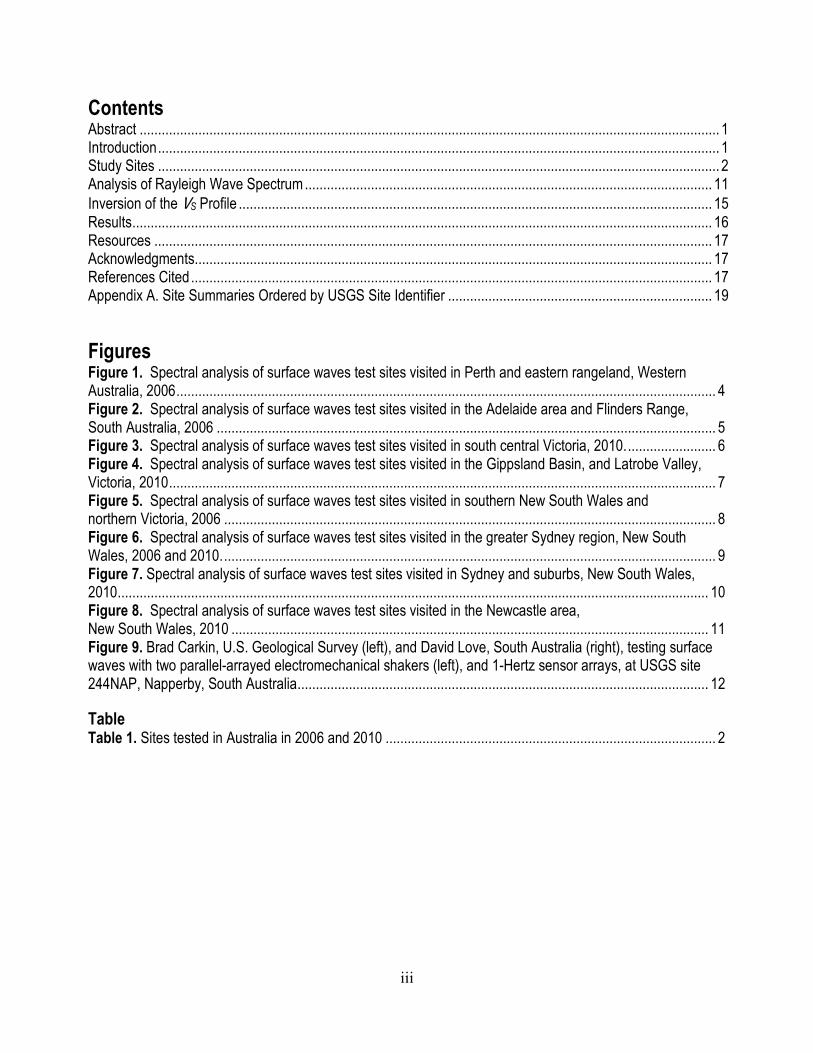
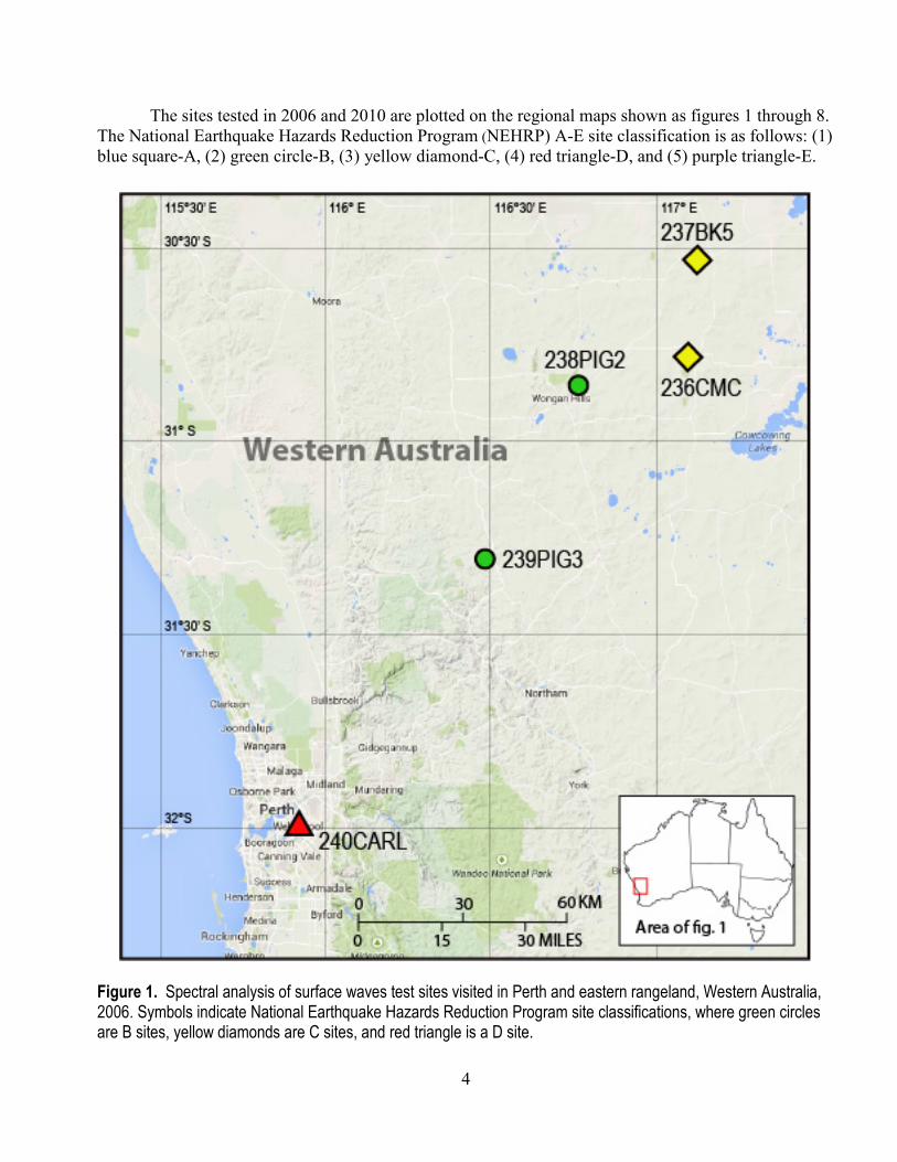
The sites tested in 2006 and 2010 are plotted on the regional maps shown as figures 1 through 8. The National Earthquake Hazards Reduction Program (NEHRP) A-E site classification is as follows: (1) blue square-A, (2) green circle-B, (3) yellow diamond-C, (4) red triangle-D, and (5) purple triangle-E.
Figure 1. Spectral analysis of surface waves test sites visited in Perth and eastern rangeland, Western Australia, 2006. Symbols indicate National Earthquake Hazards Reduction Program site classifications, where green circles are B sites, yellow diamonds are C sites, and red triangle is a D site.
5
Figure 2. Spectral analysis of surface waves test sites visited in the Adelaide area and Flinders Range, South Australia, 2006. Symbols indicate National Earthquake Hazards Reduction Program site classifications, where blue square is an A site, green circles are B sites, and red triangle is a D site.

6
Figure 3. Spectral analysis of surface waves test sites visited in south central Victoria, 2010. Symbols indicate National Earthquake Hazards Reduction Program site classifications, where green circles are B sites, yellow diamond is a C site, and red triangle is a D site.

7
Figure 4. Spectral analysis of surface waves test sites visited in the Gippsland Basin, and Latrobe Valley, Victoria, 2010. Symbols indicate National Earthquake Hazards Reduction Program site classifications, where green circle is a B site, red triangles are D sites, and purple triangle is an E site.

8
Figure 5. Spectral analysis of surface waves test sites visited in southern New South Wales and northern Victoria, 2006. Symbols indicate National Earthquake Hazards Reduction Program site classifications, where yellow diamonds are C sites, and green circles are B sites.

9
Figure 6. Spectral analysis of surface waves test sites visited in the greater Sydney region, New South Wales, 2006 and 2010. Symbols indicate National Earthquake Hazards Reduction Program site classifications, where green circles are B sites, and yellow diamonds are C sites.
10
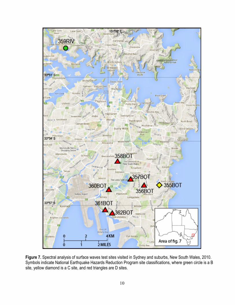
Figure 7. Spectral analysis of surface waves test sites visited in Sydney and suburbs, New South Wales, 2010. Symbols indicate National Earthquake Hazards Reduction Program site classifications, where green circle is a B site, yellow diamond is a C site, and red triangles are D sites.
11
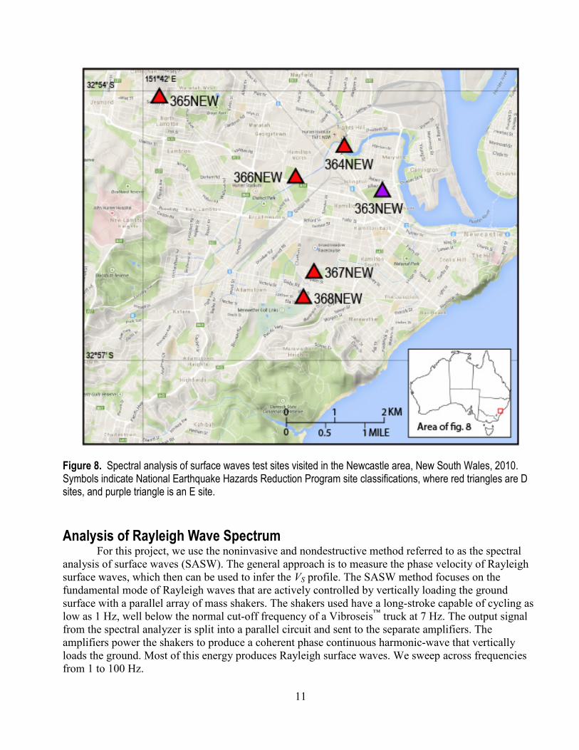
Figure 8. Spectral analysis of surface waves test sites visited in the Newcastle area, New South Wales, 2010. Symbols indicate National Earthquake Hazards Reduction Program site classifications, where red triangles are D sites, and purple triangle is an E site.
Analysis of Rayleigh Wave Spectrum
For this project, we use the noninvasive and nondestructive method referred to as the spectral analysis of surface waves (SASW). The general approach is to measure the phase velocity of Rayleigh surface waves, which then can be used to infer the VS profile. The SASW method focuses on the fundamental mode of Rayleigh waves that are actively controlled by vertically loading the ground surface with a parallel array of mass shakers. The shakers used have a long-stroke capable of cycling as low as 1 Hz, well below the normal cut-off frequency of a Vibroseis™ truck at 7 Hz. The output signal from the spectral analyzer is split into a parallel circuit and sent to the separate amplifiers. The amplifiers power the shakers to produce a coherent phase continuous harmonic-wave that vertically loads the ground. Most of this energy produces Rayleigh surface waves. We sweep across frequencies from 1 to 100 Hz.
12
Active-source surface wave analysis testing typically profiles the upper tens of meters of the ground using drop weights or harmonic sources. The upper 30 m is needed to compute the widely used site parameter VS30, defined as 30 m divided by the shear-wave travel time to 30 m depth. Deeper shear-wave profiles require lower frequencies and longer wavelengths that normally can not be collected unless a large drop weight (such as massive construction machinery) is used. For example, Kayen and others (2004) profiled the shear-wave structure of both sides of the Denali Fault using a 49-ton Caterpillar D9N™ bulldozer as an active source. Drop weights and heavy track-mounted machinery are useful tools for generating surface waves where the physical ground and landowners will support their presence. The two major drawbacks to this approach are that (1) these devices tend to be damaging to the ground surface, and (2) many sites of scientific importance are not easily accessible with such equipment.
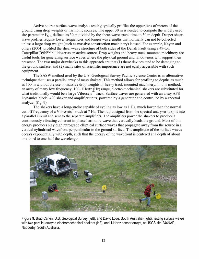
The SASW method used by the U.S. Geological Survey Pacific Science Center is an alternative technique that uses a parallel array of mass shakers. This method allows for profiling to depths as much as 100 m without the use of massive drop weights or heavy track-mounted machinery. In this method, an array of many low frequency, 100–1Hertz (Hz) range, electro-mechanical shakers are substituted for what traditionally would be a large Vibroseis™ truck. Surface waves are generated with an array APS Dynamics Model 400 shaker and amplifier units, powered by a generator and controlled by a spectral analyzer (fig. 9).
The shakers have a long-stroke capable of cycling as low as 1 Hz, much lower than the normal cut-off frequency of a Vibroseis™ truck at 7 Hz. The output signal from the spectral analyzer is split into a parallel circuit and sent to the separate amplifiers. The amplifiers power the shakers to produce a continuously vibrating coherent in-phase harmonic-wave that vertically loads the ground. Most of this energy produces Rayleigh retrograde elliptical surface waves that propagate away from the source in a vertical cylindrical wavefront perpendicular to the ground surface. The amplitude of the surface waves decays exponentially with depth, such that the energy of the wavefront is centered at a depth of about one-third to one-half the wavelength.
Figure 9. Brad Carkin, U.S. Geological Survey (left), and David Love, South Australia (right), testing surface waves with two parallel-arrayed electromechanical shakers (left), and 1-Hertz sensor arrays, at USGS site 244NAP, Napperby, South Australia.
13
Frequency domain analyses are made on two or more signals received by sensors placed in the field in the linear array some distance from the source. First, all channels of time domain data are transformed into their equivalent linear spectrum in the frequency domain using a Fourier transform. One of the sensor signals (typically from the sensor closest to the source) is used for a reference input signal, and the other sensor signals are used to compute the linear spectrums of the output. The separation of the reference seismometer and output seismometer (ds–dref) radially from the source later is used to compute the wave velocity. The cross power spectrum Gxy(ω) is determined by multiplying the complex conjugate of the linear spectrum of the input signal Sx
*(ω), and the real portion of the linear spectrum of the output signal Sy(ω). The cross power spectrum is defined as
Gxy(ω) = Sx*(ω) × Sy(ω) (1)
The autopower spectrum, a measure of the energy at each frequency of the sweep, can be used to determine the strength of individual frequencies, and is equal to the linear spectrum of a given sensor times its complex conjugate pair:
Gxx(ω) = Sx(ω) × Sx*(ω), and (2)
Gyy(ω) = Sy(ω) × Sy*(ω). (3)
A cross power spectrum can be represented by its real and imaginary components to determine phase θ, and magnitude m. The phase θ is the relative lag between the signals at each frequency, and the magnitude is a measure of the power between the two signals at each frequency. Because the phases are relative, they can be stacked to enhance signal-to-noise ratio of the phase lag at each frequency.
The phase of the cross power spectrum is computed as the inverse tangent of the ratio of the imaginary and real portions of the cross power spectrum:
𝜃𝑥𝑥(𝜔) = 𝑡𝑡𝑡−1 𝐼𝐼�𝐺𝑥𝑥(𝜔)�𝑅𝑅�𝐺𝑥𝑥(𝜔)�
(4)
The travel time t(ƒ) of one cycle of a wave of frequency (ƒ) is computed as,
t(f) = θ(ω)/ω (5)
and the wavelength, λ, at each frequency is
λ(θ) = (ds–dref)/ θ(ƒ) (6)
The Rayleigh wave velocity, Vr, is computed as
Vr(f) = (ds–dref)/t(ƒ)
= ƒ(ds–dref) 360°/θ (degrees)
= ƒ(ds–dref) 2π/θ(ƒ) (radians)
= ƒλ(ƒ) (7)

14
The SASW procedure maps the change in θ across the frequency spectrum, and merges these phase lags with the sensor array geometry to measure velocity. With the shaker source, the discrete frequencies typically are cycled in a swept (stepped)-sine fashion across a range of low frequencies (1–200 Hz). Rayleigh-wave phase velocity then is mapped in frequency or wavelength space. This velocity map or profile is referred to as a dispersion curve and characterizes changes in the frequency-dependent Rayleigh wave velocity. The evaluation of velocities is constrained to the wavelength zone where λ(f)/3 < (ds–dref) < 2 λ(f) for typical data and λ(f)/3 < (ds–dref) < 3 λ(f) for excellent data, corresponding to phase lags of 180°–1080° (typical data) and 120°–1080° (excellent data). At longer and shorter wavelengths, the data become unreliable for computing velocities.
As the useable wavelengths are constrained by the seismometer separation, the array is expanded to capture Rayleigh wave dispersion representative of a specific range of wavelengths. The near surface is characterized by short wavelengths and high frequencies, whereas the deeper part of the profile is characterized by long wavelengths and low frequencies. Each wavelength range requires a separate independent test that is merged together with other wavelength ranges to determine an average dispersion curve for the site.
At the largest seismometer separations, the increasing area of the wavefront causes the wave amplitude to diminish because of geometric damping, and the overall quality of the data diminishes. Two measures of data quality are used to evaluate the field measurements in the frequency domain. Coherence, γ2(ω), is a normalized real function with values between 0 and 1 corresponding to the ratio of the power of the cross power spectrum, Gyx(ω) • Gyx
*(ω), to the autopower spectrum of the outboard seismometer, Gxx(ω) • Gyy(ω). Values close to 1 indicate high correlation between the reference and outboard seismometers across narrow frequency bands. This is a useful data quality parameter for hammer impact data.
𝛾𝑥𝑥2 (𝜔) = 𝐺𝑥𝑥(𝜔)•𝐺𝑥𝑥∗ (𝜔)𝐺𝑥𝑥(𝜔)•𝐺𝑥𝑥(ω)
(8)
For swept sine data where discrete frequencies are used to compute phase rather than narrow frequency bands, the frequency response function, FRF, is a complex measure of the data quality of the output (outboard) seismometer, and is sometimes referred to as the Transfer Function:
FRF(ω) = 𝐺𝑥𝑥(𝜔)
𝐺𝑥𝑥(𝜔) (9)
where x is the input (reference) signal, and y is the response (output) signal.
The Frequency Response Function is a two-sided complex parameter. To convert to the frequency response gain (magnitude) that is used to evaluate the amplitude of the output response to the input stimulus, a rectangular-to-polar coordinate conversion is used.

15
Inversion of the VS Profile The relation between Rayleigh wave (VR), shear wave (VS) and compression wave (VP) velocities
can be formulated through Navier's equations for dynamic equilibrium. At the ground surface in the case of plane strain, the following characteristic equation is:
𝑉𝑟𝑉𝑠
6- 8 𝑉𝑟
𝑉𝑠
4+(24-16� 1−2𝜈
2(1−𝜈)�) 𝑉𝑟
𝑉𝑠
2+ 16 �� 1−2𝜈
2(1−𝜈)� − 1� = 0 (10)
where ν is the Poisson ratio and
𝑉𝑆𝑉𝑃
= 𝛾 = �� 1−2𝜈2(1−𝜈)
� (11)
For reasonable values of Poisson Ratio for earth materials, between 0.20 and 0.49, Viktorov (1967) shows that the shear wave velocity ranges from 105 to 115 percent of the measured Rayleigh wave velocity
𝑉𝑅𝑉𝑆
= 𝐾 = 0.87+1.12𝜈1+𝜈
(12)
such that across the range 0.2<ν<0.49, the range of K is 0.87<K<0.96. The inversion method seeks to infer an acceptable best-fit model of seismic shear wave velocity,
VS, of the ground given the measured dispersive characteristics of Rayleigh waves observed in the frequency domain, and the estimated profile of Poisson ratio and material density. The inversion attempts to build a model from observations, as compared to the normal prediction of behavior based on a model. If the inversion model is simple and linear, it will result in a unique and stable solution. The French mathematician Hadamard defined mathematical problems that have solutions, are unique, and are stable as “well-posed” (Zhdanov, 2002). By contrast, surface wave inversion is an “ill-posed” inverse problem, as solutions are not unique, the solutions may become unstable, and multiple shear wave velocity profiles can result in approximately the same dispersion curve (Zhdanov, 2002).
The dispersive characteristic of Rayleigh wave propagation allows us to infer the VS at depth based on measurements at the free surface. The forward model computes the Rayleigh wave phase velocity (VR) from laterally constant layers of an infinite half space. For each of these layers, the shear modulus, Poisson ratio, density, and thickness are unknown. Displacements for a vertically acting harmonic point load can be computed as follows in the far field if body wave components are disregarded:
𝑢𝛽(𝑟, 𝑧,𝜔) = 𝐹𝑧 ∙ 𝐺𝛽 ∙ (𝑟, 𝑧,𝜔) ∙ 𝑒𝑖[𝜔𝜔−𝜓𝛽(𝑟,𝑧,𝜔)] (13)
where β stands for the generic component either vertical or radial,
Gβ(r,z,ω) is the Rayleigh geometrical spreading function, and Ψβ(r,z,ω) is the composite phase function (Lai and Rix, 1998; Foti, 2000).

16
Regularization methods have been developed for solving the ill-posed problem if inversion of stiffness from surface wave dispersion data. The Levenberg-Marquardt method, also referred to as damped least squares, is one example of a regularization method. These and other techniques, such as artificial neural networks and genetic algorithms, are discussed by Santamarina and Fratta (1998). One cost of these stochastic methods is that they often require many more iterations, and so they are much more computationally intensive.
The parameters of the forward problem can be selected so that the difference between the observational dispersion data and the output of the forward problem are minimized. Such a constraint is insufficient for ill-posed problems because many solutions can fit the data equally well, and some of these solutions will be physically unrealistic. The most common approach is to constrain the inversion solution space by selecting the smoothest solution from a suite of solutions that all indicate a sufficient goodness-of-fit to the observed data, as indicated by a root mean square error minimum
An empirical approach serves as a counterpoint to the forward inversion methods with the forward model method used in this report. Pelekis and Athanosopoulos (2011) advanced the work of Satoh and others (1991) in a technique termed the Simplified Inversion Method that computes the shear wave velocity profile as a function of the incremental slope of the Rayleigh wave dispersion curve where:
𝑉𝑆𝑆,𝑆𝑛𝑟𝐼𝑛𝑛 𝑑𝑖𝑑𝑑𝑅𝑟𝑑𝑖𝑛𝑆 = 1.1 ∙ 𝑉�𝑅𝑅𝐷𝑅−𝑉�𝑅𝑅−1𝐷𝑅−1
𝐷𝑅−𝐷𝑅−1 (14)
𝑉𝑆𝑆,𝑖𝑆𝑖𝑅𝑟𝜔𝑅𝑑 𝑑𝑖𝑑𝑑𝑅𝑟𝑑𝑖𝑛𝑆 = 1.1 ∙ 𝐷𝑅−𝐷𝑅−1𝐷𝑅 𝑉�𝑅𝑅⁄ − 𝐷𝑅−1 𝑉�𝑅𝑅−1⁄ (15)
The dispersion curve VR plotted against λR is converted into an apparent velocity (𝑉�R) and depth (z) by converting λR to an estimated depth of 𝑧𝑅𝑒 = 𝑡𝑅 ∙ 𝜆𝑅 ≈ 0.635𝜆𝑅 . The parameter aR is a penetration depth coefficient optimized to achieve a minimum weighted average difference between the simplified velocity profile and that computed through the more advanced forward inversion of Pelekis and Athansopoulos (2011). The apparent phase velocity, 𝑉𝑅���, is approximated as the velocity at each segment node (layer interface) of a multi-linear curve fit to the dispersion curve. A positive slope of a segment indicates normal dispersion; a negative slope indicates inverted dispersion. The value of VS for each individual layer is calculated using equations 14 and 15 for the cases of normal dispersion or inverted dispersion, respectively. The approach of Pelekis and Athansopoulos (2011) improves on method of Satoh and others (1991), notably by optimizing the penetration depth coefficient, aR.
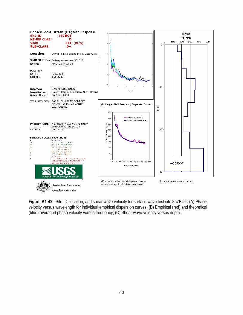
Results Two profile solutions are provided at each site (Forward Inversion and Simplified Inversion
Method model). We varied the assumptions about the layer thicknesses and the threshold root mean square error that determines if the inversion has converged to best characterize the site. Whether or not the more complex model is warranted by the fit of the theoretical dispersion curve to the empirical dispersion curve is a subjective decision.
Profile results are summarized in table 1, including the following information provided: SASW site ID, site location, date of data collection, site latitude and longitude, and site parameter VS30.
Plots of the two model profiles and the empirical dispersion curve and theoretical dispersion curves for each site are included in appendix A. Site photographs and a vicinity map for each site also are included in appendix A. Where possible, we have indicated the location of the strong motion station in the site photographs and vicinity maps to assess the distance between the SASW survey and the strong motion station.

17
Resources We have used the SWAMI Fortran routines that are freely available at
http://geosystems.ce.gatech.edu/soil_dynamics/research/surfacewavesanalysis/ (distributed under the terms of the GNU General Public License).
Acknowledgments This work is supported through Project annex AS-02.0400 under the memorandum of
understanding on scientific and technical cooperation in the geosciences between the United States (U.S. Geological Survey, Department of the Interior) and Australia (Geoscience Australia, Department of Industry, Tourism and Resources). We thank Andrew McPherson, Trevor Allen, Clive Collins and David Burbidge for their interest and support of this study. Owen McConnel , David Love, and Kirkland Kalder-Bull, with the governments of Western Australia, South Australia, and Victoria, respectively, were of great assistance to our data-collection efforts.
References Cited Foti, S., 2000, Multistation methods for geotechnical characterization using surface waves: Turin, Italy,
Politecnico di Torino, Ph.D. dissertation, 251 p. Kayen, R., Seed, R.B., Moss, R.E., Cetin, O., Tanaka, Y., and Tokimatsu, K., 2004, Global shear wave
velocity database for probabilistic assessment of the initiation of seismic-soil liquefaction: International conference on soil dynamics and earthquake engineering, 11th, Berkeley, California, January 7–9, 2004, p. 506–512.
Lai, C.G., and Rix, G. J., 1998, Simultaneous inversion of Rayleigh phase velocity and attenuation for near-surface site characterization: Georgia Institute of Technology, School of Civil and Environmental Engineering Report No. GIT-CEE/GEO-98-2, 258 p.
Pelekis, P.C., and Athanasopoulos, G.A., 2011, An overview of surface wave methods and a reliability study of a simplified inversion technique: Soil Dynamics and Earthquake Engineering, v. 31, no. 12, p. 1,654–1,668.
Santamarina, J.C., and Fratta, D., 1998, Introduction to discrete signals and inverse problems in civil engineering: American Society of Civil Engineers, 327 p.
Satoh, T., Poran, C.I., Yamagata, K., and Rondriquez, J.A., 1991, Soil profiling by spectral analysis of surface waves: International conference on recent advances in geotechnical earthquake engineering and soil dynamics, 2nd, 1991, v.2, p. 1,429–1,434.
Viktorov, I.A., 1967, Rayleigh and lamb waves—Physical theory and applications, New York, Plenum Press, 154 p.
Zhdanov, M.S., 2002, Geophysical inverse theory and regularization problems: Methods in Geochemistry and Geophysics, Elsevier, v. 36, 628 p.

18
This page left intentionally blank

19
Appendix A. Site Summaries Ordered by USGS Site Identifier
Figure A1-1. Surface wave test site 236CMC located 2.3 km SW of Cadoux, Western Australia (lat -30.79102, long 117.0963). Tested on June 10, 2006. (A) view towards the east from shakers; (B) view NE from seismometer and borehole toward the shakers behind vehicle; (C) view SW from shakers; (D) view to the west along seismometer array; (E) satellite view of the local site, red and white symbol is the location of the shakers, the yellow bar is the seismometer array; (F) site location in Western Australia.

20
Figure A1-2. Site ID, location, and shear wave velocity for surface wave test site 236CMC. (A) Phase velocity versus wavelength for individual empirical dispersion curves; (B) Phase velocity versus frequency for individual empirical dispersion curves; (C) Empirical (red) and theoretical (blue) averaged phase velocity versus frequency; (D) Shear wave velocity versus depth.

21
Figure A1-3. Surface wave test site 237BK5 located about 5 km west of Burakin, Western Australia (lat -30.5194, long 117.12187). Tested on June 11, 2006. (A) view looking eastward toward shakers; (B) view westward from shakers; (C) shakers at the east end of array; (D) landmark near the west end of seismometer array; (E) satellite view of the local site, red and white symbol is the location of the shakers, the yellow bar is the seismometer array; (F) site location in Western Australia.

22
Figure A1-4. Site ID, location and shear wave velocity for surface wave test site 237BK5. (A) Phase velocity versus wavelength for individual empirical dispersion curves; (B) Phase velocity versus frequency for individual empirical dispersion curves; (C) Empirical (red) and theoretical (blue) averaged phase velocity versus frequency; (D) Shear wave velocity versus depth.

23
Figure A1-5. Surface wave test site 238PIG2 located 8.5 km NE of Wongan Hills, Western Australia (lat -30.84753, long 116.79184). Tested on June 11, 2006. (A) view looking southwards to the shakers; (B) view north to the seismometer array; (C) view towards the NE from shakers; (D) view of local bedrock exposure near the seismometer array, about 100 m to the east; (E) satellite view of the local site, red and white symbol is the location of the shakers, the yellow bar is the seismometer array; (F) site location in Western Australia.

24
Figure A1-6. Site ID, location, and shear wave velocity for surface wave test site 238PIG2. (A) Phase velocity versus wavelength for individual empirical dispersion curves; (B) Phase velocity versus frequency for individual empirical dispersion curves; (C) Empirical (red) and theoretical (blue) averaged phase velocity versus frequency; (D) Shear wave velocity versus depth.

25
Figure A1-7. Surface wave test site 239PIG3 located 5.4 km SW of Bolgart, Western Australia (lat -31.31517, long 116.48366). Tested on June 12, 2006. (A) view looking southeastwards from the shakers; (B) view looking NW toward shakers; (C) view to the east at the shakers; (D) seismometer, battery and solar panel on rock knob, behind the vehicle in B; (E) satellite view of the local site, red and white symbol is the location of the shakers, the yellow bar is the seismometer array; (F) site location in Western Australia.
26
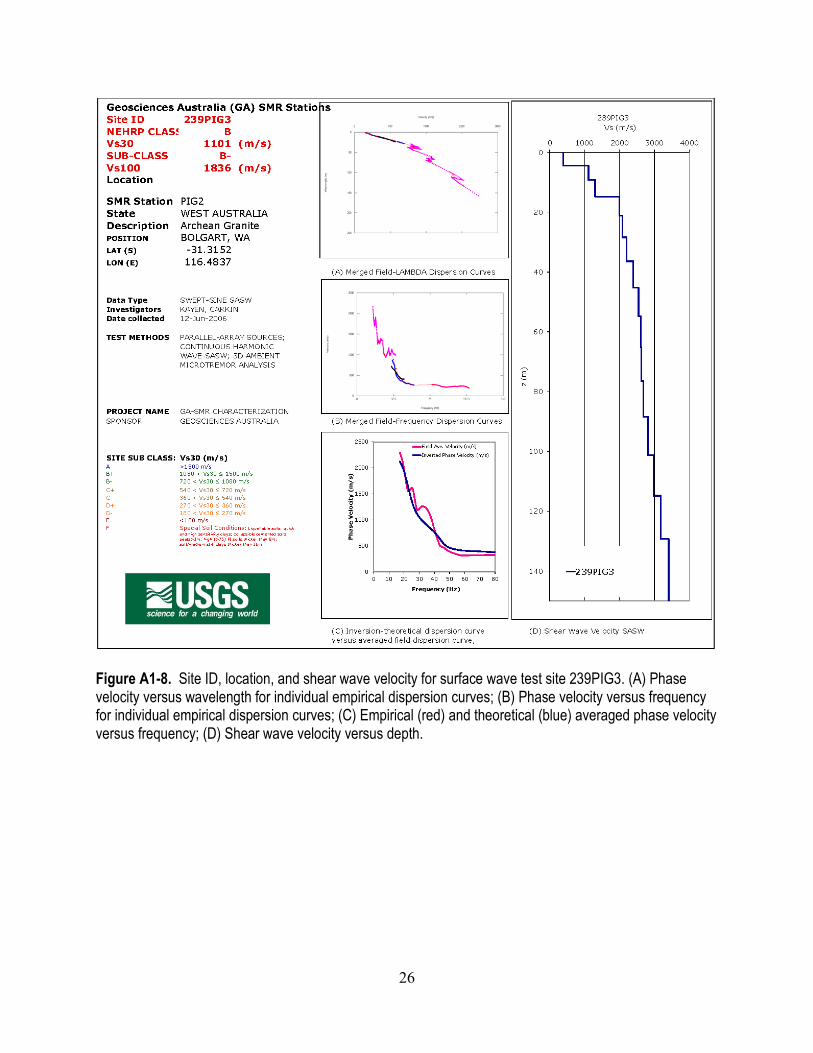
Figure A1-8. Site ID, location, and shear wave velocity for surface wave test site 239PIG3. (A) Phase velocity versus wavelength for individual empirical dispersion curves; (B) Phase velocity versus frequency for individual empirical dispersion curves; (C) Empirical (red) and theoretical (blue) averaged phase velocity versus frequency; (D) Shear wave velocity versus depth.

27
Figure A1-9. Surface wave test site 240CAR located in Carlisle, suburb of Perth, Western Australia (lat -31.983031, long 115.926921). Tested on June 13, 2006. (A) view looking NW towards the shaker location; (B) view looking SE along seismometer array; (C) SE end of the seismometer array looking NW; (D) entrance to facility on Harris Street; (E) satellite view of the local site, red and white symbol is the location of the shakers, the yellow bar is the seismometer array; (F) site location in Western Australia.
28
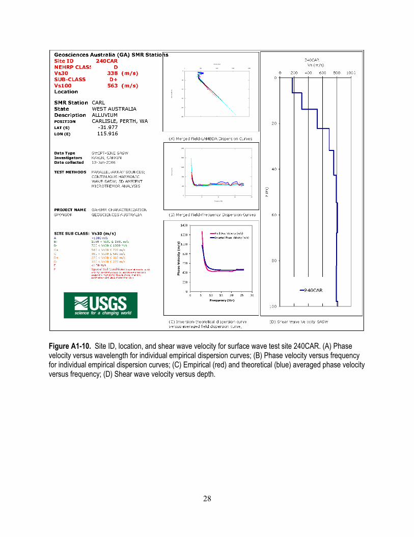
Figure A1-10. Site ID, location, and shear wave velocity for surface wave test site 240CAR. (A) Phase velocity versus wavelength for individual empirical dispersion curves; (B) Phase velocity versus frequency for individual empirical dispersion curves; (C) Empirical (red) and theoretical (blue) averaged phase velocity versus frequency; (D) Shear wave velocity versus depth.

29
Figure A1-11. Surface wave test site 241SDN located 8 km NE of Sedan, South Australia (lat -34.5093, long 139.3374). Tested on June 15, 2006. (A) view looking towards the northeast from shakers; (B) view SW toward the shakers; (C) view looking east at a seismometer on array; (D) seismometer shelter and solar panel located at the red arrow in E; (E) satellite view of the local site, red and white symbol is the location of the shakers, the yellow bar is the seismometer array; (F) site location in South Australia.

30
Figure A1-12. Site ID, location, and shear wave velocity for surface wave test site 241SDN. (A) Phase velocity versus wavelength for individual empirical dispersion curves; (B) Phase velocity versus frequency for individual empirical dispersion curves; (C) Empirical (red) and theoretical (blue) averaged phase velocity versus frequency; (D) Shear wave velocity versus depth.

31
Figure A1-13. Surface wave test site 242FR14 located 4.2 km NW of Spalding, South Australia (lat -33.4709, long 138.5757). Tested on June 16, 2006. (A) view looking towards the SW down ridge line from shakers; (B) view looking SW down ridge line; (C) view SW from shakers, 2 m seismometer separation; (D) view looking NE uphill toward shakers; (E) satellite view of the local site, red and white symbol is the location of the shakers, the yellow bar is the seismometer array; (F) site location in South Australia.
32
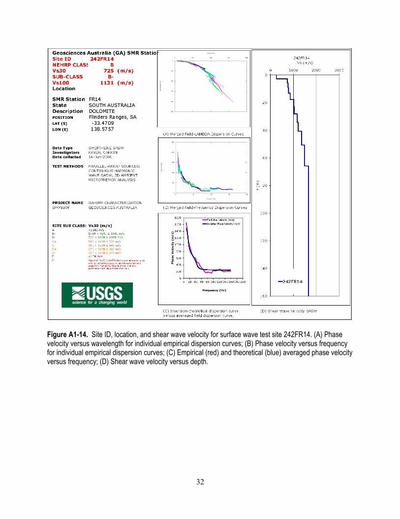
Figure A1-14. Site ID, location, and shear wave velocity for surface wave test site 242FR14. (A) Phase velocity versus wavelength for individual empirical dispersion curves; (B) Phase velocity versus frequency for individual empirical dispersion curves; (C) Empirical (red) and theoretical (blue) averaged phase velocity versus frequency; (D) Shear wave velocity versus depth.

33
Figure A1-15. Surface wave test site 243FR13 located about 9 km NW of Jamestown, South Australia (lat -33.1249, long 138.5683). Tested on June 16, 2006. (A) view looking westward from the shakers; (B) view looking SW above test site; (C) view NE from the shakers; (D) view to the west along seismometer array; (E) satellite view of the local site, red and white symbol is the location of the shakers, the yellow bar is the seismometer array; F) site location in South Australia.

34
Figure A1-16. Site ID, location, and shear wave velocity for surface wave test site 243FR13. (A) Phase velocity versus wavelength for individual empirical dispersion curves; (B) Phase velocity versus frequency for individual empirical dispersion curves; (C) Empirical (red) and theoretical (blue) averaged phase velocity versus frequency; (D) Shear wave velocity versus depth.

35
Figure A1-17. Surface wave test site 244NAP located 4 km SE of Napperby, South Australia (lat -33.184, long 138.145). Tested on June 17, 2006. (A) view looking towards the west from shakers; (B) view to the SE up the gulley along seismometer array; (C) view northward from shakers; (D) seismometer shelter located at the red arrow in E; (E) satellite view of the local site, red and white symbol is the location of the shakers, the yellow bar is the seismometer array; (F) site location in South Australia.
36
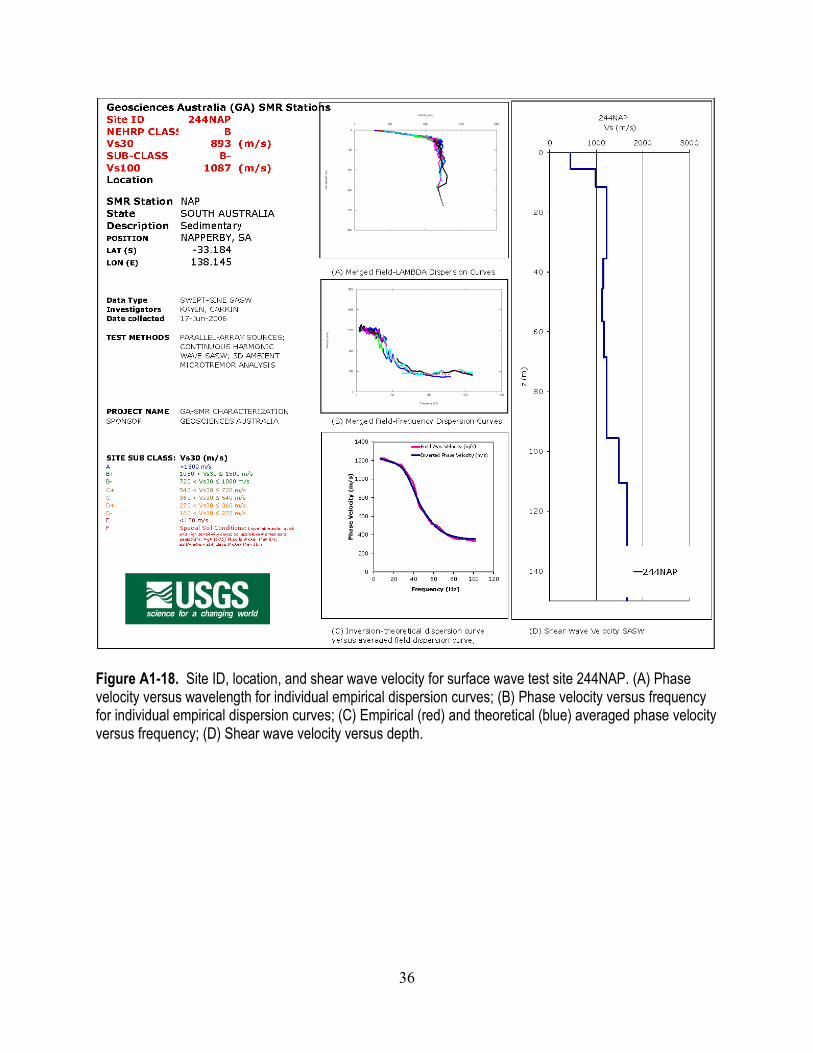
Figure A1-18. Site ID, location, and shear wave velocity for surface wave test site 244NAP. (A) Phase velocity versus wavelength for individual empirical dispersion curves; (B) Phase velocity versus frequency for individual empirical dispersion curves; (C) Empirical (red) and theoretical (blue) averaged phase velocity versus frequency; (D) Shear wave velocity versus depth.
37
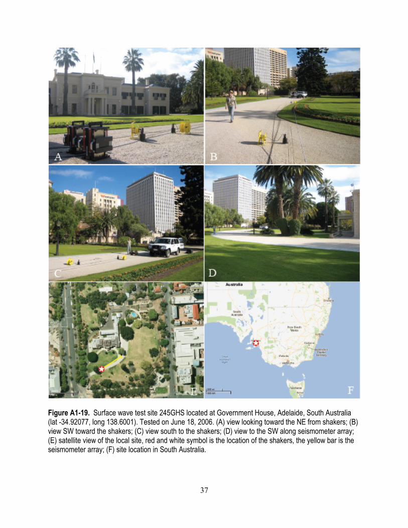
Figure A1-19. Surface wave test site 245GHS located at Government House, Adelaide, South Australia (lat -34.92077, long 138.6001). Tested on June 18, 2006. (A) view looking toward the NE from shakers; (B) view SW toward the shakers; (C) view south to the shakers; (D) view to the SW along seismometer array; (E) satellite view of the local site, red and white symbol is the location of the shakers, the yellow bar is the seismometer array; (F) site location in South Australia.

38
Figure A1-20. Site ID, location, and shear wave velocity for surface wave test site 245GHS. (A) Phase velocity versus wavelength for individual empirical dispersion curves; (B) Phase velocity versus frequency for individual empirical dispersion curves; (C) Empirical (red) and theoretical (blue) averaged phase velocity versus frequency; (D) Shear wave velocity versus depth.

39
Figure A1-21. Surface wave test site 246DTM located on ridge top about 70 km SW of Wodonga, Victoria (lat -36.5293, long 147.469). Tested on June 21, 2006. (A) photo view towards the SE at the shakers; (B) view Sw from the shakers; (C) view SE along seismometer array; (D) seismometer shelter on south-facing side of ridge; (E) satellite view of the local site, red and white symbol is the location of the shakers, the yellow bar is the seismometer array; (F) site location in Victoria.

40
Figure A1-22. Site ID, location, and shear wave velocity for surface wave test site 246DTM. (A) Phase velocity versus wavelength for individual empirical dispersion curves; (B) Phase velocity versus frequency for individual empirical dispersion curves; (C) Empirical (red) and theoretical (blue) averaged phase velocity versus frequency; (D) Shear wave velocity versus depth.

41
Figure A1-23. Surface wave test site 247LGT located about 88 km SE of Wodonga, Victoria (lat -36.7633, long 147.464). Tested on June 21, 2006. (A) view of shakers and seismometers; (B) view NW or SE along seismometer array; (C) view of shakers and seismometers, 2 m spacing; (D) seismometer shelter; (E) satellite view of the local site, red and white symbol is the location of the shakers based on GPS, trend of the seismometer array is uncertain on irregular forest road; (F) site location in Victoria.

42
Figure A1-24. Site ID, location, and shear wave velocity for surface wave test site 247LGT. (A) Phase velocity versus wavelength for individual empirical dispersion curves; (B) Phase velocity versus frequency for individual empirical dispersion curves; (C) Empirical (red) and theoretical (blue) averaged phase velocity versus frequency; (D) Shear wave velocity versus depth.
43
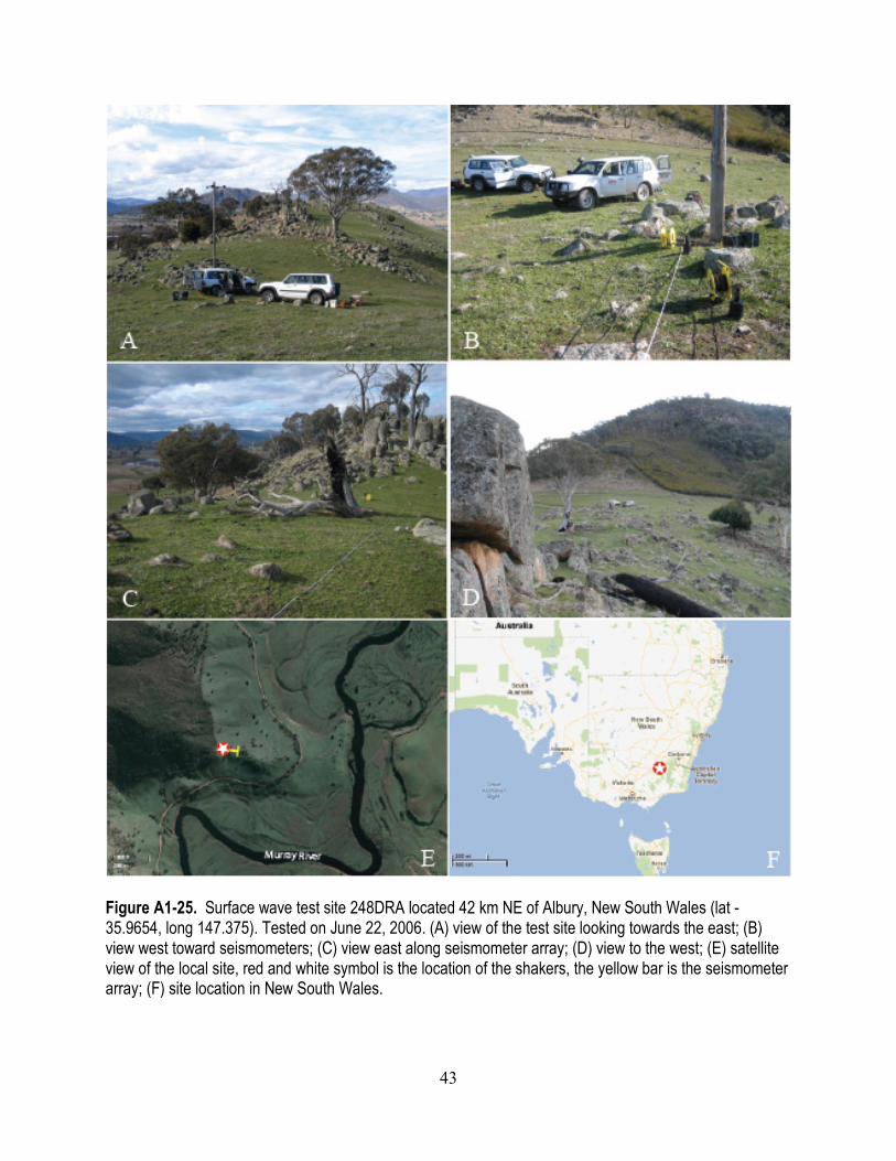
Figure A1-25. Surface wave test site 248DRA located 42 km NE of Albury, New South Wales (lat -35.9654, long 147.375). Tested on June 22, 2006. (A) view of the test site looking towards the east; (B) view west toward seismometers; (C) view east along seismometer array; (D) view to the west; (E) satellite view of the local site, red and white symbol is the location of the shakers, the yellow bar is the seismometer array; (F) site location in New South Wales.

44
Figure A1-26. Site ID, location, and shear wave velocity for surface wave test site 248DRA. (A) Phase velocity versus wavelength for individual empirical dispersion curves; (B) Phase velocity versus frequency for individual empirical dispersion curves; (C) Empirical (red) and theoretical (blue) averaged phase velocity versus frequency; (D) Shear wave velocity versus depth.
45
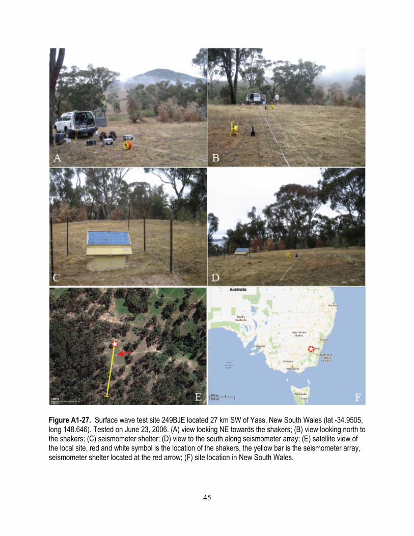
Figure A1-27. Surface wave test site 249BJE located 27 km SW of Yass, New South Wales (lat -34.9505, long 148.646). Tested on June 23, 2006. (A) view looking NE towards the shakers; (B) view looking north to the shakers; (C) seismometer shelter; (D) view to the south along seismometer array; (E) satellite view of the local site, red and white symbol is the location of the shakers, the yellow bar is the seismometer array, seismometer shelter located at the red arrow; (F) site location in New South Wales.

46
Figure A1-28. Site ID, location, and shear wave velocity for surface wave test site 249BJE. (A) Phase velocity versus wavelength for individual empirical dispersion curves; (B) Phase velocity versus frequency for individual empirical dispersion curves; (C) Empirical (red) and theoretical (blue) averaged phase velocity versus frequency; (D) Shear wave velocity versus depth.
47
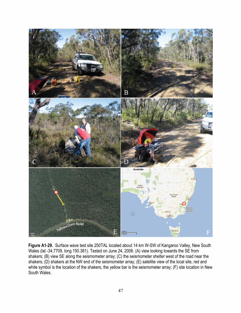
Figure A1-29. Surface wave test site 250TAL located about 14 km W-SW of Kangaroo Valley, New South Wales (lat -34.7709, long 150.381). Tested on June 24, 2006. (A) view looking towards the SE from shakers; (B) view SE along the seismometer array; (C) the seismometer shelter west of the road near the shakers; (D) shakers at the NW end of the seismometer array; (E) satellite view of the local site, red and white symbol is the location of the shakers, the yellow bar is the seismometer array; (F) site location in New South Wales.

48
Figure A1-30. Site ID, location, and shear wave velocity for surface wave test site 250TAL. (A) Phase velocity versus wavelength for individual empirical dispersion curves; (B) Phase velocity versus frequency for individual empirical dispersion curves; (C) Empirical (red) and theoretical (blue) averaged phase velocity versus frequency; (D) Shear wave velocity versus depth.
49
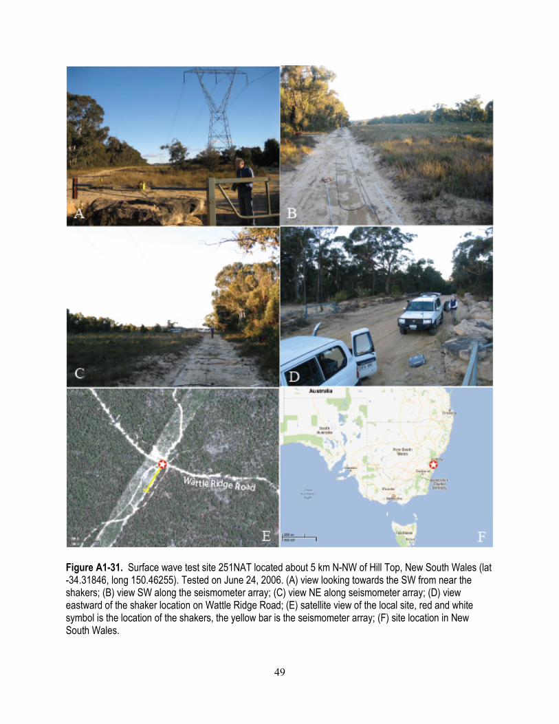
Figure A1-31. Surface wave test site 251NAT located about 5 km N-NW of Hill Top, New South Wales (lat -34.31846, long 150.46255). Tested on June 24, 2006. (A) view looking towards the SW from near the shakers; (B) view SW along the seismometer array; (C) view NE along seismometer array; (D) view eastward of the shaker location on Wattle Ridge Road; (E) satellite view of the local site, red and white symbol is the location of the shakers, the yellow bar is the seismometer array; (F) site location in New South Wales.

50
Figure A1-32. Site ID, location, and shear wave velocity for surface wave test site 251NAT. (A) Phase velocity versus wavelength for individual empirical dispersion curves; (B) Phase velocity versus frequency for individual empirical dispersion curves; (C) Empirical (red) and theoretical (blue) averaged phase velocity versus frequency; (D) Shear wave velocity versus depth.
51
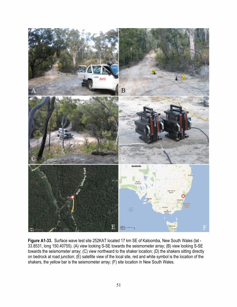
Figure A1-33. Surface wave test site 252KAT located 17 km SE of Katoomba, New South Wales (lat -33.8531, long 150.40755). (A) view looking S-SE towards the seismometer array; (B) view looking S-SE towards the seismometer array; (C) view northward to the shaker location; (D) the shakers sitting directly on bedrock at road junction; (E) satellite view of the local site, red and white symbol is the location of the shakers, the yellow bar is the seismometer array; (F) site location in New South Wales.

52
Figure A1-34. Site ID, location, and shear wave velocity for surface wave test site 252KAT. (A) Phase velocity versus wavelength for individual empirical dispersion curves; (B) Phase velocity versus frequency for individual empirical dispersion curves; (C) Empirical (red) and theoretical (blue) averaged phase velocity versus frequency; (D) Shear wave velocity versus depth.

53
Figure A1-35. Surface wave test site 253LUC located at the High Flux Australian Reactor site, Lucas Heights, New South Wales (lat -34.05181, long 150.97958). Tested on June 27, 2006. (A) satellite view of the reactor and test site, red and white symbol is the location of the shakers, the yellow bar is the seismometer array; (B) wider satellite view of reactor site and shaker location; (C) site location in New South Wales.

54
Figure A1-36. Site ID, location, and shear wave velocity for surface wave test site 253LUC. (A) Phase velocity versus wavelength for individual empirical dispersion curves; (B) Phase velocity versus frequency for individual empirical dispersion curves; (C) Empirical (red) and theoretical (blue) averaged phase velocity versus frequency; (D) Shear wave velocity versus depth.

55
Figure A1-37. Surface wave test site 355BOT, Latham Park, eastern suburbs, Sydney, New South Wales (lat -33.93479, long 151.25119). Botany microtremor site 305006, tested on April 15, 2010. (A) view southward to the seismometer array from the shakers; (B) view northward to the shakers; (C) view north to the seismometers and shakers; (D) view west at the shakers; (E) satellite view of the local site, red and white symbol is the location of the shakers, the yellow bar is the seismometer array; (F) site location in New South Wales.

56
Figure A1-38. Site ID, location, and shear wave velocity for surface wave test site 355BOT. (A) Phase velocity versus wavelength for individual empirical dispersion curves; (B) Empirical (red) and theoretical (blue) averaged phase velocity versus frequency; (C) Shear wave velocity versus depth.

57
Figure A1-39. Surface wave test site 356BOT, Snape Park, Maroubra, eastern suburbs, Sydney (lat -33.93572, long 151.2332). Botany microtremor site 301016, tested on April 16, 2010. (A) view westward from the shakers; (B) view east at the seismometers and shakers; (C) view NE from the shakers into playing field; (D) satellite view of the local site, red and white symbol is the location of the shakers, the yellow bar is the seismometer array; (E) site location in New South Wales.

58
Figure A1-40. Site ID, location, and shear wave velocity for surface wave test site 356BOT. (A) Phase velocity versus wavelength for individual empirical dispersion curves; (B) Empirical (red) and theoretical (blue) averaged phase velocity versus frequency; (C) Shear wave velocity versus depth.
59
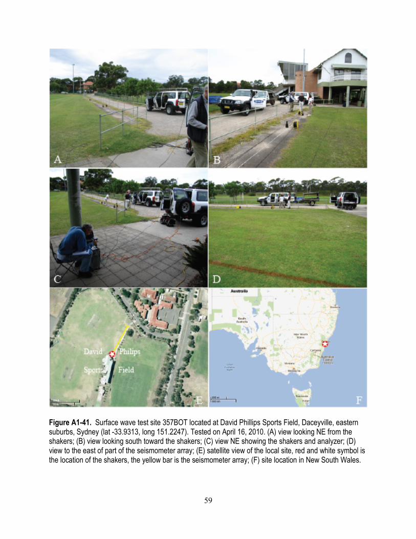
Figure A1-41. Surface wave test site 357BOT located at David Phillips Sports Field, Daceyville, eastern suburbs, Sydney (lat -33.9313, long 151.2247). Tested on April 16, 2010. (A) view looking NE from the shakers; (B) view looking south toward the shakers; (C) view NE showing the shakers and analyzer; (D) view to the east of part of the seismometer array; (E) satellite view of the local site, red and white symbol is the location of the shakers, the yellow bar is the seismometer array; (F) site location in New South Wales.
60
Figure A1-42. Site ID, location, and shear wave velocity for surface wave test site 357BOT. (A) Phase velocity versus wavelength for individual empirical dispersion curves; (B) Empirical (red) and theoretical (blue) averaged phase velocity versus frequency; (C) Shear wave velocity versus depth.

61
Figure A1-43. Surface wave test site 358BOT located in Rosebery, southeastern suburbs, Sydney, New South Wales (lat -33.91608, long 151.208491). Botany microtremor site 301035, tested on April 16, 2010. (A) view looking east from shakers along Kimbereley Grove; (B) view west along seismometer array; (C) view of the shakers looking NE; (D) view to the west to the shakers; (E) satellite view of the local site, red and white symbol is the location of the shakers, the yellow bar is the seismometer array; (F) site location in New South Wales.
62
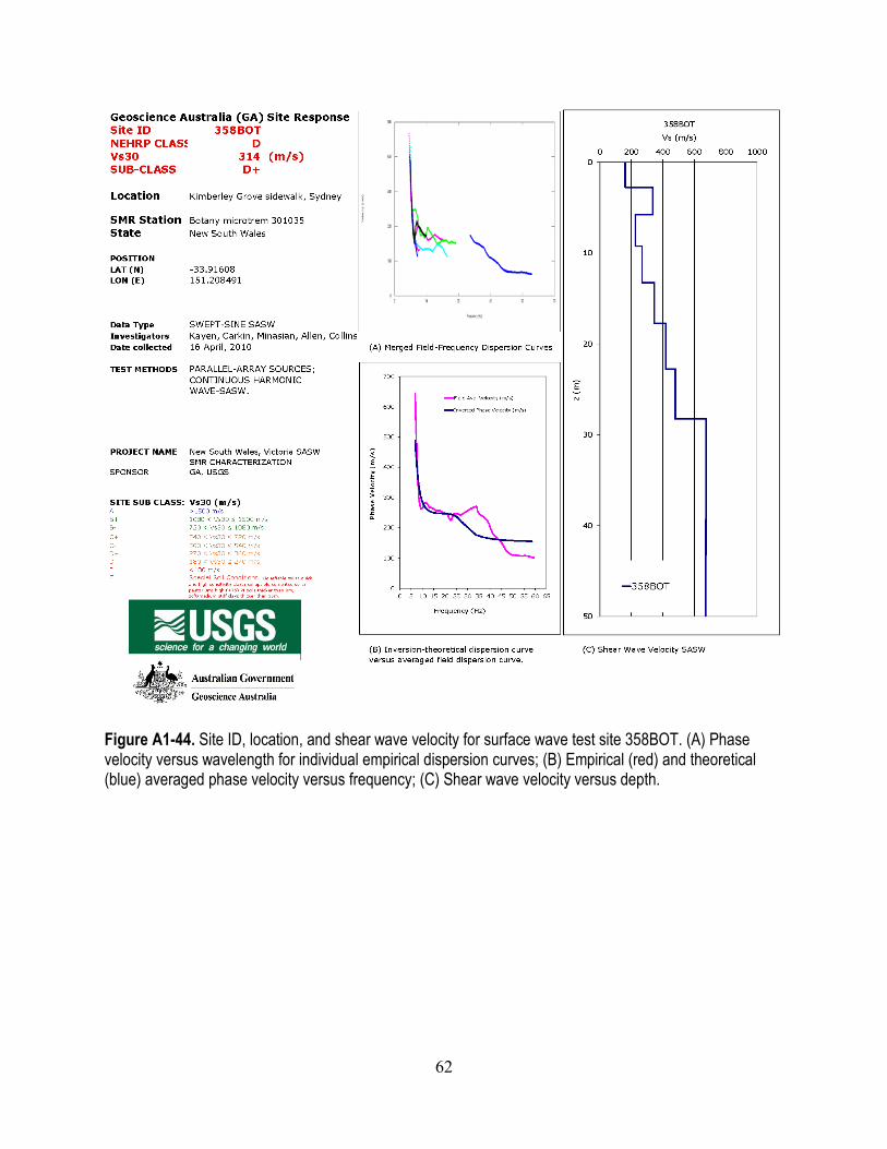
Figure A1-44. Site ID, location, and shear wave velocity for surface wave test site 358BOT. (A) Phase velocity versus wavelength for individual empirical dispersion curves; (B) Empirical (red) and theoretical (blue) averaged phase velocity versus frequency; (C) Shear wave velocity versus depth.

63
Figure A1-45. Surface wave test site 359RIV located at Saint Ignatius’ College, Riverview, northeastern suburbs, Sydney, New South Wales (lat -33.8277, long 151.1591). Tested on April 17, 2010. (A) view looking west from the shakers; (B) another view looking west from the shakers; (C) view east to the shakers; (D) view to the NW into play field adjacent to the test area; (E) satellite view of the local site, red and white symbol is the location of the shakers, the yellow bar is the seismometer array; (F) site location in New South Wales.

64
Figure A1-46. Site ID, location, and shear wave velocity for surface wave test site 359RIV. (A) Phase velocity versus wavelength for individual empirical dispersion curves; (B) Empirical (red) and theoretical (blue) averaged phase velocity versus frequency; (C) Shear wave velocity versus depth.

65
Figure A1-47. Surface wave test site 360BOT, Botany, southern suburbs, Sydney, New South Wales (lat -33.93928, long 151.20146). Botany microtremor site 305054, tested on April 17, 2010. (A) view looking southward from the shakers; (B) view northwards to the shakers; (C) view SW from shakers; (D) view southward along the seismometer array; (E) satellite view of the local site, red and white symbol is the location of the shakers, the yellow bar is the seismometer array; (F) site location in New South Wales.

66
Figure A1-48. Site ID, location, and shear wave velocity for surface wave test site 360BOT. (A) Phase velocity versus wavelength for individual empirical dispersion curves; (B) Empirical (red) and theoretical (blue) averaged phase velocity versus frequency; (C) Shear wave velocity versus depth.

67
Figure A1-49. Surface wave test site 361BOT located at Sir Joseph Banks Park, Banksmeadow, southern suburbs, Sydney, New South Wales (lat -33.9556, long 151.20241). Botany microtremor site 304052, tested on April 17, 2010. (A) view to the SE from the shakers; (B) view NW along the seismometer array; (C) view SE from near the shakers; (D) view to the NE near the shakers; (E) satellite view of the local site, red and white symbol is the location of the shakers, the yellow bar is the seismometer array; (F) site location in New South Wales.

68
Figure A1-50. Site ID, location, and shear wave velocity for surface wave test site 361BOT. (A) Phase velocity versus wavelength for individual empirical dispersion curves; (B) Empirical (red) and theoretical (blue) averaged phase velocity versus frequency; (C) Shear wave velocity versus depth.

69
Figure A1-51. Surface wave test site 362BOT located at Botany Golf Club, Banksmeadow, southern suburbs, Sydney, New South Wales (lat -33.9585, long 151.20706). Botany microtremor site 30036, tested on April 19, 2010. (A) view looking NW along the seismometer array from the shakers; (B) another view NW from near the shakers; (C) view SE toward the shakers; (D) view NW to the shakers and seismometer array; (E) satellite view of the local site, red and white symbol is the location of the shakers, the yellow bar is the seismometer array; (F) site location in New South Wales.

70
Figure A1-52. Site ID, location, and shear wave velocity for surface wave test site 362BOT. (A) Phase velocity versus wavelength for individual empirical dispersion curves; (B) Empirical (red) and theoretical (blue) averaged phase velocity versus frequency; (C) Shear wave velocity versus depth.

71
Figure A1-53. Surface wave test site 363NEW located at Wickham Park, Wickham district, Newcastle, New South Wales (lat -32.9189, long 151.7556). Wik-01 SCPT-36.0 m site, tested on April 20, 2010. (A) view to the north from the shakers; (B) view SW from the shakers; (C) another view SW from the shakers; (D) view to the NW along the seismometer array; (E) satellite view of the local site, red and white symbol is the location of the shakers, the yellow bar is the seismometer array; (F) site location in New South Wales.

72
Figure A1-54. Site ID, location, and shear wave velocity for surface wave test site 363NEW. (A) Phase velocity versus wavelength for individual empirical dispersion curves; (B) Empirical (red) and theoretical (blue) averaged phase velocity versus frequency; (C) Shear wave velocity versus depth.

73
Figure A1-55. Surface wave test site 364NEW located at Islington Park, Islington district, Newcastle, New South Wales (lat -32.91053, long 151.74651). Iso-01 SCPT-15.0 m site, tested on April 20, 2010. (A) view looking southward along seismometer array from the shakers; (B) view northward to the shakers; (C) view SE across seismometer array toward Styx Creek; (D) view to the west near the shakers; (E) satellite view of the local site, red and white symbol is the location of the shakers, the yellow bar is the seismometer array; (F) site location in New South Wales.

74
Figure A1-56. Site ID, location, and shear wave velocity for surface wave test site 364NEW. (A) Phase velocity versus wavelength for individual empirical dispersion curves; (B) Empirical (red) and theoretical (blue) averaged phase velocity versus frequency; (C) Shear wave velocity versus depth.

75
Figure A1-57. Surface wave test site 365NEW, North Lambton district, Newcastle, New South Wales (lat -32.90133, long 151.70391). North Lambton Depot-JUMP ES&S site, tested on April 20,2010. (A) view westward from the shakers; (B) view SE from the shakers; (C) view to the NE from across Compton Street toward the shakers; (D) view to the west along Compton Street; (E) satellite view of the local site, red and white symbol is the location of the shakers, the yellow bar is the seismometer array; (F) site location in New South Wales.
76
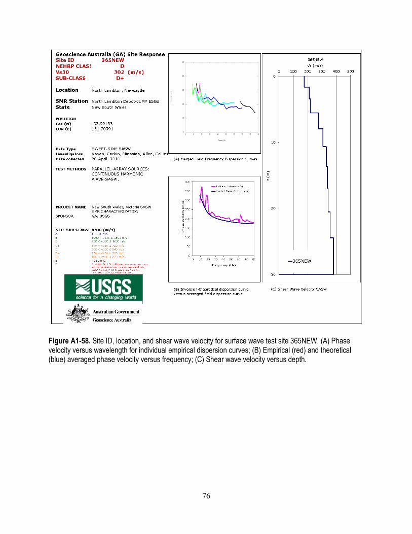
Figure A1-58. Site ID, location, and shear wave velocity for surface wave test site 365NEW. (A) Phase velocity versus wavelength for individual empirical dispersion curves; (B) Empirical (red) and theoretical (blue) averaged phase velocity versus frequency; (C) Shear wave velocity versus depth.

77
Figure A1-59. Surface wave test site 366NEW located at Smith Park, Broadmeadow district, Newcastle, New South Wales (lat -32.91661, long 151.73515). Brd-04 SCPT-26.7 m site, tested on April 20, 2010. (A) view looking northward from shakers; (B) view SE from the shakers; (C) view north across Smith Park; (D) view to the NE from near the shakers; (E) satellite view of the local site, red and white symbol is the location of the shakers, the yellow bar is the seismometer array; (F) site location in New South Wales.

78
Figure A1-60. Site ID, location, and shear wave velocity for surface wave test site 366NEW. (A) Phase velocity versus wavelength for individual empirical dispersion curves; (B) Empirical (red) and theoretical (blue) averaged phase velocity versus frequency; (C) Shear wave velocity versus depth.

79
Figure A1-61. Surface wave test site 367NEW located at Darling Street Oval, Broadmeadow district, Newcastle, New South Wales (lat -32.9343, long 151.7402). Brd-09 SCPT site-11.5 m, tested on April 21, 2010. (A) view looking north from shakers; (B) view south toward the shakers; (C) view SE toward shakers; (D) view to the SW toward the shakers; (E) satellite view of the local site, red and white symbol is the location of the shakers, the yellow bar is the seismometer array; (F) site location in New South Wales.

80
Figure A1-62. Site ID, location, and shear wave velocity for surface wave test site 367NEW. (A) Phase velocity versus wavelength for individual empirical dispersion curves; (B) Empirical (red) and theoretical (blue) averaged phase velocity versus frequency; (C) Shear wave velocity versus depth.

81
Figure A1-63. Surface wave test site 368NEW located at Henderson Park, Merewether district, Newcastle, New South Wales (lat -32.93837, long 151.73731). Mer-05 SCPT-6.8 m site, tested on April 21, 2010. (A) view looking NE from the shakers; (B) another view to the NE down the seismometer array; (C) view SE to the shakers; (D) view to the SE across the park toward the shakers; (E) satellite view of the local site, red and white symbol is the location of the shakers, the yellow bar is the seismometer array; (F) site location in New South Wales.

82
Figure A1-64. Site ID, location, and shear wave velocity for surface wave test site 368NEW. (A) Phase velocity versus wavelength for individual empirical dispersion curves; (B) Empirical (red) and theoretical (blue) averaged phase velocity versus frequency; (C) Shear wave velocity versus depth.

83
Figure A1-65. Surface wave test site 369MNG located 1.3 km NW of Mangrove Creek Dam, New South Wales (lat -33.2094, long 151.1093). Mangrove Creek ANSN site, tested on April 21, 2010. (A) view looking W-NW from the dam towards the shaker location (red circle) on the ridgetop; (B) view southward on the ridgetop toward the shakers; (C) view eastward from near the shakers toward the ANSN seismometer location; (D) ANSN seismometer and solar panels on ridgetop; (E) satellite view of the local site, red and white symbol is the location of the shakers, the yellow bar is the seismometer array; (F) site location in New South Wales.
84
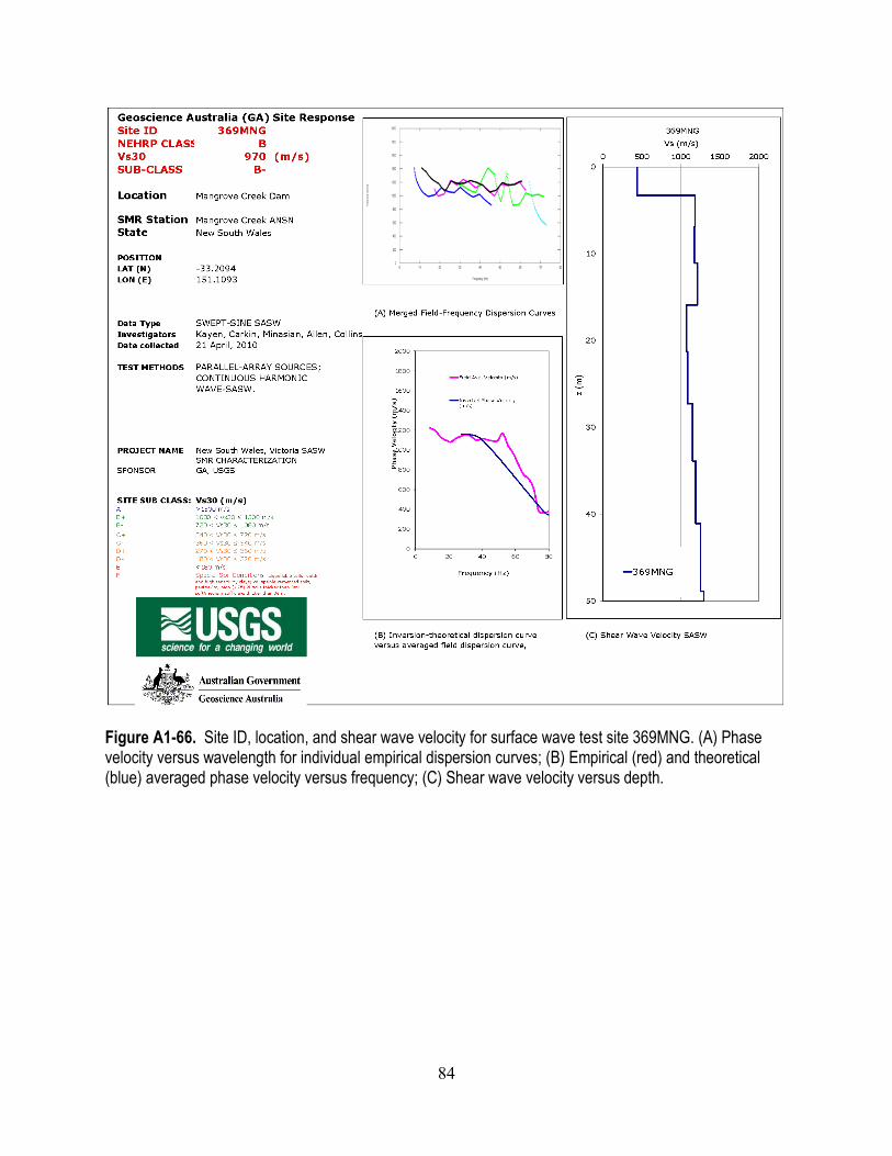
Figure A1-66. Site ID, location, and shear wave velocity for surface wave test site 369MNG. (A) Phase velocity versus wavelength for individual empirical dispersion curves; (B) Empirical (red) and theoretical (blue) averaged phase velocity versus frequency; (C) Shear wave velocity versus depth.

85
Figure A1-67. Surface wave test site 370LYG, Loy Yang, located about 7 km S-SW of Traralgon, Victoria (lat -38.26627, long 146.50835). Latrobe HHF Loy Yang site, tested on April 23, 2010. (A) view to the NW toward the shakers; (B) two shakers in operation at the test site; (C) satellite view of the surrounding region; (D) satellite view of the local site, red and white symbol is the location of the shakers, the yellow bar is the seismometer array; (E) site location in Victoria.

86
Figure A1-68. Site ID, location, and shear wave velocity for surface wave test site 370LYG. (A) Phase velocity versus wavelength for individual empirical dispersion curves; (B) Empirical (red) and theoretical (blue) averaged phase velocity versus frequency; (C) Shear wave velocity versus depth.

87
Figure A1-69. Surface wave test site 371RSD located 1 km northeast of Rosedale, Gippsland, Victoria (lat -38.14317, long 146.79073). Latrobe alluvium-Rosedale site, tested on April 24, 2010. (A) view looking north at the shakers; (B) another view looking north to the shakers; (C) view south from the shakers down the seismometer array; (D) another view to the south to the site location; (E) satellite view of the local site, red and white symbol is the location of the shakers, the yellow bar is the seismometer array; (F) site location in Victoria.

88
Figure A1-70. Site ID, location, and shear wave velocity for surface wave test site 371RSD. (A) Phase velocity versus wavelength for individual empirical dispersion curves; (B) Empirical (red) and theoretical (blue) averaged phase velocity versus frequency; (C) Shear wave velocity versus depth.
89
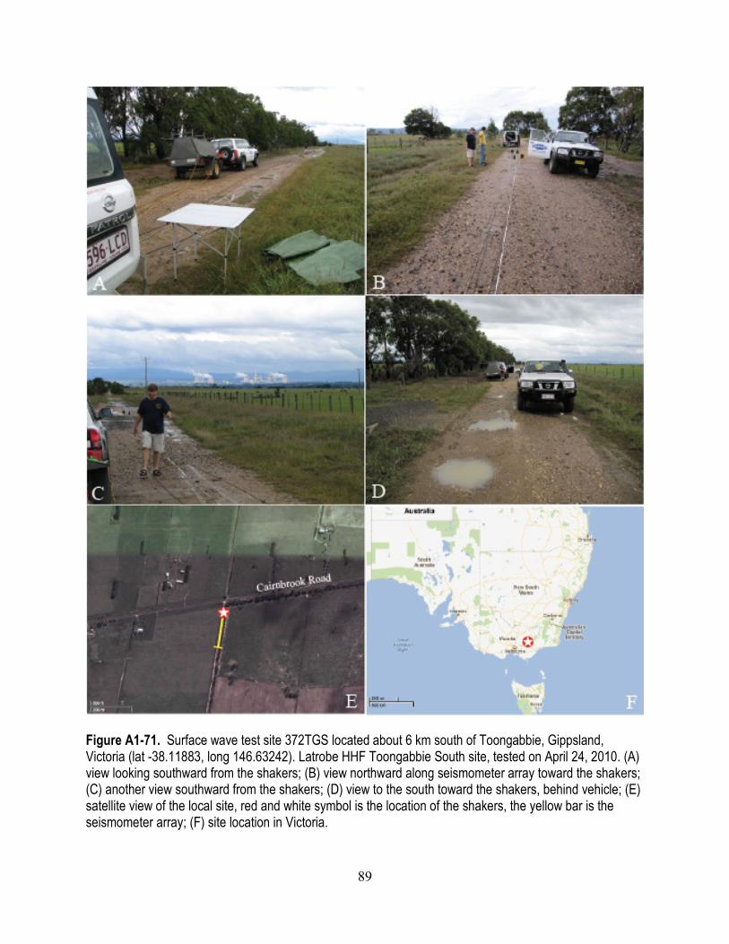
Figure A1-71. Surface wave test site 372TGS located about 6 km south of Toongabbie, Gippsland, Victoria (lat -38.11883, long 146.63242). Latrobe HHF Toongabbie South site, tested on April 24, 2010. (A) view looking southward from the shakers; (B) view northward along seismometer array toward the shakers; (C) another view southward from the shakers; (D) view to the south toward the shakers, behind vehicle; (E) satellite view of the local site, red and white symbol is the location of the shakers, the yellow bar is the seismometer array; (F) site location in Victoria.

90
Figure A1-72. Site ID, location, and shear wave velocity for surface wave test site 372TGS. (A) Phase velocity versus wavelength for individual empirical dispersion curves; (B) Empirical (red) and theoretical (blue) averaged phase velocity versus frequency; (C) Shear wave velocity versus depth.

91
Figure A1-73. Surface wave test site 373TGB located 5 km NE of Toongabbie, Gippsland, Victoria (lat -38.02631, long 146.66515). Latrobe HHF Toongabbie site, tested on April 24, 2010. (A) view looking eastward down the seismometer array from the shakers; (B) view westward from from the shakers; (C) another view westward from shakers; (D) view NE from the shakers; (E) satellite view of the local site, red and white symbol is the location of the shakers, the yellow bar is the seismometer array; (F) site location in Victoria.

92
Figure A1-74. Site ID, location, and shear wave velocity for surface wave test site 373TGB. (A) Phase velocity versus wavelength for individual empirical dispersion curves; (B) Empirical (red) and theoretical (blue) averaged phase velocity versus frequency; (C) Shear wave velocity versus depth.

93
Figure A1-75. Surface wave test site 374NAM located about 3 km west of Nambrok, Victoria (lat -38.05449, long 146.83669). Latrobe HHF-Nambrok West site, tested on April 24, 2010. (A) view looking southward from the shakers; (B) view northward from the shakers to the seismometer array along Nambrok Road; (C) satellite view of the surrounding area; (D) satellite view of the local site, red and white symbol is the location of the shakers, the yellow bar is the seismometer array; (E) site location in Victoria.

94
Figure A1-76. Site ID, location, and shear wave velocity for surface wave test site 374NAM. (A) Phase velocity versus wavelength for individual empirical dispersion curves; (B) Empirical (red) and theoretical (blue) averaged phase velocity versus frequency; (C) Shear wave velocity versus depth.

95
Figure A1-77. Surface wave test site 375GFW, Giffard West, located 8.4 km NW of Giffard, Victoria (lat -38.37931, long 146.99754). Pleistocene dunes Giffard West site, tested on April 25, 2010. (A) view looking westward in the direction of the seismometer array; (B) view eastward from the shakers; (C) another view eastward from the shakers; (D) view to the SW from the shakers; (E) satellite view of the local site, red and white symbol is the location of the shakers, the yellow bar is the seismometer array; (F) site location in Victoria.

96
Figure A1-78. Site ID, location, and shear wave velocity for surface wave test site 375GFW. (A) Phase velocity versus wavelength for individual empirical dispersion curves; (B) Empirical (red) and theoretical (blue) averaged phase velocity versus frequency; (C) Shear wave velocity versus depth.

97
Figure A1-79. Surface wave test site 376LNF located about 10 km west of Sale, Victoria (lat -38.10309, long 146.95038). Latrobe HHF Kilmany site, tested on April 25, 2010. (A) view looking west from the shakers; (B) view SW to the shakers; (C) view SE to the shakers; (D) view southward to the shakers; (E) satellite view of the local site, red and white symbol is the location of the shakers, the yellow bars are the seismometer arrays, spacings up to 50 meters oriented E-W, 87-meter spacing oriented N-NE; (F) site location in Victoria.

98
Figure A1-80. Site ID, location, and shear wave velocity for surface wave test site 376LNF. (A) Phase velocity versus wavelength for individual empirical dispersion curves; (B) Empirical (red) and theoretical (blue) averaged phase velocity versus frequency; (C) Shear wave velocity versus depth.
99
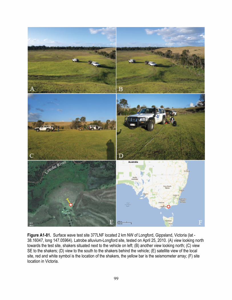
Figure A1-81. Surface wave test site 377LNF located 2 km NW of Longford, Gippsland, Victoria (lat -38.16047, long 147.05964). Latrobe alluvium-Longford site, tested on April 25, 2010. (A) view looking north towards the test site, shakers situated next to the vehicle on left; (B) another view looking north; (C) view SE to the shakers; (D) view to the south to the shakers behind the vehicle; (E) satellite view of the local site, red and white symbol is the location of the shakers, the yellow bar is the seismometer array; (F) site location in Victoria.

100
Figure A1-82. Site ID, location, and shear wave velocity for surface wave test site 377LNF. (A) Phase velocity versus wavelength for individual empirical dispersion curves; (B) Empirical (red) and theoretical (blue) averaged phase velocity versus frequency; (C) Shear wave velocity versus depth.
101
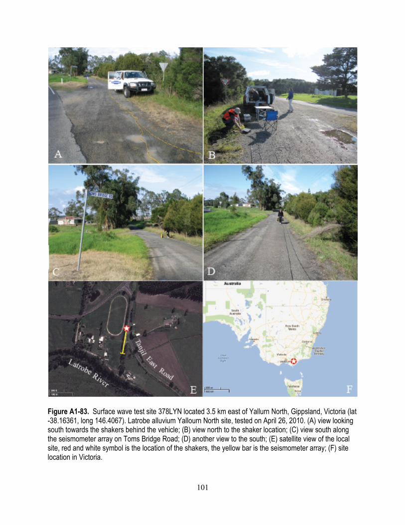
Figure A1-83. Surface wave test site 378LYN located 3.5 km east of Yallurn North, Gippsland, Victoria (lat -38.16361, long 146.4067). Latrobe alluvium Yallourn North site, tested on April 26, 2010. (A) view looking south towards the shakers behind the vehicle; (B) view north to the shaker location; (C) view south along the seismometer array on Toms Bridge Road; (D) another view to the south; (E) satellite view of the local site, red and white symbol is the location of the shakers, the yellow bar is the seismometer array; (F) site location in Victoria.

102
Figure A1-84. Site ID, location, and shear wave velocity for surface wave test site 378YLN. (A) Phase velocity versus wavelength for individual empirical dispersion curves; (B) Empirical (red) and theoretical (blue) averaged phase velocity versus frequency; (C) Shear wave velocity versus depth.

103
Figure A1-85. Surface wave test site 379GLG located 3.5 km S-SW of Glengarry, Gippsland, Victoria (lat -38.16161, long 146.5567). Latrobe alluvium-Glengarry site, tested on April 26, 2010. (A) view looking SE towards the shakers behind the vehicles; (B) view to the east to the shaker location; (C) view SE from shakers down the seismometer array; (D) satellite view of the local site, red and white symbol is the location of the shakers, the yellow bar is the seismometer array; (E) site location in Victoria.

104
Figure A1-86. Site ID, location, and shear wave velocity for surface wave test site 379GLG. (A) Phase velocity versus wavelength for individual empirical dispersion curves; (B) Empirical (red) and theoretical (blue) averaged phase velocity versus frequency; (C) Shear wave velocity versus depth.

105
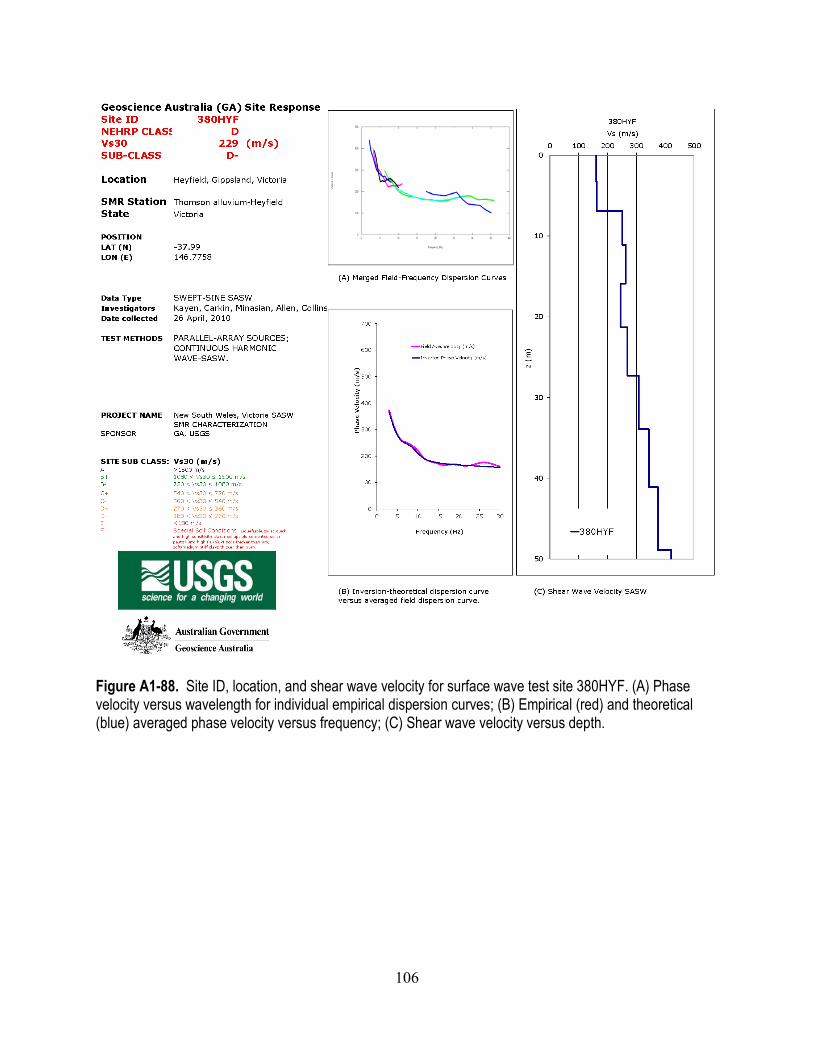
Figure A1-87. Surface wave test site 380HYF located about 1 km SW of Heyfield, Gippsland, Victoria (lat -37.9900, long 146.7758). Thomson alluvium Heyfield site, tested on April 26, 2010. (A) view looking west from the shakers; (B) another view looking westward; (C) view west down the dirt road and seismometer array; (D) view of the site looking west from the Traralgon-Maffra Road; (E) satellite view of the local site, red and white symbol is the location of the shakers, the yellow bar is the seismometer array; (F) site location in Victoria.
106
Figure A1-88. Site ID, location, and shear wave velocity for surface wave test site 380HYF. (A) Phase velocity versus wavelength for individual empirical dispersion curves; (B) Empirical (red) and theoretical (blue) averaged phase velocity versus frequency; (C) Shear wave velocity versus depth.
107
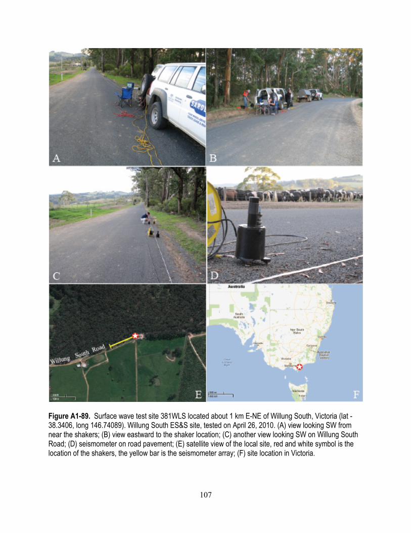
Figure A1-89. Surface wave test site 381WLS located about 1 km E-NE of Willung South, Victoria (lat -38.3406, long 146.74089). Willung South ES&S site, tested on April 26, 2010. (A) view looking SW from near the shakers; (B) view eastward to the shaker location; (C) another view looking SW on Willung South Road; (D) seismometer on road pavement; (E) satellite view of the local site, red and white symbol is the location of the shakers, the yellow bar is the seismometer array; (F) site location in Victoria.

108
Figure A1-90. Site ID, location, and shear wave velocity for surface wave test site 381WLS. (A) Phase velocity versus wavelength for individual empirical dispersion curves; (B) Empirical (red) and theoretical (blue) averaged phase velocity versus frequency; (C) Shear wave velocity versus depth.

109
Figure A1-91. Surface wave test site 382THD located 5.5 km NW of Thomson Dam, Victoria (lat -37.80987, long 146.35046). Thomson Dam ES&S site, tested on April 27, 2010. (A) view towards the north from shakers; (B) view south to the shakers and ES&S seismometer shed beyond vehicle; (C) another view south to the ES&S seismometer shed beyond vehicle; (D) view to the north from the ES&S seismometer shed; (E) satellite view of the local site, red and white symbol is the location of the shakers, the yellow bar is the seismometer array; (F) site location in Victoria.

110
Figure A1-92. Site ID, location, and shear wave velocity for surface wave test site 382THD. (A) Phase velocity versus wavelength for individual empirical dispersion curves; (B) Empirical (red) and theoretical (blue) averaged phase velocity versus frequency; (C) Shear wave velocity versus depth.
111
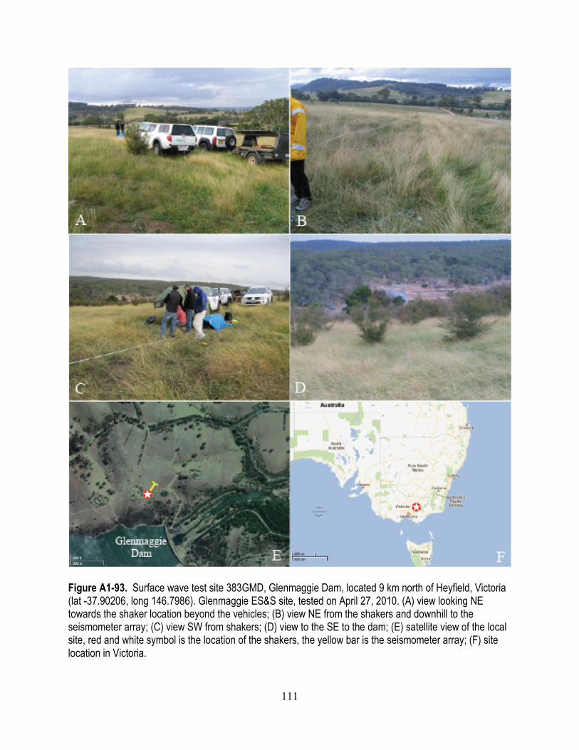
Figure A1-93. Surface wave test site 383GMD, Glenmaggie Dam, located 9 km north of Heyfield, Victoria (lat -37.90206, long 146.7986). Glenmaggie ES&S site, tested on April 27, 2010. (A) view looking NE towards the shaker location beyond the vehicles; (B) view NE from the shakers and downhill to the seismometer array; (C) view SW from shakers; (D) view to the SE to the dam; (E) satellite view of the local site, red and white symbol is the location of the shakers, the yellow bar is the seismometer array; (F) site location in Victoria.

112
Figure A1-94. Site ID, location, and shear wave velocity for surface wave test site 383GMD. (A) Phase velocity versus wavelength for individual empirical dispersion curves; (B) Empirical (red) and theoretical averaged phase velocity (blue) versus frequency; (C) Shear wave velocity versus depth.

113
Figure A1-95. Surface wave test site 384TLG located 4 km S-SE of Toolangi, Victoria (lat -37.56952, long 145.49085). Toolangi ANSN site, tested on April 28, 2010. (A) view looking east toward the shakers and seismometer array; (B) view westward toward the shakers; (C) view westward to shakers and ANSN seismometer station within fenced area; (D) sign on fence; (E) satellite view of the local site, red and white symbol is the location of the shakers, the yellow bar is the seismometer array; (F) site location in Victoria.
114
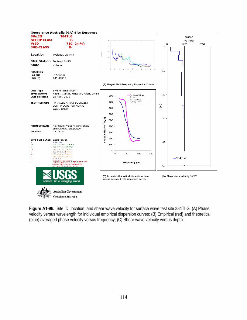
Figure A1-96. Site ID, location, and shear wave velocity for surface wave test site 384TLG. (A) Phase velocity versus wavelength for individual empirical dispersion curves; (B) Empirical (red) and theoretical (blue) averaged phase velocity versus frequency; (C) Shear wave velocity versus depth.

115
Figure A1-97. Surface wave test site 385GRV located at Greenvale, Victoria (lat -37.61685, long 144.90262). Greenvale ES&S site, tested on April 28, 2010. (A) view looking NW towards the shakers and the seismometer array; (B) another view NW to the seismometer array; (C) view southward from the shakers toward the green ES&S seismometer shelter (red arrow); (D) view to the SE to the shakers; (E) satellite view of the local site, red and white symbol is the location of the shakers, the yellow bar is the seismometer array, red arrow indicates the location of the ES&S seismometer; (F) site location in Victoria.

116
Figure A1-98. Site ID, location, and shear wave velocity for surface wave test site 385GRV. (A) Phase velocity versus wavelength for individual empirical dispersion curves; (B) Empirical (red) and theoretical (blue) averaged phase velocity versus frequency; (C) Shear wave velocity versus depth

117
Figure A1-99. Surface wave test site 386FCR located about 10 km SW of Fish Creek, Victoria (lat -38.75622, long 146.0001). Fish Creek ES&S site, tested on April 29, 2010. (A) view looking NE from the shakers uphill toward the seismometer array; (B) view SW toward the shakers; (C) view SE from the shakers; (D) satellite view of the local site, red and white symbol is the location of the shakers, the yellow bar is the seismometer array; (E) site location in Victoria.
118
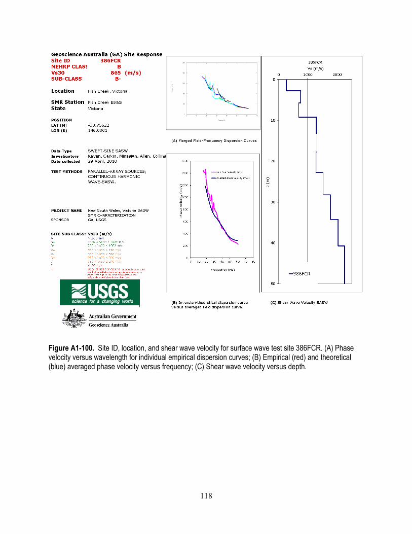
Figure A1-100. Site ID, location, and shear wave velocity for surface wave test site 386FCR. (A) Phase velocity versus wavelength for individual empirical dispersion curves; (B) Empirical (red) and theoretical (blue) averaged phase velocity versus frequency; (C) Shear wave velocity versus depth.

Publishing support provided by the U.S. Geological Survey SciencePublishing Network, Menlo Park and Tacoma Publishing Service Centers
For more information concerning the research in this report, contact the U.S. Geological Survey Pacific Science Center 400 Natural Bridges Drive Santa Cruz, CA 95060 http://walrus.wr.usgs.gov/

Kayen and others—Shear-W
ave Velocity and Site-Am
plification Factors for 50 Australian Sites D
etermined by the Spectral A
nalysis of Surface Waves M
ethod—Open-File Report 2014–1264
ISSN 2331-1258 (online)http://dx.doi.org/10.3133/ofr20141264