Embed Size (px)
Citation preview

arX
iv:0
809.
2144
v1 [
nucl
-th]
12
Sep
2008
Shell-model calculations and realistic effective interactions
L. Coraggio1, A. Covello1,2, A. Gargano1, N. Itaco1,2 and T. T. S. Kuo3
1 Istituto Nazionale di Fisica Nucleare,Complesso Universitario di Monte S. Angelo, Via Cintia, I-80126 Napoli, Italy
2 Dipartimento di Scienze Fisiche, Universita di Napoli Federico II,Complesso Universitario di Monte S. Angelo, Via Cintia, I-80126 Napoli, Italy
3 Department of Physics, SUNY, Stony Brook, New York 11794, USA
May 25, 2018
Abstract
A review is presented of the development and current status of nuclear shell-model calculations
in which the two-body effective interaction between the valence nucleons is derived from the free
nucleon-nucleon potential. The significant progress made in this field within the last decade is
emphasized, in particular as regards the so-called Vlow−k approach to the renormalization of the
bare nucleon-nucleon interaction. In the last part of the review we first give a survey of realistic
shell-model calculations from early to present days. Then, we report recent results for neutron-rich
nuclei near doubly magic 132Sn and for the whole even-mass N = 82 isotonic chain. These illustrate
how shell-model effective interactions derived from modern nucleon-nucleon potentials are able to
provide an accurate description of nuclear structure properties.
Contents
1 Introduction 2
2 Nucleon-nucleon interaction 6
2.1 Historical overview . . . . . . . . . . . . . . . . . . . . . . . . . . . . . . . . . . . . . . 62.2 High-precision NN potentials . . . . . . . . . . . . . . . . . . . . . . . . . . . . . . . . 82.3 Chiral potentials . . . . . . . . . . . . . . . . . . . . . . . . . . . . . . . . . . . . . . . 10
3 Shell-model effective interaction 12
3.1 Generalities . . . . . . . . . . . . . . . . . . . . . . . . . . . . . . . . . . . . . . . . . . 123.2 Degenerate time-dependent perturbation theory: folded-diagram approach . . . . . . . 14
3.2.1 Folded diagrams . . . . . . . . . . . . . . . . . . . . . . . . . . . . . . . . . . . . 143.2.2 The decomposition theorem . . . . . . . . . . . . . . . . . . . . . . . . . . . . . 173.2.3 The model-space secular equation . . . . . . . . . . . . . . . . . . . . . . . . . . 20
3.3 The Lee-Suzuki method . . . . . . . . . . . . . . . . . . . . . . . . . . . . . . . . . . . 24
4 Handling the short-range repulsion of the NN potential 25
4.1 The Brueckner G-matrix approach . . . . . . . . . . . . . . . . . . . . . . . . . . . . . 264.1.1 Historical introduction . . . . . . . . . . . . . . . . . . . . . . . . . . . . . . . . 264.1.2 Essentials of the theory . . . . . . . . . . . . . . . . . . . . . . . . . . . . . . . . 27
1
4.1.3 Calculation of the reaction matrix . . . . . . . . . . . . . . . . . . . . . . . . . . 324.2 The Vlow−k approach . . . . . . . . . . . . . . . . . . . . . . . . . . . . . . . . . . . . . 34
4.2.1 Derivation of the low-momentum NN potential 1 Vlow−k . . . . . . . . . . . . . 344.2.2 Phase-shift equivalent Hermitian Vlow−k’s . . . . . . . . . . . . . . . . . . . . . . 374.2.3 Properties of Vlow−k . . . . . . . . . . . . . . . . . . . . . . . . . . . . . . . . . . 40
5 Realistic shell-model calculations 45
5.1 The early period . . . . . . . . . . . . . . . . . . . . . . . . . . . . . . . . . . . . . . . 455.2 Modern calculations . . . . . . . . . . . . . . . . . . . . . . . . . . . . . . . . . . . . . 485.3 Results . . . . . . . . . . . . . . . . . . . . . . . . . . . . . . . . . . . . . . . . . . . . . 49
5.3.1 Comparison between G-matrix and Vlow−k approaches . . . . . . . . . . . . . . . 495.3.2 Calculations with different NN potentials . . . . . . . . . . . . . . . . . . . . . 515.3.3 Neutron rich nuclei beyond 132Sn: comparing theory and experiment . . . . . . . 545.3.4 The role of many-body forces . . . . . . . . . . . . . . . . . . . . . . . . . . . . 57
6 Summary and conclusions 59
1 Introduction
The shell model is the basic framework for nuclear structure calculations in terms of nucleons. Thismodel, which entered into nuclear physics more than fifty years ago [1, 2], is based on the assumptionthat, as a first approximation, each nucleon inside the nucleus moves independently from the others ina spherically symmetric potential including a strong spin-orbit term. Within this approximation thenucleus is considered as an inert core, made up by shells filled up with neutrons and protons paired toangular momentum J = 0, plus a certain number of external nucleons, the “valence” nucleons. As iswell known, this extreme single-particle shell model, supplemented by empirical coupling rules, provedvery soon to be able to account for various nuclear properties [3], like the angular momentum andparity of the ground-states of odd-mass nuclei. It was clear from the beginning [4], however, that fora description of nuclei with two or more valence nucleons the “residual” two-body interaction betweenthe valence nucleons had to be taken explicitly into account, the term residual meaning that part of theinteraction which is not absorbed into the central potential. This removes the degeneracy of the statesbelonging to the same configuration and produces a mixing of different configurations. A fascinatingaccount of the early stages of the nuclear shell model is given in the comprehensive review by Talmi [5].
In any shell-model calculation one has to start by defining a “model space”, namely by specifyinga set of active single-particle (SP) orbits. It is in this truncated Hilbert space that the Hamiltonianmatrix has to be set up and diagonalized. A basic input, as mentioned above, is the residual interactionbetween valence nucleons. This is in reality a “model-space effective interaction”, which differs fromthe interaction between free nucleons in various respects. In fact, besides being residual in the sensementioned above, it must account for the configurations excluded from the model space.
It goes without saying that a fundamental goal of nuclear physics is to understand the properties ofnuclei starting from the forces between nucleons. Nowadays, the A nucleons in a nucleus are understoodas non-relativistic particles interacting via a Hamiltonian consisting of two-body, three-body, and higher-body potentials, with the nucleon-nucleon (NN) term being the dominant one.
In this context, it is worth emphasizing that there are two main lines of attack to attain this ambitiousgoal. The first one is comprised of the so-called ab initio calculations where nuclear properties, such asbinding and excitation energies, are calculated directly from the first principles of quantum mechanicsusing appropriate computational scheme. To this category belong the Green’s function MontecarloMethod (GFMC) [6, 7], the no-core shell-model (NCSM)) [8, 9], and the coupled-cluster methods(CCM)) [10, 11]. The GFMC calculations, on which we shall briefly comment in Sec. 2.3, are at
2
present limited to nuclei with A ≤ 12. This limit may be overcome by using limited Hilbert spacesand introducing effective interactions, which is done in the NCSM and CCM. Actually, coupled-clustercalculations employing modern NN potentials have been recently performed for 16O and its immediateneighbours [12, 13, 14].
The main feature of the NCSM is the use of a large, but finite number of harmonic oscillatorbasis states to diagonalize an effective Hamiltonian containing realistic two- and three- nucleon inter-actions [15]. In this way, no closed core is assumed and all nucleons in the nucleus are treated as activeparticles. Very recently, this approach has ben applied to the study of A = 10− 13 nuclei [16]. Clearly,all ab initio calculations need huge amount of computational resources and therefore, as mentionedabove, are currently limited to light nuclei.
The second line of attack is just the theme of this review paper, namely the use of the traditionalshell-model with two-nucleon effective interactions derived from the bare NN potential. In this case,only the valence nucleons are treated as active particles. However, as we shall discuss in detail inSec.. 3, core polarization effects are taken into account perturbatively in the derivation of the effectiveinteraction. Of course, this approach allows to perform calculations for medium- and heavy-mass nucleiwhich are far beyond the reach of ab initio calculations. Many-body forces beyond the NN potentialmay also play a role in the shell-model effective Hamiltonian. However, this is still an open problemand it is the main scope of this review to assess t he progress made in the derivation of a two-bodyeffective interaction from the free NN potential.
While efforts in this direction started some forty years ago [17, 18], for a long time there waswidespread skepticism about the practical value of what had become known as “realistic shell model”calculations. This was mainly related to the highly complicated nature of the nucleon-nucleon force, inparticular to the presence of a very strong repulsion at short distances, which made especially difficultsolving the nuclear many-body problem. As a consequence, a major problem, and correspondingly amain source of uncertainty, in shell-model calculations has long been the two-body effective interactionbetween the valence nucleons. An early survey of the various approaches to this problem can be foundin the Cargese lectures by Elliott [19], where a classification of the various categories of nuclear structurecalculations was made by the number of free parameters in the two-body interaction being used in thecalculation.
Since the early 1950s through the mid 1990s hundreds of shell-model calculations have been carriedout, many of them being very successful in describing a variety of nuclear structure phenomena. In thevast majority of these calculations either empirical effective interactions containing adjustable parame-ters have been used or the two body-matrix elements themselves have been treated as free parameters.The latter approach, which was pioneered by Talmi [20], is generally limited to relatively small spacesowing to the large number of parameters to be least-squares fitted to experimental data.
Early calculations of this kind were performed for the p-shell nuclei by Cohen and Kurath [21], whodetermined fifteen matrix elements of the two-body interaction and two single-particle energies from 35experimental energies of nuclei from A = 8 up to A = 16. The results of these calculations turned outto be in very satisfactory agreement with experiment.
A more recent and very successful application of this approach is that by Brown and Wildenthal[22, 23, 24], where the A = 17 − 39 nuclei were studied in the complete sd-shell space. In the finalversion of this study, which spanned about 10 years, 66 parameters were determined by a least squaresfit to 447 binding and excitation energies. A measure of the quality of the results is given by therms deviation, whose value turned out to be 185 keV. In this connection, it is worth mentioning thatin the recent work of Brown and Richter [25] the determination of a new effective interaction for thesd-shell has been pursued by the inclusion of an updated set of experimental data. As regards theempirical effective interactions, they may be schematically divided into two categories. The first isbased on the use of simple potentials such as a Gaussian or Yukawa central force with various exchangeoperators consistent with those present in the interaction between free nucleons. These contain several
3

parameters, such as the strengths and ranges of the singlet and triplet interactions, which are usuallydetermined by a fit to the spectroscopic properties under study. In the second category one may putthe so-called “schematic interactions”. These contain few free parameters, typically one or two, at theprice of being an oversimplified representation of the real potential. Into this category fall the wellknown pairing [26, 27, 28], pairing plus quadrupole [29], and surface delta [30, 31, 32] interactions. Thesuccessful spin and isospin dependent Migdal interaction [33] also belongs to this category. While thesesimple interactions are able to reproduce some specific nuclear properties [see, e.g., [34, 35]], they areclearly inadequate for detailed quantitative studies.
We have given above a brief sketch of the various approaches to the determination of the shell-modeleffective interaction that have dominated the field for more than four decades. This we have done toplace in its proper perspective the great progress made over the last decade by the more fundamentalapproach employing realistic effective interactions derived from modern NN potentials. We refer toRef. [5] for a detailed review of shell-model calculations based on the above empirical approaches.
As we shall discuss in detail in the following sections, from the late 1970s on there has been sub-stantial progress toward a microscopic approach to nuclear structure calculations starting from the freeNN potential VNN . This has concerned both the two basic ingredients which come into play in thisapproach, namely the NN potential and the many-body methods for deriving the model space effectiveinteraction, Veff . As regards the first point, NN potentials have been constructed, which reproducequite accurately the NN scattering data. As regards the derivation of Veff , the first problem one isconfronted with is that all realistic NN potentials have a strong repulsive core which prevents theirdirect use in nuclear structure calculations. As is well known, this difficulty can be overcome by resort-ing to the Brueckner G-matrix method (see Sec. 4.1), which was originally designed for nuclear mattercalculations.
While in earlier calculations one had to make some approximations in calculating the G matrix forfinite nuclei, the developments of improved techniques, as for instance the Tsai-Kuo method [36, 37](see Sec. 4.1), allowed to calculate it in a practically exact way. Another major improvement consistedin the inclusion in the perturbative expansion for Veff of folded diagrams, whose important role hadbeen recognized by many authors, within the framework of the so-called Q-box formulation ([38], seeSec. 3).
These improvements brought about a revival of interest in shell-model calculations with realisticeffective interactions. This started in the early 1990s and continued to increase during the followingyears. Given the skepticism mentioned above, the main aim of this new generation of realistic calcula-tions was to give an answer to the key question of whether they could provide an accurate descriptionof nuclear structure properties. By the end of the 1990s the answer to this question turned out to be inthe affirmative. In fact, a substantial body of results for nuclei in various mass regions (see, for instance[39]) proved the ability of shell-model calculations employing two-body matrix elements derived frommodern NN potentials to provide a description of nuclear structure properties at least as accurateas that provided by traditional, empirical interactions. It should be noted that in this approach thesingle-nucleon energies are generally taken from experiment (see, e.g., Sec. 5.3.3), so that the calculationcontains essentially no free parameters. Based on these results, in the last few years the use of realisticeffective interactions has been rapidly gaining ground in nuclear structure theory.
As will be discussed in detail in Sec. 5, the G matrix has been routinely used in practically allrealistic shell-model calculations through 2000. However, the G matrix is model-space dependent aswell as energy dependent; these dependences make its actual calculation rather involved (see Sec. 4.1).In this connection, it may be recalled that an early criticism of the G-matrix method dates back tothe 1960s [40]. which led to the development of a method for deriving directly from the phase shifts aset of matrix elements of VNN in oscillator wave functions [40, 19, 41]. This resulted in the well-knownSussex interaction which has been used in several nuclear structure calculations.
Recently, a new approach to overcome the difficulty posed by the strong short-range repulsion
4

contained in the free NN potential has been proposed [42, 43, 44]. The basic idea underlying thisapproach is inspired by the recent applications of effective field theory and renormalization group tolow-energy nuclear systems. Starting from a realistic NN potential, a low-momentum NN potential,Vlow−k, is constructed that preserves the physics of the original potential VNN up to a certain cutoffmomentum Λ. In particular, the scattering phase shifts and deuteron binding energy calculated fromVNN are reproduced by Vlow−k. This is achieved by integrating out, in the sense of the renormalizationgroup, the high-momentum components of VNN . The resulting Vlow−k is a smooth potential that canbe used directly in nuclear structure calculations without first calculating the G matrix. The practicalvalue of the Vlow−k approach has been assessed by several calculations, which have shown that it providesan advantageous alternative to the G-matrix one (see Sec 5.3.1).
The purpose of the present paper is to give a review of the basic formalism and the current status ofrealistic shell-model calculations and a self-contained survey of the major developments in the historyof the field as regards both the NN potential and the many-body approach to the derivation of theeffective interaction. During the last four decades there have been several reviews focused on either ofthese two subjects and we shall have cause to refer to most of them in the following sections. Our reviewis similar in spirit to the one by Hjorth-jensen et al. [45], in the sense that it aims at giving an overallview of the various aspects of realistic shell-model calculations, including recent selected results. Thenovelty of the present paper is that it covers the developments of the last decade which have broughtthese calculations into the mainstream of nuclear structure [see, for instance, [5]]. As mentioned above,from the mid 1990s on there has been a growing success in explaining experimental data by means oftwo-body effective interactions derived from the free NN potential, which has evidenced the practicalvalue of realistic shell-model calculations. It is worth emphasizing that a major step in this direction hasbeen the introduction of the low-momentum potential Vlow−k, which greatly simplifies the microscopicderivation of the shell-model effective interaction. On these grounds, we may consider that a firstimportant phase in the microscopic approach to shell model, started more than 40 years ago, has beencompleted. It is just this consideration at the origin of the present review.
Four more recent reviews [46, 11, 47, 48] reporting on progress in shell-model studies are in someways complementary to ours, in that they discuss aspects which we have considered to be beyondthe scope of the present review. These regard, for instance, a phenomenologically oriented survey ofshell-model applications [46] or large-scale shell-model calculations [11, 47, 48].
We start in Sec. 2 with a review of the NN interaction, trying to give an idea of the long-standing,painstaking work that lies behind the development of the modern high-precision potentials. In Sec. 3we discuss the derivation of the shell-model effective interaction within the framework of degenerateperturbation theory. The crucial role of folded diagrams is emphasized. Sec. 4 is devoted to thehandling of the short-range repulsion contained in the free NN potential. We first discuss in Sec. 4.1the traditional Brueckner G-matrix method and then introduce in Sec. 4.2 the new approach basedon the construction of a low-momentum NN potential. In Sec. 5 we first give a survey of realisticshell-model calculations performed over the last four decades (Secs. 5.1 and . 5.2) and then presentsome results of recent calculations. More precisely, in Sec. 5.3.1 a comparison is made between theG-matrix and Vlow−k approaches while in Sec. 5.3.2 results obtained with different NN potentials arepresented. In Sec. 5.3.3 we report selected results of calculations for nuclei neighboring doubly magic132Sn and compare them with experiment. Finally, in Sec. 5.3.4 we discuss the role of the many-bodycontributions to the effective interaction by investigating the results of a study of the even N = 82isotones The last section, Sec. 6, contains a brief summary and concluding remarks.
5

2 Nucleon-nucleon interaction
2.1 Historical overview
The nucleon-nucleon interaction has been extensively studied since the discovery of the neutron and inthe course of time there have been a number of Conferences [49, 50, 51] and review papers [52, 53, 54]marking the advances in the understanding of its nature. Here, we shall start by giving a brief historicalaccount and a survey of the main aspects relevant to nuclear structure, the former serving the purposeto look back and recall how hard it has been making progress in this field.
As is well known, the theory of nuclear forces started with the meson exchange idea introduced byYukawa [55]. Following the discovery of the pion, in the 1950s many efforts were made to describe thenucleon-nucleon (NN) interaction in terms of pion-exchange models. However, while by the end of the1950s the one-pion exchange (OPE) had been experimentally established as the long-range part of VNN ,the calculations of the two-pion exchange were plagued by serious ambiguities. This led to several pion-theoretical potentials differing quite widely in the two-pion exchange effects. This unpleasant situationis well reflected in various review papers of the period of the 1950s, for instance the article by Phillips[56]; a comprehensive list of references can be found in Ref. [52].
While the theoretical efforts mentioned above were not very successful, a substantial progress in theexperimental study of the properties of the NN interaction was made during the course of the 1950s.In particular, from the examination of the pp scattering data at 340 MeV in the laboratory system[57] inferred the existence of a strong short-range repulsion, which he represented by a hard sphere forconvenience in calculation. As we shall discuss in detail later, this feature, which prevents the directuse of VNN in nuclear structure calculations, has been at the origin of the Brueckner G-matrix method(Sec. 4.1) and of the recent Vlow−k approach (Sec. 4.2).
At this point it must be recalled that as early as 1941 an investigation of the possible types ofnonrelativistic NN interaction at most linear in the relative momentum p of the two nucleons andlimited by invariance conditions was carried out by Eisenbud and Wigner [58]. It turned out that thegeneral form of VNN consists of central, spin-spin, tensor and spin-orbit terms. Some twenty years later,the most general VNN when all powers of p are allowed was given by Okubo [59], which added a quadraticspin-orbit term. When sufficiently reliable phase-shift analyses of NN scattering data became available(see for instance Ref. [60]), these studies were a key guide for the construction of phenomenologicalNN potentials. In the early stages of this approach, the inclusion of all the four types of interactionresulting from the study of Eisenbud and Wigner (1941), with the assumption of charge independence,led to the Gammel-Thaler potential [61], which may be considered the first quantitative NN potential.In this potential, following the suggestion of Jastrow (1951), a strong short-range repulsion representedby a hard core (infinite repulsion) at about 0.4 fm was used. As we shall see later, it took a decadebefore soft-core potentials were considered.
In the early 1960s two vastly improved phenomenological potentials appeared, both going beyondthe Eisenbud-Wigner form with addition of a quadratic spin-orbit term. These were developed by theYale group [62] and by Hamada and Johnston (HJ) [63]. Both potentials have infinite repulsive coresand approach the one-pion-exchange-potential at large distances. Historically, the HJ potential occupiesa special place in the field of microscopic nuclear structure. In fact, it was used in the mid 1960s in thework of Kuo and Brown [18], which was the first successful attempt to derive the shell-model effectiveinteraction from the free NN potential. We therefore find it appropriate to summarize here its mainfeatures. This may also allow a comparison with the today’s high-quality phenomenological potentials,as for instance Argonne V18 (see Sec. 2.2). The HJ potential has the form
V = VC(r) + VT(r)S12 + VLS(r)L · S + VLL(r)L12, (1)
where C, T, LS and LL denote respectively central , tensor, spin-orbit and quadratic spin-orbit terms.
6

The operator S12 is the ordinary tensor operator and the quadratic spin-orbit operator is defined by
L12 = [δLJ + (σ1 · σ2)]L2 − (L · S)2. (2)
The Vi (i=C, T, LS and LL) are spin-parity dependent, and hard cores, with a common radius of0.485 fm, are present in all states. With about 30 parameters the HJ potential model reproduced in aquantitative way the pp and np data below 315 MeV.
As mentioned above, the era of soft-core potentials started in the late 1960s with the work of Reid[64] and Bressel et al. [65]. The original Reid soft-core potential Reid68 has been updated some 25years later [66] producing a high-quality potential denoted as Reid93 (see Sec. 2.2).
Let us now come back to the meson-theory based potentials. The discovery of heavy mesons in theearly 1960s revived the field. This resulted in the development of various one-boson-exchange (OBE)potentials and in a renewed confidence in the theoretical approach to the study of the NN interaction.The optimistic view of the field brought about by the advances made during the 1960s is reflected inthe Summary [49] of the 1967 International Conference on the Nucleon-Nucleon Interaction held at theUniversity of Florida in Gainesville. A concise and clear account of the early OBE potentials (OBEP),including a list of relevant references, can be found in the review of the meson theory of nuclear forcesby Machleidt [52].
During the 1960s sustained efforts were made to try to understand the properties of complex nucleiin terms of the fundamental NN interaction. This brought in focus the problem of how to handle theserious difficulty resulting from the strong short-range repulsion contained in the free NN potential.We shall discuss this point in detail in Sec. 4. Here, it should be mentioned that the idea of overcomingthe above difficulty by constructing a smooth, yet realistic, NN potential that could be used directlyin nuclear structure calculations was actively explored in the mid 1960s. This led to the developmentof a non-local, separable potential fitting two-nucleon scattering data with reasonable accuracy [67, 68].This potential, known as Tabakin potential, was used by the MIT group in several calculations of thestructure of finite nuclei within the framework of the Hartree-Fock method [69, 70, 71, 72]. An earlyaccount of the results of nuclear structure calculations using realistic NN interactions was given at theabove mentioned Gainesville Conference by Moszkowski [73].
As regards the experimental study of the NN scattering, this was also actively pursued in the1960s (see [49]), leading to the much improved phase-shift analysis of McGregor et al. [74], whichincluded 2066 pp and np data up to 450 MeV. This set the stage for the theoretical efforts of the 1970s,which were addressed to the construction of a quantitative NN potential (namely, able to reproducewith good accuracy all the known NN scattering data) within the framework of the meson theory.In this context, a main goal was to go beyond the OBE model by taking into account multi-mesonexchange, in particular the 2π-exchange contribution. These efforts were essentially based on twodifferent approaches: dispersion relations and field theory.
The work along these two lines, which went on for more than one decade, resulted eventually in theParis potential [75, 76, 77, 78, 50] and in the so called “Bonn full model” [79], the latter including alsocontributions beyond 2π. In the sector of the OBE model a significant progress was made through thework of the Nijmegen group [80]. This was based on Regge-pole theory and led to a quite sophisticatedOBEP which is known as the Nijmegen78 potential. The Nijmegen, Paris, and Bonn potentials fitted theworld NN data below 300 MeV available in 1992 with a χ2/datum = 5.12, 3.71, and 1.90, respectively[53].
To have a firsthand idea of the status of the theory of the NN interaction around 1990 we referto Ref. [51] while a detailed discussion of the above three potentials can be found in [53]. Here wewould like to emphasize that they mark the beginning of a new era in the field of nuclear forces andmay be considered as the first generation of NN realistic potentials. In particular, as will be discussedin Sec. 5.1, the Paris and Bonn potentials have played an important role in the revival of interest innuclear structure calculations starting from the bare NN interaction. We shall therefore give here a
7

brief outline of the main characteristics of these two potentials as well as of the energy-independentOBE parametrization of the Bonn full model, which has been generally employed in nuclear structureapplications.
In addition to the 2π-exchange contribution, the Paris potential contains the OPE and ω-meson ex-change. This gives the long-range and medium-range part of the NN interaction, while the short-rangepart is of purely phenomenological nature. In its final version [78] the Paris potential is parametrizedin an analytical form consisting of a regularized discrete superposition of Yukawa-type terms. Thisintroduces a large number of free parameters, about 60 [53], that are determined by fitting the NNscattering data.
As already mentioned, the Bonn full model is a field-theoretical meson-exchange model for theNN interaction. In addition to the 2π-exchange contribution, this model contains single π, ω, and δexchanges and πρ contributions. It has been shown [79] that the latter are essential for a quantitativedescription of the phase shifts in the lower partial waves while additional 3π and 4π contributions arenot very important. The Bonn full model has in all 12 parameters which are the coupling constantsand cutoff masses of the meson-nucleon vertices involved. This model is an energy-dependent potential,which makes it inconvenient for application in nuclear structure calculations. Therefore, an energyindependent one-boson parametrization of this potential has been developed within the framework ofthe relativistic three-dimensional Blanckenbecler-Sugar (BbS) reduction of the Bethe-Salpeter equation[79, 52]. This OBEP includes exchanges of two pseudoscalar (π and η), two scalar (σ and δ), and twovector (ρ and ω) mesons. As in the Bonn full model, there are only twelve parameters which have tobe determined through a fit of the NN scattering data.
At this point, it must be pointed out that there are three variants of the above relativistic OBEpotential, denoted by Bonn A, Bonn B and Bonn C. The parameters of these potentials and thepredictions of Bonn B for the two-nucleon system are given in [52]. The latter are very similar to theones by the Bonn full model. The main difference between the three potentials is the strength of thetensor force as reflected in the predicted D-state probability of the deuteron PD. With PD=4.4% BonnA has the weakest tensor force. Bonn B and Bonn C predict 5% and 5.6%, respectively. Note that forthe Paris potential PD=5.8%. We shall have cause to come back to this important point later.
We should now mention that there also exist three other variants of the OBE parametrization of theBonn full model. These are formulated within the framework of the Thompson equation [52, 81] anduses the pseudovector coupling for π and η, while the potential defined within the BbS equation usesthe pseudoscalar coupling. It may be mentioned that the results obtained with the Thompson choicediffer little from those obtained with the BbS reduction. A detailed discussion on this point is given in[81].
As we shall see later, the potential with the weaker tensor force, namely Bonn A, has turned outto give the best results in nuclear structure calculations. Unless otherwise stated, in the following weshall denote by Bonn A, B, and C the three variants of the energy-independent approximation to theBonn full model defined within the BbS equation. However, to avoid any confusion when consultingthe literature on this subject, the reader may take a look at Tables A.1 and A.2 in [52].
2.2 High-precision NN potentials
From the early 1990s on there has been much progress in the field of nuclear forces. In the first place, theNN phase shift analysis was greatly improved by the Nijmegen group [82, 83, 84, 85]. They performeda multienergy partial-wave analysis of all NN scattering data below 350 MeV laboratory energy afterrejection of a rather large number of data (about 900 and 300 for the np and pp data, respectively)on the basis of statistical criteria. In this way, the final database consisted of 1787 pp and 2514 npdata. The pp, np and combined pp + np analysis all yielded a χ2/datum ≈ 1, significantly lower thanany previous multienergy partial-wave analysis. This analysis has paved the way to a new generation
8

of high-quality NN potentials which, similar to the analysis, fit the NN data with the almost perfectχ2/datum ≈ 1. These are the potentials constructed in the mid 1990s by the Nijmegen group, NijmI,NijmII and Reid93 [66], the Argonne V18 potential [86], and the CD-Bonn potential [87, 88].
The two potentials NijmI and NijmII are based on the original Nijm78 potential [80] discussed inthe previous section. They are termed Reid-like potentials since, as is the case for the Reid68 potential[64], each partial wave is parametrized independently. At very short distances these potentials areregularized by exponential form factors. The Reid93 potential is an updated version of the Reid68potential, where the singularities have been removed by including a dipole form factor. While the NijmIIand the Reid93 are totally local potentials, the NijmI contains momentum-dependent terms which inconfiguration space give rise to nonlocalities in the central force component. Except for the OPE tail,these potentials are purely phenomenological with a total of 41, 47 and 50 parameters for NijmI, NijmIIand Reid93, respectively. They all fit the NN scattering data with an excellent χ2/datum=1.03 [66].As regards the D-state probability of the deuteron, this is practically the same for the three potentials,namely PD in %= 5.66 for NijmI, 5.64 for NijmII, and 5.70 for Reid93. It is worth mentioning that inthe work by Stoks et al. [66] an improved version of the Nijm78 potential, dubbed Nijm93, was alsopresented, which with 15 parameters produced a χ2/datum of 1.87.
The CD-Bonn potential [88] is a charge-dependent OBE potential. It includes the π, ρ, and ω mesonsplus two effective scalar-isoscalar σ bosons, the parameters of which are partial-wave dependent. As isthe case for the early OBE Bonn potentials, CD-Bonn is a nonlocal potential. It predicts a deuteronD-state probability substantially lower than that yielded by the potentials of the Nijmegen family,namely PD=4.85%. This may be traced to the nonlocalities contained in the tensor force [88]. Whilethe CD-Bonn potential reproduces important predictions by the Bonn full model, the additional fitfreedom obtained by adjusting the parameters of the σ1 and σ2 bosons in each partial wave producesa χ2/datum of 1.02 for the 4301 data of the Nijmegen database, the total number of free parametersbeing 43. In this connection, it may be mentioned that the Nijmegen database has been updated [88]by adding the pp and np data between January 1993 and December 1999. This 1999 database contains2932 pp data and 3058 np data, namely 5990 data in total. The χ2/datum for the CD-Bonn potentialin regard to the latter database remains 1.02.
The Argonne V18 model [86], so named for its operator content, is a purely phenomenological (exceptfor the correct OPE tail) nonrelativistic NN potential with a local operator structure. It is an updatedversion of the Argonne V14 potential [89], which was constructed in the early 1980s, with the additionof three charge-dependent and one charge-asymmetric operators. In operator form the V18 potential iswritten as a sum of 18 terms,
Vij =∑
p=1,18
Vp(rij)Opij. (3)
To give an idea of the degree of sophistication reached by modern phenomenological potentials, it maybe instructive to write here explicitly the operator structure of the V18 potential [86]. The first 14 chargeindependent operators are given by:
Op=1,14ij = 1, (τ i · τ j), (σi · σj), (σi · σj)(τ i · τ j), Sij , Sij(τ i · τ j),L · S,L · S(τ i · τ j),
L2, L2(τ i · τ j), L2(σi · σj), L
2(σi · σj)(τ i · τ j), (L · S)2, (L · S)2(τ i · τ j). (4)
The four additional operators breaking charge independence are given by
Op=15,18ij = Tij , (σi · σj)Tij , SijTij , (τzi + τzj), (5)
where Tij = 3τziτzj − τ i · τ j is the isotensor operator analogous to the Sij operator. As is the case forthe NijmI and NijmII potentials, at very short distances the V18 potential is regularized by exponential
9

form factors. With 40 adjustable parameters this potential gives a χ2/datum of 1.09 for the 4301 dataof the Nijmegen database. As regards the deuteron D-state probability, this is PD= 5.76%, very closeto that predicted by the potentials of the Nijmegen family.
All the high-precision NN potentials described above have a large number of free parameters, sayabout 45, which is the price one has to pay to achieve a very accurate fit of the world NN data.This makes it clear that, to date, high-quality potentials with an excellent χ2/datum ≈ 1 can only beobtained within the framework of a substantially phenomenological approach. Since these potentials fitalmost equally well the NN data up to the inelastic threshold, their on-shell properties are essentiallyidentical, namely they are phase-shift equivalent. In addition, they all predict almost identical deuteronobservables (quadrupole moment and D/S-state ratio) [54]. While they have also in common theinclusion of the OPE contribution, their off-shell behavior may be quite different. In fact, the short-range (high-momentum) components of these potentials are indeed quite different, as we shall discusslater in Sec. 4.2. This raises a central question of how much nuclear structure results may depend onthe NN potential one starts with. We shall consider this important point in Sec. 5.3.2.
The brief review of the NN interaction given above has been mainly aimed at highlighting theprogress made in this field over a period of about 50 years. As already pointed out in the Introduction,and as we shall discuss in detail in Secs. 5.1 and 5.2, this has been instrumental in paving the way to amore fundamental approach to nuclear structure calculations than the traditional, empirical one. It isclear, however, that from a first-principle point of view a substantial theoretical progress in the field ofthe NN interaction is still in demand. It seems fair to say that this is not likely to be achieved alongthe lines of the traditional meson theory. Indeed, in the past few years efforts in this direction havebeen made within the framework of the chiral effective theory. The literature on this subject, which isstill actively pursued, is by now very extensive and there are several comprehensive reviews [90, 91, 92],to which we refer the reader. Therefore, in the next section we shall only give a brief survey focusingattention on chiral potentials which have been recently employed in nuclear structure calculations.
2.3 Chiral potentials
The approach to the NN interaction based upon chiral effective field theory was started by Weinberg[93, 94] some fifteen years ago, and since then it has been developed by several authors. The basicidea [93] is to derive the NN potential starting from the most general Lagrangian for low-energy pionsand nucleons consistent with the symmetries of quantum chromodynamics (QCD), in particular thespontaneously broken chiral symmetry. All other particle types are “integrated out”, their effects beingcontained in the coefficients of the series of terms in the pion-nucleon Lagrangian. The chiral Lagrangianprovides a perturbative framework for the derivation of the nucleon-nucleon potential. In fact, it wasshown by Weinberg [94] that a systematic expansion of the nuclear potential exists in powers of the smallparameter Q/Λχ, where Q denotes a generic low-momentum and Λχ ≈ 1 GeV is the chiral symmetrybreaking scale. This perturbative low-energy theory is called chiral perturbation theory (χPT ). Thecontribution of any diagram to the perturbation expansion is characterized by the power ν of themomentum Q, and the expansion is organized by counting powers of Q. This procedure [94] is referredto as power counting.
Soon after the pioneering work by Weinberg, where only the lowest orderNN potential was obtained,Ordonez et al.[95] extended the effective chiral potential to order (Q/Λχ)
3 [next-to-next-to-leading order(NNLO), ν=3)] showing that this accounted, at least qualitatively, for the most relevant features ofthe nuclear potential. Later on, this approach was further pursued by Ordonez, Ray and van Kolck[96, 97], who derived at NNLO a NN potential both in momentum and coordinate space. With 26free parameters this potential model gave a satisfactory description of the Nijmegen phase shifts upto about 100 MeV [97]. These initial achievements prompted extensive efforts to understand the NNforce within the framework of chiral effective field theory.
10

A clean test of chiral symmetry in the two-nucleon system was provided by the work of Kaiser,Brockmann and Weise [98] and Kaiser, Gerstendorfer and Weise [99]. Restricting themselves to the pe-ripheral nucleon-nucleon interaction, these authors obtained at NNLO, without adjustable parameters,an accurate description of the empirical phase shifts in the partial waves with L ≥ 3 up to 350 MeVand up to about (50-80) MeV for the D-waves.
Based on a modified Weinberg power counting, Epelbaum, Glockle and Meissner constructed a chiralNN potential at NNLO consisting of one- and two-pion exchange diagrams and contact interactions(which represent the short-range force) [100, 101]. The nine parameters related to the contact interac-tions were determined by a fit to the np S- and P -waves and the mixing parameter ǫ1 for ELab < 100MeV. This potential gives a χ2/datum for the NN data of the 1999 database below 290 MeV laboratoryenergy of more than 20 [102].
In their program to develop a NN potential based upon chiral effective theory, Entem and Machleidtset themselves the task to achieve an accuracy for the reproduction of the NN data comparable to thatof the high-precision potentials constructed in the 1990s, which have been discussed in Sec. 2.1. Thefirst outcome of this program was a NNLO potential, called Idaho potential [103]. This model includesone- and two-pion exchange contributions up to chiral order three and contact terms up to order four.For the latter, partial wave dependent cutoff parameters are used, which introduces more parametersbringing the total number up to 46. This potential gives a χ2/datum for the reproduction of the 1999np database up to ELab=210 MeV of 0.98 [104].
The next step taken by Entem and Machleidt was the investigation of the chiral 2π-exchange contri-butions to the NN interaction at fourth order, which was based on the work by Kaiser [105, 106], whogave analytical results for these contributions in a form suitable for implementation in a next-to-next-to-next-to-leading (N3LO, fourth order) calculation. This eventually resulted in the first chiral NNpotential at N3LO [102]. This model includes 24 contact terms (24 parameters) which contribute to thepartial waves with L ≤ 2. With 29 parameters in all, it gives a χ2/datum for the reproduction of the1999 np and pp data below 290 MeV of 1.10 and 1.50, respectively. The deuteron D-state probabilityis PD= 4.51%.
Very recently a NN potential at N3LO has been constructed by Epelbaum, Glockle and Meissner(2005) which differs in various ways from that of Entem and Machleidt, as discussed in detail in [107].It consists of one-, two- and three-pion exchanges and a set of 24 contact interactions. The total numberof free parameters is 26. These have been determined by a combined fit to some nn and pp phase shiftsfrom the Nijmegen analysis together with the nn scattering length. The description of the phase shiftsand deuteron properties at N3LO turns out to be improved compared to that previously obtained bythe same authors at NLO and NNLO [108]. As regards the deuteron D-state probability, this N3LOpotential gives PD=2.73–3.63%, a value which is significantly smaller than that predicted by any othermodern NN potential.
In regard to potentials at N3LO, it is worth mentioning that it has been shown [109, 110] that theeffects of three-pion exchange, which starts to contribute at this order, are very small and therefore ofno practical relevance. Accordingly, they have been neglected in both the above studies.
The foregoing discussion has all been focused on the two-nucleon force. The role of three-nucleoninteractions in light nuclei has been, and is currently, actively investigated within the framework of abinitio approaches, such as the GFMC and the NCSM. Let us only remark here that in recent years theGreen’s function Monte Carlo method has proved to be a valuable tool for calculations of propertiesof light nuclei using realistic two-nucleon and three-nucleon potentials [6, 111]. In particular, thecombination of the Argonne V18 potential and Illinois-2 three-nucleon potential has yielded good resultsfor energies of nuclei up to 12C [112]. For a review of the GFMC method and applications up to A=8we refer the interested reader to the paper by Pieper and Wiringa [7].
In this context, it should be pointed out that an important advantage of the chiral perturbationtheory is that at NNLO and higher orders it generates three-nucleon forces. This has prompted appli-
11
cations of the complete chiral interaction at NNLO to the three- and four-nucleon systems [113]. Theseapplications are currently being extended to light nuclei with A > 4 [114].
However, as regards the derivation of a realistic shell-model effective interaction the 3N forces havenot been taken into account up to now. As mentioned in the Introduction, in this review we shall givea brief discussion of the three-body effects, as inferred from the study of many valence-nucleon systems
3 Shell-model effective interaction
3.1 Generalities
As mentioned in the Introduction, a basic input to nuclear shell-model calculations is the model-spaceeffective interaction. It is worth recalling that this interaction differs from the interaction between twofree nucleons in several respects. In the first place, a large part of the NN interaction is absorbedinto the mean field which is due to the average interaction between the nucleons. In the second place,the NN interaction in the nuclear medium is affected by the presence of the other nucleons; one hascertainly to take into account the Pauli exclusion principle, which forbids two interacting nucleons toscatter into states occupied by other nucleons. Finally, the effective interaction has to account foreffects of the configurations excluded from the model space. Ideally, the eigenvalues of the shell-modelHamiltonian in the model space should be a subset of the eigenvalues of the full nuclear Hamiltonianin the entire Hilbert space.
In a microscopic approach this shell-model Hamiltonian may be constructed starting from a realisticNN potential by means of many-body perturbation techniques. This approach has long been a centraltopic of nuclear theory. The following subsections are devoted to a detailed discussion of it.
First, let us introduce the general formalism which is needed in the effective interaction theory. Wewould like to solve the Schrodinger equation for the A-nucleon system:
H|Ψν〉 = Eν |Ψν〉, (6)
where
H = H0 +H1, (7)
and
H0 =
A∑
i=1
(ti + Ui), (8)
H1 =
A∑
i<j=1
V NNij −
A∑
i=1
Ui . (9)
An auxiliary one-body potential Ui has been introduced in order to break up the nuclear Hamiltonianas the sum of a one-body term H0, which describes the independent motion of the nucleons, and theinteraction H1.
In the shell model, the nucleus is represented as an inert core plus n valence nucleons movingin a limited number of SP orbits above the closed core and interact through a model-space effectiveinteraction. The valence or model space is defined in terms of the eigenvectors of H0
|Φi〉 = [a†1a†2 ... a
†n]i|c〉, i = 1, ..., d, (10)
where |c〉 represents the inert core and the subscripts 1, 2, ..., n denote the SP valence states. Theindex i stands for all the other quantum numbers needed to specify the state.
12

The aim of the effective interaction theory is to reduce the eigenvalue problem of Eq. (6) to amodel-space eigenvalue problem
PHeffP |Ψα〉 = EαP |Ψα〉, (11)
where the operator P ,
P =d
∑
i=1
|Φi〉〈Φi|, (12)
projects from the complete Hilbert space onto the model space. The operator Q = 1 − P is itscomplement. The projection operators P and Q satisfy the properties
P 2 = P, Q2 = Q, PQ = QP = 0 .
In the following, the concept of the effective interaction is introduced by a very general and simplemethod [115, 116]. Let us define the operators
PHP = HPP , PHQ = HPQ,
QHP = HQP , QHQ = HQQ .
Then the Schrodinger equation (6) can be written as
HPPP |Ψν〉+HPQQ|Ψν〉 = EνP |Ψν〉 (13)
HQPP |Ψν〉+HQQQ|Ψν〉 = EνQ|Ψν〉 . (14)
From the latter equation we obtain
Q|Ψν〉 =1
Eν −HQQHQPP |Ψν〉, (15)
and substituting the r.h.s. of this equation into Eq. (13) we have
(
HPP +HPQ1
Eν −HQQ
HQP
)
P |Ψν〉 = EνP |Ψν〉 . (16)
If the l.h.s. operator, which acts only within the model space, is denoted as
Heff(Eν) = HPP +HPQ1
Eν −HQQ
HQP , (17)
Eq. (16) readsHeff(Eν)P |Ψν〉 = EνP |Ψν〉, (18)
which is of the form of Eq. (11). Moreover, since the operators P and Q commute with H0, we canwrite Eq. (17) as
Heff(Eν) = PH0P + Veff(Eν), (19)
with
Veff(Eν) = PH1P + PH1Q1
Eν −HQQQH1P . (20)
This equation defines the effective interaction as derived by Feshbach in nuclear reaction studies [116].Now, on expanding (Eν −HQQ)
−1 we can write
Veff(Eν) = PH1P + PH1Q
Eν −QH0QH1P + PH1
Q
Eν −QH0QH1
Q
Eν −QH0QH1P + ..., (21)
13

which is equivalent to the Bloch-Horowitz form of the effective interaction [115]:
Veff(Eν) = PH1P + PH1Q
Eν −QH0QVeff(Eν) . (22)
Eqs. (20) and (22) are the desired result. In fact, they represent effective interactions which, used ina truncated model space, give a subset of the true eigenvalues. Bloch and Horowitz [115] have studiedthe analytic properties of the eigenvalue problem in terms of the effective interaction of Eq. (22). Itshould be noted, however, that the above effective interactions depend on the eigenvalue Eν . Thisenergy dependence is a serious drawback, since one has different Hamiltonians for different eigenvalues.
Some forty years ago, the theoretical basis for an energy-independent effective Hamiltonian was setdown by Brandow in the frame of a time-independent perturbative method [117]. Starting from thedegenerate version of the Brillouin-Wigner perturbation theory, the energy terms were expanded out ofthe energy denominators. Then a rearrangement of the series was performed leading to a completelylinked-cluster expansion. The energy dependence was eliminated by introducing a special type ofdiagrams, the so-called folded diagrams.
A linked-cluster expansion for the shell-model effective interaction was also derived in Refs. [118, 119,120, 121] within the framework of the time-dependent perturbation theory. In the following subsectionwe shall describe in some detail the time-dependent perturbative approach by Kuo, Lee and Ratcliff[121]. We have tried to give a brief, self-contained presentation of this subject which as matter offact is rather complex and multi-faceted. To this end, we have discussed the various elements enteringthis approach whithout going into the details of the proofs. Furthermore, we have found it useful tofirst introduce in Secs. 3.2.1 and 3.2.2 the concept of folded diagrams and the decomposition theorem,respectively, which are two basic tools for the derivation of the effective interaction, as is shown inSec. 3.2.3. A complete review of this approach can be found in [38], to which we refer the reader fordetails.
3.2 Degenerate time-dependent perturbation theory: folded-diagram ap-
proach
3.2.1 Folded diagrams
In this section, we focus on the case of two-valence nucleons and therefore the nucleus is a doubly closedcore plus two valence nucleons. We denote as active states those SP levels above the core which aremade accessible to the two valence nucleons. The higher-energy SP levels and the filled ones in the coreare called passive states. In such a frame the basis vector |Φi〉 is
|Φi〉 = [a†1a†2]i|c〉 . (23)
In the complex time limit the time-development operator in the interaction representation is givenby
U(0,−∞) = limǫ→0+
limt→−∞(1−iǫ)
U(0, t) = limǫ→0+
limt→−∞(1−iǫ)
eiHte−iH0t,
which can be expanded as
U(0,−∞) = limǫ→0+
limt′→−∞(1−iǫ)
+∞∑
n=0
(−i)n∫ 0
t′dt1
∫ t1
t′dt2...
∫ tn−1
t′dtn H1(t1)H1(t2)...H1(tn), (24)
whereH1(t) = eiH0tH1e
−iH0t .
14
Let us now act on |Φi〉 with U(0,−∞):
U(0,−∞)|Φi〉 = U(0,−∞)[a†1a†2]i|c〉, (25)
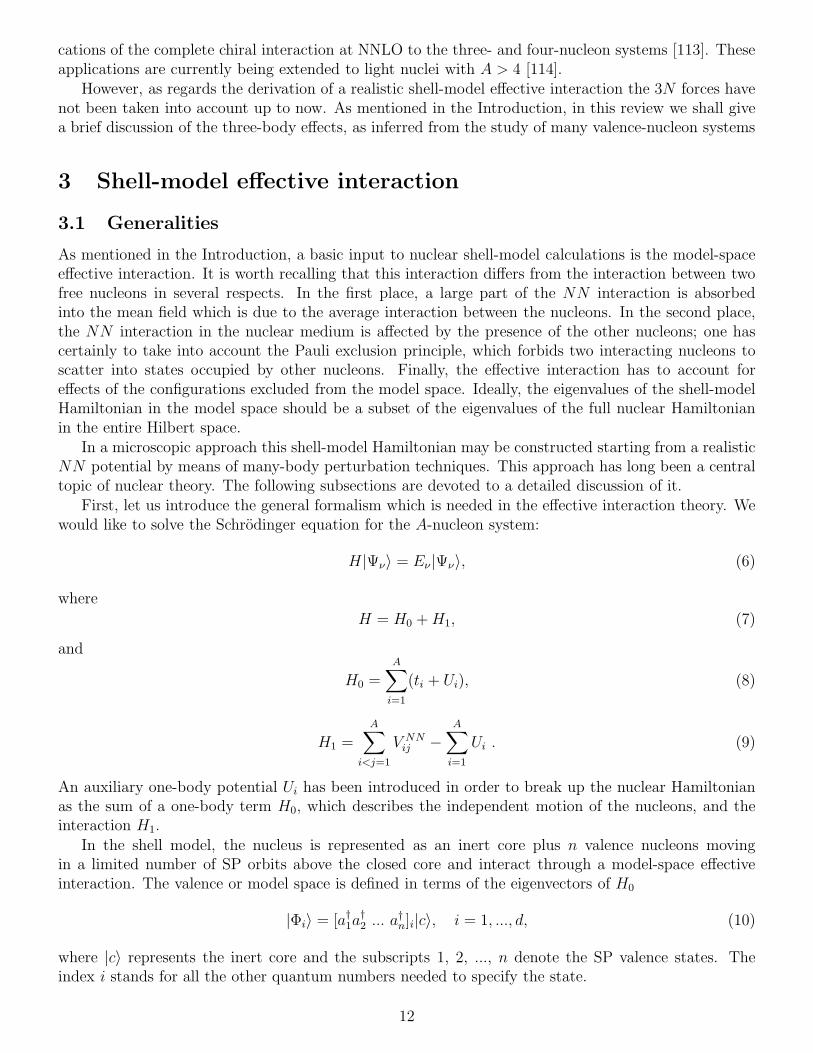
The action of the time-development operator on the unperturbed wave function |Φi〉 may be representedby an infinite collection of diagrams. The type of diagrams we consider here is referred to as time-orderedGoldstone diagrams (for a description of Goldstone diagrams see for instance Ref. [117])
As an example, we show in Fig. 1 a second-order time-ordered Goldstone diagram , which is oneof the diagrams appearing in (25). The dashed vertex lines denote VNN -interactions (for the sake ofsimplicity we take H1 = VNN), a and b represent two passive particle states while 1, 2, 3, and 4 arevalence states. From now on in the present section, the passive particle states will be represented byletters and dashed-dotted lines.
1 2
3 4
a b
A
Fig. 1: A second-order time-ordered Goldstone diagram.
The diagram A of Fig. 1 gives a contribution
A = a†aa†b|c〉 ×
1
4Vab34V3412I(A), (26)
where Vαβγδ are non-antisymmetrized matrix elements of VNN . I(A) is the time integral
I(A) = limǫ→0+
limt′→−∞(1−iǫ)
(−i)2∫ 0
t′dt1
∫ t1
t′dt2e
−i(ǫ3+ǫ4−ǫa−ǫb)t1 e−i(ǫ1+ǫ2−ǫ3−ǫ4)t2 , (27)
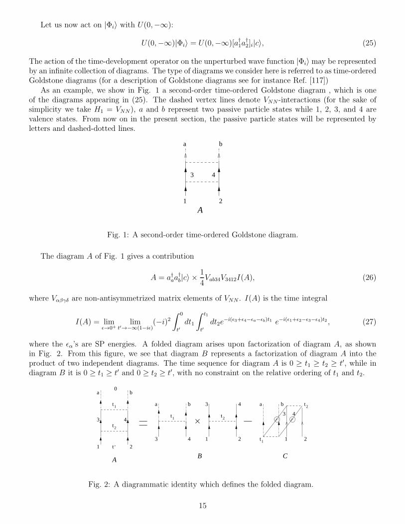
where the ǫα’s are SP energies. A folded diagram arises upon factorization of diagram A, as shownin Fig. 2. From this figure, we see that diagram B represents a factorization of diagram A into theproduct of two independent diagrams. The time sequence for diagram A is 0 ≥ t1 ≥ t2 ≥ t′, while indiagram B it is 0 ≥ t1 ≥ t′ and 0 ≥ t2 ≥ t′, with no constraint on the relative ordering of t1 and t2.
0
t
t1
2
t t
t
1 2
1
1 2
3 4
a b
a b
3 4
3 4
1 2
a b t2
3 4
1 2
’t
AB C
Fig. 2: A diagrammatic identity which defines the folded diagram.
15

Therefore, diagrams A and B are not equal, unless subtracting from B the time-incorrect contributionrepresented by the folded diagram C. It is worth noting that lines 3 and 4 in C are not hole lines, butfolded active particle lines. From now on the folded lines will be denoted by drawing a little circle.Explicitly, diagram C is given by
C = a†aa†b|c〉 ×
1
4Vab34V3412I(C), (28)
where
I(C) = limǫ→0+
limt′→−∞(1−iǫ)
(−i)2∫ 0
t′dt1
∫ 0
t1
dt2e−i(ǫ3+ǫ4−ǫa−ǫb)t1 e−i(ǫ1+ǫ2−ǫ3−ǫ4)t2 . (29)
Note that the rules to evaluate the folded diagrams are identical to those for standard Goldstonediagrams, except counting as hole lines the folded active lines in the energy denominator.
We now introduce the concept of generalized folded diagram and derive a convenient method tocompute it in a degenerate model space. Let us consider, for example, the diagrams shown in Fig. 3.All the three diagrams A, B, and C have identical integrands and constant factors, the only differencebeing in the integration limits. The integration limits of diagram A correspond to the time ordering0 ≥ t1 ≥ t2 ≥ t3 ≥ t4 ≥ t′. As pointed out before, the factorization of A into two independent diagrams(diagram B) violates the above time ordering. To correct for the time ordering in B, one has to subtractthe folded diagram C, whose time constraints are 0 ≥ t1 ≥ t2 ≥ t′, 0 ≥ t3 ≥ t4 ≥ t′, and t3 ≥ t2. Fivedifferent time sequences satisfy the above three constraints, thus C consists of five ordinary foldeddiagrams (see Fig. 4) and is called generalized folded diagram. From now on the integral sign willdenote the generalized folding operation.
1 2
t
t
t
t4
3
2
1
t
t
1
2 t t t
t t t
4
3
2
1
4
3
t1 > t > t > t2 3 4
a b
c d
3 4
t > t , t > t1 2 3 4 t > t , t > t , t > t1 2 3 4 3 2
3 4
c d
1 2
3 4
a b
3 4
c d
1 2
3 4
a b
e f
e f e f
AB C
Fig. 3: A diagrammatic identity which illustrates the generalized folded diagram.
An advantageous method to evaluate generalized folded diagrams in a degenerate model space isas follows. Let us consider diagram C of Fig. 3. As pointed out before, A, B, and C have identicalintegrands and constant factors, so that we may write the time integral I(C) as ([38], pp. 16-18)
I(C) = I(B)− I(A) =1
ǫ1 + ǫ2 − ǫ3 − ǫ4
[
1
(ǫ3 + ǫ4 − ǫe − ǫf )(ǫ3 + ǫ4 − ǫc − ǫd)(30)
− 1
(ǫ1 + ǫ2 − ǫe − ǫf )(ǫ1 + ǫ2 − ǫc − ǫd)
]
1
ǫ1 + ǫ2 − ǫa − ǫb.
16

In a degenerate model space, the first factor is infinite, while the second is zero. However, I(C) canbe determined by a limiting procedure. If we write ǫ1 + ǫ2 = ǫ3 + ǫ4 + ∆, where ∆ → 0, we can putEq. (31) into the form
I(C) = lim∆→0
1
∆
[
1
(ǫ3 + ǫ4 − ǫe − ǫf)(ǫ3 + ǫ4 − ǫc − ǫd)− 1
(ǫ3 + ǫ4 − ǫe − ǫf +∆)(ǫ3 + ǫ4 − ǫc − ǫd +∆)
]
(31)
× 1
(ǫ3 + ǫ4 − ǫa − ǫb +∆)
=
[
1
(ǫ3 + ǫ4 − ǫe − ǫf )2(ǫ3 + ǫ4 − ǫc − ǫd)+
1
(ǫ3 + ǫ4 − ǫe − ǫf )(ǫ3 + ǫ4 − ǫc − ǫd)2
]
× 1
(ǫ3 + ǫ4 − ǫa − ǫb).
Thus, the energy denominator of the generalized folded diagram C can be expressed as the derivative ofthe energy denominator of the l.h. part of the diagram with respect to the energy variable ω, calculatedat ǫ1 + ǫ2:
I(C) = − 1
ǫ3 + ǫ4 − ǫa − ǫb
d
dω
(
1
ω − ǫc − ǫd
1
ω − ǫe − ǫf
)
ω=ǫ1+ǫ2
. (32)
The last equation will prove to be very useful to evaluate the folded diagrams.
t
t t
t
3 4
c d a b
3 4
1 2
t
t
t
tt
t
t
t
t
t
t
t
t
t t
t
t
t
t
t
cd
a
b
cd
a
b
cd a b
c d
a b
c da
b
1 2
34
1 2
34
1 2
34
3 4
1 2 1 2
34
1
2
3
4
1
2
3
41
2
3
4
1
2
3
4
1
2
3
4
1
2
3
4
t > t t > t t > t1 3 4 3 22 , , t > t > t > t3 4 t > t > t > t3 1 4 2
t > t > t > t t > t > t > t t > t > t > t3 1 2 4 1 3 2 4 1 3 4 2
e f
e f e f
e f e f e f
21
Fig. 4: Generalized folded diagram expressed as sum of ordinary folded diagrams.
3.2.2 The decomposition theorem
Let us consider again the wave function U(0,−∞)|Φi〉. We can rewrite it as
U(0,−∞)|Φi〉 = UL(0,−∞)|Φi〉 × U(0,−∞)|c〉, (33)
where the subscript L indicates that all the H1 vertices in UL(0,−∞)|Φi〉 are valence linked, i.e. arelinked directly or indirectly to at least one of the valence lines. We now factorize each of the two termson the r.h.s. of Eq. (33) in order to write U(0,−∞)|Φi〉 in a form useful for the derivation of themodel-space secular equation.
17

. . .1C||C )0,(QU
. . .
t 0
t
C|C|)0,(QU
Fig. 5: Diagrammatic representation of UQ(0,−∞)|c〉 and 〈c|U(0,−∞)|c〉.
We first consider U(0,−∞)|c〉, which can rewritten as
U(0,−∞)|c〉 = UQ(0,−∞)|c〉 × 〈c|U(0,−∞)|c〉, (34)
where UQ(0,−∞)|c〉 denotes the collection of diagrams in which every vertex is connected to the timet = 0 boundary. In fact, UQ(0,−∞)|c〉 is proportional to the true ground-state wave function of theclosed-shell system, while 〈c|U(0,−∞)|c〉 represents all the vacuum fluctuation diagrams. These twoterms are illustrated in the first and second line of Fig. 5, respectively.
A similar factorization of UL(0,−∞)|Φi〉 can be performed, which can be expressed in terms of theso-called Q-boxes. The Q-box, which should not be confused with the projection operator Q introducedin Sec. 3.1, is defined as the sum of all diagrams that have at least one H1-vertex, are valence linked andirreducible (i.e., with at least one passive line between two successive vertices). Clearly, UL(0,−∞)|Φi〉must terminate either in an active or passive state at t = 0, thus we can write
UL(0,−∞)|Φi〉 = |χPi 〉+ |χQ
i 〉, (35)
as shown in Fig. 6. Note that in this figure the intermediate indices k, a, ... represent summations overall P -space states.
. . .
. . .
UL(0, ) | Φ QQ
Q
Q
nn
a
i ii
i i
j jj
j=1
d
n>d
ik
Fig. 6: Diagrammatic representation of UL(0,−∞)|Φi〉.
It is also possible to factorize out of |χQi 〉 a term belonging to |χP
i 〉 by means of the folded-diagramfactorization. In Fig. 7 we show, as an example, how a 2-Q-box sequence can be factorized.
It is worth noting the similarity between Fig. 7 and Fig. 3. As a matter of fact, when factorizingdiagram A time incorrect contributions arise in diagram B, that are compensated by subtracting fromit the generalized folded diagram C.
Using the generalized folding procedure, we are able to factorize out of each term in |χQi 〉 a diagram
belonging to |χPi 〉 (see Fig. 8). Applying this factorization to all the terms in |χQ
i 〉, collecting columnwisethe diagrams on the r.h.s. in Fig. 8 and adding them up, we may represent |χQ
i 〉 as shown in Fig. 9.
18

k
n
jt
Q
Q
A
Q
n
t
tQ
jk
k
t
t
B
Q
k
n
t
tQ
k
j
C
t
t
2
13
42
1
4
3
t
tt
t4
3
2
1
0t
Fig. 7: Factorization of a 2-Q-box sequence.
The collection of diagrams in the upper parenthesis of Fig. 9 is simply 〈Φj |UL(0,−∞)|Φi〉, which,according to Eq. (35), is related to |χP
i 〉 by
|χPi 〉 =
d∑
j=1
|Φj〉〈Φj|UL(0,−∞)|Φi〉 . (36)
Therefore, taking into account Figs. 6 and 9, and Eq. (36) we can express UL(0,−∞)|Φi〉 as
UL(0,−∞)|Φi〉 =d
∑
j=1
UQL(0,−∞)|Φj〉〈Φj |UL(0,−∞)|Φi〉, (37)
where we have represented diagrammatically UQL(0,−∞)|Φj〉 in Fig. 10.
Q
n
i
n
j
Q
j
i
n
j
i
Q
Q
n
j
Q
j
i
Q Q
n
j
Q
j
k
k
i
i
j
kn
k
n k j
k j i
QQQQ
Q
Q
Q
n k j
k j l
Q Q Q
i
l
n
Q
k
j
Q
i
. . .
Fig. 8: Factorization of |χQi 〉 using the generalized folding procedure.
19

Eqs. (33), (34), and (37) define the decomposition theorem, which we rewrite as follows:
U(0,−∞)|Φi〉 =d
∑
j=1
UQ(0,−∞)|Φj〉〈Φj |U(0,−∞)|Φi〉, (38)
where
〈Φj |U(0,−∞)|Φi〉 = 〈Φj|UL(0,−∞)|Φi〉 × 〈c|U(0,−∞)|c〉, (39)
and
UQ(0,−∞)|Φj〉 = UQL(0,−∞)|Φj〉 × UQ(0,−∞)|c〉 . (40)
χiQ
i
j
Q
i
jQ
Q
j
i
k . . .
n
j
Q Q
k
n
Q
k
j
Q
n
l
Q Q . . .
l
k
k
j
Fig. 9: |χQi 〉 wave function.
The decomposition theorem, as given by Eq. (38), states that the action of U(0,−∞) on |Φi〉 canbe represented as the sum of the wave functions UQ(0,−∞)|Φj〉 weighted with the matrix elements〈Φj|U(0,−∞)|Φi〉. Eq. (38) will play a crucial role in the next Sec. 3.2.3, where we shall give anexpression for the shell-model effective Hamiltonian.
t 0
t
Q
j
j
n
j
Q
n
k
Q
k
j
Q
n
l
Q
k
l
Q
k
j
. . .
Fig. 10: Diagrammatic representation of UQL(0,−∞)|Φj〉.
3.2.3 The model-space secular equation
For the sake of clarity, let us recall the model-space secular equation (11)
PHeffP |Ψα〉 = EαP |Ψα〉,
where α = 1, .., d, |Ψα〉 and Eα are the true eigenvectors and eigenvalues of the full Hamiltonian H .From now on, we shall use, for the convenience of the proof, the Schrodinger representation. However,
it is worth to point out that the results obtained hold equally well in the interaction picture.
20
First of all, we establish a one-to-one correspondence between some model-space parent states |ρα〉and d true eigenfunctions |Ψα〉. Let us start with a trial parent state
|ρ1〉 =1√d
d∑
i=1
|Φi〉, (41)
and act with the time development operator U(0,−∞) on it. More precisely, we construct the wavefunction
U(0,−∞)|ρ1〉〈ρ1|U(0,−∞)|ρ1〉
= limǫ→0+
limt′→−∞(1−iǫ)
eiHt′ |ρ1〉〈ρ1|eiHt′ |ρ1〉
. (42)
By inserting a complete set of eigenstates of H between the time evolution operator and |ρ1〉, we obtain
U(0,−∞)|ρ1〉〈ρ1|U(0,−∞)|ρ1〉
= limǫ→0+
limt′→−∞
∑
λ eiEλt
′
eEλǫt′ |Ψλ〉〈Ψλ|ρ1〉
∑
β eiEβt′eEβǫt′〈ρ1|Ψβ〉〈Ψβ|ρ1〉
=|Ψ1〉
〈ρ1|Ψ1〉≡ |Ψ1〉 . (43)
Here, |Ψ1〉 is the lowest eigenstate of H for which 〈Ψ1|ρ1〉 6= 0, this stems from the fact that the realexponential damping factor in the above equation suppresses all the other non-vanishing terms.
This procedure can be easily continued, thus obtaining a set of wave functions
|Ψα〉 =U(0,−∞)|ρα〉
〈ρα|U(0,−∞)|ρα〉, (44)
where〈ρα|ρα〉 = 1, (45)
〈ρα|Ψα〉 6= 0, (46)
〈ρα|Ψ1〉 = 〈ρα|Ψ2〉 = ... = 〈ρα|Ψα−1〉 = 0 . (47)
The above correspondence (Eqs. 44-47) holds if the parent states |ρα〉 are linearly independent. Underthis assumption, we can write
|ρα〉 =d
∑
i=1
Cαi |Φi〉, (48)
withd
∑
i=1
Cαi C
βi = δαβ . (49)
By construction, |Ψα〉 is an eigenstate of H , so, using Eq. (44), we can write
HU(0,−∞)|ρα〉
〈ρα|U(0,−∞)|ρα〉= Eα
U(0,−∞)|ρα〉〈ρα|U(0,−∞)|ρα〉
. (50)
Now, making use of Eq. (48) and applying the decomposition theorem as expressed by Eq. (38), theabove equation becomes
H
∑
ij UQ(0,−∞)|Φj〉〈Φj |U(0,−∞)|Φi〉Cαi
∑
km〈Φk|U(0,−∞)|Φm〉CαkC
αm
= Eα
∑
ij UQ(0,−∞)|Φj〉〈Φj|U(0,−∞)|Φi〉Cαi
∑
km〈Φk|U(0,−∞)|Φm〉CαkC
αm
. (51)
In order to simplify the above expression, we define the coefficients bαj
bαj =
∑
i〈Φj |U(0,−∞)|Φi〉Cαi
∑
km〈Φk|U(0,−∞)|Φm〉CαkC
αm
=
∑
i〈Φj |UL(0,−∞)|Φi〉Cαi
∑
km〈Φk|UL(0,−∞)|Φm〉CαkC
αm
, (52)
21

where the r.h.s. of the above equation has been obtained by use of Eq. (39), which cancels out thevacuum fluctuations diagrams 〈c|U(0,−∞)|c〉 of Fig. 5. Multiplying Eq. (51) by 〈Φk|, it becomes
d∑
j=1
〈Φk|HUQ(0,−∞)|Φj〉bαj = Eαbαk , (53)
where use has been made of the relation 〈Φk|UQ(0,−∞)|Φj〉 = δkj (see Ref. [121]). The above equationis the model-space secular equation we needed, where Heff is given by HUQ(0,−∞) and bαj represents
the projection of |Ψα〉 onto the model-space wave function |Φj〉.
Ec Ec
0. . .
Fig. 11: Goldstone linked-diagram expansion of Ec−E0c . The cross insertions represent the H0 operator.
In Eq. (53) we can write the Hamiltonian H as H = H0+H1. First, let us consider the contributionfrom H0. Since |Φi〉 is an eigenstate of H0 and 〈Φi|UQ(0,−∞)|Φj〉 = δij , we obtain
〈Φi|H0UQ(0,−∞)|Φj〉 = 〈Φi|H0|Φj〉 = δij(E0c + E0
v), (54)
where E0c is the unperturbed core energy and E0
v is the unperturbed energy of the two valence nucleonswith respect to E0
c .As for the matrix element 〈Φi|H1UQ(0,−∞)|Φj〉, we see from inspection of Eq. (40) that it contains
a collection of diagrams in which H1 is not linked to any valence line at t = 0. These diagramsare obtained acting with H1 on UQ(0,−∞)|c〉 and their contribution to the l.h.s. of Eq. (53) isδij〈c|H1UQ(0,−∞)|c〉 = δij(Ec −E0
c ), Ec being the true ground-state energy of the closed-shell system.The diagram expansion of (Ec −E0
c ) is given in Fig. 11 as illustrated in [122].The other terms of 〈Φi|H1UQ(0,−∞)|Φj〉 are all linked to the external active lines. By denoting,
for simplicity, the collection of these terms as
〈Φi|[H1UQ(0,−∞)]L|Φj〉, (55)
the secular equation (53) can be rewritten in the following form:
E0v +
d∑
j=1
〈Φi|[H1UQ(0,−∞)]L|Φj〉bαj = (Eα − Ec)bαi . (56)
We now define
H1eff = [H1UQ(0,−∞)]L, (57)
and show in Fig. 12 a diagrammatic representation of its matrix elements, which has been obtainedstarting from the definition of UQL(0,−∞)|Φj〉 given in Fig. 10. It should be noted that we have two
kinds of Q-box, Q and Q′. Q and Q′ are a collection of irreducible, valence-linked diagrams with atleast one and two H1-vertices, respectively. The fact that the lowest order term in Q′ is of second orderin H1 is just because of the presence of H1 in the matrix elements of Eq. (55).
Formally, H1eff can be written in operator form as
H1eff = Q− Q′
∫
Q+ Q′
∫
Q
∫
Q− Q′
∫
Q
∫
Q
∫
Q+ ... , (58)
22

where the integral sign represents a generalized folding operation. It is worth noting that, by definition,the Q-box contains diagrams at any order in H1. Actually, when performing realistic shell-modelcalculations it is customary to include diagrams up to a finite order in H1. A complete list of all theQ-box diagrams up to third order can be found in Ref. [45].
. . .QHeff
j j j
k
k j k
kl
l
QQQQQ
i i i i
Fig. 12: Diagrammatic representation of Heff matrix elements.
The Schrodinger equation (6) is finally reduced to the model-space eigenvalue problem of Eq. (56),whose eigenvalues are the energies of the A-nucleus relative to the core ground-state energy Ec. Asmentioned above, the latter can be calculated by way of the Goldstone expansion [122], expressed asthe sum of diagrams shown in Fig. 11. It is also worth noting that the operator H1
eff , as defined byEq. (58), contains both one- and two-body contributions since in our derivation of the of Eq. (56) we haveconsidered nuclei with two-valence nucleons. All the one-body contributions, the so-called S-box [123],once summed to the eigenvalues of H0, E
0v , give the SP term of the effective shell-model Hamiltonian.
The eigenvalues of this term represent the energies of the nucleus with one-valence nucleon relative tothe core. This identification justifies the commonly used subtraction procedure [123] where only thetwo-body terms of H1
eff (the effective two-body interaction Veff) are retained while the single-particleenergies are taken from experiment.
In this context, it is worth to mentioning that in some recent papers [124, 125] the SP energies andthe two-body interaction employed in realistic shell-model calculations are derived consistently in theframework of the linked-cluster expansion. In particular, in Ref. [124], where the light p-shell nuclei havebeen studied using the CD-Bonn potential renormalized through the Vlow−k procedure (see Sec. 4.2),a Hartree-Fock basis is derived which is used to calculate the binding energy of 4He and the effectiveshell-model Hamiltonian composed of one- and two-body terms.
In concluding this brief discussion of Eq. (56), it is worth to point out that for systems with more thantwo valence nucleons H1
eff contains 1-, 2-, 3-,· · · , n-body components, even if the original Hamiltonianof Eq. (7) contains only a two-body force [126]. The role of these effective many-body forces as well asthat of a genuine 3-body potential in the shell model is still an open problem (see [127] and referencestherein) and is outside the scope of this review. However, we shall come back to this point in Sec. 5.3.4.
In Sec. 3.2.1 we have shown how, in a degenerate model space, a generalized folding diagram can beevaluated. In [128], it has been shown that a term like −Q′
∫
Q may be written as
− Q′
∫
Q =dQ′(ω)
dωQ(ω), (59)
where ω is equal to the energy of the incoming particles.
The above result may be extended to obtain a convenient prescription to calculate H1eff as given by
Eq. (58). We can write
H1eff =
∞∑
i=0
Fi , (60)
23

where
F0 = Q,
F1 = Q1Q,
F2 = Q2QQ+ Q1Q1Q, (61)
...
and
Qm =1
m!
dmQ(ω)
dωm
∣
∣
∣
∣
ω=ω0
, (62)
ω0 being the energy of the incoming particles at t = −∞.Note that in Eq. (61) we have made use of the fact that, by definition,
dQ′(ω)
dω=dQ(ω)
dω. (63)
The number of terms in Fi grows dramatically with i. Two iteration methods to partially sum upthe folded diagram series have been introduced in Refs. [37, 129, 130]. These methods are known as theKrenciglowa-Kuo (KK) and the Lee-Suzuki (LS) procedure, respectively. In [130], it has been shownthat, when converging, the KK partial summation converges to those states with the largest modelspace overlap, while the LS one converges to the lowest states in energy.
The LS iteration procedure was proposed within the framework of an approach to the construction ofthe effective interaction known as Lee-Suzuki method, which is based on the similarity transformationtheory. In the following subsection we shall briefly present this method to illustate the LS iterativetechnique used to sum up the folded-diagram series (60).
3.3 The Lee-Suzuki method
Let us start with the Schrodinger equation for the A-nucleon system as given in Eq. (6) and considerthe similarity transformation
H = X−1HX, (64)
where X is a transformation operator defined in the whole Hilbert space.If we require that
QHP = 0, (65)
then it can be easily proved that the P -space effective Hamiltonian satisfying Eq. (11) is just PHP .Equation (65) is the so-called decoupling equation, whose solution leads to the determination of Heff .
There is, of course, more than one choice for the transformation operator X . We take
X = eΩ, (66)
where the wave operator Ω satifies the conditions:
Ω = QΩP, (67)
PΩP = QΩQ = PΩQ = 0 . (68)
Taking into account Eq. (67), we can write X = 1 + Ω and consequently
Heff = PHP = PHP + PH1QΩ, (69)
24

with H1 defined in Eq. (9), while the decoupling equation (65) becomes
QH1P +QHQΩ− ΩPHP − ΩPH1QΩ = 0 . (70)
We now introduce the P -space effective interaction R by subtracting the unperturbed energy PH0Pfrom Heff :
R = PH1P + PH1QΩ . (71)
In a degenerate model space PH0P = ω0P , we can consider a linearized iterative equation for thesolution of the decoupling equation (70)
[E0 − (QHQ− Ωn−1PH1Q)]Ωn = QH1P − Ωn−1PH1P . (72)
We now write the Q-box introduced in Sec. 3.2.2 in operatorial form as given in [130]
Q = PH1P + PH1Q1
E0 −QHQQH1P, (73)
and define Rn as the n-th order iterative effective interaction
Rn = PH1P + PH1QΩn . (74)
Then, if we start with Ω0 = 0 in Eq. (72), Rn can be written in terms of the Q-box and itsderivatives:
R1 = Q,
R2 = [1− Q1]−1Q,
R3 = [1− Q1 − Q2R2]−1Q,
...
Rn =
[
1− Q1 −n−1∑
m=2
Qm
n−1∏
k=n−m+1
Rk
]−1
Q (75)
where Qn is defined in Eq. (62).The solution Rn so obtained corresponds to a certain resummation of the folded diagrams to infinite
order. In fact, if we consider, for example, R2 and expand it in power series of Q1, we obtain
R2 = [1− Q1]−1Q = 1 + Q1Q + Q1Q1Q + ... (76)
It is clear from the above expression that R2 contains terms corresponding to an infinite number offolds.
It can be shown that the Lee-Suzuki method yields converged results after a small number ofiterations [123], making this procedure very advantageous to sum up the folded-diagram series.
4 Handling the short-range repulsion of the NN potential
As already pointed out, a most important goal of nuclear shell-model theory is to derive the effectiveinteraction between valence nucleons directly from the free NN potential. In Sec. 3, we have shownhow this effective interaction may be calculated microscopically within the framework of a many-bodytheory. As is well known, however, VNN is not suitable for this kind of approach. In fact, owing to thecontribution from the repulsive core, the matrix elements of VNN are generally very large and an order-by-order perturbative calculation of the effective interaction in terms of VNN is clearly not meaningful.
25

Ψ
r0
VNN
Φ
Fig. 13: (Color online) Radial dependence of the relative wave function Ψ of two nucleons interactingvia a hard-core potential VNN . Φ refers to the uncorrelated wave function.
A resummation method has to be employed in order to take care of the strong short-range repulsioncontained in VNN .
This point is more evident if we consider the extreme model of a hard-core potential, as is the caseof the potential models developed in the early 1960s. This situation is illustrated in Fig. 13. For thesepotentials the perturbation expansion of the effective interaction in terms of VNN is meaningless, sinceeach term of the series involving matrix elements of the NN potential between unperturbed two-bodystates is infinite. This is because the unperturbed wave function, in contrast to the true wave function,gives a non-zero probability of finding a particle located inside the hard-core distance.
The traditional way out of this problem is the so-called Brueckner reaction matrix G, which is basedon the idea of treating exactly the interaction between a given pair of nucleons [131]. The G matrix,defined as a sum of all ladder-type interactions (see Sec. 4.1.2), is used to replace the NN interactionvertices once a rearrangement of the effective interaction perturbative series has been performed.
Recently, a new method to renormalize the NN interaction has been proposed [42, 43]. A low-momentum model space defined up to a cutoff momentum Λ is introduced and an effective potentialVlow−k is derived from VNN . This Vlow−k satisfies a decoupling condition between the low- and high-momentum spaces. Moreover, it is a smooth potential which preserves exactly the on-shell propertiesof the original potential and it is thus suitable to advantageously replace VNN in realistic many-bodycalculations.
Secs. 4.1 and 4.2 are devoted to the description of the reaction G matrix and Vlow−k potential,respectively.
Before doing this, however, it may be worth recalling that a method to avoid the G-matrix treatmentto eliminate effects of the repulsive core in the NN potential was proposed in the late 1960s [132, 40].As already mentioned in the Introduction, this consists in using the experimental NN phase shifts todeduce matrix elements of the NN potential in a basis of relative harmonic oscillator states. Thesematrix elements, which have become known as the Sussex matrix elements (SME), have been usedin several nuclear structure calculations, but the agreement with experiment has been generally onlysemi-quantitative. A comparison between the results obtained by Sinatkas et al. [133] using the SMEand those obtained with a realistic effective interaction derived from the Bonn A potential is made forthe N=50 isotones in [134].
4.1 The Brueckner G-matrix approach
4.1.1 Historical introduction
The concept of G matrix originates from the theory of multiple scattering of Watson [135, 136]. In thisapproach, the elastic scattering of a fast particle by a nucleus was described by way of a transformed
26
potential obtained in terms of the Lippmann-Schwinger matrix [137] for the two-body scattering. Theprocedure of Watson for constructing such an “equivalent two-body potential” was generalized to thestudy of nuclear many-body systems by Brueckner and co-workers [131, 138]. They introduced a reactionmatrix for the scattering of two nucleons while they are moving in the nuclear medium. This matrix,which is known as the Brueckner reaction matrix, includes all two-particle correlations via summing allladder-type interactions, and made it possible to perform Hartree-Fock self-consistent calculations fornuclear matter.
Only a few years later Goldstone [122] proved a new perturbation formula for the ground-state energyof nuclear matter which gave the formal basis of the Brueckner theory. The Goldstone linked-diagramtheory applies to systems with non-degenerate ground state, which is the case of nuclear matter as wellas of closed-shell finite nuclei.
The Brueckner theory was seen to be the key to solve the paradox on which the attention of manynuclear physicists was focused during the early 1950s. In fact, it allowed to reconcile a description ofthe nucleus in terms of an overall potential and the peculiar features of the two-body nuclear force.This was very well evidenced in the paper by Bethe [139], whose main purpose was indeed to establishthat the Brueckner theory provided the theoretical foundation for the shell model.
After their first works, Brueckner and co-workers published a series of papers on the same subject[140, 141, 142, 143, 144], where further analyses and developments of the method as well as numericalcalculations were given. Important advances as regards nuclear matter were provided by the work ofBethe and Goldstone [145] and Bethe et al. [146]. For several years up to the 1960s, nuclear physicistswere indeed very active in this field, as may be seen from the review papers by Day [147], Rajaramanand Bethe [148], and Baranger [149], where comprehensive lists of references can be found. For a recentreview of the developments in this area made Bethe and coworkers we refer to [150].
As regards open-shell nuclei, we have shown in the previous section that the model-space effectiveinteraction may be obtained by way of a linked-diagram expansion containing both folded and non-folded Goldstone diagrams. An order-by-order perturbative calculation of such diagrams in terms ofVNN is not appropriate and one has to resort again to the reaction matrix G.
The renormalization of VNN through the Brueckner theory has been the standard procedure to deriverealistic effective interactions since the pioneering works of the early 1960s. A survey of shell-modelcalculations employing the G matrix is given in Secs. 5.1 and 5.2.
In Sec. 4.1.2 we shall define the reaction matrix G and discuss the main problems related to itsdefinition. Then, in Sec. 4.1.3, we shall address the problem of how the reaction matrix may becalculated, focusing attention on the GT matrix for which plane waves are used as intermediate states.It is, in fact, this matrix which is most commonly used nowadays in realistic shell-model calculations.For simplicity, almost everywhere in this section we shall denote the NN potential by V .
4.1.2 Essentials of the theory
In the literature, the G matrix is typically introduced by way of the Goldstone expansion for thecalculation of the ground-state energy in nuclear matter and closed shell nuclei. As a first step, theground-state energy is written as a linked-cluster perturbation series. Then, all diagrams differingone from another only in the number of V interactions between two particles lines are summed. Thiscorresponds to define a well-behaved two-body operator, the reaction matrix G, that replaces thepotential V in the series. A very clear and simple presentation of the G matrix along this line isprovided in the paper by Day [147].
Here, we shall not discuss the details of the G-matrix theory, but simply give the elements neededto make clear its definition in connection with the derivation of the model-space effective interactionfor open-shell nuclei. Therefore, in the following we refer, as in the previous section, to an A-nucleonsystem with the Hamiltonian given by Eqs. (7)-(9) and represented as a doubly closed core plus valence
27

nucleons moving in a limited number of SP orbits above the core.The two-body operator G is defined by the integral equation
G(ω) = V + VQ2p
ω −H0
G(ω), (77)
where ω is an energy variable known as “starting energy” and Q2p an operator which projects ontoparticle-particle states, namely states composed of two SP levels above the doubly closed core. As weshall discuss later, this operator may be chosen in different ways depending on the specific context inwhich it is used. Here it is worth noting that its presence in Eq. (77) reminds us that the G matrix,differently from the Lippmann-Schwinger T matrix, is defined in the nuclear medium. It may be alsonoted that the starting energy ω is not a free parameter. Rather, its value is determined by the physicalproblem being studied. For the T matrix, ω denotes the scattering energy for two particles in free space,but depends on the nuclear medium for the G matrix. In fact, we shall see that for a G matrix to beused within the linked-diagram expansion of the effective interaction ω depends on the diagram whereG appears. Only in some cases it represents the energy of the two-particle incoming state, which wasinstead the meaning of the energy variable ω used in Sec. 3.
Let us start by writing the Q2p operator as
Q2p =∑
ij
C(ij)|φij〉〈φij|, (78)
where the state |φij〉, which is the antisymmetrized product of the two SP states |i〉 and |j〉, is aneigenstate of H0 with energy ǫi + ǫj . The constant C(ij) is 1 if the state |φij〉 pertains to the spacedefined by Q2p, 0 otherwise. We now introduce the operator P2p which projects on the complementaryspace
P2p = 1−Q2p. (79)
Taking matrix elements of G between states of the P2p-space we have
〈φkl|G(ω)|φnm〉 = 〈φkl|V |φnm〉+∑
ij
〈φkl|V |φij〉C(ij)
ω − ǫi − ǫj〈φij|G(ω)|φnm〉, (80)
which in a series expansion form becomes
〈φkl|G(ω)|φnm〉 = 〈φkl|V |φnm〉+∑
ij
〈φkl|V |φij〉C(ij)
ω − ǫi − ǫj〈φij|V |φnm〉
+∑
iji′j′
〈φkl|V |φij〉C(ij)
ω − ǫi − ǫj〈φij|V |φi′j′〉
C(i′j′)
ω − ǫi′ − ǫj′〈φi′j′|V |φnm〉+ · · · (81)
The above expansion can be represented diagrammatically by the series shown in Fig. 14. Thediagrams on the r.h.s. of this figure are known as “ladder” diagrams and each diagram corresponds toa situation in which a pair of particles interacts a certain number of times with the restriction that theintermediate states involved in the scattering must be those defined through the Q2p operator. In otherwords, two particles initially in a state of the P2p-space undergo a sequence of scatterings into states ofthe Q2p-space and then after several such scatterings go back to a state of the original space.
For the sake of completeness, we introduce the correlated wave function |ψnm(ω)〉 [145],
|ψnm(ω)〉 = |φnm〉+Q2p
ω −H0V |ψnm(ω)〉, (82)
28

= + + + ...
Fig. 14: Diagrammatic representation defining the matrix G.
which once iterated becomes
|ψnm(ω)〉 = |φnm〉+Q2p
ω −H0
G(ω)|φnm〉, (83)
where use has been made of the integral equation (77). Eq. (83) allows one to write the action of G onan unperturbed state as
G(ω)|φnm〉 = V |ψnm(ω)〉, (84)
which makes evident that the G operator may be considered an effective potential. The correlated wavefunction (82) and its properties are extensively discussed in Refs. [149, 151, 152].
At this point, we go further in our discussion clarifying the meaning of the starting energy ω andillustrating some possible choices of the projection operator Q2p.
Q
Q
2p =1
2p =0
n
n
n n
1
1
2
2
i
j
Fig. 15: A graph of the projection operator Q2p appropriate for open-shell nuclei.
Let us begin with Q2p. We define the Q2p operator by specifying its boundaries labelled by the threenumbers (n1,n2,n3), each representing a SP level, the levels being numbered starting from the bottomof the potential well. Explicitly, using Eq. (78) the operator Q2p is written as
C(ij) =
1 if i, j > n2
1 if n1 < i ≤ n2 and j > n2
or vice-versa0 otherwise.
The graph of Fig. (15) makes more clear its definition. Note that the index n3 denotes the numberof levels in the full space. In principle, it should be infinite; in practice, as we shall see in Sec. 4.1.3,it is chosen to be a large but finite number. As regards the indices n1 and n2, the only mandatoryrequiriment is that none of them should be below the last occupied orbit of the doubly closed core. Itis customary to take for n1 the number the SP levels below the Fermi surface while n2 may be chosenstarting from the last SP valence level and going up. How this choice is performed is better illustratedby an example.
Let us consider the nucleus 18O which in the shell-model framework is described as consisting of thedoubly closed 16O and two valence neutrons which are allowed to occupy the three levels of the sd shell.
29

The model-space effective interaction for 18O may be derived by using the linked-diagram expansion ofSec. 3, with the G matrix replacing the NN potential in all the irreducible, valence-linked diagramscomposing the Q-box. In so doing, one has to be careful to exclude from the Q-box those diagramscontaining a ladder sequence already included in the G matrix. We may take the matrix G with aQ2p operator as specified, for instance, by (3, 6,∞). In this case, one of two SP levels composing theintermediate state in the calculation of the G matrix has to be beyond the sd shell while the other onemay be also an sd level. Then, when calculating the Q-box the included diagrams strictly depend onthe considered G matrix. As an example, we have reported in Fig. 16 a first- and second-order diagramof the Q-box, the wavy lines denoting the G-interactions. As discussed in Sec. 3.2.2, the incoming andoutcoming lines of the A and B diagrams are levels of the sd shell, while the the intermediate state ofdiagram B should have at least one passive line. This means that none of the two SP states, x or y,could be a 0s or a 0p level and at least one of them must be beyond the sd shell. Therefore, if we takethe G matrix with the (3, 6,∞) Q2p operator, all possible B diagrams of Fig. 16 are already containedin the A diagram. On the other hand, if we increase the n2 using a G matrix with the (3, 10,∞)Q2p operator, the B diagrams should explicitly appear in the calculation of the Q-box providing thatx, y ≤ 10 and x and/or y ≥ 7. A detailed discussion on the points illustrated here is in Ref. [153].
x y
A B
k l k l
m n m n
Fig. 16: Second-order ladder diagram contained in the Q-box.
We now come to the energy variable ω which may be seen as the “starting energy” at which G iscomputed. We know that any G-vertex in a Q-box diagram is employed as the substitute for the ladderseries of Fig. 14 and therefore the corresponding starting energy depends on the diagram as a wholeand in particular on the location of the G-vertex in the diagram. For instance, the G matrices in thethree vertices of diagrams A and B of Fig. 16 have to be calcutated at ω = ǫk + ǫl, corresponding tothe energy of the two-particle incoming state. As an other example, we have shown in Fig. 17 thediagram A. To illustrate how ω is evaluated we have written it as the sum of the ladder sequence A1,A2,...,An,.... The lowest vertex of diagram A corresponds to 〈φmp|G(ω)|φkh〉 and its starting energy canbe determined by looking at the two lowest vertices in diagram A2 whose contribution may be writtenas
〈φmp|V |φxy〉〈φxy|V |φkh〉ǫk + ǫh − ǫx − ǫy
. (85)
Note that the energy denominator of the G matrix is given by ω−H0, H0 acting on the intermediatetwo-particle state |φxy〉. Therefore, to obtain the denominator of Eq. (85) as ω − ǫx − ǫy, one has tochoose ω = ǫk + ǫh. Similarly, for the upper G-vertex of diagram A ω = ǫk + ǫl + ǫh − ǫm. In both theprevious examples ω is different from the energy of the incoming state, which results to be ǫk + ǫl.
In concluding this subsection it is important to consider the dependence of the G matrix on theSP potential U , which explicitly appears in the denominator through H0. The advantages of differentchoices have been extensively investigated essentially in connection with the Goldstone expansion andits convergence properties (see the review paper by Baranger [149]).
30

= + + ...+ ... +
A A1 A2
p
h
p
h
p
h
p
h
m n
k l
yx
m n
k l
m n
k l
m
k l
n
Fig. 17: Illustration of the summation procedure to replace V vertices with G vertices.
It is worth recalling that, as a general rule, in a perturbation approach to nuclear structure calcu-lations one starts by summing and subtracting the SP potential U to the Hamiltonian so as to have asperturbation H1 = V − U . As a consequence, the diagrams of the Q-box for the shell-model effectiveinteraction contain −U as well as V vertices. Diagrams where −U vertices are attached to particle linesbetween successive V interactions may be taken into account directly through the reaction matrix. Thismeans that each diagram of the expansion shown in Fig. 14 is replaced with a new diagram in whichany number of −U insertions has been introduced in the particle lines. A typical diagram is shownin Fig. 18. In this way, a new reaction matrix may be introduced where the −U interactions for theintermediate particle states are summed up to all orders. More precisely, by changing the propagatorof the particle lines from H0 to H0 − Q2pUQ2p one obtains the reaction matrix with plane waves asintermediate states, which is usually called GT . Note that the term Q2pUQ2p instead of U is subtractedfrom H0 since, as pointed out in [149], particle and hole states are defined with respect to the SPpotential U . In other words, the Hamiltonian H0 −Q2pUQ2p, which commutes with Q2p, preserves theparticle and hole states as defined by U . The reaction matrix GT satisfies the integral equation
GT (ω) = V + V Q2p1
ω −Q2ptQ2pQ2pGT (ω), (86)
where one has to recall that t represents the kinetic energy.An extensive study of the properties and features of GT in the framework of the shell model can be
found in [153], where arguments in favor of the use of GT are given. We find it interesting to brieflyrecall these arguments here.
First of all, the GT matrix of Eq. (86) minimizes the dependence on the SP potential. In fact, itdepends only on Q2p while the reaction matrix G of Eq. (77) depends also on the spectrum of the SPstates of the Q2p space.
Fig. 18: Typical U insertions to the G-matrix intermediate states.
The second argument is essentially based on the paper by Bethe et al. [146], where it was shownthat all −U and Brueckner-Hartree-Fock self-energy insertions cancel each other when the self-energyis calculated on energy shell. This result may be plausibly extended [153] to low-energy intermediateparticle states not far off the energy shell, but such a cancellation is very unlikely for the high-energy
31

states. On the other hand, in nuclear matter calculations [152] it has been shown that the sum ofself-energy-insertion diagrams and other three-body clusters is almost negligible, in other words theytend to cancel each other. If we assume that this nuclear-matter result still holds for finite nuclei, wereasonably expect that only the −U insertions survive for high-energy intermediate states, so leadingto the reaction matrix GT . The use of the G matrix of Eq. (77) is instead suggested for low-lyingstates assuming that −U and Brueckner-Hartree-Fock self-energy insertions cancel approximately. Inother words the reaction matrix calculation may be performed following a two-step procedure, which isdiscussed in detail in [153]. Here we only give a sketch of such procedure.
Let us start by dividing the intermediate states of the Q2p space into high-energy and low-energystates, the Q2p operator being written as
Q2p = Qh2p +Ql
2p, (87)
with orthogonalized plane waves used for Qh2p and harmonic oscillator wave functions for Ql
2p. The fiststep consists in the calculation of the GT matrix of Eq. (86) with the projection operator taken as Qh
2p.Then using this reaction matrix instead of the NN potential the G matrix of Eq. (77) is calculatedwith a projection operator restricted to Ql
2p. Actually, the second step is carried out by means of a
pertubative expansion which implies that the final reaction matrix, which we call GT , is written as
GT (ω) = GT (ω) +GT (ω)Ql
2p
ω −H0GT (ω) +GT (ω)
Ql2p
ω −H0GT (ω)
Ql2p
ω −H0GT (ω) + · · · (88)
Hence GT is obtained by summing to GT the second -, third-, · · · order two-particle ladder diagrams withGT (ω) vertices and intermediate states restricted to the low-lying states defined by the Ql
2p operator.
These ladder terms may be directly included in the evaluation of the Q-box once the GT of Eq. (86) withQh
2p as projection operator has been calculated. Note that in so doing no −U or Brueckner-self-energy
insertions are explicitly included in the Q-box diagrams since, on the basis of the previous arguments,one may assume that they cancel each other.
It is worth to point out that no firm criteria exist on how to perform the partition of Eq. (87). Itis customary to take n2 in the definition of the Qh
2p operator so that it encompasses the shell above themodel space [153]. For example, if we consider again 18O we specify Q2p by (3, 10,∞) to define theGT matrix, then Ql
2p while corresponds to the 1p0f -shell and the ladder terms with two particle in this
shell are taken into account directly when the Q-box is evaluated.
4.1.3 Calculation of the reaction matrix
Starting from the introduction of the G matrix, several approximate techniques have been developedfor the solution of Eq. (77) A review of them together with a critical discussion can be found in[147, 149, 45, 154]. Among the early methods we would just like to mention the separation method ofMoszkowski and Scott [155] and the reference spectrum method of Bethe et al. [146], which have bothbeen extensively applied to both nuclear matter and finite nuclei. For many years, they were the primarymethods for G-matrix calculation and were first employed by Kuo and Brown [18] to calculate from theHamada-Johnston potential [63] the G matrix elements to be used in shell-model calculations for 18Oand 18F. It is interesting to note that during the 1970s significant advances were made in the calculationof the reaction matrix as regards the G matrix of Eq. (77) with harmonic oscillator intermediate statesas well as the GT matrix of Eq. (86) having plane-wave intermediate states. In fact, accurate solutionsof Eq. (77) were proposed by Barrett et al. [156] and of Eq. (86) by Tsai and Kuo [36], both of themproviding an exact treatment of the projection operator Q2p.
Here we shall only focus on the technique to compute the reaction matrix of Eq. (86), which we haveused in our shell-model calculations. More precisely, we shall describe the method proposed by Tsai
32

and Kuo [36], which was further investigated and applied by Krengiglowa et al. [153]. This method,based on a matrix inversion in the momentum space, allows, as mentioned above, an exact treatment ofthe projection Q2p operator except for the only approximation of using a finite value instead of infinityfor n3 defining Q2p.
Let us start by noting that a solution of Eq. (86) is
GT (ω) = V + V Q2p1
Q2p(e− V )Q2p
Q2pV, (89)
as it can be easily shown using the operator identity
1
A− B=
1
A+
1
AB
1
A−B, (90)
with e = ω − t, A = Q2p e Q2p, and B = Q2pV Q2p.The propagator of Eq. (89) was shown [36] to take the form
Q2p1
Q2p(e− V )Q2p
Q2p =1
e− V− 1
e− VP2p
1
P2p1
e−VP2p
P2p1
e− V, (91)
where P2p is defined in Eq. (79) . The identity (91) allows us to rewrite Eq. (89) as
GT (ω) = GTF (ω) + ∆G(ω), (92)
with
∆G(ω) = −V 1
e− VP2p
1
P2p1
e−VP2p
P2p1
e− VV (93)
and
GTF (ω) = V + V1
e− VV = V + V
1
eGTF (ω), (94)
where we have used the identity (90) with Q2p = 1 to obtain relation (94).An equivalent and very convenient expression of ∆G(ω) which has also the advantage to be applicable
when V is a hard-core potential is
∆G(ω) = −GTF (ω)1
eP2p
1
P2p[(1/e) + (1/e)GTF (1/e)]P2pP2p
1
eGTF (ω). (95)
The set of Eqs. (92, 94, 95) provides a very convenient way to calculate the GT matrix once afinite-n3 approximation is made, namely a truncated P2p-space is taken. Let us define
GR(ω) = GTF (1/e),
GL(ω) = (1/e)GTF ,
GLR(ω) = (1/e) + (1/e)GTF (1/e), (96)
then Eq. (92) in a matrix formalism can be written as
〈φkl|GT (ω)|φlm〉 = 〈φkl|GTF (ω)|φlm〉−∑
ijkl∈P2p
〈φkl|GL(ω)|φij〉× 〈φij|G−1LR(ω)|φkl〉〈k l|GR(ω)|φlm〉 . (97)
This equation makes clear the necessity of a finite-n3 approximation. In fact, the G−1LR matrix
appearing in this equation is defined in the P2p space and represents the inverse of the P2pGLRP2p
matrix, which has to be a finite matrix.
33

The basic ingredient for the calculation of the GT matrix through Eq. (92) is the matrix GTF whichis identical to the GT defined by Eq. (86), except that is free from the projection operator Q2p. Avery convenient way to calculate GTF (ω) is to employ the momentum-space matrix inversion method[157]. Once the GTF matrix elements in the momentum space are known, the matrices GL, GR, andGLR can be easily evaluated in the same space. As a final step, these matrices are all transformed inthe harmonic oscillator basis and the GT matrix is obtained by means of Eq. (97) though simple matrixoperations.
Here we have only given a sketch of the procedure to solve Eqs. (92), (94), (95). A detaileddescription of the whole procedure can be found in [153], where the validity of an n3-finite approximationis discussed. It is worth mentioning that this point is also discussed in Ref. [45].
4.2 The Vlow−k approach
In this subsection we shall describe in detail the derivation and main features of the low-momentum NNinteraction Vlow−k, which has been introduced in Refs. [42, 43, 44]. The idea underlying the constructionof Vlow−k from a realistic model for VNN is based on the renormalization group (RG) and the effectivefield theory (EFT) approaches [158, 92, 90, 91]. As mentioned in Sec. 2, while the high-quality NNpotentials all reproduce the empirical deuteron properties and low-energy phase shifts very accurately,they differ significantly from one another in the high momentum behavior. A cutoff momentum Λ thatseparates fast and slow modes is then introduced and from the original VNN an effective potential Vlow−k,satisfying a decoupling condition between the low- and high-momentum spaces, is derived by integratingout the high-momentum components. The main result is that Vlow−k is free from the model-dependenthigh-momentum modes. In consequence, it is a smooth potential which preserves exactly the onshellproperties of the original VNN , and is suitable to be used directly in nuclear structure calculations. InSec. 5.3.1, we will show that the Vlow−k approach provides a real alternative to the Brueckner G-matrixrenormalization procedure.
4.2.1 Derivation of the low-momentum NN potential 1 Vlow−k
In carrying out the above high-momentum integration, or decimation, an important requirement is thatthe low-energy physics of VNN is exactly preserved by Vlow−k. For the two-nucleon problem, there is onebound state, namely the deuteron. Thus one must require that the deuteron properties given by VNN
are preserved by Vlow−k. In the nuclear effective interaction theory, there are several well-developedmodel-space reduction methods. One of them is the Kuo-Lee-Ratcliff (KLR) folded diagram method[121, 38], which was originally formulated for discrete (bound state) problems. A detailed discussion ofthis method has been given earlier in Sec. 3.
For the two-nucleon problem, we want the effective interaction Vlow−k to preserve also the low-energyscattering phase shifts, in addition to the deuteron binding energy. Thus we need an effective interactionfor scattering (unbound) problems. A convenient framework for this purpose is the T -matrix equivalenceapproach, as described below.
We use a continuum model space specified by
P =
∫
dp | p〉〈p | , p ≤ Λ (98)
where p is the two-nucleon relative momentum and Λ the cutoff momentum which is also known as thedecimation momentum. Its typical value is about 2 fm−1 as we shall discuss later. Our purpose is tolook for an effective interaction PVeffP , with P defined above, which preserves certain properties of thefull-space interaction VNN for both bound and unbound states. This effective interaction is referred toas Vlow−k.
34

We start from the full-space half-on-shell T -matrix (written in a single partial wave channel)
T (k′, k, k2) = VNN (k′, k) + P
∫ ∞
0
q2dqVNN(k′, q)
1
k2 − q2T (q, k, k2). (99)
This is the T -matrix for the two-nucleon problem with the Hamiltonian
H = H0 + VNN = t+ VNN , (100)
t being the relative kinetic energy. We then define a P -space low-momentum T -matrix by
Tlow−k(p′, p, p2) = Vlow−k(p
′, p) + P∫ Λ
0
q2dqVlow−k(p′, q)
1
p2 − q2Tlow−k(q, p, p
2), (101)
where (p′, p) ≤ Λ and the integration interval is from 0 to Λ. In the above, the symbol P in front ofthe integration sign denotes principal value integration. We require the equivalence condition
T (p′, p, p2) = Tlow−k(p′, p, p2); (p′, p) ≤ Λ. (102)
The above equations define the effective low-momentum interaction; it is required to preserve the low-momentum (≤ Λ) half-on-shell T -matrix. Since phase shifts are given by the full-on-shell T -matrixT (p, p, p2), low-energy phase shifts given by the above Vlow−k are clearly the same as those of VNN .
In the following, let us show that a solution of the above equations may be found by way of the KLRfolded-diagram method [121, 38] described in Sec. 3 as a means to construct the shell-model effectiveinteraction. Within this approach the Vlow−k may be written in the operator form as
Vlow−k = Q− Q′
∫
Q + Q′
∫
Q
∫
Q− Q′
∫
Q
∫
Q
∫
Q+ ... , (103)
which contains a Q-box whose explicit definition is given below.In the time-dependent formulation, the T -matrix of Eq. (99) can be written as 〈k′ | V U(0,−∞) | k〉,
U(0,−∞) being the time-evolution operator. In this way a diagrammatic analysis of the T -matrix canbe made. A general term of T may be written as
〈k′ |[
V + V1
e(k2)V + V
1
e(k2)V
1
e(k2)V + ...
]
| k〉, (104)
where e(k2) ≡ (k2 −H0).Note that the intermediate states (represented by 1 in the numerator) cover the entire space. In
other words, we have 1 = P + Q where P denotes the model-space projection operator and Q itscomplement. Expanding it out in terms of P and Q, a typical term of T is of the form
VQ
eVQ
eVP
eVQ
eVP
eV. (105)
Let us now define the Q-box as
〈k′ | Q(k2) | k〉 = 〈k′ |[
V + VQ
e(k2)V + V
Q
e(k2)V
Q
e(k2)V + ...
]
| k〉, (106)
where all intermediate states belong to Q. One readily sees that the P -space portion of the T -matrixcan be regrouped in terms of a Q-box series, more explicitly as
〈p′ | T | p〉 = 〈p′ |[
Q + QP
e(p2)Q +Q
P
e(p2)Q
P
e(p2)Q + ...
]
| p〉. (107)
35
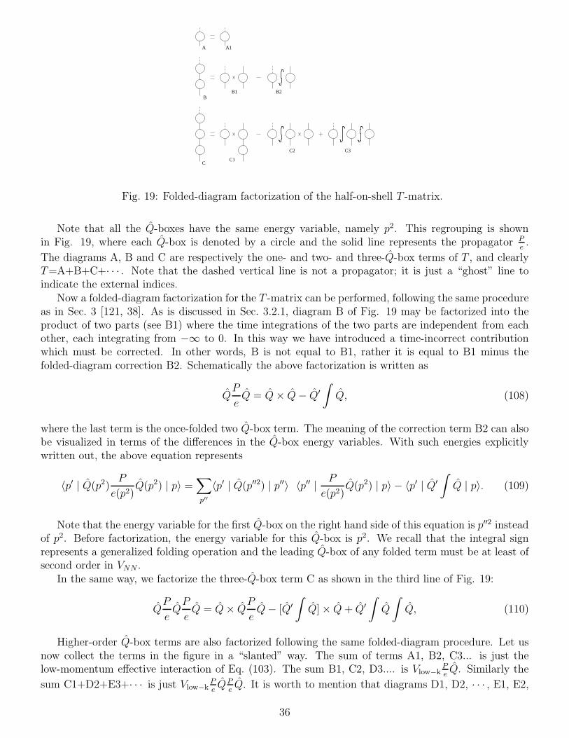
A A1
BB1 B2
CC1
C2 C3
Fig. 19: Folded-diagram factorization of the half-on-shell T -matrix.
Note that all the Q-boxes have the same energy variable, namely p2. This regrouping is shownin Fig. 19, where each Q-box is denoted by a circle and the solid line represents the propagator P
e.
The diagrams A, B and C are respectively the one- and two- and three-Q-box terms of T , and clearlyT=A+B+C+· · · . Note that the dashed vertical line is not a propagator; it is just a “ghost” line toindicate the external indices.
Now a folded-diagram factorization for the T -matrix can be performed, following the same procedureas in Sec. 3 [121, 38]. As is discussed in Sec. 3.2.1, diagram B of Fig. 19 may be factorized into theproduct of two parts (see B1) where the time integrations of the two parts are independent from eachother, each integrating from −∞ to 0. In this way we have introduced a time-incorrect contributionwhich must be corrected. In other words, B is not equal to B1, rather it is equal to B1 minus thefolded-diagram correction B2. Schematically the above factorization is written as
QP
eQ = Q× Q− Q′
∫
Q, (108)
where the last term is the once-folded two Q-box term. The meaning of the correction term B2 can alsobe visualized in terms of the differences in the Q-box energy variables. With such energies explicitlywritten out, the above equation represents
〈p′ | Q(p2) P
e(p2)Q(p2) | p〉 =
∑
p′′
〈p′ | Q(p′′2) | p′′〉 〈p′′ | P
e(p2)Q(p2) | p〉 − 〈p′ | Q′
∫
Q | p〉. (109)
Note that the energy variable for the first Q-box on the right hand side of this equation is p′′2 insteadof p2. Before factorization, the energy variable for this Q-box is p2. We recall that the integral signrepresents a generalized folding operation and the leading Q-box of any folded term must be at least ofsecond order in VNN .
In the same way, we factorize the three-Q-box term C as shown in the third line of Fig. 19:
QP
eQP
eQ = Q× Q
P
eQ− [Q′
∫
Q]× Q + Q′
∫
Q
∫
Q, (110)
Higher-order Q-box terms are also factorized following the same folded-diagram procedure. Let usnow collect the terms in the figure in a “slanted” way. The sum of terms A1, B2, C3... is just thelow-momentum effective interaction of Eq. (103). The sum B1, C2, D3.... is Vlow−k
PeQ. Similarly the
sum C1+D2+E3+· · · is just Vlow−kPeQP
eQ. It is worth to mention that diagrams D1, D2, · · · , E1, E2,
36
· · · are not shown in Fig. 19. Continuing this procedure, it can be seen that the P -space portion ofT -matrix is Vlow−k+Vlow−k
PeT . Namely, the Vlow−k defined by Eq. (103) is a solution of Eqs. (99)-(102).
An advantageous method to calculate the series in Eq. (103) is the Lee-Suzuki one, as described inSec. 3.3. Following this algebraic approach the Vlow−k is expressed as
Vlow−k = PVNNP + PVNNQω, (111)
where the operator ω is given by the solution of the decoupling equation (70). Note that in this latterequation the letter Ω was used instead of ω to avoid confusion with the energy variable ω defined in thesame section. Here, since there is no problem of ambiguity, the same letter of the original paper by Leeand Suzuki [129] has been used and, for the sake of clarity, Eq. (70) is re-written for the Hamiltonian(100)
QVNNP +QHQω − ωPHP − ωPVNNQω = 0 . (112)
The iterative technique presented in Sec. 3.3 to solve the decoupling equation is formulated fordegenerate model spaces. Therefore, it is not useful in this case since PH0P = PtP is obviously non-degenerate. We can then resort to the iterative technique for non-degenerate model spaces proposedby Andreozzi [159] to solve the decoupling equation [see Eq. (112)] of the Lee-Suzuki method. Thisprocedure, which will be referred to the Andreozzi-Lee-Suzuki (ALS) procedure, is quite convenient forobtaining the low-momentum NN interaction.
We give now a sketch of this procedure. Let us define the operators:
p(ω) = PHP + PHQω, (113)
q(ω) = QHQ− ωPHQ, (114)
in terms of which the basic equations of the ALS iterative procedure read
x0 = −(QHQ)−1QHP,
x1 = q(x0)−1x0p(x0),
. . .
xn = q(x0 + x1 + ... + xn−1)−1xn−1p(x0 + x1 + ... + xn−1). (115)
Once the iterative procedure has converged, xn → 0, [159], the operator ω is given by
ωn =
n∑
i=0
xi, (116)
and the Vlow−k is obtained by Eq. (111).In applying the ALS method, we have employed a momentum-space discretization procedure by
introducing an adequate number of Gaussian mesh points [153].
4.2.2 Phase-shift equivalent Hermitian Vlow−k’s
It should be pointed out that the low-momentum NN interaction given by the above folded-diagramexpansion is not Hermitian. This is not convenient for applications, and one would like to have aninteraction which is Hermitian. We shall describe how a family of Hermitian Vlow−k’s can be derivedif we relax the half-on-shell T -matrix preservation. This subject has been studied in [160], where a
37

general framework for constructing hermitian effective interactions is introduced, and it is shown howthis generates a family of hermitian phase-shift equivalent low-momentum NN interactions.
In the following, we outline the essential steps for the derivation of a Hermitian Vlow−k. We denotethe folded-diagram low-momentum NN interaction obtained from the ALS procedure as VLS. Themodel-space secular equation for VLS is
P (H0 + VLS)P |χm〉 = Em|χm〉, (117)
where Em is a subset of the eigenvalues En of the full-space Schrodinger equation, (H0+V )|Ψn〉 =En|Ψn〉, and |χm〉 is the P -space projection of the full-space wave function |Ψm〉, namely |χm〉 = P |Ψm〉.The above effective interaction may be rewritten in terms of the wave operator ω [see Eqs.(66),(67),(68)]
PVLSP = Pe−ω(H0 + V )eωP − PH0P. (118)
While the full-space eigenvectors |Ψn〉 are orthogonal to each other, the model-space eigenvectors|χm〉’s are clearly not so and consequently the effective interaction VLS is not Hermitian. We now makea Z transformation such that
Z|χm〉 = |vm〉;〈vm | vm′〉 = δmm′ ; m,m′ = 1, d, (119)
where d is the dimension of the model space. This transformation reorients the vectors |χm〉’s suchthat they become orthonormal. We assume that the |χm〉’s are linearly independent so that Z−1 exists,otherwise the above transformation is not possible. Since |vm〉 and Z exist entirely within the modelspace, we can write |vm〉 = P |vm〉 and Z = PZP .
Using Eq. (119), we transform Eq. (117) into
Z(H0 + VLS)Z−1|vm〉 = Em|vm〉, (120)
which implies
Z(H0 + VLS)Z−1 =
∑
mǫP
Em | vm〉〈vm | . (121)
Since Em is real (it is an eigenvalue of (H0+V ) which is Hermitian) and the vectors |vm〉 are orthonormal,Z(H0 + VLS)Z
−1 is clearly Hermitian. The non-Hermitian secular equation (117) is now transformedinto a Hermitian model-space eigenvalue problem
P (H0 + Vherm)P |vm〉 = Em|vm〉, (122)
with the Hermitian effective interaction given by
Vherm = Z(H0 + VLS)Z−1 − PH0P, (123)
or equivalentlyVherm = Ze−ω(H0 + V )eωZ−1 − PH0P. (124)
To calculate Vherm, we must first have the Z transformation. Since there are certainly many waysto construct Z, this generates a family of Hermitian effective interactions, all originating from VLS. Forexample, we can construct Z using the familiar Schmidt orthogonalization procedure. We denote thehermitian effective interaction obtained using this Z transformation as Vschm.
We can also construct Z analytically in terms of the wave operator. From the properties of the waveoperator ω, we have
〈χm | (1 + ω+ω) | χm′〉 = δmm′ . (125)
38

It follows that an analytic choice for the Z transformation is
Z = P (1 + ω+ω)1/2P. (126)
This leads to the Hermitian effective interaction
Vokb = P (1 + ω+ω)1/2P (H0 + VLS)P (1 + ω+ω)−1/2P − PH0P, (127)
or equivalently
Vokb = P (1 + ω+ω)−1/2(1 + ω+)(H0 + V )(1 + ω)(1 + ω+ω)−1/2P − PH0P. (128)
This is just the Okubo Hermitian effective interaction [161]. The Hermitian effective interaction ofSuzuki and Okamoto [162, 10] is equivalent to the above.
There is another interesting choice for the transformation Z. As pointed out in [159], the positivedefinite operator P (1 + ω+ω)P admits the Cholesky decomposition, namely
P (1 + ω+ω)P = PLLTP, (129)
where L is a lower triangular matrix, LT being its transpose. Since L is real and within the P -space,we have
Z = LT , (130)
and the corresponding Hermitian effective interaction from Eq. (123) is
Vchol = PLTP (H0 + VLS)P (L−1)TP − PH0P. (131)
We have found that this Hermitization procedure is numerically more convenient than the other meth-ods. In the practical applications presented in this review we have employed this procedure. From nowon, we shall denote the Hermitian low-momentum NN interaction as Vlow−k.
Using a solvable matrix model, it has been shown that the above Hermitian effective interactionsVschm, Vokb, and Vchol can be in general quite different [160] from each other and from VLS, especially whenVLS is largely non-Hermitian. For the VNN case, it is fortunate that the Vlow−k corresponding to VLSis only slightly non-Hermitian. As a result, the Hermitian low-momentum NN interactions Vschm, Vokb,and Vchol are all quite similar to each other and to the one corresponding to VLS, as discussed in [160].
We have just shown that a family of Hermitian effective interactions Vlow−k’s can be generatedstarting from the Lee-Suzuki transformation. In the following, we shall prove that all such interactionspreserve the full-on-shell T -matrix T (p, p, p2), p ≤ Λ, and consequently they are all phase-shift equivalent
Let us consider two T -matrices
T1(p2) = V1 + V1g(p
2)T1(p), (132)
andT2(p
′2) = V2 + V2g(p′2)T2(p
′), (133)
which are defined starting from two different potentials, V1 and V2, and/or two different propagators,g(p2) = P(p21 − H0)
−1 and g(p′2) = P(p′22 − H0)−1. These T -matrices are related by the well known
two-potential formula [146]
T †2 (p
′2) = T1(p2) + T †
2 (p′2)[g(p′2)− g(p2)]T1(p
2) +X2(p′2)[V2 − V1]X1(p
2), (134)
where the operator X = eω [see Eq. (66)] is defined so as to have T = V X .
39

Table 1: Calculated binding energies BEd of the deuteron (MeV) for different values of the cutoff Λ(fm−1). The Vlow−k has been calculated from the CD-Bonn potential for which BEd = 2.224575 MeV[88].
Λ 0.5 1.0 1.5 2.0 2.5 3.02.2246 2.2246 2.2246 2.2246 2.2246 2.2246
Applying the above relation to the half-on-shell T -matrix elements in momentum space, we have
〈p′|T †2 (p
′2)|p〉 = 〈p′|T1(p2)|p〉+ 〈p′|T †2 (p
′2)[g(p′2)− g(p2)]T1(p2)|p〉+ 〈ψ2(p
′)|(V2 − V1)|ψ1(p)〉. (135)
Here the true and unperturbed wave functions are related by |ψ1(p)〉 = X1(p2)|p〉 and similarly for ψ2.
Using the above relation, we shall now show that the phase shifts of the full-space interaction VNN arepreserved by the Hermitian interaction Vlow−k for momentum ≤ Λ. Let us denote the last term of Eq.(135) as D(p′, p). We use Vlow−k for V2 and VNN for V1. Recall that the eigenfunction of (H0 + Vlow−k)is |vm〉 [see Eq. (117)] and that for H ≡ (H0 + VNN) is |Ψm〉. We define a wave operator
UP =∑
m∈P
|vm〉〈Ψm|. (136)
Then |vm〉 = UP |Ψm〉 and PVlow−kP = UP (H0+VNN)U†P −PH0P . For our present case, 〈ψ2(p
′)| is 〈vp′|and |ψ1(p)〉 is |Ψp〉. Since 〈vp′|UP = 〈Ψp′|, we have
D(p′, p) = 〈Ψp′|(HU †P − U †
PH)|Ψp〉 = (p′2 − p2)〈vp′|Ψp〉. (137)
Clearly D(p, p) = 0. The second term on the right hand side of Eq. (135) vanishes when p′ = p. Hence
〈p|Tlow−k(p2)|p〉 = 〈p|T (p2)|p〉, p ≤ Λ, (138)
where Tlow−k is the T -matrix for (PH0P + Vlow−k) and T for (H0 + VNN ). Thus we have shown thatthe phase shifts of VNN are preserved by Vlow−k. Recall that our T -matrices are real, because of theprincipal-value boundary conditions employed.
4.2.3 Properties of Vlow−k
We have shown above that low-energy observables given by the full-momentum potential VNN arepreserved by the low-momentum potential Vlow−k. This preservation is an important point, and it isworth checking numerically that the deuteron binding energy and low-energy phase shifts given by VNN
are indeed reproduced by Vlow−k. In this subsection we would like to report some results in this regard,together with some discussion about the differences between the various modern potentials.
Before presenting the results, let us first address an important question concerning the choice of themomentum cutoff Λ in the derivation of Vlow−k. Phase shifts are given by the full-on-shell T -matrixT (p, p, p2), hence, for a chosen Λ, Vlow−k can reproduce phase shifts up to Elab = 2~2Λ2/M , M being thenucleon mass. Realistic NN potentials are constructed to fit empirical phase shifts up to Elab ≈ 350MeV [85], which is the pion production threshold. It is reasonable then to require Vlow−k to reproducephase shifts also up to this energy. Thus one should use Λ in the vicinity of 2 fm−1.
We first check the deuteron binding energy BEd given by Vlow−k. For a range of Λ, such as 0.5fm−1 ≤ Λ ≤ 3 fm−1, BEd given by Vlow−k agrees very accurately (to 4 places after the decimal point)with that given by VNN . In Table 1, we present the results for the Vlow−k derived from the CD-BonnNN potential [88].
40
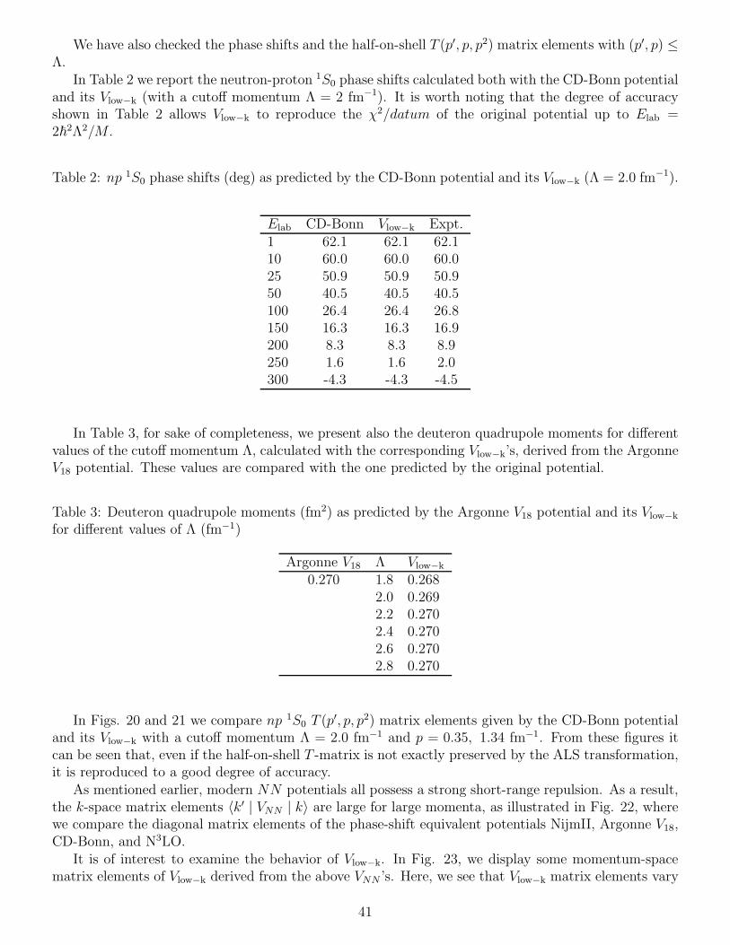
We have also checked the phase shifts and the half-on-shell T (p′, p, p2) matrix elements with (p′, p) ≤Λ.
In Table 2 we report the neutron-proton 1S0 phase shifts calculated both with the CD-Bonn potentialand its Vlow−k (with a cutoff momentum Λ = 2 fm−1). It is worth noting that the degree of accuracyshown in Table 2 allows Vlow−k to reproduce the χ2/datum of the original potential up to Elab =2~2Λ2/M .
Table 2: np 1S0 phase shifts (deg) as predicted by the CD-Bonn potential and its Vlow−k (Λ = 2.0 fm−1).
Elab CD-Bonn Vlow−k Expt.1 62.1 62.1 62.110 60.0 60.0 60.025 50.9 50.9 50.950 40.5 40.5 40.5100 26.4 26.4 26.8150 16.3 16.3 16.9200 8.3 8.3 8.9250 1.6 1.6 2.0300 -4.3 -4.3 -4.5
In Table 3, for sake of completeness, we present also the deuteron quadrupole moments for differentvalues of the cutoff momentum Λ, calculated with the corresponding Vlow−k’s, derived from the ArgonneV18 potential. These values are compared with the one predicted by the original potential.
Table 3: Deuteron quadrupole moments (fm2) as predicted by the Argonne V18 potential and its Vlow−k
for different values of Λ (fm−1)
Argonne V18 Λ Vlow−k
0.270 1.8 0.2682.0 0.2692.2 0.2702.4 0.2702.6 0.2702.8 0.270
In Figs. 20 and 21 we compare np 1S0 T (p′, p, p2) matrix elements given by the CD-Bonn potential
and its Vlow−k with a cutoff momentum Λ = 2.0 fm−1 and p = 0.35, 1.34 fm−1. From these figures itcan be seen that, even if the half-on-shell T -matrix is not exactly preserved by the ALS transformation,it is reproduced to a good degree of accuracy.
As mentioned earlier, modern NN potentials all possess a strong short-range repulsion. As a result,the k-space matrix elements 〈k′ | VNN | k〉 are large for large momenta, as illustrated in Fig. 22, wherewe compare the diagonal matrix elements of the phase-shift equivalent potentials NijmII, Argonne V18,CD-Bonn, and N3LO.
It is of interest to examine the behavior of Vlow−k. In Fig. 23, we display some momentum-spacematrix elements of Vlow−k derived from the above VNN ’s. Here, we see that Vlow−k matrix elements vary
41

0.0 0.5 1.0 1.5 2.0
p’ [fm–1
]
–120
–90
–60
–30
T(p
’,p,p
2 ) [M
eV fm
3 ]
1S0
Elab = 10 MeV
Fig. 20: (Color online) Comparison of the half-on-shell T (p′, p, p2) matrix elements (continuous line)with those of Tlow−k(p
′, p, p2) for p = 0.35 fm−1 (Elab = 10 MeV). The asterisk indicates the on-shellmatrix element. The cutoff momentum is Λ = 2 fm−1.
0.0 0.5 1.0 1.5 2.0
p [fm–1
]
–12
–8
–4
0
T(p
’,p,p
2 ) [M
eV fm
3 ]
1S0
Elab = 150 MeV
Fig. 21: (Color online) As in Fig. 20, but for p = 1.34 fm−1 (Elab = 150 MeV).
42
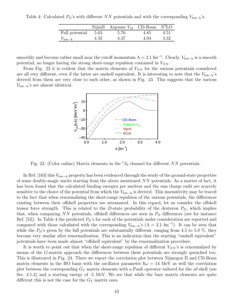
Table 4: Calculated PD’s with different NN potentials and with the corresponding Vlow−k’s.
NijmII Argonne V18 CD-Bonn N3LOFull potential 5.63 5.76 4.85 4.51Vlow−k 4.32 4.37 4.04 4.32
smoothly and become rather small near the cutoff momentum Λ = 2.1 fm−1. Clearly, Vlow−k is a smoothpotential, no longer having the strong short-range repulsion contained in VNN .
From Fig. 22 it is evident that the matrix elements of VNN for the various potentials consideredare all very different, even if the latter are onshell equivalent. It is interesting to note that the Vlow−k’sderived from them are very close to each other, as shown in Fig. 23. This suggests that the variousVlow−k’s are almost identical.
0.0 1.0 2.0 3.0 4.0
k [fm–1
]
–45
–30
–15
0
15
VN
N(k
,k)
[MeV
fm3 ]
CD–Bonn Argonne V18
NijmII N
3LO
Fig. 22: (Color online) Matrix elements in the 1S0 channel for different NN potentials.
In Ref. [163] this Vlow−k property has been evidenced through the study of the ground-state propertiesof some doubly-magic nuclei starting from the above mentioned NN potentials. As a matter of fact, ithas been found that the calculated binding energies per nucleon and the rms charge radii are scarcelysensitive to the choice of the potential from which the Vlow−k is derived. This insensitivity may be tracedto the fact that when renormalizing the short-range repulsion of the various potentials, the differencesexisting between their offshell properties are attenuated. In this regard, let us consider the offshelltensor force strength. This is related to the D-state probability of the deuteron PD, which impliesthat, when comparing NN potentials, offshell differences are seen in PD differences (see for instanceRef. [53]). In Table 4 the predicted PD’s for each of the potentials under consideration are reported andcompared with those calculated with the corresponding Vlow−k’s (Λ = 2.1 fm−1). It can be seen thatwhile the PD’s given by the full potentials are substantially different, ranging from 4.5 to 5.8 %, theybecome very similar after renormalization. This is an indication that the starting “onshell equivalent”potentials have been made almost “offshell equivalent” by the renormalization procedure.
It is worth to point out that when the short-range repulsion of different VNN ’s is renormalized bymeans of the G-matrix approach the differences between these potentials are strongly quenched too.This is illustrated in Fig. 24. There we report the correlation plot between Nijmegen II and CD-Bonnmatrix elements in the HO basis with the oscillator parameter ~ω = 14 MeV as well the correlationplot between the corresponding GT matrix elements with a Pauli operator tailored for the sd shell (seeSec. 4.1.2) and a starting energy of -5 MeV. We see that while the bare matrix elements are quitedifferent this is not the case for the GT matrix ones.
43

0.0 0.5 1.0 1.5 2.0
p [fm–1
]
–60
–45
–30
–15
0
15
Vlo
w–k
(p,p
) [M
eV fm
3 ]
– CD–Bonn – Argonne V18 – Nijmegen II – N
3LO
Fig. 23: (Color online) As in Fig. 22, but for the respective Vlow−k’s with a cutoff momentum Λ = 2.1fm−1.
–10.0 –8.0 –6.0 –4.0 –2.0 0.0 2.0 4.0 6.0 8.0 10.0
Nijmegen II [MeV]
–10.0
–8.0
–6.0
–4.0
–2.0
0.0
2.0
4.0
6.0
8.0
10.0
CD
–Bon
n [M
eV]
bare VNN
GT matrix
Fig. 24: (Color online) Correlation plots between Nijmegen II and CD-Bonn matrix elements andbetween the corresponding GT matrix elements (see text for details). The red and blue dots correspondto bare VNN and GT -matrix elements, respectively.
44

Before closing this section, a brief discussion of Vlow−k in the framework of the RG-EFT approachmay be in order. A main point of the RG-EFT approach is that low-energy physics is not sensitiveto fields beyond a cutoff scale Λ. Thus for treating low-energy physics, one just integrates out thefields beyond Λ, thereby obtaining a low-energy effective field theory. In RG-EFT, this integrationout, or decimation, generates an infinite series of counter terms [158] which is a simple power series inmomentum
The question as to wether the decimation of high-momentum modes in the derivation of Vlow−k
generates a series of counter terms has been recently investigated in Refs. [164] and [165]. In thesestudies it is assumed that Vlow−k can be expressed as
Vlow−k(q, q′) ≃ VNN (q, q
′) + Vcounter(q, q′); (q, q′) ≤ Λ , (139)
where the counter potential is given as a power series
Vcounter(q, q′) = C0+C2q
2+C ′2q
′2+C4(q4+ q′4) +C ′
4q2q′2+C6(q
6+ q′6) +C ′6q
4q′2+C ′′6 q
2q′4+ ... (140)
The counter term coefficients are determined using standard fitting techniques so that the righthand side of Eq. (139) provides a best fit to the left-hand side of the same equation. In Ref. [164] thisfitting was performed over all partial wave channels and a consistently good agreement was obtained.
An examination of the counter terms was made in [164, 165], where the coefficients of some of themare also listed. A main result is that the counter terms are all rather small except for C0 and C2 of theS waves. This is consistent with the RG-EFT approach where the counter term potential is given as adelta function plus its derivatives [158].
5 Realistic shell-model calculations
5.1 The early period
As discussed in the Introduction, while the first attempts to derive the shell-model effective interactionfrom the free NN potential go back to some forty years ago, the practical value of this approach hasemerged only during the last decade or so. On this basis, we may call the “early period” that extendingover the previous three decades. It is the aim of this section to give a brief survey of the main effortsand developments made in the field during this long period of time.
The first attempt to perform a realistic shell-model calculation may be considered the one by Dawson,Talmi and Walecka [17]. They chose 18O as testing ground and approximately solved a Bethe-Goldstoneequation for the wave function of the two valence neutrons using the free NN potential of Brueckner-Gammel-Thaler [142] which contains a hard core. This initial approach, in which the effective interactionwas simply taken to be the Brueckner reaction matrix, was followed by several authors [166, 167, 168,169]. In this context, the merit of the various methods used to obtain the nuclear reaction matrixelements was a matter of discussion [170, 171, 172, 173].
A quantitative estimate of the core polarization effects was first given by Bertsch [174], who found,for the Kallio-Kolltveit force [168], that they can produce a correction to the interaction of two valencenucleons in 18O and 42Sc as large as 30% of the G-matrix interaction. Soon afterwards a turning pointin the development of the field was marked by the work of Kuo and Brown [18], who derived an sd-shell effective interaction from the Hamada-Johnston potential [63]. After having carefully evaluatedthe reaction matrix elements for this potential, they took into account the corrections arising fromthe one-particle-one-hole (1p − 1h) excitation of the 16O core (the so-called “bubble diagram” G1p1h).Comparison of the calculated and experimental spectra of 18O and 19F provided clear evidence of thecrucial role played by the core polarization.
45
This remarkable achievement prompted the derivation of effective interactions for nuclei in othermass regions, such as the calcium [175], nickel [176, 177] and lead region [178, 179, 180]. These effectiveinteractions were all deduced from the Hamada-Johnston potential by use of the G-matrix theoryand including core-polarization effects. In this context, the individual effects of the various second-order diagrams were studied [181, 175] and the conclusion was reached that the inclusion of the corepolarization diagram, G1p1h, is generally sufficient to obtain a satisfactory agreement between calculatedand experimental spectra [182].
The substantial soundness of the effective interactions derived along the lines of the Kuo-Brownapproach is evidenced by the fact that, with empirical modifications, they have been used in a numberof successful shell-model calculations to date. This has brought about various “semi-realistic” versionsof the original Kuo-Brown interaction. In this connection, it is worth pointing out that these empiricalmodifications concern essentially the monopole parts of the effective interaction, as described in detailin Ref. [183], where the KB1, KB2, and KB3 interactions were introduced and applied to the study offp-shell nuclei. This kind of approach, which is still favored by several authors, especially in the contextof large scale shell model calculations, is outside the scope of the present article. We only mention herethat recently three-body monopole corrections to realistic forces have been considered as a simple wayto avoid a full treatment of three-body forces [184]. For a detailed discussion of the various effectiveinteractions and the results of several applications, the reader is referred to the review papers by Brown[46], Otsuka et al. [48], Talmi [5], and Caurier et al. [47], where a full list of references can also befound.
It is interesting to note that in spite of the very encouraging results produced by the first generationof realistic shell-model calculations, the general attitude of the workers in the field was rather pessimistic.This is well reflected in the final statements made by Kirson in his Summary talk [185] at the 1975Tucson International Conference:
“To summarize my summary, I would say that there are definitely major obstacles in theway of doing really convincing calculations. We have a theory, we are aware of the weaknessof our computations, and we should certainly invest the effort needed to plug the moreobvious holes. But we should recognize the lack of precision inherent in our inability togo to high orders in perturbation theory and adopt more qualitative methods of extractinginformation and gaining understanding. New ideas, new viewpoints are much needed. Weshould also try to withstand the temptations of seductive 18O, and pay some attention toother systems.”
The aim of the Tucson Conference [186] was to define the current status of effective interaction andoperator theory in the mid 1975s. The main issues of this Conference were expounded in the subsequentexcellent review by Ellis and Osnes [126]. As it emerges from the first three talks [187, 188, 189] presentedat the Tucson Conference and as mentioned in Sec. 3, in the years around 1970 the theoretical basesfor an energy-independent derivation of the effective interaction were laid down within the frameworkof the time-independent [117] as well as time-dependent [120, 121] perturbation theory. At the sametime, the problems inherent in the practical application of the theory became a matter of discussion.In this context, considerable effort was made to study the convergence properties of the perturbativeapproach to the derivation of the effective interaction. As representative examples for these studies,we may mention here the works of Refs. [190, 191, 192, 193]. In the first of these works all significantterms through third order and a few selected fourth-order terms in the G matrix were calculated andthe convergence order-by-order of the perturbation series was investigated, while in the second one thefocus was on the convergence rate of the sum over intermediate-particle states in the second-order corepolarization contribution to the effective shell-model interaction. In the third work the authors raisedthe problem of the divergence of the perturbation series due to the occurrence of the so-called “intruderstates”.
46

A most important turn in the field of realistic shell-model calculations resulted from the explicitinclusion [194, 123] of the folded diagrams in the derivation of the effective interaction within theframework of the Kuo, Lee, and Ratcliff theory [121]. In these works, starting from a realistic G matrix,effective interactions for sd-shell nuclei were derived by means of the folded-diagram expansion, andemployed in calculations for A = 18 to 24. Note that in Ref. [123] the very convenient method proposedin [130] (see Sec. 3.3) was used to sum up the folded diagram series. It turned out that the contributionof the folded diagrams to the effective interaction is quite large, typically about 30%. In the earlierstudy [194] the G matrix was obtained starting from the Reid soft core potential while in the laterstudy [123] both this potential and the Paris potential were used. It may be worth noting that thislatter paper was the first one where the Paris potential was employed in a microscopic calculation offinite open-shell nuclei.
As pointed out in Sec. 2.1, the advent of advanced meson-theoretic NN potentials, such as the Parisand Bonn ones, was instrumental in reviving the interest in the realistic effective interactions duringthe 1980s. In this context, a main issue was the sensitivity of nuclear structure calculations to thestrength of the tensor-force component contained in the NN potential, for which a practical measureis the predicted D-state probability of the deuteron PD (see Sec. 2.1).
Earlier work on this problem was done by Sommermann et al [195] who reexamined the intermediatestate convergence problem for the core polarization diagram in the expansion of an effective shell-modelinteraction using the Bonn-Julich (MDFP∆2) potential [196, 197] in comparison to the Reid soft-coreinteraction [64]. It is a remarkable achievement of this work to have shown that the so-called Vary-Sauer-Wong effect, namely the slow rate of convergence found for the Reid potential [191, 198], was ofnegligible importance for the Bonn-Julich potential, as a consequence of the much weaker tensor forcecontained in the latter.
Some ten years later, using a G-matrix folded-diagram method, the sd-shell effective interaction wasderived from various potentials and applied to calculate the spectra of some light sd-shell nuclei [199].In particular, the three variants of the OBE parametrization of the Bonn full model, Bonn A, Bonn B,and Bonn C, differing in the strength of the tensor force (see Sec. 2.1) as well as the Paris potential,were considered. It turned out that the best agreement with experiment was achieved with the weakesttensor force potential (Bonn A).
The development of more realistic NN potentials, such as the Bonn and Paris potentials, led also inthe early 1990s to new studies of the role of the third- and higher-order perturbative contributions tothe effective interaction, which had been investigated some twenty years before in the work of Ref. [190].Within the framework of the folded diagram theory, the inclusion of the third-order diagrams in G inthe calculation of the Q-box was studied and the order-by-order convergence of the effective interactionin terms of the mass number A was examined [200, 201, 202, 203]. The main findings of the last study ofthis series [203] were that the convergence of the perturbation expansion seems to be rather insensitiveto the mass number and that the effects of third-order contributions in the T = 1 channel are almostnegligible. We refer to Ref. [45] for a review of the status of the theory of realistic effective interactionsin the mid 1990s.
We have given above a brief review of the great deal of work done in the field of realistic shell-modelcalculations during what we have called, somewhat arbitrarily, the “early period”. Before finishing thissubsection, a word is in order concerning this choice of presentation, which, in our opinion, reflectshow hard it has been to make this kind of calculations a reliable tool for quantitative nuclear structurestudies.
We draw the reader’s attention to the fact that, after the calculations performed by Kuo andcollaborators from the mid 1960’s up to the mid 1970’s [175, 176, 177, 178, 179, 180], practically noother calculations were done for about two decades having as only aim a detailed description of nuclearstructure properties. This lack of confidence in the predictive power of realistic effective interactions iswell evidenced by the fact that in almost all the papers on this subject published from the mid 1970’s up
47

to about the early 1990’s, the focus has been on nuclei of the sd-shell, considered as a necessary testingground for the effective interaction before embarking on a more ambitious program of applications. Inthis connection, the warning by Kirson (see above citation) against the temptations of seductive 18Oacquires a particular significance.
5.2 Modern calculations
As discussed in the previous subsection, during the 1980s a substantial progress was made in thepractical application of shell model with realistic effective interactions. This has resulted in a newgeneration of realistic shell-model calculations oriented to the study of the spectroscopic properties ofnuclei in various mass regions.
The first attempts in this direction focused on the Sn isotopes [204, 45, 205], in particular on theneutron deficient ones. In the work of Ref. [204] the Bonn A potential was used while in that of Ref. [45]results obtained with the stronger tensor-force versions of this potential (Bonn B and Bonn C) werealso reported. In both these works all two-body diagrams through third order in the G matrix wereincluded in the Q-box. In the study of Andreozzi et al. [205] both the Paris and Bonn A potentialswere employed and the Q-box was taken to be composed of diagrams through second order in G (acomparative discussion of the above studies can be found in [205]). The results of these initial “modern”calculations, in particular those obtained with the Bonn A potential, turned out to be in remarkablygood agreement with the experimental data.
These achievements encouraged further work along these lines. In the few following years realisticshell-model calculations were carried out for a number of nuclei around doubly magic 100Sn [134], 132Sn[206, 207, 208, 209], and 208Pb [210, 211, 212]. Note that in all these calculations, except the one ofRef. [209] where the CD-Bonn 1996 potential [87] was employed, the effective interaction was derivedfrom the Bonn A potential. We refer to Covello et al. [39] for a survey of the status of realistic shell-model calculations at the end of the 1990s. Suffice it to say here that the rms deviation for the spectraof 15 medium- and heavy-mass nuclei reported in this paper is in 7 cases less than 100 keV, only in onecase reaching 165 keV.
The success achieved by these calculations gave a clear-cut answer to the crucial, long-standingproblem of how accurate a description of nuclear structure properties can be provided by realisticeffective interactions, opening finally the way to a more fundamental approach to the nuclear shellmodel than the traditional, empirical one.
As is well known, much attention is currently being focused on nuclei in the regions of shell closuresoff stability, as they allow to explore for possible shell-structure modifications when approaching theproton and neutron drip lines. The experimental study of these nuclei is very difficult, but in recentyears new data have become available for some of them, which provide a challenging testing groundfor realistic effective interactions. Starting in the early 2000s, several “exotic” nuclei around doublymagic 100Sn and 132Sn have been studied employing realistic effective interactions derived from the high-precision CD-Bonn NN potential [88]. In the first paper of this series [213] shell-model calculationswere performed for Sn isotopes beyond N = 82, in particular the heaviest Sn isotope known to date,134Sn. In this work, similarly to what had been done in their previous papers, the authors employed aG-matrix folded-diagram formalism. A very good agreement was found between the calculated resultsand the available experimental data.
A most important turn in the derivation of the effective interaction from the free NN potential hasresulted from the development of the Vlow−k approach (see Sec. 4.2). This approach to renormalize theshort-range repulsion of VNN has been recently used in several calculations. Attention has been focusedon exotic nuclei neighboring 100Sn [214], and 132Sn [215, 216, 217, 163, 218, 219]. Actually, most of theseworks are concerned with nuclei in the latter region, for which there are new interesting experimentaldata. The agreement between theory and experiment has turned out to be very good in all cases. This
48

supports confidence in the predictions of these realistic calculations, which may therefore stimulate andbe helpful to, future experiments. To illustrate this important point, we shall review in Sec. 5.3.3 someselected results for 132Sn neighbors with neutrons beyond the 82 shell.
While most of the realistic shell-model calculations carried out in last few years have employedeffective interactions derived from the CD-Bonn NN potential, some attempts to put to the test chiralpotentials have also been made. Representative examples for these studies are the works of Refs. [220,221, 222, 223], all of them making use of the Vlow−k renormalization method. Actually, only in [220],where the NNLO Idaho potential [104] was used, shell model calculations for various two valence-particlenuclei were performed. In the other three works [221, 222, 223] ground-state properties of doubly magicnuclei 4He, 16O, and 40Ca were calculated within the framework of the Goldstone expansion [122] withthe N3LO potential [102]. The results obtained in [220] turned out to be comparable to those producedby effective interactions derived from the CD-Bonn potential. Clearly, this is related to the importantquestion of how much nuclear structure results depend on the NN potential one starts with. We shalldiscuss this point in Sec. 5.3.2.
5.3 Results
5.3.1 Comparison between G-matrix and Vlow−k approaches
As evidenced by the discussion given in Secs. 5.1 and 5.2, for about forty years the Brueckner G matrixrepresented practically the only tool to renormalize the repulsive core contained in the NN potential.After its introduction, the Vlow−k potential has been readily seen as an alternative to the G matrix. Infact, Vlow−k is a smooth free-space potential and its matrix elements between unperturbed two-particlestates can be directly used as input to the Q-box folded-diagram procedure of Sec. 3. Therefore, a mainissue has been to assess the merit of the Vlow−k approach in practical applications.
First work along this line was done by Kuo et al. [224], who carried out shell-model calculationsfor 18O using two-body matrix elements of effective interactions derived from the Bonn A and Parispotentials. Other studies [225, 43, 226] were then performed which, starting from the CD-Bonn poten-tial, extended the comparison between the G matrix and Vlow−k approaches to nuclei heavier than 18O.In particular, the calculations of Ref. [225] concern 132Sn neighbors, while results for 18O, 134Te, and135I are presented in [43]. A comparison between the G matrix and Vlow−k spectra for the heavy-massnucleus 210Po can be found in [226]. In all these calculations the cutoff parameter Λ is chosen in thevicinity of 2 fm−1.
It has been a remarkable finding of all these studies that the Vlow−k results are as good or even slightlybetter than the G-matrix ones. The rather close similarity between the results of the two approachesfinds an exception for the Paris potential [224]. We shall comment on this point in Sec. 5.3.2. It is alsoimportant to point out that the Vlow−k approach appears to work equally well in different mass regions.A detailed description of the above mentioned calculations can be found in the cited references. Here,for the sake of completeness, we report two examples concerning 18O and 134Te, which are both takenfrom [43], where more details about the calculations can be found.
The experimental and calculated spectra of 18O including the five lowest-lying states, and those of134Te with the eight lowest-lying states are reported in Figs. 25 and 26, respectively. The calculatedspectra have been obtained from the CD-Bonn potential through both the Vlow−k and G-matrix folded-diagram approaches. As for the Vlow−k calculations, two values of the cutoff momentum have been used,Λ = 2.0 and 2.2 fm−1. For 18O we have adopted a model space with the two valence neutrons in the(0d5/2, 0d3/2, 1s1/2) shell, while for 134Te the two valence protons are allowed to occupy the levels ofthe (0g7/2, 1d5/2, 1d3/2, 2s1/2, 0h11/2) shell. In both cases the SP energies are taken from experiment, inparticular from the spectra of 17O and 133Sb for the sd and sdgh shells, respectively. The energy ofthe 2s1/2 proton level, which is still missing, is from the study by Andreozzi et al. [206]. Note that in
49

Figs. 25 and 26 the energies are relative to the ground state of the neighboring doubly closed nucleus 16Oand 132Sn, respectively, with the mass-excess values for 17O and 133Sb needed for the absolute scaling ofthe SP energies coming from Refs. [227] and [228]. As for 134Te, the Coulomb contribution was takeninto account by adding to the CD-Bonn effective interaction the matrix element of the Coulomb forcebetween two g 7
2
protons with J = 0.
-12.0
-11.0
-10.0
-9.0
-8.0
E(M
eV
)
Expt. Λ = 2.0 Λ = 2.2 G matrix
18O
0+
2+
4+
0+
2+
0+
2+
4+
0+
2+
0+
2+
4+
0+
2+
0+
2+
4+
0+
2+
Fig. 25: Low-lying states in 18O.
As pointed out above, we see from Figs. 25 and 26 that the Vlow−k and G-matrix results are ratherclose to each other and in quite good agreement with experiment. It is worth noting that the Vlow−k
results for the two values of Λ do not differ significantly. We shall come back to this point later.In this context, we may also mention the work of Refs. [229] and [230], where harmonic-oscillator
matrix elements of the Vlow−k potential and G matrix are compared in 4 major shells. It was found thatboth the T = 0 and T = 1 matrix elements are very similar.
On the above grounds, the conclusion is reached that the Vlow−k approach is a reliable way torenormalize the bare NN potential before employing it in the derivation of the shell-model effectiveinteraction.
Another relevant point to be stressed is that the Vlow−k is far easier to be used than the G matrix.In fact, Vlow−k is a soft NN potential and as such does not depend either on the starting energy or onthe model space, as is instead the case of the G matrix, which is defined in the nuclear medium. Thishas the desirable consequence that the Vlow−k matrix element to be used in an interaction vertex of agiven Q box diagram is completely determined by the incoming and outcoming lines attached to thevertex under consideration. Hence, it does not depend on any other part of the diagram. Also, it isworth noting that the same Vlow−k can be used in different mass regions.
Finally, when considering the features of the Vlow−k approach, one has also to keep in mind that, asdiscussed in Sec. 4.2.3, different NN potentials lead to low-momentum potentials which are remarkablysimilar to each other. In the same section, we have showed that the differences between the differentpotentials are also quenched within the G matrix approach. This will be further discussed in Sec. 5.3.2.
We conclude by mentioning that the Vlow−k approach has also proved to be an advantageous alter-native to the G matrix in the calculation of the ground-state properties of doubly closed nuclei. Asis well known, the traditional approach to this problem is the Brueckner-Hartree-Fock (BHF) theory.
50

In the study of Ref. [221] it has been showed that the Vlow−k is suitable for being used directly in theGoldstone expansion. Good results for 16O and 40Ca were obtained by solving the Hartree-Fock (HF)equations for Vlow−k and then using the resulting self-consistent basis to compute higher-order Goldstonediagrams. In this connection, it should be mentioned also the work of Ref. [231], where use was madeof the Vlow−k potential in a HF and BHF approach to evaluate the binding energy and the saturationdensity of nuclear matter and finite nuclei. Their conclusion was that for nuclear matter at small andmedium densities as well as for finite nuclei HF and BHF results with Vlow−k are nearly identical.
-20.5
-19.5
-18.5
E(M
eV
)
Expt. Λ = 2.0 Λ = 2.2 G matrix
134Te
0+
2+
4+
6+
6+
2+
4+
1+
0+
2+
4+
6+
6+
1+
2+
4+
0+
2+
4+
6+
6+
1+
4+
2+
0+
2+
4+
6+
6+
1+
2+
4+
Fig. 26: Low-lying states in 134Te.
5.3.2 Calculations with different NN potentials
As discussed in Sec. 5, a main problem relevant to realistic shell-model calculations has been to assessthe accuracy of the effective interaction derived from the NN potential. However, it is also an importantissue what information comes out on the NN potential from this kind of calculations. As we have seenin Sec. 2, from the early 1950s on several different potentials have been constructed. The potentialsof the last generation all fit equally well the NN phase shifts, but, except for the OPE tail, theyare quite different from each other. Actually, these potentials are well-constrained by the deuteronproperties and the NN scattering data for Elab < 350 MeV and therefore their offshell behavior issubject to ambiguities. This is reflected in the different values predicted for the D-state probability ofthe deuteron PD (see Sec. 2) as well as in the different binding energies calculated for A = 3, 4 systems[232]. In fact, for A > 2 the interaction may be off the energy shell since two nucleons may have differentenergies before and after they interact.
In this context, it is of great interest to perform nuclear structure calculations to see to which extentthe differences between NN potentials persist once the short-range repulsion is renormalized throughthe G-matrix or the Vlow−k approach. This problem has long been investigated by studying propertiesof both nuclear matter and doubly closed nuclei. A list of references on this subject can be found inthe work of Ref. [222], which we have briefly discussed in Secs. 4.2.3 and 5.2. As for open-shell nuclei,some attempts have been made within the framework of the shell model.
51

In the early work by Sommermann et al. [195], the comparison between Bonn-Julich and Reid resultsaimed at investigating the intermediate-state convergence problem, as discussed in Sec. 5.1. The paperby Shurpin et al. [123] had instead as a main purpose to compare the spectra of several sd-shell nucleicalculated with two different potentials, Paris and Reid. The results showed that the Paris potentialwas as good as, if not better than, the Reid potential. The idea of comparing shell-model calculationswith different NN potentials was revived at the end of the 1980s. In the works of Refs. [233, 199] and[234] sd-shell nuclei were studied using as input several different NN potentials, all constructed beforethe 1990s. These works were based on the use of the reaction matrix G to derive the effective interactionthrough the Q-box folded-diagram method, including up to second-order diagrams. The outcome ofthese studies was that the effective interaction matrix elements become more attractive when a NNpotential with a weaker tensor-force strength is used. Jiang et al. [199] noted that the nonlocality ofthe potential gives a further contribution in this direction. All these calculations indicated in generalthat the best agreement with experiment was produced by the Bonn potential.
A confirmation of the important role played by weaker tensor force potentials came out from thepaper of Ref. [205], where Paris and Bonn A results for neutron deficient Sn isotopes are compared. Abetter agreement with experiment was obtained with the Bonn A potential. The merit of potentialswith weak tensor force was also evidenced in [45], who performed realistic shell-model calculations fornuclei in the mass regions of 16O, 40Ca, and 100Sn using the three variants (A, B, and C) of the Bonnpotential.
A comparative study of shell-model results obtained from different NN potentials, including thehigh-precision CD-Bonn potential, was made for the first time in [235]. In this paper, the nucleus 134Tewas used as a testing ground to investigate the effects of the CD-Bonn potential with respect to thoseof the three potentials Bonn A, Paris, and Nijm93. As in all previous calculations, it was found that aweak tensor force leads to a better description of nuclear structure properties. Furthermore, it turnedout that the calculated spectra, except that obtained from the Paris potential, are only slightly differentfrom each other.
All the above calculations made use of the reaction matrix G and their results provide evidencethat the differences existing between various potentials are quenched by the G-matrix renormalizationprocedure (see Fig. 24). One may wonder what happens when the Vlow−k potential is used. The firstanswer to this question may be found in [224], where the Vlow−k approach is used to calculate the Parisand Bonn A spectra for 18O. It is interesting to note that these two spectra are much closer to eachother than those obtained with the G matrix approach [199]. This reflects the fact that the Vlow−k
procedure is more effective in reducing the differences between the two potentials than the G-matrixapproach. The matrix elements in the 3S1 channel for both Paris and Bonn A potentials are reportedin Fig. 1 of [224], where it is shown that they become similar after the Vlow−k renormalization, the latterbeing much larger for the strongly repulsive Paris potential.
In Sec. 4.2.3 (see Figs. 22 and 23), we have reported a similar comparison in the 1S0 channel forthe chiral potential N3LO and the three high-precision potentials CD-Bonn, NijmII, and Argonne V18.The differences between the matrix elements of these potentials practically disappear when the Vlow−k
matrix elements are considered. On these grounds one expects that shell-model effective interactionsderived from phase-shift equivalent NN potentials through the Vlow−k approach should lead to verysimilar results.
This we have verified by calculating the spectra of 134Te starting from the CD-Bonn, NijmII, andArgonne V18 potentials. For all the three Vlow−k’s derived from these NN potentials, use has beenmade of the same cutoff momentum Λ = 2.2 fm−1. Other details on how these calculations have beenperformed may be found in Sec. 5.3.3, where we present results for nuclei beyond 132Sn, which havebeen obtained using the CD-Bonn potential.
In Fig. 27, the three calculated spectra are shown and compared with the experimental one. Notethat, with respect to Fig. 26, the energies are relative to the ground state and higher lying levels are
52

0
1
2
3
4
E(M
eV)
Expt. CD-Bonn NijmII Argonne V18
134Te
0+
2+
4+
6+
6+2+
4+
1+
3+
5+
2+
9−
7−5−5+6−8−
0+
2+
4+
6+
6+
4+
,2+
1+
,3+
5+
2+
9−
5+7−5−6−
8−
0+
2+
4+
6+
6+
4+,2+
1+,3+
5+
2+
9−
5+7−5−6−8−
0+
2+
4+
6+
6+
4+
,2+
1+
,5+
3+
2+
9−
5+7−5−6−
8−
Fig. 27: Spectrum of 134Te. Predictions by various NN potentials are compared with experiment.
53

0
1
2
3
E
(
M
e
V
)
Expt. Cal .
134
Sn
0
+
2
+
4
+
6
+
8
+
0
+
2
+
4
+
6
+
8
+
Fig. 28: Experimental and calculated spectra of 134Sn.
included. We see that the calculated spectra are very similar, the differences between the predictedenergies not exceeding 80 keV. It is also seen that the agreement with experiment is very good for allthe three potentials. In fact, the rms deviation is 115, 128, and 143 keV for CD-Bonn, Argonne V18,and NijmII, respectively.
Finally, it is of interest to make a few comments regarding the value of the cutoff momentum Λ.In Sec. 4.2.3 the plausibility of using a value in the vicinity of 2 fm−1 was discussed. It was alsoshown in Sec. 5.3.1 that shell-model results do not change significantly when varying Λ from 2 to 2.2fm−1. A preliminary study of the dependence of shell-model results on Λ can be found in the work ofRef. [236], where results for 134Te are reported using the CD-Bonn, Argonne V18, and NijmII potentialswith Λ varying over a rather large range (1.5-2.5 fm−1). It has been found that the best agreementwith experiment for each of these three potentials corresponds to a somewhat different value of Λ.However, changes around this value do not significantly modify the quality of agreement for all thethree potentials. As an example, the rms deviation for NijmII remains below 150 keV for any value ofΛ between 1.8 and 2.2 fm−1 This subject deserves certainly further studies.
5.3.3 Neutron rich nuclei beyond 132Sn: comparing theory and experiment
The study of exotic nuclei is a subject of a current experimental and theoretical interest. Experimentalinformation for nuclei in the vicinity of 78Ni, 100Sn, 132Sn, which have been long inaccessible to spec-troscopic studies, is now available thanks to new advanced facilities and techniques. The advent ofradioactive ion beams is opening new perspectives in this kind of studies. Nuclei in the regions of shellclosures are a source of direct information on shell structure. New data offer therefore the opportunityto test the shell model and look for a possible evolution of shell structure when going toward proton orneutron drip lines.
This is stimulating shell-model studies in these regions. Several realistic shell-model calculationshave been recently performed for nuclei around 100Sn and 132Sn, as mentioned in Sec. 5.2. We reporthere some selected results on 132Sn neighbors with N > 82. More precisely, we consider the three nuclei134Sn, 134Sb, and 135Sb, which have been very recently studied in [219], [218], and [163], to which werefer for a more detailed discusssion.
The experimental data which have been now become available for these neutron-rich nuclei may
54

0.0
0.5
1.0
E
(
M
e
V
)
Expt. Cal .
134
Sb
0
1
7
2
3
5
4
6
1
2
0
1
2
7
3
5
4
6
1
2
Fig. 29: Experimental and calculated spectra of 134Sb.
suggest a modification in the shell structure. They are, in fact, somewhat different from what onemight expect by extrapolating the existing results for N < 82, and as a possible explanation a changein the single-proton level scheme has been suggested. The latter, caused by a more diffuse nuclearsurface, may be seen as a precursor of major effects which should show up at larger neutron excess.
We shall see now that the properties of these three nuclei are all well accounted for by a shell-model calculation with a two-body effective interaction derived from a modern NN potential. In sodoing, we evidence the merit of realistic shell-model calculations, showing, at the same time, thatthere is no need to invoke new effects to describe few-valence-particle nuclei just above 132Sn. In thisconnection, it is worth mentioning that different shell-model calculations have been performed for theabove nuclei [237, 238, 239, 240, 241, 242]. None of these studies, however, has succeeded in accountingsimultaneously for the peculiar features of all the three nuclei.
In our calculations, we assume that 132Sn is a closed core and let the valence neutrons occupy the sixlevels 0h9/2, 1f7/2, 1f5/2, 2p3/2, 2p1/2, and 0i13/2 of the 82-126 shell, while for the proton the model spaceincludes the five levels 0g7/2, 1d5/2, 1d3/2, 2s1/2, and 0h11/2 of the 50-82 shell. The proton and neutronsingle-particle energies have been taken from the experimental spectra of 133Sb and 133Sn, respectively,the only exceptions being those of the s1/2 proton and i13/2 neutron levels which are still missing. Theenergy of the former, as mentioned in Sec. 5.3.1, is from [206], while that of the latter from [213].The two-body matrix elements of the effective interaction have been derived from the CD-Bonn NNpotential. This potential is renormalized by constructing the Vlow−k with a cutoff momentum Λ =2.2fm−1. The effective interaction has been then derived within the framework of the Q-box plus foldeddiagram method including diagrams up to second order in Vlow−k. The computation of these diagramsis performed within the harmonic-oscillator basis using intermediate states composed of all possiblehole states and particle states restricted to the five shells above the Fermi surface. This guaranteesthe stability of the results when increasing the number of intermediate particle states. The oscillatorparameter used is ~ω = 7.88 MeV and for protons the Coulomb force has been explicitly added to theVlow−k potential.
The experimental and calculated spectra of 134Sn, 134Sb, and 135Sb are compared in Figs. 28, 29,and 30, respectively. Note that both the calculated and experimental spectra of 134Sb include all levelslying below 1 MeV excitation energy, while for 135Sb all the yrast states have been reported. As for134Sn, only the levels reported in Fig. 28 have been observed, while in the calculated spectrum fivestates, predicted in between the 6+ and 8+ states, are omitted.
The two isotones with A = 134 are the most appropriate systems to study the effects of the effectiveinteraction. In fact, 134Sn is a direct source of information on the neutron-neutron channel while 134Sbon the proton-neutron one. The nucleus 135Sb represents a further interesting test, since it allows toinvestigate at once the role of the effective interaction in both channels.
From the above figures, we see that the experimental levels in all the three nuclei are very well
55

0
1
2
E
(
M
e
V
)
Expt. Cal .
135
Sb
7
2
+
5
2
+
3
2
+
11
2
+
9
2
+
15
2
+
19
2
+
23
2
+
7
2
+
5
2
+
3
2
+
11
2
+
9
2
+
15
2
+
19
2
+
23
2
+
Fig. 30: Experimental and calculated spectra of 135Sb.
reproduced by the theory, the discrepancies being of the order of few tens of keV for most of the states.Note that the very low-energy positions of both the first-excited 2+ and 1− states in 134Sn and 134Sb,respectively, are well accounted for, as is also the case for the low excitation energy of the 5/2+ state in135Sb. We refer to the above mentioned papers for more details on each of the three calculations and fora discussion of the structure of the states in 134Sb and 135Sb. As for the latter, it is shown in [163] thatit is the admixed nature of the 5/2+ state that explains its anomalously low position and the stronglyhindered M1 transition to the ground state. The role of the effective interaction as well as of the 5/2+
single-proton energy in determining this situation has been examined, with particular attention to theeffects induced by the proton-neutron interaction. The relevant role of the latter was also evidenced in134Sb [218]. For this nucleus, a direct relation can be established between the diagonal matrix elementsof the proton-neutron effective interaction and the calculated energies reported in Fig. 29, since thecorresponding wave functions are characterized by very little configuration mixing. In particular, theeight lowest-lying states can be identified with the eight members of the πg7/2νf7/2 multiplet whilethe two higher states, with Jπ = 1− and 2−, are the only members of πd5/2νf7/2 multiplet having anexperimental counterpart.
In this connection, it may be interesting to summarize here the analysis of the proton-neutron matrixelements reported in the work of Ref. [218]. Focusing on the πg7/2νf7/2 configuration, we examine thevarious terms which contribute to the effective interaction, namely the Vlow−k and all the second-ordertwo-body diagrams composing the Q box. It is worth pointing out that the effective interaction Veffis obtained by summing to the Q-box the folded-diagram series [see Eq. (58)], but the contributionof the latter provides a common attenuation for all matrix elements, thus not affecting the followingdiscussion.
The diagonal matrix elements of Vlow−k for the πg7/2νf7/2 configuration are reported in Fig. 31 as afunction of J together with the contributions arising from the 1p− 1h, 2p− 2h, and ladder excitations.In Fig. 32 we present for the same configuration the diagonal matrix elements of the effective interactionwhich we have obtained starting from this Vlow−k. Note that the behavior of Veff shown in Fig. 32 is quitesimilar to that of the πg7/2νf7/2 multiplet in 134Sb, whose members, as mentioned above, are almostpure. This behavior, however, is quite different from that of Vlow−k, especially as regards the 0− − 1−
spacing. This means that the second-order two-body contributions accounting for configurations leftout of the chosen model space are of key importance to renormalize the Vlow−k and get the correctbehavior. In particular, a crucial role is played by the core-polarization effects arising from the 1p− 1h
56
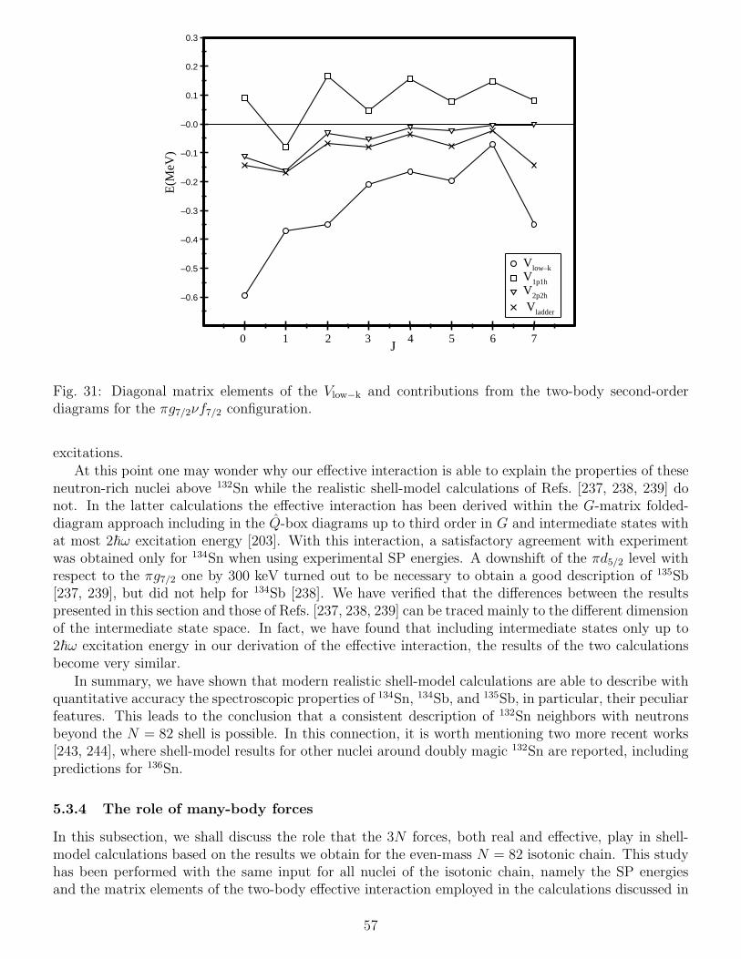
–0.6
–0.5
–0.4
–0.3
–0.2
–0.1
–0.0
0.1
0.2
0.3
E(M
eV)
J 0 1 2 3 4 5 6 7
Vlow–k V1p1h V2p2h
Vladder
Fig. 31: Diagonal matrix elements of the Vlow−k and contributions from the two-body second-orderdiagrams for the πg7/2νf7/2 configuration.
excitations.At this point one may wonder why our effective interaction is able to explain the properties of these
neutron-rich nuclei above 132Sn while the realistic shell-model calculations of Refs. [237, 238, 239] donot. In the latter calculations the effective interaction has been derived within the G-matrix folded-diagram approach including in the Q-box diagrams up to third order in G and intermediate states withat most 2~ω excitation energy [203]. With this interaction, a satisfactory agreement with experimentwas obtained only for 134Sn when using experimental SP energies. A downshift of the πd5/2 level withrespect to the πg7/2 one by 300 keV turned out to be necessary to obtain a good description of 135Sb[237, 239], but did not help for 134Sb [238]. We have verified that the differences between the resultspresented in this section and those of Refs. [237, 238, 239] can be traced mainly to the different dimensionof the intermediate state space. In fact, we have found that including intermediate states only up to2~ω excitation energy in our derivation of the effective interaction, the results of the two calculationsbecome very similar.
In summary, we have shown that modern realistic shell-model calculations are able to describe withquantitative accuracy the spectroscopic properties of 134Sn, 134Sb, and 135Sb, in particular, their peculiarfeatures. This leads to the conclusion that a consistent description of 132Sn neighbors with neutronsbeyond the N = 82 shell is possible. In this connection, it is worth mentioning two more recent works[243, 244], where shell-model results for other nuclei around doubly magic 132Sn are reported, includingpredictions for 136Sn.
5.3.4 The role of many-body forces
In this subsection, we shall discuss the role that the 3N forces, both real and effective, play in shell-model calculations based on the results we obtain for the even-mass N = 82 isotonic chain. This studyhas been performed with the same input for all nuclei of the isotonic chain, namely the SP energiesand the matrix elements of the two-body effective interaction employed in the calculations discussed in
57

–0.6
–0.4
–0.2
–0.0
E(M
eV)
J 0 1 2 3 4 5 6 7
Fig. 32: Diagonal matrix elements of the two-body effective interaction for the πg7/2νf7/2 configuration.
Sec. 5.3.3. Here, the shell-model calculations have been carried out by using the Oslo code [245].
Let us first consider the two valence-proton system 134Te. As mentioned in Sec. 2.3, a genuine 3Npotential, which may affect the one- and two-body components of the shell-model effective interactionH1
eff of Eq. (58), has never been considered explicitly. The contributions of the 3N potential to the one-body term of H1
eff may be assumed as taken into account when, as usual,the SP energies are taken fromthe experimental data. As regards the contribution of the 3N potential to the two-body component ofH1
eff , it may be reduced with an appropriate choice of the cutoff momentum Λ of the Vlow−k. In [229],it was suggested to choose Λ around 2 fm−1, since this value seems to minimize the role of the 3Npotential when calculating the 3H and 4He binding energies. In this context, it is worth recalling thathere we have used experimental SP energies and an effective interaction derived from a Vlow−k withΛ = 2.2 fm−1.
For the ground-state energy of 134Te, relative to the doubly magic 132Sn, we obtain a value of -20.796MeV to be compared with the experimental one -20.584 MeV. As regards the energy spectrum, the rmsdeviation is 0.115 MeV (see Fig. 27). These results seem to validate for many-nucleons systems thehypothesis made in [229] about the choice of Λ.
132 136 140 144 148 152 156
A
0.0
1.0
2.0
3.0
4.0
5.0
Ene
rgy
[MeV
] Expt.Theory
Fig. 33: Excitation energies of the J = 2+ yrast states for N = 82 isotones as a function of mass numberA.
58

Let us now come to nuclei with more than two valence nucleons. We know that in this case many-body terms appear in the shell-model effective interaction, even if the original potential is only atwo-body one. The effects of these terms have not yet been quantitatively evaluated [11, 38, 246, 247].However, it is generally believed that effective many-body forces have little influence on the excitationenergies, while the binding energies may be significantly affected [127]. In this connection, it may bementioned that Talmi [248] has shown that the experimental binding energies of the tin isotopes canbe reproduced quite accurately employing an empirical two- and three-body interaction.
In order to study the effective many-body forces, we have calculated the excitation energies of thelowest-lying yrast states in the even N = 82 isotones. In Figs. 33, 34, and 35, the calculated energyof the Jπ = 2+, 4+, and 6+ states, respectively, are reported as a function of the mass number A andcompared with the experimental data. It is seen that the agreement between theory and experiment isof the same quality all over the isotonic chain, thus confirming that effective many-body forces play anegligible role in the description of the relative energy spectra.
132 136 140 144 148 152
A
1.0
2.0
3.0
4.0
5.0
Ene
rgy
[MeV
] Expt.Theory
Fig. 34: Same as in Fig.33 but for J = 4+.
In Fig. 36, we report the ground-state energy per valence nucleon. It appears that the experimentaland theoretical behaviors diverge when increasing the number of protons. As in the case of tin isotopes[249], the binding energy is increasingly overestimated. This deficiency may be healed by adding a smallrepulsive monopole contribution, whose origin may be traced to effective many-body forces [248].
6 Summary and conclusions
In this paper, we have tried to give a self-contained review of the present status of shell-model calcula-tions employing two-body effective interactions derived from the free nucleon-nucleon potential. A mainfeature of this kind of calculations, which are commonly referred to as realistic shell-model calculations,is that no adjustable parameter appears in the determination of the effective interaction. This removesthe uncertainty inherent in the traditional use of empirical interactions.
As discussed in the Introduction, only in the last few years has this approach, which started inthe 1960s, acquired a reputation for being able to provide an accurate description of nuclear structureproperties. This means that to place in its proper perspective the current status of the field it is helpfulto look back and survey the difficulties faced and the progress achieved over about four decades. Thepresent review, while aimed at giving an insight into modern realistic shell-model calculations, is also
59

132 136 140 144 148 152
A
1.0
2.0
3.0
4.0
5.0
6.0
Ene
rgy
[MeV
] Expt.Theory
Fig. 35: Same as in Fig.33 but for J = 6+.
0 4 8 12 16 20 24
Zval
–11
–10
–9
–8
–7
–6
–5
–4
–3
Ene
rgy/
Zva
l [M
eV] Expt.
Theory
Fig. 36: Ground-state energies per valence proton of N = 82 isotones as a function of the valence-protonnumber Z.
60

concerned with the above aspects in regard to both the NN potential and the many-body methods forderiving the effective interaction.
As regards the first issue, in Sec. 2 we have discussed in some detail the main advances in theunderstanding of the NN interaction from the early stages of development until the current effortsbased on chiral effective field theory. This we have done to show how the advances in this field havebeen intimately related to the development of realistic nuclear structure calculations. The present stageof development is certainly enough to provide a sound starting point for a quantitative description ofnuclear structure properties. It remains a main task for the near future to assess the role of the three-body forces in many-nucleon systems. A brief discussion on this matter is given in Sec. 5.3.4 based onthe results for the even N = 82 isotones.
In Sec. 3 we have described how the shell-model effective interaction can be derived within theframework of degenerate time-dependent perturbation theory.
The problem of the short-range repulsion contained in the NN potential has been discussed inSec. 4, where, after an outline of the traditional Brueckner G-matrix method, we have described a newapproach to the renormalization of VNN , which consists in constructing a low-momentum NN potential,Vlow−k, that preserves the physics of VNN up to a cutoff momentum Λ. Since Vlow−k is already a smoothpotential, it can be used directly as input for the derivation of the shell-model effective interactioninstead of the usual G matrix. While its merit in this respect has been assessed by several calculations(Sec. 5.3.1) the NN potential Vlow−k is currently attracting much attention. On the one hand, it is beingapplied in various contexts, for instance in the study of few-body problems [250, 114]. On the otherhand, its properties are being studied in detail, in particular as regards the dependence on the originalpotential model [251, 222, 236]. Concerning shell-model calculations, results obtained with differentNN potentials using the Vlow−k approach have been presented in Sec. 5.3.2.
A main motivation for this review has been the practical success achieved by realistic shell-modelcalculations in the last few years, after a long period of hope and dismay. In Sec. 5. we have firstsurveyed the main efforts in this field going from the early to present days. We have then presented, byway of illustration, some selected results of recent calculations for nuclei around doubly magic 132Sn.These neutron-rich nuclei, which lie well away from the valley of stability, offer the opportunity for astringent test of the matrix elements of the effective interaction. The very good agreement with theavailable experimental data shown in Sec. 5.3.3 supports confidence in the predictive power of realisticshell-model calculations in the regions of shell closures off stability, which are of great current interest.
As already pointed out above, in this review our focus has been on shell-model calculations employinggenuine freeNN potentials. As a consequence of this choice, even a brief summary of the many successfulshell-model calculations employing modified versions of free NN potentials would have been beyondthe scope of the present article. Here, we have also not touched upon another important aspect of shell-model work, namely the development of new methods, such as the Monte Carlo shell model (MCSM),as well as of high-quality codes, such as ANTOINE [252], which has greatly extended the feasibilityof large-scale calculations. However, both these issues are discussed in detail in the recent article byCaurier et al. [47] while for a specialized review of the MCSM we refer to Ref. [48].
To conclude, we may say that the stage for realistic shell-model calculations is by now well set,which is a major step towards the understanding of the properties of complex nuclei in terms of theforces among nucleons. In this context, the Vlow−k approach provides a new effective tool to handle theshort-range repulsion of the free NN potential.
Acknowledgments
Helpful discussions with Gerry Brown, Scott Bogner, Jason Holt and Achim Schwenk are gratefullyacknowledged. This work was supported in part by the Italian Ministero dell’Istruzione, dell’Universita
61

e della Ricerca (MIUR), and by the U.S. DOE Grant No. DE-FG02-88ER40388.
References
[1] M.G. Mayer, Phys. Rev. 75 (1949) 1969.
[2] O. Haxel, J.H.D. Jensen and H.E. Suess, Phys. Rev. 75 (1949) 1766.
[3] M.G. Mayer and J.H.D. Jensen, Elementary theory of nuclear shell structure (John Wiley, NewYork, 1955).
[4] M.G. Mayer, Phys. Rev. 78 (1950) 22.
[5] I. Talmi, Adv. Nucl. Phys. 27 (2003) 1.
[6] S.C. Pieper et al., Phys. Rev. C 64 (2001) 014001.
[7] S.C. Pieper and R.B. Wiringa, Annu. Rev. Nucl. Part. Sci. 51 (2001) 53.
[8] P. Navratil and B.R. Barrett, Phys. Rev. C 54 (1996) 2986.
[9] P. Navratil, J.P. Vary and B.R. Barrett, Phys. Rev. Lett. 84 (2000) 5728.
[10] K. Suzuki et al., Nucl. Phys. A 567 (1994) 576.
[11] D.J. Dean et al., Prog. Part. Nucl. Phys. 53 (2004) 419.
[12] K. Kowalski et al., Phys. Rev. Lett. 92 (2004) 132501.
[13] M. Wloch et al., Phys. Rev. Lett 94 (2005) 212501.
[14] J.R. Gour et al., Phys. Rev. C 74 (2006) 024310.
[15] A. Nogga et al., Phys. Rev. C 73 (2006) 064002.
[16] P. Navratil et al., Phys. Rev. Lett. 99 (2007) 042501.
[17] J.F. Dawson, I. Talmi and J.D. Walecka, Ann. Phys. (NY) 18 (1962) 339.
[18] T.T.S. Kuo and G.E. Brown, Nucl. Phys. 85 (1966) 40.
[19] J.P. Elliott, Cargese Lectures in Physics, Vol. 3, edited by M. Jean, p. 337, Gordon and Breach,New York, 1969.
[20] I. Talmi, Rev. Mod. Phys. 34 (1963) 704.
[21] S. Cohen and D. Kurath, Nucl. Phys. 73 (1965) 1.
[22] B.H. Wildenthal, Proceedings of the International School of Physics “Enrico Fermi”, CourseXLIX, Varenna, 1976, edited by A. Bohr and R.A. Broglia, p. 383, Nort-Holland, 1977.
[23] B.H. Wildenthal, Prog. Part. Nucl. Phys. 11 (1984) 5.
[24] B.A. Brown and B.H. Wildenthal, Ann. Rev. Nucl. Part. Sci. 38 (1988) 29.
[25] B.A. Brown and W.A. Richter, Phys. Rev. C 74 (2006) 0343150.
62

[26] S.T. Belayev, Mat. Fys. Medd. Dan. Vid. Selsk. 31 (1959).
[27] L.S. Kisslinger and R.A. Sorensen, Mat. Fys. Medd. Dan. Vid. Selsk. 32 (1960).
[28] A.K. Kerman, R.D. Lawson and M.H. MacFarlane, Phys. Rev. 124 (1961) 162.
[29] L.S. Kisslinger and R.A. Sorensen, Rev. Mod. Phys. 35 (1963) 853.
[30] L.M. Green and S.A. Moszkowski, Phys. Rev. B 139 (1965) 790.
[31] R. Arvieu and S.A. Moszkowski, Phys. Rev. 145 (1966) 830.
[32] A. Plastino, R. Arvieu and S.A. Moszkowski, Phys. Rev. 145 (1966) 837.
[33] A.B. Migdal, Theory of Fermi Systems and Applications to Atomic Nuclei (Interscience, NewYork, 1967).
[34] F. Andreozzi et al., Phys. Rev. C 41 (1990) 250.
[35] F. Andreozzi et al., Phys. Rev. C 45 (1992) 2008.
[36] S.F. Tsai and T.T.S. Kuo, Phys Lett. B 39 (1972) 427.
[37] E.M. Krenciglowa and T.T.S. Kuo, Nucl. Phys. A 235 (1974) 171.
[38] T.T.S. Kuo and E. Osnes, Lecture Notes in Physics, vol. 364 (Springer-Verlag, Berlin, 1990).
[39] A. Covello et al., Acta Phys. Pol. B 32 (2001) 871.
[40] J.P. Elliott et al., Nucl. Phys. A 121 (1968) 241.
[41] A.D. Jackson and J.P. Elliott, Nucl. Phys. A 125 (1969) 276.
[42] S. Bogner, T.T.S. Kuo and L. Coraggio, Nucl. Phys. A 684 (2001) 432c.
[43] S. Bogner et al., Phys. Rev. C 65 (2002) 051301(R).
[44] S. Bogner, T.T.S. Kuo and A. Schwenk, Phys. Rep. 386 (2003) 1.
[45] M. Hjorth-Jensen, T.T.S. Kuo and E. Osnes, Phys. Rep. 261 (1995) 125.
[46] B.A. Brown, Prog. Part. Nucl. Phys. 47 (2001) 517.
[47] E. Caurier et al., Rev. Mod. Phys. 77 (2005) 427.
[48] T. Otsuka et al., Prog. Part. Ncul. Phys.. 47 (2001) 319.
[49] A.E.S. Green, M.H. MacGregor and R. Wilson, Rev. Mod. Phys. 39 (1967) 495.
[50] R. Vinh-Mau, Proceedings of International Conference on Nuclear Physics, Florence, 1983, editedby P. Blasi and R.A. Ricci, p. 61, Tipografia Compositori, Bologna, 1983.
[51] R. Vinh-Mau, Proceedings of the 1989 International Nuclear Conference , Sao Paulo, edited byM.S. Hussein et al., p. 189, World Scientific, Singapore, 1990.
[52] R. Machleidt, Adv. Nucl. Phys. 19 (1989) 189.
[53] R. Machleidt and G.Q. Li, Phys. Rep. 242 (1994) 5.
63

[54] R. Machleidt and I. Slaus, J. Phys. G 27 (2001) R69.
[55] Y. Yukawa, Proc. Phys. Math. Soc. Japan 17 (1935) 48.
[56] R.J.N. Phillips, Rep. Prog. Phys. 22 (1959) 562.
[57] R. Jastrow, Phys. Rev. 81 (1951) 165.
[58] L. Eisenbud and E.P. Wigner, Proc. Nat. Acad. Sci., Wash. 27 (1941) 281.
[59] S. Okubo and R.E. Marshak, Ann. Phys. (N.Y.) 4 (1958) 166.
[60] H.P. Stapp, T.J. Ypsilantis and N. Metropolis, Phys. Rev 105 (1957) 302.
[61] J.L. Gammel and R.M. Thaler, Phys. Rev. 107 (1957) 291.
[62] K.E. Lassila et al., 126 (1962) 881.
[63] T. Hamada and I.D. Johnston, Nucl. Phys 34 (1962) 382.
[64] R.V. Reid, Ann. Phys. (N.Y.) 50 (1968) 411.
[65] C.N. Bressel, A.K. Kerman and B. Rouben, Nucl. Phys. A 124 (1969) 624.
[66] V.G.J. Stoks et al., Phys. Rev. C 49 (1994) 2950.
[67] F. Tabakin, Ann. Phys. (N.Y.) 30 (1964) 51.
[68] F. Tabakin, Phys. Rev. 174 (1968) 1208.
[69] A.K. Kerman, J.P. Svenne and F.M.H. Villars, Phys. Rev. 147 (1966) 710.
[70] W.H. Bassichis, A.K. Kerman and J.P. Svenne, Phys. Rev. 160 (1967) 746.
[71] A.K. Kerman and M.K. Pal, Phys. Rev. 162 (1967) 970.
[72] A.K. Kerman, Proceedings of the Cargese Lectures in Physics, Vol. 3, edited by M. Jean, p. 395,Gordon and Breach, New York, 1969.
[73] S.A. Moszkowski, Rev. Mod. Phys. 39 (1967) 657.
[74] M.H. McGregor, R.A. Arndt and R.A. Wright, Phys. Rev. 182 (1969) 1714.
[75] W.N. Cottingham et al., Phys. Rev. D 8 (1973) 800.
[76] R. Vinh-Mau et al., Phys. Lett. B 44 (1973) 1.
[77] M. Lacombe et al., Phys. Rev. D 12 (1975) 1495.
[78] M. Lacombe et al., Phys. Rev C 21 (1980) 861.
[79] R. Machleidt, K. Holinde and C. Elster, Phys. Rep. J. Phys. G 149 (1987) 1.
[80] M.M. Nagels, T.A. Rijken and J.J.D. Swart, Phys. Rev D 17 (1978) 768.
[81] R. Brockmann and R. Machleidt, Phys. Rev C 42 (1990) 1965.
[82] J.R. Bergervoet et al., Phys. Rev C 41 (1990) 1435.
64

[83] R.A.M. Klomp, V.G.J. Stoks and J.J. de Swart, Phys. Rev C 42 (1991) R1258.
[84] R.A.M. Klomp, V.G.J. Stoks and J.J. de Swart, Phys. Rev C 45 (1992) 2023.
[85] V.G.J. Stoks et al., Phys. Rev C 48 (1993) 792.
[86] R.B. Wiringa, V.G.J. Stoks and R. Schiavilla, Phys. Rev. C 51 (1995) 38.
[87] R. Machleidt, F. Sammarruca and Y. Song, Phys. Rev. C 53 (1996) R1483.
[88] R. Machleidt, Phys. Rev. C 63 (2001) 024001.
[89] R.B. Wiringa, R.A. Smith and T.L. Ainsworth, Phys. Rev. C 29 (1984) 1207.
[90] U. van Kolck, Prog. Part. Nucl. Phys. 43 (1999) 337.
[91] S.R. Beane et al., At the frontiers of particle physics - Handbook of QCD, edited by M. ShifmanVol. 1, p. 133, World Scientific, Singapore, 2001.
[92] P.F. Bedaque and U. van Kolck, Annu. Rev. Nucl. Part. Sci. 52 (2002) 339.
[93] S. Weinberg, Phys. Lett. B 251 (1990) 288.
[94] S. Weinberg, Nucl. Phys. B 363 (1991) 3.
[95] C. Ordonez and U. van Kolck, Phys. Lett. B 291 (1992) 459.
[96] C. Ordonez, L. Ray and U. van Kolck, Phys. Rev. Lett. 72 (1994) 1982.
[97] C. Ordonez, L. Ray and U. van Kolck, Phys. Rev. C 53 (1996) 2086.
[98] N. Kaiser, R. Brockmann and W. Weise, Nucl. Phys. A 625 (1997) 758.
[99] N. Kaiser, S. Gerstendorfer and W. Weise, Nucl. Phys. A 637 (1998) 395.
[100] E. Epelbaoum, W. Glockle and U.G. Meissner, Nucl. Phys. A 637 (1998) 107.
[101] E. Epelbaum, W. Glockle and U.G. Meissner, Nucl. Phys. A 671 (2000) 295.
[102] D.R. Entem and R. Machleidt, Phys. Rev. C 68 (2003) 041001(R).
[103] D.R. Entem and R. Machleidt, Challenges of Nuclear Structure, Proceedings of the 7th In-ternational Spring Seminar on Nuclear Physics, edited by A. Covello, p. 113, World Scientific,Singapore, 2002.
[104] D.R. Entem, R. Machleidt and H. Witala, Phys. Rev C 65 (2002) 064005.
[105] N. Kaiser, Phys. Rev. C 64 (2001) 057001.
[106] N. Kaiser, Phys. Rev. C 65 (2002) 017001.
[107] E. Epelbaum, W. Glockle and U.G. Meissner, Nucl. Phys. A 747 (2005) 362.
[108] E. Epelbaum, W. Glockle and U.G. Meissner, Eur. Phys. J. A 19 (2004) 401.
[109] N. Kaiser, Phys. Rev. C 61 (1999) 014003.
[110] N. Kaiser, Phys. Rev. C 62 (2000) 024001.
65
[111] S.C. Pieper, K. Varga and R.B. Wiringa, Phys. Rev. C 66 (2002) 044310.
[112] S.C. Pieper, Nucl. Phys. A 751 (2005) 516c.
[113] E. Epelbaum et al., Phys. Rev. C 66 (2002) 064001.
[114] A. Nogga et al., Nuc. Phys. A 737 (2004) 236.
[115] C. Bloch and J. Horowitz, Nucl. Phys. 8 (1958) 91.
[116] H. Feshbach, Ann. Phys. 19 (1962) 287.
[117] B.H. Brandow, Rev. Mod. Phys. 39 (1967) 771.
[118] T. Morita, Prog. Theor. Phys. 29 (1963) 351.
[119] G. Oberlechner, F. Owono-N’-Guema and J. Richert, Nuovo Cimento B 68 (1970) 23.
[120] M. Johnson and M. Baranger, Ann. Phys. 62 (1971) 172.
[121] T.T.S. Kuo, S.Y. Lee and K.F. Ratcliff, Nucl. Phys. A 176 (1971) 65.
[122] J. Goldstone, Proc. R. Soc. (London), Ser. A 293 (1957) 267.
[123] J. Shurpin, T.T.S. Kuo and D. Strottman, Nucl. Phys. A 408 (1983) 310.
[124] L. Coraggio and N. Itaco, Phys. Lett. B 616 (2005) 43.
[125] L. Coraggio et al., Phys. Rev. C 75 (2007) 024311.
[126] P.J. Ellis and E. Osnes, Rev. Mod. Phys. 49 (1977) 777.
[127] P.J. Ellis et al., Phys. Rev. C 71 (2005) 034401.
[128] T.T.S. Kuo and E.M. Krenciglowa, Nucl. Phys. A 342 (1980) 454.
[129] S.Y. Lee and K. Suzuki, Phys. Lett. B 91 (1980) 173.
[130] K. Suzuki and S.Y. Lee, Prog. Theor. Phys. 64 (1980) 2091.
[131] K.A. Brueckner, C.A. Levinson and H.M. Mahmoud, Phys. Rev. 95 (1954) 217.
[132] J.P. Elliott, H.A. Mavromatis and E.A. Sanderson, Phys. Lett. B 24 (1967) 358.
[133] J. Sinatkas et al., J. Phys. G 18 (1992) 1377.
[134] L. Coraggio et al., J. Phys. G 26 (2000) 1697.
[135] K.M. Watson, Phys. Rev. 89 (1953) 575.
[136] N.C. Francis and K.M. Watson, Phys. Rev. 92 (1953) 291.
[137] B.A. Lippmann and J. Schwinger, Phys. Rev. 79 (1950) 469.
[138] K.A. Brueckner and C.A. Levinson, Phys. Rev. 97 (1955) 1344.
[139] H.A. Bethe, Phys. Rev. 103 (1956) 1353.
66

[140] K.A. Brueckner, Phys. Rev. 97 (1955) 1353.
[141] K.A. Brueckner, Phys. Rev. 100 (1955) 36.
[142] K.A. Brueckner and J.L. Gammel, Phys. Rev. 109 (1958) 1023.
[143] K.A. Brueckner, J.L. Gammel and H. Weitzner, Phys. Rev. 110 (1958) 431.
[144] K.A. Brueckner, A.M. Lockett and M. Rotenberg, Phys. Rev. 121 (1961) 255.
[145] H.A. Bethe and J. Goldstone, Proc. R. Soc. Lond. A 238 (1957) 551.
[146] H.A. Bethe, B.H. Brandow and A.G. Petscheck, Phys. Rev. 129 (1963) 225.
[147] B.D. Day, Rev. Mod. Phys. 39 (1967) 719.
[148] R. Rajaraman and H.A. Bethe, Rev. Mod. Phys. 39 (1967) 745.
[149] M. Baranger, Rendiconti della Scuola Internazionale di Fisica “Enrico Fermi”, edited by M. JeanVol. XL, p. 511, Academic Press, New York and London, 1969.
[150] G.E. Brown and J. Holt, Hans bethe: The nuclear many body problem, Hans Bethe and HisPhysics, edited by G.E. Brown and C.H. Lee, World Scientific, Singapore, 2006.
[151] A. de Shalit and H. Feshbach, Theoretical Nuclear Physics. Volume I: Nuclear Structure (JohnWiley and Sons, New York, 1974).
[152] H.A. Bethe, Ann. Rev. Nucl. Sci. 21 (1971) 93.
[153] E.M. Krenciglowa, C.L. Kung and T.T.S. Kuo, Ann. Phys. 101 (1976) 154.
[154] B.R. Barrett, Czech. J. Phys. 49 (1999) 1.
[155] S.A. Moszkowski and B.L. Scott, Ann. Phys (N.Y.) 11 (1960) 65.
[156] B.R. Barrett, R.G.L. Hewitt and R.J. McCarthy, Phys. Rev. C 3 (1971) 1137.
[157] G.E. Brown, A.D. Jackson and T.T.S. Kuo, Nucl. Phys. A 133 (1969) 481.
[158] G.P. Lepage, Nuclear Physics: Proceedings of the VIII Jorge Andre’ Swieca Summer School,edited by C.A. Bertulani et al., p. 135, World Scientific, Singapore, 1997.
[159] F. Andreozzi, Phys. Rev. C 54 (1996) 684.
[160] J.D. Holt, T.T.S. Kuo and G.E. Brown, Phys. Rev. C 69 (2004) 034329.
[161] S. Okubo, Prog. Theor. Phys. 12 (1954) 603.
[162] K. Suzuki and R. Okamoto, Prog. Theor. Phys. 70 (1983) 439.
[163] L. Coraggio et al., Phys. Rev. C 72 (2005) 057302.
[164] J.D. Holt et al., Nucl. Phys. A 733 (2004) 153.
[165] T.T.S. Kuo, Key Topics in Nuclear Structure: Proceedings of the 8th International Spring Seminaron Nuclear Physics, Paestum, 2004, edited by A. Covello, p. 105, World Scientific, Singapore, 2005.
67

[166] A. Kahana and E. Tomusiak, Nucl. Phys. 71 (1965) 402.
[167] A. Kahana, H.C. Lee and K. Scott, Phys. Rev. 185 (1969) 1378.
[168] A. Kallio and K. Kolltveit, Nucl. Phys. 53 (1964) 87.
[169] T. Engeland and A. Kallio, Nucl. Phys. 59 (1964) 211.
[170] R.K. Badhuri and E.L. Tomusiak, Proc. Phys. Soc. (London) 86 (1965) 451.
[171] A. Kallio, Phys. Lett. 18 (1965) 51.
[172] T.T.S. Kuo and G.E. Brown, Phys. Lett. 18 (1965) 54.
[173] C.W. Wong, Nucl. Phys. A 91 (1967) 399.
[174] G.F. Bertsch, Nucl. Phys. 74 (1965) 234.
[175] T.T.S. Kuo and G.E. Brown, Nucl. Phys. A 114 (1968) 241.
[176] R.D. Lawson, M.H. MacFarlane and T.T.S. Kuo, Phys. Lett. 22 (1966) 168.
[177] T.T.S. Kuo, Nucl. Phys. A 90 (1967) 199.
[178] T.T.S. Kuo, Nucl. Phys. A 122 (1968) 325.
[179] G.H. Herling and T.T.S. Kuo, Nucl. Phys. A 181 (1972) 113.
[180] J.B. McGrory and T.T.S. Kuo, Nucl. Phys. A 247 (1975) 283.
[181] G.E. Brown and T.T.S. Kuo, Nucl. Phys. A 92 (1967) 481.
[182] T.T.S. Kuo, Ann. Rev. Nucl. Part. Sci. 24 (1974) 101.
[183] A. Poves and A.P. Zuker, Phys. Rep. 70 (1981) 235.
[184] A.P. Zuker, Phys. Rev. Lett 90 (2003) 042502.
[185] M.W. Kirson, Lecture Notes in Physics, vol. 40, edited by B.R. Barrett, p. 330, Springer-Verlag,Berlin, 1975.
[186] B.R. Barrett, editor, Proceedings of the International Topical Conference on Effective Interactionsand Operators, , Lecture Notes in Physics Vol. 40, Springer-Verlag, Berlin, 1975.
[187] B.H. Brandow, Lecture Notes in Physics, vol. 40, edited by B.R. Barrett, p. 1, Springer-Verlag,Berlin, 1975.
[188] M.B. Johnson, Lecture Notes in Physics, vol. 40, edited by B.R. Barrett, p. 25, Springer-Verlag,Berlin, 1975.
[189] K.F. Ratcliff, Lecture Notes in Physics, vol. 40, edited by B.R. Barrett, p. 42, Springer-Verlag,Berlin, 1975.
[190] B.R. Barrett and M.W. Kirson, Nucl. Phys. A 148 (1970) 145.
[191] J.P. Vary, P.U. Sauer and C.W. Wong, Phys. Rev. C 7 (1973) 1776.
68

[192] T.H. Schucan and H.A. Weidenmuller, Ann. Phys. (N.Y.) 73 (1972) 108.
[193] T.H. Schucan and H.A. Weidenmuller, Ann. Phys. (N.Y.) 76 (1973) 483.
[194] J. Shurpin et al., Phys Lett. B 69 (1977) 395.
[195] H.M. Sommermann et al., Phys. Rev. C 23 (1981) 1765.
[196] K. Holinde et al., Phys. Rev. C 15 (1977) 1432.
[197] K. Holinde et al., Phys. Rev. C 18 (1978) 870.
[198] C.L. Kung, T.T.S. Kuo and K.F. Ratcliff, Phys. Rev. C 19 (1979) 1063.
[199] M.F. Jiang et al., Phys. Rev. C 46 (1992) 910.
[200] M. Hjorth-Jensen, E. Osnes and H. Muther, Ann. of Phys. 213 (1992) 102.
[201] M. Hjorth-Jensen et al., Nucl. Phys. A 541 (1992) 105.
[202] M. Hjorth-Jensen, E. Osnes and T.T.S. Kuo, Nucl. Phys. A 540 (1992) 145.
[203] M. Hjorth-Jensen et al., J. Phys. G 22 (1996) 321.
[204] T. Engeland et al., Phys. Scr. T 56 (1995) 58.
[205] F. Andreozzi et al., Phys. Rev. C 54 (1996) 1636.
[206] F. Andreozzi et al., Phys. Rev. C 56 (1997) R16.
[207] A. Covello et al., Prog. Part. Nucl. Phys. 38 (1997) 165.
[208] A. Holt et al., Nucl. Phys. A 618 (1997) 107.
[209] A. Holt et al., Nucl. Phys. A 634 (1998) 41.
[210] L. Coraggio et al., Phys. Rev. C 58 (1998) 3346.
[211] F. Andreozzi et al., Phys. Rev. C 59 (1999) 746.
[212] L. Coraggio et al., Phys. Rev. C 60 (1999) 064306.
[213] L. Coraggio et al., Phys. Rev. C 65 (2002) 051306.
[214] L. Coraggio et al., Phys. Rev. C 70 (2004) 034310.
[215] L. Coraggio et al., Phys. Rev. C 66 (2002) 064311.
[216] J. Genevey et al., Phys. Rev. C 67 (2003) 051306.
[217] A. Scherillo et al., Phys. Rev. C 70 (2004) 054318.
[218] L. Coraggio et al., Phys. Rev. C 73 (2006) 031302(R).
[219] A. Covello et al., BgNSTrans (2006) in press.
[220] L. Coraggio et al., Phys. Rev. C 66 (2002) 021303(R).
69

[221] L. Coraggio et al., Phys. Rev. C 68 (2003) 034320.
[222] L. Coraggio et al., Phys. Rev. C 71 (2005) 014307.
[223] L. Coraggio et al., Phys. Rev. C 73 (2006) 014304.
[224] T.T.S. Kuo, S. Bogner and L. Coraggio, Nucl. Phys. A704 (2002) 107c.
[225] A. Covello et al., Challenges in Nuclear Sructure: Proceedings of the 7th International SpringSeminar on Nuclear Physics, Maiori, 2001, edited by A. Covello, p. 139, World Scientific, Singa-pore, 2002.
[226] A. Covello, Proceedings of the International School of Physics “E. Fermi”, Course CLIII, editedby A. Molinari et al., p. 79, IOS Press, Amsterdam, 2003.
[227] G. Audi and A.H. Wapstra, Nucl. Phys. A 565 (1993) 1.
[228] B. Fogelberg et al., Phys. Rev. Lett 82 (1999) 1823.
[229] A. Schwenk, J. Phys. G 31 (2005) S1273.
[230] A. Schwenk and A.P. Zuker, Phys. Rev. C 74 (2006) 0161302.
[231] J. Kuckei et al., Nucl. Phys. A 723 (2003) 32.
[232] A. Nogga, H. Kamada and W. Glockle, Phys. Rev. Lett. 85 (2000) 944.
[233] M.F. Jiang et al., Phys. Rev. C 40 (1989) R1857.
[234] E. Maglione and L.S. Ferreira, Phys. Lett. B 262 (1991) 179.
[235] A. Covello et al., Proceedings of the Nuclear Structure 98 Conference, Gatlinburg, Tennessee,1998, AIP Conf. Proc. 481, edited by C. Baktash, p. 56, AIP, New York, 1999.
[236] A. Covello et al., J. Phys. Conf. Ser. 20 (2005) 137.
[237] J. Shergur et al., Phys. Rev. C 65 (2002) 034313.
[238] J. Shergur et al., Phys. Rev. C 71 (2005) 064321.
[239] J. Shergur et al., Phys. Rev. C 72 (2005) 024305.
[240] W.T. Chou and E.K. Warburton, Phys. Rev. C 45 (1992) 1720.
[241] S. Sarkar and M.S. Sarkar, Phys. Rev. C 64 (2001) 014312.
[242] A. Korgul et al., Eur. Phys. J. A 15 (2002) 181.
[243] A. Covello et al., Eur. Phys J. A, to be published (2007).
[244] A. Covello et al., Prog. Part. Nucl. Phys, doi:10.10167j.ppnp.2007.01.001 (2007).
[245] T. Engeland, the Oslo shell-model code, unpublished, 1991-2006.
[246] H. Muther, A. Polls and T.T.S. Kuo, Nucl. Phys. A 435 (1985) 548.
[247] A. Polls et al., Nucl. Phys. A 401 (1983) 125.
70

[248] I. Talmi, Contemporary Concepts in Physics, vol. 7 (Harwood Academic Piblishers, Chur, Switzer-land, 1993).
[249] T. Engeland et al., Highlights of Modern Nuclear Structure: Proceedings of the 6th InternationalSpring Seminar on Nuclear Physics, S. Agata sui due Golfi, 1998, edited by A. Covello, p. 117,World Scientific, Singapore, 1999.
[250] S. Fujii et al., Phys. Rev. C 70 (2004) 024003.
[251] J.D. Holt et al., Phys. Rev. C 70 (2004) 061002.
[252] E. Caurier and F. Nowacki, Acta Phys. Pol. B 30 (1999) 705.
71


![[FisTum] Hilbert](https://img.pdfslide.net/doc/110x75/577ccefd1a28ab9e788e96f5/fistum-hilbert.jpg)