Short Investment Horizons, Higher Order Beliefs, and Difficulty of Backward Induction: Price Bubbles

and Indeterminacy in Financial Markets

Shinichi Hirota, Juergen Huber, Thomas Stoeckl, and Shyam Sunder

Tinbergen Institute, AmsterdamJuly 2, 2014

2

The purpose of this paper

• Explore – Why prices may deviate from fundamental

values in financial markets.

• Focus on– Investors’ short trading horizons and the

difficulty of backward induction.

• Conduct– Laboratory experiments

3

Main Findings

• Prices tend to deviate from fundamental values (bubbles, indeterminacy) when investors have horizons shorter than the maturity of securities they trade.

• Short-horizon investor fails to backward induct to bring prices to the fundamental values.

• The shorter the investment horizon, (the larger number of generations), the more difficult the backward induction, and the more likely that price deviate from fundamentals.

Main Findings

• Prices tend to deviate from fundamental levels (bubbles, indeterminacy) when investors have horizons shorter than the maturity of securities they trade

• Difficulty of forming higher order beliefs about future cash flows appears to be a key factor

• Difficulty of backward induction through higher order beliefs to fundamental present values

Previous Research on Bubbles

(A) Rational Bubbles– Blanchard and Watson (1982), Tirole (1985)– Infinite Maturity

(B) Irrational Bubbles– Shiller (2000), Behavioral Finance– Emotion, Psychological Factors

Our Paper

• Provides a different view.

– includes (A) as a special case.

– suggests when (B) is likely to occur.

7

Background

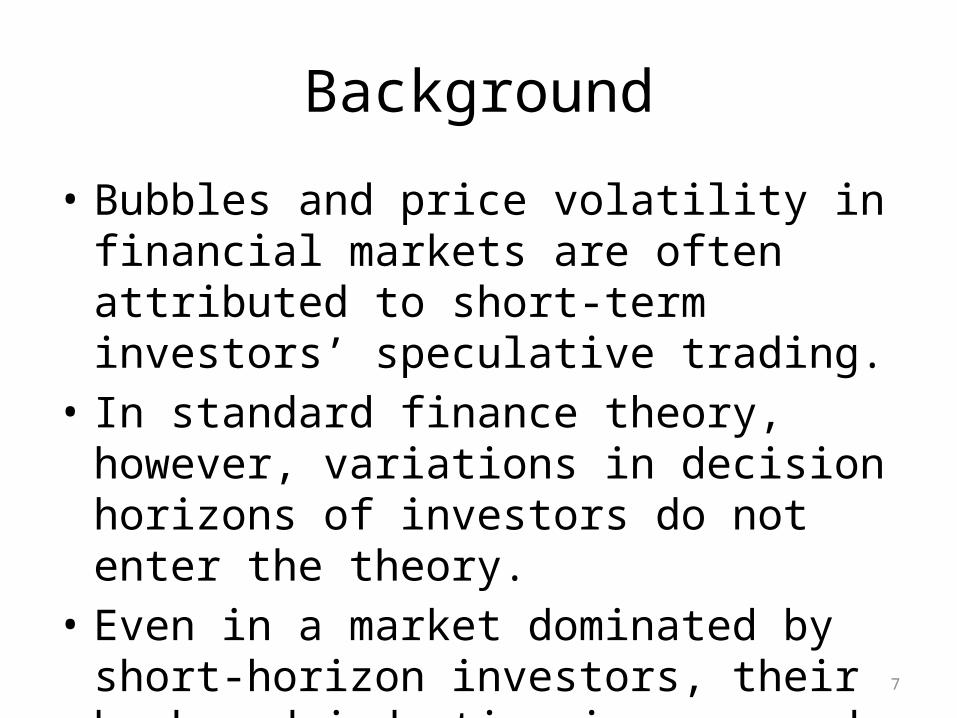
• Bubbles and price volatility in financial markets are often attributed to short-term investors’ speculative trading.

• In standard finance theory, however, variations in decision horizons of investors do not enter the theory.

• Even in a market dominated by short-horizon investors, their backward induction is supposed to lead prices being close to the fundamental values.

8

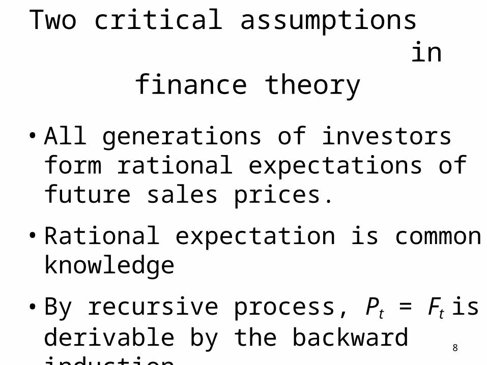
Two critical assumptions in finance theory

• All generations of investors form rational expectations of future sales prices.

• Rational expectation is common knowledge

• By recursive process, Pt = Ft is derivable by the backward induction.

9

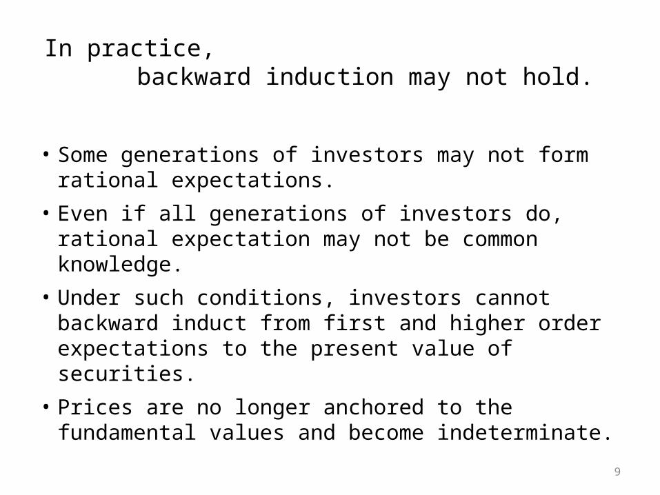
In practice, backward induction may not hold.

• Some generations of investors may not form rational expectations.

• Even if all generations of investors do, rational expectation may not be common knowledge.

• Under such conditions, investors cannot backward induct from first and higher order expectations to the present value of securities.

• Prices are no longer anchored to the fundamental values and become indeterminate.

10

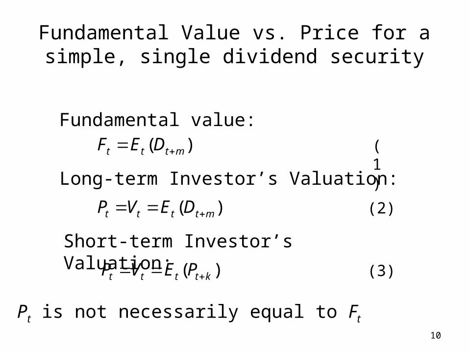
Fundamental Value vs. Price for a simple, single dividend security

Fundamental value:

Long-term Investor’s Valuation:

(1)

(2)

Short-term Investor’s Valuation:

)( mtttt DEVP

)( mttt DEF

)( ktttt PEVP (3)

Pt is not necessarily equal to Ft

11

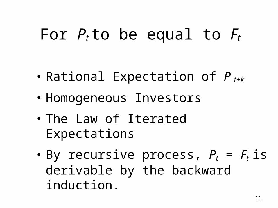
For Pt to be equal to Ft

• Rational Expectation of P t+k

• Homogeneous Investors

• The Law of Iterated Expectations　• By recursive process, Pt = Ft is derivable by

the backward induction.

12

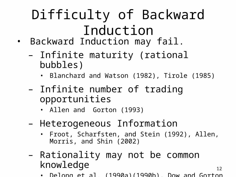
Difficulty of Backward Induction• Backward Induction may fail.

– Infinite maturity (rational bubbles) • Blanchard and Watson (1982), Tirole (1985)

– Infinite number of trading opportunities • Allen and Gorton (1993)

– Heterogeneous Information• Froot, Scharfsten, and Stein (1992), Allen, Morris, and Shin (2002)

– Rationality may not be common knowledge• Delong et al. (1990a)(1990b), Dow and Gorton (1994)

13

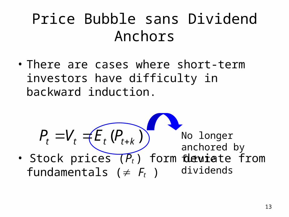
Price Bubble sans Dividend Anchors

• There are cases where short-term investors have difficulty in backward induction.

• Stock prices (Pt ) form deviate from fundamentals ( Ft )

No longer anchored by future dividends

)( ktttt PEVP

14

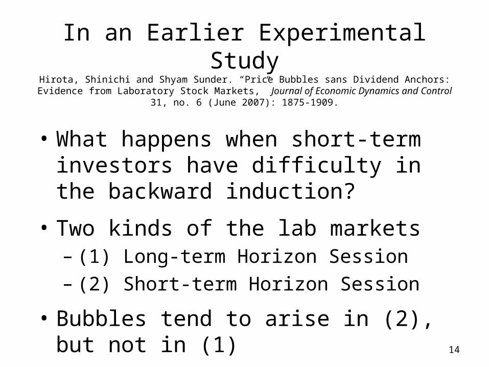
In an Earlier Experimental StudyHirota, Shinichi and Shyam Sunder. “Price Bubbles sans Dividend Anchors: Evidence

from Laboratory Stock Markets,” Journal of Economic Dynamics and Control 31, no. 6 (June 2007): 1875-1909.

• What happens when short-term investors have difficulty in the backward induction?

• Two kinds of the lab markets – (1) Long-term Horizon Session– (2) Short-term Horizon Session

• Bubbles tend to arise in (2), but not in (1)

15

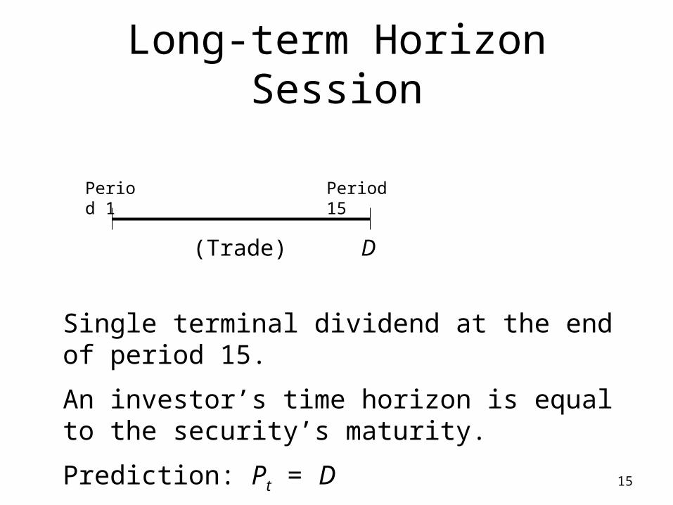
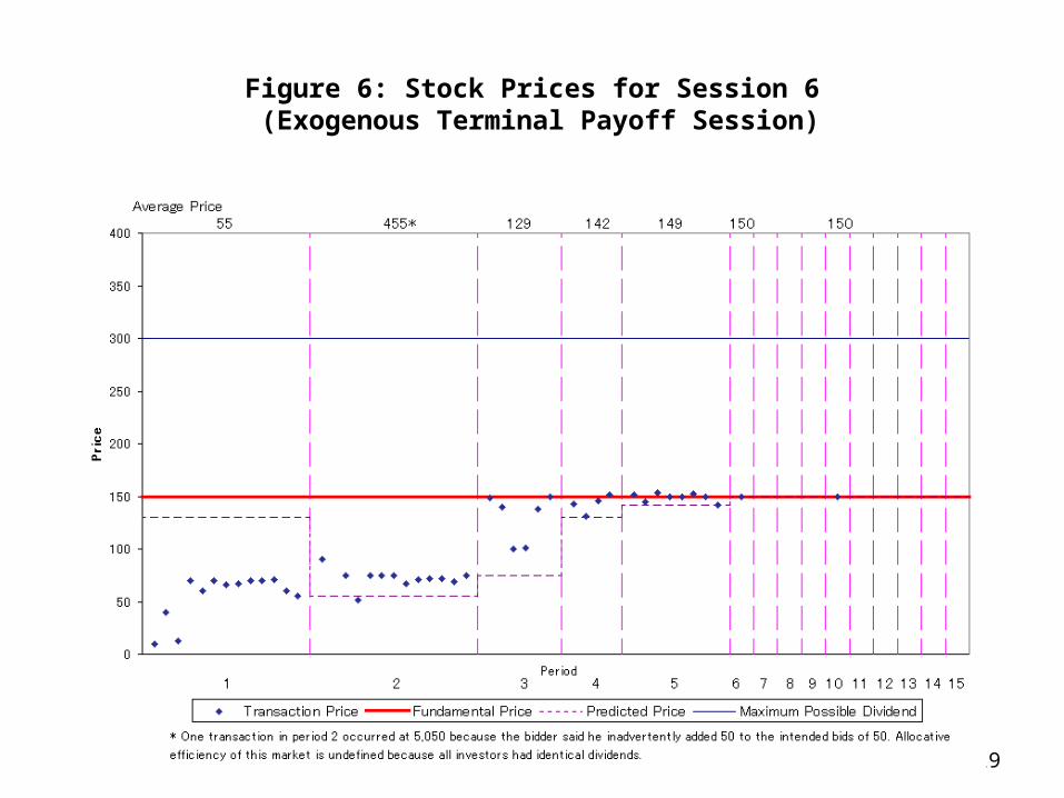
Long-term Horizon Session

Single terminal dividend at the end of period 15.

An investor’s time horizon is equal to the security’s maturity.

Prediction: Pt = D

Period 1 Period 15

D(Trade)

16

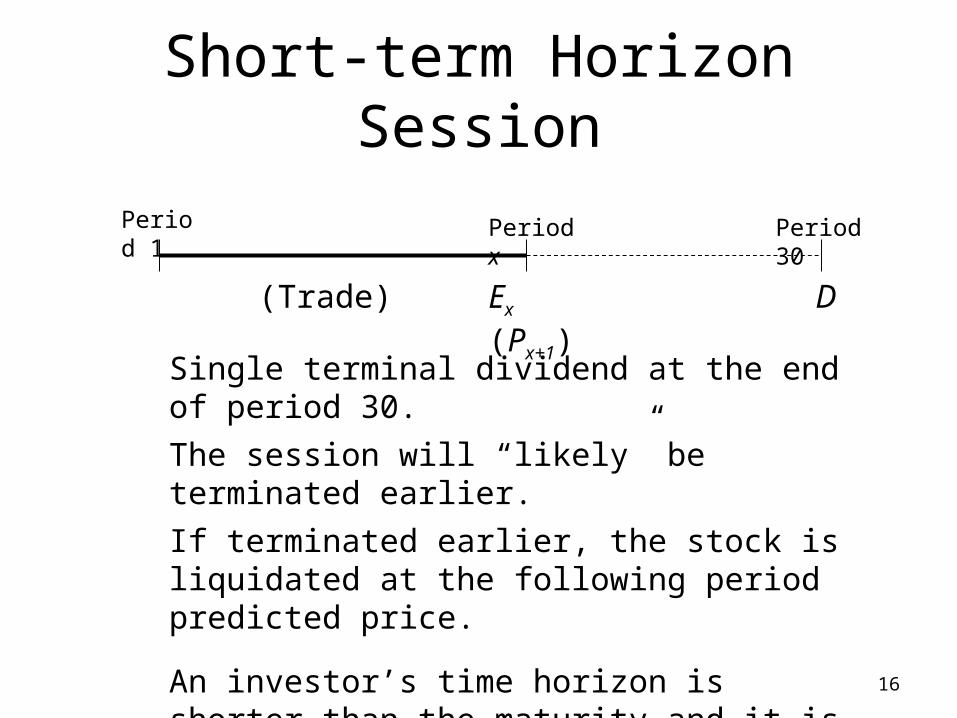
Short-term Horizon Session

Single terminal dividend at the end of period 30.The session will “likely” be terminated earlier. If terminated earlier, the stock is liquidated at the following period predicted price.

An investor’s time horizon is shorter than the maturity and it is difficult to backward induct.Prediction: Pt D

Period 1 Period x Period 30

DEx (Px+1)(Trade)

17

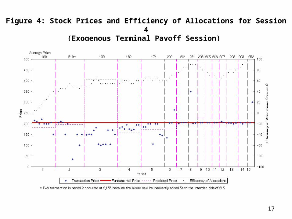
Figure 4: Stock Prices and Efficiency of Allocations for Session 4(Exogenous Terminal Payoff Session)

18

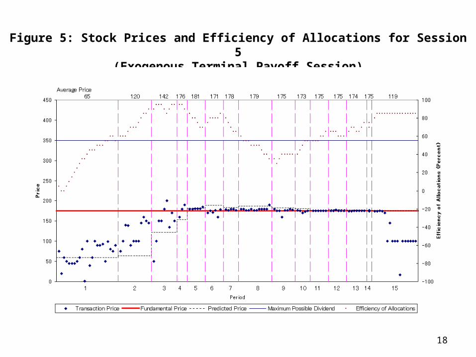
Figure 5: Stock Prices and Efficiency of Allocations for Session 5(Exogenous Terminal Payoff Session)

19

Figure 6: Stock Prices for Session 6 (Exogenous Terminal Payoff Session)

20

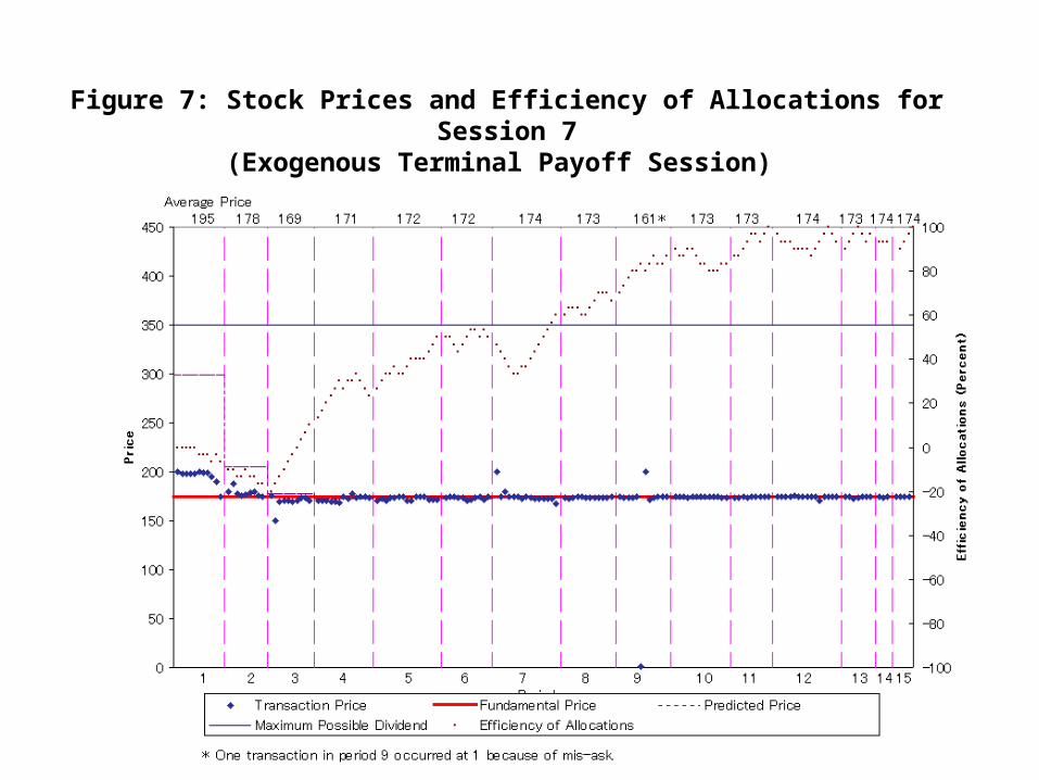
Figure 7: Stock Prices and Efficiency of Allocations for Session 7(Exogenous Terminal Payoff Session)

21

In long-horizon sessions

• Long-horizon Investors play a crucial role in assuring efficient pricing.– Their arbitrage brings prices to the fundamentals.

• Speculative trades do not seem to destabilize prices.– 39.0% of transactions were speculative trades.

• By contrast, in short horizon treatments:

22

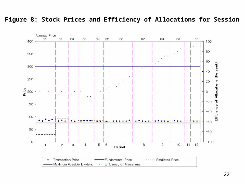
Figure 8: Stock Prices and Efficiency of Allocations for Session 1 (Endogenous Terminal Payoff Session)

23

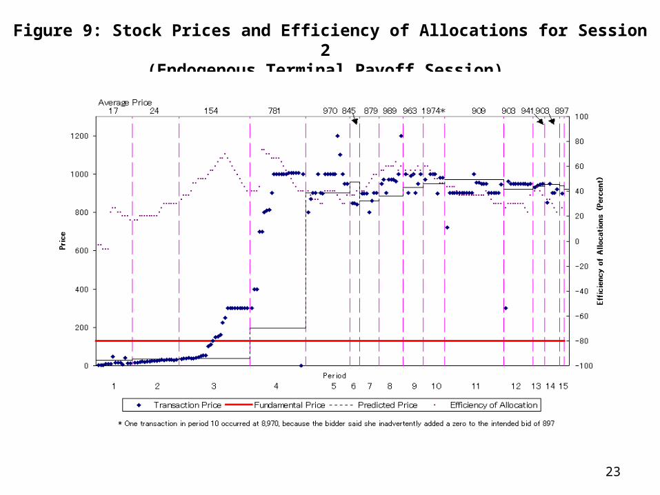
Figure 9: Stock Prices and Efficiency of Allocations for Session 2 (Endogenous Terminal Payoff Session)

24

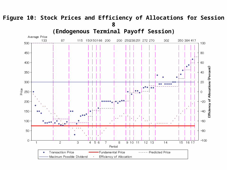
Figure 10: Stock Prices and Efficiency of Allocations for Session 8(Endogenous Terminal Payoff Session)

25

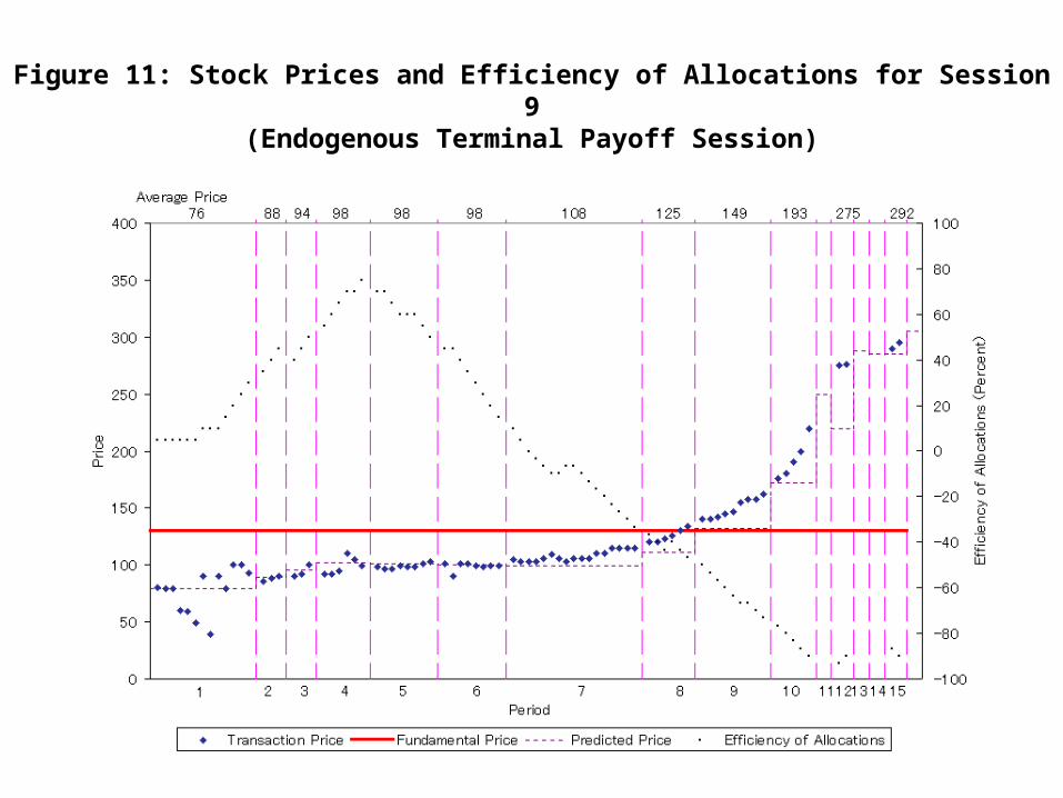
Figure 11: Stock Prices and Efficiency of Allocations for Session 9(Endogenous Terminal Payoff Session)

26

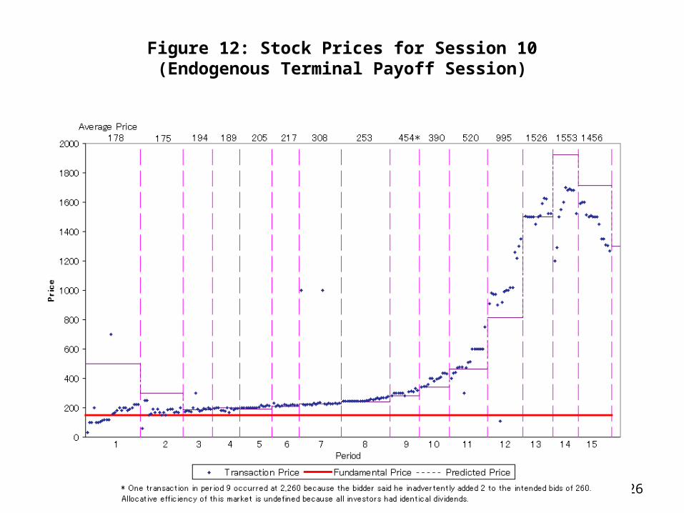
Figure 12: Stock Prices for Session 10(Endogenous Terminal Payoff Session)

27

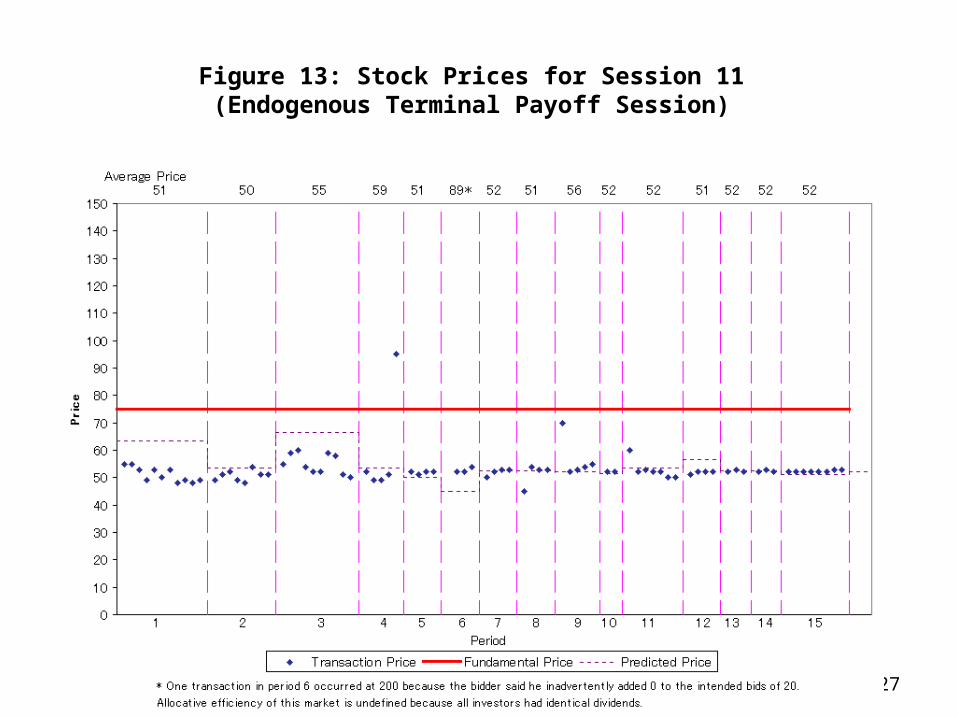
Figure 13: Stock Prices for Session 11 (Endogenous Terminal Payoff Session)

28

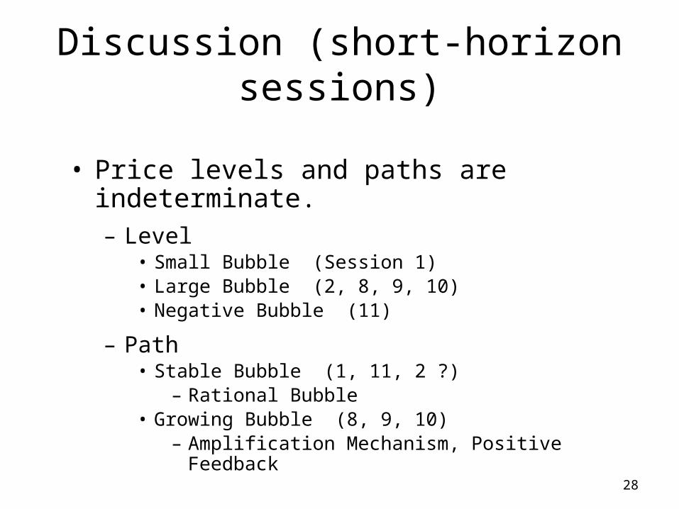
Discussion (short-horizon sessions)

• Price levels and paths are indeterminate.– Level

• Small Bubble (Session 1)• Large Bubble (2, 8, 9, 10)• Negative Bubble (11)

– Path• Stable Bubble (1, 11, 2 ?)

– Rational Bubble• Growing Bubble (8, 9, 10)

– Amplification Mechanism, Positive Feedback

29

Result

• In the long-horizon sessions, price expectations are consistent with backward induction.

• In the short-horizon sessions, price expectations are consistent with forward induction.

30

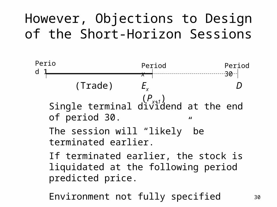
However, Objections to Design of the Short-Horizon Sessions

Single terminal dividend at the end of period 30.The session will “likely” be terminated earlier. If terminated earlier, the stock is liquidated at the following period predicted price.

Environment not fully specified

In the current work, we use a fully specified overlapping generations structure

Period 1 Period x Period 30

DEx (Px+1)(Trade)

31

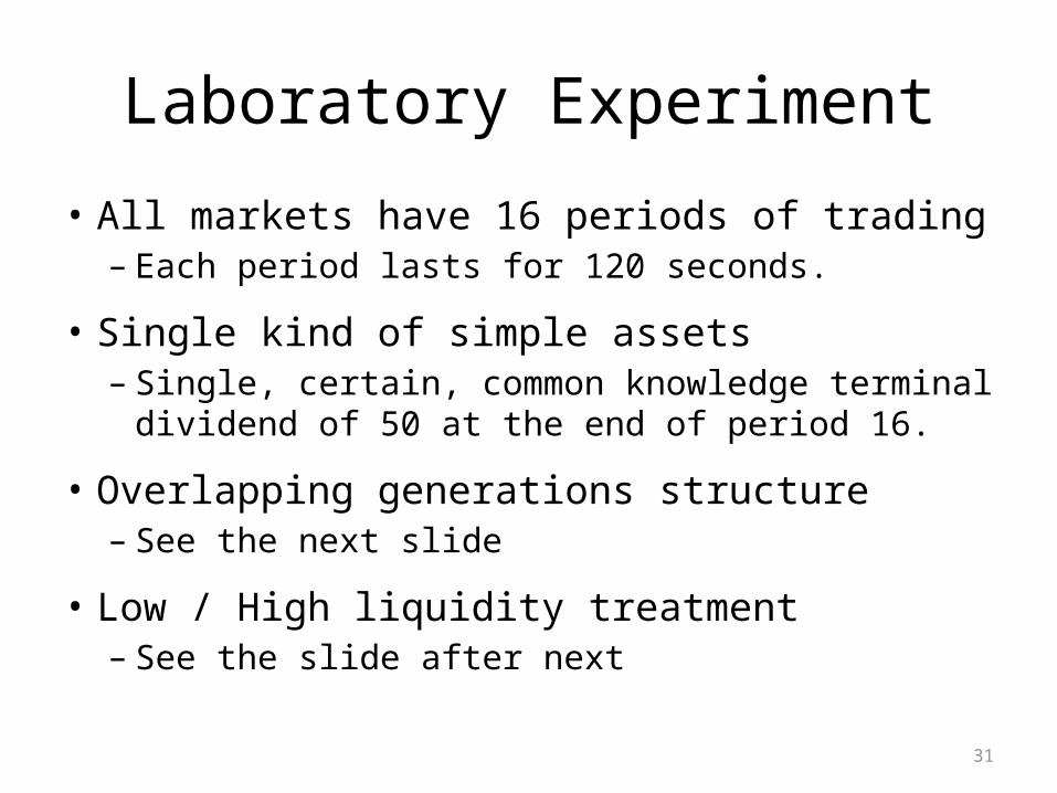
Laboratory Experiment

• All markets have 16 periods of trading– Each period lasts for 120 seconds.

• Single kind of simple assets– Single, certain, common knowledge terminal dividend

of 50 at the end of period 16.

• Overlapping generations structure– See the next slide

• Low / High liquidity treatment– See the slide after next

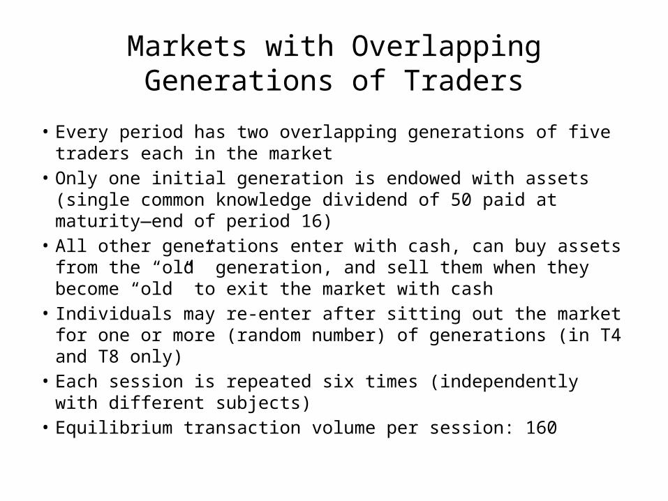
Markets with Overlapping Generations of Traders

• Every period has two overlapping generations of five traders each in the market

• Only one initial generation is endowed with assets (single common knowledge dividend of 50 paid at maturity—end of period 16)

• All other generations enter with cash, can buy assets from the “old” generation, and sell them when they become “old” to exit the market with cash

• Individuals may re-enter after sitting out the market for one or more (random number) of generations (in T4 and T8 only)

• Each session is repeated six times (independently with different subjects)

• Equilibrium transaction volume per session: 160

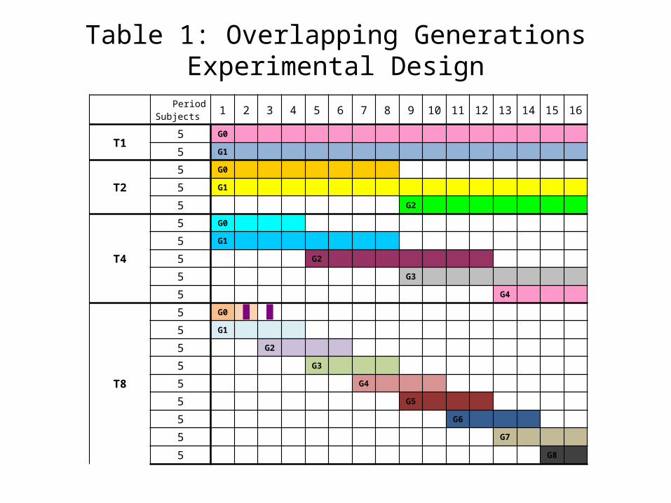
Table 1: Overlapping Generations Experimental Design

  PeriodSubjects 1 2 3 4 5 6 7 8 9 10 11 12 13 14 15 16

T15 G0                              5 G1                              

T25 G0                              5 G1                              5                 G2              

T4

5 G0                              5 G1                              5         G2                      5                 G3              5                         G4      

T8

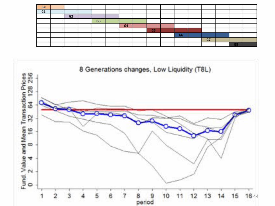
5 G0                              5 G1                              5     G2                          5         G3                      5             G4                  5                 G5              5                     G6          5                         G7      5                             G8  

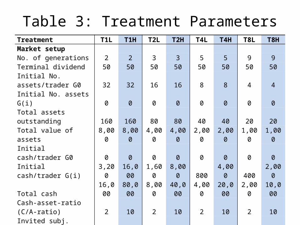
Table 3: Treatment ParametersTreatment T1L T1H T2L T2H T4L T4H T8L T8HMarket setup                No. of generations 2 2 3 3 5 5 9 9Terminal dividend 50 50 50 50 50 50 50 50Initial No. assets/trader G0 32 32 16 16 8 8 4 4Initial No. assets G(i) 0 0 0 0 0 0 0 0Total assets outstanding 160 160 80 80 40 40 20 20Total value of assets 8,000 8,000 4,000 4,000 2,000 2,000 1,000 1,000Initial cash/trader G0 0 0 0 0 0 0 0 0Initial cash/trader G(i) 3,200 16,000 1,600 8,000 800 4,000 400 2,000Total cash 16,000 80,000 8,000 40,000 4,000 20,000 2,000 10,000Cash-asset-ratio (C/A-ratio) 2 10 2 10 2 10 2 10Invited subj. (3n+3) 15a 15a 18 18 18 18 18 18Participating subjects 90 90 108 108 108 108 108 108       Exchange rates (Taler/€)      Generation 0 (G0) 100 100 100 100 100 100 100 100Transition generations   100 500 100 500 100 500Last generation 200 1,000 200 1,000 200 1,000 200 1,000Predictors 133 133 133 133 133 133 133 133Exp. payout/subject (euros) 16 16 16 16 16 16 16 16

NOTES: The following parameters are identical across all treatments: Number of traders/generation (5); number of active generations (2); market size (10 traders); period length (120 sec.); total number of periods (16); number of markets per treatment (6); number of expected transactions (160).a In treatments T1LH we invited 15 subjects instead of 18 as no subject pool for future generations is needed. However we invited five subjects to serve as predictors.

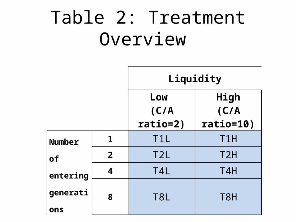
Table 2: Treatment Overview

    Liquidity

    Low (C/A ratio=2)

High(C/A ratio=10)

Number of

entering

generations

1 T1L T1H2 T2L T2H4 T4L T4H8 T8L T8H

36

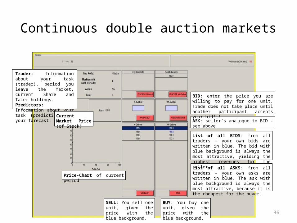
Continuous double auction markets

Trader: Information about your task (trader), period you leave the market, current Share and Taler holdings.Predictors: Information about your task (predictior) and your forecast.

Current Market Price (of Stock)

Price-Chart of current period

SELL: You sell one unit, given the price with the blue background.

BUY: You buy one unit, given the price with the blue background.

List of all ASKS: from all traders - your own asks are written in blue. The ask with blue background is always the most attractive, because it is the cheapest for the buyer.

List of all BIDS: from all traders - your own bids are written in blue. The bid with blue background is always the most attractive, yielding the highest revenues for the seller.

ASK: seller’s analogue to BID - see above.

BID: enter the price you are willing to pay for one unit. Trade does not take place until another participant accepts your bid!!!

37

Conducted Experiments

• Innsbruck-EconLab at University of Innsbruck

• September, October and November 2013

• A total of 828 University of Innsbruck students (bachelor and master from different fields).

38

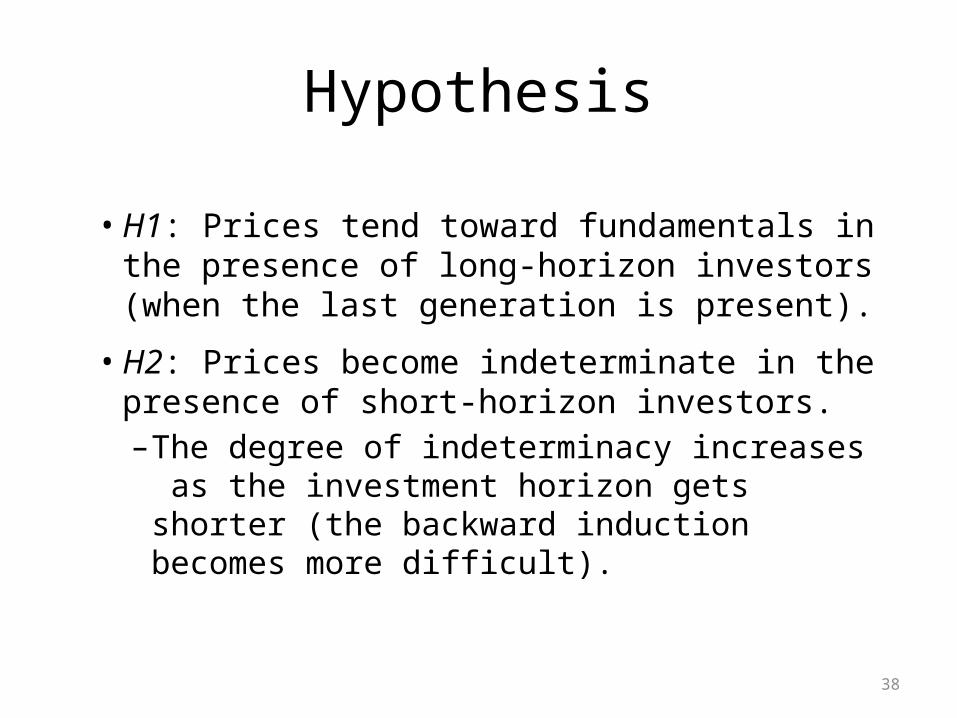
Hypothesis

• H1: Prices tend toward fundamentals in the presence of long-horizon investors (when the last generation is present).

• H2: Prices become indeterminate in the presence of short-horizon investors. – The degree of indeterminacy increases as

the investment horizon gets shorter (the backward induction becomes more difficult).

39

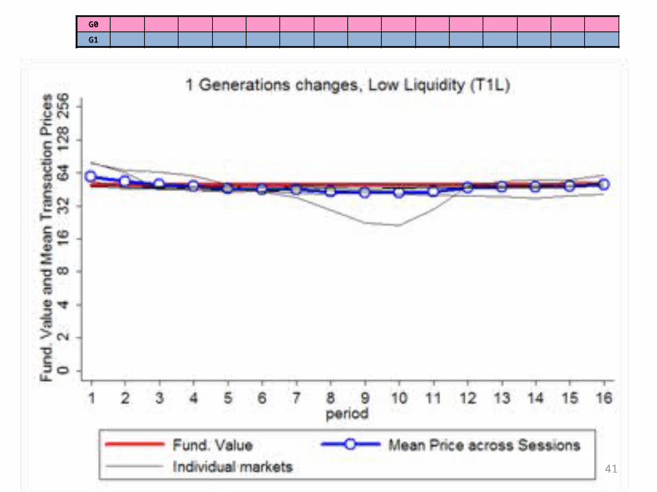
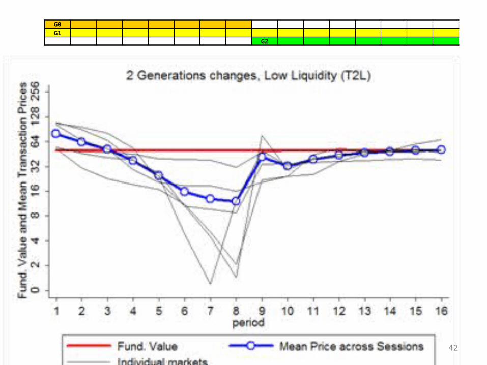
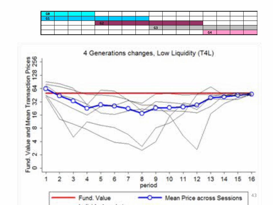
Experimental Results

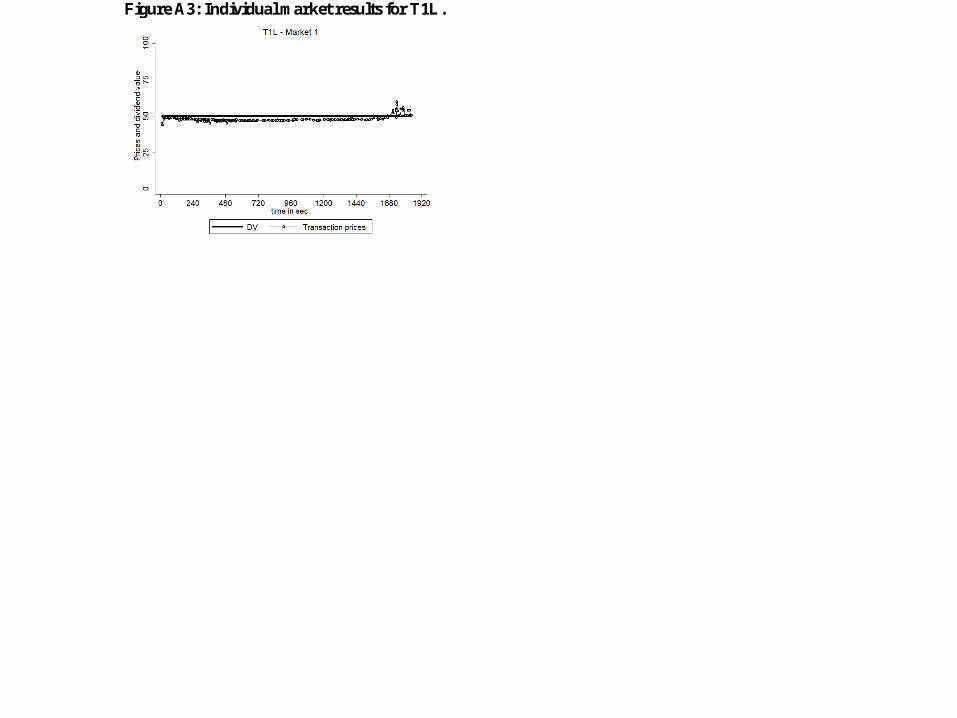
Figure A3: Individual market results for T1L.

41

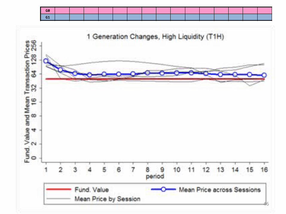
G0

G1

42

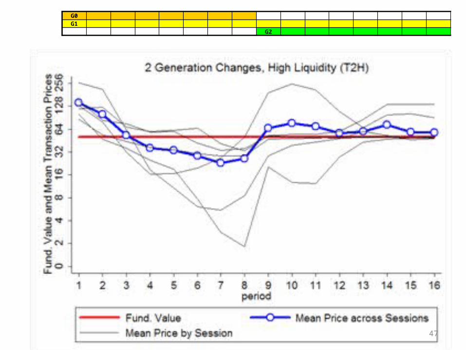
G0G1

G2

43

G0G1

G2G3

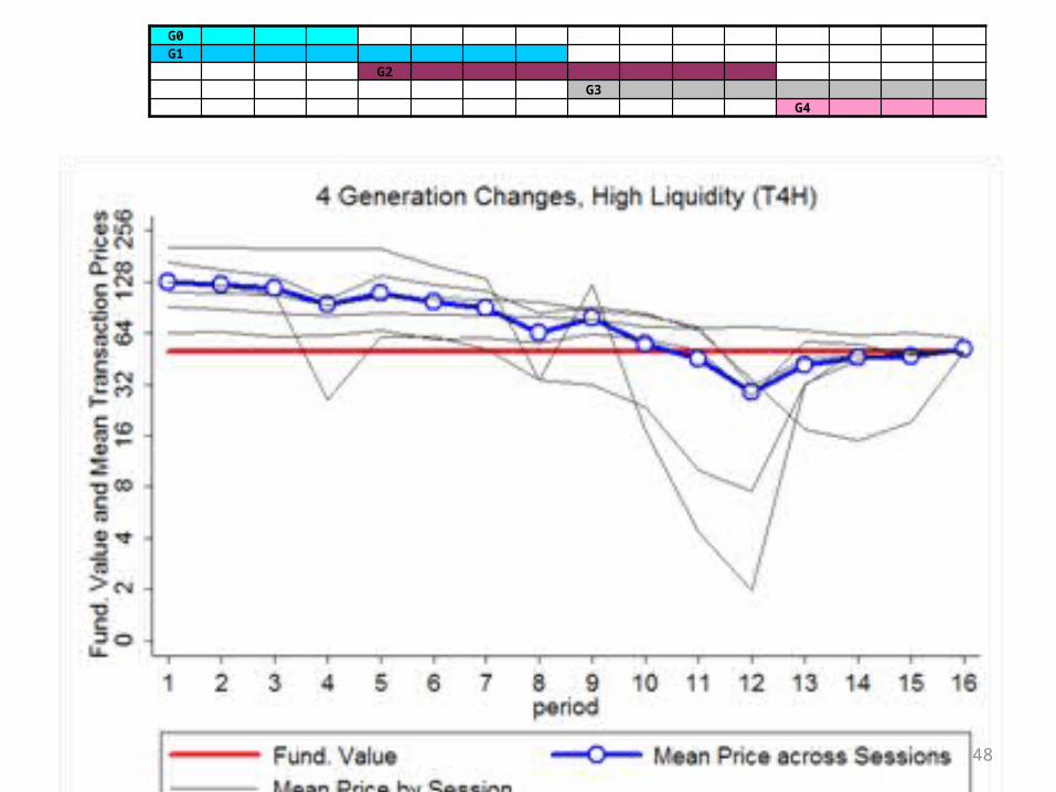
G4

44

G0G1

G2G3

G4G5

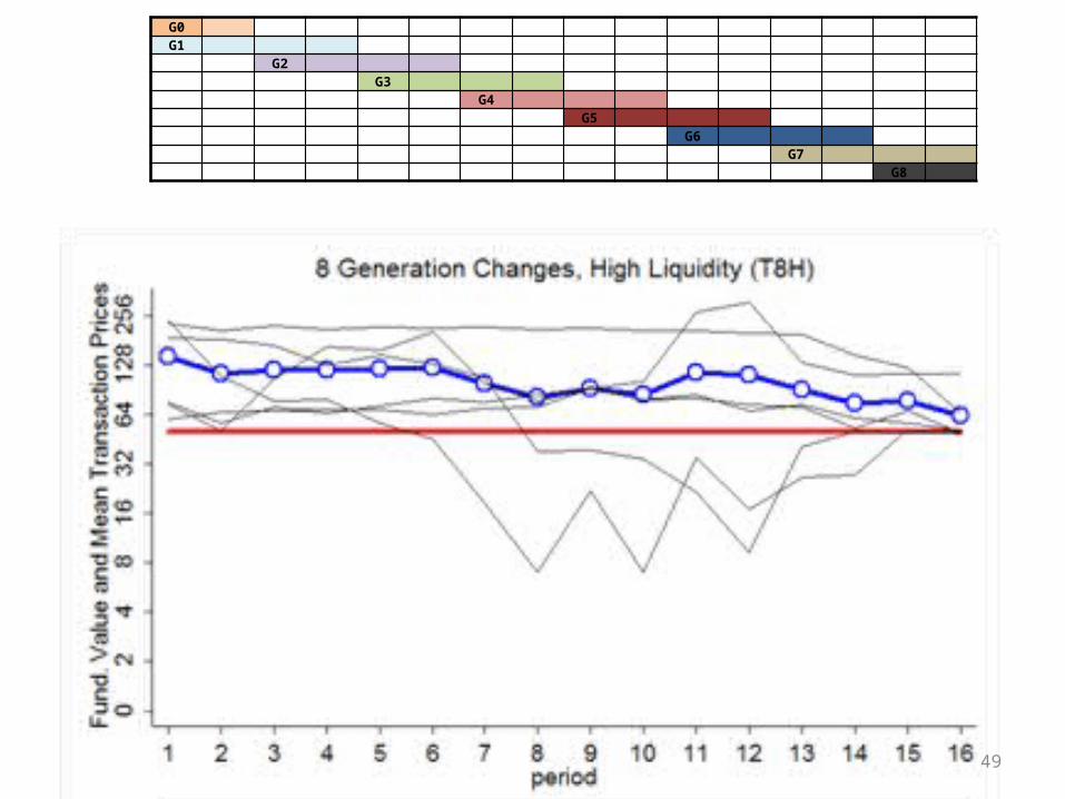
G6G7

G8

45

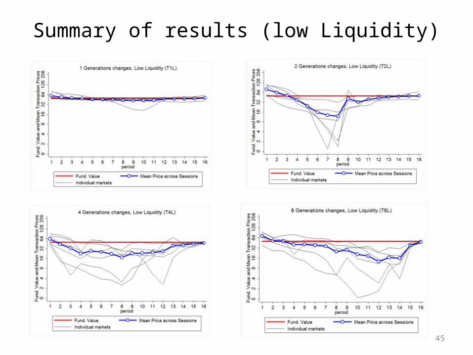
Summary of results (low Liquidity)

46

G0

G1

47

G0G1

G2

48

G0G1

G2G3

G4

49

G0G1

G2G3

G4G5

G6G7

G8

50

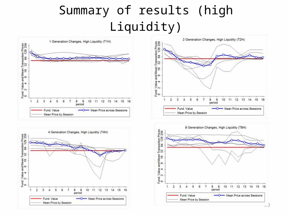
Summary of results (high Liquidity)

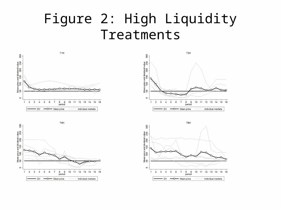
Figure 2: High Liquidity Treatments

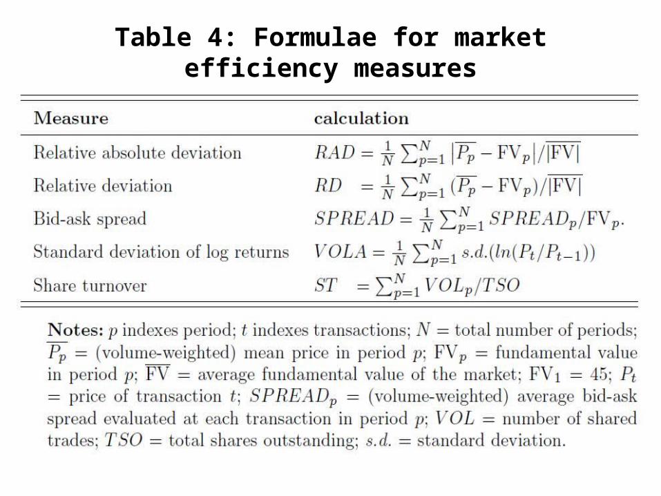
Table 4: Formulae for market efficiency measures

Figure A2: Average absolute prediction error.

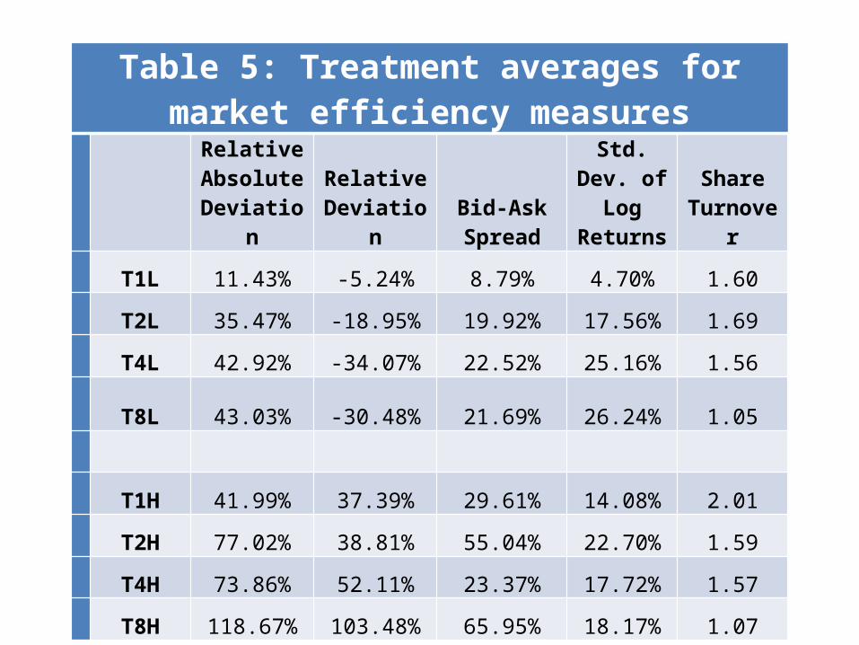
Table 5: Treatment averages for market efficiency measures

Relative Absolute Deviation

Relative Deviation

Bid-Ask Spread

Std. Dev. of Log

ReturnsShare

Turnover T1L 11.43% -5.24% 8.79% 4.70% 1.60 T2L 35.47% -18.95% 19.92% 17.56% 1.69 T4L 42.92% -34.07% 22.52% 25.16% 1.56

T8L 43.03% -30.48% 21.69% 26.24% 1.05

T1H 41.99% 37.39% 29.61% 14.08% 2.01 T2H 77.02% 38.81% 55.04% 22.70% 1.59 T4H 73.86% 52.11% 23.37% 17.72% 1.57 T8H 118.67% 103.48% 65.95% 18.17% 1.07

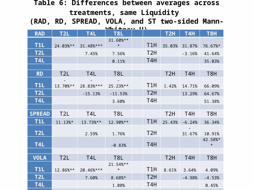
Table 6: Differences between averages across treatments, same Liquidity (RAD, RD, SPREAD, VOLA, and ST two-sided Mann-Whitney U)

RAD T2L T4L T8L T2H T4H T8HT1L 24.03%** 31.48%*** 31.60%*** T1H 35.03% 31.87% 76.67%*T2L 7.45% 7.56% T2H -3.16% 41.64%T4L 0.11% T4H 35.03%

RD T2L T4L T8L T2H T4H T8HT1L -13.70%** -28.83%*** -25.23%** T1H 1.42% 14.71% 66.09%T2L -15.13% -11.53% T2H 13.29% 64.67%T4L 3.60% T4H 51.38%

SPREAD T2L T4L T8L T2H T4H T8HT1L 11.13%* 13.73%** 12.90%** T1H 25.43% -6.24% 36.34%T2L 2.59% 1.76% T2H -31.67% 10.91%T4L -0.83% T4H 42.58%**

VOLA T2L T4L T8L T2H T4H T8HT1L 12.86%** 20.46%*** 21.54%*** T1H 8.61% 3.64% 4.09%T2L 7.60% 8.68%* T2H -4.98% -4.53%T4L 1.08% T4H 0.45%

ST T2L T4L T8L T2H T4H T8HT1L 0.09 -0.03 -0.55** T1H -0.43 -0.44 -0.94**T2L -0.12 -0.64*** T2H -0.02 -0.52**T4L -0.51 T4H -0.50**

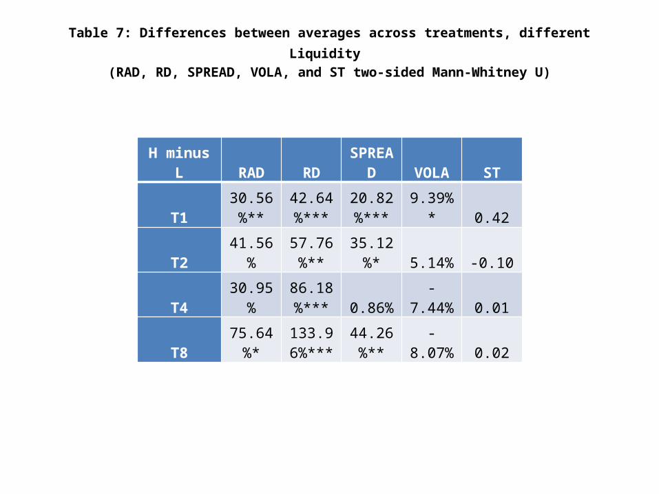
Table 7: Differences between averages across treatments, different Liquidity (RAD, RD, SPREAD, VOLA, and ST two-sided Mann-Whitney U)

H minus L RAD RD SPREAD VOLA ST

T130.56%

**42.64%

***20.82%

*** 9.39%* 0.42

T2 41.56%57.76%

**35.12%

* 5.14% -0.10

T4 30.95%86.18%

*** 0.86% -7.44% 0.01

T875.64%

*133.96%***

44.26%** -8.07% 0.02

Price Predictions/Expectations• Not yet analyzed for the current study• Hirota and Sunder (2007): results show that when subjects

cannot do backward induction, they resort to forward induction, and simply project past data in forming their expectations about the future

• In long-horizon sessions, future price expectations are formed by fundamentals.

– Speculation stabilizes prices.

• In short-term sessions, future price expectations are formed by their own or actual prices.– Speculation may destabilize prices.

58

Wrap Up• Prices are close to the fundamental values when Investors

have long-term horizons.

• Prices deviate from the fundamental values and become indeterminate when there are only short-term investors in the market. – Investors fail to backward induct to bring prices to the

fundamental values.– The shorter the investment horizon (the larger number of

generations), the more difficult the backward induction.– Prices in high liquidity treatments are higher and deviate more

from fundamentals than those in low liquidity treatments.

Implications• Bubbles are known to occur more often in markets for

assets with – (i) longer maturity and duration– (ii) higher uncertainty

• Consistent with the lab data• Inputs to expectation formation matter:

– Dividend policy matters!• Ex post, market inefficiency, anomalies, and behavioral

phenomena more likely to be observed in markets dominated by short-horizon investors (difficulty of backward induction)

Thank You!

Shyam.sunder@yale.eduhttp://faculty.som.yale.edu/shyamsunder/research.html