Ship-Hull Shape Optimization with a T-spline basedBEM-Isogeometric Solver

K.V. Kostasa,∗, A.I. Ginnisb, C.G. Politisa, P.D. Kaklisc

aDepartment of Naval Architecture, Technological Educational Institute of AthensbSchool of Naval Architecture & Marine Engineering, National Technical University of AthenscDepartment of Naval Architecture, Ocean and Marine Engineering, University of Strathclyde

Abstract

In this work, we present a ship-hull optimization process combining a T-spline based parametric

ship-hull model and an Isogeometric Analysis (IGA) hydrodynamic solver for the calculation of

ship wave resistance. The surface representation of the ship-hull instances comprise one cubic

T-spline with extraordinary points, ensuring C2 continuity everywhere except for the vicinity of

extraordinary points where G1 continuity is achieved. The employed solver for ship wave resistance

is based on the Neumann-Kelvin formulation of the problem, where the resulting Boundary In-

tegral Equation is numerically solved using a higher order collocated Boundary Element Method

which adopts the IGA concept and the T-spline representation for the ship-hull surface. The

hydrodynamic solver along with the ship parametric model are subsequently integrated within

an appropriate optimization environment for local and global ship-hull optimizations against the

criterion of minimum resistance.

1. INTRODUCTION

Due to an increasing demand for efficiency and robustness in Computer Aided Ship Design

(CASD), the available modeling, analysis and evaluation techniques are being continuously pushed

forward so that they can provide measurable improvements for both the design process and the

resulting product. Fortunately, the current availability of computing power has allowed the em-

ployment of sophisticated Computational Fluid Dynamic (CFD) solvers and their coupling with

advanced Geometric Modeling techniques and Optimization strategies, a combination that offers

significant aid to meet the demanding requirements of contemporary CASD.

The optimization of a hull-form with respect to its resistance and resulting fuel consumption has

always been a major task in ship design. Moreover, as the design of the hull form is a prerequisite

for the majority of ship design tasks, it is of great importance to complete this task in the earliest

possible time. The present work is focused in developing an appropriate ship-hull hydrodynamic

∗Corresponding author: kvkostas@teiath.gr

Preprint submitted to Elsevier October 12, 2014

optimization process, combining modern optimization techniques, a fully parametric T-spline ship-

hull model and a BEM hydrodynamic solver. Both the parametric model and hydrodynamic solver

are in-house developed. Note that the hydrodynamic solver adopts the concept of Isogeometric

Analysis (IGA), introduced by Hughes et al. [1], which aims to intrinsically integrate CAD with

Analysis by communicating the CAD model of the geometry (ship hull) to the solver without any

approximation, e.g., panelization. Furthermore, Basilevs et al [2] and Scott et al [3] have already

demonstrated the efficient usage of IGA in conjunction with T-splines technology [4, 5]. Shape

optimization, in the context of IGA, has been presented in various works as, e.g., in [6, 7, 8] for

the 2D case and in [9] for the 3D case. In these works, the control points are directly used as

shape optimization parameters. In our case, due to the shape complexity and restrictions of the

ship-hull, we have developed a parametric model that uses high-level parameters with physical

meaning for the generation of ship instances. Thus, the control points of the underlying surface

representation are indirectly controlled by these parameters.

The methodology for constructing the parametric ship-hull model is presented in Section 2.

The method is materialized within the Rhinocerosr[10] modeling environment, with the aid of its

scripting functionality and Autodeskr’s T-Splinesr Plug-In [11] for Rhinocerosr. It should be

noted that the functionality of parametric modeling is not offered by the above software tools; it is

in-house developed using the Rhinoscripting programming language. An early attempt for building

a ship parametric model is due to Lackenby [12] in which hull variants are obtained by modifying

the prismatic coefficient, the center of buoyancy and the extent and position of parallel mid-body

of a parent hull. This method has been subsequently generalized towards improving the geometric

coverage of the parametric model through the use of B-spline techniques; see, e.g., Harries and

Nowacki [13], Kim [14], Abt and Harries [15], Harries [16] and Ping [17]. In previous works of

ours [18, 19], a Ship Parametric Model (SPM) has been developed, with the aid of CATIAr[20]

modeling environment, resulting in a multi-patch NURBS representation of a ship hull. This

methodology initiated with a list of exposed and internal parameters, which were devised on the

basis of parent hulls and proceeded with the generation of control curve networks, appropriately

augmented with corresponding cross-tangent ribbons. The ship-surface construction was thus

reduced to a sequence of local Hermite interpolation problems which were solved through CATIA

tools, yielding a tangentially-continuous (G1) NURBS multi-patch representation of the ship hull.

In this work, in order to remove deficiencies due to the multi-patch NURBS representation, see [21,

22, 23], we use the T-splines technology, for the construction of the SPM. The methodology initiates

again with a list of exposed and internals parameters, extracted from the form of parent ships. Both

types of parameters are used to parametrically construct the Control Cage, which determines the

topology of the unstructured T-mesh and acts as the control “polyhedron” for the generated cubic

T-spline surface. This construction uses Autodeskr’s T-Splinesr Plug-In functionality to produce

2

an analysis suitable T-spline mesh for the ship-hull surface. The produced surface is of higher

smoothness (C2 continuity) compared to its corresponding NURBS multi-patch representation

(G1 continuity), except in the vicinity of the extraordinary points, where G1 continuity is achieved;

see [3].

Section 3 is devoted to the presentation of the CFD solver’s basic features. The CFD wave

resistance solver is based on the Neumann-Kelvin formulation of the problem, introduced by

Brard [24]; see also [25]. The resulting BIE is numerically solved using a higher order collocated

BEM, which adopts the IGA concept. The analysis suitable T-Spline representation along with

the calculation of collocation points is offered through the IGA export functionality of the T-Spline

Plug-In; see [26]. The in-house developed T-spline based IGA-BEM solver is presented in detail

and tested in [21].

Section 4 presents the optimization environment integrating the SPM, the T-spline based

IGA-BEM solver and the optimization libraries of modeFrontierr[27] for designing ship hulls with

minimum resistance. Finally, two optimization cases (local/global) for a container ship are set-up

and presented in Section 5. The first case deals with bulbous bow optimization (local optimization

problem) against the criterion of minimum wave resistance under a given displacement, while the

second case involves a global ship-hull minimization problem against two objective functions: total

resistance and deviation from a reference ship capacity, i.e., ship’s deadweight.

2. The T-spline Ship Parametric Model (SPM)

In this section, we describe a methodology for constructing a parametric model for typical

ship-hull forms constructed within the Rhinocerosr modeling environment with the aid of its

scripting functionality and Autodeskr’s T-Splinesr Plug-In for Rhinocerosr. Rhinoceros is a

generic NURBS based surface and solid modeler, providing a wide range of functionalities. The

T-Spline plug-in adds T-spline support to Rhinoceros which, with the aid of Rhinoscripting, en-

ables the materialization of the methodology for generating a T-spline ship-hull parametric model.

Finally, the automation offered in Rhinoceros through various scripting languages can easily con-

stitute the developing framework for the creation of the wrapper required in the optimization

process; see §4,5.

The basic shape characteristics of a typical ship-hull comprise:

• a partition of the ship-hull into three main parts, namely the bow, the midship part and the

stern,

• global dimensions (e.g., length between perpendiculars (Lbp), beam (B), depth (D), draft

(T)) as well as dimensions characterizing each one of the aforementioned ship parts (e.g.,

extent of the midship part),

3

• a set of control curves that are of boundary (e.g., stern profile, bow profile) or shape-

transition character (e.g., FoS (flat-of-side) and FoB (flat-of-bottom) curves) and, finally,

• local geometrical characteristics that serve functional, structural and/or hydrodynamic pur-

poses, e.g., bow-angle of entrance at waterline, bulb-top position, bilge radius, shaft height,

etc.

On the basis of the above coarse shape description and a set of parent ship-hulls, a list of

exposed and internal parameters is devised. Exposed parameters will be accessible from the

outside of the parametric modeling tool and initiate the modeling process, leading eventually to

the production of a corresponding hull instance. On the contrary, internal parameters are not

visible from the outside of the parametric tool and are used to control the surface construction

process and eventually retain the basic shape characteristics of the parent hulls. Default values

for both exposed and internal parameters are extracted from the parent ships. Furthermore,

a domain of variation is assigned to each parameter assuring the modeling robustness while at

the same time avoiding invalid geometrical models (e.g., self-intersections). These ranges can be

thought as confidence intervals and have to be defined through extensive experimentation with

the parametric model. Finally, SPM favors the use of non-dimensional parameters where possible,

in order to avoid the interdependency between them. Exposed parameters are categorized in four

groups, according to whether they are global, associated to the midship, bow and stern areas of

the ship. Parameters belonging to the global group correspond to ship’s principal dimensions and

their effect is of global nature, e.g., Lwl, B, T; see Fig. 1. The second category includes parameters

that are involved in the generation of the mid-ship part of the ship, e.g., Mid L, Mid Pos; see again

Fig. 1. Although not being global in nature, the effect of these parameters is global as the mid-ship

part is both the initial and supporting entity in the construction of the hull parametric model. The

remaining two categories correspond to the bow and stern parts of the ship and are of more local

character as they define shape forms in the areas of the bow and stern, respectively, see Fig. 2.

The total number of exposed parameters is 24 and are split as follows: 3 global, 9 for the midship

and 7,5 for the bow and stern parts respectively. Both exposed and internal parameters are used

to parametrically construct the Control Cage, which essentially determines the topology of the

T-mesh and acts as the control “polyhedron” for the generated T-spline surface. Specifically, the

Control Cage is the T-mesh for a cubic T-Spline, excluding the outer ring of faces that define the

boundary conditions.

The Control Cage is uniquely defined by the connectivity and position of its vertices. The

connectivity is ship-type dependent and defines the topology. On the other hand, the coordinates

of the vertices are parameter dependent and along with the corresponding topology define the final

hull-shape. Specifically, if X denotes the vector of parameters with X ∈ Rm, m being the total

4

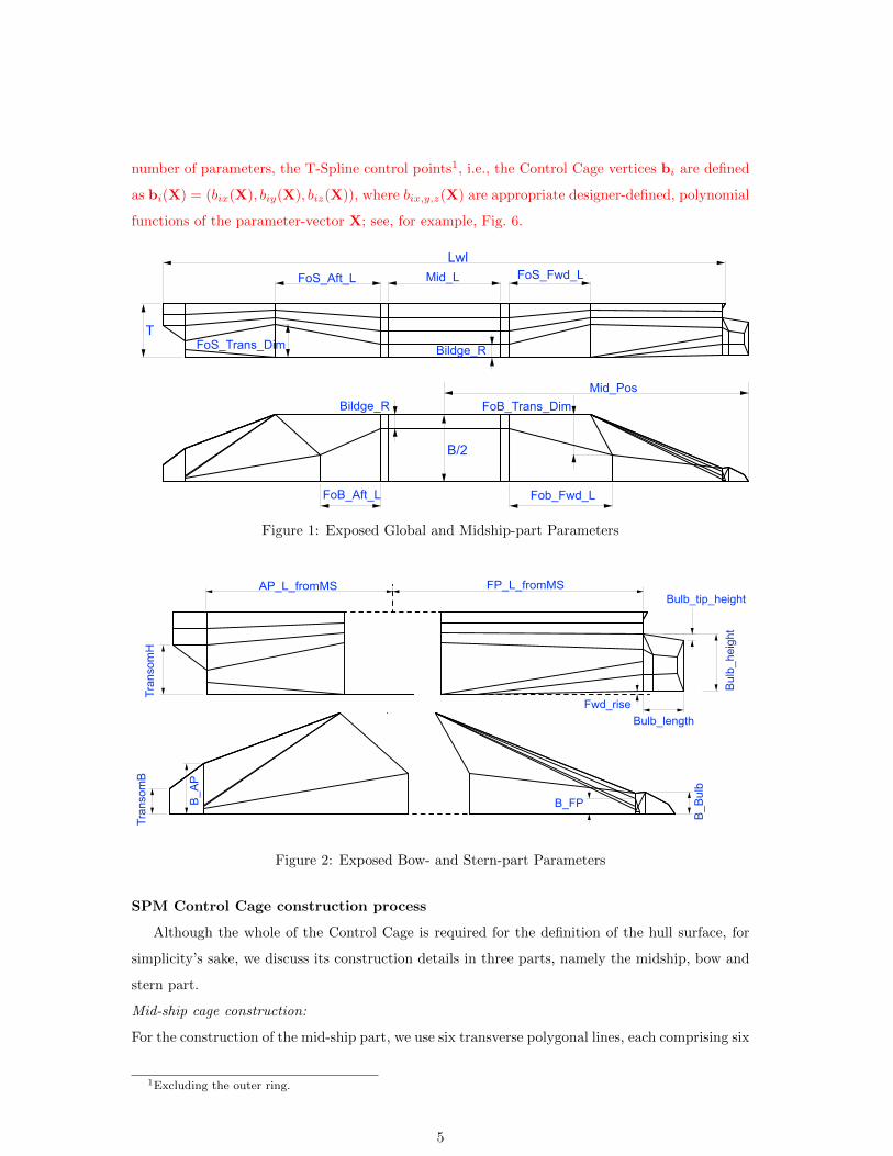
number of parameters, the T-Spline control points1, i.e., the Control Cage vertices bi are defined

as bi(X) = (bix(X), biy(X), biz(X)), where bix,y,z(X) are appropriate designer-defined, polynomial

functions of the parameter-vector X; see, for example, Fig. 6.

Mid_Pos

FoB_Aft_L Fob_Fwd_L

FoB_Trans_Dim

Mid_LFoS_Aft_L FoS_Fwd_L

FoS_Trans_Dim Bildge_R

Bildge_R

Lwl

B/2

T

Figure 1: Exposed Global and Midship-part Parameters

Tran

som

H

Fwd_rise

Bulb_tip_height

Bulb_lengthB

ulb_

heig

ht

AP_L_fromMS FP_L_fromMS

Tran

som

B

B_FPB_A

P

B_B

ulb

Figure 2: Exposed Bow- and Stern-part Parameters

SPM Control Cage construction process

Although the whole of the Control Cage is required for the definition of the hull surface, for

simplicity’s sake, we discuss its construction details in three parts, namely the midship, bow and

stern part.

Mid-ship cage construction:

For the construction of the mid-ship part, we use six transverse polygonal lines, each comprising six

1Excluding the outer ring.

5

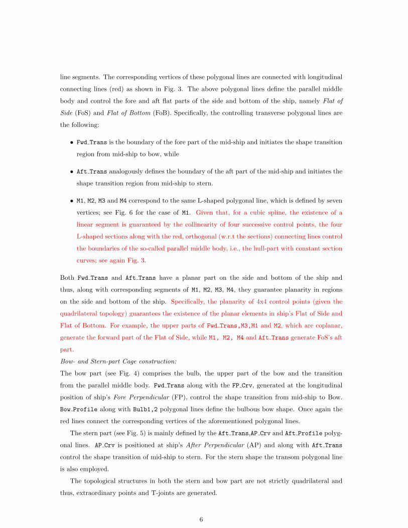
line segments. The corresponding vertices of these polygonal lines are connected with longitudinal

connecting lines (red) as shown in Fig. 3. The above polygonal lines define the parallel middle

body and control the fore and aft flat parts of the side and bottom of the ship, namely Flat of

Side (FoS) and Flat of Bottom (FoB). Specifically, the controlling transverse polygonal lines are

the following:

• Fwd Trans is the boundary of the fore part of the mid-ship and initiates the shape transition

region from mid-ship to bow, while

• Aft Trans analogously defines the boundary of the aft part of the mid-ship and initiates the

shape transition region from mid-ship to stern.

• M1, M2, M3 and M4 correspond to the same L-shaped polygonal line, which is defined by seven

vertices; see Fig. 6 for the case of M1. Given that, for a cubic spline, the existence of a

linear segment is guaranteed by the collinearity of four successive control points, the four

L-shaped sections along with the red, orthogonal (w.r.t the sections) connecting lines control

the boundaries of the so-called parallel middle body, i.e., the hull-part with constant section

curves; see again Fig. 3.

Both Fwd Trans and Aft Trans have a planar part on the side and bottom of the ship and

thus, along with corresponding segments of M1, M2, M3, M4, they guarantee planarity in regions

on the side and bottom of the ship. Specifically, the planarity of 4x4 control points (given the

quadrilateral topology) guarantees the existence of the planar elements in ship’s Flat of Side and

Flat of Bottom. For example, the upper parts of Fwd Trans,M3,M1 and M2, which are coplanar,

generate the forward part of the Flat of Side, while M1, M2, M4 and Aft Trans generate FoS’s aft

part.

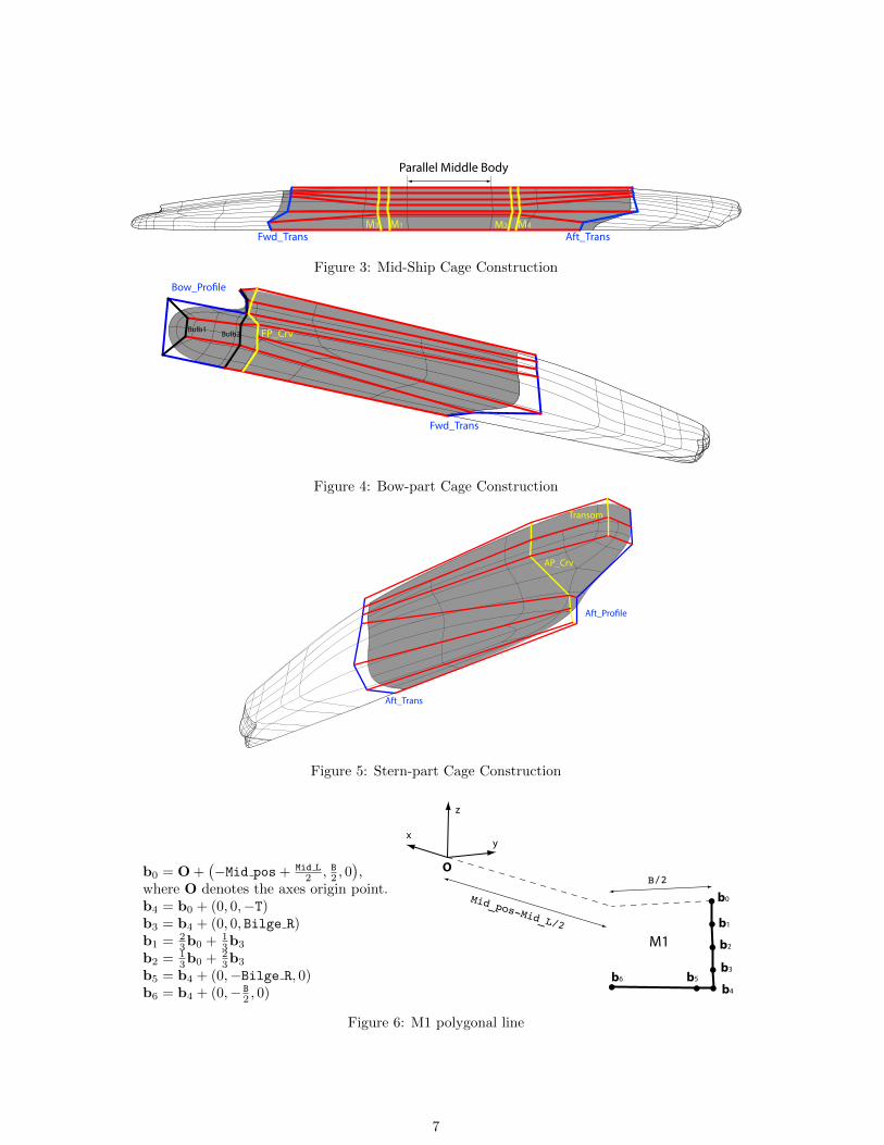
Bow- and Stern-part Cage construction:

The bow part (see Fig. 4) comprises the bulb, the upper part of the bow and the transition

from the parallel middle body. Fwd Trans along with the FP Crv, generated at the longitudinal

position of ship’s Fore Perpendicular (FP), control the shape transition from mid-ship to Bow.

Bow Profile along with Bulb1,2 polygonal lines define the bulbous bow shape. Once again the

red lines connect the corresponding vertices of the aforementioned polygonal lines.

The stern part (see Fig. 5) is mainly defined by the Aft Trans,AP Crv and Aft Profile polyg-

onal lines. AP Crv is positioned at ship’s After Perpendicular (AP) and along with Aft Trans

control the shape transition of mid-ship to stern. For the stern shape the transom polygonal line

is also employed.

The topological structures in both the stern and bow part are not strictly quadrilateral and

thus, extraordinary points and T-joints are generated.

6

M1 M2 M4M3

Fwd_Trans Aft_Trans

Parallel Middle Body

Figure 3: Mid-Ship Cage Construction

Fwd_Trans

Bow_Prole

FP_CrvBulb1Bulb2

Figure 4: Bow-part Cage Construction

Aft_Trans

Aft_Prole

AP_Crv

Transom

Figure 5: Stern-part Cage Construction

b0 = O +(−Mid pos + Mid L

2 , B2 , 0),

where O denotes the axes origin point.b4 = b0 + (0, 0,−T)b3 = b4 + (0, 0, Bilge R)b1 = 2

3b0 + 13b3

b2 = 13b0 + 2

3b3

b5 = b4 + (0,−Bilge R, 0)b6 = b4 + (0,− B

2 , 0)

b0

b1

b2

b3

b4

b5b6

O

xy

z

M1

Mid_pos-Mid_L/2

B/2

Figure 6: M1 polygonal line

7

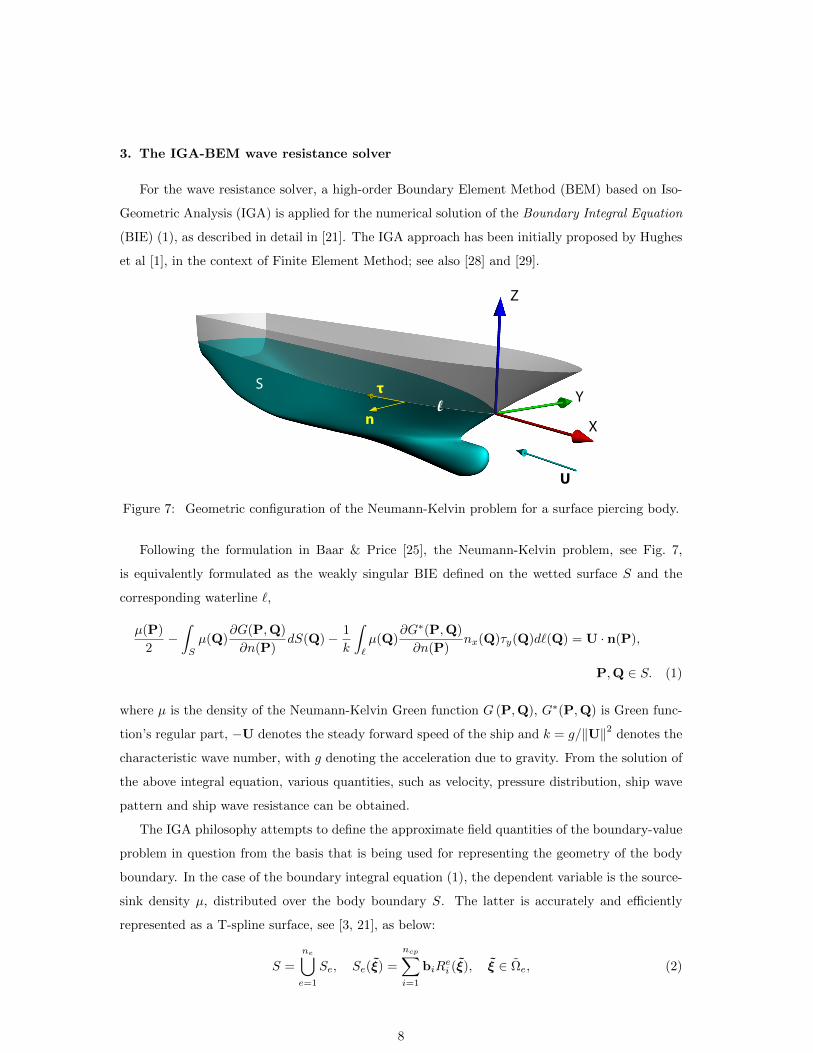
3. The IGA-BEM wave resistance solver

For the wave resistance solver, a high-order Boundary Element Method (BEM) based on Iso-

Geometric Analysis (IGA) is applied for the numerical solution of the Boundary Integral Equation

(BIE) (1), as described in detail in [21]. The IGA approach has been initially proposed by Hughes

et al [1], in the context of Finite Element Method; see also [28] and [29].

Z

X

Y

U

n

τSl

Figure 7: Geometric configuration of the Neumann-Kelvin problem for a surface piercing body.

Following the formulation in Baar & Price [25], the Neumann-Kelvin problem, see Fig. 7,

is equivalently formulated as the weakly singular BIE defined on the wetted surface S and the

corresponding waterline `,

µ(P)

2−∫S

µ(Q)∂G(P,Q)

∂n(P)dS(Q)− 1

k

∫`

µ(Q)∂G∗(P,Q)

∂n(P)nx(Q)τy(Q)d`(Q) = U · n(P),

P,Q ∈ S. (1)

where µ is the density of the Neumann-Kelvin Green function G (P,Q), G∗(P,Q) is Green func-

tion’s regular part, −U denotes the steady forward speed of the ship and k = g/‖U‖2 denotes the

characteristic wave number, with g denoting the acceleration due to gravity. From the solution of

the above integral equation, various quantities, such as velocity, pressure distribution, ship wave

pattern and ship wave resistance can be obtained.

The IGA philosophy attempts to define the approximate field quantities of the boundary-value

problem in question from the basis that is being used for representing the geometry of the body

boundary. In the case of the boundary integral equation (1), the dependent variable is the source-

sink density µ, distributed over the body boundary S. The latter is accurately and efficiently

represented as a T-spline surface, see [3, 21], as below:

S =

ne⋃e=1

Se, Se(ξ) =

ncp∑i=1

biRei (ξ), ξ ∈ Ωe, (2)

8

where ncp is the number of control points, or T-mesh vertices, bi in the T-mesh, Ωe is the

parametric domain of the element e, Rei is the restriction of the rational T-spline basis function

Ri at Ωe, and ne is the number of elements. In conformity with the IGA concept, the unknown

source-sink surface distribution µ is approximated by the very same T-splines basis used for the

body-boundary representation (2), that is:

µ(P) =

ncp∑i=1

µiRi(P), P ∈ S, (3)

where Ri(P) ≡ Rei (ξ(P)),P ∈ Se. Inserting Eq. (3) into the BIE (1) we get:

1

2

ncp∑i=1

µiRi(P)−ncp∑i=1

µin(P) · ui(P) = U · n(P), P ∈ S, (4)

where

ui(P) =∫SRi(Q)∇PG(P,Q)dS(Q)+

+k−1∫`Ri(Q)∇PG

∗(P,Q)n1(Q)τ2(Q)d`(Q)

(5)

are the so-called induced velocity factors and ∇AF (A,B) denotes the gradient of F with respect

to A.

We now collocate Eq. (4) by specifying ncp collocation points Pj , j = 1, . . . , ncp, on S. For

smooth ship hulls, these points are chosen to be the 1-ring collocation points for both the non-

extraordinary and extraordinary vertices of the T-mesh, as defined in [3]. This definition of

collocation points is a generalization of the Greville abscissae for the cases of unstructured grids, T-

junctions and extraordinary points. However, when T-splines have no T-junctions or extraordinary

points, the 1-ring collocation points described in [3] are equivalent to the two-dimensional Greville

abscissae. In this way, we obtain the following linear system of equations with respect to the

unknown coefficients µi:

ncp∑i=1

µi

[Ri(Pj)− 2n(Pj) · ui(Pj)

]= 2U · n(Pj), j = 1, . . . , ncp. (6)

In the above equation, the integrals involved in the calculation of the induced velocity factors

(Eq.5) are localized to integrals over Bezier elements. Moreover, since these singular integrals are

defined in the Cauchy Principal Value (CPV) sense, we employ the following technique for their

accurate and robust numerical calculation: We exclude an ε−neighborhood, with ε → 0, around

the singularity at the collocation point Pj and make sure that the size of integration’s intervals,

near the singularity, tend to 0 as ε→ 0. More details on the treatment of the singular integrals and

the achieved rates of convergence can be found in [30]. In order to maintain a uniform numerical

scheme for the calculation of the CPV integrals, we need to make sure that the collocation point

9

Pj lies inside a Bezier element (and not on an edge). If this is not the case, we shift appropriately

the corresponding collocation point.

4. The optimization environment

Simulation-based optimization is of growing importance in naval engineering, since it allows to

improve ship performance for a moderate cost, in comparison with costly towing tank experiments.

Moreover, the optimization is conducted in a rigorous algorithmic framework that can outclass

the experience and intuitions of naval architects.

A major difficulty to apply an automated shape optimization for complex engineering systems

is the development of a fully automated design loop. Indeed, in our application area, for each

set of parameters, a geometric hull model has to be constructed, allowing the generation of the

computational domain used by the solver to provide the physical response and the performance

analysis. All these steps should be fully automated, without hand-made repairing nor arranging

process, in order to feed the optimization algorithm and finalize the design loop. In this context, the

IGA paradigm offers a significant improvement over the classical grid-based methods, since it relies

on a direct relationship between the design parameters and the solver, without any geometrical

intermediate structures.

A second obstacle arises from the simulation process: for complex test-cases, CFD simulations

are expensive, in terms of computational time. Moreover, the numerical solutions obtained can

be polluted by errors arising from the discretization and iterative methods, yielding noisy perfor-

mance evaluations. Sometimes, this may lead the optimizer to spurious local optima or even yield

the failure of the optimization procedure. Here again, the isogeometric context may be helpful

because it allows to avoid geometrical approximations, which reduces the error level, and permits

to construct high-order solutions yielding a better computational efficiency.

In summary, isogeometric analysis methods facilitate the development of a design optimization

loop for practical engineering problems and make the resulting tool more efficient. The next section

presents briefly the optimizer considered in the present study and the software environment that

integrates the geometric modeler, the solver and the optimizer.

The employed optimizer, as already stated in the introductory section, is modeFrontierr from

Esteco. For the first local optimization problem (see §5.1) we utilize the simplex deterministic

algorithm while the second global optimization problem (see §5.2) is handled using the Evolution

Strategy from the evolutionary algorithms offered by the optimizer.

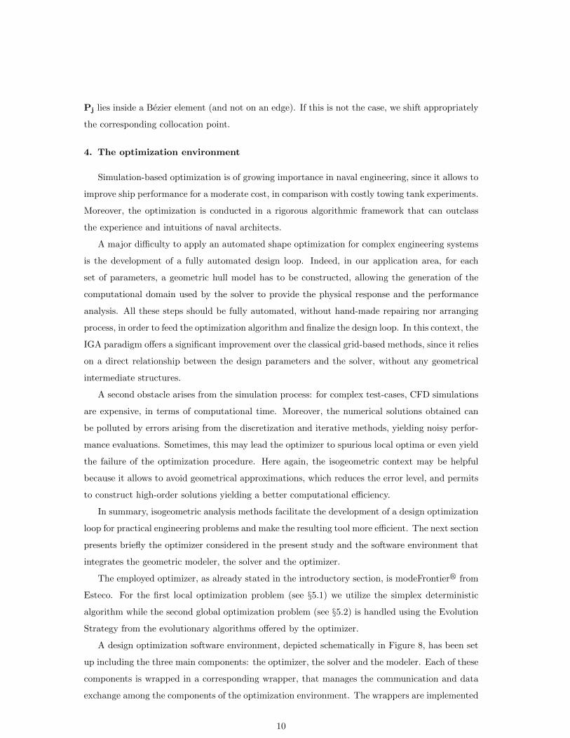
A design optimization software environment, depicted schematically in Figure 8, has been set

up including the three main components: the optimizer, the solver and the modeler. Each of these

components is wrapped in a corresponding wrapper, that manages the communication and data

exchange among the components of the optimization environment. The wrappers are implemented

10

using the python programming language and utilize the TCP/IP network protocol for the required

communications. More specifically:

1. Optimizer wrapper (Ow) communicates with the optimizer and broadcasts the generated

parameter values to the parametric modeler wrapper (Mw).

2. Mw listens for data connections from Ow. When data, i.e., parameter values, are received, it

triggers the Rhino construction script that produces the corresponding instance of the SPM

and ultimately stores it in an analysis suitable T-Spline file format (IGA file) at a specified

FTP site. If the creation of the IGA file is successful, Ow establishes a connection with

the Solver wrapper (Sw) and reports the IGA file creation. If the construction script fails a

message is returned to Ow reporting the failure and requesting a new parameter set.

3. When a new IGA file is received, Sw initiates a connection to the site where the IGA file

has been saved and retrieves it. IGA BEM solver is then started and performs the resistance

calculations resulting, if successful, in the broadcasting of the objective function(s) value(s)

to Ow. If computation fails, a network message is returned to Ow reporting the failure and

requesting a new parameter set.

As it is obvious from the above discussion Ow, Mw and Sw work at the same time as client

and server applications. This constitutes a flexible and efficient software environment for practical

tests, presented in the next section.

objective function value FTP address of T-spline representation (IGA format) of new hull model

DATA: new set of values for the design parameters & auxiliary control messages

OptimizerWrapper

outin out in inout

SolverWrapper Modeler

Wrapper

Figure 8: Schematic diagram of the optimization environment

5. Container-ship Optimization

The deployment platform for the optimization process is the following:

• The solver component runs in parallel and is deployed on a 8+1 linux cluster (1 head node

and 8 working nodes). Each working node is equipped with 2 Quadcore Intel Xeon 2.4GHz

CPUs with 12Gb Ram memory.

11

• Both the optimizer and the solver are deployed on a typical PC

• The intercommunications are carried out over Fast Ethernet connections.

The average time required for each step of the optimization loop is approximately 186 secs.

This is split among the processes as follows: On an average, 150 secs are spent in the solving

process and 25 secs are used by the modeler. The remaining part is spent by the optimizer and

intercommunications.

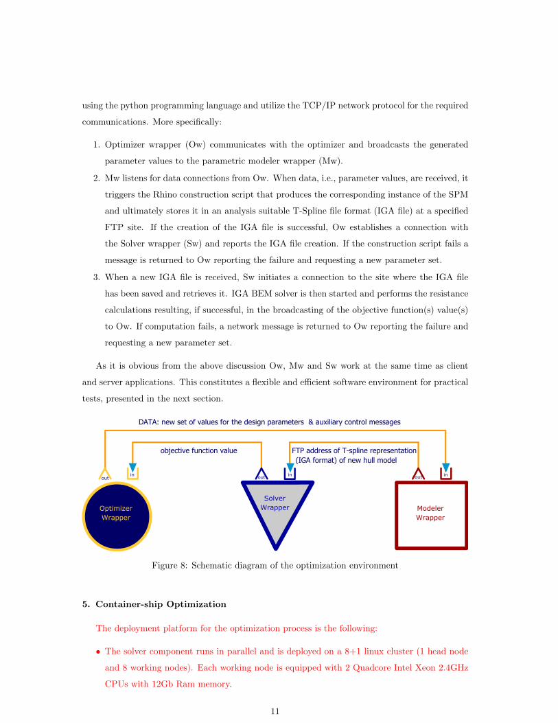
5.1. Constrained bow-optimization for minimizing wave resistance

The optimization environment has been firstly tested for optimizing the bow area of a container

ship against the criterion of minimum wave resistance, under the constraint of given displacement

V = 88581 m3. The main particulars of the ship have as follows: Lwl = 277 m, B = 32.2 m

T = 13.0 m, Cb = 0.734 and Vs=30 knots. Since we are interested in optimizing the bow ship

area, the design parameters are chosen to be: Bulb height, Bulb width, Bulb length, Fwd rise,

Bulb tip height with initial values (0.5, 0.7, 0.7, 0.2, 0.0), respectively ; see Fig. 9. The range of

variation of these parameters is given in the table depicted in Figure 9. The bound constraints are

handled by modeFrontier while the displacement constraint is fulfilled within the SPM construction

process.

Bulb_length

Bulb_tip_height

Fwd_rise

Bul

b_he

ight

Bulb_width

Parameters Min (ratio|value) Max (ratio|value)Bulb_height 0 | 0 m 1 | 2T/3Bulb_width 0 | 0 m 1 | B/5Bulb_length 0 | 0 m 1 | L/15Fwd_rise 0 | 0 m 1 | 2T/6Bulb_tip_height -1 | -T/3 1 | T/3

ConstraintsV = f(Bilge_R) = constant 88581 m3

Figure 9: Constrained bow optimization bulb parameters

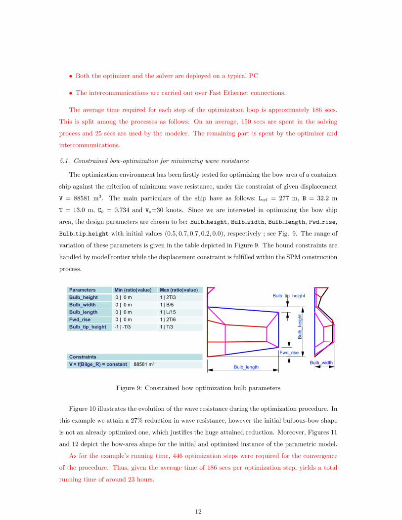
Figure 10 illustrates the evolution of the wave resistance during the optimization procedure. In

this example we attain a 27% reduction in wave resistance, however the initial bulbous-bow shape

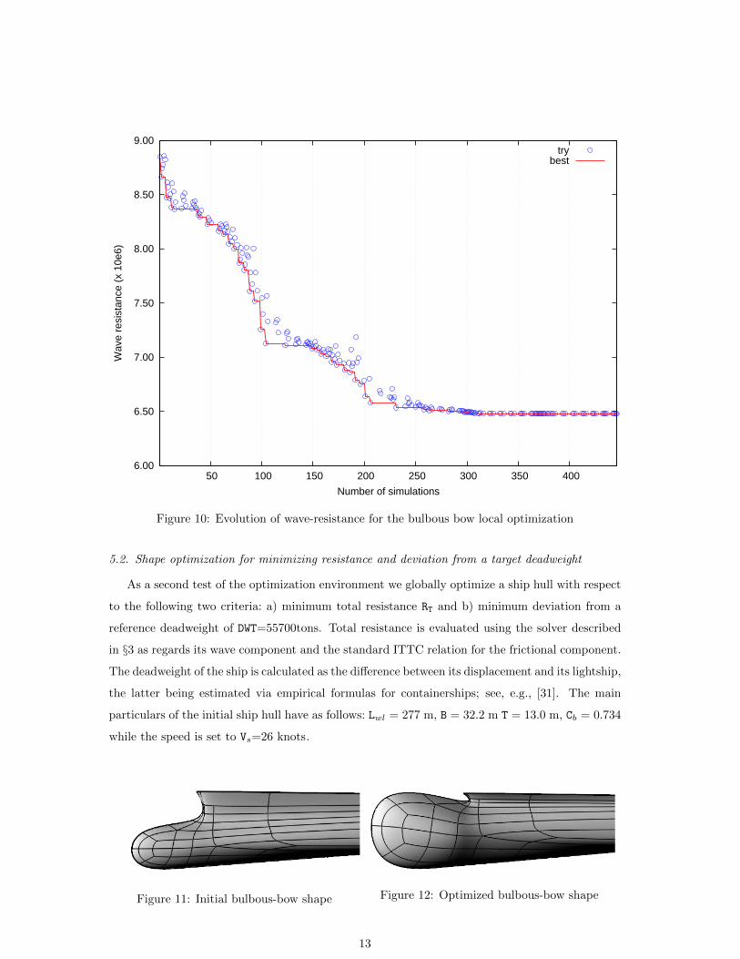
is not an already optimized one, which justifies the huge attained reduction. Moreover, Figures 11

and 12 depict the bow-area shape for the initial and optimized instance of the parametric model.

As for the example’s running time, 446 optimization steps were required for the convergence

of the procedure. Thus, given the average time of 186 secs per optimization step, yields a total

running time of around 23 hours.

12

6.00

6.50

7.00

7.50

8.00

8.50

9.00

50 100 150 200 250 300 350 400

Wav

e re

sist

ance

(x

10e6

)

Number of simulations

trybest

Figure 10: Evolution of wave-resistance for the bulbous bow local optimization

5.2. Shape optimization for minimizing resistance and deviation from a target deadweight

As a second test of the optimization environment we globally optimize a ship hull with respect

to the following two criteria: a) minimum total resistance RT and b) minimum deviation from a

reference deadweight of DWT=55700tons. Total resistance is evaluated using the solver described

in §3 as regards its wave component and the standard ITTC relation for the frictional component.

The deadweight of the ship is calculated as the difference between its displacement and its lightship,

the latter being estimated via empirical formulas for containerships; see, e.g., [31]. The main

particulars of the initial ship hull have as follows: Lwl = 277 m, B = 32.2 m T = 13.0 m, Cb = 0.734

while the speed is set to Vs=26 knots.

Figure 11: Initial bulbous-bow shape Figure 12: Optimized bulbous-bow shape

13

Seven design parameters are chosen for the optimization process, namely, the waterline length,

Lwl, the breadth, B, the longitudinal position of the parallel mid-body, Mid pos, the extent of the

parallel mid-body, Mid L, the bilge radius, Bilge R, the bulb length, Bulb length and the bulb

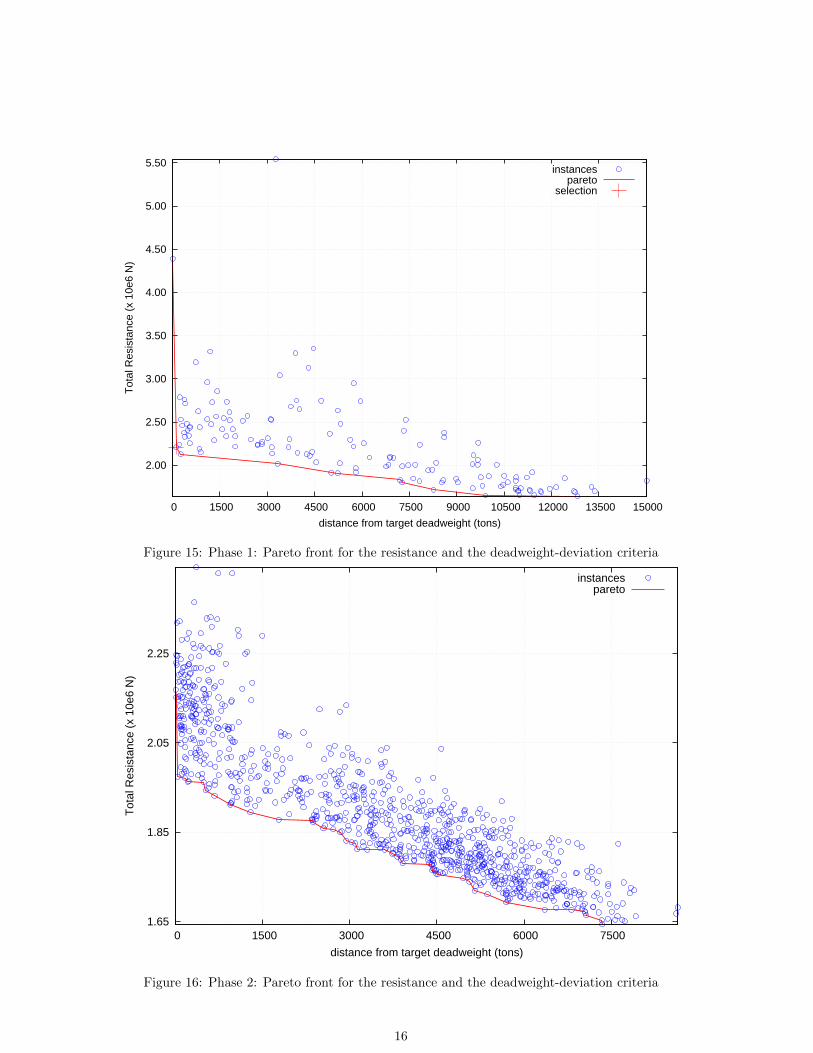
width, Bulb width; see Figures 1,2. The above parameters range as in Table 1. The evolution

strategy, offered by modeFrontier, is employed to calculate the Pareto front of the above optimiza-

tion problem, which is depicted in Figures 15,16, respectively. Figure 15 correspond to a first phase

of the optimization process where we try to coarsely cover the feasible space and select a suitable

candidate, as an initial point, for the second phase of the optimization process; see Figure 16. In

the first phase, the algorithm explores the feasible space with a large step size in order to catch

a coarse approximation of the Pareto front, while the second phase refines the step size starting

from the previously selected point at the Pareto front. Obviously, the optimum shapes lie on the

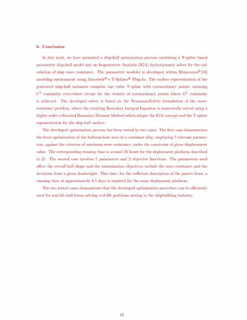
pareto front, red line depicted in Figure 16. If, for example, we choose to accept a 150tons devia-

tion from the target deadweight, the optimum solution would be the following ship-hull instance:

Lwl=295.5m, B=32.3m, Mid pos=0.458, Mid L=0.1245, Bilge R=0.0575, Bulb length=0.973 and

Bulb width=0.979 resulting in a resistance value of 1.915×106 and a deadweight deviation of 139

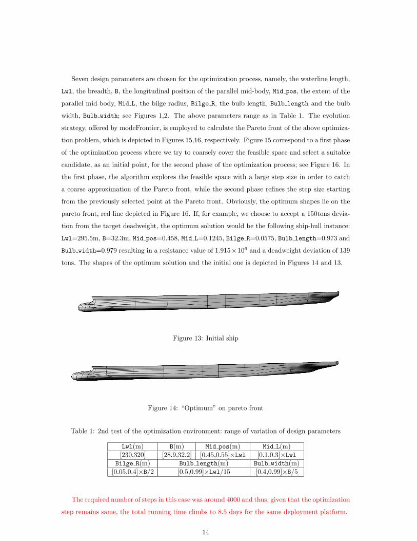
tons. The shapes of the optimum solution and the initial one is depicted in Figures 14 and 13.

Figure 13: Initial ship

Figure 14: “Optimum” on pareto front

Table 1: 2nd test of the optimization environment: range of variation of design parameters

Lwl(m) B(m) Mid pos(m) Mid L(m)[230,320] [28.9,32.2] [0.45,0.55]×Lwl [0.1,0.3]×Lwl

Bilge R(m) Bulb length(m) Bulb width(m)[0.05,0.4]×B/2 [0.5,0.99]×Lwl/15 [0.4,0.99]×B/5

The required number of steps in this case was around 4000 and thus, given that the optimization

step remains same, the total running time climbs to 8.5 days for the same deployment platform.

14

6. Conclusion

In this work, we have presented a ship-hull optimization process combining a T-spline based

parametric ship-hull model and an Isogeometric Analysis (IGA) hydrodynamic solver for the cal-

culation of ship wave resistance. The parametric modeler is developed within Rhinocerosr[10]

modeling environment using Autodeskr’s T-Splinesr Plug-In. The surface representation of the

generated ship-hull instances comprise one cubic T-spline with extraordinary points, ensuring

C2 continuity everywhere except for the vicinity of extraordinary points where G1 continuity

is achieved. The developed solver is based on the Neumann-Kelvin formulation of the wave-

resistance problem, where the resulting Boundary Integral Equation is numerically solved using a

higher order collocated Boundary Element Method which adopts the IGA concept and the T-spline

representation for the ship-hull surface.

The developed optimization process has been tested in two cases: The first case demonstrates

the local optimization of the bulbous-bow area of a container ship, employing 5 relevant parame-

ters, against the criterion of minimum wave resistance, under the constraint of given displacement

value. The corresponding running time is around 23 hours for the deployment platform described

in §5. The second case involves 7 parameters and 2 objective functions. The parameters used

affect the overall hull shape and the minimization objectives include the wave resistance and the

deviation from a given deadweight. This time, for the sufficient description of the pareto front, a

running time of approximately 8.5 days is required for the same deployment platform.

The two tested cases demonstrate that the developed optimization procedure can be efficiently

used for real-life hull-forms solving real-life problems arising in the shipbuilding industry.

15

2.00

2.50

3.00

3.50

4.00

4.50

5.00

5.50

0 1500 3000 4500 6000 7500 9000 10500 12000 13500 15000

Tot

al R

esis

tanc

e (x

10e

6 N

)

distance from target deadweight (tons)

instancespareto

selection

Figure 15: Phase 1: Pareto front for the resistance and the deadweight-deviation criteria

1.65

1.85

2.05

2.25

0 1500 3000 4500 6000 7500

Tot

al R

esis

tanc

e (x

10e

6 N

)

distance from target deadweight (tons)

instancespareto

Figure 16: Phase 2: Pareto front for the resistance and the deadweight-deviation criteria

16

Acknowledgments

This research has been co-financed by the European Union (European Social Fund - ESF) and

Greek national funds through the Operational Program “Education and Lifelong Learning” of the

National Strategic Reference Framework (NSRF) - Research Funding Program: THALIS-UOA

(MIS 375891).

References

[1] T. J. R. Hughes, J. A. Cottrell, Y. Bazilevs, Isogeometric analysis: CAD, finite elements,

NURBS, exact geometry and mesh refinement, Computer Methods in Applied Mechanics

and Engineering 194 (2005) 4135–4195.

[2] Y. Bazilevs, V. M. Calo, J. A. Cottrell, J. A. Evans, T. J. R. Hughes, S. Lipton, M. A.

Scott, T. W. Sederberg, Isogeometric analysis using T-splines, Computer Methods in Applied

Mechanics and Engineering 199 (5-8) (2010) 229–263.

[3] M. A. Scott, R. N. Simpson, J. A. Evans, S. Lipton, S. P. A. Bordas, T. J. R.

Hughes, T. Sederberg, Isogeometric boundary element analysis using unstructured T-splines,

Computer Methods in Applied Mechanics and Engineering 254 (0) (2013) 197 – 221.

doi:http://dx.doi.org/10.1016/j.cma.2012.11.001.

URL http://www.sciencedirect.com/science/article/pii/S0045782512003386

[4] T. W. Sederberg, J. Zheng, A. Bakenov, A. Nasri, T-splines and TNURCCs, ACM Transac-

tions on Graphics 22 (2003) 477–484.

[5] T. W. Sederberg, D. L. Cardon, G. T. Finnigan, N. S. North, J. Zheng, T. Lyche, T-spline

simplification and local refinement, ACM Transactions on Graphics 23 (2004) 276–283.

[6] A. P. Nagy, M. M. Abdalla, Z. Grdal, Isogeometric sizing and shape optimization of beam

structures, in: 50th AIAA/ASME/ASCE/AHS/ASC Structures, Structural Dynamics, and

Materials Conference, Palm Springs, California, USA, 2009.

[7] D. Nguyen, A. Evgrafov, J. Gravesen, Isogeometric shape optimization for electromagnetic

scattering problems, Progress In Electromagnetics Research 45 (2012) 117–146.

[8] P. Nørtoft, J. Gravesen, Isogeometric shape optimization in fluid mechanics, Structural and

Multidisciplinary Optimization 48 (2013) 909–925.

[9] H. Lian, R. Simpson, S. Bordas, Sensitivity analysis and shape optimisation through a t-spline

isogeometric boundary element method, in: International Conference on Computational Me-

chanics (CM13), Durham, UK, 2013.

17

[10] Robert McNeel & Associates, Rhinoceros, design, model, present, analyze, realize... (2014).

URL http://www.rhino3d.com/

[11] Autodesk Inc, T-splines for rhino (2014).

URL http://www.tsplines.com/

[12] H. Lackenby, On the Systematic Geometrical Variation of Ship Form, RINA-Transactions 92,

1950.

[13] S. Harries, H. Nowacki, Form Parameter Approach to the Design of Fair Hull Shapes, in:

10th International Conference on Computer Applications (ICCAS), MIT, Cambridge, MA,

USA, 1999.

[14] H. C. Kim, Parametric Design of Ship Hull Forms with a Complex Multiple Domain Surface

Topology, Ph.D. thesis, University of Berlin (2004).

[15] C. Abt, S. Harries, A New Approach to Integration of CAD and CFD for Naval Architects,

in: 6th International Conference on Computer Applications and Information Technology in

Maritime Industries (COMPIT), Cortona, Italy, 2007.

[16] S. Harries, Serious Play in Ship Design, in: Tradition and Future of Ship Design in Berlin.,

Technical University of Berlin, 2008.

[17] P. Zhang, D.-X. Zhu, Parametric Approach to Design of Hull Forms, Journal of Hydrody-

namics 20 (6) (2008) 804–810.

[18] A. I. Ginnis, C. Feurer, K. A. Belibassakis, P. D. Kaklis, K. V. Kostas, T. P. Gerostathis,

C. G. Politis, A catia R© ship-parametric model for isogeometric hull optimization with respect

to wave resistance, in: ICCAS 2011, Royal Institution of Naval Architects, 2011.

[19] A. I. Ginnis, R. Duvigneau, C. Politis, K. V. Kostas, K. Belibassakis, T. Gerostathis, P. D.

Kaklis, A Multi-Objective Optimization Environment for Ship-Hull Design based on a BEM-

Isogeometric Solver, in: The fifth Conference on Computational Methods in Marine Engi-

neering (Marine 2013), Hamburg, Germany, on 29-31 May 2013, springer, 2013.

[20] Dassault Systemes, Computer-Aided Three-Dimensional Interactive Application (2014).

URL http://www.3ds.com/products-services/catia/

[21] A. I. Ginnis, K. V. Kostas, C. G. Politis, P. D. Kaklis, K. A. Belibassakis, T. P. Gerostathis,

M. A. Scott, T. J. R. Hughes, Isogeometric Boundary-Element Analysis for the Wave-

Resistance Problem using T-splines, Computer Methods in Applied Mechanics and Engi-

neering, submitted 2014.

18

[22] R. Sharma, T.-W. Kim, R. Lee Storch, H. J. Hopman, S. O. Erikstad, Challenges in computer

applications for ship and floating structure design and analysis, CAD 44 (2012) 166–185.

[23] H. J. Koelman, A Mid-Term Outlook on Computer Aided Ship Design, in: COMPIT’13

Proceedings of the 12th International Conference on Computer Applications and Information

Technology in the Maritime Industries, Ancona, Italy, 2013, pp. 110–119.

[24] R. Brard, The representation of a given ship form by singularity distributions when the

boundary condition on the free surface is linearized, Ship Research 16 (1972) 79–82.

[25] J. J. M. Baar, W. G. Price, Developments in the Calculation of the Wavemaking Resis-

tance of Ships, Proc. Royal Society of London. Series A, Mathematical and Physical Sciences

462 (1850) (1988) 115–147.

[26] M. Scott, T. Hughes, T. Sederberg, M. Sederberg, An integrated approach to engineering

design and analysis using the autodesk t-spline plugin for rhino3d, Advances in Engineering

Software (in preparation).

[27] Esteco, Integration platform for multi-objective and multi-disciplinary optimization (2014).

URL http://www.esteco.com/modefrontier

[28] J. A. Cottrell, T. J. R. Hughes, A. Reali, Studies of refinement and continuity in isogeometric

structural analysis, Computer Methods in Applied Mechanics and Engineering 196 (2007)

4160–4183.

[29] J. A. Cottrell, T. J. R. Hughes, Y. Bazilevs, Isogeometric Analysis: Toward Integration of

CAD and FEA, Wiley, 2009.

[30] K. A. Belibassakis, T. P. Gerosthathis, K. V. Kostas, C. G. Politis, P. D. Kaklis, A.-A.

Ginnis, C. Feurer, A BEM-Isogeometric method for the ship wave-resistance problem, Ocean

Engineering 60 (2013) 53–67.

[31] Y. Chen, Formulation of a Multi-Disciplinary Design Optimization of Containerships, Mas-

ter’s thesis, Virginia Polytechnic Institute and State University, USA (1999).

19