SHIP target cooling flow simulations

SHIP – target cooling flow simulations

Preliminary results

18/18/2015 1A. Rakai, P. Pachołek

P. Pachołek 28/18/2015

General apporach to heat transfer coefficient calculations

Approach: gap-wise, minimize the standard deviation of temperature drop (along the length) – this would

imply that heat transfer conditions are the same in all channels.

In general, to calculate the temperature drop in the channel one can use the following equation

and solve for Ts. However, the heat transfer coeffcient (HTC), h, bulk fluid temperature, T∞ and dissipated

power, Q, have to be explicitly know. As Q and T∞ can be considered given for our problem, only HTC

has to be calculated. HTC is in general a function of dimensionless Nusselt number.

Nu numberr in turn depends on Reynolds and Prandtl numbers. The empirical correlation used for

calculation of Nu number for flows in ducts was given by Dittus and Boelter and is as follows:

where

A. Rakai, P. Pachołek 38/18/2015

Summary

Based on the simulations done for heat load of 1 pulse uniformly distrubuted in 7.2

seconds, the following conclusions can be drawn:

• while theoretically a flow of 4 litres/second is theoretically capable of removing the heat

from the system with a water temperature increase of 20 ºC, uneven flow distribution

across the gaps, as well as boundary layer effects will cause the water to heat up locally

by over 300 ºC

• The local heat-up effect is less pronounced for a flow of 16 l/s - the maximum local

temperature in the channels is between 100 and 140 ºC (depending on the manifold

setup) and occurs in the middle of the gaps, where water is exposed to highest wall

temperatures.

• For a flow of 16 l/s average water temperature in each of the gaps is ca. 25 ºC

• Maximum local and average wall temperatures follow the results for water

• For a flow of 16 l/s a pressure drop between 50 (constant manifold cross-section area)

to 75 mbar (sloped manifolds) is expected in the system

• All three tested turbulence models (standard k-epsilon, realizable k-epsilon, transition

SST) provide similar results\

• A transient simulation accounting for heat load being


Analytical approach - continued

Altogether, this shows that the heat transfer coefficient is a function of hydraulic diameter (thus: the gap

size as well).

The problem is that is an increasing function (as shown in the picture below), thus when the gap

size increases, the heat transfer coefficient goes down and the surface temperature increases. Therefore

for the stated optimization problem, in spots where heat load is the highest, the gap size would be

chosen as small as possible, while in spots where heat load is the lowest, the „ideal” gap size would be

as high as possible.

Function y=f(x0.2)


Analytical results

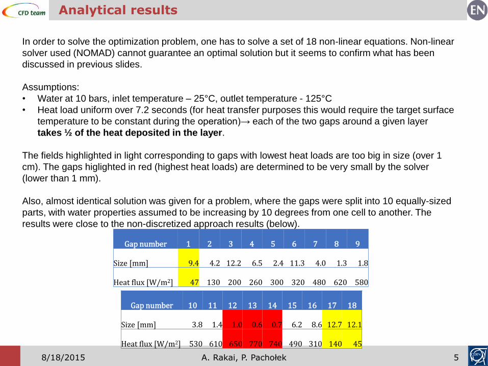
Gap number 1 2 3 4 5 6 7 8 9

Size [mm] 9.4 4.2 12.2 6.5 2.4 11.3 4.0 1.3 1.8

Heat flux [W/m2] 47 130 200 260 300 320 480 620 580

Gap number 10 11 12 13 14 15 16 17 18

Size [mm] 3.8 1.4 1.0 0.6 0.7 6.2 8.6 12.7 12.1

Heat flux [W/m2] 530 610 650 770 740 490 310 140 45

In order to solve the optimization problem, one has to solve a set of 18 non-linear equations. Non-linear

solver used (NOMAD) cannot guarantee an optimal solution but it seems to confirm what has been

discussed in previous slides.

Assumptions:

• Water at 10 bars, inlet temperature – 25°C, outlet temperature - 125°C

• Heat load uniform over 7.2 seconds (for heat transfer purposes this would require the target surface

temperature to be constant during the operation)→ each of the two gaps around a given layer

takes ½ of the heat deposited in the layer.

The fields highlighted in light corresponding to gaps with lowest heat loads are too big in size (over 1

cm). The gaps higlighted in red (highest heat loads) are determined to be very small by the solver

(lower than 1 mm).

Also, almost identical solution was given for a problem, where the gaps were split into 10 equally-sized

parts, with water properties assumed to be increasing by 10 degrees from one cell to another. The

results were close to the non-discretized approach results (below).


Preliminary CFD results

Under the same assumptions as in analytical considerations, CFD studies have shown, that for the gap

with the critical heat load (corresponding to layer 13) a width of 0.5 cm assuming a 0.35 m/s velocity

should be sufficient – maximum temperature of water in the gap would then be 90 °C (outlet).

This is also true for the gaps with the critical volumetric heat load (gaps 6 and 7) – in that case the

maximum temperature of water in the gap (for a width of 0.5 cm and flow velocity of 0.35 m/s) was

calculated to be 70 °C (also at the outlet).


Summary

Based on the simulations done for heat load of 1 pulse uniformly distrubuted in 7.2

seconds, the following conclusions can be drawn:

• while a flow of 4 litres/second is theoretically capable of removing the heat from the

system with a water temperature increase of 20 ºC, uneven flow distribution across the

gaps, as well as boundary layer effects will cause the water to heat up locally by over

300 ºC

• The local heat-up effect is less pronounced for a flow of 16 l/s - the maximum local

temperature in the channels is between 100 and 140 ºC and occurs in the middle of the

gaps, where water is exposed to highest wall temperatures. This corresponds to a HTC

of 10000 – 20000 W/m2K

• For a flow of 16 l/s average water temperature in each of the gaps is ca. 27 ºC

• Obviously, maximum local and average wall temperatures follow the results for water

• For a flow of 16 l/s a pressure drop between 50 (constant manifold cross-section area)

to 75 mbar (sloped manifolds) is expected in the system

• All three tested turbulence models (standard k-epsilon, realizable k-epsilon, transition

SST) provide similar results

• A transient simulation accounting for heat load being non-uniform over 7.2

seconds needs to be investigated in order to understand its influence on the local

conditions in the boundary layer


Velocity distribution – sloped and non-sloped manifolds

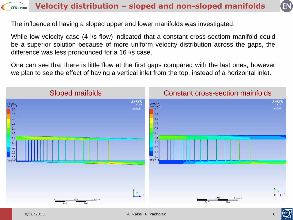
The influence of having a sloped upper and lower manifolds was investigated.

While low velocity case (4 l/s flow) indicated that a constant cross-sectiom manifold could

be a superior solution because of more uniform velocity distribution across the gaps, the

difference was less pronounced for a 16 l/s case.

One can see that there is little flow at the first gaps compared with the last ones, however

we plan to see the effect of having a vertical inlet from the top, instead of a horizontal inlet.

Sloped maifolds Constant cross-section mainfolds


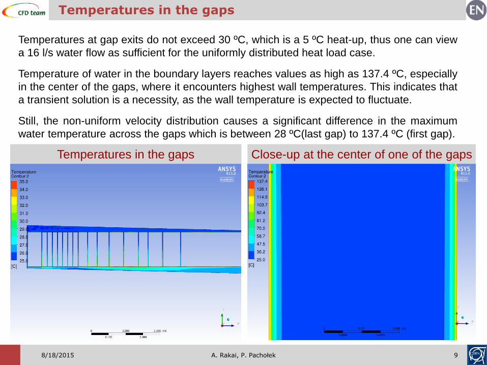
Temperatures in the gaps

Temperatures at gap exits do not exceed 30 ºC, which is a 5 ºC heat-up, thus one can view

a 16 l/s water flow as sufficient for the uniformly distributed heat load case.

Temperature of water in the boundary layers reaches values as high as 137.4 ºC, especially

in the center of the gaps, where it encounters highest wall temperatures. This indicates that

a transient solution is a necessity, as the wall temperature is expected to fluctuate.

Still, the non-uniform velocity distribution causes a significant difference in the maximum

water temperature across the gaps which is between 28 ºC(last gap) to 137.4 ºC (first gap).

Temperatures in the gaps Close-up at the center of one of the gaps


Heat transfer coefficient and maximum block temperature

The heat transfer coefficient in the 16 l/s case varies between around 10000 W/m2K

encountered in the first gaps, where the velocity is the lowest, up to 20000-25000 W/m2K in

the last gaps with the highest flow velocity.

Under the assumption of uniform heat load over pulse period, the maximum block

temperature of 282 ºC is observed in block 13.

Heat transfer coefficient Close-up at the center of one of the gaps


To be investigated

• numerical sensitivity, mesh dependence

• E deposition based gap distribution

• evening velocity distribution in gaps

• transient simulation


Summary

Several simulations, both transient and steady-state, were conducted in order to find an

appropriate solution for cooling of the SHIP target. The conclusions are as follows:

• A system of 4 inlet and 4 outlet pipes, all of 9 cm diameter, seems to be able to make

the velocity distribution in the gaps uniform.

• The widths of the gaps are not as crucial to the problem as the distribution of the flow.

Bulk fluid temperature remains low for any velocity close to 2 m/s. Gaps thinner than 0.5

cm could also be capable of removing the heat, however the pressure drop will surely

affect the velocity distribution in such case.

• With lower flow velocities it is possible to evacuate the heat as well, however boundary

layer effects will cause the water to heat up significantly close to the walls and this

needs to be tackled by using velocities higher than the analytically derived ones.

• For transient simulations, quasi-steady state of the system is reached after 5 pulses.

There is only a slight difference in temperature of water after the 3rd pulse.

• In the transient simulation - the maximum local temperature in the channels stands at

120 ºC, corresponding to heat transfer coefficients of ca. 20000 W/m2K.

• For a flow of 50 l/s a pressure drop of ca. 160 mbar is expected in the system

• Mesh independence study needs to be done for transient simulation due to

varying heat transfer conditions. Also, temperatures in the gaps could be

equalized by assuming a linear relation between heat deposition and gap width.


Velocity distribution – qualitative results

After several tested arrangements of the inlet and outlet pipes, 2 transient cases were ran,

for flows of 50 and 80 l/s. The arrangement allowed for a singificantly more uniform

distribution of velocities in the gaps, thus reducing the maximum recorded temperature.

Note that for simplifcation the inlet and outlets are simulated as squares with sides of 8 cm

which corresponds to an area of a pipe of 9 cm inner diameter.

Pictures below show the velocity at the mid-X plane cross-section (vertical cut) for transient

simulation after 1 pulse. The velocity scale differs for each of the pictures.

Velocity after 1 pulse – 50 l/s flow Velocity after 1 pulse – 80 l/s flow


Velocity distribution– quantitative results

The plot below presents the velocity distribution in the gaps. One can immediately see that

the graphs follow the same trend, indicating that the conditions change linearly with

increase of the flow rate, i.e. if inlet velocity is changed by a factor of 2, it is expected the

velocity in the gaps increases by a factor of 2 as well.

For a system of equally sized gaps it is important to have high flow in spots where more

heat is deposited, which in our case are, in general, the blocks which are 2.5 cm wide.

Although block 1 is exposed to the smallest flow, it contains higher heat capacity than the

thinner blocks and the flow observed was sufficient to keep it reasonably cooled.

0

0.5

1

1.5

2

2.5

3

3.5

4

4.5

5

0 1 2 3 4 5 6 7 8 9 10 11 12 13 14 15 16 17

Average velocity in the gaps [m/s]

50 l/s 80 l/s


Temperatures in the gaps

For both flows of 50 and 80 l/s, the temperatures at gap exits are in the range of 0-3 ºC,

showing that both of these flows are sufficient to keep the system cooled.

Temperature of the coolant in the boundary layers reaches values up to 120 ºC, still below

the evaporation temperature for water at 10 bar standing at 180 ºC.

Even though the flow has been significantly uniformized compared to the previously

presented results, due to different heat deposition in the blocks, the maximum registered

temperature varies between 3 to 100 ºC after 1 pulse. Local maximum temperatures were

registered for the blocks, which are located in between the inlet pipes, due to the two flows

having opposite directions collide and in result the velocity is lower.

0

20

40

60

80

100

120

0 1 2 3 4 5 6 7 8 9 10 11 12 13 14 15 16 17

Maximum temperature [°C] in the gaps after 1 pulse

50 l/s 80 l/s


Heat transfer coefficient and maximum block temperatures

The heat transfer coefficient in the 50 l/s case varies between around 15000-20000 W/m2K,

with the average being 19000 W/m2K, while for flow of 80 l/s it is slightly higher at 21000

W/m2K.

For the two flows, different blocks are predicted as the ones with highest temperature – in

case of the lower flow, it is block 6 at 303 ºC, while for the higher – block 9 at 266 ºC.

Another simulation with heat deposition averaged over 7.2 seconds and 50 l/s flow showed

that the maximum temperature is 271 ºC in block 9.

Block temperature – 50 l/s flow Block temperature – 80 l/s flow


Thank you for your attention!

Documents

SHIP target cooling flow simulations