Embed Size (px)
Citation preview
SHOCK FAILURE ANALYSIS OF MILITARY EQUIPMENTS BY USING STRAIN ENERGY DENSITY
A THESIS SUBMITTED TO THE GRADUATE SCHOOL OF NATURAL AND APPLIED SCIENCES
OF MIDDLE EAST TECHNICAL UNIVERSITY
BY
ÜMĐT MERCĐMEK
IN PARTIAL FULFILLMENT OF THE REQUIREMENTS
FOR THE DEGREE OF MASTER OF SCIENCE
IN MECHANICAL ENGINEERING
DECEMBER 2010
Approval of the thesis:
SHOCK FAILURE ANALYSIS OF MILITARY EQUIPMENTS BY USING STRAIN ENERGY DENSITY
submitted by ÜMĐT MERC ĐMEK in partial fulfillment of the requirements for the degree of Master of Science in Mechanical Engineering Department, Middle East Technical University by, Prof. Dr. Canan Özgen Dean, Graduate School of Natural and Applied Sciences Prof. Dr. Süha Oral Head of Department, Mechanical Engineering Prof. Dr. F. Suat Kadıoğlu Supervisor, Mechanical Engineering Dept., METU Prof. Dr. Mehmet Çelik Co. Supervisor, Mechatronic Eng. Dept., KTO Karatay University Examining Committee Members: Prof. Dr. Y. Samim Ünlüsoy Mechanical Engineering Dept., METU Prof. Dr. F. Suat Kadıoğlu Mechanical Engineering Dept., METU Prof. Dr. Metin Akkök Mechanical Engineering Dept., METU Prof. Dr. Mehmet Çelik Mechatronic Engineering Dept., KTO Karatay University Asst. Prof. Dr. Yiğit Yazıcıoğlu Mechanical Engineering Dept., METU
Date: 07/12/2010

iii
I hereby declare that all information in this document has been obtained and presented in accordance with academic rules and ethical conduct. I also declare that, as required by these rules and conduct, I have fully cited and referenced all material and results that are not original to this work.
Name, Last Name: Ümit MERCĐMEK
Signature:
iv
ABSTRACT
SHOCK FAILURE ANALYSIS OF MILITARY EQUIPMENTS BY USING STRAIN ENERGY DENSITY
Mercimek, Ümit
M.S., Department of Mechanical Engineering
Supervisor: Prof. Dr. F. Suat Kadıoğlu
Co-Supervisor: Prof. Dr. Mehmet Çelik
December 2010, 123 pages
Failure of metallic structures operating under shock loading is a common
occurrence in engineering applications. It is difficult to estimate the response of
complicated systems analytically, due to structure’s dynamic characteristics and
varying loadings. Therefore, experimental, numerical or a combination of both
methods are used for evaluations.
The experimental analysis of the shocks due to firing is done for 12.7mm
Gatling gun and 25mm cannon. During the tests, the Gatling gun and the cannon
are located on military Stabilized Machine Gun Platform and Stabilized Cannon
Platform respectively.
For the firing tests, ICP (integrated circuit piezoelectric) accelerometers are
attached to obtain the loading history for corresponding points. Shock Response
Spectrum (SRS) analysis (nCode Glypworks) is done to define the equivalent
shock profiles created on test pieces and the mount of 25mm cannon by means
v
of the gun and the cannon firing. Transient shock analysis of the test pieces and
the mount are done by applying the obtained shock profiles on the parts in a
finite element model (ANSYS).
Furthermore, experimental stress analysis due to shock loading is performed for
two different types of material and different thicknesses of the test pieces. The
input data for the analysis is obtained through measurements from strain rosette
precisely located at the critical location of the test pieces.
As a result of the thesis, a proposal is tried to be introduced where strain energy
density theory is applied to predict the shock failure at military structures.
Keywords: Shock Failure, SRS, Strain Energy Density, Experimental Stress
Analysis, Finite Elements Analysis.
vi
ÖZ
ASKERĐ MALZEMELERDE GER ĐNĐM ENERJĐSĐ YOĞUNLUĞUNU KULLANARAK ŞOK KIRILMA ANAL ĐZĐ
Mercimek, Ümit
Yüksek Lisans, Makine Mühendisliği Bölümü
Tez Yöneticisi: Prof. Dr. F. Suat Kadıoğlu
Ortak Tez Yöneticisi: Prof. Dr. Mehmet Çelik
Aralık 2010, 123 sayfa
Mühendislik uygulamalarında, şok yükü altında çalışan yapılarda sıklıkla metal
hasarları görülmektedir. Yapıların dinamik özellikleri ve değişken yüklerden
dolayı sistemlerin tepkilerini analitik olarak tespit etmek zor olmaktadır. Bu
nedenle, hesaplamalar için deneysel yöntemler, sayısal metotlar veya her iki
yöntem birlikte kullanılmaktadır.
Bu tezde, 12.7mm Gatling silahı ve 25mm top atışları kaynaklı oluşan şokların
deneysel analizi gerçekleştirilmi ştir. Testler esnasında Gatling silahı Stabilize
Makineli Tüfek Platformu (STAMP), top ise Stabilize Top Platformu (STOP)
üzerine yerleştirilmi ştir.
Atış testlerinde, belirlenen noktalardaki şok yüklemesini elde edebilmek için
ICP (integrated circuit piezoelectric) ivmeölçerler yerleştirilmi ştir. Silah ve top
atışları sırasında test parçaları ve top bağlantı parçası üzerinde oluşan şok
yüklerine eşdeğer şok profillerini tanımlayabilmek için Şok Tepki Spektrum
vii
(STS) analizleri (nCode Glypworks) yapılmıştır. Elde edilen şok profilleri ve
sayısal analiz modeli (ANSYS) kullanılarak test parçaları ve top bağlantı
parçası için zamana bağlı şok analizleri gerçekleştirilmi ştir.
Ayrıca, şok yüklemesi için, iki farklı test parçası malzemesi ve farklı
kalınlıklardaki test parçaları kullanılarak deneysel gerilme analizleri yapılmıştır.
Bu analizlerde kullanılan girdiler test parçalarının kritik bölgelerine hassas bir
şekilde yerleştirilen gerinim ölçerlerden alınan ölçüm sonuçlarıdır.
Tezde sonuç olarak, askeri yapılarda şok kırılmasına karar verebilmek için
gerinim enerji yoğunluğu teorisinin uygun olduğu değerlendirmesi ortaya
koyulmaya çalışılmıştır.
Anahtar Kelimeler: Şok Yorulması, STS, Gerinim Enerjisi Yoğunluğu,
Deneysel Gerilme Analizi, Sonlu Elemanlar Analizi.

viii
To My Family

ix
ACKNOWLEDGEMENTS
I am grateful to my thesis supervisor Prof. Dr. Suat KADIOĞLU and co-
supervisor Prof. Dr. Mehmet ÇELĐK for their guidance, support and helpful
criticism throughout the progress of my thesis study.
I would like to thank my friend Fatih ALTUNEL for his help.
The cooperation and friendly support of my colleagues in ASELSAN during my
thesis study also deserves to be acknowledged.
Thanks to my parents, brother and sister for their unique motivation and
encouragement.
Finally, many thanks to my wife Esin MERCĐMEK for her continuous help and
understanding during my thesis study.
x
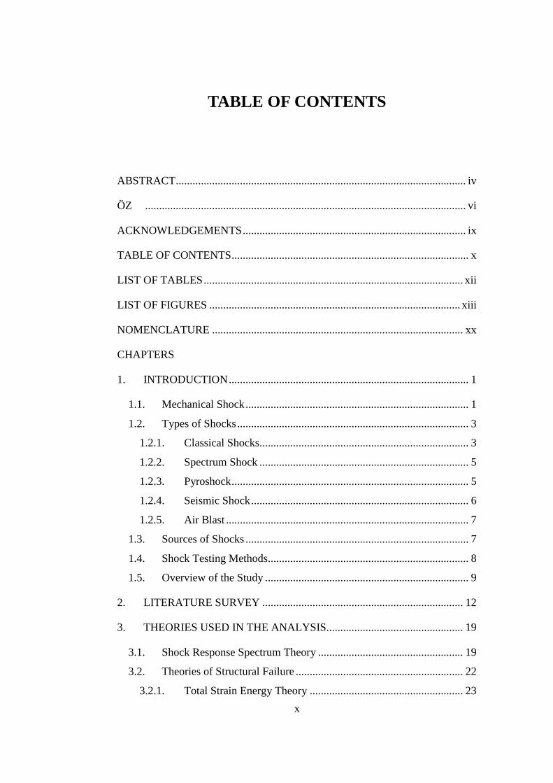
TABLE OF CONTENTS
ABSTRACT ........................................................................................................ iv
ÖZ ................................................................................................................... vi
ACKNOWLEDGEMENTS ................................................................................ ix
TABLE OF CONTENTS ..................................................................................... x
LIST OF TABLES ............................................................................................. xii
LIST OF FIGURES .......................................................................................... xiii
NOMENCLATURE .......................................................................................... xx
CHAPTERS
1. INTRODUCTION ...................................................................................... 1
1.1. Mechanical Shock ................................................................................ 1
1.2. Types of Shocks ................................................................................... 3
1.2.1. Classical Shocks........................................................................... 3
1.2.2. Spectrum Shock ........................................................................... 5
1.2.3. Pyroshock ..................................................................................... 5
1.2.4. Seismic Shock .............................................................................. 6
1.2.5. Air Blast ....................................................................................... 7
1.3. Sources of Shocks ................................................................................ 7
1.4. Shock Testing Methods........................................................................ 8
1.5. Overview of the Study ......................................................................... 9
2. LITERATURE SURVEY ........................................................................ 12
3. THEORIES USED IN THE ANALYSIS................................................. 19
3.1. Shock Response Spectrum Theory .................................................... 19
3.2. Theories of Structural Failure ............................................................ 22
3.2.1. Total Strain Energy Theory ....................................................... 23
xi
3.2.2. Distortion Energy Theory .......................................................... 25
3.2.3. Plastic Deformation ................................................................... 25
3.3 Transient Response Analysis ......................................................... 29
3.3.1. Newmark’s Method ................................................................... 30
4. FIRING TESTS AND DATA ACQUISITION ....................................... 32
5. NUMERICAL AND EXPERIMENTAL SHOCK ANALYSIS .............. 39
5.1. Shock Response Spectrum Analysis .................................................. 39
5.2. Experimental Stress Analysis ............................................................ 44
5.3. Numerical (FEM) Analysis of Test Pieces ........................................ 48
5.4. Evaluations of the Results .................................................................. 58
5.5. Application of the Theory to a System in Use ................................... 64
6. DISCUSSION AND CONCLUSIONS .................................................... 72
REFERENCES .................................................................................................. 76
APPENDICES
A. EQUIPMENT USED THROUGHOUT TESTS ...................................... 80
B. STRAIN ROSETTE ANALYSIS ............................................................ 83
B.1 Rectangular Rosette ........................................................................... 84
B.2 Principal Stresses ............................................................................... 85
C. TENSILE TEST OF THE CAST ALUMINUM ...................................... 86
D. EXPERIMENTAL RESULTS OBTAINED BY USING ESAM ............ 88
E. NUMERICAL (ANSYS TRANSIENT) ANALYSIS RESULTS
OBTAINED BY USING ANSYS ............................................................ 94
F. SAMPLE ANALYSIS OF STRAIN ENERGY DENSITY IN ANSYS .....
................................................................................................................ 119
xii
LIST OF TABLES
TABLES
Table 4.1 Visual Inspection Results of Rosette Analysis Tests ........................ 38
Table 5.1 Maximum and Minimum Principal Stresses Results of Rosette
Analysis Tests.................................................................................... 46
Table 5.2 Material Properties of 7075-T7351 Aluminum ................................ 49
Table 5.3 Structural Material Properties for 7075-T7351 Al in ANSYS .......... 51
Table 5.4 Bilinear Isotropic Hardening Properties for 7075-T7351 Al in ANSYS
........................................................................................................... 51
Table 5.5 Results of ANSYS on the Cast Aluminum Test Pieces .................... 57
Table 5.6 Results of ANSYS on the 7075 Aluminum Test Pieces ................... 58
Table 5.7 Material Properties of Impax Steel ................................................... 65
Table 5.8 Material Properties for Impax Steel in ANSYS ................................ 66
Table 5.9 Bilinear Isotropic Hardening Properties for Impax Steel in ANSYS ...
........................................................................................................ 66
Table 5.10 Results of ANSYS Transient Response on the 25mm Cannon Mount
........................................................................................................... 71
Table C.1 Tensile Tests Inputs and Outputs for Cast Aluminum ..................... 86
Table F.1 Strain Energy Density Results of ANSYS for the Sample Bar ...... 123
xiii
LIST OF FIGURES
FIGURES
Figure 1.1 Various Shock Input Pulses ................................................................ 1
Figure 1.2 Response of System to Rectangular Pulses of Varying Duration ...... 2
Figure 1.3 Examples of Mechanical Shock ......................................................... 3
Figure 1.4 Half-Sine (Haversine) ......................................................................... 4
Figure 1.5 Sawtooth Shock .................................................................................. 4
Figure 1.6 Triangle Shock.................................................................................... 5
Figure 1.7 Shock Spectrum .................................................................................. 5
Figure 1.8 Pyroshock Shock Response Spectrum................................................ 6
Figure 1.9 Seismic Shock Time History .............................................................. 6
Figure 1.10 Air blast ............................................................................................ 7
Figure 1.11 Application of a Test Piece on Gatling Gun ..................................... 9
Figure 1.12 A Test Piece used for Experimental Analysis ................................ 10
Figure 1.13 Application of a Mount on 25mm Cannon ..................................... 10
Figure 3.1 Shock Response Spectrum Model .................................................... 20
Figure 3.2 Free-body Diagram of SDOF System .............................................. 20
Figure 3.3 Sample of a Shock Response Spectrum ........................................... 22
Figure 3.4 Strain Energy Density by using Stress-Strain Curve ........................ 24
Figure 3.5 Strain Energy Density - Different Types of Materials ..................... 24
Figure 3.6 Stress and Strain Relation ................................................................. 26
Figure 3.7 Isotropic (left) and kinematic (right) hardening Circle represents the
yield surface ...................................................................................... 28
Figure 4.1 A View of Stabilized GAU19/A 12.7mm Gatling Gun System ...... 32
Figure 4.2 A View of Stabilized KBA 25mm Cannon System ......................... 32
Figure 4.3 ICP accelerometers ........................................................................... 33
Figure 4.4 Locations of the Test Parts and the Accelerometers on them .......... 33
Figure 4.5 Acceleration “g” vs Time “sec” Signal ............................................ 34
Figure 4.6 A Test Piece Equipped with a Strain Rosettes ................................. 35
xiv
Figure 4.7 Rosettes Inputs, Calibration and Balancing Screen .......................... 35
Figure 4.8 Rosette Calibration Screen ............................................................... 36
Figure 4.9 Different Material or Thicknesses of Test Pieces............................. 36
Figure 4.10 A Raw strain data for a gage part of the analyzed rosette .............. 37
Figure 4.11 Cast Aluminum Test Pieces Examples After The Tests ................. 37
Figure 4.12 7075-T7351 Aluminum Test Pieces Examples After The Tests .... 38
Figure 5.1 SRS Block Diagram ......................................................................... 40
Figure 5.2 SRS Graph Property – Time increases ............................................. 41
Figure 5.3 SRS Graph Property – Amplitude increases .................................... 41
Figure 5.4 SRS Graph Property – Classical shock form changes ...................... 42
Figure 5.5 ACC-TDC on Gatling Gun – Test4 (2mm CA Part Test) ................ 43
Figure 5.6 SRS Graph – Gatling Gun Test4 ...................................................... 43
Figure 5.7 Rosette Analysis Input Screen .......................................................... 44
Figure 5.8 Minimum Principal Stresses – SG Measurement (1mm CA) .......... 45
Figure 5.9 Maximum Principal Stresses – SG Measurement (1mm CA) .......... 46
Figure 5.10 Counting Result of Firing Test (3mm 7075 AL) ............................ 47
Figure 5.11 Mean Stress and AES (1mm 7075 AL) .......................................... 48
Figure 5.12 Mesh Model of the Test Piece ........................................................ 49
Figure 5.13 Bilinear Isotropic Hardening Graph for 7075-T7351 Al in ANSYS
......................................................................................................... 51
Figure 5.14 Thickness Definition of the Test Piece ........................................... 52
Figure 5.15 Shell Model of the Test Piece ......................................................... 52
Figure 5.16 Maximum Strain Energy for 300g 1ms ACC (1mm CA) .............. 53
Figure 5.17 Stress-Strain diagram for 7075-T7351 Aluminum ......................... 54
Figure 5.18 SMP Velocity Graph for 300g 1ms ACC (1mm Cast Aluminum) 55
Figure 5.19 SMP Maximum Principal Stresses for 300g 1ms ACC (1mm Cast
Aluminum) ...................................................................................... 55
Figure 5.20 SMP Minimum Principal Stresses for 300g 1ms ACC (1mm Cast
Aluminum) ...................................................................................... 56
Figure 5.21 SMP Equivalent Stresses Graph for 300g 1ms ACC (1mm Cast
Aluminum) ...................................................................................... 56
xv
Figure 5.22 Effect of Material Thickness on Maximum SED (Cast Aluminum)
......................................................................................................... 59
Figure 5.23 Effect of Material Thickness on Maximum SED (7075 Al) .......... 59
Figure 5.24 Effect of Material Thickness on SF of UTS (Cast Aluminum) ...... 60
Figure 5.25 Effect of Material Thickness on SF of UTS (7075 Al) .................. 61
Figure 5.26 Effect of Material Thickness on SF of SE (Cast Aluminum) ......... 62
Figure 5.27 Effect of Material Thickness on SF of SE (7075 Al) ..................... 62
Figure 5.28 Effect of Material Volume on Maximum SED (Cast Aluminum) . 63
Figure 5.29 Effect of Material Volume on Maximum SED (7075 Al) .............. 64
Figure 5.30 Mesh Model of the Mount .............................................................. 65
Figure 5.31 Bilinear Isotropic Hardening Graph for Impax Steel in ANSYS ... 66
Figure 5.32 ANSYS Model of the Mount .......................................................... 67
Figure 5.33 ACC-TDC on the Mount of 25mm Cannon – Test6 ...................... 68
Figure 5.34 SRS Graph – 25mm Cannon Test6 ................................................ 68
Figure 5.35 Maximum Strain Energy for 100g 2ms ACC (Impax Steel) .......... 69
Figure 5.36 Stress-Strain graph for Impax Steel ................................................ 70
Figure 5.37 SMP Velocity Graph for 100g 2ms ACC (Impax Steel) ................ 70
Figure 5.38 SMP Maximum Principal Stresses for 100g 2ms ACC (Impax Steel)
......................................................................................................... 71
Figure 5.39 SMP Minimum Principal Stresses for 100g 2ms ACC (Impax Steel)
......................................................................................................... 71
Figure A.1 IOtech data acquisition system ........................................................ 80
Figure A.2 Traveler Strain Master data acquisition system ............................... 81
Figure A.3 1-axial piezoelectric accelerometer ................................................. 81
Figure A.4 Strain Gage (CEA-13-125UR-350) ................................................. 82
Figure C.1 Tensile Test for the Cast Aluminum ................................................ 86
Figure C.2 Stress-Strain Diagram for the Cast Aluminum ................................ 87
Figure D.1 Minimum Principal Stresses Graph– SG Measurement (Test 6) .... 88
Figure D.2 Maximum Principal Stresses Graph – SG Measurement (Test 6) ... 88
Figure D.3 Minimum Principal Stresses Graph – SG Measurement (Test 10) . 89
Figure D.4 Maximum Principal Stresses Graph – SG Measurement (Test 10) . 89
Figure D.5 Minimum Principal Stresses Graph – SG Measurement (Test 12) . 90
xvi
Figure D.6 Maximum Principal Stresses Graph – SG Measurement (Test 12) . 90
Figure D.7 Minimum Principal Stresses Graph – SG Measurement (Test 13) . 91
Figure D.8 Maximum Principal Stresses Graph – SG Measurement (Test 13) . 91
Figure D.9 Minimum Principal Stresses Graph – SG Measurement (Test 9) ... 92
Figure D.10 Maximum Principal Stresses Graph – SG Measurement (Test 9) . 92
Figure D.11 Minimum Principal Stresses Graph – SG Measurement (Test 8) . 93
Figure D.12 Maximum Principal Stresses Graph – SG Measurement (Test 8) . 93
Figure E.1 Maximum Strain Energy for 300g 1ms ACC (1mm Cast Aluminum)
......................................................................................................... 94
Figure E.2 SMP Velocity Graph for 300g 1ms ACC (1mm Cast Aluminum) .. 94
Figure E.3 SMP Maximum Principal Stresses Graph for 300g 1ms ACC (1mm
Cast Aluminum) .............................................................................. 95
Figure E.4 SMP Minimum Principal Stresses Graph for 300g 1ms ACC (1mm
Cast Aluminum) .............................................................................. 95
Figure E.5 SMP Equivalent Stresses Graph for 300g 1ms ACC (1mm Cast
Aluminum) ...................................................................................... 96
Figure E.6 Maximum Strain Energy for 300g 1ms ACC (2mm Cast Aluminum)
......................................................................................................... 96
Figure E.7 SMP Velocity Graph for 300g 1ms ACC (2mm Cast Aluminum) .. 97
Figure E.8 SMP Maximum Principal Stresses for 300g 1ms ACC (2mm Cast
Aluminum) ...................................................................................... 97
Figure E.9 SMP Minimum Principal Stresses for 300g 1ms ACC (2mm Cast
Aluminum) ...................................................................................... 98
Figure E.10 SMP Equivalent Stresses Graph for 300g 1ms ACC (2mm Cast
Aluminum) ...................................................................................... 98
Figure E.11 Maximum Strain Energy for 300g 1ms ACC (3mm Cast
Aluminum) ...................................................................................... 99
Figure E.12 SMP Velocity Graph for 300g 1ms ACC (3mm Cast Aluminum) 99
Figure E.13 SMP Maximum Principal Stresses for 300g 1ms ACC (3mm Cast
Aluminum) .................................................................................... 100
Figure E.14 SMP Minimum Principal Stresses for 300g 1ms ACC (3mm Cast
Aluminum) .................................................................................... 100
xvii
Figure E.15 SMP Equivalent Stresses Graph for 300g 1ms ACC (3mm Cast
Aluminum) .................................................................................... 101
Figure E.16 Maximum Strain Energy for 300g 1ms ACC (4mm Cast
Aluminum) .................................................................................... 101
Figure E.17 SMP Velocity Graph for 300g 1ms ACC (4mm Cast Aluminum)
....................................................................................................... 102
Figure E.18 SMP Maximum Principal Stresses for 300g 1ms ACC (4mm Cast
Aluminum) .................................................................................... 102
Figure E.19 SMP Minimum Principal Stresses for 300g 1ms ACC (4mm Cast
Aluminum) .................................................................................... 103
Figure E.20 SMP Equivalent Stresses Graph for 300g 1ms ACC (4mm Cast
Aluminum) .................................................................................... 103
Figure E.21 Maximum Strain Energy for 300g 1ms ACC (5mm Cast
Aluminum) .................................................................................... 104
Figure E.22 SMP Velocity Graph for 300g 1ms ACC (5mm Cast Aluminum)
....................................................................................................... 104
Figure E.23 SMP Maximum Principal Stresses for 300g 1ms ACC (5mm Cast
Aluminum) .................................................................................... 105
Figure E.24 SMP Minimum Principal Stresses for 300g 1ms ACC (5mm Cast
Aluminum) .................................................................................... 105
Figure E.25 SMP Equivalent Stresses Graph for 300g 1ms ACC (5mm Cast
Aluminum) .................................................................................... 106
Figure E.26 Maximum Strain Energy for 300g 1ms ACC (0,5mm 7075 Al) . 106
Figure E.27 SMP Velocity Graph for 300g 1ms ACC (0,5mm 7075 Al) ....... 107
Figure E.28 SMP Maximum Principal Stresses for 300g 1ms ACC (0,5mm 7075
Al) ................................................................................................. 107
Figure E.29 SMP Minimum Principal Stresses for 300g 1ms ACC (0,5mm 7075
Al) ................................................................................................. 108
Figure E.30 SMP Equivalent Stresses for 300g 1ms ACC (0,5mm 7075 Al) . 108
Figure E.31 Maximum Strain Energy for 300g 1ms ACC (1mm 7075 Al) .... 109
Figure E.32 SMP Velocity Graph for 300g 1ms ACC (1mm 7075 Al) .......... 109

xviii
Figure E.33 SMP Maximum Principal Stresses for 300g 1ms ACC (1mm 7075
Al) ................................................................................................. 110
Figure E.34 SMP Minimum Principal Stresses for 300g 1ms ACC (1mm 7075
Al) ................................................................................................. 110
Figure E.35 SMP Equivalent Stresses for 300g 1ms ACC (1mm 7075 Al) .... 111
Figure E.36 Maximum Strain Energy for 300g 1ms ACC (2mm 7075 Al) .... 111
Figure E.37 SMP Velocity Graph for 300g 1ms ACC (2mm 7075 Al) .......... 112
Figure E.38 SMP Maximum Principal Stresses for 300g 1ms ACC (2mm 7075
Al) ................................................................................................. 112
Figure E.39 SMP Minimum Principal Stresses for 300g 1ms ACC (2mm 7075
Al) ................................................................................................. 113
Figure E.40 SMP Equivalent Stresses for 300g 1ms ACC (2mm 7075 Al) .... 113
Figure E.41 Maximum Strain Energy for 300g 1ms ACC (3mm 7075 Al) .... 114
Figure E.42 SMP Velocity Graph for 300g 1ms ACC (3mm 7075 Al) .......... 114
Figure E.43 SMP Maximum Principal Stresses for 300g 1ms ACC (3mm 7075
Al) ................................................................................................. 115
Figure E.44 SMP Minimum Principal Stresses for 300g 1ms ACC (3mm 7075
Al) ................................................................................................. 115
Figure E.45 SMP Equivalent Stresses for 300g 1ms ACC (3mm 7075 Al) .... 116
Figure E.46 Maximum Strain Energy for 300g 1ms ACC (4mm 7075 Al) .... 116
Figure E.47 SMP Velocity Graph for 300g 1ms ACC (4mm 7075 Al) .......... 117
Figure E.48 SMP Maximum Principal Stresses for 300g 1ms ACC (4mm 7075
Al) ................................................................................................. 117
Figure E.49 SMP Minimum Principal Stresses for 300g 1ms ACC (4mm 7075
Al) ................................................................................................. 118
Figure E.50 SMP Equivalent Stresses for 300g 1ms ACC (4mm 7075 Al) .... 118
Figure F.1 A Simple Square Bar ...................................................................... 119
Figure F.2 The Force Applied on the Bar ........................................................ 120
Figure F.3 The Areas under the Bilinear Isotropic Hardening Graph for 7075-
T7351 Al in ANSYS ..................................................................... 120
Figure F.4 The Time of the Yield Point ........................................................... 121
Figure F.5 The Maximum Strain Energy Value for the Yield Point ............... 121

xix
Figure F.6 The Time of a Plastic Region Point ............................................... 122
Figure F.7 The Maximum Strain Energy Value for the Plastic Region Point . 122
Figure F.8 Force vs Load Point Displacement Graph...................................... 123

xx
NOMENCLATURE
ACC Acceleration
ADF Anelastic Displacement Fields
AES Alternating Equivalent Stress
c Damping
C Matrix of Damping Coefficients
DOF Degree of Freedom
Dɺ Vector of Velocity
e e e1 2 3 Measured Strains
E Young’s Modulus of the Material
fn Natural Frequency of the SDOF System
F Force
F* Gage Factor
F(T) Gage Factor at Test Temperature.
FEA Finite Element Analysis
FEM Finite Element Method
g Gravitational Acceleration
ICP Integrated Circuit Piezoelectric
ISO International Organization for Standardization
k Stiffness
K K Kt t t1 2 3, , Transverse Sensitivities of Strain Gages
L Length
∆L Elongation
m Mass
P Tangent Modulus of the Material
PSD Power Spectral Density
Q Damping of SDOF system
RMS Root Mean Square

xxi
SDOF Single Degree of Freedom
SED Strain Energy Density
SF Safety Factor
SG Strain Gage
SMP Strain Measurement Point
SRS Shock Response Spectrum
ST Shell Thickness
Sy Yield Strength of the Material
t Time
t Thickness
TDC Time Data Collected
u Strain Energy
UTS Ultimate Tensile Strength
w Width
x Displacement
xɺ Velocity
xɺɺ Acceleration
Β, γ Constants
ε Engineering Strain
ε ε ε1 2 3 Calculated Strains
ε εmin max Calculated Maximal and Minimal Principal Strains
ε’ Semi-corrected Strain
ε’’ Indicated Strain
εT/O(T) Thermal Output at Temperature T
ν Poisson’s Ratio of the Material
θ Direction of Principal Strains
σ Engineering Strength
1 2 3, ,σ σ σ Principal Stresses
σ σmin max Calculated Maximal and Minimal Stresses,
aσ Alternating Stress

xxii
mσ Mean Stress
ω Excitation Frequency
nω Natural Frequency
ξ Damping Ratio
1
CHAPTER 1
1. INTRODUCTION 1. INTRODUCTION
1.1. Mechanical Shock
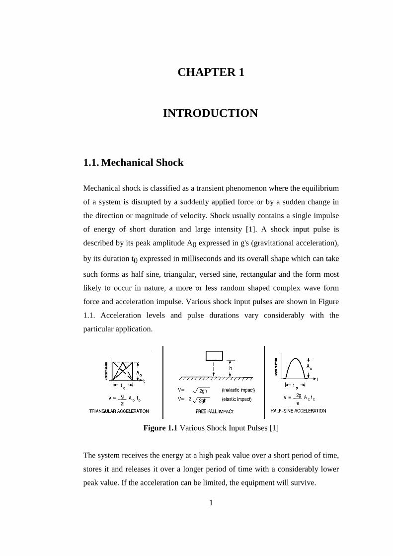
Mechanical shock is classified as a transient phenomenon where the equilibrium
of a system is disrupted by a suddenly applied force or by a sudden change in
the direction or magnitude of velocity. Shock usually contains a single impulse
of energy of short duration and large intensity [1]. A shock input pulse is
described by its peak amplitude A0 expressed in g's (gravitational acceleration),
by its duration t0 expressed in milliseconds and its overall shape which can take
such forms as half sine, triangular, versed sine, rectangular and the form most
likely to occur in nature, a more or less random shaped complex wave form
force and acceleration impulse. Various shock input pulses are shown in Figure
1.1. Acceleration levels and pulse durations vary considerably with the
particular application.
Figure 1.1 Various Shock Input Pulses [1]
The system receives the energy at a high peak value over a short period of time,
stores it and releases it over a longer period of time with a considerably lower
peak value. If the acceleration can be limited, the equipment will survive.
2
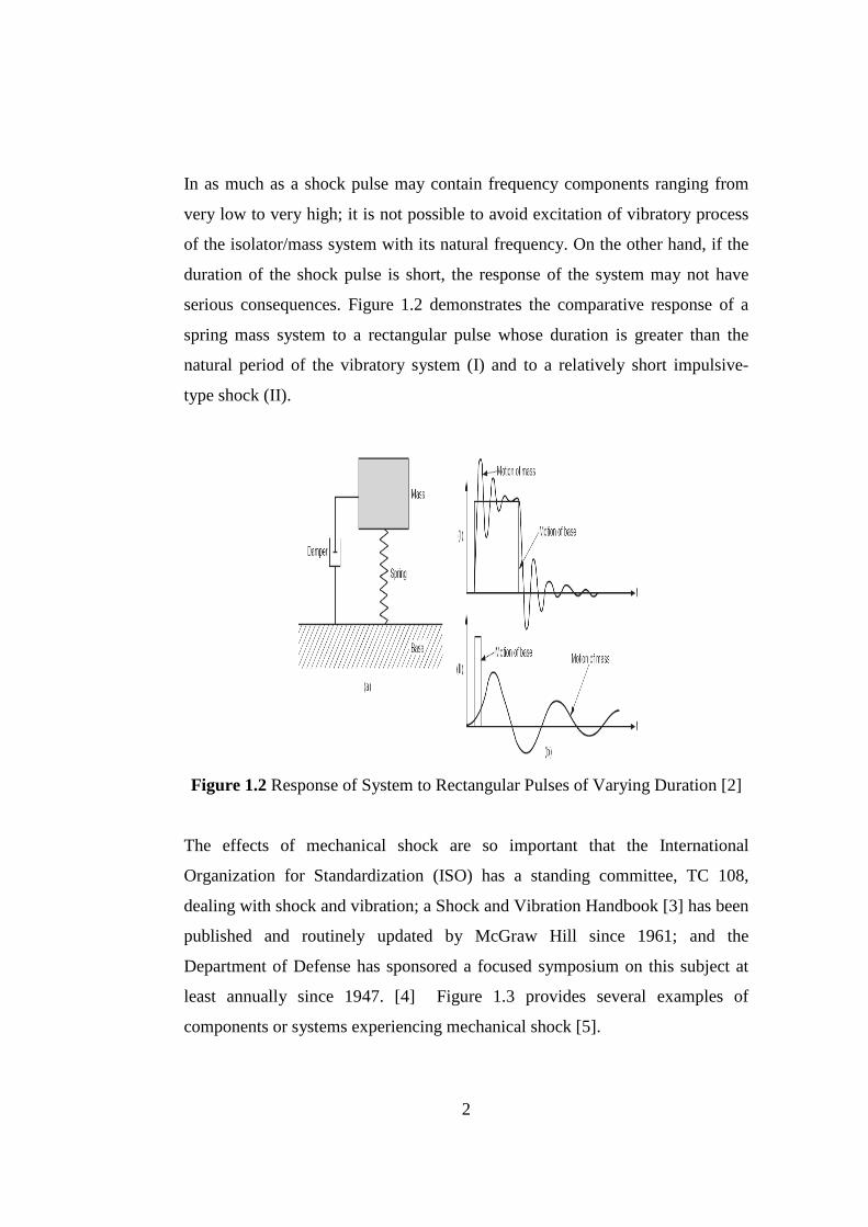
In as much as a shock pulse may contain frequency components ranging from
very low to very high; it is not possible to avoid excitation of vibratory process
of the isolator/mass system with its natural frequency. On the other hand, if the
duration of the shock pulse is short, the response of the system may not have
serious consequences. Figure 1.2 demonstrates the comparative response of a
spring mass system to a rectangular pulse whose duration is greater than the
natural period of the vibratory system (I) and to a relatively short impulsive-
type shock (II).
Figure 1.2 Response of System to Rectangular Pulses of Varying Duration [2]
The effects of mechanical shock are so important that the International
Organization for Standardization (ISO) has a standing committee, TC 108,
dealing with shock and vibration; a Shock and Vibration Handbook [3] has been
published and routinely updated by McGraw Hill since 1961; and the
Department of Defense has sponsored a focused symposium on this subject at
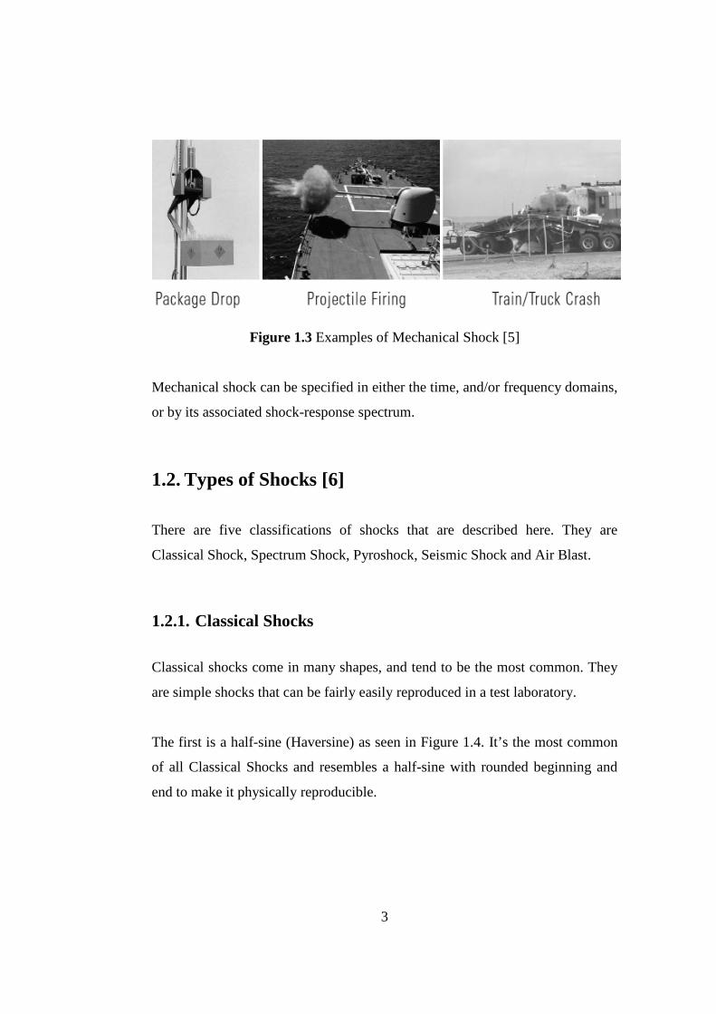
least annually since 1947. [4] Figure 1.3 provides several examples of
components or systems experiencing mechanical shock [5].
3
Figure 1.3 Examples of Mechanical Shock [5]
Mechanical shock can be specified in either the time, and/or frequency domains,
or by its associated shock-response spectrum.
1.2. Types of Shocks [6]
There are five classifications of shocks that are described here. They are
Classical Shock, Spectrum Shock, Pyroshock, Seismic Shock and Air Blast.
1.2.1. Classical Shocks
Classical shocks come in many shapes, and tend to be the most common. They
are simple shocks that can be fairly easily reproduced in a test laboratory.
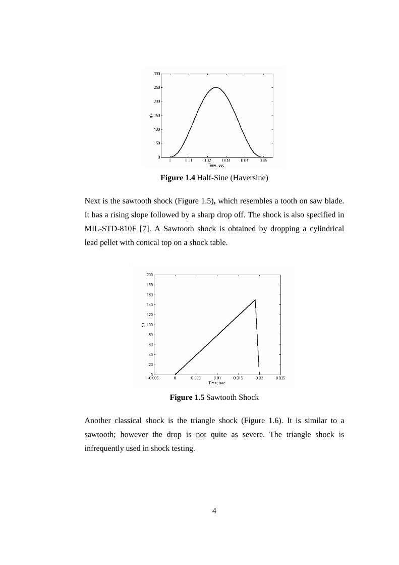
The first is a half-sine (Haversine) as seen in Figure 1.4. It’s the most common
of all Classical Shocks and resembles a half-sine with rounded beginning and
end to make it physically reproducible.
4
Figure 1.4 Half-Sine (Haversine)
Next is the sawtooth shock (Figure 1.5), which resembles a tooth on saw blade.
It has a rising slope followed by a sharp drop off. The shock is also specified in
MIL-STD-810F [7]. A Sawtooth shock is obtained by dropping a cylindrical
lead pellet with conical top on a shock table.
Figure 1.5 Sawtooth Shock
Another classical shock is the triangle shock (Figure 1.6). It is similar to a
sawtooth; however the drop is not quite as severe. The triangle shock is
infrequently used in shock testing.

5
Figure 1.6 Triangle Shock
1.2.2. Spectrum Shock
A shock response spectrum defined by frequency and acceleration level pairs
and uses the Shock Response Spectrum (SRS) for measurement. (Figure 1.7)
Figure 1.7 Shock Spectrum
1.2.3. Pyroshock
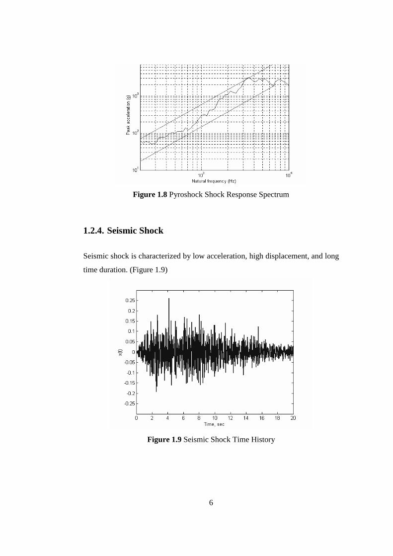
Pyroshock is characterized by a high acceleration, short duration shock pulse
Pyroshock also uses the SRS for measurement. (Figure 1.8)
6
Figure 1.8 Pyroshock Shock Response Spectrum
1.2.4. Seismic Shock
Seismic shock is characterized by low acceleration, high displacement, and long
time duration. (Figure 1.9)
Figure 1.9 Seismic Shock Time History
7
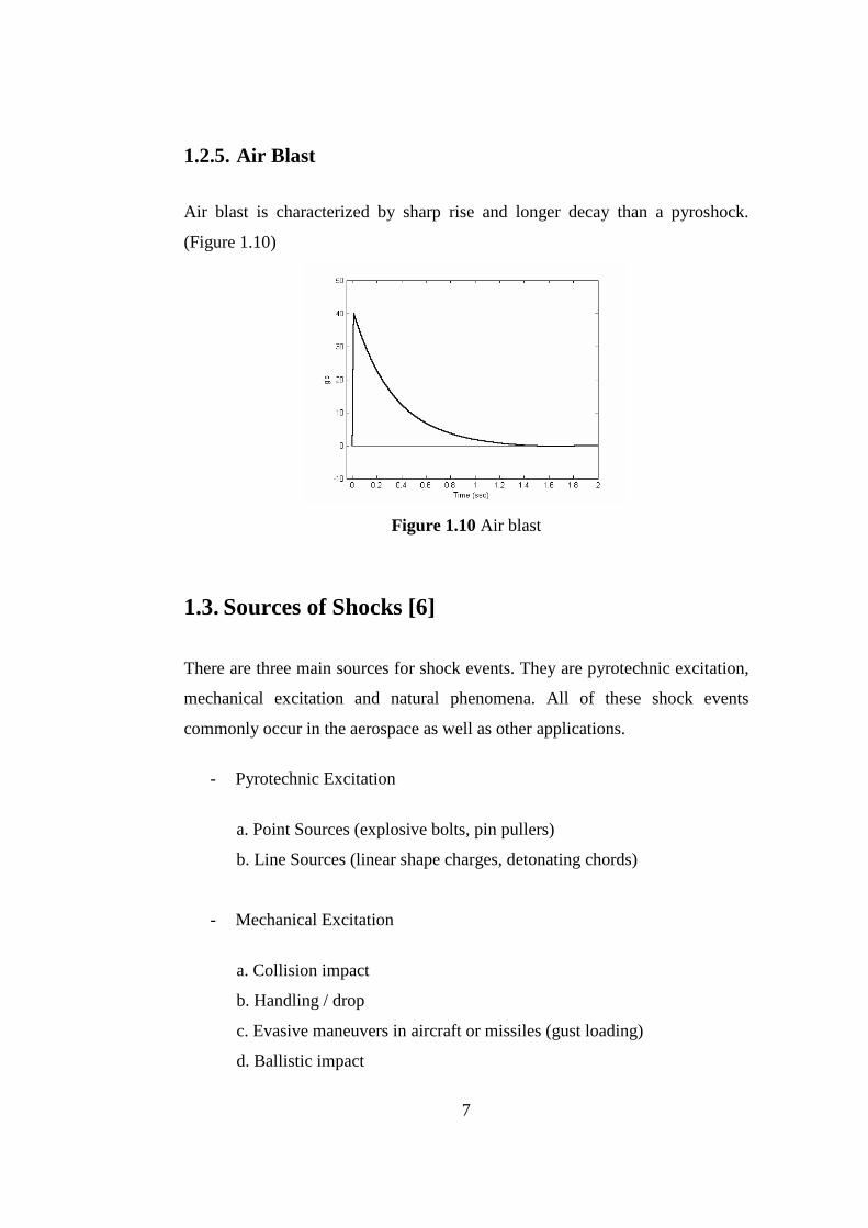
1.2.5. Air Blast
Air blast is characterized by sharp rise and longer decay than a pyroshock.
(Figure 1.10)
Figure 1.10 Air blast
1.3. Sources of Shocks [6]
There are three main sources for shock events. They are pyrotechnic excitation,
mechanical excitation and natural phenomena. All of these shock events
commonly occur in the aerospace as well as other applications.
- Pyrotechnic Excitation
a. Point Sources (explosive bolts, pin pullers)
b. Line Sources (linear shape charges, detonating chords)
- Mechanical Excitation
a. Collision impact
b. Handling / drop
c. Evasive maneuvers in aircraft or missiles (gust loading)
d. Ballistic impact
8
e. Aircraft landing
f. Braking
g. Missile / Rocket launching
h. Gunfire
i. High-speed fluid entry
j. Transportation, uneven surfaces, rough terrain
- Natural Phenomenon
a. Earthquake
b. Wind gust
c. Air blast
d. Ocean waves
e. Ice impact
1.4. Shock Testing Methods [6]
Shock testing is commonly performed by the following methods. Each method
imparts the kinetic energy to the system in a different manner.
• Drop
• Hammer / Impact
• Shaker (Electrodynamic / Hydraulic)
• Pyroshock
• Hopkinson Bar
In drop testing ∆V≠0 (change in velocity) and ∆d≠0 (change in displacement),
while others maintain zero overall change in velocity and displacement. Further
details can be found in [6].
9
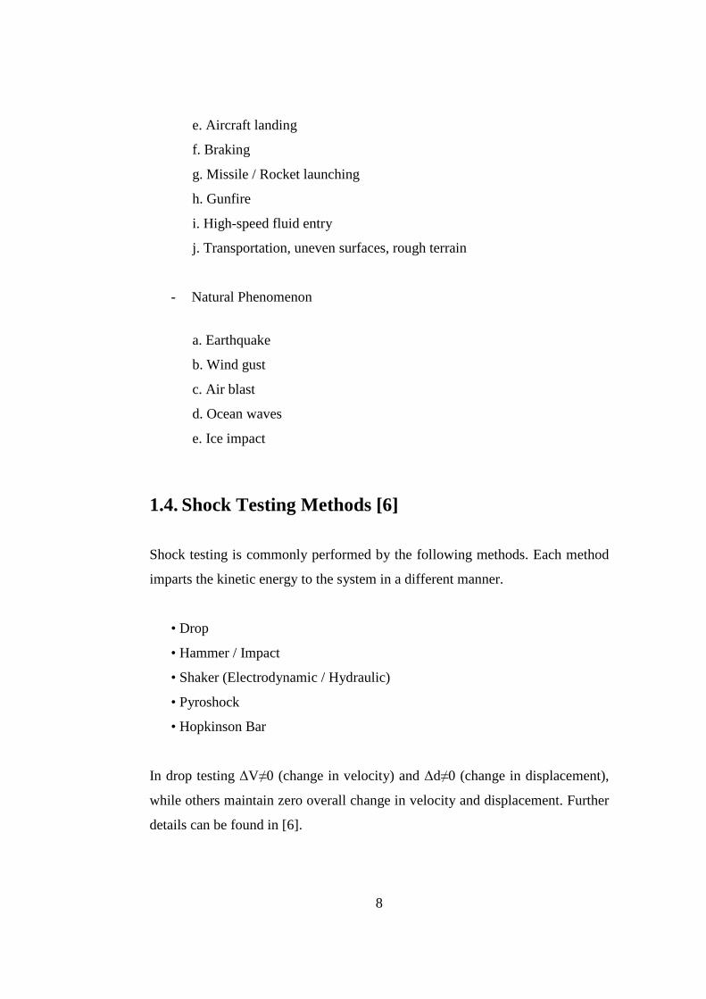
1.5. Overview of the Study
Shocks can cause structural failures such as cracked hausings, fatigue cracks,
deformation of structures [6], etc. In this study, the shock induced transient
stress analysis of the test pieces for a Gatling gun and the 25mm cannon mount
will be performed to investigate their structural failure (yielding). Test pieces
and the mount of 25mm cannon are integrated on the gun and the cannon
respectively. Test pieces are not the part of the Gatling gun system. They are
just used to obtain data and observe the shock failure without deformation on
the system. Application of the pieces and the 25mm cannon mount on the
systems are shown in Figure 1.11 to Figure 1.13.
Figure 1.11 Application of a Test Piece on Gatling Gun
Test Piece
Gatling Gun
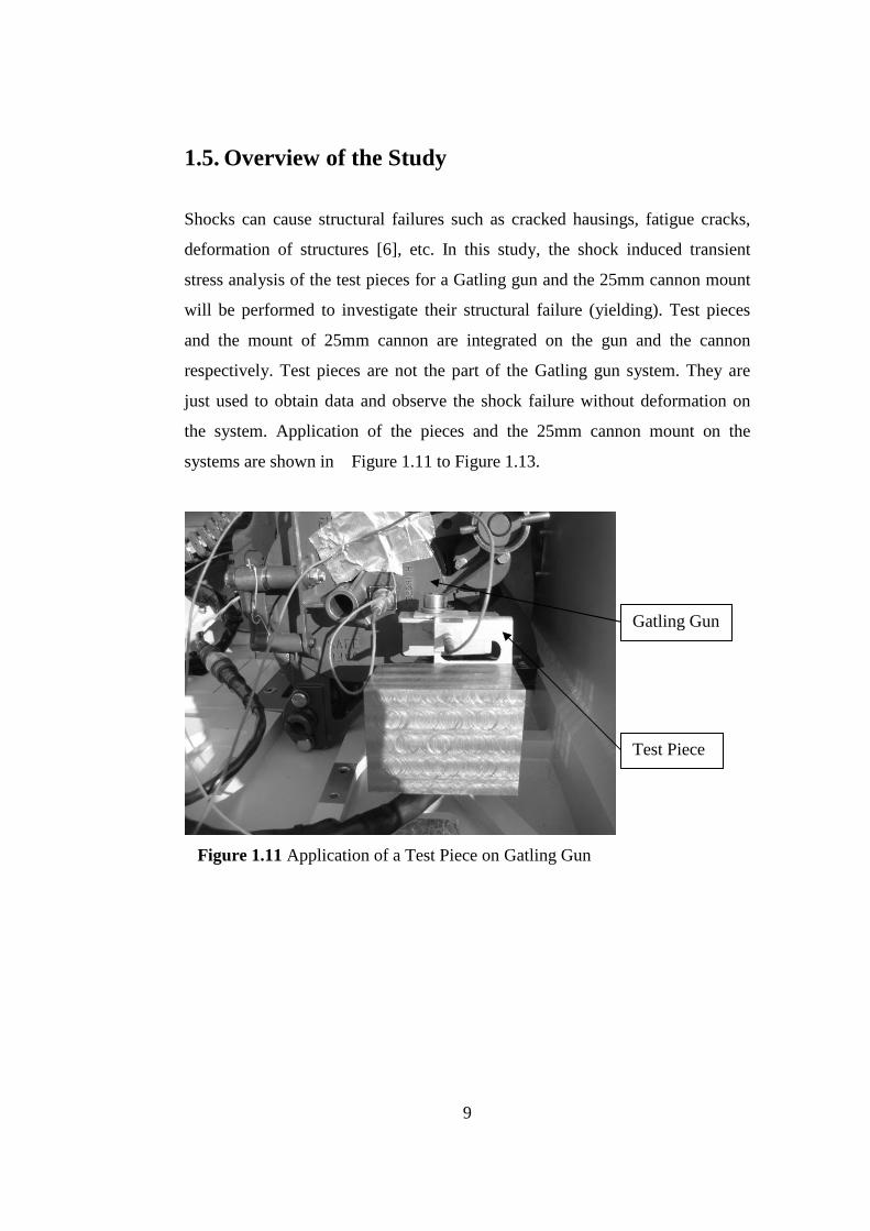
10
Figure 1.12 A Test Piece used for Experimental Analysis
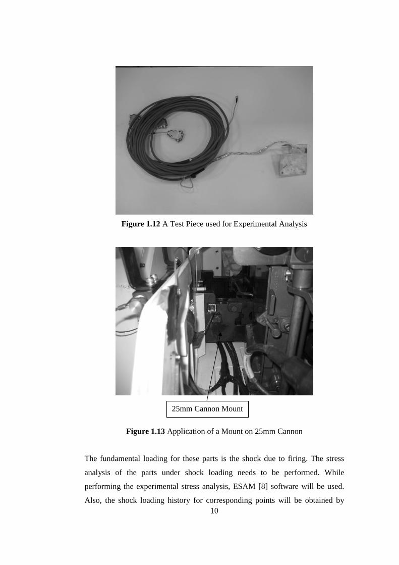
Figure 1.13 Application of a Mount on 25mm Cannon
The fundamental loading for these parts is the shock due to firing. The stress
analysis of the parts under shock loading needs to be performed. While
performing the experimental stress analysis, ESAM [8] software will be used.
Also, the shock loading history for corresponding points will be obtained by
25mm Cannon Mount
11
using ICP (integrated circuit piezoelectric) [9] accelerometers. Shock Response
Spectrum (SRS) analysis (nCode Glypworks) [10] will be done to define the
equivalent shock profiles by using the obtained shock loading history.
Since the implementation of actual shock loading in Finite Element Analysis
takes too much computational time, an equivalent classical shock (Haversine) is
used.
After that, transient shock analysis will be performed to find the numerical
stress values. Numerical and experimental stress values will be compared to
verify the finite element models (FEM). Finally the stress and strain energy
density values will be used to define which values give more accurate results to
define the effect of shock loading on the parts. The details of these studies will
be explained in the following chapters.
12
CHAPTER 2
2. LITERATURE SURVEY
The shock loading problem under consideration in this study is a complex one
due to the following factors:
- It is a rapid phenomenon that excites dynamic (resonant) response of the
material but it causes very little overall deflection,
- It causes multiaxial stress state.
- In a comparatively short time, a moderately high level force impulse is
input to the material.
Shock Response Spectrum (SRS) analysis was developed as a standard data
processing method in the early 1960’s. Firstly SRS was used by U.S.
Department of Defense. Now this signal processing method is standardized by
ISO 18431-4 [11]. Detailed information on SRS is given in Chapter 3.
A brief review of some studies which are related to the work done in this study
is given below.
Biot et al. [12] conceived the shock response spectrum. He defined the SRS as
the maximum response motion from a set of single DOF oscillators covering the
frequency range. He showed how to pick a small number of modes which are
adequate for design. For earthquake applications, he used the traditional
assumption that the ground’s motion is not affected by the dynamic motion of
the building. Later another study demonstrated that this assumption is overly
conservative and leads to over design of equipment. He noted that frequency
peaks in shock spectra from a single earthquake are not constant within the
13
same neighborhood. This led to recommending an envelope approach of all
spectra for design purposes. Relative to loadings on buildings, he found that
stresses calculated using the maximum envelope approach was much higher
than those observed from an actual earthquake. He attributed this to factors such
as damping, plastic deformation, and possible interaction of nearby soil with the
foundation of the building.
Housner et al. [13] developed the first spectra used for seismic design of
structures in the late 1950s. These were obtained by averaging and smoothing
the response spectra from eight ground motion records, two from each of the
following four earthquakes.
- El Centro (1934)
- El Centro (1940)
- Olympia (1949)
- Tekiachapi (1952)
Newmark et al. [14] presented a family of single-step integration methods for
the solution of structural dynamic problems for both blast and seismic loading.
During the past 40 years Newmark’s method has been applied to the dynamic
analysis of many practical engineering structures. In addition, it has been
modified and improved by many other researchers.
Newmark et al. [15] developed an earthquake design spectrum approach based
on amplification factors applied to maximum ground motions. The
amplification factors are listed for different probabilities of occurrence and also
for various levels of damping of the structure. He showed how a spectrum is
developed from the ground motion maxima. The region of amplified response is
between the relatively high and relatively low frequency extremes of the
spectrum. At relatively high frequencies, the shock spectrum level approached
the maximum ground acceleration. This is the aforementioned feature that was
observed in the earlier El Centro earthquake.

14
Kelly and Richman et al. [16] clarified physical descriptions and mathematical
presentation of the shock response spectrum (SRS). This article has been cited
in multiple handbooks on the subject and research articles. The main purpose of
this note was to correct several typographical errors in the Biot manuscript’s
presentation of a recursive algorithm for SRS calculations. These errors were
consistent across all three editions of the monograph. The secondary purpose of
this note was to present a Matlab implementation of the corrected algorithm.
Justin, Andrew and Winfred et al. [17] verified the corrections described in the
preceding [16] by comparing the corrected algorithm and the original algorithm
to an independent SRS code. The independent code used a piecewise-linear
approximation for the base acceleration. The various algorithms were applied to
accelerometer data from the ignition environment of live-fire testing of the
Space Shuttle Reusable Solid Rocket Motor. Specifically, data was evaluated
from the radial channel at station 1479.5 on Technical Evaluation Motor 13.
The data was sampled at 10,000 Hz. The SRS of this acceleration data was
calculated using three different algorithms. The corrected algorithm of
equations was compared with the uncorrected equations from Kelly and
Richman as well as the independent code. For each algorithm, a damping ratio
of ζ = 0.05 was used, and the peak response was calculated for a range of
natural frequencies at one-third octaves up to the Nyquist frequency. The
corrected algorithm and the independent code showed strong agreement with
each other; however, the uncorrected algorithm displayed large differences in
the high frequency regime.
Walter et al. [18] initially clarified what mechanical shock is and why we
measure it. After that, basic requirements are provided for all measurement
systems that process transient signals. High-frequency and low-frequency
dynamic models for a measuring accelerometer were presented and justified.
These models are then used to investigate accelerometer responses to
mechanical shock. The results enabled “rules of thumb” to be developed for

15
shock data assessment and proper accelerometer selection. Other helpful
considerations for measuring mechanical shock were also provided.
Alexander et al. [19] provided a basic overview, or primer, of the shock
response spectrum (SRS). This paper was prepared for the design engineers who
needed to work with the shock response spectrum, and would like to understand
the underlying detail.
Smith and Melander et al. [20] described a study that examined some of the
critical parameters that effect Shock Response Spectrum (SRS) results and
reported on their use by some of the practitioners in the field. They showed that
parameters such as anti-alias filter characteristics, ac-coupling strategies, and
analysis algorithm/strategy can strongly effect the results and that they are not
uniformly applied by system suppliers or users.
Hollowell and Smith et al. [21] discussed the problem further and presents an
analytical procedure that may be applied to achieve agreement between the data
sets acquired and analyzed by different laboratories.
Tuma and Koci et al. [22] presented the method of calculation of the shock
response spectrum, which was corresponding to an acceleration signal exciting
the resonance vibration of substructures. SRS determined the maximum or
minimum of the substructure acceleration response as a function of the natural
frequencies of a set of the single degree of freedom systems modeling the
mentioned substructures. The shock was recorded in digital form, commonly as
acceleration signal. The single-degree-of-freedom systems (SDOF) were
approximated by an IIR digital filter and the filter response to the sampled
acceleration signal was easily calculated. This shock response spectrum shows
how the individual component of the impulse signal excites the mechanical
structure to resonate.

16
Çelik [23] used experimental approach to perform the failure analysis of the
launcher assembly of a military land vehicle. Finite element analysis was
performed to determine the critical locations where strain rosettes were settled
down on the physical prototype. Tests were carried out by performing
operational life profile of the vehicle in the field. Absolute maximum principal
stresses were determined at each rosette location by analyzing the strain data
collected. At the study, functional failures of the electronic equipments in the
system are investigated.
Çelik et al. [24] applied shock and vibration control techniques using spring
isolators to provide dynamic protection of the system units installed on the
vehicles. The Repetitive Shock Response Spectrum (SRS) analysis was
performed to define the gunfire vibration profile and make qualification that the
electronic equipments should withstand. It was also intended to obtain required
stabilization during operation of the platform.
Douglas et al. [25] examined recent efforts attempted to improve the simulation
results of the athwartship (transversely across a ship from one side to the other)
motion including shock spectra analysis, and the reasons behind the disparities
that exist between the simulated values and the actual trial data. He thought that
shock spectra analysis could serve as a design tool as well as a tool for
comparative analysis. Barge testing were used to shock qualify naval equipment
for years, yet using these UNDEX simulations and the shock spectra’s created,
accurate predictions of the frequency response can be achieved. As a
comparative tool, the shock spectra showed that the low frequency response is
very accurately modeled, and in many cases the simulations are more
conservative than the actual trial data.
Parlak et al. [26] did the experimental analysis of repetitive recoil shocks due to
machine gun firing. The machine gun was located on the military Low Level
17
Air Defence System. For the test of shock and vibration on the system, four
different points were determined and ICP (integrated circuit piezoelectric)
accelerometers were located for corresponding points. Shock Response
Spectrum (SRS) analysis was done to define the minimum shock profile that the
electronic equipments should withstand. It was aimed to use these equivalent
simple shock profiles during the shock qualification testing of the equipments.
Rusovici et al. [27] employed high-damping viscoelastic materials in the design
of geometrically complex impact absorbent components. The Anelastic
Displacement Fields (ADF) method was employed to develop new
axisymmetric and plane stress finite elements that were capable of modeling
frequency dependent material behavior of linear viscoelastic materials. The new
finite elements were used to model and analyze behavior of viscoelastic
structures subjected to shock loads. The development of such ADF-based finite
element models offered an attractive analytical tool to aid in the design of shock
absorbent mechanical filters. This work also showed that it is possible to
determine material properties’ frequency dependence by iteratively fitting ADF
model predictions to experimental results.
Carpinteri et al. [28] carried out a study on expected principal stress directions
under multiaxial loading. A theoretical procedure to calculate the Euler angles
from the matrix of the principal direction cosines for a generic time instant was
proposed. The procedure consists of averaging the instantaneous values of the
three Euler angles through weight functions. It was examined how such
theoretical principal directions determined by applying the proposed procedure
are correlated to the position of the experimental fracture plane for some fatigue
tests in the literature. The algorithm proposed is applied to some experimental
biaxial in- and out-of-phase stress states to assess the correlation. From the
results obtained, it was seen that in the case of a small phase angle, the normal
vector to the experimental fracture plane agrees with the expected direction of
the maximum principal stress.

18
Shang et al. [29] developed a new theory for the application of local stress-
strain field intensity to the fatigue damage at a notch. The effects of the local
stress-strain gradient on fatigue damage were taken into account at notches. The
parameters needed for local stress-strain intensity approach, as a fatigue analysis
tool, were calculated from an incremental elastic-plastic finite element analysis
under random cyclic loading.
Consequently, critical conditions and important outcomes found in the literature
are noted to be considered in this study. No studies which are directly related
with the shock failure (yielding) analysis of a mechanical structure by using
SRS could be found.

19
CHAPTER 3
3. THEORIES USED IN THE ANALYSIS
3.1. Shock Response Spectrum Theory
Shock motion in the form of time history is usually not very useful for
engineering purposes. In order to extract useful information, such as the
amount of strain and stress that will be applied on an instrument due to a shock
or to synthesize a shock at laboratory conditions that will have the same
characteristics as that will be experienced in the field, time domain data has to
be reduced to a different form. One of the most commonly used forms of this
reduction is the Shock Response Spectrum (SRS).
Shock response spectrum is the plot of the maximum acceleration of single
degree of freedom (SDOF) systems with different natural frequencies when
excited with a given shock input.
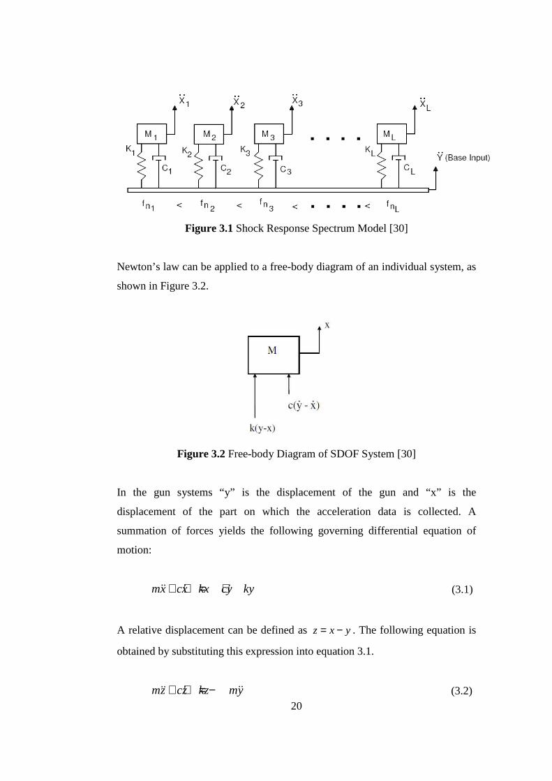
As it was stated above, mechanical shock pulses are analyzed in terms of shock
response spectra. The shock response spectrum assumes that the mechanical
shock pulse is applied as a common base input to a group of independent single-
degree-of freedom systems, see Figure 3.1. The shock response spectrum gives
the peak response of each system with respect to the natural frequency of each
system. Damping is typically fixed at a constant value, such as 5%, which is
equivalent to an amplification factor of Q=10 [30].
20
Figure 3.1 Shock Response Spectrum Model [30]
Newton’s law can be applied to a free-body diagram of an individual system, as
shown in Figure 3.2.
Figure 3.2 Free-body Diagram of SDOF System [30]
In the gun systems “y” is the displacement of the gun and “x” is the
displacement of the part on which the acceleration data is collected. A
summation of forces yields the following governing differential equation of
motion:
mx cx kx cy ky+ + = +ɺɺ ɺ ɺ (3.1)
A relative displacement can be defined as z x y= − . The following equation is
obtained by substituting this expression into equation 3.1.
mz cz kz my+ + = − ɺɺɺɺ ɺ (3.2)
21
Additional substitutions can be made as follows,
2n
k
mω = , 2 n
c
mξω = (3.3), (3.4)
Note that ξ is the damping ratio, and that nω is the natural frequency.
Furthermore, ξ is often represented by the amplification factor Q, where
Q=1/(2 ξ) (3.5)
Substitution of these terms into equation 3.2 yields an equation of motion for
the relative response,
22 ( )n nz z z y tξω ω+ + = −ɺɺɺɺ ɺ (3.6)
Equation 3.6 does not have a closed-form solution for the general case in which
( )y tɺɺ is an arbitrary function. A convolution integral approach must be used to
solve the equation. The convolution integral is then transformed into a series for
the case where ( )y tɺɺ is in the form of digitized data. Furthermore, the series is
converted to a digital recursive filtering relationship (computational process, or
algorithm, transforming a discrete sequence of numbers “the input” into another
discrete sequence of numbers “the output” having a modified frequency domain
spectrum) to expedite the calculation. The resulting formula for the absolute
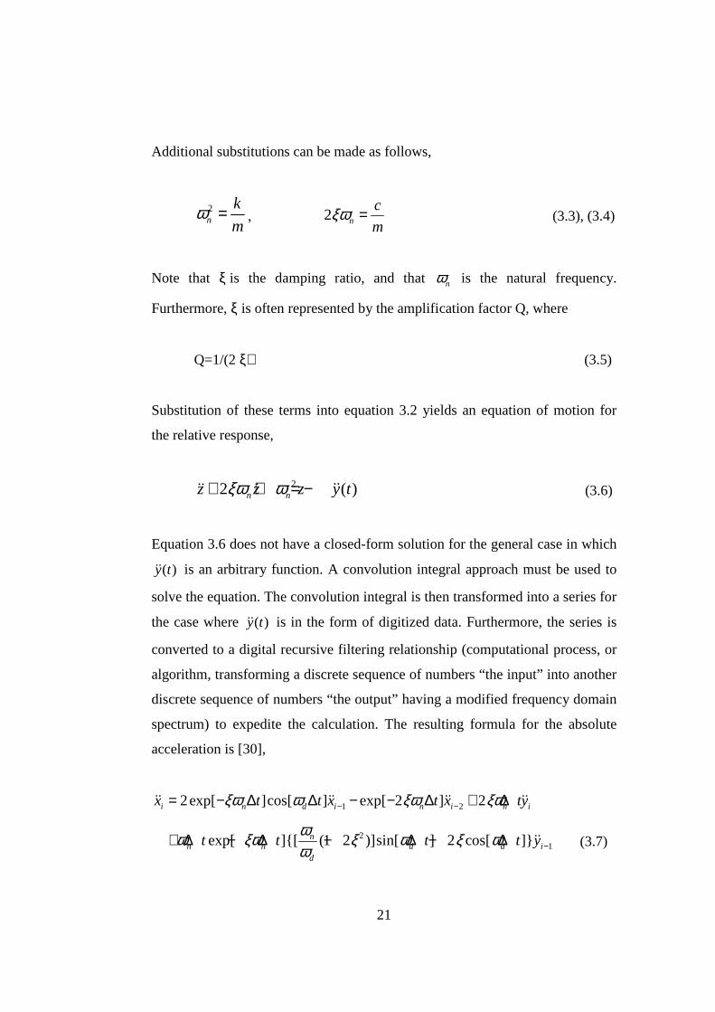
acceleration is [30],
1 22exp[ ]cos[ ] exp[ 2 ] 2i n d i n i n ix t t x t x tyξω ω ξω ξω− −= − ∆ ∆ − − ∆ + ∆ɺɺ ɺɺ ɺɺ ɺɺ
21exp[ ]{[ (1 2 )]sin[ ] 2 cos[ ]}n
n n d d id
t t t t yωω ξω ξ ω ξ ωω −+ ∆ − ∆ − ∆ − ∆ ɺɺ (3.7)
22
where, ω ω ζd n= −1 2 (3.8)
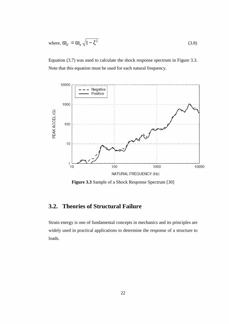
Equation (3.7) was used to calculate the shock response spectrum in Figure 3.3.
Note that this equation must be used for each natural frequency.
Figure 3.3 Sample of a Shock Response Spectrum [30]
3.2. Theories of Structural Failure
Strain energy is one of fundamental concepts in mechanics and its principles are
widely used in practical applications to determine the response of a structure to
loads.

23
3.2.1. Total Strain Energy Theory [31]
The theory, as proposed by Beltrami, and also attributed to Haigh, is based on a
critical value of the total strain energy stored in the material, and this is a
product of stress and strain.
The work done in elastic deformation or the stored elastic strain energy may be
written as,
1
2u W xδ= (3.9)
or,
1122
W x
Ax
δσε= per unit volume (3.10)
In a three-dimensional stress system, the total strain energy is,
1 1 2 2 3 3
1 1 1
2 2 2TU σ ε σ ε σ ε= + + (3.11)
Now using a stress-strain relationship, the principle strains may be written as,
11 2 3( )
E E
σ υε σ σ= − + (3.12)
22 3 1( )
E E
σ υε σ σ= − + (3.13)
33 2 1( )
E E
σ υε σ σ= − + (3.14)
substituting for 1 2 3, ,ε ε ε and rearranging,
2 2 21 2 3 1 2 2 3 3 1
1( ) ( )
2 2TUE E
υσ σ σ σ σ σ σ σ σ= + + − + + (3.15)
24
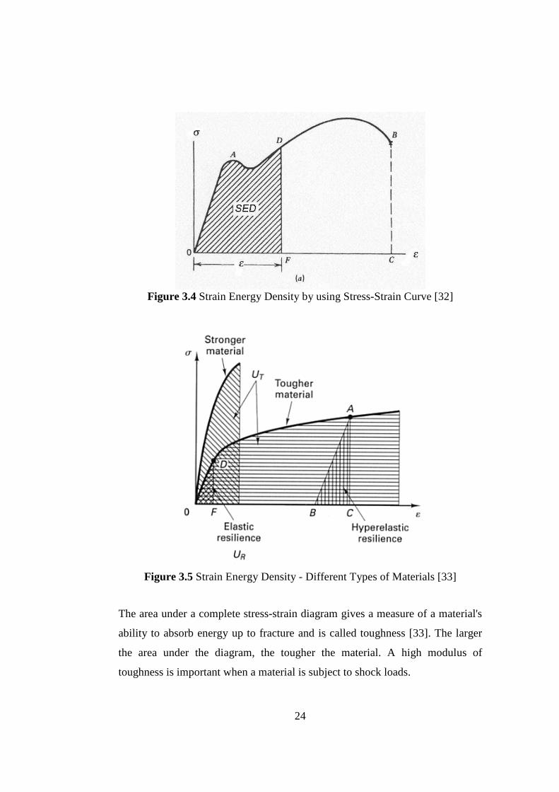
Figure 3.4 Strain Energy Density by using Stress-Strain Curve [32]
Figure 3.5 Strain Energy Density - Different Types of Materials [33]
The area under a complete stress-strain diagram gives a measure of a material's
ability to absorb energy up to fracture and is called toughness [33]. The larger
the area under the diagram, the tougher the material. A high modulus of
toughness is important when a material is subject to shock loads.

25
3.2.2. Distortion Energy Theory [34]
Huber, in 1904, proposed that the total strain energy of an element of material
could be divided into two parts, that due to change in volume and that due to
change in shape. These will be termed volumetric strain energy UV, and
distortion or shear strain energy, US. It is rather more simple to determine the
former quantity then the latter, and since the total strain energy has already been
determined, the shear or distortion component can be determined as,
US = UT – UV (3.16)
The distortion energy theory says that failure (yielding) occurs due to distortion
of a part, not due to volumetric changes in the part (shearing causes distortion).
Failure will occur if,
3132212
32
22
1' σσσσσσσσσσ −−−++= ≥ Sy (3.17)
In terms of applied stresses,
( ) ( ) ( ) ( )σ
σ σ σ σ σ σ τ τ τ' =
− + − + − + + +x y y z z xy xy yz zx
2 2 2 2 2 26
2 (3.18)
σ ’ is called the Von Mises effective stress.
The distortion energy theory is used in the simulations of the thesis since
ANSYS which is the program used for the simulations applies this theory.
3.2.3. Plastic Deformation [43]
From mechanics point of view, when tensile load is applied to a specimen of
ductile metal, extension of the specimen will occur and specimen will return to
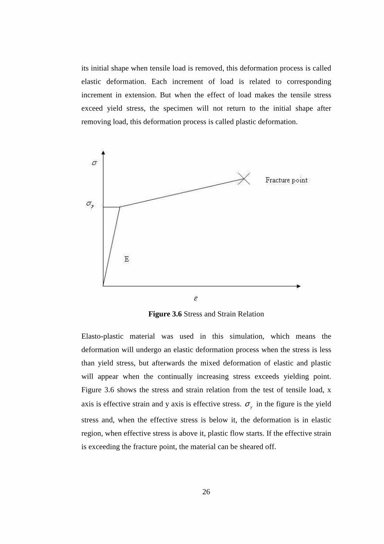
26
its initial shape when tensile load is removed, this deformation process is called
elastic deformation. Each increment of load is related to corresponding
increment in extension. But when the effect of load makes the tensile stress
exceed yield stress, the specimen will not return to the initial shape after
removing load, this deformation process is called plastic deformation.
Figure 3.6 Stress and Strain Relation
Elasto-plastic material was used in this simulation, which means the
deformation will undergo an elastic deformation process when the stress is less
than yield stress, but afterwards the mixed deformation of elastic and plastic
will appear when the continually increasing stress exceeds yielding point.
Figure 3.6 shows the stress and strain relation from the test of tensile load, x
axis is effective strain and y axis is effective stress. yσ in the figure is the yield
stress and, when the effective stress is below it, the deformation is in elastic
region, when effective stress is above it, plastic flow starts. If the effective strain
is exceeding the fracture point, the material can be sheared off.
27
Work hardening is the strengthening of a material by plastic deformation. As the
material becomes increasingly saturated with new dislocations, more
dislocations are prevented from nucleating (a resistance to dislocation-formation
develops). This resistance to dislocation-formation manifests itself as a
resistance to plastic deformation; hence, the observed strengthening.
In metallic crystals, irreversible deformation is usually carried out on a
microscopic scale by defects called dislocations. At normal temperatures the
dislocations are not annihilated by annealing. Instead, the dislocations
accumulate, interact with one another, and serve as pinning points or obstacles
that significantly impede their motion. This leads to an increase in the yield
strength of the material and a subsequent decrease in ductility.
For hardening materials, the yield surface will evolve in space in one of three
ways. The first form of yield surface evolution is called isotropic hardening. For
isotropic hardening, the yield surface grows in size while the center remains at a
fixed point in stress space. The second form of surface evolution is called
kinematic hardening. For kinematic hardening, the center of the yield surface
translates in stress space, while the size remains fixed. The third type of surface
evolution is called mixed hardening where both isotropic and kinematic
hardening characteristics are evident. For mixed hardening, the orientation of
the yield surface may also change as well. Although isotropic hardening is the
most common form of yield surface evolution assumed in finite element models
for metal forming simulation, it is not necessarily the most accurate. The mixed
hardening model is most likely the most accurate of the three models.
28
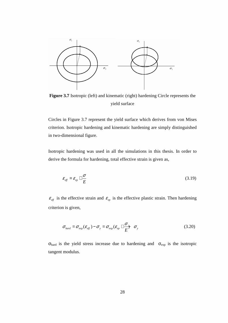
Figure 3.7 Isotropic (left) and kinematic (right) hardening Circle represents the
yield surface
Circles in Figure 3.7 represent the yield surface which derives from von Mises
criterion. Isotropic hardening and kinematic hardening are simply distinguished
in two-dimensional figure.
Isotropic hardening was used in all the simulations in this thesis. In order to
derive the formula for hardening, total effective strain is given as,
eff ep E
σε ε= + (3.19)
effε is the effective strain and epε is the effective plastic strain. Then hardening
criterion is given,
exp exp( ) ( )hard eff y ep yE
σσ σ ε σ σ ε σ= − = + − (3.20)
σhard is the yield stress increase due to hardening and σexp is the isotropic
tangent modulus.
29
3.3 Transient Response Analysis [36]
Structural systems are very often subjected to transient excitation. A transient
excitation is a highly dynamic, time-dependent force exerted on the solid or
structure, such as earthquake, impact and shocks. The discrete governing
equation system for such a structure often requires a special solver. The widely
used method is the so-called direct integration method. The direct integration
method basically uses the finite difference method for time stepping to solve the
system equation. There are two main types of direct integration method: implicit
and explicit.
Explicit methods do not involve the solution of a set of linear equations at each
time step. Basically, these methods use the differential equation at time “t” to
predict a solution at time “t + ∆t”. For most real structures, which contain stiff
elements, a very small time step is required in order to obtain a stable solution.
Therefore, all explicit methods are conditionally stable with respect to the size
of the time step.
On the other hand, implicit methods attempt to satisfy the differential equation
at time “t” after the solution at time “t - ∆t” is found. These methods require the
solution of a set of linear equations at each time step; however, larger time steps
may be used. Implicit methods can be conditionally or unconditionally stable.
There exist a large number of accurate, higher-order, multi-step methods that
have been developed for the numerical solution of differential equations. These
multistep methods assume that the solution is a smooth function in which the
higher derivatives are continuous. The exact solution of many nonlinear
structures requires that the accelerations, the second derivative of the
displacements, are not smooth functions. This discontinuity of the acceleration
is caused by the nonlinear hysteresis of most structural materials, contact
between parts of the structure, and buckling of elements.
30
It is the conclusion [36] that only single-step, implicit, unconditionally stable
methods can be used for the step-by-step shock analysis of the structures.
Before discussing the equations used for the time stepping techniques, it should
be mentioned that the general system equation for a structure can be re-written
as,
KD CD MD F+ + =ɺ ɺɺ (3.21)
Where Dɺ is the vector of velocity components, and C is the matrix of damping
coefficients that are determined experimentally. The ANSYS program uses the
Newmark time integration method to solve these equations at discrete time
points.
3.3.1. Newmark’s Method [35]
Newmark’s method is the most widely used implicit algorithm. It is first
assumed that
2 1( ) ( ) [( ) ]
2t t t t t t tD D t D t D Dβ β+∆ +∆= + ∆ + ∆ − +ɺ ɺɺ ɺɺ (3.22)
( )[(1 ) ]t t t t t tD D t D Dγ γ+∆ +∆= + ∆ − +ɺ ɺ ɺɺ ɺɺ (3.23)
where β and γ are constants. Equations (3.22) and (3.23) are then substituted
into the system equation (3.21),
2 1{ ( ) ( ) [( ) ]} { ( )[(1 ) ]}
2t t t t t t t t t t t t tK D t D t D D C D t D D MD Fβ β γ γ+∆ +∆ +∆ +∆+ ∆ + ∆ − + + + ∆ − + + =ɺ ɺɺ ɺɺ ɺ ɺɺ ɺɺ ɺɺ
(3.24)

31
It is grouped all the terms involving t tD +∆ɺɺ on the left and shift the remaining
terms to the right,
residualcm t t t tK D F+∆ +∆=ɺɺ (3.25)
where,
2[ ( ) ]cmK K t C t Mβ γ= ∆ + ∆ + (3.26)
2 1{ ( ) ( ) ( ) } { ( )(1 ) }
2residual
t t t t t t t t tF F K D t D t D C D t Dβ γ+∆ +∆= − + ∆ + ∆ − − + ∆ −ɺ ɺɺ ɺ ɺɺ (3.27)
The accelerations t tD +∆ɺɺ can then be obtained by solving matrix system equation,
1 residualt t cm t tD K F−+∆ +∆=ɺɺ (3.28)
Newmark’s method, like most implicit methods, is unconditionally stable if γ ≥
0.5 and 2(2 1) /16yβ ≥ + . Unconditionally stable methods are those in which the
size of the time step,t∆ , will not affect the stability of the solution, but rather it
is governed by accuracy considerations. The unconditional stability property
allows the implicit algorithms to use significantly larger time steps when the
external excitation is of a slow time variation.

32
CHAPTER 4
4. FIRING TESTS AND DATA ACQUISITION
The tests are performed for acceleration data acquisition at the mounting
location and stress histories of specific locations. In Figure 4.1 and Figure 4.2,
the systems are shown during the firing tests.
Figure 4.1 A View of Stabilized GAU19/A 12.7mm Gatling Gun System
Figure 4.2 A View of Stabilized KBA 25mm Cannon System
33
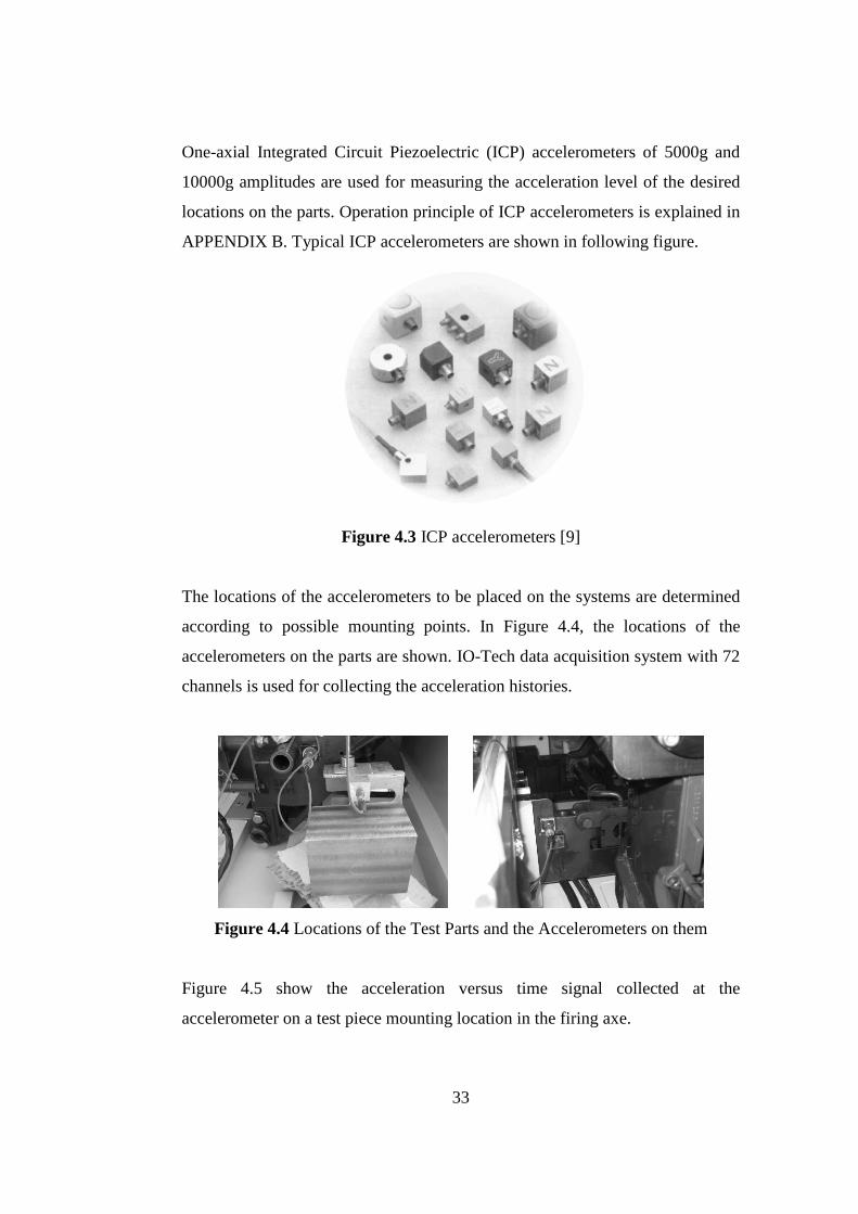
One-axial Integrated Circuit Piezoelectric (ICP) accelerometers of 5000g and
10000g amplitudes are used for measuring the acceleration level of the desired
locations on the parts. Operation principle of ICP accelerometers is explained in
APPENDIX B. Typical ICP accelerometers are shown in following figure.
Figure 4.3 ICP accelerometers [9]
The locations of the accelerometers to be placed on the systems are determined
according to possible mounting points. In Figure 4.4, the locations of the
accelerometers on the parts are shown. IO-Tech data acquisition system with 72
channels is used for collecting the acceleration histories.
Figure 4.4 Locations of the Test Parts and the Accelerometers on them
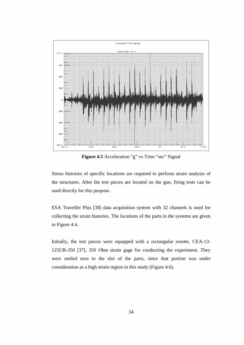
Figure 4.5 show the acceleration versus time signal collected at the
accelerometer on a test piece mounting location in the firing axe.
34
Figure 4.5 Acceleration “g” vs Time “sec” Signal
Stress histories of specific locations are required to perform strain analysis of
the structures. After the test pieces are located on the gun, firing tests can be
used directly for this purpose.
ESA Traveller Plus [38] data acquisition system with 32 channels is used for
collecting the strain histories. The locations of the parts in the systems are given
in Figure 4.4.
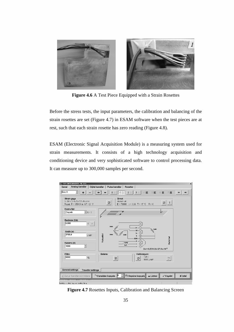
Initially, the test pieces were equipped with a rectangular rosette, CEA-13-
125UR-350 [37], 350 Ohm strain gage for conducting the experiment. They
were settled next to the slot of the parts, since that portion was under
consideration as a high strain region in this study (Figure 4.6).
35
Figure 4.6 A Test Piece Equipped with a Strain Rosettes
Before the stress tests, the input parameters, the calibration and balancing of the
strain rosettes are set (Figure 4.7) in ESAM software when the test pieces are at
rest, such that each strain rosette has zero reading (Figure 4.8).
ESAM (Electronic Signal Acquisition Module) is a measuring system used for
strain measurements. It consists of a high technology acquisition and
conditioning device and very sophisticated software to control processing data.
It can measure up to 300,000 samples per second.
Figure 4.7 Rosettes Inputs, Calibration and Balancing Screen
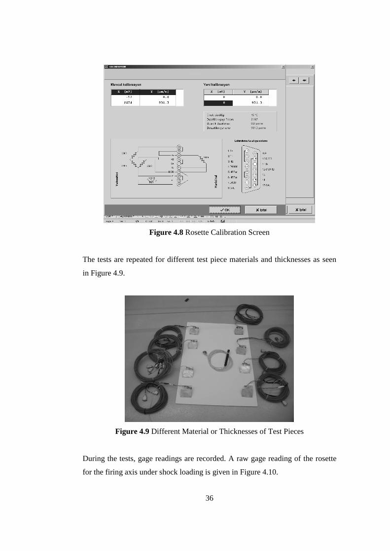
36
Figure 4.8 Rosette Calibration Screen
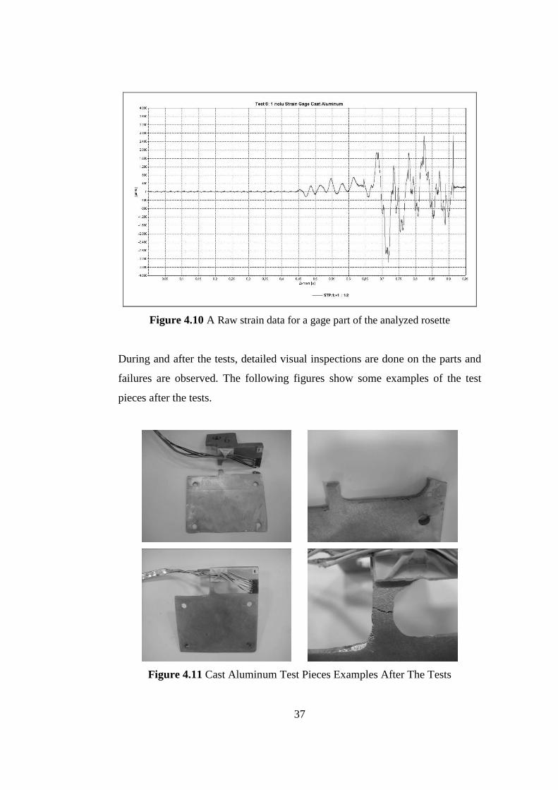
The tests are repeated for different test piece materials and thicknesses as seen
in Figure 4.9.
Figure 4.9 Different Material or Thicknesses of Test Pieces
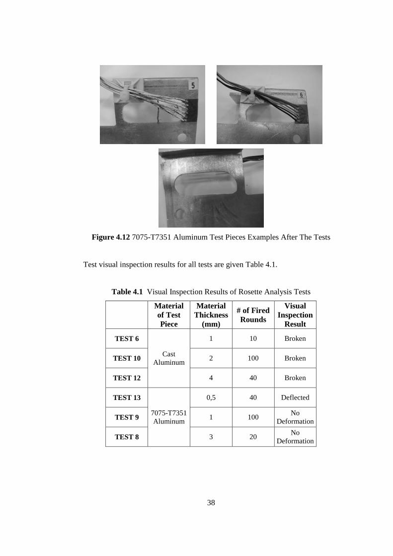
During the tests, gage readings are recorded. A raw gage reading of the rosette
for the firing axis under shock loading is given in Figure 4.10.
37
Figure 4.10 A Raw strain data for a gage part of the analyzed rosette
During and after the tests, detailed visual inspections are done on the parts and
failures are observed. The following figures show some examples of the test
pieces after the tests.
Figure 4.11 Cast Aluminum Test Pieces Examples After The Tests
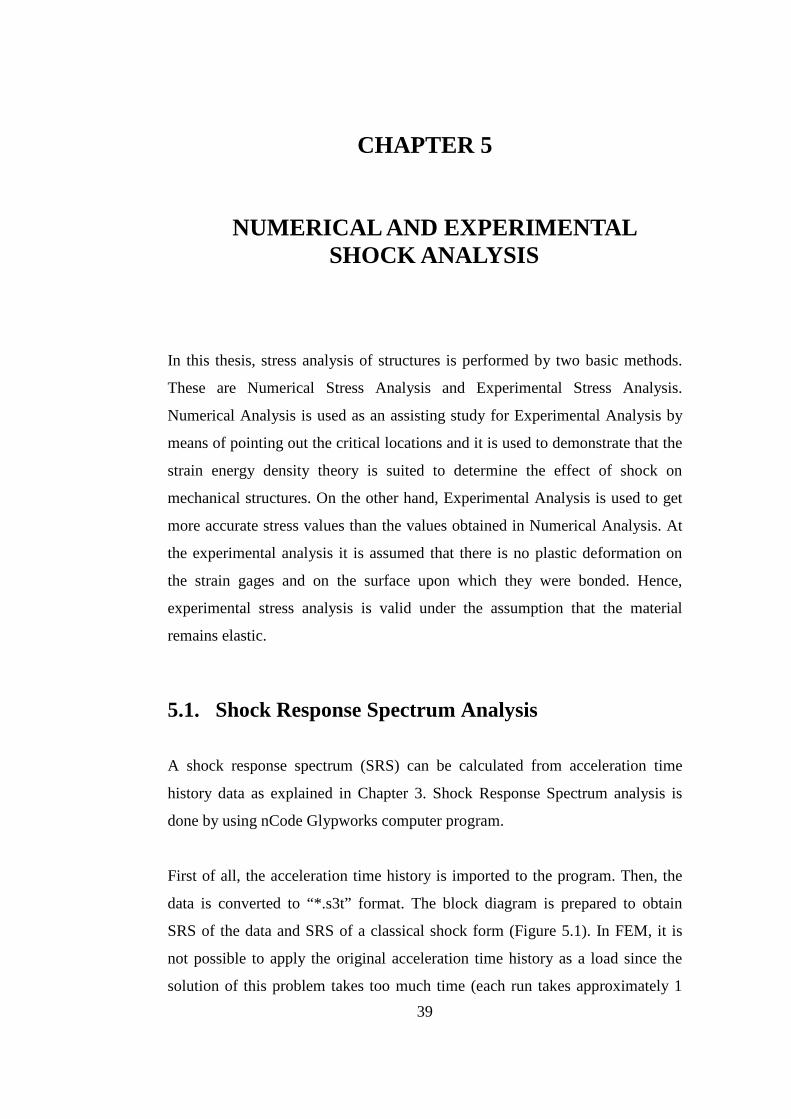
38
Figure 4.12 7075-T7351 Aluminum Test Pieces Examples After The Tests
Test visual inspection results for all tests are given Table 4.1.
Table 4.1 Visual Inspection Results of Rosette Analysis Tests
Material of Test Piece
Material Thickness
(mm)
# of Fired Rounds
Visual Inspection
Result
TEST 6
Cast Aluminum
1 10 Broken
TEST 10 2 100 Broken
TEST 12 4 40 Broken
TEST 13
7075-T7351 Aluminum
0,5 40 Deflected
TEST 9 1 100 No
Deformation
TEST 8 3 20 No
Deformation
39
CHAPTER 5
5. NUMERICAL AND EXPERIMENTAL SHOCK ANALYSIS
In this thesis, stress analysis of structures is performed by two basic methods.
These are Numerical Stress Analysis and Experimental Stress Analysis.
Numerical Analysis is used as an assisting study for Experimental Analysis by
means of pointing out the critical locations and it is used to demonstrate that the
strain energy density theory is suited to determine the effect of shock on
mechanical structures. On the other hand, Experimental Analysis is used to get
more accurate stress values than the values obtained in Numerical Analysis. At
the experimental analysis it is assumed that there is no plastic deformation on
the strain gages and on the surface upon which they were bonded. Hence,
experimental stress analysis is valid under the assumption that the material
remains elastic.
5.1. Shock Response Spectrum Analysis
A shock response spectrum (SRS) can be calculated from acceleration time
history data as explained in Chapter 3. Shock Response Spectrum analysis is
done by using nCode Glypworks computer program.
First of all, the acceleration time history is imported to the program. Then, the
data is converted to “*.s3t” format. The block diagram is prepared to obtain
SRS of the data and SRS of a classical shock form (Figure 5.1). In FEM, it is
not possible to apply the original acceleration time history as a load since the
solution of this problem takes too much time (each run takes approximately 1

40
month on Z400 HP workstation). Hence it is tried to obtain a classical shock
form which supplies approximately the same effects of the original data as a
load in FEM.
Figure 5.1 SRS Block Diagram
The SRS of the classical shock form should be as close as possible to the SRS
of the original data . To obtain this, different types, amplitudes and times of
classical forms are tried.
The general rules for the SRS graphs are;
• If the amplitude of the shock form is constant and the time of the shock
form increases, the graph shifts to the left and the peak value does not
change.
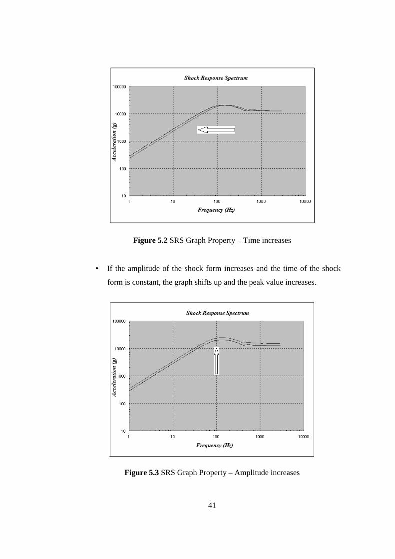
41
Figure 5.2 SRS Graph Property – Time increases
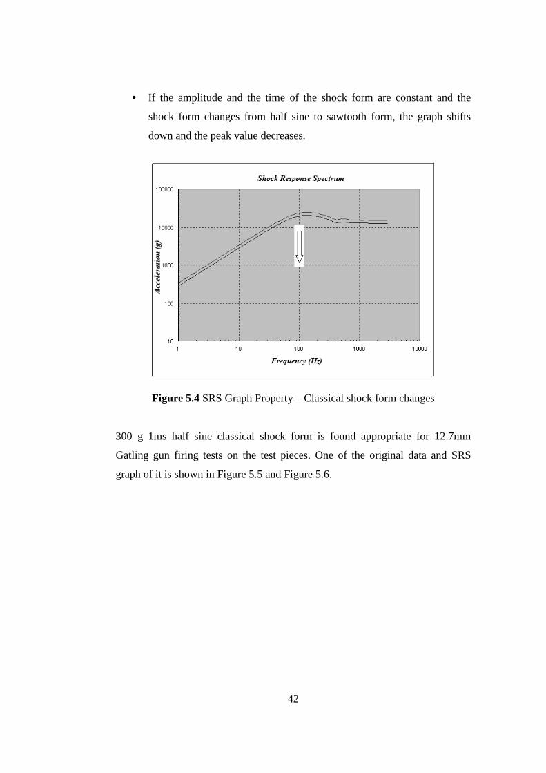
• If the amplitude of the shock form increases and the time of the shock
form is constant, the graph shifts up and the peak value increases.
Figure 5.3 SRS Graph Property – Amplitude increases
42
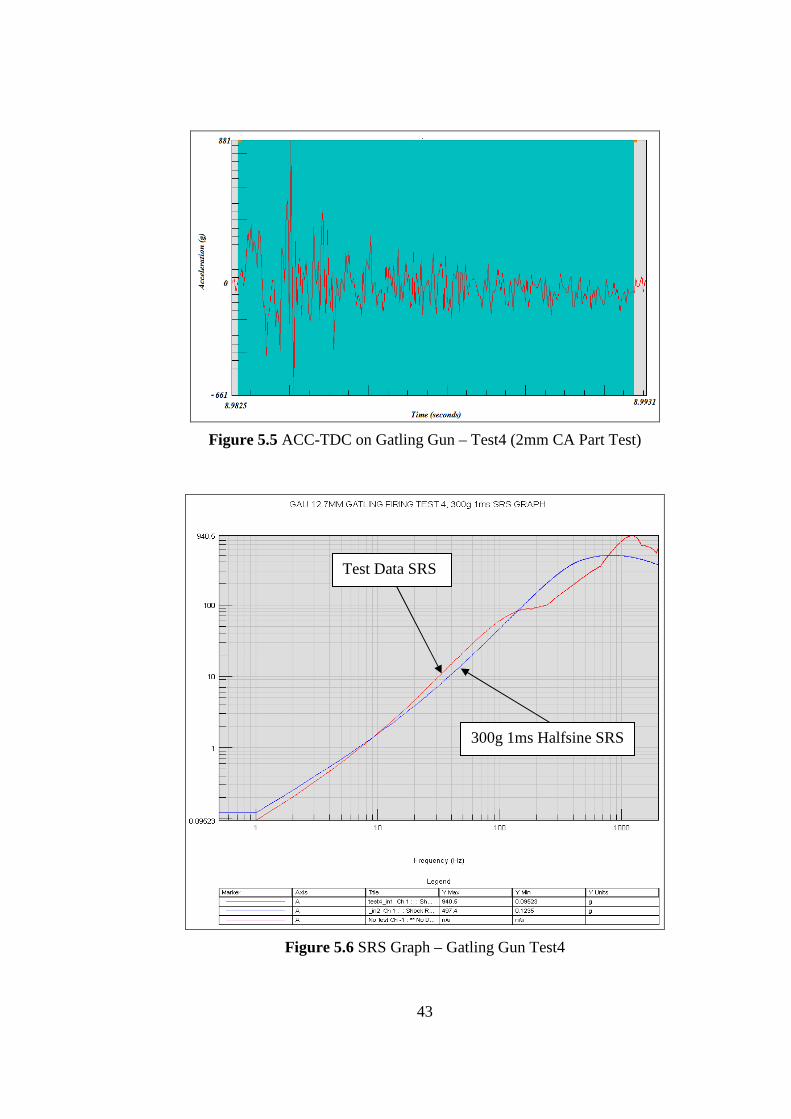
• If the amplitude and the time of the shock form are constant and the
shock form changes from half sine to sawtooth form, the graph shifts
down and the peak value decreases.
Figure 5.4 SRS Graph Property – Classical shock form changes
300 g 1ms half sine classical shock form is found appropriate for 12.7mm
Gatling gun firing tests on the test pieces. One of the original data and SRS
graph of it is shown in Figure 5.5 and Figure 5.6.
43
Figure 5.5 ACC-TDC on Gatling Gun – Test4 (2mm CA Part Test)
Figure 5.6 SRS Graph – Gatling Gun Test4
Test Data SRS
300g 1ms Halfsine SRS
44
5.2. Experimental Stress Analysis
Experimental analysis is essential since the results of it are nearly exact (in the
elastic range) and are used to be compared with the finite element model results.
After the gage readings as explained in Chapter 4, rosette analysis is performed.
Brief information on experimental stress analysis and rosette calculations is
given in APPENDIX C.
ESAM (Electronic Signal Acquisition Module) software is also used for the
experimental stress analysis.
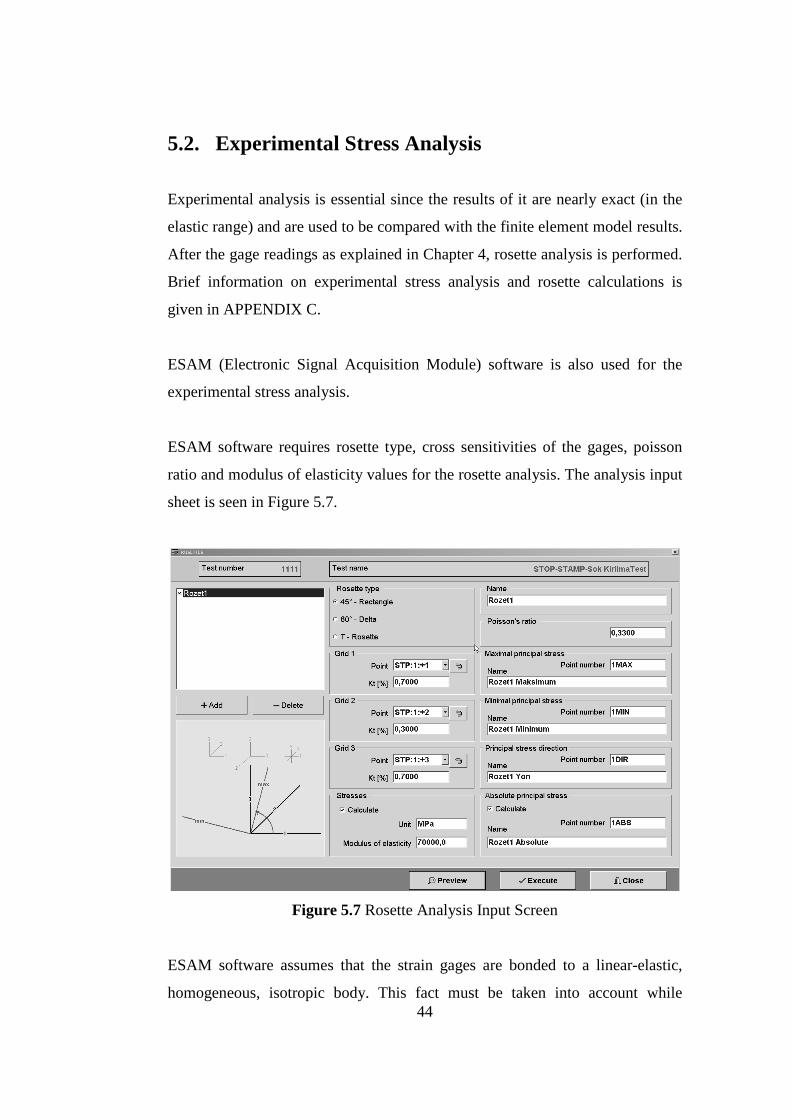
ESAM software requires rosette type, cross sensitivities of the gages, poisson
ratio and modulus of elasticity values for the rosette analysis. The analysis input
sheet is seen in Figure 5.7.
Figure 5.7 Rosette Analysis Input Screen
ESAM software assumes that the strain gages are bonded to a linear-elastic,
homogeneous, isotropic body. This fact must be taken into account while
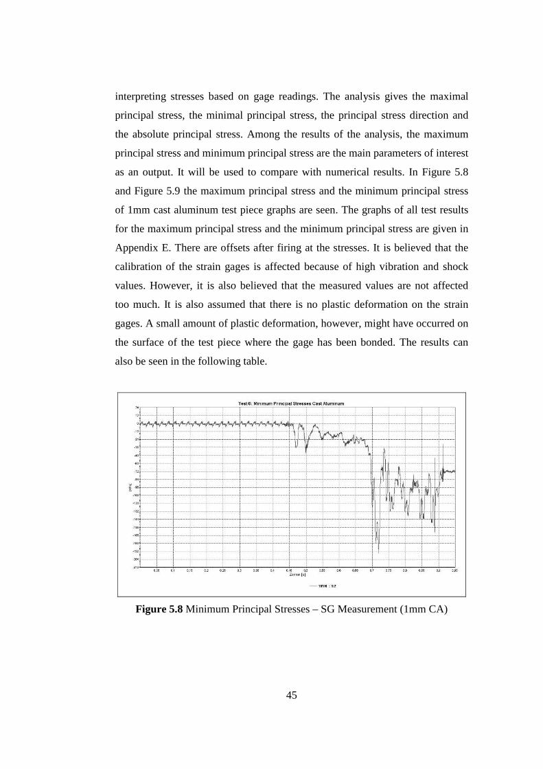
45
interpreting stresses based on gage readings. The analysis gives the maximal
principal stress, the minimal principal stress, the principal stress direction and
the absolute principal stress. Among the results of the analysis, the maximum
principal stress and minimum principal stress are the main parameters of interest
as an output. It will be used to compare with numerical results. In Figure 5.8
and Figure 5.9 the maximum principal stress and the minimum principal stress
of 1mm cast aluminum test piece graphs are seen. The graphs of all test results
for the maximum principal stress and the minimum principal stress are given in
Appendix E. There are offsets after firing at the stresses. It is believed that the
calibration of the strain gages is affected because of high vibration and shock
values. However, it is also believed that the measured values are not affected
too much. It is also assumed that there is no plastic deformation on the strain
gages. A small amount of plastic deformation, however, might have occurred on
the surface of the test piece where the gage has been bonded. The results can
also be seen in the following table.
Figure 5.8 Minimum Principal Stresses – SG Measurement (1mm CA)
46
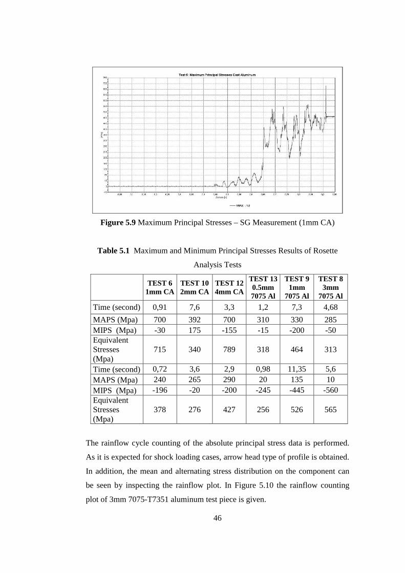
Figure 5.9 Maximum Principal Stresses – SG Measurement (1mm CA)
Table 5.1 Maximum and Minimum Principal Stresses Results of Rosette
Analysis Tests
TEST 6 1mm CA
TEST 10 2mm CA
TEST 12 4mm CA
TEST 13 0.5mm 7075 Al
TEST 9 1mm
7075 Al
TEST 8 3mm
7075 Al Time (second) 0,91 7,6 3,3 1,2 7,3 4,68
MAPS (Mpa) 700 392 700 310 330 285 MIPS (Mpa) -30 175 -155 -15 -200 -50 Equivalent Stresses (Mpa)
715 340 789 318 464 313
Time (second) 0,72 3,6 2,9 0,98 11,35 5,6 MAPS (Mpa) 240 265 290 20 135 10 MIPS (Mpa) -196 -20 -200 -245 -445 -560 Equivalent Stresses (Mpa)
378 276 427 256 526 565
The rainflow cycle counting of the absolute principal stress data is performed.
As it is expected for shock loading cases, arrow head type of profile is obtained.
In addition, the mean and alternating stress distribution on the component can
be seen by inspecting the rainflow plot. In Figure 5.10 the rainflow counting
plot of 3mm 7075-T7351 aluminum test piece is given.
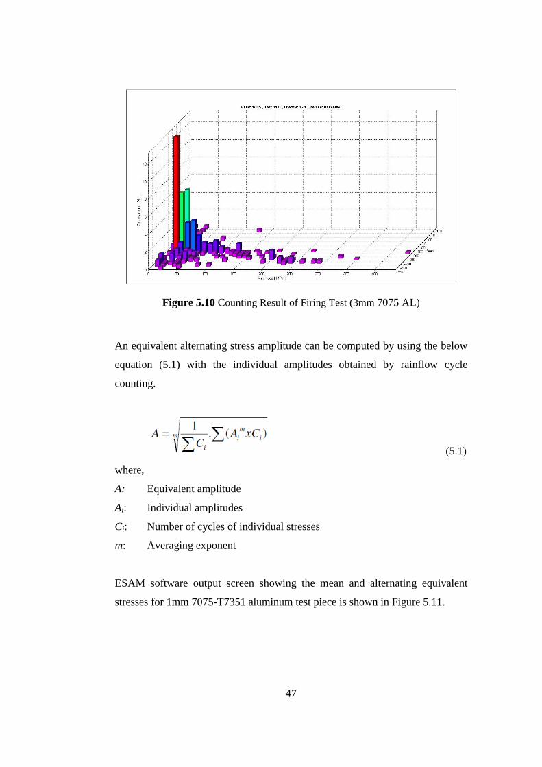
47
Figure 5.10 Counting Result of Firing Test (3mm 7075 AL)
An equivalent alternating stress amplitude can be computed by using the below
equation (5.1) with the individual amplitudes obtained by rainflow cycle
counting.
(5.1)
where,
A: Equivalent amplitude
Ai: Individual amplitudes
Ci: Number of cycles of individual stresses
m: Averaging exponent
ESAM software output screen showing the mean and alternating equivalent
stresses for 1mm 7075-T7351 aluminum test piece is shown in Figure 5.11.
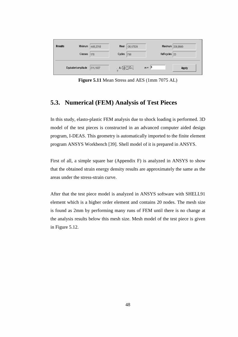
48
Figure 5.11 Mean Stress and AES (1mm 7075 AL)
5.3. Numerical (FEM) Analysis of Test Pieces
In this study, elasto-plastic FEM analysis due to shock loading is performed. 3D
model of the test pieces is constructed in an advanced computer aided design
program, I-DEAS. This geometry is automatically imported to the finite element
program ANSYS Workbench [39]. Shell model of it is prepared in ANSYS.
First of all, a simple square bar (Appendix F) is analyzed in ANSYS to show
that the obtained strain energy density results are approximately the same as the
areas under the stress-strain curve.
After that the test piece model is analyzed in ANSYS software with SHELL91
element which is a higher order element and contains 20 nodes. The mesh size
is found as 2mm by performing many runs of FEM until there is no change at
the analysis results below this mesh size. Mesh model of the test piece is given
in Figure 5.12.

49
Figure 5.12 Mesh Model of the Test Piece
The test piece model contains 2430 SHELL elements and 2620 nodes.
The test pieces are made of 7075-T7351 aluminum or cast aluminum. Material
properties of 7075-T7351 aluminum are found by literature survey and entered
into the material library of ANSYS Workbench as seen in Table 5.2 to Table 5.4
and Figure 5.13. On the other hand, material properties of cast aluminum are
found by tensile test. The information of the test is given in Appendix D. From
Appendix D it is observed that CA behaves in a linear elastic manner until
fracture with UTS=104 MPa and rupture strain=0.0015.
Table 5.2 Material Properties of 7075-T7351 Aluminum
7075-T7351
Elastic Region Engineering Strain (εeng_e) 0,006
Elastic Region Engineering Stress (σeng_e) (MPa) 435
Plastic Region Engineering Strain (εeng_p) 0,13
Plastic Region Engineering Stress (σeng_p) (MPa) 505
Density (kg/mm3) 2,81 x 10⁻⁶
In ANSYS, all stress-strain input should be in terms of true stress and true (or
logarithmic) strain and the results in all outputs are given also as true stress and
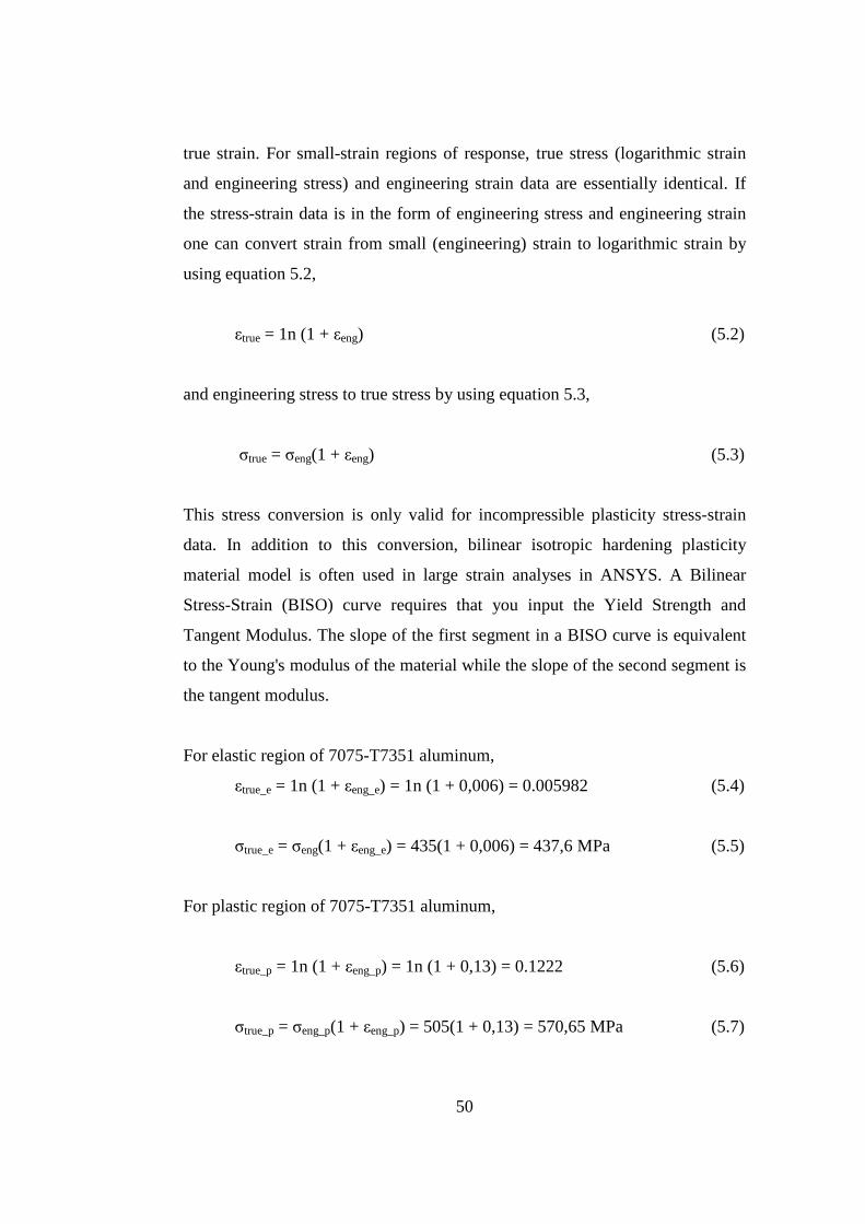
50
true strain. For small-strain regions of response, true stress (logarithmic strain
and engineering stress) and engineering strain data are essentially identical. If
the stress-strain data is in the form of engineering stress and engineering strain
one can convert strain from small (engineering) strain to logarithmic strain by
using equation 5.2,
εtrue = 1n (1 + εeng) (5.2)
and engineering stress to true stress by using equation 5.3,
σtrue = σeng(1 + εeng) (5.3)
This stress conversion is only valid for incompressible plasticity stress-strain
data. In addition to this conversion, bilinear isotropic hardening plasticity
material model is often used in large strain analyses in ANSYS. A Bilinear
Stress-Strain (BISO) curve requires that you input the Yield Strength and
Tangent Modulus. The slope of the first segment in a BISO curve is equivalent
to the Young's modulus of the material while the slope of the second segment is
the tangent modulus.
For elastic region of 7075-T7351 aluminum,
εtrue_e = 1n (1 + εeng_e) = 1n (1 + 0,006) = 0.005982 (5.4)
σtrue_e = σeng(1 + εeng_e) = 435(1 + 0,006) = 437,6 MPa (5.5)
For plastic region of 7075-T7351 aluminum,
εtrue_p = 1n (1 + εeng_p) = 1n (1 + 0,13) = 0.1222 (5.6)
σtrue_p = σeng_p(1 + εeng_p) = 505(1 + 0,13) = 570,65 MPa (5.7)

51
E = σtrue_e / εtrue_e = 73,2 GPa (5.8)
P = (σtrue_p - σtrue_e) / (εtrue_p - εtrue_e) = 1144,8 MPa (5.9)
Table 5.3 Structural Material Properties for 7075-T7351 Al in ANSYS
Young's Modulus 73200 MPa Poisson's Ratio 0,33
Tensile Yield Strength 437,6, MPa
Tensile Ultimate Strength 570,65, MPa
Table 5.4 Bilinear Isotropic Hardening Properties for 7075-T7351 Al in
ANSYS
Yield Strength (MPa) 437,6 Tangent Modulus (MPa) 1144,8
Figure 5.13 Bilinear Isotropic Hardening Graph for 7075-T7351 Al in ANSYS
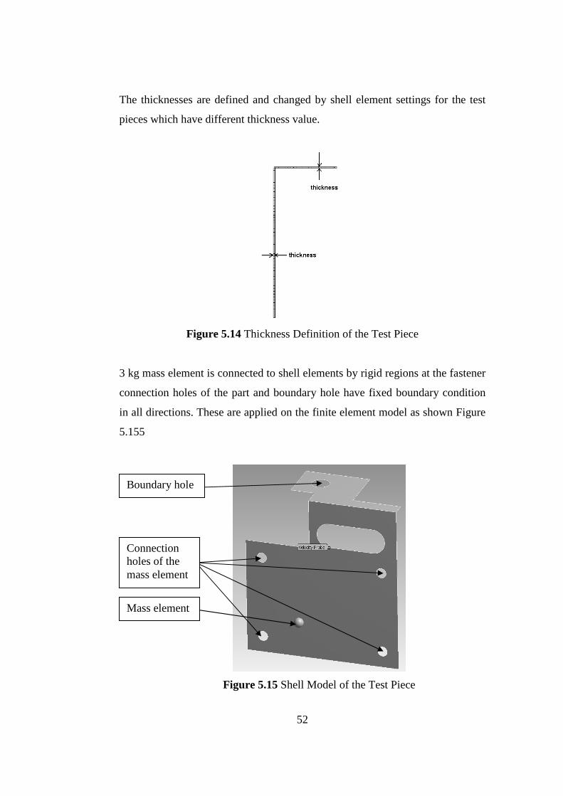
52
The thicknesses are defined and changed by shell element settings for the test
pieces which have different thickness value.
Figure 5.14 Thickness Definition of the Test Piece
3 kg mass element is connected to shell elements by rigid regions at the fastener
connection holes of the part and boundary hole have fixed boundary condition
in all directions. These are applied on the finite element model as shown Figure
5.155
Figure 5.15 Shell Model of the Test Piece
Connection holes of the mass element
Mass element
Boundary hole
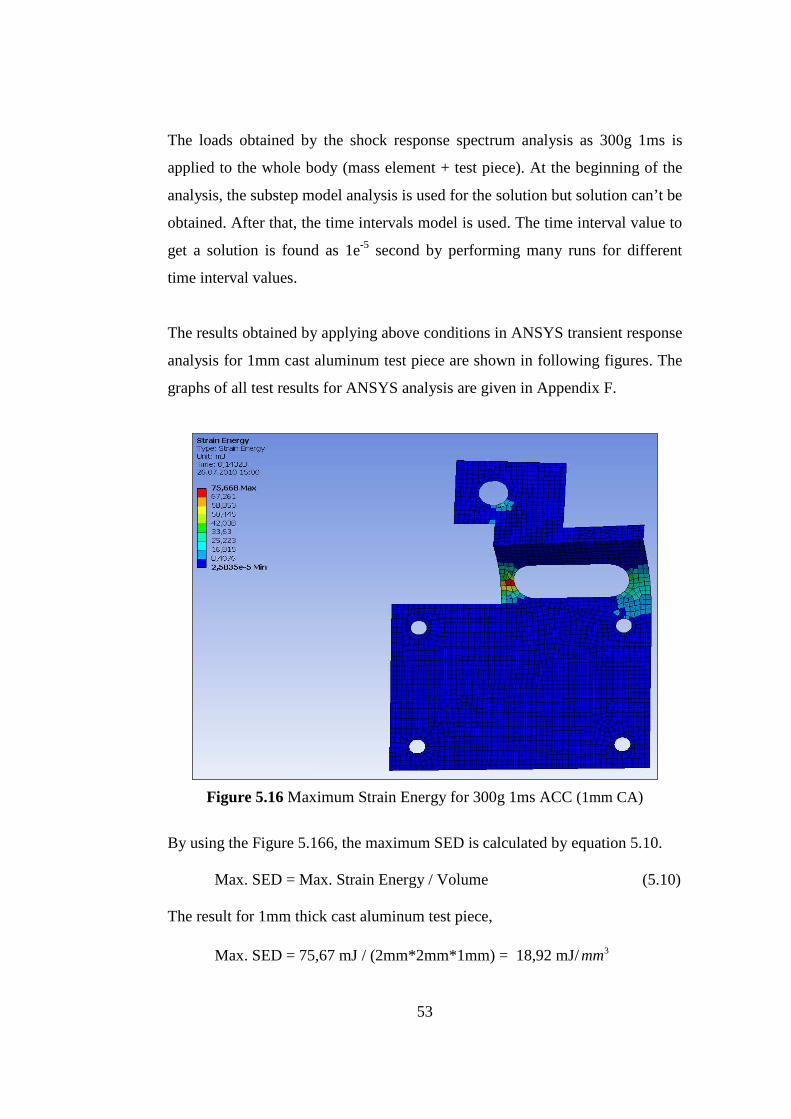
53
The loads obtained by the shock response spectrum analysis as 300g 1ms is
applied to the whole body (mass element + test piece). At the beginning of the
analysis, the substep model analysis is used for the solution but solution can’t be
obtained. After that, the time intervals model is used. The time interval value to
get a solution is found as 1e-5 second by performing many runs for different
time interval values.
The results obtained by applying above conditions in ANSYS transient response
analysis for 1mm cast aluminum test piece are shown in following figures. The
graphs of all test results for ANSYS analysis are given in Appendix F.
Figure 5.16 Maximum Strain Energy for 300g 1ms ACC (1mm CA)
By using the Figure 5.166, the maximum SED is calculated by equation 5.10.
Max. SED = Max. Strain Energy / Volume (5.10)
The result for 1mm thick cast aluminum test piece, Max. SED = 75,67 mJ / (2mm*2mm*1mm) = 18,92 mJ/3mm
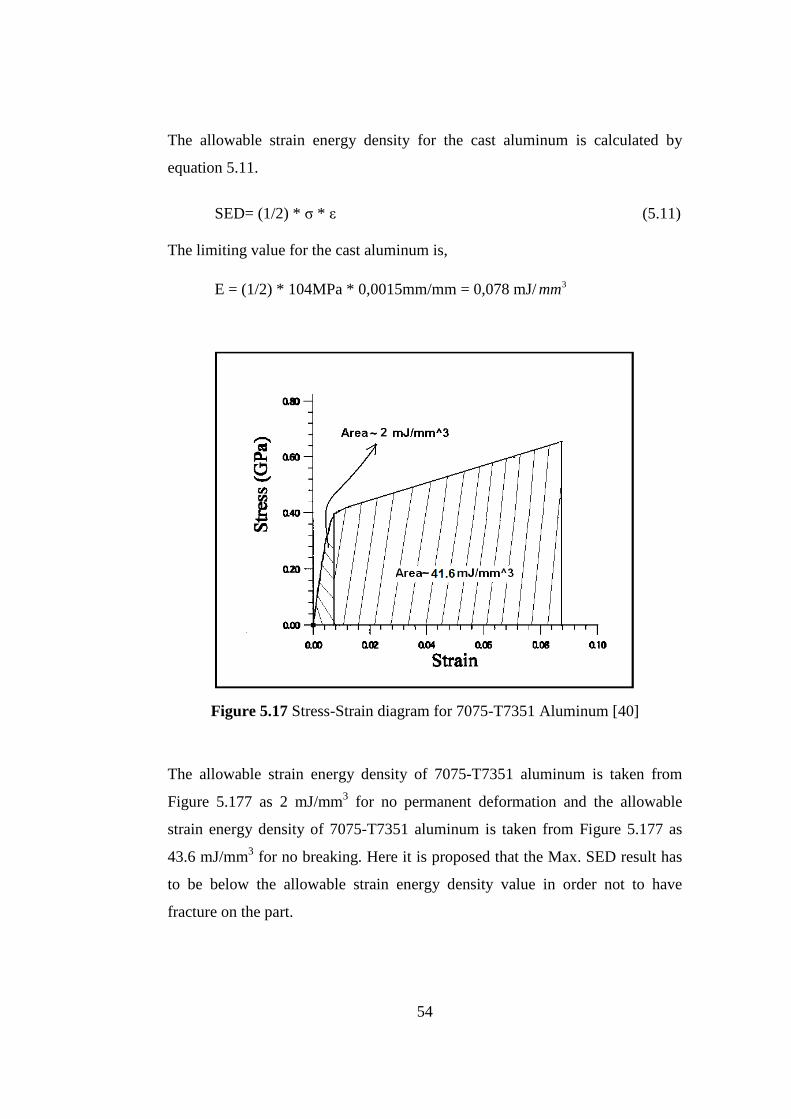
54
The allowable strain energy density for the cast aluminum is calculated by
equation 5.11.
SED= (1/2) * σ * ε (5.11)
The limiting value for the cast aluminum is,
E = (1/2) * 104MPa * 0,0015mm/mm = 0,078 mJ/3mm
Figure 5.17 Stress-Strain diagram for 7075-T7351 Aluminum [40]
The allowable strain energy density of 7075-T7351 aluminum is taken from
Figure 5.177 as 2 mJ/mm3 for no permanent deformation and the allowable
strain energy density of 7075-T7351 aluminum is taken from Figure 5.177 as
43.6 mJ/mm3 for no breaking. Here it is proposed that the Max. SED result has
to be below the allowable strain energy density value in order not to have
fracture on the part.
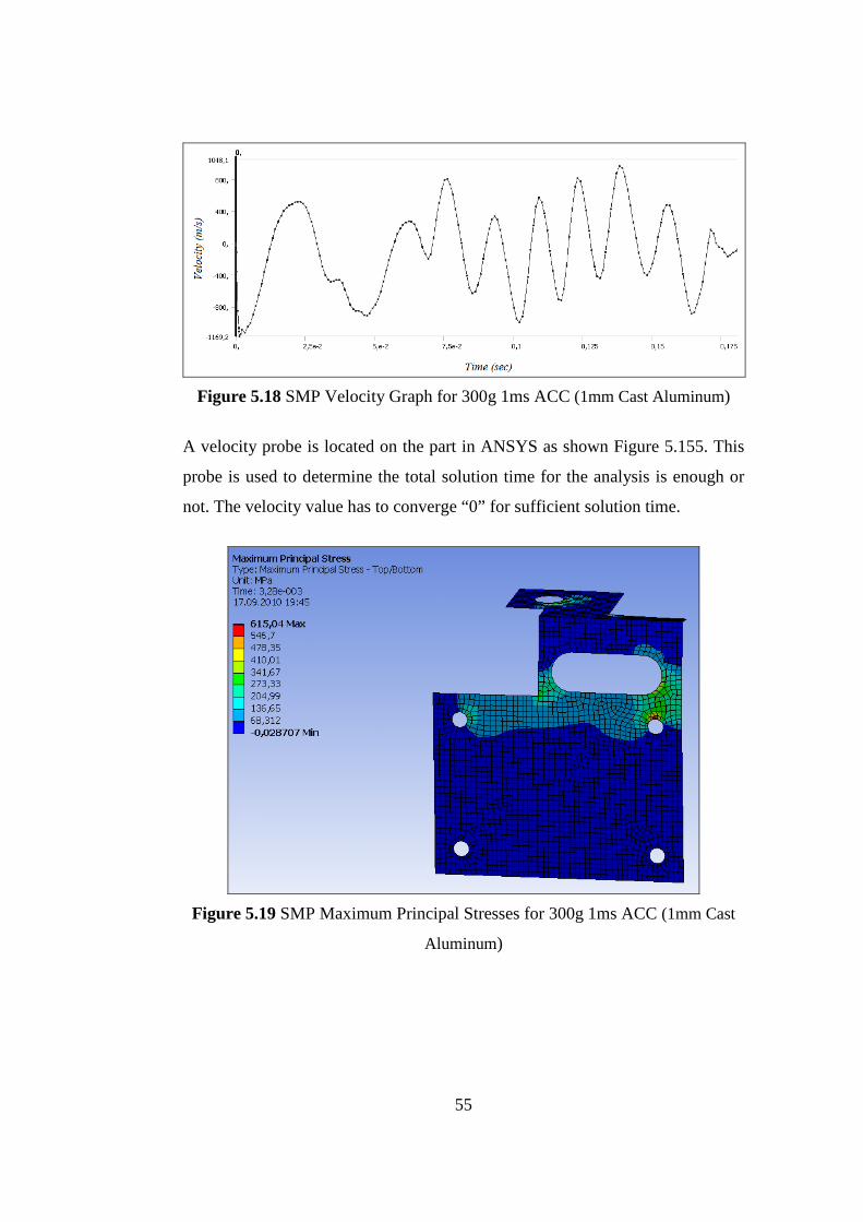
55
Figure 5.18 SMP Velocity Graph for 300g 1ms ACC (1mm Cast Aluminum)
A velocity probe is located on the part in ANSYS as shown Figure 5.155. This
probe is used to determine the total solution time for the analysis is enough or
not. The velocity value has to converge “0” for sufficient solution time.
Figure 5.19 SMP Maximum Principal Stresses for 300g 1ms ACC (1mm Cast
Aluminum)
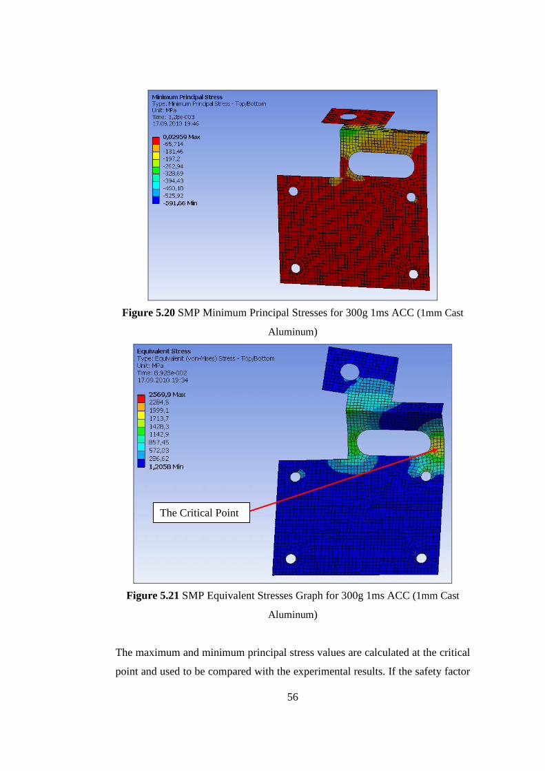
56
Figure 5.20 SMP Minimum Principal Stresses for 300g 1ms ACC (1mm Cast
Aluminum)
Figure 5.21 SMP Equivalent Stresses Graph for 300g 1ms ACC (1mm Cast
Aluminum)
The maximum and minimum principal stress values are calculated at the critical
point and used to be compared with the experimental results. If the safety factor
The Critical Point
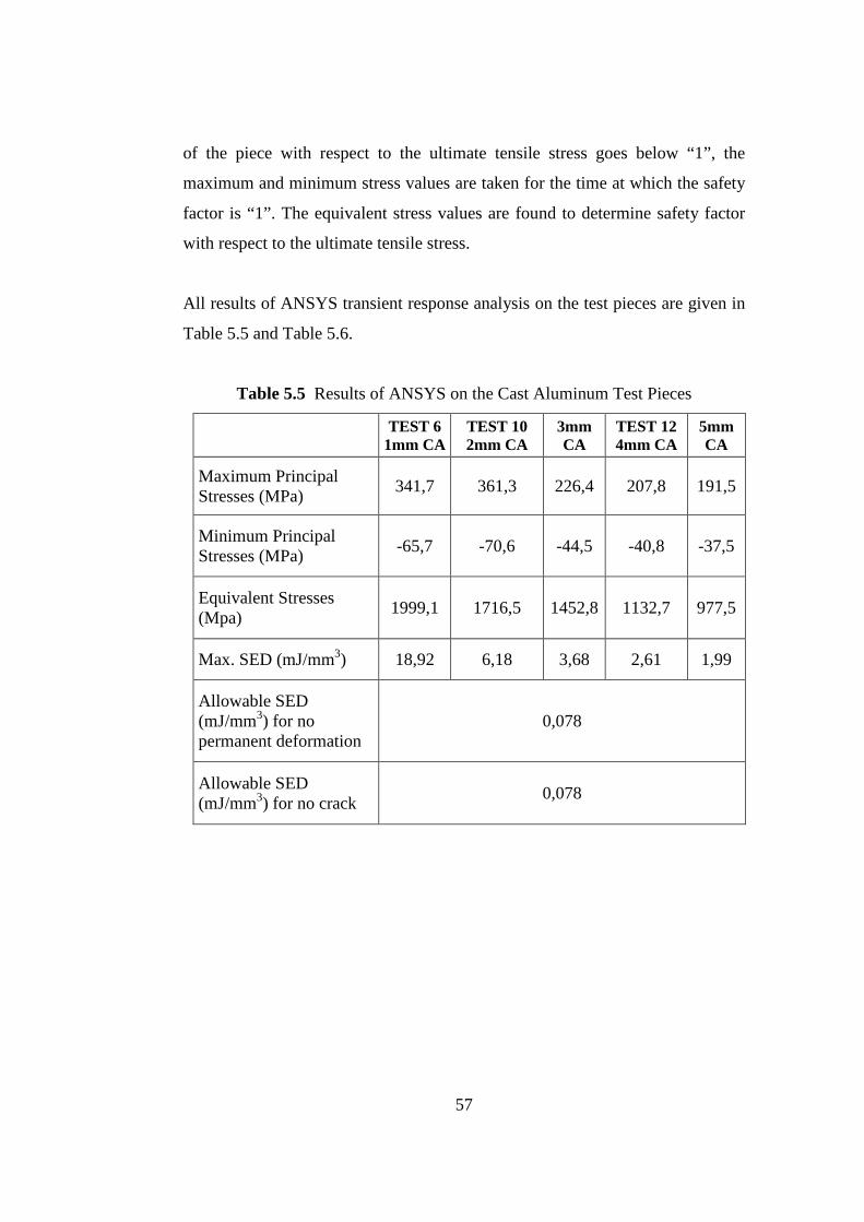
57
of the piece with respect to the ultimate tensile stress goes below “1”, the
maximum and minimum stress values are taken for the time at which the safety
factor is “1”. The equivalent stress values are found to determine safety factor
with respect to the ultimate tensile stress.
All results of ANSYS transient response analysis on the test pieces are given in
Table 5.5 and Table 5.6.
Table 5.5 Results of ANSYS on the Cast Aluminum Test Pieces
TEST 6
1mm CA TEST 10 2mm CA
3mm CA
TEST 12 4mm CA
5mm CA
Maximum Principal Stresses (MPa)
341,7 361,3 226,4 207,8 191,5
Minimum Principal Stresses (MPa)
-65,7 -70,6 -44,5 -40,8 -37,5
Equivalent Stresses (Mpa)
1999,1 1716,5 1452,8 1132,7 977,5
Max. SED (mJ/mm3) 18,92 6,18 3,68 2,61 1,99
Allowable SED (mJ/mm3) for no permanent deformation
0,078
Allowable SED (mJ/mm3) for no crack
0,078
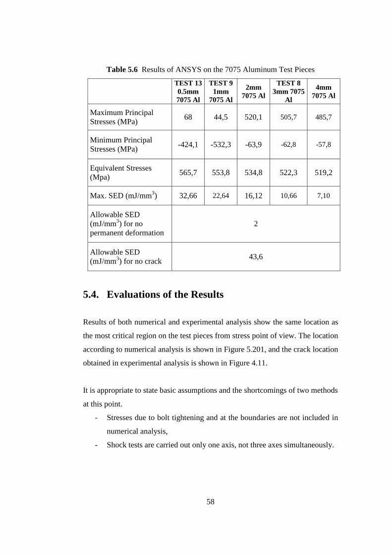
58
Table 5.6 Results of ANSYS on the 7075 Aluminum Test Pieces
TEST 13 0.5mm 7075 Al
TEST 9 1mm
7075 Al
2mm 7075 Al
TEST 8 3mm 7075
Al
4mm 7075 Al
Maximum Principal Stresses (MPa)
68 44,5 520,1 505,7 485,7
Minimum Principal Stresses (MPa)
-424,1 -532,3 -63,9 -62,8 -57,8
Equivalent Stresses (Mpa)
565,7 553,8 534,8 522,3 519,2
Max. SED (mJ/mm3) 32,66 22,64 16,12 10,66 7,10
Allowable SED (mJ/mm3) for no permanent deformation
2
Allowable SED (mJ/mm3) for no crack
43,6
5.4. Evaluations of the Results
Results of both numerical and experimental analysis show the same location as
the most critical region on the test pieces from stress point of view. The location
according to numerical analysis is shown in Figure 5.201, and the crack location
obtained in experimental analysis is shown in Figure 4.11.
It is appropriate to state basic assumptions and the shortcomings of two methods
at this point.
- Stresses due to bolt tightening and at the boundaries are not included in
numerical analysis,
- Shock tests are carried out only one axis, not three axes simultaneously.

59
Although the stress values obtained by numerical analysis are still questionable,
critical location was determined correctly. From Figure 5.222 to Figure 5.2929
all analysis results are shown graphically.
Figure 5.22 Effect of Material Thickness on Maximum SED (Cast Aluminum)
Figure 5.23 Effect of Material Thickness on Maximum SED (7075 Al)
It is seen from the graphs that the maximum strain energy density of the part is
decreasing with the increasing thickness of the material for both brittle and
ductile materials.
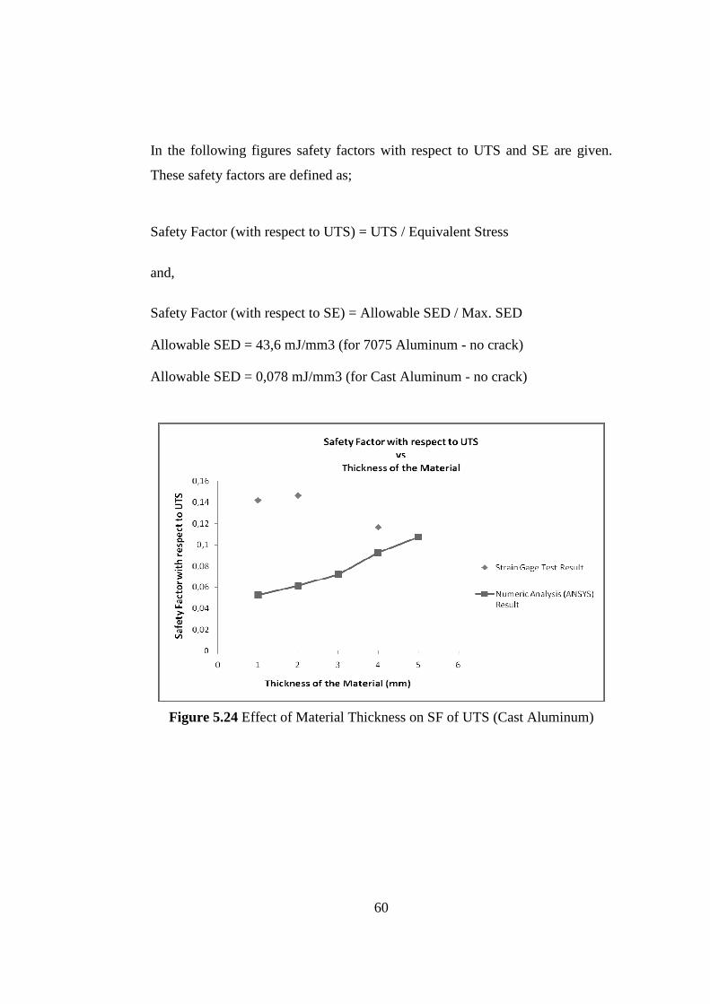
60
In the following figures safety factors with respect to UTS and SE are given.
These safety factors are defined as;
Safety Factor (with respect to UTS) = UTS / Equivalent Stress
and,
Safety Factor (with respect to SE) = Allowable SED / Max. SED
Allowable SED = 43,6 mJ/mm3 (for 7075 Aluminum - no crack)
Allowable SED = 0,078 mJ/mm3 (for Cast Aluminum - no crack)
Figure 5.24 Effect of Material Thickness on SF of UTS (Cast Aluminum)
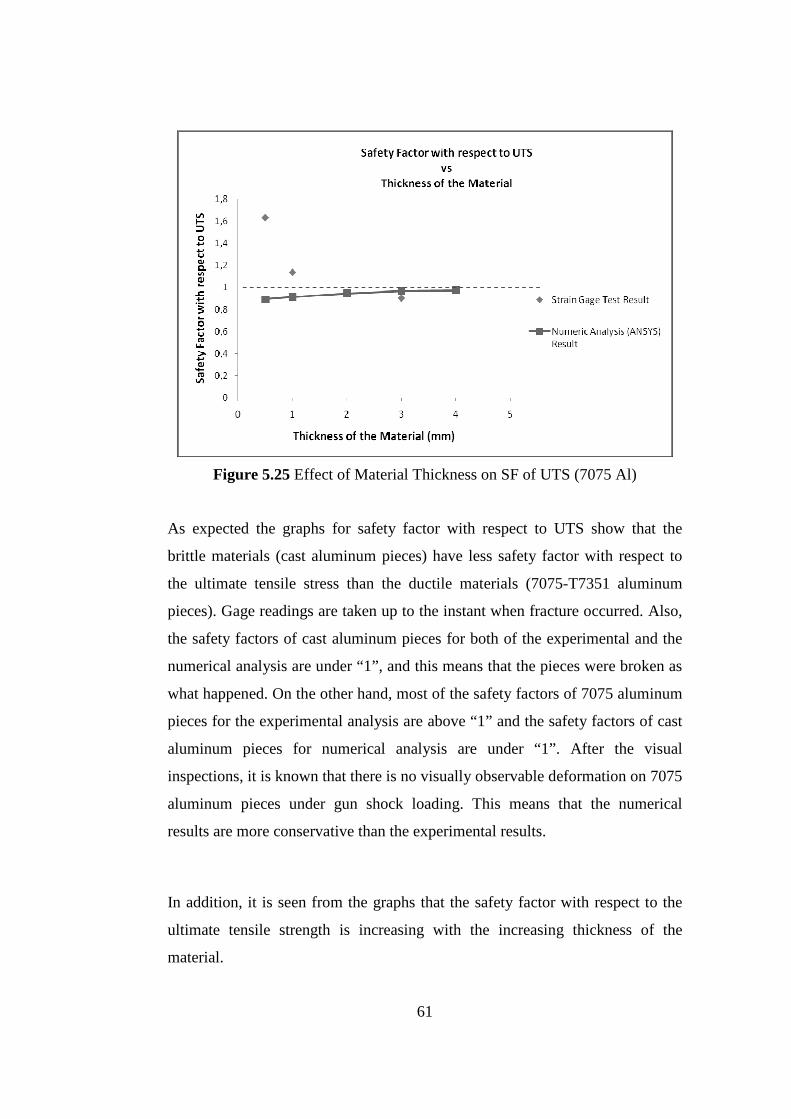
61
Figure 5.25 Effect of Material Thickness on SF of UTS (7075 Al)
As expected the graphs for safety factor with respect to UTS show that the
brittle materials (cast aluminum pieces) have less safety factor with respect to
the ultimate tensile stress than the ductile materials (7075-T7351 aluminum
pieces). Gage readings are taken up to the instant when fracture occurred. Also,
the safety factors of cast aluminum pieces for both of the experimental and the
numerical analysis are under “1”, and this means that the pieces were broken as
what happened. On the other hand, most of the safety factors of 7075 aluminum
pieces for the experimental analysis are above “1” and the safety factors of cast
aluminum pieces for numerical analysis are under “1”. After the visual
inspections, it is known that there is no visually observable deformation on 7075
aluminum pieces under gun shock loading. This means that the numerical
results are more conservative than the experimental results.
In addition, it is seen from the graphs that the safety factor with respect to the
ultimate tensile strength is increasing with the increasing thickness of the
material.
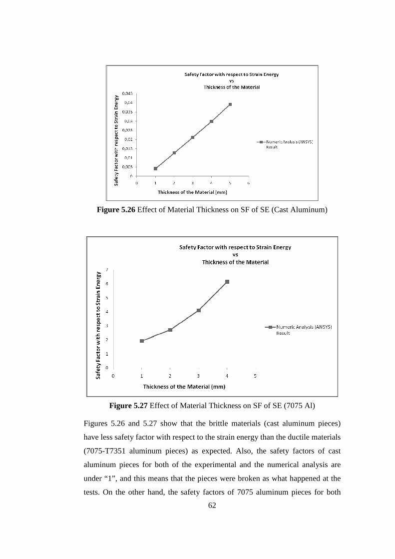
62
Figure 5.26 Effect of Material Thickness on SF of SE (Cast Aluminum)
Figure 5.27 Effect of Material Thickness on SF of SE (7075 Al)
Figures 5.26 and 5.27 show that the brittle materials (cast aluminum pieces)
have less safety factor with respect to the strain energy than the ductile materials
(7075-T7351 aluminum pieces) as expected. Also, the safety factors of cast
aluminum pieces for both of the experimental and the numerical analysis are
under “1”, and this means that the pieces were broken as what happened at the
tests. On the other hand, the safety factors of 7075 aluminum pieces for both
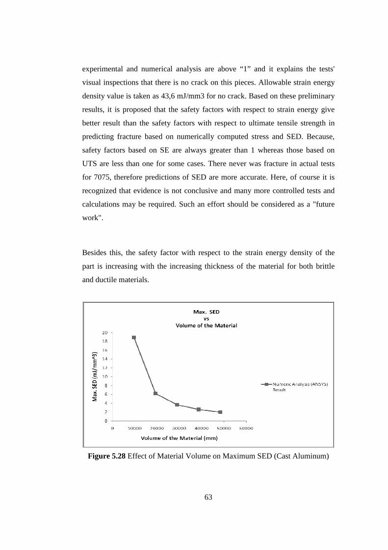
63
experimental and numerical analysis are above “1” and it explains the tests'
visual inspections that there is no crack on this pieces. Allowable strain energy
density value is taken as 43,6 mJ/mm3 for no crack. Based on these preliminary
results, it is proposed that the safety factors with respect to strain energy give
better result than the safety factors with respect to ultimate tensile strength in
predicting fracture based on numerically computed stress and SED. Because,
safety factors based on SE are always greater than 1 whereas those based on
UTS are less than one for some cases. There never was fracture in actual tests
for 7075, therefore predictions of SED are more accurate. Here, of course it is
recognized that evidence is not conclusive and many more controlled tests and
calculations may be required. Such an effort should be considered as a "future
work".
Besides this, the safety factor with respect to the strain energy density of the
part is increasing with the increasing thickness of the material for both brittle
and ductile materials.
Figure 5.28 Effect of Material Volume on Maximum SED (Cast Aluminum)
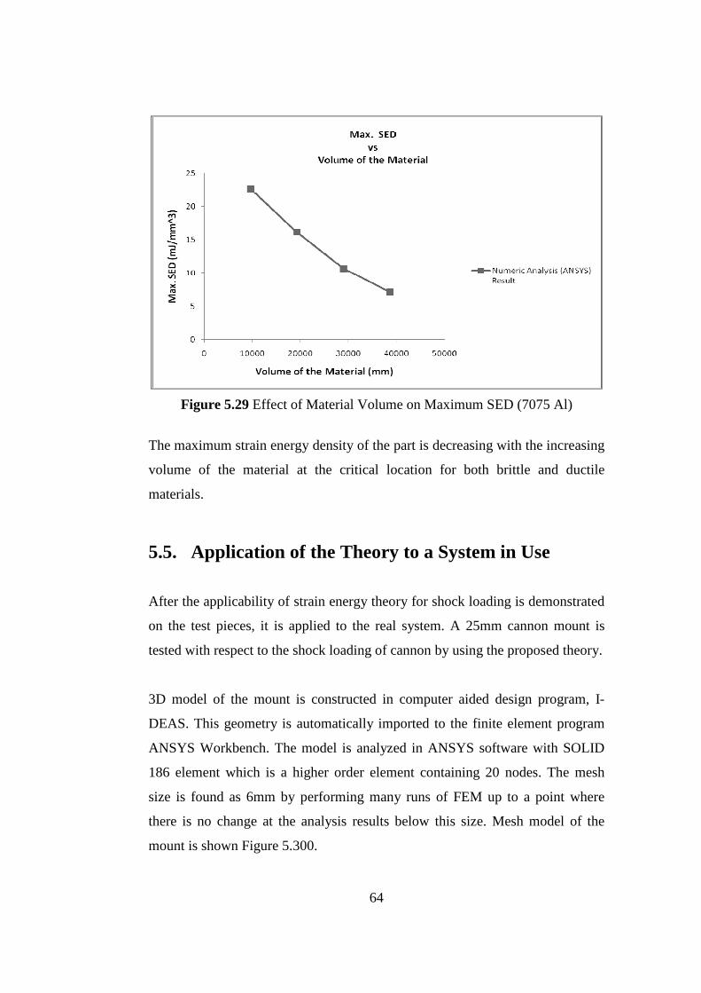
64
Figure 5.29 Effect of Material Volume on Maximum SED (7075 Al)
The maximum strain energy density of the part is decreasing with the increasing
volume of the material at the critical location for both brittle and ductile
materials.
5.5. Application of the Theory to a System in Use
After the applicability of strain energy theory for shock loading is demonstrated
on the test pieces, it is applied to the real system. A 25mm cannon mount is
tested with respect to the shock loading of cannon by using the proposed theory.
3D model of the mount is constructed in computer aided design program, I-
DEAS. This geometry is automatically imported to the finite element program
ANSYS Workbench. The model is analyzed in ANSYS software with SOLID
186 element which is a higher order element containing 20 nodes. The mesh
size is found as 6mm by performing many runs of FEM up to a point where
there is no change at the analysis results below this size. Mesh model of the
mount is shown Figure 5.300.

65
Figure 5.30 Mesh Model of the Mount
25mm cannon mount model has 9236 SOLID elements and 36359 nodes.
25mm cannon mount is made of impax steel. The material properties of impax
steel are found by literature survey and entered the material library of ANSYS
Workbench seen in Table 5.7 to Table 5.9 and Figure 5.311.
Table 5.7 Material Properties of Impax Steel [41]
Impax Steel
Elastic Region Engineering Strain (εeng_e) 0,00375
Elastic Region Engineering Stress (σeng_e) (MPa) 800
Plastic Region Engineering Strain (εeng_p) 0,175
Plastic Region Engineering Stress (σeng_p) (MPa) 930
Density (kg/mm3) 7,8 x 10⁻⁶
for elastic region of impax steel,
εtrue_e = 1n (1 + 0,00375) = 0.003743
σtrue_e = 800(1 + 0,00375) = 803 MPa
for plastic region of impax steel,
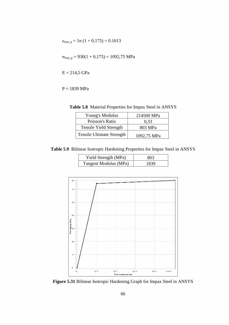
66
εtrue_p = 1n (1 + 0,175) = 0.1613
σtrue_p = 930(1 + 0,175) = 1092,75 MPa
E = 214,5 GPa
P = 1839 MPa
Table 5.8 Material Properties for Impax Steel in ANSYS
Young's Modulus 214500 MPa Poisson's Ratio 0,33
Tensile Yield Strength 803 MPa
Tensile Ultimate Strength 1092,75 MPa
Table 5.9 Bilinear Isotropic Hardening Properties for Impax Steel in ANSYS
Yield Strength (MPa) 803 Tangent Modulus (MPa) 1839
Figure 5.31 Bilinear Isotropic Hardening Graph for Impax Steel in ANSYS

67
The cannon is connected as a mass element to the mount by rigid regions at the
pin holes of the mount and boundary hole have fixed boundary condition in all
directions. These are applied on the finite element model as shown Figure
5.322.
Figure 5.32 ANSYS Model of the Mount
100 g 2ms half sine classical shock form is found appropriate for 25mm cannon
firing tests on the mount. One of the original data and SRS graph of it is shown
in Figure 5.333 and Figure 5.344.
Connection holes of the mass element
Mass element Boundary holes
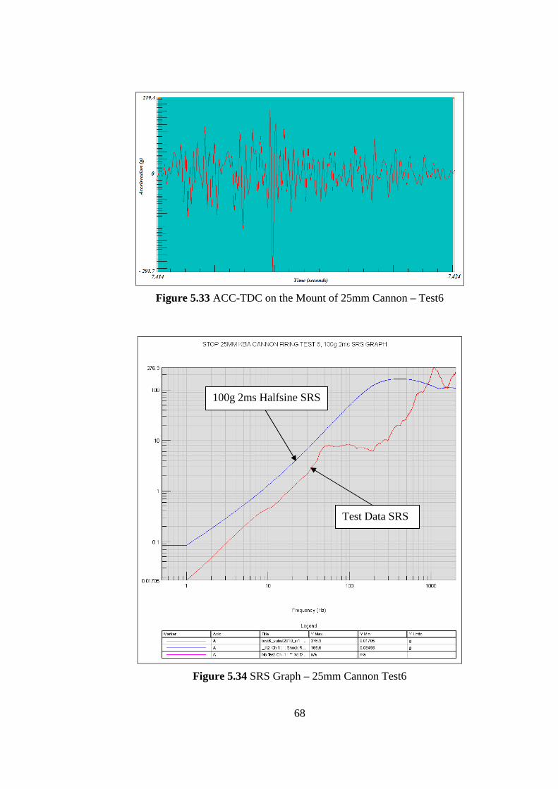
68
Figure 5.33 ACC-TDC on the Mount of 25mm Cannon – Test6
Figure 5.34 SRS Graph – 25mm Cannon Test6
Test Data SRS
100g 2ms Halfsine SRS
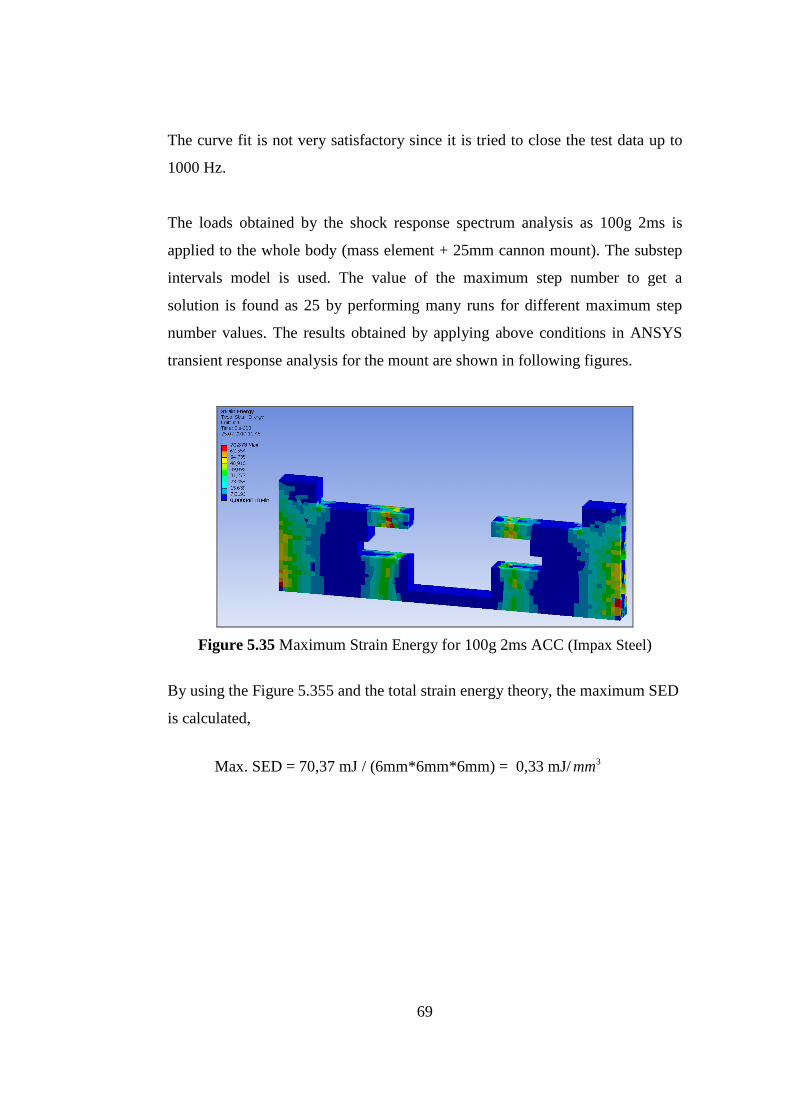
69
The curve fit is not very satisfactory since it is tried to close the test data up to
1000 Hz.
The loads obtained by the shock response spectrum analysis as 100g 2ms is
applied to the whole body (mass element + 25mm cannon mount). The substep
intervals model is used. The value of the maximum step number to get a
solution is found as 25 by performing many runs for different maximum step
number values. The results obtained by applying above conditions in ANSYS
transient response analysis for the mount are shown in following figures.
Figure 5.35 Maximum Strain Energy for 100g 2ms ACC (Impax Steel)
By using the Figure 5.355 and the total strain energy theory, the maximum SED
is calculated,
Max. SED = 70,37 mJ / (6mm*6mm*6mm) = 0,33 mJ/3mm
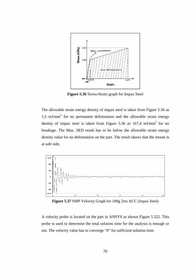
70
Figure 5.36 Stress-Strain graph for Impax Steel
The allowable strain energy density of impax steel is taken from Figure 5.36 as
1,5 mJ/mm3 for no permanent deformation and the allowable strain energy
density of impax steel is taken from Figure 5.36 as 167,4 mJ/mm3 for no
breakage. The Max. SED result has to be below the allowable strain energy
density value for no deformation on the part. The result shows that the mount is
at safe side.
Figure 5.37 SMP Velocity Graph for 100g 2ms ACC (Impax Steel)
A velocity probe is located on the part in ANSYS as shown Figure 5.322. This
probe is used to determine the total solution time for the analysis is enough or
not. The velocity value has to converge “0” for sufficient solution time.

71
Figure 5.38 SMP Maximum Principal Stresses for 100g 2ms ACC (Impax Steel)
Figure 5.39 SMP Minimum Principal Stresses for 100g 2ms ACC (Impax Steel)
All results of ANSYS transient response analysis on the mount are given in
Table 5.10.
Table 5.10 Results of ANSYS Transient Response on the 25mm Cannon Mount
25mm Cannon Mount ANSYS
Transient Analysis Results Maximum Principal Stresses (MPa) 437 Minimum Principal Stresses (MPa) -473 Max. SED (mJ/mm^3) 0.33 Allowable SED (mJ/mm^3) for no permanent deformation
1,5
Allowable SED (mJ/mm^3) for no crack
167,4
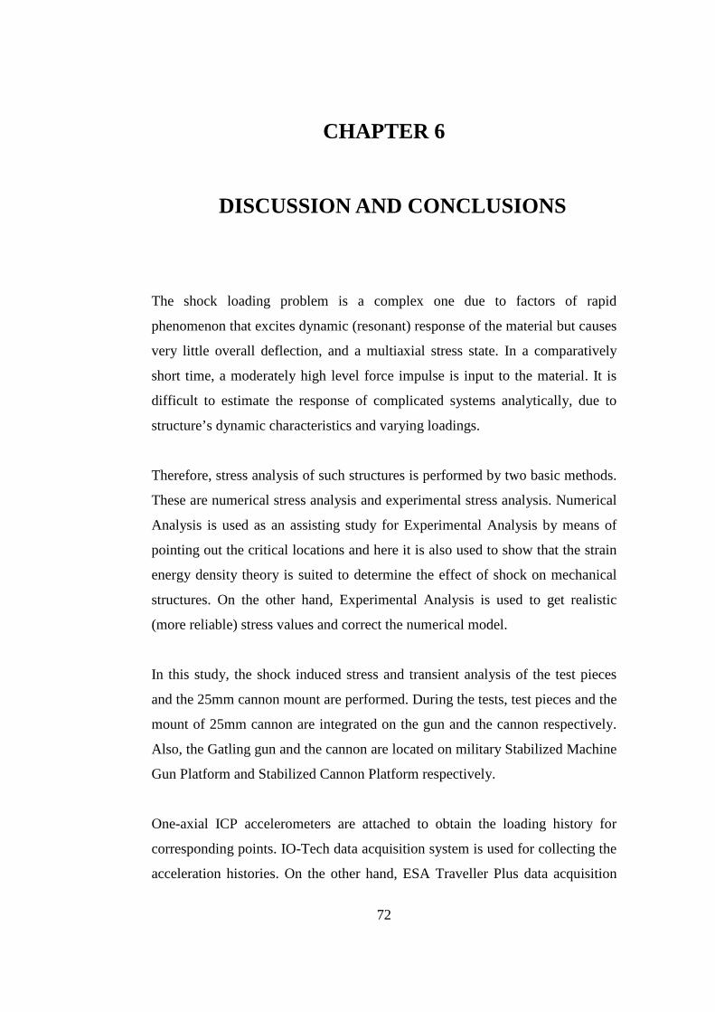
72
CHAPTER 6
6. DISCUSSION AND CONCLUSIONS
The shock loading problem is a complex one due to factors of rapid
phenomenon that excites dynamic (resonant) response of the material but causes
very little overall deflection, and a multiaxial stress state. In a comparatively
short time, a moderately high level force impulse is input to the material. It is
difficult to estimate the response of complicated systems analytically, due to
structure’s dynamic characteristics and varying loadings.
Therefore, stress analysis of such structures is performed by two basic methods.
These are numerical stress analysis and experimental stress analysis. Numerical
Analysis is used as an assisting study for Experimental Analysis by means of
pointing out the critical locations and here it is also used to show that the strain
energy density theory is suited to determine the effect of shock on mechanical
structures. On the other hand, Experimental Analysis is used to get realistic
(more reliable) stress values and correct the numerical model.
In this study, the shock induced stress and transient analysis of the test pieces
and the 25mm cannon mount are performed. During the tests, test pieces and the
mount of 25mm cannon are integrated on the gun and the cannon respectively.
Also, the Gatling gun and the cannon are located on military Stabilized Machine
Gun Platform and Stabilized Cannon Platform respectively.
One-axial ICP accelerometers are attached to obtain the loading history for
corresponding points. IO-Tech data acquisition system is used for collecting the
acceleration histories. On the other hand, ESA Traveller Plus data acquisition
73
system is used for collecting the strain histories. Initially, the test pieces were
equipped with a rectangular rosette to obtain stress histories of specific locations
which is required to perform strain analysis of the structures. They were settled
next to the slot of the parts, since that portion was under consideration as a
strain region in this study. In addition, detailed visual inspections are done on
the parts and failures are observed during and after the test.
Furthermore, experimental stress analysis due to shock loading is performed for
two different types of material of the test pieces and different thicknesses of the
test pieces. The input data for the analysis is obtained through measurements
from strain rosette precisely located at the critical location of the test pieces.
ESAM is used for performing the experimental stress analysis and rosette
calculations. Maximum principal stress, minimum principal stress, principal
stress direction, absolute principal stress and Von Misses stress are the results of
the analysis. Among them, maximum principal stress and minimum principal
stress are the main parameters of interest as an output and they are used for
comparison with numerical results.
Shock Response Spectrum (SRS) analysis is done by using nCode Glypworks to
define the equivalent shock profiles created on test pieces and the mount of
25mm cannon by means of the gun and the cannon firing. In FEM, it is not
possible to apply the original acceleration time history as a load since the
solution of this problem takes too much time. Hence we try to obtain a classical
shock form which supplies approximately the same effects of the original data
as a load in FEM. Different types, amplitudes and times values of classical
forms are tried to get the best fitted curve. Classical shock forms are 300 g 1ms
half sine for 12.7mm Gatling gun firing tests on the test pieces and 100 g 2ms
half sine 25mm cannon firing tests on the mount.
Transient shock analysis of the test pieces are done by applying the obtained
shock profiles on the part in a finite element model (ANSYS) to find the
74
numerical stress values. FEM analysis is performed in terms of elasto-plastic
behavior due to shock loading. The material properties of 7075-T7351
aluminum are found by literature survey. On the other hand, material properties
of cast aluminum are found by tensile test. In ANSYS, all stress-strain inputs
are converted true stress and true (or logarithmic) strain and results in all
outputs are given also as true stress and true strain. In addition, bilinear isotropic
hardening plasticity material model is used in large strain analyses in ANSYS.
300g 1ms obtained by the shock response spectrum analysis is applied to the
whole body.
Numerical and experimental stress values are compared to verify the finite
element models (FEM). Both of the numerical and the experimental analysis
show the same location as the most critical region on the test pieces from stress
point of view.
Finally, the stress and strain energy density values are used to define safety
factors. An attempt is made to discover which safety factors give more accurate
results concerning failure under the effect of shock loading on the parts.
The followings are also concluded from the analysis;
- The maximum strain energy density of the part is decreasing with the
increasing thickness of the material for both brittle (cast aluminum
pieces) and ductile materials (7075-T7351 aluminum pieces).
- The numerical results are more conservative than the experimental
results.
75
- The safety factors with respect to strain energy give better result than the
safety factors with respect to ultimate tensile strength in predicting
failure by fracture.
- The safety factor with respect to the strain energy density of the part is
increasing with the increasing thickness of the material for both brittle
and ductile materials.
- The maximum strain energy density of the part is decreasing with the
increasing volume of the material for both brittle and ductile materials. It
is showed that the materials resist to shock loading with their volumes.
After demonstrating the use of strain energy density theory on the test pieces for
determining the shock failure at military structures, it is applied to the real
system. 25mm cannon mount is tested with respect to the shock loading of
cannon by using the theory. 100g 2ms obtained by the shock response spectrum
analysis is applied to the whole body and as a result the mount is found on the
safe side as expected.
As a future work, force response spectrum analysis (FRS) can be applied instead
of SRS while performing the numerical analysis of the gun firing shock in the
finite element model. In the NATO paper [24], it is proposed that FRS analysis
is better way in order supply equivalent force input.
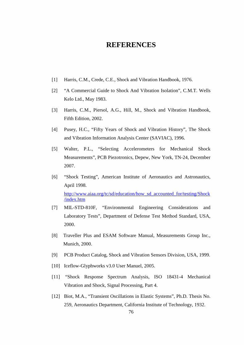
76
REFERENCES
[1] Harris, C.M., Crede, C.E., Shock and Vibration Handbook, 1976.
[2] “A Commercial Guide to Shock And Vibration Isolation”, C.M.T. Wells
Kelo Ltd., May 1983.
[3] Harris, C.M., Piersol, A.G., Hill, M., Shock and Vibration Handbook,
Fifth Edition, 2002.
[4] Pusey, H.C., “Fifty Years of Shock and Vibration History”, The Shock
and Vibration Information Analysis Center (SAVIAC), 1996.
[5] Walter, P.L., “Selecting Accelerometers for Mechanical Shock
Measurements”, PCB Piezotronics, Depew, New York, TN-24, December
2007.
[6] “Shock Testing”, American Institute of Aeronautics and Astronautics,
April 1998.
http://www.aiaa.org/tc/sd/education/how_sd_accounted_for/testing/Shock/index.htm
[7] MIL-STD-810F, “Environmental Engineering Considerations and
Laboratory Tests”, Department of Defense Test Method Standard, USA,
2000.
[8] Traveller Plus and ESAM Software Manual, Measurements Group Inc.,
Munich, 2000.
[9] PCB Product Catalog, Shock and Vibration Sensors Division, USA, 1999.
[10] Iceflow-Glyphworks v3.0 User Manuel, 2005.
[11] “Shock Response Spectrum Analysis, ISO 18431-4 Mechanical
Vibration and Shock, Signal Processing, Part 4.
[12] Biot, M.A., “Transient Oscillations in Elastic Systems”, Ph.D. Thesis No.
259, Aeronautics Department, California Institute of Technology, 1932.
77
[13] Housner, G.W., “Behavior of Structures During Earthquakes,” J. of Eng.
Mech. Div., ASCE, Vol. 85, No. EM4, pp. 109-129, 1959.
[14] Newmark, N.M., “A Method of Computation for Structural Dynamics”,
ASCE Journal of the Engineering Mechanics Division, Vol. 85 No. EM3,
1959.
[15] Newmark, N.M., Rosenblueth, “Fundamentals of Earthquake
Engineering”, Prentice-Hall, 1971.
[16] Kelly, R.D., Richman, G., “Principles and Techniques of Shock Data
Analysis”, The Shock and Vibration Information Center, Washington,
D.C., 1969.
[17] Martin, J.N., Sinclair, A.J., Foster, W.A., “On the Shock Response
Spectrum Recursive Algorithm of Kelly and Richman”, Aerospace
Engineering Department, Auburn University, Auburn, NASA Technical
Reports, 2010.
[18] Walter, P.L., “Selecting Accelerometers for Mechanical Shock
Measurements”, PCB Piezotronics, Depew, New York and Texas
Christian University, Sound and Vibration, Fort Worth, Texas, pp. 14-18,
December 2007.
[19] Alexander, J.E., “Shock Response Spectrum – A Primer”, BAE Systems,
US Combat Systems Minneapolis, Minneapolis, Minnesota, Sound and
Vibration, pp. 6-14, June 2009.
[20] Smith, S., Roy, M., “Why Shock Measurements Performed at Different
Facilities Don’t Agree”, Proceedings of the 66th Shock and Vibration
Symposium, Biloxi, MS Thesis, 1995.
[21] Hollowell, B., Smith, S., “Proposed Method to Standardize Shock
Response Spectrum (SRS) Analysis (To Provide Agreement Between
Tests Performed at Different Facilities)”, IES Journal, May/June 1996.
[22] TUMA, J., Koci, P., “Calculation of Shock Response Spectrum”,
Colloquium Dynamics of Machines 2009, Prague, February 2009.

78
[23] Çelik, M., “Kaideye Monteli Stinger Sisteminin Taret Deneysel Yorulma
Analizi” SAVTEK-2002 Savunma Teknolojileri Kongresi, Orta Doğu
Teknik Üniversitesi, Ankara, pp. 321-332, 2002.
[24] Çelik, M., “Gunfire Vibration of a Stabilized Machine Gun Platform”,
RTO-MP-AVT-152 NATO-RTO Symposium on Limit Cycle Oscillation
and Other Amplitude-Limited Self-Excited Vibrations, Loen, Norway.
[25] Petrusa, D.C., “Evaluation and Analysis of DDG-81 Simulated
Athwartship Shock Response”, Naval Postgraduate School Monterey,
California, MS Thesis, June 2004.
[26] Parlak, M., “Bir Hava Savunma Sisteminin Deneysel Şok Analizi”, 11.
Ulusal Makina Teorisi Sempozyumu, Gazi Üniversitesi, Mühendislik-
Mimarlık Fakültesi, Ankara, Eylül 2003.
[27] Rusovici, R., “Modeling of Shock Wave Propagation and Attenuation in
Viscoelastic Structures”, PhD Thesis, Mechanical Engineering, Virginia
Polytechnic Institute and State University, September 1999.
[28] Carpinteri, A., Macha, E., Brighenti, R., Spagnoli, A., “Expected
Principal Stress Directions under Multiaxial Loading”, International
Journal of Fatigue, Vol.21, pp.83-96, 1999.
[29] Shang, G., Wang, K., Li, M., Yao, W., “Local Stress-Strain Field
Intensity Approach to Fatigue Life Prediction under Random Cyclic
Loading”, International Journal of Fatigue, Vol.23, pp.903-910, 2001.
[30] Irvine, T., “An Introduction to the Shock Response Spectrum”,
Vibrationdata, July 2010.
http://www.vibrationdata.com/tutorials2/srs_intr.pdf
[31] Sayman O., Karakuzu R., Zor M., Şen F., “Mukavemet I, II”, D.E.Ü.
Mühendislik Fakültesi Yayınları No:250.
[32] Collins, J.A., “Failure of Materials in Mechanical Design”, Wiley-
Interscience, New York, 1981.

79
[33] Gandelsman, M., “Strain Energy in Uniaxial Loads”, Engineering
Mechanics, UNL College of Engineering and Technology, 1999.
http://emweb.unl.edu/Mechanics-Pages/Marina-Gandelsman/strain.html
[34] Benham, P.P, Warnock, F.V., “Mechanics of Solids and Structures”,
Pitman Publishing, London, 1973.
[35] Newmark, N. M., “A Method of Computation for Structural Dynamics”,
ASCE Journal of the Engineering Mechanics Division, Vol. 85 No. EM3,
1959.
[36] Wilson E., “Dynamic Analysis by Numerical Integration”, Static and
Dynamic Analysis, Technical Paper, 1998.
http://www.csiberkeley.com/
[37] Catalogs for Strain Gages Accessories and Instruments, Measurements
Group-Vishay, 2005.
[38] Traveler Strain Master Manual, ESA Messtecknik Inc., Munich, 2004.
[39] ANSYS Release 8.1 User’s Manual, ANSYS Inc., USA, 2003.
[40] Chao, Y. J., Wang, Y., Miller, K. W., “Effect of Friction Stir Welding on
Dynamic Properties of AA2024-T3 and AA7075-T7351”, August 2001.
[41] “Impax® Supreme”, Prehardened mold steel catalog, 2009.
[42] MIL-STD-810G, “Environmental Engineering Considerations and
Laboratory Tests”, Department of Defense Test Method Standard, USA,
2008.
[43] Kang, S., “Friction and Elasto-Plastic Deformation in Asperity Collision”,
Lulea University of Technology, Department of Applied Physics and
Mechanical Engineering, MS Thesis, 2010.

80
APPENDIX A
A. EQUIPMENT USED THROUGHOUT TESTS
1) Iotech data acquisition system
a. Maximum Aggregate Speed : 500 kHz
b. 72 input channels.
Figure A.1 IOtech data acquisition system
2) Traveler Strain Master data acquisition system
a. Maximum Aggregate Speed : 300 kHz
b. 32 input channels.
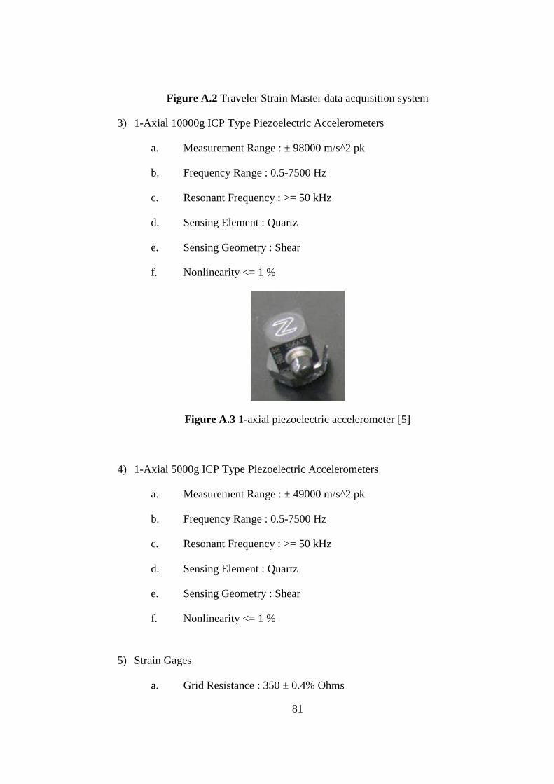
81
Figure A.2 Traveler Strain Master data acquisition system
3) 1-Axial 10000g ICP Type Piezoelectric Accelerometers
a. Measurement Range : ± 98000 m/s^2 pk
b. Frequency Range : 0.5-7500 Hz
c. Resonant Frequency : >= 50 kHz
d. Sensing Element : Quartz
e. Sensing Geometry : Shear
f. Nonlinearity <= 1 %
Figure A.3 1-axial piezoelectric accelerometer [5]
4) 1-Axial 5000g ICP Type Piezoelectric Accelerometers
a. Measurement Range : ± 49000 m/s^2 pk
b. Frequency Range : 0.5-7500 Hz
c. Resonant Frequency : >= 50 kHz
d. Sensing Element : Quartz
e. Sensing Geometry : Shear
f. Nonlinearity <= 1 %
5) Strain Gages
a. Grid Resistance : 350 ± 0.4% Ohms
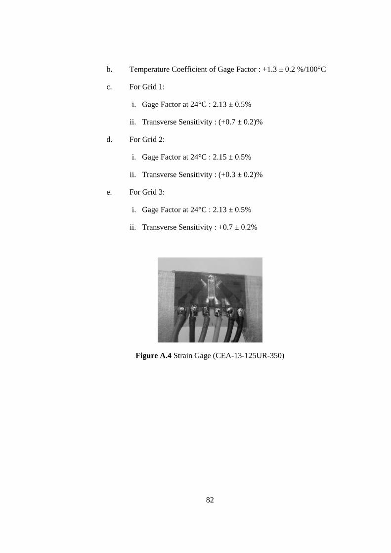
82
b. Temperature Coefficient of Gage Factor : +1.3 ± 0.2 %/100°C
c. For Grid 1:
i. Gage Factor at 24°C : 2.13 ± 0.5%
ii. Transverse Sensitivity : (+0.7 ± 0.2)%
d. For Grid 2:
i. Gage Factor at 24°C : 2.15 ± 0.5%
ii. Transverse Sensitivity : (+0.3 ± 0.2)%
e. For Grid 3:
i. Gage Factor at 24°C : 2.13 ± 0.5%
ii. Transverse Sensitivity : +0.7 ± 0.2%
Figure A.4 Strain Gage (CEA-13-125UR-350)
83
APPENDIX B
B. STRAIN ROSETTE ANALYSIS [8]
Rosettes are used for reducing strain data obtained from measurements made
with three-element or two-element strain gage rosettes.
There are three basic geometry types of strain gage rosettes:
45°- Rectangular : three grids, with the second and third grids angularly
displaced from the first grid by 45° and 90°, respectively,
60°- Delta : three grids, with the second and third grids 60° and
120°, respectively, from the first grid.
T-Rosettes : two mutually perpendicular grids.
Since three element 45°- Rectangular rosettes are used in this study, brief
formulae definitions of the kind will be covered in this section.
e e e1 2 3 : Measured strains for grids 1, 2 and 3 respectively,
ε ε ε1 2 3 : Calculated strains for grids 1, 2 and 3 respectively,
ε εmin max : Calculated maximal and minimal principal strains,
σ σmin max : Calculated maximal and minimal stresses,
K K Kt t t1 2 3, , : Transverse sensitivities of gages 1, 2 and 3,
E : Modulus of elasticity of the material,
ν : Poisson's ratio of the material,
θ : Calculated direction of principal strains.

84
B.1 Rectangular Rosette:
Correction for transverse sensitivity errors,
( ) ( )ε
ν ν1
1 31 1
11 1 3
1 3
=− − −e K K e K
K K
t t t
t t- (B.1)
( ) ( )( ) ( )( )[ ]( )( )ε
ν ν2
2
2
1 31
1
1 1 1 1
1 1
2 2 1 3 3 1
1 3 2
=−
−−
− − + − −
− −
e K
Kt
K e K K e K K
K K K
t t t t t t
t t t
(B.2)
( ) ( )εν ν
3
3 11 1
13 3 1
1 3
=− − −
−
e K K e K
K K
t t t
t t
(B.3)
Maximal principal strain,
( ) ( )εmax =+
+ − + −e e
e e e e1 21 2
2
2 3
2
2
1
2 (B.4)
Minimal principal strain,
( ) ( )εmin =+
− − + −e e
e e e e1 3
1 2
2
2 3
2
2
1
2 (B.5)
Direction (angle) from Grid 1 to the principal axis,
−−−= −
31
3121 2tan
2
1
ee
eeeθ (B.6)

85
B.2 Principal Stresses:
If the material is homogenous and isotropic, Hooke’s Law can be used with the
above equations to calculate the principal stresses, by defining elastic modulus
(E) and the Poisson’s ratio (ν ).
Maximal principal stress,
( ) 106
minmax2max 1
E −×+−
= ενεν
σ (B.7)
Minimal principal stress,
( ) 106
maxmin2min 1
E −×+−
= ενεν
σ (B.8)
In these formulas, it is assumed that maxε and minε are expressed in µm/m.
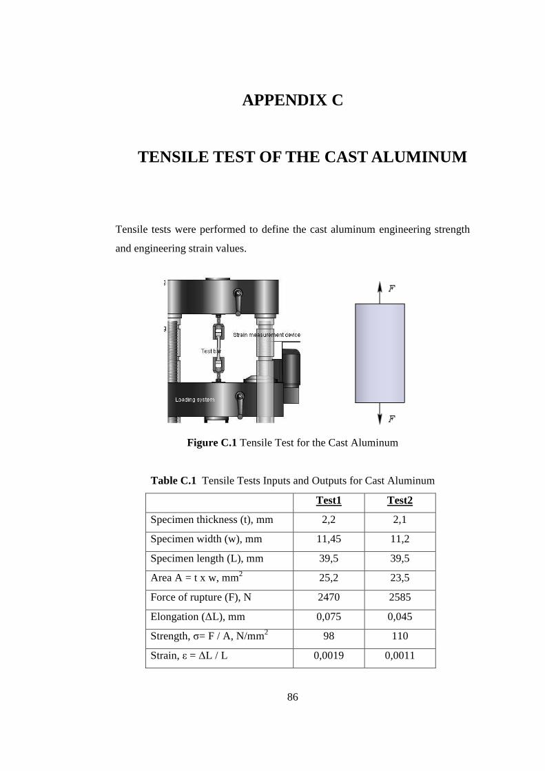
86
APPENDIX C
C. TENSILE TEST OF THE CAST ALUMINUM
Tensile tests were performed to define the cast aluminum engineering strength
and engineering strain values.
Figure C.1 Tensile Test for the Cast Aluminum
Table C.1 Tensile Tests Inputs and Outputs for Cast Aluminum
Test1 Test2
Specimen thickness (t), mm 2,2 2,1
Specimen width (w), mm 11,45 11,2
Specimen length (L), mm 39,5 39,5
Area A = t x w, mm2 25,2 23,5
Force of rupture (F), N 2470 2585
Elongation (∆L), mm 0,075 0,045
Strength, σ= F / A, N/mm2 98 110
Strain, ε = ∆L / L 0,0019 0,0011
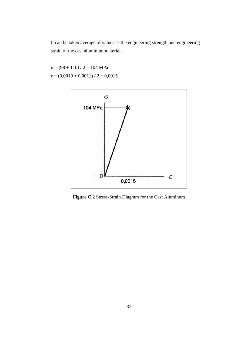
87
It can be taken average of values as the engineering strength and engineering
strain of the cast aluminum material.
σ = (98 + 110) / 2 = 104 MPa
ε = (0,0019 + 0,0011) / 2 = 0,0015
Figure C.2 Stress-Strain Diagram for the Cast Aluminum
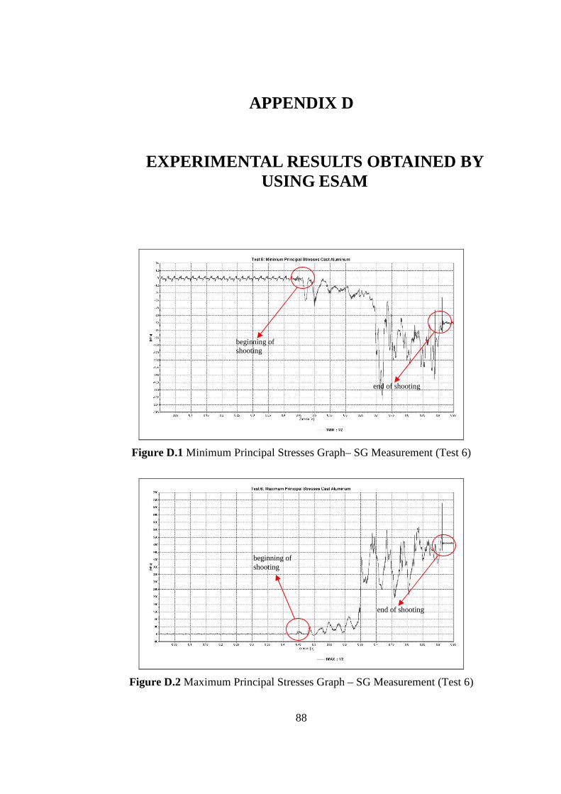
88
APPENDIX D
D. EXPERIMENTAL RESULTS OBTAINED BY USING ESAM
Figure D.1 Minimum Principal Stresses Graph– SG Measurement (Test 6)
Figure D.2 Maximum Principal Stresses Graph – SG Measurement (Test 6)
beginning of shooting
end of shooting
end of shooting
beginning of shooting

89
Figure D.3 Minimum Principal Stresses Graph – SG Measurement (Test 10)
Figure D.4 Maximum Principal Stresses Graph – SG Measurement (Test 10)
beginning of shooting
end of shooting
beginning of shooting
end of shooting
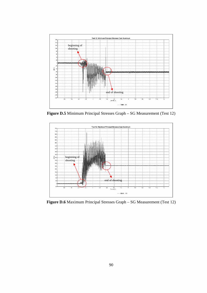
90
Figure D.5 Minimum Principal Stresses Graph – SG Measurement (Test 12)
Figure D.6 Maximum Principal Stresses Graph – SG Measurement (Test 12)
beginning of shooting
end of shooting
beginning of shooting
end of shooting

91
Figure D.7 Minimum Principal Stresses Graph – SG Measurement (Test 13)
Figure D.8 Maximum Principal Stresses Graph – SG Measurement (Test 13)
beginning of shooting
end of shooting
beginning of shooting end of shooting
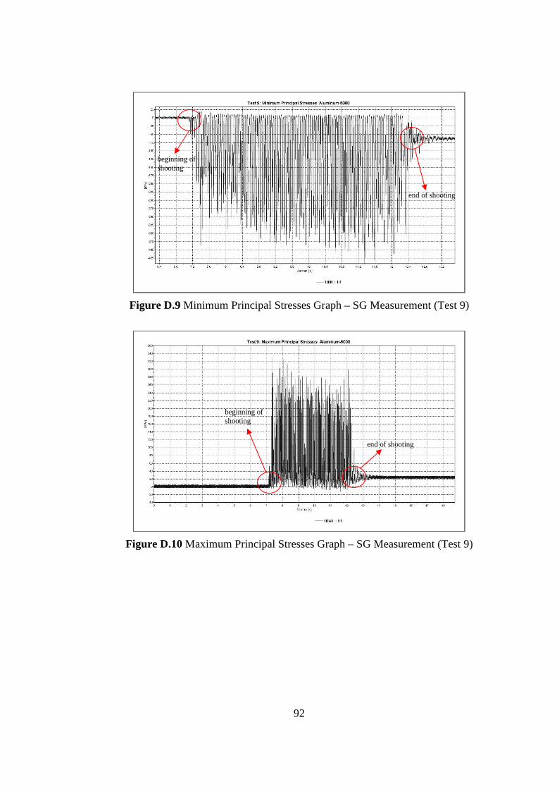
92
Figure D.9 Minimum Principal Stresses Graph – SG Measurement (Test 9)
Figure D.10 Maximum Principal Stresses Graph – SG Measurement (Test 9)
beginning of shooting
end of shooting
beginning of shooting
end of shooting
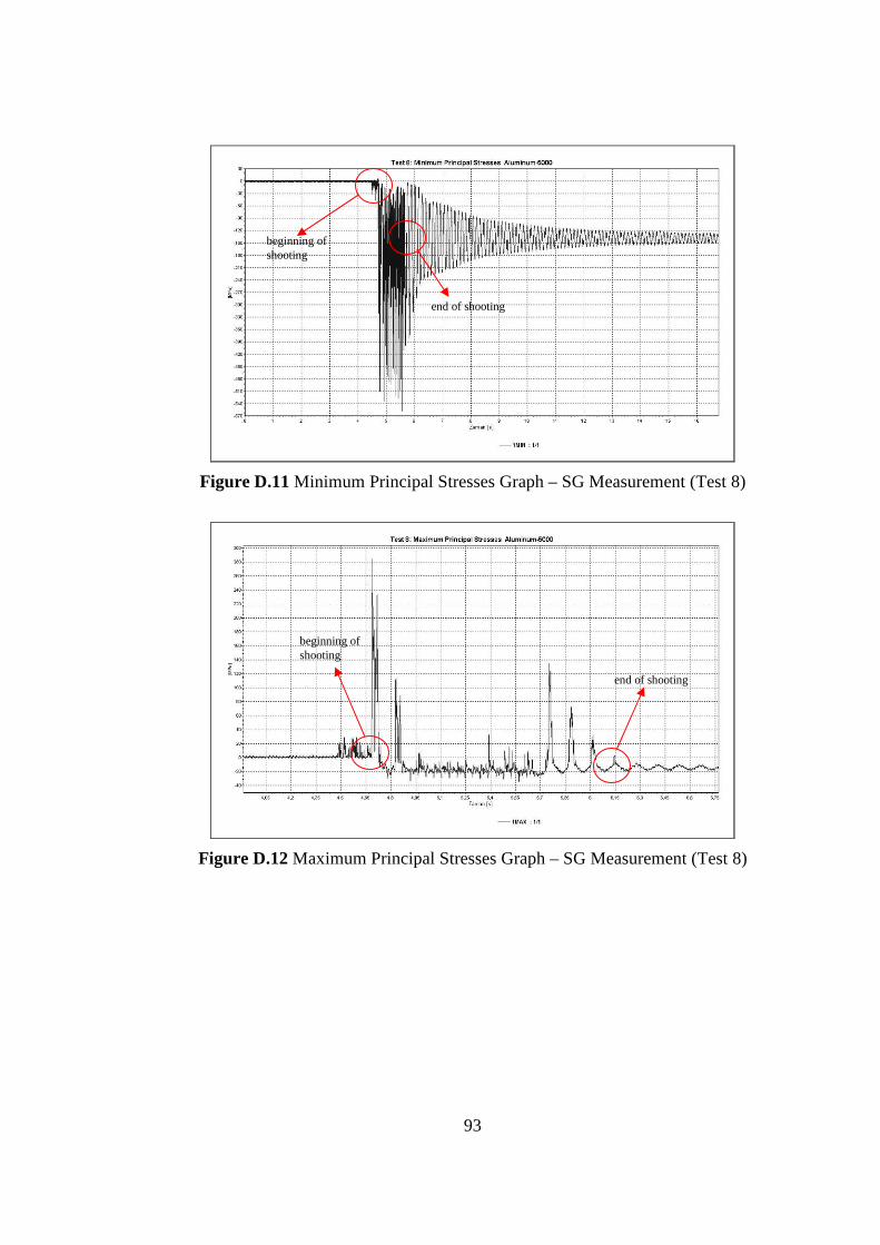
93
Figure D.11 Minimum Principal Stresses Graph – SG Measurement (Test 8)
Figure D.12 Maximum Principal Stresses Graph – SG Measurement (Test 8)
beginning of shooting
end of shooting
beginning of shooting
end of shooting
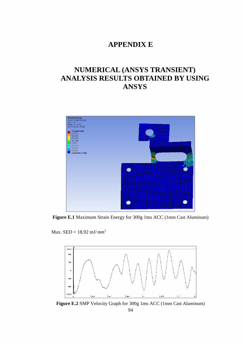
94
APPENDIX E
E. NUMERICAL (ANSYS TRANSIENT) ANALYSIS RESULTS OBTAINED BY USING
ANSYS
Figure E.1 Maximum Strain Energy for 300g 1ms ACC (1mm Cast Aluminum)
Max. SED = 18,92 mJ/ 3mm
Figure E.2 SMP Velocity Graph for 300g 1ms ACC (1mm Cast Aluminum)
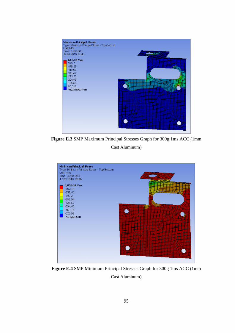
95
Figure E.3 SMP Maximum Principal Stresses Graph for 300g 1ms ACC (1mm
Cast Aluminum)
Figure E.4 SMP Minimum Principal Stresses Graph for 300g 1ms ACC (1mm
Cast Aluminum)
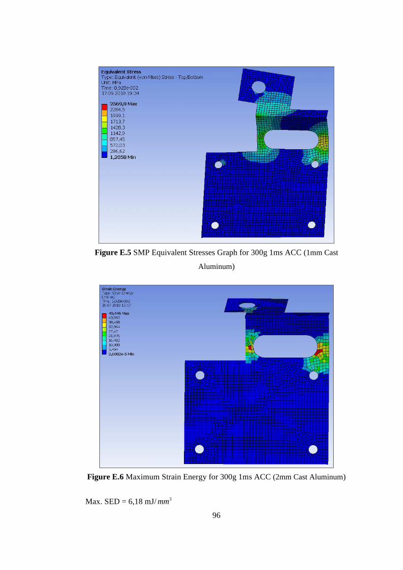
96
Figure E.5 SMP Equivalent Stresses Graph for 300g 1ms ACC (1mm Cast
Aluminum)
Figure E.6 Maximum Strain Energy for 300g 1ms ACC (2mm Cast Aluminum)
Max. SED = 6,18 mJ/ 3mm
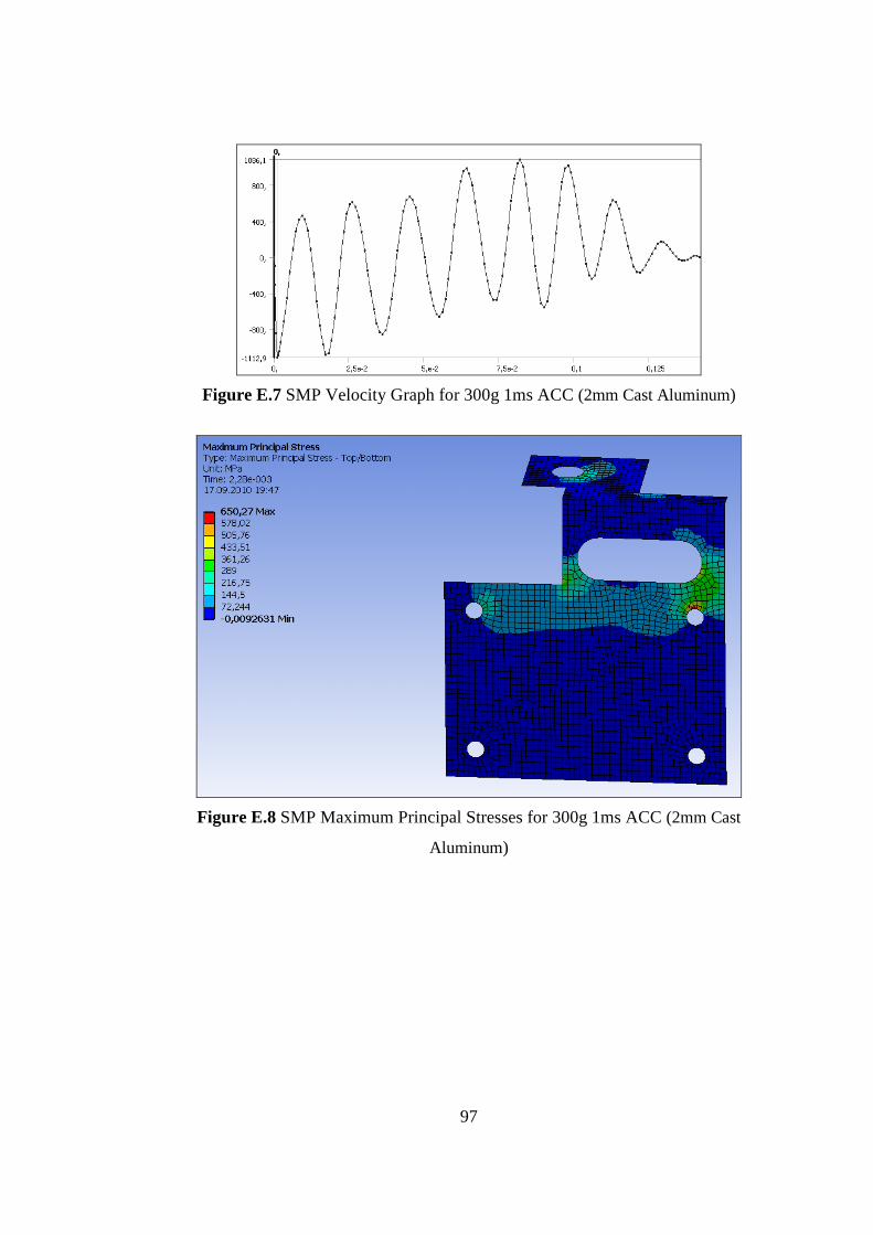
97
Figure E.7 SMP Velocity Graph for 300g 1ms ACC (2mm Cast Aluminum)
Figure E.8 SMP Maximum Principal Stresses for 300g 1ms ACC (2mm Cast
Aluminum)
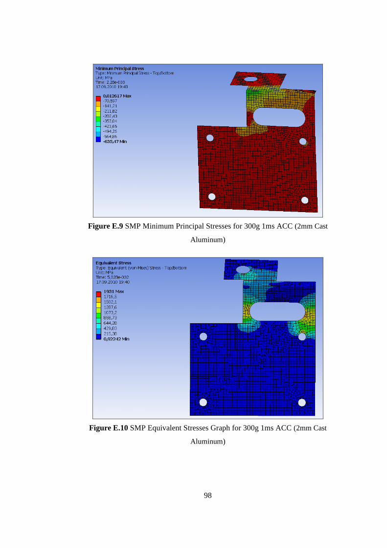
98
Figure E.9 SMP Minimum Principal Stresses for 300g 1ms ACC (2mm Cast
Aluminum)
Figure E.10 SMP Equivalent Stresses Graph for 300g 1ms ACC (2mm Cast
Aluminum)
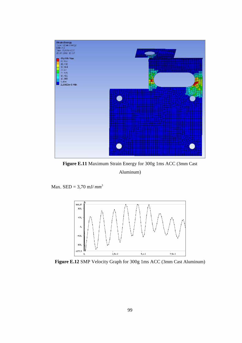
99
Figure E.11 Maximum Strain Energy for 300g 1ms ACC (3mm Cast
Aluminum)
Max. SED = 3,70 mJ/ 3mm
Figure E.12 SMP Velocity Graph for 300g 1ms ACC (3mm Cast Aluminum)
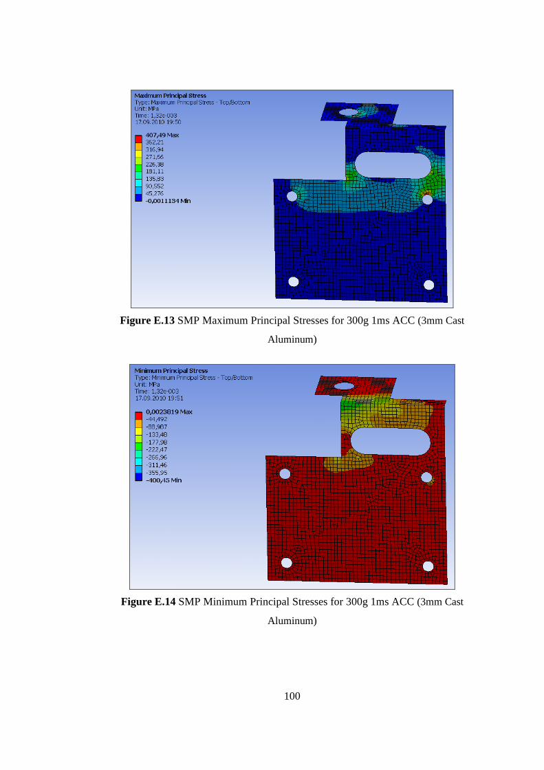
100
Figure E.13 SMP Maximum Principal Stresses for 300g 1ms ACC (3mm Cast
Aluminum)
Figure E.14 SMP Minimum Principal Stresses for 300g 1ms ACC (3mm Cast
Aluminum)

101
Figure E.15 SMP Equivalent Stresses Graph for 300g 1ms ACC (3mm Cast
Aluminum)
Figure E.16 Maximum Strain Energy for 300g 1ms ACC (4mm Cast
Aluminum)
Max. SED = 2,61 mJ/ 3mm
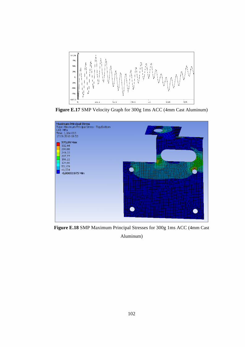
102
Figure E.17 SMP Velocity Graph for 300g 1ms ACC (4mm Cast Aluminum)
Figure E.18 SMP Maximum Principal Stresses for 300g 1ms ACC (4mm Cast
Aluminum)
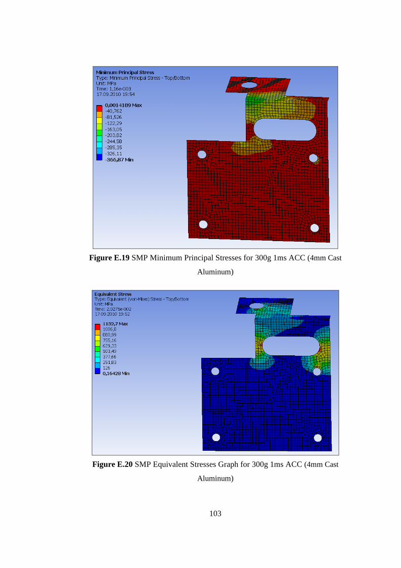
103
Figure E.19 SMP Minimum Principal Stresses for 300g 1ms ACC (4mm Cast
Aluminum)
Figure E.20 SMP Equivalent Stresses Graph for 300g 1ms ACC (4mm Cast
Aluminum)
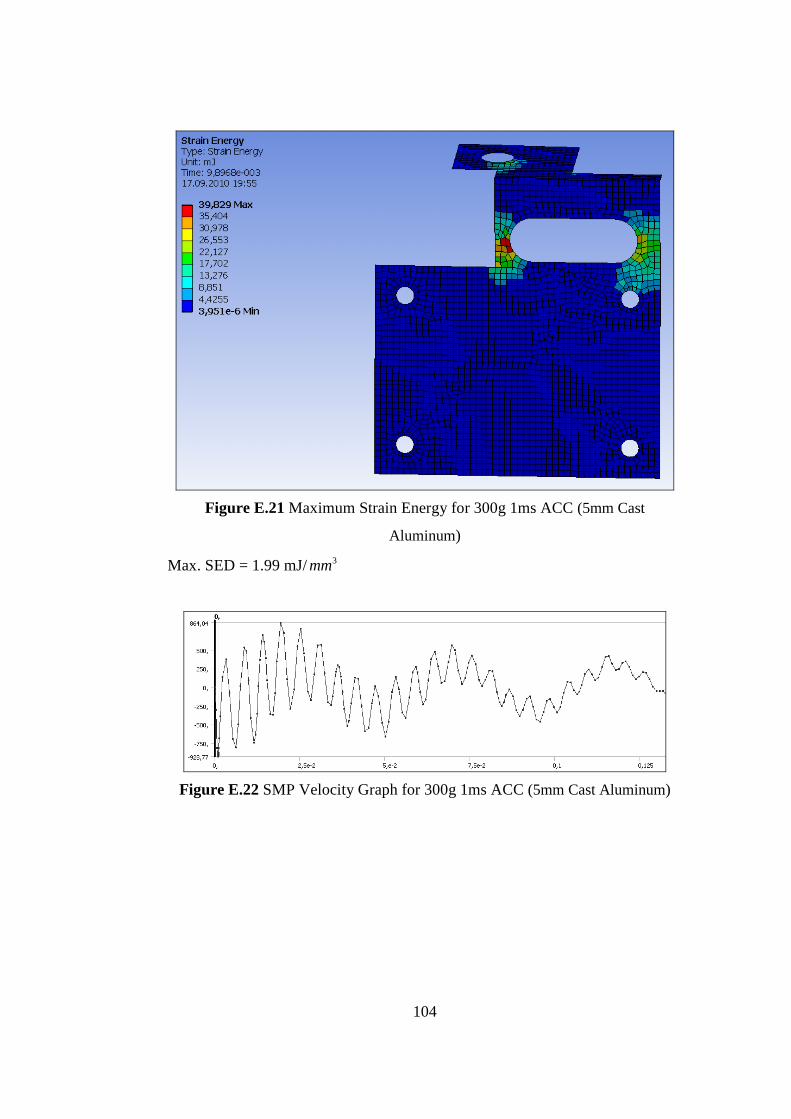
104
Figure E.21 Maximum Strain Energy for 300g 1ms ACC (5mm Cast
Aluminum)
Max. SED = 1.99 mJ/ 3mm
Figure E.22 SMP Velocity Graph for 300g 1ms ACC (5mm Cast Aluminum)
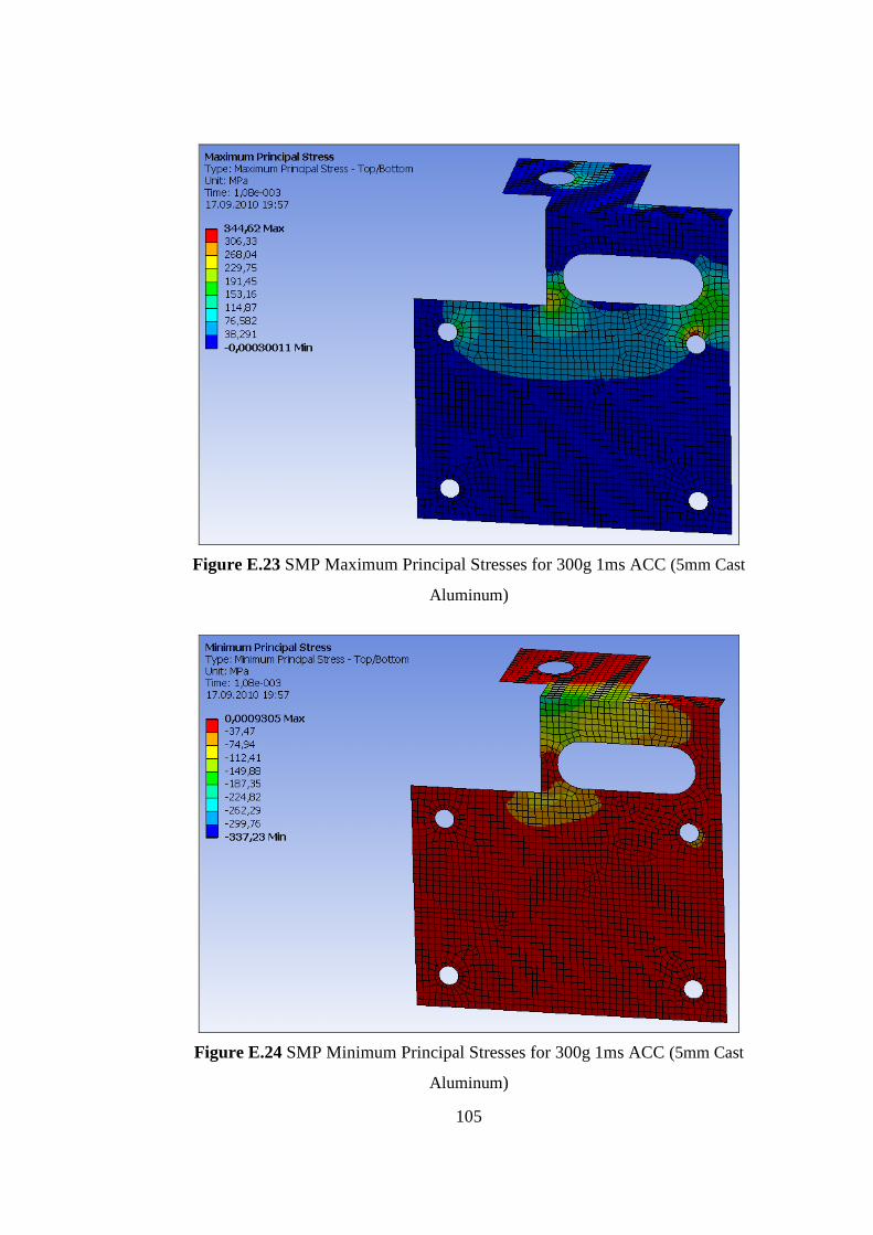
105
Figure E.23 SMP Maximum Principal Stresses for 300g 1ms ACC (5mm Cast
Aluminum)
Figure E.24 SMP Minimum Principal Stresses for 300g 1ms ACC (5mm Cast
Aluminum)
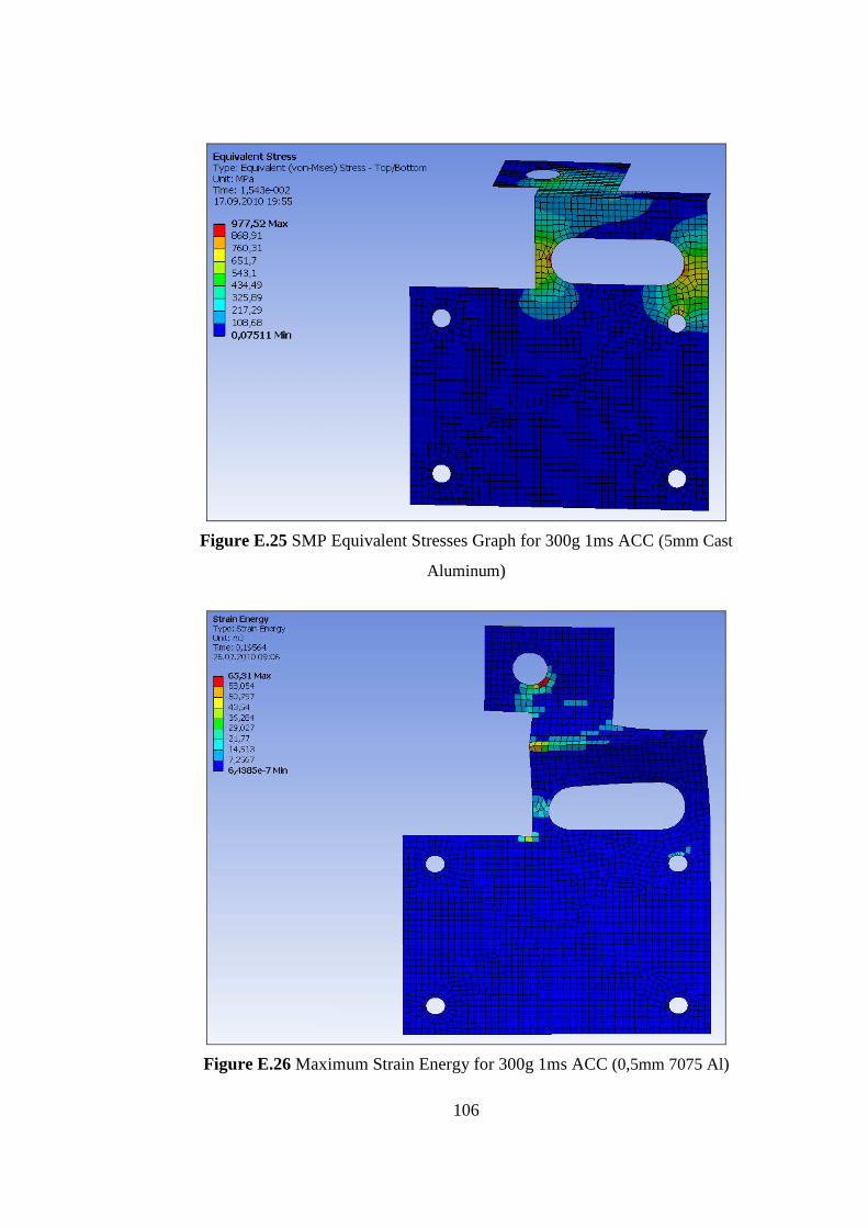
106
Figure E.25 SMP Equivalent Stresses Graph for 300g 1ms ACC (5mm Cast
Aluminum)
Figure E.26 Maximum Strain Energy for 300g 1ms ACC (0,5mm 7075 Al)
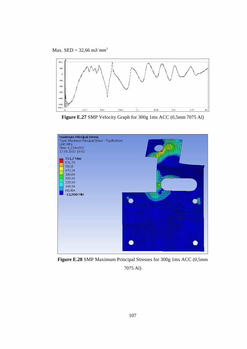
107
Max. SED = 32,66 mJ/ 3mm
Figure E.27 SMP Velocity Graph for 300g 1ms ACC (0,5mm 7075 Al)
Figure E.28 SMP Maximum Principal Stresses for 300g 1ms ACC (0,5mm
7075 Al)
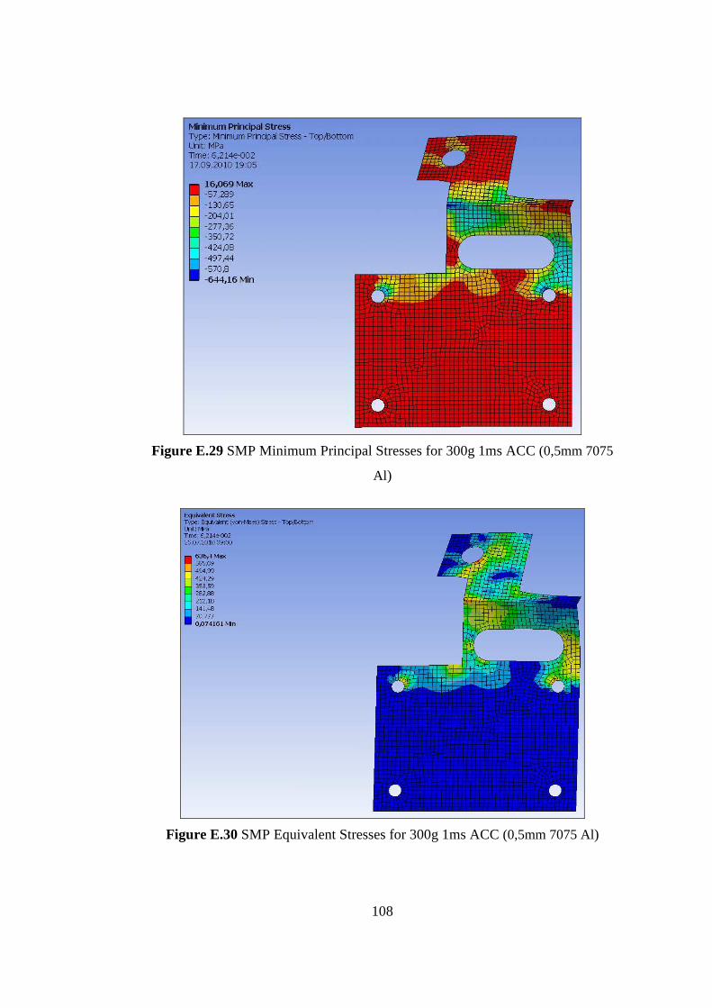
108
Figure E.29 SMP Minimum Principal Stresses for 300g 1ms ACC (0,5mm 7075
Al )
Figure E.30 SMP Equivalent Stresses for 300g 1ms ACC (0,5mm 7075 Al)

109
Figure E.31 Maximum Strain Energy for 300g 1ms ACC (1mm 7075 Al)
Max. SED = 22,64 mJ/ 3mm
Figure E.32 SMP Velocity Graph for 300g 1ms ACC (1mm 7075 Al)
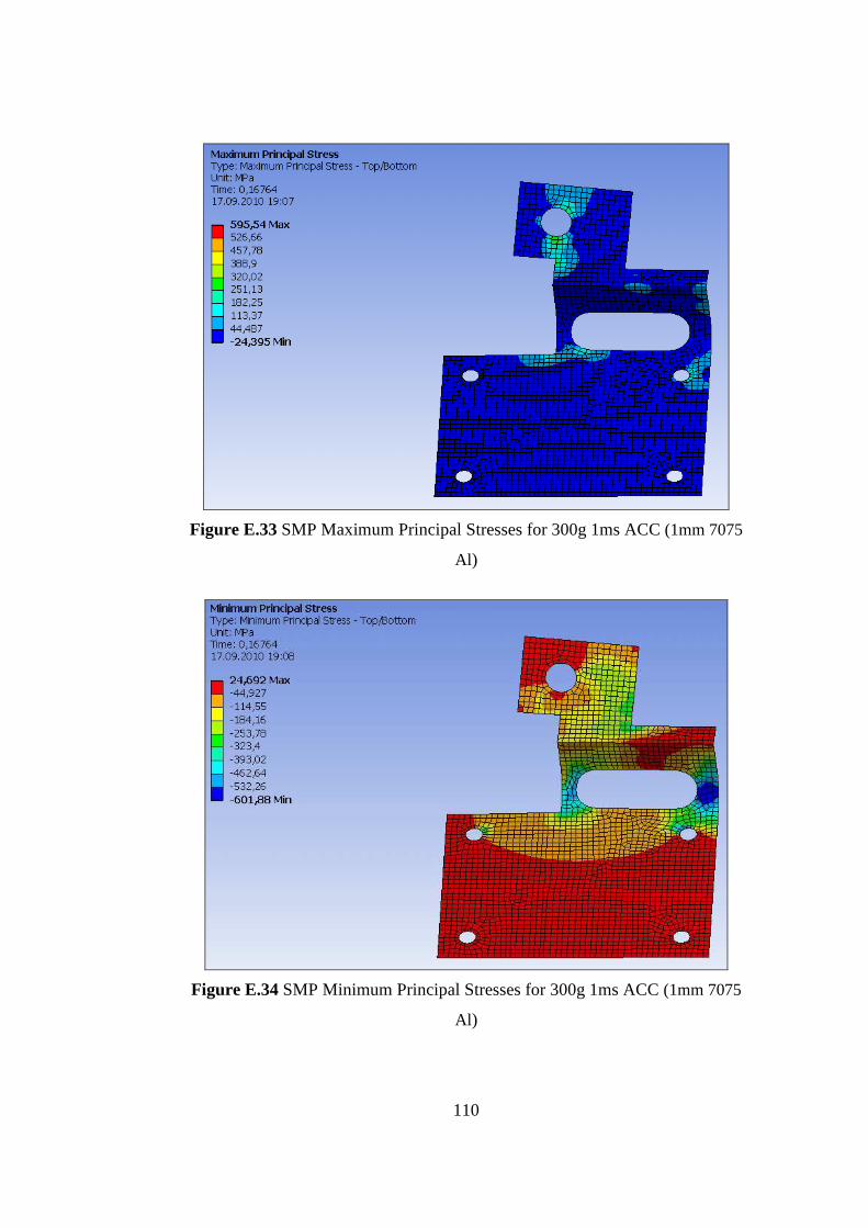
110
Figure E.33 SMP Maximum Principal Stresses for 300g 1ms ACC (1mm 7075
Al )
Figure E.34 SMP Minimum Principal Stresses for 300g 1ms ACC (1mm 7075
Al )
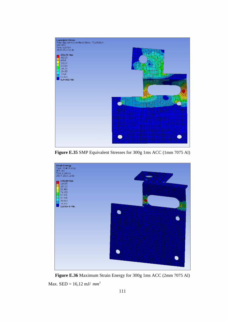
111
Figure E.35 SMP Equivalent Stresses for 300g 1ms ACC (1mm 7075 Al)
Figure E.36 Maximum Strain Energy for 300g 1ms ACC (2mm 7075 Al)
Max. SED = 16,12 mJ/ 3mm

112
Figure E.37 SMP Velocity Graph for 300g 1ms ACC (2mm 7075 Al)
Figure E.38 SMP Maximum Principal Stresses for 300g 1ms ACC (2mm 7075
Al )
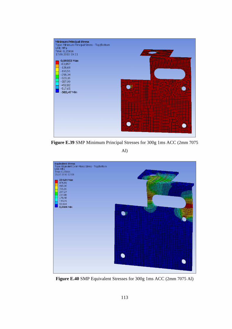
113
Figure E.39 SMP Minimum Principal Stresses for 300g 1ms ACC (2mm 7075
Al )
Figure E.40 SMP Equivalent Stresses for 300g 1ms ACC (2mm 7075 Al)

114
Figure E.41 Maximum Strain Energy for 300g 1ms ACC (3mm 7075 Al)
Max. SED = 10,66 mJ/ 3mm
Figure E.42 SMP Velocity Graph for 300g 1ms ACC (3mm 7075 Al)
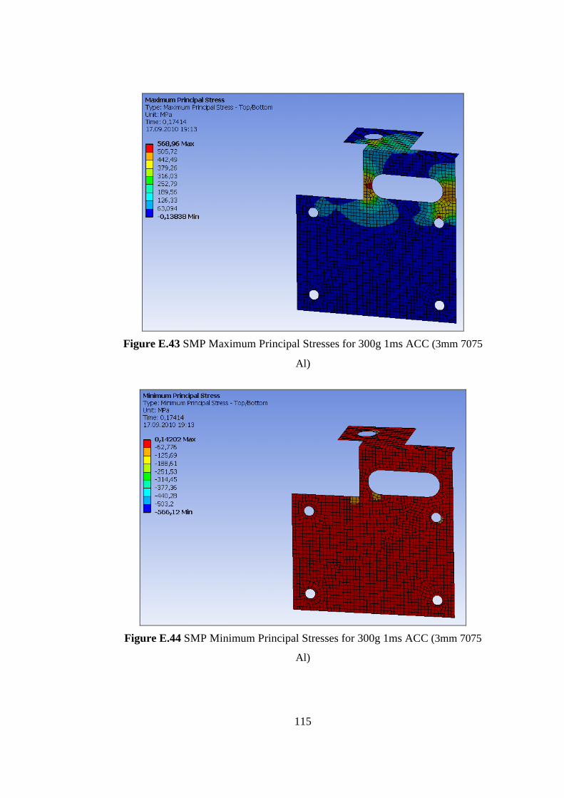
115
Figure E.43 SMP Maximum Principal Stresses for 300g 1ms ACC (3mm 7075
Al )
Figure E.44 SMP Minimum Principal Stresses for 300g 1ms ACC (3mm 7075
Al)
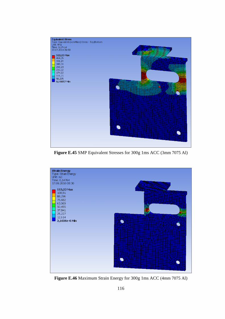
116
Figure E.45 SMP Equivalent Stresses for 300g 1ms ACC (3mm 7075 Al)
Figure E.46 Maximum Strain Energy for 300g 1ms ACC (4mm 7075 Al)
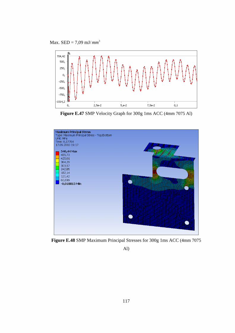
117
Max. SED = 7,09 mJ/ 3mm
Figure E.47 SMP Velocity Graph for 300g 1ms ACC (4mm 7075 Al)
Figure E.48 SMP Maximum Principal Stresses for 300g 1ms ACC (4mm 7075
Al )
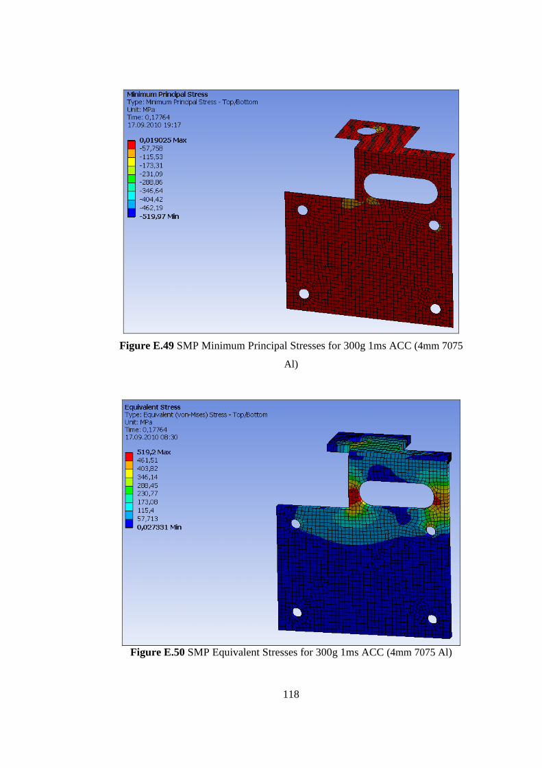
118
Figure E.49 SMP Minimum Principal Stresses for 300g 1ms ACC (4mm 7075
Al)
Figure E.50 SMP Equivalent Stresses for 300g 1ms ACC (4mm 7075 Al)
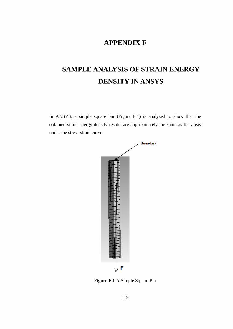
119
APPENDIX F
F. SAMPLE ANALYSIS OF STRAIN ENERGY
DENSITY IN ANSYS
In ANSYS, a simple square bar (Figure F.1) is analyzed to show that the
obtained strain energy density results are approximately the same as the areas
under the stress-strain curve.
Figure F.1 A Simple Square Bar
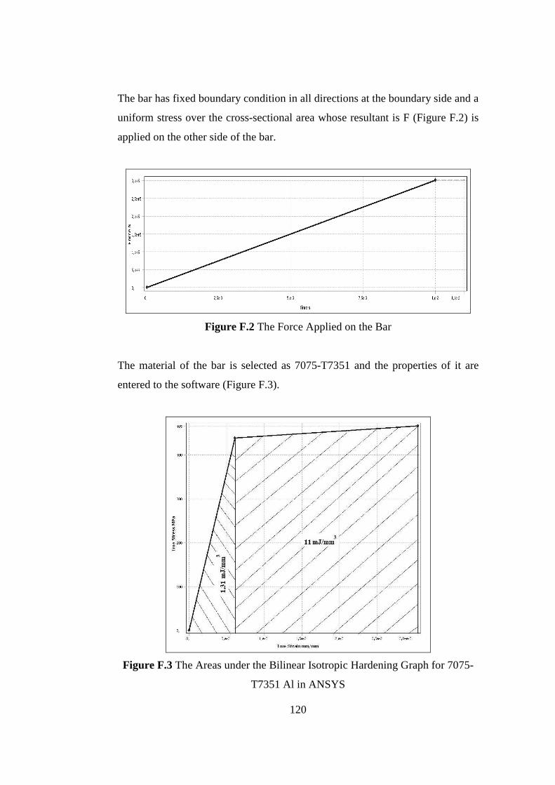
120
The bar has fixed boundary condition in all directions at the boundary side and a
uniform stress over the cross-sectional area whose resultant is F (Figure F.2) is
applied on the other side of the bar.
Figure F.2 The Force Applied on the Bar
The material of the bar is selected as 7075-T7351 and the properties of it are
entered to the software (Figure F.3).
Figure F.3 The Areas under the Bilinear Isotropic Hardening Graph for 7075-
T7351 Al in ANSYS
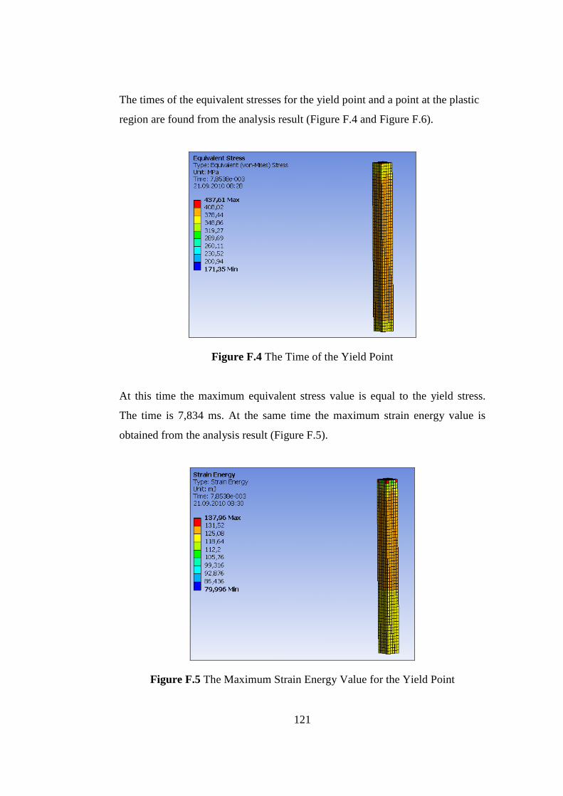
121
The times of the equivalent stresses for the yield point and a point at the plastic
region are found from the analysis result (Figure F.4 and Figure F.6).
Figure F.4 The Time of the Yield Point
At this time the maximum equivalent stress value is equal to the yield stress.
The time is 7,834 ms. At the same time the maximum strain energy value is
obtained from the analysis result (Figure F.5).
Figure F.5 The Maximum Strain Energy Value for the Yield Point
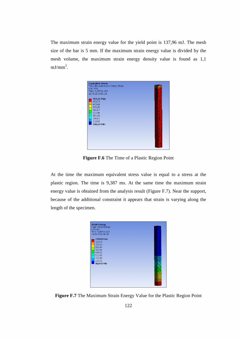
122
The maximum strain energy value for the yield point is 137,96 mJ. The mesh
size of the bar is 5 mm. If the maximum strain energy value is divided by the
mesh volume, the maximum strain energy density value is found as 1,1
mJ/mm3.
Figure F.6 The Time of a Plastic Region Point
At the time the maximum equivalent stress value is equal to a stress at the
plastic region. The time is 9,387 ms. At the same time the maximum strain
energy value is obtained from the analysis result (Figure F.7). Near the support,
because of the additional constraint it appears that strain is varying along the
length of the specimen.
Figure F.7 The Maximum Strain Energy Value for the Plastic Region Point

123
The maximum strain energy value for the plastic region point is 1339,8 mJ. The
mesh size of the bar is 5 mm. If the maximum strain energy value is divided by
the mesh volume, the maximum strain energy density value is found as 10,7
mJ/mm3.
The strain energy density results obtained by using FEM simulation are
acceptably close to the areas under the stress-strain curve. All results are given
in Table F.1.
Table F.1 Strain Energy Density Results of ANSYS for the Sample Bar
Yield Point
The Plastic Region Point
Error 100*(B-A)/B
Analysis Result for The Strain Energy Density (mJ/mm3) (A)
1,1 10,7 16%
The Area under The Stress-Strain Curve (mJ/mm3)(B)
1,31 12,31 13%
Figure F.8 Force vs Load Point Displacement Graph
The force for the yield point which is at 7,834 ms is found 236 kN by using
Figure F.2. The work done up to yield point is calculated as 185,1 J by using the
area under the force vs displacement curve (Figure F.8). On the other hand the
force for the plastic region point which is at 9,387 ms is found 282 kN and the
work done up to the point is calculated as 265 J.
The Plastic Region Point