IOP PUBLISHING NONLINEARITY

Nonlinearity 22 (2009) 1337–1366 doi:10.1088/0951-7715/22/6/005

Shock structure in continuum models of gas dynamics:stability and bifurcation analysis

Srboljub S Simic

Department of Mechanics, Faculty of Technical Sciences, University of Novi Sad, Trg DositejaObradovica 6, 21000 Novi Sad, Serbia

E-mail: ssimic@uns.ac.rs

Received 25 July 2008, in final form 11 March 2009Published 24 April 2009Online at stacks.iop.org/Non/22/1337

Recommended by L Bunimovich

AbstractThe problem of shock structure in gas dynamics is analysed through acomparative study of two continuum models: the parabolic Navier–Stokes–Fourier model and the hyperbolic system of 13 moments equations modelingviscous, heat-conducting monatomic gases within the context of extendedthermodynamics. When dissipative phenomena are neglected these modelsboth reduce to classical Euler’s equations of gas dynamics. The shock profilesolution, assumed in the form of a planar travelling wave, reduces the problemto a system of ordinary differential equations, and equilibrium states appear tobe stationary points of the system. It is shown that in both models an upstreamequilibrium state suffers an exchange of stability when the shock speed crossesthe critical value which coincides with the highest characteristic speed of theEuler’s system. At the same time a downstream equilibrium state could be seenas a steady bifurcating solution, while the shock profile represents a heteroclinicorbit connecting the two stationary points. Using centre manifold reduction itis demonstrated that both models, although mathematically different, obey thesame transcritical bifurcation pattern in the neighbourhood of the bifurcationpoint corresponding to the critical value of shock speed, the speed of sound.

Mathematics Subject Classification: 35L65, 35L67, 37G10, 34C37, 58K25

1. Introduction

Shock waves are moving singular surfaces on which jump discontinuities of field variablesoccur. In physical reality, due to dissipative mechanisms they are observed as narrow transitionregions with steep gradients of field variables within, i.e. shock waves are endowed withstructure. The shock structure problem consists of a mathematical description of this region

0951-7715/09/061337+30$30.00 © 2009 IOP Publishing Ltd and London Mathematical Society Printed in the UK 1337

1338 S S Simic

through particular solutions of appropriate mathematical models. This problem is challengingboth from the mathematical and physical points of view. Mathematically, questions of existenceand uniqueness are very important for the solutions with jump discontinuities, as well as forcontinuous ones. Physically, the continuum hypothesis becomes doubtful in this situation,thus limiting the range of validity of continuum theories of fluids.

This paper presents a contribution towards understanding common properties that may befound in descriptions of the shock structure within different continuum models of gas dynamics.It is motivated by the coexistence of the models with strikingly different mathematical structure,but pretending to describe the same phenomenon. In particular, the main issue of the studywill be stability and bifurcation analysis of equilibrium states which naturally arises withinthe framework of the shock structure problem. The models to be discussed will be: (a) Euler’sequations of gas dynamics, as a prototype of the hyperbolic system of conservation laws; (b) theNavier–Stokes–Fourier (NSF) parabolic model; (c) 13 moments equations, as a hyperbolicmodel with balance laws which arise within the context of extended thermodynamics.

Classical Euler’s equations predict the existence of shock waves as discontinuous solutionstravelling at a constant shock speed s. The jumps of field variables are related to the shockspeed through the Rankine–Hugoniot equations [8]. Since their solution is not unique, anadditional criterion has to be established in order to pick up physically admissible solutions.In this case Lax’s condition, as well as other ones, claims that admissible weak shocks are theones whose speed is supersonic with respect to the upstream equilibrium state [10, 26].

In contrast to Euler’s model where dissipation is neglected, NSF equations take dissipativemechanisms into account through the classical constitutive equations for stress tensor and heatflux. Although the resulting mathematical model is parabolic, it has solutions in the form ofa travelling wave which resemble the shock wave. They represent the shock with a structurewhich travels at a constant speed s, related to upstream and downstream equilibria throughthe same Rankine–Hugoniot equations as in Euler’s model. The existence of such solutions isdiscussed for general parabolic models [21], and for this particular one as well [12, 19]. Usinga travelling wave ansatz a system of partial differential equations (PDEs) is transformed into asystem of ordinary differential equations (ODEs). In terms of phase trajectories of dynamicalsystems, the shock structure is then described as a heteroclinic orbit which asymptoticallyconnects stationary points which correspond to equilibrium states of the model [13].

Another description of dissipative mechanisms in gas dynamics had been developed in theframework of extended thermodynamics [22]. It led to the so-called 13 moments model. Thebehaviour of nonconvective fluxes, like stress tensor and heat flux, is determined by additionalbalance laws. The differential part of the resulting system of balance laws is hyperbolic, at leastin some region of the state space, but Rankine–Hugoniot equations have a different structurethan in Euler’s case. However, travelling waves—i.e. the shocks with a structure—may beconstructed and their existence is related again to the shock waves which appear in Euler’smodel. This is in accordance with the existence result for hyperbolic systems of balancelaws [31]. As in the NSF model, travelling shock profiles can be interpreted in terms ofheteroclinic orbits connecting the same stationary points, although the ODE system governingthe trajectories is different from the NSF one.

The existence theorems, either in the parabolic, or in the hyperbolic case, relate theexistence of the shock profile to the following conditions:

(i) the upstream and downstream equilibrium states are related to the shock speed s throughRankine–Hugoniot equations for the basic (Euler’s) model with neglected dissipation;

(ii) the pair of states connected by the shock profile satisfy the appropriate shock admissibilitycriterion, e.g. Lax’s or Liu’s condition, for the basic hyperbolic system without dissipation.

Shock structure in gas dynamics 1339

In particular, admissibility condition (ii), in its various forms, stands as a necessary and/orsufficient condition for the existence of shock profiles of weak shocks in general systems ofconservation laws with viscous extensions (see [21], theorem 3.1), as well as in hyperbolicsystems with relaxation (see [31], theorem 2.2).

The aim of this study is to analyse the shock structure problem using the dynamical systemsapproach [24]. The main idea is to drop the second condition (admissibility criterion) and toanalyse the behaviour of the stationary points, i.e. upstream and downstream equilibrium states,while the shock speed is changed as a parameter. Using stability theory it will be shown thatthe stationary points change their stability properties while shock speed crosses the criticalvalue which corresponds to the upstream speed of sound, determined from Euler’s model.To be precise, one of the eigenvalues of the linearized system of ODEs describing the shockstructure changes the sign in this situation. Furthermore, using centre manifold reduction andlocal bifurcation theory it will be shown that the stationary points form two transverse branchesof solutions while the shock speed is varied. The one which corresponds to the downstreamequilibrium state may be treated as a bifurcating solution. The local structure of solutions isthen determined by the transcritical bifurcation pattern whose normal form is

y = εy − y2, (1.1)

where y stands for a generic state variable and ε is a generic bifurcation parameter. Theseresults will turn out to be valid both for the parabolic NSF model and for the hyperbolic13 moments equations, i.e. the bifurcation equation will have the same form in either case.Thus, by putting the admissibility criterion aside it will be demonstrated that the existenceof heteroclinic orbits is not a prerogative of admissible equilibrium states—they can also beobserved in the case of inadmissible ones which appear in the case of subsonic wave speed.However, the stability criterion provided in this survey selects the admissible shock structuresin dissipative models in an analogous way as the usual admissibility criteria do for shocks inEuler’s system.

Stability and bifurcation analysis related to the shock structure problem had been appliedmostly in the context of the Boltzmann equation. Nicolaenko and Thurber [23] showed that theBoltzmann operator for hard sphere potential has a nontrivial eigenvalue which changes the signin transition from the subsonic to the supersonic regimes. Moreover, they derived bifurcationequations using the Lyapunov–Schmidt reduction procedure. Caflisch and Nicolaenko [7]generalized these results for hard cut-off potentials and proved the existence of shock profilesolutions. Existence results for discrete velocity models of the Boltzmann equation, whichalso have a flavour of bifurcation theory, have been proven by Bose et al [4] and Bernhoff andBobylev [5]. Recently [19], centre manifold reduction has been applied to prove the existenceof weak shocks for the NSF model, and bifurcation equation of the transcritical type appearedthere only as a by-product. On the other hand, bifurcation theory has been successfully appliedto the analysis of the Riemann problem for viscous conservation laws [25] and bifurcation ofundercompressive and overcompressive viscous profiles from the constant state [2]. However,it seems that there is a lack of comparative analysis of dissipative models which, althoughmathematically different, should have a common ground. This study tends to fill this gap andpresents a continuation of the author’s previous work [27].

The paper will be organized as follows. In section 2 the necessary background materialabout continuum models of gas dynamics and their mathematical structure will be presented.Section 3 will contain a brief survey of the centre manifold reduction procedure needed for localstability and bifurcation analysis. Section 4 will comprise a preparatory review of the shockwave analysis for Euler’s equations. Key results on the shock structure analysis for the NSFmodel and the 13 moments equations in the light of dynamical systems theory will be presented

1340 S S Simic

in sections 5 and 6. Finally, section 7 will contain a material which explains possible furtherapplications of the method concerned with more involved mathematical models, as well assome numerical aspects of presented results.

2. Continuum models of gas dynamics

Continuum models in physics are often expressed in the form of conservation laws. Whenrestricted to one space dimension they read

∂tF0(u) + ∂xF(u) = 0, (2.1)

where u ∈ Rn, u = u(x, t), is the vector of state variables; F0(u) is the vector of densitiesand F(u) the vector of fluxes, both being smooth vector-functions in an open set of the statespace. Physically, F(u) expresses the flux of the state variables through the boundary of someregion in space and determines the rate of change of densities F0(u), i.e. the state variables init. The structure of the flux vector depends on the model of continuum adopted in a particularproblem. A classical example is the Euler’s system of gas dynamics equations

∂tρ + ∂x(ρv) = 0,

∂t (ρv) + ∂x(ρv2 − σ + p) = 0,

∂t (12ρv2 + ρe) + ∂x((

12ρv2 + ρe)v − σv + pv + q) = 0.

(2.2)

Viscous stress σ and heat flux q are neglected in this model (σ = 0, q = 0) and appear inequation (2.2) just for future reference. In what follows, the following set of state variableswill be used u = (ρ, v, T ), i.e. density, velocity and temperature. At the same time pressurep and internal energy density e are determined by the constitutive equations—thermal andcaloric equations of state of an ideal gas

p = p(ρ, T ) = RρT, e = e(ρ, T ) = RT

γ − 1, (2.3)

where R = kB/m is the gas constant (kB is Boltzmann constant, m is the atomic mass of gas)and γ the ratio of specific heats.

When densities F0(u) and fluxes F(u) are functions of state variables solely, i.e. not oftheir derivatives, it is expected that (2.1) is hyperbolic, at least in some region of the statespace. In other words, the eigenvalue problem

(−λA0(u) + A(u))r = 0;A0(u) = ∂F0(u)/∂u; A(u) = ∂F(u)/∂u,

(2.4)

has n real eigenvalues λi(u) called characteristic speeds, and n linearly independenteigenvectors ri (u), i = 1, . . . , n; A0(u) is assumed to be nonsingular. This property permitspropagation of disturbances (waves) through space with finite speeds. In the usual terminologyof hyperbolic conservation laws, λi(u) is genuinely nonlinear if (∂λi(u)/∂u) · ri (u) �= 0 forall u, while it is linearly degenerate if (∂λi(u)/∂u) · ri (u) = 0 for all u.

Hyperbolicity is the main cause of nonexistence of smooth solutions for all t , even wheninitial data are smooth. Jump discontinuities, i.e. shock waves, which are located on the surfaceof discontinuity �(x, t), may appear in a finite time interval. If [[·]] = (·)1 − (·)0 denotes thejump of any quantity in front (·)0 and behind (·)1 the surface �, then Rankine–Hugoniotconditions relate the jump of the field variables to the speed of shock s

[[F(u)]] = s[[F0(u)]]. (2.5)

However, not all of the jump discontinuities which satisfy (2.5) are observable in reality(at least in the approximate sense). Along with Rankine–Hugoniot conditions, they have to

Shock structure in gas dynamics 1341

satisfy additional ones which serve as selection rules for physically admissible solutions. Areview of these conditions may be found in [10, 26]. For the purpose of this exposition weshall be confined with the Lax condition

λi(u1) � s � λi(u0). (2.6)

The study will be restricted to classical compressive i-shocks for which strict inequalities in(2.6) hold. In such a case the Lax condition represents a particular form of irreversibilitycondition since the roles of u0 and u1 cannot be interchanged [10]. A similar restriction comesfrom the entropy shock admissibility condition which puts this problem on a sound physicalground, but it is equivalent to (2.6) for weak i-shocks under certain assumptions.

Euler’s equations (2.2) are equipped with the following set of characteristic speeds

λ1 = v − cs; λ2 = v; λ3 = v + cs; (2.7)

cs = (γRT )1/2, (2.8)

where cs is the local speed of sound; λ1 and λ3 are genuinely nonlinear, whereas λ2 is linearlydegenerate. Lax condition (2.6) states that shock waves have to be supersonic w.r.t. theupstream state u0 = (ρ0, v0, T0) in front of them, and subsonic w.r.t. the downstream stateu1 = (ρ1, v1, T1) behind them.

A flavour of bifurcation theory in the analysis of shock waves had been captured in thepaper of Lax [18]. It may be outlined through the following observation. First, it is obviousthat (2.5) has trivial solution u1 = u0 for any value of shock speed. Second, it may be shown bymeans of the implicit function theorem (see [22], p.189) that uniqueness of the trivial solutionis lost when s = λi(u0). Actually, Lax has shown that solution u1 �= u0 of equation (2.5)belongs to the set of points known as the Hugoniot locus of u0 [10], thus representing thei-shock. Therefore, u1 may be regarded as a bifurcating solution when shock speed crossesthe critical value s∗ = λi(u0) = λi(u1).

Existence of shock waves is an intrinsic property of hyperbolic systems of conservationlaws such as (2.1). In reality they are recognized as narrow transition regions in theneighbourhood of surface of discontinuity �(x, t) where steep gradients of the state variablesoccur, rather than their jumps. In such a way shock is endowed with the structure due to thepresence of dissipative mechanisms, and a shock profile is observed instead of a shock wave.

Regularizing effects of dissipation can be modelled in several ways. Classical continuummechanics motivates the so-called viscosity approach which regularizes system (2.1) by addingparabolic terms

∂tF0(u) + ∂xF(u) = ε∂x(B(u)∂xu), (2.9)

where B(u) is the viscosity matrix and ε ∈ R+ a small parameter. This model predicts infinitespeed of propagation of disturbances, and characteristic speeds, as one of the basic features ofa hyperbolic model (2.1), cannot be related to (2.9). However, parabolic terms regularize theshock waves which correspond to genuinely nonlinear characteristic speeds of (2.1). In sucha way (2.9) comprises solutions representing the shock profile travelling uniformly with theshock speed s. For example, Euler’s equations (2.2) are regularized when viscosity and heatconduction are taken into account through Navier–Stokes and Fourier constitutive equations

σ = 43µ∂xv, q = −κ∂xT , (2.10)

1342 S S Simic

where µ is viscosity of a gas and κ its heat conductivity (µ, κ > 0). Consequently, the NSFmodel of gas dynamics reads

∂tρ + ∂x(ρv) = 0,

∂t (ρv) + ∂x(ρv2 + p) = ∂x(43µ∂xv),

∂t (12ρv2 + ρe) + ∂x((

12ρv2 + ρe)v + pv)

= ∂x(κ∂xT + 43µv∂xv).

(2.11)

General considerations about the viscosity approach to weak shocks in systems of conservationlaws are presented by Majda and Pego [21]. Existence and uniqueness of shock profile solutionsfor the NSF model (2.11) had been studied successfully by Gilbarg [12] for a rather generalclass of fluids where µ and κ are arbitrary functions of state variables.

Another way of describing dissipative mechanisms is to take into account the relaxationeffects. Formally, this calls for extension of the set of state variables u ∈ Rn by v ∈ Rk ,n + k = N , which are governed by the additional set of balance laws. In particular, we have

∂t F0(U) + ∂xF(U) = 1

τQ(U), (2.12)

where

U =(

u

v

), Q(U) =

(0

q(u, v)

),

F0(U) =

(f0(u, v)

g0(u, v)

), F(U) =

(f(u, v)

g(u, v)

),

(2.13)

and τ ∈ R+ is a small parameter. It is assumed that q(u, v) = 0 uniquely determines ‘theequilibrium manifold’ vE = h(u) as τ → 0, on which system (2.12) reduces to (2.1) withF0(u) = f0(u, h(u)) and F(u) = f(u, h(u)). In (2.12) the first n equations are conservationlaws, while the remaining k ones are balance laws with source terms q(u, v)/τ which describethe dissipative effects out of the equilibrium manifold.

It is customary to expect that system (2.12) is hyperbolic at least in some subset ofthe extended state space RN which contains the equilibrium manifold. Correspondingcharacteristic speeds �j(U), j = 1, . . . , N , and the set of linearly independent eigenvectorsRj (U) are determined from the eigenvalue problem for the differential part of (2.12)

(−�A0(U) + A(U))R = 0;

A0(U) = ∂F

0(U)/∂U; A(U) = ∂F(U)/∂U.

(2.14)

An important property of characteristic speeds �j(U) is that they provide bounds for thecharacteristic speeds of (2.1) on equilibrium manifold through the subcharacteristic condition

min1�j�N

�j(u, h(u)) � λi(u) � max1�j�N

�j(u, h(u)). (2.15)

However, the spectrum λi(u) of system (2.1) does not have to be contained in the spectrum�j(u, h(u)) of the hyperbolic dissipative system (2.12), i.e. λ’s may not coincide with �’s onthe equilibrium manifold. Moreover, Rankine–Hugoniot conditions for (2.12) have a differentform than for (2.1), and consequently may predict jump discontinuities which appear off theequilibrium manifold. These discrepancies between hyperbolic systems and their dissipativecounterparts call for the answer to the question of how one can relate the jump discontinuitiesof (2.1) to the shock structure solutions expected to be derived from (2.12). First results may

Shock structure in gas dynamics 1343

be found in the work of Liu [20] for systems of two balance laws. The general existence resulthas been given by Yong and Zumbrun [31], under certain reasonable structural conditions.

In physical examples nonequilibrium variables v usually represent nonconvective fluxessuch as stress tensor or heat flux, or even higher order moments in the framework of thekinetic theory of gases. The main example which we shall examine is the hyperbolic model ofviscous, heat-conducting monatomic gas (γ = 5/3) obtained within the context of extendedthermodynamics [22] and known as the 13 moments model. This model is the same as the 13moments model of Grad [14] obtained in the kinetic theory of gases using a different closureprocedure. Governing equations of this model have the form

∂tρ + ∂x(ρv) = 0,

∂t (ρv) + ∂x(ρv2 − σ + p) = 0,

∂t

(1

2ρv2 + ρe

)+ ∂x

((1

2ρv2 + ρe

)v − σv + pv + q

)= 0,

∂t

(ρv2 + p − σ

)+ ∂x

(ρv3 + 3pv − 3σv +

6

5q

)= 1

τσ

σ,

∂t

(1

2ρv3 +

5

2pv − σv + q

)

+∂x

(1

2ρv4 + 4pv2 − 5

2σv2 +

16

5qv − 7

2

p

ρσ +

5

2

p2

ρ

)

= − 1

τq

(q − 3

2σv

).

(2.16)

In this model stress σ and heat flux q are governed by the last two balance laws rather thanconstitutive equations (2.10). Small parameters τσ and τq play the role of relaxation timesand, for monatomic gases, obey the relation τq = 3τσ /2. Although the models (2.11) and(2.16) are principally different, they are related to each other through the Chapman–Enskogexpansion. Moreover, constitutive equations (2.10) can be recovered from balance laws of(2.16) by means of the Maxwellian iteration procedure (see [22]). Either of these methodsleads to the following relations

τσ = µ

p, τq = 2

5

κ

p2ρT , κ = 15

4Rµ, (2.17)

valid for monatomic gases.Equilibrium manifold for the 13 moments system (2.16) is determined by vE = (σE, qE) =

(0, 0). Therefore, on vE this system is reduced to the so-called equilibrium subsystem ofthe Euler’s equations (2.2). The model (2.16) has five distinct characteristic speeds. Whencalculated in equilibrium and expressed in terms of sound speed (2.8) for monatomic gases(γ = 5/3) they read

�1 = v − 1.6503cs; �2 = v − 0.6297cs;�3 = v;�4 = v + 0.6297cs; �5 = v + 1.6503cs.

(2.18)

All of them are genuinely nonlinear except �3 which is linearly degenerate. Obviously,characteristic speeds (2.7) and (2.18) satisfy the subcharacteristic condition (2.15) on theequilibrium manifold with strict inequalities.

In stability and bifurcation analysis in sections 4–6 we shall be concerned with the models(2.2), (2.11) and (2.16).

1344 S S Simic

3. Centre manifold reduction

To recognize the type of bifurcation which appears in a particular problem one does nothave to analyse the behaviour of the whole set of state variables. Instead, the dimension ofthe state space can be reduced so that the reduced system comprises all the features of theoriginal one in the neighbourhood of the critical point. The centre manifold theorem providesa systematic procedure for reducing the dimension of the state space. The theorem and someof its consequences useful for further analysis will be presented in this section. Although someof the symbols used here coincide with the ones from the previous section, there is no relationbetween them whatsoever.

Consider a dynamical system

x = X(x), x ∈ Rn, (3.1)

and assume x = 0 is its stationary point, X(0) = 0. Let A = DX(0) be the Jacobian matrix. Itsspectrum could be divided into three parts—stable σs, centre σc and unstable σu—dependingon the sign of the real part of the eigenvalue λ

λ ∈ σs if Re λ < 0;λ ∈ σc if Re λ = 0;λ ∈ σu if Re λ > 0.

(3.2)

Denote by Es, Ec and Eu eigenspaces of σs, σc and σu, respectively. Then the following centremanifold theorem holds [16].

Theorem 3.1. Let X(x) be a Cr vector function on Rn, X(0) = 0. Then there exist Cr stableand unstable invariant manifolds W s and W u tangent to Es and Eu at 0 and a Cr−1 centremanifold W c tangent to Ec at 0. The manifolds W s, W u and W c are all invariant for trajectoriesof system (3.1).

In order to enable effective calculation of the centre manifold, needed to determine thebifurcation pattern, a local coordinate chart has to be chosen. Assume that x = (y, z), y ∈ Rk ,z ∈ Rm, k + m = n, puts the linear part of (3.1) at 0 into block diagonal form

y = By + Y(y, z);z = Cz + Z(y, z),

(3.3)

where B and C are constant square matrices whose eigenvalues have zero and nonzero realparts, respectively, and Y and Z vanish along with their first derivatives at 0. Since the centremanifold is tangent to Ec it can be represented as

W c = {(y, z) : z = h(y)}; h(0) = 0, Dh(0) = 0, (3.4)

where h(y) is defined in some neighbourhood of 0 ∈ Rk . Therefore, dynamics of system (3.3)can be reduced to W c in the neighbourhood of the origin by means of the following equation:

y = By + Y(y, h(y)). (3.5)

The actual form of h(y) is determined from the equation for z in (3.3)

Dh(y)[By + Y(y, h(y))

] − Ch(y) + Z(y, h(y)) = 0, (3.6)

along with boundary conditions h(0) = 0, Dh(0) = 0. The system of PDEs (3.6) can hardlybe solved exactly. However, h(y) can usually be approximated to a desired degree of accuracyby Taylor series expansion at y = 0.

Shock structure in gas dynamics 1345

The importance of centre manifold could be illustrated by a simple example (see [16]).For a two-dimensional system

y = yz; z = −z − y2, (3.7)

tangent space approximation z = h(y) = 0, motivated by the fact that z → 0 as t → ∞ inlinear approximation, leads to y = 0 which does not provide any information about stabilitynear the origin 0. However, second order centre manifold approximation

z = h(y) = −y2 + O(y4) (3.8)

determines the reduced system

y = −y3 + O(y5) (3.9)

which shows that 0 is a stable stationary point.Centre manifold reduction can also be applied to systems which contain parameters. For

simplicity assume that (3.1) depends upon a single parameter ε ∈ R. Application of the centremanifold theorem is devised through the simple extension of system (3.3)

y = Bεy + Yε(y, z);z = Cεz + Zε(y, z);ε = 0.

(3.10)

It has a k + 1-dimensional centre manifold tangent to (y, ε) space which may be approximatedby z = h(y, ε). This is standard procedure for calculating the bifurcation equation. For detailsabout this suspension method and references to original papers see [16].

4. Shock waves in Euler’s equations

The first step in the analysis will be the solution of Rankine–Hugoniot equations (2.5) forEuler’s system (2.2). It is motivated by the fact that the shock structure is a continuoussolution which connects equilibrium states. These equilibrium states are, on the other hand,related by Rankine–Hugoniot conditions for jump discontinuities.

Introducing relative velocity u = v − s, equation (2.5) for the Euler’s system may betransformed into

[[ρu]] = 0;[[ρu2 + p]] = 0;[[( 1

2ρu2 + ρε)u + pu]] = 0.

(4.1)

Using constitutive equations (2.3), the following nontrivial solution is obtained [8]:

ρ1

ρ0= M2

0

1 − µ2(1 − M20 )

;u1

u0= 1

M20

[1 − µ2(1 − M20 )];

T1

T0= 1

M20

[(1 − µ2(1 − M20 ))((1 + µ2)M2

0 − µ2)],

(4.2)

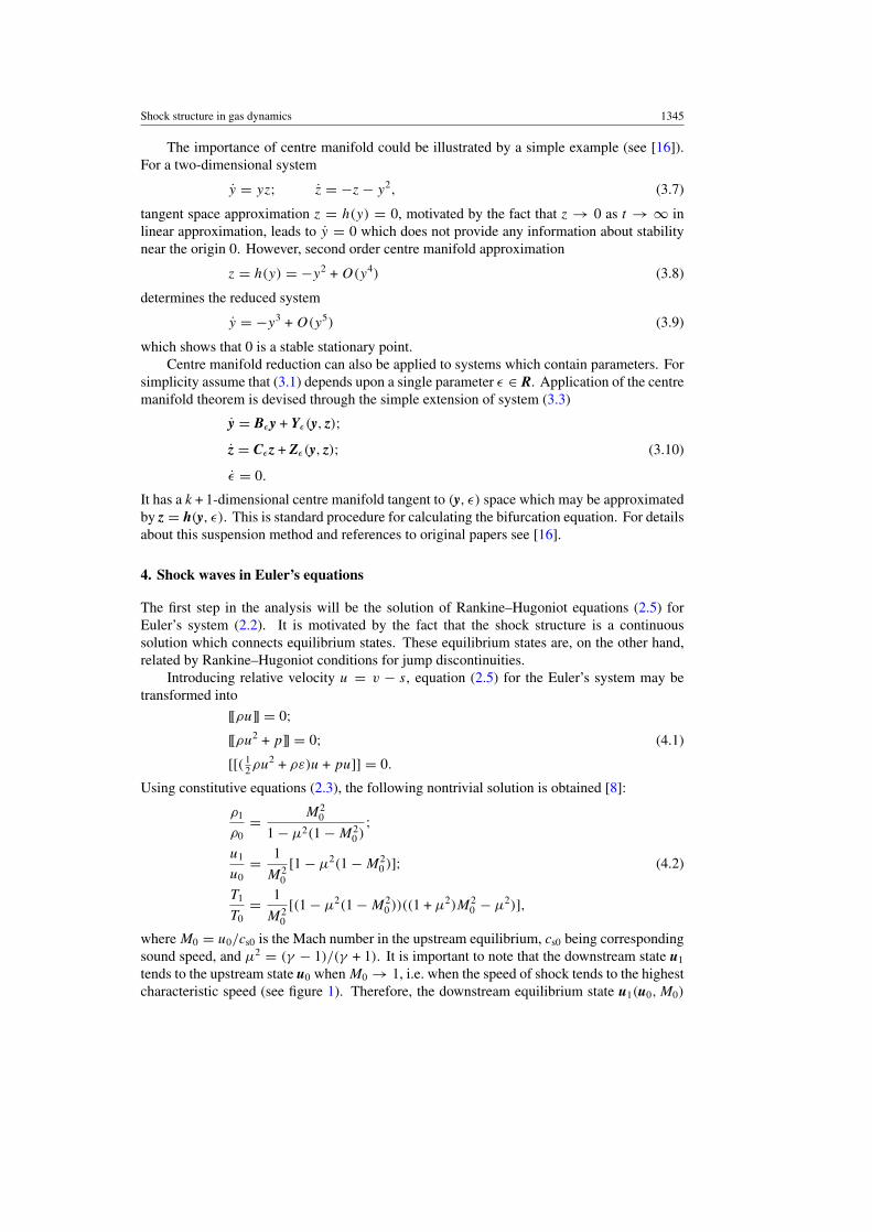
where M0 = u0/cs0 is the Mach number in the upstream equilibrium, cs0 being correspondingsound speed, and µ2 = (γ − 1)/(γ + 1). It is important to note that the downstream state u1

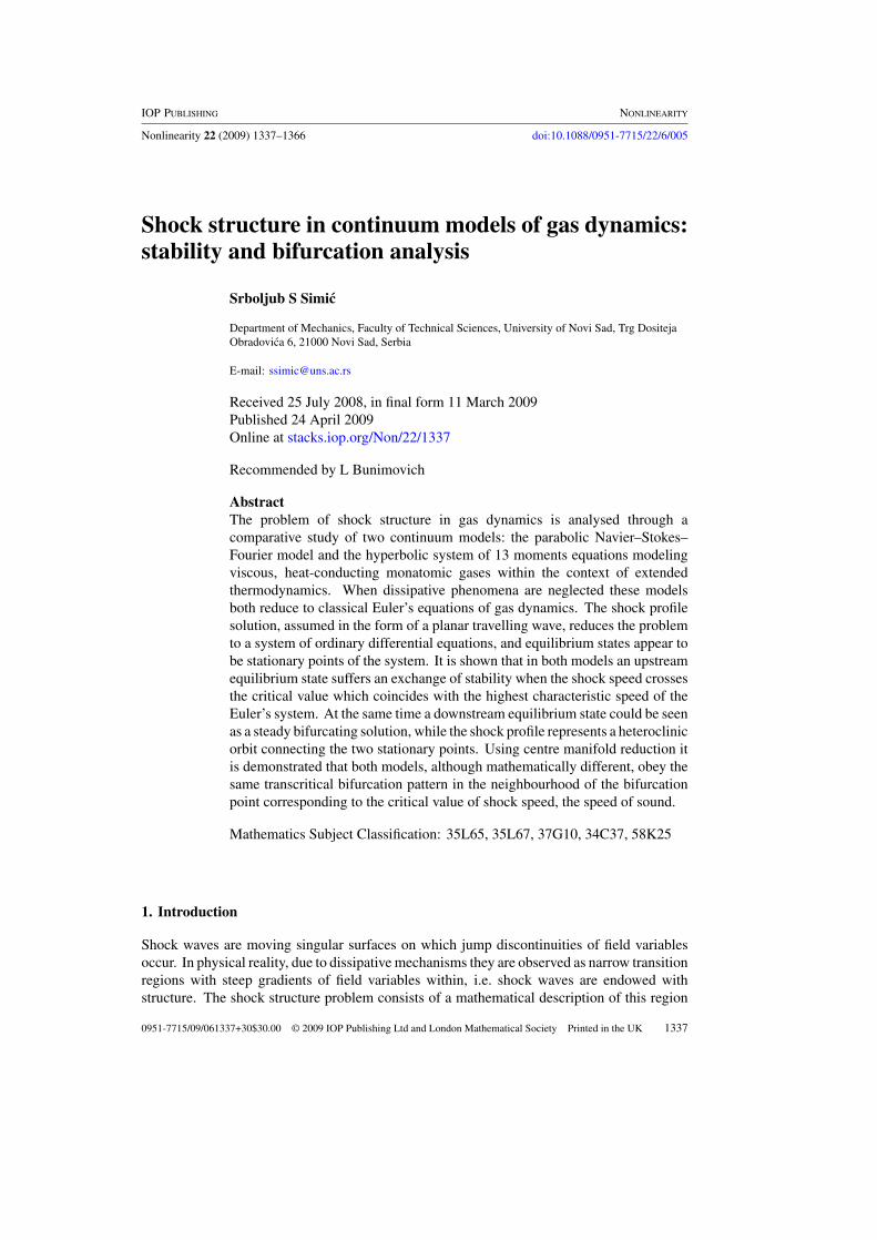
tends to the upstream state u0 when M0 → 1, i.e. when the speed of shock tends to the highestcharacteristic speed (see figure 1). Therefore, the downstream equilibrium state u1(u0, M0)

1346 S S Simic

Figure 1. Solution of Rankine–Hugoniot equations for Euler’s model (γ = 5/3).

can be regarded as a bifurcating solution, which is transverse to the trivial branch u0 in theneighbourhood of the critical point M0 = 1. Note also that, according to Lax’s condition (2.6),only the supersonic nontrivial branch (M0 > 1) is physically admissible, whereas for M0 < 1the trivial branch (u1 = u0) is an admissible one.

5. Stability and bifurcation of equilibrium in NSF model

Since shock structure is regarded as a travelling wave which moves with the speed of shock s,the solution of the problem in the case of the parabolic dissipative model (2.9) will be assumedin the form u(x, t) = u(ξ), ξ = (x − st)/ε. In such a way the system of PDEs is reduced tothe ODE system

(−sA0(u) + A(u))dudξ

= d

dξ

(B(u)

dudξ

), (5.1)

where the small parameter ε disappeared due to scaling of the independent variable. It canbe further simplified when the profile is considered in the frame of reference moving with ashock. Due to Galilean invariance of governing equations, the problem becomes stationary byintroducing the relative velocity u = v − s and equation (5.1) is reduced to

A(u)dudξ

= dF(u)

dξ= d

dξ

(B(u)

dudξ

), (5.2)

which can be integrated to obtain

B(u)dudξ

= F(u) − F(u0). (5.3)

This set of ODEs is accompanied by boundary conditions

u(−∞) = u0; u(∞) = u1;du(±∞)

dξ= 0,

(5.4)

where u0 and u1 are related through Rankine–Hugoniot equations (2.5). Equilibrium statesu0 and u1 thus represent the stationary points of system (5.3) and the shock structure is aheteroclinic orbit connecting them.

Shock structure in gas dynamics 1347

5.1. Shock structure equations

The study of the shock structure problem in the NSF model will commence with the assumptionthat viscosity is not constant, but the power-law function of the temperature

µ = µ0(T /T0)α, (5.5)

where the exponent α depends on the type of gas in consideration and µ0 is viscosity in thereferent state, here being the upstream equilibrium. For the purpose of comparison, analysiswill be restricted to the case of monatomic gases (γ = 5/3). The problem will be consideredin a moving reference frame with a single independent variable ξ = x − st . The model willbe put into dimensionless form using nondimensional quantities

ξ = ξ

l0; ρ = ρ

ρ0; u = v − s

c0; T = T

T0; (5.6)

M0 = v0 − s

c0; c0 =

(5

3RT0

)1/2

; l0 = µ0

ρ0RT0c0,

where c0 is the speed of sound in the upstream equilibrium and M0 the corresponding Machnumber. Reference length l0 is related to the mean free path of gas atoms λ through

λ =√

3

5

16

5√

2πl0 ≈ 0.989l0, (5.7)

which is quite desirable for numerical purposes and could give an indication about relationbetween shock thickness and mean free path. For the sake of simplicity tildes will be droppedin the following text.

Dimensionless equations describing the shock structure have the following form

d

dξ(ρu) = 0;

d

dξ

(5

3ρu2 + ρT

)= d

dξ

(4

3T α du

dξ

);

d

dξ

(5

6ρu3 +

5

2ρT u

)= d

dξ

(4

3T αu

du

dξ+

9

4T α dT

dξ

).

(5.8)

This system could be integrated once to obtain

ρu = M0;5

3(ρu2 − M0) + ρT − 1 = 4

3T α du

dξ;

5

6(ρu3 − M3

0 ) +5

2(ρT u − M0) = 4

3T αu

du

dξ+

9

4T α dT

dξ,

(5.9)

where dimensionless upstream equilibrium values

ρ0 = 1; u0 = M0; T0 = 1, (5.10)

have been used. Eliminating ρ by the use of mass conservation, the following system of twofirst-order ODEs is obtained

du

dξ= FP(u, T , M0) = 1

4T α

(−3 − 5M2

0 + 3M0T

u+ 5M0u

);

dT

dξ= GP(u, T , M0) = − 2

27T α(5M0(3 + M2

0 ) − 9M0T

−2(3 + 5M20 )u + 5M2

0 u2).

(5.11)

1348 S S Simic

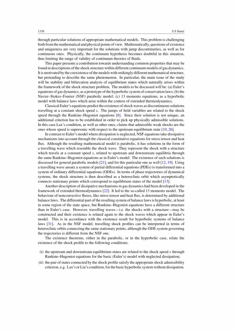
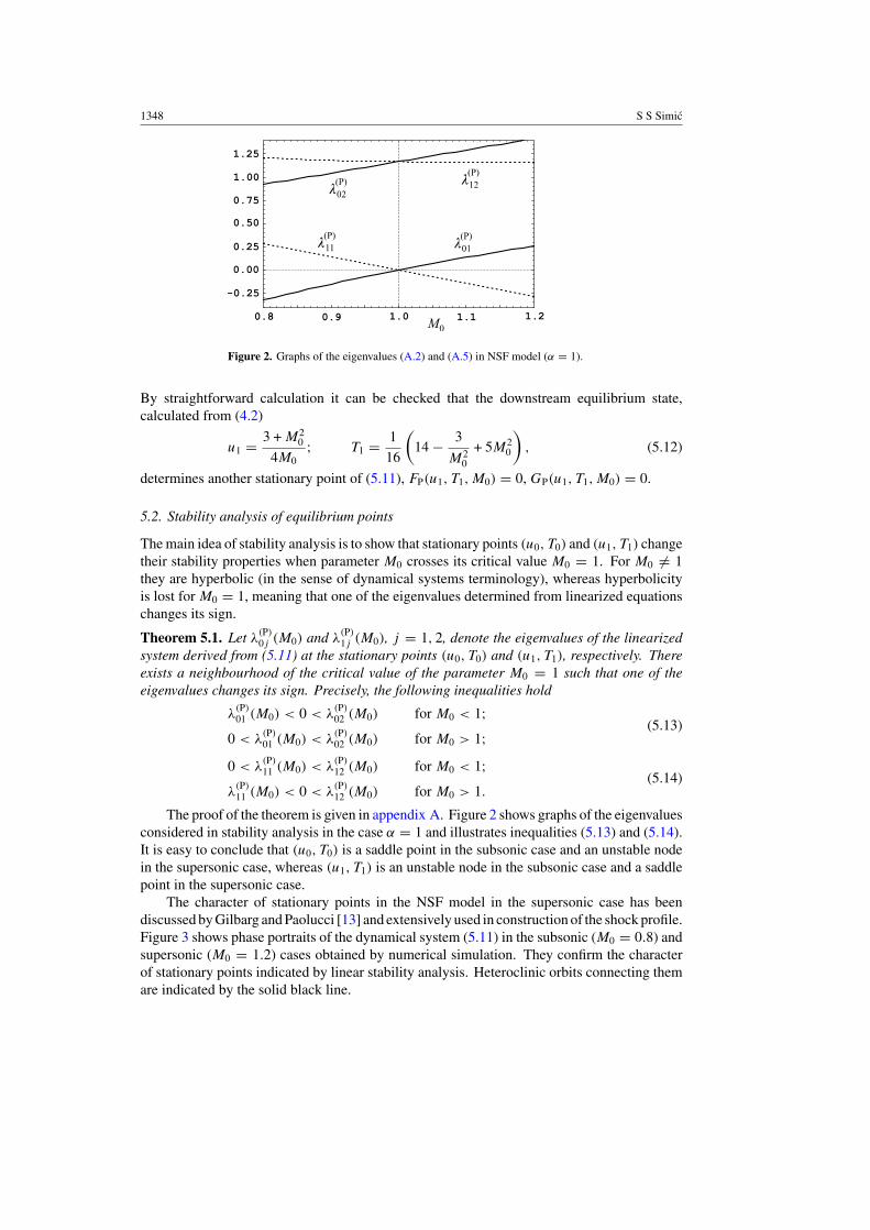
Figure 2. Graphs of the eigenvalues (A.2) and (A.5) in NSF model (α = 1).

By straightforward calculation it can be checked that the downstream equilibrium state,calculated from (4.2)

u1 = 3 + M20

4M0; T1 = 1

16

(14 − 3

M20

+ 5M20

), (5.12)

determines another stationary point of (5.11), FP(u1, T1, M0) = 0, GP(u1, T1, M0) = 0.

5.2. Stability analysis of equilibrium points

The main idea of stability analysis is to show that stationary points (u0, T0) and (u1, T1) changetheir stability properties when parameter M0 crosses its critical value M0 = 1. For M0 �= 1they are hyperbolic (in the sense of dynamical systems terminology), whereas hyperbolicityis lost for M0 = 1, meaning that one of the eigenvalues determined from linearized equationschanges its sign.

Theorem 5.1. Let λ(P)0j (M0) and λ

(P)1j (M0), j = 1, 2, denote the eigenvalues of the linearized

system derived from (5.11) at the stationary points (u0, T0) and (u1, T1), respectively. Thereexists a neighbourhood of the critical value of the parameter M0 = 1 such that one of theeigenvalues changes its sign. Precisely, the following inequalities hold

λ(P)01 (M0) < 0 < λ

(P)02 (M0) for M0 < 1;

0 < λ(P)01 (M0) < λ

(P)02 (M0) for M0 > 1;

(5.13)

0 < λ(P)11 (M0) < λ

(P)12 (M0) for M0 < 1;

λ(P)11 (M0) < 0 < λ

(P)12 (M0) for M0 > 1.

(5.14)

The proof of the theorem is given in appendix A. Figure 2 shows graphs of the eigenvaluesconsidered in stability analysis in the case α = 1 and illustrates inequalities (5.13) and (5.14).It is easy to conclude that (u0, T0) is a saddle point in the subsonic case and an unstable nodein the supersonic case, whereas (u1, T1) is an unstable node in the subsonic case and a saddlepoint in the supersonic case.

The character of stationary points in the NSF model in the supersonic case has beendiscussed by Gilbarg and Paolucci [13] and extensively used in construction of the shock profile.Figure 3 shows phase portraits of the dynamical system (5.11) in the subsonic (M0 = 0.8) andsupersonic (M0 = 1.2) cases obtained by numerical simulation. They confirm the characterof stationary points indicated by linear stability analysis. Heteroclinic orbits connecting themare indicated by the solid black line.

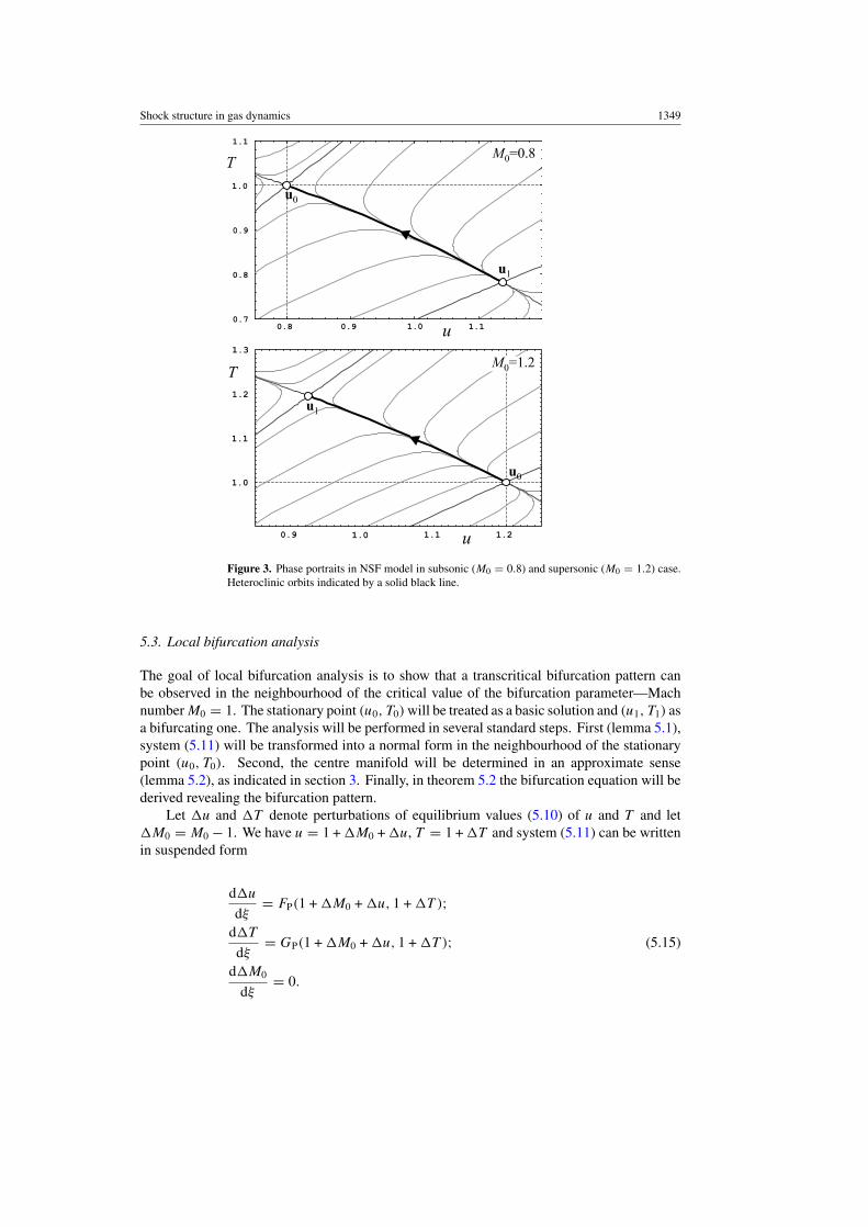
Shock structure in gas dynamics 1349

Figure 3. Phase portraits in NSF model in subsonic (M0 = 0.8) and supersonic (M0 = 1.2) case.Heteroclinic orbits indicated by a solid black line.

5.3. Local bifurcation analysis

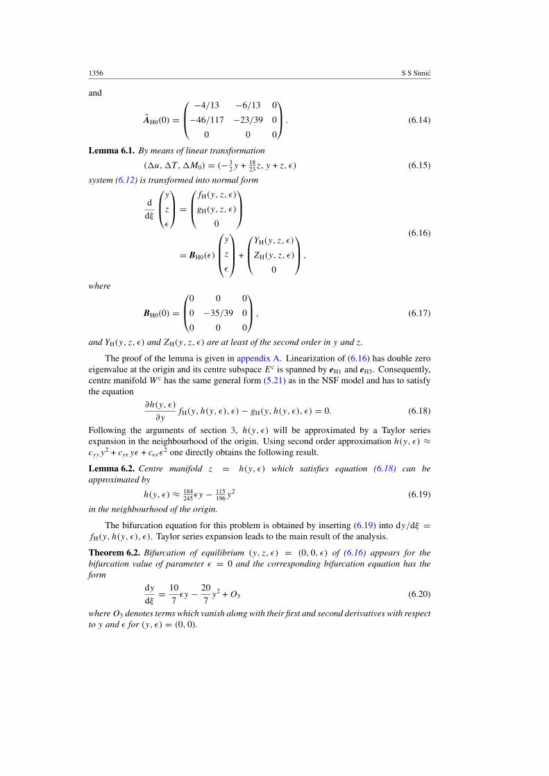
The goal of local bifurcation analysis is to show that a transcritical bifurcation pattern canbe observed in the neighbourhood of the critical value of the bifurcation parameter—Machnumber M0 = 1. The stationary point (u0, T0) will be treated as a basic solution and (u1, T1) asa bifurcating one. The analysis will be performed in several standard steps. First (lemma 5.1),system (5.11) will be transformed into a normal form in the neighbourhood of the stationarypoint (u0, T0). Second, the centre manifold will be determined in an approximate sense(lemma 5.2), as indicated in section 3. Finally, in theorem 5.2 the bifurcation equation will bederived revealing the bifurcation pattern.

Let �u and �T denote perturbations of equilibrium values (5.10) of u and T and let�M0 = M0 − 1. We have u = 1 + �M0 + �u, T = 1 + �T and system (5.11) can be writtenin suspended form

d�u

dξ= FP(1 + �M0 + �u, 1 + �T );

d�T

dξ= GP(1 + �M0 + �u, 1 + �T );

d�M0

dξ= 0.

(5.15)

1350 S S Simic

Linearization of (5.15) at (�u, �T, �M0) = (0, 0, �M0) reads

AP0(�M0) =(

AP0(1 + �M0) 0

0 0

), (5.16)

and

AP0(0) =

1/2 3/4 0

4/9 2/3 0

0 0 0

. (5.17)

Lemma 5.1. By means of linear transformation

(�u, �T, �M0) = (− 32y + 9

8z, y + z, ε) (5.18)

system (5.15) is transformed into normal form

d

dξ

y

z

ε

=

fP(y, z, ε)

gP(y, z, ε)

0

= BP0(µ)

y

z

ε

+

YP(y, z, ε)

ZP(y, z, ε)

0

,

(5.19)

where

BP0(0) =

0 0 0

0 7/6 0

0 0 0

, (5.20)

and YP(y, z, ε) and ZP(y, z, ε) vanish along with their first derivatives at (0, 0, ε).

The proof of the lemma is given in appendix A. The transformed system (5.19) hasdouble zero eigenvalue at the origin and its centre subspace Ec is spanned by eP1 and eP3. Asa consequence of (3.4) and (3.6), the centre manifold W c has the general form

z = h(y, ε);h(0, 0) = 0; ∂h(0, 0)

∂y= 0; ∂h(0, 0)

∂ε= 0,

(5.21)

and has to satisfy the equation

∂h(y, ε)

∂yfP(y, h(y, ε), ε) − gP(y, h(y, ε), ε) = 0. (5.22)

Following the arguments of section 3, h(y, ε) will be approximated by Taylor series expansionin the neighbourhood of the origin. Using the second order approximation h(y, ε) ≈cyyy

2 + cyεyε + cεεε2 one directly obtains the following result.

Lemma 5.2. The centre manifold (5.21) which satisfies equation (5.22) can beapproximated by

h(y, ε) ≈ 32

49εy − 25

49y2 (5.23)

in the neighbourhood of the origin.

Shock structure in gas dynamics 1351

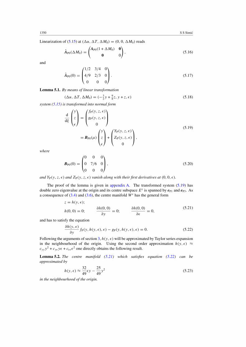
Figure 4. Bifurcation diagram of transcritical bifurcation pattern (5.24).

The bifurcation equation for this problem is obtained by inserting (5.23) into dy/dξ =fP(y, h(y, ε), ε). Expanding the result in Taylor series, the main result of the analysis isobtained.

Theorem 5.2. Bifurcation of equilibrium (y, z, ε) = (0, 0, ε) of (5.19) appears for thebifurcation value of parameter ε = 0 and the corresponding bifurcation equation has the form

dy

dξ= 10

7εy − 20

7y2 + O3 (5.24)

where O3 denotes terms which vanish along with their first and second derivatives with respectto y and ε for (y, ε) = (0, 0).

In order to support this result, a qualitative structure of the bifurcation diagramcorresponding to equation (5.24) is given in figure 4. One may observe that there existsthe trivial solution branch y0(ε) ≡ 0 which corresponds to the upstream equilibrium state. Itis stable for ε < 0 and unstable for ε > 0. On the other hand, the nontrivial solution branchy1(ε) = ε/2 + O(ε2) is transverse to y0 and corresponds to downstream equilibrium. Stabilityproperties of these solutions are indicated in the figure. The flow corresponding to the shockstructure is transverse to both equilibrium branches and corresponds to heteroclinic orbits ofthe dynamical system (5.11).

Note that the stable branch of the bifurcating solution y1(ε) corresponds to physicallyadmissible solutions of Rankine–Hugoniot equations (4.1), in the sense of Lax. However,Lax’s condition has not been exploited at all in stability and bifurcation analysis of this section.In such a way, stability considerations of theorem 5.1 seem to provide an equivalent conditionas the Lax’s one.

Although the local bifurcation analysis may blur a bit the original shock structure problem,it has some useful consequences. In section 7 it will be shown how an approximate solutioncan be constructed from the solution of bifurcation equation (5.24).

6. Stability and bifurcation of equilibrium in extended thermodynamics

In the case of the hyperbolic dissipative model (2.12) travelling shock profile is assumed inthe form U(x, t) = U(ξ), ξ = (x − st)/τ . The PDE system is thus reduced to the systemof ODEs

(−sA0(U) + A(U))

dUdξ

= Q(U), (6.1)

1352 S S Simic

where the small parameter τ disappeared due to scaling of the independent variable. Whenthe profile is considered in the moving frame of reference the problem becomes stationary dueto Galilean invariance, and by introduction of the relative velocity u = v − s, equation (6.1)reduces it to

A(U)dUdξ

= dF(U)

dξ= Q(U). (6.2)

It is accompanied by the following boundary conditions:

U(−∞) =(

u(−∞)

v(−∞)

)=

(u0

h(u0)

);

U(∞) =(

u(∞)

v(∞)

)=

(u1

h(u1)

);

dU(±∞)

dξ= 0

(6.3)

where u0 and u1 are related by Rankine–Hugoniot conditions (2.5). Since these end statesbelong to the equilibrium manifold of (2.12), they are also the stationary points of system (6.2)and the shock structure is again the heteroclinic orbit connecting them.

6.1. Shock structure equations

To obtain dimensionless equations describing the shock structure in extended thermodynamics,the following non-dimensional quantities will be introduced in addition to (5.6)

σ = σ

ρ0RT0; q = q

ρ0RT0c0. (6.4)

By dropping the tildes for convenience, one derives from (2.16) the following system of shockstructure equations:

d

dξ(ρu) = 0;

d

dξ

(5

3ρu2 + ρT − σ

)= 0;

d

dξ

(5

6ρu3 +

5

2ρT u − σu + q

)= 0;

d

dξ

(5

3ρu3 + 3ρT u − 3σu +

6

5q

)= ρT 1−ασ ;

d

dξ

(5

6ρu4 + 4ρT u2 − 5

2σu2 +

16

5qu − 21

10T σ +

3

2ρT 2

)

= −2

3ρT 1−α

(q − 3

2σu

).

(6.5)

In the derivation we used (2.17) and assumption (5.5). The first three equations could beintegrated taking into account the equilibrium values at x = −∞

ρ0 = 1; u0 = M0; T0 = 1; σ0 = 0; q0 = 0, (6.6)

Shock structure in gas dynamics 1353

and used to express ρ, σ and q in terms of u, T and Mach number M0 as parameter

ρ = M0

u;

σ = 5

3M0(u − M0) + M0

T

u− 1;

q = 5

6M0(M

20 − u2) +

5

2M0(1 − T ) +

5

3M0u(u − M0) + M0T − u.

(6.7)

In such a way system (6.5) is reduced to the system of two first-order ODEsdu

dξ= FH(u, T , M0); dT

dξ= GH(u, T , M0), (6.8)

where the right-hand sides have the following form

FH(u, T , M0) = �u

�; GH(u, T , M0) = �T

�, (6.9)

for

� = 1701T 2α + 12150M20 T 2α + 6885M4

0 T 2α − 2988M20 T 1+2α

+ 486M2

0 T 2+2α

u2− 972

M0T1+2α

u− 1620

M30 T 1+2α

u

− 11052M0T2αu − 18420M3

0 T 2αu + 12660M20 T 2αu2;

�u = 4365M20 T 1+α + 7275M4

0 T 1+α − 540M3

0 T 3+α

u3

+ 1485M2

0 T 2+α

u2+ 2475

M40 T 2+α

u2− 945

M0T1+α

u

− 4500M3

0 T 1+α

u− 3075

M50 T 1+α

u− 2340

M30 T 2+α

u

− 4200M30 T 1+αu;

�T = −900M0T1+α − 5500M3

0 T 1+α

− 10000

3M5

0 T 1+α + 1800M30 T 2+α − 270

M30 T 4+α

u4

+ 270M2

0 T 3+α

u3+ 450

M40 T 3+α

u3− 3600

M30 T 2+α

u2

− 1200M5

0 T 2+α

u2+ 2610

M30 T 3+α

u2+ 2250

M20 T 1+α

u

+ 4500M4

0 T 1+α

u+ 1250

M60 T 1+α

u− 810

M20 T 2+α

u

− 1350M4

0 T 2+α

u+ 1750M2

0 T 1+αu

+8750

3M4

0 T 1+αu − 2500

3M3

0 T 1+αu2.

Although these expressions look quite cumbersome, it can be checked that the upstreamequilibrium (u0, T0) = (M0, 1) and the downstream equilibrium (u1, T1), determinedby (5.12), are the stationary points of (6.8): FH(u0, T0, M0) = FH(u1, T1, M0) = 0,GH(u0, T0, M0) = GH(u1, T1, M0) = 0.

1354 S S Simic

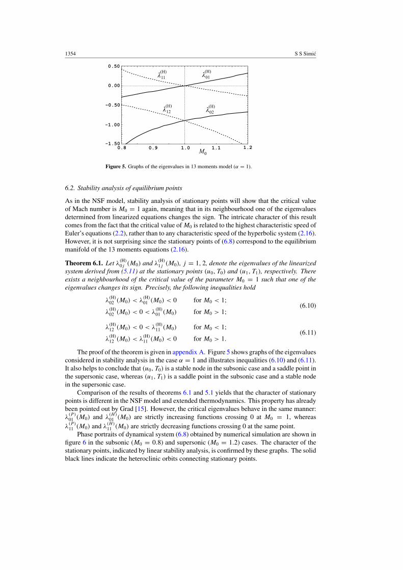
Figure 5. Graphs of the eigenvalues in 13 moments model (α = 1).

6.2. Stability analysis of equilibrium points

As in the NSF model, stability analysis of stationary points will show that the critical valueof Mach number is M0 = 1 again, meaning that in its neighbourhood one of the eigenvaluesdetermined from linearized equations changes the sign. The intricate character of this resultcomes from the fact that the critical value of M0 is related to the highest characteristic speed ofEuler’s equations (2.2), rather than to any characteristic speed of the hyperbolic system (2.16).However, it is not surprising since the stationary points of (6.8) correspond to the equilibriummanifold of the 13 moments equations (2.16).

Theorem 6.1. Let λ(H)0j (M0) and λ

(H)1j (M0), j = 1, 2, denote the eigenvalues of the linearized

system derived from (5.11) at the stationary points (u0, T0) and (u1, T1), respectively. Thereexists a neighbourhood of the critical value of the parameter M0 = 1 such that one of theeigenvalues changes its sign. Precisely, the following inequalities hold

λ(H)02 (M0) < λ

(H)01 (M0) < 0 for M0 < 1;

λ(H)02 (M0) < 0 < λ

(H)01 (M0) for M0 > 1;

(6.10)

λ(H)12 (M0) < 0 < λ

(H)11 (M0) for M0 < 1;

λ(H)12 (M0) < λ

(H)11 (M0) < 0 for M0 > 1.

(6.11)

The proof of the theorem is given in appendix A. Figure 5 shows graphs of the eigenvaluesconsidered in stability analysis in the case α = 1 and illustrates inequalities (6.10) and (6.11).It also helps to conclude that (u0, T0) is a stable node in the subsonic case and a saddle point inthe supersonic case, whereas (u1, T1) is a saddle point in the subsonic case and a stable nodein the supersonic case.

Comparison of the results of theorems 6.1 and 5.1 yields that the character of stationarypoints is different in the NSF model and extended thermodynamics. This property has alreadybeen pointed out by Grad [15]. However, the critical eigenvalues behave in the same manner:λ

(P )01 (M0) and λ

(H)01 (M0) are strictly increasing functions crossing 0 at M0 = 1, whereas

λ(P )11 (M0) and λ

(H)11 (M0) are strictly decreasing functions crossing 0 at the same point.

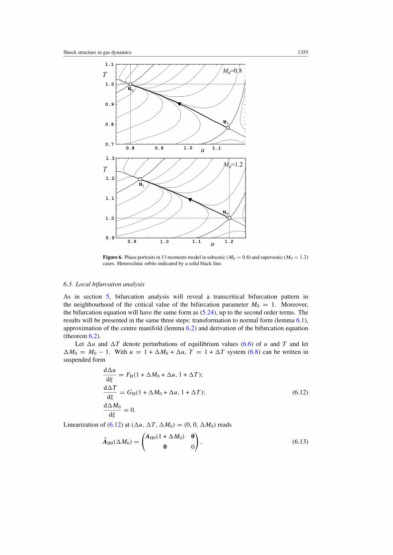
Phase portraits of dynamical system (6.8) obtained by numerical simulation are shown infigure 6 in the subsonic (M0 = 0.8) and supersonic (M0 = 1.2) cases. The character of thestationary points, indicated by linear stability analysis, is confirmed by these graphs. The solidblack lines indicate the heteroclinic orbits connecting stationary points.

Shock structure in gas dynamics 1355

Figure 6. Phase portraits in 13 moments model in subsonic (M0 = 0.8) and supersonic (M0 = 1.2)cases. Heteroclinic orbits indicated by a solid black line.

6.3. Local bifurcation analysis

As in section 5, bifurcation analysis will reveal a transcritical bifurcation pattern inthe neighbourhood of the critical value of the bifurcation parameter M0 = 1. Moreover,the bifurcation equation will have the same form as (5.24), up to the second order terms. Theresults will be presented in the same three steps: transformation to normal form (lemma 6.1),approximation of the centre manifold (lemma 6.2) and derivation of the bifurcation equation(theorem 6.2).

Let �u and �T denote perturbations of equilibrium values (6.6) of u and T and let�M0 = M0 − 1. With u = 1 + �M0 + �u, T = 1 + �T system (6.8) can be written insuspended form

d�u

dξ= FH(1 + �M0 + �u, 1 + �T );

d�T

dξ= GH(1 + �M0 + �u, 1 + �T );

d�M0

dξ= 0.

(6.12)

Linearization of (6.12) at (�u, �T, �M0) = (0, 0, �M0) reads

AH0(�M0) =(

AH0(1 + �M0) 0

0 0

), (6.13)

1356 S S Simic

and

AH0(0) =

−4/13 −6/13 0

−46/117 −23/39 0

0 0 0

. (6.14)

Lemma 6.1. By means of linear transformation

(�u, �T, �M0) = (− 32y + 18

23z, y + z, ε) (6.15)

system (6.12) is transformed into normal form

d

dξ

y

z

ε

=

fH(y, z, ε)

gH(y, z, ε)

0

= BH0(ε)

y

z

ε

+

YH(y, z, ε)

ZH(y, z, ε)

0

,

(6.16)

where

BH0(0) =

0 0 0

0 −35/39 0

0 0 0

, (6.17)

and YH(y, z, ε) and ZH(y, z, ε) are at least of the second order in y and z.

The proof of the lemma is given in appendix A. Linearization of (6.16) has double zeroeigenvalue at the origin and its centre subspace Ec is spanned by eH1 and eH3. Consequently,centre manifold W c has the same general form (5.21) as in the NSF model and has to satisfythe equation

∂h(y, ε)

∂yfH(y, h(y, ε), ε) − gH(y, h(y, ε), ε) = 0. (6.18)

Following the arguments of section 3, h(y, ε) will be approximated by a Taylor seriesexpansion in the neighbourhood of the origin. Using second order approximation h(y, ε) ≈cyyy

2 + cyεyε + cεεε2 one directly obtains the following result.

Lemma 6.2. Centre manifold z = h(y, ε) which satisfies equation (6.18) can beapproximated by

h(y, ε) ≈ 184245εy − 115

196y2 (6.19)

in the neighbourhood of the origin.

The bifurcation equation for this problem is obtained by inserting (6.19) into dy/dξ =fH(y, h(y, ε), ε). Taylor series expansion leads to the main result of the analysis.

Theorem 6.2. Bifurcation of equilibrium (y, z, ε) = (0, 0, ε) of (6.16) appears for thebifurcation value of parameter ε = 0 and the corresponding bifurcation equation has theform

dy

dξ= 10

7εy − 20

7y2 + O3 (6.20)

where O3 denotes terms which vanish along with their first and second derivatives with respectto y and ε for (y, ε) = (0, 0).

Shock structure in gas dynamics 1357

As was pointed out at the beginning of the section, the bifurcation equation (6.20) for theshock structure problem of the hyperbolic dissipative model has the same form as (5.24) forthe parabolic model and the qualitative structure of the bifurcation diagram is completely thesame. In such a way, the stable branch of the bifurcating solution y1(ε) again corresponds tosolutions of Rankine–Hugoniot equations (4.1) which are physically admissible in the senseof Lax, and stability considerations of theorem 6.1 play an equivalent role in the dissipativesystem as Lax’s condition play in Euler’s model.

A brief resume is in order, concerned with the results of the last two sections. It wasshown, by direct calculation, that two mathematically different dissipative continuum modelsof gas dynamics have two common features in the context of stability and bifurcation analysisof equilibrium states:

(i) the upstream equilibrium state ‘loses’ its stability when the shock speed crosses thecritical value—the highest characteristic speed (speed of sound) of the equilibrium system;actually, one of the eigenvalues changes its sign in the neighbourhood of M0 = 1;

(ii) the downstream equilibrium state can be regarded as a bifurcating solution and thebifurcation equation reveals a transcritical bifurcation pattern.

Since Lax’s condition has not been exploited in this analysis, it was claimed that the stabilityresults of theorems 5.1 and 6.1 provide an equivalent selection rule, at least in these cases,which could be directly applied to dissipative models.

A natural question may be posed about possible generalizations. At this moment itcould only be conjectured that these results are valid for general parabolic and hyperbolicdissipative models under certain assumptions, explicitly or implicitly stated in this study.These assumptions are the following:

(i) the shock structure problem is analysed for the shock waves which correspond to thehighest characteristic speeds of the equilibrium system; these characteristic speeds areassumed to be genuinely nonlinear;

(ii) dissipative continuum models, either parabolic or hyperbolic, are reduced to theequilibrium one when dissipation is neglected;

(iii) dissipative models considered in this study are compatible with appropriate companionbalance laws, i.e. entropy inequalities with convex entropy (this is how the closure problemis resolved in extended thermodynamics [22]);

(iv) the hyperbolic dissipative model can be reduced to a parabolic one through asymptoticexpansion akin to the Chapman–Enskog one.

Rigorous study of the stability criterion conjecture has yet to be done. If successful, it willalso remove possible redundancy of the above-mentioned assumptions.

7. Further application of bifurcation analysis

In the absence of general results, capability of stability and bifurcation analysis for furtherapplication can be tested on other systems. It will be shown in this section that analysisyields the same results in more involved models as long as they can be reduced to the sameequilibrium system of Euler’s equations. Particular examples of the 14 and 21 momentsequations of extended thermodynamics will be analysed. A comment will also be given aboutthe linear stability analysis in the neighbourhood of the other critical values of the bifurcationparameter. An interesting possibility for construction of approximate solutions, based uponthe solution of the bifurcation equation in the neighbourhood of the critical point, will also beshown. Discussion will be closed by indication of the benefits of stability analysis in numericalcalculation of shock structure.

1358 S S Simic

7.1. Extended thermodynamics with 14 and 21 fields

In addition to nonequilibrium fields of stress σ and heat flux q, extended thermodynamics with14 fields introduce another variable �—the nonequilibrium part of the fourth moment of thedistribution function [17]. This results in additional balance law which have to be adjoined to(2.16). Using (6.7) the sock structure equations can be reduced to a set of three ODEs, withu, T and � as unknown fields.

By applying the same procedure of stability and bifurcation analysis as in sections 5 and 6,analogous results are obtained. In particular, there exists a neighbourhood of the critical valueof the parameter M0 = 1 such that one of the eigenvalues changes sign

λ(14)03 (M0) < λ

(14)02 (M0) < λ

(14)01 (M0) < 0 for M0 < 1;

λ(14)03 (M0) < λ

(14)02 (M0) < 0 < λ

(14)01 (M0) for M0 > 1;

(7.1)

λ(14)13 (M0) < λ

(14)12 (M0) < 0 < λ

(14)11 (M0) for M0 < 1;

λ(14)13 (M0) < λ

(14)12 (M0) < λ

(14)11 (M0) < 0 for M0 > 1.

(7.2)

To be precise,

λ(14)01 (1) = 0; dλ

(14)01 (1)

dM0= 10

7;

λ(14)11 (1) = 0; dλ

(14)11 (1)

dM0= −10

7;

(7.3)

The suspended system of equations in normal form, obtained via linear transformation(�u, �T, ��, �M0) → (y, z1, z2, ε), has two-dimensional centre manifold approximately,while the bifurcation equation has the same form as (5.24) and (6.20) as in the NSF and 13moments case.

The 21 moments equations do not provide any substantially new contribution whatsoever(for the model consult [22]). Although the order of the shock structure ODE system is greaterby one, a single eigenvalue again plays a distinguished role leading to the same bifurcationpattern. Therefore, even in more involved problems stability and bifurcation analysis supportsour conjecture about two common properties of dissipative models, given at the end of previoussection, as long as the full system of governing equations has the Euler’s system (2.2) as anequilibrium system.

A note has to be added about the stability analysis. In procedures applied in this study, theorder of the original shock structure system has always been immediately reduced by meansof conservation laws (for example, see equation (6.7) derived from the first three equations of(6.5)). As a consequence, all the eigenvalues were real and different from zero except in thecritical case M0 = 1. What would have happened if this reduction had not been done? In thiscase there will appear multiple zero eigenvalue whose algebraic multiplicity is equal to thenumber of conservation laws. However, this fact does not affect the structure and behaviourof other eigenvalues and the main conclusions of stability analysis will remain the same.

7.2. Other critical values of the bifurcation parameter

The main issue of this study was stability and bifurcation analysis of the shock structureproblem. It naturally arises in the neighbourhood of the critical value of the shock speed whichcorresponds to the highest genuinely nonlinear characteristic speed of the equilibrium system.However, there remains an open question about solution behaviour in the neighbourhood ofother critical values of the shock speed corresponding to genuinely nonlinear characteristic

Shock structure in gas dynamics 1359

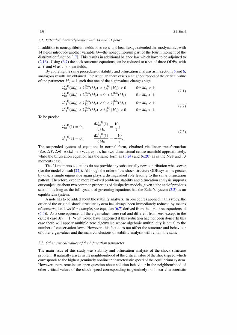
Figure 7. Eigenvalues in the neighbourhood of upstream singular points (7.4).

speeds of the hyperbolic dissipative systems. This problem will be outlined for the 13 momentsmodel (6.8).

Having in mind the structure of equations (6.9) which describe the shock profile, one mayask, when will the right-hand sides become singular, i.e. � = 0. By simple calculation it canbe shown that the singularity condition is satisfied for

M0 = ±0.6297; M0 = ±1.6503. (7.4)

These solutions correspond to characteristic speeds (2.18) of the 13 moments model (2.16).Weiss [30] analysed singular points in detail in the shock structure problem for extendedthermodynamic models and showed that the continuous shock structure ceases to exist whenM0 becomes greater than the highest critical value. This important fact was pointed out byGrad [15] in the case of the 13 moments equations. A general result of this kind, valid forhyperbolic systems of balance laws with convex extension, has been proven by Boillat andRuggeri [3].

Our analysis will be restricted to calculation of the eigenvalues of the linearized systemat the equilibrium state in the neighbourhood of the critical values (7.4). Let us recallthat λ

(H)01 (M0) and λ

(H)11 (M0) change the sign in the neighbourhood of M0 = 1. For the

upstream equilibrium (figure 7), λ(H)01 (M0) is monotonically increasing in the neighbourhood

of M0 = 0.6297, while λ(H)02 (M0) is singular at the same point, having vertical asymptotes. On

the other hand, λ(H)01 (M0) becomes singular at M0 = 1.6503 with vertical asymptotes, while

λ(H)02 (M0) is monotonically increasing in its neighbourhood.

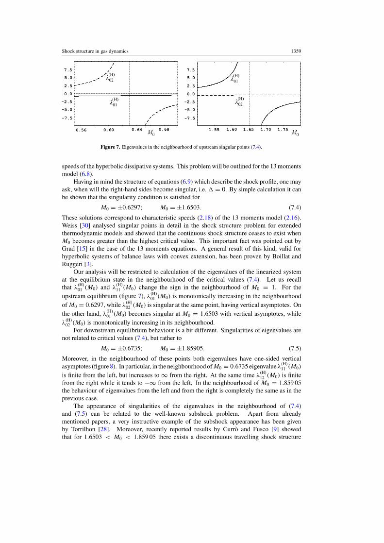
For downstream equilibrium behaviour is a bit different. Singularities of eigenvalues arenot related to critical values (7.4), but rather to

M0 = ±0.6735; M0 = ±1.85905. (7.5)

Moreover, in the neighbourhood of these points both eigenvalues have one-sided verticalasymptotes (figure 8). In particular, in the neighbourhood of M0 = 0.6735 eigenvalue λ

(H)11 (M0)

is finite from the left, but increases to ∞ from the right. At the same time λ(H)12 (M0) is finite

from the right while it tends to −∞ from the left. In the neighbourhood of M0 = 1.859 05the behaviour of eigenvalues from the left and from the right is completely the same as in theprevious case.

The appearance of singularities of the eigenvalues in the neighbourhood of (7.4)and (7.5) can be related to the well-known subshock problem. Apart from alreadymentioned papers, a very instructive example of the subshock appearance has been givenby Torrilhon [28]. Moreover, recently reported results by Curro and Fusco [9] showedthat for 1.6503 < M0 < 1.859 05 there exists a discontinuous travelling shock structure

1360 S S Simic

Figure 8. Eigenvalues in the neighbourhood of downstream singular points (7.5).

with a single jump discontinuity. It is shown to be a consequence of the fact thatequilibrium states in phase space lie on different sides of the so-called singular barrier. WhenM0 > 1.859 05 a discontinuous shock structure is observed with two jump discontinuities.These discontinuities were governed by Rankine–Hugoniot equations for the differential partof the full hyperbolic system of 13 moments equations. A possible way out of this problem hasbeen given by Au, Torrilhon and Weiss [1] through higher order moment systems of extendedthermodynamics. Although some particular conclusions could be drawn from this analysis,a careful study of the singularities is needed in order to reveal all the implications of theirexistence.

7.3. Approximate solutions for very weak shocks

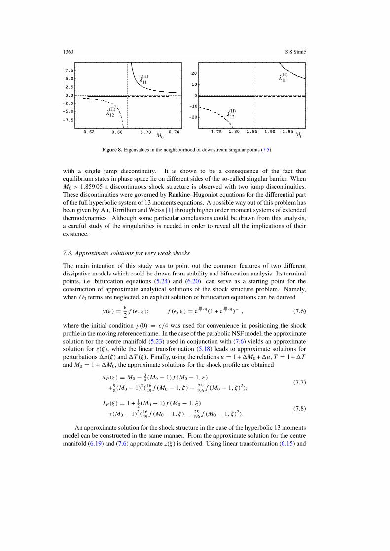
The main intention of this study was to point out the common features of two differentdissipative models which could be drawn from stability and bifurcation analysis. Its terminalpoints, i.e. bifurcation equations (5.24) and (6.20), can serve as a starting point for theconstruction of approximate analytical solutions of the shock structure problem. Namely,when O3 terms are neglected, an explicit solution of bifurcation equations can be derived

y(ξ) = ε

2f (ε, ξ); f (ε, ξ) = e

107 εξ (1 + e

107 εξ )−1, (7.6)

where the initial condition y(0) = ε/4 was used for convenience in positioning the shockprofile in the moving reference frame. In the case of the parabolic NSF model, the approximatesolution for the centre manifold (5.23) used in conjunction with (7.6) yields an approximatesolution for z(ξ), while the linear transformation (5.18) leads to approximate solutions forperturbations �u(ξ) and �T (ξ). Finally, using the relations u = 1 + �M0 + �u, T = 1 + �T

and M0 = 1 + �M0, the approximate solutions for the shock profile are obtained

uP (ξ) = M0 − 34 (M0 − 1)f (M0 − 1, ξ)

+ 98 (M0 − 1)2( 16

49f (M0 − 1, ξ) − 25196f (M0 − 1, ξ)2); (7.7)

TP (ξ) = 1 + 12 (M0 − 1)f (M0 − 1, ξ)

+(M0 − 1)2( 1649f (M0 − 1, ξ) − 25

196f (M0 − 1, ξ)2).(7.8)

An approximate solution for the shock structure in the case of the hyperbolic 13 momentsmodel can be constructed in the same manner. From the approximate solution for the centremanifold (6.19) and (7.6) approximate z(ξ) is derived. Using linear transformation (6.15) and

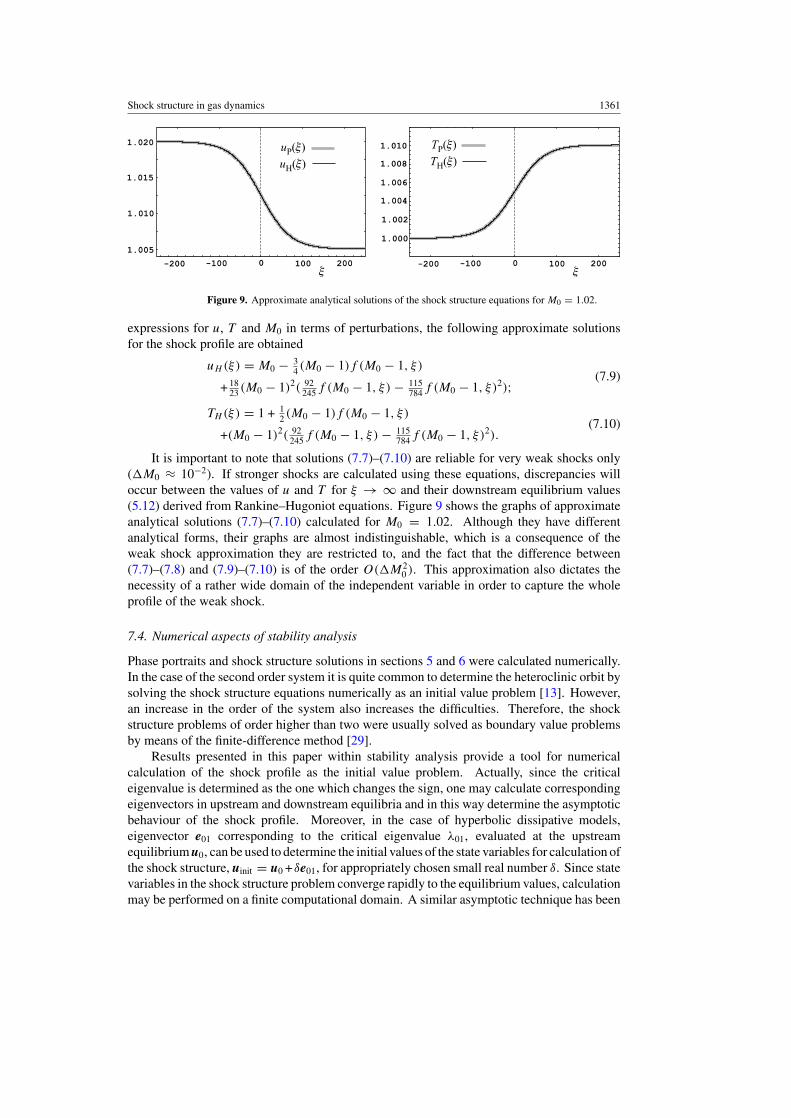
Shock structure in gas dynamics 1361

Figure 9. Approximate analytical solutions of the shock structure equations for M0 = 1.02.

expressions for u, T and M0 in terms of perturbations, the following approximate solutionsfor the shock profile are obtained

uH (ξ) = M0 − 34 (M0 − 1)f (M0 − 1, ξ)

+ 1823 (M0 − 1)2( 92

245f (M0 − 1, ξ) − 115784f (M0 − 1, ξ)2); (7.9)

TH (ξ) = 1 + 12 (M0 − 1)f (M0 − 1, ξ)

+(M0 − 1)2( 92245f (M0 − 1, ξ) − 115

784f (M0 − 1, ξ)2).(7.10)

It is important to note that solutions (7.7)–(7.10) are reliable for very weak shocks only(�M0 ≈ 10−2). If stronger shocks are calculated using these equations, discrepancies willoccur between the values of u and T for ξ → ∞ and their downstream equilibrium values(5.12) derived from Rankine–Hugoniot equations. Figure 9 shows the graphs of approximateanalytical solutions (7.7)–(7.10) calculated for M0 = 1.02. Although they have differentanalytical forms, their graphs are almost indistinguishable, which is a consequence of theweak shock approximation they are restricted to, and the fact that the difference between(7.7)–(7.8) and (7.9)–(7.10) is of the order O(�M2

0 ). This approximation also dictates thenecessity of a rather wide domain of the independent variable in order to capture the wholeprofile of the weak shock.

7.4. Numerical aspects of stability analysis

Phase portraits and shock structure solutions in sections 5 and 6 were calculated numerically.In the case of the second order system it is quite common to determine the heteroclinic orbit bysolving the shock structure equations numerically as an initial value problem [13]. However,an increase in the order of the system also increases the difficulties. Therefore, the shockstructure problems of order higher than two were usually solved as boundary value problemsby means of the finite-difference method [29].

Results presented in this paper within stability analysis provide a tool for numericalcalculation of the shock profile as the initial value problem. Actually, since the criticaleigenvalue is determined as the one which changes the sign, one may calculate correspondingeigenvectors in upstream and downstream equilibria and in this way determine the asymptoticbehaviour of the shock profile. Moreover, in the case of hyperbolic dissipative models,eigenvector e01 corresponding to the critical eigenvalue λ01, evaluated at the upstreamequilibrium u0, can be used to determine the initial values of the state variables for calculation ofthe shock structure, uinit = u0 +δe01, for appropriately chosen small real number δ. Since statevariables in the shock structure problem converge rapidly to the equilibrium values, calculationmay be performed on a finite computational domain. A similar asymptotic technique has been

1362 S S Simic

devised by Beyn [6] in the boundary value problem of heteroclinic orbits and its truncationfrom an infinite domain to a finite one. However, these optimistic ideas have to be carefullytested. Weiss [30] claimed that the appearance of regular singular points within the profilemay prevent simple calculation of the shock profile using the initial value procedure. Detailedanalysis of numerical aspects is beyond the scope of this study and will be the topic ofprospective work.

8. Conclusions

The shock structure problem in continuum theory of fluids is a well-known and challengingproblem, both physically and mathematically. In the latter context two different types ofmathematical models appeared with the intention of describing this phenomenon in theappropriate way, i.e. taking into account dissipative mechanisms. The first type—parabolicsystems of PDEs—is usually identified with, but not exhausted by, the NSF model whichintroduces dissipation in the classical Euler’s equations of gas dynamics through diffusiveterms, related to viscosity and heat conduction. Another group of models falls into the categoryof hyperbolic systems of balance laws with dissipative source terms. The 13 moments model,obtained in the context of extended thermodynamics, has been taken as a paradigmatic one forthis group. This paper tends to impart the common ground of these models through stabilityand bifurcation analysis of equilibrium states.

The analysis was based upon the ODE system of the shock structure equations derivedfrom the original PDE model using travelling wave ansatz. In such a way the equilibriumstates became stationary points of the dynamical system describing the shock structure. Thefirst important result of the study is obtained by means of linear stability analysis. It wasdemonstrated that in both models there always exists a distinguished eigenvalue which changesthe sign in the neighbourhood of the critical value of the parameter M0 = 1, correspondingto the highest characteristic speed of the equilibrium system—Euler’s model. Since Lax’sadmissibility condition has not been used in the analysis, stability results stated in theorems 5.1and 6.1 can be used as selection rules for admissible shock structures in dissipative models.Bifurcation analysis gave the second result by revealing the common transcritical bifurcationpattern which appears in both models (theorems 5.2 and 6.2).

This study opened some new questions indicated in section 7. First, it is naturalto seek for possible generalizations of the results presented here. For what concernsparabolic models, it seems that a positive answer could be given in a straightforwardmanner, whereas for hyperbolic systems of balance laws thorough study has yet to beperformed. Second, a rigorous singularity analysis in hyperbolic models, related to othercritical values of the parameter, is another open question. Finally, the computational aspectof stability analysis and its consequences in analytical and numerical calculation of theshock profiles has to be carefully studied. These are possible lines of investigation infuture work.

Acknowledgments

This work was supported by the Ministry of Science of the Republic of Serbia within the project‘Contemporary problems of mechanics of deformable bodies’ (Project No 144019). The authoris indebted to Professor Tommaso Ruggeri (University of Bologna, Italy) and Professor IngoMuller (Technical University Berlin, Germany) for numerous fruitful discussions and usefulcomments and suggestions during the preparation of this paper.

Shock structure in gas dynamics 1363

Appendix A. Proofs of theorems and lemmas

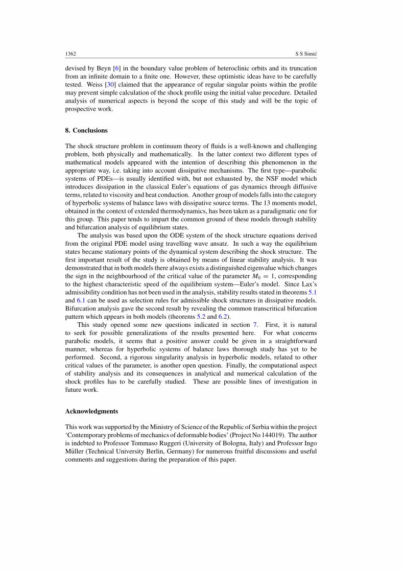
Proof of theorem 5.1. The proof will be given for the upstream equilibrium state first and thenfor the downstream equilibrium. The Jacobian matrix for system (5.11) at (u0, T0) = (M0, 1)

reads

AP0(M0) =(

14 (5M0 − 3

M0) 3

4

49

23M0

), (A.1)

while corresponding eigenvalues are

λ(P)01 (M0) = D0−

24M0; λ

(P)02 (M0) = D0+

24M0;

D0∓ = −9 + 23M20 ∓

√81 + 66M2

0 + 49M40 ,

(A.2)

and the following holds

λ(P)01 (1) = 0; λ

(P)02 (1) = 7

6 ;dλ

(P)01 (1)

dM0= 10

7.

(A.3)

By the continuity argument it follows that there is a neighbourhood of M0 = 1 in whichλ

(P)01 (M0) < 0 for M0 < 1 and λ

(P)01 (M0) > 0 for M0 > 1, while λ

(P)02 (M0) > 0 in either case

which proves (5.13).The Jacobian matrix at (u1, T1) given by (5.12) reads

AP1(M0) = 16α

(14 − 3

M20

+ 5M20

)−α

×

9M0 − 5M30

2(3 + M20 )

3M20

3 + M20

1

9

(−1 + 5M20

) 2

3M0

,

(A.4)

while the corresponding eigenvalues are

λ(P)11 (M0) =

16α

(14 − 3

M20

+ 5M20

)−α

12(3 + M20 )

D1−

λ(P)12 (M0) =

16α

(14 − 3

M20

+ 5M20

)−α

12(3 + M20 )

D1+;

D1∓ = 39 − 11M20 ∓

√81 + 102M2

0 + 601M40

(A.5)

and the following holds

λ(P)11 (1) = 0; λ

(P)12 (1) = 7

6;

dλ(P)11 (1)

dM0= −10

7.

(A.6)

Again, the continuity argument helps to conclude that there is a neighbourhood of M0 = 1 inwhich λ

(P)11 (M0) > 0 for M0 < 1 and λ

(P)11 (M0) < 0 for M0 > 1, while λ

(P)12 (M0) > 0 in either

case, which proves (5.14).

1364 S S Simic

Note that at (u0, T0) eigenvalues depend only on M0 and not on α, while at (u1, T1) theyalso depend on the type of gas through α. However, their values as well as behaviour of thecritical eigenvalue at M0 = 1 are independent of α.

Proof of lemma 5.1. By straightforward calculation from (5.17) one can obtain theeigenvalues of AP0(0), (λP1, λP2, λP3) = (0, 7/6, 0), and the corresponding set of eigenvectors(eP1, eP2, eP3) which actually determines the transformation matrix

TP = (eP1, eP2, eP3) =

−3/2 9/8 0

1 1 0

0 0 1

. (A.7)

Linear transformation (5.18) is obtained through (�u, �T, �M0)T = TP · (y, z, ε)T, where

superposed T stands for transposition. The right-hand side of (5.19) is determined as(fP(y, z, ε), gP(y, z, ε), 0)T = T−1

P · (FP(y, z, ε), GP(y, z, ε), 0)T, where FP and GP areobtained from FP and GP when (�u, �T, �M0) is substituted by means of (5.18). The linearpart BP0(ε) can be obtained either as a Jacobian of the right-hand side of the complete systemevaluated at (y, z, ε) = (0, 0, ε), or through BP0(ε) = T−1

P · AP0(ε) · TP. For the sake ofbrevity complete expressions for fP and gP will be omitted since they can be obtained in astraightforward way.

Proof of theorem 6.1. The Jacobian matrix for system (6.8) at (u0, T0) = (M0, 1) reads

AH0(M0) = 1

27 − 78M20 + 25M4

0

×

−9 + 42M20 − 25M4

0

M03(3 + M2

0 )

54 − 162M20 + 200M4

0

9M20

−18 + 114M20 − 50M4

0

3M0

,

(A.8)

while corresponding eigenvalues are

λ(H)01 (M0) = 5D0−

6M0(27 − 78M20 + 25M4

0 );

λ(H)02 (M0) = 5D0+

6M0(27 − 78M20 + 25M4

0 );

D0∓ = −9 + 48M20 − 25M4

0

∓√

81 − 216M20 + 234M4

0 + 72M60 + 25M8

0 ,

(A.9)

and the following holds

λ(H)01 (1) = 0; λ

(H)02 (1) = −35

39;

dλ(H)01 (1)

dM0= 10

7.

(A.10)

By the continuity argument it follows that there is a neighbourhood of M0 = 1 in whichλ

(H)01 (M0) < 0 for M0 < 1 and λ

(H)01 (M0) > 0 for M0 > 1, while λ

(H)02 (M0) < 0 in either case

which proves (6.10).

Shock structure in gas dynamics 1365

The Jacobian matrix at (u1, T1) determined by (5.12) reads

AH1(M0) = 16α

(1 − 5M20 )

(14 − 3

M20

+ 5M20

)−α

(3 + M20 )(243 − 606M2

0 + 155M40 )

(A.11)

×(

4M0(45 − 66M20 + 5M4

0 ) −96M40

118 (585 − 402M2

0 + 185M40 ) 1

3 (405 − 738M20 − 35M4

0 )

).

Corresponding eigenvalues λ(H)11 (M0) and λ

(H)12 (M0) can be evaluated explicitly, but have a

rather cumbersome form. Nevertheless, the following results can be derived:

λ(H)11 (1) = 0; λ

(H)12 (1) = −35

39;

dλ(H)11 (1)

dM0= −10

7,

(A.12)

which, due to continuity, lead to a conclusion that there is a neighbourhood of M0 = 1 inwhich λ

(H)11 (M0) > 0 for M0 < 1 and λ

(H)11 (M0) < 0 for M0 > 1, while λ

(H)12 (M0) < 0 in either

case, which proves (6.11).

Proof of lemma 6.1. From (6.14) the eigenvalues of AH0(0) are calculated, (λH1, λH2, λH3) =(0, −35/39, 0), along with the corresponding set of eigenvectors (eH1, eH2, eH3) whichdetermines the transformation matrix

TH = (eH1, eH2, eH3) =

−3/2 18/23 0

1 1 0

0 0 1

. (A.13)

Linear transformation (6.15) is determined by (�u, �T, �M0)T = TH · (y, z, ε)T.

The right-hand side of (6.16) is determined as (fH(y, z, ε), gH(y, z, ε), 0)T = T−1H ·

(FH(y, z, ε), GH(y, z, ε), 0)T, where FH and GH are obtained from FH and GH when(�u, �T, �M0) is substituted by means of (6.15). The linear part BH0(ε) can be obtained eitheras a Jacobian of the right-hand side of the complete system evaluated at (y, z, ε) = (0, 0, ε),or through BH0(ε) = T−1

H · AH0(ε) · TH. For the sake of brevity complete expressions for fH,gH and BH0(ε) will be omitted.

References

[1] Au J D, Torrilhon M and Weiss W 2001 The shock tube study in extended thermodynamics Phys. Fluids13 2423–32

[2] Azevedo A V, Marchesin D, Plohr B and Zumbrun K 1999 Bifurcation of nonclassical viscous shock profilesfrom the constant state Commun. Math. Phys. 202 267–90

[3] Boillat G and Ruggeri T 1998 On the shock structure problem for hyperbolic system of balance laws and convexentropy Contin. Mech. Thermodyn. 10 285–92

[4] Bose C, Illner R and Ukai S 1998 On shock wave solutions for discrete velocity models of the Boltzmannequation Transport Theory Statist. Phys. 27 35–66

[5] Bernhoff N and Bobylev A 2007 Weak shock waves for the general discrete velocity model of the Boltzmannequation Commun. Math. Sci. 5 815–32

[6] Beyn W-J 1990 The numerical computation of connecting orbits in dynamical systems IMA J. Numer. Anal.10 379–405

[7] Caflisch R E and Nicolaenko B 1982 Shock profile solutions of the Boltzmann equation Commun. Math. Phys.86 161–94

1366 S S Simic

[8] Courant R and Friedrichs K O 1948 Supersonic Flow and Shock Waves (New York: Interscience Publishers)[9] Curro C and Fusco D 2005 Discontinuous travelling wave solutions for a class of dissipative hyperbolic models

Rend. Mat. Acc. Lincei 16 61–71[10] Dafermos C M 2005 Hyperbolic Conservation Laws in Continuum Physics 2nd edn (Berlin: Springer)[11] Farjami Y and Hesaaraki M 1998 Structure of shock waves in planar motion of plasma Nonlinearity 11 797–821[12] Gilbarg D 1951 The existence and limit behavior of the one-dimensional shock layer Am. J. Math. 73 256–74[13] Gilbarg D and Paolucci D 1953 The structure of shock waves in the continuum theory of fluids J. Ration. Mech.

Anal. 2 617–42[14] Grad H 1949 On the kinetic theory of rarefied gases Commun. Pure Appl. Math. 2 331–407[15] Grad H 1952 The profile of a steady planar shock wave Commun. Pure Appl. Math. 5 257–300[16] Guckenheimer J and Holmes P 1986 Nonlinear Oscillations, Dynamical Systems and Bifurcations of Vector

Fields (New York: Springer)[17] Kremer G M 1986 Extended thermodynamics of ideal gases with 14 fields Ann. Inst. H. Poincare Phys. Theor.

45 419–40[18] Lax P D 1957 Hyperbolic systems of conservation laws: II Commun. Pure Appl. Math. 10 537–66[19] Lorin E 2003 Existence of viscous profiles for the compressible Navier–Stokes equations Appl. Anal. 82 645–54[20] Liu T-P 1987 Hyperbolic conservation laws with relaxation Commun. Math. Phys. 108 153–75[21] Majda A and Pego R L 1985 Stable viscosity matrices for systems of conservation laws J. Diff. Eqns 56 229–62[22] Muller I and Ruggeri T 1998 Rational Extended Thermodynamics (New York: Springer)[23] Nicolaenko B and Thurber J K 1975 Weak shock and bifurcating solutions of the non-linear Boltzmann equation

J. Mecanique 14 305–38[24] Perko L 2001 Differential Equations and Dynamical Systems 3rd edn (New York: Springer)[25] Schecter S 1992 Heteroclinic bifurcation theory and Riemann problems Mat. Contemp. 3 165–90[26] Serre D 1999 Systems of Conservation Laws (Cambridge: Cambridge University Press)[27] Simic S S 2008 A note on shock profile in dissipative hyperbolic and parabolic models Publ. Inst. Math. (N.S.)

84 97–107[28] Torrilhon M 2000 Characteristic waves and dissipation in the 13-moment-case Contin. Mech. Thermodyn.

12 289–301[29] Torrilhon M and Struchtrup H 2004 Regularized 13-moment equations: shock structure calculations and

comparison to Burnett models J. Fluid Mech. 513 171–98[30] Weiss W 1995 Continuous shock structure in extended thermodynamics Phys. Rev. E 52 R5760–3[31] Yong W-A and Zumbrun K 2000 Existence of relaxation shock profiles for hyperbolic conservation laws SIAM

J. Appl. Math. 60 1565–75