Shocks – Do SVAR Models Justify Discarding the Technology ... · Shocks – Do SVAR Models Justify Discarding the Technology Shock-Driven Real Business Cycle Hypothesis?† Hyeon-seung

Shocks – Do SVAR Models Justify Discarding the Technology Shock-Driven Real Business Cycle Hypothesis?†

Hyeon-seung Huh David Kim School of Economics School of Economics

Yonsei University University of Sydney Republic of Korea Australia

[email protected] [email protected]

Abstract

___________________________________________________________________________ Recent studies by Gali (1999), Gali and Rabanal (2004) and Francis and Ramey (2005) raise a strong objection to the technology shock-driven real business cycle (RBC) hypothesis on empirical grounds. To further investigate the validity of technology shocks as a driving force of U.S. business cycle fluctuations, we revisit some of the most commonly understood structural vector autoregression (SVAR) models of the empirical business cycle: namely, Gali (1999), Shapiro and Watson (1988), and King, Plosser, Stock and Watson (1991). Unlike previous contributions, we utilize these models to analyze how structural shocks are associated with the variations of output and hours worked at business cycle frequencies. Empirical evidence indicates that, across the models, technology shocks remain as an important source of cyclical movements in output even if all other shocks are combined and used against the technology shocks. Furthermore, in contrast to previous studies, our results show that a positive technology shock does not lead to a decline in hours worked. These results remain robust whether hours worked is assumed to be a difference-stationary or trend-stationary process. Our SVAR-based evidence does not support discarding a technology shock-driven business cycle theory. ___________________________________________________________________________ Keywords: Structural vector autoregressive (SVAR) models, Technology shocks, Demand

shocks, Real business cycle theory. JEL Classification: C32, E32.

† The authors wish to thank Lance Fisher, Gary Hansen, Glenn Otto, and Adrian Pagan for helpful comments, as well as participants at the 2011 Econometric Society Asian Meetings and the 2011 Australasian Macroeconomics Workshop. This work was supported by the National Research Foundation of Korea Grant funded by the Korean Government (NRF-2011-327-B00098). The usual caveats apply.

2

1. Introduction

Is the quest for the dominant driver of economic fluctuations over? Furthermore, should the

technology shock-driven real business cycle (RBC) hypothesis be discarded? The RBC

hypothesis posits that technology or productivity shocks are the dominant source of

fluctuations, propagated through intertemporal substitutions by optimizing households and

firms in response to the shocks. The hypothesis implies that government stabilization policies

could be counter-productive. In contrast, the New Keynesian models emphasize the role of

demand shocks propagated due to the presence of price stickiness and imperfect competition,

hence justifying active demand management through short-run stabilization programs. Thus,

empirical investigation of the main source of business cycle fluctuations is important not only

as a guide for developing a useful positive theory but also because policy implications can

vary substantially, depending on which interpretation is correct.

Following the emergence of the New Keynesian research program, there has been a

considerable debate as to whether the RBC predictions are borne out by data. Many empirical

studies have relied on structural vector autoregression (SVAR) approaches to evaluate the

empirical validity of the RBC hypothesis. Notably, Gali (1999), Gali and Rabanal (2004), and

Francis and Ramey (2005) all reported that, in SVAR models, positive technology shocks

lead to a decline in hours worked, casting serious doubt on the usefulness of RBC theory as a

quantitative theory of economic fluctuations. Typically, these studies use long-run restrictions

to identify shocks with the interpretation of “technology shocks” and compare how the

congruence between the impulse responses from an estimated SVAR model and those of an

RBC model. A key yardstick used to evaluate the RBC hypothesis using an estimated SVAR

model is whether “technology shocks lead to a rise in hours?” in actual data as predicted by

the theory.

However, McGrattan (2004), Christiano et al. (2003), and Chari et al. (2008) all

challenged this rejection of technology-shock driven RBC models based on such an

3

evaluation strategy. Specifically, they argued that the SVAR models used to refute RBC-

based explanations are either misspecified or not appropriately designed to evaluate the

calibrated general equilibrium business cycle theory. In a similar vein, Wang and Wen (2011)

argued that conditional impulse responses generated by SVAR models cannot serve as

grounds to reject the technology shock-driven RBC hypothesis because the dimension of such

a highly stylized model is different from that of an empirical characterization of data.

In this paper, we utilize several SVAR models and present a set of further results that

provide alternative perspectives into the empirical source of fluctuations. Our work is not an

attempt to engage in the methodological debate over the best practice to empirically evaluate

the RBC theory or, more generally, calibrated macroeconomic models. While our SVAR

analysis produces impulse response functions, we do not simply follow what Gali and others

did in their analyses. Instead, we focus on business cycle frequencies and estimate the

contribution of technology vs. demand (and other) shocks by imposing a minimal number of

identifying assumptions. Hence, our work is similar, in spirit, to Cochrane (1994a) in that it

is a quest for which empirical shocks drive business cycle fluctuations. Unlike Cochrane’s

bivariate setting, however, we employ extended models that accommodate various underlying

shocks to allow for different dynamics depending on the nature of the shocks. The results are

used to examine the robustness of empirical findings produced by the existing stream of

SVAR models.

The SVAR models utilized here are taken from Gali (1999), Shapiro and Watson

(1988), and King et al. (1991). These three SVAR models were selcted because they are

among the best understood and the most popular models in empirical business cycle research.

Along with these SVAR models, we use the decomposition of permanent and transitory

components as a key analytical tool, similar to that of Beveridge and Nelson (1981). The

permanent component determines the long-run movements of the variables, while the

transitory component captures the short-run dynamics. Both components can be constructed

4

after estimating structural models in conjunction with identifying restrictions. This allows us

to analyze how the underlying shocks of models are associated with the transitory component

of output, which captures fluctuations at business cycle frequencies. Based on the conditional

correlations of shocks with cyclical output, we examine how different structural shocks have

contributed to postwar U.S. business cycle fluctuations. We also provide detailed findings on

two important issues. First, we shed light on whether the importance of technology shocks is

sensitive to whether hours worked is specified to be difference-stationary or trend-stationary,

as RBC proponents such as Christiano et al. (2004) have argued. The other issue concerns

the empirical findings that a positive technology shock leads to a decline in hours, which Gali

and others have used as evidence against the RBC theory. Overall, this study provides further

and alternative perspectives using the evidence that is clearly at odds with the earlier findings

of Gali and others.

The remainder of this paper is organized as follows. Section 2 outlines the three

SVAR models explored in the paper, and Section 3 presents our empirical strategy for

measuring the relative contribution of structural shocks in accounting for the business cycle

fluctuations of the variables. The results are given in Section 4. Section 5 offers further

discussion of the results, with particular emphasis on robustness, and revisits the issue raised

by Gali concerning the relationship between technology shocks and hours worked. Section 6

summarizes the key results of the paper and concludes the paper.

2. SVAR models

This section reviews the three SVAR models and explains how they are used in our

investigation.

2.1. Gali (1999)

5

Gali investigated whether technology shocks could explain postwar U.S. business cycles

using an SVAR model, to conclude that the technology shocks have a limited ability to

explain the business cycle. He adopted two models: (i) a bivariate SVAR model comprising

labor productivity (x) (defined as output less hours worked) and hours worked (n), i.e. with

the vector , ,t tx n and (ii) a five-variable SVAR model with the vector of variables

, , , , t t t t t t tx n m p R p p , where, in addition to labor productivity and hours worked,

real money balances (nominal money, m, less the price level, p), real interest rates (nominal

interest rates, R, minus the rate of inflation, Δp), and the inflation rate (Δp) enter the system.1

In the current paper, we consider only the latter model as the bivariate model does not make a

distinction between non-technology supply shocks and demand shocks. The five-variable

SVAR model assumes that there are five structural shocks: technology shocks ( 1tv ), labor

supply shocks ( 2tv ), and three demand-side shocks ( 3tv , 4tv , and 5tv ).

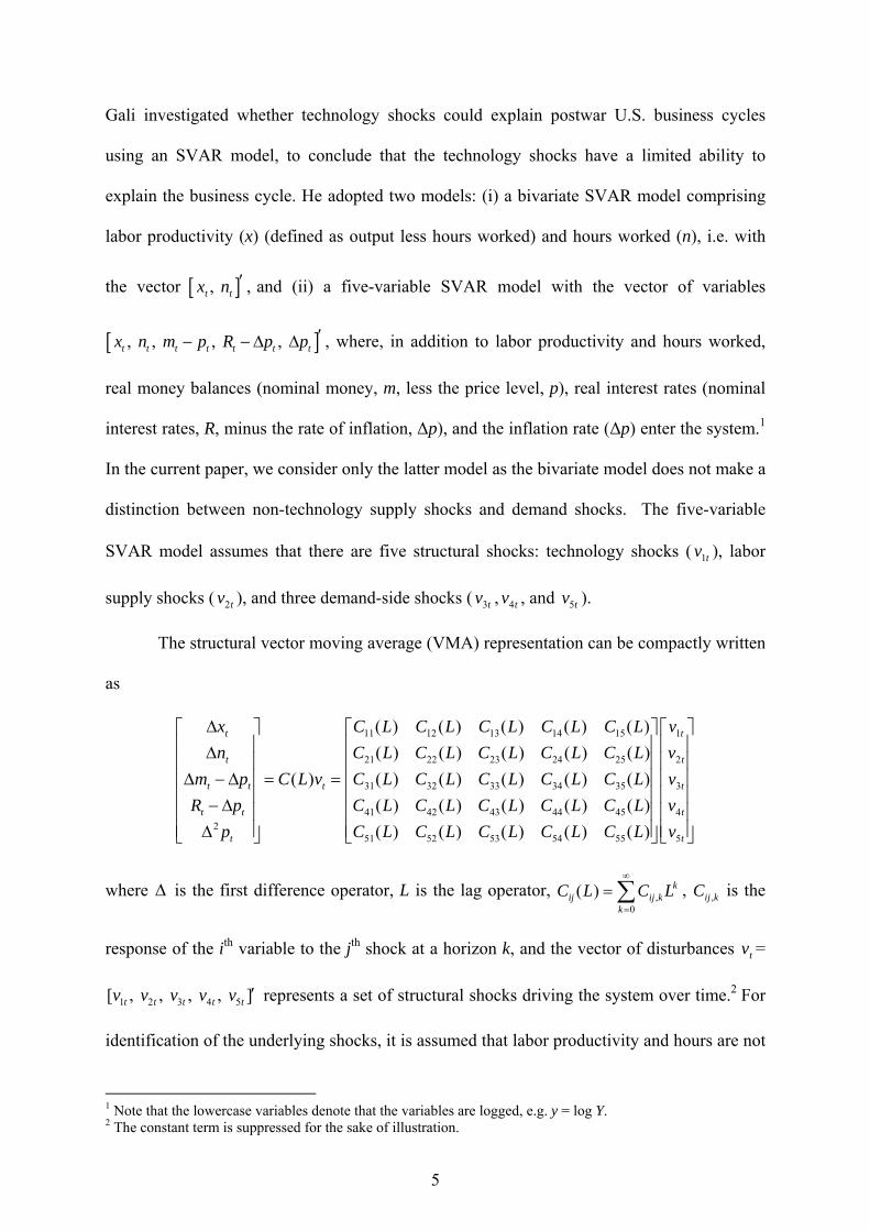
The structural vector moving average (VMA) representation can be compactly written

as

11 12 13 14 15

21 22 23 24 25

31 32 33 34 35

41 42 43 44 452

51 52 53 54 55

( ) ( ) ( ) ( ) ( )

( ) ( ) ( ) ( ) ( )

( ) ( ) ( ) ( ) ( ) ( )

( ) ( ) ( ) ( ) ( )

( ) ( ) ( ) ( ) ( )

t

t

t t t

t t

t

x C L C L C L C L C L

n C L C L C L C L C L

m p C L v C L C L C L C L C L

R p C L C L C L C L C L

p C L C L C L C L C L

1

2

3

4

5

t

t

t

t

t

v

v

v

v

v

where is the first difference operator, L is the lag operator, ,0

( ) kij ij k

k

C L C L

, ,ij kC is the

response of the ith variable to the jth shock at a horizon k, and the vector of disturbances tv =

1 2 3 4 5[ , , , , ]t t t t tv v v v v represents a set of structural shocks driving the system over time.2 For

identification of the underlying shocks, it is assumed that labor productivity and hours are not

1 Note that the lowercase variables denote that the variables are logged, e.g. y = log Y. 2 The constant term is suppressed for the sake of illustration.

6

affected by the three demand shocks, 3tv , 4tv , and 5tv , in the long run. The implied

restrictions can be imposed by assuming that 1 2(1) (1) 0j jC C for j = 3, 4 and 5, where

,0

(1)ij ij kk

C C

measures the long-run response of the ith variable to the jth shock. This

distinguishes the technology and labor supply shocks from the demand shocks. The two

supply shocks are identified individually on the assumption that the labor supply shock has

no long-run effect on labor productivity by setting 12(1) 0C . The three demand shocks are

not disentangled individually, and their combined effects are used. As output is obtained

through the relationship that t t ty x n , it is affected by the two supply shocks at all

horizons, while none of the demand shocks has long-run effects.

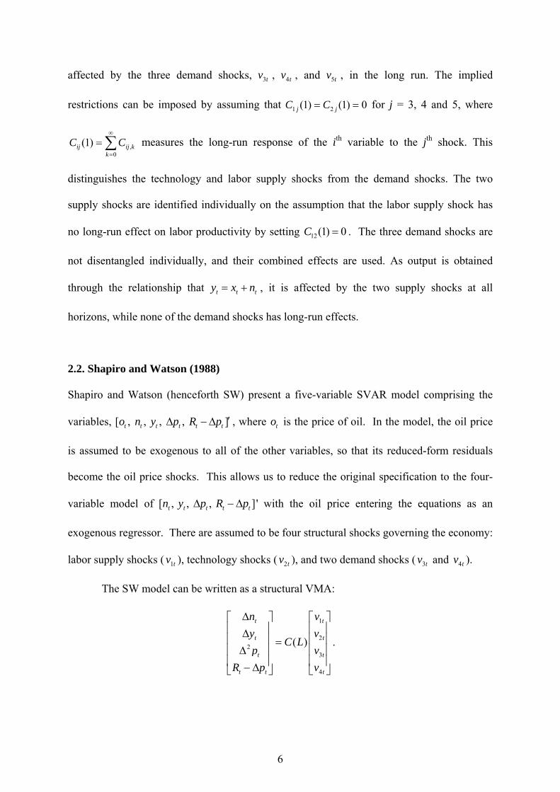
2.2. Shapiro and Watson (1988)

Shapiro and Watson (henceforth SW) present a five-variable SVAR model comprising the

variables, [ , , , , ]t t t t t to n y p R p , where to is the price of oil. In the model, the oil price

is assumed to be exogenous to all of the other variables, so that its reduced-form residuals

become the oil price shocks. This allows us to reduce the original specification to the four-

variable model of [ , , , ]'t t t t tn y p R p with the oil price entering the equations as an

exogenous regressor. There are assumed to be four structural shocks governing the economy:

labor supply shocks ( 1tv ), technology shocks ( 2tv ), and two demand shocks ( 3tv and 4tv ).

The SW model can be written as a structural VMA:

1

22

3

4

( )

t t

t t

t t

t t t

n v

y vC L

p v

R p v

.

7

The labor supply shock is identified on the assumption that it is the only shock that has a

long-run effect on hours. This is equivalent to assuming that 12 13 14(1) (1) (1) 0C C C . The

technology shock is identified using the long-run output neutrality so that the two demand

shocks do not have long-run effects on output. This can be imposed by setting that

23 24(1) (1) 0C C . Again, the demand shocks are not identified individually, and their

combined effects are considered instead.

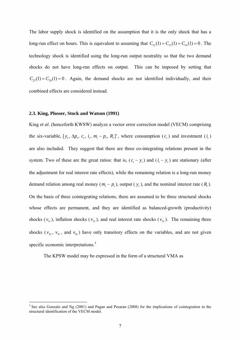
2.3. King, Plosser, Stock and Watson (1991)

King et al. (henceforth KWSW) analyze a vector error correction model (VECM) comprising

the six-variable, [ , , , , , ]'t t t t t t ty p c i m p R , where consumption ( tc ) and investment ( ti )

are also included. They suggest that there are three co-integrating relations present in the

system. Two of these are the great ratios: that is, ( t tc y ) and ( t ti y ) are stationary (after

the adjustment for real interest rate effects), while the remaining relation is a long-run money

demand relation among real money ( t tm p ), output ( ty ), and the nominal interest rate ( tR ).

On the basis of three cointegrating relations, there are assumed to be three structural shocks

whose effects are permanent, and they are identified as balanced-growth (productivity)

shocks ( 1tv ), inflation shocks ( 2tv ), and real interest rate shocks ( 3tv ). The remaining three

shocks ( 4tv , 5tv , and 6tv ) have only transitory effects on the variables, and are not given

specific economic interpretations.3

The KPSW model may be expressed in the form of a structural VMA as

3 See also Gonzalo and Ng (2001) and Pagan and Pesaran (2008) for the implications of cointegration in the structural identification of the VECM model.

8

12

2

3

4

5

6

( )

t t

t t

t t

t t

t t t

t t

y v

p v

c vC L

i v

m p v

R v

The productivity (technology) shock is identified under the assumption that neither the

inflation shock nor the real interest rate shock has a long-run effect on output by setting that

12 13(1) (1) 0C C . 4 The shocks to inflation and the real interest rate are individually

identified by assuming that the real interest rate shock does not have a long-run effect on the

inflation, which implies that 23(1) 0C . These three restrictions are sufficient for exact

identification of the permanent shocks in the model, as the presence of three transitory shocks

implies that all of the elements in the last three columns of C(1) are zero, i.e. (1) 0ijC for

i=1, 2, ,6 and j=4, 5, and 6.

Unlike the Gali and SW models, KPSW allow for investment dynamics to be

expressed within the system. Cogley and Nason (1995) showed that investment dynamics

plays a central role through adjustment lags or costs in accounting for the propagation

mechanism. McGrattan (2004) eloquently argued that technology shocks typically influence

the business cycle through investment, rather than hours. Her point casts doubt on the

premise of sticky-price models of the business cycle model because such models, including

the one studied by Gali, dispense with the role of investment in propagating technology

shocks. Fama (1992) also presented evidence that the hump-shaped response of output is

largely due to the multiplier effect of variations in investment. A recent work by Fisher

(2006) further strengthened the case for the importance of investment and the role of

investment-specific technology shocks.

4 We use the terms productivity and technology interchangeably unless stated otherwise.

9

3. Measuring the contribution of structural shocks

Let Z be a (k×1) vector of variables consisting of k1 non-stationary variables and k2 stationary

variables, i.e. 1 2, t t tZ X X . The structural VMA representation can be compactly

expressed as

( )t tZ L v (1)

where vt represents a vector of structural shocks, and the lag polynomial matrix ( )L tracks

the response of Z to the structural shocks. For expositional convenience, assume that output

in differenced form, Δy, is the first variable in the vector Z. This allows the following

decomposition in a manner analogous to Beveridge and Nelson (1981):

( ) ( ) ( )p ct y t yp t yc ty L v L v L v (2)

where ptv is a vector of shocks that have permanent effects on output, e.g., technology shocks,

and ctv is a vector of shocks that exert only transitory effects, e.g., IS and LM shocks.

Equation (2) can be further decomposed as

(1) ( ) ( ) (1) ( ) ( )p c p p ct yp yp t yc t yp t yp t yc ty L v L v v L v L v (3)

where ( )yp L = ( ) (1)yp ypL , (1)yp captures the effects of ptv on the long-term trend of

output, and ( )yp L measures the effects of ptv on the short-run dynamics of output. For

instance, technology shocks affect long-run output, which is reflected in (1)yp , and also

cause business cycles through changes in capital investment and adjustment costs or lags in

labor input, that is captured by ( ).yp L Equation (3) can be transformed in levels as

0 0 0

(1) ( ) ( )t t t

p c p p ct t t yp t yp t yc t

t t ty y y v L v L v

(4)

In (4), the cyclical component of output corresponds to

0 0( ) ( )

t tc p ct yp t yc t

t ty L v L v

. As it comprises the components separately driven by

10

permanent shocks and transitory demand shocks, we are able to examine which shock is

mainly responsible for fluctuations in output at business cycle frequencies. This may provide

a better way of defining determinants underlying business cycles than the typical tool of

impulse responses and variance decompositions. For technology shocks, the effect on output

is captured by ( )yp L , which can be decomposed into the effect on the short-run dynamics

( )yp L as well as the effect on the long-term trend (1)yp .

Using the decomposition outlined above, we calculate the conditional correlations of

different shocks with the cyclical component of output. To take a five-variable model as an

example, let be the correlation coefficient between cyclical output cty and the first shock

in the model, say, technology shock 1tv . Then, the coefficient ,2345v captures the correlation

of cty with all other shocks combined, indexed 2 to 5 combined, e.g., the composite non-

technology shocks. The conditional correlation quantifies the extent to which each structural

shock is associated with output fluctuations at business cycle frequencies. In addition, by

squaring the correlation coefficients, we can analyze the contribution of the shocks to

accounting for the variance of cty . To see this, rewrite c

ty in (4) as

01 1 02 2 03 3 04 4 05 5

11 1 1 12 2 1 13 3 1 14 4 1 15 5 1

21 1 2 22 2 2 23 3 2 24 4 2 25 5 2

ct t t t t t

t t t t t

t t t t t

y a v a v a v a v a v

a v a v a v a v a v

a v a v a v a v a v

Then, the conditional correlation of cty with the ith shock itv can be obtained as

2 20

, 52 20

1

( , )c i iv i t it

i ii

aCorr y v

a

Where 2i is the variance of the shock itv . Squaring the coefficient of the correlation yields

,1v

11

2 222 0

, , 52 20

1

( , )c i iv i t i t

i ii

aCorr y v

a

The denominator represents the variance of cty explained by all shocks in time t and the

numerator measures the contribution of the ith shock itv .

4. Empirical results

4.1. Impulse responses and historical decompositions

The Gali, SW, and KPSW models in Section 2 are estimated using the same data series, lag

lengths, and starting dates as those used in the original contributions.5 This paper, however,

extends the sample period for all models to end in 2008:Q4.6 We first present the results from

impulse responses and historical decompositions. For the former, we examine how a variable

responds to the structural shocks and check whether these responses are consistent with the

theory. For the latter, we assess the ability of structural shocks to explain the stochastic

movement in a variable over time. At the outset it should be remembered that demand shocks

in the Gali and SW models, and transitory shocks in the KPSW model were not individually

identified (see Section 2). As such, the responses of the variables to these shocks are not

reported in the impulse response analysis, while the historical decomposition analysis reports

their combined contribution to tracking the stochastic movements of the variables. It should

be noted that hours worked is assumed to be a difference-stationary process. In the next

section, we will examine how the results differ when hours worked is assumed to be a trend-

stationary process.

(i) Gali SVAR

5 The number of lags is 4, 6, and 8, and the starting date is 1959:Q1, 1951:Q1, and 1954:Q1 for the Gali, SW, and KPSW models, respectively. 6 This effectively excludes the full effect of the recent financial crisis as an outlier.

12

Figure 1.1 depicts the responses of labor productivity, output and hours in levels to the two

supply-side shocks identified, that is, technology (TN) and labor supply (LS) shocks. Also

reported around each response is the one standard error confidence interval generated by

1,000 bootstrap replications. All of the responses are not different from those presented by

Gali. A positive technology shock raises labor productivity and output permanently, while

hours show a significant decline at short time horizons. As Gali forcefully argues, this finding

is apparently evidence against the RBC theory, which predicts pro-cyclical labor hours in

response to technology shocks. A positive labor supply shock increases hours and output

permanently, and the effect on labor productivity converges to zero by the identifying

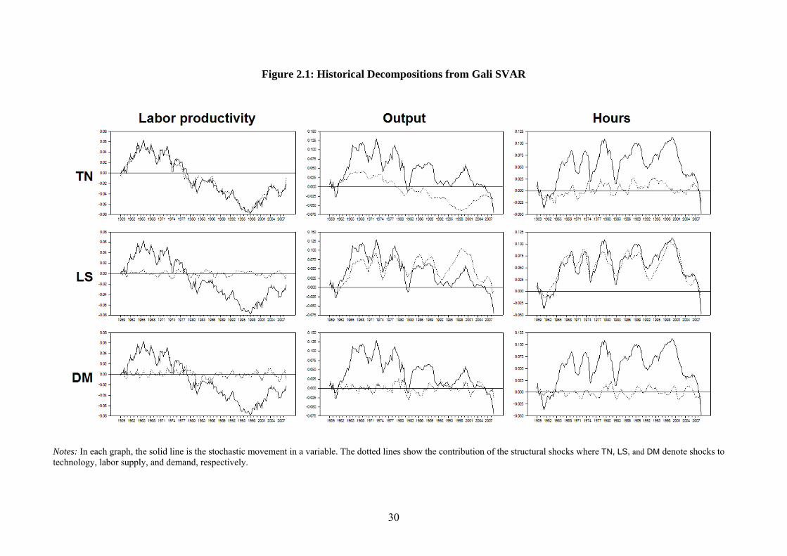
assumption. Figure 2.1 shows the historical decompositions of the key variables. Technology

shocks explain most of the variation in labor productivity, while the variation of hours is

mostly accounted for by labor supply shocks. Interestingly, the result shows that the labor

supply shock is also the main determinant of the movements in output. None of the

technology or demand shocks plays any significant role. We will discuss these results

subsequently in detail.

(ii) Shapiro and Watson SVAR

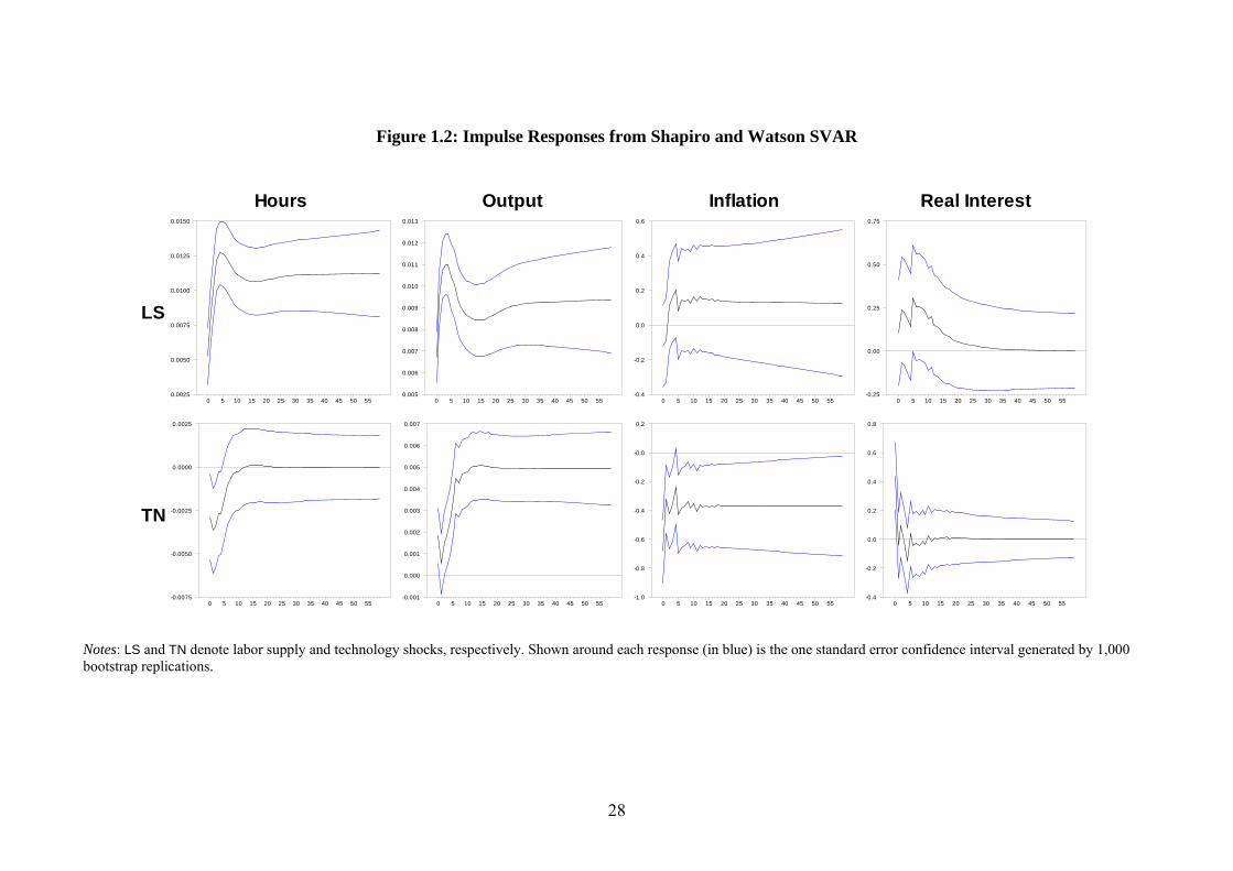
Figure 1.2 shows the responses of the variables to technology and labor supply shocks

estimated from the SW model. Overall, output and hours respond in a very similar manner to

the Gali model. The level of hours falls in response to a positive technology shock before

converging to zero by the identifying restriction. Positive shocks to labor supply and

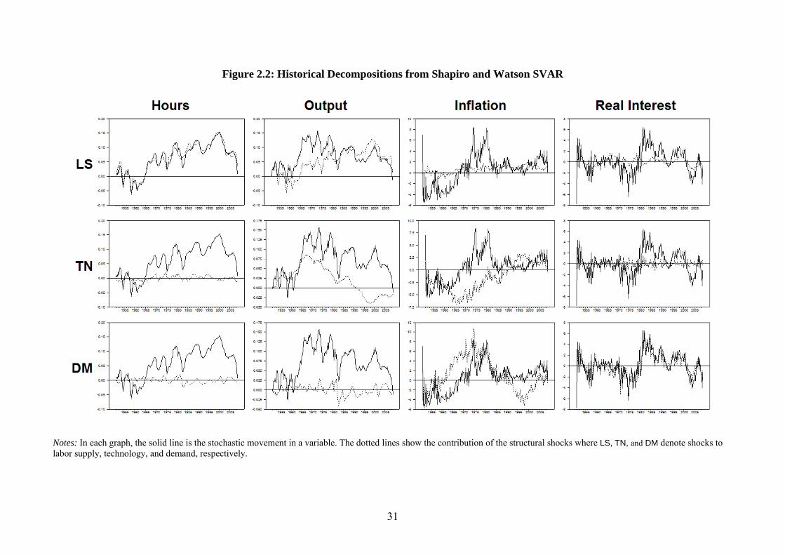
technology increase output permanently. The historical decomposition yields similar results,

as displayed in Figure 2.2. The labor supply shock is the main factor in explaining the

stochastic movements in hours and output, while technology and demand shocks contribute

little to the movements in output.

13

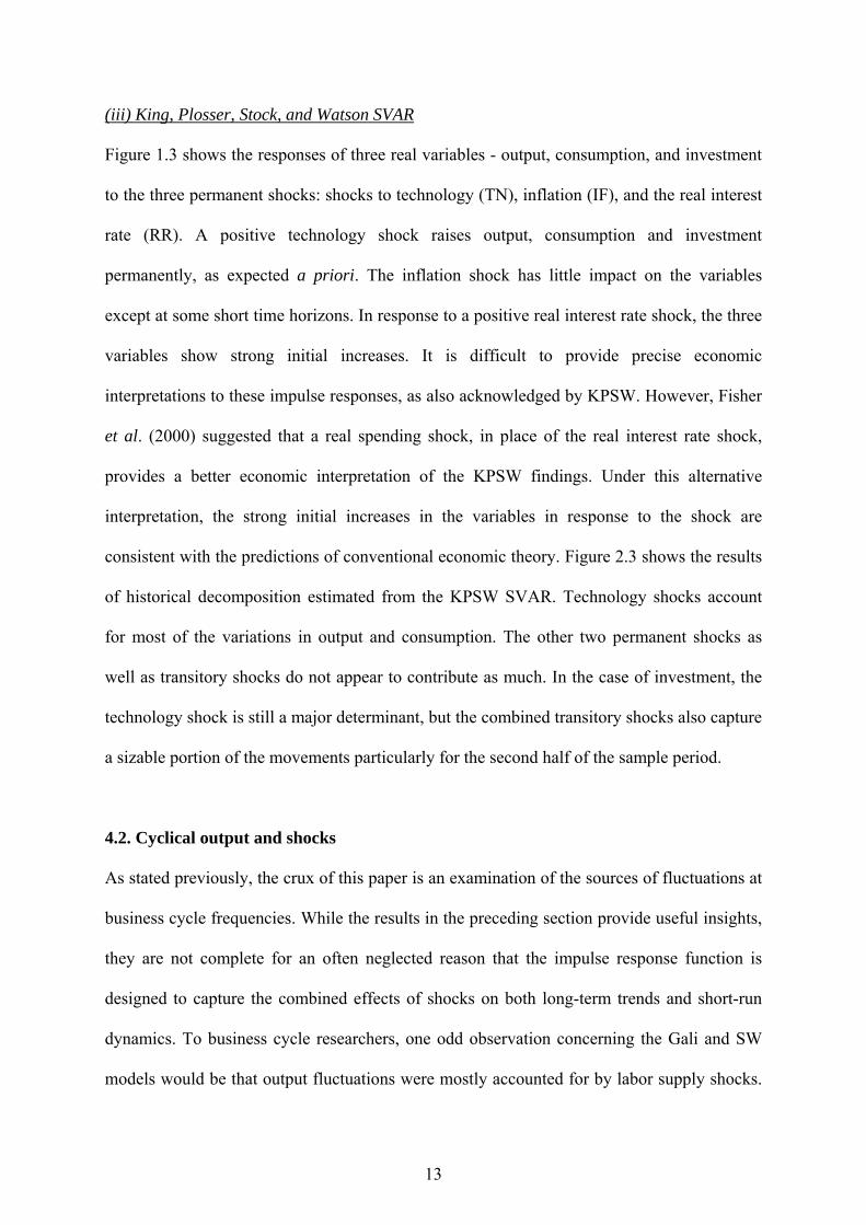
(iii) King, Plosser, Stock, and Watson SVAR

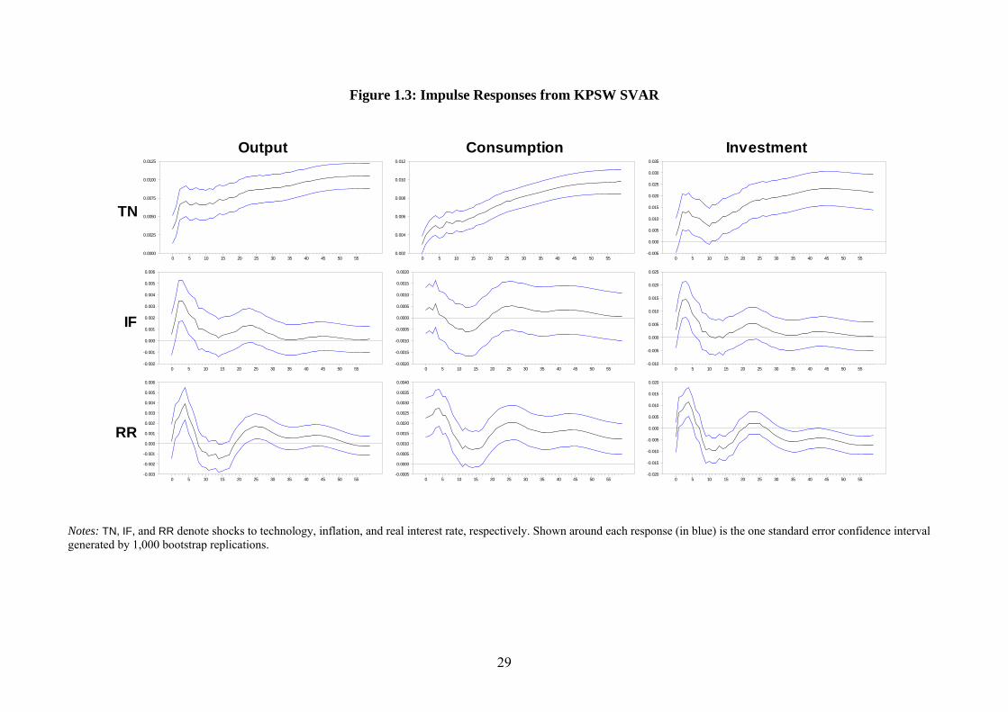
Figure 1.3 shows the responses of three real variables - output, consumption, and investment

to the three permanent shocks: shocks to technology (TN), inflation (IF), and the real interest

rate (RR). A positive technology shock raises output, consumption and investment

permanently, as expected a priori. The inflation shock has little impact on the variables

except at some short time horizons. In response to a positive real interest rate shock, the three

variables show strong initial increases. It is difficult to provide precise economic

interpretations to these impulse responses, as also acknowledged by KPSW. However, Fisher

et al. (2000) suggested that a real spending shock, in place of the real interest rate shock,

provides a better economic interpretation of the KPSW findings. Under this alternative

interpretation, the strong initial increases in the variables in response to the shock are

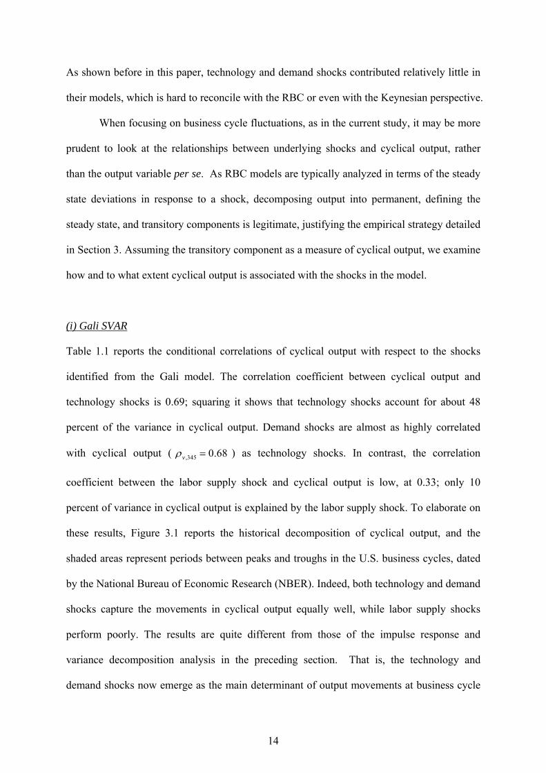
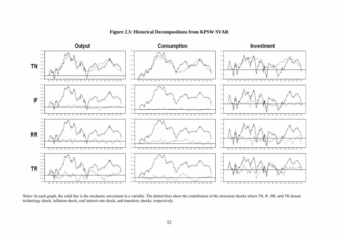
consistent with the predictions of conventional economic theory. Figure 2.3 shows the results

of historical decomposition estimated from the KPSW SVAR. Technology shocks account

for most of the variations in output and consumption. The other two permanent shocks as

well as transitory shocks do not appear to contribute as much. In the case of investment, the

technology shock is still a major determinant, but the combined transitory shocks also capture

a sizable portion of the movements particularly for the second half of the sample period.

4.2. Cyclical output and shocks

As stated previously, the crux of this paper is an examination of the sources of fluctuations at

business cycle frequencies. While the results in the preceding section provide useful insights,

they are not complete for an often neglected reason that the impulse response function is

designed to capture the combined effects of shocks on both long-term trends and short-run

dynamics. To business cycle researchers, one odd observation concerning the Gali and SW

models would be that output fluctuations were mostly accounted for by labor supply shocks.

14

As shown before in this paper, technology and demand shocks contributed relatively little in

their models, which is hard to reconcile with the RBC or even with the Keynesian perspective.

When focusing on business cycle fluctuations, as in the current study, it may be more

prudent to look at the relationships between underlying shocks and cyclical output, rather

than the output variable per se. As RBC models are typically analyzed in terms of the steady

state deviations in response to a shock, decomposing output into permanent, defining the

steady state, and transitory components is legitimate, justifying the empirical strategy detailed

in Section 3. Assuming the transitory component as a measure of cyclical output, we examine

how and to what extent cyclical output is associated with the shocks in the model.

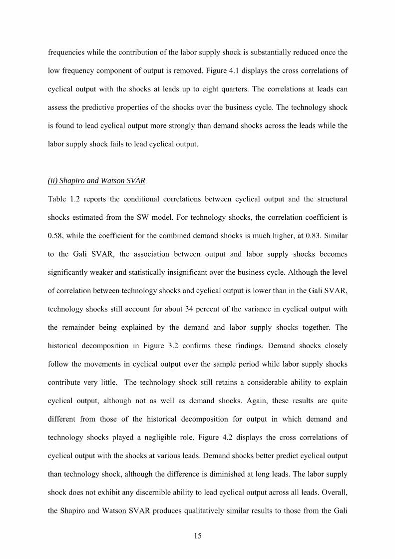
(i) Gali SVAR

Table 1.1 reports the conditional correlations of cyclical output with respect to the shocks

identified from the Gali model. The correlation coefficient between cyclical output and

technology shocks is 0.69; squaring it shows that technology shocks account for about 48

percent of the variance in cyclical output. Demand shocks are almost as highly correlated

with cyclical output ( ,345 0.68v ) as technology shocks. In contrast, the correlation

coefficient between the labor supply shock and cyclical output is low, at 0.33; only 10

percent of variance in cyclical output is explained by the labor supply shock. To elaborate on

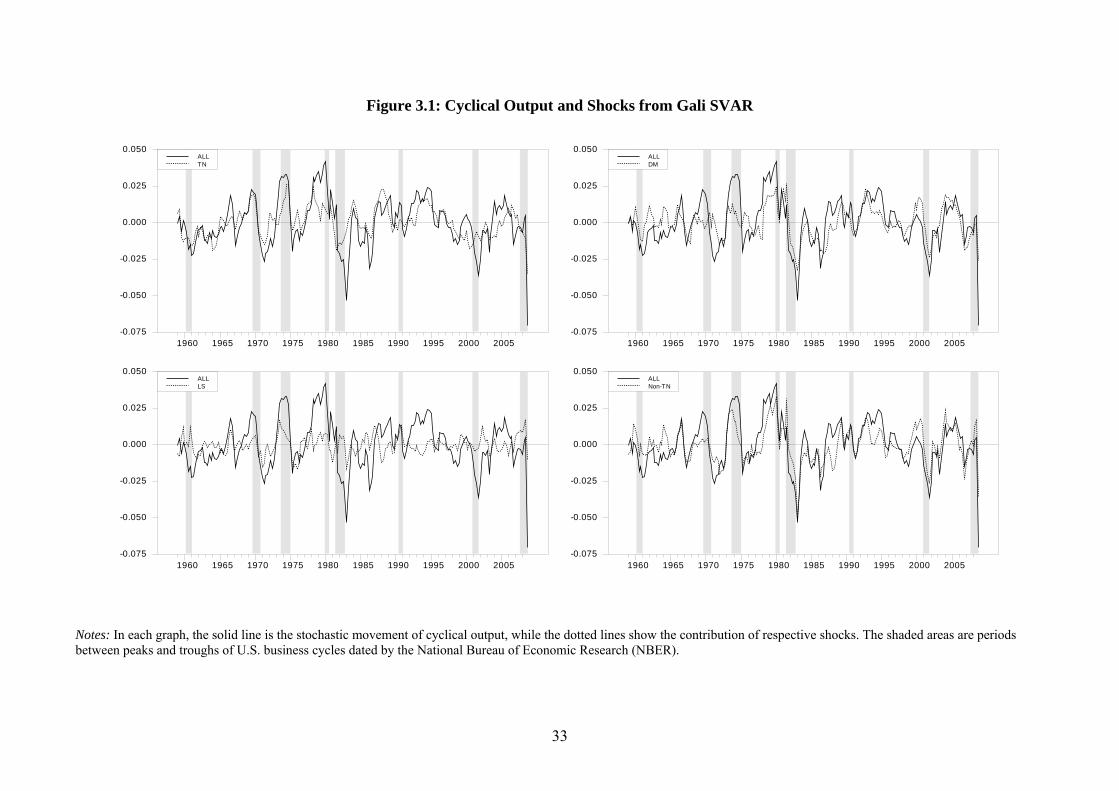
these results, Figure 3.1 reports the historical decomposition of cyclical output, and the

shaded areas represent periods between peaks and troughs in the U.S. business cycles, dated

by the National Bureau of Economic Research (NBER). Indeed, both technology and demand

shocks capture the movements in cyclical output equally well, while labor supply shocks

perform poorly. The results are quite different from those of the impulse response and

variance decomposition analysis in the preceding section. That is, the technology and

demand shocks now emerge as the main determinant of output movements at business cycle

15

frequencies while the contribution of the labor supply shock is substantially reduced once the

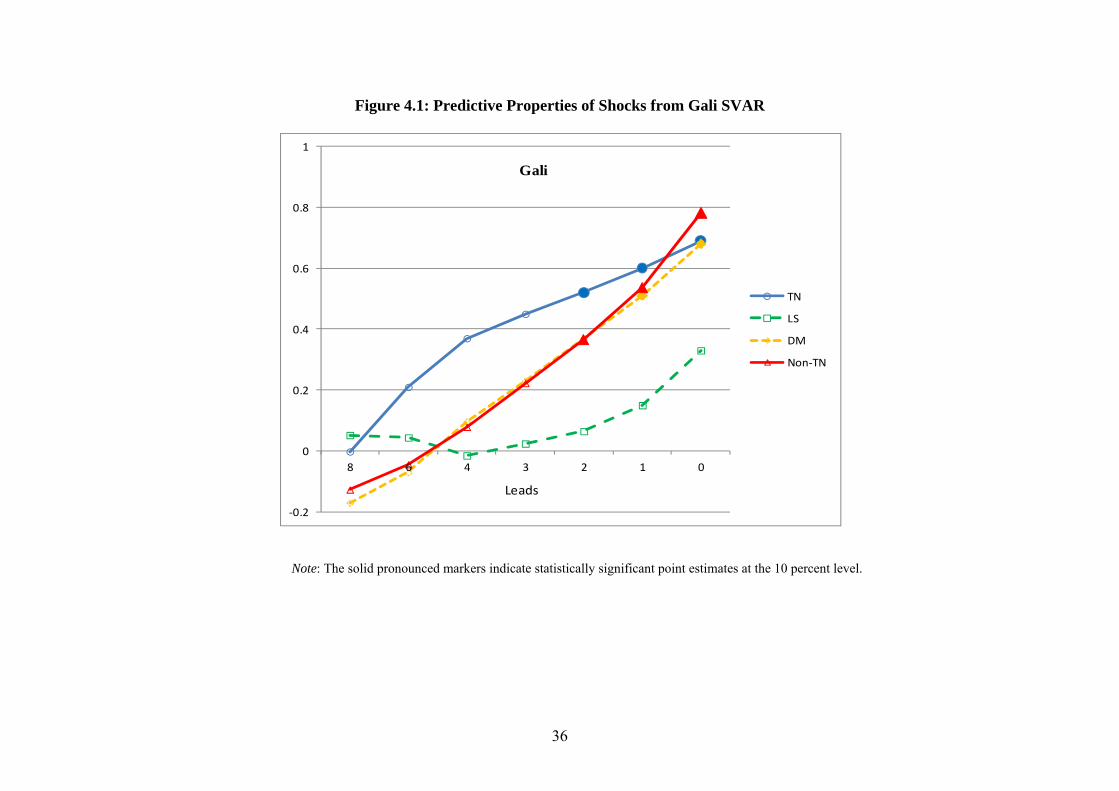
low frequency component of output is removed. Figure 4.1 displays the cross correlations of

cyclical output with the shocks at leads up to eight quarters. The correlations at leads can

assess the predictive properties of the shocks over the business cycle. The technology shock

is found to lead cyclical output more strongly than demand shocks across the leads while the

labor supply shock fails to lead cyclical output.

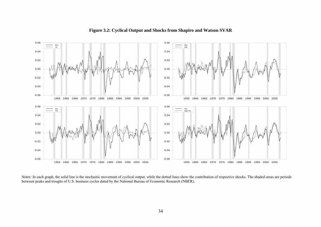
(ii) Shapiro and Watson SVAR

Table 1.2 reports the conditional correlations between cyclical output and the structural

shocks estimated from the SW model. For technology shocks, the correlation coefficient is

0.58, while the coefficient for the combined demand shocks is much higher, at 0.83. Similar

to the Gali SVAR, the association between output and labor supply shocks becomes

significantly weaker and statistically insignificant over the business cycle. Although the level

of correlation between technology shocks and cyclical output is lower than in the Gali SVAR,

technology shocks still account for about 34 percent of the variance in cyclical output with

the remainder being explained by the demand and labor supply shocks together. The

historical decomposition in Figure 3.2 confirms these findings. Demand shocks closely

follow the movements in cyclical output over the sample period while labor supply shocks

contribute very little. The technology shock still retains a considerable ability to explain

cyclical output, although not as well as demand shocks. Again, these results are quite

different from those of the historical decomposition for output in which demand and

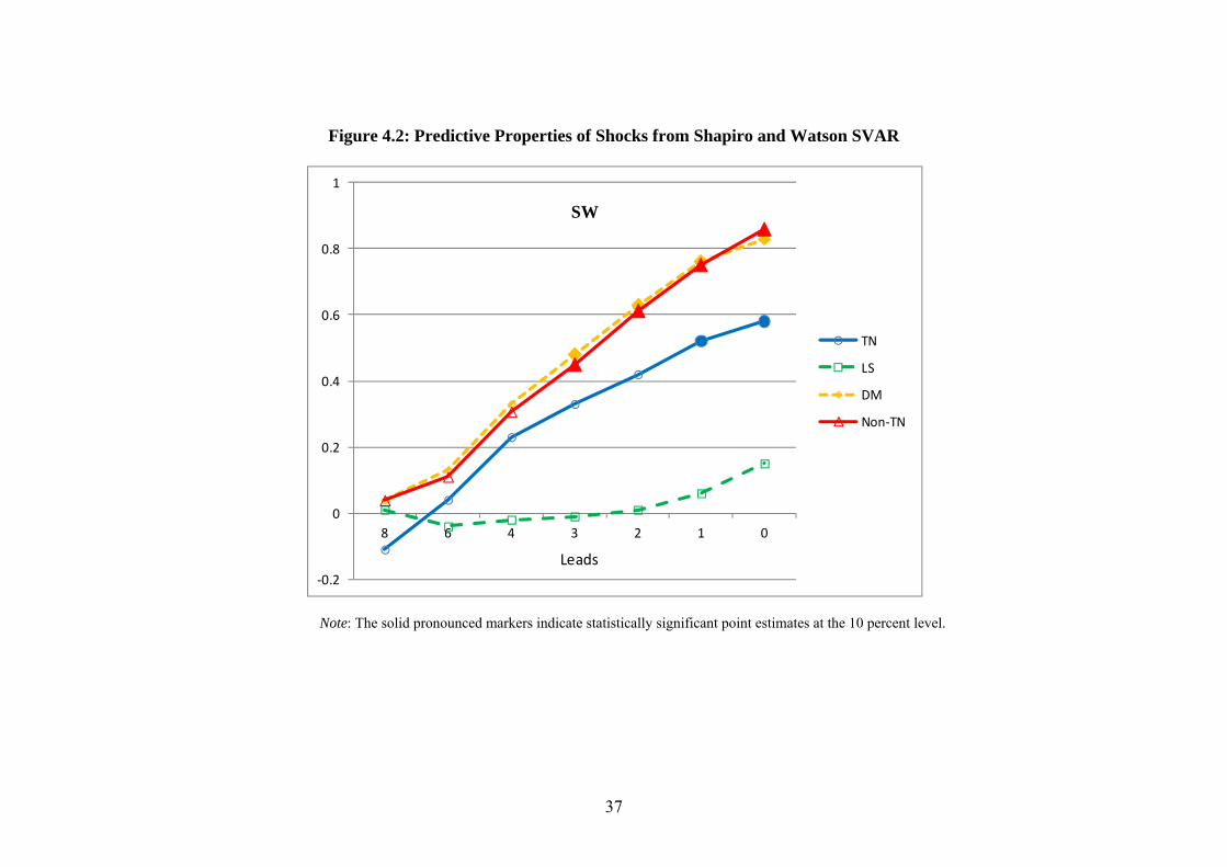
technology shocks played a negligible role. Figure 4.2 displays the cross correlations of

cyclical output with the shocks at various leads. Demand shocks better predict cyclical output

than technology shock, although the difference is diminished at long leads. The labor supply

shock does not exhibit any discernible ability to lead cyclical output across all leads. Overall,

the Shapiro and Watson SVAR produces qualitatively similar results to those from the Gali

16

SVAR. In both models, technology and demand shocks are the main drivers of cyclical

output, while the labor supply shock becomes insignificant.

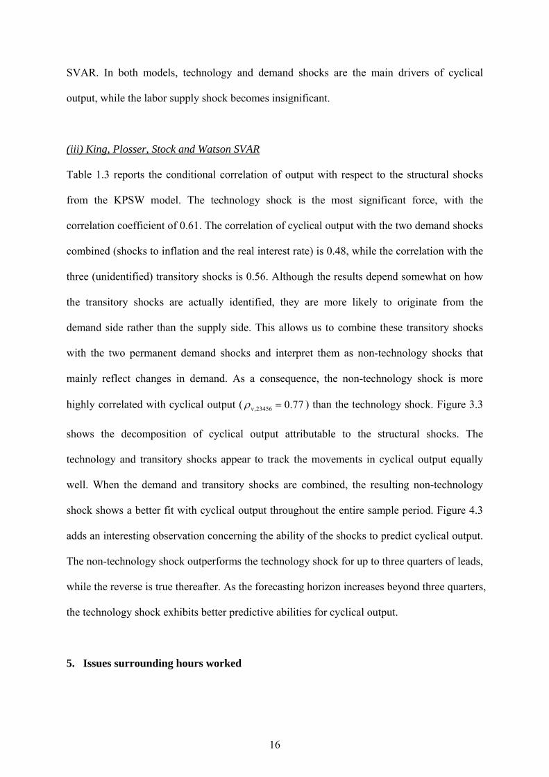
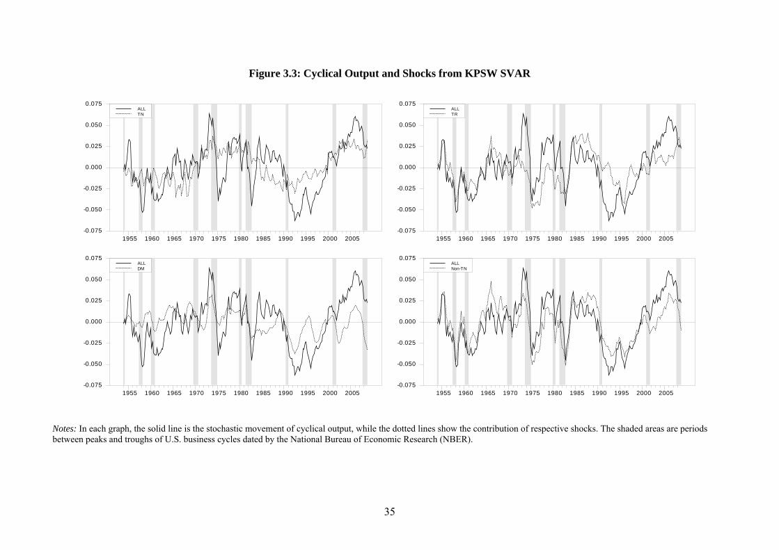
(iii) King, Plosser, Stock and Watson SVAR

Table 1.3 reports the conditional correlation of output with respect to the structural shocks

from the KPSW model. The technology shock is the most significant force, with the

correlation coefficient of 0.61. The correlation of cyclical output with the two demand shocks

combined (shocks to inflation and the real interest rate) is 0.48, while the correlation with the

three (unidentified) transitory shocks is 0.56. Although the results depend somewhat on how

the transitory shocks are actually identified, they are more likely to originate from the

demand side rather than the supply side. This allows us to combine these transitory shocks

with the two permanent demand shocks and interpret them as non-technology shocks that

mainly reflect changes in demand. As a consequence, the non-technology shock is more

highly correlated with cyclical output ( ,23456 0.77v ) than the technology shock. Figure 3.3

shows the decomposition of cyclical output attributable to the structural shocks. The

technology and transitory shocks appear to track the movements in cyclical output equally

well. When the demand and transitory shocks are combined, the resulting non-technology

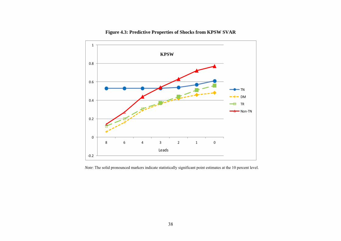
shock shows a better fit with cyclical output throughout the entire sample period. Figure 4.3

adds an interesting observation concerning the ability of the shocks to predict cyclical output.

The non-technology shock outperforms the technology shock for up to three quarters of leads,

while the reverse is true thereafter. As the forecasting horizon increases beyond three quarters,

the technology shock exhibits better predictive abilities for cyclical output.

5. Issues surrounding hours worked

17

In the New Keynesian-RBC debate over the importance of technology shocks, there are two

important issues concerning the empirical characterization of hours worked. The first issue is

the sensitivity of the results to the assumption of whether hours worked is difference-

stationary or trend-stationary. The second issue, related to the first one, is whether a positive

technology shock does, in fact, lead to a decline in hours worked, as argued by Gali (1999).

This section addresses each of these issues with respect to our results from the Gali and SW

models.

5.1. Stationary vs. non-stationary hours worked

Theoretically speaking, hours worked is a bounded series, and conventional RBC models

predict that in the presence of technology shocks, the substitution and income effects cancel

each other out with no clear impact on the steady state level of hours. In finite samples,

however, it is debatable whether such theoretical constraints are borne out by the data. Some

RBC proponents such as Christiano et al. (2004) argue that the findings of Gali (1999)

depend critically on whether the level of hours is assumed to be stationary. This was also

noted earlier by Shapiro and Watson (1988) as they observed that the output effects of

technology and labor supply shocks may vary depending on whether hours worked is

assumed to be difference-stationary or trend-stationary.

In the preceding section, the Gali and SW models adopted the assumption of

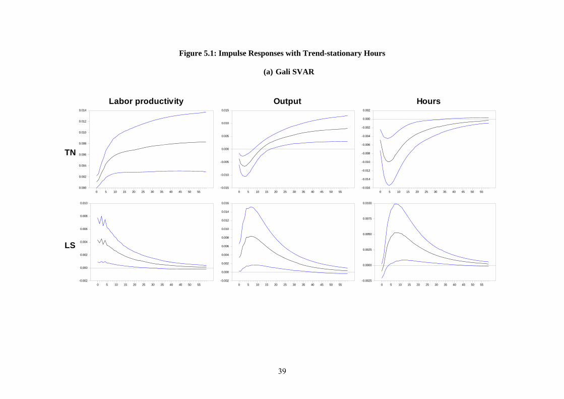
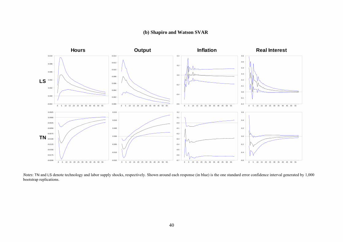
difference-stationary hours. Figures 5.1 and 5.2 display the impulse responses and historical

decompositions estimated from the Gali and SW models when hours worked is assumed to be

a trend-stationary process. For both models, the impulse responses remain largely unchanged

with two obvious exceptions; the transitory effects of the labor supply shock and the

responses of hours converging to zero in the long run, reflecting the assumption of the trend

stationary hours. Again, a positive technology shock leads to a decline in hours, analogous to

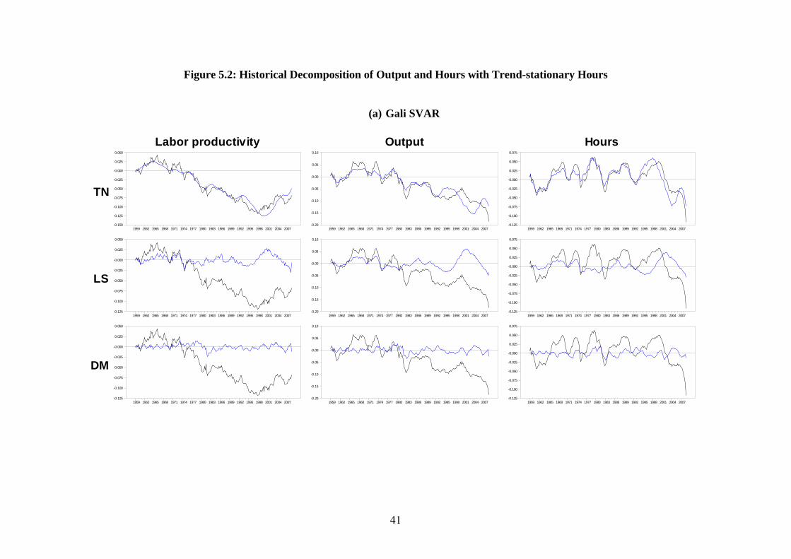
the finding under the assumption of difference-stationary hours. However, the historical

18

decomposition produces quite a different picture; across the models, the technology shock is

now the main source of movements in output, and the contribution of the labor supply shock

shrinks considerably, particularly since the mid-1970s. Similar changes are also observed for

explaining the variability of hours. Now, the technology shock emerges as the main

determinant while the labor supply shock contributes far less than before.

To further illustrate, we re-compute the conditional correlations of the structural

shocks with cyclical output under the assumption that hours worked is a trend-stationary

process. The results are reported in Tables 2.1 and 2.2. Several changes are worth discussion.

Examining the Gali model first, the technology shock is the most highly correlated with

cyclical output as documented by the correlation coefficient of 0.87. The correlation between

demand shocks and cyclical output is only about 0.2, which is quite low compared with the

correlation coefficient of 0.68 when hours was assumed to be difference-stationary. Even

when all non-technology shocks are combined, the correlation coefficient is just 0.33, far less

than the correlation between the technology shock and cyclical output.

The SW model produces the same implications. The correlation of cyclical output

with the technology shock rises considerably to 0.84, while the corresponding figure for

demand shocks is diminished to 0.37, in comparison to the result when hours was assumed to

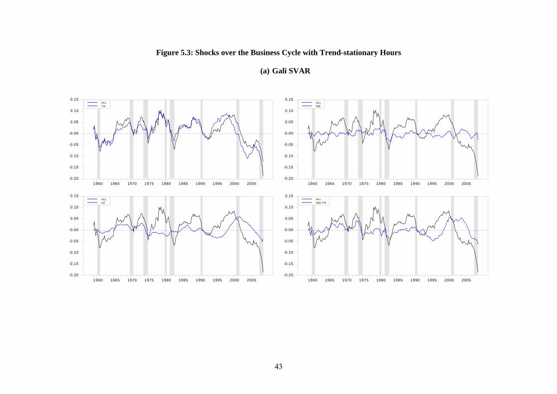
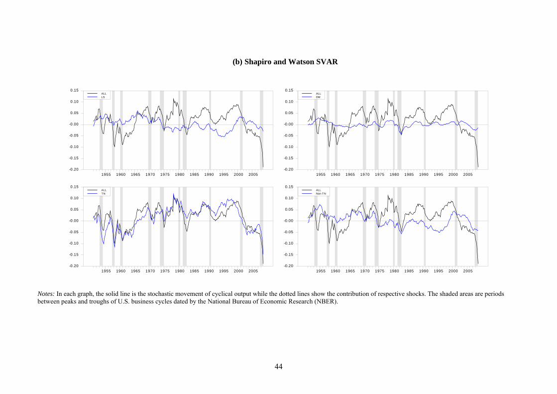
be difference-stationary. The historical decomposition of cyclical output reported in Figure

5.3 consolidates the results. The technology shock accounts for most of the movements in

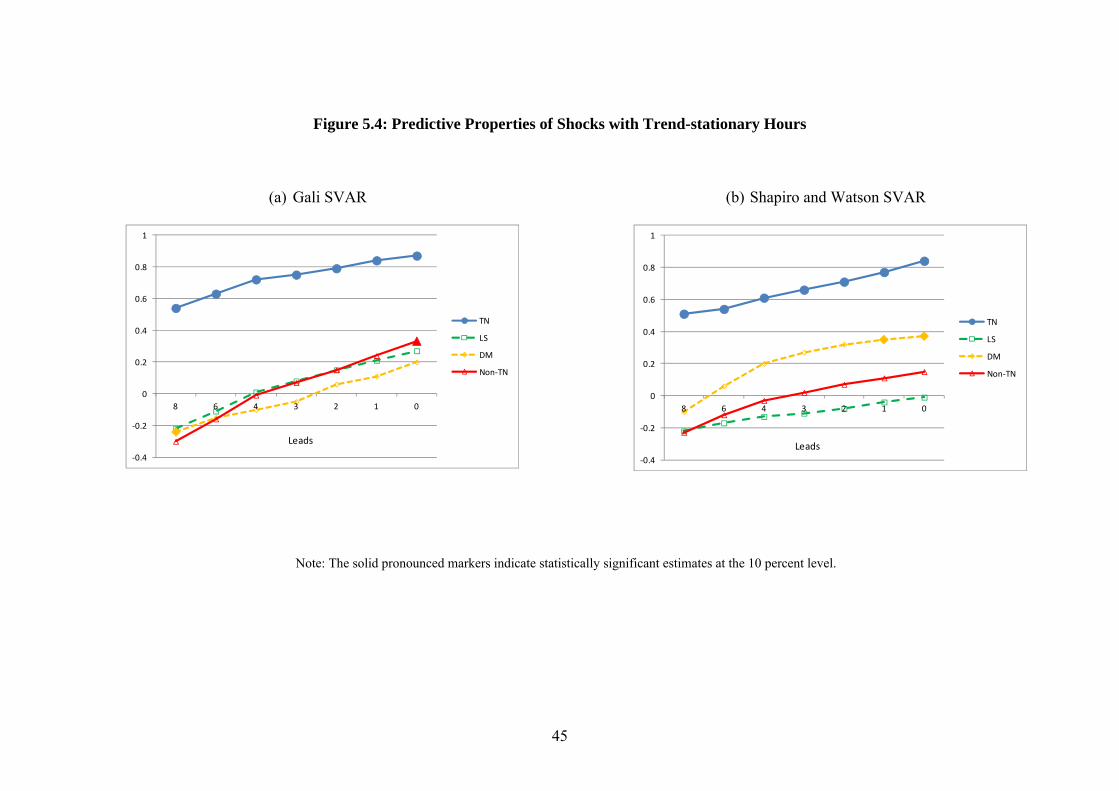
cyclical output, while both labor supply and demand shocks contribute little. Figure 5.4

shows that the predictive power of technology shocks is also strengthened under the

assumption of stationary hours. For both the Gali and SW models, the technology shock leads

cyclical output far better than labor supply and demand shocks across all leads, showing

particularly strong effects at short leads. Even over longer leads, such as eight quarters, the

coefficient remains higher than 0.5. For the SW model, demand shocks exhibit some

19

predictability at short leads but only marginally, while the labor supply shock fails to lead

cyclical output.

In summary, our results are sensitive to whether hours worked is assumed to be a

difference-stationary or trend-stationary process. The RBC hypothesis is more preferred

under the trend-stationarity assumption. In addition, the evidence is more pronounced when

we decompose the variables into permanent and transitory components and focus only on the

latter components, which reflect movements at business cycle frequencies. When hours

worked is assumed to be difference-stationary, technology and demand shocks are almost

equally important in accounting for cyclical output. Under the assumption of trend-stationary

hours, the technology shock becomes the major determinant of cyclical output, outperforming

all other shocks, including demand shocks. This finding provides rather strong support for

the RBC hypothesis. The results are robust for both Gali and SW models, despite the fact

that these models have different structures and identifying assumptions.7 Therefore, whether

hours worked is a difference-stationary or trend-stationary process may be a useful yardstick

for discriminating between RBC and New Keynesian models. Policy implications would

differ depending on which model is a better description of the real economy. While more

comprehensive research is warranted, it could be difficult to draw an empirical distinction

concerning the time-series properties of hours, given the well-known low power problem of

many unit root tests coupled with the typical sample size of macroeconomic data. Because

this issue is beyond the scope of the current paper, we leave it for future research and move

on to another related issue.

5.2. Technology shocks and hours worked

7 For example, the Gali model assumes that technology shocks can affect all of the variables in the long run, but labor supply shocks are not allowed to have a long-run effect on labor productivity. The converse is assumed in the SW model: labor supply shocks can have a long-run impact on all of the variables while technology shocks cannot have permanent effects on labor supply.

20

Gali (1999) argued that technology shocks lead to a decline in hours worked, whether hours

is difference-stationary or trend-stationary, using this as evidence against the RBC hypothesis.

In the impulse response analysis, we find results similar to those of Gali, as displayed in

Figures 1.1, 1.2, and 5.1. The figures also indicate that the decline in hours is present only in

the short time horizon, after which the responses of hours to a positive technology shock are

statistically insignificant (Figure 1.1) or converge to zero (Figures 1.2 and 5.1) by the

identifying assumptions. As stated earlier, the impulse response analysis reflects the

composite effects on both long-term movements and short-term dynamics. To isolate the

short-term from the long-term movements, the decomposition outlined in Section 3 was

applied to hours worked. In this way, we sought to determine whether Gali’s argument would

still hold once confined to movements at business cycle frequencies.

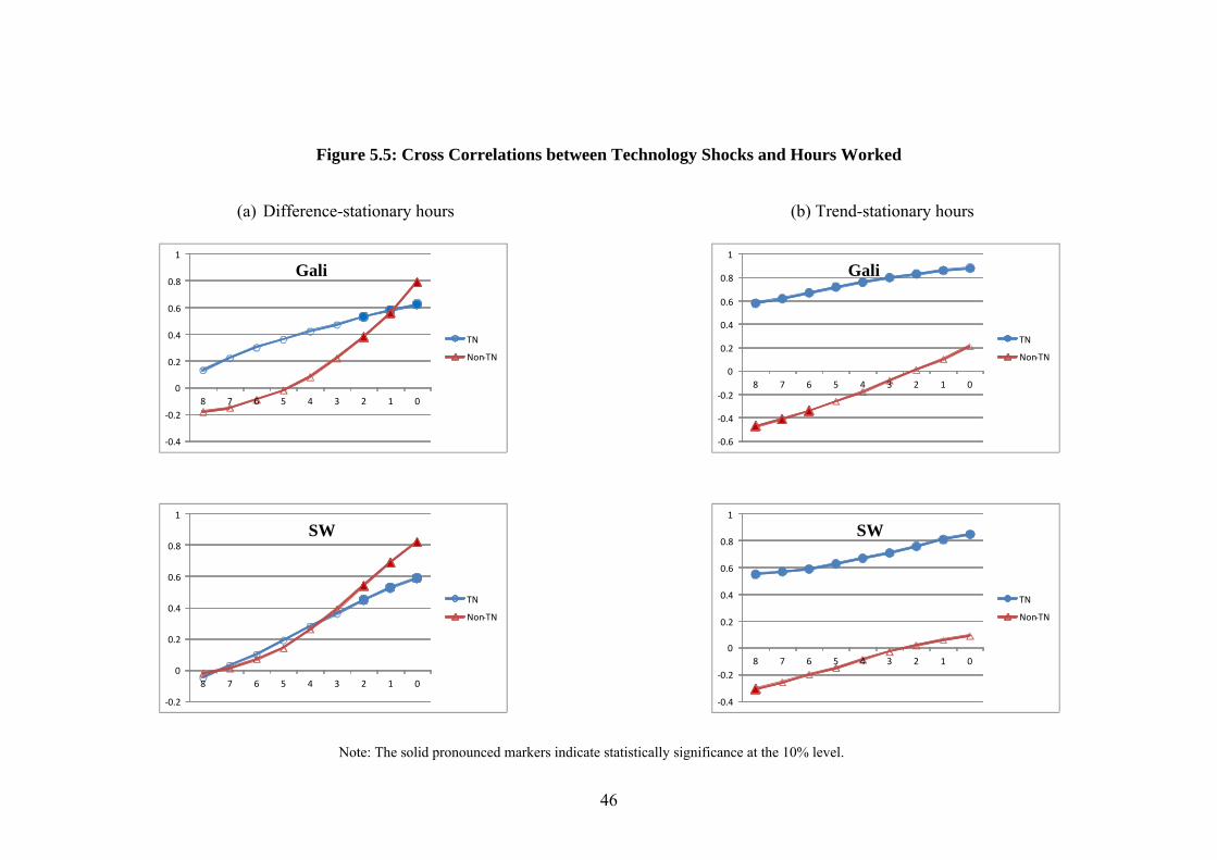
Figure 5.5 displays the conditional correlations between technology shocks and

cyclical hours over the leads of one to eight quarters. The technology shock appears to be

positively correlated with cyclical hours contemporaneously across the Gali and SW models.

This is robust whether hours worked is assumed to be a difference-stationary or trend-

stationary process. The correlations range between 0.59 and 0.88 and are particularly strong

under the trend-stationarity assumption. It is also notable that the Gali and SW models

produce coefficients of a very similar magnitude, validating the robustness of the results.

Furthermore, the technology shock is found to lead cyclical hours considerably, displaying

positive and statistically significant correlations at most of the leads. Thus, our evidence does

not support Gali’s finding that a positive technology shock leads to a decline in hours, when

examined over business cycle frequencies. Rather, our finding that a technology shock has a

strongly positive association with cyclical variation in hours is quite well explained by the

RBC models.8

8 In RBC models, a positive shock to technology leads to a rise in hours worked through an increase in the marginal product of labor and the consequent adjustments in the marginal rate of substitution.

21

6. Conclusion

This paper examined the empirical sources of business cycle fluctuations in the postwar U.S.

economy using three popular variants of SVAR models; those studied by Gali (1999),

Shapiro and Watson (1988), and King, Plosser, Stock and Watson (1991). In adopting these

models, a minimum set of theoretical restrictions were imposed a priori to avoid favoring a

particular theory, especially between New Keynesian and RBC paradigms. The current study

went significantly further than the original SVAR contributions by making extensive use of

the statistical properties of the data and results. In particular, the variables were decomposed

into permanent and transitory components; using the latter, we investigated the relationships

between underlying structural shocks and movements of the variables at business cycle

frequencies. This strategy appeared to pay economically interesting dividends. Technology

and demand shocks were both shown to be the most important sources of variation in cyclical

output. This finding is different from that suggested by the conventional impulse response

and historical decomposition analysis.

This paper also examined two important issues still being debated in the literature:

whether the assumption of stationarity of hours worked matters; and whether a positive

technology shock leads to a decline in hours, as claimed by Gali (1999). As to the first issue,

our results showed considerable changes under the assumption of trend-stationary hours. Of

particular interest, we found that a technology shock was the most important determinant of

cyclical output, while all other shocks, including demand shocks, showed only marginal

contributions. This study provided an equally interesting result with respect to the second

issue. While we, like other authors, found a decline in hours in response to a positive

technology shock, a very different picture emerged when focused on the movements over the

business cycle. The technology shock was positively correlated with the contemporaneous

and future values of cyclical hours, invalidating Gali’s claim. The effects were more

22

pronounced when hours was assumed to be trend-stationary. Our evidence is robust across

the models under consideration.

Considering all these results together, we conclude that technology shocks should not

be discarded as an important driver of business cycle fluctuations, nor should the RBC be

thrown out simply because of its emphasis on technology shocks. Although we may “forever

remain ignorant of the fundamental causes of economic fluctuations” as remarked by

Cochrane (1994b), technology shocks are never likely to be dropped as an important source

of macroeconomic fluctuations. The technology-driven real business cycle hypothesis should

be still alive.

23

References Beveridge, Stephen. and Nelson, Charles R. (1981) “A new approach to decomposition of

economic time series into permanent and transitory components with particular attention to measurement of the business cycle,” Journal of Monetary Economics 7(2), 151-174.

Chari, V.V., Kehoe, Patrick J. and McGrattan, Ellen R. (2008) “Are structural VARs with

long-run restrictions useful in developing business cycle theory?,” Journal of Monetary Economics 55(8), 1337-1352.

Chari, V.V., Kehoe, Patrick J. and McGrattan, Ellen R. (2009) “New Keynesian models: Not

yet useful for policy analysis,” American Economic Journal: Macroeconomics 1(1), 242-266.

Christiano, Lawrence J., Eichenbaum, Martin and Vigfusson, Robert. (2003) “What happens

after a technology shock?,” International Finance Discussion Papers 768, Board of Governors of the Federal Reserve System.

Christiano, Lawrence J., Eichenbaum, Martin and Vigfusson, Robert (2004) “The response of

hours to a technology shock: Evidence based on direct measures of technology,” Journal of the European Economic Association 2(2-3), 381-395.

Cochrane, John. (1994a) “Permanent and transitory components of GNP and stock prices,”

Quarterly Journal of Economics 109, 241-266. Cochrane, John. (1994b) “Shocks,” Carnegie-Rochester Conference Series on Public Policy

41, 295-364. Cogley, Timothy and Nason, James M. (1995) “Output dynamics in real-business-cycle

models,” American Economic Review 85(3), 492-511. Fama, Eugene F. (1992) “Transitory variation in investment and output,” Journal of

Monetary Economics 30(3), 467-480. Fisher, J. D. (2006), “The dynamic effects of neutral and investment‐specific technology

shocks”, Journal of Political Economy 114(3), 413-451. Fisher Lance A., Huh, Hyeon-Seung and Summers, Peter M. (2000), “Structural

Identification of Permanent Shocks in VEC Models: A Generalization,” Journal of Macroeconomics 22(1), 53-68.

Francis, Neville and Ramey, Valerie A. (2005) “Is the technology-driven real business cycle

hypothesis dead?: Shocks and aggregate fluctuations revisited,” Journal of Monetary Economics 52(8), 1379-1399.

Gali, Jordi. (1999) “Technology, employment, and the business cycle: do technology shocks

explain aggregate fluctuations?,” American Economic Review 89(1), 249-271. Gali, Jordi. (2004) “On the role of technology shock as a source of business cycles: Some

new evidence,” Journal of the European Economic Association 2(2-3), 372-380.

24

Gali, Jordi and Rabanal, Paul. (2004) “Technology shocks and aggregate fluctuations: How well does the RBC model fit postwar U.S. data?,” in M. Gertler and K. Rogoff (eds): NBER Macroeconomics Annual 2004, MIT Press, 225-288.

Gonzalo, Jesus and Ng, Serena. (2001) “A systematic framework for analyzing the dynamic

effects of permanent and transitory shocks,” Journal of Economic Dynamics and Control 25(10), 1527-1546.

King, Robert G., Plosser, Charles I., Stock, James H. and Watson, Mark W. (1991)

“Stochastic Trends and Economic Fluctuations,” American Economic Review 81(4), 819-840.

Kydland, Finn. and Prescott Edward C. (1982) “Time to build and aggregate fluctuations,”

Econometrica, 50(6), 1345- 1370. McGrattan, Ellen (2004) “Comment on Gali and Rabanal’s technology shocks and aggregate

fluctuations: How well does the RBC model fit postwar U.S. data?,” in M. Gertler and K. Rogoff (eds): NBER Macroeconomics Annual 2004, MIT Press, 289-308.

Pagan, Adrian R. and Pesaran, M. Hashem (2008) “Econometric analysis of structural

systems with permanent and transitory shocks,” Journal of Economic Dynamics and Control 32(10), 3376-3395.

Shapiro, Matthew and Watson, Mark. (1988) “Sources of business cycles fluctuations,” in S.

Fischer (ed.): NBER Macroeconomics Annual 1988, MIT Press, 111-148. Wang, Pengfei and Wen, Yi. (2011) “Understanding the effects of technology shocks”,

Review of Economic Dynamics 14(4), 705-724.

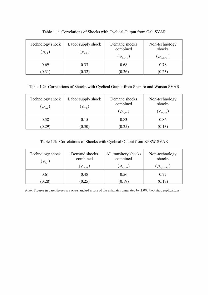
Table 1.1: Correlations of Shocks with Cyclical Output from Gali SVAR

Technology shock

( ,1v )

Labor supply shock

( ,2v )

Demand shocks combined

( ,345v )

Non-technology shocks

( ,2345v )

0.69

(0.31)

0.33

(0.32)

0.68

(0.26)

0.78

(0.23)

Table 1.2: Correlations of Shocks with Cyclical Output from Shapiro and Watson SVAR

Technology shock

( ,2v )

Labor supply shock

( ,1v )


( 34,v )


( 234,v )

0.58

(0.29)

0.15

(0.30)

0.83

(0.25)

0.86

(0.13)

Table 1.3: Correlations of Shocks with Cyclical Output from KPSW SVAR

Technology shock

( )


( 23,v )

All transitory shocks combined

( 456,v )


( 23456,v )

0.61

(0.28)

0.48

(0.25)

0.56

(0.19)

0.77

(0.17) Note: Figures in parentheses are one-standard errors of the estimates generated by 1,000 bootstrap replications.

,1v

26

Table 2.1: Correlations of Shocks with Cyclical Output from Gali SVAR (trend-stationary hours)

Technology shock

( ,1v )

Labor supply shock

( ,2v )


( ,345v )


( ,2345v )

0.87

(0.16)

0.27

(0.19)

0.20

(0.14)

0.33

(0.19)

Table 2.2: Correlations of Shocks with Cyclical Output from Shapiro and Watson SVAR (trend-stationary hours)

Technology shock

( ,2v )

Labor supply shock

( ,1v )


( 34,v )


( 234,v )

0.84

(0.17)

-0.01

(0.22)

0.37

(0.20)

0.15

(0.21) Note: Figures in parentheses are one-standard errors of the estimates generated by 1,000 bootstrap replications.

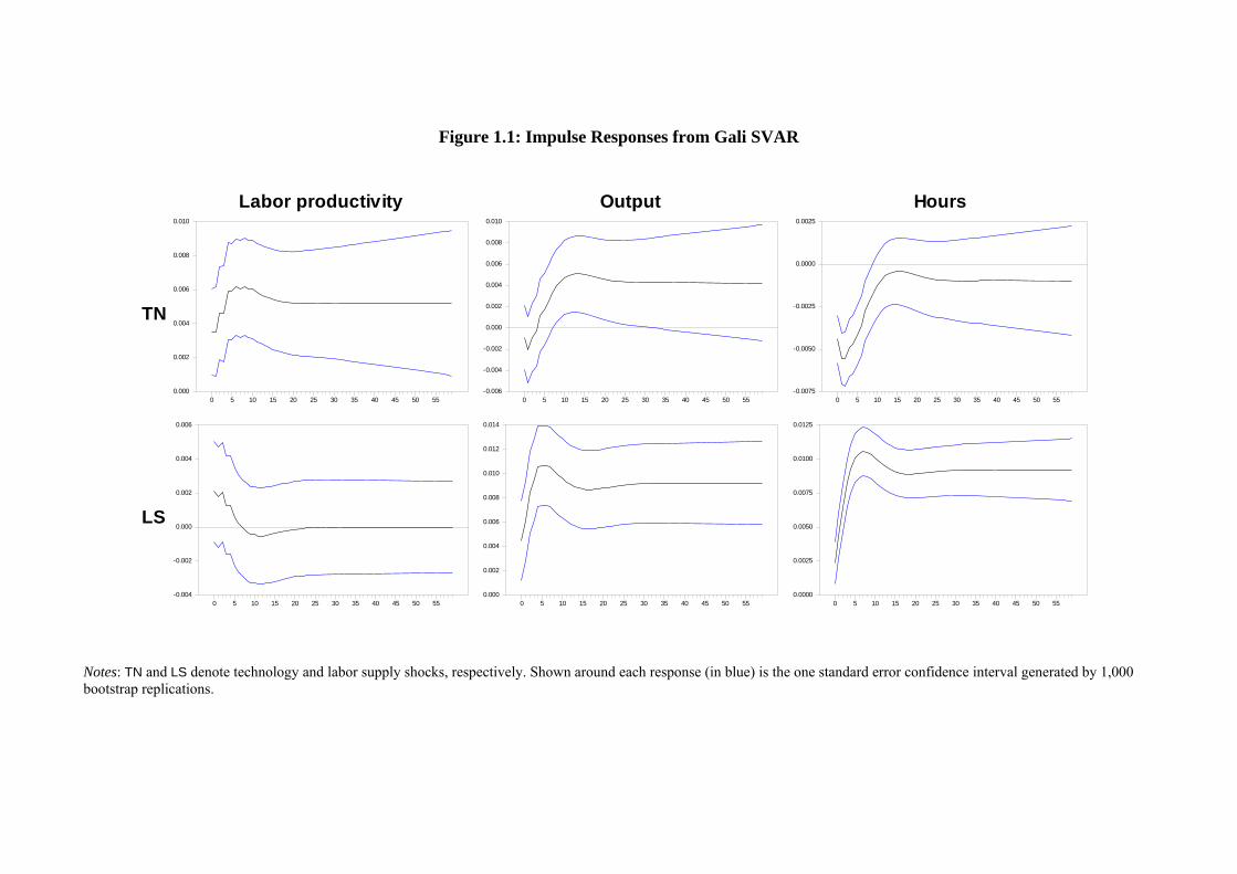
Figure 1.1: Impulse Responses from Gali SVAR

Notes: TN and LS denote technology and labor supply shocks, respectively. Shown around each response (in blue) is the one standard error confidence interval generated by 1,000 bootstrap replications.

TN

LS

Labor productivity Output Hours

0 5 10 15 20 25 30 35 40 45 50 550.000

0.002

0.004

0.006

0.008

0.010

0 5 10 15 20 25 30 35 40 45 50 55-0.004

-0.002

0.000

0.002

0.004

0.006

0 5 10 15 20 25 30 35 40 45 50 55-0.006

-0.004

-0.002

0.000

0.002

0.004

0.006

0.008

0.010

0 5 10 15 20 25 30 35 40 45 50 550.000

0.002

0.004

0.006

0.008

0.010

0.012

0.014

0 5 10 15 20 25 30 35 40 45 50 55-0.0075

-0.0050

-0.0025

0.0000

0.0025

0 5 10 15 20 25 30 35 40 45 50 550.0000

0.0025

0.0050

0.0075

0.0100

0.0125

28

Figure 1.2: Impulse Responses from Shapiro and Watson SVAR

Notes: LS and TN denote labor supply and technology shocks, respectively. Shown around each response (in blue) is the one standard error confidence interval generated by 1,000 bootstrap replications.

LS

TN

Hours Output Inflation Real Interest

0 5 10 15 20 25 30 35 40 45 50 550.0025

0.0050

0.0075

0.0100

0.0125

0.0150

0 5 10 15 20 25 30 35 40 45 50 55-0.0075

-0.0050

-0.0025

0.0000

0.0025

0 5 10 15 20 25 30 35 40 45 50 550.005

0.006

0.007

0.008

0.009

0.010

0.011

0.012

0.013

0 5 10 15 20 25 30 35 40 45 50 55-0.001

0.000

0.001

0.002

0.003

0.004

0.005

0.006

0.007

0 5 10 15 20 25 30 35 40 45 50 55-0.4

-0.2

0.0

0.2

0.4

0.6

0 5 10 15 20 25 30 35 40 45 50 55-1.0

-0.8

-0.6

-0.4

-0.2

-0.0

0.2

0 5 10 15 20 25 30 35 40 45 50 55-0.25

0.00

0.25

0.50

0.75

0 5 10 15 20 25 30 35 40 45 50 55-0.4

-0.2

0.0

0.2

0.4

0.6

0.8

29

Figure 1.3: Impulse Responses from KPSW SVAR

Notes: TN, IF, and RR denote shocks to technology, inflation, and real interest rate, respectively. Shown around each response (in blue) is the one standard error confidence interval generated by 1,000 bootstrap replications.

TN

IF

RR

Output Consumption Investment

0 5 10 15 20 25 30 35 40 45 50 550.0000

0.0025

0.0050

0.0075

0.0100

0.0125

0 5 10 15 20 25 30 35 40 45 50 55-0.002

-0.001

0.000

0.001

0.002

0.003

0.004

0.005

0.006

0 5 10 15 20 25 30 35 40 45 50 55-0.003

-0.002

-0.001

0.000

0.001

0.002

0.003

0.004

0.005

0.006

0 5 10 15 20 25 30 35 40 45 50 550.002

0.004

0.006

0.008

0.010

0.012

0 5 10 15 20 25 30 35 40 45 50 55-0.0020

-0.0015

-0.0010

-0.0005

0.0000

0.0005

0.0010

0.0015

0.0020

0 5 10 15 20 25 30 35 40 45 50 55-0.0005

0.0000

0.0005

0.0010

0.0015

0.0020

0.0025

0.0030

0.0035

0.0040

0 5 10 15 20 25 30 35 40 45 50 55-0.005

0.000

0.005

0.010

0.015

0.020

0.025

0.030

0.035

0 5 10 15 20 25 30 35 40 45 50 55-0.010

-0.005

0.000

0.005

0.010

0.015

0.020

0.025

0 5 10 15 20 25 30 35 40 45 50 55-0.020

-0.015

-0.010

-0.005

0.000

0.005

0.010

0.015

0.020

30

Figure 2.1: Historical Decompositions from Gali SVAR

Notes: In each graph, the solid line is the stochastic movement in a variable. The dotted lines show the contribution of the structural shocks where TN, LS, and DM denote shocks to technology, labor supply, and demand, respectively.

31

Figure 2.2: Historical Decompositions from Shapiro and Watson SVAR

Notes: In each graph, the solid line is the stochastic movement in a variable. The dotted lines show the contribution of the structural shocks where LS, TN, and DM denote shocks to labor supply, technology, and demand, respectively.

32

Figure 2.3: Historical Decompositions from KPSW SVAR

Notes: In each graph, the solid line is the stochastic movement in a variable. The dotted lines show the contribution of the structural shocks where TN, IF, RR, and TR denote technology shock, inflation shock, real interest rate shock, and transitory shocks, respectively.

33

Figure 3.1: Cyclical Output and Shocks from Gali SVAR

Notes: In each graph, the solid line is the stochastic movement of cyclical output, while the dotted lines show the contribution of respective shocks. The shaded areas are periods between peaks and troughs of U.S. business cycles dated by the National Bureau of Economic Research (NBER).

1960 1965 1970 1975 1980 1985 1990 1995 2000 2005-0.075

-0.050

-0.025

0.000

0.025

0.050ALLTN

1960 1965 1970 1975 1980 1985 1990 1995 2000 2005-0.075

-0.050

-0.025

0.000

0.025

0.050ALLLS

1960 1965 1970 1975 1980 1985 1990 1995 2000 2005-0.075

-0.050

-0.025

0.000

0.025

0.050ALLDM

1960 1965 1970 1975 1980 1985 1990 1995 2000 2005-0.075

-0.050

-0.025

0.000

0.025

0.050ALLNon-TN

34

Figure 3.2: Cyclical Output and Shocks from Shapiro and Watson SVAR


1955 1960 1965 1970 1975 1980 1985 1990 1995 2000 2005-0.06

-0.04

-0.02

0.00

0.02

0.04

0.06ALLLS

1955 1960 1965 1970 1975 1980 1985 1990 1995 2000 2005-0.06

-0.04

-0.02

0.00

0.02

0.04

0.06ALLTN

1955 1960 1965 1970 1975 1980 1985 1990 1995 2000 2005-0.06

-0.04

-0.02

0.00

0.02

0.04

0.06ALLDM

1955 1960 1965 1970 1975 1980 1985 1990 1995 2000 2005-0.06

-0.04

-0.02

0.00

0.02

0.04

0.06ALLNon-TN

35

Figure 3.3: Cyclical Output and Shocks from KPSW SVAR


1955 1960 1965 1970 1975 1980 1985 1990 1995 2000 2005-0.075

-0.050

-0.025

0.000

0.025

0.050

0.075ALLTN

1955 1960 1965 1970 1975 1980 1985 1990 1995 2000 2005-0.075

-0.050

-0.025

0.000

0.025

0.050

0.075ALLDM

1955 1960 1965 1970 1975 1980 1985 1990 1995 2000 2005-0.075

-0.050

-0.025

0.000

0.025

0.050

0.075ALLTR

1955 1960 1965 1970 1975 1980 1985 1990 1995 2000 2005-0.075

-0.050

-0.025

0.000

0.025

0.050

0.075ALLNon-TN

36

Figure 4.1: Predictive Properties of Shocks from Gali SVAR

Note: The solid pronounced markers indicate statistically significant point estimates at the 10 percent level.

‐0.2

0

0.2

0.4

0.6

0.8

1

8 6 4 3 2 1 0

TN

LS

DM

Non‐TN

Leads

Gali

37

Figure 4.2: Predictive Properties of Shocks from Shapiro and Watson SVAR


‐0.2

0

0.2

0.4

0.6

0.8

1

8 6 4 3 2 1 0

TN

LS

DM

Non‐TN

SW

Leads

38

Figure 4.3: Predictive Properties of Shocks from KPSW SVAR


‐0.2

0

0.2

0.4

0.6

0.8

1

8 6 4 3 2 1 0

TN

DM

TR

Non‐TN

KPSW

Leads

39

Figure 5.1: Impulse Responses with Trend-stationary Hours

(a) Gali SVAR

TN

LS


0 5 10 15 20 25 30 35 40 45 50 550.000

0.002

0.004

0.006

0.008

0.010

0.012

0.014

0 5 10 15 20 25 30 35 40 45 50 55-0.002

0.000

0.002

0.004

0.006

0.008

0.010

0 5 10 15 20 25 30 35 40 45 50 55-0.015

-0.010

-0.005

0.000

0.005

0.010

0.015

0 5 10 15 20 25 30 35 40 45 50 55-0.002

0.000

0.002

0.004

0.006

0.008

0.010

0.012

0.014

0.016

0 5 10 15 20 25 30 35 40 45 50 55-0.016

-0.014

-0.012

-0.010

-0.008

-0.006

-0.004

-0.002

0.000

0.002

0 5 10 15 20 25 30 35 40 45 50 55-0.0025

0.0000

0.0025

0.0050

0.0075

0.0100

40

(b) Shapiro and Watson SVAR

Notes: TN and LS denote technology and labor supply shocks, respectively. Shown around each response (in blue) is the one standard error confidence interval generated by 1,000 bootstrap replications.

LS

TN


0 5 10 15 20 25 30 35 40 45 50 55-0.002

0.000

0.002

0.004

0.006

0.008

0.010

0 5 10 15 20 25 30 35 40 45 50 55-0.0200

-0.0175

-0.0150

-0.0125

-0.0100

-0.0075

-0.0050

-0.0025

0.0000

0.0025

0 5 10 15 20 25 30 35 40 45 50 550.000

0.002

0.004

0.006

0.008

0.010

0.012

0.014

0 5 10 15 20 25 30 35 40 45 50 55-0.015

-0.010

-0.005

0.000

0.005

0.010

0.015

0 5 10 15 20 25 30 35 40 45 50 55-0.6

-0.4

-0.2

0.0

0.2

0.4

0 5 10 15 20 25 30 35 40 45 50 55-0.7

-0.6

-0.5

-0.4

-0.3

-0.2

-0.1

-0.0

0.1

0.2

0 5 10 15 20 25 30 35 40 45 50 55-0.2

-0.1

0.0

0.1

0.2

0.3

0.4

0.5

0.6

0 5 10 15 20 25 30 35 40 45 50 55-0.6

-0.4

-0.2

0.0

0.2

0.4

0.6

41

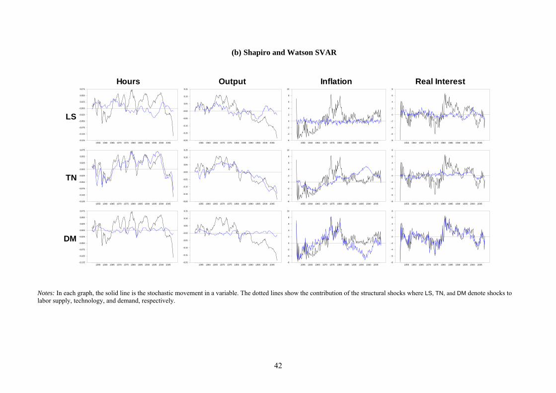
Figure 5.2: Historical Decomposition of Output and Hours with Trend-stationary Hours

(a) Gali SVAR

TN

LS

DM


1959 1962 1965 1968 1971 1974 1977 1980 1983 1986 1989 1992 1995 1998 2001 2004 2007-0.150

-0.125

-0.100

-0.075

-0.050

-0.025

-0.000

0.025

0.050

1959 1962 1965 1968 1971 1974 1977 1980 1983 1986 1989 1992 1995 1998 2001 2004 2007-0.20

-0.15

-0.10

-0.05

-0.00

0.05

0.10

1959 1962 1965 1968 1971 1974 1977 1980 1983 1986 1989 1992 1995 1998 2001 2004 2007-0.125

-0.100

-0.075

-0.050

-0.025

-0.000

0.025

0.050

0.075

1959 1962 1965 1968 1971 1974 1977 1980 1983 1986 1989 1992 1995 1998 2001 2004 2007-0.125

-0.100

-0.075

-0.050

-0.025

-0.000

0.025

0.050

1959 1962 1965 1968 1971 1974 1977 1980 1983 1986 1989 1992 1995 1998 2001 2004 2007-0.20

-0.15

-0.10

-0.05

-0.00

0.05

0.10

1959 1962 1965 1968 1971 1974 1977 1980 1983 1986 1989 1992 1995 1998 2001 2004 2007-0.125

-0.100

-0.075

-0.050

-0.025

-0.000

0.025

0.050

0.075

1959 1962 1965 1968 1971 1974 1977 1980 1983 1986 1989 1992 1995 1998 2001 2004 2007-0.125

-0.100

-0.075

-0.050

-0.025

-0.000

0.025

0.050

1959 1962 1965 1968 1971 1974 1977 1980 1983 1986 1989 1992 1995 1998 2001 2004 2007-0.20

-0.15

-0.10

-0.05

-0.00

0.05

0.10

1959 1962 1965 1968 1971 1974 1977 1980 1983 1986 1989 1992 1995 1998 2001 2004 2007-0.125

-0.100

-0.075

-0.050

-0.025

-0.000

0.025

0.050

0.075

42


Notes: In each graph, the solid line is the stochastic movement in a variable. The dotted lines show the contribution of the structural shocks where LS, TN, and DM denote shocks to labor supply, technology, and demand, respectively.

LS

TN

DM


1955 1960 1965 1970 1975 1980 1985 1990 1995 2000 2005-0.125

-0.100

-0.075

-0.050

-0.025

-0.000

0.025

0.050

0.075

1955 1960 1965 1970 1975 1980 1985 1990 1995 2000 2005-0.125

-0.100

-0.075

-0.050

-0.025

-0.000

0.025

0.050

0.075

1955 1960 1965 1970 1975 1980 1985 1990 1995 2000 2005-0.125

-0.100

-0.075

-0.050

-0.025

-0.000

0.025

0.050

0.075

1955 1960 1965 1970 1975 1980 1985 1990 1995 2000 2005-0.20

-0.15

-0.10

-0.05

-0.00

0.05

0.10

0.15

1955 1960 1965 1970 1975 1980 1985 1990 1995 2000 2005-0.20

-0.15

-0.10

-0.05

-0.00

0.05

0.10

0.15

1955 1960 1965 1970 1975 1980 1985 1990 1995 2000 2005-0.20

-0.15

-0.10

-0.05

-0.00

0.05

0.10

0.15

1955 1960 1965 1970 1975 1980 1985 1990 1995 2000 2005-6

-4

-2

0

2

4

6

8

10

1955 1960 1965 1970 1975 1980 1985 1990 1995 2000 2005-6

-4

-2

0

2

4

6

8

10

1955 1960 1965 1970 1975 1980 1985 1990 1995 2000 2005-6

-4

-2

0

2

4

6

8

10

1955 1960 1965 1970 1975 1980 1985 1990 1995 2000 2005-8

-6

-4

-2

0

2

4

6

8

1955 1960 1965 1970 1975 1980 1985 1990 1995 2000 2005-8

-6

-4

-2

0

2

4

6

8

1955 1960 1965 1970 1975 1980 1985 1990 1995 2000 2005-8

-6

-4

-2

0

2

4

6

8

43

Figure 5.3: Shocks over the Business Cycle with Trend-stationary Hours

(a) Gali SVAR

1960 1965 1970 1975 1980 1985 1990 1995 2000 2005-0.20

-0.15

-0.10

-0.05

-0.00

0.05

0.10

0.15ALLTN

1960 1965 1970 1975 1980 1985 1990 1995 2000 2005-0.20

-0.15

-0.10

-0.05

-0.00

0.05

0.10

0.15ALLLS

1960 1965 1970 1975 1980 1985 1990 1995 2000 2005-0.20

-0.15

-0.10

-0.05

-0.00

0.05

0.10

0.15ALLDM

1960 1965 1970 1975 1980 1985 1990 1995 2000 2005-0.20

-0.15

-0.10

-0.05

-0.00

0.05

0.10

0.15ALLNon-TN

44


Notes: In each graph, the solid line is the stochastic movement of cyclical output while the dotted lines show the contribution of respective shocks. The shaded areas are periods between peaks and troughs of U.S. business cycles dated by the National Bureau of Economic Research (NBER).

1955 1960 1965 1970 1975 1980 1985 1990 1995 2000 2005-0.20

-0.15

-0.10

-0.05

-0.00

0.05

0.10

0.15ALLLS

1955 1960 1965 1970 1975 1980 1985 1990 1995 2000 2005-0.20

-0.15

-0.10

-0.05

-0.00

0.05

0.10

0.15ALLTN

1955 1960 1965 1970 1975 1980 1985 1990 1995 2000 2005-0.20

-0.15

-0.10

-0.05

-0.00

0.05

0.10

0.15ALLDM

1955 1960 1965 1970 1975 1980 1985 1990 1995 2000 2005-0.20

-0.15

-0.10

-0.05

-0.00

0.05

0.10

0.15ALLNon-TN

45

Figure 5.4: Predictive Properties of Shocks with Trend-stationary Hours

(a) Gali SVAR


‐0.4

‐0.2

0

0.2

0.4

0.6

0.8

1

8 6 4 3 2 1 0

TN

LS

DM

Non‐TN

Leads

‐0.4

‐0.2

0

0.2

0.4

0.6

0.8

1

8 6 4 3 2 1 0

TN

LS

DM

Non‐TN

Leads

Note: The solid pronounced markers indicate statistically significant estimates at the 10 percent level.

46

Figure 5.5: Cross Correlations between Technology Shocks and Hours Worked

(a) Difference-stationary hours

(b) Trend-stationary hours

SW

‐0.4

‐0.2

0

0.2

0.4

0.6

0.8

1

8 7 6 5 4 3 2 1 0

TN

Non‐TN

Gali

‐0.6

‐0.4

‐0.2

0

0.2

0.4

0.6

0.8

1

8 7 6 5 4 3 2 1 0

TN

Non‐TN

SW

‐0.2

0

0.2

0.4

0.6

0.8

1

8 7 6 5 4 3 2 1 0

TN

Non‐TN

Gali

‐0.4

‐0.2

0

0.2

0.4

0.6

0.8

1

8 7 6 5 4 3 2 1 0

TN

Non‐TN

Note: The solid pronounced markers indicate statistically significance at the 10% level.

Documents

Shocks – Do SVAR Models Justify Discarding the Technology ... · Shocks – Do SVAR Models Justify Discarding the Technology Shock-Driven Real Business Cycle Hypothesis?† Hyeon-seung