Embed Size (px)
Citation preview

Short-Course: Introduction to regression analysis for
longitudinal data
(Part 1)
Instructor: Juan Carlos Salazar-Uribe*.
School of Statistics. Faculty of Sciences
National University of Colombia at Medellin
[email protected]*Educational Ambassador 2014-2015. Dr. Martha Aliaga’s Fund, American Statistical Asso-ciation. This material is largely based on Fitzmaurice, Laird, and Ware (2011). Applied Lon-gitudinal Analysis. 2nd Ed. Wiley: New Jersey. and JSM Professional Development ProgramContinuing Education Course on Applied Longitudinal Analysis. Other references were alsoused.
VII Summer school Medellın, Colombia, December 2015.
1

Abstract Short-Course
Longitudinal data are used both in research and in practice to try
to answer some questions about events that change or evolve
over time (eg cognitive skills of a senior citizen, the weight of a
person, the diameter of a tree, etc.). Linear mixed models have
become an indispensable tool for the analysis of longitudinal data.
VII Summer school Medellın, Colombia, December 2015.
2

Abstract Short-Course
In this short-course, it will be presented and discussed some li-
near mixed regression models adapted to situations where longi-
tudinal data arise. The first part of this short-course is dedicated
to presenting motivational examples where linear mixed regres-
sion models can be applied and further strategies for estimating
the parameters characterizing these models (Maximum likelihood
and restricted maximum likelihood ML REML) will be discussed.
VII Summer school Medellın, Colombia, December 2015.
3

Abstract Short-Course
Also, this first part includes examples of how these models can be
implemented using SAS. In the second part of this short-course
we will present some moderns approaches to model longitudinal
data using penalized splines as proposed by Fitzmaurice el at
(2011), finally, we study conditional and marginal linear mixed re-
gression models. Advantages and disadvantages of the presen-
ted methods are discussed.
VII Summer school Medellın, Colombia, December 2015.
4

Contents
Introduction and motivational examples, the classic lineal model,
longitudinal Data, Basic concepts, Fixed and random effects, Ma-
ximum likelihood estimation and Restricted maximum likelihood
estimation, regression model based on penalized splines, Condi-
tional models versus Marginal models. Examples.
VII Summer school Medellın, Colombia, December 2015.
5

Spruce tree growth data
(Kryscio, 2002) This experiment was conducted to compare the
growth of spruce trees under two environments: Control and Ozo-
ne enriched environment. There are 12 trees per group. For each
tree, 4 measures about growth were recorded at days 152, 174,
201 y 227, respectively. In other words, each tree contributes with
4 measures. The data set:
VII Summer school Medellın, Colombia, December 2015.
6

Spruce tree growth data
Obs Grupo Id y152 y174 y201 y2271 Control 1 2.79 3.10 3.30 3.382 Control 2 3.30 3.90 4.34 4.963 Control 3 3.98 4.36 4.79 4.994 Control 4 4.36 4.77 5.10 5.305 Control 5 4.34 4.95 5.42 5.976 Control 6 4.59 5.08 5.36 5.767 Control 7 4.41 4.56 4.95 5.238 Control 8 4.24 4.64 4.95 5.389 Control 9 4.82 5.17 5.76 6.1210 Control 10 3.84 4.17 4.67 4.6711 Control 11 4.07 4.31 4.90 5.1012 Control 12 4.28 4.80 5.27 5.55
VII Summer school Medellın, Colombia, December 2015.
7

Spruce tree growth data
Obs Grupo Id y152 y174 y201 y22713 Ozono 13 4.53 5.05 5.18 5.4114 Ozono 14 4.97 5.32 5.83 6.2915 Ozono 15 4.37 4.81 5.03 5.1916 Ozono 16 4.58 4.99 5.37 5.6817 Ozono 17 4.00 4.50 4.92 5.4418 Ozono 18 4.73 5.05 5.33 5.9219 Ozono 19 5.15 5.63 6.11 6.3920 Ozono 20 4.10 4.46 4.84 5.2921 Ozono 21 4.56 5.12 5.40 5.6922 Ozono 22 5.16 5.49 5.74 6.0523 Ozono 23 5.46 5.79 6.12 6.4124 Ozono 24 4.52 4.91 5.04 5.71
VII Summer school Medellın, Colombia, December 2015.
8
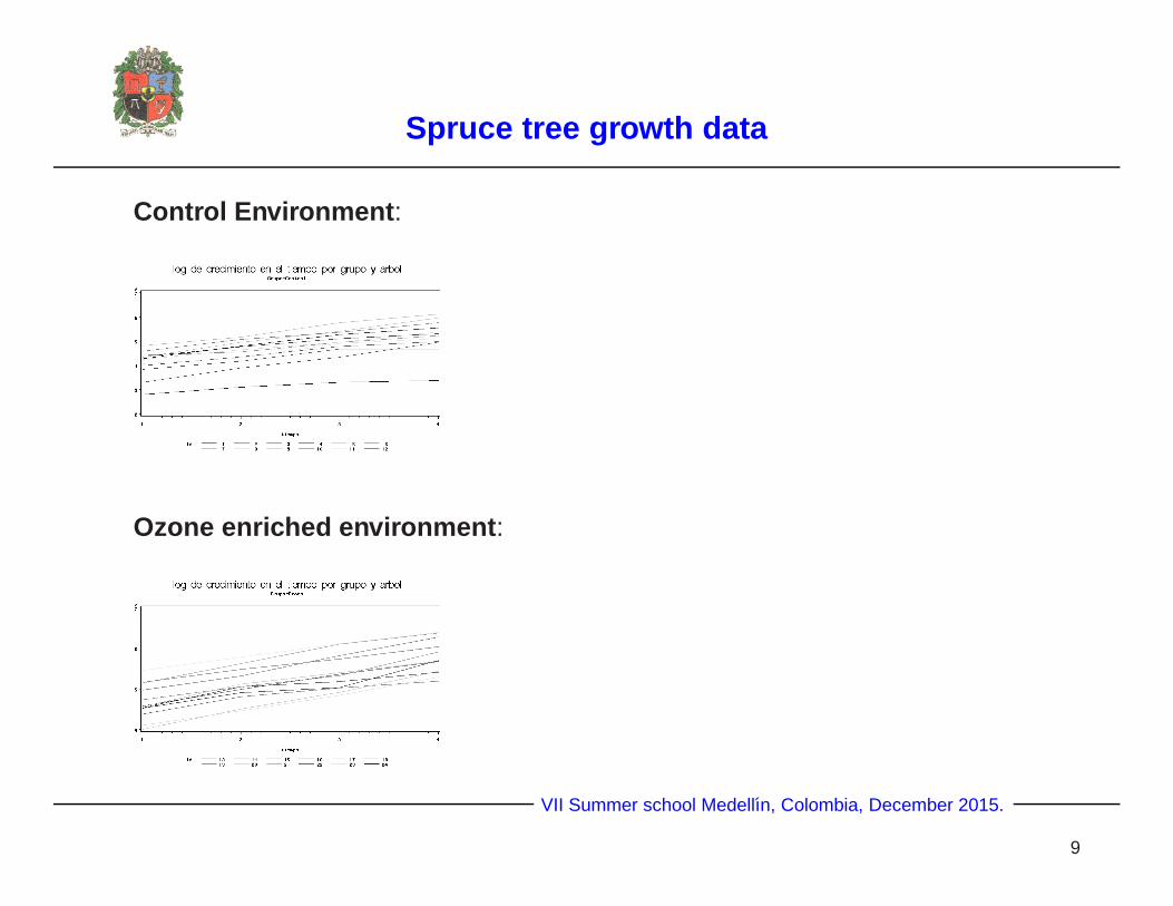
Spruce tree growth data
Control Environment :
Ozone enriched environment :
VII Summer school Medellın, Colombia, December 2015.
9

Spruce tree growth data
These plots show a linear trend over time and each tree seems to
have its own random intercept (the slopes seem to be the same).
The previous data set, will be used to illustrate different analysis
techniques typical in LMM.
VII Summer school Medellın, Colombia, December 2015.
10

Inference in the LMM
Example (Prostate Cancer). The Baltimore Longitudinal Study on Aging*.
This is a retrospective study. Prostate disease is one of the most common
and most costly medical problems in USA. Important to look for markers which
can detect the disease at an early age. Prostate-Specific Antigen (PSA)** is
an enzime produced by both normal and cancerous prostate cells. PSA level
is related to the volume of prostate tissue.
*References: Verbeke and Molenberghs (2000); Carter et al. (1992), Cancer Research; Mo-rrell et al. (1995), Journal of the American Statistical Association; Pearson at al. (1994),Statistics in Medicine
**High values of PSA mean high risk of prostate cancer
VII Summer school Medellın, Colombia, December 2015.
11

Inference in the LMM
Problem : Patients with Benign Prostatic Hyperplasia (BPH) also
have an increased PSA level. This produces an overlap in the
PSA distribution. In fact, this overlaping in the PSA distribution
for cancer and BPH cases seriously complicates the detection
of prostate cancer. The research question (hypothesis based on
clinical practice): Can longitudinal PSA profiles be used to de-
tect prostate cancer in an early stage? .
VII Summer school Medellın, Colombia, December 2015.
12

Inference in the LMM
In order to answer this important question, a retrospective case-control study
based on frozen serum samples was conducted. The study included 16 con-
trol patients, 20 BPH cases, 14 local cancer cases, 4 metastatic cancer cases
(more serious than local). Complication: No perfect match for age at diagno-
sis and years of follow-up possible*.
*Source : Stat Med. 1994 Mar 15-Apr 15;13(5-7):587-601. Mixed-effects regression models for studying thenatural history of prostate disease. Pearson JD, Morrell CH, Landis PK, Carter HB, Brant LJ. Abstract . Althoughprostate cancer and benign prostatic hyperplasia are major health problems in U.S. men, little is known aboutthe early stages of the natural history of prostate disease. A molecular biomarker called prostate specificantigen (PSA), together with a unique longitudinal bank of frozen serum, now allows a historic prospective studyof changes in PSA levels for decades prior to the diagnosis of prostate disease. Linear mixed-effects regressionmodels were used to test whether rates of change in PSA were different in men with and without prostatedisease. In addition, since the prostate cancer cases developed their tumours at different (and unknown) timesduring their periods of follow-up, a piece-wise non-linear mixed-effects regression model was used to estimatethe time when rapid increases in PSA were first observable beyond the background level of PSA change.These methods have a wide range of applications in biomedical research utilizing repeated measures datasuch as pharmacokinetic studies, crossover trials, growth and development studies, aging studies, and diseasedetection.
VII Summer school Medellın, Colombia, December 2015.
13

Inference in the LMM
Individual profiles:
VII Summer school Medellın, Colombia, December 2015.
14

Inference in the LMM
From previous plot we observe:
Much variability between subjects
Little variability within subjects
Highly unbalanced data
Not same number of subjects
Not linear trends
VII Summer school Medellın, Colombia, December 2015.
15

Treatment of Lead-Exposed Children Trial
(Fitzmaurice and Laird 2014)
Exposure of lead during infancy is associated with substantial deficits in test of cognitiveabilityChelation* treatment of children with high lead levels usually requires injections andhospitalizationsA new agent, Succimer, can be given orallyRandomized placebo-controlled trial examining changes in blood lead level during cour-se of treatment100 children randomized to placebo or SuccimerMeasures of blood lead level at baseline, 1, 4, and 6 weeks
*To remove (a heavy metal, such as lead or mercury) from the bloodstream by means ofa chelate, such as EDTA (Ethylenediaminetetracetic acid; a crystalline acid that acts as astrong chelating agent and that forms a sodium salt used as an antidote for metal poisoningand as an anticoagulant.)
VII Summer school Medellın, Colombia, December 2015.
16

Treatment of Lead-Exposed Children Trial
Treatment of Lead-Exposed Children Trial Data. Mean blood lead levels (and
SD) at baseline, week 1, 4, and 6.
Group Baseline Week 1 Week 4 Week 6Succimer 26.5 13.5 15.5 20.8
(5.0) (7.7) (7.8) (9.2)
Placebo 26.3 24.7 24.1 23.2(5.0) (5.5) (5.7) (6.2)
VII Summer school Medellın, Colombia, December 2015.
17

Treatment of Lead-Exposed Children Trial
Plot of mean blood lead levels at Baseline (Time=0), week 1, 4, and 6 in the
Succimer and Placebo groups
VII Summer school Medellın, Colombia, December 2015.
18

Example
Example. Progesterone metabolite concentration during me ns-
trual cycle *. Longitudinal data on PdG (pregnanediol-3-glucoronide)
measured daily in urine from day -8 to day 15 in the menstrual cy-
cle (day 0 denotes ovulation day).
*Brumback, B. and Rice, J. (1998). Smoothing spline models for the analysis of nested andcrossed samples of curves. Journal of the American Statistical Association, 93, 961−993
VII Summer school Medellın, Colombia, December 2015.
19

Example
A sample of 22 conceptive cycles from 22 women and 29 non-conceptive cy-
cles from another 29 women. Following standard practice in endocrinological
research, progesterone profiles are aligned by the day of ovulation, determi-
ned by serum luteinizing hormone, and then truncated at each end to yield
curves of equal length.
Measures are missing for certain cycles on some days. The goal is to describe
and compare the mean hormone profiles in the conceptive and non-conceptive
groups*, especially before and after implantation which occurs approx 7−8
days after ovulation.
*Using anti-pregnancy pills
VII Summer school Medellın, Colombia, December 2015.
20

Example
The following figures display time plots for the conceptive and non-conceptive groups. Figure12. (a) suggests that the trajectory of log progesterone concentration differs for the two groupsfollowing implantation (around day 7).
VII Summer school Medellın, Colombia, December 2015.
21

Alkaline battery duration
Six different brands of alkaline batteries were selected to study their dura-
tion under normal conditions: RAYOVAC c©, DURACELL c©, VARTA c©, ENER-
GIZER MAX c©, EVEREADY ALKALINE c©, PANASONIC POWER ALKALINE c©.
For each brand, 2 batteries were selected and they were plugged to a para-
llel especially designed to take the charge out from each battery. Every hour,
during 11 hours, the voltage were measured. The data is as follows:
RAYOVAC DURACELLVOLTAJE VOLTAGE
TIME Battery 1 Battery 2 Battery 1 Battery 20 1217 1288 1419 14501 1181 1248 1359 13932 1077 1170 1284 12963 1040 1138 1222 12354 1043 1099 1173 11785 1004 1047 1103 11066 949 968 877 8147 873 870 156 1388 780 740 107 1129 641 618 89 8410 62 62 71 7811 50 58 61 75
VII Summer school Medellın, Colombia, December 2015.
22

Alkaline battery duration
VARTA ENERGIZERVOLTAGE VOLTAGE
TIME Battery 1 Battery 2 Battery 1 Battery 20 1430 1308 1286 12681 1207 1150 1102 10602 1112 1052 1036 9953 1056 993 1000 9624 1025 953 972 9405 992 917 934 9056 952 818 874 8537 870 805 759 7638 246 172 166 109.29 96 77 75.4 70.410 69 65 62.6 6611 64 60 60.1 65.1
VII Summer school Medellın, Colombia, December 2015.
23

Alkaline battery duration
EVEREADY PANASONICVOLTAGE VOLTAGE
TIME Battery 1 Battery 2 Battery 1 Battery 20 1276 1212 1217 12791 1086 1001 1005 10442 1034 955 943 9803 992 910 897 9584 959 879 871 9305 886 844 804 8796 825 788 718 8237 693 679 602 7368 118.8 142.4 718 6129 75.5 75.1 602 95.510 64.7 64.3 117.6 7311 61.2 61.5 81.7 70.3
VII Summer school Medellın, Colombia, December 2015.
24

Alkaline battery duration
A profile plot of the data:
Figura 1. Profile plot of the data for the battery duration experiment. Around 5
hours it is observed a decay of the profiles associated to the different brands.
VII Summer school Medellın, Colombia, December 2015.
25

Longitudinal Data: Basic concepts
A defining feature of longitudinal studies is that measurements on the
same individuals are taken repeatedly through time
Longitudinal studies allow direct study of change over time
Primary goal is to characterize the changes in response over time and the
factors that influence change
With repeated measures, we can capture within-individual (or within-subject)
variability.
VII Summer school Medellın, Colombia, December 2015.
26

Longitudinal Data: Basic concepts
However, there are several complications when dealing with lon-
gitudinal data:
Repeated measures on individuals are correlated
Variability is often heterogeneous over time
VII Summer school Medellın, Colombia, December 2015.
27

Introduction
When the response variable is continuous, classical linear regres-
sion models can be extended to handle correlated outcomes that
are typical in longitudinal data. This correlation among repeated
measures could be modelled explicitly (e.g. via covariance pat-
tern models) or implicitly (via the introduction of random effect).
The latter approach yields a versatile class of regression models
for longitudinal data known as linear mixed effects models (Fitz-
maurice and Laird, 2014).
VII Summer school Medellın, Colombia, December 2015.
28

Introduction
LMM is a powerful statistical tool in applied research since it is not
only widely available in standard software but also it has a solid
and strong theoretical background. The term mixed model refers
to the nature of the parts of the model that explains the mean of
a statistical model.
VII Summer school Medellın, Colombia, December 2015.
29

Introduction
Usually in longitudinal data the outcome is observed repeatedly on different
times for each subject under study. Subjects are not necessarily observed
neither at the same time nor the same number of times (unbalanced data).
Covariates could also be different for each subject. These kind of data have
several features:
Each subject have a particular trend (or path) and they are not necessarily
straight lines.
If we obtain the average of all the observations we obtain an estimate of
the mean population profile
For this kind of longitudinal data it is formulated the so called subject specific
models or mean population models and depending of the goals of the study
one could be interested in one or another.
VII Summer school Medellın, Colombia, December 2015.
30

Introduction
Why to use LMM to model Longitudinal Data?
Because it is a flexible tool to model correlated data
Because estimation is based on likelihood function
Yields valid test in complex designs with unbalanced data
Allows REML estimation of variance components (Restricted Maximum Like-
lihood REML, to be discussed in detail later)
Allows inference of random effects
Available in R and SAS c©
VII Summer school Medellın, Colombia, December 2015.
31

Longitudinal and Panel data
Define yit to be the response for the ith subject during the tth time period.
A longitudinal data set consists of observations of the ith subject over t =
1,2, . . . ,T time periods, for each of i = 1,2, . . . ,n subjects. Thus, we observe:
First subject −{
y11,y12, . . . ,y1T1
}
Second subject −{
y21,y22, . . . ,y2T2
}
...
nth subject −{
yn1,yn2, . . . ,ynTn
}
VII Summer school Medellın, Colombia, December 2015.
32

General Linear Model (GLM)
(Littell at al. 2000) Statistical Models for data are descriptions on how the data
could be produced and they basically consist of two parts: (1) a formula relating
the response to all explanatory variable (e.g. effects), and (2) a description of
the probability distribution assumed to characterize random variation affecting
the observed response.
VII Summer school Medellın, Colombia, December 2015.
33

GLM
The GLM in matrix form
Y = Xβ+ ε
where
ε ∼ MN(
E(ε) = O, Σε = σ2I)
The Ordinary Least Squares (OLS) estimator for β is
β =(X′X
)−1X′Y
If Σε = σ2V where V is known
β =(
X′V−1X)−1
X′V−1Y (Generalized least squares estimator)
VII Summer school Medellın, Colombia, December 2015.
34

Linear mixed model LMM
This GLM can be extended to obtain a LMM that can be written
in a more precise way:
Yi = Xiβ+Zibi+ εi
bi ∼ N(0,D)
εi ∼ N(0,Σi)
b1, . . . ,bm,ε1, . . . ,εm : mutually independent
VII Summer school Medellın, Colombia, December 2015.
35

Linear mixed model LMM
Terminology :
β: Fixed effects.
bi and εi: Random effects.
Variance components: Elements of the matrices D and Σi
VII Summer school Medellın, Colombia, December 2015.
36

Special formulations of LMM
Random intercept model . This is one of the most common formulations of
the LMM. Each subject have a profile which is approximately parallel to the
trend of a particular group (Recall the Sitka Spruce data example). This model
can be expressed as:
yi j = β0+β1Ti j +β2Gi +β3Gi ×Ti j +b0i + εi j
where
The subject is represented by i: i = 1,2, · · · ,N.
Observations for subject j : j = 1,2, · · · ,mi .
b0i ∼ N(
0,σ2b
). εi j ∼ N
(0,σ2
ε
). b0i indep. of εi j
VII Summer school Medellın, Colombia, December 2015.
37

Alternative way of formulating the LMM
Recall the classic linear model*:
Yn×1 = Xn×kβk×1+ en×1
E (e) = 0
Var(e) = σ2I
e ∼ N(
0, σ2I)
Then:
E (Y) = E (Xβ+ e) = XβVar(Y) = Var(e) = σ2I
Y ∼ Nn
(Xβ, σ2I
)
*Machiavelli, R. (2014) Introduccion a los modelos mixtos. Proceedings X Coloquio de Es-tadıstica. Medellın, Colombia.
VII Summer school Medellın, Colombia, December 2015.
38

Randomized block design
The random intercepts model can be obtained from a design of experiments
theory point of view as follows. When we are studying the influence of a factor
over a quantitative factor (response) it is common to find other variables or
factors influencing that response and they must be controlled. These variables
are known as blocks. These blocks have the following properties:
(i) To study their effect is not a direct goal but they appear in a natural fashion
in the study.
(ii) They do not interact with the factor of interest.
VII Summer school Medellın, Colombia, December 2015.
39

Randomized block design
Classic model: Yi j = µ+ τi +ei j
Versus
Mixed model (Randomized block design): Yi j = µ+ τi +b j +ei j
(Similar to random intercept model)
b j and ei j are normally distributed.
VII Summer school Medellın, Colombia, December 2015.
40

Special formulations of LMM
Random intercepts and slopes model
This is perhaps the other most used LMM. Each subject differs to the others
in terms of both the intercept and the trend (slope) of the group. The model is
expressed as:
yi j = β0+β1Ti j +β2Gi +β3Gi ×Ti j +b0i +b1iTi j + εi j
where
εi j ∼ N(
0,σ2ε)
and[
b0ib1i
]∼ N
([00
],
[σ2
b0σb0,b1
σb0,b1σ2
b1
])
VII Summer school Medellın, Colombia, December 2015.
41

Special formulations of LMM
In matrix form:
yi1yi2...
yini
=
1 Ti1 Gi Gi ×Ti11 Ti2 Gi Gi ×Ti2... ... ... ...1 Tini
Gi Gi ×Tini
β0β1β2β3
+
1 Ti11 Ti2... ...1 Tini
[
b0i
b1i
]+
εi1εi2...
εini
yi = Xiβ+Zibi + εi
with Var(yi) = ZiDZ′i +σ2
εIni . Notice that when no random effects are speci-
fied Var(yi) = σ2εIni .
VII Summer school Medellın, Colombia, December 2015.
42

More on LMM
When an effect is either fixed or random?
If the studied levels are the only ones we are interested in, the effect could be
considered as fixed (e.g. the effect of a specific diet)
If the studied levels correspond to a random sample from a set of possible
levels, the effect could be considered as random (e.g. the effect of weight
groups)
VII Summer school Medellın, Colombia, December 2015.
43

More on Longitudinal Data
Let us suppose for a moment that we have not specified random effects. If
we have N independent units, then the matrix Σ will have a block diagonal
structure:
Σ =
Σ1 ,0 , . . . ,00 ,Σ2 , . . . ,0... ... ... ...0 ,0 . . . ,ΣN
Each of these blocks corresponds to a particular experimental unit and it will
have a structure reflecting both the variances and covariances within that unit.
VII Summer school Medellın, Colombia, December 2015.
44
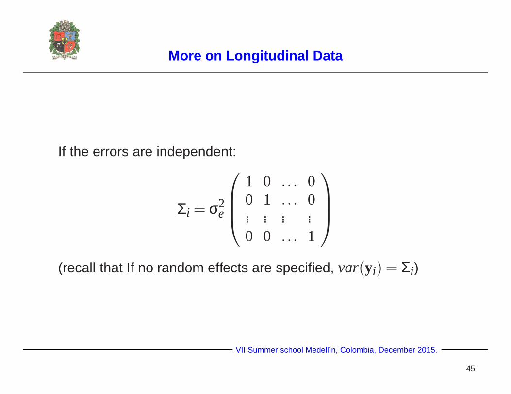
More on Longitudinal Data
If the errors are independent:
Σi = σ2e
1 0 . . . 00 1 . . . 0... ... ... ...0 0 . . . 1
(recall that If no random effects are specified, var(yi) = Σi)
VII Summer school Medellın, Colombia, December 2015.
45

More on Longitudinal Data
On the other hand, if we specified random effects and the so ca-
lled compound symmetry structure:
Var(yi) = Vi =(
σ2b+σ2
e
)
1 ρ . . . ρρ 1 . . . ρ... ... ... ...ρ ρ . . . 1
If ρ > 0, this is equivalent to think about Σi as independent and
add a random intercept at the subject’s level. The variances are
homogeneous. There is a correlation between two separate mea-
surements, but it is assumed that the correlation is constant re-
gardless of how far apart the measurements are.VII Summer school Medellın, Colombia, December 2015.
46

More on Longitudinal Data
Autoregressive of order 1 (AR(1)*, valid if observations are equi-spaced):
Var(yi) = Vi = σ2e
1 ρ ρ2 . . . ρT−1
ρ 1 ρ . . . ρT−2
ρ2 ρ 1 . . . ρT−3
... ... ... ... ...ρT−1 ρT−2 ρT−3 . . . 1
If observations are not equi-spaced one can use:
Corr(
ej ,ej ′)= ρ
∣∣∣t j−t j ′
∣∣∣, j 6= j ′
*The AR(1) structure has homogeneous variances and correlations that decline exponentially with distance. Itmeans that the variability in a measurement, say white blood cell count, is constant regardless of when youmeasure it. It also means that two measurements that are right next to each other in time are going to be prettycorrelated (depending on the value of ρ ), but that as measurements get farther and farther apart they are lesscorrelated.
VII Summer school Medellın, Colombia, December 2015.
47

More on Longitudinal Data
Selecting a covariance structure . To select models for the mean is a neces-
sary task. One approach consists in adjusting different covariance structures
and random effects (matrices D and Σ) and then, by means of a suitable crite-
ria (such as LRT, BIC, AIC) we choose the one suggested by the the criterium.
VII Summer school Medellın, Colombia, December 2015.
48

More on Longitudinal Data
Strategy of analysis . Once the structure for the covariance has been selected
we check again the fixed part of the model. For example, when we are fitting a
regression model, we first select variables, then we check assumptions. Then
we interpret the estimated coefficients, test the null hypotheses and draw con-
clusions. In the ANOVA we interpret interactions, compare means and test
contrasts to draw conclusions.
VII Summer school Medellın, Colombia, December 2015.
49

Inference in the LMM
Recall the formulations for the LMM:
Y = Xβ+Zb+ e[
be
]∼ N
([00
],
[D 00 Σ
])
E (Y) = Xβ, V (Y) = V = ZDZ′+Σ
VII Summer school Medellın, Colombia, December 2015.
50

Inference in the LMM
The conditional model :
Y|b ∼ N (Xβ+Zb, Σ)
b ∼ N (0,D)
E (Y|b) = Xβ+Zb, V (Y|b) = Σ
VII Summer school Medellın, Colombia, December 2015.
51

Inference in the LMM
The system of Henderson’s equations (Henderson, 1975) is useful for obtai-
ning estimates for and predictions for both β and b, respectively*:
X′Σ−1Xβ+X′Σ−1Zb = X′Σ−1Y(Z′Σ−1Z+D−1
)b+Z′Σ−1Xβ = Z′Σ−1Y
*Henderson’s Advice to Beginning Scientists: Study methods of your predecessors. Workhard. Do not fear to try new ideas. Discuss your ideas with others freely. Be quick to admiterrors. Progress comes by correcting mistakes. Always be optimistic. Nature is benign. Enjoyyour scientific work, it can be a great joy
VII Summer school Medellın, Colombia, December 2015.
52

Inference in the LMM
Solving this system, yields
β =(
X′V−1X)−1
X′V−1Y
The solution for b will be
b = DZ′V−1(
Y−Xβ)
which is the Best Linear Unbiased Predictor (BLUP) for b*
*BLUP’s are used to ’estimate’ random effects. BLUP’s are similar to BLUE’s (Best LinearUnbiased Estimator) of fixed effects. The difference is that we estimate fixed effects andpredict random effects, however, the equation for one or another are different.
VII Summer school Medellın, Colombia, December 2015.
53

Inference in the LMM
Maximum likelihood estimation
Notation : β: Vector of fixed effects
α: Vector of the components of variance in D y Σ
θ = (β, α): Vector of parameters in the marginal model (fixed effects and va-
riance components, respectively).
VII Summer school Medellın, Colombia, December 2015.
54

Inference in the LMM
By means of a process known as profiling we could find estimates for the fixed
effects. Profiled likelihood If v(β,α |Y) is twice the negative of the marginal
log-likelihood
−2log(β,α |Y)= log(|V(α)|)+(Y−Xβ)′V−1 (α)(Y−Xβ)+T log(2π) (4)
and it must be minimized with respect to β y α (the quantity T log(2π) does
not affect the maximization of the log-likelihood function process, since it is a
constant). This can be done by means of profiling with respect to β:
In this process we find a closed expression for β and it is substituted in
v(β,α |Y). i.e v(
β(α),α |Y)
The resultant expression will be a function of α and it is twice the negative
of the profiled likelihood.
VII Summer school Medellın, Colombia, December 2015.
55

Inference in the LMM
Marginal likelihood function :
LML (θ) =m
∏i=1
{(2π)−
ni2 |Vi(α)|−
12 e
−12
((Yi−Xiβ)′V−1
i (α)(Yi−Xiβ))}
If α is known, the MLE of β are:
β(α) =
(m
∑i=1
X′iWiXi
)−1 m
∑i=1
X′iWiXi
where Wi = V−1i . However, in general α is unknown and it is necessary to
replace it by an estimator α which is obtained either by maximum likelihood
(ML) or restricted maximum likelihood (REML)*. Using ML, one can obtained
αML maximizing LML
(α, β(α)
), with respect to α. The resultant estimator
β(αML) for β it is denoted as βML (process known as profiling).
*REML will be discussed ahead
VII Summer school Medellın, Colombia, December 2015.
56

Inference in the LMM
αML and βML can also be obtained from maximizing LML(θ = (α,β)) with
respect to θ, i.e., with respect to α and β simultaneously. Estimation of both
the fixed and variance components by ML was uncommon due to computatio-
nal difficulties related with the solution of the resultant systems of equations.
Harville (1977) review previous works, unified the theory and built iterative ML
algorithms for obtaining estimates of the parameters. In addition to the numeri-
cal problems, the estimators of the variance components obtained by ML, tend
to be biased.
VII Summer school Medellın, Colombia, December 2015.
57

Inference in the LMM
Restricted maximum likelihood estimation (REML) The question is: How
to estimate the variance components and not having to estimate the corres-
ponding parameters for the fixed effects? The answer leads to the so called
Restricted Maximum Likelihood Estimation (REML) proposed by Patterson y
Thompson (1971). By using this strategy the vector of fixed effects, β is drop-
ped from the log-likelihood function.
VII Summer school Medellın, Colombia, December 2015.
58

Inference in the LMM
In general, the only thing we need is a transformation of the data orthogonal
to X. In other words, we need residuals:
r = A′Y ∼ N(0,A′V(θ)A
)
The restricted likelihood function does not depend on β. Substituting into the
generalized least square estimator of β this REML estimator we obtain the
fixed effects estimator β(θREML) which is denoted as βREML.
In other words, we transform Y in such a way that the linear predictor Xβvanishes from the likelihood
r = A′Y ∼ N(0,A′V(θ)A
)
VII Summer school Medellın, Colombia, December 2015.
59

Inference in the LMM
Two examples of matrix A could be: Consider a sample of n observationsY1,Y2, . . . ,Yn from a N(µ,σ2)
1)
r = A′Y =
1 −1 · · · 0 0 00 1 −1 · · · 0 0... ... ... ... ... ...0 0 0 0 1 −1
Y1Y2...Yn
=
Y1−Y2Y2−Y3...Yn−1−Yn
2)
r=A′Y=
1− 1n −1
n · · · −1n −1
n −1n
−1n 1− 1
n −1n · · · −1
n −1n... ... ... ... ... ...
1n −1
n −1n −1
n −1n 1− 1
n
Y1Y2...Yn
=
Y1−YY2−Y...Yn−1−Y
In both cases, matrix A corresponds to the first n−1 rows of some matrix M.
VII Summer school Medellın, Colombia, December 2015.
60

Inference in the LMM
Usually M can be chosen as:
M = I−X(X′X
)−1X′
M could also be formulated as
M = V−1− V−1X(X′X
)−1X′V−1
Where V is some estimator of V =Cov(Y)).
Note : SAS and R use this last formulation for matrix M.
VII Summer school Medellın, Colombia, December 2015.
61

Inference in the LMM
These REML equations yields an estimator for α only. The estimators for the
fixed effects are estimated by using generalized mean squares, once one have
αR, as
βR=(
X′V−1(αR)X)−1
X′V−1(αR)Y
VII Summer school Medellın, Colombia, December 2015.
62

Inference in the LMM
SAS PROC MIXED constructs an objective function associated with ML or
REML and maximizes it over all unknown parameters. Using calculus, it is
possible to reduce this maximization problem to one over only the parameters
in D and Σ. The corresponding log-likelihood functions are as follows:
ML : ℓ(D,Σ) =−12
log|V|−12
r′V−1r−n2
log(2π)
REML: ℓR(D,Σ) =−12
log|V|−12
log|X′V−1X|−12
r′V−1r−n− p
2log(2π)}
where r = y−X(
X′V−1X)−1
X′V−1y, and p is the rank of X.
VII Summer school Medellın, Colombia, December 2015.
63

Inference in the LMM
Harville’s formulation for the likelihood
Harville (1974), showed that the log-likelihood function for the set of contrastscould be written as,
ℓ(α,A′Y
)= c−
12
log
∣∣∣∣∣m
∑i=1
X′iV
−1i Xi
∣∣∣∣∣−12
m
∑i=1
|Vi|−12
m
∑i=1
(Yi −Xiβ
)′V−1
i
(Yi −Xiβ
)
where c is a constant and β = β(α) as defined previously. To find a matrix A is
not a problem: any matrix of dimension (T− r)×T with T− r rows linearly
independent of M can be used , (Harville, 1977).
VII Summer school Medellın, Colombia, December 2015.
64
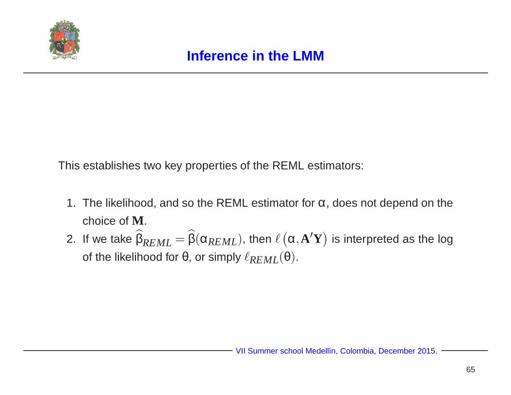
Inference in the LMM
This establishes two key properties of the REML estimators:
1. The likelihood, and so the REML estimator for α, does not depend on the
choice of M.
2. If we take βREML= β(αREML), then ℓ(α,A′Y
)is interpreted as the log
of the likelihood for θ, or simply ℓREML(θ).
VII Summer school Medellın, Colombia, December 2015.
65
Inference in the LMM
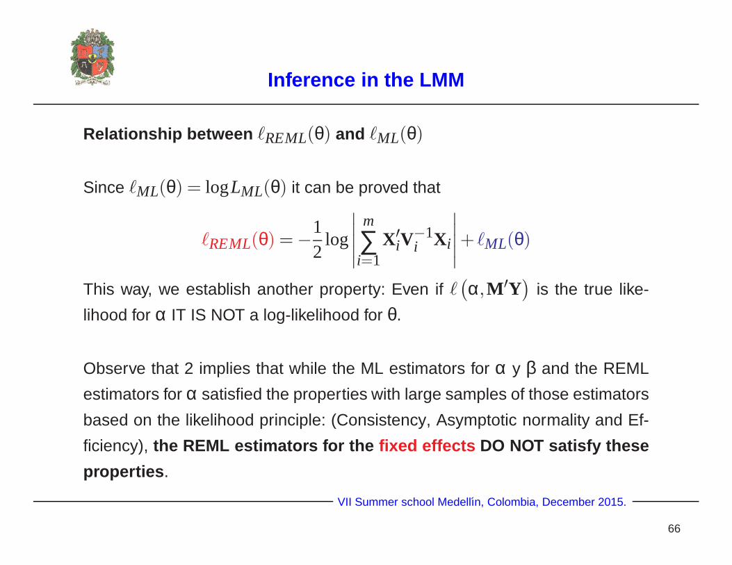
Relationship between ℓREML(θ) and ℓML(θ)
Since ℓML(θ) = logLML(θ) it can be proved that
ℓREML(θ) =−12
log
∣∣∣∣∣m
∑i=1
X′iV
−1i Xi
∣∣∣∣∣+ ℓML(θ)
This way, we establish another property: Even if ℓ(α,M′Y
)is the true like-
lihood for α IT IS NOT a log-likelihood for θ.
Observe that 2 implies that while the ML estimators for α y β and the REML
estimators for α satisfied the properties with large samples of those estimators
based on the likelihood principle: (Consistency, Asymptotic normality and Ef-
ficiency), the REML estimators for the fixed effects DO NOT satisfy these
properties .
VII Summer school Medellın, Colombia, December 2015.
66

Inference in the LMM
On the other hand, for mixed balanced ANOVA designs, it is known that the
REML estimators of the variance components are equal to the classic esti-
mator for the component variance obtained by the method of moments. This
generates a robustness property of the REML estimators agains violations of
the normality assumption.
Theoretical justification for the REML estimators
According to Patterson and Thompson (1971) and Harville and Jeske (1992),
if there are not information about β, we do not loose information about α when
the inference is based in A′Y instead of Y only.
From a bayesian point of view, to use just contrasts to make inference about
α, is equivalent to ignore any a priori information about β and use all the data
to make those inferences.VII Summer school Medellın, Colombia, December 2015.
67

Inference in the LMM
(Verbeke and Molenberghs 2009). Maximum likelihood estimation and restric-
ted maximum likelihood estimation both have the same merits of being based
on the likelihood principle which leads to useful properties such as consistency,
asymptotic normality, and efficiency (valid also for the REML estimates of the
Variance components). ML estimation also provides estimators of the fixed ef-
fects, whereas REML estimation, in itself, does not (the reason for this is that
REML yield estimators for the variance components). On the other hand, for
balanced mixed ANOVA models, the REML estimates for the variance compo-
nents are identical to classical ANOVA-type estimates obtained from solving
the equations which set mean squares equal to their expectations.
VII Summer school Medellın, Colombia, December 2015.
68

Inference in the LMM
This implies optimal minimum variance properties, and it shows that REML
estimates in that context do not rely on any normality assumption since only
moment assumptions are involved (Harville 1977, Searle 1992). Also with re-
gard to the mean squared error for estimating α, there is not clear preference
for either one of the two estimation procedures, since it depends on the speci-
fics of the underlying model and possibly on the true value of α.
VII Summer school Medellın, Colombia, December 2015.
69

Inference in the LMM
For ordinary ANOVA or regression models, the ML estimator of the residual va-
riance σ2e has uniformly smaller mean squared error than the REML estimator
when p= rank(X)≤ 4, but the opposite is true when p> 4 and n− p is suffi-
ciently large (indeed n− p> 2 suffices if p> 12). In general, one may expect
results from ML and REML estimation to differ more as the numb er p of
fixed effects in the model increases .
VII Summer school Medellın, Colombia, December 2015.
70

Inference in the LMM
Once the likelihood function is built (either by ML or REML) we
can use a numerical method to obtain the maximum θ. This can
be done by means of the Newton-Raphson algorithm (Lindstrom
and Bates, (1988)), the Expectation-Maximization algorithm (Dem-
pster et al. 1977), or the Simplex of Nelder-Mead (Nelder and
Mead, 1965). Monte Carlo Markov Chain based methods can al-
so be used and they today they are becoming very popular.
VII Summer school Medellın, Colombia, December 2015.
71
Example: Sitka-Spruce
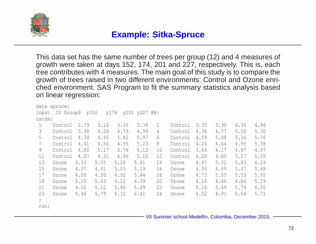
This data set has the same number of trees per group (12) and 4 measures ofgrowth were taken at days 152, 174, 201 and 227, respectively. This is, eachtree contributes with 4 measures. The main goal of this study is to compare thegrowth of trees raised in two different environments: Control and Ozone enri-ched environment. SAS Program to fit the summary statistics analysis basedon linear regression:
data spruce;input ID Group$ y152 y174 y201 y227 @@;cards;1 Control 2.79 3.10 3.30 3.38 2 Control 3.30 3.90 4.34 4.963 Control 3.98 4.36 4.79 4.99 4 Control 4.36 4.77 5.10 5.305 Control 4.34 4.95 5.42 5.97 6 Control 4.59 5.08 5.36 5.767 Control 4.41 4.56 4.95 5.23 8 Control 4.24 4.64 4.95 5.389 Control 4.82 5.17 5.76 6.12 10 Control 3.84 4.17 4.67 4.6711 Control 4.07 4.31 4.90 5.10 12 Control 4.28 4.80 5.27 5.5513 Ozone 4.53 5.05 5.18 5.41 14 Ozone 4.97 5.32 5.83 6.2915 Ozone 4.37 4.81 5.03 5.19 16 Ozone 4.58 4.99 5.37 5.6817 Ozone 4.00 4.50 4.92 5.44 18 Ozone 4.73 5.05 5.33 5.9219 Ozone 5.15 5.63 6.11 6.39 20 Ozone 4.10 4.46 4.84 5.2921 Ozone 4.56 5.12 5.40 5.69 22 Ozone 5.16 5.49 5.74 6.0523 Ozone 5.46 5.79 6.12 6.41 24 Ozone 4.52 4.91 5.04 5.71;run;
VII Summer school Medellın, Colombia, December 2015.
72

Example
data spruce1;set spruce;array xx(4) y152 y174 y201 y227;do i=1 to 4;log_growth=xx{i};if i=1 then time1=152;if i=2 then time1=174;if i=3 then time1=201;if i=4 then time1=227;output;
end;run;proc sort data=spruce1;by id;run;
VII Summer school Medellın, Colombia, December 2015.
73

Example
Consider the Sitka-Spruce trees data. First we are going to fit the followingmodel with REML as the estimation method:
proc mixed data=spruce1 method=REML;class group id;model log_growth=group time1 / solution;repeated / subject=id type=cs;lsmeans group / pdiff;title ’A variance component model with same marginal distribution’;title ’REML’;run;
VII Summer school Medellın, Colombia, December 2015.
74

Example
This program yields
USING REMLSolucion para efectos fijos
ErrorEfecto Group Estimador estandar DF Valor t Pr > |t|
Intercept 2.4783 0.1759 22 14.09 <.0001Group Control -0.5746 0.2139 22 -2.69 0.0135Group Ozone 0 . . . .time1 0.01466 0.000477 71 30.77 <.0001
Tests de tipo 3 de efectos fijosNum Den
Efecto DF DF F-Valor Pr > F
Group 1 22 7.22 0.0135time1 1 71 946.76 <.0001
VII Summer school Medellın, Colombia, December 2015.
75

Example
USING REMLMedias de minimos cuadrados
ErrorEfecto Group Estimador estandar DF Valor t Pr > |t|Group Control 4.6677 0.1512 22 30.86 <.0001Group Ozone 5.2423 0.1512 22 34.66 <.0001
Diferencias de medias de minimos cuadradosError
Efecto Group _Group Estimador estandar DF Valor t Pr > |t|Group Control Ozone -0.5746 0.2139 22 -2.69 0.0135
VII Summer school Medellın, Colombia, December 2015.
76

Example
Now we fit the following model with ML as the estimation method:
proc mixed data=spruce1 method=ML;class group id;model log_growth=group time1 / solution;repeated / subject=id type=cs;lsmeans group / pdiff;title ’A variance component model with same marginal distribution’;title ’ML’;run;
VII Summer school Medellın, Colombia, December 2015.
77

Example
This program yields
USING ML
Solucion para efectos fijos
ErrorEfecto Group Estimador estandar DF Valor t Pr > |t|Intercept 2.4783 0.1701 22 14.57 <.0001Group Control -0.5746 0.2048 22 -2.81 0.0103Group Ozone 0 . . . .time1 0.01466 0.000473 71 30.99 <.0001
Tests de tipo 3 de efectos fijos
Num DenEfecto DF DF F-Valor Pr > FGroup 1 22 7.87 0.0103time1 1 71 960.09 <.0001
VII Summer school Medellın, Colombia, December 2015.
78

Example
USING REMLMedias de minimos cuadrados
ErrorEfecto Group Estimador estandar DF Valor t Pr > |t|Group Control 4.6677 0.1512 22 30.86 <.0001Group Ozone 5.2423 0.1512 22 34.66 <.0001
Diferencias de medias de minimos cuadradosError
Efecto Group _Group Estimador estandar DF Valor t Pr > |t|Group Control Ozone -0.5746 0.2139 22 -2.69 0.0135
VII Summer school Medellın, Colombia, December 2015.
79

Example
Notice that there are differences in some p-values, standard errors
as well as between the values for some tests. For instance, the
estimated standard error for the parameter of the Control group
using REML is 0.2139 whereas the one obtained using ML is
0.2048 (values for the t-test are also different: -2.69 versus -2.81).
But we have to admit that there are not substantial differences in
the estimates obtained by using either REMl or ML (a possible
reason for this is that n>p).
VII Summer school Medellın, Colombia, December 2015.
80