Short Course

The Basics of Inversion

Bill MenkeColumbia University

1. The power of simple linear models

2. Probability and what it has to do with data analysis

3. Inferences using Least-Squares

4. Examples

Lectures

MatLab Scripts for all calculations in these lectures

www.ldeo.columbia.edu/users/menkecourses.html

Lecture 1

The power of simple, linear models

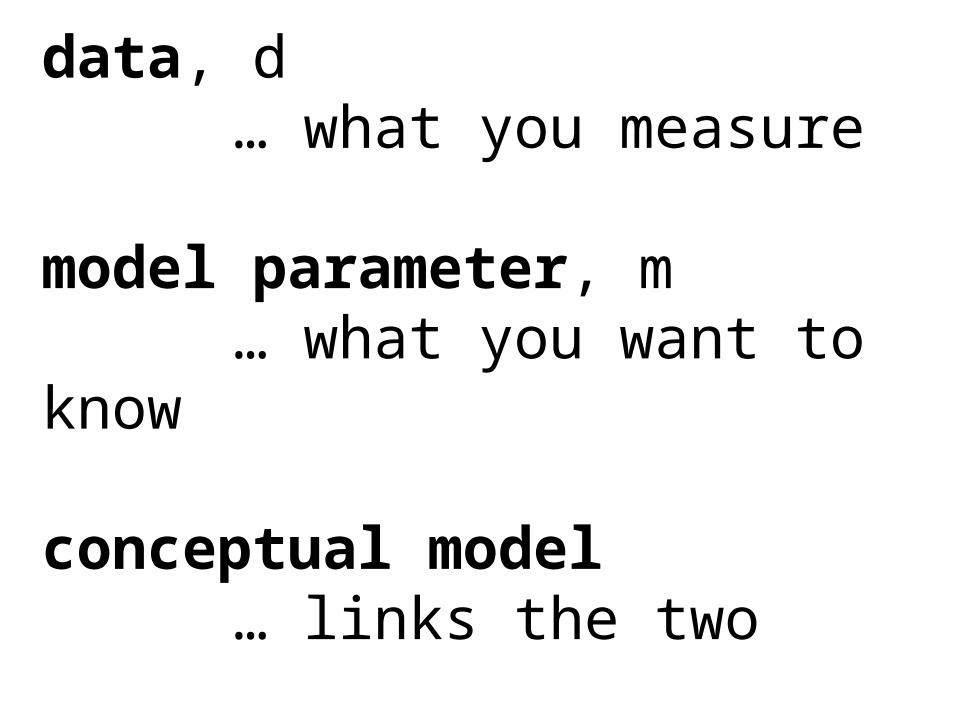
data, d… what you measure

model parameter, m… what you want to know

conceptual model… links the two

At the start of a project, spend a few moments identifying

datamodel parametersconceptual model

think about the strengths and weaknesses of each

Example – seismic tomography of the earth’s mantle

data: traveltimes of shear wavesbut the seismometer measured wiggles …

model parameter: shear velocity in mantlebut I really wanted to know temperatureshear velocity is just a proxy for temperature

conceptual modelray theory, an approximation to how vibrations

travel through the earth

example: river flow and rain

data: discharge on a succession of days,d1, d2, d3, …

model parameters: rain on a succession of daysm1, m2, m3, …

conceptual model:watershed with rain and transport

di = fcn( mi, mi-1, mi-2, …)

Causal: discharge depends only on present and past rain

example: CO2 and combustion of fossil fuels

data: CO2 on a succession of days,d1, d2, d3, …

model parameters: combustion rate on a succession of days

m1, m2, m3, …

conceptual model: global carbon cycle (transport, storage in biosphere and oceans, etc)

di = fcn( mi, mi-1, mi-2, …)

example: gravity anomaly and the earth’s density

data: strength of gravity on a 2D grid of points on the earth’s surface

d1, d2, d3, …

model parameters: density of the earth on a 3D grid of points in the earth’s interior

m1, m2, m3, …

conceptual model: Newton’s third law: mass causes gravitational attraction

di = fcn(mi+1, mi, mi-1, …)

not causal

example: straight line relationship

d

x

data: d1, d2, d3, …

model parameters: the slope and intercept of the linem1, m2

conceptual model: data are on a line:

di = m1 + m2 xi

or if you preferdi = a + b xi

In all these examplesthe data are linearly related to the

model parameters

(at least to first approximation)

Data: d= d1

d2

…

dN

model parameters: m=

m1

m2

…

mM

Linear model: d = Gm“data kernel” matrix

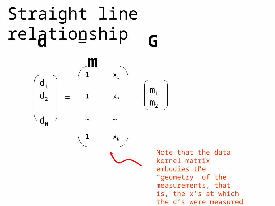
Straight line relationship

d1

d2

…

dN

=

d = G m

Note that the data kernel matrix embodies the “geometry” of the measurements, that is, the x’s at which the d’s were measured

1 x1

1 x2

… …

1 xN

m1

m2

Gravity anomaliesd: gravity anomaly in vertical directionm: density anomaly of a small cube of volume Dv

Newton’s Inverse-square Law:

di = cubes v mj cosij/ |xi - yj|2

gravitational constant

di

xi

yi

miij

Gravity anomalies

d1

d2

…

dN

=

d = G m

vertical component of gravity anomaly measured at position xi

m1

m2

…

mM

Z1111

Z12 … Z1M

Z21 Z22 … Z2M

… … … …

ZN1 ZN2 … ZNM

Newton’s law: zij = v cosij / |xi - yj|2

density anomalyof small cube of volume v located at position yi

once again, G embodies “geometry”

Thinking About Error

error = observed data – predicted data

e = dobs – dpre

= dobs – Gmest

always plot your data and look at the error!

Guess values for a, bypre = aguess + bguessx

aguess=2.0

bguess=2.4

Prediction error =

observed minus predicted

e = dobs - dpre

Total error: sum of squared predictions errors

E = Σ ei2

= eT e

Systematically examine combinations of (a, b) on a 101101 grid

Error Surface

Minimum total error E is here

Note E is not zero

bpre

apre

Error Surface

Note Emin is not zero Here are best-fitting a, b

best-fitting line

Note some range of values where the error is about the same as the minimun value, Emin

Error Surface

Emin is here

Error pretty close to Emin everywhere in here

All a’s in this range and b’s in this range have pretty much the same error

conclusion

the shape of the error surface

controls the accuracy by which (a,b) can be estimated

What controls the shape of theerror surface?

Let’s examine effect of increasing the error in the data

Error in data = 0.5

Error in data = 5.0

Emin = 0.20

Emin = 23.5

The minimum error increases, but the shape of the error surface is pretty much the same

0 5-5

0 5-5

What controls the shape of theerror surface?

Let’s examine effect of shifting the x-position of the data

0 105

Big change by simply shifting x-values of the data

Region of low error is now tilted

(High b, low a) has low error

(Low b, high a) has low error

But (high b, high a) and (low a, low b) have high error

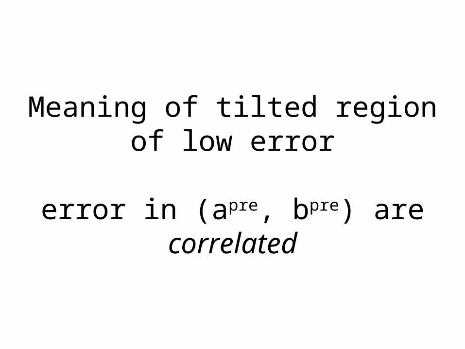
Meaning of tilted region of low error

error in (apre, bpre) arecorrelated

Best-fit

line

Best fit intercept

erroneous intercept

When the data straddle the origin, if you tweak the intercept up, you can’t compensate by changing the slope

Best-fit

line

Uncorrelated estimates of intercept and slope

Best-fit

line

Best fit intercept

Low slope line

erroneous intercept

When the data are all to the right of the origin, if you tweak the intercept up, you must lower the slope to compensate

Same slope s

Best-fit

line

Negatively correlation of intercept and slope

Best-fit

line

Best fit intercept

erroneous intercept

When the data are all to the left of the origin, if you tweak the intercept up, you must raise the slope to compensate

Same slope as b

est-fit

line

Positive correlation of intercept and slope

Best fit intercept

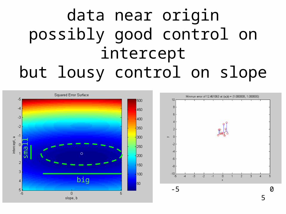
data near originpossibly good control on intercept

but lousy control on slope

-5 0 5

smal

l

big

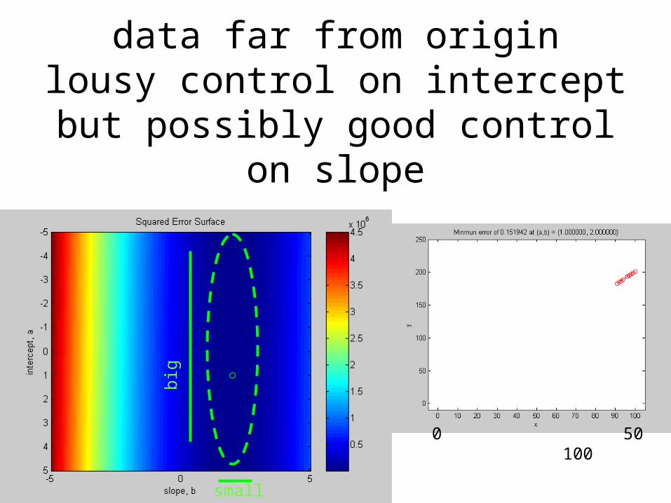
data far from originlousy control on intercept

but possibly good control on slope

small

big

0 50 100

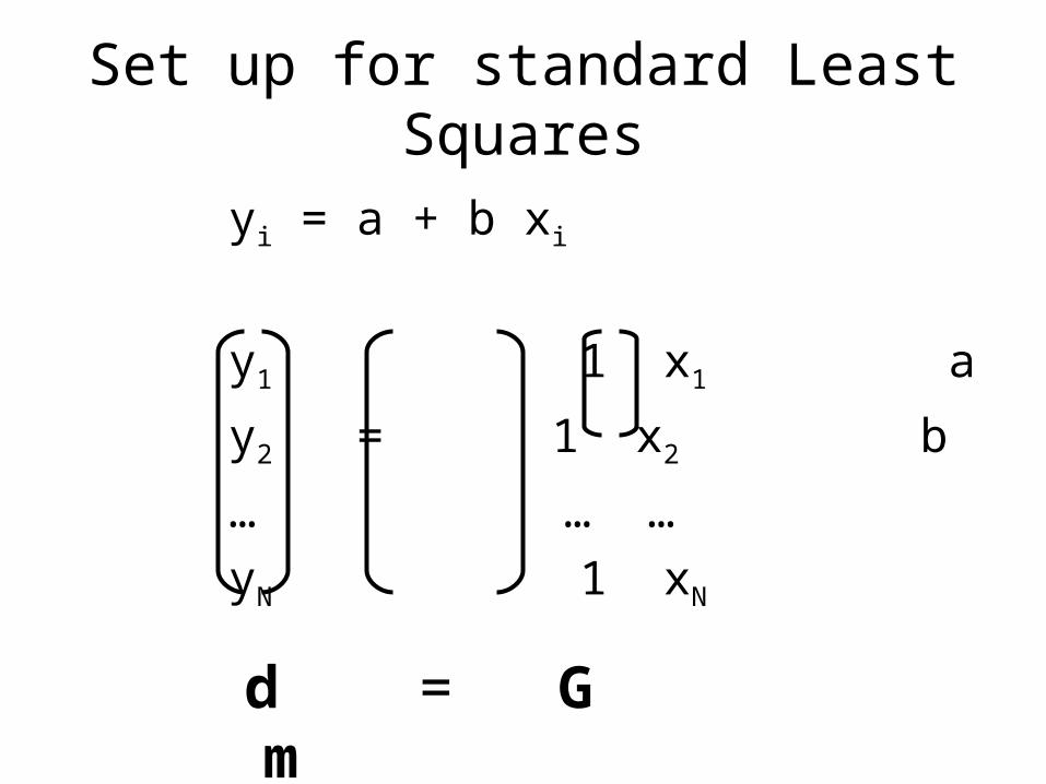
Set up for standard Least Squares

yi = a + b xi

y1 1 x1 a

y2 = 1 x2 b

… … …

yN 1 xN

d = G m

The formula for the least-squares solution for the general linear problem

is known:

mest = [GTG]-1 GT d

derived by a standard minimization procedure using calculus

Find the m that minimizes E(m) with E=eTe and e=d-Gm

Why least-squares? E=i ei2

Why not least-absolute length? E=i |ei|

Or something else?

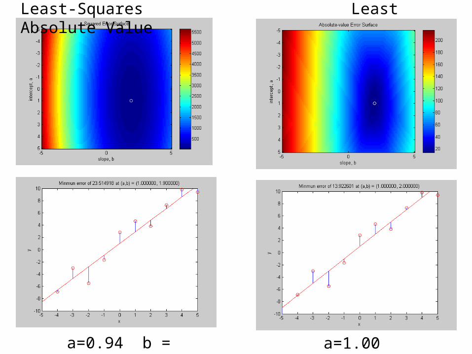
Least-Squares Least Absolute Value

a=1.00 b=2.02 a=0.94 b = 2.02