Short-Term Forecasting of Inflation in Bangladesh with Seasonal

Munich Personal RePEc Archive

Short-Term Forecasting of Inflation in

Bangladesh with Seasonal ARIMA

Processes

Akhter, Tahsina

10 January 2013

Online at https://mpra.ub.uni-muenchen.de/43729/

MPRA Paper No. 43729, posted 15 Jan 2013 20:04 UTC

Short-Term Forecasting of Inflation in Bangladesh with Seasonal ARIMA

Processes

Tahsina Akhter1

Abstract

The purpose of this study is to forecast the short-term inflation rate of Bangladesh using the

monthly Consumer Price Index (CPI) from January 2000 to December 2012. To do so, the study

employed the Seasonal Auto-regressive Integrated Moving Average (SARIMA) models

proposed by Box, Jenkins, and Reinsel (1994). CUSUM, Quandt likelihood ratio (QLR) and

Chow test have been utilized to identify the structural breaks over the sample periods and all

three tests suggested that the structural breaks in CPI series of Bangladesh are in the month of

February 2007 and September 2009. Hence, the study truncated the series and using CPI data

from September 2009 to December 2012, the ARIMA(1,1,1)(1,0,1)12 models were estimated and

forecasted. The forecasted result suggests an increasing pattern and high rates of inflation over

the forecasted period 2013. Therefore, the study recommends that Bangladesh Bank should come

forward with more appropriate economic and monetary policies in order to combat such increase

inflation in 2013.

JEL: E17, E31, C22

Key words: Inflation, Forecasting, SARIMA, Bangladesh

Introduction

Over the past five years, Bangladesh has experienced skyrocketing inflation, which is the major

threat to the country's economic stability. Enormous efforts have been made by Bangladesh Bank

to control this rising inflation. Nevertheless, inflation upsurge continues and hit the highest point

11.97% in the month of September 2011.2 Hence, an accurate and timely inflation forecasting is

imperative for Bangladesh Bank. This study thus, aims to model and forecast short-term inflation

rates of Bangladesh. The study possesses an importance for two specific reasons. First, the

1 Research assistant, Policy Research Institute of Bangladesh, email of corresponding author,

[email protected]

2 See Bangladesh Bank “Monthly Economic Trends” http://www.bangladesh-bank.org/econdata/index.php for

details information about Inflation in Bangladesh 2011.

mailto:[email protected]

http://www.bangladesh-bank.org/econdata/index.php

Short-Term Forecasting of Inflation in Bangladesh with Seasonal ARIMA Processes

2

results of this study would give a prior indication about the future direction of inflation, which

might be helpful for the Bangladesh Bank to design their current economic strategies and

monetary policies. Secondly, an accurate forecast of near-term inflation would help the

government and its policy makers to formulate appropriate forward-looking fiscal and monetary

policies to control any hyper inflation in the near future.

There are a number of approaches have been used in empirical works for forecasting short-term

inflation. One of the most popular and widely used univariate models is Auto-regressive

Integrated Moving Average (ARIMA) proposed by Box and Jenkins (1976). Typically, an

ARIMA model is a tool for modeling and forecasting time series data based on their past values.

Following Box and Jenkins (1976) original identifications, a number of papers have attempted to

fit the CPI series to an ARIMA model for forecasting short-term inflation. Aidan, Geoff and

Terry (1998), employed ARIMA models to forecast Irish inflation. The authors find that ARIMA

performed accurate forecasting for Irish CPI series. Muhammad, Shazia, and Mete (2006) used

ARIMA models to forecast inflation series in Pakistan. The study shows that the selected

ARIMA models had sufficient predictive powers in forecasting CPI series of Pakistan.

However, one intrinsic problem arises in ARIMA class models for forecasting inflation when the

CPI series contains changeable and unclear seasonality. To explore this seasonal effect, later,

Box, Jenkins, and Reinsel (1994) extend ARIMA models including both seasonal and non-

seasonal component which is called SARIMA (Seasonal Autoregressive Integrated Moving

Average) models. Several studies examine the efficacy of SARIMA models for forecasting

short-term inflation in different countries. For example, Junttila (2001) employed SARIMA

model to forecast Finish inflation and Pufnik and Kunovac (2006) used SARIMA model to

forecast short term inflation in Croatia. The authors show that the SARIMA represents an

accurate out-of-sample forecast for CPI series compared to any other time series models. Gokhan

(2011) employs SARIMA model for forecasting Turkey inflation series. The author suggests that

the selected SARIMA models provide accurate representation of the Turkish inflation.

In this study, an attempt has been made to forecast inflation series of Bangladesh using SARIMA

models. While CPI series of Bangladesh clearly exhibits seasonality in deterministic, therefore

SARIMA was appropriate for modeling short-term inflation series of Bangladesh.

However, a major problem occurs in forecast CPI series for any country when the series contains

significant structural breaks in the sample period . In order to quantify the structural breaks in

Bangladesh’s CPI series, the study uses more elaborate structural break tests, such CUSUM test, the Quandt likelihood ratio (QLR) test and Chow test. CUSUM test and the Quandt likelihood

ratio (QLR) test suggest that the break point in CPI of Bangladesh are in the month of February

2007 and September 2009. To complement the QLR test, single Chow tests have been conducted

and F-statistics confirm that the second peak in September 2009 was more significant than the


3

first peak in February 2007. Hence, the study splits the sample by three different periods. The

first sample constructed considering without any break and using full sample from January 2000

to December 2012. Second sample constructed with the first significant break and using the CPI

data from February 2007 to December 2012. The third sample constructed considering the

second significant break and using the CPI data from September 2009 to December 2012.

In order to identify the final model, several models with different order were considered to

estimate the three samples. Finally, based on the minimum AICs and BICs, ARIMA (1, 1, 1) ×

(1, 0, 1)12 was selected for the full sample and ARIMA (1, 1, 1) × (1, 0, 1)12 and ARIMA (1, 1,

1) × (1, 0, 1)12 were selected for the sample with the first and second significant break

respectively. After estimate the final models, diagnostic and forecast accuracy in different

models suggest that only residuals in third sample satisfying all the model assumptions. Hence,

the study chose the third sample as a final model and using this sample ( September 2009 to

December 2012) forecast conducted up to December 2013.

The estimated result shows that the chosen models give accurate prediction and can represent the

data behavior of inflation in Bangladesh very well. Based on the selected model, a twelve month

forecast suggests that the next peak of Bangladesh’s inflation is in the month of July 2013.

Therefore, the study recommended that Bangladesh Bank should come forward with appropriate

fiscal and monetary policies to control any hyper inflation in the near future.

The rest of the article is organized as follows. Section 2 provides an overview of the inflationary

scenario in Bangladesh. Section 3 briefly describes the data collection and Methodology and

deduces the principals the SARIMA modeling, Section 4 describes the results and the forecasting

performance and Section 5 presents the concluding remarks which include findings, comments

and recommendations.

Overview of inflation scenario in Bangladesh

The experience of high inflation is not new in Bangladesh. Over the last five years, Inflation

increased several times due to the contractionary monetary policies, orthodox exchange rate

management, the rise in import bills and internationally price hikes in food. The average inflation

in 2001 was 1.90% while it is found 9.07 % in 2007. After the 2007 global financial crisis,

Bangladesh Bank decided to ease monetary policy in order to limit the impact of the crisis on the

domestic economy. As a result, in 2009 the average inflation declined to 5.42%. But it went up

again 10.68% in 2011. Further, to control this hyper inflation Bangladesh Bank took more

restrained monetary policies in 2011.


4

In the national budget and monetary policy of FY 2011-12, the rate of inflation was targeted at

7.5 percent whereas; it stood at 10.6 percent (12- month average) and 8.56 percent (point to point

inflation). In FY 2012-13, the government has targeted the rate of inflation at 7.2 percent while

the prior experience suggests that it might be hard to maintain inflation below 9% in 2013.

Therefore, careful revisions are essential to conduct an effective monetary policy which can

successfully control any hyper inflation in 2013.

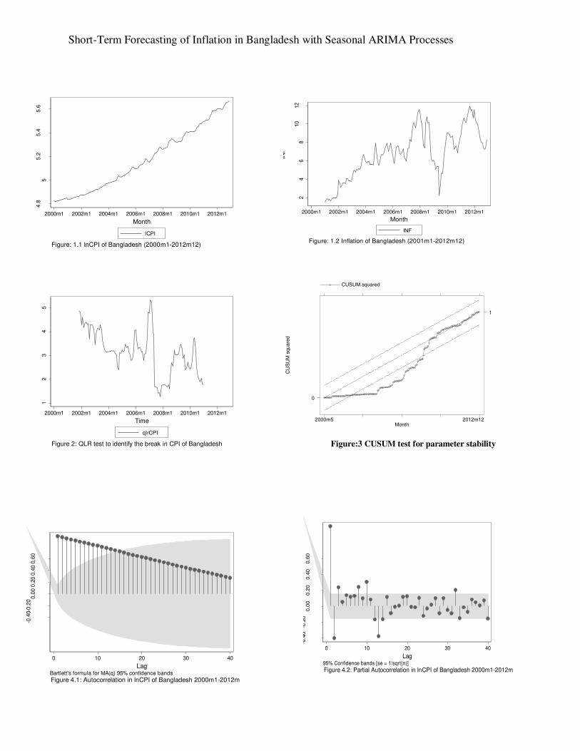
The graph of InCPI and inflation is depicted in figure 1.1 and 1.2 . From figure 1.2 it can be seen

that the inflation increased with a stable rate before 2007 and the dispersion of inflation was

larger after 2007. Figure 1.2 also provides visual evidence that the structural breaks can be

presumed in the year 2007 to 2010. In order to gather more detailed information, the study

performed more elaborate structural break test, such as, CUSUM test, the Quandt likelihood ratio

(QLR) test and Chow test to identify the the exact year and the corresponding month of breaks in

inflation series.3

In figure 3, CUSUM test result shows that from 2002 to 2007 cumulated sum of residuals lies

outside of the 95 percent confidence band. Hence, the null hypothesis of parameter stability of

CPI is rejected at the 5 percent significance level. In figure 2, the Quandt likelihood ratio (QLR)

test represents the exact date of break for CPI series by using the likelihood ratio statistic (LR).

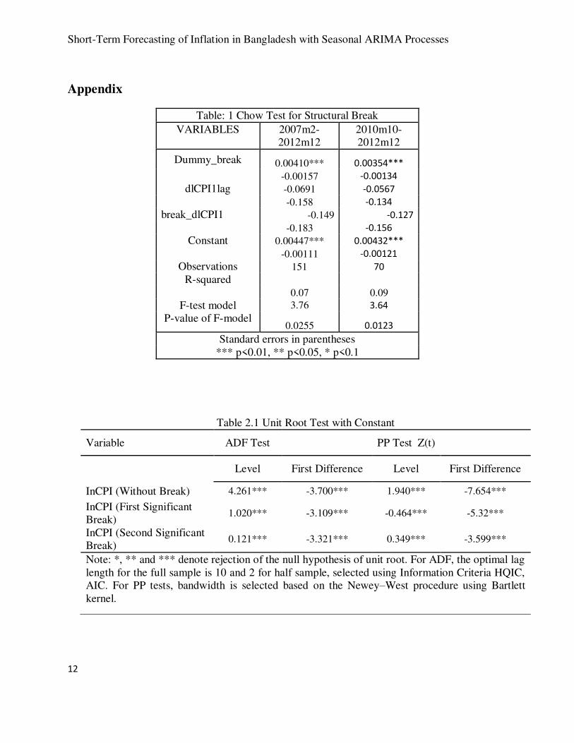
QRL ratio was 5.3153 in February 2007 and 4.35 in September 2009 respectively. Chow test also

confirms that the break of CPI series is significant in February 2007 and September 2010. Table

1 represents the results of the chow test for both sample periods, where the p - value is 0.02 <

0.05 reject the null hypothesis that no break in CPI series.

Data and Methodology

The study uses monthly consumer price indexes (CPI) starting from 2000 m1 to 2012 m12,

which comprises 156 observations. The monthly Consumer Price Indexes are collected from

series of official publications 'Economic Trend' of Bangladesh Bank. The estimation was

performed on a log series of base price index (1996=100). Considering the significant break in

CPI series, the sample divided into three periods, with significant break and without any break.

Finally, forecasting conducted up to December 2013 using best fitted models.

3 CUSUM measure the cumulative sum of the scaled residuals, which is generally used to test for parameter stability of a

regression.


5

SARIMA is a simple extension of ARIMA (Auto Regressive Integrated Moving Average) model

which is widely used to forecast seasonal time series data. In ARIMA (p, d, q) model, p shows

the number of autoregressive (AR) terms where AR predicts the series from its previous values

and q shows moving average (MA) terms where MA predicts the series from previous random

errors, or "shocks" and d is the number of non-seasonal difference. In SARIMA model by adding

seasonal components, ARIMA extends to (p, d, q) × (P, D, Q)s, where p and q are the order for

the non-seasonal AR and MA components and P and Q are the order of the seasonal AR and

MA components. D and d are the order of differencing for the seasonal and non-seasonal

respectively. If a plot of the time series data suggests that the seasonal effect is proportional to

the mean of the series, then the seasonal effect is probably multiplicative and a multiplicative

SARIMA model may be appropriate (Box, Jenkins, and Reinsel, 2008). Now, the generalized

form of the multiplicative SARIMA model can be written as (Box et al., 2008; Cryer and Chan,

2008):

..................................................................(1)

Where,

.................................................(2)

............................................................(3)

Where,

represents white noise error (random shock) at period t.4

B represents backward shift operator.

S represent seasonal order.5

For example, the SARIMA (1, 0, 1) (1, 1, 1)12 model is a multiplicative model of the form:

................................(6)

Using the properties of operator B, it follows that:

4 White noise is a series of uncorrelated random variables with zero expectation and equal variance.

5 s = 4 for quarterly data and s =12 for monthly data.


6

In equation (1) SARIMA models are suitable for modelling time series that include seasonality

both changeable and deterministic. The presence or absence of deterministic seasonality in In

CPI series can be detected using following regression equation with dummy variables,

Where, , ,........ are seasonal dummy variables. This means that the SARIMA (1,1,1)

(1,0,1)12 specification in (a) can mean that seasonality series is deterministic.

The estimation of SARIMA model consists of three steps, namely: identification, estimation of

parameters and diagnostic checking. The identification stage involves checking the stationary

and identifies the seasonality of the data series. Stationary confirms the existence or nonexistence

of a unit root in the data series. Unit root shows whether a stochastic or a deterministic trend is

present in the series. There are several statistical tests used for testing the presence of a unit root

in a series such as Augmented Dickey- Fuller (ADF) test and Phillips–Perron (PP) test (1988).6 If

the original series is not stationary then first difference will be appropriate to transform the series

into stationary. Further, the graphical presentation of time series can also confirm the stationary

and seasonality of the data series.

The next step in model identification stage is to determine the order of the model which is AR,

MA, SAR and SMA terms. The sample autocorrelation function (ACF) and partial

autocorrelation function (PACF) plot is often used to determine the order of the stationary series.

The ACF gives the information about covariance between past realizations. PACF helps to

determine the appropriate lags p in an AR (p) model. Particularly, an AR-process has a

(exponentially) declining ACF and spikes for the PACF and an MA-process has spikes in the

6 The study uses both tests but eventually focus on PP test results because PP tests ignore any serial correlation in a

time series data. Besides, the advantage of PP test over ADF test is that the user does not need to specify the lag

length for PP test.


7

ACF and (exponentially) declining PACF, where the number of significant spikes suggests the

order of the model.

Although the ACF and PACF assist in determining the order of the model but that information

are not adequate for modeling SARIMA. In this case several models with different order can be

considered to estimate the inflation series. But the final model will be selected based on a penalty

function statistics such as Akaike Information Criterion (AIC) or Bayesian Information Criterion

(BIC).7 The AIC and BIC are a measure of the goodness of fit of an estimated statistical model.

Given a data set, the study ranked several competing models according to their AIC or BIC. The

model with the lowest information criterion value will be the best. In the general case, the AIC

and BIC take the form as shown below:

Where,

k: is the number of parameters in the statistical model.

L: is the maximized value of the likelihood function for the estimated model.

RSS: is the residual sum of squares of the estimated model.

The next step in SARIMA model is to estimate the parameters of the chosen model using the

method of maximum likelihood estimation (MLE). To satisfy ARIMA conditions, the absolute

value of the coefficient must be always less than unity.

After estimating the parameters, the last step is model diagnostics. At this stage the study will

determine the adequacy of the chosen model. These checks are usually based on the residuals of

the model. One assumption of the SARIMA model is that, the residuals of the model should be

white noise. When the residuals are white noise, then the ACF of the residuals is approximately

zero. If this assumption is not fulfilled then the different model must be searched to satisfy the

7 See Sakamoto et. al. (1986); Akaike (1974) and Schwarz (1978).


8

assumption. Several statistical tests such as Ljung- Box Q statistic and Shapiro normality test

also used to check for autocorrelation and normality among the residuals in the model.

If the model passed the entire diagnostic test, then it becomes adequate for forecasting. To

choose a final model for forecasting, the accuracy of the model must be higher than that of all the

competing models. The accuracy of each model can be checked to determine how the model

performed in terms of in-sample forecast. The study tested the quality of the obtained forecasts

against two standard measures: Mean Absolute Error (MAE) and Root Mean Squared Error

(RMSE), which were defined as follows. If are actual values and a

random variable x, then:

A model with a minimum of these statistics will be considered as the best for forecasting.

Results and Discussions

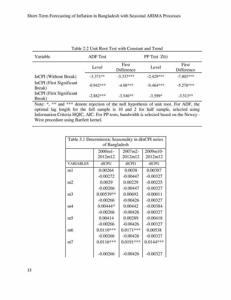
The statistical tests ADF and PP in Table 2.1 and 2.2 confirms the existence of unit root with

constant and constant with linear trend in InCPI which indicates that for all three samples, InCPI

series is not stationary at level. Considering the first non-seasonal differenced series, ADF and

PP tests confirm the non-existence of unit root with constant and constant with linear trend,

which indicate that the series is stationary at first difference i.e. InCPI data are integrated of

order (1).

Moreover, non stationarity of InCPI can also be confirmed from the sets of figure 4. The plots

illustrate the slow decay in the ACF of the InCPI series and very statistically significant spikes at

lag 1 of the PACF with marginal spikes at few other lags such as 2, 3, 8 and 10 for three samples.

Thus, looking at the sample ACF and PACF of InCPI, it is hard to identify any pure AR or MA

structure for SARIMA models. The sets of figure 4 also confirms that the InCPI is stationary at

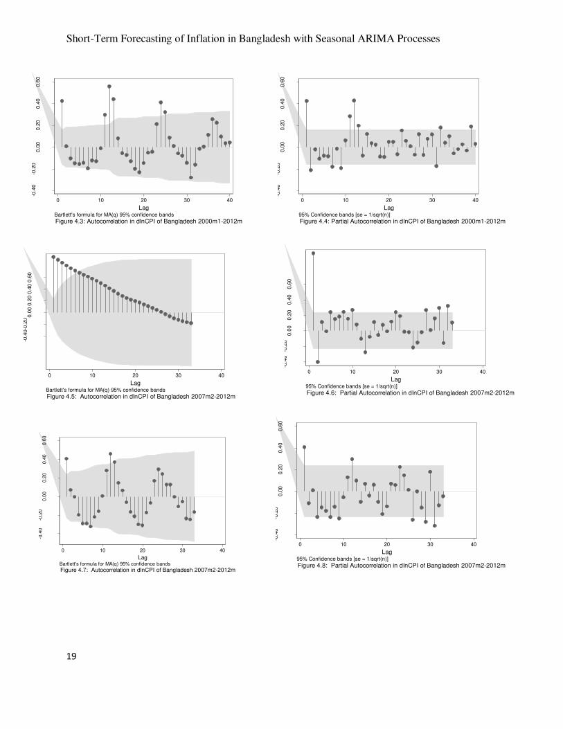
first difference. The sample ACF and PACF plot of dICPI shows the statistically significant

spike at lag 1 and 12, 24 for three samples, which indicating the strong seasonal variation in

InCPI series of Bangladesh.

In the identification stage, time series plot of ACF and PACF helps to determine the order of the

SARIMA models . For the first sample, considering first differenced of InCPI, figure 4.3 and 4.4


9

shows that ACF tails of at lag 1 and the PACF spike at lag 1, suggesting that p=1 and q=1

describe the non-seasonal autoregressive process and moving average for CPI series. Also

looking at the seasonal lags, ACF and the PACF both spike at lag 1 and lag 12, suggesting that a

seasonal moving average (SMA) and autoregressive process (SAR) need to include in the model.

Hence, ARIMA (1, 1, 1) (1, 0, 1)12, may perhaps the possible model for forecasting inflation of

Bangladesh using full sample 2000m1 to 2012m12. For the second sample, considering first

differenced of InCPI, figure 4.7 and 4.8 shows that ACF tails of at lag 1 and the PACF spike at

lag 1, suggesting that p=1 and q=1 describe the non-seasonal autoregressive process and moving

average for CPI series. To identify the seasonal lags, ACF and the PACF both spike at lag 1 and

lag 12, suggesting that a seasonal moving average (SMA) and autoregressive process (SAR)

need to include in the model. Hence, ARIMA (1, 1, 1) (1, 0, 1)12, may perhaps the possible

model for forecasting inflation of Bangladesh using second sample data from 2007m9 to

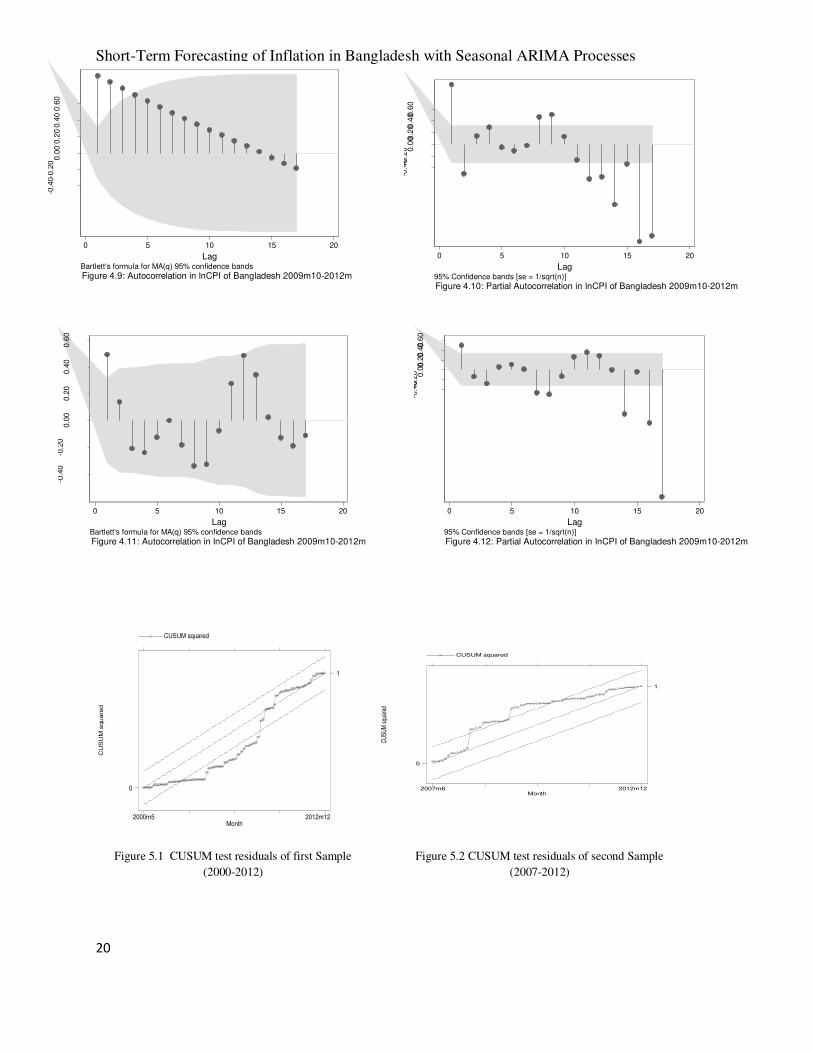
2012m12. Following the same way, considering first differenced of InCPI, figure 4.11 and 4.12

shows that ACF tails of at lag 1 and the PACF spike at lag 1, suggesting that p=1 and q=1

describe the non-seasonal autoregressive process and moving average for CPI series. The figures

also suggest that, ACF and the PACF both spike at lag 1 and lag 12, confirms that a seasonal

moving average (SMA) and autoregressive process (SAR) need to include in the model. Thus,

ARIMA (1, 1, 1) (1, 0, 1)12, may perhaps the possible model for forecasting inflation of

Bangladesh using third sample data 2009m10 to 2012m12.

Seasonality in dlnCPI series also reveals using the seasonal dummy model. Table 3.1 represents

that the seasonality of dlnCPI is simply deterministic for all three samples. In order to keep the

seasonal effect in forecasted months, the study considers the the seasonal difference D=0.

Although the sample Autocorrelation function and Partial Autocorrelation function is assisting to

determine the order of the SARIMA models but this is just an idea about the possible structure of

AR, SAR, MA and SMA. It becomes necessary to build the model around the suggested order. In

this case several models with different order considered to choose the final models. The study

estimates the SARIMA model with the four possible structures of AR,SAR,MA and SMA.

Table 4.1 represents the models with their corresponding values of AIC and BIC. Among those

possible models, comparing their AIC and BIC and minimum forecast error RMSE, ARIMA

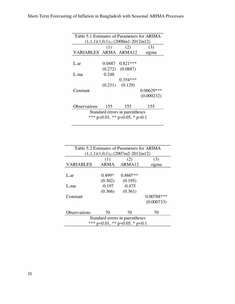
(1,1,1)(1,0,1)12 were chosen as the appropriate model for all three samples. Now, from derived

models, using the method maximum likelihood (MLE) the estimated parameters of the models

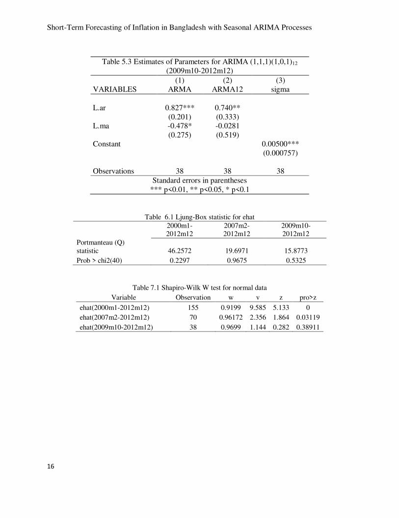
with their corresponding standard error is shown in the Table 5.1, 5.2 and 5.3. Based on 95%

confidence level seasonal AR and MA coefficients of the ARIMA (1, 1, 1) (1, 0, 1)12 models are

significantly different from zero for full sample and seasonal MA terms are significant for

second and third samples.


10

After estimate the model, the next step was diagnosed the model to see how well it fits the data.

One of the assumptions of ARIMA model is that, for being a good model, the residuals must

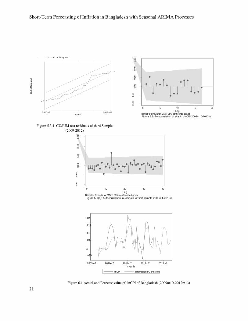
follow a white noise process. Fig 5.1(a) shows that for the first sample, ACF of the residuals are

not white noise, there was a significant spike at lag 12 of the residuals. Fig 5.3 shows that for the

third sample, ACF of the residuals are white noise, there was no significant spike in residuals.

Furthermore, the p-values for the Ljung-Box statistic in table 6.1 clearly exceeds 5% of all large

orders, indicating that the all three models were adequate for representing the data. But the

Shapiro - Wilk test in table 7.1 rejects the normality in residuals for first and second samples. In

figure 5.1 and 5.2 CUSUM test clearly illustrates that the residuals in first and second models

were not stable over the sample periods. Thus, for the first two samples, the selected model

ARIMA (1, 1, 1) (1, 0, 1)12 does not satisfy all the necessary assumptions for ARIMA model.

For the third sample, figure 5.3 shows that ACF of the residuals are white noise. The Shapiro -

Wilk test can not reject the normality in residuals for third sample. CUSUM test suggests that

residuals were stable over the sample periods September 2009 to December 2012. So the chosen

ARIMA (1, 1, 1) × (1, 0, 1)12 models for third sample was an adequate to estimate the CPI series

of Bangladesh .

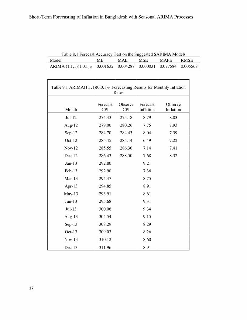
Finally, twelve months forecast conducted using ARIMA (1, 1, 1) × (1, 0, 1)12 model for third

sample. Table 8 presents the accuracy test for forecasted model. From the results, it can be seen

that, ARIMA (1, 1, 1) (1, 0, 1)12 models was adequate to be used to forecast the monthly

inflation rate of Bangladesh. Figure 6.1 shows the original CPI and the fitted values produced by

the obtained ARIMA (1, 1, 1) (1, 0, 1)12 model. The table 9.1 displays the original and the

forecasted value of CPI and inflation series of Bangladesh for next twelve months. Column 3 in

table 9.1 shows that the next peak of Bangladesh’s inflation is in the month of July 2013.

Conclusion

Following the Box, Jenkins, and Reinsel (1994) approach, Seasonal Autoregressive Integrated

Moving Average (SARIMA) was employed for forecasting monthly inflation rate of Bangladesh

for the coming months of January, 2013 to December 2013. To do so, several statistical tests

performed to identify the best fitted model for forecasting inflation series of Bangladesh.

structural break in CPI series identified the using CUSUM, QRL and Chow test. The result of

structural break tests shows that there were two significant breaks in CPI series of Bangladesh in

the year of 2007 and 2009. Hence, the study splits the sample in three different periods. Finally,

based on minimum AIC and BIC value, the best-fitted SARIMA models ARIMA(1,1,1)(1,0,1)12

were selected for all three samples. After the estimation of the parameters of selected model, a

series of diagnostic and forecast accuracy test were performed to check the validity of the

models. Only in third sample, residuals satisfied all the model assumptions. Hence, using CPI

data from September 2009 to December 2012, the study finds that ARIMA (1,1,1) (1,0,1)12

model was the best for forecasting inflation series of Bangladesh.


11

The forecasting results reveal an increasing pattern and high rates of inflation over the forecasted

period 2013. The results show that the next peak of inflation is in the month of July 2013.

Therefore, the study recommends that it is high time for the policy makers of the government of

Bangladesh and its central bank to come forward with more appropriate economic and monetary

policy in order to combat such increase in inflation rate which is yet to occur in the month of

July 2013.

The accuracy of inflation forecast is important because it will affect the quality of the policies

implemented based on this forecast. In this study, highest attempt has been made to forecast

inflation using best fitted ARIMA models. Nevertheless, the study recommends that future

research on this topic can utilize other time series models and then compare the performance of

the model used in this research in terms of forecast precision.

References

Aidan, M., Geoff, K. and Terry, Q. (1998). Forecasting Irish Inflation Using ARIMA Models.

CBI Technical Papers 3/RT/98:1-48, Central Bank and Financial Services Authority of Ireland.

Akaike, H.(1974). A New Look at the Statistical Model Identification. IEEE Transactions on

Automatic Controll 19 (6): 716–723.

Box, G. E. P., Jenkins, G. M., & Reinsel, G. C. (1994). Time series analysis. New Jersey:

Prentice Hall.

Dickey, D.A. & Fuller, W.A. (1981). Likelihood Ratio Statistics for Autoregressive Time Series

with a Unit Root, Econometrica, 49(4), 1057-1072.

Engle, R.F (2001). GARCH 101: The Use of ARCH/GARCH Models in Applied Econometrics,

Journal of Economic Perspectives, 15(4): 157-168

Junttila, J. (2001). Structural breaks, ARIMA Model and Finnish Inflation Forecasts,

International Journal of Forecasting, 17: 203–230

Meyler, A., G. Kenny and T. Quinn (1998): Forecasting Irish Inflation using ARIMA models,

Central Bank of Ireland, Technical Paper.

Pufnik, A. and Kunovac, D. (2006). Short-Term Forecasting of Inflation in Croatia with

Seasonal ARIMA Processes, Working Paper, W-16, Croatia National Bank.

Schulz, P.M. and Prinz, A. (2009). Forecasting Container Transshipment in Germany, Applied

Economics, 41(22): 2809-2815


12

Appendix

Table: 1 Chow Test for Structural Break

VARIABLES 2007m2-

2012m12

2010m10-

2012m12

Dummy_break 0.00410*** 0.00354***

-0.00157 -0.00134

dlCPI1lag -0.0691 -0.0567

-0.158 -0.134

break_dlCPI1 -0.149 -0.127

-0.183 -0.156

Constant 0.00447*** 0.00432***

-0.00111 -0.00121

Observations 151 70

R-squared

0.07 0.09

F-test model 3.76 3.64

P-value of F-model 0.0255 0.0123

Standard errors in parentheses

*** p<0.01, ** p<0.05, * p<0.1

Table 2.1 Unit Root Test with Constant

Variable ADF Test PP Test Z(t)

Level First Difference Level First Difference

InCPI (Without Break) 4.261*** -3.700*** 1.940*** -7.654***

InCPI (First Significant

Break) 1.020*** -3.109*** -0.464*** -5.32***

InCPI (Second Significant

Break) 0.121*** -3.321*** 0.349*** -3.599***

Note: *, ** and *** denote rejection of the null hypothesis of unit root. For ADF, the optimal lag

length for the full sample is 10 and 2 for half sample, selected using Information Criteria HQIC,

AIC. For PP tests, bandwidth is selected based on the Newey–West procedure using Bartlett

kernel.


13

Table 3.1 Deterministic Seasonality in dInCPI series

of Bangladesh

2000m1-

2012m12

2007m2-

2012m12

2009m10-

2012m12

VARIABLES dlCPI1 dlCPI1 dlCPI1

m1 0.00264 0.0038 0.00387

-0.00272 -0.00447 -0.00327

m2 0.0029 0.00229 -0.00225

-0.00266 -0.00447 -0.00327

m3 0.00539** 0.00692 -0.00011

-0.00266 -0.00426 -0.00327

m4 0.00444* 0.00442 -0.00384

-0.00266 -0.00426 -0.00327

m5 0.00414 0.00289 -0.00418

-0.00266 -0.00426 -0.00327

m6 0.0110*** 0.0171*** 0.00538

-0.00266 -0.00426 -0.00327

m7 0.0116*** 0.0191*** 0.0144***

-0.00266 -0.00426 -0.00327

Table 2.2 Unit Root Test with Constant and Trend

Variable ADF Test PP Test Z(t)

Level

First

Difference Level

First

Difference

InCPI (Without Break) -3.371** -5.337*** -2.429*** -7.803***


Break) -0.942*** -4.08*** -0.464*** -5.278***


Break) -2.882*** -3.546** -3.599* -3.513**

Note: *, ** and *** denote rejection of the null hypothesis of unit root. For ADF, the

optimal lag length for the full sample is 10 and 2 for half sample, selected using

Information Criteria HQIC, AIC. For PP tests, bandwidth is selected based on the Newey–West procedure using Bartlett kernel.


14

m8 0.0104*** 0.0139*** 0.0140***

-0.00266 -0.00426 -0.00327

m9 0.0131*** 0.0155*** 0.0122***

-0.00266 -0.00426 -0.00327

m10 0.00963*** 0.00937** 0.00135

-0.00266 -0.00426 -0.00327

m11 -0.000261 -0.000508 -0.00343

-0.00266 -0.00426 -0.00302

Constant -0.000862 -0.000897 0.00387*

-0.00188 -0.00301 -0.00214

Observations 155 70 38

R-squared 0.322 0.496 0.776

Standard errors in parentheses *** p<0.01, ** p<0.05, * p<0.1

Table 4.1 AIC , BIC and RMSE for the Suggested SARIMA Models (2000m1-2012m12)

Model AIC BIC RMSE

ARIMA(1,1,1)(1,0,1)12 -1114.431 -1099.214 .00632456

ARIMA(2,1,1)(1,0,1) 12 - -1114.457 - -1096.197 .00630079

ARIMA(1,1,0)(1,0,1) 12 -1115.738 -1103.565 .00634823

ARIMA(0,1,1)(1,0,1) 12 -1116.406 -1104.232 .00632456

Table 2.2: AIC , BIC and RMSE for the Suggested SARIMA Models (2007m2-2012m12)

Model AIC BIC RMSE

ARIMA(1,1,1)(1,0,1)12 -462.7233 -451.4808 .00843208

ARIMA(2,1,1)(1,0,1) 12 -461.7865 -450.3562 .00859878

ARIMA(1,1,0)(1,0,1) 12 -464.6042 -455.6102 .00845577

ARIMA(0,1,1)(1,0,1) 12 -464.2455 -455.2516 .00850882

Table 2.3: AIC , BIC and RMSE for the Suggested SARIMA Models (2009m10-2012m12)

Model AIC BIC RMSE

ARIMA(1,1,1)(1,0,1)12 -275.2109 -267.023 .00556776

ARIMA(2,1,1)(1,0,1) 12 -267.769 -259.5811 .00618061

ARIMA(1,1,0)(1,0,1) 12 -274.2488 -267.6984 .00575326

ARIMA(0,1,1)(1,0,1) 12 -270.069 -263.5186 .00627694


15

Table 5.1 Estimates of Parameters for ARIMA

(1,1,1)(1,0,1)12 (2000m1-2012m12)

(1) (2) (3)

VARIABLES ARMA ARMA12 sigma

L.ar 0.0487 0.821***

(0.272) (0.0887)

L.ma 0.248 -

0.354***

(0.231) (0.129)

Constant 0.00629***

(0.000232)



*** p<0.01, ** p<0.05, * p<0.1

Table 5.2 Estimates of Parameters for ARIMA

(1,1,1)(1,0,1)12 (2007m2-2012m12)

(1) (2) (3)


L.ar 0.499* 0.860***

(0.302) (0.195)

L.ma -0.197 -0.475

(0.366) (0.361)

Constant 0.00788***

(0.000733)



*** p<0.01, ** p<0.05, * p<0.1


16

Table 5.3 Estimates of Parameters for ARIMA (1,1,1)(1,0,1)12

(2009m10-2012m12)

(1) (2) (3)


L.ar 0.827*** 0.740**

(0.201) (0.333)

L.ma -0.478* -0.0281

(0.275) (0.519)

Constant 0.00500***

(0.000757)



*** p<0.01, ** p<0.05, * p<0.1

Table 6.1 Ljung-Box statistic for ehat

2000m1-2012m12

2007m2-2012m12

2009m10-2012m12

Portmanteau (Q)

statistic 46.2572 19.6971 15.8773

Prob > chi2(40) 0.2297 0.9675 0.5325

Table 7.1 Shapiro-Wilk W test for normal data

Variable Observation w v z pro>z

ehat(2000m1-2012m12) 155 0.9199 9.585 5.133 0

ehat(2007m2-2012m12) 70 0.96172 2.356 1.864 0.03119

ehat(2009m10-2012m12) 38 0.9699 1.144 0.282 0.38911


17

Table 8.1 Forecast Accuracy Test on the Suggested SARIMA Models

Model ME MAE MSE MAPE RMSE

ARIMA (1,1,1)(1,0,1)12 0.001632 0.004287 0.000031 0.077584 0.005568

Table 9.1 ARIMA(1,1,1)(0,0,1)12 Forecasting Results for Monthly Inflation

Rates

Month

Forecast

CPI

Observe

CPI

Forecast

Inflation

Observe

Inflation

Jul-12 274.43 275.18 8.79 8.03

Aug-12 279.00 280.26 7.75 7.93

Sep-12 284.70 284.43 8.04 7.39

Oct-12 285.45 285.14 6.49 7.22

Nov-12 285.55 286.30 7.14 7.41

Dec-12 286.43 288.50 7.68 8.32

Jan-13 292.80

9.21

Feb-13 292.90

7.36

Mar-13 294.47

8.75

Apr-13 294.85

8.91

May-13 293.91

8.61

Jun-13 295.68

9.31

Jul-13 300.06

9.34

Aug-13 304.54

9.15

Sep-13 308.29

8.29

Oct-13 309.03

8.26

Nov-13 310.12

8.60

Dec-13 311.96

8.91


18

12

34

5

2000m1 2002m1 2004m1 2006m1 2008m1 2010m1 2012m1

Time

qlrCPI

Figure 2: QLR test to identify the break in CPI of Bangladesh

CU

SU

M s

quare

d

Month

CUSUM squared

2000m5 2012m12

0

1

-0.4

0-0.2

00.0

00.2

00.4

00.6

0

0 10 20 30 40

LagBartlett's formula for MA(q) 95% confidence bands

Figure 4.1: Autocorrelation in lnCPI of Bangladesh 2000m1-2012m

Figure:3 CUSUM test for parameter stability

-0.4

0-0

.20

0.0

00.2

00.4

00.6

0

0 10 20 30 40

Lag95% Confidence bands [se = 1/sqrt(n)]

Figure 4.2: Partial Autocorrelation in lnCPI of Bangladesh 2000m1-2012m

4.8

55.2

5.4

5.6

2000m1 2002m1 2004m1 2006m1 2008m1 2010m1 2012m1

Month

lCPI

Figure: 1.1 lnCPI of Bangladesh (2000m1-2012m12)

24

68

10

12

INF

2000m1 2002m1 2004m1 2006m1 2008m1 2010m1 2012m1

Month

INF

Figure: 1.2 Inflation of Bangladesh (2001m1-2012m12)


19

-0.4

0-0

.20

0.0

00.2

00.4

00.6

0

0 10 20 30 40


Figure 4.3: Autocorrelation in dlnCPI of Bangladesh 2000m1-2012m

-0.4

0-0

.20

0.0

00.2

00.4

00.6

0

0 10 20 30 40


Figure 4.4: Partial Autocorrelation in dlnCPI of Bangladesh 2000m1-2012m

-0.4

0-0

.20

0.0

00.2

00.4

00.6

0

0 10 20 30 40



-0.4

0-0

.20

0.0

00.2

00.4

00.6

0

0 10 20 30 40



-0.4

0-0

.20

0.0

00.2

00.4

00.6

0

0 10 20 30 40



-0.4

0-0

.20

0.0

00.2

00.4

00.6

0

0 10 20 30 40




20

CU

SU

M s

quar

ed

Month

CUSUM squared

2007m6 2012m12

0

1

-0.4

0-0.2

00.0

00.2

00.4

00.6

0

0 5 10 15 20



-0.4

0-0.2

0 0.0

00.2

00.4

00.6

0

0 5 10 15 20



-0.4

0-0

.20

0.0

00.2

00.4

00.6

0

0 5 10 15 20



-0.4

0-0.2

0 0.0

00.2

00.4

00.6

0

0 5 10 15 20



CU

SU

M s

quare

d

Month

CUSUM squared

2000m5 2012m12

0

1

Figure 5.1 CUSUM test residuals of first Sample

(2000-2012)

Figure 5.2 CUSUM test residuals of second Sample

(2007-2012)


21

-0.4

0-0

.20

0.0

00.2

00.4

00.6

0

0 5 10 15 20


Figure 5.3: Autocorrelation of ehat in dlnCPI 2009m10-2012m

-0.4

0-0

.20

0.0

00.2

00.4

00.6

0

0 10 20 30 40


Figure 5.1(a): Autocorrelation in residuls for first sample 2000m1-2012m

-.005

0

.005

.01

.015

.02

2009m7 2010m7 2011m7 2012m7 2013m7 month

dlCPI1 xb prediction, one-step

Figure 5.3.1 CUSUM test residuals of third Sample

(2009-2012)

CU

SU

M s

quare

d

month

CUSUM squared

2010m2 2012m12

0

1

Figure 6.1 Actual and Forecast value of lnCPI of Bangladesh (2009m10-2012m13)

Documents

Short-Term Forecasting of Inflation in Bangladesh with Seasonal