Embed Size (px)
Citation preview

Short-term Hydropower Scheduling - A Stochastic
Approach
Helga Kristine Lumb and Vivi Kristine Weiss
December 20, 2006


Preface
This paper is prepared as our Project Thesis at the Norwegian University of Scienceand Technology (NTNU) at the Department of Industrial Economics and TechnologyManagement. The work has been accomplished during the autumn semester 2006 andthe paper is a part of the course TIØ 4700 Finance and Accounting, Specialization.
We would specially like to thank our teaching supervisor, Associate Professor Stein-Erik Fleten for helpful assistance and constructive feedback. In addition we thank LarsHolmefjord at Statkraft AS for support, valuable data to our case study and interestingeld trip to a hydropower plant.
Trondheim, December 20, 2006
Helga Kristine Lumb Vivi Kristine Weiss
i


Abstract
The common practice among Norwegian hydropower producers is to use a deterministicapproach in the bidding into the day-ahead market. However, day-ahead market pricesand water inow to the reservoirs are uncertain also within a short time frame. Basedon this fact we propose a stochastic short-term bidding and scheduling model for a price-taking hydropower producer who participates in the Nordic electricity day-ahead market,Elspot. Bidding to the spot market and a simplied version of the unit commitmentproblem is modeled within the framework of a two-stage linear stochastic model andsolved as a deterministic equivalent. The objective is to maximize the revenues fromsales in the market. To substantiate the model, relevant aspects of the Nordic day-aheadmarket, hydropower scheduling, bidding and stochastic programming are illustrated.
A demonstration of the model is presented using data from a Norwegian hydropowerproducer. To represent the uncertainty, scenarios for price and inow are generatedusing a moment-matching scenario generation method. The model is run with sets ofscenarios consisting of respectively 1, 10, 100 and 250 scenarios. The preliminary resultsshow a slight improvement in the objective value when the model is run with increasingnumber of scenarios.
iii

Contents
Preface i
Abstract iii
1 Introduction 1
1.1 Background and Motivation . . . . . . . . . . . . . . . . . . . . . . . . . . 1
1.2 Structure of the Paper . . . . . . . . . . . . . . . . . . . . . . . . . . . . . 2
2 The Nordic Electricity Market 3
2.1 Nord Pool . . . . . . . . . . . . . . . . . . . . . . . . . . . . . . . . . . . . 3
2.1.1 Bidding Process at Nord Pool . . . . . . . . . . . . . . . . . . . . . 4
2.2 The Short-term Balancing Market . . . . . . . . . . . . . . . . . . . . . . 5
3 Hydropower Scheduling 7
3.1 The Concept of Water Value . . . . . . . . . . . . . . . . . . . . . . . . . . 7
3.2 The Hydropower Scheduling Problem . . . . . . . . . . . . . . . . . . . . . 9
3.2.1 Medium- and Long-term Scheduling . . . . . . . . . . . . . . . . . 9
3.2.2 Short-term Scheduling . . . . . . . . . . . . . . . . . . . . . . . . . 10
4 Approaches to Bidding 15
4.1 Bidding in Practice . . . . . . . . . . . . . . . . . . . . . . . . . . . . . . . 15
4.2 Day-ahead Bidding in View of the Balancing Market . . . . . . . . . . . . 17
4.2.1 Day-ahead Bidding in View of the Balancing Market: Producer'sPerspective . . . . . . . . . . . . . . . . . . . . . . . . . . . . . . . 17
4.3 Strategic Bidding . . . . . . . . . . . . . . . . . . . . . . . . . . . . . . . . 21
5 Stochastic Programming 23
5.1 Introduction to Stochastic Programming . . . . . . . . . . . . . . . . . . . 23
5.1.1 Modeling . . . . . . . . . . . . . . . . . . . . . . . . . . . . . . . . 23
5.1.2 An Example of Stochastic Linear Programming . . . . . . . . . . . 24
5.2 Mathematical Formulation of Stochastic Programming . . . . . . . . . . . 26
5.2.1 General Formulation of the Stochastic Programming Model . . . . 26
5.2.2 Deterministic Equivalent . . . . . . . . . . . . . . . . . . . . . . . . 26
v
vi CONTENTS
5.2.3 Multi-stage Stochastic Programming . . . . . . . . . . . . . . . . . 27
5.3 Importance of Scenario Tree in Stochastic Programming . . . . . . . . . . 28
5.3.1 Scenario Tree . . . . . . . . . . . . . . . . . . . . . . . . . . . . . . 28
5.3.2 Measure of Quality in Scenario Trees . . . . . . . . . . . . . . . . . 28
5.4 Scenario Generation . . . . . . . . . . . . . . . . . . . . . . . . . . . . . . 31
5.4.1 Introduction . . . . . . . . . . . . . . . . . . . . . . . . . . . . . . . 31
5.4.2 A Heuristic for Moment-matching Scenario Generation . . . . . . . 31
5.5 Value of Stochastic Programming . . . . . . . . . . . . . . . . . . . . . . . 32
5.5.1 Introduction . . . . . . . . . . . . . . . . . . . . . . . . . . . . . . . 32
5.5.2 Comparing the Deterministic and Stochastic Objective Values . . . 32
5.5.3 The Value of the Stochastic Solution - VSS . . . . . . . . . . . . . 33
5.5.4 The Expected Value of Perfect Information - EVPI . . . . . . . . . 34
6 Case Study 35
6.1 Introduction . . . . . . . . . . . . . . . . . . . . . . . . . . . . . . . . . . . 35
6.1.1 The Case . . . . . . . . . . . . . . . . . . . . . . . . . . . . . . . . 36
6.2 Deterministic Model Formulation . . . . . . . . . . . . . . . . . . . . . . . 37
6.2.1 Choice of Time Horizon . . . . . . . . . . . . . . . . . . . . . . . . 37
6.2.2 Modeling the Bidding into Nord Pool . . . . . . . . . . . . . . . . . 37
6.2.3 Modeling the Power Stations . . . . . . . . . . . . . . . . . . . . . 39
6.2.4 Modeling the Water Value . . . . . . . . . . . . . . . . . . . . . . . 42
6.2.5 Modeling of Start and Stop Costs . . . . . . . . . . . . . . . . . . . 46
6.2.6 Objective Function . . . . . . . . . . . . . . . . . . . . . . . . . . . 48
6.3 The Stochastic Programming Model . . . . . . . . . . . . . . . . . . . . . 49
6.4 Scenario Generation . . . . . . . . . . . . . . . . . . . . . . . . . . . . . . 50
6.4.1 Application of the HKW Algorithm . . . . . . . . . . . . . . . . . . 50
6.4.2 Construction of Price Proles . . . . . . . . . . . . . . . . . . . . . 51
6.4.3 Some Results from the Scenario Generation . . . . . . . . . . . . . 52
6.5 Computational Results . . . . . . . . . . . . . . . . . . . . . . . . . . . . . 54
6.5.1 Initial Conditions . . . . . . . . . . . . . . . . . . . . . . . . . . . . 54
6.5.2 General Results . . . . . . . . . . . . . . . . . . . . . . . . . . . . . 54
6.5.3 Results from a Selected Set of Scenarios . . . . . . . . . . . . . . . 55
6.5.4 Stability Test . . . . . . . . . . . . . . . . . . . . . . . . . . . . . . 56
7 Conclusion and Future Work 60
7.1 Conclusion . . . . . . . . . . . . . . . . . . . . . . . . . . . . . . . . . . . . 60
7.2 Improving the Scenarios . . . . . . . . . . . . . . . . . . . . . . . . . . . . 60
7.3 Improving the model . . . . . . . . . . . . . . . . . . . . . . . . . . . . . . 61
7.4 Validation of the Model . . . . . . . . . . . . . . . . . . . . . . . . . . . . 62
A Input Data - Case Study 65
B CD-ROM 66

CONTENTS vii
C Xpress Programming Codes 67

Chapter 1
Introduction
1.1 Background and Motivation
The Nordic power producers are exposed to a volatile and competitive market when theyare to schedule production. In 2005 about 40% of the total concumption in the Nordicmarket were traded at the Nordic day-ahead market and the share is increasing (NVE2006). Hence, the sales of power into the day-ahead market constitutes a substantial partof the revenues for the producers. This makes the bidding into the day-ahead marketone of the most important tasks the power producers are faced with.
In the process of planning hydropower production, problems are usually categorizedaccording to their time horizon. The focus in this paper is on short-term hydropowerscheduling. The most important activities within the short-term scheduling include thebidding of the production into the electricity spot market a day in advance and theestablishment of a production plan which complies with the day-ahead commitmentsfrom the bidding. In these activities the future price and inow are important factors.
Future price and inow are stochastic variables in the short-term perspective. Neverthe-less, hydropower producers today use deterministic models in the short-term scheduling.Based on this we present a stochastic optimization model for short-term scheduling fora hydropower producer who only participates in the Nordic electricity spot market. Theobjective is to maximize prot from sales of power. We use the model presented in(Fleten & Kristoersen 2006) as a starting point.
We have accomplished a case study based on one of Statkraft ASs hydropower plants.Our motivation behind the case study is to see if a stochastic model performs better,i.e. have a higher objective value than the deterministic one. If so, one can argue thatthe stochastic model provides better support in the day-ahead bidding. The topology ofthe plant is rather complex and simplications is necessary to construct a linear model.First a deterministic linear model is formulated where we regard the bidding into the
1

2 CHAPTER 1. INTRODUCTION
day-ahead market and a simplied version of the unit commitment suited for the case.The model is then extended into a two-stage stochastic linear model and solved as adeterministic equivalent. To account for uncertainty, scenarios of price and inow areconstructed applying a moment-matching scenario generation method from (Høyland,Kaut & Wallace 2003). The models were programmed in Xpress Version 1.6.2. and someresults from the demonstration of the model are presented in the paper.
1.2 Structure of the Paper
The structure of the paper is as follows; Chapter 2 is an introduction to the Nordicpower market. Further in chapter 3 the concept of hydropower scheduling is presented. Inchapter 4 we discuss approaches to bidding. Chapter 5 deals with stochastic optimizationand has the purpose of being a study of the topic of stochastic optimization. Finally inchapter 6 we introduce the case study which is based on one of the hydropower plantsbelonging to Statkraft AS. Chapter 7 states a conclusion and suggests some improvementsleft for future work.
Chapter 2
The Nordic Electricity Market
2.1 Nord Pool
Nord Pool ASA is the Nordic power exchange. It has developed from being solely aNorwegian power exchange to be a multinational exchange for electrical power. NordPool provides the population of Norway, Sweden, Denmark and Finland with supply ofelectrical power and optimal use of total system resources.
With the liberalization of the Norwegian power market in 1991, the power sector changedfrom having monopoly areas under governmental regulation to be a competitive andmarket oriented sector. This process later proceeded in the rest of the Nordic region. Asa cause of the liberalization the producers had to change their focus from reliable andcost-ecient energy supply to more prot oriented and competitive objectives (Fleten,Wallace & Ziemba 2002). The liberalization of the market led to the need of a marketplace where a price could be set. Nord Pool oers a market for physical contracts anda market for nancial contracts. The market for physical contract is provided by NordPool Spot AS. Nord Pool also oers clearing services.
The market for physical contracts, Elspot, is an auction-based day-ahead market whereelectrical power contracts are traded for each hour the following day. Elspot providesan eective system for letting supply and demand set the market price, and it gives theparticipants the possibility to balance their portfolios of power contracts close to real-time load. Nevertheless, the time span between the day's Elspot auction and the actualdelivery hour of the concluded contracts is 36 hours at the most. As consumption andproduction situations change, a market player may nd a need for trading during these36 hours. The Elbas market provides continuous power trading 24 hours a day, up to onehour prior to delivery. The Elbas market is only available in Eastern Denmark, Finlandand Sweden. Since the purpose of this paper is to present a short-term scheduling modelfor a Norwegian hydropower producer, the Elbas market would not be treated further.
3

4 CHAPTER 2. THE NORDIC ELECTRICITY MARKET
There are four types of bids available at Elspot; hourly bids, block bids, exible hourlybids and linked block bids. In an hourly bid the participants submit how much they arewilling to buy or sell at a given price for every 24 hour starting at 00.00 the followingday. Flexible hourly bids are only sales bids for one single hour with a xed price andvolume. When bidding, a lower price limit and a volume is stated. The exible bidwill be accepted in the hour with the highest price. Block bid is an aggregated bid forminimum four consecutive hours with a xed price and volume. Linked block bids consistof a main block bid and a dependent block bid. If the main block is accepted, then thedependent block bid is also considered (NordPool 2004).
2.1.1 Bidding Process at Nord Pool
The participants at Elspot submit sales- and purchase bids for every hour of the followingday of operation. The bidding is done under uncertainty since the system price is notyet known. Because of the uncertainty, the bidding process is a dicult task. We willlater discuss this topic thoroughly.
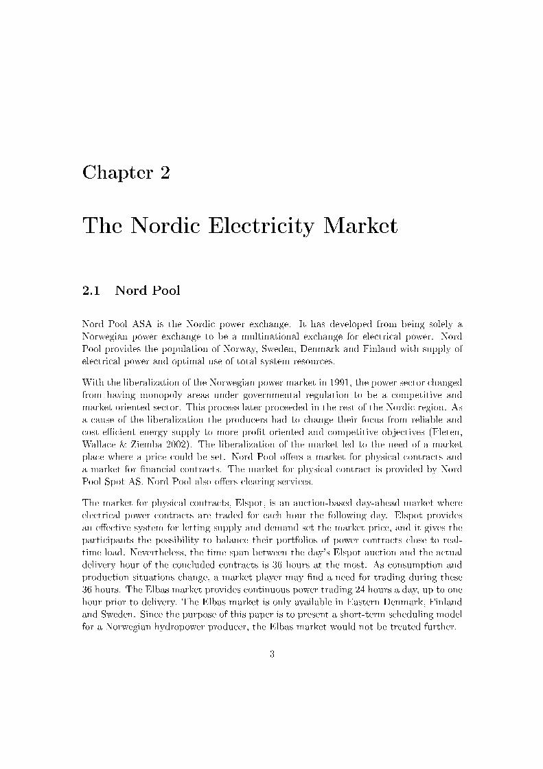
All the participants deliver their bids at the latest at 12.00. After the bidding Elspotcalculates the prices by aggregating the sales- and purchase-curves for every hour the fol-lowing day from the hourly bid curves. The spot prices are determined by the intersection-point between the resultant sales- and purchase-curves for every 24 hours the followingday (See gur 2.1). An hourly sales bid is accepted as long as the bid price is equal orlower than the spot price. The opposite is true for the purchase bids. Sales block bids areaccepted when the average spot price for the block period is equal or lower than the givenblock bid price. Again the opposite is true for purchase bids. Dependent linked blockbids are accepted under the same rules as regular block bids, but since linked block bidsare dependent of each other, the main block bid has to be accepted before the dependentone is considered. Flexibly hourly bids are not given for a specic hour, but are acceptedin the hour with the highest spot price given that the bid price is lower. The systemprice for a given day is an average over the 24 spot prices within that day.
If there are congestions in the grid, separate area prices will be established. In thefollowing we will assume that there are no dierent area prices, hence the spot pricesare the only prices in the whole Nordic area. The calculation of the spot prices arecompleted at the latest at 13.30. The spot prices and the belonging volume are thenpublished. All parties are notied how much volume they are obligated to dispatch. Alltransactions are handled at the spot price, and the accepted contracted volume, not themetered volume, decides the nancial settlements. If the metered volume diers from thecontracted volume, imbalances arise. This will be handled by the short-term balancingmarket (NordPool 2006).
2.2. THE SHORT-TERM BALANCING MARKET 5
Figure 2.1: Calculation of the spot price
2.2 The Short-term Balancing Market
The special feature of electricity is that it can not be stored in substantial part, and henceit has to be generated and consumed at the same time. We need a system that handlesthe imbalances between load and generation, such that the generation always equals theload. This is the objective of the short-term balancing market. The transmission systemoperators (TSOs) are responsible for this balancing within each country. The TSOs inthe Nordic countries cooperate to focus on the real time balance of the overall Nordicgrid. Statnett is the Norwegian system operator, and is responsible for the regulatingpower in Norway.
The participants in the balancing market submit their bids to the transmission systemoperator after the Elspot marked has closed, at the latest at 19.30. Balancing bids aredivided in two; bids for upward- and downward regulation. Bids for upward regulation arebids for increased generation or decreased consumption, where the participants submithow much they require for increasing generation or decreasing consumption for a speciedvolume. Bids for downward regulation signal how much they are willing to pay to decreasegeneration or increase consumption.
The TSO sorts each bid according to price for every hour during the day. In case ofupward regulation, there is a power decit in the market. The TSO therefore has toactivate the power reserves by informing the participants with the accepted bids fromthe balancing market. The accepted bids are chosen according to the ascending price, andthe last call-upon unit sets the price for upward regulation. For downward regulation thebids are accepted according to descending prices. In addition, spatial aspects are takeninto account. For example, in the case of upward regulation within a area the TSO callsa local generator to increase generation.

6 CHAPTER 2. THE NORDIC ELECTRICITY MARKET
There are dierent practices within the Nordic countries regarding how the imbalances arepriced. In Norway there is only one price for every hour in every price area. The nancialsettlements take place after real time regulation. The participants receive payment forpositive imbalances, and are charged for negative imbalances. Positive imbalance for aproducer is when he has generated more than he was obligated to in contracts at Elspotor in other physical contracts. A consumer will have positive imbalances when he hasconsumed less than the volume in the contracts. The volumes traded in the balancingmarket are often of insignicant quantity compared to the spot market. Hence, we willonly focus on the bidding in the spot market and not include the balancing market inthe short-term stochastic model presented later.
Chapter 3
Hydropower Scheduling
3.1 The Concept of Water Value
Water is the" fuel" in a hydropower plant. To be able to optimize the production it isnecessary to set a value on the water stored in the reservoirs. Even though water is forfree, it has a value given that it is a scarce resource and one is free to decide whether toproduce today or to store it for later production.
The water value is often referred to as the marginal operating costs of the power plant. Inreality, the water value is a function of the future development of the power market andthe inow. It should be noted that it is a complicated connection between the parametersthat aect the water value. Load and price are closely linked to one another. A high loadnecessarily results in a high price in a competitive market. This again gives an incentiveto discharge a considerable amount of water given that the market price is higher thanthe present water value of the reservoir. The discharge level in combination with theinow decides the reservoir level, which again inuences the water value. For instance ifthere is a small amount of water left in the reservoirs, the water will have a high valuesince the "fuel" is a scarce resource. In the opposite case, lets say the reservoir is nearlyfull, then there is a chance that the water ows over and becomes worthless since it willnever contribute to any production. In addition to reservoir level, the overall marketsituation aects the water value. Since all these variables are stochastic, we express thewater value by the expected value of the marginal kWh that is stored in the reservoirs(Fosso & Gjengedal 2006).
If the purpose is to maximize prot, one should produce until the short-term marginalcost equals the price. This is illustrated in section 4.1. Thus, a producer who participatesin the day-ahead market would like to bid equal to his marginal cost curve. Hydropowerplants in general have a low operating cost, and the only considerably cost is linked tothe discharge of water. Therefore, the marginal cost of operations equals the water value.This makes the water value an important aspect in the bidding process. In what follows,
7

8 CHAPTER 3. HYDROPOWER SCHEDULING
we will show that the water value equals marginal operational cost when minimizing totalcosts over a long time horizon. It should be noted that one may derive the same expressionwhen maximizing revenues. This is a more suitable approach in a deregulated market,but since the notion marginal cost is important in short-term production scheduling, costminimization will be used to derive the water value.
Let J(l, t) denote the expected total cost from period t until period T , where T is someremote future date and l is the reservoir level in period t. The costs of changing thewater level l is denoted Λ(l, T ) and is equal to the value of the water in the reservoirat period t, minus the value of the water in the reservoir at period T . In addition tothis cost, the expected total cost also consists of the sum of all operating cost, L(l, w, i)within a period i from t to T . The operating cost within a period i is dependent on thereservoir level l and the discharge of energy, w.
J(l, t) = Λ(l, T ) +T∑
i=t
L(l, w, i) = L(l, w, t) + J(l, t + 1) (3.1)
Equation (3.1) allude that the expected total costs from period t until T equal the sumof the operating cost in period t and the expected total costs from period t + 1 untilT . Optimal disposal of the water in period t is achieved when the expected total costs,J(l, t) are minimized in consideration to the energy disposal, w.
minw
J = minwL(l, w, t) + J(l, t + 1) (3.2)
⇒ dJ
dw= 0 (3.3)
δJ
δw=
δL
δwt+
δJ
δlt+1∗ δlt+1
δwt=
δL
δwt+
δJ
δlt+1∗ (−1) = 0 (3.4)
It should be noted from equation (3.4) that the marginal change in the reservoir levelcaused by a marginal change in the energy discharge in the anterior period is equal to−1.
Optimal strategy for period t can now be derived as
δL
δwt=
δJ
δlt+1(3.5)
The left side of the equation (3.5) equals the marginal operating costs. The right sideequals the expected total costs derived regarding to the reservoir level, which per deni-tion is the water value at time t + 1. Thus, the optimal strategy is to produce when theprice is higher than the water value.
3.2. THE HYDROPOWER SCHEDULING PROBLEM 9
The water value in period t is equal to the water value in period t + 1, given that theoptimal production strategy described above is applied in period t. When calculatingthe water value in period t one therefore needs the water value in the subsequent period.The calculation of water values is done using long-term models. One way to calculatethe water values is to choose the end of the planning horizon T such that it coincideswith a point in time where the water value is known. For instance when the snow meltis at its highest and ooding appear, one knows that the water value equals zero. Thisresult can be used to calculate backward until present period t is reached, for exampleusing a stochastic dynamic programming model.
3.2 The Hydropower Scheduling Problem
3.2.1 Medium- and Long-term Scheduling
The hydropower production scheduling is because of its complexity, decomposed intoa long-, medium- and short-term problem, each being solved by suitable models andsolution techniques (Flatabø, Fosso, Haugstad & Mo 2002).
The goal of the long-term production planning is to maximize the market value of thewater resources. The long-term production planning seeks to analyse the long-term uc-tuations in price and inow and by this nd an optimal strategy for the hydropoweroperations in the long run perspective. The modeling of the production is often sim-plied by aggregating the reservoirs into one equivalent reservoir. Stochastic dynamicprogramming can be applied to predict the water values from present time up to a pointin time in the future (Fleten et al. 2002). In this calculation price and inow prognosesprovide important input. Output from the long-term planning which among other fac-tors are the water values derived in equation (3.5), is further used as boundary conditionin the medium-term production planning. The medium-term model has an increasingdetail level and serve as a link between the long-term model and the short-term model(Fosso, Haugstad & Mo 2006).
SINTEF Energy Research has developed a model for long-term scheduling purpose, theEMPS model. This model is widely used in the Nordic areas. Within this model thewhole market including all the producers are considered. The EMPS model describesproduction, consumption and transmission within the Nordic and adjacent areas. Foreach sub area in the market the model gives an indication of the long-term situation ofthe water values, reservoir level, generation, sales and purchase of spot power. Importantinput in the model are load, thermal generation costs, and initial reservoir level (Flatabøet al. 2002).

10 CHAPTER 3. HYDROPOWER SCHEDULING
3.2.2 Short-term Scheduling
Short-term hydropower scheduling primarily deals with the physical operations of thepower plant within a time horizon of a day up to a week, depending on the coupling to themedium-term model, and with a time resolution of up to one hour (Fleten & Kristoersen2006). The main activities in the short-term scheduling are to make decisions that buildup under the planning of the physical production and can be listed as follows
• The bidding of production into a power exchange one day before actual time, oftenreferred to as the day-ahead commitments.
• Set up a detailed production plan which meets the terms from the day-ahead bid-ding.
• The real-time balancing, i.e. the establishment of the bids for the short-term bal-ancing markets.
Figure 3.1: Time schedule
We present how the procedure of the short-term scheduling can be accomplished accord-ing to the deadlines at the Nordic power exchange. The rst task in the short-termscheduling is to prepare the submitting of bids to the power exchange for the day-aheadcommitments. The bids have to be submitted to the power exchange at 12.00 at thelatest. Next, after the spot price is published around 13.00, one has to establish a pro-duction plan that complies with the day-ahead commitments. Not all, but some of thepower producers participate in the short-term balancing market. The nal deadline forsubmitting bids to this market is at 19.30.
The day-ahead bidding in the spot market is completed before the bidding in the balanc-ing market has been accomplished (Fleten & Kristoersen 2006). From section 3.1 weknow that it is optimal to bid to the marginal costs of your production for every hour.As stressed earlier, this is the water value of the reservoirs. In the modeling of the short-term scheduling it is complicated to derive the water value from equation (3.5), thusalternative approaches to express the water value may be used. Later in section 6.2.4 analternative way to derive an expression of the water value is applied. This approach isbased on a method used in (Fleten & Kristoersen 2006).
To sum up, the main tasks in the short-term scheduling can be separated in two; Firstis the submitting of bids for the day-ahead production, second is the unit commitmentof production which meet the terms of the day-ahead bidding, i.e. the decision of how to

3.2. THE HYDROPOWER SCHEDULING PROBLEM 11
distribute the production between the dierent aggregates. The bidding to the balancingmarket will be handled in chapter 4. It should be noted that bidding and unit commit-ment are closely related to one another, mainly because of the water value. As stressedearlier, the bids are set according to the water values. The production plan of how muchto produce from each reservoir is determined according to each reservoirs water value.For example, one will obviously discharge from the reservoirs with the lowest water valuerst.
Decisions of how to utilize the water resources are based on prot maximization of theexpected revenues from power sales. The short-term scheduling problem is rather com-plex, thus to be able to carry out the bidding and the unit commitment in light of protmaximization, a detailed modeling of the physical system is essential. Since the biddingand the unit commitment are dependent on another, an optimal model would includeboth operations. In chapter 6 we present an optimization model for short-term schedul-ing which include both the bidding and a simplied version of the unit commitment.Further in this chapter we will concentrate on only the unit commitment problem. Inchapter 4 the bidding issue will be carefully discussed.
How to Model the Unit Commitment
At this stage in the short-term scheduling the spot price is known and the remainingtask is to make a production plan for the next day which is consistent with the acceptedbids. This task is often referred to as the hydropower unit commitment problem. Moreprecisely it is that of determining which turbines should be on and the levels at whichto generate in each turbine so as to meet the commitment made in the spot market(Philpott, Craddock & Waterer 2000).
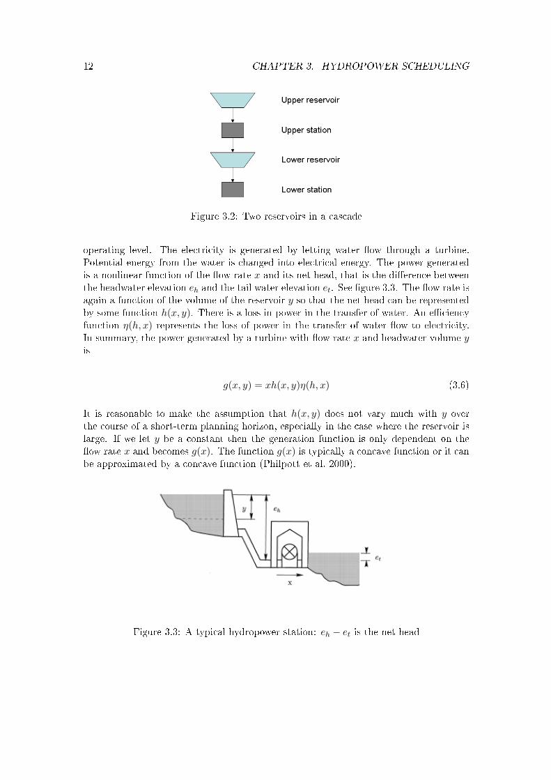
As stressed in the previous section the short-term scheduling is a rather complex task.The unit commitment problem requires that the detailing level of the physical system ishigh. In a model of the system, all the relevant details which aect the production mustbe taken into consideration. For example, hydropower plants may have quite complextopologies with several cascaded reservoirs or power plants in the same river system.The dierent reservoirs may have dierent storage capacity and signicant water traveltime. This has the eect that the decision in one time interval have strong impact onwhat is possible to do in later time steps (Belsnes, Honve & Fosso 2005). In cases wherethe reservoirs are linked in series, water release from an upper reservoir leads to waterinow in a lower reservoir. See gure 3.2. In addition, the start and stop costs makesthe decisions of production in one time step dependent on the decisions of the adjacenthours. The modeling of start and stop costs often requires binary variables expressingwhether each turbine is on or o. To avoid the computational eort by introducing binaryvariables one can model the start and stop in an alternative way which is introduced insection 6.2.5.
Each power plant may include several turbines which has a minimum and maximum
12 CHAPTER 3. HYDROPOWER SCHEDULING
Figure 3.2: Two reservoirs in a cascade
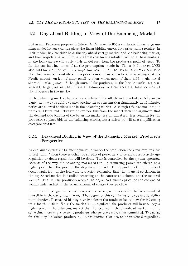
operating level. The electricity is generated by letting water ow through a turbine.Potential energy from the water is changed into electrical energy. The power generatedis a nonlinear function of the ow rate x and its net head, that is the dierence betweenthe headwater elevation eh and the tail water elevation et. See gure 3.3. The ow rate isagain a function of the volume of the reservoir y so that the net head can be representedby some function h(x, y). There is a loss in power in the transfer of water. An eciencyfunction η(h, x) represents the loss of power in the transfer of water ow to electricity.In summary, the power generated by a turbine with ow rate x and headwater volume yis
g(x, y) = xh(x, y)η(h, x) (3.6)
It is reasonable to make the assumption that h(x, y) does not vary much with y overthe course of a short-term planning horizon, especially in the case where the reservoir islarge. If we let y be a constant then the generation function is only dependent on theow rate x and becomes g(x). The function g(x) is typically a concave function or it canbe approximated by a concave function (Philpott et al. 2000).
Figure 3.3: A typical hydropower station: eh − et is the net head

3.2. THE HYDROPOWER SCHEDULING PROBLEM 13
It is dicult to consider all aspects of the physical system. For instance, in the case whena power plant has several owners the modeling is complicated. In addition there are oftenlegal requirements that have to be considered in the model. Hence, it is a challenge todevelop a model with a high enough detailing level.
Simulation and Optimization - Methods for solving the unit commitment
problem
Providing the utilities with optimal scheduling plans for each generator in the system isa dicult task. Existing approaches to unit commitment include both simulation andoptimization. A simulation is based on adjusting manual suggestions until a convincingplan is found. This approach is very user dependent and hence does not guarantee anoptimal plan. On the contrary, optimization represents a relatively impartial way ofmaking an optimal unit commitment (Fleten & Kristoersen 2006).
Further we will concentrate on the important aspects of an optimization model thatsatisfy the need for a high detailing level. Clearly, the objective in such a model shouldbe either prot maximization or cost minimization. In a deregulated market where theprice is set in a market clearing process at a power exchange, prot maximization isreasonable. Moreover, the cost in the objective function is related to the use of waterand the start and stop costs. The constraints constitute the modeling of the physicalsystem, as described in the previous section.
While price and inow are treated as stochastic variables in the long- and medium-termmodel, they are often treated as deterministic variables in the short-term scheduling.This is the praxis in spite of the fact that price and inow are subject to uncertaintyalso in the short-term perspective, at least in the case where both the bidding andthe unit commitment are included in the same optimization model. If the model onlyconcentrate on the unit commitment, one assumes that the market price is known inadvance i.e. the bidding has already been done and the market price is set. Nevertheless,the inow is still an uncertain variable in the unit commitment and should be modeledin a stochastic approach. The reason for the deterministic praxis is that a stochasticapproach is deemed to be computationally demanding because of the required detailinglevel. This is especially the case for cascaded reservoir systems (Flatabø et al. 2002).
Examples of Theory and Methodology of Short-term Scheduling in the Lit-
erature
In this section we will look at some approaches of how to model the short-term schedulingin the literature. A general model formulation of the short-term hydro scheduling ispresented by George, Read and Kerr (George, Read & Kerr 1995). This is a deterministicmodeling approach where integer variables are used to represent the number of turbinesoperating at each station along with piecewise linearization of the unit eciency curves.

14 CHAPTER 3. HYDROPOWER SCHEDULING
The objective is to maximize prot accrued from generation and the value of end of periodstorage of water in the reservoirs, less the costs of failing to meet generation targets andthe start and stop costs. No heuristic is applied to obtain faster solution time and themodel is solved with a standard IP solver.
Hreinsson (Hreinsson 1988) has made a deterministic optimization model with the pur-pose of nding the optimal short-term production scheduling of a hydropower system.More specically, the model optimizes the hourly power production by minimizing lossesin turbines and waterways, while maintaining production to meet load. The optimizationproblem is inherently formulated as a nonlinear mixed integer problem, but an algorithmhas been applied to solve the problem in two stages by linear programming. The modelis further simplied by letting the power production and the water resources be treatedseparately. In praxis, this means that the production is modeled without consideringany of the variables associated with water or reservoir content. With this simplicationthe number of variables is kept to a minimum and the problem can be solved with lesscomputational eort.
As mentioned before, the short-term modeling is often subject to a deterministic treat-ment in spite of its stochastic parameters. Philpott, Craddock and Waterer (Philpott etal. 2000) have regarded the uncertainty in the scheduling of daily hydro-electric genera-tion. With appropriate approximations the problem of determining what turbine unitsto commit in each half hour of the day can be formulated as a large mixed-integer linearprogramming problem. To be able to solve this stochastic problem they suggest usingan optimization-based heuristic.
SHOP (Short-term Hydro Operation Planning) is an example of a commercial modelingtool which is developed by SINTEF Energy Research. This is a deterministic linearprogramming model adjusted for solving complex hydropower scheduling problems. Asin the modeling approaches introduced above the power plant is modeled at unit level.Unlike the model of Philpott, Craddock and Waterer SHOP does not regard uncertaintyin the modeling formulation (Flatabø et al. 2002).
Chapter 4
Approaches to Bidding
4.1 Bidding in Practice
At the time of bidding the price is not yet known, thus the bidding is done under uncer-tainty. To reduce the uncertainty the planning of the bids will normally take place closeto the deadline because then the latest information can be used. For a prot maximizingproducer the philosophy behind the bidding should always be to maximize the expectedrevenues, i.e. to sell when the prices are high, and to buy when the prices are low. Thusthe important and dicult task is to nd out what a "high" and a "low" price is.
From microeconomic theory one knows that a producer who acts as price taker should tomaximize prot, produce until his short time marginal cost equals the price (Wangensteen2005). To see this, let C(w) be the producer's cost function, w the volume produced andρ the price set by the market. Then his prot π may be formulated as
π = w × ρ− C(w) (4.1)
Prot maximizing behavior implies
dπ
dw= ρ− dC(w)
dw= 0 (4.2)
which gives
ρ =dC(w)
dw(4.3)
Hence, to maximize prot the producers would bid equal to their marginal cost curve.From section 3.1 we know that the marginal costs equal the water values.
When constructing the bids there are several important issues the producer has to con-sider. For some power producers locked production is an issue, that is power they have
15
16 CHAPTER 4. APPROACHES TO BIDDING
to produce regardless of the price. Examples of this could be wind power or hydropowerfrom a river plant with no store possibilities. And even if there are store possibilitiesin the water chain, there are often legal requirements that state that the water ow hasto be at least at a given minimum level at all times because of ecological or estheticalconsiderations. Since they have to produce this power no matter what, the producersare willing to sell this power at any price. Thus the operator bids this locked volume toa price as low as zero, so that he is ensured a knockdown on this volume.
Then one has to consider how to bid the rest of the production. One way of constructingthese bids, which is used in practice, is to bid the water value at the best point ofproduction and at the maximum point of production for every generator. By doing this,the producer gets two price-volume points for every generator. The water value used inthe bidding process is usually found from long-term models, but some adjustments maybe done. For example the EMPS model, see section 3.2.1, could be run a few times perweek to get the water values given a long- and medium-term strategy. These weeklywater values would then be used as indicators of how the water value will be within thatgiven week. Since the market situation and inow vary from day to day, the weeklywater values may be modied on daily basis. The calculation of the daily water valuesare usually based on experience and analysis. Factors which indirectly inuence thedecisions are for example the expected weather forecast and the hydrological situationand the expected gas- and coal-price. The latter is important in the Nordic market sinceit consists mainly of hydropower and thermal production.
The decision of how much to bid for every hour is dependent from hour to hour. Asalready mentioned in section 3.2.2, the topology of the hydro system and the start andstop costs cause the production plan to be dependent on the consecutive hours. Atthe time when the bidding schemes are constructed, there already exists a schedulingplan for the remaining hours of the day. This is based on the commitment made in thespot market the day before. Since this scheduling plan eects the system state at thebeginning of the next bidding period, this too as to be considered when constructing thebids.
From the above discussion we see that in practice the process of making the bids is oftenbased on experience and the skills of the operator. In the literature we nd models whichhave a more theoretical approach and in the reminder of this chapter we will discuss twoarticles which both deal with bidding strategies. We illustrate two dierent approachesto the bidding problem. The rst one (Fleten & Pettersen 2005) addresses the possibilityof willingly bid too high or too low volumes in the day-ahead market to earn a prot inthe balancing market. The second one (Wen & David 2001) concerns the start and stopcosts issue.
4.2. DAY-AHEAD BIDDING IN VIEW OF THE BALANCING MARKET 17
4.2 Day-ahead Bidding in View of the Balancing Market
Fleten and Pettersen propose in (Fleten & Pettersen 2005) a stochastic linear program-ming model for constructing piecewise-linear bidding curves for a price-taking retailer. Intheir model they consider both the day-ahead energy market and the balancing market,and their objective is to minimize the total cost for the retailer from both these markets.In the following we will apply their model seen from the producer's point of view. Todo this one rst has to see if all the presumptions made in (Fleten & Pettersen 2005)also hold for the producer. One important assumption that Fleten and Pettersen do isthat they assume the retailers to be price takers. They argue for this by saying that theNordic market consists of many small retailers which none of them hold a substantialshare of market power. Although most of the producers in the Nordic market are con-siderably larger, we feel that this is an assumption one can accept at least for most ofthe producers in the market.
In the balancing market the producers behave dierently from the retailers. All partici-pants that have the ability to alter production or consumption signicantly on 15 minutesnotice are allowed to place bids in the balancing market. Although this also includes theretailers, Fleten and Pettersen do exclude this from the model with the argument thatthe demand side bidding of the balancing market is still immature. It is common for theproducers to place bids in the balancing market, nevertheless we will as a simplicationdisregard this fact.
4.2.1 Day-ahead Bidding in View of the Balancing Market: Producer's
Perspective
As explained earlier the balancing market balances the production and consumption closeto real time. When there is decit or surplus of power in a price area, respectively up-regulation or down-regulation will be done. This is controlled by the system operator.Because of the way the balancing market is run, up-regulating power are oered at ahigher price than the price in the day-ahead market. The opposite is true in hours ofdown-regulation. In the following discussion remember that the nancial settlement inthe day-ahead market is handled according to the contracted volume, not the meteredvolume. That is, the producers receive the day-ahead market price for the contractedvolume independent of the actual amount of energy they produce.
In the case of up-regulation consider a producer who generates less than he has committedhimself to in the day-ahead market. The reason for this can for instance be unavailabilityin production. Because of his negative imbalance the producer has to pay the balancingprice for the decit. Since the market is up-regulated the producer will have to pay ahigher price in the balancing market than he received in the day-ahead market. At thesame time there might be some producers who generate more than committed. The causefor this may be locked production, i.e. production that has to be produced regardless.
18 CHAPTER 4. APPROACHES TO BIDDING
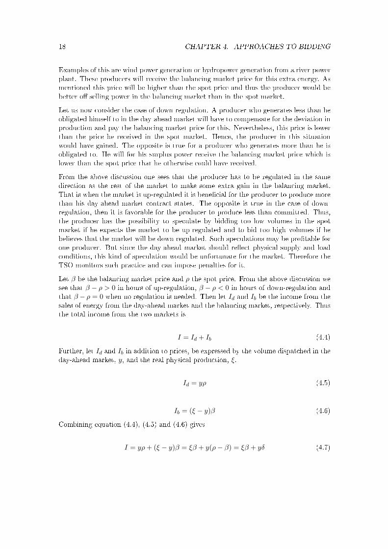
Examples of this are wind power generation or hydropower generation from a river powerplant. These producers will receive the balancing market price for this extra energy. Asmentioned this price will be higher than the spot price and thus the producer would bebetter o selling power in the balancing market than in the spot market.
Let us now consider the case of down-regulation. A producer who generates less than heobligated himself to in the day-ahead market will have to compensate for the deviation inproduction and pay the balancing market price for this. Nevertheless, this price is lowerthan the price he received in the spot market. Hence, the producer in this situationwould have gained. The opposite is true for a producer who generates more than he isobligated to. He will for his surplus power receive the balancing market price which islower than the spot price that he otherwise could have received.
From the above discussion one sees that the producer has to be regulated in the samedirection as the rest of the market to make some extra gain in the balancing market.That is when the market is up-regulated it is benecial for the producer to produce morethan his day-ahead market contract states. The opposite is true in the case of down-regulation, then it is favorable for the producer to produce less than committed. Thus,the producer has the possibility to speculate by bidding too low volumes in the spotmarket if he expects the market to be up-regulated and to bid too high volumes if hebelieves that the market will be down-regulated. Such speculations may be protable forone producer. But since the day-ahead market should reect physical supply and loadconditions, this kind of speculation would be unfortunate for the market. Therefore theTSO monitors such practice and can impose penalties for it.
Let β be the balancing market price and ρ the spot price. From the above discussion wesee that β − ρ > 0 in hours of up-regulation, β − ρ < 0 in hours of down-regulation andthat β − ρ = 0 when no regulation is needed. Then let Id and Ib be the income from thesales of energy from the day-ahead market and the balancing market, respectively. Thusthe total income from the two markets is
I = Id + Ib (4.4)
Further, let Id and Ib in addition to prices, be expressed by the volume dispatched in theday-ahead market, y, and the real physical production, ξ.
Id = yρ (4.5)
Ib = (ξ − y)β (4.6)
Combining equation (4.4), (4.5) and (4.6) gives
I = yρ + (ξ − y)β = ξβ + y(ρ− β) = ξβ + yδ (4.7)
4.2. DAY-AHEAD BIDDING IN VIEW OF THE BALANCING MARKET 19
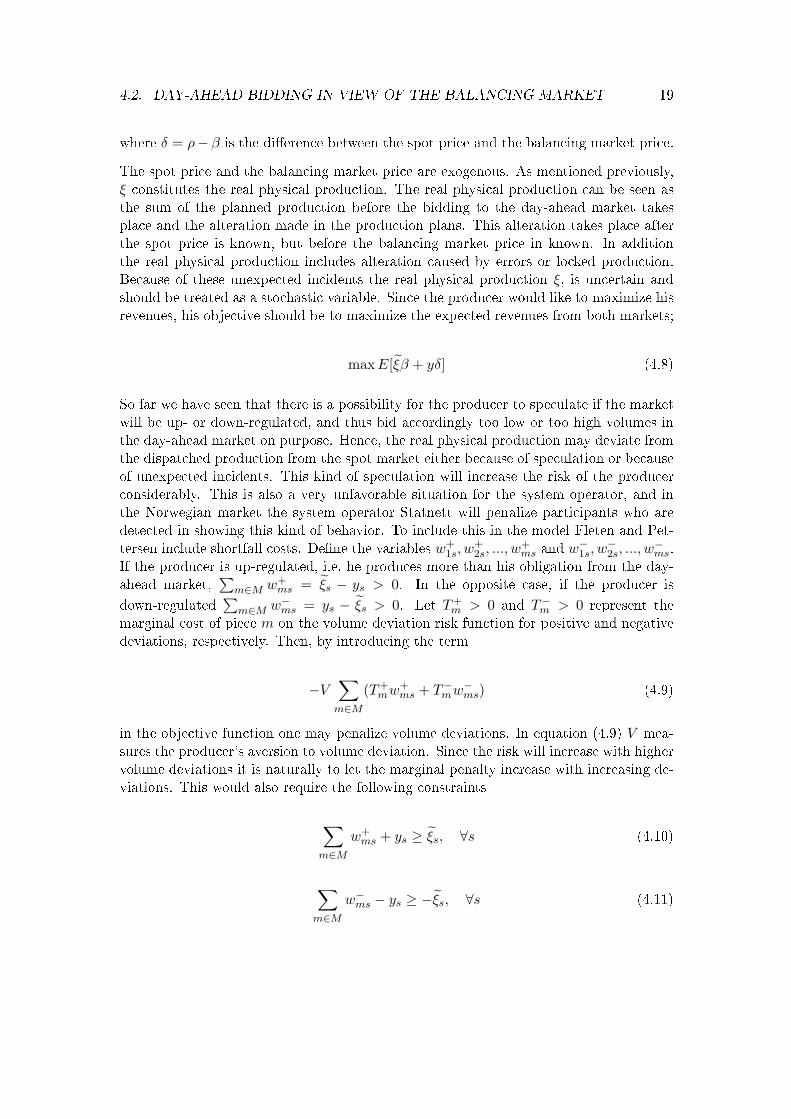
where δ = ρ− β is the dierence between the spot price and the balancing market price.
The spot price and the balancing market price are exogenous. As mentioned previously,ξ constitutes the real physical production. The real physical production can be seen asthe sum of the planned production before the bidding to the day-ahead market takesplace and the alteration made in the production plans. This alteration takes place afterthe spot price is known, but before the balancing market price in known. In additionthe real physical production includes alteration caused by errors or locked production.Because of these unexpected incidents the real physical production ξ, is uncertain andshould be treated as a stochastic variable. Since the producer would like to maximize hisrevenues, his objective should be to maximize the expected revenues from both markets;
max E[ξβ + yδ] (4.8)
So far we have seen that there is a possibility for the producer to speculate if the marketwill be up- or down-regulated, and thus bid accordingly too low or too high volumes inthe day-ahead market on purpose. Hence, the real physical production may deviate fromthe dispatched production from the spot market either because of speculation or becauseof unexpected incidents. This kind of speculation will increase the risk of the producerconsiderably. This is also a very unfavorable situation for the system operator, and inthe Norwegian market the system operator Statnett will penalize participants who aredetected in showing this kind of behavior. To include this in the model Fleten and Pet-tersen include shortfall costs. Dene the variables w+
1s, w+2s, ..., w
+ms and w−1s, w
−2s, ..., w
−ms.
If the producer is up-regulated, i.e. he produces more than his obligation from the day-ahead market,
∑m∈M w+
ms = ξs − ys > 0. In the opposite case, if the producer is
down-regulated∑
m∈M w−ms = ys − ξs > 0. Let T+m > 0 and T−m > 0 represent the
marginal cost of piece m on the volume deviation risk function for positive and negativedeviations, respectively. Then, by introducing the term
−V∑
m∈M
(T+mw+
ms + T−mw−ms) (4.9)
in the objective function one may penalize volume deviations. In equation (4.9) V mea-sures the producer's aversion to volume deviation. Since the risk will increase with highervolume deviations it is naturally to let the marginal penalty increase with increasing de-viations. This would also require the following constraints
∑m∈M
w+ms + ys ≥ ξs, ∀s (4.10)
∑m∈M
w−ms − ys ≥ −ξs, ∀s (4.11)
20 CHAPTER 4. APPROACHES TO BIDDING
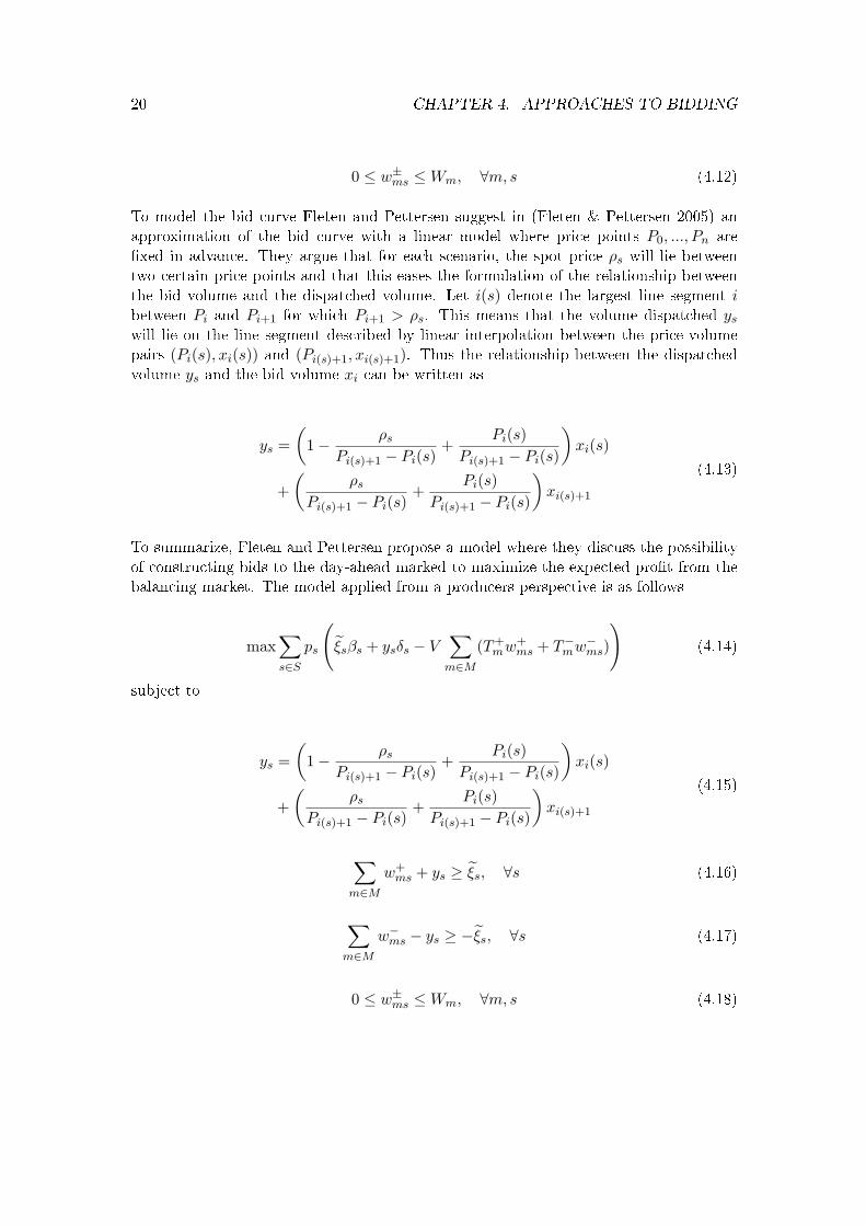
0 ≤ w±ms ≤ Wm, ∀m, s (4.12)
To model the bid curve Fleten and Pettersen suggest in (Fleten & Pettersen 2005) anapproximation of the bid curve with a linear model where price points P0, ..., Pn arexed in advance. They argue that for each scenario, the spot price ρs will lie betweentwo certain price points and that this eases the formulation of the relationship betweenthe bid volume and the dispatched volume. Let i(s) denote the largest line segment ibetween Pi and Pi+1 for which Pi+1 > ρs. This means that the volume dispatched ys
will lie on the line segment described by linear interpolation between the price-volumepairs (Pi(s), xi(s)) and (Pi(s)+1, xi(s)+1). Thus the relationship between the dispatchedvolume ys and the bid volume xi can be written as
ys =(
1− ρs
Pi(s)+1 − Pi(s)+
Pi(s)Pi(s)+1 − Pi(s)
)xi(s)
+(
ρs
Pi(s)+1 − Pi(s)+
Pi(s)Pi(s)+1 − Pi(s)
)xi(s)+1
(4.13)
To summarize, Fleten and Pettersen propose a model where they discuss the possibilityof constructing bids to the day-ahead marked to maximize the expected prot from thebalancing market. The model applied from a producers perspective is as follows
max∑s∈S
ps
(ξsβs + ysδs − V
∑m∈M
(T+mw+
ms + T−mw−ms)
)(4.14)
subject to
ys =(
1− ρs
Pi(s)+1 − Pi(s)+
Pi(s)Pi(s)+1 − Pi(s)
)xi(s)
+(
ρs
Pi(s)+1 − Pi(s)+
Pi(s)Pi(s)+1 − Pi(s)
)xi(s)+1
(4.15)
∑m∈M
w+ms + ys ≥ ξs, ∀s (4.16)
∑m∈M
w−ms − ys ≥ −ξs, ∀s (4.17)
0 ≤ w±ms ≤ Wm, ∀m, s (4.18)
4.3. STRATEGIC BIDDING 21
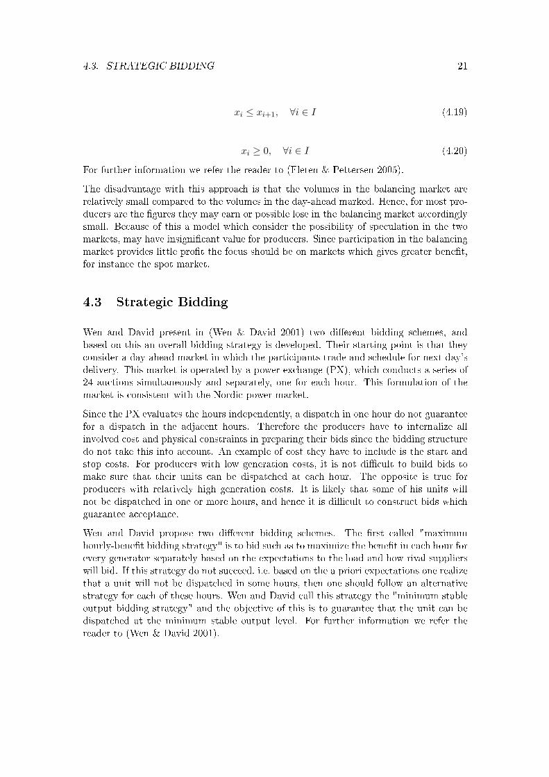
xi ≤ xi+1, ∀i ∈ I (4.19)
xi ≥ 0, ∀i ∈ I (4.20)
For further information we refer the reader to (Fleten & Pettersen 2005).
The disadvantage with this approach is that the volumes in the balancing market arerelatively small compared to the volumes in the day-ahead marked. Hence, for most pro-ducers are the gures they may earn or possible lose in the balancing market accordinglysmall. Because of this a model which consider the possibility of speculation in the twomarkets, may have insignicant value for producers. Since participation in the balancingmarket provides little prot the focus should be on markets which gives greater benet,for instance the spot market.
4.3 Strategic Bidding
Wen and David present in (Wen & David 2001) two dierent bidding schemes, andbased on this an overall bidding strategy is developed. Their starting point is that theyconsider a day-ahead market in which the participants trade and schedule for next day'sdelivery. This market is operated by a power exchange (PX), which conducts a series of24 auctions simultaneously and separately, one for each hour. This formulation of themarket is consistent with the Nordic power market.
Since the PX evaluates the hours independently, a dispatch in one hour do not guaranteefor a dispatch in the adjacent hours. Therefore the producers have to internalize allinvolved cost and physical constraints in preparing their bids since the bidding structuredo not take this into account. An example of cost they have to include is the start andstop costs. For producers with low generation costs, it is not dicult to build bids tomake sure that their units can be dispatched at each hour. The opposite is true forproducers with relatively high generation costs. It is likely that some of his units willnot be dispatched in one or more hours, and hence it is dicult to construct bids whichguarantee acceptance.
Wen and David propose two dierent bidding schemes. The rst called "maximumhourly-benet bidding strategy" is to bid such as to maximize the benet in each hour forevery generator separately based on the expectations to the load and how rival supplierswill bid. If this strategy do not succeed, i.e. based on the a priori expectations one realizethat a unit will not be dispatched in some hours, then one should follow an alternativestrategy for each of these hours. Wen and David call this strategy the "minimum stableoutput bidding strategy" and the objective of this is to guarantee that the unit can bedispatched at the minimum stable output level. For further information we refer thereader to (Wen & David 2001).

22 CHAPTER 4. APPROACHES TO BIDDING
The model presented in (Wen & David 2001) is especially suitable for producers with amarginal cost close to the market price. In the Nordic market, inow is the principalprice driver but the marginal cost levels of the thermal plants are also of high signicance(Tjøtta 2006). In periods with considerably inow and high reservoir levels the watervalue tends to be low. Hence, in such a situation the marginal cost level of the thermalproducers and the load set the price. This is true for all periods where the water valueis lower than the thermal marginal cost and this is the usual situation. If the tendencyis that the water values are high and at the same time the fuel costs of the thermalplants are low, then periods can arise where the marginal costs of the hydro producersare higher than the marginal costs of the thermal producers. In such a situation thehydropower production and the load set the price, and many of the hydropower producerswill therefore have marginal costs close to the market price.
From the discussion above we see that hydropower or thermal power production canset the price depending on which of them having the highest marginal costs. Although,the thermal power production usually have the highest generation costs and thereforeare probably most suited for applying such a model that Wen and David propose, wesee that the model in (Wen & David 2001) also can be relevant for hydro producers.In addition the consideration of start and stop costs are important for a hydropowerproducer. Since Wen and David's model reect this importance, the use of their modelfor a hydro producer can be justied also when the water value is much lower than themarket price.
Chapter 5
Stochastic Programming
5.1 Introduction to Stochastic Programming
5.1.1 Modeling
When investigating a natural system for instance a hydropower plant, one usually makes amodel which is applied to give the decision makers a better understanding and overviewof the system. This is done because the natural system is too complex, dicult orexpensive to study directly.
The accuracy of the model, i.e. how detailed and how close to the real world the modelis, does not necessarily measure the quality of the model. Instead one has to look at thepurpose of the model to nd the right degree of detailing level. As we saw in section 3.2a long-term model in production scheduling will usually be less detailed than a short-term production scheduling model where more work is done to make the model resemblethe real world. This does not mean that a short-term model is "better", it only showsthat these models serve dierent purposes. It is therefore important to remember that amodel is never a copy of the real world and that one can never mimic every aspects of asystem (Wallace 1999).
There are dierent ways to categorize dierent models. A common procedure is to splitmathematical programming problems into linear programming, nonlinear programming,networks ow, integer and combinatorial optimization and nally stochastic program-ming. Such classication can be confusing because it indicates that stochastic program-ming is dierent from linear programming in the same way as nonlinear programmingis dierent from linear programming. The truth is that the counterpart of stochasticprogramming is deterministic programming, and that we therefore have stochastic linearprogramming, stochastic nonlinear programming and so on (Wallace 1999).
We will in the following emphasize on stochastic linear programming, but the reader
23

24 CHAPTER 5. STOCHASTIC PROGRAMMING
should keep in mind that the stochastic way of thinking could also be used in othermodel formulation.
5.1.2 An Example of Stochastic Linear Programming
We will in this section present an example of a linear program which will be extendedto a stochastic linear program. Many real life problems can be expressed as a linearprogramming model. Using matrix-vector notation the standard formulation would be
min cT x (5.1)
Subject to
Ax = b (5.2)
x ≥ 0 (5.3)
This kind of formulation is appropriate when the functions involved are fairly linear inthe decisions variables. Next we introduce a very simple stochastic linear programmingexample from a hydropower plant. As stressed before, prot maximization is more properto use in the case of hydropower scheduling in a deregulated market. Nevertheless, wechoose to illustrate an example where the objective is to minimize the production cost andat the same time cover load. With a simple example of cost minimization in hydropowerscheduling we hope that the reader can more intuitively understand the importance ofstochastic programming. Using the notation from (5.1), this will correspond to that cj
and aj are respectively the water value and the energy equivalent at station j. The loadis represented by b and the decision variable xj gives the water ow in station j. Noticethat this is a very simplied example. In a linear problem all the parameters, i.e. c, Aand b are assumed known and the problem is to nd the optimal combination of thedecisions variables x that satises the constraints.
Many real life situations deal with uncertainty and depending on the situation this un-certainty cannot always be ignored by insetting the mean values or some other xedestimates of the parameters. Thus, the model needs to reect that some of the param-eters are unknown. Stochastic programming is a framework for modeling optimizationproblems that involve uncertainty. The uncertain parameters are characterized by prob-ability distributions.
Let us consider our example further and assume that the hydropower plant consists oftwo reservoirs that are not connected. Our model can then be formulated as
min c1x1 + c2x2 (5.4)

5.1. INTRODUCTION TO STOCHASTIC PROGRAMMING 25
Subject to:
a1x1 + a2x2 = b (5.5)
x ≥ 0 (5.6)
In our simple example it is for instance unreasonable to assume that the load is knownin advance. Hence, instead of a linear problem we are now faced with a stochastic linearprogram.
min c1x1 + c2x2 (5.7)
Subject to
a1x1 + a2x2 = b (5.8)
x ≥ 0 (5.9)
Notice that we in the stochastic linear program have used the notion b to represent theuncertain load. Since we do not know the realization b of b we can not merely minimizethe objective function, hence the equation (5.7) is not a well dened problem. To solvethis problem let us introduce the possibility that there exists a balancing market werethe producer can buy electricity if he do not cover the load our example. Such a marketgives the producer the possibility to cover up his obligations after the uncertain load isrevealed. Hence, the producer rst has to decide how much to produce, then the loadis revealed. From this it is given how much he has to buy from the market. The costsdue to shortage of production are determined after the observation of the random loadand are generally denoted recourse costs. We assume for simplicity that the price theproducer has to pay in the market is higher than his own production cost. If we let y(b)denote the amount of energy the producer buys in the market and p the price he has topay we can formulate our problem
min c1x1 + c2x2 + Eb[py(b)] (5.10)
Subject to
a1x1 + a2x2 + y(b) = b (5.11)
x ≥ 0 (5.12)
When solving this problem we nd a production plan, i.e. water ows through the stationsthat minimize the sum of our original production costs and the expected recourse costswhich in our case is the cost of buying energy in the market.
26 CHAPTER 5. STOCHASTIC PROGRAMMING
5.2 Mathematical Formulation of Stochastic Programming
5.2.1 General Formulation of the Stochastic Programming Model
In the example above we demonstrated a simple stochastic linear problem in a hydropowerplant. Now, we state a more general formulation of a stochastic programming problem.This can be viewed as a mathematical programming model with uncertain parameters.Since the parameters are volatile they are described by distributions ξ, in the single-period case, and by stochastic processes ξt, in the multi-period case. A single-periodstochastic programming model can thus be formulated as
”min”g0(x, ξ) (5.13)
subject to
gi(x, ξ) ≤ 0 i = 1, ...,m (5.14)
x ∈ X ⊂ Rn
Here, ξ describes the random vector of the volatile parameters. The distribution of thisvector must be independent of the decision vector x. Usually, the stochastic programmingmodel formulated above can not be solved with continuous distributions. Hence, mostsolution methods require discrete distributions of the uncertain parameters. Therefore,in most practical applications the "true" stochastic process ξt is approximated by adiscrete stochastic process ξt with limited number of outcomes. The discrete stochasticdistribution and the discrete stochastic process have been denoted respectively ξ and ξt
where t ∈ T . The number of outcomes from the discrete distribution or process is limitedby the available computer power.
Given that we are faced with continuous variables in (5.13), we stress that the discretedistribution is only an approximation of the real continuous distribution of the stochasticparameters. Hence, we solve only an approximation of (5.13) (Kaut & Wallace 2003).
5.2.2 Deterministic Equivalent
The general stochastic program as shown in equation (5.13) may be formulated as adeterministic equivalent if the problem can be formulated as a stochastic program withrecourse. That is, the problem should be formulated in such a way that one for eachconstraint could provide a recourse activity yi(ξ) that after observing the realization ξ ofthe stochastic distribution ξ, is chosen such as to compensate its constraint's violation.These recourse activities are assumed to cause an extra cost or a penalty and constitutethe recourse function

5.2. MATHEMATICAL FORMULATION OF STOCHASTIC PROGRAMMING 27
Q(x, ξ) = miny
m∑i=1
qiyi(ξ), i = 1, ...,m (5.15)
where qi denotes the cost per unit. Note that the recourse function does not have to belinear as here.
Hence the total cost of both the rst stage and the recourse activities can be expressedas
f0(x, ξ) = g0(x, ξ) + Q(x, ξ) (5.16)
If it is meaningful and acceptable to the decision maker to minimize the expected valueof the total costs, then one could consider the deterministic equivalent to (5.13) insteadof (5.13) itself. The deterministic equivalent would be
minx∈X
Eξ
f0(x, ξ)
= min
x∈XEξ
g0(x, ξ) + Q(x, ξ)
(5.17)
A deterministic equivalent could be applied to multi-stage problems (Kall & Wallace1994).
5.2.3 Multi-stage Stochastic Programming
The example in section 5.1.2 is denoted a two-stage stochastic linear program with re-course. Such a problem is characterized by that the decision maker takes some actionunder uncertainty in the rst stage, after which a random event occurs, i.e. the actualvalue of ξ gets known. A recourse decision can then be made in the second stage thatcompensates for any bad eects that might have been experienced as a result of therst-stage decision. First stage decisions are chosen by taking their future eects intoaccount. These future eects are measured by the expected value of the recourse costs(Birge 1997).
A multi-stage problem is an extension of a two-stage problem. Instead of two decisionsto be taken at stages 1 and 2 we are now faced with K sequential decisions, x1, x2, ..., xK ,to be taken at the subsequent stages τ = 1, 2, ...,K. The term "stages" can, but neednot, be interpreted as "time periods" (Kall & Wallace 1994). In a multi-stage setting theoutcome of the uncertain data is gradually revealed. Between each decision i.e. betweeneach stage, new information on the uncertain data arrives. That is, one takes successivelya rst stage decision x1, then after observing the realization of ξ2, one takes a secondstage decision x2. This continues until one reaches stage K.

28 CHAPTER 5. STOCHASTIC PROGRAMMING
5.3 Importance of Scenario Tree in Stochastic Programming
5.3.1 Scenario Tree
At present time we know that the uncertain parameters presented by a continuous prob-ability distribution have to be made discrete to t the stochastic programming model.One way to approximate this probability information is by the use of a so-called scenariotree. A scenario tree is used to assigning states to nodes and it is a discrete approximationof a continuous distribution. It consist of nodes n ∈ N and the root node correspondsto stage 1. The remaining nodes all have a set of immediate successors and a uniquepredecessor. For node n the immediate predecessor is denoted n−1 and the probabilitythat n is the descendant of n−1 i.e. the transition probability, is termed πn/n−1 . Theimmediate descendants of node n are N+1(n) and nodes with N+1(n) = ∅, which arethe "ending" nodes or leaves. The path from the root node to n is denoted by path(n)and each path from the from the root node to a leaf represents a scenario (Fleten &Kristoersen 2006).
5.3.2 Measure of Quality in Scenario Trees
The reason for why scenario trees are applied is to solve a stochastic program. Hence,the scenario tree should be judged by the quality of the decision it provides. It shouldbe noted that it is not of importance how well the distribution is approximated, i.e. thegoal is not to search for an optimal discrete distribution in the statistical sense. Theimportant feature is whether the scenario tree leads to a good decision or not in sense ofthe "true" objective solution of the stochastic model (Kaut & Wallace 2003). We lookback at equation (5.13) in section 5.2.1 and further denote the problem as
minx∈X
F (x; ξt) (5.18)
As mentioned before, we need to approximate the continuous stochastic process in theproblem into a discrete distribution, i.e. make the scenarios. Hence,
minx∈X
F (x; ξt) (5.19)
Now, the optimal solution of the scenario-based problem is denoted as
x∗ = argminxF (x; ξt) (5.20)
5.3. IMPORTANCE OF SCENARIO TREE IN STOCHASTIC PROGRAMMING 29
The error that occurs when we make an approximation of a continuous stochastic processinto a discrete stochastic process is given by the parameter ef (ξt, ξt). The error of
approximating a stochastic process ξt by a discretization ξt for a given stochastic problem(5.18), is dened as the dierence between the value of the true objective function at theoptimal solutions of the true and the approximated problem (Kaut & Wallace 2003).
ef (ξt, ξt) = F (argminxF (x; ξt); ξt)− F (argminxF (X; ξt); ξt)
= F (x∗; ξt)−minx
F (x; ξt)(5.21)
The error-term ef (ξt, ξt) is dicult to calculate in practical problems. Therefore, insteadof nding the optimal scenario generation method based on a minimization of the error-term, one can make an evaluation of a given scenario generation method based on certainquality requirements. According to Kaut and Wallace in (Kaut & Wallace 2003), thereare at least two important properties that should be satised for a scenario generationmethod in order to be qualied for a given stochastic model. The rst requirement isstability; if several scenario trees are generated with the same input and the optimizationproblem is solved with these trees, one should get the same optimal value of the objectivefunction. The second requirement is that the scenario tree should not introduce any biascompared to the true solution.
Stability requirement
This requirement is rather easy to test. Several scenario trees are generated by discretiza-tion of a given stochastic process. Further, the stochastic programming problem is solvedfor each tree. If the stability requirement is satised, we should get approximately thesame optimal values of the objective function for every solution of the dierent scenariotrees.
There are two dierent tests of the stability; the in-sample stability and the out-of-samplestability.
In-sample stability:
minx
F (x; ξtk) ≈ minx
F (x; ξtl), k, l ∈ 1, ...,K (5.22)
Out-of-sample stability:
F (argminxF (x; ξtk; ξt) ≈ F (argminxF (x; ξtl; ξt)) (5.23)
By in-sample stability, we mean that the stability is only tested on behalf of the scenario-based optimization problem. In the out-of-sample stability, we have to evaluate the "true"

30 CHAPTER 5. STOCHASTIC PROGRAMMING
objective function F (x; ξt). The latter method necessitate that we have a full knowledgeof the distribution of ξy. If we have out-of-sample stability the real performance of thesolution xk
∗ is stable. More concretely, the solution does not depend on which scenariotree ξt that is chosen. The in-sample solutions indicate how good a solution is. However,if we have an out-of-sample stability and an in-sample instability, the solution may begood but we do not know exactly how good. The other way around, if we have an in-sample stability and an out-of-sample instability it is more dangerous since the solutionwe get depends on which scenario tree that is applied. The out-of-sample stability canbe tested by a Monte-Carlo-like simulation method given that the distribution of thestochastic process is known. If historical data is used in the scenario generation, back-testing can be used. For further reading on backtesting we refer the reader to (Wallace1999). Another approach is to use a scenario generation method that we assume to bestable as a reference scenario tree, and evaluate the solution xk on the tree and compareit with the solution of the method that is to be tested.
It can be expected that in most practical applications either both stabilities occur or noneof them. By this one can conclude that the in-stability test is sucient to state whetheror not the scenario generation method fullls the requirement of stability. However, iffeasible, the out-of-sample stability should be tested as an assurance.
Testing for bias
Another important requirement of the scenario generation method is that the methodapplied should not introduce any bias into the solution of the objective function. Thesolution of the scenario-based problem x∗, should almost be an optimal solution of theoriginal problem. Hence,
F (x∗; ξt) = F (argminxF (x; ξt); ξt) ≈ minx
F (x; ξt) (5.24)
Testing of this property is in most practical problems impossible, since it requires thatthe optimization problem with the "true" continuous process is solved. If we were ableto solve that, then we would not need the scenario trees in the rst place. Nevertheless,in some cases an approximate test can be done. One option is to build a "reference"scenario tree and use it as a representation of the true stochastic process. This is ofcourse only an approximation of the true stochastic process. In general, the referencetree should be as big as possible on the condition that we still can solve the optimizationproblem. To produce such a tree, we need a method that is guaranteed to be unbiased.A natural consequence of this is that we can not use the method we want to test.

5.4. SCENARIO GENERATION 31
5.4 Scenario Generation
5.4.1 Introduction
In section 5.3 we saw that stochastic programs need to be solved with discrete distri-butions. The process of creating scenario trees is called scenario generation. Whengenerating scenarios we are faced with at least two issues. For the stochastic process tobe solvable, the number of scenarios must be small enough. On the other side, there mustbe enough scenarios to represent the underlying distribution satisfactorily. In addition,as mentioned in section 5.3.2 a scenario generation method should provide scenario treesthat satisfy the stability requirement and not show any bias.
In the case of power production scheduling, the scenarios could for instance describethe behavior of the day-ahead market prices and the inow. In literature one can seeexamples of scenarios for this based on time series analysis (Fleten & Kristoersen 2006).Time series models are models where one attempts to predict stochastic variables usingonly information contained in their own past values and possibly current and past valuesof an error term. Given a set of observed data, the models capture the empiricallyrelevant characteristics of the data and describe it (Brooks 2004). From these modelsscenarios for the variables can be generated. One well known time series model that canbe used is the ARMA model developed by Box and Jenkins (Box & Jenkins 1976). Ifsuch a model is applied, one will let the multivariate stochastic process of the prices andthe inow constitute a time series characterized by seasonal changes, periodic cycles andstochastic variation. But since the ARMA model is not that suited to take into accountsuch eects as sudden changes caused by heavily rainfall and the tendency that theweather conditions stays the same over a time period, other scenario generation methodscan be more appropriate (Fleten & Kristoersen 2006).
There are many dierent scenario generation methods, but we will in the rest of thischapter only focus on the scenario generation method we have applied in our case study.
5.4.2 A Heuristic for Moment-matching Scenario Generation
Høyland, Kaut and Wallace propose in (Høyland et al. 2003) an algorithm that producesa discrete joint distribution consistent with specied values of the rst four marginalmoments and correlations. The algorithm will in the rest of the text be referred to asthe HKW algorithm.
The HKW algorithm is a moment matching scenario generation method. Such a methoddo not require that one knows the distribution functions of the marginals, only that onecan describe the marginals by their moments, i.e. the mean, variance, skewness, kurtosisetc. In addition one species the correlation matrix and depending on the algorithm,other statistical properties. From the statistical data a moment matching algorithm willconstruct a discrete distribution satisfying those properties (Kaut & Wallace 2003). Since
32 CHAPTER 5. STOCHASTIC PROGRAMMING
a moment matching scenario generation method does not require a distribution function,it is well suited if one only has data.
When applying the HKW algorithm the user species the rst four moments for everymarginal distribution, the correlation between the marginals and how many scenariosthe algorithm should generate. The HKW algorithm works as follows; one marginaldistribution is generated at a time based on the target moments the user has specied.This is done for all marginals and the marginal distributions are all generated with thesame number of realizations. The probability of the i'th realization is the same for eachmarginal distribution. The HKW algorithm then creates the joint distribution by puttingthe marginal distributions together. The i'th scenario, that is, the i'th realization of thejoint distribution is created by using the i'th realization from each marginal distribution,and given the corresponding probability. Then various transformations are applied inan iterative loop to reach the target moments and correlations. For further informationabout the HKW algorithm we refer the reader to (Høyland et al. 2003).
5.5 Value of Stochastic Programming
5.5.1 Introduction
So far, we have introduced the concept of stochastic programming and emphasized theimportance of keeping the uncertain variables stochastic in the modeling of the problem.This is done without much concern about whether or not this is worthwhile to do. Insection 5.1.1 we stressed that the art of modeling is to describe the important aspects of aproblem and drop the unimportant ones. Although randomness is present in a problem,it may turn out to be unimportant in the modeling of the problem (Kall & Wallace 1994).Next, we will evaluate the importance of randomness.
5.5.2 Comparing the Deterministic and Stochastic Objective Values
Stochastic programming models have the reputation of being computationally dicult tosolve (Birge 1997). The question is; can we replace a stochastic model with a deterministicapproach?
The focus in this section is not whether or not we have the right or best model. Weare more concerned about how important the uncertainty is in a given model. Themost straightforward way to check if randomness is important or not in a given modelis to compare the optimal value of the stochastic model with the corresponding optimalvalue of the deterministic model. The comparison can be done by replacing all randomvariables in the stochastic model by their means, and with that the problem can be testedin the deterministic case.
5.5. VALUE OF STOCHASTIC PROGRAMMING 33
When we are to compare the optimal objective values in both the stochastic and deter-ministic cases, one should be aware that what we are observing is composed of severalelements. One important aspect is that while the deterministic solution has one decisionfor each time period, the stochastic solution "lives" on the scenario tree. As explained insection 5.2.3 the information in the stochastic model may be revealed in several stages,in which the modeler is able to make decisions to compensate for the new information.In the deterministic case, no dynamic is integrated in the modeling process. Althoughthe modeling problem has several time periods, all decisions are made here and now, i.e.at the beginning of the time horizon. Therefore decisions that have elements of optionin them will not be of any use in a deterministic model.
As stated above, the stochastic and deterministic way of modeling are fundamentallydierent from each other. Even if these two models conclude with about the sameoptimal objective value, one does not know if it is wise to work with a stochastic model.These models are simply too dierent, and with that dicult to compare (Kall & Wallace1994).
5.5.3 The Value of the Stochastic Solution - VSS
Despite of the reluctance of comparing the optimal objective values of the stochastic anddeterministic models, we present a way of measuring the value of the stochastic solutionbased on a comparison between those two. This is based on the work of (Birge 1997)and (Wallace 1999).
Let the deterministic version of a given optimization problem be called the mean valuesolution. Here, all random variables are replaced by their expected values. The expectedperformance of this is called the expected objective of the mean value solution - EMV .The stochastic version on the other hand is respectively called the stochastic solution andthe expected objective value of the stochastic solution - ESS. Further, the denition ofthe value of the stochastic solution can be stated as the dierence between the expectedobjective value of the stochastic solution and of the mean value solution
V SS = ESS − EMV (5.25)
Equation (5.25) measures the expected increase in value obtained from solving thestochastic solution of the problem instead of the deterministic one. A low V SS indi-cates that one should reconsider if it is worthwhile to apply the stochastic model. Aclear disadvantage with this method is that we need to know the stochastic solution inadvance to be able to nd V SS. If we request V SS for the purpose to nd out whetheror not it is worthwhile to formulate the stochastic solution in the rst place, the methodis meaningless (Wallace 1999).
34 CHAPTER 5. STOCHASTIC PROGRAMMING
5.5.4 The Expected Value of Perfect Information - EVPI
Here, we look at the aspect when we have perfect information of the variables in astochastic problem. This would only be possible if we have the possibility to wait andsee what the uncertain variables turn out to be and then make a recourse action basedon this information. With this opportunity, the expected objective value is called thewait-and-see solution - EWS. The modeling problem is now reduced to a deterministicone. Finally, we can express the expected value of perfect information - EV PI as thedierence between the expected objective value of the wait-and-see solution and thestochastic solution
EV PI = EWS − ESS (5.26)
The EV PI gives a measure of the maximum amount a decision maker would be readyto pay in return for complete and accurate information about the future (Birge 1997).
Chapter 6
Case Study
6.1 Introduction
We have accomplished a case study on a large hydropower producer in Norway with thepurpose to make a stochastic optimization model for bidding and short-term schedulingtted for this case. The model is based on the work by Stein-Erik Fleten and TrineKristoersen in (Fleten & Kristoersen 2006).
From theory in previous chapters we know that price and inow are subject to uncertaintyalso in a short-term perspective. Since the practice among the Norwegian hydropowerproducers today is to use a deterministic model as a tool in short-term scheduling, itis interesting to investigate whether a stochastic model increases prot compared to adeterministic model.
The practice for the producers is to submit the bids for the next day production before12.00 each day, i.e. the time frame for constructing bids is short. Thus, a condition fora short-term optimization model is that it requires a short computational time. Thebidding is often based upon personal skills and experiences. An optimization modelprovides a tool which solve the problem of bidding in a structured way. Furthermore, themore details taken into consideration, the more complicated is the optimization modeland a longer solution time is required. The detailing level is a trade-o between accuracyof information and computational time.
Often the bidding and the unit commitment problems are handled separately in short-term scheduling. In the model presented next we have included both the bidding and asimplied version of the unit commitment in the same optimization model. This againmay reduce time used in the scheduling process.
The aim of our model is to obtain the optimal bidding strategy in terms of expectedsales and production prot. In other words, we want the model to compute how much tobid for every hour in the day-ahead market. In addition, we want the model to handle
35
36 CHAPTER 6. CASE STUDY
a simplied version of the unit commitment in the same operation. From chapter 5 weknow that this problem can be handled as a two-stage stochastic problem, and solvedas a deterministic equivalent. In the rst stage the spot price is not yet known andthe bidding is computed. In the second stage we anticipate that the spot price and theaccepted volume are known and the unit commitment is modeled. The recourse costarises because of the deviation between the bidden volume and the accepted volume.
Modeling is restricted to a linear programming model (LP-model). In the followingsection we rst present the case and then we present a deterministic approach to themodel, i.e. price and inow are known. After this we introduce a stochastic approachto the model where price and inow are stochastic variables. Finally the computationalresults from both the models are presented. From theory in chapter 5 we have learnedthat a stochastic approach provides a more realistic description of the problem giventhat uncertain parameters exists. We want to see if a stochastic model of the short-term scheduling problem provides a better expected production prot compared to adeterministic modeling approach.
6.1.1 The Case
The case consists of a large Norwegian hydropower plant with several reservoirs, riversand tunnels linked together with ve power stations. From gure 6.1 one can see thecomplex structure of the hydropower plant.
In our model we have simplied the power plant to consist of three reservoirs withrespectively three underlying stations. For simplicity, new names are given the stationsand reservoirs. Blåsjø is further denoted as reservoir 1. Saurdal is the underlying stationand is denoted as station 1. The reservoirs above station Kvilldal are aggregated anddenoted as reservoir 2. Kvilldal is named station 2. The last reservoir is Suldalsvatnet andthe water from this ows into station Hylen. In the model they are respectively denotedas reservoir 3 and station 3. Finally, we can model the power plant as three reservoirs ina cascade with a station underneath each of the reservoirs. This is illustrated in gure6.2.
Assumptions
Although, the power plant is owned by several producers we have chosen to model it asif there was only one owner. In addition the producer is anticipated to be a price taker.The Norwegian electricity market is generally assumed to be competitive. Variations ininow, temperatures and other fundamental factors explain observed price movementswell and market power problems are minor (Johnsen, Verma & Wolfram 1999).
Furthermore, the only market which the producer participates in is the spot market.Thus, other markets such as the nancial market and the balancing market are not
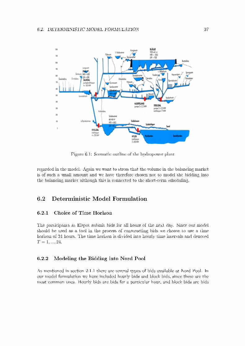
6.2. DETERMINISTIC MODEL FORMULATION 37
Figure 6.1: Scematic outline of the hydropower plant
regarded in the model. Again we want to stress that the volume in the balancing marketis of such a small amount and we have therefore chosen not to model the bidding intothe balancing market although this is connected to the short-term scheduling.
6.2 Deterministic Model Formulation
6.2.1 Choice of Time Horizon
The participants at Elspot submit bids for all hours of the next day. Since our modelshould be used as a tool in the process of constructing bids we choose to use a timehorizon of 24 hours. The time horizon is divided into hourly time intervals and denotedT = 1, ..., 24.
6.2.2 Modeling the Bidding into Nord Pool
As mentioned in section 2.1.1 there are several types of bids available at Nord Pool. Inour model formulation we have included hourly bids and block bids, since these are themost common ones. Hourly bids are bids for a particular hour, and block bids are bids
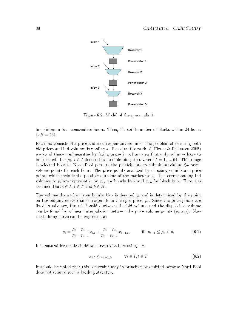
38 CHAPTER 6. CASE STUDY
Figure 6.2: Model of the power plant
for minimum four consecutive hours. Thus, the total number of blocks within 24 hoursis B = 231.
Each bid consists of a price and a corresponding volume. The problem of selecting bothbid prices and bid volumes is nonlinear. Based on the work of (Fleten & Pettersen 2005)we avoid these nonlinearities by xing prices in advance so that only volumes have tobe selected. Let pi, i ∈ I denote the possible bid prices where I = 1, ..., 64. This rangeis selected because Nord Pool permits the participants to submit maximum 64 price-volume points for each hour. The price points are xed by choosing equidistant pricepoints which include the possible outcome of the market price. The corresponding bidvolumes to pi are represented by xi,t for hourly bids and xi,b for block bids. Here it isassumed that i ∈ I, t ∈ T and b ∈ B.
The volume dispatched from hourly bids is denoted yt and is determined by the pointon the bidding curve that corresponds to the spot price, ρt. Since the price points arexed in advance, the relationship between the bid volume and the dispatched volumecan be found by a linear interpolation between the price-volume points (pi, xi,t). Nowthe bidding curve can be expressed as
yt =ρt − pi−1
pi − pi−1xi,t +
pi − ρt
pi − pi−1xi−1,t, if pi−1 ≤ ρt < pi (6.1)
It is natural for a sales bidding curve to be increasing, i.e.
xi,t ≤ xi+1,t, ∀i ∈ I, t ∈ T (6.2)
It should be noted that this constraint may in principle be omitted because Nord Pooldoes not require such a bidding structure.
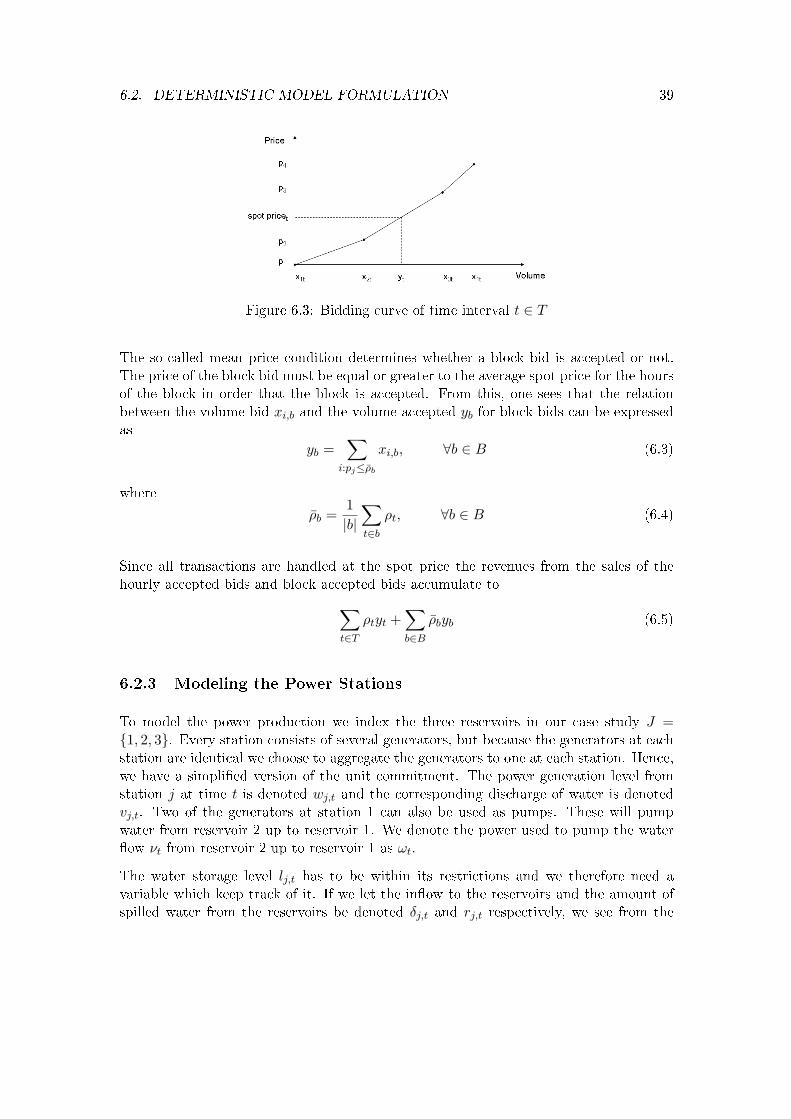
6.2. DETERMINISTIC MODEL FORMULATION 39
Figure 6.3: Bidding curve of time interval t ∈ T
The so-called mean price condition determines whether a block bid is accepted or not.The price of the block bid must be equal or greater to the average spot price for the hoursof the block in order that the block is accepted. From this, one sees that the relationbetween the volume bid xi,b and the volume accepted yb for block bids can be expressedas
yb =∑
i:pj≤ρb
xi,b, ∀b ∈ B (6.3)
where
ρb =1|b|∑t∈b
ρt, ∀b ∈ B (6.4)
Since all transactions are handled at the spot price the revenues from the sales of thehourly accepted bids and block accepted bids accumulate to∑
t∈T
ρtyt +∑b∈B
ρbyb (6.5)
6.2.3 Modeling the Power Stations
To model the power production we index the three reservoirs in our case study J =1, 2, 3. Every station consists of several generators, but because the generators at eachstation are identical we choose to aggregate the generators to one at each station. Hence,we have a simplied version of the unit commitment. The power generation level fromstation j at time t is denoted wj,t and the corresponding discharge of water is denotedvj,t. Two of the generators at station 1 can also be used as pumps. These will pumpwater from reservoir 2 up to reservoir 1. We denote the power used to pump the waterow νt from reservoir 2 up to reservoir 1 as ωt.
The water storage level lj,t has to be within its restrictions and we therefore need avariable which keep track of it. If we let the inow to the reservoirs and the amount ofspilled water from the reservoirs be denoted δj,t and rj,t respectively, we see from the
40 CHAPTER 6. CASE STUDY
discussion above that the water storage level at reservoir 1 at time t can be expressed as
l1,t = l1,t−1 − v1,t − r1,t + δ1,t + νt, ∀t ∈ T (6.6)
That is, the water storage level at time t is equal to the storage level at time t−1, minusthe water discharged and spilled and plus the natural inow and the water pumped upfrom reservoir 2.
Since the reservoirs are cascaded the water ow from an upper reservoir aects the waterstored in the underlying reservoirs. This must be allowed for in the expression for thewater storage level at reservoir 2 and 3. Since the reservoirs and stations are connectedthrough water gates were water always exists, we do not account for time delays betweenthe upper and lower reservoirs.
For reservoir 2 the water storage level at time t can be formulated as
l2,t = l2,t−1 − v2,t + v1,t − r2,t + δ2,t − νt, ∀t ∈ T (6.7)
Analogous for reservoir 3
l3,t = l3,t−1 − v3,t + v2,t − r3,t + δ3,t, ∀t ∈ T (6.8)
In addition, at time t = 0 the water storage level is given as lj,0.
All the variables must be within their borders. Thus,
lmin,j ≤ lj,t ≤ lmax,j , ∀j ∈ J, t ∈ T (6.9)
wmin,j ≤ wj,t ≤ wmax,j , ∀j ∈ J, t ∈ T (6.10)
vmin,j ≤ vj,t ≤ vmax,j , ∀j ∈ J, t ∈ T (6.11)
As mentioned in section 3.2.2, the power generated is a function of the water discharge andthe net water head of the power station. Whereas the headwater elevation is a function ofthe reservoir storage level, the tailwater elevation is a function of the discharge (Fleten &Kristoersen 2006). Because of our short time horizon we assume that the net water headdoes not vary much, and hence we assume that the power generated is only a functionof the water discharged from the reservoir.
The nonlinear relationship between the water ow, vj,t and the power generation may beapproximated by a concave function. Since we want to have a linear model we describethe concave fuction as a piecewise linear function with 4 linesegments. That is, wehave q = 1, ..., 5 discharge-generation points, (vj,q, wj,q) for every station. The pointsrepresent best-points of dierent sets of turbines at each station. These points were
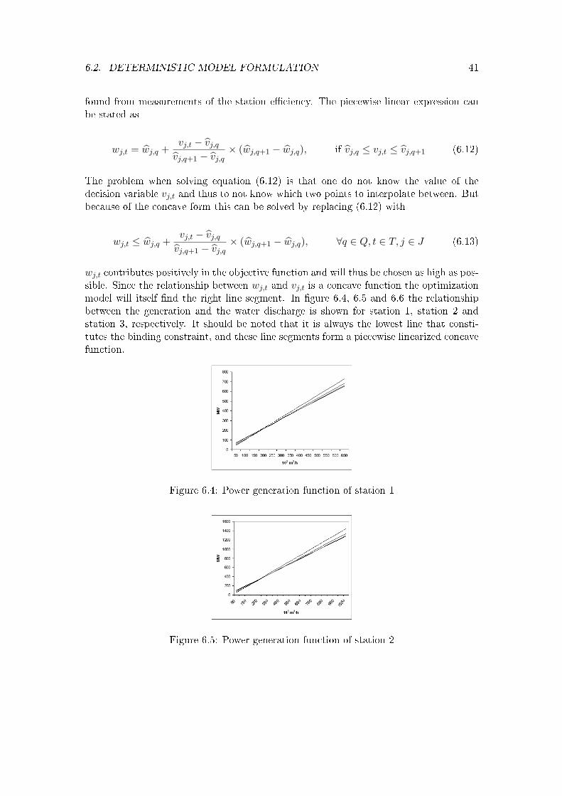
6.2. DETERMINISTIC MODEL FORMULATION 41
found from measurements of the station eciency. The piecewise linear expression canbe stated as
wj,t = wj,q +vj,t − vj,q
vj,q+1 − vj,q× (wj,q+1 − wj,q), if vj,q ≤ vj,t ≤ vj,q+1 (6.12)
The problem when solving equation (6.12) is that one do not know the value of thedecision variable vj,t and thus to not know which two points to interpolate between. Butbecause of the concave form this can be solved by replacing (6.12) with
wj,t ≤ wj,q +vj,t − vj,q
vj,q+1 − vj,q× (wj,q+1 − wj,q), ∀q ∈ Q, t ∈ T, j ∈ J (6.13)
wj,t contributes positively in the objective function and will thus be chosen as high as pos-sible. Since the relationship between wj,t and vj,t is a concave function the optimizationmodel will itself nd the right line segment. In gure 6.4, 6.5 and 6.6 the relationshipbetween the generation and the water discharge is shown for station 1, station 2 andstation 3, respectively. It should be noted that it is always the lowest line that consti-tutes the binding constraint, and these line segments form a piecewise linearized concavefunction.
Figure 6.4: Power generation function of station 1
Figure 6.5: Power generation function of station 2
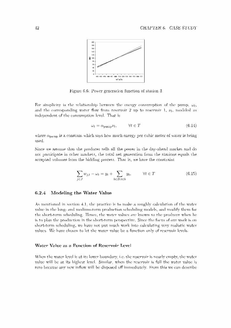
42 CHAPTER 6. CASE STUDY
Figure 6.6: Power generation function of station 3
For simplicity is the relationship between the energy consumption of the pump, ωt,and the corresponding water ow from reservoir 2 up to reservoir 1, νt, modeled asindependent of the consumption level. That is
ωt = αpumpνt, ∀t ∈ T (6.14)
where αpump is a constant which says how much energy per cubic meter of water is beingused.
Since we assume that the producer sells all the power in the day-ahead market and donot participate in other markets, the total net generation from the stations equals theaccepted volumes from the bidding process. That is, we have the constraint
∑j∈J
wj,t − ωt = yt +∑
b∈B:t∈b
yb, ∀t ∈ T (6.15)
6.2.4 Modeling the Water Value
As mentioned in section 4.1, the practice is to make a roughly calculation of the watervalue in the long- and medium-term production scheduling models, and modify them forthe short-term scheduling. Hence, the water values are known to the producer when heis to plan the production in the short-term perspective. Since the focus of our work is onshort-term scheduling, we have not put much work into calculating very realistic watervalues. We have chosen to let the water value be a function only of reservoir levels.
Water Value as a Function of Reservoir Level
When the water level is at its lower boundary, i.e. the reservoir is nearly empty, the watervalue will be at its highest level. Similar, when the reservoir is full the water value iszero because any new inow will be disposed o immediately. From this we can describe
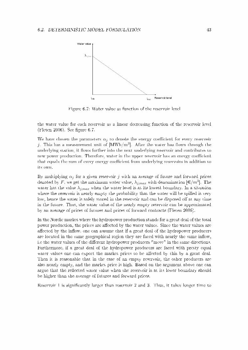
6.2. DETERMINISTIC MODEL FORMULATION 43
Figure 6.7: Water value as function of the reservoir level
the water value for each reservoir as a linear decreasing function of the reservoir level(Fleten 2006). See gure 6.7.
We have chosen the parameters αj to denote the energy coecient for every reservoirj. This has a measurement unit of [MWh/m3]. After the water has own through theunderlying station, it ows further into the next underlying reservoir and contributes tonew power production. Therefore, water in the upper reservoir has an energy coecientthat equals the sum of every energy coecient from underlying reservoirs in addition toits own.
By multiplying αj for a given reservoir j with an average of future and forward pricesdenoted by F , we get the maximum water value, λj,max with denomination [e/m3]. Thewater has the value λj,max when the water level is at its lowest boundary. In a situationwhere the reservoir is nearly empty the probability that the water will be spilled is verylow, hence the water is safely stored in the reservoir and can be disposed o at any timein the future. Thus, the water value of the nearly empty reservoir can be approximatedby an average of prices of futures and prices of forward contracts (Fleten 2006).
In the Nordic market where the hydropower production stands for a great deal of the totalpower production, the prices are aected by the water values. Since the water values areaected by the inow, one can assume that if a great deal of the hydropower producersare located in the same geographical region they are faced with nearly the same inow,i.e the water values of the dierent hydropower producers "move" in the same directions.Furthermore, if a great deal of the hydropower producers are faced with pretty equalwater values one can expect the market prices to be aected by this by a great deal.Then it is reasonable that in the case of an empty reservoir, the other producers arealso nearly empty, and the market price is high. Based on the argument above one canargue that the reected water value when the reservoir is at its lower boundary shouldbe higher than the average of futures and forward prices.
Reservoir 1 is signicantly larger than reservoir 2 and 3. Thus, it takes longer time to
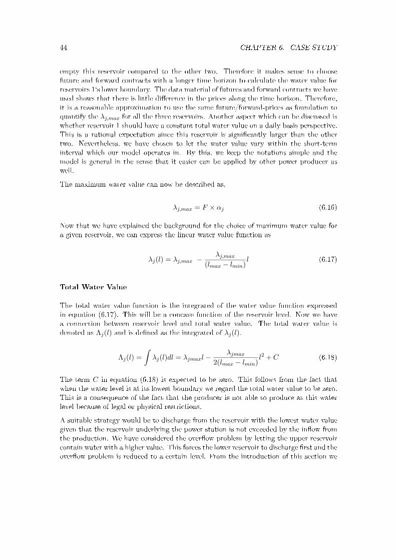
44 CHAPTER 6. CASE STUDY
empty this reservoir compared to the other two. Therefore it makes sense to choosefuture and forward contracts with a longer time horizon to calculate the water value forreservoirs 1`s lower boundary. The data material of futures and forward contracts we haveused shows that there is little dierence in the prices along the time horizon. Therefore,it is a reasonable approximation to use the same future/forward-prices as foundation toquantify the λj,max for all the three reservoirs. Another aspect which can be discussed iswhether reservoir 1 should have a constant total water value on a daily basis perspective.This is a rational expectation since this reservoir is signicantly larger than the othertwo. Nevertheless, we have chosen to let the water value vary within the short-terminterval which our model operates in. By this, we keep the notations simple and themodel is general in the sense that it easier can be applied by other power producer aswell.
The maximum water value can now be described as,
λj,max = F × αj (6.16)
Now that we have explained the background for the choice of maximum water value fora given reservoir, we can express the linear water value function as
λj(l) = λj,max − λj,max
(lmax − lmin)l (6.17)
Total Water Value
The total water value function is the integrated of the water value function expressedin equation (6.17). This will be a concave function of the reservoir level. Now we havea connection between reservoir level and total water value. The total water value isdenoted as Λj(l) and is dened as the integrated of λj(l).
Λj(l) =∫
λj(l)dl = λjmaxl − λjmax
2(lmax − lmin)l2 + C (6.18)
The term C in equation (6.18) is expected to be zero. This follows from the fact thatwhen the water level is at its lowest boundary we regard the total water value to be zero.This is a consequence of the fact that the producer is not able to produce at this waterlevel because of legal or physical restrictions.
A suitable strategy would be to discharge from the reservoir with the lowest water valuegiven that the reservoir underlying the power station is not exceeded by the inow fromthe production. We have considered the overow problem by letting the upper reservoircontain water with a higher value. This forces the lower reservoir to discharge rst and theoverow problem is reduced to a certain level. From the introduction of this section we
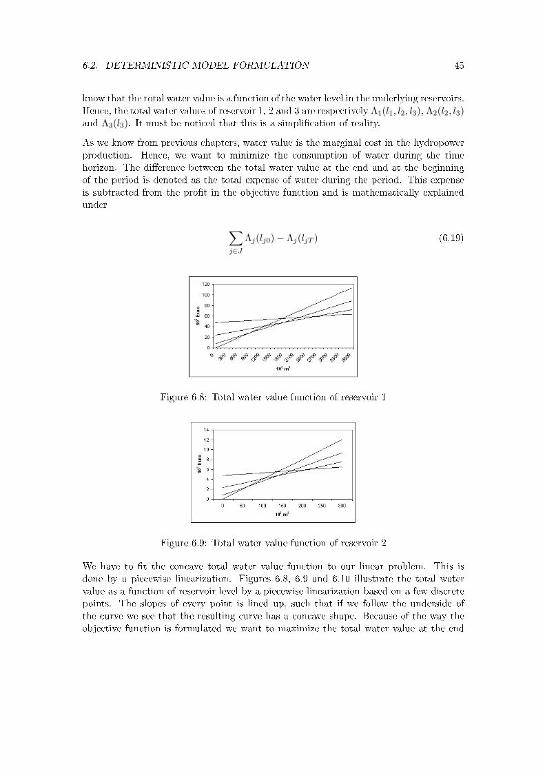
6.2. DETERMINISTIC MODEL FORMULATION 45
know that the total water value is a function of the water level in the underlying reservoirs.Hence, the total water values of reservoir 1, 2 and 3 are respectively Λ1(l1, l2, l3), Λ2(l2, l3)and Λ3(l3). It must be noticed that this is a simplication of reality.
As we know from previous chapters, water value is the marginal cost in the hydropowerproduction. Hence, we want to minimize the consumption of water during the timehorizon. The dierence between the total water value at the end and at the beginningof the period is denoted as the total expense of water during the period. This expenseis subtracted from the prot in the objective function and is mathematically explainedunder
∑j∈J
Λj(lj0)− Λj(ljT ) (6.19)
Figure 6.8: Total water value function of reservoir 1
Figure 6.9: Total water value function of reservoir 2
We have to t the concave total water value function to our linear problem. This isdone by a piecewise linearization. Figures 6.8, 6.9 and 6.10 illustrate the total watervalue as a function of reservoir level by a piecewise linearization based on a few discretepoints. The slopes of every point is lined up, such that if we follow the underside ofthe curve we see that the resulting curve has a concave shape. Because of the way theobjective function is formulated we want to maximize the total water value at the end
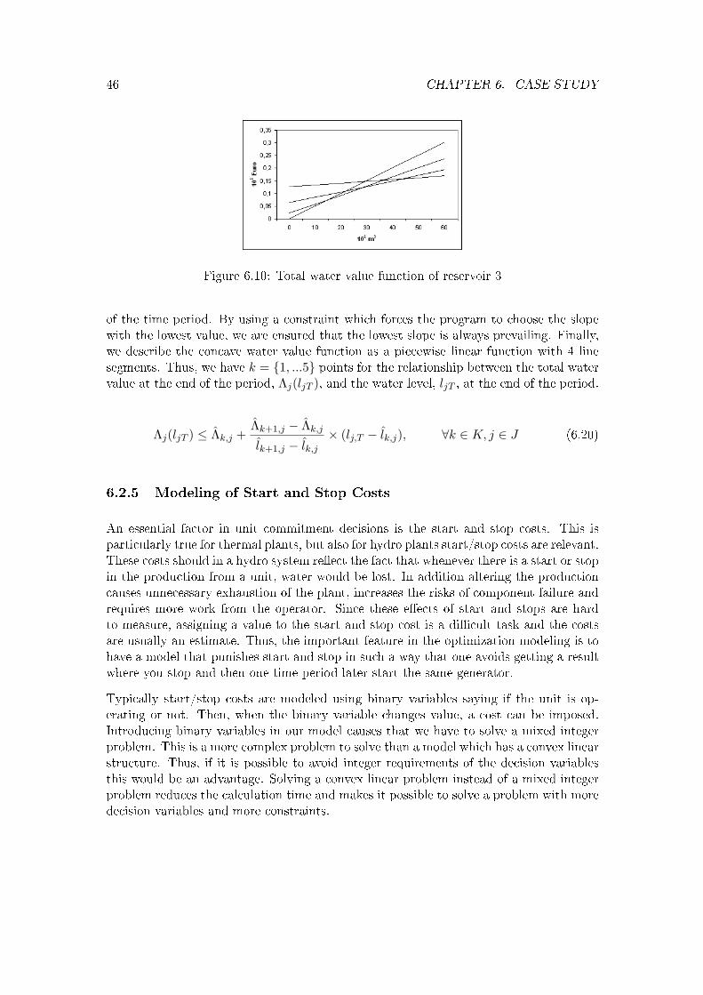
46 CHAPTER 6. CASE STUDY
Figure 6.10: Total water value function of reservoir 3
of the time period. By using a constraint which forces the program to choose the slopewith the lowest value, we are ensured that the lowest slope is always prevailing. Finally,we describe the concave water value function as a piecewise linear function with 4 linesegments. Thus, we have k = 1, ...5 points for the relationship between the total watervalue at the end of the period, Λj(ljT ), and the water level, ljT , at the end of the period.
Λj(ljT ) ≤ Λk,j +Λk+1,j − Λk,j
lk+1,j − lk,j
× (lj,T − lk,j), ∀k ∈ K, j ∈ J (6.20)
6.2.5 Modeling of Start and Stop Costs
An essential factor in unit commitment decisions is the start and stop costs. This isparticularly true for thermal plants, but also for hydro plants start/stop costs are relevant.These costs should in a hydro system reect the fact that whenever there is a start or stopin the production from a unit, water would be lost. In addition altering the productioncauses unnecessary exhaustion of the plant, increases the risks of component failure andrequires more work from the operator. Since these eects of start and stops are hardto measure, assigning a value to the start and stop cost is a dicult task and the costsare usually an estimate. Thus, the important feature in the optimization modeling is tohave a model that punishes start and stop in such a way that one avoids getting a resultwhere you stop and then one time period later start the same generator.
Typically start/stop costs are modeled using binary variables saying if the unit is op-erating or not. Then, when the binary variable changes value, a cost can be imposed.Introducing binary variables in our model causes that we have to solve a mixed integerproblem. This is a more complex problem to solve than a model which has a convex linearstructure. Thus, if it is possible to avoid integer requirements of the decision variablesthis would be an advantage. Solving a convex linear problem instead of a mixed integerproblem reduces the calculation time and makes it possible to solve a problem with moredecision variables and more constraints.

6.2. DETERMINISTIC MODEL FORMULATION 47
In our model we use the approximated formulation used by Weber in (Weber 2004) todescribe start and stop costs. When using this approximation one avoids binary decisionvariables by dening an additional decision variable, wonline
j,t which represents the capacity
currently online at station j at time step t. Within this model, wonlinej,t forms an articial
upper bound to the power output and multiplied with the quotient of maximum andminimum output it also forms a lower bound to the power output.
wj,t ≤ wonlinej,t ≤ wmax, ∀j ∈ J, t ∈ T (6.21)
(wmin
wmax
)× wonline
j,t ≤ wj,t, ∀j ∈ J, t ∈ T (6.22)
If the capacity online is increasing over time, that is if wonlinej,t > wonline
j,t−1 , start-up costsarise. Thus, the start-up cost function can be dened in the following way:
Cstart(wonline
j,t , wonlinej,t−1
)=
cstartj (wj,t − wj,t−1) if wonline
j,t > wonlinej,t−1
0 else(6.23)
On the other and if the capacity online is decreasing over time, i.e. wonlinej,t < wonline
j,t−1 ,stop costs arise.
Cstop(wonline
j,t , wonlinej,t−1
)=
cstopj (wj,t−1 − wj,t) if wonline
j,t < wonlinej,t−1
0 else(6.24)
Since wonlinej,t and wonline
j,t−1 both are decision variables, equation (6.23) and (6.24) aredicult to solve. To cope with this problem we have instead of equation (6.23) and(6.24) used the following equations which states the same
Cstartj,t ≥ cstart
j (wj,t − wj,t−1) , ∀j ∈ J, t ∈ T (6.25)
Cstartj,t ≥ 0, ∀j ∈ J, t ∈ T (6.26)
Cstopj,t ≥ cstop
j (wj,t−1 − wj,t) , ∀j ∈ J, t ∈ T (6.27)
Cstopj,t ≥ 0, ∀j ∈ J, t ∈ T (6.28)
The start and stop function contributes negatively in the object function. MinimizingCstart
j,t and Cstopj,t requires that the capacity online should be stable for each unit over
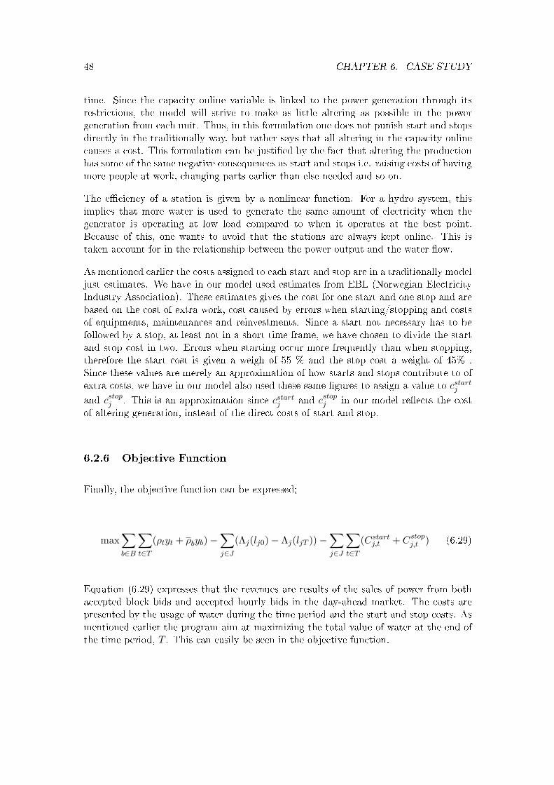
48 CHAPTER 6. CASE STUDY
time. Since the capacity online variable is linked to the power generation through itsrestrictions, the model will strive to make as little altering as possible in the powergeneration from each unit. Thus, in this formulation one does not punish start and stopsdirectly in the traditionally way, but rather says that all altering in the capacity onlinecauses a cost. This formulation can be justied by the fact that altering the productionhas some of the same negative consequences as start and stops i.e. raising costs of havingmore people at work, changing parts earlier than else needed and so on.
The eciency of a station is given by a nonlinear function. For a hydro system, thisimplies that more water is used to generate the same amount of electricity when thegenerator is operating at low load compared to when it operates at the best point.Because of this, one wants to avoid that the stations are always kept online. This istaken account for in the relationship between the power output and the water ow.
As mentioned earlier the costs assigned to each start and stop are in a traditionally modeljust estimates. We have in our model used estimates from EBL (Norwegian ElectricityIndustry Association). These estimates gives the cost for one start and one stop and arebased on the cost of extra work, cost caused by errors when starting/stopping and costsof equipments, maintenances and reinvestments. Since a start not necessary has to befollowed by a stop, at least not in a short time frame, we have chosen to divide the startand stop cost in two. Errors when starting occur more frequently than when stopping,therefore the start cost is given a weigh of 55 % and the stop cost a weight of 45% .Since these values are merely an approximation of how starts and stops contribute to ofextra costs, we have in our model also used these same gures to assign a value to cstart
j
and cstopj . This is an approximation since cstart
j and cstopj in our model reects the cost
of altering generation, instead of the direct costs of start and stop.
6.2.6 Objective Function
Finally, the objective function can be expressed;
max∑b∈B
∑t∈T
(ρtyt + ρbyb)−∑j∈J
(Λj(lj0)− Λj(ljT ))−∑j∈J
∑t∈T
(Cstartj,t + Cstop
j,t ) (6.29)
Equation (6.29) expresses that the revenues are results of the sales of power from bothaccepted block bids and accepted hourly bids in the day-ahead market. The costs arepresented by the usage of water during the time period and the start and stop costs. Asmentioned earlier the program aim at maximizing the total value of water at the end ofthe time period, T . This can easily be seen in the objective function.
6.3. THE STOCHASTIC PROGRAMMING MODEL 49
6.3 The Stochastic Programming Model
The model described in the last section does not reect the fact that both day-aheadprices and water inow are uncertain. To regard the uncertainty we apply a discreteprobability distribution of the uncertain data of price and inow. One way to approx-imate the continuous distributions into a discrete distribution is to use a scenario treeas described in section 5.3.1. The total number of scenarios is denoted by S. Further-more, each scenario is denoted by s with a corresponding probability πs. Finally, we canintroduce the two-stage stochastic programming model as a deterministic equivalent
max∑s∈S
πs
∑t∈T
∑b∈B
(ρt,syt,s + ρb,syb,s)−∑j∈J
(Λj(lj0,s)− Λj(ljT,s))−∑j∈J
∑t∈T
(Cstartj,t,s + Cstop
j,t,s )
(6.30)
subject to
Λj,s,T (lj) ≤ Λk,j +Λk+1,j − Λk,j
lk+1,j − lk,j
× (lj,s,T − lk,j), ∀j ∈ J, k ∈ K, s ∈ S (6.31)
yt,s =ρt,s − pi−1
pi − pi−1xi,t +
pi − ρt
pi − pi−1xi−1,t, ∀i ∈ I, t ∈ T, s ∈ S (6.32)
wj,t,s ≤ wj,q +vj,t,s − vj,q
vj,q+1 − vj,q× (wj,q+1 − wj,q), ∀q ∈ Q, t ∈ T, j ∈ J, s ∈ S (6.33)
Cstartj,t,s ≥ cstart
j (wj,t,s − wj,t−1,s) , ∀j ∈ J, t ∈ T, s ∈ S (6.34)
Cstopj,t,s ≥ cstop
j (wj,t−1,s − wj,t,s) , ∀j ∈ J, t ∈ T, s ∈ S (6.35)
∑j∈J
wj,t,s − ωt,s = yt,s +∑
b∈B:t∈b
yb,s, ∀t ∈ T, s ∈ S (6.36)
l1,t,s = l1,t−1 − v1,t,s − r1,t,s + δ1,t,s + νt,s, ∀t ∈ T, s ∈ S (6.37)
l2,t,s = l2,t−1 − v2,t,s + v1,t,s − r2,t,s + δ2,t,s − νt,s, ∀t ∈ T, s ∈ S (6.38)
50 CHAPTER 6. CASE STUDY
l3,t,s = l3,t−1 − v3,t,s + v2,t,s − r3,t,s + δ3,t,s, ∀t ∈ T, s ∈ S (6.39)
xi,t ≤ xi+1,t, ∀i ∈ I, t ∈ T (6.40)
ωt = αpumpνt, ∀t ∈ T (6.41)
lmin,j ≤ lj,t,s ≤ lmax,j , ∀j ∈ J, t ∈ T, s ∈ S (6.42)
wmin,j ≤ wj,t,s ≤ wmax,j , ∀j ∈ J, t ∈ T, s ∈ S (6.43)
vmin,j ≤ vj,t,s ≤ vmax,j , ∀j ∈ J, t ∈ T, s ∈ S (6.44)
wj,t,s ≤ wonlinej,t,s ≤ wmax, ∀j ∈ J, t ∈ T, s ∈ S (6.45)
(wmin
wmax
)× wonline
j,t,s ≤ wj,t,s, ∀j ∈ J, t ∈ T, s ∈ S (6.46)
Cstartj,t,s ≥ 0, ∀j ∈ J, t ∈ T, s ∈ S (6.47)
Cstopj,t,s ≥ 0, ∀j ∈ J, t ∈ T, s ∈ S (6.48)
6.4 Scenario Generation
6.4.1 Application of the HKW Algorithm
We choose to use the HKW algorithm for scenario generation. For further informationabout the HKW algorithm see section 5.4.2 or (Høyland et al. 2003). In our optimizationmodel of the bidding process the day-ahead market price and the inow to the twolower situated reservoirs are stochastic variables. Inow to reservoir 1 is anticipated tobe deterministic because of reservoir 1s magnitude. Since we want to construct a priceprole for every scenario, we generate scenarios for price and for price standard deviation.In addition we generate scenarios for the inow to reservoir 2 and 3.
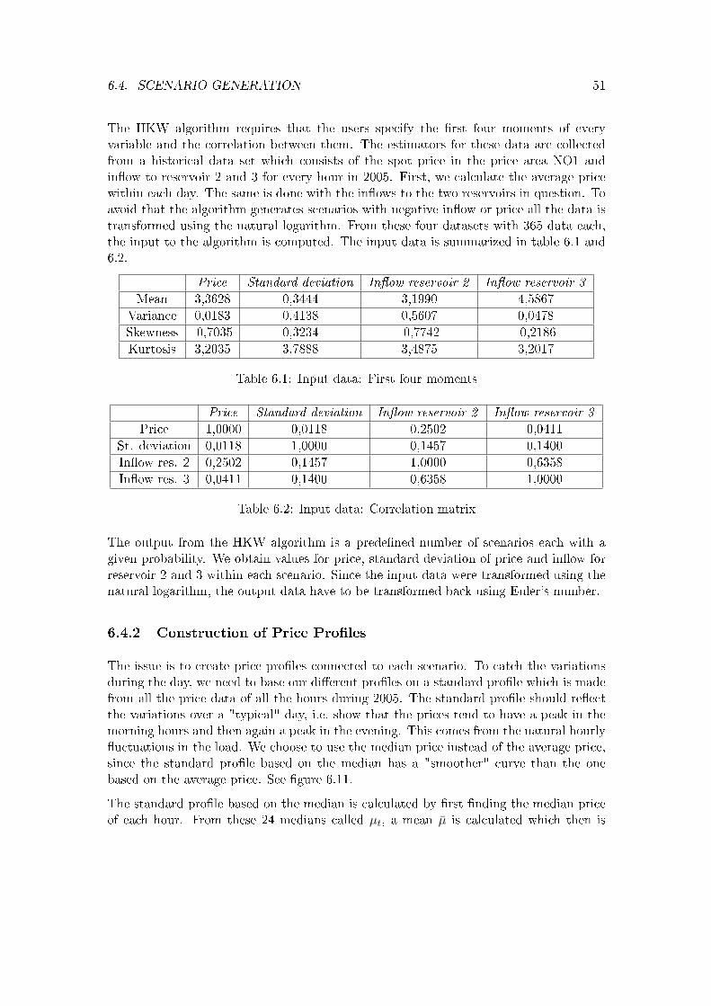
6.4. SCENARIO GENERATION 51
The HKW algorithm requires that the users specify the rst four moments of everyvariable and the correlation between them. The estimators for these data are collectedfrom a historical data set which consists of the spot price in the price area NO1 andinow to reservoir 2 and 3 for every hour in 2005. First, we calculate the average pricewithin each day. The same is done with the inows to the two reservoirs in question. Toavoid that the algorithm generates scenarios with negative inow or price all the data istransformed using the natural logarithm. From these four datasets with 365 data each,the input to the algorithm is computed. The input data is summarized in table 6.1 and6.2.
Price Standard deviation Inow reservoir 2 Inow reservoir 3
Mean 3,3628 0,3444 3,1990 4,5867
Variance 0,0183 0,4138 0,5607 0,0478
Skewness -0,7035 0,3234 -0,7742 -0,2186
Kurtosis 3,2035 3,7888 3,4875 3,2017
Table 6.1: Input data: First four moments
Price Standard deviation Inow reservoir 2 Inow reservoir 3
Price 1,0000 0,0118 0,2502 0,0411
St. deviation 0,0118 1,0000 0,1457 0,1400
Inow res. 2 0,2502 0,1457 1,0000 0,6358
Inow res. 3 0,0411 0,1400 0,6358 1,0000
Table 6.2: Input data: Correlation matrix
The output from the HKW algorithm is a predened number of scenarios each with agiven probability. We obtain values for price, standard deviation of price and inow forreservoir 2 and 3 within each scenario. Since the input data were transformed using thenatural logarithm, the output data have to be transformed back using Euler's number.
6.4.2 Construction of Price Proles
The issue is to create price proles connected to each scenario. To catch the variationsduring the day, we need to base our dierent proles on a standard prole which is madefrom all the price data of all the hours during 2005. The standard prole should reectthe variations over a "typical" day, i.e. show that the prices tend to have a peak in themorning hours and then again a peak in the evening. This comes from the natural hourlyuctuations in the load. We choose to use the median price instead of the average price,since the standard prole based on the median has a "smoother" curve than the onebased on the average price. See gure 6.11.
The standard prole based on the median is calculated by rst nding the median priceof each hour. From these 24 medians called µt, a mean µ is calculated which then is
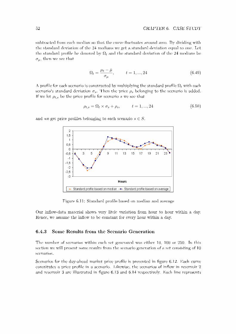
52 CHAPTER 6. CASE STUDY
subtracted from each median so that the curve uctuates around zero. By dividing withthe standard deviation of the 24 medians we get a standard deviation equal to one. Letthe standard prole be denoted by Ωt and the standard deviation of the 24 medians beσµ, then we see that
Ωt =µt − µ
σµ, t = 1, ..., 24 (6.49)
A prole for each scenario is constructed by multiplying the standard prole Ωt with eachscenario`s standard deviation σs. Then the price ρs belonging to the scenario is added.If we let ρt,s be the price prole for scenario s we see that
ρt,s = Ωt × σs + ρs, t = 1, ..., 24 (6.50)
and we get price proles belonging to each scenario s ∈ S.
Figure 6.11: Standard prole based on median and average
Our inow-data material shows very little variation from hour to hour within a day.Hence, we assume the inow to be constant for every hour within a day.
6.4.3 Some Results from the Scenario Generation
The number of scenarios within each set generated was either 10, 100 or 250. In thissection we will present some results from the scenario generation of a set consisting of 10scenarios.
Scenarios for the day-ahead market price prole is presented in gure 6.12. Each curveconstitutes a price prole in a scenario. Likewise, the scenarios of inow in reservoir 2and reservoir 3 are illustrated in gure 6.13 and 6.14 respectively. Each line represents
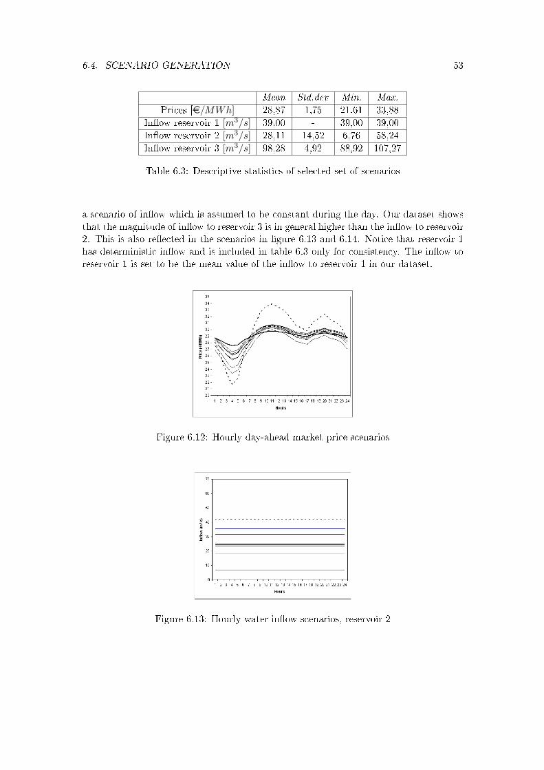
6.4. SCENARIO GENERATION 53
Mean Std.dev Min. Max.
Prices [e/MWh] 28,87 1,75 21,61 33,88
Inow reservoir 1 [m3/s] 39,00 - 39,00 39,00
Inow reservoir 2 [m3/s] 28,11 14,52 6,76 58,24
Inow reservoir 3 [m3/s] 98,28 4,92 88,92 107,27
Table 6.3: Descriptive statistics of selected set of scenarios
a scenario of inow which is assumed to be constant during the day. Our dataset showsthat the magnitude of inow to reservoir 3 is in general higher than the inow to reservoir2. This is also reected in the scenarios in gure 6.13 and 6.14. Notice that reservoir 1has deterministic inow and is included in table 6.3 only for consistency. The inow toreservoir 1 is set to be the mean value of the inow to reservoir 1 in our dataset.
Figure 6.12: Hourly day-ahead market price scenarios
Figure 6.13: Hourly water inow scenarios, reservoir 2
54 CHAPTER 6. CASE STUDY
Figure 6.14: Hourly water inow scenarios, reservoir 3
6.5 Computational Results
We have applied both the deterministic and the stochastic programming model to thecase. The deterministic model runs with the average of the ve sets of the 10-scenarios,while the stochastic model is tested for 10, 100 and 250 scenarios respectively. Theoptimization tool applied is Xpress Version 1.6.2. on a Pentium 4 2.4 GHz processor with256 MB RAM.
6.5.1 Initial Conditions
We have chosen to let the initial conditions for the reservoir levels be 50% of maximumlevel. The initial value of wonline
j,t=0 is set to maximum production for each reservoir. Seeappendix A for more information on input data in the model.
6.5.2 General Results
Table 6.4 sum up the computational results when we have applied dierent numbers ofscenarios. An interesting information from the table is that the objective value from thedeterministic solution (1 scenario) is consequently lower than the objective values in thestochastic solutions. This can also be conrmed by taking a glance at tables 6.5, 6.6,6.7 and 6.8. This might indicate that the stochastic model performs better than thedeterministic model in general. In addition, the objective value increases with increasingnumber of scenarios. A reason for this might be that the discrete distribution of thestochastic parameters becomes a better approximation of the real continuous distributionwith more scenarios. The computational solution time increases with increasing scenarios.This is an unavoidable disadvantage when the number of scenarios and hence the numberof variables increases.

6.5. COMPUTATIONAL RESULTS 55
Scenario Variables Constraints Objective value [e] Solution time [sec]
1 10538 2548 572301 0,02
10 18688 11872 572404 2,6
100 91915 105112 572386 86
250 215102 260512 572560 741,52
Table 6.4: Computational results
In section 6.5.3 one sees that it is optimal to produce at maximum capacity in bothscenarios in almost all hours. It should be noted that the model nd it optimal toproduce at maximum capacity for almost all hours in most of the scenarios, independentof which set of scenarios applied. This might indicate that the water values are set toolow or that the costs of altering production, i.e. the approximated start and stop costsare set too high.
6.5.3 Results from a Selected Set of Scenarios
We have chosen a set of 10 scenarios to illustrate some more results. If the reader lookback at gure 6.12, the bold line represents scenario 1 and is the scenario with the lowestvariance. The dotted line represents scenario 4 which has the greatest variance. Figure6.15 and 6.16 illustrate how the optimal production progresses during a day when themarket price does not uctuate remarkably, i.e. scenario 1 is prevailing, and when it isvolatile as in scenario 4.
Figure 6.15: Accepted volume, scenario 1
Figure 6.15 states that in scenario 1 the optimal action is to produce at maximumcapacity for all the hours during the day. We nd this reasonable because the spot priceis held steady higher than the water value for all the hours. In gure 6.16 one sees thatin scenario 4 one does not want to produce at maximum capacity for all the hours. Thisis also consistent with how the hourly prices uctuate as illustrated in gure 6.12. When

56 CHAPTER 6. CASE STUDY
Figure 6.16: Accepted volume, scenario 4
the price moves down as in hour 3, 4 and 5, it is obviously not optimal to produce atmaximum capacity.
Figure 6.17: Bid volume hour 3
To illustrate the shape of the bidding curve an example hour is chosen. Figure 6.17 showsthe optimal bid curve for hour 3 when the model is run with the 10 scenario set. The bidcurve is constructed by aggregating the hourly bids for hour 3 and the block bids whichapply hour 3. The gure shows that the model nds it optimal to bid approximately1900 MW at a price as low as zero. This high volume indicates that we probably haveset the water values too low. In the model we have not restricted the bid volume andas a consequence one sees that the total bid volume exceeds the maximum generationcapacity.
6.5.4 Stability Test
To test for stability ve sets of scenarios are made for respectively the 10, 100 and250 scenario-case. We have carried out the in-stability test described in section 5.3.2.
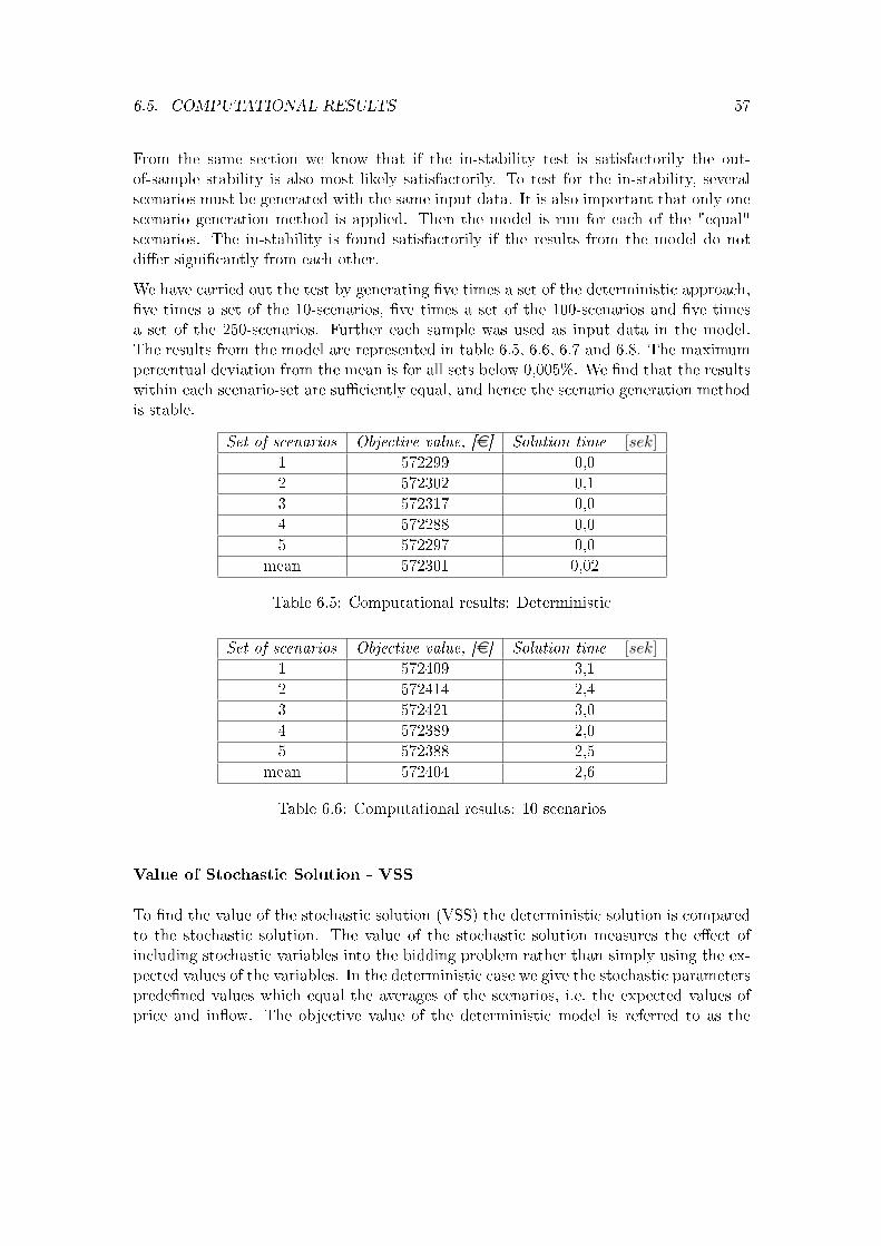
6.5. COMPUTATIONAL RESULTS 57
From the same section we know that if the in-stability test is satisfactorily the out-of-sample stability is also most likely satisfactorily. To test for the in-stability, severalscenarios must be generated with the same input data. It is also important that only onescenario generation method is applied. Then the model is run for each of the "equal"scenarios. The in-stability is found satisfactorily if the results from the model do notdier signicantly from each other.
We have carried out the test by generating ve times a set of the deterministic approach,ve times a set of the 10-scenarios, ve times a set of the 100-scenarios and ve timesa set of the 250-scenarios. Further each sample was used as input data in the model.The results from the model are represented in table 6.5, 6.6, 6.7 and 6.8. The maximumpercentual deviation from the mean is for all sets below 0,005%. We nd that the resultswithin each scenario-set are suciently equal, and hence the scenario generation methodis stable.
Set of scenarios Objective value, [e] Solution time [sek]1 572299 0,0
2 572302 0,1
3 572317 0,0
4 572288 0,0
5 572297 0,0
mean 572301 0,02
Table 6.5: Computational results: Deterministic
Set of scenarios Objective value, [e] Solution time [sek]1 572409 3,1
2 572414 2,4
3 572421 3,0
4 572389 2,0
5 572388 2,5
mean 572404 2,6
Table 6.6: Computational results: 10 scenarios
Value of Stochastic Solution - VSS
To nd the value of the stochastic solution (VSS) the deterministic solution is comparedto the stochastic solution. The value of the stochastic solution measures the eect ofincluding stochastic variables into the bidding problem rather than simply using the ex-pected values of the variables. In the deterministic case we give the stochastic parameterspredened values which equal the averages of the scenarios, i.e. the expected values ofprice and inow. The objective value of the deterministic model is referred to as the
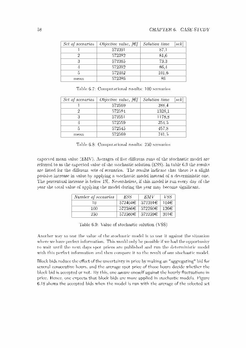
58 CHAPTER 6. CASE STUDY
Set of scenarios Objective value, [e] Solution time [sek]1 572391 87,1
2 572382 81,6
3 572365 73,3
4 572392 86,4
5 572402 101,6
mean 572386 86
Table 6.7: Computational results: 100 scenarios
Set of scenarios Objective value, [e] Solution time [sek]1 572560 388,4
2 572584 1328,1
3 572551 1178,8
4 572559 354,5
5 572545 457,8
mean 572560 741,5
Table 6.8: Computational results: 250 scenarios
expected mean value (EMV). Averages of ve dierent runs of the stochastic model arereferred to as the expected value of the stochastic solution (ESS). In table 6.9 the resultsare listed for the dierent sets of scenarios. The results indicate that there is a slightpositive increase in value by applying a stochastic model instead of a deterministic one.The percentual increase is below 1%. Nevertheless, if this model is run every day of theyear the total value of applying the model during the year may become signicant.
Number of scenarios ESS EMV VSS
10 572404e 572301e 104e100 572386e 572260e 126e250 572560e 572259e 301e
Table 6.9: Value of stochastic solution (VSS)
Another way to test the value of the stochastic model is to test it against the situationwhere we have perfect information. This would only be possible if we had the opportunityto wait until the next days spot prices are published and run the deterministic modelwith this perfect information and then compare it to the result of our stochastic model.
Block bids reduce the eect of the uncertainty in price by making an "aggregating" bid forseveral consecutive hours, and the average spot price of those hours decide whether theblock bid is accepted or not. By this, one assure oneself against the hourly uctuations inprice. Hence, one expects that block bids are more applied in stochastic models. Figure6.18 shows the accepted bids when the model is run with the average of the selected set
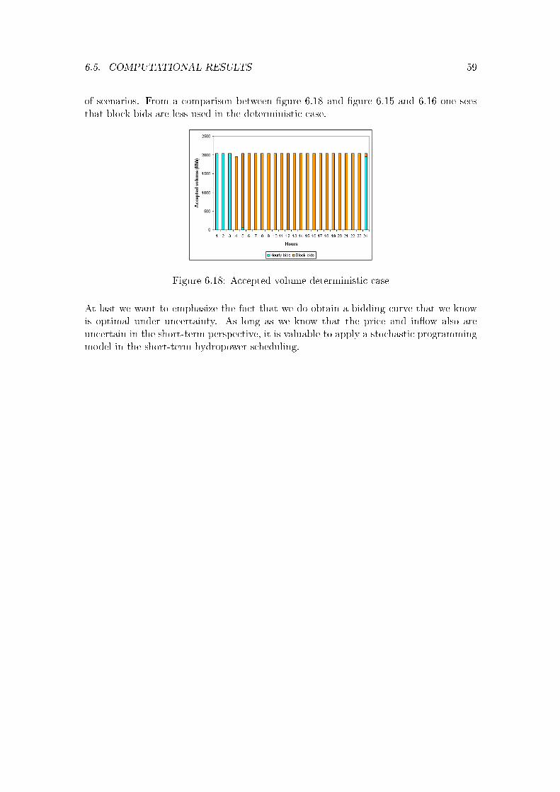
6.5. COMPUTATIONAL RESULTS 59
of scenarios. From a comparison between gure 6.18 and gure 6.15 and 6.16 one seesthat block bids are less used in the deterministic case.
Figure 6.18: Accepted volume deterministic case
At last we want to emphasize the fact that we do obtain a bidding curve that we knowis optimal under uncertainty. As long as we know that the price and inow also areuncertain in the short-term perspective, it is valuable to apply a stochastic programmingmodel in the short-term hydropower scheduling.
Chapter 7
Conclusion and Future Work
7.1 Conclusion
We have presented a short-term scheduling model for a hydropower station which regardthe uncertainty in the price and inow in the short-term perspective.
Our results show that there is a slight improvement in the objective value when thestochastic model is applied instead of the deterministic one. Even though, the percentualincrease is rather low one should keep in mind that the day-ahead bidding is done everyday. Hence, the accumulated increase in prot may become signicant over the year.Stochastic models are often criticized for being computational demanding. The stochasticmodel presented has a satisfactory solution time, even with 250 scenarios.
It should be noted that the results are preliminary and future work is required to validatethe results. We will in this section present some areas were future research could be done.
7.2 Improving the Scenarios
The scenario generation is an important part of making the stochastic model. The qualityof the stochastic model is linked to the quality of the scenarios. This follows from thefact that the scenarios provide information to the model of how the stochastic variablesvary. If the scenarios are of bad quality, then the stochastic model is necessarily of badquality too.
Therefore, part of the future work should consist of improving the construction of sce-narios. One should carry out more comprehensive testing for stability in the scenariosincluding testing for dierent scenario generation methods. A well known problem inmaking the inow scenarios is that the inow is autocorrelated in time. Hence, it ispreferable to account for this when choosing scenario generation method. An alternative
60
7.3. IMPROVING THE MODEL 61
way of scenario generation is to base the scenarios on predictions of price and inowinstead of historical data as in the HKW-algorithm. The producers often make theirown prognoses of price and inow which can be utilized in the scenario generation. Inaddition to the predictions one should also take into account extreme situations whichcan be weighted with lower probabilities than the other scenarios.
Our results show that the objective value increases with the number of scenarios. Fromthis it is obvious that it is interesting to generate larger sets of scenarios. In addition, theapproximation of the continuous "real world" stochastic distribution becomes better themore discrete points in the discrete distribution, i.e. the more scenarios included in theset. With an increasing number of scenarios it is also interesting to see if the objectivevalue nally converges toward a certain value. This indicates how many scenarios that isneeded in the set. Furthermore, constructing better standard proles by either makingthem more specic to a certain day/season or by letting more stochastic variables describethem is left to future work.
7.3 Improving the model
It is clearly an advantage if the model is programmed more generic. This would make iteasy to adjust the model to other hydropower plants. A higher detailing level will describethe physical system better. In our model formulation we do not consider the generationat unit level only at station level. Since we have chosen best-points combination of theturbines to construct the station generation curves, the model nds a too good solution.This would be avoided if one modeled each unit explicitly. In addition it would beinteresting to compare our linear model with a mixed integer model. The latter modelwould have binary variables representing if the units are in operation or not, hence usethe standard formulation of start and stop costs.
The modeling of the water values should be improved in further work. The most appro-priate would be to use water values from the long- and medium-term scheduling modelsas input in the short-term model. In addition, a longer time horizon can be chosen toinclude the coupling to medium-term models. In such a case it would probably be properto use a multi-stage stochastic model. The time horizon could also be extended by in-cluding the hours before the bidding, then one would take into account the fact that noshort-term scheduling plan is independent from day to day.
In our model we have xed the price points by choosing equidistant price points whichinclude the possible outcome of the market price. Another way this could have been doneis to have equiprobable price points. Hence, the probability of being dispatched on anyof the I − 1 line segments is the same.

62 CHAPTER 7. CONCLUSION AND FUTURE WORK
7.4 Validation of the Model
Comparing the model against the regular practice of short-term scheduling is left tofuture work. That is to run the model over a period and compare the objective valuesagainst the real prot earned from bidding in the spot market during the same period.It is only through such a validation that one can throughly reveal whether a stochasticmodel performs better than common deterministic practice. The EVPI-test could alsobe accomplished in this setting.
The model can also be run for special designed scenarios to test how the model behavesin "extreme" situations. By this one would get an anticipation if the model acts rational,since one in "extreme" situations intuitively knows how the model optimally would act.

Bibliography
Belsnes, M., Honve, I. & Fosso, O. (2005), `Bidding in the secondary reserve market froma hydropower perspective', Presented at the 15th PSCC, Liege.
Birge, J. (1997), Introduction to stochastic programming, Springer, New York.
Box, G. & Jenkins, G. (1976), Time Series Analysis: forecasting and control, Holden-Day.
Brooks, C. (2004), Introductory econometrics for nance, Cambridge University Press.
Flatabø, N., Fosso, O., Haugstad, A. & Mo, B. (2002), `Hydro scheduling in competi-tive electricity markets, an overview', Workshop on Hydro Scheduling in CompetiveElectricity Markets, SINTEF Energy Research.
Fleten, S.-E. (2006), `Oral information from Stein-Erik Fleten'.
Fleten, S.-E. & Kristoersen, T. K. (2006), `Short-term hydropower production planningby stochastic programming', Accepted for publication in Computers and OperationsResearch.
Fleten, S.-E. & Pettersen, E. (2005), `Constructing bidding curves for a price-taker re-tailer in the Norwegian electricity market', IEEE Transactions on power systems20, 701 708.
Fleten, S.-E., Wallace, S. & Ziemba, W. (2002), `Hedging electricity portfolios via stochas-tic programming', C. Greengard and A. Ruszczynski (eds), Decision Making UnderUncertainty: Energy and Power, vol. 128 of IMA Volumes on Mathematics and ItsApplications pp. 7193.
Fosso, O. & Gjengedal, T. (2006), `Analysemetoder og vannverdiberegninger', Lecturesin TET14 Driftsplanlegging, NTNU.
Fosso, O., Haugstad, A. & Mo, B. (2006), `Produksjonsplanlegging i vannkraftbasertesystemer', Lectures in TET14 Driftsplanlegging, NTNU.
George, J., Read, E. & Kerr, A. (1995), `Optimal scheduling of hydro stations: An integerprogramming model', Working Paper EMRG-WP-95-08, University of Canterbury,Christchurch, New Zealand.
63

64 BIBLIOGRAPHY
Hreinsson, E. (1988), `Optimal short term operation of a purely hydroelectric system',IEEE Transactions on Power Systems 3, 1072 1077.
Høyland, K., Kaut, M. & Wallace, S. (2003), `A heuristic for moment-matching scenariogeneration', Computational Optimization and Applications 24, 169 185.
Johnsen, T., Verma, S. & Wolfram, C. (1999), `Zonal pricing and demand-side bidding inthe norwegian electricity market',Working Paper PWP-063, University of CaliforniaEnergy Institute.
Kall, P. & Wallace, S. (1994), Stochastic Programming, John Wiley and Sons Ltd., Chich-ester.
Kaut, M. & Wallace, S. (2003), `Evaluation of scenario-generation methods for stochasticprogramming', SPEPS, Working Paper 14.
NordPool (2004), `The Nordic Power Market - Electricity Power Exchangeacross National Borders', www.nordpool.no/information/reports/Report-Nordic%20Market.pdf.
NordPool (2006), `Bidding in Nord Pool Spot's Elspot Market',www.nordpoolspot.com/Documents/Product%20Sheets/Bidding%20in%20Elspot.pdf.
NVE (2006), www.nve.no/modules/module_109/publisher_view_product.asp?iEntityId=9768.
Philpott, A., Craddock, M. & Waterer, H. (2000), `Hydro-electric unit commitmentsubject to uncertain demand', European Journal of Operational Research 125, 410 424.
Tjøtta, E. (2006), `Presentation held by Erik Tjøtta, Statkraft', 12.10 in the lectures ofTET 14 Driftsplanlegging, NTNU.
Wallace, S. (1999), `Decision making under uncertainty: The art of modeling', NorwegianUniversity of Science and Technology.
Wangensteen, I. (2005), `Kraftmarkeder', Lectures in TET4185 Kraftmarkeder, NTNU.
Weber, C. (2004), Uncertainty in the electric power industry - Methods and Models forDecision Support, Springer, New York.
Wen, F. & David, A. (2001), `Strategic bidding for electricity supply in a day-aheadenergy market', Electric Power Systems Research 59, 197 206.

Appendix A
Input Data - Case Study
Reservoir Initial reservoir level [m3] wonlinej,t=0 [MW ]
1 1761500000 640
2 138185000 1240
3 29150000 160
Table A.1: Input data: Initial conditions in the model
Res. min. capacity [MW] max. capacity [MW] start cost [e] stop cost [e] F [e]1 100 640 206,25 168,8 35
2 200 1240 309,4 253,0 35
3 55 160 151,25 123,8 35
Table A.2: Data input
For more input data to the model, see the enclosed CD-ROM.
65

Appendix B
CD-ROM
The contents in the enclosed CD-ROM is:
• Xpress codes
• Input data to Xpress
• Input data to HKW algorithm
• Output data from HKW algorithm, ve sets of 10 scenarios
• Output data from HKW algorithm, ve sets of 100 scenarios
• Output data from HKW algorithm, ve sets of 250 scenarios
• The standard prole
66

Appendix C
Xpress Programming Codes
67

model "stochastic short-term scheduling" uses "mmxprs", "mmodbc"; !gain access to the Xpress-Optimizer solver declarations S=10 !number of scenarios T=24 !number of hours B: integer !number of block I=64 !number of price-steps J=3 !number of reservoirs L=5 ! number of line-points P=6 !number of efficiency-points O=2 !efficieny-points range time_24 = 1..T scenario = 1..S reservoir = 1..J block_data =1..3 price =1..I line_points = 1..L v_points = 1..P factor=1..O end-declarations B:= sum(t in time_24)t-24-23-22 declarations block = 1..B blocks:array(block_data,block)of integer !1.row:start,2.row:stop,3.row: #hours a:integer q:integer prob: array(scenario)of real !probability of each scenario to occur price_steps: array(price)of real !price-steps spotprice_h: array(time_24,scenario)of real !hourly spotprice from the scenarios spotprice_b: array(block,scenario)of real !block-prices made from hourly spot prices alpha: array(reservoir)of real !energy coefficient start_cost: array(reservoir)of real stopp_cost: array (reservoir)of real vmin: array(reservoir)of real !minimum level of water flow into a station vmax: array(reservoir)of real !maximum level of water flow into a station wmin: array(reservoir)of real !minimum level of generation wmax: array(reservoir)of real !maximum level of generation lmin: array(reservoir)of real !minimum level of reservoir lmax: array(reservoir)of real !maximum level of reservoir l_start: array(reservoir)of real !initial level at reservoirs value_start: array(reservoir)of real !initial value of water online_initiell: array(reservoir)of real !initial value of online-variable v_point1: array(v_points,factor)of real !waterflow points station 1 v_point2: array(v_points,factor)of real! waterflow points station 2 v_point3:array(v_points,factor)of real !waterflow points station 3 inflow:array(reservoir,scenario)of real !inflow
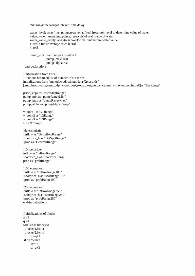
tau: array(reservoir)of integer !time delay water_level: array(line_points,reservoir)of real !reservoir level to determine value of water value_water: array(line_points, reservoir)of real !value of water water_value_empty: array(reservoir)of real !maximum water value F: real ! future average price [euro] k: real pump_min: real !pumps at station 1 pump_max: real pump_alpha:real end-declarations !Initialization from Excel !Here one has to adjust of number of scenarios initialisations from "mmodbc.odbc:input data Xpress.xls" [lmin,lmax,wmin,wmax,alpha,start_cost,stopp_cost,tau,l_start,vmin,vmax,online_initiell]as "ResRange" price_steps as "priceStepRange" pump_min as "pumpRangeMin" pump_max as "pumpRangeMax" pump_alpha as "pumpAlphaRange" v_point1 as "v1Range" v_point2 as "v2Range" v_point3 as "v3Range" F as "FRange" !deterministic !inflow as "DetInflowRange" !spotprice_h as "DetSpotRange" !prob as "DetProbRange" !10 scenarioer inflow as "inflowRange" spotprice_h as "spotPriceRange" prob as "probRange" !100 scenarioer !inflow as "inflowRange100" !spotprice_h as "spotRange100" !prob as "probRange100" !250 scenarioer !inflow as "inflowRange250" !spotprice_h as "spotRange250" !prob as "probRange250" end-initialisations !Initializations of blocks a:=1 q:=4 forall(b in block)do blocks(1,b):=a blocks(2,b):=q q:=q+1 if q=25 then a:=a+1 q:=a+3
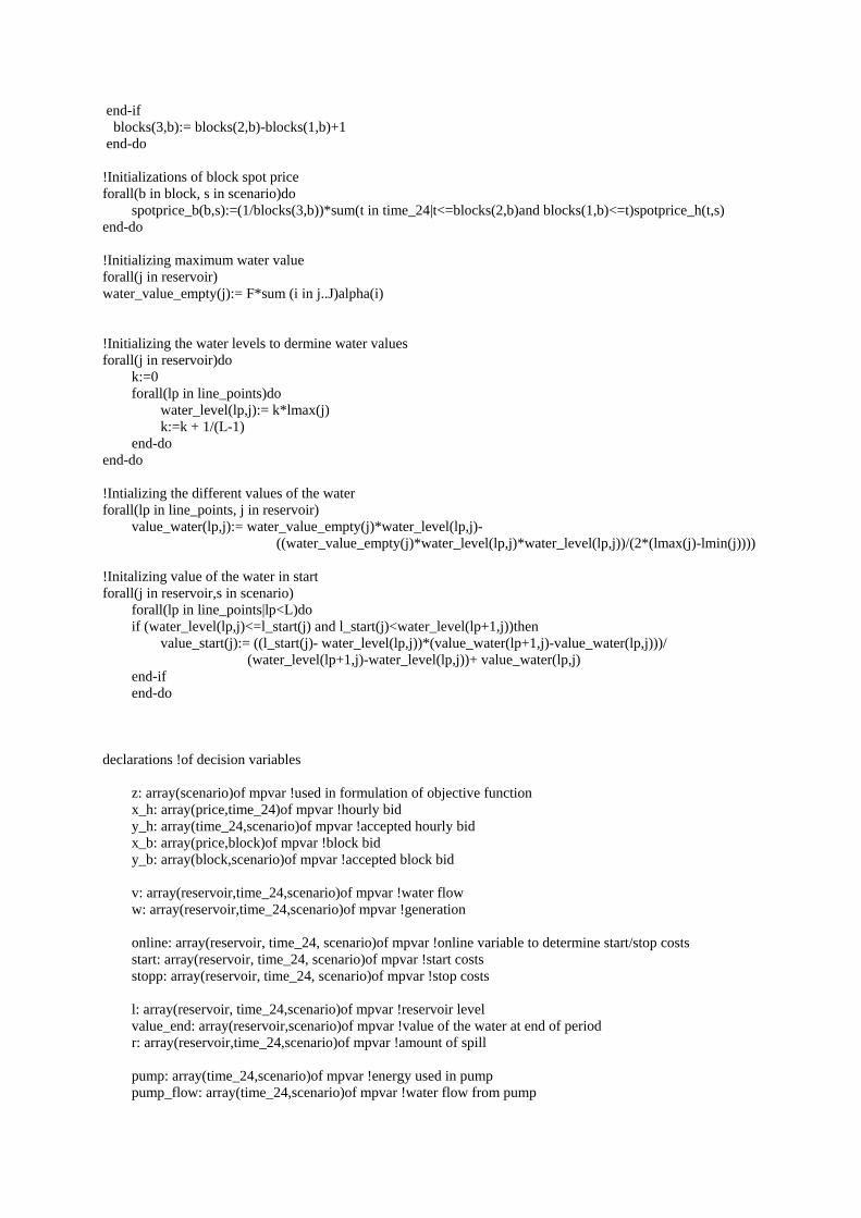
end-if blocks(3,b):= blocks(2,b)-blocks(1,b)+1 end-do !Initializations of block spot price forall(b in block, s in scenario)do spotprice_b(b,s):=(1/blocks(3,b))*sum(t in time_24|t<=blocks(2,b)and blocks(1,b)<=t)spotprice_h(t,s) end-do !Initializing maximum water value forall(j in reservoir) water_value_empty(j):= F*sum (i in j..J)alpha(i) !Initializing the water levels to dermine water values forall(j in reservoir)do k:=0 forall(lp in line_points)do water_level(lp,j):= k*lmax(j) k:=k + 1/(L-1) end-do end-do !Intializing the different values of the water forall(lp in line_points, j in reservoir) value_water(lp,j):= water_value_empty(j)*water_level(lp,j)- ((water_value_empty(j)*water_level(lp,j)*water_level(lp,j))/(2*(lmax(j)-lmin(j)))) !Initalizing value of the water in start forall(j in reservoir,s in scenario) forall(lp in line_points|lp<L)do if (water_level(lp,j)<=l_start(j) and l_start(j)<water_level(lp+1,j))then value_start(j):= ((l_start(j)- water_level(lp,j))*(value_water(lp+1,j)-value_water(lp,j)))/ (water_level(lp+1,j)-water_level(lp,j))+ value_water(lp,j) end-if end-do declarations !of decision variables z: array(scenario)of mpvar !used in formulation of objective function x_h: array(price,time_24)of mpvar !hourly bid y_h: array(time_24,scenario)of mpvar !accepted hourly bid x_b: array(price,block)of mpvar !block bid y_b: array(block,scenario)of mpvar !accepted block bid v: array(reservoir,time_24,scenario)of mpvar !water flow w: array(reservoir,time_24,scenario)of mpvar !generation online: array(reservoir, time_24, scenario)of mpvar !online variable to determine start/stop costs start: array(reservoir, time_24, scenario)of mpvar !start costs stopp: array(reservoir, time_24, scenario)of mpvar !stop costs l: array(reservoir, time_24,scenario)of mpvar !reservoir level value_end: array(reservoir,scenario)of mpvar !value of the water at end of period r: array(reservoir,time_24,scenario)of mpvar !amount of spill pump: array(time_24,scenario)of mpvar !energy used in pump pump_flow: array(time_24,scenario)of mpvar !water flow from pump

end-declarations !OBJECTIVE FUNCTION profit:= sum(s in scenario)(prob(s)*z(s)) !CONSTRAINTS forall(s in scenario) z(s)=((sum(t in time_24)spotprice_h(t,s)*y_h(t,s))+ !revenues hourly bids (sum(b in block)spotprice_b(b,s)*blocks(3,b)*y_b(b,s))+ !revenues block bids (sum(j in reservoir)value_end(j,s))- !total value of water at end (sum(j in reservoir)value_start(j))- ! total value of water at start (sum(j in reservoir,t in time_24)start(j,t,s))-!app. start costs (sum(j in reservoir,t in time_24)stopp(j,t,s)))!app. stop costs !the value of the water in the end if the end-level is between 1 and 2 forall(s in scenario,j in reservoir) value_end(j,s)<=((l(j,T,s)- water_level(1,j))*(value_water(2,j)-value_water(1,j)))/ (water_level(2,j)-water_level(1,j))+ value_water(1,j) !the value of the water in the end if the end-level is between 2 and 3 forall(s in scenario,j in reservoir) value_end(j,s)<=((l(j,T,s)- water_level(2,j))*(value_water(3,j)-value_water(2,j)))/ (water_level(3,j)-water_level(2,j))+ value_water(2,j) !the value of the water in the end if the end-level is between 3 and 4 forall(s in scenario,j in reservoir) value_end(j,s)<=((l(j,T,s)- water_level(3,j))*(value_water(4,j)-value_water(3,j)))/ (water_level(4,j)-water_level(3,j))+ value_water(3,j) !the value of the water in the end if the end-level is between 4 and 5 forall(s in scenario,j in reservoir) value_end(j,s)<=((l(j,T,s)- water_level(4,j))*(value_water(5,j)-value_water(4,j)))/ (water_level(5,j)-water_level(4,j))+ value_water(4,j) !Relationship between accepted volume and bid volume forall(t in time_24,s in scenario, i in 1..I-1| price_steps(i) <= spotprice_h(t,s) and price_steps(i+1) > spotprice_h(t,s))!) y_h(t,s)<=((spotprice_h(t,s)-price_steps(i))/(price_steps(i+1)-price_steps(i)))*x_h(i+1,t)+ ((price_steps(i+1)-spotprice_h(t,s))/(price_steps(i+1)-price_steps(i)))*x_h(i,t) forall(b in block, s in scenario) y_b(b,s)= sum(i in price|price_steps(i)<=spotprice_b(b,s))x_b(i,b) !Realation between generation and water flow at station 1 forall(j in reservoir,t in time_24,s in scenario|j=1) w(j,t,s)<=v_point1(1,1)+((v(j,t,s)-v_point1(1,2))/(v_point1(2,2)-v_point1(1,2)))*(v_point1(2,1)-v_point1(1,1)) forall(j in reservoir,t in time_24,s in scenario|j=1) w(j,t,s)<=v_point1(2,1)+((v(j,t,s)-v_point1(2,2))/(v_point1(3,2)-v_point1(2,2)))*(v_point1(3,1)-v_point1(2,1)) forall(j in reservoir,t in time_24,s in scenario|j=1) w(j,t,s)<=v_point1(3,1)+((v(j,t,s)-v_point1(3,2))/(v_point1(4,2)-v_point1(3,2)))*(v_point1(4,1)-v_point1(3,1)) forall(j in reservoir,t in time_24,s in scenario|j=1)

w(j,t,s)<=v_point1(4,1)+((v(j,t,s)-v_point1(4,2))/(v_point1(5,2)-v_point1(4,2)))*(v_point1(5,1)-v_point1(4,1)) forall(j in reservoir,t in time_24,s in scenario|j=1) w(j,t,s)<=v_point1(5,1)+((v(j,t,s)-v_point1(5,2))/(v_point1(6,2)-v_point1(5,2)))*(v_point1(6,1)-v_point1(5,1)) !Realation between generation and water flow at station 2 forall(j in reservoir,t in time_24,s in scenario|j=2) w(j,t,s)<=v_point2(1,1)+((v(j,t,s)-v_point2(1,2))/(v_point2(2,2)-v_point2(1,2)))*(v_point2(2,1)-v_point2(1,1)) forall(j in reservoir,t in time_24,s in scenario|j=2) w(j,t,s)<=v_point2(2,1)+((v(j,t,s)-v_point2(2,2))/(v_point2(3,2)-v_point2(2,2)))*(v_point2(3,1)-v_point2(2,1)) forall(j in reservoir,t in time_24,s in scenario|j=2) w(j,t,s)<=v_point2(3,1)+((v(j,t,s)-v_point2(3,2))/(v_point2(4,2)-v_point2(3,2)))*(v_point2(4,1)-v_point2(3,1)) forall(j in reservoir,t in time_24,s in scenario|j=2) w(j,t,s)<=v_point2(4,1)+((v(j,t,s)-v_point2(4,2))/(v_point2(5,2)-v_point2(4,2)))*(v_point2(5,1)-v_point2(4,1)) forall(j in reservoir,t in time_24,s in scenario|j=2) w(j,t,s)<=v_point2(5,1)+((v(j,t,s)-v_point2(5,2))/(v_point2(6,2)-v_point2(5,2)))*(v_point2(6,1)-v_point2(5,1)) !Realation between generation and water flow at station 3 forall(j in reservoir,t in time_24,s in scenario|j=3) w(j,t,s)<=v_point3(1,1)+((v(j,t,s)-v_point3(1,2))/(v_point3(2,2)-v_point3(1,2)))*(v_point3(2,1)-v_point3(1,1)) forall(j in reservoir,t in time_24,s in scenario|j=3) w(j,t,s)<=v_point3(2,1)+((v(j,t,s)-v_point3(2,2))/(v_point3(3,2)-v_point3(2,2)))*(v_point3(3,1)-v_point3(2,1)) forall(j in reservoir,t in time_24,s in scenario|j=3) w(j,t,s)<=v_point3(3,1)+((v(j,t,s)-v_point3(3,2))/(v_point3(4,2)-v_point3(3,2)))*(v_point3(4,1)-v_point3(3,1)) forall(j in reservoir,t in time_24,s in scenario|j=3) w(j,t,s)<=v_point3(4,1)+((v(j,t,s)-v_point3(4,2))/(v_point3(5,2)-v_point3(4,2)))*(v_point3(5,1)-v_point3(4,1)) forall(j in reservoir,t in time_24,s in scenario|j=3) w(j,t,s)<=v_point3(5,1)+((v(j,t,s)-v_point3(5,2))/(v_point3(6,2)-v_point3(5,2)))*(v_point3(6,1)-v_point3(5,1)) !Increacing bid curve forall(t in time_24,i in 1..(I-1)) x_h(i,t)<=x_h(i+1,t) !online constraints forall(j in reservoir, t in time_24, s in scenario) online(j,t,s)<=wmax(j) forall(j in reservoir, t in time_24, s in scenario) w(j,t,s)<=online(j,t,s) forall(j in reservoir, t in time_24, s in scenario) (wmin(j)/wmax(j))*online(j,t,s)<=w(j,t,s) !start/stop costs forall(j in reservoir, t in time_24, s in scenario) start(j,t,s)>=0
forall(j in reservoir, t in time_24, s in scenario|t=1) start(j,t,s)>=start_cost(j)*(online(j,t,s)-online_initiell(j)) forall(j in reservoir, t in time_24, s in scenario|t<T) start(j,t+1,s)>=start_cost(j)*(online(j,t+1,s)-online(j,t,s)) forall(j in reservoir, t in time_24, s in scenario) stopp(j,t,s)>=0 forall(j in reservoir, t in time_24, s in scenario|t=1) stopp(j,t,s)>=stopp_cost(j)*(online_initiell(j)-online(j,t,s)) forall(j in reservoir, t in time_24, s in scenario|t<T) stopp(j,t+1,s)>=stopp_cost(j)*(online(j,t,s)-online(j,t+1,s)) !generation equals accepted volume forall(t in time_24,s in scenario) sum(j in reservoir)w(j,t,s)-pump(t,s)=y_h(t,s)+ sum(b in block|t<=blocks(2,b)and blocks(1,b)<=t)y_b(b,s) !water flow within its restrictions forall(j in reservoir, t in time_24,s in scenario) vmin(j)<=v(j,t,s) forall(j in reservoir, t in time_24,s in scenario) v(j,t,s)>=vmax(j) !generation within its restrictions forall(j in reservoir, t in time_24, s in scenario) wmin(j)<=w(j,t,s) forall(j in reservoir, t in time_24, s in scenario) wmax(j)>=w(j,t,s) !reservoir within its restrictions forall(j in reservoir,t in time_24,s in scenario) lmin(j)<=l(j,t,s) forall(j in reservoir,t in time_24,s in scenario) lmax(j)>=l(j,t,s) !waterlevel balance at reservoir 1 forall(j in reservoir,t in time_24,s in scenario|j=1 and t=1) l(j,t,s)-l_start(j)+v(j,t,s)+r(j,t,s)=inflow(j,s)+ pump_flow(t,s) forall(j in reservoir, t in time_24,s in scenario|j=1 and t>1) l(j,t,s)-l(j,t-1,s)+v(j,t,s)+r(j,t,s)=inflow(j,s)+ pump_flow(t,s) !waterlevel balance at reservoir 2 forall(j in reservoir, t in time_24, s in scenario|j=2 and t=1 and t>tau(j)) l(j,t,s)-l_start(j)+v(j,t,s)+ r(j,t,s)=v(j-1,t-tau(j),s)+inflow(j,s)- pump_flow(t,s) forall(j in reservoir, t in time_24, s in scenario|j=2 and t>1 and t>tau(j)) l(j,t,s)-l(j,t-1,s)+v(j,t,s)+ r(j,t,s)=v(j-1,t-tau(j),s)+inflow(j,s)-pump_flow(t,s) forall(j in reservoir, t in time_24, s in scenario|j=2 and t=1 and t<=tau(j)) l(j,t,s)-l_start(j)+v(j,t,s)+ r(j,t,s)=inflow(j,s)-pump_flow(t,s)
forall(j in reservoir, t in time_24, s in scenario|j=2 and t>1 and t<=tau(j)) l(j,t,s)-l(j,t-1,s)+v(j,t,s)+ r(j,t,s)=inflow(j,s)- pump_flow(t,s) !waterlevel balance at reservoir 3 forall(j in reservoir, t in time_24, s in scenario|j=3 and t=1 and t>tau(j)) l(j,t,s)-l_start(j)+v(j,t,s)+ r(j,t,s)=v(j-1,t-tau(j),s)+inflow(j,s) forall(j in reservoir, t in time_24, s in scenario|j=3 and t>1 and t>tau(j)) l(j,t,s)-l(j,t-1,s)+v(j,t,s)+ r(j,t,s)=v(j-1,t-tau(j),s)+inflow(j,s) forall(j in reservoir, t in time_24, s in scenario|j=3 and t=1 and t<=tau(j)) l(j,t,s)-l_start(j)+v(j,t,s)+ r(j,t,s)=inflow(j,s) forall(j in reservoir, t in time_24, s in scenario|j=3 and t>1 and t<=tau(j)) l(j,t,s)-l(j,t-1,s)+v(j,t,s)+ r(j,t,s)=inflow(j,s) !Relation between energy used to pump and water flow forall(t in time_24,s in scenario) pump(t,s)=pump_alpha*pump_flow(t,s) !maximize profit maximize(profit) !print out writeln ("Profit: ", getobjval) writeln("") forall(i in price, t in time_24) if getsol(x_h(i,t))>0 then writeln ("Hourly bid at hour " ,t, " : ",getsol(x_h(i,t)),"MW at pricepoint ", i) end-if writeln("") forall(t in time_24, s in scenario) if getsol(y_h(t,s))>0 then writeln ("Accepted volume: ",getsol(y_h(t,s)),"MW at hour ",t," in scenario ",s) end-if writeln("") forall(i in price, b in block) if getsol(x_b(i,b))>0 then writeln ("Blockbid " ,b, " :",getsol(x_b(i,b)),"MW at pricepoint ", i) end-if writeln("") forall(b in block, s in scenario) if getsol(y_b(b,s))>0 then writeln ("Accepted volume: ",getsol(y_b(b,s)),"MW as block ",b," in scenario ",s) end-if end-model


![Workshop Hydropower and Fish.pptx [Schreibgeschützt] - Workshop Hydropower and Fish... · Workshop Hydropower and Fish Existing hydropower facilities: ... spawning grounds and shelter](https://img.pdfslide.net/doc/110x75/5a8733247f8b9afc5d8da3c5/workshop-hydropower-and-fishpptx-schreibgeschtzt-workshop-hydropower-and-fishworkshop.jpg)