Shortest Paths on Uncertain Terrainsby

Chris Gray

B.Sc., McGill University, 2002

A THESIS SUBMITTED IN PARTIAL FULFILLMENT OF

THE REQUIREMENTS FOR THE DEGREE OF

Master of Science

in

THE FACULTY OF GRADUATE STUDIES

(Department of Computer Science)

We accept this thesis as conformingto the required standard

The University of British ColumbiaAugust 2004

c© Chris Gray, 2004

Abstract

In this dissertation, we introduce the concept of uncertain terrains first suggested by JorgSack. We then examine the problem of finding the shortest path that stays on these ter-rains given certain assumptions about the terrains. We show that this problem is NP-hardunder two fairly natural assumptions (meaning that we do not expect any polynomial timealgorithm that finds these paths to be discovered).

ii

Contents

Abstract ii

Contents iii

Acknowledgements v

1 Introduction 1

1.1 An Example . . . . . . . . . . . . . . . . . . . . . . . . . . . . . . . . . . 1

1.2 Related Work . . . . . . . . . . . . . . . . . . . . . . . . . . . . . . . . . 2

1.3 Definitions of Terms and Symbols . . . . . . . . . . . . . . . . . . . . . . 2

1.4 Layout of the Thesis . . . . . . . . . . . . . . . . . . . . . . . . . . . . . 3

2 Hardness Proof Overview 4

2.1 Splitter . . . . . . . . . . . . . . . . . . . . . . . . . . . . . . . . . . . . . 5

2.2 Collector . . . . . . . . . . . . . . . . . . . . . . . . . . . . . . . . . . . 5

2.3 Shuffler . . . . . . . . . . . . . . . . . . . . . . . . . . . . . . . . . . . . 6

2.4 Literal Filter . . . . . . . . . . . . . . . . . . . . . . . . . . . . . . . . . . 6

2.5 Clause Filter . . . . . . . . . . . . . . . . . . . . . . . . . . . . . . . . . . 7

2.6 Formula Filter . . . . . . . . . . . . . . . . . . . . . . . . . . . . . . . . . 7

2.7 Gaps . . . . . . . . . . . . . . . . . . . . . . . . . . . . . . . . . . . . . . 8

2.8 Portal Widths . . . . . . . . . . . . . . . . . . . . . . . . . . . . . . . . . 8

2.9 Solving 4SAT . . . . . . . . . . . . . . . . . . . . . . . . . . . . . . . . . 8

iii

3 Guaranteed Shortest Paths 10

3.1 Introduction . . . . . . . . . . . . . . . . . . . . . . . . . . . . . . . . . . 10

3.1.1 Problem Statement . . . . . . . . . . . . . . . . . . . . . . . . . . 10

3.2 Terrains to Consider . . . . . . . . . . . . . . . . . . . . . . . . . . . . . . 11

3.3 Hardness Proof . . . . . . . . . . . . . . . . . . . . . . . . . . . . . . . . 12

3.3.1 90◦ Turn . . . . . . . . . . . . . . . . . . . . . . . . . . . . . . . 12

3.3.2 Mover . . . . . . . . . . . . . . . . . . . . . . . . . . . . . . . . . 13

3.3.3 Wide Splitter . . . . . . . . . . . . . . . . . . . . . . . . . . . . . 13

3.3.4 Narrow Splitter . . . . . . . . . . . . . . . . . . . . . . . . . . . . 17

3.3.5 Shuffler . . . . . . . . . . . . . . . . . . . . . . . . . . . . . . . . 18

3.4 Making Walls Non-vertical . . . . . . . . . . . . . . . . . . . . . . . . . . 19

3.4.1 90◦ Turn . . . . . . . . . . . . . . . . . . . . . . . . . . . . . . . 19

4 Optimistic Shortest Paths 23

4.1 Introduction . . . . . . . . . . . . . . . . . . . . . . . . . . . . . . . . . . 23

4.1.1 Problem Statement . . . . . . . . . . . . . . . . . . . . . . . . . . 23

4.2 The Construction . . . . . . . . . . . . . . . . . . . . . . . . . . . . . . . 24

4.2.1 Rotator . . . . . . . . . . . . . . . . . . . . . . . . . . . . . . . . 24

4.2.2 Path Splitter . . . . . . . . . . . . . . . . . . . . . . . . . . . . . . 24

4.2.3 Creating Portals . . . . . . . . . . . . . . . . . . . . . . . . . . . . 25

4.2.4 Path Shuffler . . . . . . . . . . . . . . . . . . . . . . . . . . . . . 26

4.3 The Hardness of Optimistic Shortest Paths . . . . . . . . . . . . . . . . . . 27

5 Conclusions 30

5.1 Open Problems / Future Work . . . . . . . . . . . . . . . . . . . . . . . . 30

Bibliography 32

Appendix A Origami Instructions 34

iv

Acknowledgements

I would like to acknowledge and thank Will Evans, David Kirkpatrick, my officemate JonBacker, the UBC theory group especially Steph Durocher, Godfried Toussaint for introduc-ing me to computational geometry, Chris Wu for introducing me to Godfried’s class, ScottHelmer for the interruptions, Jim Little and the GEOIDE project for keeping me fed andwith a roof over my head, and my family.

CHRIS GRAY

The University of British ColumbiaAugust 2004

v

Chapter 1

Introduction

In this dissertation, we will examine shortest paths on uncertain terrains. Uncertain terrains

are a new model for dealing with errors in measuring the elevation data of a terrain. It is

conceivable that we could use uncertain terrains anywhere that we use regular terrains in

computational geometry. However, we will restrict ourselves to studying various versions

of the two point shortest path problem that arise on uncertain terrains.

1.1 An Example

Suppose Alice has made a map of the mountainous terrain near her house. She can store

this map as a polyhedron where no two points share the same x and y coordinates. Her

altimeter is strange in that it gives an error estimate for each point that it measures, so Alice

records the elevation of each point that she measures as a range of values.

Now Bob calls Alice and asks her to meet him. Alice would like to get to Bob’s

house as quickly as possible, so she takes out her new map in order to find the shortest route

from her house to Bob’s.

Since the terrain could be any of the terrains allowed by the ranges of Alice’s map,

this is not yet a well-specified problem. Alice needs to make some assumption about how

the terrain lies. She might be optimistic and assume that the terrain will be laid out to make

every path as short as possible, or she can be pessimistic and find the path that is the shortest

1

she can guarantee assuming that the terrain is laid out in the worst way possible.

1.2 Related Work

The subject of shortest paths on terrains was first explored by Sharir and Schorr [12] in

1986. It has been a fairly actively researched topic since then, with notable papers by

Mitchell et al, Kapoor, and Chen and Han [11, 9, 4]. The basic idea of the algorithms

presented in these papers is to “unfold” the terrain in such a way that the terrain is flat and

a straight line connects the start and end points. The fastest of these algorithms (presented

in the paper by Kapoor) finishes in O(n log2 n), where n is the complexity of the terrain.

One fine survey on this subject is by Joseph Mitchell [10].

In this thesis, we will primarily use techniques developed by Canny and Reif [3],

who showed that finding the Euclidean shortest path in three dimensions with polyhedral

obstacles is NP-hard, to prove that Alice’s problems are NP-hard.

1.3 Definitions of Terms and Symbols

A polyhedral terrain is a polyhedron that satisfies the property that no two points have the

same x and y coordinates. It is assumed that the faces of the terrain are flat interpolations

of the vertices.

An uncertain terrain is a polyhedral terrain where the x and y coordinates are

known but elevations of vertices are given as ranges.

A vertex with more than a single point in its range of possible elevations is called

an uncertain vertex.

For a vertex v of the uncertain terrain, v+ is the (3 dimensional) vertex at the max-

imum of v’s elevation range (also known as an up vertex), and v− is the vertex at the

minimum of v’s elevation range (a down vertex).

A consistent terrain (with respect to some uncertain terrain) is a polyhedral terrain

whose vertices lie within the ranges specified by the uncertain terrain.

2

We will use the term upper terrain to mean the consistent terrain of up vertices and

lower terrain to mean the consistent terrain of down vertices.

A path on a terrain is a sequence of x, y coordinates (the z value is obtained from

the terrain) connected by line segments that do not cross terrain edges. For a path to be

well-defined on an uncertain terrain, the elevations of the vertices of the terrain must be set.

(x, y, [zdown, zup]) denotes the uncertain vertex with x coordinate x, y coordinate

y, and a z coordinate that can be anywhere in the closed interval between zdown and zup.

1.4 Layout of the Thesis

This thesis is presented in 5 chapters. This one that you have just finished reading is the

introduction. Chapter 2 presents a general framework for some hardness proofs that are to

follow. Chapter 3 deals with uncertain terrains using the assumption that the terrain makes

every path on it as long as possible. In it, we show that the problem of finding the shortest

path is NP-hard. In Chapter 4, we show a hardness result for finding the shortest path on

an uncertain terrain assuming that the length of the path is the shortest of all the possible

terrains. Finally, we give some conclusions and open problems in Chapter 5.

3

Chapter 2

Hardness Proof Overview

In chapters 3 and 4, we create a polynomial-time reduction the 4SAT problem to the prob-

lem of finding the length of the shortest paths on the uncertain terrains under the guaranteed

and optimistic assumptions respectively. Since 4SAT is NP-complete [7], this implies that

the decision problem associated with finding the shortest paths is NP-hard. We will only

show that the problems are NP-hard, since the algebraic complexity of a potential shortest

path might be high enough that verifying a solution could take an exponential amount of

time [2]. Therefore, the problem is not obviously in NP, implying that it is not obviously

NP-complete.

We use a reduction that is similar to Asano et al [1], who were in turn inspired by

Canny and Reif [3]. In this chapter, we give an overview of how the proofs work, leaving

the details to the later chapters. This is because the proofs are so similar that there would

be a great amount of duplication otherwise.

We assume that we are given a 4SAT formula Φ and wish to answer the question,

“is Φ satisfiable?”

We use a series of modular “gadgets” in our construction. There are three “building-

block” gadgets – the splitter, the collector, and the shuffler. These aid in the construction

of the “filter” gadgets: the literal filter, the clause filter and the formula filter.

All the gadgets have an input edge and an output edge. The output edge of one

4

gadget is the input edge of the next gadget in the series. For every edge (or implicit edge

defined by the range of an uncertain vertex), there are a finite number of intervals that can

be reached by an optimistic or guaranteed shortest path of at most a certain length (which

we prescribe for each input and output edge) from the start vertex. We call these intervals

portals.

We will see that a path can reach a portal in less than its prescribed distance only

if it travels through each preceding gadget in a “locally optimal” manner and does not get

lengthened in any filters. The output portal corresponding to a given input portal is the set

of points that can be reached on the output edge from the input portal by a (guaranteed /

optimistic) shortest path of length at most some specified threshold.

The building block gadgets share the property that every portal on the input edge has

at least one corresponding portal on the output edge. The idea is that all paths across a gad-

get between corresponding portals are almost exactly the same length and a path between

portals that do not correspond to each other are much longer.

2.1 Splitter

For every portal on the input edge of the splitter, there are two on the output edge. The

distance separating portals on the splitter’s input edge is the same as the distance separating

portals on the output edge, so the output edge must be twice as long as the input edge. If we

join n splitters together such that the output edge of one is connected to the input edge of

the next, there are 2n times as many portals on the output edge of the final splitter as there

were on the input edge of the first.

2.2 Collector

The collector is the reverse of the splitter. Every portal on the input edge corresponds to

one portal on the output edge, but each portal on the output edge corresponds to two portals

on the input edge. Therefore, the number of portals is halved. Also, if the guaranteed or

5

optimistic shortest path to one of the two portals on the input edge is shorter than the other

path, the length of the shortest path to the corresponding output portal is the sum of the

shorter length and the length added by the collector.

2.3 Shuffler

For each portal on the input edge of the shuffler, there is only one corresponding portal on

the output edge. However, the portals on the output edge that correspond to portals on the

left half of the input edge are interleaved with portals that correspond to portals on the right

half of the input edge.

If we assign a binary string to each portal on the input edge in numerical order, all

the portals with a 0 in their first bit will be contiguous and all the portals with a 1 in their

first bit will also be contiguous. On the output edge of the shuffle, all the portals with a 0 in

their second bit will be contiguous, as will all the portals with a 1 in their second bit. This

phenomenon generalizes, so if we assign the binary strings to the portals on the input edge

of the first of a series of j shufflers, on the output edge of the jth shuffler, the jth bit is the

bit that has all 0s and 1s contiguous. Note that n shufflers in a row will shuffle the paths

back into their original order.

When the shuffler interleaves the portals on the output edge, it also halves the dis-

tance separating portals on its output edge. Each subsequent shuffler halves the distance

again and, unlike a splitter, the paths may not go through a shuffler in reverse. Therefore,

if we are to put the paths through many shufflers, we must make sure that they start out in

well-separated portals.

2.4 Literal Filter

Each literal filter corresponds to a literal in the formula Φ. If a path corresponds to a truth

assignment that does not satisfy that literal, the literal filter will make it so long that it can

never be a shortest path. On its input edge, it has 2n portals. Each of these is assigned an

6

n bit binary string in numerical order. This binary string corresponds to a truth assignment

for the n variables in Φ.

If the literal filter corresponds to xj , for example, it must lengthen all paths that

start at a portal with a 1 in its jth bit. To do this, we make the paths go through j shufflers

in a row, so that all the paths with a 1 in their jth bit are contiguous. Then, we put a barrier

blocking all the paths with a 1 in their jth bit, but leave the paths with a 0 in their jth bit

unblocked. To go around the barrier causes any blocked path to lengthen by an unacceptable

amount. Then we make the paths go through n − j more shufflers so that they are in their

original order.

2.5 Clause Filter

The clause filter represents a clause of our formula. Each clause in our formula has four lit-

erals, so each clause filter has four literal filters. Again, a correspondence is set up between

the 2n portals on the input edge of the clause filter and the 2n possible truth assignments

of the variables. The paths are directed through two splitters, so each path is split into four

copies. Each copy is then directed through one of the literal filters. Finally, two collectors

join the copies back together.

The collectors choose the shortest of the four copies to propagate, so if a path is

not blocked by at least one of the literal filters, it is still a potential shortest path on the

output edge of the clause filter. This gives us the disjunction of the literals that we desire in

a clause filter.

2.6 Formula Filter

The formula filter also sets up the correspondence between the 2n portals and truth assign-

ments. Then it directs the paths in series through one clause filter per clause in the formula.

This creates a conjunction of disjuncts because a path must correspond to a truth assignment

that satisfies all the clauses in order to get through the formula filter in a length that allows

7

it to continue on a length that could potentially be a guaranteed / optimistic shortest path.

2.7 Gaps

Everywhere that the terrain is not explicitly defined is called a gap. We do not want any

paths to cross gaps and yet they must be legal parts of the terrain. To enforce this restriction,

we make all faces in the gaps have at least one point whose elevation is nearly infinite. This

means that we add one point per gap. Any path that crosses one of the faces in a gap will be

nearly infinitely long, disqualifying it as a candidate guaranteed / optimistic shortest path.

2.8 Portal Widths

When describing the geometry of the gadgets, it will often be advantageous to have some

faces be vertical or otherwise violate the conditions of a legal terrain. When we make the

terrain legal by giving these faces slope that is infinitesimally different from vertical, the

distance of the locally optimal route between two pairs of corresponding portals will be

slightly different. The distance that defines a portal on the output edge must be the same

for all the portals, so the paths between corresponding portals with slightly less distance

between them have a degree of freedom in where they can hit the output edge. This adds

a small amount of width to some portals. We must ensure that the widths of the portals

stay small enough and that portals are well-separated so that it is not possible for a path to

change from one portal to another and still be a candidate guaranteed / optimistic shortest

path.

2.9 Solving 4SAT

The method of finding a solution to the question of whether Φ is satisfiable should now be

becoming clear. We start with a point s at (0, 0, 0) (or any other point that has a reasonable

number of bits in its representation). Then we set up n splitters in a row, using walls to

8

ensure that any shortest path must go through them. This creates the 2n portals that the

formula filter requires. We put the formula filter so that its input edge is the output edge of

the last splitter in the series. Attached to the output edge of the formula filter, we erect n

collectors in series. We put t in the single portal on the output edge of the final collector.

If there is an algorithm that can determine if there is a path from s to t that does not

get lengthened by the barrier in any literal filter, we can use that algorithm to solve 4SAT.

9

Chapter 3

Guaranteed Shortest Paths

3.1 Introduction

Alice wants to get to Bob’s house as quickly as possible. However, she also knows that Bob

is very unforgiving about people coming to his house late. Therefore, Alice wants to be

able to give Bob a guarantee about when she will be arriving. To do this, she assumes that

the terrain is in its worst possible configuration for any path that she takes across it. If she

finds the path that is the shortest using this assumption, she knows that this is the best path

that she can take while making sure that she fulfills her promise to Bob.

3.1.1 Problem Statement

Given an uncertain terrain and two points s and t in the xy-plane, we want to find a path

from s to t that has the shortest length among all paths from s to t where the path length is

measured on the consistent terrain that maximizes its length. Cast as a decision problem,

this becomes, “Is there a path from s to t whose maximum length over all consistent terrains

is at most K?”

10

3.2 Terrains to Consider

Lemma 3.1. The maximum length of a path is realized on some terrain each of whose

vertices is up or down.

Proof. Suppose we have a fixed path on the terrain that makes it the longest with vertex i

at a non-extreme elevation in its range. Let path segments p1, . . . , pk be the path segments

that vertex i’s height affects. Let the length of each segment be lp1, . . . , lpk

and∑k

j=1 lpj

be their total length. If we can increase this total length, we have a contradiction. Consider

each lpjas a function of zi. Then we have (using barycentric coordinates (a1, a2, a3) and

(b1, b2, b3) to represent the endpoints of the segment pj , where∑3

i=1 ai = 1 and ai ≥ 0 for

all i and similarly for all bi)

lpj(zi) =

√

((a1xi + a2x2 + a3x3) − (b1xi + b2x2 + b3x3))2+

((a1yi + a2y2 + a3y3) − (b1yi + b2y2 + b3y3))2 + ((a1zi + a2z2 + a3z3) − (b1zi + b2z2 + b3z3))2

With all constants incorporated into K1, K2, and K3, this is

lpj(zi) =

√

K1 + ((a1zi + K2) − (b1zi + K3))2

and

l′pj=

((a1zi + K2) − (b1zi + K3))(a1 − b1)√

K1 + ((a1zi + K2) − (b1zi + K3))2=

(a1 − b1)2zi + (K2 − K3)(a1 − b1)

√

K1 + ((a1zi + K2) − (b1zi + K3))2

For each lpjas a function of zi, we have the derivative monotonically increasing.

This implies that the derivative has at most one root in the range of zi. This root, if it exists,

implies a minimum in the original function (because the second derivative is positive). Thus∑k

j=1 l′pjis monotonically increasing. Thus it has at most one root as well, which must also

be a minimum. Therefore, the maximum must be at one extreme end of the range of zi. This

contradicts the supposition that the path was on the terrain that made it the longest.

11

3.3 Hardness Proof

The filter gadgets will be constructed as described in Chapter 2. However, we still need to

describe the building-block gadgets. In the guaranteed shortest path case, there are a few

extra building-block gadgets that we must also describe.

3.3.1 90◦ Turn

The 90◦ turn gadget is used to change the orientation of a group of paths by 90◦ in the

xy plane, while adding the same amount to the length of each path in the group. It is

represented schematically in Figure 3.1.

Figure 3.1: Top-down view of a 90◦ turn gadget showing several possible paths (dottedlines) entering and exiting.

The 90◦ gadget can be made from a 2w × w rectangle of paper in which one short

side is the input edge and the other is the output edge. Fold the paper down the middle in

order to make two w × w squares (vertical walls) that are joined at a 90◦ angle. Then fold

each square along a diagonal so that the top corner goes to the middle of the bottom edge.

Given that this gadget is constructed from a rectangle, the shortest path from the

12

input edge to the output edge is simply the “folded” version of the straight line across the

rectangle. That is, if we drew a straight line lengthwise across the rectangle and then folded

the paper as described above, this line would represent the shortest path through the gadget.

Since none of the vertices are uncertain vertices, these shortest paths are also the guaranteed

shortest paths.

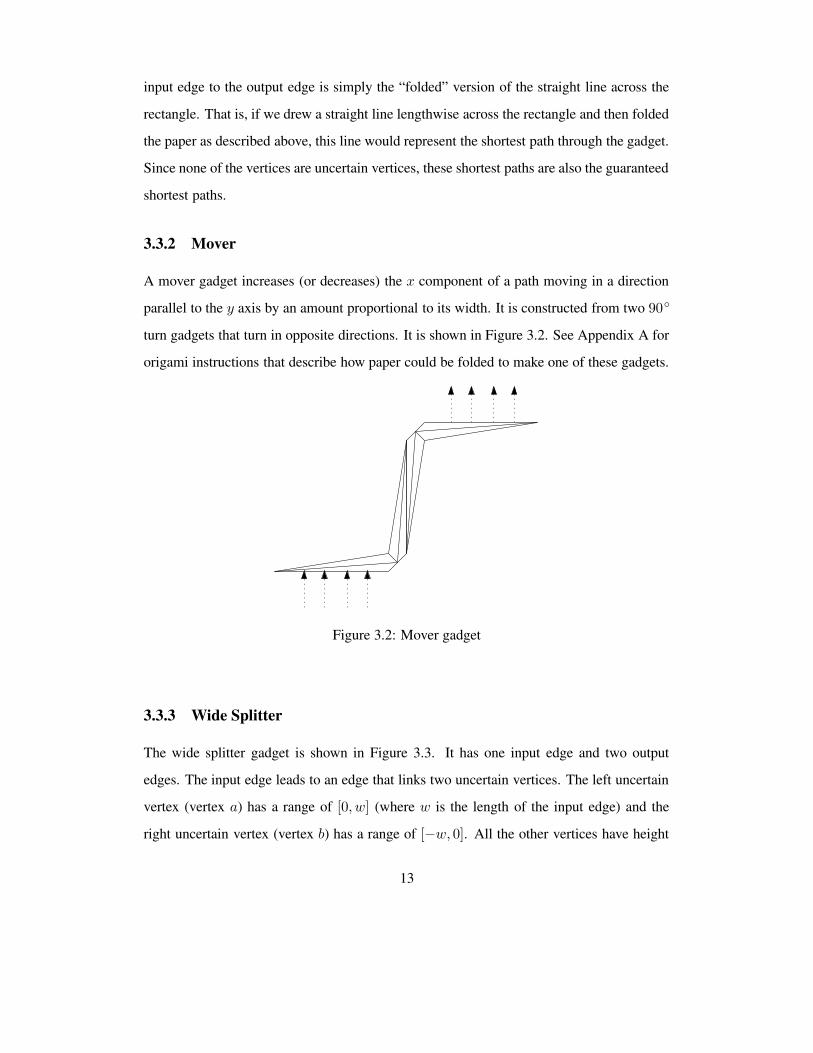
3.3.2 Mover

A mover gadget increases (or decreases) the x component of a path moving in a direction

parallel to the y axis by an amount proportional to its width. It is constructed from two 90◦

turn gadgets that turn in opposite directions. It is shown in Figure 3.2. See Appendix A for

origami instructions that describe how paper could be folded to make one of these gadgets.

Figure 3.2: Mover gadget

3.3.3 Wide Splitter

The wide splitter gadget is shown in Figure 3.3. It has one input edge and two output

edges. The input edge leads to an edge that links two uncertain vertices. The left uncertain

vertex (vertex a) has a range of [0, w] (where w is the length of the input edge) and the

right uncertain vertex (vertex b) has a range of [−w, 0]. All the other vertices have height

13

Input edge

Output edge Output edge

a b

c d

k l

ef

gh

j i

m

n o

Figure 3.3: Wide Splitter

0 except c and d, which have height w. The remainders of mover gadgets are attached to

each side of this contraption as shown.

We must show that any path P that travels through the correct part of the wide split-

ter as if it were a path through the appropriate version of the mover gadget is the guaranteed

shortest path through the splitter. That is, P is not only the shortest way through the splitter,

but the terrain is the worst possible for P .

Suppose the path leaves on the left output edge. When both uncertain vertices are

up, P is the shortest path across the gadget. Thus, if P is in its longest version on this

terrain, it is the guaranteed shortest path between these two points (since any other path is

longer at least on the terrain where both uncertain vertices are up). It remains to show that

the path is longest on this terrain. We will do this for the middle region of the input edge.

As a consequence of this analysis, we show exactly what we mean by “middle region.”

There are four cases to consider. When both uncertain vertices are up, the distance

function with respect to the entry point t on the input edge, is d(t) = 4w. See Figure 3.4.

When vertex a is down and vertex b is up, the distance function is d(t) = 2t + 2w, which

is less than 4w for all 0 ≤ t < w. See Figure 3.5. When both uncertain vertices are down,

the distance function is d(t) = 2t +√

2t2 + 2w. See Figure 3.6. This is less than 4w for all

14

0 ≤ t < 2w

2+√

2≈ 0.5857w. Finally, when vertex a is up and vertex b is down, the distance

function is

d(t) = |w − 2t| +√

t2 + ((w − t) − |w − 2t|)2 + w + 2w

This is less than 4w for all 0 ≤ t < 2w3 . See Figure 3.7.

a e

f g

h c

ji

k l = b

w

Figure 3.4: Wide splitter unfolded when a and b are up

If the path leaves on the right output edge, the limits are mirrored around t = w2

When both vertices are down, the distance function is d(t) = 4w. When vertex a is down

and vertex b is up, the distance function is d(t) = 2w − 2t + 2w, which is less than

4w for all 0 < t ≤ w. When both uncertain vertices are up, the distance function is

15

f g

h c

j i

b

Figure 3.5: Wide splitter unfolded when a is down and b is up

f g

h c

ji

bl

Figure 3.6: Wide splitter unfolded when a and b are down

16

a e

f g

h c

ji

k

l

b

m

n

Figure 3.7: Wide splitter unfolded when a is up and b is down. We have omitted triangleslbm and obn, which would cause intersections.

d(t) = (w − t) +√

2(w − t)2 + (w − t) + 2w, which is less than 4w for all w − 2w

2+√

2≈

0.41421w < t ≤ w. Finally, when vertex a is up and vertex b is down, the distance function

is

d(t) = |w − 2(w − t)| +√

(w − t)2 + ((w − (w − t)) − |w − 2(w − t)|)2 + w + 2w

This is less than 4w for all w3 < t ≤ w.

Thus, the middle region of the wide splitter is w − 2w

2+√

2< t < 2w

2+√

2.

3.3.4 Narrow Splitter

A narrow splitter simply takes the paths created by the wide splitter and uses mover gadgets

to move the paths so that every consecutive pair of paths have the same distance between

them. See Figure 3.8.

The width of the movers relative to the width, w, of the wide splitter is w + 2w

2+√

2−

w+δ2 . They are placed such that the tips of the output edges (as shown in Figure 3.8) are δ

apart.

17

Input edge

Output edge

Figure 3.8: Narrow Splitter

3.3.5 Shuffler

A shuffler is like a reversed narrow splitter except that the mover gadgets have a slightly

different width and the shuffler is slightly off-center with respect to the middle path entering

the input edge. This causes the paths from one half of the group of paths to interleave with

the other half.

For the shuffler, we describe the width and placement of the movers relative to the

output edge. The width of this edge is w. Let x0 and x1 be the endpoints of the range

of points that the paths are allowed to go through on the output edge and δ be the amount

of space between each portal on the input edge. Then the movers must each have width

w + x0−x1

2 − δ4 . They must be placed δ apart so that each directs exactly half of the paths.

We attach a wide collector to the output edges of the movers. In order for the portals

to interleave, we put the center of the wide collector δ2 units to the right of the center of both

of the movers.

18

Input edge

Output edge

Figure 3.9: Shuffler

3.4 Making Walls Non-vertical

As mentioned in Section 2.8, we have used vertical walls in some of the gadgets in order to

simplify the explanation of them. This is not legal, so we change the walls so that they are

very nearly vertical. This causes the portals to have nonzero width. We must ensure that the

portals do not become too large, otherwise it would be possible for a path to cross a gadget

in a “good” distance and end in a portal that does not correspond to the one it started in.

3.4.1 90◦ Turn

Suppose the 90◦ turn gadget is situated as shown in Figure 3.10. Then when we unfold it,

we get the quadrilateral pictured in Figure 3.11. Notice that one side is slightly longer than

the other, implying that the output edge is at a slight angle with respect to the input edge.

Therefore, shortest paths traveling from input to output edge vary in length depending on

where they start on the input edge.

We will not calculate the difference in the distance that paths travel because it turns

out to be unimportant. No 90◦ turn gadget is ever used on its own in our construction – they

are always used in pairs that turn in opposite directions. Doing this makes both edges have

19

the same length, which makes the output edge parallel to the input edge when the gadget

is unfolded. Therefore, while these gadgets used alone would cause the portals to widen,

when they are used in our construction, they do not.

(0, 0, 0)

(w, 0, 0)(w + ε, ε, w)

(w + 2ε, 2ε, 0)

(w + 2ε, w + 2ε, 0)

(w, 2ε, 0)

a bc

e

fd

Figure 3.10: 90◦ turn gadget with relative coordinates

a b

cd

ef

√

2ε2 + w2

√

2ε2 + w2

√

2ε2 + w2

√

w2 + 4ε2

√

w2 + 4ε2

w

w

Figure 3.11: 90◦ turn gadget unfolded

Wide Splitter

The wide splitter, on the other hand, does cause a slight widening of the portals since the

length to the output edge for paths entering on one side of the wide splitter is slightly more

than the length to the output edge for paths entering on the other side. The reason for this

is the small flat section just after the input edge. When the paths turn to the left, the flat

20

section is largest on the right side of the splitter. When they turn to the right, the flat section

is largest on the left side. Since the paths can only enter on the middle region of the wide

splitter, the difference between the length of the shortest locally optimal path that travels

through the splitter and the longest locally optimal path that travels through the splitter is

less than (√

2γ +√

w2 + 2γ2 + 2γw −√

w2 + 4γ2)/3 (see Figure 3.12). We can upper-

bound this value by (√

2γ + 2γ)/3.

If we let the length of the path across the splitter be the length of the longest possible

locally optimal path, then the length allowed across the splitter is l = 2√

w2 + 2γ2 +

2√

w2 + 4γ2 +(2(2+√

2)γ)/3. The base of the right triangle with l as its hypotenuse and

l − (√

2 + 2)γ/3 as its height is√

(2 +√

2)γ

3(4

√

w2 + 2γ2 + 4√

w2 + 4γ2 + (2 +√

2)γ)

Therefore, if γ ≤ ε2

4(2+√

2)√

w2+1, each portal can increase in width by at most 2ε.

√

2γ

√

w2 + 2γ2 + 2γw

√

w2 + 4γ2

√

w2 + 2γ2

√

w2 + 2γ2

w

w

Figure 3.12: Wide splitter gadget unfolded. We attach an unfolded 90◦ turn gadget to thetop, with the long side of that gadget attached to the short side of the splitter.

Since the rest of the gadgets are created from the wide splitter (as well as movers),

there is nothing else that can cause the portals to widen. We can make portals start very far

apart in the first splitter (a polynomial number of bits gives us a lot of room to work with),

so portals will not overlap at any point in our construction. Thus we have sketched a proof

21

to

Theorem 3.1. The guaranteed shortest path problem is NP-hard. That is, we can find a

path that has length ≤ K if and only if we can find a setting of variables that satisfies the

formula Φ in 4-CNF form.

22

Chapter 4

Optimistic Shortest Paths

4.1 Introduction

The assumption that the terrain will be the worst possible for any path is not a cheery one,

and Alice is a cheery girl. She decides that she is going to find the shortest path to Bob’s

house under the assumption that the terrain is going to be the best for any path that she

chooses.

Notice that, unlike with guaranteed shortest paths, we must consider the infinitude

of possible terrains when we are deciding which terrain is the best for each path. For

example, if it is possible for the uncertain vertices to be situated so that the terrain appears

to be perfectly flat from the path’s point of view, then we will assume that the vertices are

at these elevations.

4.1.1 Problem Statement

Given an uncertain terrain and two points s and t in the xy-plane, we want to find a path

from s to t that has the shortest length among all paths from s to t where the path length

is measured on the consistent terrain that minimizes its length. Cast as a decision problem,

this becomes, “Is there a path from s to t on some consistent terrain of length at most K?”

We call this the optimistic shortest path since we are measuring a path on the consistent

23

terrain that minimizes its length.

4.2 The Construction

4.2.1 Rotator

A basic operation that our gadgets must perform is to rotate the orientation of the group of

portals by 90◦ in the xz plane. This is important as a building block of other gadgets and is

performed by a rotator, which is like a square of paper folded along its diagonal. See Figure

4.1 for an example of a rotator of width 1 located at (0, 0, 0) with a thickness parameter γ

that is essentially 0. Note that vertex d is an uncertain vertex. Any path that enters this

gadget at (x, 0, 0) is shortest if it goes vertically up from its input edge to the diagonal edge

and then horizontally from there to the vertex d, which is at height x (approximately – see

Lemma 4.1 for a more precise discussion).

(0, 0, 0)(1, 0, 0)

(1, γ, 1)

Input Edgea

c

b

Front View

Output Vertex

Back View

a

c

b(1, 2γ, [0, 1])

dd

Figure 4.1: Front and back view of a rotator showing shortest paths across it as dotted lines

Since the shortest paths leave the rotator in a vertical line, we have changed the

orientation of the line of portals from horizontal to vertical.

4.2.2 Path Splitter

To create the splitter, shown in Figure 4.2, we construct the uncertain terrain so that any

shortest path from s to t must enter at or near the uncertain vertex d, cross either edge ef or

fg, and cross output edge eg. The height of the input vertex d closely determines the point

at which the path crosses the output edge.

24

Note that splitters are like two rotators that have been joined together.

Output Edge

Input Vertex

(2, γ, 0)(0, γ, 0)

(1, γ, 1)

(1, 0, [0, 1])

Front View

Back View

e

f

gd

eg

f

Figure 4.2: The splitter, showing the doubling of the number of path classes

4.2.3 Creating Portals

Given these gadgets, we are ready to describe the first part of the construction. In front of

the initial point s, we construct a splitter that is high enough that any shortest path from s

to t must go around the wall to the left or right. This creates two portals. Following this

wall is a sequence of n connected rotators and splitters, joined at their common vertex d

and increasing in size by a factor of 2 each time. When we join the rotators and the splitters

at the vertex d, we leave a gap between vertex a on the rotator and vertex e on the splitter

that cannot be crossed. (See section 2.7).

The output edge of the last splitter may be reached from s via 2n shortest routes.

Each of these shortest routes intersects the final output edge at a different location along the

output edge. We number the resulting portals along this edge from 0 to 2n−1 and associate

them with the 2n possible truth assignments to the variables of the formula Φ. The rest of

the construction lengthens the paths in those portals that correspond to unsatisfying truth

assignments.

25

4.2.4 Path Shuffler

As with the splitter, the shuffler can be seen as being composed of two rotators put together.

Assume that the paths are δ apart. We will split the group of paths into two parts, so that

half go to one side and half go to the other. When the group has been split, one of the halves

will be raised by (w/2 + δ/4, where 2w is the width input edge) and the other half will be

lowered the same amount. The paths will then be rotated so that they interleave vertically.

We put a gap between the two groups of paths. This is shown in Figure 4.3 as the

gray triangle.

The shortest paths leave the rotators through point a or point b in Figure 4.3. They

then travel along edge ac or bc to point c. Point c is the input vertex to a reversed rotator

(not shown) that rotates the group of paths back to horizontal.

(1, 1, 0)

(2, 0, 0)(0, 0, 0)

(0, 2,− 1

2− δ

4) (2, 2, 1

2+ δ

4)

(1, 2 + 3γ, [−1/2− δ/4, 1/2 + δ/4])

(0, 1, 0) (2, 1, 0)

0123

0 1 2 3 4 5 6 7

7654

a bc

Input Edge

Figure 4.3: The shuffler viewed from above. The circled regions contain rotators, shownprojected into the xz plane above the shuffler at the correct relative heights. The vertexmarked c is the output vertex.

Using the gadgets described in this section, we construct the splitters following the

26

procedure outlined in Chapter 2. That is, we construct the literal filters using n shufflers

and a barrier, then we construct clause filters using four literal filters, and finally we make

formula filters by putting the clause filters in series. As before, we must make sure that

portals do not overlap.

4.3 The Hardness of Optimistic Shortest Paths

We will now show that each gadget increases the length of the shortest path traveling

through it by a specified amount. We will also show that a shortest path must traverse

each gadget in a locally optimal fashion. That is, if it enters a gadget via input portal i it

must exit via a corresponding output portal.

Lemma 4.1. For a rotator of width w, there exists a path from a point in ([x0, x1], 0, 0) on

the input edge to the output vertex of length less than or equal to w + 2γ only if the path

exits through the output vertex in the range (w, 2γ, [x0 − ε, x1 + ε]) where γ = ε2

8w.

a b

c

w

√

w2 + γ2

Figure 4.4: The unfolding has three fixed vertices and the fourth inside the shaded strip.

Proof. In order to find the locally optimal path across a rotator, first we consider the unfold-

ing of the rotator when the output vertex is at its lowest possible elevation and γ = 0. The

27

shortest path from the point (x0, 0, 0) is clearly the straight line across to (x0, w, 0). If we

refold the rotator, this point goes to (w, 2γ, x0). Since points can only exit via the output

vertex, the output vertex must move to that point.

Now consider the case when γ 6= 0. Whereas the unfolding of the rotator was a

square with edge length w, it is now a quadrilateral. In the unfolding (see Figure 4.4), the

triangle abc forms a right-angled triangle with leg lengths w and√

w2 + γ2. The fourth

vertex d falls within a strip of width γ above the w×√

w2 + γ2 rectangle. We can construct

an approximation of the quadrilateral that is a w×w square with a 2γ strip added to the top

to represent the uncertain location of d; the output vertex d must be inside this strip.

If we consider a path of length w + 2γ across this quadrilateral from an arbi-

trary input point, the width of the region that the output point could potentially be in is

4√

γ(w + γ) (the length of the chord at distance w from the input point in a circle centered

at the input point of radius w + 2γ). Therefore, if γ = ε2

8w, this region has a width that

is less than 2ε. Thus, if the input point starts in range [x0, x1], it will exit in the range

[x0 − ε, x1 + ε].

Lemma 4.2. For a shuffler of width 2w, there exists a path from a point in ([x0, x1], 0, 0) on

the input edge to the output vertex of length less than or equal to 2w+√

w2 + (w/2 + δ/4)2+

2γ only if the output vertex is either in (w, 2w+3γ, [x0−w/2−δ/4−ε, x1−w/2−δ/4+ε])

or in (w, 2w + 3γ, [x0 +w/2 + δ/4− ε, x1 + w/2 + δ/4 + ε]), depending whether x1 < 1

or not.

Proof. The locally optimal motion for a path entering a shuffler in a straight line in the

vertical projection to the rotator across from it. Once it is at the rotator, Lemma 4.1 applies.

From Lemma 4.1 and Lemma 4.2, we can deduce the maximum distance possible

for any locally optimal path that corresponds to a truth assignment that satisfies the formula

Φ. This distance will always be less than the minimum distance of any path that is either not

locally optimal or that corresponds to a truth assignment that does not satisfy the formula Φ.

28

We ensure that no path crosses from a portal representing one truth assignment to a portal

that represents another by making the initial wall very wide. This creates a large initial

separation between portals. Since the width of a portal only grows by 2ε for each gadget,

the portals are always separated by enough so that any path that goes from an input portal to

a non-corresponding output portal is too long to satisfy our optimistic shortest path length

bound. Thus we have

Theorem 4.1. The optimistic shortest path problem is NP-hard. That is, we can find a path

that has length ≤ K if and only if we can find a setting of variables that satisfies the formula

Φ in 4-CNF form.

29

Chapter 5

Conclusions

We have outlined two proofs showing that finding a shortest path on uncertain terrains given

the optimistic and pessimistic assumptions are a hard problems. The method used to prove

that these problems are hard has been shown to be useful and fairly generalizable.

5.1 Open Problems / Future Work

One natural problem arising from the results presented here is to find an ε-approximation

algorithm that solves the guaranteed and optimistic shortest path problems with a path that

is no longer that (1 + ε) times the length of the shortest path. These algorithms exist (with

a running time inversely proportional to ε) for the 3D Euclidean shortest path [5] and for

the d1-optimal motion of a rod [1] problems – problems which have hardness proofs very

similar to those that were shown.

The “discrete” case of the guaranteed shortest path and optimistic shortest path

problems is the same problem with the restriction that the paths must travel on edges of the

terrain. In the guaranteed shortest path case, the fact that vertices only need to be considered

at extreme elevations implies that this can be turned into a very manageable graph. It might

be that this will allow a polynomial algorithm to be found.

Another interesting area for future work would be to look at possibility of using

linear programming to solve these problems in the L1 (Manhattan) metric. This type of

30

solution does not work in the L2 (Euclidean) metric because of the square roots and the

square operations in the distance measurements.

Exploring other geometric problems like the Voronoi diagram or the convex hull

problem on uncertain terrains might also be interesting, but seem like they would almost

certainly be NP-hard. This is because many of these problems depend on being able to find

the shortest path between points in a reasonable amount of time and we have just shown

that this is not likely to be possible.

31

Bibliography

[1] Tetsuo Asano, David Kirkpatrick, and Chee K. Yap. d1-optimal motion for a rod.

In Proceedings of the Twelfth Annual Symposium On Computational Geometry (ISG

’96), pages 252–263, New York, May 1996. ACM Press.

[2] Chanderjit Bajaj. The algebraic degree of geometric optimization problems. Discrete

Comput. Geom., 3(2):177–191, 1988.

[3] John Canny and John Reif. New lower bound techniques for robot motion planning

problems. In Ashok K. Chandra, editor, Proceedings of the 28th Annual Symposium

on Foundations of Computer Science, pages 49–60, Los Angeles, CA, October 1987.

IEEE Computer Society Press.

[4] Jindong Chen and Yijie Han. Shortest paths on a polyhedron. In Proceedings of the

sixth annual symposium on Computational geometry, pages 360–369. ACM Press,

1990.

[5] Joonsoo Choi, Jurgen Sellen, and Chee-Keng Yap. Approximate euclidean shortest

path in 3-space. In Proceedings of the tenth annual symposium on Computational

geometry, pages 41–48. ACM Press, 1994.

[6] Edsger W. Dijkstra. A note on two problems in connexion with graphs. Numer. Math.,

1:269–271, 1959.

[7] M. R. Garey and D. S. Johnson. Computers and Intractability: A Guide to NP-

Completeness. W.H. Freeman and Company, San Francisco, California, 1979.

32

[8] Chris Gray and William Evans. Optimistic shortest paths on uncertain terrains. In

Proceedings of the 16th Canadian Conference on Computational Geometry, 2004.

[9] Sanjiv Kapoor. Efficient computation of geodesic shortest paths. In ACM, editor, Pro-

ceedings of the thirty-first annual ACM Symposium on Theory of Computing: Atlanta,

Georgia, May 1–4, 1999, pages 770–779, New York, NY, USA, 1999. ACM Press.

[10] Joseph S. B. Mitchell. Geometric shortest paths and network optimization. In Hand-

book of Computational Geometry, J.-R. Sack, and J. Urrutia, editors, Elsevier, 2000.

2000.

[11] Joseph S. B. Mitchell, David M. Mount, and Christos H. Papadimitriou. The discrete

geodesic problem. SIAM J. Comput., 16(4):647–668, 1987.

[12] Micha Sharir and Amir Schorr. On shortest paths in polyhedral spaces. SIAM Journal

on Computing, 15(1):193–215, February 1986.

33

Appendix A

Origami Instructions

The following instructions are for making the mover gadget described in Chapter 3. All of

the other gadgets in Chapter 3 are compositions of this gadget, so it can be used to make

any of them.

34

1. Start with a 1 × 4 strip of paper.

2. Fold right corner up to the top edge.

3. Fold the rest of the strip up.

4. Fold the top part of the strip over to make the pictured triangle.

5. Fold the leftmost part of the strip into the final triangle.

6. Fold the top half over onto the bottom half.

7. To finish, fold the right quarter and the left

quarter until they are at right angles with the

middle half.

35