Shorting in Speculative Markets∗

Marcel Nutz† José A. Scheinkman‡

March 28, 2018

Abstract

We propose a continuous-time model of trading with heterogeneousbeliefs. Risk-neutral agents face quadratic costs-of-carry on positionsand thus their marginal valuation of the asset decreases with the sizeof their position, as it would be the case for risk-averse agents. In theequilibrium models of heterogeneous beliefs that followed the work byHarrison and Kreps, investors are risk-neutral, short-selling is prohib-ited and agents face constant marginal costs of carrying positions. Theresulting resale option guarantees that the equilibrium price exceedsthe price of the asset in a static buy-and-hold model where speculationis ruled out and this difference is identified as a bubble. Our modelfeatures three novelties to this literature. First, increasing marginalcosts entail that the price depends on asset supply. Second, in ad-dition to the resale option, agents also value an option to delay, andthis may cause the market to equilibrate below the buy-and-hold price.Third, we introduce the possibility of short-selling. Our model showsthat when shorting is very costly, price formation is dominated by op-timists and pessimists’ views are hardly reflected. On the other hand,an unexpected decrease in shorting costs may lead to the collapse ofa bubble; this links the financial innovations that facilitated shortingof mortgage backed securities to the subsequent collapse of prices rel-ative to fundamentals. We use a Hamilton–Jacobi–Bellman equationof a novel form to describe the equilibrium of our model and derivecomparative statics results.

1 Introduction

As Kindleberger and Aliber (2005) elaborate, many classical economists ar-gued that the purchase of securities for re-sale rather than for investmentincome was the engine that generated numerous historical asset price bub-bles. To explain such speculation in a dynamic equilibrium model, Harrison∗We are indebted to Pete Kyle and Xunyu Zhou for fruitful discussions. An earlier

version was titled “Supply and Shorting in Speculative Markets.”†Columbia University. Research supported by an Alfred P. Sloan Fellowship and NSF

Grant DMS-1512900.‡Columbia University, Princeton University and NBER.

1

and Kreps (1978) study risk-neutral agents with fluctuating heterogeneousbeliefs. In their model, long positions can be financed at a constant interestrate and short-selling is ruled out. The buyer of an asset thus acquires botha stream of future dividends and an option to resell which in combinationwith fluctuating beliefs guarantees that speculators are willing to pay morefor an asset than they would pay if they were forced to hold the asset tomaturity; that is, risk-neutral investors would pay to be allowed to specu-late. Scheinkman and Xiong (2003) added trading costs and showed thatthese models generate a correlation between trading volume and overpric-ing,1 a characteristic of several of the major bubble episodes in the last threecenturies.2

Another stylized fact is that bubble implosions often follow increases insupply. For instance, the implosion of the dotcom bubble was preceded bya vast increase in the float of internet shares.3 The South Sea bubble lastedless than one year, but in that period the amount of outstanding shares of theSouth Sea Company more than doubled, and many other joint-stock com-panies were established.4 However, the assumption of risk-neutral investorsfacing constant marginal costs in the earlier literature on disagreement andbubbles implies that supply is irrelevant for pricing.5 Hong et al. (2006)analyzed a two-period model with risk-averse investors where unexpected in-creases in supply could deflate bubbles. The economics is straightforward—when agents are risk-averse, their marginal valuation for a risky asset de-creases with the amount they hold.

Short-selling an asset can be seen as a source of additional supply. Thecollapse of prices for mortgage backed securities in 2007 was preceded bya series of financial innovations that facilitated shorting: the creation of astandardized CDS for MBS in 2005, the introduction of traded indexes forsubprime mortgage backed credit derivatives in 2006, and the use of CDSto construct synthetic CDOs that allowed Wall Street to satisfy the global

1See also Berestycki et al. (2016).2See e.g. Carlos et al. (2006) on the South Sea bubble, Hong and Stein (2007) on

the Roaring Twenties, Ofek and Richardson (2003) and Cochrane (2002) on the internetbubble, Xiong and Yu (2011) on the Chinese warrant bubble.

3See Ofek and Richardson (2003).4The directors of the SSC understood that the bubble companies competed with the

SSC’s conversion scheme and could deflate its own bubble. Harris (1994) documents thatthe Bubble Act of 1720, which banned joint-stock companies except if authorized by RoyalCharter, was produced at the behest of the company to limit the competition for capital.

5Except for the assumption of positive net supply, issues concerning supply of the assetsubject to bubbles are also ignored in the rational bubbles literature (Santos and Woodford(1997)).

2

demand for US AAA mortgage bonds without going through the relativelyslow process of building new housing.6 These innovations allowed pessimiststo profit from the excessive optimism prevailing among CDO buyers.7 Theamounts shorted were substantial; Cordell et al. (2011) estimate that syn-thetic CDOs, mostly issued after 2005H2, more than doubled the amount ofBBB tranches of Home Equity Bonds placed in CDOs during 1998–2007.8 Itis unlikely that this supply would have been absorbed without any price im-pact. In any case, starting in the second half of 2007, prices seem to exhibitsubstantial discounts relative to fundamentals.9

We propose a model with a population of investors trading a single assetand aiming to maximize expected cumulative net gains from trade. These in-vestors are risk-neutral and have fluctuating heterogeneous beliefs, includingpossibly beliefs about future changes in supply. In contrast to the previ-ous literature, shorting is allowed, albeit at a higher cost when compared togoing long: holders of short or long positions pay costs which are propor-tional to the square of their positions.10 The two constants of proportionalitymay be different; this asymmetry between costs of going short and long isa well-known feature of financial markets, see e.g. D’Avolio (2002)11, andthe assumptions in the earlier literature correspond to an infinite cost forshort positions and zero cost for long positions. On the one hand, the costsin our model reflect monetary costs of holding a long position (in particularincreasing costs of capital) or borrowing stocks to establish a short position.On the other hand, they stand in for risks that we do not explicitly model,such as market-wide liquidity shocks that would force agents to liquidate

6See Scheinkman (2014) for a summary or Lewis (2015) for an excellent detailed ac-count.

7Foote et al. (2012) lay out 12 facts about the mortgage market during the boomyears and argue persuasively that “any story consistent with the 12 facts must have overlyoptimistic beliefs about house prices at its center.”

8For instance, Abacus 2007-AC1, the synthetic CDO made infamous by the SEC en-forcement action against Goldman Sachs, was composed of CDS totaling $2 billion. Theoriginal cash value of the underlying BBB bonds was $1.238 billion (Cordell et al. (2011)).BBB tranches of Home Equity Bonds were an essential fuel to the CDO machine thattransformed subprime mortgages into AAA rated bonds.

9Beltran et al. (2017) attribute the low prices to the increase in asymmetric informationbetween buyers and sellers that followed the downgrades of MBS securities by ratingagencies in summer 2007. Analyzing the pricing of index credit default swaps post-crisis,Stanton and Wallace (2011) suggest that the pricing reflected a limited supply of insuranceof asset backed securities, presumably relative to demand.

10For tractability, we assume that costs are a function of the size rather than the valueof the position.

11Some of this asymmetry refers to costs which are linear on positions; we treat thesedifferences in Appendix B.

3

their positions at unfavorable prices or the recall risk faced by short sell-ers. Indeed, since costs are quadratic, an agent’s marginal valuation of theasset will decrease as their position increases, as it would be the case forrisk-averse agents. Thus we view our setup as an alternative to a much lesstractable model with risk aversion, with many of the same forces present. Inparticular, we show below that an increase in aggregate supply of the assetlowers equilibrium prices.

Importantly, using the cost coefficients as parameters allows us to studythe impact of market frictions on prices. Theorem 2.1 reveals precisely howthese costs amplify or diminish the impact of optimists’ and pessimists’ views(see Remark 2.2). In particular, we detail in Section 3.2.2 that when the costof shorting is prohibitively high, the equilibrium is determined by optimistssince pessimists cannot speculate, thus leading to inflated prices. Dietheret al. (2002) provide evidence that stocks with higher dispersion in analysts’earnings forecasts earn lower future returns than otherwise similar stocks;this is consistent with the hypothesis that the relatively higher costs of short-ing make prices reflect the more optimistic opinions.12 On the other hand,Example 4.9 illustrates that an unexpected decrease of the cost of shortingcan lead to a collapse of an asset price bubble, thus rationalizing a link be-tween the decrease of the cost of shorting in the MBS market in 2005–07 andthe collapse of CDO prices relative to fundamentals.

A buyer of the asset today may forecast that at some future date shewould be able to sell at a price that would exceed her own valuation of theasset at that date. Because of this resale option, she may be willing to paymore than what she believes is the discounted value of the payoff of an asset.In the classical models, this option causes equilibrium prices to exceed theprice that would prevail if re-trading is ruled out—we call the latter thestatic price for brevity. In addition, there is also an option to delay whichhas not been highlighted in the earlier literature on heterogeneous beliefs. Aspeculator that buys y units today may plan to buy additional units of theasset in future states of the world where there would be a larger differencebetween the asset price and her marginal valuation for the asset if she holdsy units. However, if the cost of holding a long position is zero, this delayoption has no impact in equilibrium. The intuition is that, since agentsare risk-neutral and there is no cost-of-carry, a buyer of the asset must beindifferent as to the amount of the asset she buys. Hence, the delay optionhas no value, and in particular, the dynamic equilibrium price cannot be

12Moreover, it is inconsistent with a view that dispersion in analysts’ forecasts proxiesfor risk.

4

smaller than the static price. In Example 4.6 we show that in the presenceof a positive cost, the option to delay may outweigh the resale option andcause the dynamic price to be lower than the static one, even when shortingis prohibited.

When shorting is allowed, the short party also has the correspondingoptions. An agent that acquires a short position today may forecast that atsome future date he would be able to repurchase the asset at a price thatwould be below his own valuation at that date. This option to resell a shortposition, that is the option to cover shorts, in turn, decreases the minimumamount pessimists would be willing to receive for shorting the asset, puttingdownward pressure on prices. The short party also enjoys an option to delay.In Example 4.9 we show that when the cost of holding a short position is closeto the cost of holding a long position, the equilibrium price may be less thanthe static price. We argue that this happens because the long party valuesthe resale option less than the short party values the repurchase option.

1.1 Other Related Literature

In a pioneering paper allowing for short-sales and risk aversion in a continuous-time setting of heterogeneous beliefs, Dumas et al. (2009) consider a completemarkets model with two classes of agents, one of which is overconfident abouta public signal. Overconfident-investors’ reaction to the signal introduces arisk factor—sentiment risk—which carries a risk-premium and causes stockprices to be excessively volatile. In their model, the delay option must bevaluable and supply affects equilibrium prices, but these questions are notexplicitly analyzed. Instead, Dumas et al. (2009) focus on the importantquestion of identifying the trading strategy that would allow a rational in-vestor to take advantage of excessive stock price volatility and sentimentfluctuations and show that rational investors choose a conservative portfoliothat is sensitive to their predictions about future realization of sentiment.Dumas et al. (2009) assume a cost symmetry between going short and long(the short party receives the equilibrium price and must pay the dividendsthat accumulate until the position is closed) so one cannot examine the effectof changes in shorting costs.

The literature on asset pricing with search frictions that follows Duffieet al. (2005) assumes that agents have fluctuating private benefits from hold-ing an asset and that opportunities for trading are randomly distributed.Strict concavity of private benefits implies that the supply of the asset af-fects equilibrium prices. Our assumption of quadratic costs of holding aposition could be similarly motivated as private benefits (but in our case

5

the differences come from heterogeneity of beliefs rather than benefits). Thefluctuating private benefits also generate options to resell and to delay trad-ing which are discussed in Lagos and Rocheteau (2006), Feldhütter (2012)and Hugonnier et al. (2014). These authors point out that depending onthe curvature of private benefits an increase in trading opportunities maydecrease or increase the price of the asset. In particular the comparison be-tween prices that would prevail when re-trading opportunities are more orless frequent is ambiguous. However, short-selling, changes in shorting costs,or the impact of increases in aggregate supply are not emphasized in thisliterature.

1.2 Overview

In Section 2 we describe in detail a continuous-time model where n types ofagents trade a single asset. The agents disagree on the future evolution of aMarkov state whose time T value determines the asset’s payoff. In equilib-rium, they find a price process for the asset, given by a function of time andMarkov state. Types that expect prices to increase on average over the nextinstant choose to go long, where the amount they go long depends on their ex-pected price changes and the cost of carrying long positions. The other typeschoose to go short, by amounts that depend on their expected price changesand the cost of carrying short positions. Equilibrium requires that the longsabsorb the shorts plus an exogenous supply. Theorem 2.1 shows that thereis a unique equilibrium price function and that it can be characterized bya partial differential equation (PDE). This equation is of Hamilton–Jacobi–Bellman-type with a novel form where the optimization runs over the waysto divide the agents into two groups at any time and state; at the optimum,these are the optimists (holding long positions in equilibrium) and the pes-simists (holding shorts). The price can also be seen as the value function ofa stochastic optimal control problem (Proposition 2.4) where the controllerchooses among a set of laws of motion; this is useful for the derivation ofour subsequent results. Thus, the equilibrium of our model is remarkablytractable despite the general form of beliefs. An economic interpretation ofthe PDE is given by the solution to a problem of a planner with limitedinstruments who tries to maximize the initial price (Theorem 2.5). In eitherproblem, a noteworthy feature is that the supply enters mathematically asa running cost (i.e., like intermediate consumption in Merton’s problem).

In Section 3 we provide several comparative statics and limiting results.In particular, we show that an increase in supply decreases the equilibriumprice and that a decrease (increase) in the cost for long (short) positions

6

increases the price. We also establish that as the cost for long positionsconverges to zero, the equilibrium price function converges to a functionthat does not depend on the cost of holding a short position or the amountsupplied. Thus, the crucial assumption in the earlier literature is not thatshorting is impossible, but that the marginal cost of carrying long positionsis constant. On the other hand, as the cost of shorting becomes prohibitive,the equilibrium price converges to a function that does depend on the costof carrying long positions as well as the exogenous supply of the asset.

In Section 4 we discuss the impact of speculation in our model. To thatend, we first characterize the static equilibrium price; that is, the price thatprevails when re-trading is not allowed and agents are forced to use buy-and-hold strategies. Then we compare this static price with the dynamic one(where re-trading is possible) and in particular we provide examples thatillustrate the effect of the resale and delay options, both when shorting isruled out and when shorting is allowed. The difference between the dynamicprice and the static price has been identified as the size of the bubble inthe previous literature. With this identification, the examples in this sectioncan be used to illustrate that, in the presence of increasing marginal costs-of-carry, lowering the cost for shorts or increasing the cost for long positionscan lead not only to a bubble implosion but even to a negative bubble.

The concluding remarks are stated in Section 5 and the proofs for ourresults in Sections 2–4 are reported in Appendix A.

The assumption that costs are proportional to the square of the posi-tion does not accommodate the fact that borrowers of stock typically pay afee quoted as an annualized percentage of the value of the loaned securities(the rebate rate). This assumption is made to simplify the exposition andallow us to concentrate on the effects of the size of a position on an agent’smarginal valuation. In Appendix B we discuss how our results can be gener-alized if an additional linear term is added to the costs-of-carry. The agentsare then divided into three rather than two groups: while strongly optimisticand pessimistic agents hold long and short positions, respectively, an inter-mediate group expects that prices will not move enough to compensate forthe first-order costs and stays out. However, the qualitative properties ofequilibria remain the same as without the linear term, so we have chosento use the simpler model in the body of the paper. We also examine inAppendix C how the model changes if costs of going long and/or short varyacross agents. While the structure of the equilibrium remains similar, ceterisparibus, agents with lower costs take larger positions and have a larger influ-ence on the coefficients of the PDE that determines the equilibrium price.

7

2 Equilibrium Price

In this section, we detail our formal setup and show that it leads to a uniqueequilibrium. The corresponding price is described by a partial differentialequation which, in turn, leads us to a stochastic control problem. Finally,an economic interpretation for the latter is provided through a planningproblem.

2.1 Definition of the Equilibrium Price

We consider n ≥ 1 types, each with a unit measure of agents, who trade asecurity over a finite time interval [0, T ]. For brevity, we will often refer to atype as an agent. The security has a single payoff f(X(T )) at the horizon,where f : Rd → R is a bounded continuous function and X is the stateprocess. While there is no ambiguity about f , the agents agree to disagreeon the evolution of the state process. Mathematically, we take X to be thecoordinate-mapping process on the space Ω = C([0, T ],Rd) of continuous,d-dimensional paths, equipped with the canonical filtration and sigma-field.The view of agent i is represented by a probability measure Qi on Ω underwhich X follows the stochastic differential equation (SDE)

dX(t) = bi(t,X(t)) dt+ σi(t,X(t)) dWi(t), X(0) = x, (2.1)

where Wi is a Brownian motion of dimension d′ and the functions

bi : [0, T ]× Rd → Rd, σi : [0, T ]× Rd → Rd×d′

are deterministic. We assume13 throughout that (the components of) biand σi are in C1,2

b , the set of all bounded continuous functions g : [0, T ] ×Rd → R whose partial derivatives ∂tg, ∂xig, ∂xixjg exist and are continuousand bounded on [0, T ) × Rd. Moreover, we assume that14 σ2

i is uniformlyparabolic; that is, its eigenvalues are uniformly bounded away from zero.These conditions imply in particular that the SDE (2.1) has a unique (strong)solution.

Notice that we allow for the differences in beliefs to affect both driftand diffusion coefficients. While much of the literature on disagreement inasset markets deals with constant volatility processes and thus naturallyassumes that disagreement concerns only drifts, there is plenty of evidence

13These conditions could be relaxed considerably. The present form allows for a simpleexposition avoiding issues of technical nature.

14 Given a matrix A, we write A2 for the product AA> of A with its transpose A>.

8

that more complex processes involving stochastic and time-varying volatilityare necessary to understand empirical features of asset prices. In this context,it is quite plausible that agents may also differ in their forecasts15 for thevolatility.

Agents trade the security throughout the interval [0, T ], at a time t priceP (t) to be determined in equilibrium. The agents are subject to an instan-taneous cost-of-carry c which is different for long and short positions,

c(y) =

1

2α+y2, y ≥ 0,

12α−

y2, y < 0.(2.2)

Here the (inverse) cost coefficients α± are given constants satisfying

0 < α− ≤ α+,

meaning that the cost of shorting is higher than the cost of going long. Anadmissible portfolio Φ for an agent is a bounded16, progressively measurableprocess, and we write A for the collection of all these portfolios. The valueΦ(t) indicates the number of units of the security held by the agent at time t,and this number can be negative in the case of a short position. Given a(semimartingale) price process P , agent i seeks to maximize the expectednet payoff17

Ei

[∫ T

0Φ(t) dP (t)−

∫ T

0c(Φ(t)) dt

]; (2.3)

here the first integral represents the profit-and-loss from trading and thesecond integral is the cumulative cost-of-carry incurred. Criterion (2.3) canbe rationalized by assuming that agents have access to borrowing and lend-ing at a zero interest rate and that the cost function c is measured in theunit of account but it can also be taken as a primitive utility function.18

15Note that while the past trajectory of σ(t,X(t)) can be inferred from the observationof X(t), agents may very well differ in their forecasts. This is obvious if σ depends ontime t, but even if not, the past observation of σ(t,X(t)) will typically reveal little ofthe function σ when X is non-recurrent (e.g., of dimension larger than 2). We will seein Theorem 2.1 that the pricing of the security indeed depends on the future volatilityover the entire time interval. This is quite natural as the same would be true in standardrisk-neutral pricing when f is a derivative on a stock, for instance.

16 Boundedness could be replaced by suitable integrability conditions without alteringour results.

17 To ensure that the expectation is well-defined a priori, we set Ei[Y ] := −∞ wheneverEi[min0, Y ] = −∞, for any random variable Y . For the processes P that occur in ourresults below, (2.3) will be finite for any Φ ∈ A.

18By adding notation we could accommodate a constant non-zero interest rate or dis-count rate.

9

An admissible portfolio Φi will be called optimal for agents of type i if itmaximizes (2.3) over all Φ ∈ A. We will examine symmetric equilibria inwhich agents of the same type choose the same portfolio.

As the final input of our model, we introduce a nonnegative, progressivelymeasurable process S representing exogenous supply. The latter is ownedby third parties that supply their endowment inelastically.19 We assumethat S(t) = s(t,X(t)) for a deterministic and nonnegative supply functions ∈ C1,2

b .20 Let P be a continuous, progressively measurable process whichis a semimartingale with P (T ) = f(X(T )) a.s. under all Qi. We say that Pis an equilibrium price if there exist admissible portfolios Φi, i ∈ 1, . . . , nsuch that Φi is optimal for agent i and the market clearing condition

n∑i=1

Φi(t) = S(t)

holds. We are interested in Markovian equilibria; that is, equilibrium pricesof the form P (t) = v(t,X(t)) for a deterministic function v which we referto as an equilibrium price function.

2.2 Existence and PDE for the Equilibrium Price

The following notation will be useful to state our first result. Given v ∈ C1,2b ,

we define the function Liv by

Liv(t, x) = ∂tv(t, x) + bi∂xv(t, x) +1

2Trσ2

i ∂xxv(t, x).

Here ∂xv denotes the gradient vector, ∂xxv the Hessian matrix, and Trσ2i ∂xxv

is the trace of the matrix σ2i ∂xxv; that is, the sum of the entries on the

diagonal. Finally, for a subset I ⊆ 1, . . . , n, we denote by Ic = 1, . . . , n\Ithe complement and by |I| the number of elements in I.

Before stating the characterization of equilibria it is worthwhile to ex-amine the homogeneous case where all agents have the same views, rep-resented by coefficients bi = b and σi = σ. Thus, Liv(t, x) = Lv(t, x)is also independent of i. The quadratic costs imply that the optimal po-sitions are unique and identical across agents; in particular, there is noshort-selling in equilibrium. Positions are determined by the first-order

19Since the utility function in (2.3) is separable, the equilibrium price is invariant toendowments. Hence, we could have alternatively assumed an arbitrary ownership structurefor the endowment across the types of investors—we opted for the simpler presentation.

20Notice that this formalism allows for the payoff f(X(T )) to depend on S(T ).

10

condition Φi(t) = α+Lv(t,X(t)) and thus market clearing requires thatα+Lv(t,X(t)) = S(t)/n or

∂tv(t, x) + b(t, x)∂xv(t, x) +1

2Trσ2(t, x)∂xxv(t, x)− s(t, x)

nα+= 0.

Notice that supply enters as a running cost: the equilibrium price mustcompensate for the cost-of-carry.

The following theorem characterizes equilibria in the general case of het-erogeneous agents. In contrast to the above, the PDE becomes nonlinearand depends on the cost of shorting.

Theorem 2.1. (i) There exists a unique equilibrium price function v ∈C1,2b . The corresponding optimal portfolios are unique21 and given by Φi(t) =

φi(t,X(t)), where

φi(t, x) = αsign(Liv(t,x))Liv(t, x). (2.4)

(ii) The function v ∈ C1,2b can be characterized as the unique solution of

the PDE

∂tv(t, x)+ supI⊆1,...,n

(µI(t, x)∂xv(t, x)+ 1

2 Tr Σ2I(t, x)∂xxv(t, x)−κI(t, x)

)= 0

(2.5)on [0, T )× Rd with terminal condition v(T, x) = f(x), where the supremumis taken over all subsets I ⊆ 1, . . . , n and the coefficients are defined as

µI(t, x) = α−|I|α−+|Ic|α+

∑i∈I

bi(t, x) + α+

|I|α−+|Ic|α+

∑i∈Ic

bi(t, x), (2.6)

Σ2I(t, x) = α−

|I|α−+|Ic|α+

∑i∈I

σ2i (t, x) + α+

|I|α−+|Ic|α+

∑i∈Ic

σ2i (t, x), (2.7)

κI(t, x) =s(t, x)

|I|α− + |Ic|α+. (2.8)

For the sake of brevity, we will often suppress the arguments (t, x) in ournotation for the statements below. To explain the formulas (2.6) and (2.7)for µI and ΣI , let I ⊆ 1, . . . , n; we think of I and Ic as two groups ofagents. We may first form the average volatilities within each set,

σ2I =

1

|I|∑i∈I

σ2i , σ2

Ic =1

|Ic|∑i∈Ic

σ2i ,

21Uniqueness is understood up to (Qi × dt)-nullsets.

11

and then take a weighted average between these two to obtain

Σ2I = |I|α−

|I|α−+|Ic|α+σ2I + |Ic|α+

|I|α−+|Ic|α+σ2Ic ,

where the weights contain the cost coefficients α± that each type is subjectto—their interpretation will be discussed in more detail in Theorem 2.5 be-low. The coefficients µI are formed from the initial drifts bi in the samefashion. The running cost κI of (2.8) depends linearly on the exogenoussupply s which is divided by a weighted sum of the cost coefficients, theweights being the size of set I and its complement Ic, respectively. Sinceα− ≤ α+, the cost increases with the number |I| of types in the group I.

Remark 2.2. In equilibrium, the group I attaining the supremum in (2.5)corresponds to the more pessimistic agents (holding shorts) whereas Ic arethe optimists (holding long positions). Thus, the weights in the formu-las (2.6) and (2.7) for µI and ΣI entail that when shorting is more expensivethan being long (i.e., α− is small relative to α+), the optimists have a largerimpact on the equilibrium price. In Section 3.2.2 we show that when α− → 0,the more pessimistic views are not reflected in the equilibrium price at all.

Remark 2.3. The equilibrium price v(t, x) is 0-homogeneous in (α−, α+, s),indicating that supply and costs are closely linked in our model. That is, ifthese parameters are replaced by (λα−, λα+, λs) for some λ > 0, the pricedoes not change. This follows from Theorem 2.1 (ii) after observing thatthe coefficients µI , ΣI and κI are invariant under this substitution. Forinstance, increasing the supply by a factor λ has the same effect on theprice as increasing both costs-of-carry by the same factor: (α−, α+, λs) and(λ−1α−, λ

−1α+, s) produce the same equilibrium price.In the special case s = 0, the homogeneity entails that the price de-

pends on (α−, α+) only through the ratio α+/α−; in fact, we will show inProposition 3.2 below that the price is increasing with respect to α+/α−.

2.3 Optimal Control Representation

The PDE (2.5) is the Hamilton–Jacobi–Bellman equation of a stochastic op-timal control problem where the controller can choose a subset I ⊆ 1, . . . , nat any time and state, and that choice determines the instantaneous driftand volatility coefficients µI and ΣI as well as the running cost κI .

To formulate this problem precisely, consider a filtered probability spacecarrying a d′-dimensional Brownian motion W and let Θ be the collectionof all progressively measurable processes I with values in the family of all

12

subsets of 1, . . . , n.22 For each I ∈ Θ, let Xt,xI (r), r ∈ [t, T ] be the solution

of the controlled SDE

dX(r) = µI(r)(r,X(r)) dr + ΣI(r)(r,X(r)) dW (r), X(t) = x (2.9)

on the time interval [t, T ]. It follows from the assumptions on the coefficientsbi, σi that this SDE with random coefficients has a unique strong solution.Therefore, we may consider the control problem

V (t, x) = supI∈Θ

E

[f(Xt,x

I (T ))−∫ T

0κI(r)(r,X

t,xI (r)) dr

](2.10)

for (t, x) ∈ [0, T ]× Rd, which gives rise to a second characterization for theequilibrium price function v.

Proposition 2.4. The equilibrium price function v from Theorem 2.1 co-incides with the value function V of (2.10). Moreover, an optimal controlfor (2.10) is given by I∗(t) = I∗(t,X(t)), where

I∗(t, x) = i ∈ 1, . . . , n : Liv(t, x) < 0. (2.11)

Proposition 2.4 shows the equivalence between the equilibrium price vand the solution to an abstract control problem where the controller choosesat each instant one among 2n possible laws of motion and associated costfunctions. This will be mathematically useful later on but has no direct eco-nomic interpretation. Next, we introduce a planner with limited instruments,or a principal–agent problem, to provide this interpretation.

2.4 A Planner with Limited Instruments

In this section, we characterize the equilibrium price function as the optimalvalue for a planner with limited instruments. We take the stochastic controlrepresentation (2.10) as our starting point and first remark that the value ofV (t, x) does not change if we replace Θ by the set of all feedback controls;that is, controls of the form I(r) = I(r,X(r)) for some deterministic (andmeasurable) function I. This follows, for instance, from the fact that theoptimal control in Proposition 2.4 is of this form.

Consider a planner who can choose to tax or subsidize specific types ateach date and event. More specifically the planner assigns to each type at

22While this collection of control processes appears somewhat non-standard, there is nodifficulty involved in defining it—this family of subsets is simply a discrete set with 2n

elements; it can be identified with 0, 1n.

13

each date event pair, a “total cost coefficient” αi ∈ α−, α+. If an agent ofa type that is assigned α+ decides to go short y units, she will be subsidizedso that her effective cost is 1

2α+y2. If an agent of a type that is assigned α−

decides to go long y units, she will be taxed so that her effective cost is 12α−

y2.That is, types are taxed or subsidized so that their cost is not affected bythe sign of their chosen position in the asset. Otherwise every agent is freeto choose a position at each date event pair taking prices as given and themarket settles on prices that equilibrate supply and demand for the asset.Aggregate taxes collected by the planner are returned lump-sum to agents.We postulate that the planner’s objective is to maximize the initial price,perhaps because she wants to maximize the welfare of the time-zero sellerswho inelastically supply their holdings.

Since taxes are returned lump-sum, given the costs and tax-subsidyscheme faced by agents at each (t, x) their objective is to maximize theexpected (net of lump-sum transfers) payoff

Ei

[∫ T

0Φ(t) dP (t)−

∫ T

0ci(t,X(t),Φ(t)) dt

]which is similar to (2.3), except that now the cost-of-carry is given by theassigned coefficient,

ci(t, x, y) =1

2αi(t, x)y2,

irrespectively of the position being long or short. We may then again lookfor an equilibrium price P (t) = v(t,X(t)) with P (T ) = f(X(T )) a.s. underall Qi and corresponding optimal portfolios Φi that clear the market. Ofcourse, all these quantities depend on the assignment made by the planner,which we summarize as a mapping

I(t, x) = i ∈ 1, . . . , n : αi(t, x) = α−.

That is, I designates the group of agents with effective cost coefficient α−,and correspondingly agents in Ic have α+. The following result establishesthe connection with the control problem (2.10) if the assignment I is seenas a control I(t) = I(t,X(t)) in feedback form.

Theorem 2.5. (i) For any assignment I(t) = I(t,X(t)) of the planner,there exists a unique equilibrium price process PI(t) = vI(t,X(t)) with vI ∈C1,2b , and vI is given by

vI(t, x) = E

[f(Xt,x

I (T ))−∫ T

0κI(r)(r,X

t,xI (r)) dr

]. (2.12)

14

(ii) If the planner’s aim is to maximize the price PI(0) = vI(0, x), thenthe assignment (2.11) is optimal and V (0, x) of (2.10) is the optimal price.23

Thus, in the optimal assignment, no taxes or subsidies are collected, andin the resulting equilibrium, agents assigned α− go short and agents assignedα+ go long. In particular, the planner penalizes pessimists by assigning thehigher cost-of-carry to short positions, which then leads to the maximal pricethat the planner can produce given her constraints.

3 Comparative Statics and Limiting Cases

In the first part of this section, we establish comparative statics with respectto the supply and cost parameters, showing that our model has the desiredmonotonicity properties. In the second part, we analyze the limit α+ → ∞where there is no cost-of-carry for long positions, as well as the limit α− → 0where short positions are ruled out.

3.1 Comparative Statics

We start with the dependence on the supply.

Proposition 3.1. The equilibrium price function v is monotone decreasingwith respect to the supply function s: the price decreases with an increase insupply.

Next, we turn to the cost parameters α− and α+. The following showsthat the equilibrium price is decreasing with respect to the cost-of-carry forlong positions and increasing with respect to the cost for short positions.

Proposition 3.2. The equilibrium price function v is

(i) increasing with respect to α+,

(ii) decreasing with respect to α−,

(iii) increasing with respect to the quotient α+/α− if s ≡ 0.

The following is a partial extension of (iii) to the case of non-zero supplywhich is useful if α− and α+ are varied simultaneously.

23The analogous result holds for maximizing the price at a positive time t ∈ (0, T )instead of t = 0.

15

Remark 3.3. Let α− ≤ α+ and α′− ≤ α′+ be two pairs of cost coefficientsand let v and v′ be the corresponding equilibrium price functions. If thecoefficients satisfy α+/α− ≤ α′+/α′− and α− ≤ α′−, then v ≤ v′.

For instance, it follows that if the costs-of-carry for long and short posi-tions are increased by a common factor, then the price decreases.

3.2 Limiting Models

We discuss two limits for the cost coefficients which help to understandthe relationship between our model and the earlier ones mentioned in theIntroduction. To make the dependence on the parameters explicit, we denoteby vα−,α+(t, x) the equilibrium price function v(t, x) for α−, α+ as introducedin Theorem 2.1.

3.2.1 Zero Cost for Long Positions

We first consider the limit α+ →∞ when the cost-of-carry for long positionstends to zero.

Proposition 3.4. As α+ →∞, the function vα−,α+ converges to the uniquesolution v∞ ∈ C1,2

b of the PDE

∂tv + supi∈1,...,n

(bi∂xv + 1

2 Trσ2i ∂xxv

)= 0 (3.1)

with terminal condition v(T, x) = f(x); in particular, v∞ is independentof α− and s. The convergence is locally uniform in (t, x), and monotoneincreasing as α+ ↑ ∞.

We now discuss the limiting model that arises in Proposition 3.4; that is,a variant of our model with no cost-of-carry for long positions. We state theseresults without proofs since the mathematical arguments are very similar tothe proof of Theorem 2.1.

The limiting model has an equilibrium price function v := v∞ that isunique and independent of the supply s and the cost coefficient α− for shortpositions. The optimal portfolios Φi(t) = φi(t,X(t)) for the equilibrium,however, do depend on s and α−. Given (t, x), we may distinguish two casesfor an agent i. If the index i is not a maximizer in (3.1), or equivalently ifLiv(t, x) < 0, then

φi(t, x) = α−Liv(t, x)

as in (2.4); in particular, agent i holds a short position. On the other hand,the “most optimistic” agents i which attain the maximum, or equivalently

16

satisfy Liv(t, x) = 0, only require that φi(t, x) be nonnegative—they areinvariant with respect to the amount as long as the position is nonnegative.In equilibrium, the amounts held by the most optimistic types are set by themarket clearing condition: if there is only one maximizer i, then

φi(t, x) = s(t, x)−∑

j∈1,...,n\i

α−Ljv(t, x)

is uniquely determined—the most optimistic type absorbs all the exogenoussupply plus the short positions of the other agents. This explains why theprice does not depend on s and α−; in fact, the price is solely determinedby the characteristics of the most optimistic type. If there is more thanone maximizer i, meaning that several types are equally optimistic, then theoptimal portfolios are not unique—any distribution of the available amount(supply plus short positions) over those types gives an optimal allocation.

The properties described above for α+ = ∞ continue to hold if in addi-tion α− = 0; i.e., when there is no cost for long positions and short positionsare prohibited. In particular, all but the most optimistic agents hold a flatposition, and only the most optimistic characteristics play a role in deter-mining the price.24 Thus, we retrieve the results of previous models withrisk-neutral agents in this limiting regime, as mentioned in the Introduction.

Remark 3.5. Proposition 3.4 shows that in the limiting case α+ =∞, theprice is determined by the most optimistic agent at any state. This maybe contrasted with the opposite extreme case where the cost coefficientsα+ = α− are equal. Then, the drift and volatility coefficients

µ := µI =1

n

n∑i=1

bi, Σ2 := Σ2I =

1

n

n∑i=1

σ2i

are independent of I and equal to the arithmetic average of the coefficients inthe agents’ models, meaning that all agents contribute equally to the price.The running cost is κ := κI = s/(nα+). Thus, the PDE (2.5) becomeslinear,

∂tv +1

n

n∑i=1

bi∂xv(t, x) +1

2n

n∑i=1

Trσ2i ∂xxv −

s

nα+= 0,

and the equilibrium price is

v(t, x) = E

[f(Xt,x(T ))−

∫ T

0s(r,Xt,x(r))/(nα+) dr

](3.2)

24This model was studied in detail by Muhle-Karbe and Nutz (2018), under the theassumption of a unit net supply.

17

where Xt,x follows the SDE (2.9) with coefficients µ and Σ. That is, theequilibrium price is simply the expected value of the security under theaveraged coefficients of the agents, minus a cost term related to the supply.

3.2.2 Infinite Cost for Short Positions

We now discuss the limit α− → 0; that is, the cost-of-carry for short positionstends to infinity.

Proposition 3.6. As α− → 0, the function vα−,α+ converges to the uniquesolution v0,α+ ∈ C1,2

b of the PDE

∂tv + sup∅6=J⊆1,...,n

(1|J |

∑i∈J

bi∂xv + 12 Tr 1

|J |

∑i∈J

σ2i ∂xxv −

s

|J |α+

)= 0 (3.3)

with terminal condition v(T, x) = f(x). In the special case where s = 0, thisPDE coincides with (3.1) and in particular the solution v0,α+ = v∞ is inde-pendent of α+. The convergence is locally uniform in (t, x), and monotoneincreasing if α− ↓ 0.

The limiting model that arises in Proposition 3.6, where there is an infi-nite cost for short positions, corresponds to a prohibition of shorting. Thismodel has a unique equilibrium price function v := v0,α+ , and in contrastto the above, the price does depend on the supply s and the cost coefficientα+ for long positions. The optimal portfolios Φi(t) = φi(t,X(t)) are uniqueand given by

φi(t, x) =

α+Liv(t, x), Liv(t, x) ≥ 0,

0, Liv(t, x) < 0,

and both cases may indeed occur. At every state (t, x), we can think of thetypes as being divided into a group J = i ∈ 1, . . . , n : Liv(t, x) ≥ 0of relatively optimistic agents and the complement Jc of pessimists. Wehave J 6= ∅ by market clearing. While the agents in J hold positions ofdifferent magnitude depending on how optimistic they are, the entire groupJ determines the price. Agents in Jc, however, hold zero units and theirprecise characteristics do not enter the formation of the price. For instance,if we replace a pessimistic type i ∈ Jc by an even more pessimistic type, theequilibrium price will not change.

We remark that the case s = 0 is degenerate in the limiting model: whilethe above assertions are valid, the portfolios are in fact given by Φi ≡ 0 forall i. Indeed, the PDE implies Liv(t, x) ≤ 0. Alternately, this follows fromthe fact that there is neither supply nor shorting in this case.

18

4 Speculation

In this section, we highlight the impact of non-linear costs-of-carry and short-selling on the pricing mechanism by comparing the above “dynamic” equi-librium price at time t = 0 with a “static” equilibrium price; that is, anequilibrium without speculation. We shall see that, as in previous models,the dynamic price dominates the static price when cost-of-carry and short-selling are removed from our model. This can be attributed to the resaleoption. However, we show that the cost-of-carry (i.e., risk aversion) gives riseto a delay effect that may act in opposition to the resale option and reversethe order of the prices in extreme cases—even if short-selling is prohibited.Moreover, we illustrate that the possibility of short-selling tends to depressthe dynamic price, as it gives rise to a repurchase option for pessimists.

4.1 Equilibrium without Speculation

Let us consider a situation where trading occurs only at the initial time t = 0;that is, agents are forced to use buy-and-hold strategies and speculation isruled out. The agents use the same models Qi for the dynamics (2.1) of thestate process X and maximize the same expected net payoff (2.3). However,the admissible portfolios Φ are restricted to be constant, and we will usethe letter q to denote a generic portfolio. This market can only clear if theexogenous supply S ≡ s is constant, so we restrict our attention to thatcase. A static equilibrium price is defined like the dynamic equilibrium priceabove, except that we only look for a constant psta ∈ R at time t = 0 atwhich the trading happens.

Proposition 4.1. (i) There exists a unique static equilibrium price and itis given by

psta = maxI⊆1,...,n

(α−

|I|α−+|Ic|α+

∑i∈I

ei + α+

|I|α−+|Ic|α+

∑i∈Ic

ei − sT|I|α−+|Ic|α+

),

(4.1)where ei = Ei[f(X(T ))]. The corresponding optimal static portfolios areunique and given by

qi = αsign(ei−psta)T−1(ei − psta). (4.2)

We may observe that the formula (4.1) for the static price is reminiscentof the PDE (2.5) for the dynamic price; however, the averaging of the modelsof the different types now occurs at the level of the expected values ei =

19

Ei[f(X(T ))] instead of the drift and volatility coefficients bi, σi. Informally,we may think of the PDE as describing a repeated version of the staticproblem over infinitesimal intervals.

In parallel to our analysis above, we can consider limiting cases for thecost coefficients in the static case. The limiting models have interpretationsanalogous to the dynamic limiting models in Section 3.2, so we confine our-selves to stating the formulas for the limiting prices. We denote by pα−,α+

stathe static equilibrium price for cost parameters α−, α+ and initial valueX(0) = x as given by (4.1).

Proposition 4.2. (i) In the limit α+ →∞ with zero cost for long positions,the price pα−,α+

sta converges to

p∞sta = maxi∈1,...,n

Ei[f(X(T ))]. (4.3)

(ii) In the limit α− → 0 with infinite cost for short positions, the price pα−,α+sta

converges to

p0,α+sta = max

∅6=J⊆1,...,n

(1|J |

∑i∈J

Ei[f(X(T ))]− sT

|J |α+

). (4.4)

4.2 Resale and Delay Options

Next, we compare the dynamic equilibrium price pdyn := P (0) at time t = 0with the static equilibrium price psta. For the latter to be well-defined, weassume throughout that the supply s is constant. We discuss two optionsthat are present under dynamic trading and are valued by agents—the resaleand delay options—and the effect on prices of eliminating these options byforcing agents to trade only at time zero. In particular, we shall see that theordering of pdyn and psta may be different than in the earlier models.

Previous papers, starting with Harrison and Kreps (1978), consideredmodels with risk-neutral agents that face a constant marginal cost-of-carryfor long positions (the interest rate) and cannot sell short. In such models,it is known that the dynamic equilibrium price exceeds the static one, andthe difference is attributed to the “resale option.” Indeed, the possibility ofreselling the asset increases the price—agents may want to buy today in orderto resell to agents that are more optimistic tomorrow. In these “classical”models, agents may also choose to delay their purchases, because they believethat while today’s price exceeds their marginal valuation, in some states ofthe world tomorrow’s prices may be more favorable. This possibility howeverdoes not alter the ranking between the dynamic and static equilibrium prices.

20

Indeed, since agents are risk-neutral and the marginal cost of carryinga long position is independent of the size of the position, we may assumegenerically that only one type i would acquire the asset in the static equi-librium. When re-trading is allowed, i’s marginal valuation for holding thefull supply of the asset at time zero is at least as large, since an agent canalways choose a buy-and-hold strategy. As the market price must exceed themarginal valuation of any type, the dynamic equilibrium price must exceedthe static equilibrium price.

The next two results confirm this intuition by showing how this mecha-nism carries over to limiting cases of our model. First, we show that whenthere is no cost for long positions, the dynamic price exceeds the static one.This holds even when shorting is allowed, because in this extreme case, onlythe most optimistic agents contribute to the price formation, just like in theclassical models (see also Propositions 3.4 and 4.2).

Proposition 4.3. In the limit α+ → ∞, the dynamic equilibrium pricedominates the static price: p∞dyn ≥ p∞sta.

Next, we show that if short-sales are prohibited and if in the static equi-librium only one type holds the asset, the dynamic equilibrium price againexceeds the static price, even when longs pay a cost-of-carry.

Proposition 4.4. In the limit α− → 0 with no short-selling, suppose that asingle type i holds the entire market in the static equilibrium; that is, qi = sand qj = 0 for j 6= i. Then, the dynamic equilibrium price dominates thestatic price: p0,α+

dyn ≥ p0,α+sta .

We now turn to our model with positive costs-of-carry. Here, the sameoptions to resell and to delay are present, but the effects are more subtle. Theoption to delay now has an effect on equilibrium prices because the marginalvaluation of buyers varies with the size of their position. More importantly,trading may occur in the dynamic equilibrium even though one type remainsthe most optimistic. Indeed, in the classical models (and the limiting modelof Proposition 3.4) the most optimistic type always holds the full supply andtrading requires that relative optimism changes sign. When there is a cost-of-carry for long positions, the magnitude of relative optimism determinesequilibrium holdings—it is no longer true that a less optimistic type wouldalways hold a non-positive amount. Example 4.6 below illustrates that thedelay option may have an important impact on prices and even reverse theordering of dynamic and static prices.

If shorting is allowed, buying today in order to resell needs to be com-pared with entering a short position tomorrow. The choice will depend,

21

among other factors, on the costs-of-carry for long and short positions. Theoption to resell a short position—that is, the option to cover shorts—inturn, decreases the minimum amount pessimists would be willing to receivefor shorting the asset, putting downward pressure on prices. Shorts alsomay exercise the option to delay by building up a short position over time.Example 4.9 below illustrates how the ordering of dynamic and static pricescan be reversed if the cost of shorting is sufficiently low.

Remark 4.5. In the remainder of this section, we use a quadratic payofffunction f as this is convenient to obtain explicit formulas. Of course, thatviolates our standing assumption that f is bounded. However, our resultsstill apply with the appropriate modifications; in particular, the equilibriumprice function v and the admissible portfolios φi are of polynomial growthinstead of being bounded. The formulas in our examples can also be verifiedby direct calculation.

4.3 Illustrating the Effect of the Delay Option

In this section, we show that the static price may dominate the dynamicone even when short-selling is prohibited. That cannot be explained witha resale option; instead, it highlights the delay option. Consider first thedynamic equilibrium and suppose that type i expects with high probabilitythat their portfolio Φi(t) will increase over time. In the static equilibrium,we eliminate the possibility of changing the portfolio in the future. Thus,an agent of type i will consider anticipating the increase of the portfolioby augmenting the position already at time t = 0, and if the additionalexpected gains outweigh the additional costs-of-carry, the agent will indeedhave a higher demand at the previous price pdyn. Then, the equilibrium canadjust in two ways. First, other types may reduce their positions at thesame price. For instance, this may happen because they are anticipating adecrease in position or because they are indifferent to the amount they areholding (see also Example 4.8 below). Second, if all types have the same oreven a higher demand25 in the static case, the equilibrium must adjust byan increase in price, and then the static equilibrium price may exceed thedynamic one, despite the resale option. In practice, we may often observe amixture of these two cases: other types may reduce their positions after anincrease in price.

25Note that since the types disagree, it may indeed happen that all agents expect toincrease their positions over time in the dynamic case, without contradicting the marketclearing condition.

22

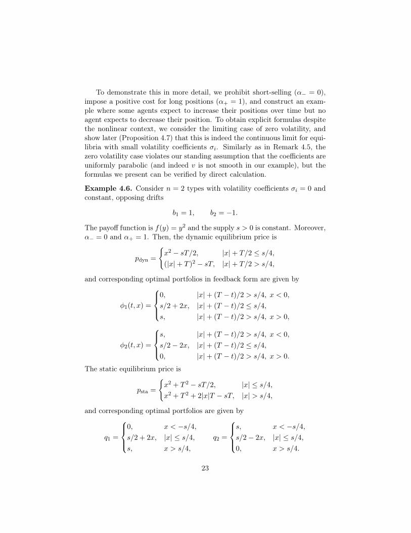
To demonstrate this in more detail, we prohibit short-selling (α− = 0),impose a positive cost for long positions (α+ = 1), and construct an exam-ple where some agents expect to increase their positions over time but noagent expects to decrease their position. To obtain explicit formulas despitethe nonlinear context, we consider the limiting case of zero volatility, andshow later (Proposition 4.7) that this is indeed the continuous limit for equi-libria with small volatility coefficients σi. Similarly as in Remark 4.5, thezero volatility case violates our standing assumption that the coefficients areuniformly parabolic (and indeed v is not smooth in our example), but theformulas we present can be verified by direct calculation.

Example 4.6. Consider n = 2 types with volatility coefficients σi = 0 andconstant, opposing drifts

b1 = 1, b2 = −1.

The payoff function is f(y) = y2 and the supply s > 0 is constant. Moreover,α− = 0 and α+ = 1. Then, the dynamic equilibrium price is

pdyn =

x2 − sT/2, |x|+ T/2 ≤ s/4,(|x|+ T )2 − sT, |x|+ T/2 > s/4,

and corresponding optimal portfolios in feedback form are given by

φ1(t, x) =

0, |x|+ (T − t)/2 > s/4, x < 0,

s/2 + 2x, |x|+ (T − t)/2 ≤ s/4,s, |x|+ (T − t)/2 > s/4, x > 0,

φ2(t, x) =

s, |x|+ (T − t)/2 > s/4, x < 0,

s/2− 2x, |x|+ (T − t)/2 ≤ s/4,0, |x|+ (T − t)/2 > s/4, x > 0.

The static equilibrium price is

psta =

x2 + T 2 − sT/2, |x| ≤ s/4,x2 + T 2 + 2|x|T − sT, |x| > s/4,

and corresponding optimal portfolios are given by

q1 =

0, x < −s/4,s/2 + 2x, |x| ≤ s/4,s, x > s/4,

q2 =

s, x < −s/4,s/2− 2x, |x| ≤ s/4,0, x > s/4.

23

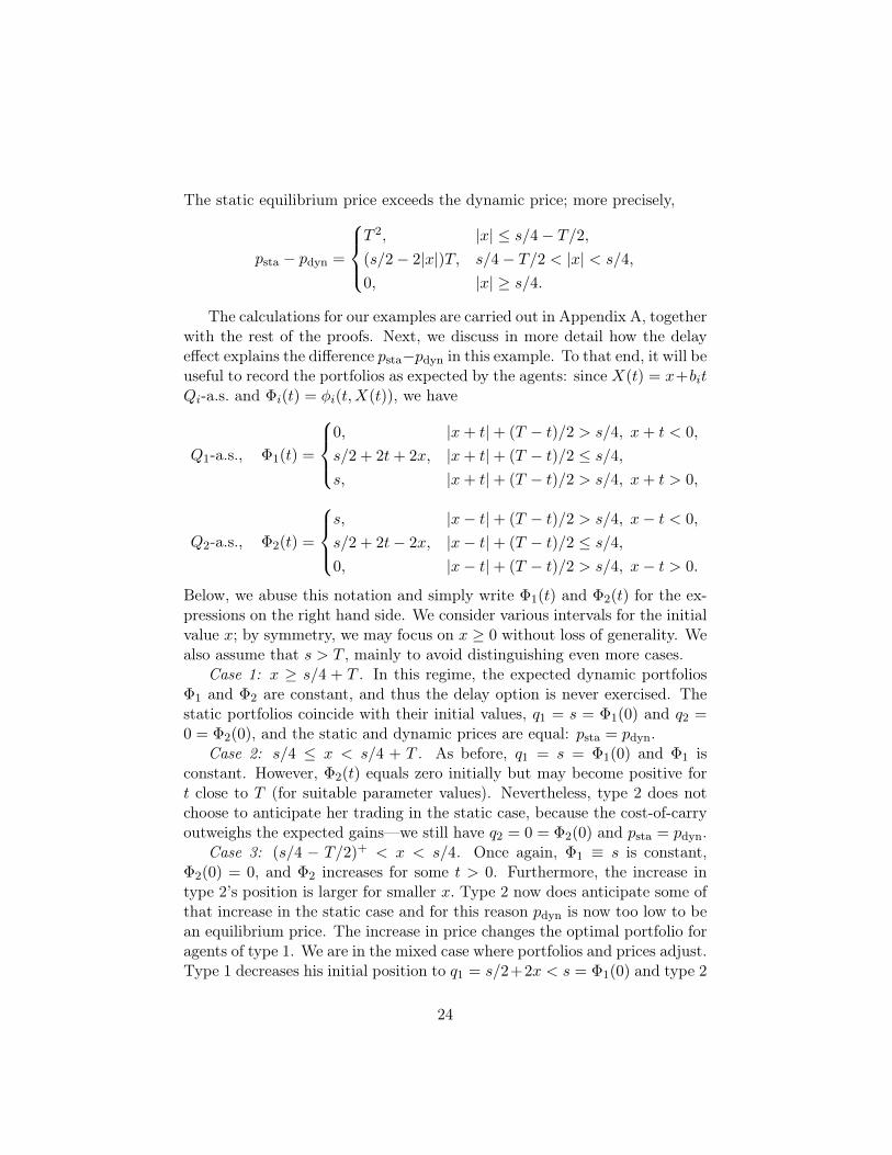
The static equilibrium price exceeds the dynamic price; more precisely,

psta − pdyn =

T 2, |x| ≤ s/4− T/2,(s/2− 2|x|)T, s/4− T/2 < |x| < s/4,

0, |x| ≥ s/4.

The calculations for our examples are carried out in Appendix A, togetherwith the rest of the proofs. Next, we discuss in more detail how the delayeffect explains the difference psta−pdyn in this example. To that end, it will beuseful to record the portfolios as expected by the agents: since X(t) = x+bitQi-a.s. and Φi(t) = φi(t,X(t)), we have

Q1-a.s., Φ1(t) =

0, |x+ t|+ (T − t)/2 > s/4, x+ t < 0,

s/2 + 2t+ 2x, |x+ t|+ (T − t)/2 ≤ s/4,s, |x+ t|+ (T − t)/2 > s/4, x+ t > 0,

Q2-a.s., Φ2(t) =

s, |x− t|+ (T − t)/2 > s/4, x− t < 0,

s/2 + 2t− 2x, |x− t|+ (T − t)/2 ≤ s/4,0, |x− t|+ (T − t)/2 > s/4, x− t > 0.

Below, we abuse this notation and simply write Φ1(t) and Φ2(t) for the ex-pressions on the right hand side. We consider various intervals for the initialvalue x; by symmetry, we may focus on x ≥ 0 without loss of generality. Wealso assume that s > T , mainly to avoid distinguishing even more cases.

Case 1: x ≥ s/4 + T . In this regime, the expected dynamic portfoliosΦ1 and Φ2 are constant, and thus the delay option is never exercised. Thestatic portfolios coincide with their initial values, q1 = s = Φ1(0) and q2 =0 = Φ2(0), and the static and dynamic prices are equal: psta = pdyn.

Case 2: s/4 ≤ x < s/4 + T . As before, q1 = s = Φ1(0) and Φ1 isconstant. However, Φ2(t) equals zero initially but may become positive fort close to T (for suitable parameter values). Nevertheless, type 2 does notchoose to anticipate her trading in the static case, because the cost-of-carryoutweighs the expected gains—we still have q2 = 0 = Φ2(0) and psta = pdyn.

Case 3: (s/4 − T/2)+ < x < s/4. Once again, Φ1 ≡ s is constant,Φ2(0) = 0, and Φ2 increases for some t > 0. Furthermore, the increase intype 2’s position is larger for smaller x. Type 2 now does anticipate some ofthat increase in the static case and for this reason pdyn is now too low to bean equilibrium price. The increase in price changes the optimal portfolio foragents of type 1. We are in the mixed case where portfolios and prices adjust.Type 1 decreases his initial position to q1 = s/2+2x < s = Φ1(0) and type 2

24

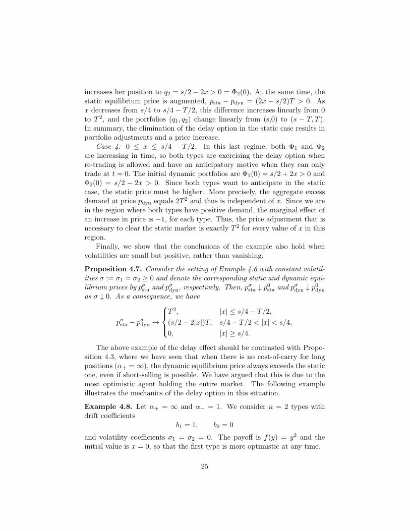
increases her position to q2 = s/2− 2x > 0 = Φ2(0). At the same time, thestatic equilibrium price is augmented, psta − pdyn = (2x − s/2)T > 0. Asx decreases from s/4 to s/4 − T/2, this difference increases linearly from 0to T 2, and the portfolios (q1, q2) change linearly from (s,0) to (s − T, T ).In summary, the elimination of the delay option in the static case results inportfolio adjustments and a price increase.

Case 4: 0 ≤ x ≤ s/4 − T/2. In this last regime, both Φ1 and Φ2

are increasing in time, so both types are exercising the delay option whenre-trading is allowed and have an anticipatory motive when they can onlytrade at t = 0. The initial dynamic portfolios are Φ1(0) = s/2 + 2x > 0 andΦ2(0) = s/2 − 2x > 0. Since both types want to anticipate in the staticcase, the static price must be higher. More precisely, the aggregate excessdemand at price pdyn equals 2T 2 and thus is independent of x. Since we arein the region where both types have positive demand, the marginal effect ofan increase in price is −1, for each type. Thus, the price adjustment that isnecessary to clear the static market is exactly T 2 for every value of x in thisregion.

Finally, we show that the conclusions of the example also hold whenvolatilities are small but positive, rather than vanishing.

Proposition 4.7. Consider the setting of Example 4.6 with constant volatil-ities σ := σ1 = σ2 ≥ 0 and denote the corresponding static and dynamic equi-librium prices by pσsta and pσdyn, respectively. Then, p

σsta ↓ p0

sta and pσdyn ↓ p0dyn

as σ ↓ 0. As a consequence, we have

pσsta − pσdyn →

T 2, |x| ≤ s/4− T/2,(s/2− 2|x|)T, s/4− T/2 < |x| < s/4,

0, |x| ≥ s/4.

The above example of the delay effect should be contrasted with Propo-sition 4.3, where we have seen that when there is no cost-of-carry for longpositions (α+ =∞), the dynamic equilibrium price always exceeds the staticone, even if short-selling is possible. We have argued that this is due to themost optimistic agent holding the entire market. The following exampleillustrates the mechanics of the delay option in this situation.

Example 4.8. Let α+ = ∞ and α− = 1. We consider n = 2 types withdrift coefficients

b1 = 1, b2 = 0

and volatility coefficients σ1 = σ2 = 0. The payoff is f(y) = y2 and theinitial value is x = 0, so that the first type is more optimistic at any time.

25

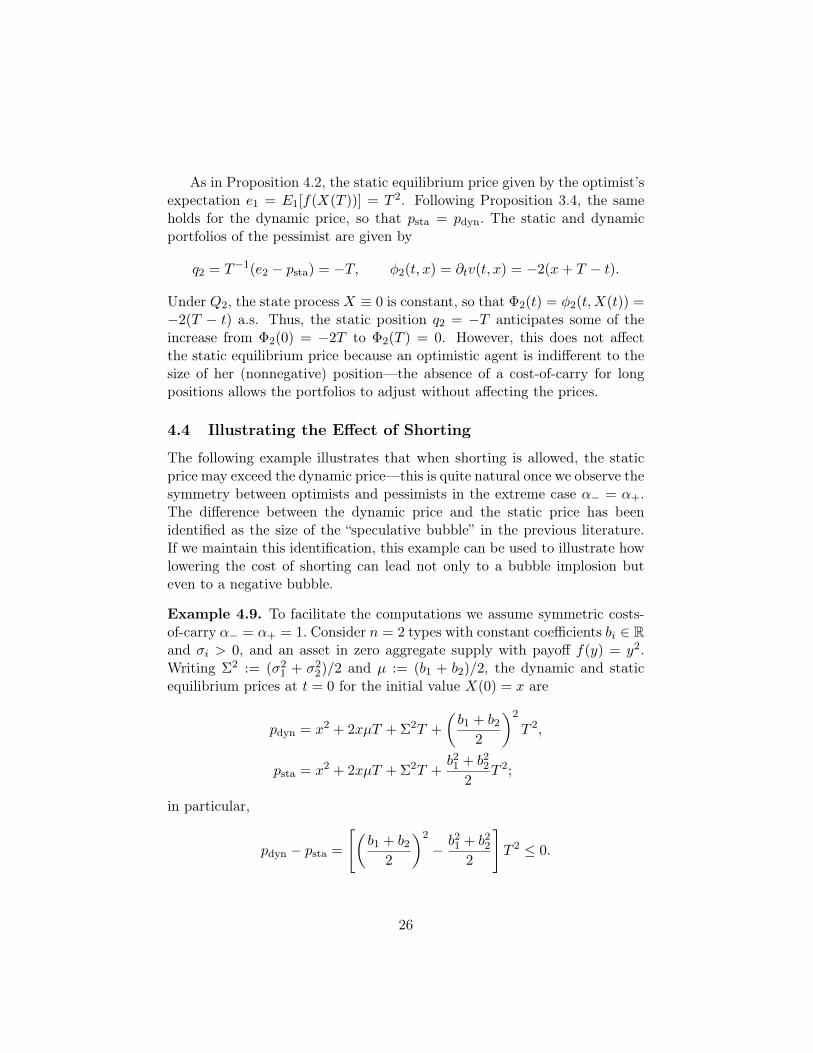
As in Proposition 4.2, the static equilibrium price given by the optimist’sexpectation e1 = E1[f(X(T ))] = T 2. Following Proposition 3.4, the sameholds for the dynamic price, so that psta = pdyn. The static and dynamicportfolios of the pessimist are given by

q2 = T−1(e2 − psta) = −T, φ2(t, x) = ∂tv(t, x) = −2(x+ T − t).

Under Q2, the state process X ≡ 0 is constant, so that Φ2(t) = φ2(t,X(t)) =−2(T − t) a.s. Thus, the static position q2 = −T anticipates some of theincrease from Φ2(0) = −2T to Φ2(T ) = 0. However, this does not affectthe static equilibrium price because an optimistic agent is indifferent to thesize of her (nonnegative) position—the absence of a cost-of-carry for longpositions allows the portfolios to adjust without affecting the prices.

4.4 Illustrating the Effect of Shorting

The following example illustrates that when shorting is allowed, the staticprice may exceed the dynamic price—this is quite natural once we observe thesymmetry between optimists and pessimists in the extreme case α− = α+.The difference between the dynamic price and the static price has beenidentified as the size of the “speculative bubble” in the previous literature.If we maintain this identification, this example can be used to illustrate howlowering the cost of shorting can lead not only to a bubble implosion buteven to a negative bubble.

Example 4.9. To facilitate the computations we assume symmetric costs-of-carry α− = α+ = 1. Consider n = 2 types with constant coefficients bi ∈ Rand σi > 0, and an asset in zero aggregate supply with payoff f(y) = y2.Writing Σ2 := (σ2

1 + σ22)/2 and µ := (b1 + b2)/2, the dynamic and static

equilibrium prices at t = 0 for the initial value X(0) = x are

pdyn = x2 + 2xµT + Σ2T +

(b1 + b2

2

)2

T 2,

psta = x2 + 2xµT + Σ2T +b21 + b22

2T 2;

in particular,

pdyn − psta =

[(b1 + b2

2

)2

− b21 + b222

]T 2 ≤ 0.

26

The optimal dynamic and static portfolios are given by

φi(t, x) = x(bi − bj) + 12(T − t)(b2i − b2j ) + 1

2(σ2i − σ2

j ),

qi = x(bi − bj) + 12T (b2i − b2j ) + 1

2(σ2i − σ2

j ),

where j = 2 if i = 1 and vice versa; in particular, the demands at t = 0coincide. In the special case b1 = b2 where all agents agree on the drift, wehave pdyn = psta and the demands coincide at all times. Whenever b1 6= b2, acontinuity result similar to the results established in Section 3.2 guaranteesthat pdyn < psta for cost parameters close to α− = α+ = 1.

To obtain some intuition for this example, consider the case were σ1 = σ2,b1 > 0 and b2 = 0. Then if x > 0, type 1 is long and type 2 is shortwhen re-trading is allowed. Notice that an agent who is short expects onaverage to cover some of her shorts in the future. When re-trading is ruledout, she prefers to cut her short position at time zero. This would placeupward pressure on the static price. The long party also expects to reducehis position if x would stay constant, but because b1 > 0, he expects thestate X(t) to grow, thus dampening his need to anticipate the reductionwhen re-trading is ruled out. In other words, the long party values the resaleoption less than the short party values the repurchase option. As a result,the static market presents excess demand at price pdyn and thus the staticprice must rise to clear the market.

5 Conclusion

In this paper, we considered a continuous-time model of trading among risk-neutral agents with heterogeneous beliefs. Agents face quadratic costs-of-carry and as a consequence, their marginal valuation of the asset decreaseswhen the magnitude of their position increases, as it would be the casefor risk-averse agents. In previous models of heterogeneous beliefs, it wasassumed that agents face a constant marginal cost-of-carry for a positiveposition and an infinite cost for a negative position. As a result, buyersbenefit from a resale option and are willing to pay for an asset in excessof their own valuation of the dividends of that asset. Moreover, the supplydoes not affect the equilibrium price. We show that when buyers face anincreasing marginal cost-of-carry, in equilibrium, they may also value anoption to delay. We illustrate with an example that even when shorting isimpossible, this delay option may cause the market to equilibrate below theprice that would prevail if agents were restricted to buy-and-hold strategies.

27

Moreover, we introduce the possibility of short-selling and show how thisgives pessimists the analogous options. In our model, the price dependson the supply. We characterize the unique equilibrium of our model asthe solution to a Hamilton–Jacobi–Bellman of a novel form and use this toderive several comparative statics: the price decreases with an increase in thesupply of the asset, with an increase in the cost of carrying long positions,and with a decrease in the cost of carrying short positions. The conclusionsof earlier models are shown to hold in a limiting case of the model when thecost-of-carry for long positions tends to zero.

In our model the demand for the asset is satisfied by the sum of twocomponents—the exogenous supply and the short positions of the marketparticipants. While the shorts are determined endogenously, the supply isindependent of the current price and the beliefs of agents. It would be inter-esting to model this supply as originating from parties solving an appropriateoptimization problem.

A Proofs

This appendix collects the proofs for the results in Sections 2–4.

A.1 Proofs for Section 2

Before proving the main result of Theorem 2.1, we record two lemmas forlater reference. The first one guarantees the passage from almost-sure topointwise identities.

Lemma A.1. For all i ∈ 1, . . . , n and all t ∈ (0, T ], the support of X(t)under Qi is the full space Rd.

Proof. Since bi is bounded and σ2i is uniformly parabolic, the support of Qi

in Ω is the set of all paths ω ∈ C([0, T ],Rd) with ω(0) = x; see (Stroock andVaradhan, 1972, Theorem 3.1). The claim is a direct consequence.

The second lemma provides an expression for the optimal portfolios.

Lemma A.2. Let v ∈ C1,2b and consider the (price) process P (t) = v(t,X(t)).

The portfolio defined by Φi(t) = φi(t,X(t)), where

φi(t, x) = αsign(Liv(t,x))Liv(t, x), (A.1)

is the unique26 optimal portfolio for type i.26We recall that uniqueness is understood up to (Qi × dt)-nullsets.

28

Proof. We note that Φi is admissible since v ∈ C1,2b . Let Φ be any admissible

portfolio. By Itô’s formula,∫ T

0Φ(t) dP (t)−

∫ T

0c(Φ(t)) dt =

∫ T

0Φ(t)Liv(t,X(t))−c(Φ(t)) dt+Mi(T )

where Mi(T ) is the terminal value of a (true) martingale with vanishingexpectation; recall that σi and ∂xv are bounded. Thus, the expected finalpayoff (2.3) is given by

Ei

[∫ T

0Φ(t)Liv(t,X(t))− c(Φ(t)) dt

].

As a result, Φ is optimal if and only if it maximizes the above integrand (upto (Qi × dt)-nullsets). The unique maximizer is given by Φi, and the claimfollows.

We can now prove the main result on the pricing PDE.

Proof of Theorem 2.1. (a) We first show that a given equilibrium price func-tion v ∈ C1,2

b solves the PDE. Since v(T,X(T )) = f(X(T )) Qi-a.s. for all i,the terminal condition v(T, ·) = f follows from Lemma A.1. At any state(t, x), we introduce the set

I∗(t, x) = i ∈ 1, . . . , n : Liv(t, x) < 0. (A.2)

Next, we recall the unique optimal portfolios Φi from Lemma A.2. Usingagain Lemma A.1, the market clearing condition

∑i Φi = S can be stated

asα−∑i∈I∗

Liv + α+

∑i∈Ic∗

Liv = s. (A.3)

If i ∈ I∗, then Liv ≤ 0 and α− ≤ α+ implies α−Liv ≥ α+Liv. Conversely, ifi ∈ Ic∗, then Liv ≥ 0 and α+Liv ≥ α−Liv. It follows that the set I∗ of (A.2)maximizes the left hand side of (A.3) among all subsets I ⊆ 1, . . . , n. Thatis,

maxI⊆1,...,n

(α−∑i∈ILiv + α+

∑i∈IcLiv − s

)= 0 (A.4)

and the set I∗ is a maximizer, or equivalently,

maxI⊆1,...,n

1|I|α−+|Ic|α+

(α−∑i∈ILiv + α+

∑i∈IcLiv − s

)= 0. (A.5)

29

After plugging in the definition of Liv and using the definitions of µI , ΣI

and κI in (2.6)–(2.8), this is the desired PDE (2.5).

(b) Conversely, let v ∈ C1,2b be a solution of the PDE (2.5) with termi-

nal condition f and define Φi, φi as in part (i) of Theorem 2.1. Then, theterminal condition v(T,X(T )) = f(X(T )) is satisfied and Φi are optimalby Lemma A.2. Since v is a solution of the equivalent PDE (A.4) and I∗of (A.2) is a maximizer, we have that∑

1≤i≤nφi = α−

∑i∈I∗

Liv + α+

∑i∈Ic∗

Liv = s;

that is, the market clears. This shows that v is an equilibrium price function.

(c) Since (a) and (b) established a one-to-one correspondence betweenequilibria and solutions of the PDE (2.5) with terminal condition f , it re-mains to observe that the latter has a unique solution in C1,2

b . Indeed,existence holds by (Krylov, 1987, Theorem 6.4.3, p. 301); the conditions inthe cited theorem can be verified as in (Krylov, 1987, Example 6.1.4, p. 279).Uniqueness holds by the comparison principle for parabolic PDEs; see (Flem-ing and Soner, 2006, Theorem V.9.1, p. 223).

Next, we prove the optimal control representation for the equilibriumprice function.

Proof of Proposition 2.4. By Theorem 2.1, the function v ∈ C1,2b is a solution

of the PDE (2.5) which is the Hamilton–Jacobi–Bellman equation of thecontrol problem (2.10). Moreover, I∗(t, x) maximizes the Hamiltonian asnoted after (A.4). Thus, the verification theorem of stochastic control, cf.(Fleming and Soner, 2006, Theorem IV.3.1, p. 157), shows that v is the valuefunction and I∗ is an optimal control.

It remains to analyze the planner’s problem.

Proof of Theorem 2.5. (i) In what follows, we fix the assignment I(t) =I(t,X(t)) and often omit the dependence on I in the notation. Suppose thatw is an equilibrium price function; we show that w satisfies (2.12). As inLemma A.2, the unique optimal portfolio for agent i is given by Φi(t) = φi(t),where

φi(t, x) = αi(t, x)Liw(t, x). (A.6)

The market clearing condition then implies

α−∑i∈ILiw + α+

∑i∈IcLiw = s,

30

which is equivalent to

1|I|α−+|Ic|α+

(α−∑i∈ILiw + α+

∑i∈IcLiw − s

)= 0

or∂tw + µI∂xw + 1

2 Tr Σ2I∂xxw − κI = 0.

Given the terminal condition f , this linear PDE has a unique solution inC1,2b which, by the Feynman–Kac formula (Karatzas and Shreve, 1991, The-

orem 5.7.6, p. 366), has the representation (2.12).Conversely, starting with the unique solution w = vI ∈ C1,2

b of that PDE,reversing the above arguments shows that w is an equilibrium price function,and that completes the proof of (i).

(ii) In view of (2.12), (2.10) and Proposition 2.4, the supremum of vI(t, x)over all assignments I(t) = I(t,X(t)) is given by V (t, x) and (2.11) is anoptimal assignment in feedback form.

A.2 Proofs for Section 3

We start with the comparative statics for the dependence of the price on thesupply.

Proof of Proposition 3.1. Since the function s enters linearly in the runningcost (2.8) of the control problem (2.10) and nowhere else, it follows imme-diately that the value function V is monotone decreasing in s, and now theclaim follows from Proposition 2.4.

Next, we consider the dependence on the cost coefficients.

Proof of Proposition 3.2 and Remark 3.3. Let α− ≤ α+ and α′− ≤ α′+ betwo pairs of cost coefficients and let v and v′ be the corresponding equilibriumprice functions. Let I∗ be the optimal feedback control for α± as definedin (A.2), then by (A.4) we have

α−∑i∈I∗

Liv + α+

∑i∈Ic∗

Liv − s = 0.

If α′− ≤ α− and α′+ ≥ α+, then∑

i∈I∗ Liv ≤ 0 and

∑i∈Ic∗ L

iv ≥ 0 yield that

α′−∑i∈I∗

Liv + α′+∑i∈Ic∗

Liv − s ≥ 0.

31

In the special case where s ≡ 0, this conclusion also holds under the weakercondition that α+/α− ≤ α′+/α

′−, which covers the case (iii), and the same

holds under the conditions of Remark 3.3. It then follows that

maxI⊆1,...,n

(α′−∑i∈ILiv + α′+

∑i∈IcLiv − s

)≥ 0,

which is a version of (A.4) with inequality instead of equality, for the coeffi-cients α′±. Following the same steps as after (A.4), we deduce that

∂tv + supI⊆1,...,n

(µ′I∂xv + 1

2 Tr Σ′2I ∂xxv − κ′I

)≥ 0,

where µ′I ,Σ′I , κ′I are defined as in (2.6)–(2.8) but with α′± instead of α±.

In other words, v is a subsolution27 of the PDE satisfied by v′. As v andv′ satisfy the same terminal condition f , the comparison principle (Flemingand Soner, 2006, Theorem V.9.1, p. 223) implies that v ≤ v′.

We continue with our result on the limit α+ →∞.

Proof of Proposition 3.4. We first notice that since s ≥ 0, the optimal set I∗of (A.2) for the Hamiltonian of the PDE (2.5) must satisfy |I∗| < n due tothe market clearing condition—at least one agent has to hold a nonnegativeposition. As a result, the PDE (2.5) remains the same if the supremum istaken only over sets I with |Ic| > 0.

Taking that into account, the limiting PDE for (2.5) as α+ →∞ is

∂tv + sup∅6=J⊆1,...,n

1|J |

∑i∈J

(bi∂xv + 1

2 Trσ2i ∂xxv

)= 0. (A.7)

Notice that given a set of real numbers, the largest average over a subset isin fact equal to the largest number in the set. As a result, (A.7) coincideswith (3.1). Using again (Krylov, 1987, Theorem 6.4.3, p. 301) and (Flemingand Soner, 2006, Theorem V.9.1, p. 223), this equation has a unique solutionv∞ ∈ C1,2

b for the terminal condition f , and the solution is independent ofα− and s since these quantities do not appear in (3.1).

To see that vα−,α+(t, x) → v∞(t, x), one can apply a PDE techniquecalled the Barles–Perthame procedure to the equations under consideration;see (Fleming and Soner, 2006, Section VII.3). Alternately, and to give a

27Note that the sign convention chosen here is opposite to the one of Fleming and Soner(2006), so that a subsolution corresponds to the inequality ≥ 0 in the PDE.

32

more concise proof, we may use the representation (2.10) of vα−,α+ as avalue function as well as the corresponding representation for v∞. Then, aresult on the stability of value functions, cf. (Krylov, 1980, Corollary 3.1.13,p. 138), shows that vα−,α+ → v∞ locally uniformly; that is,

sup(t,x)∈[0,T ]×K

|vα−,α+(t, x)− v∞(t, x)| → 0

for any compact set K ⊆ Rd. The monotonicity property of the limit followsfrom Proposition 3.2.

Finally, we turn to the limit α− → 0.

Proof of Proposition 3.6. The arguments are similar to the ones for Propo-sition 3.4. In this case, the limiting PDE for (2.5) as α− → 0 is (3.3). Asin the proof of Proposition 3.4 we have that the limiting PDE has a uniquesolution v0,α+ ∈ C1,2

b and vα−,α+(t, x) → v0,α+(t, x) locally uniformly, withmonotonicity in α−. In the special case where s = 0, the PDE (3.3) coincideswith (A.7), and thus with (3.1) as shown in the proof of Proposition 3.4.

A.3 Proofs for Section 4

We first prove our formula for the static equilibrium price.

Proof of Proposition 4.1. We set ei = Ei[f(X(T ))]. Given any price p, theexpected net payoff for agent i using portfolio q is

q(ei − p)− T2αsign(q)

q2

and the unique maximizer is qi = αsign(ei−p)T−1(ei − p) as stated in (4.2).

Let p be a static equilibrium price. Setting I∗ = i ∈ 1, . . . , n : ei < p,the market clearing condition

∑i qi = s for these optimal portfolios yields

α−∑i∈I∗

(ei − p) + α+

∑i∈Ic∗

(ei − p) = sT (A.8)

and we observe that I∗ maximizes the left hand side; that is,

maxI⊆1,...,n

(α−∑i∈I

(ei − p) + α+

∑i∈Ic

(ei − p)− sT

)= 0.

This is equivalent to the claimed representation (4.1) for p.

33

Conversely, define p by (4.1) and qi by (4.2), then qi is optimal for agent ias mentioned in the beginning of the proof. Moreover, reversing the above,p satisfies (A.8) and thus

n∑i=1

qi = α−∑i∈I∗

T−1(ei − p) + α+

∑i∈Ic∗

T−1(ei − p) = s,

establishing market clearing.

We can now deduce the formulas for the limiting cases of the static equi-librium.

Proof of Proposition 4.2. Formula (4.3) follows by taking the limit α+ →∞in (4.1). Similarly, (4.4) is obtained by taking the limit α− → 0 in (4.1).

Next, we show that in the limit α+ →∞ with no cost on long positions,the dynamic price exceeds the static one.

Proof of Proposition 4.3. By the formula (4.3) for p∞sta, it suffices to verifythat Ei[f(X(T ))] ≤ p∞dyn for fixed i ∈ 1, . . . , n. Indeed, let u = ui ∈ C1,2

b

be the unique solution of

∂tu+ bi∂xu+ 12 Trσ2

i ∂xxu = 0, u(T, ·) = f.

Then, by the Feynman–Kac formula (Karatzas and Shreve, 1991, Theo-rem 5.7.6, p. 366), we have u(0, x) = Ei[f(X(T ))]. Moreover, u is clearlya subsolution of the PDE (3.1) for v∞, and now the comparison principle(Fleming and Soner, 2006, Theorem V.9.1, p. 223) yields that Ei[f(X(T ))] =u(0, x) ≤ v∞(0, x) = p∞dyn as claimed.

In what follows, we show that in the limit α− → 0 where short-selling isprohibited, the same inequality holds, provided one agents holds the staticmarket.

Proof of Proposition 4.4. In view of (4.4), we have p0,α+sta = Ei[f(X(T ))]− sT

α+

since the maximizing set is J = i. Using again the Feynman–Kac formula(Karatzas and Shreve, 1991, Theorem 5.7.6, p. 366), we deduce that p0,α+

sta =u(0, x) where u ∈ C1,2

b is the solution of

∂tu+ bi∂xu+ 12 Trσ2

i ∂xxu−sT

α+= 0, u(T, ·) = f.

In particular, u is a subsolution of the PDE (3.3) for v0,α+ , and now the com-parison principle (Fleming and Soner, 2006, Theorem V.9.1, p. 223) yieldsthat p0,α+

sta = u(0, x) ≤ v0,α+(0, x) = p0,α+

dyn as desired.

34

We turn to our example where the static price exceeds the dynamic onedue to the delay effect.

Proofs for Example 4.6. We begin with the static case. For later use, weconsider the more general situation where σ := σ1 = σ2 may be positive(but constant). We have ei = Ei[f(X(T ))] = x2 + 2xbiT + T 2 + σ2T andthus, as in (4.4), the static price psta is

psta = max∅6=J⊆1,2

(1|J |

∑i∈J

ei −sT

|J |

)= x2 + σ2T + max

T 2 − sT/2, T 2 + 2|x|T − sT

or

psta =

x2 + σ2T + T 2 − sT/2, |x| ≤ s/4,x2 + σ2T + T 2 + 2|x|T − sT, |x| > s/4

(A.9)

and the portfolios qi are as stated in Example 4.6.We turn to the dynamic case and restrict to σ = 0. The limiting equation

for (3.3) is

∂tv + max (|∂xv| − s,−s/2) = 0, v(T, ·) = f. (A.10)

In analogy to Proposition 2.4, this can be seen as the Hamilton–Jacobi equa-tion of a deterministic control problem where the drift µ of the controlledstate dX(t) = µ(t,X(t)) dt can be chosen to be ±1 or 0 and the running costis s or s/2, respectively. We can check directly that an optimal control forthis problem is

µ(t, x) =

sign(x), |x|+ (T − t)/2 > s/4,

0, |x|+ (T − t)/2 ≤ s/4,

and then the value function is found to be

v(t, x) =

(|x|+ T − t)2 − s(T − t), |x|+ (T − t)/2 > s/4,

x2 − s(T − t)/2, |x|+ (T − t)/2 ≤ s/4.

Indeed, v is continuous and the unique viscosity28 solution of (A.10). Theindicated formulas for pdyn−psta = v(0, x)−psta and for the optimal controlsφi follow.

28 As is often the case for deterministic control problems, the value function is not C1,1

and (A.10) has no classical solution.

35

Next, we prove the continuity of the prices in the small volatility limit.

Proof of Proposition 4.7. For the static case, the formula for pσsta statedin (A.9) shows that pσsta − p0

sta = σ2T ↓ 0. Turning to the dynamic case,we first show that pσdyn = vσ(0, x) is monotone with respect to σ. Since f isconvex, x 7→ vσ(t, x) is convex and thus ∂xxvσ ≥ 0. Given σ1 ≥ σ2 > 0, itfollows that vσ2 is a subsolution to the equation (3.3) for vσ1 , and thus thecomparison principle for parabolic PDEs implies that vσ1 ≥ vσ2 . To see thatvσ(t, x)→ v0(t, x) and in particular pσdyn → p0

dyn, we may again use a generalresult on the stability of value functions; cf. (Krylov, 1980, Corollary 3.1.13,p. 138).

It remains to provide the calculations for our symmetric example withα− = α+ = 1.

Proofs for Example 4.9. Following Remark 3.5, the equilibrium price func-tion in the dynamic case is

v(t, x) = E[f(x+ µτ + ΣBτ )], where τ := T − t

and Bτ is a centered Gaussian with variance τ . As f(y) = y2,

v(t, x) = x2 + 2xµτ + µ2τ2 + Σ2τ

and the optimal portfolios in feedback form are given by

φi(t, x) = Liv(t, x) = x(bi − bj) + 12τ(b2i − b2j ) + 1

2(σ2i − σ2

j ).

For the static case, we have

ei = x2 + 2xbiT + b2iT2 + σ2

i T

and thus

psta =e1 + e2

2= x2 + 2xµT +

b21 + b222

T 2 + Σ2T

as well as

qi = T−1(ei − psta) = T−1 ei − ej2

= x(bi − bj) + 12T (b2i − b2j ) + 1

2(σ2i − σ2

j ).

36

B Adding Linear Costs

In this section, we generalize the cost-of-carry by adding linear terms anddiscuss the corresponding changes in our main results. Broadly speaking,the generalized model does not alter the economic conclusions.

Indeed, let

c(y) =

1

2α+y2 + β+y, y ≥ 0,

12α−

y2 + β−|y|, y < 0,(B.1)

where β−, β+ ≥ 0 are constants; as discussed in the Introduction, the maincase of interest is β− > 0 and β+ = 0. While this cost function is still strictlyconvex, it fails to be differentiable at y = 0 unless β− = β+ = 0.

Following the proof of Lemma A.2, the optimal portfolio (A.1) then be-comes

φi(t, x) =

α+(Liv(t, x)− β+), Liv(t, x) ≥ β+,

α−(Liv(t, x) + β−), Liv(t, x) ≤ −β−,0, else.

(B.2)

That is, there is an interval [−β−, β+] of values of Liv(t, x) where it is optimalto have a zero position, due to the kink in the function c.

The main PDE (2.5) needs to be adapted correspondingly. Indeed, in-stead of considering only the group I of agents holding a short position, wenow need to distinguish a group J of agents holding a (strict) long position—the group J may be smaller than the complement Ic. More precisely, thegeneralized PDE (2.5) reads as follows (the proof is analogous to Theo-rem 2.1).

Theorem B.1. The unique equilibrium price function v ∈ C1,2b can be char-

acterized as the unique solution of the PDE

∂tv(t, x)+ supI∩J=∅

(µI,J(t, x)∂xv(t, x)+1

2 Tr Σ2I,J(t, x)∂xxv(t, x)−κI,J(t, x)

)= 0

(B.3)on [0, T )× Rd with terminal condition v(T, x) = f(x), where the supremumis taken over all disjoint subsets I, J ⊆ 1, . . . , n and the coefficients aredefined as

µI,J(t, x) = α−|I|α−+|J |α+

∑i∈I

bi(t, x) + α+

|I|α−+|J |α+

∑i∈J

bi(t, x),

Σ2I,J(t, x) = α−

|I|α−+|J |α+

∑i∈I

σ2i (t, x) + α+

|I|α−+|J |α+

∑i∈J

σ2i (t, x),

37

κI,J(t, x) =s(t, x)− |I|α−β− + |J |α+β+

|I|α− + |J |α+.

In particular, the additional constants β−, β+ enter only through therunning cost κI,J . It follows that the results on the comparative staticsin Propositions 3.1 and 3.2 remain valid; in addition, the equilibrium pricefunction v is increasing with respect to β− and decreasing with respect to β+.

In the limiting case of zero cost for long positions, we now need to sendα+ →∞ and β+ → 0. Then, the result of Proposition 3.4 is unchanged; i.e.,the limiting equilibrium price function is the solution of

∂tv + supi∈1,...,n

(bi∂xv + 1

2 Trσ2i ∂xxv

)= 0.

On the other hand, for the limit α− → 0 of infinite cost for shorting, the re-sult of Proposition 3.6 changes slightly because the long positions are subjectto β+ which becomes an additional running cost in the limiting equation

∂tv + sup∅6=J⊆1,...,n

(1|J |

∑i∈J

bi∂xv + 12 Tr 1

|J |

∑i∈J

σ2i ∂xxv −

s

|J |α+− β+

)= 0.

The results for the static equilibrium problem can be generalized with anal-ogous changes.

C Heterogeneous Costs

In this section, we show how the equilibrium of Theorem 2.1 changes if thecost coefficients α−, α+ depend on the type rather than being the same for allagents. We write αi−, αi+ for the coefficients of type i. The following resultshows that while the structure of the equilibrium remains similar, agentswith lower costs have a larger influence on the coefficients of the PDE thatdetermines the equilibrium price.

Theorem C.1. The unique equilibrium price function v ∈ C1,2b can be char-

acterized as the unique solution of the PDE (2.5) with coefficients

µI(t, x) =1∑

i∈I αi− +

∑i∈Ic α

i+

(∑i∈I

αi−bi(t, x) +∑i∈Ic

αi+bi(t, x)

),

Σ2I(t, x) =

1∑i∈I α

i− +

∑i∈Ic α

i+

(∑i∈I

αi−σ2i (t, x) +

∑i∈Ic

αi+σ2i (t, x)

),

κI(t, x) =s(t, x)∑

i∈I αi− +

∑i∈Ic α

i+

.

38

The proof is analogous to Theorem 2.1. As in Lemma A.2, the optimalportfolios are given by αi±Liv(t, x). Thus, as expected, types with lowercosts hold larger positions.

References

Beltran, D. O., L. Cordell, and C. P. Thomas. 2017. Asymmetric informationand the death of ABS CDOs. Journal of Banking & Finance 76:1–14.

Berestycki, H., C. Bruggeman, R. Monneau, and J. A. Scheinkman.2016. Bubbles in assets with finite life. Available at SSRN:https://ssrn.com/abstract=2617078 .

Carlos, A., L. Neal, and K. Wandschneider. 2006. Dissecting the anatomy ofexchange alley: The dealings of stockjobbers during and after the SouthSea bubble. Unpublished paper, University of Illinois .

Cochrane, J. H. 2002. Stocks as money: Convenience yield and the tech-stockbubble. Tech. rep., National Bureau of Economic Research.

Cordell, L., Y. Huang, and M. Williams. 2011. Collateral damage: Sizingand assessing the subprime CDO crisis. Working Paper 11-30/R, ResearchDepartment Federal Reserve Bank of Philadelphia.

D’Avolio, G. 2002. The market for borrowing stock. Journal of FinancialEconomics 66 (2-3):271–306.

Diether, K. B., C. J. Malloy, and A. Scherbina. 2002. Differences of opinionand the cross section of stock returns. Journal of Finance 57 (5):2113–2141.

Duffie, D., N. Gârleanu, and L. H. Pedersen. 2005. Over-the-counter markets.Econometrica 73 (6):1815–1847.

Dumas, B., A. Kurshev, and R. Uppal. 2009. Equilibrium portfolio strategiesin the presence of sentiment risk and excess volatility. Journal of Finance64 (2):579–629.

Feldhütter, P. 2012. The same bond at different prices: Identifying searchfrictions and selling pressures. Review of Financial Studies 25 (4):1155–1206.

39

Fleming, W. H. and H. M. Soner. 2006. Controlled Markov Processes andViscosity Solutions. Springer, New York, 2nd ed.

Foote, C. L., K. S. Gerardi, and P. S. Willen. 2012. Why Did So Many PeopleMake So Many Ex Post Bad Decisions? The Causes of the ForeclosureCrisis. In Rethinking the Financial Crisis, edited by A. Blinder, A. Lo,and R. Solow, 136–186. Russell Sage Foundation.

Harris, R. 1994. The Bubble Act: Its passage and its effects on businessorganization. The Journal of Economic History 54 (3):610–627.

Harrison, J. M. and D. M. Kreps. 1978. Speculative investor behavior ina stock market with heterogeneous expectations. Quarterly Journal ofEconomics 92 (2):323–336.

Hong, H. and J. C. Stein. 2007. Disagreement and the stock market. Journalof Economic Perspectives 21 (2):109–128.

Hong, H., J. A. Scheinkman, and W. Xiong. 2006. Asset float and speculativebubbles. Journal of Finance 61 (3):1073–1117.

Hugonnier, J., B. Lester, and P.-O. Weill. 2014. Heterogeneity in decentral-ized asset markets. Tech. rep., National Bureau of Economic Research.

Karatzas, I. and S. E. Shreve. 1991. Brownian Motion and Stochastic Cal-culus. Springer, New York, 2nd ed.

Kindleberger, C. P. and R. Z. Aliber. 2005. Manias, Panics, and Crashes.John Wiley and Sons, Hoboken.

Krylov, N. V. 1980. Controlled Diffusion Processes. Springer, New York.

———. 1987. Nonlinear elliptic and parabolic equations of the second or-der, vol. 7 of Mathematics and its Applications (Soviet Series). D. ReidelPublishing Co., Dordrecht.

Lagos, R. and G. Rocheteau. 2006. Search in asset markets. Research De-partment Staff Report 375, Federal Reserve Bank of Minneapolis.

Lewis, M. 2015. The Big Short: Inside the Doomsday Machine. Norton &Company, New York.

Muhle-Karbe, J. and M. Nutz. 2018. A risk-neutral equilibrium leading touncertain volatility pricing. Finance Stoch. 22 (2):281–295.

40

Ofek, E. and M. Richardson. 2003. Dotcom mania: The rise and fall ofinternet stock prices. Journal of Finance 58 (3):1113–1138.

Santos, M. S. and M. Woodford. 1997. Rational Asset Pricing Bubbles.Econometrica 65 (1):19–57.

Scheinkman, J. A. 2014. Speculation, Trading, and Bubbles. Columbia Uni-versity Press, New York.

Scheinkman, J. A. and W. Xiong. 2003. Overconfidence and speculativebubbles. Journal of Political Economy 111:1183–1219.

Stanton, R. and N. Wallace. 2011. The bear’s lair: Index credit defaultswaps and the subprime mortgage crisis. Review of Financial Studies24 (10):3250–3280.

Stroock, D. W. and S. R. S. Varadhan. 1972. On the support of diffusion pro-cesses with applications to the strong maximum principle. In Proceedingsof the Sixth Berkeley Symposium on Mathematical Statistics and Proba-bility, Vol. III: Probability theory, 333–359. University of California Press,Berkeley.

Xiong, W. and J. Yu. 2011. The Chinese Warrants Bubble. American Eco-nomic Review 101 (6):2723–53.

41