This work is distributed as a Discussion Paper by the

STANFORD INSTITUTE FOR ECONOMIC POLICY RESEARCH

SIEPR Discussion Paper No. 01-34 Consumption and Saving over the Life Cycle:

How Important are Consumer Durables? By

Dirk Krueger Stanford University

And Jesus Fernandez-Villaverde University of Pennsylvania

August 2002

Stanford Institute for Economic Policy Research Stanford University Stanford, CA 94305

(650) 725-1874 The Stanford Institute for Economic Policy Research at Stanford University supports research bearing on economic and public policy issues. The SIEPR Discussion Paper Series reports on research and policy analysis conducted by researchers affiliated with the Institute. Working papers in this series reflect the views of the authors and not necessarily those of the Stanford Institute for Economic Policy Research or Stanford University.

Consumption and Saving over the Life Cycle:How Important are Consumer Durables?∗

Jesús Fernández-VillaverdeUniversity of Pennsylvania

Dirk KruegerStanford University

August 30, 2002

Abstract

Micro data show two key patterns of consumption and asset holdingsover the life cycle. First, consumption expenditures on both durable andnondurable goods are hump-shaped. Second, young households keep veryfew liquid assets and hold most of their wealth in consumer durables. Thefirst pattern persists even after controlling for family size and constitutesa puzzle from the perspective of complete market models, in which in-dividuals smooth consumption over their lifetime. The second patternsuggests that we need to explicitly model durables to understand house-holds’ life cycle consumption and portfolio allocation. This paper studiesthe introduction of consumer durables into a dynamic general equilibriumlife cycle model with idiosyncratic income shocks and endogenous bor-rowing constraints. In this setting durables play a dual role: they provideboth consumption services and act as collateral for loans. A plausiblyparameterized version of the model predicts that the interaction of con-sumer durables and endogenous borrowing constraints induces durablesaccumulation early in life and higher consumption of nondurables andaccumulation of financial assets later in the life cycle, in an order of mag-nitude consistent with observed data. We thus conclude that durables area key feature to explain both the hump in consumption of durables andnondurables and the optimal asset allocation of households.

∗All comments are welcomed to jesusfv@econ.umn.edu or dkrueger@leland.stanford.edu.We would like to thank Andrew Atkeson, Michele Boldrin, Hal Cole, MariaCristina De Nardi,Narayana Kocherlakota, Lee Ohanian, Luigi Pistaferri and Edward Prescott for many helpfulcomments. Valuable assistance was provided by University of Minnesota Supercomputer In-stitute. All remaining errors are our own. The views expressed in this paper are those of theauthors and not necessarily those of the Federal Reserve Bank of Minneapolis or the FederalReserve System.

1

1 Introduction

Micro data show two key patterns of consumption and asset holdings over the lifecycle. First, consumption expenditures on both durable and nondurable goodsare hump-shaped: expenditures are low early in life, then rise considerably andfall again. The average household in the Survey of Consumer Expendituresspends 65% more when the head of the household is 50 than when she is 25and around 80% more than when she is 65. Second, young households keepvery few liquid assets and hold most of their wealth in consumer durables1.Later in life, then, families accumulate significant amounts of financial assetsfor retirement. The importance of durables is also mirrored in the aggregatecomposition of wealth: households hold 35% of their total assets in real estateand other consumer durables and only 28% in equity2.As we will discuss below, the hump in consumption expenditures persists

even after controlling for family size and constitutes a puzzle from the per-spective of complete market models, in which individuals smooth consumptionover their lifetime and across states of the world. Understanding this puzzle isnot only interesting from a theoretical perspective, but also crucial for appliedpolicy analysis. As individual behavior changes over the life cycle, so will theeffects of social security reform, the public provision of saving incentives or thewelfare consequences of progressive taxation vary by age groups. For an accu-rate quantitative assessment of policy reforms is thus essential to establish acoherent explanation for changes in consumption and savings behavior over thelife cycle that gives rise to the hump in consumption.The second pattern of households portfolio composition suggests that we

need to explicitly model durables to understand households’ consumption andportfolio allocation decisions, departing from the tradition in the life-cycle con-sumption literature which has largely ignored the presence of durables. Thisomission may be dangerous if the purchase of durables and the flow of servicesgenerated by them interacts with nondurable consumption in a nonseparableway. For example, recent explanations of the life cycle hump in nondurableconsumption provided by Carroll (1997a) or Gourinchas and Parker (1999) relycrucially on agents consuming, up to the age of 40, all of their income, apart fromsome small buffer stock used to insure against future bad income shocks. Wewill argue that, in the presence of durables, households behave quite differently:they accumulate durables early in life and consume the rest of disposable in-come, without any saving in financial assets. In this period of their lives durablesnot only provide consumption service flows, but are also used as collateralizableinsurance against income uncertainty.We also depart from models of household portfolio choice that explicitly

include the presence of durables such as housing. These models usually ignore thelife cycle elements and cannot explain why we observe very little accumulation of

1From now on we will use the term consumer durables or, more simply, durables to includehouses and other consumer durable goods. See Section 2 for detailed data on these twoempirical observations.

2 See Flow of Funds Accounts, second quarter 1998.

2

liquid assets early in life in the data. Instead of interpreting this fact by sayingthat young households do not to save, as one is forced to when considering astandard life-cycle model of consumption without durables, we will show thatthe household optimal behavior is to save in durables early in life and to shiftto the accumulation of financial assets later in the life cycle.In order to demonstrate our claims this paper constructs a dynamic gen-

eral equilibrium life cycle model of consumption and saving with labor incomeuncertainty and borrowing constraints to formally evaluate whether we can ex-plain the two empirical observations mentioned above in a unified framework.The key elements of our model are a) a highly persistent stochastic labor in-come process with a b) hump-shaped mean over the life cycle; c) the presenceof durables that yield consumption services and can be used as collateral, inaddition to a standard one-period bond whose short sales are subject to a bor-rowing constraint; d) endogenous determination of the interest rate in generalequilibrium.We now justify the key elements of our model. The first two elements are

fairly standard in the literature on life cycle consumption and mainly motivatedby the empirical observation that, even if households face substantial idiosyn-cratic labor income uncertainty (see Gottschalk and Moffitt (1994)), on averagelabor income follows a hump-shaped pattern over the life cycle with peak aroundthe age of 50 (see Hansen (1993)). The third and fourth elements of the modelare novel features to the literature we wish to contribute to. The presence ofdurables is motivated by the empirical observation that they constitute a largefraction of households asset holdings. Furthermore, as mentioned above, thelife-cycle pattern of nondurable consumption may be intimately related to thelife cycle pattern of the accumulation of durables, so that abstracting from themmay severely bias any study of the life cycle profile of nondurable consumptionand asset accumulation. Finally, we determine the interest rate of the economyendogenously in general equilibrium because the life cycle profile of consumptionand asset accumulation depends crucially on the ratio between the subjectivetime discount factor and the interest rate. The discipline of general equilibriumdetermines this ratio endogenously in our model and therefore restricts our pos-sibility to predetermine the results by appropriate choice of both the interestrate and the time discount factor 3 . In addition, since we want to extend ourline of research to the study of the interactions between durables and the busi-ness cycle and to evaluations of the welfare effects of different fiscal policies, weview endogenous price and interest rate determination not only as attractivefrom a theoretical perspective, but also as quantitatively crucial for addressingthese questions.Our main findings are summarized as follows. In the empirical part of the

paper we use data from the Consumer Expenditure Survey to show that con-sumption expenditure of both durables and nondurables follows a hump-shape

3A complementary approach, taken by Gourinchas and Parker (1999), fixes the interestrate and estimates the time discount factor from cross-section micro data using the SimulatedMethods of Moments. In contrast to Gourinchas and Parker’s partial equilibrium model, inour general equilibrium model all markets clear at each point of time.

3

pattern over the life cycle. We also use data from the Survey of ConsumerFinances to document that young households virtually own no liquid financialassets, but hold a major fraction of their wealth portfolio as durables, while onlylater in life the composition of household portfolios shifts in favor of financialassets.Our second contribution is to demonstrate that a plausibly parametrized

version of our model can quantitatively explain these empirical findings as aris-ing from rational choices of consumers facing an increasing wage profile andincome uncertainty. The interaction between consumer durables that provideboth consumption and collateral services, and endogenous borrowing constraintsgives rise to accumulation of durables (and no accumulation of financial assets)early in life and substitution towards higher consumption of nondurables andthe accumulation of financial assets later in life.This work is related to several strands of the literature. On the empirical

side it adds to the discussion about the life cycle profile of consumption ob-served in cross sectional micro data. Important references include Attanasioand Browning (1995), Attanasio and Weber (1995), Blundell et al. (1994) andGourinchas and Parker (1999). The key question in the context of our paper iswhether, once changes in family size are controlled for, consumption still followsa hump-shaped life cycle profile. The key empirical finding of our paper is thepresence of a hump-shape profile not only for nondurable consumption, but alsofor expenditures on consumer durables.On the theoretical side, the basic building block of our model is the classic

income fluctuation problem in which a consumer faces a stochastic income pro-cess and decides how much to consume and how much to save. Contributorsto this literature include Schechtman (1976), Schechtman and Escudero (1977),and, with stronger focus on macroeconomics, Deaton (1991), Carroll (1992 and1997a) and Gourinchas and Parker (1999). Following Bewley (1986) the incomefluctuation problem has been embedded by Huggett (1993) and Aiyagari (1994)into general equilibrium, giving rise to the endogenous determination of the in-terest rate as well as a nontrivial income, wealth and consumption distributionin equilibrium. Our paper incorporates consumer durables and endogenous bor-rowing constraints into Aiyagari’s framework; the specification of the borrowingconstraint is adapted from the recent endogenous incomplete markets litera-ture (see Alvarez and Jermann (2000) Kehoe and Levine (1993), Kocherlakota(1993), and Krueger and Perri (1999)). Lustig (2000) also presents a model witha durable asset and endogenous borrowing constraints to explain the equity pre-mium puzzle; in his model, however, agents have access to a full set of Arrowsecurities and are infinitely lived. Our model shares some of his elements, butour focus is on the life-cycle consumption and asset allocation whereas Lustigstudies the pricing implications of endogenous borrowing constraints.Although our focus is on the life cycle pattern of consumption of durables and

nondurables, our model also has implications for the optimal portfolio allocationbetween financial assets and durables at each point of the life cycle. Thereforethe paper makes contact to the literature on optimal portfolio choice in thepresence of consumer durables, as Chah et al. (1995), Eberly (1994), Flavin

4

and Yamashita (2000) and Grossman and Laroque (1990). Finally, the paperalso relates to the literature of Real Business Cycles with a household productionsector (see Greenwood et al. (1995) for a review). We share their focus on anexplicit treatment of the household sector in dynamic general equilibrium andits dynamical behavior; we do not, however, model aggregate uncertainty (seeour companion paper, Fernández-Villaverde and Krueger (2000)).The paper is organized as follows. In Section 2 we present empirical re-

sults from the Consumer Expenditure Survey documenting a hump-shape inboth nondurable and durable consumption expenditures even after controllingfor household size. We also discuss the evidence on the life cycle pattern ofwealth composition derived from the Survey of Consumer Finances. In Section3 we present our model and define equilibrium. Section 4 is devoted to a dis-cussion of the model calibration and Section 5 presents the quantitative resultsobtained from the benchmark calibration of the model. Section 6 performssensitivity analysis and Section 7 concludes. Technical discussions about ourempirical methods, the data used, the computational algorithm and all figuresare contained in the appendix.

2 Empirical FindingsThis section presents our empirical findings on consumption and wealth accu-mulation over the life cycle. We first study the life cycle profile of consumptionusing data from the Consumer Expenditure Survey. We deal explicitly with theproblem of household size and discuss how this problem affects the reading ofthe data. We also argue that standard theory cannot account for the observedconsumption profiles, neither of nondurable consumption nor of durables. Inthe second part of this section we look at the life cycle profiles of wealth de-rived from the Survey of Consumer Finances. We point out that the structureof household portfolios changes with age, and that housing and durables are offoremost importance in most of households’ portfolios. A more extensive discus-sion of most of the points of this section can be found in Fernández-Villaverdeand Krueger (2001).

2.1 Life Cycle Profiles of Consumption

A basic prediction of the life cycle-complete markets model is that the life cycleconsumption profile should be smooth: if utility is equally desirable over time upto some discount factor, households would like to equate marginal utility acrosstime and states of the world, possibly with some growth rate, depending on theinterest rate and the discount factor. Under CRRA period utility consumptiongrowth itself should be constant across time. With complete markets, consump-tion smoothing can be achieved through the transfer of contingent claims acrossperiods and states4. The first basic question, motivated by standard economic

4This statement relies on the further assumption that leisure and consumption are separablein the period utility function. For instance Ghez and Becker (1973) propose a model where

5

theory is therefore whether we observe these smooth consumption profiles overthe life cycle in cross-section micro data.During the eighties some agreement arose that the answer to this question

was negative: complete markets, life-cycle models apparently could not explainobserved consumption life cycle profiles (see Deaton (1992) for an overview).The main piece of empirical evidence cited was that consumption tracks incomeover the life cycle: anticipated changes in income are followed by changes inconsumption only when income actually moves and not already when the newinformation about income arrives, as theory predicts. This evidence suggests theexistence of limitations in the opportunities to intertemporal trade due to phe-nomena such as liquidity constraints. Also, since labor income follows a humpover the life cycle, these limited opportunities to trade imply that consumptionfollows a hump over the life cycle as the data seem to indicate.Recently this view has been disputed by Blundell et al. (1994), Attanasio and

Browning (1995) and especially Attanasio et al. (1999). These authors arguethat, once the life cycle model is extended to allow for demographic changes,it is possible to generate humps in life cycle consumption and the tracking ofincome by consumption without the need to introduce credit market frictions.We will challenge this view and argue that consumption follows a hump even

after controlling for demographics. For that we will use 1980-1997 data5 fromthe Consumer Expenditure Survey (CEX).

2.1.1 The CEX Data

During the last few years, the CEX has become one of the main sources forempirical work on consumption. The CEX, carried out by the Bureau of theCensus under contract with the Bureau of Labor Statistics, is a rotating panel.Each household6 is interviewed every 3 months over five calendar quarters andevery quarter 25% of the sample is replaced by new households. In the initialinterview information is collected on demographic characteristics and on theinventory of major durable goods of the consumer unit. Expenditure informa-tion is also collected in this interview and used to prevent duplicate reportingin subsequent interviews. Further expenditure information is gathered in the

consumption services are produced with time and consumption goods as inputs. When timebecomes more expensive (i.e. labor income is higher), agents substitute time with goods inthe production function of consumer services, generating a correlation between labor incomeand consumption.

5Our sample is only limited by data availability. Prior to 1980, the Consumer ExpenditureSurvey was conducted about every 10 years and not on a regular basis. Data for years after1997 are not yet released.

6The CEX definition of a household is a consumer unit that consists of any of the following:(1) all members of a particular household who are related by blood, marriage, adoption, orother legal arrangements; (2) a person living alone or sharing a household with others or livingas a roomer in a private home or lodging house or in permanent living quarters in a hotelor motel, but who is financially independent; or (3) two or more persons living together whouse their incomes to make joint expenditure decisions. Financial independence is determinedby the three major expense categories: Housing, food, and other living expenses. To beconsidered financially independent, at least two of the three major expenditure categorieshave to be provided entirely or in part by the respondent.

6

second through the fifth interviews using uniform questionnaires. Income andemployment information is collected in the second and fifth interviews. Finally,in the last interview, a supplement is used to account for changes in assets andliabilities.Unfortunately the CEX does not report a measure of consumption services,

the object of interest based on economic theory, but only expenditures on con-sumption goods. This distinction is not very relevant for the case of nondurablegoods where the flow of services can be easily assumed to be equal to expen-diture, but is crucial when dealing with consumer durables. As an alternativeto the analysis of expenditures we could impute service flows from the stocks ofdurables. However, this imputation requires the estimation of this stock and theCEX only provides partial information for that purpose. The survey asks foran estimate of the present rental value of the owned residence and the originalcost of vehicles but it only takes inventory of the major household appliancesowned by the household in the first interview, without valuing them7. Thesedifficulties lead us to focus our analysis on expenditure data. One exception ishousing, where, as we will discuss below, we have information about the rentalvalue of the owned residence, arguably a good proxy both for the flow of housingconsumption services as well as for the value of the stock of residential durablegoods.The short panel dimension of the CEX (only five observations per household)

makes the use of direct panel techniques nearly infeasible. To this problem thereare at least two possible answers. One is to pool all the data and treat it asone cross-section. A second alternative is to exploit the repeated nature of thesurvey and build a pseudo-panel. We explore both alternatives.

2.1.2 A Pool of CEX Data

The first answer is to rely exclusively on the cross-sectional nature of the survey,possibly accounting for time and cohort effects. A simple and flexible wayto estimate the consumption life cycle profiles is then to use a nonparametricregression of consumption on age of the form:

cit = m (ageit) + εit (1)

where cit is the consumption expenditure of the household i at time t, ageitis the age of the household i at time t, m (ageit) = E (cit| ageit) is a smoothcurve and εit is an independent, zero mean, random error. This conditionalexpectation can be estimated with a Nadaraya-Watson estimator of the form:

cmh (age) =

Pni=1

PTt=1Kh (age− ageit) ∗ citPn

i=1

PTt=1Kh (age− ageit)

(2)

7Also note that, since we do not observe the initial stock of durables of the household andthe sample length is small, we cannot use the perpetual inventory method to build estimatesof the stocks of consumer durables.

7

where Kh (u) = K¡uh

¢/h, K (u) = 0.75

¡1− u2¢ I (|u| ≤ 1) is an Epanechnikov

kernel and h is the bandwidth parameter. In order to associate a householdwith a particular age we use the age of the reference person as declared in eachinterview8.We choose an Epanechnikov kernel based on three considerations. First,

because of its approximate absence of bias in small samples. Second, because itminimizes the Mean Square Error of the regression. Third, because its boundedsupport avoids the underflow problems associated with Gaussian kernels. Härdle(1990) provides details about these points.Two points are worth to point out about (1). First, in our specification the

most likely source of error (mismeasurement of consumption) only increases thevariance of the estimation residual, provided that the error has a zero mean9,but not the point estimate. Our strong prior is that measurement error in ageis much less of a concern.Second, our estimation model does not include the cohort index or the quar-

ter as a variable. Since in general it is not possible to separately identify time,age and cohort effects, we could have at least included either cohort or a quarterdummy variable in a Generalized Partial Linear Model of the form (see Härdle,Liang and Gao (2000)):

cit = X0β +m (ageit) + εit (3)

where X is the matrix of dummy variables and β a vector of coefficients.We tested different specifications of the dummy variables and found that

their inclusion does not change the existence of a hump in the life cycle profileof consumption10. This is important since in an economy with income growth,as the U.S. economy, the omission of a variable for cohort of a time indexwill tend to increase the estimated profile at the beginning of the life (wherecohorts with higher permanent incomes are observed) and decrease at the end(where the cohorts with lower permanent income appear in the sample). Sincewe want to focus on the fact that consumption expenditure is increasing at thebeginning of life, not accounting for the presence of income growth in (1) biasesthe results against us. A similar argument can be applied to the bias induced bythe higher ability of younger households to intertemporally trade implied by thedevelopment of more sophisticated financial markets in the last years (Kruegerand Perri (2001)).

8The reference person of the consumer unit is the first member mentioned by the respondentwhen asked to “Start with the name of the person or one of the persons who owns or rentsthe home”. It is with respect to this person that the relationship of the other consumer unitmembers is determined.

9This requires that sampling selection problems such as attrition or nonresponse rates donot introduce a bias. We are not aware of any study evaluting these problems for the CEX.10 In these alternative specifications we also controlled for demographics as discussed below.

8

2.1.3 Controlling for Family Size

There is, however, a basic problem in applying directly (1) to data: not onlyconsumption, but also household size follows a hump over the life cycle. House-holds of different sizes face different marginal utilities from the same amountof consumption expenditures, and economic theory only predicts that marginalutilities should be equal across time (up to some constant depending on thediscount factor and the interest rate), not the expenditure level per se. Sinceboth humps follow a similar time pattern, the change in household size may wellexplain the hump in consumption.This is precisely the argument put forward in two influential papers by At-

tanasio and Weber (1995) and Attanasio et al. (1999). They propose a flex-ible specification of preferences that allows to control for demographic factorsthrough the use of additional regressors. The usual linear approximation of theEuler condition

∆ log (dct+1) = constant+ σ log (1 + rt+1) + ²t+1

is modified by the inclusion of additional demographic variables zt (or instru-ments for them) in their first differences as:

∆ log (dct+1) = constant+ σ log (1 + rt+1) + θ∆dzt+1 + ²t+1 (4)

The estimation of the Euler condition generates estimates of discount factors,corrected for demographic changes. With these discount factors and assumingcomplete absence of insurance markets, Attanasio et al. (1999) simulate a lifecycle model and show that consumption is hump-shaped over the life cycle,implying that standard economic theory is able to account for the observedprofiles.There may be several problems with this approach. First, a rich specifica-

tion of the demographic variables to capture shifts in the utility function mayresult in overparametrization and loss of efficiency. For instance, Attanasio andWeber (1995) include as regressors both the size of the family and the numberof children to account for compositional factors of the family. These two vari-ables are highly correlated. Using our CEX data we find a correlation in levelsof 0.82 and of 0.59 in first differences. The resulting reduction in the precisionof the parameter estimates may explain why the authors cannot reject the nullhypothesis of correct model specification. Second, demographic variables maybe proxies for liquidity constraints and, given the model proposed in this paper,we cannot identify each effect separately11. This lack of identification relatesclosely to a third problem: fertility choices are endogenous. If households havelimited access to intertemporal trade, they will modify all their economic deci-sions, including fertility choices. If labor income is hump-shaped, limited accessto intertemporal trade will generate a hump in consumption expenditure and

11 In the presence of liquidity constraints, the log-linearization of the Euler condition mayhave problems on its own. See Attanasio and Low (2000), Carroll (1997b) and Ludvigson andPaxson (1999).

9

delayed fertility, compared to the situation with no liquidity constraints. If theEuler equation is not estimated simultaneously with a condition for fertility, (4)will try to spuriously pick up the hump in consumption through the estimatesfor the demographic parameters.A simple answer to this problem, not free of the problems we will discuss

below, is to divide the sample between families of different sizes and estimate anonparametric regression for each of them separately (an alternative interpre-tation is to think about this exercise as a bivariate kernel where the bandwidthfor the dimension of family size is less than one).The results of our estimation with CEX data are presented in Figures 2.1-

2.3. In Figure 2.1 we plot total consumption expenditure over the life cycle.Consumption follows a clear hump, rising until the late forties and fifties (de-pending on the family size) and decreasing afterwards. The total increment ofconsumption expenditure ranges between 80% and 100%. Similar humps in sizeand timing appear if we plot nondurables consumption expenditure (Figure 2.2)and durables consumption expenditure (Figure 2.3) against age12 .We try to quantify the precision of our estimates through the bootstrap.

Even though, under suitable technical conditions, the kernel estimator is con-sistent and asymptotically normal, small sample behavior tend to be better re-flected by the bootstrap than by asymptotic approximations13. We implement acase-based strategy with replacement subsampling to account for the heterokes-dasticity of the errors with an undersmoothing14 factor of 0.8 (see Horowitz(2001)). Given space constraints we only provide a sample of the results. Fig-ure 2.4a) plots the 95% confidence interval for the kernel for households of size1. Clearly the size of the interval indicates we have a tight kernel estimate. Fig-ure 2.4b) plots the widest confidence interval computed from all the bootstrapreplications, i.e. the worst possible case. The most interesting figure is however2.4c) which shows a 95% confidence band as described by Härdle (1990). Theimportance of this result is that we know that the band covers the whole curve.Since any curve that can be plotted inside the band implies an important hump,this result reinforces strongly our confidence in the point estimates. Finally inFigure 2.4d) we plotted all the 500 simulated profiles so that the reader canassess how the sampling uncertainty affects the results. Other kernels generatesimilar results except for large families (7-8) sizes where the small number of ob-servations at the beginning and at the end of the life cycle introduce non-trivialsample uncertainty.

12For all these regression we use as bandwidth h = 10. We checked that the pattern isrobust to the choice of a wide range of values for h.13Kernel estimates converge more slowly than n−

12 and their distributions have unconven-

tional asymptotic expressions that are not powers of n−12 .

14 See Horowitz for a theoretical explanation. Undersmoothing is achieved with a choice ofh0 = e · h, where e < 1 such that nh0r+1 → 0 as n→∞. As shown in Hall (1992), using theEdgeworth expansion of a properly defined pivotal statistics, the bootstrap estimator of the

confidence interval will be accurate through O³(nh0)−1

´. Again this asymptotic result does

not provide a clear indication for what is the appropriate e in small samples. We tried severalvalues of e without finding large differences.

10

Certainly the division of the sample by family size is not free of problems.Households size is endogenous, and not accounting explicitly for it induces abias in the results. Trying to account for this bias is beyond the scope of thispaper. However, it is our prior that such bias is unlikely to turn around themain results about the hump in life cycle profiles of consumption because of themere size of the hump (for households of size one over a 100%) and the probablesign of the bias (for instance, households of size one that can consume moreas they grow older will probably have a higher probability of increasing theirfamily size).An alternative to dividing the sample by family size is to exploit the in-

formation implicit in the expenditures breakdown: if we observe the variationsin particular items of consumption, we can impute them either to changes inhousehold size or to changes in the life cycle profile. This accounting exercise isundertaken by household equivalence scales that measure the variation in con-sumption needed to keep the welfare of a family constant when its size changes.With the information provided by the scale, we can transform consumptiondata from households of different sizes into a single base and repeat our estima-tion. This exercise is undertaken in detail in Fernández-Villaverde and Krueger(2001), who review the literature on household equivalence scales, apply themto the CEX sample and show that this approach produces a very similar result:consumption expenditure follows a clear hump over the life cycle.

2.1.4 Is Housing Driving the Results?

A concern about our results for durables goods is to what extent housing isdriving the results. To partially answer that concern, Figure 2.5 plots the resultsfor durable goods without housing. Again we can see the clear presence ofa hump over the life cycle. To further illustrate this point Figure 2.6 plotsexpenditure on owned residential housing (that again follow a hump) and Figure2.7 plots the expenditures in rented housing. From this last figure we can seehow renting payments decrease over the life cycle except for households of sizeone. For that group (where renting is much more prevalent than in other familysizes) the expenditures for rent go up until the early thirties for more than a50%, again suggesting the inability to perfectly smooth durable services duringthe earlier years of life.And, as we mentioned before briefly, housing gives us the only reasonable

proxy for the value of the stock of some part of household durables availablein the CEX, as the CEX contains information about the equivalent monthlyrental value of the owned residential house. We plot that as our Figure 2.8.This value increases steadily from the beginning of the life cycle until the fortieswhen it stabilizes. This pattern is consistent with a hypothetical world wherehouseholds face constraints that prevent them from obtaining their desired stockof durables as soon as they would desire: they progressively build the stock untilthey reach the target level, which is kept until the end of their life cycle.

11

2.1.5 A Pseudopanel Approach

The second answer to the lack of a true panel component of the CEX data is tobuild a pseudopanel. The new entry households, a randomly chosen large sam-ple of the US population, carry information about the means of the groups theybelong to. For example, the sample consumption mean of households born in1972 and observed in 1997 should be close to the population consumption meanof the same cohort in 1997. This information can be exploited by interpretingthe observed group means as a panel for estimation purposes. This method, pi-oneered by Browning, Deaton and Irish (1985) and developed by Deaton (1985)and Heckman and Roob (1985), is known as a pseudo-panel or synthetic cohorttechnique.Beyond increasing the panel dimension of the data, a pseudo-panel presents

several advantages over pure panels. First, it eliminates the attrition problemand the sample selection bias associated with it. Second, the long temporaldimension of the pseudo-panel approximately averages out expectational errors.Third, with pseudo-panels we are not required to control for individual effects.Fourth, pseudo-panels smooth out within-cohort heterogeneity by simply aggre-gating over agents as dictated by theory, e.g. by using the mean of logs andnot the log of the mean when estimating Euler equations, as one is forced to dowhen using aggregate time series data15 .In Fernández-Villaverde and Krueger (2002) we show the results of building

a pseudo-panel from CEX data and using it to estimate life cycle profiles ofconsumption corrected by demographics. The results of our estimation fullyconfirm our results with a CEX pool: consumption expenditure follows a humpover the life cycle, with a peak around late forties and an a total size incrementaround 45% when corrected by changing family sizes. This result is also robustto different expenditure breakdowns and to the exclusion of housing.

2.1.6 Conclusion

The lesson to draw from this subsection is simple: the complete market-lifecycle model cannot account for the hump-shape of nondurable consumptionexpenditure over the life cycle even after controlling for demographics. Thisfailure is even bigger for expenditures on durables. In the standard completemarkets life cycle model an optimizing agent will build up his stock of durablesimmediately and then just cover depreciation from that point onward. This isnot what we observe in the data: households’ expenditures on durables keepincreasing until quite late in their lives16.

15Also this aggregation does not hide common cohort effects, which are more easily control-lable in the longer sample created by the pseudo-panel.16There is some related evidence in the literature that households cannot perfectly smooth

their consumption of durables services. Among others, Attanasio et al. (2000) and Eberly(1994) provide evidence of credit constraints for car purchases, while Barrow and McGranahan(2000) document a spike in durables purchases by low income households at the time EarnedIncome Credit checks are received.

12

2.2 Life Cycle Profiles of Wealth

How do the findings in the previous subsection relate to observed patterns ofwealth accumulation and portfolio composition over the life cycle? One of themost authoritative sources on households’ asset holdings is the Survey of Con-sumer Finances (SCF), a triennial survey of U.S. households undertaken by theFederal Reserve System. The SCF interviews a representative cross section ofover 4000 households, and collects data about their demographics characteris-tics, assets and debts. Since the short number of repeated surveys (six, of whichonly four are directly comparable) precludes the building of a pseudo-panel, wewill focus on the cross-sectional aspect of the data. We will use the 1995 surveyinformation to document several important aspects of the life cycle profile ofhouseholds assets.The pattern of life cycle wealth is shown in Figure 2.9. We plot the house-

holds mean and median net worth along the life cycle17. Two main points arisefrom this figure. First, as for consumption expenditures, wealth also follows ahump-shaped pattern over the life cycle. Households accumulate wealth fromthe beginning of their lives until retirement, the moment at which they beginto run down their wealth. It is noticeable, however, that wealth stays relativelyhigh even after the age of 80. Second, wealth is highly unequally distributed,as can be seen from the large ratio between household mean and median networth; this ratio attains its maximum over the life cycle at around 400 per centjust before retirement.Additional interesting information is contained in data on the composition

of household wealth. Figure 2.1018 shows the importance of durables in mosthouseholds’ portfolios. We order households along the dimension of total wealthand plot the percentage of their portfolio held in real estate (which consistsof the primary residence for most households) and the percentage invested incorporate equity. For 60 per cent of all families, those between the thirtiethand ninetieth percentile, real estate represents most of their total assets whilevehicles and other durables are an important part of the remaining portfolio.Below the thirtieth percentile, households have none or low wealth, most ofit in vehicles and other durables. For example, note that 65.4 per cent of thehouseholds in the lowest quartile of the net worth distribution own vehicles withmedian value of $4800 while only 7.9 per cent of this group have financial assetsbeyond a transaction account. If we include the transaction accounts as financialassets, 78 per cent of these last quartile households have some financial assets,but with a median value of only $1100. These facts leave the highest 10 percent of the wealth distribution as the only households for which financial assetsare a fundamentally important part of their portfolio. A theory of life cycleconsumption and saving should account for the low levels of financial wealth of

17The age used is the age of the “head” of the family as defined by the SCF: the malein a mixed-sex couple, the older person in a same-sex couple or the main individual earnerotherwise.18The data on asset composition by wealth percentiles was kindly supplied to us by Joseph

Tracy. See Tracy et al. (1999) for the study in which these data were first used.

13

most households.Even more important, given our focus on life cycle consumption, is the port-

folio composition of assets along the life cycle. Figure 2.11 shows that theprimary residence is a basic component of the median assets of households overtheir lives. Before households reach the age of 40, the median value of a home-owners’ primary residence exceeds the median value of total assets for householdsholding some assets. After the age of 40, the median primary residence valuestays always above 50 percent of the median of total assets. The same picturearises in a percentile decomposition of homeowners’ portfolios. Up to the age of45, the portion of homeowners’ assets in real estate is around two thirds. Afterthat time and until retirement it decreases, but never falls below 57 per cent19.Again, theory needs to explain why housing and other durable goods have sucha primary role in the life cycle accumulation of wealth for the median wealthhousehold.To summarize the empirical part of this paper: expenditures on nondurable

and durable consumption goods follow a hump over the life cycle and the stockof durables seem to accumulate only progressively. At the same time younghousehold hold most of their wealth in consumer durables, with financial assetsgaining importance in later periods of a households life. We now present a modelto jointly reproduce these stylized facts of life cycle consumption and portfoliodecisions.

3 The Environment

In this section we present a dynamic general equilibrium model of life cycleconsumption. We use a standard dynamic general equilibrium, life cycle modelwith income uncertainty, with two novel features: first we will introduce serviceflows of consumer durables into the utility function and second, we will restrictintertemporal trade by endogenous borrowing constraints, as explained belowin detail.

3.1 Demographics

There is a continuum of individuals of measure 1 at each point of time in oureconomy. Each individual lives at most J periods. In each period j ≤ Jof his life the conditional probability of surviving and living in period j + 1is denoted by αj ∈ (0, 1). Define α0 = 1 and αJ = 0. The probability ofsurvival, assumed to be equal across individuals of the same cohort, is beyondthe control of the individual and independent of other characteristics of theindividual (such as income or wealth). We assume that αj is not only the

19 It can be argued that concentrating on homeowners’ portfolios does introduce a selectionbias in favor of primary residences. However, since most non-homeowners households holdvery little wealth, including these non-homeowners in Figure 2.10 will reduce the level of thecurves, but not necessarily the relation between them. We do not include non-homeowners toavoid the jump in primary residence value associated with the median households acquiringits first home.

14

probability for a particular individual of survival, but also the (deterministic)fraction of agents20 that, having survived until age j, will survive to age j + 1.Annuity markets are assumed to absent and accidental bequests are assumedto be uniformly distributed among all agents currently alive. In each period a

number µ1 =³1 +

PJ−1j=1

Qji=1 αi

´−1of newborns enter the economy, and the

fraction of people in the economy of age j is defined recursively as µj+1 = αjµj ,with µJ+1 = αJ = 0. Let J = {0, 1, . . . , J} denote the set of possible ages ofan individual.

3.2 Technology

There is one good produced according to the aggregate production functionF (Kt, Lt) where Kt is the aggregate capital stock and Lt is the aggregate laborinput. We assume that F is strictly increasing in both inputs, strictly concave,has decreasing marginal products which obey the Inada conditions and is ho-mogeneous of degree one. As usual with constant returns to scale productiontechnologies, in equilibrium the number of firms is indeterminate and withoutloss of generality we assume that there is a single representative firm.The final good can be either consumed or invested into physical capital or

consumer durables. Let by Kdt denote the aggregate stock of consumer durables

in period t. The aggregate resource constraint then reads as:

Ct +Kt+1 − (1− δ)Kt +Kdt+1 − (1− δd)Kd

t = F (Kt, Lt) (5)

where Ct are aggregate consumption expenditures and δ and δd are the depre-ciation rates on physical capital and consumer durables, respectively.

3.3 Preferences and Endowments

Individuals are endowed with one unit of time in each period that they supplyinelastically in the labor market. Individuals differ in their labor productiv-ity due to differences in age and realizations of idiosyncratic uncertainty. Thelabor productivity of an individual of age j is given by εjη, where {εj}Jj=1 de-notes the age profile of average labor productivity. The stochastic componentof labor productivity, η, follows a finite state Markov chain with state spaceη ∈ E = {η1, . . . ηN} and transition probabilities given by the matrix π(η0|η).Let Π denote the unique invariant measure associated with π. The initial real-ization of the stochastic part of labor productivity is assumed to be drawn fromΠ for all agents.We assume that all agents, independent of age and other characteristics face

the same Markov transition probabilities and that the fraction of the populationexperiencing a transition from η to η0 is also given by π. This law of largenumbers and the model demographic structure assure that the aggregate labor20 In other words, we assume a law of large numbers to hold in our economy. See Feldman

and Gilles (1985) for a justification; note that we do not require realizations of the underlyingstochastic process to be independent across agents.

15

input is constant. As with lifetime uncertainty we assume that individualscannot insure against idiosyncratic labor productivity by trading contingentclaims. Moral hazard problems may be invoked to justify the absence of thesemarkets.In addition to her time endowment an individual also possesses an initial

endowment of the durable consumption good, kd1 ≥ 0 and an initial position ofcapital, k1 ≥ 0. In most of our applications we will assume that k1 = kd1 = 0.Individuals derive utility from consumption of the nondurable good, c, and

from the services of the stock kd of durable good. Individuals value streams ofconsumption and durables

©cj , k

dj

ªJj=1

according to

E0

JXj=1

βj−1u(cj , kdj )

(6)

where β is the time discount factor and E0 is the expectation operator, con-ditional on information available at time 0. The period utility function u isassumed to be strictly increasing in both arguments, strictly concave, with di-minishing marginal utility from both arguments and obeying the Inada condi-tions with respect to nondurable consumption. The instantaneous utility frombeing dead is normalized to zero and expectations are taken with respect to thestochastic processes governing survival and labor productivity.

3.4 Timing and Information

The timing of events in a given period is as follows. Households observe theiridiosyncratic shock η and receive transfers from accidental bequests. Then laborand capital is supplied to firms and production takes place. Next households re-ceive factor payments and make their consumption and asset allocation decision.Finally uncertainty about early death is revealed. Durables are not transferreduntil the end of the period. In that way, even if the household sells its stock ofdurables and use the payment to finance present consumption of nondurables,it will hold the durables (and receive utility from the service flow) until the endof the period. Analogously, the addition or substraction to the stock will notinfluence the present period service flow. All information is publicly held andthe idiosyncratic labor productivity status (as well as survival status) becomescommon knowledge upon realization.

3.5 Equilibrium

We will limit our attention to stationary equilibria in which prices, wages andinterest rates are constant across time. Individuals are assumed to be pricetakers in the goods and factor markets they participate in. In each moment oftime individuals are characterized by their position of capital and holdings ofconsumer durables, as well as their age and labor productivity status (k, kd, η, j).

16

Let by Φ(k, kd, η, j) denote the measure of agents of type (k, kd, η, j), constantin a stationary equilibrium.We normalize the price of the final good to 1 and let by r and w denote the

interest rate and wage rate for one efficiency unit of labor, respectively. Also letby Tr denote transfers from accidental bequests. The consumer problem cannow be formulated recursively as

V (k, kd, η, j) = maxc,k0kd0

u(c, kd) + βαjXη0

π(η0|η)V (k0, kd0, η0, j + 1) (7)

s.t

c+ k0 + kd0 = wηεj + (1 + r)k + (1− δd)kd + Tr

k0 ≥ b̄(kd0, η, j)

c ≥ 0, kd0 ≥ 0

Several specifications of the constraints b̄ that limit short-sales of capitalwill be discussed below. Note that these constraints are allowed to vary by ageand current labor productivity status21 to reflect differences in future earningpotentials among agents, and are allowed to vary by durable holdings nextperiod to allow for collateralized borrowing.We are now ready to define a stationary equilibrium. Let J and E be

the power sets of J and E, respectively and B be the Borel sets of R LetS = R×R×E×J and S = B × B × E × J andM be the set of finite measuresover the measurable space (S,S).Definition 1 A stationary equilibrium is a value function V, policy functionsfor the household,

¡c, k0, kd0

¢, labor and capital demand for the representative

firm, (K,L), prices (w, r), transfers Tr, and a finite measure Φ ∈M such that

1. Given (w, r) and Tr, V solves the functional equation (7) and¡c, k0, kd0

¢are the associated policy functions

2. Input prices satisfy

r = FK(K,L)− δ

w = FL(K,L)

3. Markets clear:Zc(k, kd, η, j)dΦ+ δ

Zk0(k, kd, η, j)dΦ+ δd

Zkd0(k, kd, η, j)dΦ = F (K,L) (Goods Market)

Zk0(k, kd, η, j)dΦ = K (Capital Market)

21As markets for contingent claims are assumed to be inoperative the borrowing constraintscannot depend on the realization of the productivity shock next period.

17

ZηεjdΦ = L (Labor Market)

4. Transfers are given by

Tr =

Z £k0(k, kd, η, j)− k¤dΦ+ Z £

kd0(k, kd, η, j)− kd¤dΦ5. The measure follows:

Φ = T (Φ)

where T is the law of motion generated by π and the policies k0 and kd,0

as described below.

This definition is standard, possibly apart form the definition of transfers.The distribution of over agents at the beginning of the period, Φ does notinclude the individuals that died at the end of last period. Hence total accidentalbequests of capital from deceased households at the end of last period equalZ £

k0(k, kd, η, j)− k¤ dΦ (8)

where we also used the fact that the total number of agents in the economy isnormalized to 1. A similar argument holds for bequests of consumer durables.We now describe what we mean by the law of motion T being generated by

π and the policies k0 and kd0. The operator T maps M into M in the followingway. Define the transition function Q : (S,S)→ [0, 1] by:

Definition 2 For all S0 = R0 × Z0 × E0 × J 0 ∈ B × B × E × J and all s =(k, kd, η, j) ∈ S

Q(s, S0) =Xη0∈E0

½αjπ(η0|η) if j + 1 ∈ J 0, k0(k, kd, η, j) ∈ R0, kd0(k, kd, η, j) ∈ Z0

0 else

Then for all J 0 ∈ J such that 0 /∈ J 0 we have

T (Φ)(S0) =ZQ(s, S0)dΦ

For J 0 = 0 we have

T (Φ)(R0 × Z0 ×E0 × {0}) =Xη0∈E0

½Π(η0)µ1 if 0 ∈ R0, 0 ∈ Z00 else

Note that this definition implicitly assumes that individuals are born withzero assets (capital and consumer durables).

18

To complete the description of the model, our specifications of the borrowingconstraints are as follows. In our benchmark economy we specify the borrowingconstraints b̄(kd

0, η, j) to be the smallest number to satisfy

V (b̄(kd0, η, j), kd

0, η0, j + 1) ≥ V (0, 0, η0, j + 1) for all η0 ∈ E

i.e. households can borrow up to the point at which, for all possible realizationsof the stochastic labor productivity shock tomorrow, they have an incentiveto repay their debt rather than to default, with the default consequence beingspecified as losing their debt, but also their consumer durables. Thus consumerdurables play an important role not only in generating consumption services,but also as collateralizable assets against which agents can borrow.We will also report results for economies in which borrowing constraints are

specified as

b̄(kd0, η, j) = 0

and as

b̄(kd0, η, j) = −κkd0

The first specification prevents borrowing altogether. Although we do not viewthis specification as reasonable in an economy with collateralizable assets, sincea large fraction of previous work on life-cycle consumption (in the absence ofdurables) has explicitly or implicitly (via judicious choice of the income process)used this specification we want to present similar results for comparison. Thesecond specification allows households to borrow up to a percentage 1−κ againsttheir stock of consumer durables.We finish this section by discussing an important element of our model: the

absence of a durable goods rental market. Suppose households, in additionto buying durable goods, can also rent them from competitive providers ofdurable services for a rental rate of pr. Consistent with the timing of the model,suppose a unit of durables rented today yields consumption services tomorrow.Then the rental price has to satisfy pr = r + δd, and the net cost of rentingone unit of services for tomorrow is r + δd whereas the net cost of obtainingone unit of durables services via buying is 1 − 1−δd

1+r = r+δd

1+r < r + δd as longas the interest rate is positive.22 In addition, purchased consumer durablesrelax the borrowing constraint and thus make buying instead of renting evenmore attractive. Therefore our modeling choices (households can buy and selldurables without adjustment cost) would imply that the option to rent thedurable is strictly dominated by purchasing it, using it and selling it afterwards.are equivalent.

22Note that if the providers of the durable rental could rent the durable in the same period

in which it is acquired by them, then the rental price would satisfy pr = r+δd

1+rand both the

rent and buy option have the same cost associated with it. Still, since consumer durables havecollateral value (they relax the borrowing constraint) for agents that face binding borrowingconstraints, at least for these agents buying strictly dominates the renting option.

19

Obviously the introduction of transactions and agency costs associated withpurchases of consumer durables (but also for repeatedly renting them) changesthe argument; in our model with cross-sectional heterogeneity both positiverentals and purchases of durables would potentially occur in equilibrium.23 Arethese effects important? Our answer is that, even if they may be of some impor-tance, the insights of including an explicit rental market may not compensatefor the additional computational burden involved. Note also that the existenceof collateralized loans reduce the theoretical role of rental markets. Households,by judicious choice of when and how much to borrow will be able to repro-duce nearly the same intertemporal allocation of consumption in our model ascompared to a model with an explicit rental market.

4 Calibration

We choose the benchmark parametrization of our economy partly on the basisof microeconomic evidence and partly so that the stationary equilibrium for oureconomy matches selected long-run averages of US data.

4.1 Demographics

We define a year as our unit of time. Then, with respect to demographics, wewill have J = 81 generations. Therefore we can interpret our model as one inwhich households become economically active at age 20, and live up to age 100.The conditional survival probabilities {αj}Jj=1 are taken from Faber (1982)24.We plot these survival probabilities in Figure 4.1.

4.2 Technology

We select a Cobb-Douglas production function F (Kt, Lt) = AKαt L

1−αt as a

representation of the technology that produces the final good. We normalizeA = 1 and set α = 0.3 so that the equilibrium of our economy matches the long-run labor share of national income for the US of approximately 1− α = 0.7.We choose the depreciation rates δ and δd of physical capital and consumer

durables to match investment shares of output and capital-output ratios for theUS economy. In the steady state of our model I = δK and Id = δdKd andhence δ = I/Y

K/Y and δd = Id/YKd/Y

.We use data from the 2000 comprehensive revision of NIPA and Fixed As-

sets and Consumer Durable Goods of the Bureau of Economic Analysis (seehttp://www.bea.doc.gov for detailed information and downloadable tables) tocomputeK defined as Private Nonresidential Fixed Assets (equipment, software

23 See Platania and Schlagenauf (2000) for an explicit life-cycle analysis of the purchase vs.renting decision for housing.24 Since we care about the life cycle consumption of households after demographic adjust-

ments we do not need to worry about the different mortality rates in the household. Faber’snumbers refer to women survival probabilities.

20

and nonresidential structures) and Kd defined as Private Residential Structuresand Consumer Durable goods. Since the NIPA are somewhat inconsistent inthe treatment of the household sector (the accounts do include the imputedflow of services from owner-occupied housing as part of GDP but not the ser-vices from other durables), we adjust NIPA data when needed to reflect themeasurement definitions in our economy: final, physical goods produced in theperiod. We use as our benchmark calibration δ = I/Y

K/Y = 0.1351.2 = 0.1125 and

δd = Id/YKd/Y

= 0.121.45 = 0.0857.

4.3 Preferences and Endowments

In each period agents supply one unit of time, the productivity of which isgiven by εjη. The deterministic age profile of the unconditional mean of laborproductivity {εj}Jj=1 is taken from Hansen (1993). We take εj = 0 for j ≥ 46,in effect imposing mandatory retirement at the age of 65.In the parametrization of the stochastic idiosyncratic labor productivity pro-

cess we follow Storesletten et al. (1999). They build a rotating panel fromthe Panel Study of Income Dynamics (PSID) to estimate the stochastic partuit = ln(ηit) of the labor income process for household i at time t

uit = zit + εit (9)

zit = ρzit−1 + νit

where εit ∼ N¡0,σ2ε

¢and νit ∼ N

¡0,σ2ν

¢are innovation processes. Their point

estimates are ρ = 0.935, σ2ε = 0.017 and σ2ν = 0.061.This process differs from other specifications in the literature (see Abowd and

Card (1989), Carroll (1992) or Gourinchas and Parker (1999) among others) intwo aspects. First we do not allow labor income to go to zero. Even if this eventhas a very low probability (Carroll (1992) estimates this probability as 0.003 fora year), its effects are substantial on intertemporal allocations: households willnot borrow any positive amount since they may face a life-long sequence of zerolabor income and may be unable to consume a positive amount and repay theirdebt in some period. This implication seems debatable, in particular in lightof the existence of a collection of public income support programs in the U.S.,given that the notion of labor income in the model should be interpreted as aftertax, after government transfer labor income. Second, we do not impose a unitroot in the autoregressive process for zit since Storesletten et al. (1999) are ableto reject the null of a unit root25. This choice remains, however, an open anddebated issue. In small samples it is very difficult to separate a unit root fromour value ρ = 0.935, especially since with finitely lived families, the stochasticprocess can not drift away too much from its initial condition.26 Fortunately, our25Part of the appeal of the unit root assumption derives from the fact that, as pointed

out by Deaton (1991), it simplifies the computation of the household problem since one statevariable can be eliminated.26We performed Monte Carlo simulations to check that, when indiviudal wages generated

with our chosen process are estimated with a unit root process we in general cannot rejectthe null of nonstationarity.

21

results are not very sensitive to this choice, as shown below when we performsensitivity analysis by increasing ρ towards unity.Using the method proposed by Tauchen and Hussey (1991), we approximate

this continuous state AR(1) process with a three state Markov chain27, whichresults in:

E = {0.57, 0.93, 1.51} (10)

π =

0.75 0.24 0.010.19 0.62 0.190.01 0.24 0.75

(11)

Π = [0.31, 0.38, 0.31] (12)

As initial endowments of physical capital and durables we assume k1 = kd1 = 0.With respect to preferences we assume that the period utility function is of

CRRA type:

u(c, kd) =

¡g¡c, kd

¢¢1−σ − 11− σ

(13)

where g (·, ·) is an aggregator function of the services flows from durables andnondurables. A simple but quite general choice for the aggregator is an CESaggregator of the form:

g(c, kd) =hθcτ + (1− θ)

¡kd + ε

¢τi 1τ(14)

where ε is a number small enough to be irrelevant for our quantitative exercises,but makes the utility function finite for kd = 0 (the intuition being that one cansurvive without a house and other consumer durables, but one cannot survivewithout food).Unfortunately, we do not have conclusive empirical evidence about the value

of τ . Eichenbaum and Hansen (1990) find that the substitutability betweendurables and nondurables is highly sensitive to the overall specification of pref-erences. McGrattan et al. (1997) use aggregate data to estimate, in a modelwhere labor input is needed to complement durables to produce consumptionservices, a value of τ = 0.429 with standard error of 0.116. Rupert et al. (1995)explore a number of different specifications of a model similar to McGrattanet al. (1997) using PSID data. They find that the estimated values of τ differgreatly with changes in the sample composition and that overall, their resultsare not particularly informative. For example, they estimate τ = −0.065 withstandard error of 0.471 for single males while the equivalent estimates for singlefemales are 0.445 and 0.121 and for couples 0.083 and 0.292. It is interestingthat two of the three results are not significantly different from zero. Ogakiand Reinhart (1998), using aggregate data and a similar specification to ours,estimate τ = 0.143, not significantly different from zero at the 5% level. Given27An approximation with more than three states would be desireable; computational con-

straints prevents this at the moment.

22

this range of estimates, we find it reasonable to adopt as a benchmark the caseτ = 0 (the aggregator function takes a Cobb-Douglas form) and test later forsensitivity of the results to our choice. The resulting period utility function isthen given by

u(c, kd) =

³cθ¡kd + ε

¢1−θ´1−σ − 11− σ

(15)

Also, for our benchmark calibration we choose a coefficient of relative risk aver-sion σ = 2, a value in the middle of the range commonly used in the literature.We jointly pick the parameters θ and the time discount factor β so that the

steady state equilibrium for our benchmark calibration has an interest rate ofr = 4% (see McGrattan and Prescott (2000) for a justification of this numberbased on their measure of the return on capital and on the risk-free rate ofinflation-protected U.S. Treasury bonds) and a ratio of expenditures on non-durables and durables of C

Id =C/YId/Y = 6.2, the long-run average for US data.

This results in choices β = 0.9375 and θ = 0.81.

5 Results

5.1 Aggregate Variables

In Table 5.1 we report values for aggregate variables for our benchmark economy.

Table 5.1

Variable Steady State Valuer 4%CY 0.67IY 0.22Id

Y 0.11wY 0.54L 1.29KY 1.97Kd

Y 1.26CId 6.2

Since we calibrated β and θ to match an interest rate of 4% and a ratiobetween expenditures on nondurables and durables of 6.2, the first and lastentry of Table 1 are obtained by construction. GDP in our economy is used forconsumption (78%) and investment into physical capital (22%). These figuresare in line with long-run averages for the US economy (remember that our

23

definition of GDP does not include housing services). The capital-output ratioK+Kd

Y equals approximately 3.23, and the aggregate capital stock is composedto 60% of physical capital and to 40% of consumer durables. The average annualwage wl amounts to about 100% of GDP per capita Y , where l is the averagelabor productivity of the working population, given by

l =L

fraction of pop. that works=1.29

0.7

Note that the capital-output ratio for physical capital is quite a bit higherthan the one used in the calibration section. There are two possible explanationsfor this finding. First, it may indicate that the interest rate we try to match istoo low. However if we insist on our choices δ = 11.25% and α = 0.3, then toobtain a K

Y = 1.2 would require r = 13.75% since in a stationary equilibrium:

K

Y=

α

r + δ

This interest rate is well beyond the plausible range for risk-free rates.A second explanation for the high ratio of physical capital is the absence of

social security in our model. It is known that, in a standard dynamic generalequilibrium model, a pay-as-you-go social security system that is not perfectlylinked to contributions but redistributive, as the current system in the US, tendsto reduce the level of asset accumulation in equilibrium28. As a consequence,our model should overpredict the amount of physical capital in the economy.The absence of social security biases the results against our main argument:the importance of durables to explain the life cycle profiles of consumption andassets accumulation. If we show that durables are key to explain these profileseven when no social security exists and the incentive for financial accumulationis higher, the result will hold even more tightly with a redistributive socialsecurity system. The size of this bias is, however, uncertain and the effects ofsocial security in an economy with durables deserve further research.

5.2 Life Cycle Profiles

Figures 5.1 and 5.2 show the average life-cycle pattern of labor income, non-durable consumption expenditures and the stocks of consumer durables, finan-cial assets and total net worth. We plot age on the x-axis, following our inter-pretation that agents start their economic life at the age of 20 and live up tothe age of 100.These averages are obtained by integrating the policy functions with respect

to the equilibrium measure of agents, holding age fixed. For example, averagenondurable consumption expenditures by cohort j is given by

Cj =

Zc(k, kd, η, j)Φ(dk × dkd × dη × {j})

28 See Conesa and Krueger (1999) for a quantitative exploration.

24

Note that due to stochastic death cohorts are not of the same size, so thatpopulation averages are weighted averages of cohort averages.From Figure 5.1 we see the hump shape of average labor income. This hump

shape arises by construction since the life cycle profile for labor income parallelsthe life cycle profile of average labor productivity {εj}Jj=1 which obeys a hump-shape over the life cycle, with peak around the age of 50. Also note that at theage of 65 agents retire in our model, which is induced by assuming εj = 0 forj ≥ 46.Also, in Figure 5.1 we can see that expenditures on nondurable consump-

tion obey a hump-shaped life cycle pattern, with peak around the age of 4529

and a pattern and, more importantly a size ( about 40% bigger than age 20),quite similar to the one reported in Figure 2.6. The increase in nondurableconsumption in the early part of life is due to two factors in our model, both ofwhich are crucially dependent on the presence of consumer durables. First, sincedurables generate service flows, early in life it is optimal to build up the stockof consumer durables and compromise on consumption of nondurables. Second,once the stock of nondurables is built up, due to the nonseparabilities in theutility function the marginal utility from nondurable consumption is higher, dueto a higher stock of durables. The hump shape in nondurable consumption isnot due to buffer stock behavior per se as in Carroll (1992) or Gourinchas andParker (1999): households in our model, once they have accumulated consumerdurables, can use these as collateralizable insurance against unfavorable laborproductivity shocks as their borrowing capacity increases with their holding ofdurables.It is important to note the increase of consumption late in life. This small

increase is due to lifetime uncertainty. Households want to buffer until almostthe end of their life; then they consume in the last periods since survival proba-bilities are low or zero. Also, from Figure 5.1 we see how average consumptiontracks deterministic average labor income. Since this income increase is perfectlyforecastable, our model displays excess sensitivity of consumption to income assuggested by empirical data and contrary to the predictions of the basic LifeCycle-Permanent Income model (see Deaton (1992) for a review).In Figure 5.2 we show how the average wealth portfolio evolves over the life

cycle. Early in life households borrow as much as possible to buy houses andother consumer durables. As time goes by, the stock of durables is built upand holdings of financial assets as well as nondurable consumption increases.Since households can borrow against their durable assets, the accumulation offinancial assets occurs for life-cycle, and not for insurance purposes. Our modelreproduces important facts about the life cycle composition of wealth: younghouseholds do save (net worth becomes significantly positive by the age of 35),but they do not save in financial assets, but rather in consumer durables. Ashouseholds become older, financial assets become a more important part of thehousehold’s wealth portfolio, with these assets being accumulated primarily to29The spike in the first period is due to the fact that agents start with kd = 0. To avoid very

low utility households choose a high consumption of nondurables. A possible remedy wouldbe to endow agents with a snall positive stock of consumer durables at birth.

25

finance consumption in retirement. Note that total net worth peaks at age 64,the year prior to retirement. Also note that households hold substantial networth until high ages, mainly for insurance purposes against living too long.This correspond to the observation that elderly households seem to overaccu-mulate assets (or more precisely they do not run down their wealth fast enough).This peak in net worth at age 64 would be far less pronounced in the presenceof a pay-as-you go social security system, because part of the life cycle motiveof savings and the precautionary savings motive due to stochastic mortalitydisappears.In Figure 5.3 we plot the total stock of consumer durables. The stock follows

a hump shape, differing from a complete markets model where the desired stockis built up in the first period and only an amount equal to depreciation is spenteach period thereafter. We plot the average expenditure on durables in Figure5.4. From this graph we notice that the model generates a pattern of consumerdurables that somehow diverges from the observed pattern: there is a big peakin the first years and then it falls, even though it is possible to see somewhatof a hump after the first spike. One possible explanation is that in the datayoung families obtain bequests, which in large part come as consumer durables.A second possible explanation is the endogenous formation of households in thedata. In our model, all households enter their active economic life at age 20,a time period where they want to build up the desired stock of capital. In thedata, however, economically active (in the sense of our model) households arecreated endogenously due to differences in marriage timing and education. Thisendogeneity smooths out the first big spike of durable expenditures in the dataand leads to a pattern of life cycle durables expenditure reported in Section 2.30

In Figure 5.5 we plot several simulated life cycle patterns, from which weobserve how households adjust their consumption decisions to labor incomeshocks. These shocks, although quantitatively important, are not able to over-come, however, the general pattern of a life cycle hump in consumption onaverage.The stochastic patterns in Figure 5.5 raise the question of the role of idiosyn-

cratic income uncertainty. To address this issue we solve the model setting thevariances of the labor income innovations to zero, i.e. computing the model with-out labor income uncertainty. The results are plotted in Figures 5.6-5.7. Tworesults are worth mentioning. First, from the life cycle pattern of nondurableconsumption in Figure 5.6 we can see that, once uncertainty is eliminated, halfof the hump in nondurable consumption disappears: the new profile is sub-stantially smoother than before (see Figure 5.1). With uncertainty borrowingconstraints are tighter because default has to be prevented in all income statestomorrow, in particular in the high income states. A tighter borrowing con-straint makes consumption co-move more with income. In addition risk aversehouseholds postpone a larger fraction of consumption until an important degreeof uncertainty is revealed. In contrast, without labor income uncertainty this30This divergence between data a model may also indicate that our borrowing constraint is

specified too loosely, allowing households to invest into consumer durables at too rapid pacewhen young.

26

effect is absent and higher nondurable consumption sets in earlier in life.Second, the average holding of durables is smaller. As explained before,

in an environment with uninsurable stochastic labor income, durables are alsoaccumulated because the collateral services they provide in allowing borrowingto smooth nondurable consumption. Comparing the stock of durables fromFigure 5.7 with the stock of durables from Figure 5.2 we can see that, for primeage households, the average holding of durables is reduced by around 15%.Finally our model is also able to cast some light on two other important

issues. First, the model predicts that only 58% of the households hold any fi-nancial wealth in equilibrium, and these are households in later periods of theirlife. This low participation corresponds to the evidence on financial assets fromthe Survey of Consumer Finances and is obtained without the need of model ele-ments such as a very high elasticity of intertemporal substitution or transactioncosts commonly used in the literature to generate similar results. The presenceof an alternative asset that also generates consumption and collateral services isenough to discourage 42% of households from participating in financial markets.Second, consumer durables can help to explain why households with higher

life cycle income save proportionally more than poor households (see the empir-ical evidence presented in Dynan et al. (2000)). Figure 5.8 plots the life-cycleprofile of financial assets for the average household, for a household that al-ways enjoys the high labor income shock, ex-post, and for a household thatalways suffers the low income shock, also ex-post. We can see from this plothow the high income household, despite of having a realized lifetime incomethat is only 2.6 times higher than the low income households, has accumulatedover six times more financial assets at age 65. This result comes from the strongnonhomogeneity introduced by the dual role of durables as a saving instrumentand a consumption good: as the household becomes richer the marginal util-ity of durables decreases and financial assets become relatively more attractive.Quantitatively, around 50, the high income household only has around twice asmany durables as the low income household but has accumulated already animportant stock of financial assets while the poor household still has negativefinancial wealth.

6 Sensitivity Analysis

In this section we will consider two different issues. First, subsection A andB will study the behavior of the model under the alternative two borrowingconstraints outlined in Section 3. Second, in Subsection C we will check therobustness of our calibration to different changes in parameter values.

6.1 Ad-Hoc Borrowing Constraints

In this subsection we describe how our main results change as we adopt a dif-ferent form of borrowing constraint. The case on which most of the literatureon life cycle consumption without durable goods has focused is an ad-hoc spec-

27

ification limiting short-sales of bonds to a fixed number b̄. Often this numberis set to b̄ = 0 (see Aiyagari (1994) and Krusell and Smith (1998) among oth-ers).31 Although such a specification of the borrowing constraint in the presenceof a collateralizable asset seems somewhat unreasonable we want to relate ourresults to the existing literature and hence adopt the constraint b̄ = 0. Then,durables, while still providing services and hence utility to households, lose theirrole as collateralizable assets. We leave all other parameters unchanged fromthe benchmark calibration.

Table 6.2

Variable Steady State Valuer 2.25%CY 0.65IY 0.25Id

Y 0.1wY 0.54L 1.29KY 2.21Kd

Y 1.17CId

6.5

In Table 6.2 we report values for aggregate variables for the economy in whichagents are prevented from borrowing. The main difference between the economywith the endogenous borrowing constraint and the economy with no borrowingand is that the interest rate is significantly lower in the latter case. This isa direct consequence of less demand for capital (loans), due to the fact thathouseholds are prevented from borrowing. It can also be argued that householdsnow are prevented from smoothing bad income realizations and hence wish tohold a higher buffer stock of financial assets to self-insure against this incomerisk, particularly early in life, when mean income is low. We will argue belowwhen discussing life cycle patterns of consumption and asset accumulation that,in the presence of consumer durables, this is not the case.The total stock of physical capital is higher in the no-borrowing economy,

and since by construction total labor input is fixed exogenously, total output inthe economy increases. This results mirrors the theoretical findings of Aiyagari(1994) with infinitely lived agents. The higher physical capital stock requireshigher investment to replace the depreciated capital, hence the investment share

31Other important contributors to the life-cycle consumption literature specify income pro-cesses with positive probability of zero lifetime income. The Inada condition on the utilityfunction then leads to a self-imposed borrowing constraint at 0: no agent facing a chanceof zero lifetime income would ever borrow and risk zero or negative consumption for certainrealizations of the stochastic income process. See, e.g., Carroll (1992, 1997a) and Gourinchasand Parker (1999).

28

of output increases from 22% to 25% of GDP. Consumption as share of GDP,of both nondurables and durables declines to 65% and 10%, respectivelyIn Figure 6.1 we plot the life cycle pattern of average labor income and

consumption. By construction the income profile is identical across the twoeconomies. Comparing the consumption profiles we see that in the economywith no borrowing the hump-shape in consumption is more pronounced, thepeak of consumption occurs later in life and consumption declines more rapidlytoward the end of life. Also, the size of the hump is much bigger than theone reported in Figure 2.6, indicating that this specification of borrowing con-straints is too extreme in imposing frictions on intertemporal trade. Since theinterest rate is lower in the no-borrowing constraint economy, agents, ceterisparibus, prefer a consumption profile that declines more rapidly toward the endof life, compared to the economy with endogenous borrowing constraints. Thisgoverns the behavior after the age of around 45. Prior to that the constrainton borrowing determines the consumption choice. Young households expect in-creasing labor income, hence would like to borrow, which they are preventedfrom doing. Consequently they spend all their income and accumulate no finan-cial assets (see Figure 6.2). Conditional on this fact, a decision that remains isthe allocation of income between expenditures on nondurables and investmentinto consumer durables. Figure 6.1 shows that between the age of 20 and 30 anincreasing fraction of income is devoted to nondurables: at the beginning of lifeagents build up the stock of consumer durables as with endogenous borrowingconstraints. Since this accumulation cannot be credit-financed and hence comesat the expense of nondurable consumption, however, this process is slower inthe economy with borrowing constraints that prevent all borrowing.>From Figure 6.2 we also see that financial assets are not used to buffer

bad income shocks early in life; this is accomplished by holding durables whichboth yield services and can be sold if necessary. Financial assets are used forretirement saving, as they become the dominant asset in the average household’sportfolio after the age of 40.One important difference between the two economies is that with endogenous

borrowing constraints the net worth of the average young generation is (slightly)negative: even when taking account of consumer durables, households up to theage of 30 borrow, on net, against their higher expected future labor income;mostly to finance the accumulation of durables, but also to smooth consumptionover time and states (in equilibrium the low interest rate relative to the timediscount factor implies that a declining consumption profile is optimal).

6.2 Consumer Durables and Fixed Down Payment

As argued before, the presence of durables suggests that, using them as collat-eral, households should be able to borrow up to some amount. This consid-eration motivates a borrowing constraint of the form b̄(kd

0, η, j) = −κkd0 . We

pick κ = 0.8 which corresponds to a down payment requirement for purchases

29

of consumer durables of 20%, following the real estate market practices.32 Weleave all the remaining parameters of the benchmark calibration unchanged.

Table 6.3

Variable Steady State Valuer 2.24%CY 0.63IY 0.25Id

Y 0.12wY 0.54L 1.29KY 2.15Kd

Y 1.37CId 5.25

We present the results for aggregate variables for this economy in Table 6.3.As in the previous case, the main difference, compared to the endogenous bor-rowing constraint economy, is that the interest rate is substantially lower. Alsothe stocks of physical capital and durables are higher. In fact, the stock ofdurables is even higher than in our benchmark economy. The result is closelyrelated with the dual role of durables as collateral and as a generator of util-ity. The use of durables as collateral also reduces the importance of physicalcapital as a buffer to smooth income fluctuations and, as a consequence thestock of physical capital is lower than in the case in borrowing is not permittedaltogether.In Figure 6.3 we plot the life cycle pattern of average labor income and

consumption. The possibility to partially finance the acquisition of durablesreduces the hump with respect to the case of no borrowing, but it is still biggerthan in our benchmark economy. In Figure 6.4 we plot the life cycle patterns ofconsumer durables, financial wealth and total wealth. In this picture we can seehow households take advantage of durables as a collateral and how they havenegative financial wealth until their mid-forties, a point at which they beginto save for retirement. However, in comparison to the benchmark case withendogenous borrowing constraint, total wealth is always strictly positive sinceall borrowing has to be fully collateralized.

6.3 Changes in Parameters

In this subsection we will check the robustness of the results to changes inparameters. First we study the effects of increasing the persistence parame-ter ρ. The main consequence of this increment is a bigger hump in nondurable

32Grossman and Laroque (1990) justify this practice based on liquidity costs associatedwith durables.

30

consumption. Here the reverse arguments we used to discuss the effects of uncer-tainty apply. A higher persistence of labor income makes borrowing constraintstighter. High shock households have a higher incentive to default on debts whenthe shock is more persistent: they can leave behind their debts and rebuild theirdurables stock under the better labor income perspectives. Also, as a higherdegree of uncertainty needs to be revealed through life when shocks are morepersistence (the reversion to the mean of a particular realization of the shockis lower or nonexistent if a unit root is present), risk-adverse households willwait until more of this uncertainty is revealed before increasing their consump-tion. Quantitatively we found that the effects of moving ρ from our benchmarkcalibration to 0.99 are small.Also small are the effects of changing the elasticity of substitution between

durables and nondurables. Even if this elasticity is crucial in the case of realbusiness cycles models with household production (see Greenwood et al. (1995))since it governs the margin of substitution between the two sectors in the econ-omy, in our model without endogenous labor choice it is of minor quantitativeimportance. Higher elasticities of substitution help to slightly delay the buildingof a stock of durables, improving the performance of the model to match thehump in durables but they decrease the hump in nondurables consumption.Finally, to assess the importance of durables we drive the weight of durables

in the utility function to zero. In this case our models nests a dynamic gen-eral equilibrium version of Carroll (1997a) and Gourinchas and Parker (1999)33.We find two main differences with respect to our benchmark calibration. Firstthe hump in consumption is too big in size. Second households accumulate abuffer stock of financial assets at the beginning of their lives. With our bench-mark choice of endogenous debt constraints, in the absence of durables, theconstraints collapses to a standard positive borrowing condition because with-out the punishment associated with the loss of durables, households do not haveany incentive to pay back any negative amount of debt34. This highlights theimportance of durables: they interact with nondurables to get the profile of lifecycle right, they serve as a self-insurance device and they are key to properlyaccount for the size and composition of household wealth.

7 Conclusion

In this paper we demonstrate that consumer durables are crucial to explainthe life cycle profiles of consumption and savings. Households begin their eco-nomic life without a stock of durables and they are precluded from buildingthis stock immediately because of the presence of limited intertemporal mar-

33Even if some details as the labor income process or the treatment of retirement are dif-ferent, the households problems are esentially equivalent.34A specification like Alvarez and Jermann’s (2000) borrowing constraints would allow some

borrowing since there is an effective punishment to default: agents are forced to autarchy fromthe moment of default on. The quantitative effect of this specification in a life cycle model isan open question and deferred to future research. See Azariadis and Lambertini (2000) for atreatment in a three period OLG economy.

31

kets. As a consequence, during the first part of their life cycle, households areforced to progressively accumulate durables and compromise on their consump-tion of nondurables and accumulation of financial assets. This phenomenon canexplain why we observe that empirical life cycle consumption profiles, both ofdurables and nondurables, are hump shaped, even after controlling for demo-graphics characteristics and why most households do not hold any substantialfinancial wealth until they enter into their forties.To quantitatively explore this mechanism, we build a dynamic general equi-

librium life cycle model with exogenous and uninsurable labor income risk andborrowing constraints. We parametrize the model using long run considera-tions and microeconomic evidence and we use it to generate life cycle profiles ofdurables and nondurables consumption.The model is able to match two basic aspects of the data: the hump in non-

durables consumption and the life cycle component of wealth level and compo-sition. The model also accounts for most of the hump in durables expendituresalthough some improvements still remain along this dimension. In addition,the model casts some light on several other important issues such as a) thetracking of income by consumption, b) the amount of savings undertaken byyoung households, c) the importance of insurable labor risk, d) the low par-ticipation of households in financial markets and e) the higher savings rate ofhouseholds with higher life cycle income. An interesting final point is that,checking the behavior of the model under different borrowing constraints, wefind that our choice of endogenous borrowing constraint outperforms the morecommonly used exogenous specification of the constraint.The humps in life cycle consumption are, however, just some of the empirical

puzzles concerning consumer durables. In this paper we have abstracted from thebusiness cycle behavior of aggregate and individual expenditures on consumerdurables. In a companion paper (Fernández-Villaverde and Krueger (2000)) wediscuss the well-known result that the Euler condition of durables consump-tion implies that the aggregate time series of durable consumption expendituresshould follow an ARMA(1,1) process. We show that this result carries over tothe context of a wholly specified general equilibrium model. This predictionof theory is clearly contradicted by aggregate data. We are in the process ofexploring the microeconomic evidence regarding the moving average componentof consumer durable expenditures. In addition we study the role of borrowingconstraints and their interaction with durables to propagate and amplify busi-ness cycles. Preliminary results indicate that consumer durables may be crucialimportance for the macroeconomy along this dimension, since the value of thedurable, and hence a households’ ability to borrow to smooth consumption con-tracts in a recession, i.e. in exactly the time where a large credit line would beneeded most.

32

8 Technical Appendix

This technical appendix includes a detailed description of the consumption,wealth and income data used in the paper. It also explains the computation ofthe model.

8.1 Consumption Data

Our consumption data comes from the Consumer Expenditure Survey (CEX)as provided by the Bureau of Labor Statistics. Our sample years are 1980-1981and 1984-1997 with a total of 64 longitudinal surveys.We take each household as one observation. We use the demographic data

of the reference person, independently of this person’s gender. We select onlythose household with both positive income and consumption expenditure andwith all the necessary demographic information for household size adjustment.We use information from all five interviews. As a sensitivity check we repeatedour estimation exercises constraining ourselves to information from the fifth in-terview. This restriction eliminates the (limited) panel component of the CEXand issues as selection problems for those families that do not complete the set offive interviews. We found that results were basically unchanged except for thosecombinations of age and family size (like households with a reference person of16 and family size of 6) where the very low number of observations implied asubstantial loss of information from using only one interview. We disregard theissues involved in a complete treatment of topcoding. The very high limits inconsumption topcoding (or their nonexistence as in food consumption and otheritems) and the very low response rate of the wealthiest families to governmentsurveys imply that only a very small fraction of our sample is right-censored.Also, since the empirical proportion of households with consumption items top-coded is higher in the middle years of adulthood that at the beginning or at theend of life, our strategy introduces a bias against the existence of a hump.We compute “total expenditure” using the variable of the same name in

the detailed expenditure files. We divide consumption in these files into threedifferent groups. The data on “expenditure on nondurables” includes food, al-cohol beverages, tobacco, utilities, personal care, household operations, publictransportation, gas and motor and miscellaneous. The data on “expenditure ondurables” sums expenditures on owned dwelling, rented dwelling, house equip-ment, entertainment and vehicles last quarter. We left out as ambiguous expen-diture apparel, out-of-pocket health35 , education and reading. We take accountof changes in consumption classification methodologies over the sample years inthe CEX to assure consistency of our consumption measures.Finally, we use consumer price index (CPI) for all urban consumers as our

price index. Each expenditure category is deflated using its particular, not sea-sonally adjusted, CPI component. The dollars figures are adjusted into 1982-84dollars using the “current methods” version of the CPI for all urban consumers.

35 Insurance payments are not considered consumption expenditures by the CEX.

33

This version rebuilds past CPI’s with the present CPI methodology to producea historically consistent series.

8.2 Wealth Data

We use the SCF 1995 survey as our main source of wealth data in Sections 1and 2. This survey, conducted by the National Opinion Research Center at theUniversity of Chicago between July and December of the reference year, inter-viewed 4299 families selected through a random sample with over-representationof wealthy families36. The survey gathers information on families’ balance sheets(including pensions), income, labor force participation and demographics char-acteristics.Several important methodological details should be noticed. First, the term

“household” used in the paper corresponds to the term “family” in the SCF.“Household” is reserved by the SCF to denote the set of the “family” (technicallyknown as the “primary economic unit”) and any other individual that lives inthe same household but it is economically independent. The definition of “fam-ily” closely resembles then the definition of “household” in the CEX. For conve-nience we follow the CEX language and equate both terms. Second, appropriateweights need to be used to correct for the different response rates of the wealth-iest households37 and for the under-reporting of ownership of Hispanic and non-white families suggested by comparison of SCF data with the Current Popula-tion Survey (see Kennickell and Louise (1999) for details and references). Theweights are recorded as file X24001 at http://federalreserve.gov/pubs/oss/oss2/scfindex.html.These weights are used in Figures 2.9 and 2.11 but not in Figure 2.10 to avoidproblems in the definition of percentiles. Finally, the dollar figures from 1995are adjusted into 1998 dollars using again the “current methods” version of theCPI for all urban consumers. The CPI index for 1995 is 1.0904.Additional information on the total stocks of capital and durables comes

from the updated tables of Fixed Assets and Consumer Durable Goods (for-merly known as Fixed Reproducible Tangible Wealth) released by the Bureau ofEconomic Analysis (for details see http://www.bea.doc.gov/bea/dn2.html).

8.3 Income Data

Our parametrization of the labor income process is taken form Storesletten etal. (1999). The source for their estimation are the family and individual files ofthe Panel Study of Income Dynamics (PSID) for 1969-1992. They excluded thehouseholds in the Survey of Economic Opportunity which oversamples minori-ties. The sample choice results in 22 overlapping panels, each of them 3 years

36Of the 4299 completed interviews, 2780 came from a pure area random sampling and1519 from a list of statistical records derived from the Individual Tax File of the Statistics ofIncome Division at the IRS. This overrepresentation can be corrected for using appropriateweights.37Only 30.4 of the list sample families completed the interviews (and 12.8 percent among

the wealthiest) while 66.3 percent of households did in the area probability. These numbersare somehow lower than the usual response rates for other cross-sectional surveys.

34

in length, with an average of 2045 households per sample and a standard devia-tion of 228. This combination of panel and repeated longitudinal surveys allowsfor the identification of the estimating equations while maintaining a stable agedistribution and a representative coverage of the population due to the inclusionof new households. In addition, the authors incorporate the overlapping natureof the panel into the estimate of the covariance matrix. Earnings are definedas wage earnings plus transfers and deflated using the CPI and divided by thenumber of household members.

8.4 Nonparametric Regressions

We estimate the conditional expectation function m (age) = E (c| age) throughthe nonparametric regression model:

ct =m (aget) + εt

where ct is the average consumption of the households at time t, aget is the ageof the household at time t, m (·) is a smooth curve and εt is an independent,zero mean, random error.We use an Epanechnikov kernel as our smoother. We choose this kernel

based on three considerations. First, since the bias of this kernel is given by:

h2m00 (x)2

Zu2K (u)

in small samples, we obtain an approximate absence of bias. This will proveuseful below in our choices of bandwidth and bootstrap methods. Second, itis optimal in the sense that it minimizes the Mean Square Error of the regres-sion. Finally, numerically, its bounded support avoids the underflow problemsassociated with Gaussian kernels. Härdle (1990) provides mathematical details.The principal burden of the nonparametric regression is the correct choice

of the bandwidth h. This parameter determines the degree of smoothness ofthe estimate of the curve m, cmh, and it determines the trade-off between smallsample bias and variance (a small h gives small bias and large variance whereasa large h gives the opposite results). Consistency of the estimation only requiresthat, as n→∞, h should satisfy that h→ 0 and nh→∞. As a consequence,asymptotic theory does not provide a tight advice for a small sample choice ofh. Cross-validation methods38 tend to suggest a lower value for h than the onewe find preferable for our application: we search for a hump (or the absenceof it) in consumption, a low frequency pattern, while cross validation tries tocapture the short run action in consumption. Our intention implies that we are

38Cross-validation attempts to search for the smoothing parameter that minimizes the meanof a penalizig function (as the Mean Square Error) when different parts of the sample areeliminated. This minimization tries to trade off bias for variance to optimize the objectivefunction of the researcher. Intuitively, this procedure is trying to maximize the ability of theregression to forecast within the sample.

35

more concerned about increasing the “signal to noise” ratio of the raw data asmuch as possible and suggests that a slightly “oversmoothed” curve is a betterchoice39. We check the robustness of our results computing the regressions fordifferent values of h. Figure A.1 plots three of these values for the mean oflog total consumption expenditure. The fact that even for h = 20 we still seethe same pattern of life cycle hump strongly suggest that the finding is not anartefact of the nonparametric procedure. Quite similar graphs can be plottedfor the other regressions.Even though, under suitable technical conditions, the kernel estimator is

consistent and asymptotically normal, we prefer to assess the performance ofthe estimation approximating the distribution

√nh (cmh −m) through the boot-

strap. Care need to be taken because the small sample bias of the kernel estima-tor distorts both the fitted values and the residuals and hence transmits the biasto the standard error computation. One common strategy consists of a choiceof h0 that implies undersmoothing relative to the point estimate and to performthe bootstrap using the residuals bεh0i = ci −dmh0 (agei) and the nonstochasticcovariate to build the simulation sample. Undersmoothing for a confidence in-terval is achieved with a choice of h0 = e · h, where e < 1 such that nh0r+1 → 0as n → ∞40. As shown in Hall (1992), using the Edgeworth expansion of aproperly defined pivotal statistics, the bootstrap estimator of the confidence in-terval will be accurate through O

³(nh0)−1

´. Again this asymptotic result does

not provide a clear indication for what is the appropriate e in small samples.We tried several values of e without finding large differences.

8.5 Computing the Model

To compute the steady state of our model, first we discretize the state space fordurable goods and asset holdings K×D = {k1, ..., kn}×

©kd1 , ..., k

dm

ª. We do not

restrict the choices, though, to lie in the grid, but use interpolation to cover anyintermediate choices. The upper bounds on the grids are chosen large enoughso that they do not constitute a constraint on the optimization problem. Usingthis grid we can store the value function V and the distribution of householdsΦ as finite-dimensional arrays.We solve for the steady state equilibrium as follows:

1. Guess r and use the equilibrium conditions in the factor markets to obtainthe w.

2. Given V (·, ·, ·, J + 1) = 0, we solve the value function for the last periodof life for each of the points of the grid setting consumption to the totallevel of labor income plus the value of assets and the undepreciated stockof durables.

39Other practioners have argued in favor of this less formal approach to the choice of band-widths. See Härdle (1990) for examples.40Alternatively, we could have carried out explicit bias removal in the regression. Our

concern with the general pattern of consumption over the life cycle advices against thatalternative.

36

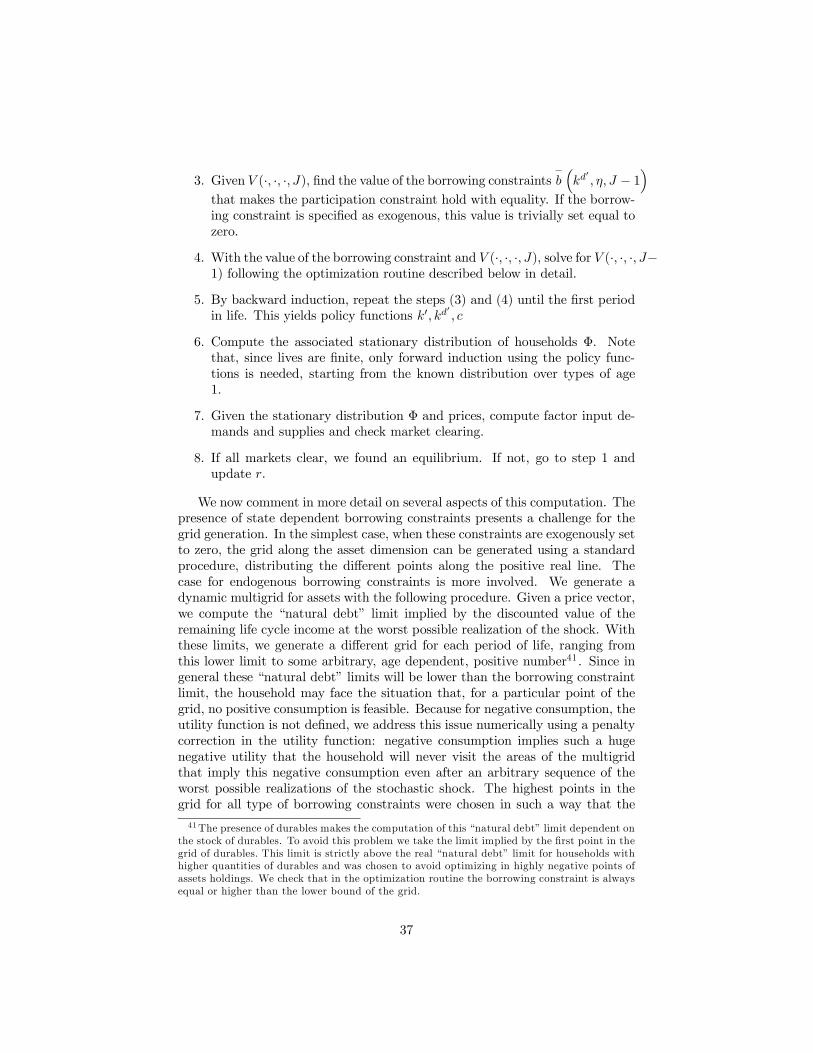
3. Given V (·, ·, ·, J), find the value of the borrowing constraints−b³kd

0, η, J − 1

´that makes the participation constraint hold with equality. If the borrow-ing constraint is specified as exogenous, this value is trivially set equal tozero.

4. With the value of the borrowing constraint and V (·, ·, ·, J), solve for V (·, ·, ·, J−1) following the optimization routine described below in detail.

5. By backward induction, repeat the steps (3) and (4) until the first periodin life. This yields policy functions k0, kd

0, c

6. Compute the associated stationary distribution of households Φ. Notethat, since lives are finite, only forward induction using the policy func-tions is needed, starting from the known distribution over types of age1.

7. Given the stationary distribution Φ and prices, compute factor input de-mands and supplies and check market clearing.

8. If all markets clear, we found an equilibrium. If not, go to step 1 andupdate r.

We now comment in more detail on several aspects of this computation. Thepresence of state dependent borrowing constraints presents a challenge for thegrid generation. In the simplest case, when these constraints are exogenously setto zero, the grid along the asset dimension can be generated using a standardprocedure, distributing the different points along the positive real line. Thecase for endogenous borrowing constraints is more involved. We generate adynamic multigrid for assets with the following procedure. Given a price vector,we compute the “natural debt” limit implied by the discounted value of theremaining life cycle income at the worst possible realization of the shock. Withthese limits, we generate a different grid for each period of life, ranging fromthis lower limit to some arbitrary, age dependent, positive number41. Since ingeneral these “natural debt” limits will be lower than the borrowing constraintlimit, the household may face the situation that, for a particular point of thegrid, no positive consumption is feasible. Because for negative consumption, theutility function is not defined, we address this issue numerically using a penaltycorrection in the utility function: negative consumption implies such a hugenegative utility that the household will never visit the areas of the multigridthat imply this negative consumption even after an arbitrary sequence of theworst possible realizations of the stochastic shock. The highest points in thegrid for all type of borrowing constraints were chosen in such a way that the

41The presence of durables makes the computation of this “natural debt” limit dependent onthe stock of durables. To avoid this problem we take the limit implied by the first point in thegrid of durables. This limit is strictly above the real “natural debt” limit for households withhigher quantities of durables and was chosen to avoid optimizing in highly negative points ofassets holdings. We check that in the optimization routine the borrowing constraint is alwaysequal or higher than the lower bound of the grid.

37

stationary distribution Φ does not put mass in these points. The distributionof point in the grid is uniform.

Finding the level of the borrowing constraint−b at time j amounts to invert

the value function V (·, ·, η0, j + 1) along its first dimension. To do so, we solvethe root of the linear equation V

³·, kd0 , η0, j + 1

´− V (0, 0, η0, j + 1) at each

point of the grid of durables and each possible point η0. Then, since we arelooking for the tightest of borrowing constraint values in the stochastic incomeprocess, we find the vector of maximum values in η0 for each possible choiceof durables stock. This vector contains the value of the borrowing constraint−b³kd

0, η, j + 1

´evaluated at each point in the durables grid, for each η and each

age.With this vector as an input, the optimization routine searches on the grid

of durables and performs a Quasi-Newton update42 on asset holdings condi-tional on each point of the durables grid except for values of the asset holdingclose to the borrowing constraints. For these values we substitute the Quasi-Newton with a variant of the bisection method. This change allows for a correcttreatment of the borrowing constraint in which the derivative of the objectivefunction is not zero. We computed the needed numerical derivatives using a for-ward scheme. To improve efficiency, we tried a two dimensional Newton searchinstead of the combination of grid search and Quasi-Newton. This alternative,however, was not adopted because of numerical instability problems.Where needed, we use a simple linear or bilinear interpolation scheme. As

a robustness check, we also tried a cubic spline interpolation with a “not-a-knot” condition. Cubic splines match exactly the function values at the gridpoints with continuous first and second derivatives. The “not-a-knot” condi-tion requires that the third derivative of the spline be continuous in the lastn − 1 and n − 2 points of the grid. We found that this more sophisticated in-terpolation scheme implied outcomes that were virtually indistinguishable fromthe ones reported in the text and resulted in an important degradation of timeperformance.In order to simulate the stationary distribution Φ and life cycle profiles and

since we store only finite-dimensional arrays, an individual choice k0¡k, kd, η, j

¢is interpreted to choose asset holdings k1 and k2 with probabilities ν and 1− ν.These probabilities solve the linear equation k0

¡k, kd, η, j

¢= νk1 + (1− ν) k2.

A similar procedure is followed for the durable stock choice. We build averagelife-cycles with a simulation of a cross-section of individuals and check the lawof large numbers with the first two moments of the distribution.All the programs needed for the computation of the model were programed

in Fortran 95 and compiled in Compaq Visual Fortran 6.1 to run on WindowsPC. The computational materials are available upon request from the authors.

42Our most important deviation from the standard Newton-Raphson is that we imposerelatively conservative bounds in the size of the update to avoid overshotings. These boundsproved more reliable than cooling down the algorithm because of the discontinuity in thecomputable objective function caused by the penalty correction.

38

References

[1] Abowd, J.M. and D. Card (1989), “On the Covariance Structure of Earn-ings and Hours Changes”. Econometrica 57, 411-445.

[2] Aiyagari, R. (1994), “Uninsured Idiosyncratic Risk and Aggregate Saving”.Quarterly Journal of Economics 109, 659-684.

[3] Alvarez, F. and U. Jermann (2000), “Efficiency, Equilibrium and AssetPricing with Risk of Default”. Econometrica 68, 775-797.

[4] Attanasio, O. P. and M. Browning (1995), “Consumption over the LifeCycle and over the Business Cycle”. American Economic Review 85, 1118-1137.

[5] Attanasio, O.P., J. Banks, C. Meghir and G. Weber (1999), “Humps andBumps in Lifetime Consumption”. Journal of Business and Economics 17,22-35.

[6] Attanasio, O., P.K. Goldberg and E. Kyriazidou (2000), “Credit Con-straints in the Market for Consumer Durables; Evidence from Microdataon Car Loans”. NBER Working Paper 7694.

[7] Attanasio, O. and H. Low (2000), “Estimating Euler Equations”, NBERTechnical Working Paper 253.

[8] Attanasio, O. and G. Weber (1995), “Is Consumption Growth Consistentwith Intertemporal Optimization? Evidence for the Consumer ExpenditureSurvey”. Journal of Political Economy 103, 1121-1157.

[9] Azariadis, C. and L. Lambertini (2000), “Volatility in an Economy withTemporary Default Penalties”. mimeo.

[10] Barrow, L. and L. McGranahan (2000), “The Effects of the Earned In-come Credit on the Seasonality of Household Expenditures”. National TaxJournal, forthcoming.

[11] Bewley, T. (1986), “Stationary Monetary Equilibrium with a Continuumof Independently Fluctuating Consumers”, in W. Hildenbrand and A. Mas-Colell (eds) Contributions to Mathematical Economics in Honor of GerardDebreu, North Holland.

[12] Blundell, R., M. Browning and C. Meghir (1994), “Consumer Demand andthe Life-Cycle Allocation of Household Expenditures”. Review of EconomicStudies 61, 57-80.

[13] Browning, M., A. Deaton and M. Irish (1985), “A Profitable Approach toLabor Supply and Commodity Demands over the Life-Cycle”. Economet-rica, 53, 503-543.

39

[14] Carroll, C. (1992), “The Buffer-Stock Theory of Saving: Some Macroeco-nomic Evidence”. Brookings Papers on Economic Activity, 23, 61-156.

[15] Carroll, C. (1997a), “Buffer-Stuck Saving and the Life Cycle/PermanentIncome Hypothesis”. Quarterly Journal of Economics, 112, 1-55.

[16] Carroll, C. (1997b), “Death to the Log-Linearized Consumption EulerEquation! (And Very Poor Health to the Second-Order Approximation)”.NBER Working Paper 6298.

[17] Chah, E., V. Ramey and R. Starr (1995), “Liquidity Constraints and In-tertemporal Consumer Optimization: Theory and Evidence from DurableGoods”. Journal of Money, Credit and Banking 27, 272-287.

[18] Conesa, J.C. and D. Krueger (1999), “Social Security Reform with Hetero-geneous Agents”. Review of Economic Dynamics 2, 757-795.

[19] Deaton, A. (1985), ”Panel Data from Time Series of Cross-Sections”. Jour-nal of Econometrics 30, 109-126.

[20] Deaton, A. (1991), “Saving and Liquidity Constraints”. Econometrica, 59,1221-1248.

[21] Deaton, A. (1992), Understanding Consumption. Oxford University Press.

[22] Dynan, K. E., J. Skinner and S. Zeldes (2000), “Do the Rich Save More?”.NBER Working Paper 7906.

[23] Eberly, J. (1994), “Adjustment of Consumers’ Durables Stocks: Evidencefrom Automobile Purchases”. Journal of Political Economy 102, 403-436.

[24] Eichenbaum, M. and L.P. Hansen (1990), “Estimating Models with In-tertemporal Substitution Using Aggregate Time Series Data”. Journal ofBusiness and Economic Statistics 8, 53-69.

[25] Faber, J. F. (1982), “Life tables for the United States: 1900-2050”, Actu-arial Study No 87, U.S. Department of Health and Human Services.

[26] Feldman, M. and C. Gilles (1985), “An Expository Note on Individual Riskwithout Aggregate Uncertainty”. Journal of Economic Theory 35(1), 26-32.

[27] Fernández-Villaverde, J. and D. Krueger (2000), “Business Cycle, Con-sumption and Durable Goods”, work in progress.

[28] Fernández-Villaverde, J. and D. Krueger (2002), “Consumption of Non-durables and Durables, and the Allocation of Assets over the Life Cycle:Empirical Findings from Micro Data,” mimeo.

[29] Flavin, M. and T. Yamashita (2000), “Owner-Occupied Housing and theComposition of the Household Portfolio”. NBER Working Paper 6389.

40

[30] Ghez, G.R. and G. Becker, (1975), The Allocation of Time and Goods overthe Life Cycle. Columbia University Press for the NBER.

[31] Gottschalk, P. and R. Moffitt (1994). “The Growth of Earnings Instabilityin the U.S. Labor Market”. Brookings Papers on Economic Activity, 217-272.

[32] Gourinchas, P.O. and J. A. Parker (1999), “Consumption over the LifeCycle”. NBER Working Paper 7271.

[33] Greenwood, J., R. Rogerson and R. Wright (1995), “Household Productionin Real Business Cycle Theory” in T.F. Cooley (ed) Frontiers of BusinessCycle Research. Princeton University Press.

[34] Grossman, S. and G. Laroque (1990), “Asset Pricing and Optimal PortfolioChoice in the Presence of Illiquid Durable Consumption Goods”. Econo-metrica, 58, 25-51.

[35] Hall, Peter (1992), The Bootstrap and Edgeworth Expansion. Springer-Verlag.

[36] Hansen, G. D. (1993), “The Cyclical and Secular Behavior of the LaborInput: Comparing Efficiency Units and Hours Worked”. Journal of AppliedEconometrics, 8, 71-80.

[37] Härdle, W. (1990), Applied Nonparametric Regression. Cambridge Univer-sity Press.

[38] Härdle, W, H. Liang and J. Gao, (2000) Partially Linear Models, PhysicaVerlag, Heidelberg.

[39] Heckman, J.J. and R. Robb (1985), “Alternative Methods for Evaluatingthe Impact of Interventions” in J.J. Heckman and B. Singer (eds), Longi-tudinal Analysis of Labor Market Data. Cambridge University Press.

[40] Horowitz, . (2001), “The Bootstrap and Hypothesis Tests in Econometrics,”Journal of Econometrics, 100, 37-40.

[41] Huggett, M. (1993), “The Risk-Free Rate in Heterogeneous-AgentIncomplete-Insurance Economies”. Journal of Economic Dynamics andControl, 17, 953-969.

[42] Kehoe, T. and D. Levine (1993), “Debt Constrained Asset Markets”. Re-view of Economic Studies, 60, 865-888.

[43] Kennickell, A.B. and W.R. Lousie (1999), “Consistent Weight Design forthe 1989, 1992 and 1995 SCFs and the Distribution of Wealth”. Review ofIncome and Wealth, 45, 193-215.

[44] Kocherlakota, N. (1996), “Implications of Efficient Risk Sharing withoutCommitment”. Review of Economic Studies 63, 595-609.

41

[45] Krueger, D. and F. Perri (1999), “Risk Sharing: Private Insurance Mar-kets or Redistributive Taxes?”. Federal Reserve Bank of Minneapolis StaffReport 262.

[46] Krueger, D. and F. Perri (2001), “Does Income Inequality Lead to Con-sumption Inequality? Empirical Findings and a Theoretical Explanation,”mimeo.

[47] Krusell, P. and A. Smith (1998), “Income and Wealth Heterogeneity in theMacroeconomy”. Journal of Political Economy 106, 867-96.

[48] Ludgvison, S. and Paxson, C. (1999), “Approximation Bias in LinearizedEuler Equations”. NBER Technical Working Paper 236.

[49] Lustig, H. (2000), “Secured Lending and Asset Prices,” mimeo, StanfordUniversity.

[50] McGrattan, E. R. Rogerson and R. Wright (1997), “An Equilibrium Modelof Business Cycle with Household Production and Fiscal Policy”. Interna-tional Economic Review 38, 267-290.

[51] McGrattan, E. and E.C. Prescott (2000), “Is the Stock Market Overval-ued?”. Mimeo, Federal Reserve Bank of Minneapolis.

[52] Ogaki, M. and C.M. Reinhart (1998), “Measuring Intertemporal Substi-tution: The Role of Durable Goods”. Journal of Political Economy 106,1078-1098.

[53] Platania, J. and D. Schlagenauf (2000), “Housing and Asset Holding in aDynamic General Equilibrium Model,” mimeo.

[54] Rupert, P., R. Rogerson and Randall Wright (1995), “Estimating Substi-tution Elasticities in Household Production Models”. Economic Theory 6,179-193.

[55] Schechtman, J. (1976), “An Income Fluctuation Problem”. Journal of Eco-nomic Theory 12, 218-241.

[56] Schechtman, J. and Escudero, V. (1977), “Some Results on “An IncomeFluctuation Problem”. Journal of Economic Theory 16, 151-166.

[57] Storesletten, K., C. Telmer and A. Yaron (1999), “Asset Pricing with Id-iosyncratic Risk and Overlapping Generations”. Mimeo.

[58] Tauchen, G. and R. Hussey (1991), “Quadrature-Based Methods for Ob-taining Approximate Solutions to Nonlinear Asset Pricing Models”. Econo-metrica 59, 371-396.

[59] Tracy, J., H. Schneider and S. Chan (1999), “Are Stocks Overtaking RealEstate in Household Portfolios?”. Current Issues in Economics and Fi-nance, Federal Reserve Bank of New York, 5(5).

42

0 20 40 60 80 100400

500

600

700

800

900

1000

Figure 2.4a: Household size = 1,95% confidence interval

0 20 40 60 80 100400

500

600

700

800

900

1000

Figure 2.4b: Household size = 1,widest confidence interval

0 20 40 60 80 100400

500

600

700

800

900

1000

Figure 2.4c: Household size = 1,95% confidence band

0 20 40 60 80 100400

500

600

700

800

900

1000

Figure 2.4d: Household size = 1,all simulations

20 30 40 50 60 70 80 900

50

100

150

200

250

300

350

400

450Figure 2.9: Households Net Worth, 1995 SCF

age

Tho

usan

ds o

f 199

8 do

llars

20 30 40 50 60 70 80 900

20

40

60

80

100

120

140

160

180Figure 2.11: Median Households Assets, 1995 SCF

age

Tho

usan

ds o

f 199

8 do

llars

0 10 20 30 40 50 60 70 80 90 1000

10

20

30

40

50

60

70Figure 2.10: Households Assets Distribution by Wealth, 1995 SCF

Wealth Percentile

Per

cent

age

mean

median

Real Estate

Equity Primary Residence

Total

20 30 40 50 60 70 80 90 1000.75

0.8

0.85

0.9

0.95

1Figure 4.1: Conditional Survival Probabilities

Age

Con

ditio

nal S

urvi

val P

roba

bilit

ies

20 30 40 50 60 70 80 90 1000

0.2

0.4

0.6

0.8

1

1.2

1.4

1.6

1.8

2

Age

Ave

rage

Lab

or In

com

e, A

vera

ge C

onsu

mpt

ion

Figure 5.1: Life Cycle Pattern of Labor Income and Nondurable Consumption

Labor IncomeConsumption

20 30 40 50 60 70 80 90 100-5

0

5

10

15

20

Age

Ave

rage

Dur

able

s, F

inan

cial

Ass

ets

and

Tot

al W

ealth

Figure 5.2: Life Cycle Pattern of Consumer Durables, Financial Wealth and Total Wealth

Durables Financial AssetsTotal Wealth

20 30 40 50 60 70 80 90 1000

0.5

1

1.5

2

2.5

3Figure 5.3: Average Stock of Durables

Age

aver

age

stoc

k of

dur

able

s

20 30 40 50 60 70 80 90 100-0.05

0

0.05

0.1

0.15

0.2

0.25

0.3

0.35

0.4

0.45Figure 5.4: Average Expenditure on Durables

Age

aver

age

expe

nditu

re o

n du

rabl

es

20 30 40 50 60 70 80 90 1000.2

0.4

0.6

0.8

1

1.2

1.4

1.6

1.8

2

2.2Figure 5.5: Some Simulated Life Cycle Consumption Profiles

Age

Sim

ulat

ed P

rofil

es

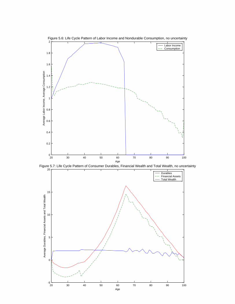
20 30 40 50 60 70 80 90 1000

0.2

0.4

0.6

0.8

1

1.2

1.4

1.6

1.8

2

Age

Ave

rage

Lab

or In

com

e, A

vera

ge C

onsu

mpt

ion

Figure 5.6: Life Cycle Pattern of Labor Income and Nondurable Consumption, no uncertainty

Labor IncomeConsumption

20 30 40 50 60 70 80 90 100-5

0

5

10

15

20

Age

Ave

rage

Dur

able

s, F

inan

cial

Ass

ets

and

Tot

al W

ealth

Figure 5.7: Life Cycle Pattern of Consumer Durables, Financial Wealth and Total Wealth, no uncertainty

Durables Financial AssetsTotal Wealth

20 30 40 50 60 70 80 90 100−5

0

5

10

15

20

25

30Figure 5.8: Simulated and Average Life Cycle Pattern of Financial Assets

Age

Ave

rage

Lab

or In

com

e, S

imul

ated

Fin

anci

al A

sset

s

Average Low Income High Income

20 30 40 50 60 70 80 90 1000

0.2

0.4

0.6

0.8

1

1.2

1.4

1.6

1.8

2

Age

Ave

rage

Lab

or In

com

e, A

vera

ge C

onsu

mpt

ion

Figure 6.1: Life Cycle Pattern of Labor Income and Nondurable Consumption

Labor IncomeConsumption

20 30 40 50 60 70 80 90 1000

2

4

6

8

10

12

14

16

Age

Ave

rage

Dur

able

s, F

inan

cial

Ass

ets

and

Tot

al W

ealth

Figure 6.2: Life Cycle Pattern of Consumer Durables, Financial Wealth and Total Wealth

Durables Financial AssetsTotal Wealth

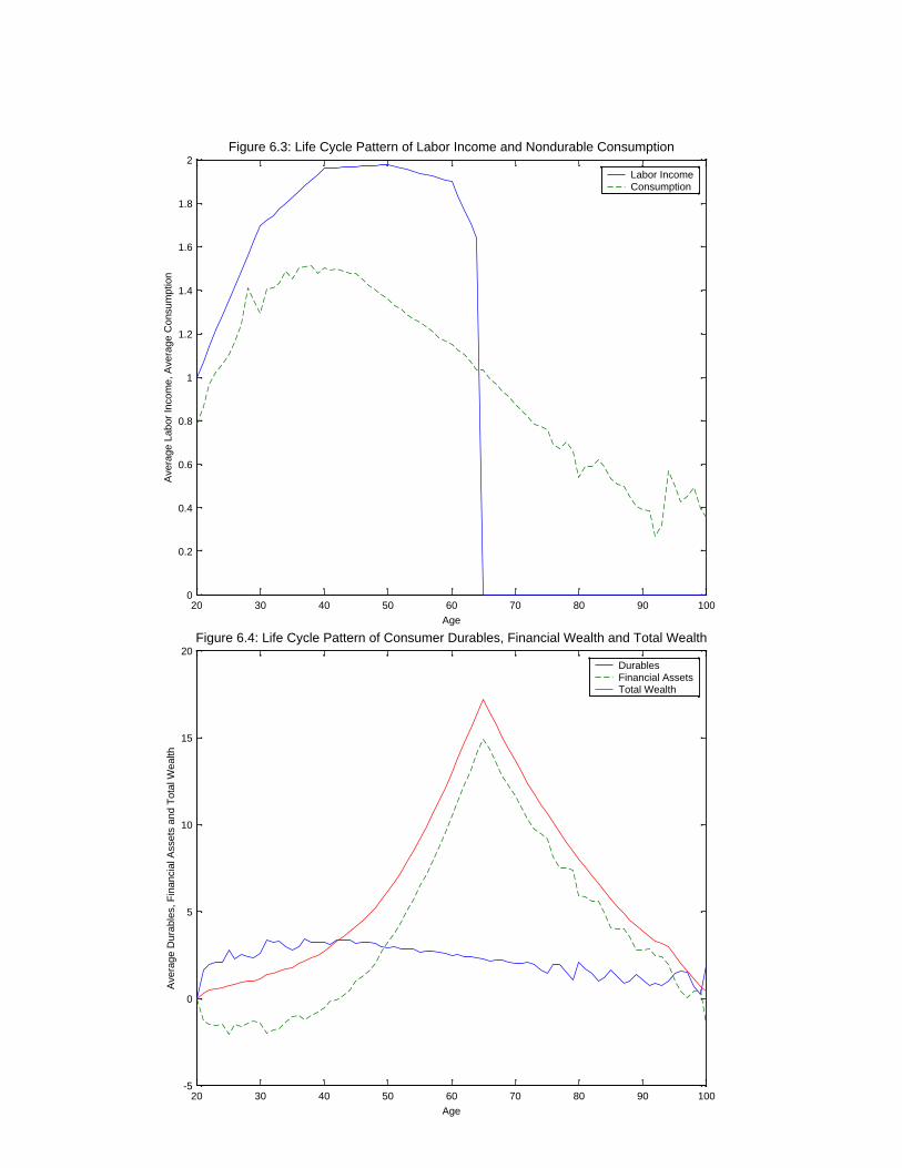
20 30 40 50 60 70 80 90 1000

0.2

0.4

0.6

0.8

1

1.2

1.4

1.6

1.8

2

Age

Ave

rage

Lab

or In

com

e, A

vera

ge C

onsu

mpt

ion

Figure 6.3: Life Cycle Pattern of Labor Income and Nondurable Consumption

Labor IncomeConsumption

20 30 40 50 60 70 80 90 100-5

0

5

10

15

20

Age

Ave

rage

Dur

able

s, F

inan

cial

Ass

ets

and

Tot

al W

ealth

Figure 6.4: Life Cycle Pattern of Consumer Durables, Financial Wealth and Total Wealth

Durables Financial AssetsTotal Wealth