Sierra Nevada Network Rivers Monitoring Protocol · NPS XXXXXX, March 2012 . ... An example of the summary statistics table that is included in the biennial ... Sierra Nevada Network

National Park Service U.S. Department of the Interior Natural Resource Stewardship and Science

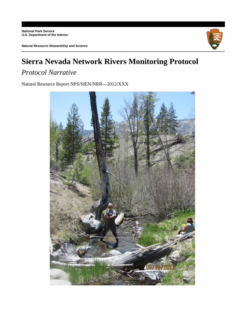
Sierra Nevada Network Rivers Monitoring Protocol Protocol Narrative Natural Resource Report NPS/SIEN/NRR—2012/XXX

ON THE COVER DEPO Protection Ranger John Anderson performing a discharge measurement at Boundary Creek in Devils Postpile National Monument Photograph by: Jennie Skancke – Sierra Nevada Network

Sierra Nevada Network Rivers Monitoring Protocol Protocol Narrative Natural Resource Report NPS/SIEN/NRR—2012/XXX

Jennie Skancke Alice Chung-MacCoubrey National Park Service, Sierra Nevada Network Inventory & Monitoring Program Sequoia and Kings Canyon National Parks 47050 Generals Hwy Three Rivers, CA 93271

Leslie Chow

National Park Service, Sierra Nevada Network Inventory & Monitoring Program Yosemite Field Station P.O. Box 700 El Portal, CA 95318

March 2012

U.S. Department of the Interior National Park Service Natural Resource Stewardship and Science Fort Collins, Colorado

ii

The National Park Service, Natural Resource Stewardship and Science office in Fort Collins, Colorado publishes a range of reports that address natural resource topics of interest and applicability to a broad audience in the National Park Service and others in natural resource management, including scientists, conservation and environmental constituencies, and the public.

The Natural Resource Report Series is used to disseminate high-priority, current natural resource management information with managerial application. The series targets a general, diverse audience, and may contain NPS policy considerations or address sensitive issues of management applicability.

All manuscripts in the series receive the appropriate level of peer review to ensure that the information is scientifically credible, technically accurate, appropriately written for the intended audience, and designed and published in a professional manner.

Peer review manager: choose one or combine and edit multiple pieces from the numbered statements below to best describe the type of peer review performed. The result should be in regular paragraph format and the same font and color as all other text on this page. Make sure to delete all explanatory and unwanted text currently shown in blue italic font.

1. This report received informal peer review by subject-matter experts who were not directly involved in the collection, analysis, or reporting of the data.

2. Data in this report were collected and analyzed using methods based on established, peer-reviewed protocols and were analyzed and interpreted within the guidelines of the protocols.

3. This report received formal peer review by subject-matter experts who were not directly involved in the collection, analysis, or reporting of the data, and whose background and expertise put them on par technically and scientifically with the authors of the information.

4. This report received formal, high-level peer review based on the importance of its content, or its potentially controversial or precedent-setting nature. Peer review was conducted by highly qualified individuals with subject area technical expertise and was overseen by a peer review manager.

Views, statements, findings, conclusions, recommendations, and data in this report do not necessarily reflect views and policies of the National Park Service, U.S. Department of the Interior. Mention of trade names or commercial products does not constitute endorsement or recommendation for use by the U.S. Government.

This report is available from the Sierra Nevada Network website (http://science.nature.nps.gov/im/units/sien) and the Natural Resource Publications Management website (http://www.nature.nps.gov/publications/nrpm).

Please cite this publication as:

Skancke, J. R., A. L. Chung-MacCoubrey, and L. Chow. 2012. Sierra Nevada Network Rivers Monitoring Protocol: Protocol Narrative. Natural Resource Report NPS/SIEN/NRR—2012/XXX. National Park Service, Fort Collins, Colorado.

NPS XXXXXX, March 2012

http://science.nature.nps.gov/im/units/sien�

http://www.nature.nps.gov/publications/nrpm�

iii

Contents Page

Figures........................................................................................................................................... vii

Tables ............................................................................................................................................. ix

Appendices ..................................................................................................................................... xi

Standard Operating Procedures.................................................................................................... xiii

Executive Summary ...................................................................................................................... xv

Acknowledgments....................................................................................................................... xvii

List of Terms and Acronyms ....................................................................................................... xix

Revision History Log ................................................................................................................... xxi

1. Background and Objectives ........................................................................................................ 1

1.1 Sierra Nevada Network Surface Water Monitoring .......................................................... 2

1.2 Rationale for Monitoring Rivers ........................................................................................ 3

1.2.1 Sierra Nevada Hydrology .......................................................................................... 3

1.2.2 Sierra Nevada Surface Water Quality ..................................................................... 10

1.3 Thresholds and Guidelines for Management ................................................................... 11

1.3.1 State and federal standards and guidance ............................................................... 11

1.3.2 SEKI-specific thresholds .......................................................................................... 12

1.4 Monitoring Questions and Measurable Objectives .......................................................... 14

1.4.1 Monitoring Questions .............................................................................................. 14

1.4.2 Primary Measureable Objectives ............................................................................ 14

1.3.3. Monitoring Approach.............................................................................................. 15

1.4.3 SIEN Vital Signs Integration and Linkages ............................................................. 15

1.5 Major Watersheds of the Sierra Nevada Network ........................................................... 16

1.5.1 Yosemite National Park ........................................................................................... 16

iv

1.5.2 Devils Postpile National Monument ........................................................................ 20

1.5.3 Sequoia and Kings Canyon National Parks ............................................................ 22

2. Sampling Design ....................................................................................................................... 27

2.1 Monitoring Approach ...................................................................................................... 27

2.2 Station Selection .............................................................................................................. 29

2.2.2 Station Specifics ....................................................................................................... 32

Stations supported or operated by SIEN .................................................................... 32

Other station information ........................................................................................... 33

2.3 Selected Measures ........................................................................................................... 34

2.3.1 Hydrologic parameters ............................................................................................ 34

2.3.2 Water chemistry parameters .................................................................................... 36

2.4 Power and Trend Analysis ............................................................................................... 36

2.4.1 Methods .................................................................................................................... 37

2.4.2 Results ...................................................................................................................... 37

3. Field Methods ........................................................................................................................... 39

3.1 Routine Station Visits ...................................................................................................... 39

3.1.1 Discharge Measurements......................................................................................... 41

3.2 Station improvement and maintenance ............................................................................ 44

3.2.1 SIEN-operated stations ............................................................................................ 44

3.2.2 Other stations ........................................................................................................... 45

4. Data Collection and Acquisition ............................................................................................... 47

4.1 Data Sources .................................................................................................................... 47

4.2 Data Collection and Acquisition ...................................................................................... 49

5. Data Management ..................................................................................................................... 51

5.1 Aquarius Software and SQL Server Database ................................................................. 52

v

5.2 Data Processing and Storage ........................................................................................... 55

5.2.1 Discharge and water level data from SIEN-operated gages ................................... 55

5.2.2 Mean daily discharge acquired from streamgages operated or reviewed by USGS ................................................................................................................................. 55

5.2.3 Mean daily discharge acquired from streamgage operators ................................... 55

5.2.4 Continuous water temperature data ........................................................................ 55

5.3 Metadata Procedures ........................................................................................................ 56

5.4 Data Standards ................................................................................................................. 56

5.4.1 Accuracy and Detection Limits ................................................................................ 56

5.4.2 Minimum Detectable Differences ............................................................................ 56

5.5 Quality Assurance and Quality Control Procedures ........................................................ 57

6. Data Analysis and Reporting .................................................................................................... 59

6.1 Hydrologic Data Analysis ................................................................................................ 59

6.1.1 Summary Analysis .................................................................................................... 59

6.1.2 Trend Analysis ......................................................................................................... 63

6.1.3 Additional hydrologic analysis ................................................................................ 64

6.2 Water Quality Data Analysis ........................................................................................... 64

6.3 Reporting ......................................................................................................................... 65

6.3.1 Summary reports ...................................................................................................... 65

6.3.2 Comprehensive Status and Trend Reports ............................................................... 66

7. Personnel Requirements and Training ...................................................................................... 67

7.1 Roles and Responsibilities ............................................................................................... 67

7.2 Annual schedule of SIEN responsibilities ....................................................................... 68

7.3 Park Contributions ........................................................................................................... 68

7.4 Qualifications and Training ............................................................................................. 68

8. Operational Requirements ........................................................................................................ 71

vi

8.1 Operation of the DEPO streamgage ................................................................................ 72

8.2 Operation of other selected streamgages ......................................................................... 72

8.2.1 Start-up costs ........................................................................................................... 72

8.2.2 Recurring Costs ....................................................................................................... 73

9. Literature Cited ......................................................................................................................... 75

vii

Figures Page

Figure 1. Sierra Nevada Network parks and major watersheds. 4

Figure 2. An example of the relationship between snow accumulation and snowmelt at the Tenaya Lake snowcourse in the upper Merced Watershed and discharge at the Happy Isles streamgage in the lower portion of the watershed. 7

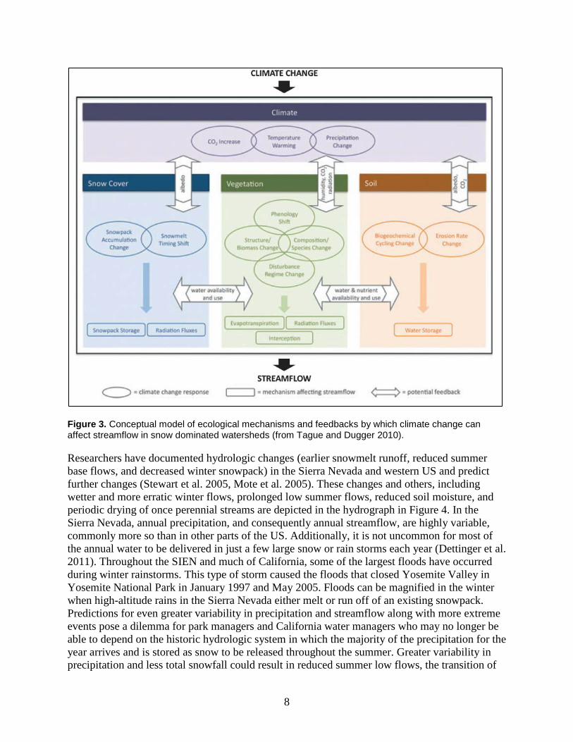
Figure 3. Conceptual model of ecological mechanisms and feedbacks by which climate change can affect streamflow in snow dominated watersheds (from Tague and Dugger 2010). 8

Figure 4. Hydrograph depicting changes in Sierra Nevada hydrology predicted to occur with shifting precipitation dynamics and climate warming. 9

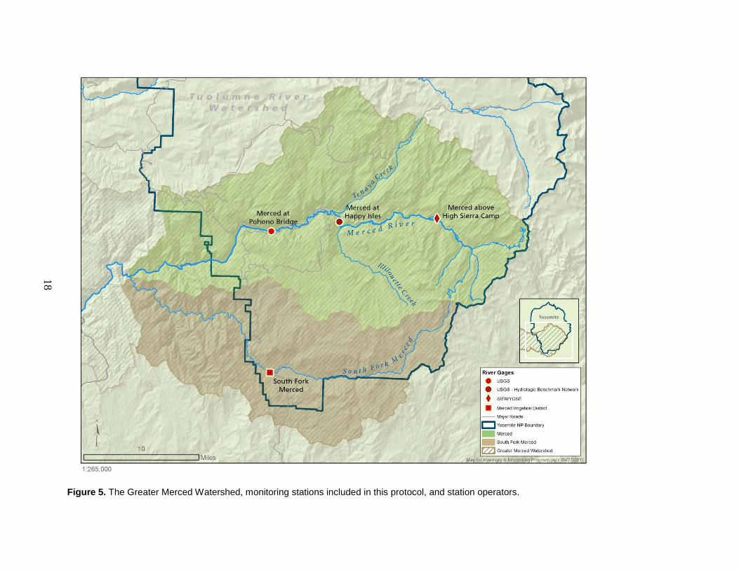
Figure 5. The Greater Merced Watershed, monitoring stations included in this protocol, and station operators. 18

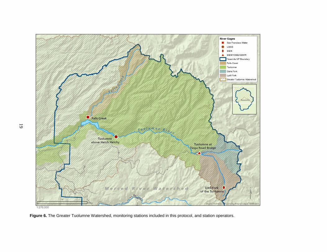
Figure 6. The Greater Tuolumne Watershed, monitoring stations included in this protocol, and station operators. 19

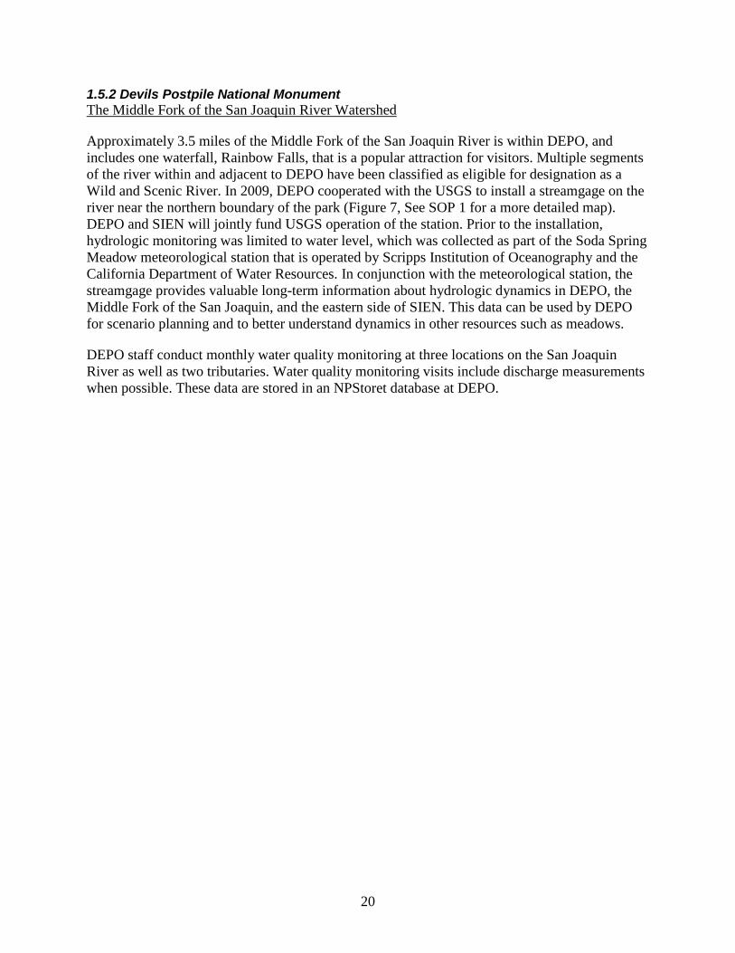
Figure 7. The Middle Fork of the San Joaquin Watershed including the Devils Postpile streamgage. 21

Figure 8. The Greater Kaweah River Watershed, monitoring stations selected for this protocol, and station operators. 23

Figure 9. The Kern River Watershed and Kern River streamgage. 25

Figure 10. The Marble Fork of the Kaweah above Tokopah Falls streamgage and Hydrologic Benchmark Network station. 33

Figure 11. A generalized workflow for office preparation and procedures for streamgage station visits. See SOPs 3, 4, and 5 for more details. 40

Figure 12. Definition sketch of the current meter midsection method of computing cross-section area for discharge measurements (from Turnipseed and Sauer 2010). 42

Figure 13. Typical staff gage with numbers for reading water depth at the Tuolumne River at Tioga Road Bridge streamgage. 43

Figure 14. Temporary marker for measuring water depth at the Lyell Fork below Maclure streamgage. 44

Figure 15. Representation of data sources, types, processing mechanisms and storage locations used for this protocol. 50

viii

Figure 16. Steps in the data and project information cycle from data acquisition to archiving. Figure from the North Coast and Cascades Network. 51

Figure 17. View of the Aquarius Springboard, the starting point for establishing locations, uploading and managing data. 54

Figure 18. An example of a hydrograph that will be included in the biennial summary report. 60

Figure 19. Flood frequency curve for the Merced River at Pohono Bridge streamgage. 62

ix

Tables Page

Table 1. Area, elevation and wilderness statistics for parks within the Sierra Nevada Network........................................................................................................................................... 1

Table 2. Mountain hydrology parameters monitored by this protocol that can serve as indicators of change in runoff timing.............................................................................................. 6

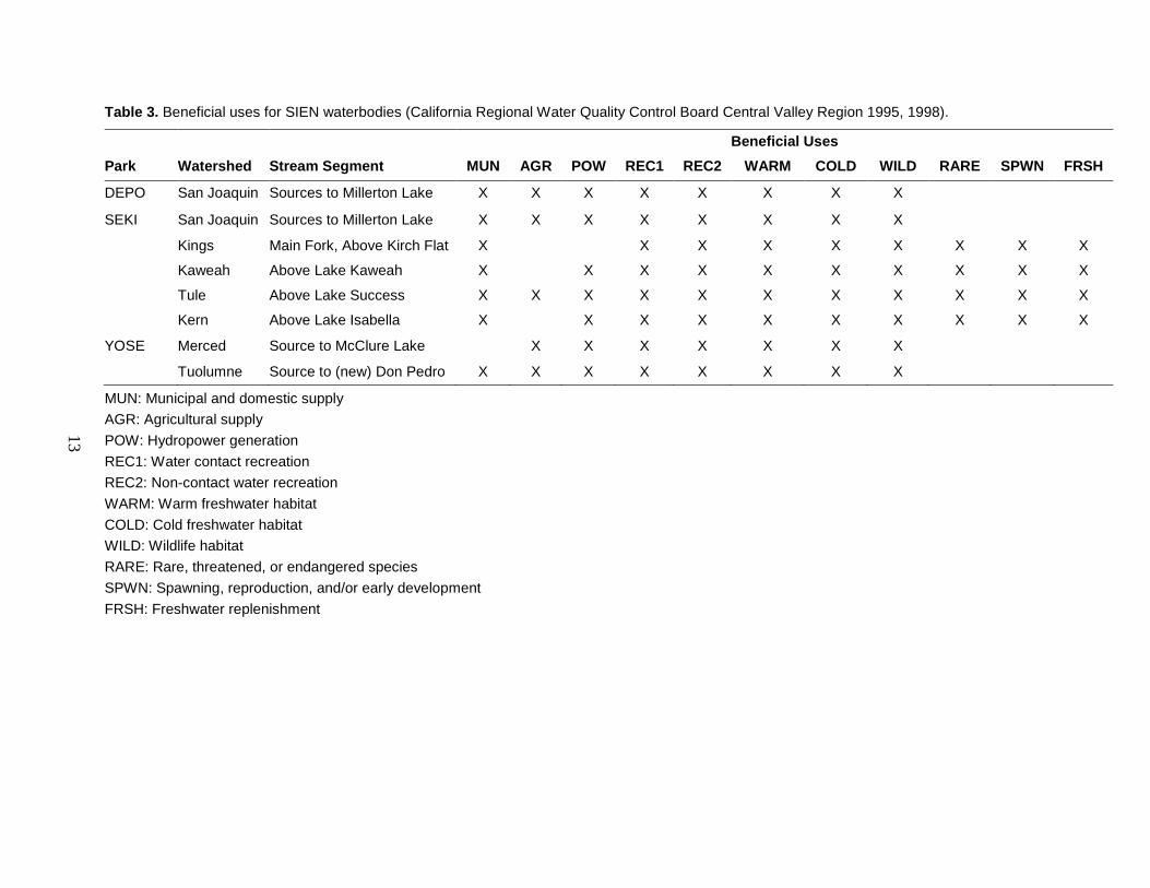
Table 3. Beneficial uses for SIEN waterbodies (California Regional Water Quality Control Board Central Valley Region 1995, 1998). .................................................................................. 13

Table 4. The locations and operators of the 14 existing streamflow gaging stations in the SIEN parks that will be included in reports, as part of this protocol. ........................................... 31

Table 5. Hydrologic parameters and statistics measured or calculated for SIEN reports. ........... 35

Table 6. Water chemistry parameters collected or analyzed for SIEN reports. ........................... 36

Table 7. Standard Operating Procedures (SOPs) pertinent to field operations. ........................... 39

Table 8. Streamflow gaging stations, operators and data retrieval processes. ............................. 48

Table 9. Standard Operating Procedures pertinent to data management activities. ..................... 52

Table 10. An example of the summary statistics table that is included in the biennial summary reports. Data below are fabricated. ............................................................................... 61

Table 11. Streamgages that are located along an elevational gradient within SIEN watersheds. .................................................................................................................................... 64

Table 12. Reporting schedule for rivers monitoring during the first six years. Schedule repeats with a trend report every four years and status report every two years. ........................... 66

Table 13. Assigned staff, specific responsibilities, and time estimates for rivers monitoring. .... 67

Table 14. Routine field and office tasks and approximate timeframe for completion. ................ 68

Table 15. Annual SIEN budget for river monitoring, including start-up costs for first 4 years. Subtotals are provided for personnel and operations costs. ............................................... 71

Table 16. Start-up equipment for first four years of river monitoring ......................................... 73

xi

Appendices Page

Appendix A. Important Data Sets, Monitoring Programs and Partnerships ................................. 83

Appendix B. Recommendations for Expanded Surface Water Monitoring ................................. 87

Appendix C. Power Analysis of Trends in Streamflow Parameters for the Sierra Nevada Network......................................................................................................................................... 89

Appendix D. Southern California Edison Infrastructure and Streamgage Information .............. 131

Appendix E. Administrative Record ........................................................................................... 133

Appendix F. Data Dictionary for SQL Server Database............................................................. 135

xiii

Standard Operating Procedures SOP 1. Streamgage Station Descriptions

SOP 2. Training and Annual Schedule of Activities

SOP 3. Procedures and Equipment for Station Visits

SOP 4. Methods for Streamflow Discharge Measurements

SOP 5. Safety Procedures

SOP 6. Acquiring Water Quality and Streamflow Data from Streamgage Operators

SOP 7. Data Management

SOP 8. Data Analysis

SOP 9. Reporting

SOP 10. Quality Assurance Plan

SOP 11. Revising the Protocol

xv

Executive Summary The National Park Service (NPS) Inventory & Monitoring (I&M) Program was established in 2000 as part of the Natural Resource Challenge, a long-term strategy to improve park management by increasing access to and reliance on high-quality scientific information. The Sierra Nevada Network (SIEN) is one of 32 I&M networks that will develop and provide scientifically credible information on the status and long-term trends in selected Vital Signs, or indicators of ecosystem condition. The SIEN is comprised of four units: Devils Postpile National Monument (DEPO), Sequoia & Kings Canyon National Park (jointly administered units that are referred to as SEKI, or individually as SEQU & KICA), and Yosemite National Park (YOSE). The SIEN Vital Signs Monitoring Plan (Mutch et al. 2008) identified 13 high priority vital signs for which long-term monitoring protocols would be developed. Two of these vital signs, surface water dynamics and water chemistry, are included in this protocol.

The overall goal of the SIEN I&M Program is to provide park managers with information needed to make decisions that will maintain the integrity of Sierra Nevada ecosystems. The monitoring objectives in this protocol are to report on the status of and to detect long-term trends in surface hydrology and water quality (freshwater chemistry) of Sierra Nevada rivers. The protocol includes streamgages operated by the SIEN and other agencies. A major strength of our approach is that it will collect data from a variety of sources into a central location and analyze and report resulting information to the parks for management purposes and for sharing with academic researchers, state agencies, and other cooperators. The SIEN will provide the services of summarizing the data, calculating statistics that may be indicators of change, and interpreting the findings to park staff so they may find successful solutions to address or mitigate environmental challenges.

The primary focus of this protocol is the hydrology of rivers (i.e., streamflow timing and volume) in the SIEN. We will operate or support several stations and acquire the mean daily discharge values from stations that are operated by other agencies, such as the USGS and Southern California Edison Electric Company. We will use the mean daily discharge values from all stations to calculate up to 14 additional hydrologic parameters for each station (i.e., number of days to the onset of snowmelt). We have selected existing stations for this protocol. Although SIEN will not establish new stations, we may incorporate new stations that are installed and operated by others if the data contribute to our protocol objectives. There are 14 streamgages from which data will be collected, stored, and reported.

Water chemistry is a secondary component of this protocol. We will collect 15-minute water temperature measurements at stations (where possible) and analyze temperature data for trends every four years. Additionally, we will analyze and report on water chemistry data from two long-term USGS water quality monitoring stations on the Kaweah and Merced Rivers. These data will be analyzed using the same methods and on the same schedule as the water quality trend reports for the SIEN lakes monitoring program.

This protocol has two reporting products, hydrologic summaries of each year (produced on a biennial basis) and comprehensive trend reports (produced every four years). Biennial hydrologic summaries will provide standardized information including: hydrographs of daily mean discharge, low and high flow values, calculated snowmelt runoff statistics, and photographs.

xvi

Long-term trend reports will include similar information as the biennial reports with the addition of flow-duration curves, flood frequency analyses, and the assessment of trends in selected hydrologic parameters.

This protocol provides a basic summary of current and historic river monitoring in the Sierra Nevada, describes hydrologic and water chemistry measures selected for monitoring, articulates our monitoring objectives and goals, summarizes our approach to station selection, data collection, acquisition, analysis, management, and reporting, and outlines personnel requirements and operational costs. This protocol also includes standard operating procedures (SOPs) for implementing the protocol and appendices that describe the protocol development process, power analyses, historic water data sets in the SIEN, and recommendations for expanded monitoring.

xvii

Acknowledgments

We would like to thank SIEN Physical Scientist Andi Heard, primary author of the SIEN Lakes Protocol, who holds so much knowledge about the history of SIEN protocol development, answered question after question, and paved the way with the Lakes Protocol. Portions of the Lakes Protocol have been duplicated here, including the section on water quality regulations and much of Appendix A. Sandy Graban created the lovely maps in this protocol. Edward (Ned) Andrews provided an analysis and report on streamflow and snowpack status and trends that is the foundation for large portions of this document. Ned has been very generous with his time, explaining many of the data analysis methods that will be used for this protocol and answering long lists of questions. Leigh Ann Harrod Starcevich and Stephanie Kane contributed the power analysis for this report which is included as Appendix C of this narrative. We would like to acknowledge the water work group, who were among our greatest partners - Jim Roche at Yosemite and Annie Esperanza, Danny Boiano, and Harold Werner at SEKI as well as Andi Heard with the SIEN. Most of the decisions that made this protocol come together were made by the workgroup. We believe that developing the protocol with limited funding was more difficult than working with a larger amount of money, particularly because the work group members are so passionate and dedicated to the resources and are great advocates for long-term monitoring. The following individuals should be thanked in advance because our reports will depend upon data collected and provided by them: Dan Garrigue at Sierra Hydrographics; Kevin Skeen, John Melack, and Jim Sickman at the University of California; Derrik Tito at Southern California Edison, who has been so great, digging up old records and explaining the ins and outs of the diversion system at SEKI; Dave Clow and Heidi Roop at the USGS and Jessica Lundquist at University of Washington have answered innumerable questions and provided excellent advice on a number of issues. There are so many other organizations and cooperators doing valuable work to better understand surface water dynamics in this region who have been very helpful, especially Frank Gehrke from the California Department of Water Resources, Bruce McGurk at San Francisco Water. Some of the content for this protocol came from the San Francisco Network Streamflow Protocol (Fong et al. 2011) and the Southwest Alaska Network Freshwater Flow System Protocol. We thank Darren Fong and the SWAN staff for allowing us to adopt sections of their protocols.

xix

List of Terms and Acronyms CDWR California Department of Water Resources DEPO Devils Postpile National Monument HBN Hydrologic Benchmark Network HHWP Hetch Hetchy Water and Power I & M Inventory and Monitoring Division of the National Park Service KICA Kings Canyon National Park MKT Mann-Kendall Test MID Merced Irrigation District NPS National Park Service NRDS Natural Resources Data Series NRR Natural Resources Report NRTR Natural Resources Technical Report NWIS National Water Information System – Operated by the USGS OLS Ordinary Least Squares ORV Outstandingly Remarkable Value QA/QC Quality Assurance/Quality Control RWQCB Regional Water Quality Control Board SCE Southern California Edison Electric Company Scripps Scripps Institution of Oceanography SEKI Sequoia and Kings Canyon National Parks SEQU Sequoia National Park SF Water San Francisco Water Department SIEN Sierra Nevada Network Inventory & Monitoring Program SKT Seasonal Kendall Test SNEP Sierra Nevada Ecosystem Project SOP Standard Operating Procedure SWAN Southwest Alaska Network UC University of California US ACE US Army Corps of Engineers USGS United States Geological Survey VSMP Vital Signs Monitoring Plan WRD Water Resources Division of the National Park Service WY Water Year YOSE Yosemite National Park

xxi

Revision History Log

This table reflects changes to this document. Version numbers will be incremented by one (e.g., Version 1.3 to Version 2.0) each time there is a significant change in the process and/or changes are made that affect the interpretation of the data. Version numbers will be incremented after the decimal (e.g., Version 1.6 to Version 1.7…1.10….1.21) when there are changes to grammar, spelling, or formatting, or minor modifications in the process that do not affect the interpretation of the data.

Previous Version #

Revision date Author Changes made Section and

paragraph Reason for change New Version #

1

1. Background and Objectives In 2000, the National Park Service (NPS) established the Inventory & Monitoring (I&M) Program to provide scientifically credible information on the status and long-term trends in Vital Signs, or indicators of ecosystem condition, with the overarching goal of supporting park management through increased access to and reliance on high-quality scientific information. The national I&M Program created 32 networks of parks that are linked by geography and shared natural resource characteristics. Within each network, parks are able to share budgets, staffing, and other resources to plan and implement an integrated program. NPS I&M networks share five common goals (Fancy 2011):

1. Inventory the natural resources and park ecosystems under NPS stewardship to determine their nature and status

2. Monitor park ecosystems to better understand their dynamic nature and condition and to provide reference points for comparisons with other, altered environments

3. Establish natural resource inventory and monitoring as a standard practice throughout the NPS system that transcends traditional program, activity, and funding boundaries

4. Integrate natural resource inventory and monitoring information into NPS planning, management, and decision making

5. Share NPS accomplishments and information with other natural resource organizations and form partnerships for attaining common goals and objectives

Each network accomplishes I&M goals by conducting park-wide inventories and establishing a long-term vital signs monitoring program. Vital Signs are physical, chemical, and biological elements and processes of park ecosystems that have been selected by each network “to represent the overall health or condition of park resources, known or hypothesized effects of stressors, or elements that have important human values” (Fancy 2011). Each network will collect, organize, and make available natural resource data related to these Vital Signs and conduct and present results of analyses, syntheses, and modeling to better inform park managers and increase overall NPS institutional knowledge.

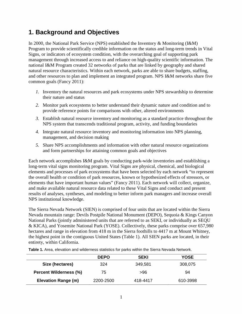
The Sierra Nevada Network (SIEN) is comprised of four units that are located within the Sierra Nevada mountain range: Devils Postpile National Monument (DEPO), Sequoia & Kings Canyon National Parks (jointly administered units that are referred to as SEKI, or individually as SEQU & KICA), and Yosemite National Park (YOSE). Collectively, these parks comprise over 657,980 hectares and range in elevation from 418 m in the Sierra foothills to 4417 m at Mount Whitney, the highest point in the contiguous United States (Table 1). All SIEN parks are located, in their entirety, within California. Table 1. Area, elevation and wilderness statistics for parks within the Sierra Nevada Network.

DEPO SEKI YOSE Size (hectares) 324 349,581 308,075

Percent Wilderness (%) 75 >96 94

Elevation Range (m) 2200-2500 418-4417 610-3998

2

The result of a 3-phase process, the SIEN Vital Signs Monitoring Plan (VSMP) describes the rationale, basis, and plan for implementing this network’s long-term ecological monitoring program (Mutch et al. 2008). The VSMP describes the collaborative process by which park staff, network staff, and numerous scientific partners from other organizations selected high priority vital signs for long-term monitoring. The top 13 vital signs ranked highest with respect to the selection criteria (significance to management, ecological importance, sensitivity to stressors, and strong linkages to other vital signs) and represented a balance of sensitive indicators that respond more quickly to stressors and more integrative indicators that respond more slowly.

Surface water dynamics and water chemistry were selected as two of the 13 high priority Vital Signs due to their widespread and significant influence on Sierra Nevada ecosystems, their resulting ecological and economic significance, and their susceptibility to anthropogenic stressors. This rivers protocol describes the importance of and our approach to hydrologic and water quality monitoring of rivers within the SIEN. Of the six protocols to be implemented, this protocol was the last to be developed. Thus, its objectives and associated operational costs were constrained by the amount of funding remaining in the program budget, and it was not feasible to develop an extensive approach to water quality and quantity monitoring with broad inferences across the network. Specific monitoring questions and objectives were determined through an iterative process with the SIEN water work group, which includes staff from SEKI and YOSE, and with input from the Resource Chiefs at SEKI and YOSE and the superintendant at DEPO (see Appendix E for a history of the protocol development). Recognizing that the SIEN Lakes Protocol (Heard et al. 2012) focuses on surface water quality at the network level the above parties decided that the limited funds for this protocol would be focused on surface water dynamics (quantity and timing) of rivers in selected major watersheds. This protocol employs a strategy that uses data from existing streamgage stations that are operated by other entities and that have historic records. We will assume operation of several gages that have been slated for abandonment by their current operators and will collaborate with park staff or other cooperators wherever possible, to ensure long-term operation of selected stations. Water chemistry objectives are limited to trend analysis of temperature data collected at existing stations and water quality data acquired from two long-term USGS Hydrologic Benchmark Network (HBN) stations. The protocol is intended to be a “living” document that will be modified as new data sources and information emerge and methodologies are refined.

1.1 Sierra Nevada Network Surface Water Monitoring Surface water dynamics in the Sierra Nevada encompasses not only streamflow, but also includes evapotranspiration, water supply to wetlands, water levels in lakes, and other components. Since comprehensive monitoring of all surface water dynamics and chemistry in the SIEN is beyond the scope and budget of our program, SIEN and park staff determined that separate protocols and objectives would be developed for lakes, wetlands, and rivers/streams. Water quality and to a lesser degree, quantity, are addressed by the Lakes Protocol (Heard et al. 2012), which uses a spatially distributed sampling design to make inferences about water quality in high-elevation lakes across the network. The Wetlands Ecological Integrity Protocol (Gage et al. In Prep) examines hydrologic regime (quantity and timing) in fens and wet meadows throughout SIEN parks, in addition to monitoring associated plant and macroinvertebrate communities. This rivers protocol focuses on water quantity and timing including changes in hydrologic regimes, and to a lesser degree, trends in water quality.

3

1.2 Rationale for Monitoring Rivers Sierra Nevada parks protect a diversity of water resources, including over 4,500 lakes and ponds, an estimated 3,450 km of mapped rivers and streams, as well as seeps, wet meadows, waterfalls, hot springs, mineral springs, and karst springs. These water resources and associated aquatic and riparian habitats have high regional ecological value, supporting aquatic communities that account for 21% of vertebrate taxa and 17% of plant taxa in the Sierra Nevada (Sierra Nevada Ecosystem Project 1996). As critical components of the larger Sierra Nevada eco-region and California’s water infrastructure, aquatic ecosystems, and hydrologic systems in the SIEN have significant economic value as they contribute to the generation of approximately $2,200,000,000 in annual revenue. Water accounts for more than 60% of these dollars (Sierra Nevada Ecosystem Project 1996). Primary water uses include irrigated agriculture, domestic water supplies, hydroelectric power, recreation, and tourism.

Rivers and streams are the primary means by which precipitation, including alpine snowpack, is delivered to ecosystems within the parks and to water users downstream of the parks. Human activities have and will continue to impact the flow regimes and water quality in SIEN rivers and streams. Such threats drive the need for expanded and continued monitoring. Science-based information about the status and trends in surface water hydrology and water quality is vital to making informed management decisions within the parks and in California. As integrators of water, energy, nutrients, solutes, and pollutants from the landscape and atmosphere, rivers are interactive components of their environment (Minshall et al. 1985). Accordingly, rivers serve as excellent sentinels of change on the surrounding landscape (Williamson et al. 2008).

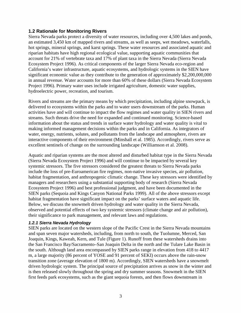
Aquatic and riparian systems are the most altered and disturbed habitat type in the Sierra Nevada (Sierra Nevada Ecosystem Project 1996) and will continue to be impacted by several key systemic stressors. The five stressors considered the greatest threats to Sierra Nevada parks include the loss of pre-Euroamerican fire regimes, non-native invasive species, air pollution, habitat fragmentation, and anthropogenic climatic change. These key stressors were identified by managers and researchers using a substantial supporting body of research (Sierra Nevada Ecosystem Project 1996) and best professional judgment, and have been documented in the SIEN parks (Sequoia and Kings Canyon National Parks 1999). All of the above stressors except habitat fragmentation have significant impact on the parks’ surface waters and aquatic life. Below, we discuss the snowmelt driven hydrology and water quality in the Sierra Nevada, observed and potential effects of two key systemic stressors (climate change and air pollution), their significance to park management, and relevant laws and regulations. 1.2.1 Sierra Nevada Hydrology SIEN parks are located on the western slope of the Pacific Crest in the Sierra Nevada mountains and span seven major watersheds, including, from north to south, the Tuolumne, Merced, San Joaquin, Kings, Kaweah, Kern, and Tule (Figure 1). Runoff from these watersheds drains into the San Francisco Bay/Sacramento–San Joaquin Delta in the north and the Tulare Lake Basin in the south. Although land area encompassed by SIEN parks range in elevation from 418 to 4417 m, a large majority (86 percent of YOSE and 91 percent of SEKI) occurs above the rain-snow transition zone (average elevation of 1800 m). Accordingly, SIEN watersheds have a snowmelt driven hydrologic system. The principal source of precipitation arrives as snow in the winter and is then released slowly throughout the spring and dry summer seasons. Snowmelt in the SIEN first feeds park ecosystems, such as the giant sequoia forests, and then flows downstream in

4

rivers and streams to serve as a primary source of water for domestic, commercial, and agricultural use throughout California.

Figure 1. Sierra Nevada Network parks and major watersheds.

5

Hydrologic data, collected from networks of snow pillows, snow courses, and streamgages are used by scientists and water managers to calculate a variety of hydrologic parameters and evaluate the quantity and timing of water delivery. Snow accumulation is measured and reported through an extensive network of snow monitoring sites (snow pillows and snow courses) by the California Department of Water Resources (CDWR). The CDWR and other water managers use data from snow courses and streamgages to develop and refine models to predict the timing and quantity of snowmelt, to develop hydrologic forecasts, and to better understand the water balance in watersheds. Because hydrology and climate are major drivers within ecosystems, observed and modeled changes in the hydrologic cycle may be used to better understand timing shifts in other ecosystem processes as well. These models need continued refinement and rely on both satellite data and manual measurements at snow courses and streamgages to contribute to the understanding of the relationship between snow cover, ablation, and streamflow.

Much of the precipitation received in a watershed, including rain and snowmelt, runs off into rivers and streams and can be measured at streamgages, which measure water level and discharge (or flow - the quantity of water, in cubic feet per second, moving past a given point on a river). A number of hydrologic parameters may be calculated from mean daily discharge data to illustrate the timing of runoff and reflect the form in which precipitation is received in watersheds. These parameters and their management relevance are listed in Table 2. Numerous studies have utilized streamflow records to document decreases in snow accumulation and earlier snowmelt (Stewart et al. 2005, Barnett et al. 2008). Because hydrology and climate are major drivers within ecosystems, these timing parameters may be used by managers to better understand timing shifts in other ecosystem processes.

6

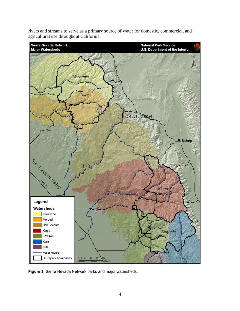
Table 2. Mountain hydrology parameters monitored by this protocol that can serve as indicators of change in runoff timing.

Hydrologic Parameter Management Significance

April-July discharge as percent of annual discharge (AMJJ/Annual)

Most of the snowmelt season occurs during the AMJJ period and these flows are the most important contribution to the annual streamflow, comprising 50-80 percent of the annual total (Stewart et al. 2005). A decrease in this value is indicative of reduced snowpack and/or a shift to more precipitation arriving as rain during other months of the year. Park ecosystems depend upon the slow release of snowmelt during the April-July period.

Onset of Snowmelt The date of the beginning of the spring prolonged snowmelt-driven streamflow. Rising temperatures may cause snowmelt to occur earlier in the year. This could lengthen the dry summer season and shift the timing of water delivery to park ecosystems.

Center of Mass This is the day of the year when half of the total annual discharge has occurred at a streamgage. The center of mass can be used as another indicator of snowmelt timing.

Number of Days to the 3-day high flow

This is the number of days from October 1 to the highest consecutive 3-day discharge of the water year. Typically, the 3-day high flow occurs during the peak snowmelt runoff period, whereas the single day peak flow could result from a rainstorm. Similar to the center of mass and snowmelt onset, earlier 3-day high flows can indicate an earlier melt due to rising temperatures. Trends in earlier 3-day high flows in the SIEN were observed by Andrews (2012).

Winter low flows (3, 7, 10 or 14-day low flow)

The smallest value observed over 3, 7, 10 or 14 consecutive days. An increase in the volume of winter low flows would indicate that more precipitation is arriving in the form of rain during the winter months. The total volume of precipitation (and total annual discharge) may remain the same while the timing and form (rain vs. snow) may change. Park ecosystems would need to adapt to such shifts.

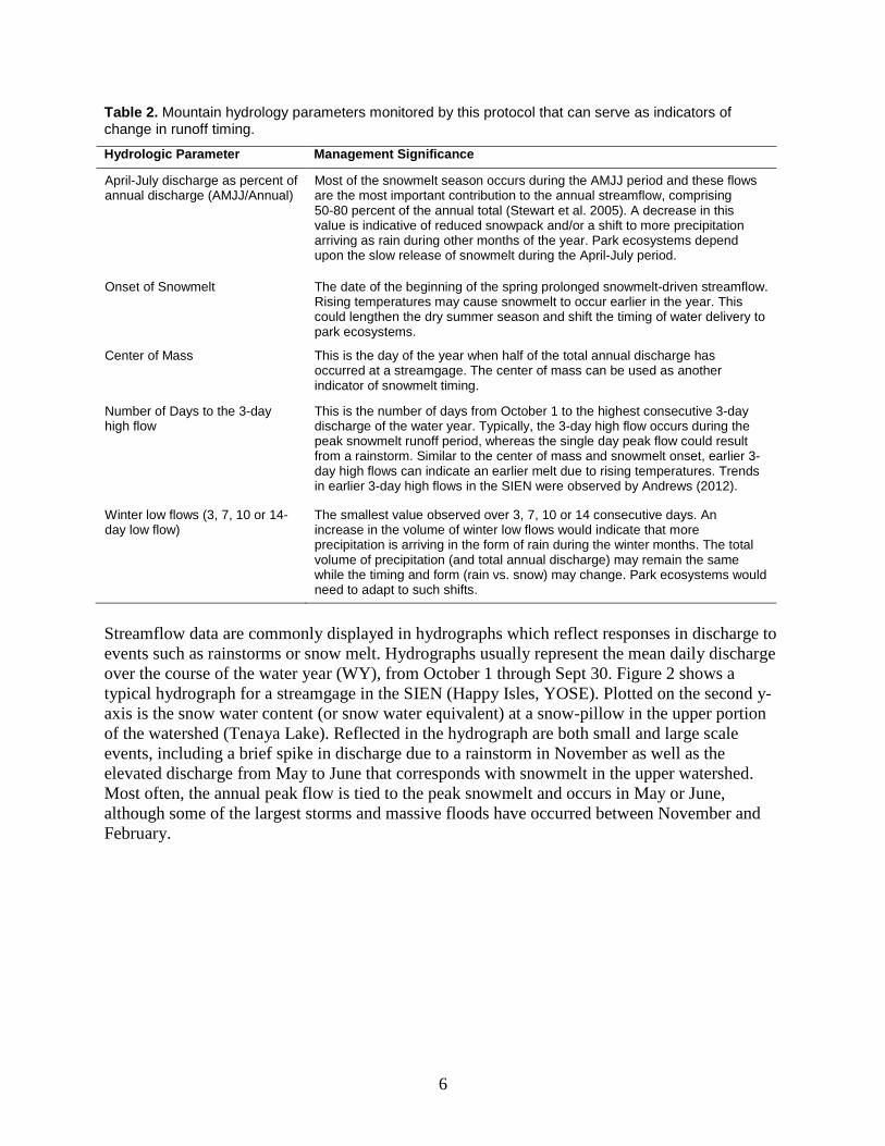
Streamflow data are commonly displayed in hydrographs which reflect responses in discharge to events such as rainstorms or snow melt. Hydrographs usually represent the mean daily discharge over the course of the water year (WY), from October 1 through Sept 30. Figure 2 shows a typical hydrograph for a streamgage in the SIEN (Happy Isles, YOSE). Plotted on the second y-axis is the snow water content (or snow water equivalent) at a snow-pillow in the upper portion of the watershed (Tenaya Lake). Reflected in the hydrograph are both small and large scale events, including a brief spike in discharge due to a rainstorm in November as well as the elevated discharge from May to June that corresponds with snowmelt in the upper watershed. Most often, the annual peak flow is tied to the peak snowmelt and occurs in May or June, although some of the largest storms and massive floods have occurred between November and February.

7

Figure 2. An example of the relationship between snow accumulation and snowmelt at the Tenaya Lake snowcourse in the upper Merced Watershed and discharge at the Happy Isles streamgage in the lower portion of the watershed. Note the dramatic increase in discharge (blue solid line) as snowpack rapidly melts (green solid line) in early May.

In the coming decades, climate change and variability will undoubtedly have profound effects on water resources in the Sierra Nevada and the ecosystems that have evolved within a snowmelt-driven hydrologic system. Changes have already been observed and are expected to continue (Knowles et al. 2006, Null et al. 2010, Intergovernmental Panel on Climate Change 2007). Barnett et al. (2008) predict a coming water crisis in the western United States, and their results show that “up to 60% of the climate-related trends of river flow, winter air temperature, and snow pack between 1950 and 1999 are human-induced”. The conceptual model in Figure 3 illustrates the ecological mechanisms and feedback loops by which climate change may affect streamflow.

One of the most widely observed trends that will continue to have profound effects on the hydrologic cycle has been an increase in surface air temperatures; the Sierra Nevada has warmed 0.5 to 1.5 oC over the last 50 years (Mote et al. 2005). In the western US, some of the most notable effects of increased air temperatures on river dynamics occur through the effects of air temperature on snow accumulation and snow melt. Air temperature influences the form in which precipitation falls, and warmer air temperatures raise the elevation of the rain-snow transition zone. In the mountains, as this zone moves upward, more precipitation falls as rain rather than snow. Although increased snowpack has been observed (data from 1950-1997) at higher elevations in the Sierra Nevada (Mote et al. 2005, Andrews 2012), Stewart (2009) states that “with continued warming, increasingly higher elevations are projected to experience declines in snowpack accumulation and melt that can no longer be offset by winter precipitation increases”.

8

Figure 3. Conceptual model of ecological mechanisms and feedbacks by which climate change can affect streamflow in snow dominated watersheds (from Tague and Dugger 2010).

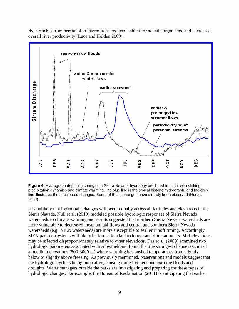
Researchers have documented hydrologic changes (earlier snowmelt runoff, reduced summer base flows, and decreased winter snowpack) in the Sierra Nevada and western US and predict further changes (Stewart et al. 2005, Mote et al. 2005). These changes and others, including wetter and more erratic winter flows, prolonged low summer flows, reduced soil moisture, and periodic drying of once perennial streams are depicted in the hydrograph in Figure 4. In the Sierra Nevada, annual precipitation, and consequently annual streamflow, are highly variable, commonly more so than in other parts of the US. Additionally, it is not uncommon for most of the annual water to be delivered in just a few large snow or rain storms each year (Dettinger et al. 2011). Throughout the SIEN and much of California, some of the largest floods have occurred during winter rainstorms. This type of storm caused the floods that closed Yosemite Valley in Yosemite National Park in January 1997 and May 2005. Floods can be magnified in the winter when high-altitude rains in the Sierra Nevada either melt or run off of an existing snowpack. Predictions for even greater variability in precipitation and streamflow along with more extreme events pose a dilemma for park managers and California water managers who may no longer be able to depend on the historic hydrologic system in which the majority of the precipitation for the year arrives and is stored as snow to be released throughout the summer. Greater variability in precipitation and less total snowfall could result in reduced summer low flows, the transition of

9

river reaches from perennial to intermittent, reduced habitat for aquatic organisms, and decreased overall river productivity (Luce and Holden 2009).

Figure 4. Hydrograph depicting changes in Sierra Nevada hydrology predicted to occur with shifting precipitation dynamics and climate warming.The blue line is the typical historic hydrograph, and the grey line illustrates the anticipated changes. Some of these changes have already been observed (Herbst 2008).

It is unlikely that hydrologic changes will occur equally across all latitudes and elevations in the Sierra Nevada. Null et al. (2010) modeled possible hydrologic responses of Sierra Nevada watersheds to climate warming and results suggested that northern Sierra Nevada watersheds are more vulnerable to decreased mean annual flows and central and southern Sierra Nevada watersheds (e.g., SIEN watersheds) are more susceptible to earlier runoff timing. Accordingly, SIEN park ecosystems will likely be forced to adapt to longer and drier summers. Mid-elevations may be affected disproportionately relative to other elevations. Das et al. (2009) examined two hydrologic parameters associated with snowmelt and found that the strongest changes occurred at medium elevations (500-3000 m) where warming has pushed temperatures from slightly below to slightly above freezing. As previously mentioned, observations and models suggest that the hydrologic cycle is being intensified, causing more frequent and extreme floods and droughts. Water managers outside the parks are investigating and preparing for these types of hydrologic changes. For example, the Bureau of Reclamation (2011) is anticipating that earlier

10

snowmelt and more rain resulting from warmer conditions may reduce their current infrastructure’s ability to provide effective flood protection. To inform planning and management decisions, long-term data are crucial. Hannaford et al. (2011) noted “there is a growing need for observational data with which to discern any emerging trends in river flows and to compare these with future projections from climate models”. Despite the importance of and need for hydrologic data within SIEN parks, the amount and availability of relevant data has been declining. Historically, hydrologic data in and near the parks have primarily been collected by researchers or agencies other than the NPS. Recognizing the need for hydrologic data to inform the state’s water management system and flood prediction efforts, USGS and other agencies operated more than 30 streamgages in or within 20 miles of SIEN parks in the 1980s and 90s. Since then, over half of these stations have been abandoned by their operators, primarily due to funding cuts. Furthermore, streamgages are commonly installed by an agency or researcher with their specific research or program needs in mind, and their data are not widely shared. Parks often do not have the time, staff, or resources to seek out and acquire data from disparate sources, and consolidate and analyze these data sets for trends in hydrologic parameters relevant to park management. This protocol will assist with the collection, management, and analysis of such data.

The SIEN I&M Program provides valuable information about the status and trends of natural resources through long-term monitoring so that the parks may fully integrate natural resource monitoring and other science activities into the management processes of the National Park System, as laid out in the National Parks Omnibus Management Act (NPS 1998). The Act charges the Secretary of the Interior to "continually improve the ability of the National Park Service to provide state-of-the-art management, protection, and interpretation of and research on the resources of the National Park System". Park managers rely upon monitoring results to prioritize protection or restoration efforts and for scenario planning. Further, the Interagency Climate Change Adaptation Task Force (2011) has developed a national action plan to identify steps that federal agencies can take to improve management of freshwater resources in a changing climate and with the following national goal:

Government agencies and citizens collaboratively manage freshwater resources in response to a changing climate in order to assure adequate water supplies, to protect human life, health and property, and to protect water quality and aquatic ecosystems.

The action plan recognizes that although many of the policies and decision making tools used by resource managers rely on historic data, in a changing climate, complete and current data must be used along with predictive models that use current data. With this protocol, the SIEN will provide routine summaries of surface water status and trends to the parks and make the data available for use in predictive models that can provide valuable information for planning and management decisions.

1.2.2 Sierra Nevada Surface Water Quality SIEN surface waters are judged to be of excellent quality by state and federal water quality standards. There are few aquatic areas outside the parks that have not been impacted by diversions or other activities such as mining; thus SIEN stream reaches have been selected as reference conditions for monitoring programs such as the state’s Surface Water Ambient

11

Monitoring Program (see Appendix 1 for more information). Climate change and air pollution are among the largest threats to water quality in the Sierra Nevada. Rising air temperature and changes in the hydrologic cycle associated with climate change will have impacts on aquatic systems and water quality. Kaushal et al. (2010) examined water temperatures in rivers and streams throughout the US and found long-term water temperature warming at half of the sites; these increases were well correlated with air temperature increases. Coupled with the expected periodic drying of once perennial reaches due to shifts in the hydrologic cycle, increased water temperature is likely to have adverse effects on aquatic life and may alter community biodiversity.

For the most part, surface waters in the SIEN are very dilute which makes them particularly sensitive to anthropogenic disturbances (Clow et al. 1996). The western slope of the central and southern Sierra Nevada is impacted by some of the worst air pollution in the United States (Cahill et al. 1996). Contaminants and nutrients, produced from agricultural, urban, and industrial sources in the San Francisco Bay Area and the Central Valley are transported by air currents into the Sierra Nevada where they are deposited as wet or dry deposition.

Preparing for such changes and protecting park resources from external non-point sources is challenging for park management. Despite similar challenges, Rocky Mountain National Park has developed a resource management goal for nitrogen deposition. Collaboratively, the Colorado Department of Public Health and Environment, the U.S. Environmental Protection Agency Region 8 (EPA), and the National Park Service developed a Nitrogen Deposition Reduction Plan (Baker et al. 2007). Data from research and monitoring in the park were used to identify critical loads for nitrogen deposition. Although compliance is voluntary, this is seen as an important step in protecting parks from excessive nitrogen inputs. The California State Water Resources Control Board is undertaking similar investigations in preparation for a nutrient policy that would establish nutrient water quality objectives and establish methods to control nutrient over-enrichment in inland surface waters of the state (State Water Resources Control Board 2011). Parks can use information about trends in surface water nutrients to influence state and national policy decisions. To provide management with relevant information about water quality trends, we will monitor water temperature continuously (at 15-minute intervals) at streamgages where it is feasible. Additionally, we will acquire and analyze water quality data, including nutrients, from the two long-term Hydrologic Benchmark Network stations in the SIEN.

1.3 Thresholds and Guidelines for Management 1.3.1 State and federal standards and guidance The State Water Resources Control Board and nine Regional Water Quality Control Boards (RWQCB), under the Porter-Cologne Water Quality Control Act (1969), are responsible for the protection and enhancement of California’s water resources. Each RWQCB adopts one or more Basin Plans, which contain beneficial use designations, water quality objectives, and implementation programs. Sierra Nevada Network parks fall under the jurisdiction of the Central Valley RWQCB and have waters contained in both the Sacramento–San Joaquin Delta and Tulare Lake Basins.

Pursuant to the federal Clean Water Act (1972), water quality standards comprise two parts: 1) designated uses—referred to as beneficial uses by the State of California, and 2) water quality criteria to protect those uses—or under California Water Code, water quality objectives. The RWQCB designates beneficial uses for specified river segments or waterbodies within the major

12

river basins: Tuolumne, Merced, San Joaquin, Kings, Kaweah, Tule, and Kern (Table 3). Water quality objectives are adopted by the RWQCB, can be applied to any surface waters, and are defined as "...the limits or levels of water quality constituents or characteristics which are established for the reasonable protection of beneficial uses of water or the prevention of nuisance within a specific area" [Water Code Section 13050(h)]. Objectives for SIEN waters may be found in the Basin Plan for the Central Valley Region (Bruns 1998). There are presently no water quality objectives for the majority of the water chemistry constituents monitored in this protocol. However, nutrients are among the constituents monitored in the SIEN and the California Water Quality Control Board is proposing a nutrient policy that would establish nutrient water quality objectives and establish methods to control nutrient over-enrichment in inland surface waters of the state.

Under sections 305(b) and 303(d) of the Clean Water Act, California is required to assess the overall health of the State’s waters and identify waters that are not attaining water quality standards. The State must compile water quality impaired waters in a 303(d) list and initiate the process to bring listed waters back into compliance. Sierra Nevada Network parks do not contain any 303(d) listed waters (State Water Resources Control Board 2002). The State also has the authority to designate waters as Outstanding Natural Resource Waters. This designation affords the highest level of protection, under the Clean Water Act. At present, Sierra Nevada Network parks do not have any Outstanding Natural Resource Waters; however, national park waters are strong candidates for this designation.

Portions of six of the seven major rivers in the SIEN have been designated or determined to be eligible for wild and scenic rivers designation. The designation includes identification of the rivers’ Outstandingly Remarkable Values (ORVs), river-related values that make a river unique and worthy of special protection. These values include aesthetic, recreational, biological, and hydrological features. The Wild and Scenic Rivers Act requires protection of ORVs along designated reaches. In addition, no actions may be taken that could adversely affect the values that qualify a river for the national wild and scenic rivers system, thus extending protection to rivers eligible for designation. Long-term hydrologic and water chemistry monitoring on these rivers will inform the parks understanding of the status and trends and guide management decisions needed to protect the ORVs.

1.3.2 SEKI-specific thresholds In SEKI, Southern California Edison (SCE) has diverted water from the Middle and Marble Forks of the Kaweah River for power generation since 1907. An analysis was completed in 1980 (Jordan / Avent & Associates 1984) to determine the effects of the SCE diversions and to ensure that the minimum flow requirements laid out in the park-mandated special use permit were adequate to support healthy aquatic ecosystems downstream of the diversions. The report found that the diversions were not causing undue impacts, and the renewed special use permit established new minimum flow requirements. SCE operates multiple gages and reports the data to the park superintendant, as required by their special use permit, to ensure that they are maintaining the minimum flow requirements in the Kaweah. SCE also provides their streamflow data to SIEN for analysis and reporting. We will examine the records and report any failures to comply with the minimum flow requirements, which are described in SOP 9.

13

Table 3. Beneficial uses for SIEN waterbodies (California Regional Water Quality Control Board Central Valley Region 1995, 1998).

Beneficial Uses Park Watershed Stream Segment MUN AGR POW REC1 REC2 WARM COLD WILD RARE SPWN FRSH

DEPO San Joaquin Sources to Millerton Lake X X X X X X X X

SEKI San Joaquin Sources to Millerton Lake X X X X X X X X

Kings Main Fork, Above Kirch Flat X X X X X X X X X

Kaweah Above Lake Kaweah X X X X X X X X X X

Tule Above Lake Success X X X X X X X X X X X

Kern Above Lake Isabella X X X X X X X X X X

YOSE Merced Source to McClure Lake X X X X X X X

Tuolumne Source to (new) Don Pedro X X X X X X X X

MUN: Municipal and domestic supply AGR: Agricultural supply POW: Hydropower generation REC1: Water contact recreation REC2: Non-contact water recreation WARM: Warm freshwater habitat COLD: Cold freshwater habitat WILD: Wildlife habitat RARE: Rare, threatened, or endangered species SPWN: Spawning, reproduction, and/or early development FRSH: Freshwater replenishment

14

1.4 Monitoring Questions and Measurable Objectives 1.4.1 Monitoring Questions As part of the Vital Signs selection process, park and network staff, and outside cooperators identified and prioritized resource-related questions of interest. As mentioned earlier, surface water dynamics and chemistry encompass a broad range of topics, and are monitored through this rivers protocol as well as the Lakes Protocol and Wetlands Integrity protocols. Questions of interest identified in the Vital Signs Monitoring Plan with relevance to rivers include:

Surface water dynamics 1. How are climatic trends affecting regional hydrologic regimes (snowpack depth, snow water

equivalent, snowmelt, glacial extent, frequency and intensity of flood events and volume and timing of river and stream flows)?

2. How are stream and river discharge rates and the timing and magnitude of peak flows changing?

3. How are water dynamics changing in response to climate change and fire regimes?

Water quality questions 4. How does water chemistry (concentrations and fluxes) vary temporally across network

parks? 5. How is surface water quality changing with respect to state and national water quality

standards?

1.4.2 Primary Measureable Objectives The focus of this protocol is primarily the timing and quantity of streamflow and secondarily on water chemistry. Our approach towards achieving these protocol objectives is to acquire data from existing stations with long periods of record, to compile, analyze, and report on these data, and to assume or support operation of a few selected stations over time, if and when the original operators are no longer able.

1) Detect long term trends in timing and volume of streamflow using fixed, continuous, water stage recording stations at existing streamgages in selected major watersheds of the SIEN. The SIEN will record, measure and/or calculate the hydrologic measures listed below for each selected streamgage:

a. Stage b. Discharge – Instantaneous (measured), mean annual, instantaneous peak, and highest

and lowest daily mean c. Number of days to center of mass and onset of snowmelt d. Winter and summer 3, 7, 10 and 14-day low and high flow e. Number of days to winter and summer 7-day low flow f. Number of days to 3 and 14-day high flow g. Percent AMJJ/Annual flow.

15

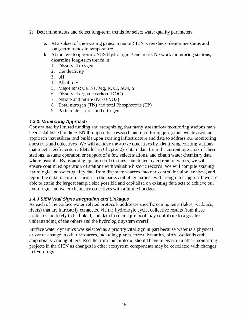
2) Determine status and detect long-term trends for select water quality parameters:

a. At a subset of the existing gages in major SIEN watersheds, determine status and long-term trends in temperature

b. At the two long-term USGS Hydrologic Benchmark Network monitoring stations, determine long-term trends in: 1. Dissolved oxygen 2. Conductivity 3. pH 4. Alkalinity 5. Major ions: Ca, Na, Mg, K, Cl, SO4, Si 6. Dissolved organic carbon (DOC) 7. Nitrate and nitrite (NO3+NO2) 8. Total nitrogen (TN) and total Phosphorous (TP) 9. Particulate carbon and nitrogen

1.3.3. Monitoring Approach Constrained by limited funding and recognizing that many streamflow monitoring stations have been established in the SIEN through other research and monitoring programs, we devised an approach that utilizes and builds upon existing infrastructure and data to address our monitoring questions and objectives. We will achieve the above objectives by identifying existing stations that meet specific criteria (detailed in Chapter 2), obtain data from the current operators of these stations, assume operation or support of a few select stations, and obtain water chemistry data where feasible. By assuming operation of stations abandoned by current operators, we will ensure continued operation of stations with valuable historic records. We will compile existing hydrologic and water quality data from disparate sources into one central location, analyze, and report the data in a useful format to the parks and other audiences. Through this approach we are able to attain the largest sample size possible and capitalize on existing data sets to achieve our hydrologic and water chemistry objectives with a limited budget.

1.4.3 SIEN Vital Signs Integration and Linkages As each of the surface water-related protocols addresses specific components (lakes, wetlands, rivers) that are intricately connected via the hydrologic cycle, collective results from these protocols are likely to be linked, and data from one protocol may contribute to a greater understanding of the others and the hydrologic system overall.

Surface water dynamics was selected as a priority vital sign in part because water is a physical driver of change in other resources, including plants, forest dynamics, birds, wetlands and amphibians, among others. Results from this protocol should have relevance to other monitoring projects in the SIEN as changes in other ecosystem components may be correlated with changes in hydrology.

16

1.5 Major Watersheds of the Sierra Nevada Network Below is a brief overview of each of the major watersheds in the SIEN, including monitoring stations selected for this protocol. Appendix A of this protocol provides a summary of relevant surface water research and monitoring projects taking place in SIEN watersheds. In-depth summaries of SIEN water resources information may be found in Heard and Stednick (2005) and Boiano et al. (2005). More information about the stations selected for this protocol can be found in Chapter 2 as well as SOP 1.

1.5.1 Yosemite National Park Yosemite National Park contains the headwaters and significant portions of the Tuolumne and Merced watersheds. Portions of both rivers have been designated as wild and scenic rivers and river management plans are in development by YOSE. Both the Tuolumne and Merced watersheds have been the subject of intensive collaborative research as part of the Yosemite Hydroclimate Project from the late 1990s to present. The project involved researchers from a number of universities and governmental organizations who undertook studies to better understand hydrology and climate in the park (Lundquist et al. 2003). A number of the studies paired meteorological stations with streamgages to better understand precipitation contributions, special dynamics and intra-annual variation (Peterson et al. 2005).

Eight of the fourteen stations included in this protocol are located in YOSE. Two of the stations, the Merced near High Sierra Camp and the Lyell Fork of the Tuolumne, were installed by USGS researcher Dave Clow in 2001 as part of the Hydroclimate Project. Although other projects are on-going, Clow’s research and operation of the stations has ended. Pending evaluation of the rating curves and historic data, the SIEN and YOSE will cooperatively continue operation of the stations.

The headwaters of the Merced River watershed originate on the slopes of Mount Lyell and the Clark Range of the Sierra Nevada. The main stem flows through Little Yosemite Valley, past Half Dome, over Nevada and Vernal Falls and into the Yosemite Valley, the most heavily developed area of the park. The South Fork runs through the southern portion of the park and leaves the park near Wawona, the park’s south entrance. All of the famous waterfalls in Yosemite Valley meet the main stem of the Merced River on the Valley floor.

The Merced River Watershed

A large portion of the hydrologic and water quality monitoring in the watershed has been conducted by the USGS. The hydrology of the Merced River watershed is of high interest to a number of downstream water users such as the Merced Irrigation District (MID) which utilizes the water for both hydroelectric power and irrigation.

Four of the stations selected for this protocol are located in the greater Merced Watershed, three on the main stem and one on the South Fork (Figure 5). The USGS California Water Science Center operates two of the stations, located on the section of the Merced within Yosemite Valley. Sierra Hydrographics (a consulting company contracted by MID) operates the station on the South Fork Merced. The other station was formerly operated by USGS researcher Dave Clow (out of the Colorado Water Science Center). We have identified this station for possible long-term operation by SIEN.

17

The streamflow records at the Merced River Yosemite Valley stations are among the longest in the nation, beginning in 1915 at the Happy Isles streamgage and in 1916 at Pohono Bridge. These long-term records are valuable to and widely used by researchers and water managers throughout California to understand and predict changes in climate, flood prediction, park planning, and to assess the availability and quality of water supplies.

The Happy Isles gage has a corresponding long-term water quality monitoring record (1967-present), collected through the Hydrologic Benchmark Network (HBN), a long-term monitoring program of the USGS. The HBN is designed to study status and trends in surface water chemistry in minimally affected basins and as a benchmark against which to compare changes in developed watersheds. The USGS performed an analysis of the water quality data in 2000 (Mast and Clow 2000), however frequent trend analyses are not a part of the long-term monitoring plan for these stations. Consequently, the SIEN will periodically analyze and report on water quality trends from this station.

The headwaters of the Tuolumne River, the Dana and Lyell Forks, arise on the slopes of Mount Dana near Tioga Pass at the base of the Lyell and Maclure glaciers, the largest glaciers remaining on the west slope of the Sierra Nevada. The Dana and Lyell Forks converge at Tuolumne Meadows to form the main stem which continues for 27 miles before ultimately flowing into 8-mile long Hetch Hetchy reservoir, which is the primary water source to the City of San Francisco.

The Tuolumne River Watershed

Four of the stations selected for this protocol are located in the greater Tuolumne River watershed (Figure 6). Hetch Hetchy Water and Power (HHWP), which has a strong interest in understanding and predicting hydrologic dynamics in the watershed, funds the Tuolumne above Hetch Hetchy and operates a stations on Falls Creek, which flows into the reservoir. HHWP may also collaborate with YOSE and SIEN on a third station, the Tuolumne at Tioga Road Bridge, which is currently operated by YOSE, California Department of Water Resources, and several academic researchers. We have identified another station, installed and formerly operated as part of a research project by Dave Clow (USGS), for potential long-term operation by SIEN. The station, located on the upper portion of the Lyell Fork of the Tuolumne at 9615 ft, is the highest elevation station selected for this protocol. Hydrologic and climate data from high elevations in the Sierra Nevada is sparse, but needed. In conjunction with stations at lower elevations, these data are particularly valuable for understanding the hydrology in contributing headwater basins and for investigating whether streamflow trends vary across an elevational gradient.

18

Figure 5. The Greater Merced Watershed, monitoring stations included in this protocol, and station operators.

19

Figure 6. The Greater Tuolumne Watershed, monitoring stations included in this protocol, and station operators.

20

1.5.2 Devils Postpile National Monument

Approximately 3.5 miles of the Middle Fork of the San Joaquin River is within DEPO, and includes one waterfall, Rainbow Falls, that is a popular attraction for visitors. Multiple segments of the river within and adjacent to DEPO have been classified as eligible for designation as a Wild and Scenic River. In 2009, DEPO cooperated with the USGS to install a streamgage on the river near the northern boundary of the park (

The Middle Fork of the San Joaquin River Watershed

Figure 7, See SOP 1 for a more detailed map). DEPO and SIEN will jointly fund USGS operation of the station. Prior to the installation, hydrologic monitoring was limited to water level, which was collected as part of the Soda Spring Meadow meteorological station that is operated by Scripps Institution of Oceanography and the California Department of Water Resources. In conjunction with the meteorological station, the streamgage provides valuable long-term information about hydrologic dynamics in DEPO, the Middle Fork of the San Joaquin, and the eastern side of SIEN. This data can be used by DEPO for scenario planning and to better understand dynamics in other resources such as meadows.

DEPO staff conduct monthly water quality monitoring at three locations on the San Joaquin River as well as two tributaries. Water quality monitoring visits include discharge measurements when possible. These data are stored in an NPStoret database at DEPO.

21

Figure 7. The Middle Fork of the San Joaquin Watershed including the Devils Postpile streamgage.

22

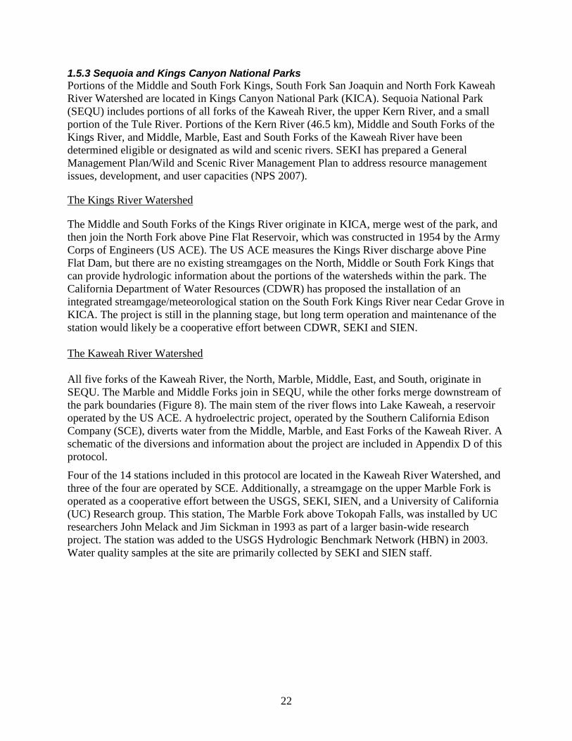
1.5.3 Sequoia and Kings Canyon National Parks Portions of the Middle and South Fork Kings, South Fork San Joaquin and North Fork Kaweah River Watershed are located in Kings Canyon National Park (KICA). Sequoia National Park (SEQU) includes portions of all forks of the Kaweah River, the upper Kern River, and a small portion of the Tule River. Portions of the Kern River (46.5 km), Middle and South Forks of the Kings River, and Middle, Marble, East and South Forks of the Kaweah River have been determined eligible or designated as wild and scenic rivers. SEKI has prepared a General Management Plan/Wild and Scenic River Management Plan to address resource management issues, development, and user capacities (NPS 2007).

The Middle and South Forks of the Kings River originate in KICA, merge west of the park, and then join the North Fork above Pine Flat Reservoir, which was constructed in 1954 by the Army Corps of Engineers (US ACE). The US ACE measures the Kings River discharge above Pine Flat Dam, but there are no existing streamgages on the North, Middle or South Fork Kings that can provide hydrologic information about the portions of the watersheds within the park. The California Department of Water Resources (CDWR) has proposed the installation of an integrated streamgage/meteorological station on the South Fork Kings River near Cedar Grove in KICA. The project is still in the planning stage, but long term operation and maintenance of the station would likely be a cooperative effort between CDWR, SEKI and SIEN.

The Kings River Watershed

The Kaweah River Watershed All five forks of the Kaweah River, the North, Marble, Middle, East, and South, originate in SEQU. The Marble and Middle Forks join in SEQU, while the other forks merge downstream of the park boundaries (Figure 8). The main stem of the river flows into Lake Kaweah, a reservoir operated by the US ACE. A hydroelectric project, operated by the Southern California Edison Company (SCE), diverts water from the Middle, Marble, and East Forks of the Kaweah River. A schematic of the diversions and information about the project are included in Appendix D of this protocol.

Four of the 14 stations included in this protocol are located in the Kaweah River Watershed, and three of the four are operated by SCE. Additionally, a streamgage on the upper Marble Fork is operated as a cooperative effort between the USGS, SEKI, SIEN, and a University of California (UC) Research group. This station, The Marble Fork above Tokopah Falls, was installed by UC researchers John Melack and Jim Sickman in 1993 as part of a larger basin-wide research project. The station was added to the USGS Hydrologic Benchmark Network (HBN) in 2003. Water quality samples at the site are primarily collected by SEKI and SIEN staff.

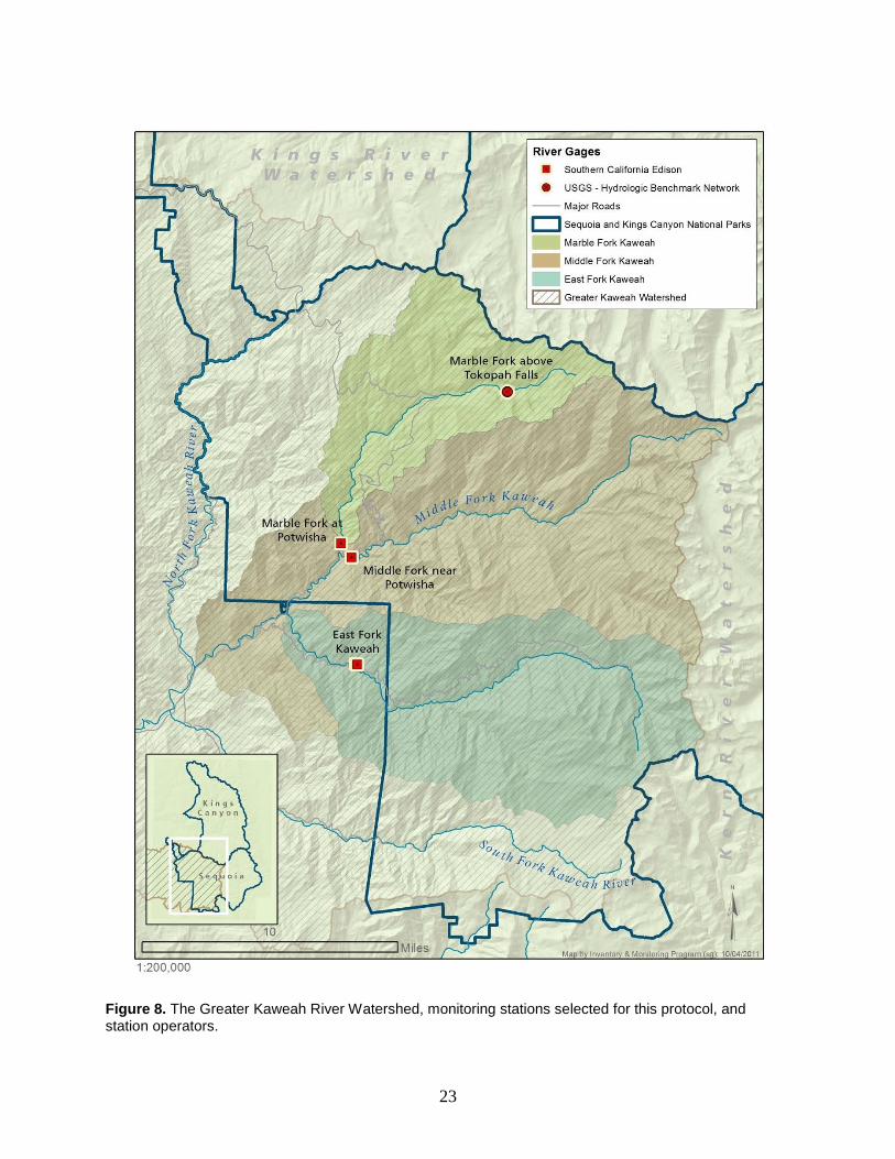
23

Figure 8. The Greater Kaweah River Watershed, monitoring stations selected for this protocol, and station operators.

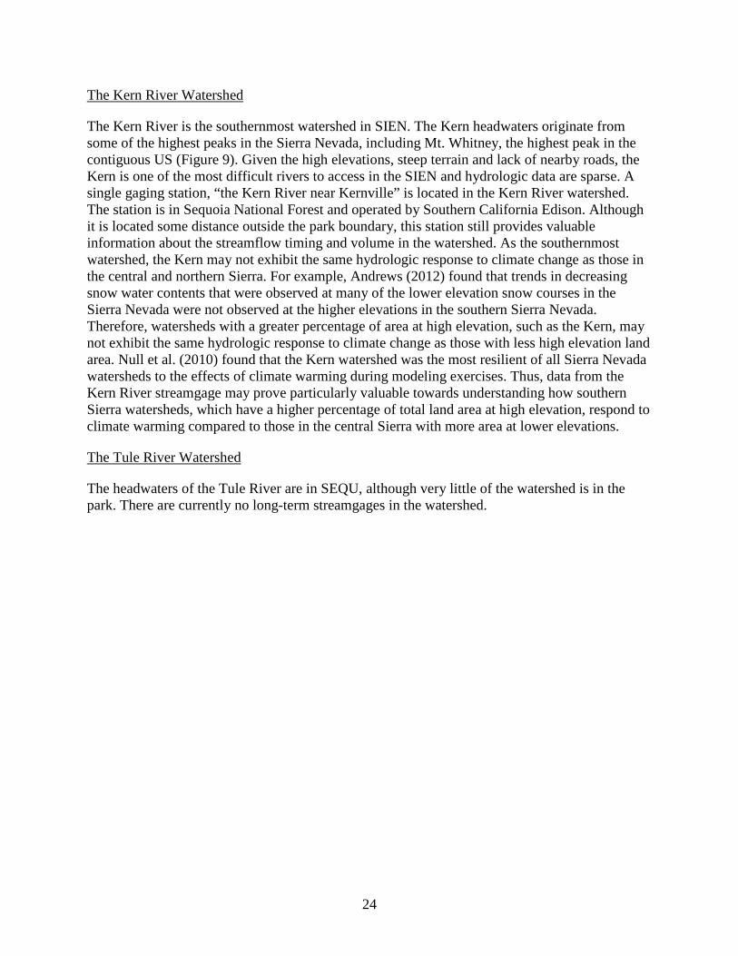
24

The Kern River is the southernmost watershed in SIEN. The Kern headwaters originate from some of the highest peaks in the Sierra Nevada, including Mt. Whitney, the highest peak in the contiguous US (

The Kern River Watershed

Figure 9). Given the high elevations, steep terrain and lack of nearby roads, the Kern is one of the most difficult rivers to access in the SIEN and hydrologic data are sparse. A single gaging station, “the Kern River near Kernville” is located in the Kern River watershed. The station is in Sequoia National Forest and operated by Southern California Edison. Although it is located some distance outside the park boundary, this station still provides valuable information about the streamflow timing and volume in the watershed. As the southernmost watershed, the Kern may not exhibit the same hydrologic response to climate change as those in the central and northern Sierra. For example, Andrews (2012) found that trends in decreasing snow water contents that were observed at many of the lower elevation snow courses in the Sierra Nevada were not observed at the higher elevations in the southern Sierra Nevada. Therefore, watersheds with a greater percentage of area at high elevation, such as the Kern, may not exhibit the same hydrologic response to climate change as those with less high elevation land area. Null et al. (2010) found that the Kern watershed was the most resilient of all Sierra Nevada watersheds to the effects of climate warming during modeling exercises. Thus, data from the Kern River streamgage may prove particularly valuable towards understanding how southern Sierra watersheds, which have a higher percentage of total land area at high elevation, respond to climate warming compared to those in the central Sierra with more area at lower elevations.

The headwaters of the Tule River are in SEQU, although very little of the watershed is in the park. There are currently no long-term streamgages in the watershed.

The Tule River Watershed

25

Figure 9. The Kern River Watershed and Kern River streamgage.

27

2. Sampling Design Monitoring-related sampling designs typically fall into three broad categories: census, probabilistic, and judgment. Census monitoring designs sample all units within a target population (e.g., all lakes within a park) and are rare due to the level of sampling effort and costs involved. The use of probabilistic designs has increased in recent years among natural resource monitoring programs because they ensure that the sample unit represents a random subsample of the target population, thus allowing inference from subsample to the target population. The judgment sample design focuses on specific sample units that are selected based on expert judgment or specific selection criteria.

Water resource monitoring programs commonly use more than one design depending on the management question being asked. Judgmental sampling is a common monitoring design for surface water monitoring among state, federal and citizen monitoring programs, is recommended by the EPA (1997), and is used by the USGS National Water Quality Assessment Program and the Washington State streamflow monitoring program (Butkus 2005). Judgmental sampling is commonly used for hydrologic monitoring because it is difficult to obtain suitable stream reaches using a random selection process. Rather, locations typically are selected using the best professional judgment to ensure that a site is representative of a particular sub-watershed and has specific characteristics, such as stream bank and channel characteristics that are stable over time, stream size and slope that are conducive to discharge measurements, and easy access. Probabilistic sampling would be extremely difficult to implement because the design would likely select numerous sites that do not have the specific characteristics suitable for a streamgage. The limitation of the judgment sample design is that data cannot be used to make inference beyond the individual streamgage locations.

2.1 Monitoring Approach The focus of this protocol is primarily the timing and quantity of streamflow and secondarily water chemistry. The desired target population is rivers in mid to large size watersheds in the SIEN parks. We have chosen to use a judgmental sample design that relies on existing stations because 1) a probabilistic sampling design to establish new streamgage locations is not logistically or financially feasible and 2) the use of existing streamgage locations allows us to take advantage of and build upon historic records. Hydrologic measures commonly have high variability and signal to noise ratio compared to many other ecological indicators, which makes long-term records especially valuable for trend analyses. We will compile, analyze, and report on data from selected existing stations and may assume operation of several stations if their current operators are no longer able.

The advantages of using existing streamgages are that locations have already been expertly selected, equipment has already been purchased and installed, rating curves that describe the stage/discharge relationship have been developed, and historic data are available. We initially considered the possibility of installing new stations in areas that are not well represented or re-installing stations that had been removed. However, it was not possible to find stations that met all of our selection criteria (see section 2.2 below) and fit within our budget and staffing plan. Installation of new stations would have been expensive and time-consuming because the development of rating curves requires frequent visits in the initial years (i.e., up to 10 years) in order to obtain discharge measurements over a wide range of streamflows. After the initial years

28

of operation and if a relatively stable reach has been selected, the stage/discharge relationship will not change much, and only periodic discharge measurements are required to check for shifts in the rating curve. By selecting existing stations, we are able to achieve greater efficiency with our time and budget because we are able to build upon existing rating curves and make fewer station visits. Further, when performing trend analyses, most hydrologists prefer stream discharge records that exceed 30 years so that decadal oscillations in precipitation (averages about 11 years) can be incorporated in the analyses. The incorporation of existing stations into our sampling design allows us to examine some records for trends immediately and other records significantly sooner than if we were installing new stations. By adopting this sampling design we are not able to represent all watersheds of interest and will not be able to make statistical inference to all watersheds across the network. Our analyses and conclusions will be largely catchment-specific. Our network of stations provides information about the timing and quantity of precipitation received in the watershed upstream of each station and may serve as sentinels of change across the SIEN. However, Andrews (2012) found excellent coherence with mean annual discharge between stations in mid-sized watersheds throughout the SIEN, even those separated by considerable distance and on opposite sides of the Sierras. We feel that if similar trends are observed, such as an earlier snowmelt onset at a number of stations throughout the network, such findings would be significant for management consideration and may indicate areas for further investigation through modeling or targeted research.

Within the Tuolumne, Merced, and Marble Fork Kaweah watersheds, we have the opportunity to explore hydrologic relationships within the context of “nested watersheds”. The agencies that installed and operate existing gages in these watersheds selected station locations based on a nested watershed approach. A nested watershed approach involves selecting multiple stations within a watershed whereby there are multiple smaller or “sub-watersheds” within the larger. Stations that occur farther downstream and at lower elevations have progressively larger contributing areas. Here ‘sub-watershed’ refers to the area that contributes runoff to the streamgage rather than the typical definition where a sub-watershed is delineated at the point where a smaller stream joins a larger one. Thus, the contributing area and hydrology of each streamgage can be examined within the context of the next larger (or smaller) watershed. Ecosystems often show non-linear responses along altitudinal gradients to changes in environmental parameters, such as temperature (Becker et al. 1997). This may be particularly relevant in the Sierra Nevada where the greatest response to a warming climate is likely to be seen at mid-elevations around the rain/snow transition. A nested watershed approach allows us to examine hydrologic trends from stations at a variety of elevations as well as explore intra-watershed variation and contributions. In this era of budget cuts and shifting agency priorities, it is possible that one or more of the stations selected for this protocol may be abandoned by their operator in the future. While we cannot assume operation of most of the 14 stations selected for this protocol, there are a few specific stations that we have the interest and capacity to support or operate over the long-term. For example, SIEN could not assume operation of the streamgage above Hetch Hetchy Reservoir on the Tuolumne River because discharge measurements and access to the site requires a boat, which SIEN cannot afford to purchase, maintain, or operate. Stations that we could support are those at which discharge measurements could be collected with existing personnel and

29

equipment and are identified in the next section. Additional streamgage stations across the network are highly desirable, and we would welcome data from new or additional stations. However, given our budget constraints, SIEN itself cannot add to the existing network of stations.

2.2 Station Selection In this section, we describe the criteria used to select stations for this long-term monitoring program. We began our station selection process by identifying all operating streamgages in the SIEN. We also identified locations that had been gaged in the past, but that were no longer in operation, where we would have the opportunity to build upon an existing rating curve and data if the station were put back into operation.

Many agencies, universities, and other organizations have been involved in hydrologic monitoring in and near the SIEN, establishing streamgages for a variety of objectives, most of which have focused on water supply or short-term research rather than long-term monitoring. Data from nearly all streamgages can be used to achieve our long-term monitoring goals as long as the data are of high quality. Data quality classifications and procedures are discussed in the Quality Assurance Project Plan (SOP 10). We assume all stations selected for this protocol have acceptable data quality because operators follow established USGS procedures. For the most part, where the primary objective is to predict and measure water supply, stations have been placed at low elevations and have a large contributing area, whereas stations installed for research purposes are more widely distributed and may be located at higher elevations in a watershed. Regardless of their primary objective, all operators rely upon the following criteria to select an appropriate streamgage location:

1. Streamgages should be within a suitable reach. A reach is a stretch of stream or river between any two points. The best reaches for streamgages are relatively straight (between bends) for a length that is at least 20 times the width of the stream. The reach should be as “stable” as possible. Reaches that are primarily bedrock are much more stable than those with less rock and more soil along the banks and channel bottom. The major source of uncertainty in measured streamflow for natural channels is change in channel dimensions, which can be caused by bed scour/deposition, bank erosion, vegetation changes, and debris deposition. Thus, frequent streamflow measurement and stage-discharge relationship adjustments are required to minimize the uncertainty in measured streamflow data from unstable channels. The reach should not be overly steep because when velocity head is high (when there is a steep gradient and turbulent flow), depth is a poor predictor of velocity and it is difficult to maintain an accurate stage/discharge relationship. Finally, the total flow is confined to one channel at all stages, and no flow bypasses the site as subsurface flow.

2. Streamgages should be accessible. Streamgages require equipment that must be transported

to the site. Further, it is necessary to visit a streamgage multiple times throughout the year to download data from the logger or collect discharge measurements. Discharge measurements on large rivers may need to be done from bridges, with a boat or via a cable-way. Accessibility allows for more frequent discharge measurements, which contribute to a better stage/discharge relation and higher quality data. Stations are occasionally placed in remote locations away from roads, resulting in site visits that require more time.

30

By selecting an appropriate location, operators ensure higher data quality because they are able to collect high quality discharge measurements and frequently check the accuracy of the rating curve. We feel confident that data from nearly all existing stations are appropriate for inclusion in this protocol and several of the stations may be suitable for long-term operation or funding support by the SIEN. We have selected 14 stations (eight in YOSE, five in SEKI, and one in DEPO) for which we will acquire, archive, and analyze data and report the results (Table 4). From the list of existing stations, we identified those that were most likely to be abandoned by their operator, had already been abandoned, or needed our financial support to continue operation. SIEN does not have the capacity to assume control of all stations that are abandoned by their operator. We select a limited number of stations for potential operation by applying the following prioritization criteria:

Builds upon an existing network of stations to achieve a nested watershed design. As previously mentioned, some stations have been established in the SIEN based on a nested watershed design and we will take advantage of this approach where possible.

Has an existing record that would be valuable to continue.

Is reasonably accessible, and if it is away from a road, we have the equipment and capacity to perform discharge measurements at that location.

Is within a major (mid or large size) watershed or sub-watershed. Whereas Andrews (2012) found good coherence between stations in mid-sized basins throughout the SIEN, small watersheds are likely to exhibit more variability. Therefore, gages on streams in smaller sub-watersheds are less likely to contribute to a better understanding of hydrologic trends throughout the network and any results from such stations would be more limited to the station.

Fills a significant data gap (e.g., the DEPO streamgage).

Over time, streamgages are likely to be installed in the SIEN parks by researchers, the parks, or other organizations. SIEN will evaluate these streamgages according to the following criteria to determine whether we are able to assist with their operation and/or if it is worthwhile to incorporate them into our data management and reporting processes:

1) The station is likely to be operated over a long-period of time so the data would provide more than a snapshot of the status at that location.

2) The quality of the data is known to be high and metadata are available.

3) Stations are located in mid to large watersheds and the data would provide relevant information to the park about river hydrology. Stations on small streams would likely not be incorporated.

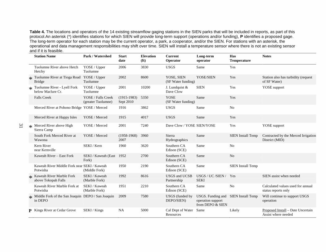
31

Table 4. The locations and operators of the 14 existing streamflow gaging stations in the SIEN parks that will be included in reports, as part of this protocol.An asterisk (*) identifies stations for which SIEN will provide long-term support (operations and/or funding), P identifies a proposed gage. The long-term operator for each station may be the current operator, a park, a cooperator, and/or the SIEN. For stations with an asterisk, the operational and data management responsibilities may shift over time. SIEN will install a temperature sensor where there is not an existing sensor and if it is feasible. Station Name Park / Watershed Start

date Elevation (ft)

Current Operator

Long-term operator

Has Temperature

Notes

Tuolumne River above Hetch Hetchy

YOSE / Upper Tuolumne

2006 3830 USGS

Same Yes

* Tuolumne River at Tioga Road Bridge


2002 8600 YOSE, SIEN (SF Water funding)

YOSE/SIEN Yes Station also has turbidity (request of SF Water)

* Tuolumne River - Lyell Fork below Maclure Cr.


2001 10200 J. Lundquist & Dave Clow

SIEN Yes YOSE support

Falls Creek YOSE / Falls Creek (greater Tuolumne)

(1915-1983) Sept 2010

5350 YOSE (SF Water funding)

Same Yes

Merced River at Pohono Bridge YOSE / Merced 1916 3862 USGS Same No

Merced River at Happy Isles YOSE / Merced 1915 4017 USGS Same Yes

* Merced River above High Sierra Camp

YOSE / Merced 2001 7240 Dave Clow / YOSE SIEN/YOSE Yes YOSE support

South Fork Merced River at Wawona

YOSE / Merced (1958-1968) 2007

3960 Sierra Hydrographics

Same SIEN Install Temp Contracted by the Merced Irrigation District (MID)

Kern River near Kernville

SEKI / Kern 1960 3620 Southern CA Edison (SCE)

Same No

Kaweah River – East Fork SEKI / Kaweah (East Fork)

1952 2700 Southern CA Edison (SCE)

Same No

Kaweah River Middle Fork near Potwisha

SEKI / Kaweah (Middle Fork)


Same SIEN Install Temp

* Kaweah River Marble Fork above Tokopah Falls

SEKI / Kaweah (Marble Fork)

1992 8616 USGS and UCSB Partnership

USGS / UC /SIEN / SEKI

Yes SIEN assist when needed

Kaweah River Marble Fork at Potwisha

SEKI / Kaweah (Marble Fork)


Same No Calculated values used for annual status reports only

* Middle Fork of the San Joaquin in DEPO

DEPO / San Joaquin 2009 7580 USGS (funded by DEPO/SIEN)

USGS. Funding and operation support from DEPO & SIEN

SIEN Install Temp Will continue to support USGS operation

P Kings River at Cedar Grove SEKI / Kings NA 5000 Cal Dept of Water Resources

Same Likely Proposed Install – Date Uncertain Assist where needed

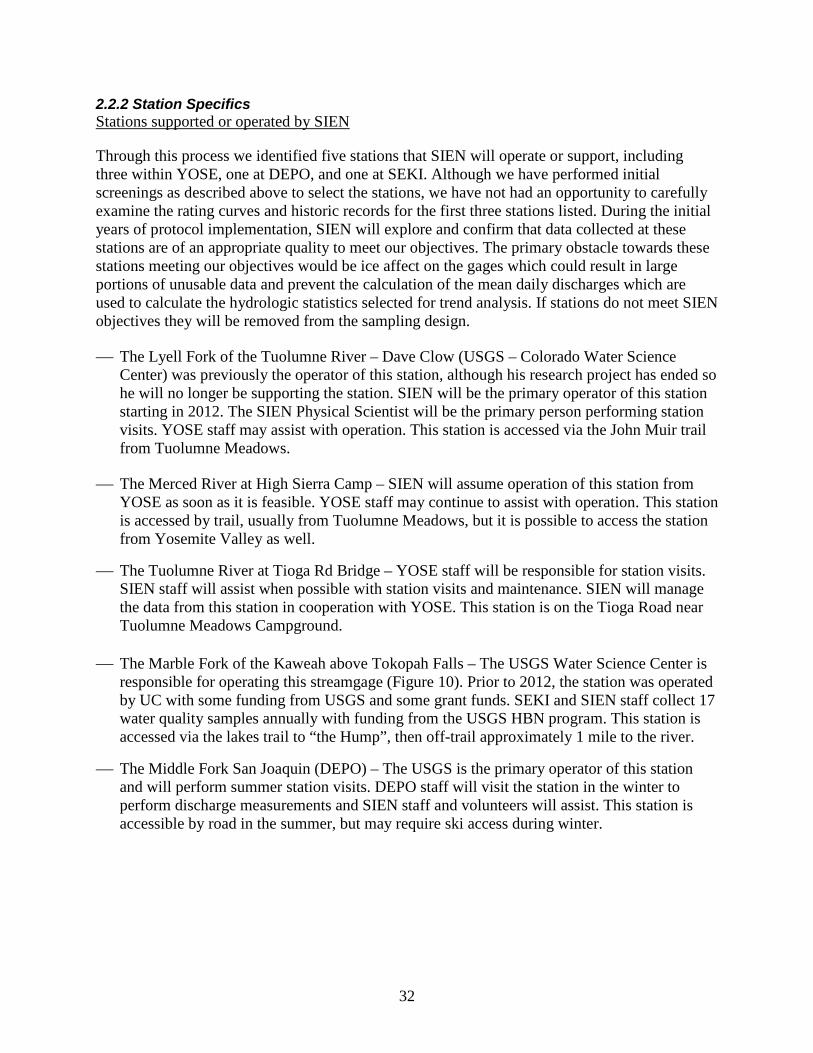
32

2.2.2 Station Specifics

Through this process we identified five stations that SIEN will operate or support, including three within YOSE, one at DEPO, and one at SEKI. Although we have performed initial screenings as described above to select the stations, we have not had an opportunity to carefully examine the rating curves and historic records for the first three stations listed. During the initial years of protocol implementation, SIEN will explore and confirm that data collected at these stations are of an appropriate quality to meet our objectives. The primary obstacle towards these stations meeting our objectives would be ice affect on the gages which could result in large portions of unusable data and prevent the calculation of the mean daily discharges which are used to calculate the hydrologic statistics selected for trend analysis. If stations do not meet SIEN objectives they will be removed from the sampling design.

Stations supported or operated by SIEN

The Lyell Fork of the Tuolumne River – Dave Clow (USGS – Colorado Water Science Center) was previously the operator of this station, although his research project has ended so he will no longer be supporting the station. SIEN will be the primary operator of this station starting in 2012. The SIEN Physical Scientist will be the primary person performing station visits. YOSE staff may assist with operation. This station is accessed via the John Muir trail from Tuolumne Meadows.

The Merced River at High Sierra Camp – SIEN will assume operation of this station from YOSE as soon as it is feasible. YOSE staff may continue to assist with operation. This station is accessed by trail, usually from Tuolumne Meadows, but it is possible to access the station from Yosemite Valley as well.

The Tuolumne River at Tioga Rd Bridge – YOSE staff will be responsible for station visits. SIEN staff will assist when possible with station visits and maintenance. SIEN will manage the data from this station in cooperation with YOSE. This station is on the Tioga Road near Tuolumne Meadows Campground.

The Marble Fork of the Kaweah above Tokopah Falls – The USGS Water Science Center is

responsible for operating this streamgage (Figure 10). Prior to 2012, the station was operated by UC with some funding from USGS and some grant funds. SEKI and SIEN staff collect 17 water quality samples annually with funding from the USGS HBN program. This station is accessed via the lakes trail to “the Hump”, then off-trail approximately 1 mile to the river.

The Middle Fork San Joaquin (DEPO) – The USGS is the primary operator of this station and will perform summer station visits. DEPO staff will visit the station in the winter to perform discharge measurements and SIEN staff and volunteers will assist. This station is accessible by road in the summer, but may require ski access during winter.

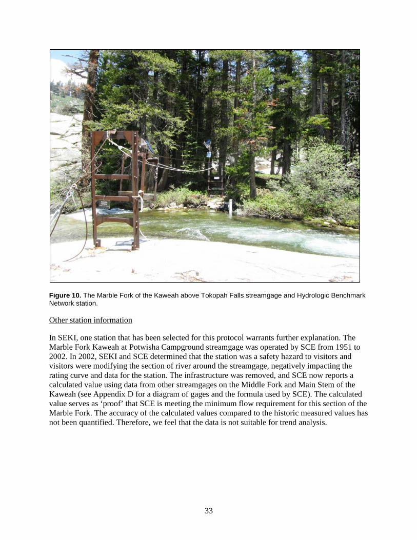
33

Figure 10. The Marble Fork of the Kaweah above Tokopah Falls streamgage and Hydrologic Benchmark Network station.

In SEKI, one station that has been selected for this protocol warrants further explanation. The Marble Fork Kaweah at Potwisha Campground streamgage was operated by SCE from 1951 to 2002. In 2002, SEKI and SCE determined that the station was a safety hazard to visitors and visitors were modifying the section of river around the streamgage, negatively impacting the rating curve and data for the station. The infrastructure was removed, and SCE now reports a calculated value using data from other streamgages on the Middle Fork and Main Stem of the Kaweah (see Appendix D for a diagram of gages and the formula used by SCE). The calculated value serves as ‘proof’ that SCE is meeting the minimum flow requirement for this section of the Marble Fork. The accuracy of the calculated values compared to the historic measured values has not been quantified. Therefore, we feel that the data is not suitable for trend analysis.

Other station information

34

2.3 Selected Measures Parameters selected for the rivers protocol reflect SIEN’s overall approach to monitor resource condition by using parameters that most strongly affect or reflect ecosystem function and are sensitive to multiple stressors, including future and unknown threats.

2.3.1 Hydrologic parameters Water level (stage) data is collected continuously, usually at 15-minute or hourly intervals, at all streamgages. These data are used to calculate continuous discharge across the period of record, and discharge data are used to calculate hydrologic parameters that reflect the quantity and timing of streamflow (Table 5). Rating curves are used to convert water level measurements into discharge. To develop the rating curve, instantaneous discharge and water level measurements are collected simultaneously across a range of streamflows to establish the relationship between water level and discharge. After establishing the rating curve, stage and discharge measurements are collected periodically to improve or update the rating curve. The mean daily and mean annual discharges are calculated from the continuous record of 15-minute water level data. All water quantity parameters are based on the hydrologic year (or water year (WY)) – October 1 through September 30. Some parameters, such as peak snowmelt runoff and center timing, are reported in number of days from the start of the water year and others, such as days to onset of snowmelt are reported as the number of days from the start of the calendar year.

Water level and discharge measurements will be recorded and reported in English units, which is the USGS standard. Guidance on measurement precision and reporting accuracy is included in the Quality Assurance Plan (SOP 10).

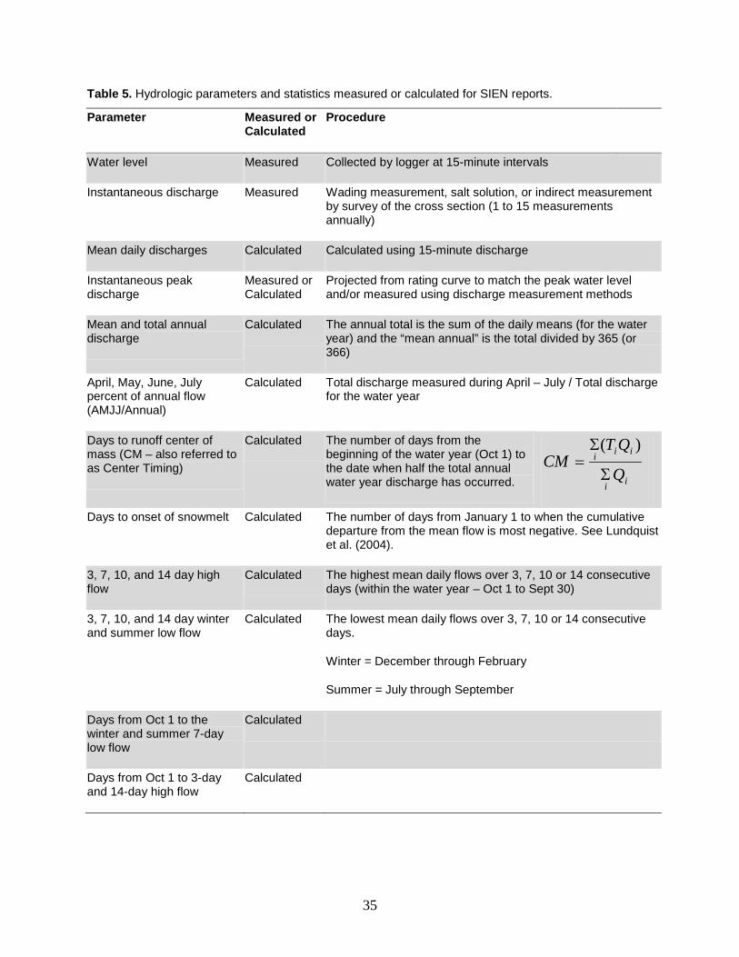
35

Table 5. Hydrologic parameters and statistics measured or calculated for SIEN reports.

Parameter Measured or Calculated

Procedure

Water level Measured Collected by logger at 15-minute intervals

Instantaneous discharge Measured Wading measurement, salt solution, or indirect measurement by survey of the cross section (1 to 15 measurements annually)

Mean daily discharges Calculated Calculated using 15-minute discharge

Instantaneous peak discharge

Measured or Calculated

Projected from rating curve to match the peak water level and/or measured using discharge measurement methods

Mean and total annual discharge

Calculated The annual total is the sum of the daily means (for the water year) and the “mean annual” is the total divided by 365 (or 366)

April, May, June, July percent of annual flow (AMJJ/Annual)

Calculated Total discharge measured during April – July / Total discharge for the water year

Days to runoff center of mass (CM – also referred to as Center Timing)

Calculated The number of days from the beginning of the water year (Oct 1) to the date when half the total annual water year discharge has occurred. ii

iii

Q

QTCM

Σ

Σ=

)(

Days to onset of snowmelt Calculated The number of days from January 1 to when the cumulative departure from the mean flow is most negative. See Lundquist et al. (2004).

3, 7, 10, and 14 day high flow

Calculated The highest mean daily flows over 3, 7, 10 or 14 consecutive days (within the water year – Oct 1 to Sept 30)

3, 7, 10, and 14 day winter and summer low flow

Calculated The lowest mean daily flows over 3, 7, 10 or 14 consecutive days.

Winter = December through February

Summer = July through September

Days from Oct 1 to the winter and summer 7-day low flow

Calculated

Days from Oct 1 to 3-day and 14-day high flow

Calculated

36

2.3.2 Water chemistry parameters In addition to water quantity information (i.e., discharge and stage), the NPS Water Resources Division (WRD) recommended that a set of core water quality parameters (water temperature, dissolved oxygen, pH, specific conductance) be measured in all NPS I&M Network park units as part of the aquatic vital signs monitoring efforts (NPS 2002). We will monitor water temperature at selected streamgages and a greater set of water chemistry parameters, including the four core parameters, at the two Hydrologic Benchmark Network (HBN) stations (Table 6). Water temperature was selected for monitoring at a greater number of stations because it can be monitored continuously in conjunction with the water stage data and the sensor calibration does not need to occur as frequently as other water chemistry parameters. Other core water quality parameters, such as pH and dissolved oxygen, are not being monitored at these stations because these sensors require frequent calibration, the project budget cannot accommodate the time and staff to make frequent visits to these stations, and because the dilute nature of SIEN surface waters makes in situ measurement of these parameters difficult.

Table 6. Water chemistry parameters collected or analyzed for SIEN reports.

Parameter Procedure Frequency Data Storage

Mos

t sta

tions

(w

here

pos

sibl

e) Water Temperature Automated sensor

at streamgage station

Hourly - Continuous

Stored on SIEN server and in SIEN Rivers SQL Server Database

HBN

sta

tions

in Y

OS

E &

SEKI

- pH, dissolved oxygen, specific conductance, alkalinity

Grab sample analyzed at USGS laboratory in Colorado

Collected by YOSE and SEKI staff with assistance from SIEN during 14 visits per year at one station in SEKI and one station in YOSE

Stored in the USGS NWIS database.

Not stored by SIEN.

-Major ions: Ca, Na, Mg, K, Cl, SO4

-Dissolved organic carbon (DOC), nitrate and nitrite (NO3+NO2), total nitrogen (TN), particulate carbon, total phosphorous

Through the USGS HBN program, water samples are collected during 17 visits per year at one station in SEKI and one station in YOSE to characterize an array of water chemistry parameters, including pH, dissolved oxygen, specific conductance, alkalinity, major ions, dissolved organic carbon (DOC), particulate carbon (PC), nitrate and nitrite (NO3+NO2), total phosphorous, and total nitrogen (TN). These samples will be collected by YOSE, SEKI, and SIEN staff with financial support from USGS. The samples are analyzed at the USGS lab in Colorado. The resulting data will be stored on the USGS NWIS server and managed by the USGS. We will obtain the data from the USGS NWIS site for reporting purposes. 2.4 Power and Trend Analysis Starcevich and Kane completed a trend and power analysis using historic data from two long-term streamgages in the SIEN (see Appendix C). The report examines long-term trends for 18

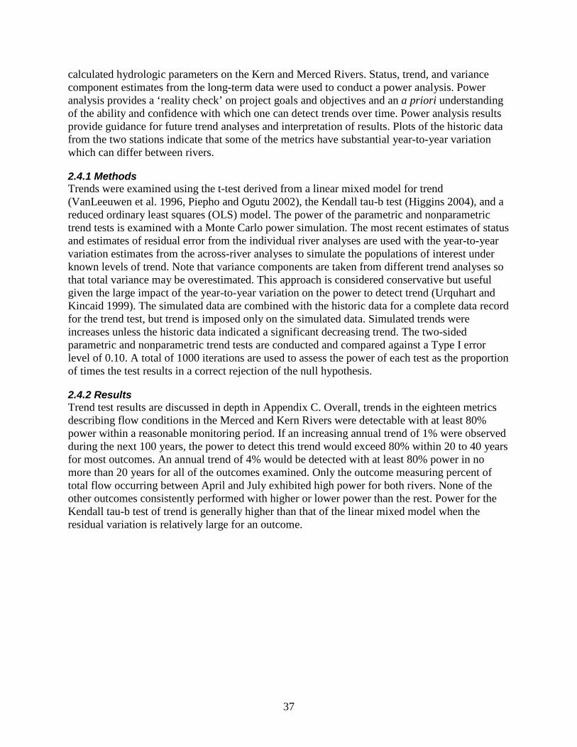
37

calculated hydrologic parameters on the Kern and Merced Rivers. Status, trend, and variance component estimates from the long-term data were used to conduct a power analysis. Power analysis provides a ‘reality check’ on project goals and objectives and an a priori understanding of the ability and confidence with which one can detect trends over time. Power analysis results provide guidance for future trend analyses and interpretation of results. Plots of the historic data from the two stations indicate that some of the metrics have substantial year-to-year variation which can differ between rivers.

2.4.1 Methods Trends were examined using the t-test derived from a linear mixed model for trend (VanLeeuwen et al. 1996, Piepho and Ogutu 2002), the Kendall tau-b test (Higgins 2004), and a reduced ordinary least squares (OLS) model. The power of the parametric and nonparametric trend tests is examined with a Monte Carlo power simulation. The most recent estimates of status and estimates of residual error from the individual river analyses are used with the year-to-year variation estimates from the across-river analyses to simulate the populations of interest under known levels of trend. Note that variance components are taken from different trend analyses so that total variance may be overestimated. This approach is considered conservative but useful given the large impact of the year-to-year variation on the power to detect trend (Urquhart and Kincaid 1999). The simulated data are combined with the historic data for a complete data record for the trend test, but trend is imposed only on the simulated data. Simulated trends were increases unless the historic data indicated a significant decreasing trend. The two-sided parametric and nonparametric trend tests are conducted and compared against a Type I error level of 0.10. A total of 1000 iterations are used to assess the power of each test as the proportion of times the test results in a correct rejection of the null hypothesis.

2.4.2 Results Trend test results are discussed in depth in Appendix C. Overall, trends in the eighteen metrics describing flow conditions in the Merced and Kern Rivers were detectable with at least 80% power within a reasonable monitoring period. If an increasing annual trend of 1% were observed during the next 100 years, the power to detect this trend would exceed 80% within 20 to 40 years for most outcomes. An annual trend of 4% would be detected with at least 80% power in no more than 20 years for all of the outcomes examined. Only the outcome measuring percent of total flow occurring between April and July exhibited high power for both rivers. None of the other outcomes consistently performed with higher or lower power than the rest. Power for the Kendall tau-b test of trend is generally higher than that of the linear mixed model when the residual variation is relatively large for an outcome.

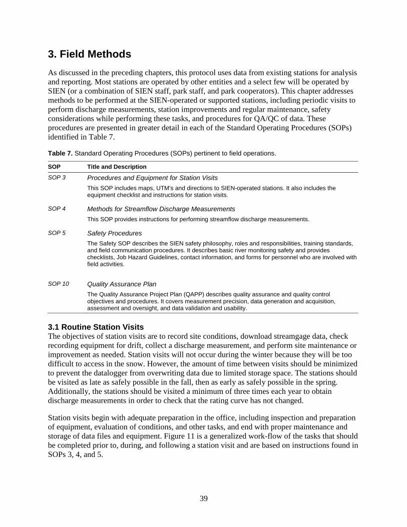
39

3. Field Methods As discussed in the preceding chapters, this protocol uses data from existing stations for analysis and reporting. Most stations are operated by other entities and a select few will be operated by SIEN (or a combination of SIEN staff, park staff, and park cooperators). This chapter addresses methods to be performed at the SIEN-operated or supported stations, including periodic visits to perform discharge measurements, station improvements and regular maintenance, safety considerations while performing these tasks, and procedures for QA/QC of data. These procedures are presented in greater detail in each of the Standard Operating Procedures (SOPs) identified in Table 7.

Table 7. Standard Operating Procedures (SOPs) pertinent to field operations.

SOP Title and Description

SOP 3 Procedures and Equipment for Station Visits This SOP includes maps, UTM’s and directions to SIEN-operated stations. It also includes the

equipment checklist and instructions for station visits.

SOP 4 Methods for Streamflow Discharge Measurements This SOP provides instructions for performing streamflow discharge measurements.

SOP 5 Safety Procedures The Safety SOP describes the SIEN safety philosophy, roles and responsibilities, training standards,

and field communication procedures. It describes basic river monitoring safety and provides checklists, Job Hazard Guidelines, contact information, and forms for personnel who are involved with field activities.

SOP 10 Quality Assurance Plan The Quality Assurance Project Plan (QAPP) describes quality assurance and quality control

objectives and procedures. It covers measurement precision, data generation and acquisition, assessment and oversight, and data validation and usability.

3.1 Routine Station Visits The objectives of station visits are to record site conditions, download streamgage data, check recording equipment for drift, collect a discharge measurement, and perform site maintenance or improvement as needed. Station visits will not occur during the winter because they will be too difficult to access in the snow. However, the amount of time between visits should be minimized to prevent the datalogger from overwriting data due to limited storage space. The stations should be visited as late as safely possible in the fall, then as early as safely possible in the spring. Additionally, the stations should be visited a minimum of three times each year to obtain discharge measurements in order to check that the rating curve has not changed.

Station visits begin with adequate preparation in the office, including inspection and preparation of equipment, evaluation of conditions, and other tasks, and end with proper maintenance and storage of data files and equipment. Figure 11 is a generalized work-flow of the tasks that should be completed prior to, during, and following a station visit and are based on instructions found in SOPs 3, 4, and 5.

40

Figure 11. A generalized workflow for office preparation and procedures for streamgage station visits. See SOPs 3, 4, and 5 for more details.

Office preparation includes assembly of field equipment and safety gear (SOP 3), review of safety procedures (SOP 5), and an estimation of flows at the site(s) to be visited. SIEN will store most equipment in the Tuolumne Meadows water lab at YOSE. An estimation of flow is needed to determine the safest and most suitable method for discharge measurement (i.e., wading during lower flows or dye tracer during high flows). Although not all SIEN gages have real-time data available via satellite, it is possible to view some stations online to get a general sense of whether flows are rising, falling, or remaining steady. We can use data from these online gages to assess conditions at those that are not online because major rivers and tributaries exhibit similar streamflow timing throughout the SIEN. For example, if the stage has been rising for multiple days at the Tuolumne River at Tioga Rd Bridge, it can be assumed that streamflow at the Lyell Fork station, which is further up in the watershed, would be too high for wading.

During station visits, the following actions will be performed: 1. Photo documentation of site conditions 2. Water level and discharge measurement 3. Water quality measurement for quality control checks of the continuous temperature

sensor 4. Streamgage datalogger download. 5. Maintenance or repair actions as needed

41

All streamgages that SIEN plans to operate record both water level and water temperature. Station visit procedures include a water quality measurement near the continuous water temperature sensor. The purpose of the instantaneous measurement is to check for drift in the sensor. The handheld water quality meter also measures dissolved oxygen and conductivity, which we will record on our field datasheet. We will not use the data from the instantaneous measurements for analysis or reporting, but will use the temperature measurement to perform data correction on the continuous temperature data. Additional data to be recorded on the datasheet includes information about the streamgage data download and streamflow discharge measurement data (see SOP 3).

3.1.1 Discharge Measurements During routine station visits, discharge measurements are performed and qualitative descriptions of the discharge measurement site such as cross-section and control conditions are recorded on the datasheet prior to the measurement. During any visit, selection of the appropriate method will depend on the site, intensity of flow, and access conditions (see SOPs 3 and 4 for guidance on method selection). Each of these methods requires specific specialized equipment and procedures. For the most part, discharge will be measured quantitatively using established USGS procedures (Turnipseed and Sauer 2010). Quantitative methods that will be used by SIEN include: 1) wading, 2) dye tracer method, 3) survey method, and 4) measurement from a bridge. The most commonly used method will be wading using vertical axis current meters (pygmy and Price AA). Dye tracer and bridge measurements are used when conditions prevent safe wading. Semi-quantitative discharge estimates may also be made using floats under extreme high flow conditions. Surveys are used following a high flow event to estimate the discharge based on channel characteristics. Bridge measurements can only be performed at one SIEN station, the Tuolumne River at Tioga Rd Bridge. No estimate of subsurface flows will be done under this monitoring protocol.

Bridge based or wading current meter discharge estimates follow the same basic procedures. A cross-section of the stream is chosen and the stream is divided into panels or sections. The width, depth, and velocity of each section are then recorded and individual discharge measurements per section are computed. Total stream discharge is the sum of individual discharge measurements in each section and is recorded in cubic feet per second (ft3/s or cfs). The current meter measures velocity at a single point. Discharge measurements are based on the mean vertical velocity obtained from each measured section, which is derived from depth-integrated measurements within the vertical profile (Figure 12).

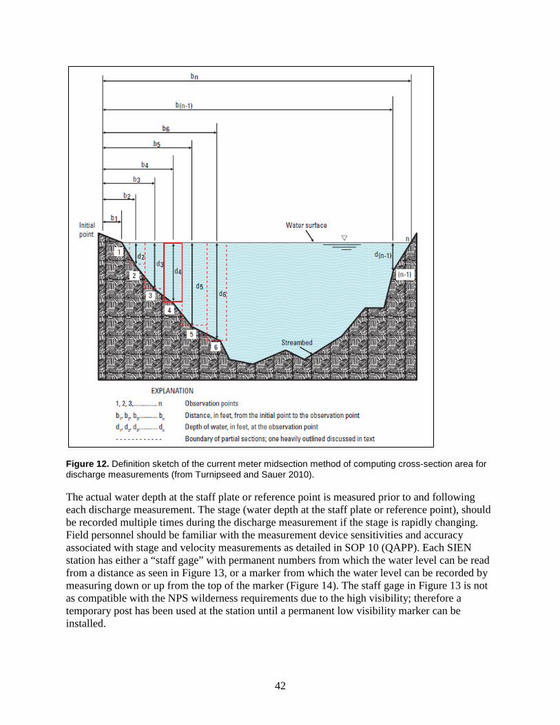
42

Figure 12. Definition sketch of the current meter midsection method of computing cross-section area for discharge measurements (from Turnipseed and Sauer 2010).

The actual water depth at the staff plate or reference point is measured prior to and following each discharge measurement. The stage (water depth at the staff plate or reference point), should be recorded multiple times during the discharge measurement if the stage is rapidly changing. Field personnel should be familiar with the measurement device sensitivities and accuracy associated with stage and velocity measurements as detailed in SOP 10 (QAPP). Each SIEN station has either a “staff gage” with permanent numbers from which the water level can be read from a distance as seen in Figure 13, or a marker from which the water level can be recorded by measuring down or up from the top of the marker (Figure 14). The staff gage in Figure 13 is not as compatible with the NPS wilderness requirements due to the high visibility; therefore a temporary post has been used at the station until a permanent low visibility marker can be installed.

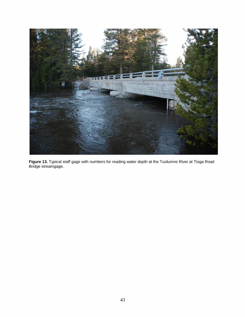
43

Figure 13. Typical staff gage with numbers for reading water depth at the Tuolumne River at Tioga Road Bridge streamgage.

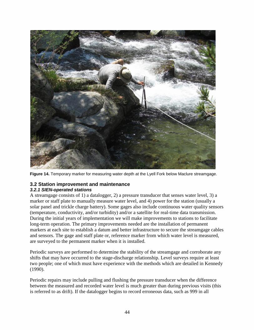
44

Figure 14. Temporary marker for measuring water depth at the Lyell Fork below Maclure streamgage.

3.2 Station improvement and maintenance 3.2.1 SIEN-operated stations A streamgage consists of 1) a datalogger, 2) a pressure transducer that senses water level, 3) a marker or staff plate to manually measure water level, and 4) power for the station (usually a solar panel and trickle charge battery). Some gages also include continuous water quality sensors (temperature, conductivity, and/or turbidity) and/or a satellite for real-time data transmission. During the initial years of implementation we will make improvements to stations to facilitate long-term operation. The primary improvements needed are the installation of permanent markers at each site to establish a datum and better infrastructure to secure the streamgage cables and sensors. The gage and staff plate or, reference marker from which water level is measured, are surveyed to the permanent marker when it is installed.

Periodic surveys are performed to determine the stability of the streamgage and corroborate any shifts that may have occurred to the stage-discharge relationship. Level surveys require at least two people; one of which must have experience with the methods which are detailed in Kennedy (1990).

Periodic repairs may include pulling and flushing the pressure transducer when the difference between the measured and recorded water level is much greater than during previous visits (this is referred to as drift). If the datalogger begins to record erroneous data, such as 999 in all

45

columns, we will first check the sensors, then troubleshoot the operating program with the Campbell Scientific technical support, and then replace equipment as needed.

Over time, SIEN will need to repair or replace equipment. Many of our stations will experience freezing conditions; thus, we must utilize equipment that will work best in such conditions. Further, we must choose equipment that is of good quality, but not so expensive that we cannot afford to replace it periodically. There are many equipment options for stream gaging at a wide range of prices. SIEN will attempt to utilize the same type of streamgage equipment at all the stations we operate. Campbell Scientific data loggers are widely used for streamgages and are the primary type used at the SIEN stations. Campbell Scientific carries nearly all the equipment needed for a complete streamgage including pressure transducers and water chemistry sensors.

SIEN will follow permitting requirements prior to completing improvement actions at the streamgages that we operate. Initially, SIEN will only be operating stations in YOSE. The YOSE requirements involve: 1) submitting a research permit, 2) submitting a Minimum Requirements Analysis (MRAs) and working with the park to modify our actions and the MRA until it is approved, and 3) inputting all information to Planning, Environment and Public Comment (PEPC) database. Additionally, we will renew the research permit annually. The permitting processes are required to ensure that our activities comply with park regulations and wilderness character.

Permitting and compliance

3.2.2 Other stations We will install Hobo temperature loggers at three stations that are within the SIEN parks. These are stations that the SIEN does not operate, but where the operator has agreed to allow a temperature logger to be added. SOP 3 includes instructions for installing and downloading the temperature loggers.

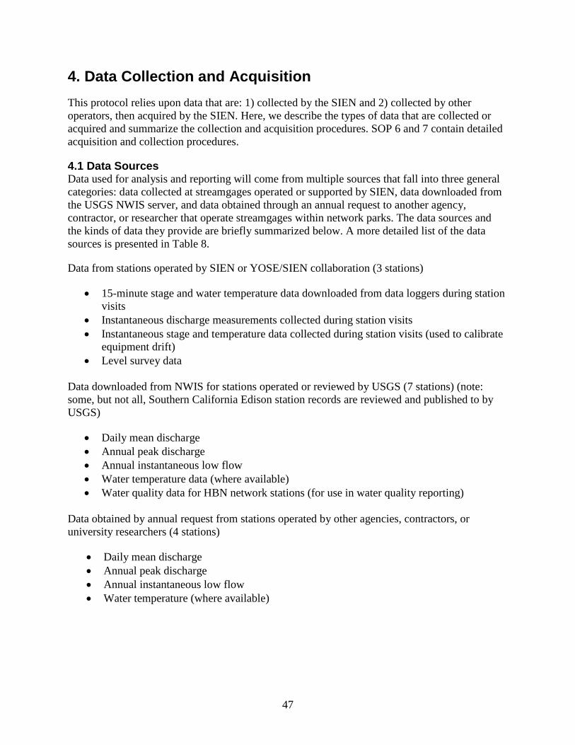
47

4. Data Collection and Acquisition This protocol relies upon data that are: 1) collected by the SIEN and 2) collected by other operators, then acquired by the SIEN. Here, we describe the types of data that are collected or acquired and summarize the collection and acquisition procedures. SOP 6 and 7 contain detailed acquisition and collection procedures.

4.1 Data Sources Data used for analysis and reporting will come from multiple sources that fall into three general categories: data collected at streamgages operated or supported by SIEN, data downloaded from the USGS NWIS server, and data obtained through an annual request to another agency, contractor, or researcher that operate streamgages within network parks. The data sources and the kinds of data they provide are briefly summarized below. A more detailed list of the data sources is presented in Table 8.

Data from stations operated by SIEN or YOSE/SIEN collaboration (3 stations)

• 15-minute stage and water temperature data downloaded from data loggers during station visits

• Instantaneous discharge measurements collected during station visits • Instantaneous stage and temperature data collected during station visits (used to calibrate

equipment drift) • Level survey data

Data downloaded from NWIS for stations operated or reviewed by USGS (7 stations) (note: some, but not all, Southern California Edison station records are reviewed and published to by USGS)

• Daily mean discharge • Annual peak discharge • Annual instantaneous low flow • Water temperature data (where available) • Water quality data for HBN network stations (for use in water quality reporting)

Data obtained by annual request from stations operated by other agencies, contractors, or university researchers (4 stations)

• Daily mean discharge • Annual peak discharge • Annual instantaneous low flow • Water temperature (where available)

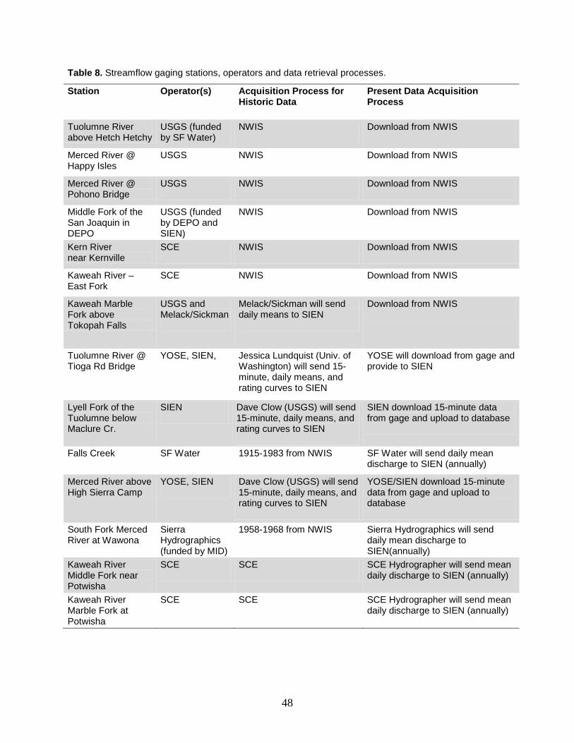
48

Table 8. Streamflow gaging stations, operators and data retrieval processes.

Station Operator(s) Acquisition Process for Historic Data

Present Data Acquisition Process


USGS (funded by SF Water)

NWIS Download from NWIS

Merced River @ Happy Isles

USGS NWIS Download from NWIS

Merced River @ Pohono Bridge

USGS NWIS Download from NWIS

Middle Fork of the San Joaquin in DEPO

USGS (funded by DEPO and SIEN)

NWIS Download from NWIS

Kern River near Kernville

SCE NWIS Download from NWIS

Kaweah River – East Fork

SCE NWIS Download from NWIS

Kaweah Marble Fork above Tokopah Falls

USGS and Melack/Sickman

Melack/Sickman will send daily means to SIEN

Download from NWIS

Tuolumne River @ Tioga Rd Bridge

YOSE, SIEN, Jessica Lundquist (Univ. of Washington) will send 15-minute, daily means, and rating curves to SIEN

YOSE will download from gage and provide to SIEN

Lyell Fork of the Tuolumne below Maclure Cr.

SIEN Dave Clow (USGS) will send 15-minute, daily means, and rating curves to SIEN

SIEN download 15-minute data from gage and upload to database

Falls Creek SF Water 1915-1983 from NWIS SF Water will send daily mean discharge to SIEN (annually)

Merced River above High Sierra Camp

YOSE, SIEN Dave Clow (USGS) will send 15-minute, daily means, and rating curves to SIEN

YOSE/SIEN download 15-minute data from gage and upload to database

South Fork Merced River at Wawona

Sierra Hydrographics (funded by MID)

1958-1968 from NWIS Sierra Hydrographics will send daily mean discharge to SIEN(annually)

Kaweah River Middle Fork near Potwisha

SCE SCE SCE Hydrographer will send mean daily discharge to SIEN (annually)

Kaweah River Marble Fork at Potwisha

SCE SCE SCE Hydrographer will send mean daily discharge to SIEN (annually)

49

4.2 Data Collection and Acquisition A general overview of the data types, acquisition, collection, and processing is illustrated in Figure 15. Much of this program’s data management occurs within the multi-faceted Aquarius software platform which is explained in the following chapter and SOP 7. Data from streamgages operated by SIEN will include river stage and water temperature recorded at 15-minute intervals by automated dataloggers and instantaneous discharge measurements collected during periodic station visits. Continuous data are downloaded from the datalogger to a mini-laptop computer in the field. Instantaneous discharge measurements are collected with a current meter and AquaCalc, a handheld device that records the depth and velocity in each cross-section, then calculates and stores the total discharge. Current meters are routinely calibrated as outlined in the project quality assurance plan (SOP 10). Upon return to the office, the files from the laptop and AquaCalc are transferred to the SIEN file server and stored as read-only versions. The data are uploaded, edited, and stored to the SQL server database using the Aquarius software (see SOP 7).

The records from all stations that the USGS operates or reviews are available through the National Water Information System (NWIS). The mean annual discharge and instantaneous peak and low flow data can be obtained from NWIS using the Import from Data Portal toolbox within the Aquarius software. Alternately, if the Aquarius Data Portal toolbox does not allow access to the most recent data, the data can be downloaded in tab delimited format from NWIS and uploaded to Aquarius with the Import from File toolbox as described in SOP 6.

Data from stations operated by other agencies, contractors, and universities that are not available through NWIS are obtained by request from the operator. Initially, all historic data are acquired and imported, and saved to the database. In subsequent years, only data from the most recent water year is requested. These data are acquired as excel files that are saved as comma separated values (.csv) files, then imported using Aquarius Springboard. Aquarius provides the ability to define the structure of the imported data and easily restructure it so it can be saved to the Aquarius SQL server database using the Write to Server toolbox. Data from several of the stations are posted to the California Dept of Water Resources online data repository, the California Data Exchange Center (CDEC). The CDEC site posts data in real time to provide information to water users throughout the state. Because the data are real-time, the data are qualified as preliminary and should not be acquired by the SIEN. Rather, SIEN will acquire the data from the operator of each station. SOP 6 includes instructions for requesting data, naming and saving the files locally, while SOP 7 includes instructions for importing and saving the files within Aquarius.

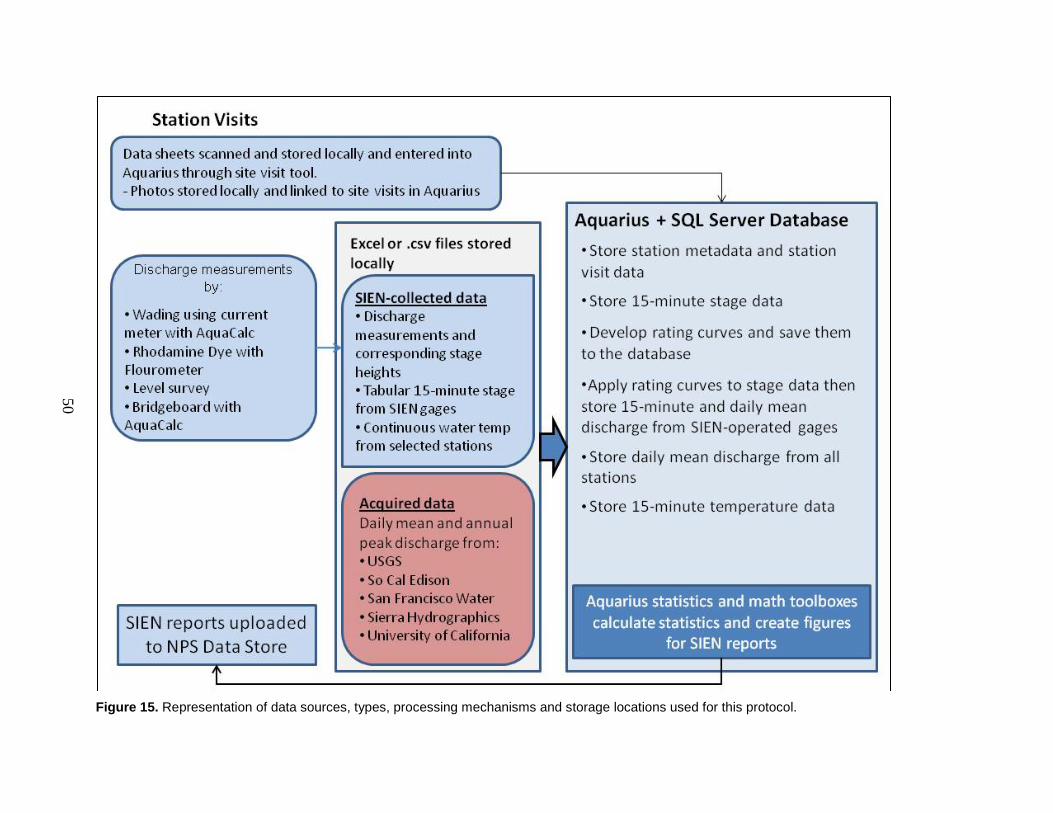
50

Figure 15. Representation of data sources, types, processing mechanisms and storage locations used for this protocol.

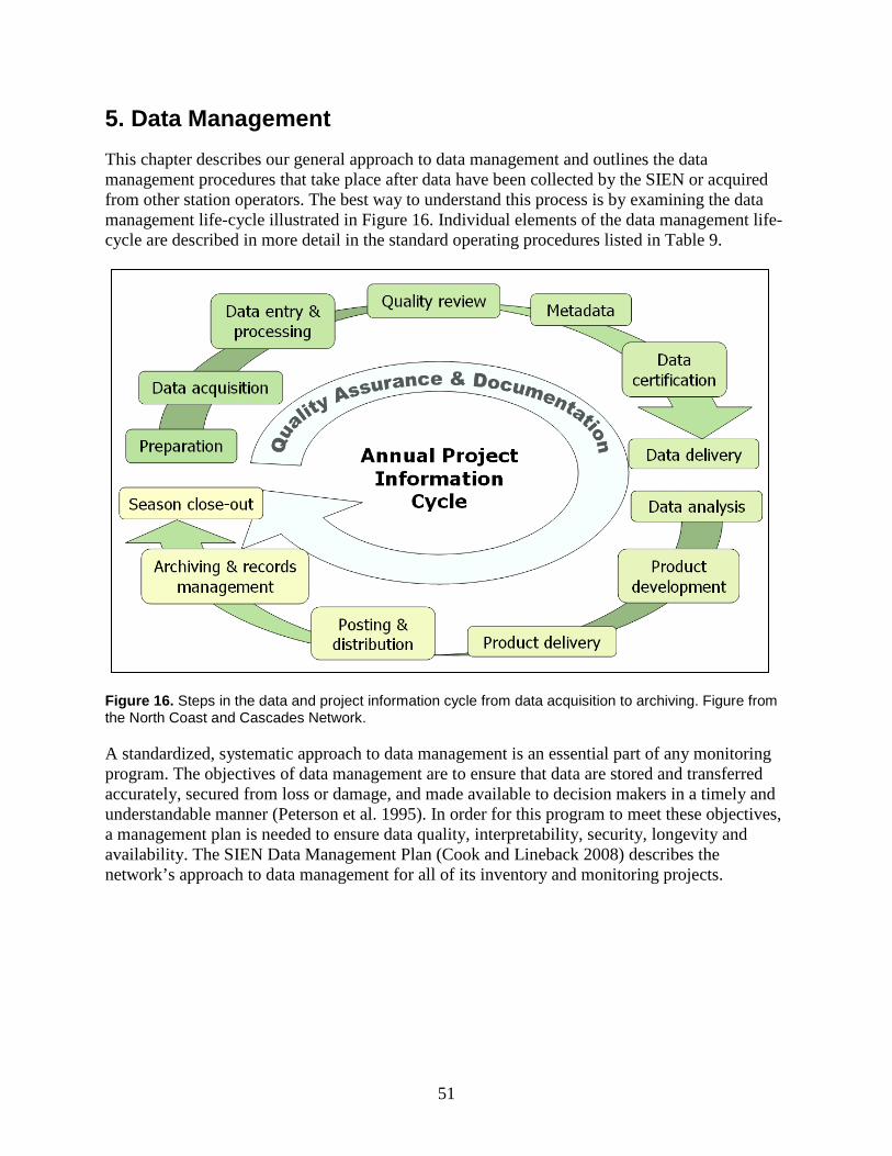
51

5. Data Management This chapter describes our general approach to data management and outlines the data management procedures that take place after data have been collected by the SIEN or acquired from other station operators. The best way to understand this process is by examining the data management life-cycle illustrated in Figure 16. Individual elements of the data management life-cycle are described in more detail in the standard operating procedures listed in Table 9.

Figure 16. Steps in the data and project information cycle from data acquisition to archiving. Figure from the North Coast and Cascades Network.

A standardized, systematic approach to data management is an essential part of any monitoring program. The objectives of data management are to ensure that data are stored and transferred accurately, secured from loss or damage, and made available to decision makers in a timely and understandable manner (Peterson et al. 1995). In order for this program to meet these objectives, a management plan is needed to ensure data quality, interpretability, security, longevity and availability. The SIEN Data Management Plan (Cook and Lineback 2008) describes the network’s approach to data management for all of its inventory and monitoring projects.

52

Table 9. Standard Operating Procedures pertinent to data management activities.

SOP Title and Description SOP 6 Acquiring Water Quality and Streamflow Data from Streamgage Operators

This SOP contains procedures for acquiring summarized streamgage data for those stations that are not operated by the SIEN. Instructions are included for naming and storing these data files locally.

SOP 7 Data Management This is SOP includes an introduction to the Aquarius software and database. It explains how

Aquarius will be utilized for many of the data management and analysis procedures associated with this protocol. It includes instructions for importing all data to the database, joining and correcting the data, establishing and managing rating curves, applying rating curves to water level data, summarizing data in preparation for data analysis, and writing data to the SQL server database.

SOP 10 Quality Assurance Project Plan The Quality Assurance Project Plan (QAPP) describes quality assurance and quality control

objectives and procedures. It covers an overview of data management, documentation, records management, review, verification, validation, and reconciliation.

Data take on different forms during various phases of a project, and are maintained in different places as they are acquired, processed, documented, analyzed, reported, and distributed. Here, we outline the data management activities and the software used to store and process data for analyses and summary reports. Effective data management requires a comprehensive project information management strategy that is detailed and structured within an annual cycle, designed for refinement as needed, and is sustainable throughout the lifecycle of the protocol. Primary responsibility for this project’s information management resides with the SIEN Physical Scientist and Data Manager but is not effectively implemented without the assistance of other network staff and cooperators.

5.1 Aquarius Software and SQL Server Database The database used by the SIEN Rivers Monitoring protocol resides on a Microsoft SQL Server managed by the NPS Water Resources Division (NPS WRD) at the Natural Resources Stewardship and Science (NRSS) Program Center in Fort Collins, CO. The WRD SQL server is accessed via a remote desktop connection to WRD’s 5-user license for Aquarius Software (Aquatic Informatics, Vancouver, BC). The Aquarius software provides two user interfaces (Aquarius Workstation and Springboard) and a logical framework (Aquarius Server) based on a proprietary database schema that integrates with Microsoft SQL Server to define table structures and relationships (See Appendix F for the data dictionary). Aquarius software is specifically designed to handle data that are continuiously collected at fixed stations, . Data from individual stations are stored in a single table as sequential events.Consequently the NPS WRD database does not conform to the NPS Natural Resources Database Template standards because complex table relationships are not required. However, it does meet the required standards for the NPStoret and EPA Storet data. The NPS-WRD SQL Server is managed by the primary NPS WRD Data Manager, Dean Tucker ([email protected]). He and NRSS IT staff are responsible for archiving and backup procedures.

mailto:[email protected]�

53

Aquarius is multi-faceted software that includes components to develop rating curves, correct data and record changes through versioning, visualize data, perform analysis and reporting tasks, and save the data to a SQL Server database (Aquatic Informatics 2011). Tutorials, software support, and a help desk are available to registered software users on the Aquarius website (http://www.aquaticinformatics.com/support-login).

The Aquarius Workstation includes the Whiteboard and Springboard. The Whiteboard provides data production toolboxes with modules that automate data importing, data QA/QC and rating curve development, while the Aquarius Springboard provides one click access to the most common tasks in environmental data management and production, such as uploading field visit data, importing logger files, managing monitoring locations, configuring derived datasets, and running reports. These data production modules are wired together by the user to create a custom workflow for importing, processing, analyzing, and exporting data. Aquarius “Server” is middleware that links the SQL Server database to the Workstation.

Aquarius’s central concept is the monitoring location, to which time series, rating curves, field visit information, and other data are attributed. Each monitoring location has associated metadata such as geospatial data, information about benchmarks at the gage, and equipment. All time series data must be associated with an established monitoring location. Figure 17 shows the Aquarius Springboard, the starting point for creating monitoring locations, editing metadata, and uploading or accessing data for other data management tasks. In addition, staff at Southwest Alaska Inventory and Monitoring Network (SWAN) have developed an MS Access form and SQL procedures that allow Aquarius to accommodate additional metadata required by NPStoret

The Aquarius software is the commercially available version of the software that USGS uses for their data management (called GRSAT). SWAN has been working with WRD to create a system of permissions and roles at the Aquarius and SQL Server level that will enable any of the 32 I&M networks to have their own network-based repository of continuous water quality and quantity data. The SIEN will create and update our data in the database which can also be accessed at the national level. This will allow for comparison of similar water quality/quantity parameters among all the NPS units, with associated metadata stored in the same system.

http://www.aquaticinformatics.com/support-login�

http://aquaticinformatics.com/product-feature/data-import�



http://aquaticinformatics.com/product-feature/location-management�

http://aquaticinformatics.com/aquarius-server�

http://aquaticinformatics.com/product-feature/rating-curves�

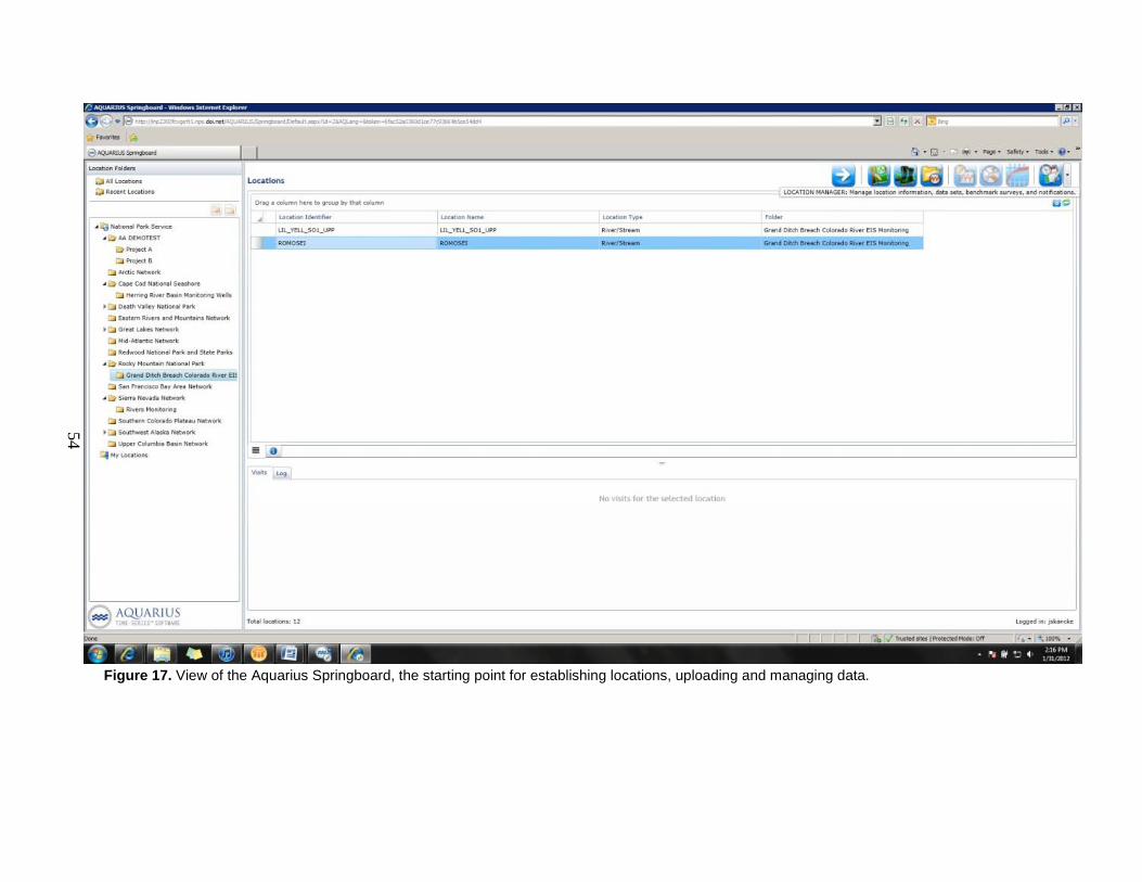
54

Figure 17. View of the Aquarius Springboard, the starting point for establishing locations, uploading and managing data.

55

5.2 Data Processing and Storage As outlined in previous chapters, data are collected or acquired by SIEN from a number of sources and in a variety of formats. After data have been acquired or collected, they are processed through mechanisms that are unique to the data type, then stored in the database and analyzed for reporting purposes. An overview of data processing procedures by data type is included here.

5.2.1 Discharge and water level data from SIEN-operated gages Instantaneous discharge and water level measurements that are collected and continuous water level data that are downloaded during station visits are stored on the network drive as read-only files immediately upon returning to the office. Instructions for the file naming, file formats, and network file folder location are described in SOP 3. The instantaneous discharge and water level measurements are uploaded to Aquarius and used for rating curve development. The data are input via the Aquarius Site Visit Tool along with the time and date of the measurements and links to site photos. The 15-minute water level data are imported to Aquarius in their original format using the Import from File toolbox, then examined for missing or erroneous data. In addition to drift that naturally occurs with water level and temperature loggers, it is likely that the water level sensors at SIEN-operated stations will be affected by ice. The water level data is adjusted using the Data Correction toolbox. After the rating curve has been developed or updated, it is applied to the corrected 15-minute water level data using the Aquarius Rating Curve Player toolbox. Next, the Descriptive Statistics toolbox is used to calculate the min, max, mean daily and mean annual discharge. All data, including the rating curves, are stored in the Aquarius SQL Server database using the Write to Server toolbox. Mean daily discharge values are used during data analysis to compute other hydrologic parameters. The methods for uploading and processing these data are provided in SOP 7.

5.2.2 Mean daily discharge acquired from streamgages operated or reviewed by USGS As described in the previous chapter, data from streamgages that are operated or reviewed by the USGS are posted to the USGS National Water Information System (NWIS) website. Mean daily discharge data are downloaded directly from NWIS to Aquarius or downloaded from NWIS, stored as comma separated values files on the SIEN server and imported to Aquarius (see SOP 6 for detailed instructions). The data are linked to the appropriate station in Aquarius and stored in the database. No further processing of the data will be required until they are analyzed along with the SIEN-collected data.

5.2.3 Mean daily discharge acquired from streamgage operators Mean daily discharge data are acquired and stored as read-only Excel spreadsheets following procedures described in SOP 6. The data are then saved as .csv files and uploaded to Aquarius using the Append Logger File Tool within Aquarius Springboard. When files are appended via the Aquarius Springboard, they are automatically saved in the database. The data do not require any further processing until they are analyzed along with the SIEN-collected data.

5.2.4 Continuous water temperature data Temperature data are uploaded to Aquarius in a similar manner as the 15-minute water level data (see SOP 7). Upon upload, the data are linked to a station and any instantaneous measurements are input using the Station Visit toolbox. Instantaneous measurements are used to assess instrument drift and then the Signal Joining and Signal Trimming toolboxes are used to perform

56

QA/QC, such as applying drift correction or removing outlying values. The raw and corrected data are then stored to the database.

5.3 Metadata Procedures The data manager at NPS WRD is working with Aquatic Informatics to allow for inclusion of all metadata fields required by the NPS, however the database does not currently allow for entry of all fields. Therefore, SIEN will create and store metadata compliant with the Federal Geographic Data Committee (FGDC) Metadata Standard and the National Biological Information Infrastructure (NBII) Biological Data Profile. Meeting these standards is prerequisite for uploading data to the NPS Data Store. We will develop an ArcGIS geodatabase that documents the locations of all the streamgages identified in this protocol. We will use the geodatabase to store FGDC compliant spatial metadata for each station. The geodatabase is routinely backed up by the SIEN data manager along with all SIEN data.

5.4 Data Standards To ensure scientific credibility, where we have the ability to do so, we intend to meet the following standards for streamflow and water chemistry data: (1) qualitative accuracy, (2) completeness, (3) consistency, (4) precision, (5) timeliness, (6) uniqueness, and (7) validity. Because this protocol relies on data harvested from sources other than our own direct collection, we will use established data providers whose data also meet these standards. Data qualifiers are normally reported with results to inform readers of important restrictions or limitations to the data. Using reliable sources and carrying forward such qualifiers to the reporting audience allows us to avoid situations where the reporting audience could potentially misconstrue the levels of precision and inference conveyed by reported data. If project staff or report readers identify questionable results or become aware of changes to source data after a report is made, an assessment by project staff will determine whether it is necessary to re-do any or all of the analysis and reporting.

5.4.1 Accuracy and Detection Limits Accuracy is defined as the overall agreement of a measurement to a known value; it includes a combination of random error (precision) and systematic error (bias). For many parameters, true bias will be difficult to estimate (e.g., true discharge). The accuracy of surface water discharge records depends on the cumulative accuracy of discharge measurements, rating definition, and the completeness and accuracy of the gage-height record (USGS 1992). Estimated accuracies of discharge records for individual days commonly are about 5 to 10 percent (USGS 1992). Sauer and Meyer (1992) found that “standard error estimates for individual discharge measurements range from 2 percent under ideal conditions to 20 percent under poor conditions and when shortcut methods are used”. The quality control and assurance procedures associated with these issues are described in greater detail in SOP 10. 5.4.2 Minimum Detectable Differences A minimum detectable difference represents the statement of how big of a change or difference monitoring needs to be able to detect (Irwin 2008). Desired minimum detectable differences for individual discharge measurements have been identified by USGS and nominal precision of surface water measurements for data analyses is described by Sauer (2002). Manufacturers of field equipment provide product specifications about their equipment’s ability to register a change in measurement. However, manufacturer’s reported limits may not reflect minimum

57

detectable differences in field situations. Further information on minimum detectable differences is described in SOP 10. 5.5 Quality Assurance and Quality Control Procedures The ultimate success of a monitoring program depends on the quality of the data collected and used in decision-making. Quality assurance (QA) is the application of procedures that reduce bias and improve precision, accuracy, comparability, completeness, and sensitivity. The quality assurance procedure begins with study design, and is in place throughout data collection, analysis, integration, and storage (NPS 1992). Quality control (QC) is the application of specific procedures in sampling and analysis to ensure that precision and accuracy of results are built into the monitoring effort. Precision is the degree to which repeated measurements of a quantity vary from one measurement to another when no true change has occurred. Accuracy is the degree to which measurements differ from a true value (Peterson et al. 1995). Three factors influence the precision and accuracy of the measurements: (1) the precision and accuracy of the measuring tools and instruments, (2) the abilities of the individuals using the tools, and (3) the care and attention with which the measurements are made under the variable conditions of day-to-day operations (see also below). Common problems encountered in long-term monitoring programs have been with data quality, consistency and comparability, and availability and accessibility (Shampine 1993). A quality assurance/quality control effort can effectively address these problems.

The NPS (1992) defines six procedures that are routinely applied:

Use of consistent collection and analytical methods over time unless scientific and/or technological advances allow for improvements, so long as later data are still comparable with earlier data

Use of equivalent monitoring equipment among different sites

Use of consistent formats in field and laboratory data reporting and structure of files

Use of procedures that maximize the capacity to integrate data sets with a minimum of manual data re-entry (GIS technologies)

Maximum use of automated data handling techniques that ensure quick access to recently acquired data and ease of access to all data

Use of existing and proven data collection protocols The justifications for change in any specific steps employed in gathering data are driven principally by changes in precision and accuracy objectives (NPS 1992) and by scientific and technological advances. New methods are not to be employed merely for convenience or on the suspicion that they may improve data precision and accuracy. Instead, new methods are to be adopted when it has been determined that there is a need and/or opportunity for data with better precision and accuracy. At that point, change should be brought about by smooth transition between the old and new procedures in a manner that provides for continuity and comparability (NPS 1992).

A primary criterion in ensuring high data quality is consistent use of proven procedures, a process best ensured by hiring and retaining qualified and committed personnel (NPS 1992).

58

Seasoned, committed personnel can detect situations that appear to deviate from the norm through familiarity with the indicators they are observing and an understanding of analytical procedures. Moreover, their observations or suspicions are often the keys in detecting the need for better procedures, or perhaps even in taking a new conceptual approach in data acquisition or research. Because seasoned personnel may not always be available, this protocol has detailed SOPs that explicitly describe the steps involved in collecting, processing, and analyzing the data so that anyone with a basic set of field skills can perform the work without introducing error or bias.

Our monitoring objectives focus on calculated measures, such as mean daily discharge, that are derived from field data. Therefore we must have confidence in the accuracy of the field data, and when there are periodic lapses in data quality, we must be able to document the departures and identify causation. The purpose of our quality assurance activities is to reduce measurement errors to agreed upon limits and to produce results of acceptable and known quality. We drew upon information in the USGS Workbook on Surface Water Quality Assurance Plans (Schertz 1998) to develop quality assurance measures relevant to the collection, processing, analysis, computer storage, and publication processes (see SOP 10).

We assume that similar quality control procedures are employed by the streamgage operators from whom we will acquire summarized streamflow data. During our data analyses we will examine the mean daily discharge values for any obvious errors and communicate with the operators about any concerns. Many operators post preliminary data in real-time for use by water managers, although we will not use this data. SIEN will acquire only finalized data that have gone through each operator’s quality control procedures.

59

6. Data Analysis and Reporting We will produce two types of reports for the hydrologic data collected or acquired through this protocol, (1) a summary report produced on a biennial basis and (2) a comprehensive status and trend report produced every four years. We will also analyze water chemistry data from two USGS HBN stations and report the results with the comprehensive lakes water quality report. Summary analyses are used for both the summary report and comprehensive status and trend report. Trend analyses are performed on the summary hydrologic statistics.

6.1 Hydrologic Data Analysis This section outlines the data analysis tasks specific to the hydrologic data collected at streamgages. Detailed procedures are included in SOP 7. The standard procedures for the majority of the discharge data analyses that we will perform have been developed and published by the USGS in Rantz and others (1982), Kennedy (1983), Meyer (1996), and USGS (2006). Our intent is to use these procedures rather than to pursue new data analysis methods and to refer to the original documents for detailed analysis instructions rather than duplicate them in our SOPs. Further, we will reply upon the trend and flood frequency analyses in Andrews (2012), the product of a SIEN partnership with USGS Hydrologist Edmund Andrews, and Starcevich and Kane (Appendix C). Dr. Andrews performed an inventory of relevant hydrologic records, including snow courses and streamgages, and performed trend analyses on all long-term records.

6.1.1 Summary Analysis Summary analyses rely on mean daily discharge values for each station, some of which have been calculated (for SIEN-operated gages) and others that have been acquired from online sources, cooperators, and universities, as outlined in the previous chapters. In SIEN reports, summary information is displayed by station and includes a hydrograph showing the mean daily discharge for the two water years being summarized as well as the median discharge over the period of record (Figure 18).

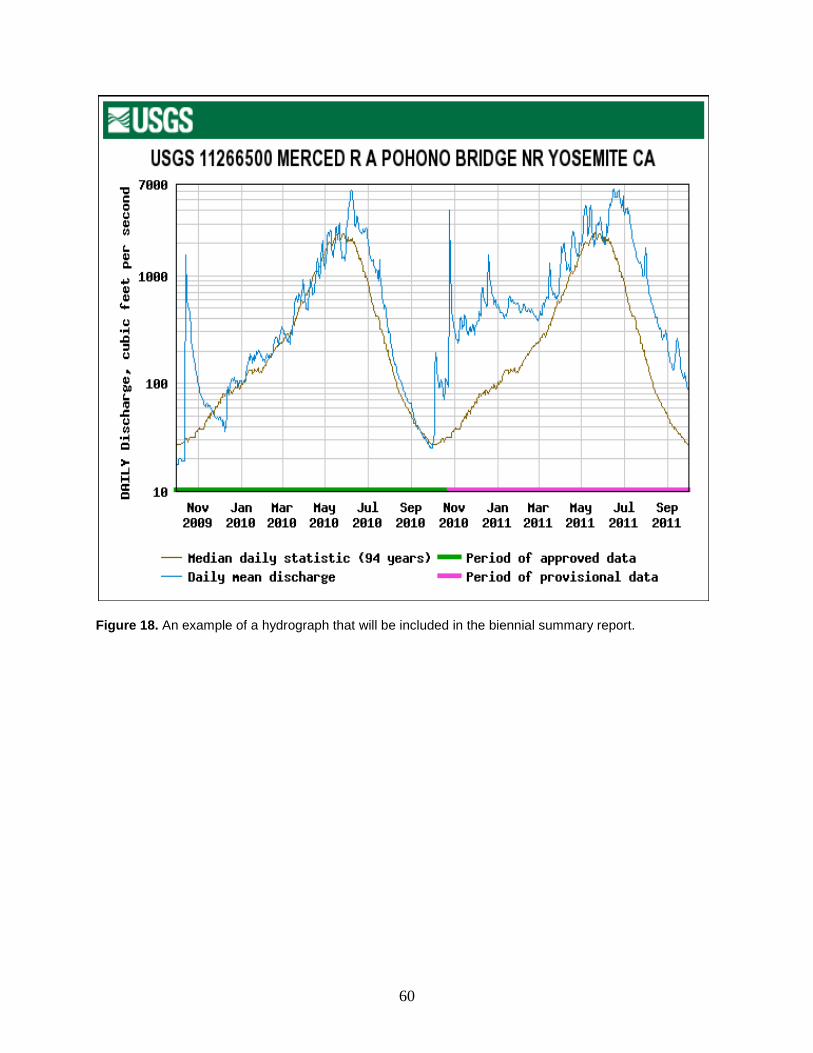
60

Figure 18. An example of a hydrograph that will be included in the biennial summary report.

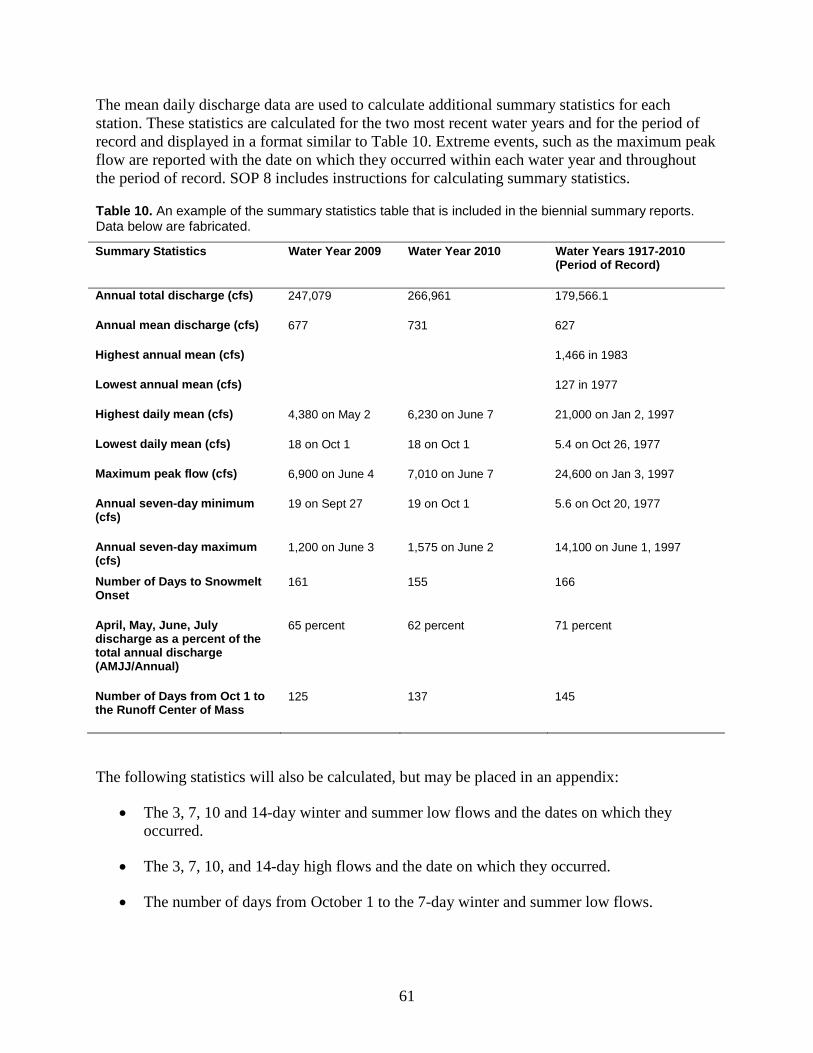
61

The mean daily discharge data are used to calculate additional summary statistics for each station. These statistics are calculated for the two most recent water years and for the period of record and displayed in a format similar to Table 10. Extreme events, such as the maximum peak flow are reported with the date on which they occurred within each water year and throughout the period of record. SOP 8 includes instructions for calculating summary statistics.

Table 10. An example of the summary statistics table that is included in the biennial summary reports. Data below are fabricated.

Summary Statistics Water Year 2009 Water Year 2010 Water Years 1917-2010 (Period of Record)

Annual total discharge (cfs) 247,079 266,961 179,566.1

Annual mean discharge (cfs) 677 731 627

Highest annual mean (cfs) 1,466 in 1983

Lowest annual mean (cfs) 127 in 1977

Highest daily mean (cfs) 4,380 on May 2 6,230 on June 7 21,000 on Jan 2, 1997

Lowest daily mean (cfs) 18 on Oct 1 18 on Oct 1 5.4 on Oct 26, 1977

Maximum peak flow (cfs) 6,900 on June 4 7,010 on June 7 24,600 on Jan 3, 1997

Annual seven-day minimum (cfs)

19 on Sept 27 19 on Oct 1 5.6 on Oct 20, 1977

Annual seven-day maximum (cfs)

1,200 on June 3 1,575 on June 2 14,100 on June 1, 1997

Number of Days to Snowmelt Onset

161 155 166

April, May, June, July discharge as a percent of the total annual discharge (AMJJ/Annual)

65 percent 62 percent 71 percent

Number of Days from Oct 1 to the Runoff Center of Mass

125 137 145

The following statistics will also be calculated, but may be placed in an appendix:

• The 3, 7, 10 and 14-day winter and summer low flows and the dates on which they occurred.

• The 3, 7, 10, and 14-day high flows and the date on which they occurred.

• The number of days from October 1 to the 7-day winter and summer low flows.

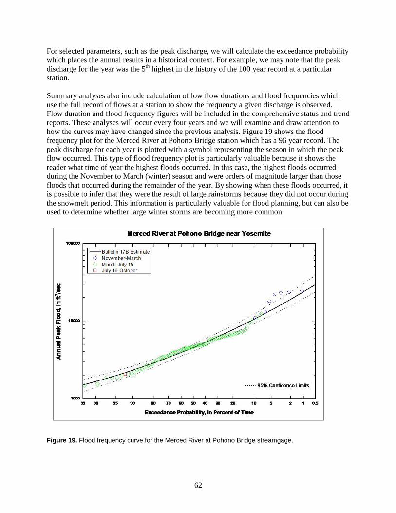
62

For selected parameters, such as the peak discharge, we will calculate the exceedance probability which places the annual results in a historical context. For example, we may note that the peak discharge for the year was the 5th highest in the history of the 100 year record at a particular station. Summary analyses also include calculation of low flow durations and flood frequencies which use the full record of flows at a station to show the frequency a given discharge is observed. Flow duration and flood frequency figures will be included in the comprehensive status and trend reports. These analyses will occur every four years and we will examine and draw attention to how the curves may have changed since the previous analysis. Figure 19 shows the flood frequency plot for the Merced River at Pohono Bridge station which has a 96 year record. The peak discharge for each year is plotted with a symbol representing the season in which the peak flow occurred. This type of flood frequency plot is particularly valuable because it shows the reader what time of year the highest floods occurred. In this case, the highest floods occurred during the November to March (winter) season and were orders of magnitude larger than those floods that occurred during the remainder of the year. By showing when these floods occurred, it is possible to infer that they were the result of large rainstorms because they did not occur during the snowmelt period. This information is particularly valuable for flood planning, but can also be used to determine whether large winter storms are becoming more common.

Figure 19. Flood frequency curve for the Merced River at Pohono Bridge streamgage.

63

6.1.2 Trend Analysis Trend analyses will be performed on the yearly hydrologic statistics that were calculated as part of the summary analyses. Andrews (2012) confirms the published findings of other broad regional studies that do not show widespread significant trends in mean annual streamflow (Luce and Holden 2009, Pagano and Garen 2005). However, stationarity in mean annual flow does not indicate stationarity in the rest of the distribution (Luce and Holden 2009). For this reason, we will examine trends in a variety of hydrologic statistics that are more descriptive of streamflow timing.

The first step in trend analysis is to plot the data that will be analyzed and visually examine it for apparent trends. While trends observed in the visual assessment step may not be statistically significant, they can provide an overview of how a parameter has changed over time. For example, if the smoothed trend lines hint that a trend has been up for 10 years and then down for 10 years, a typical monotonic trend test might conclude “no trend” (Manly 2001). This conclusion might be less helpful to a resource manager than a conclusion that might result from looking at a simple plot of values vs. time.

There are several parametric, non-parametric and mixed methods for hydrologic trend analysis. In preparation for this protocol, Starcevich and Kane (Appendix C) performed trend analyses for multiple statistics from two SIEN rivers and found that a parametric test may be significant at the 0.10 level when the nonparametric test is not significant and vice versa. For this reason and to add weight to any significant results, we will use more than one test when performing our trend analysis.

Linear regression is considered a fundamental tool in the analysis of water-resources data (Helsel and Hirsch 2002). Linear regression is the process of fitting a straight line to a data set that consists of an explanatory (independent, predictor, or X) variable and a response (dependent, predicted, or Y) variable. We will use either linear regression or the linear mixed model as described in the trend and power analysis (see Appendix C). A mixed model allows some effects to be considered fixed and some to be considered random. Fixed effects contribute to the mean of the outcome and random effects contribute to the variance. Random effects are used to estimate variation of linear trends among subjects (e.g., streams) and over time.

Although ordinary least squares regression (OLS) is a commonly used parametric method for analyzing hydrologic data, such data sets often have outliers and skewed distributions that violate the assumptions inherent in parametric statistical techniques (Hirsch et al. 1982). Thus, parametric techniques may be inappropriate for some hydrologic data sets. Helsel and Hirsch (2002) recommend the Kendall-Theil robust line as a nonparametric alternative to OLS methods for statistical analysis of water-resources data. Stahl et al. (2010) used the Kendall-Theil robust line to assess discharge trends in watersheds throughout Europe. This robust nonparametric method is resistant to the effects of outliers and non-normality in residuals that commonly characterize hydrologic data sets. The USGS has created a Visual Basic program for using the Kendall-Theil robust line (Granato 2006).

The Mann-Kendall Test (MKT) is another nonparametric statistical method used to assess trends in data sets that has been used by the USGS to assess trends at their streamgages (Lins and Slack 1999). The advantages of this test are that it is widely-used and applicable to any type of

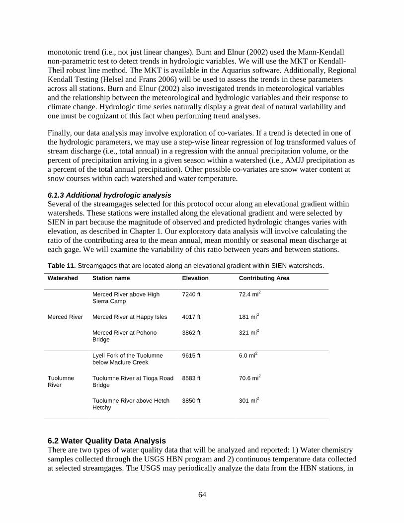
64

monotonic trend (i.e., not just linear changes). Burn and Elnur (2002) used the Mann-Kendall non-parametric test to detect trends in hydrologic variables. We will use the MKT or Kendall-Theil robust line method. The MKT is available in the Aquarius software. Additionally, Regional Kendall Testing (Helsel and Frans 2006) will be used to assess the trends in these parameters across all stations. Burn and Elnur (2002) also investigated trends in meteorological variables and the relationship between the meteorological and hydrologic variables and their response to climate change. Hydrologic time series naturally display a great deal of natural variability and one must be cognizant of this fact when performing trend analyses.

Finally, our data analysis may involve exploration of co-variates. If a trend is detected in one of the hydrologic parameters, we may use a step-wise linear regression of log transformed values of stream discharge (i.e., total annual) in a regression with the annual precipitation volume, or the percent of precipitation arriving in a given season within a watershed (i.e., AMJJ precipitation as a percent of the total annual precipitation). Other possible co-variates are snow water content at snow courses within each watershed and water temperature.

6.1.3 Additional hydrologic analysis Several of the streamgages selected for this protocol occur along an elevational gradient within watersheds. These stations were installed along the elevational gradient and were selected by SIEN in part because the magnitude of observed and predicted hydrologic changes varies with elevation, as described in Chapter 1. Our exploratory data analysis will involve calculating the ratio of the contributing area to the mean annual, mean monthly or seasonal mean discharge at each gage. We will examine the variability of this ratio between years and between stations.

Table 11. Streamgages that are located along an elevational gradient within SIEN watersheds.

Watershed Station name Elevation Contributing Area

Merced River

Merced River above High Sierra Camp

7240 ft 72.4 mi2

Merced River at Happy Isles 4017 ft 181 mi2

Merced River at Pohono Bridge

3862 ft 321 mi2

Tuolumne River

Lyell Fork of the Tuolumne below Maclure Creek

9615 ft 6.0 mi2

Tuolumne River at Tioga Road Bridge

8583 ft 70.6 mi2


3850 ft 301 mi2

6.2 Water Quality Data Analysis There are two types of water quality data that will be analyzed and reported: 1) Water chemistry samples collected through the USGS HBN program and 2) continuous temperature data collected at selected streamgages. The USGS may periodically analyze the data from the HBN stations, in

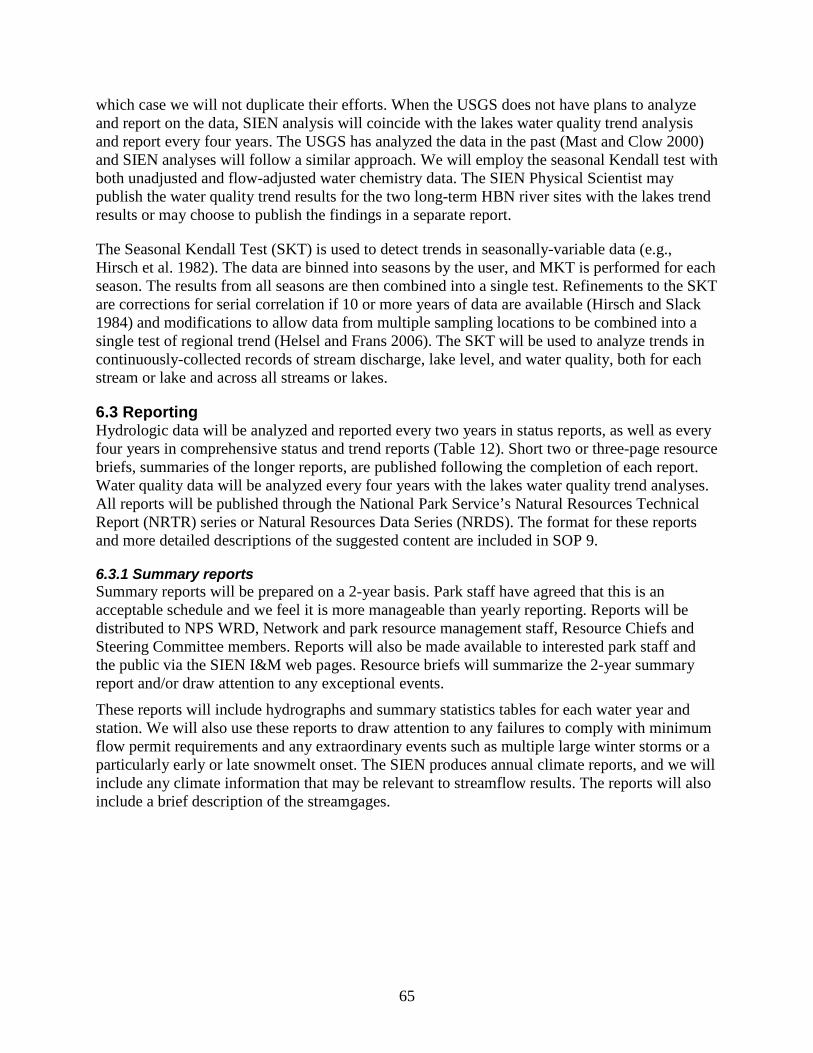
65

which case we will not duplicate their efforts. When the USGS does not have plans to analyze and report on the data, SIEN analysis will coincide with the lakes water quality trend analysis and report every four years. The USGS has analyzed the data in the past (Mast and Clow 2000) and SIEN analyses will follow a similar approach. We will employ the seasonal Kendall test with both unadjusted and flow-adjusted water chemistry data. The SIEN Physical Scientist may publish the water quality trend results for the two long-term HBN river sites with the lakes trend results or may choose to publish the findings in a separate report.

The Seasonal Kendall Test (SKT) is used to detect trends in seasonally-variable data (e.g., Hirsch et al. 1982). The data are binned into seasons by the user, and MKT is performed for each season. The results from all seasons are then combined into a single test. Refinements to the SKT are corrections for serial correlation if 10 or more years of data are available (Hirsch and Slack 1984) and modifications to allow data from multiple sampling locations to be combined into a single test of regional trend (Helsel and Frans 2006). The SKT will be used to analyze trends in continuously-collected records of stream discharge, lake level, and water quality, both for each stream or lake and across all streams or lakes.

6.3 Reporting Hydrologic data will be analyzed and reported every two years in status reports, as well as every four years in comprehensive status and trend reports (Table 12). Short two or three-page resource briefs, summaries of the longer reports, are published following the completion of each report. Water quality data will be analyzed every four years with the lakes water quality trend analyses. All reports will be published through the National Park Service’s Natural Resources Technical Report (NRTR) series or Natural Resources Data Series (NRDS). The format for these reports and more detailed descriptions of the suggested content are included in SOP 9.

6.3.1 Summary reports Summary reports will be prepared on a 2-year basis. Park staff have agreed that this is an acceptable schedule and we feel it is more manageable than yearly reporting. Reports will be distributed to NPS WRD, Network and park resource management staff, Resource Chiefs and Steering Committee members. Reports will also be made available to interested park staff and the public via the SIEN I&M web pages. Resource briefs will summarize the 2-year summary report and/or draw attention to any exceptional events.

These reports will include hydrographs and summary statistics tables for each water year and station. We will also use these reports to draw attention to any failures to comply with minimum flow permit requirements and any extraordinary events such as multiple large winter storms or a particularly early or late snowmelt onset. The SIEN produces annual climate reports, and we will include any climate information that may be relevant to streamflow results. The reports will also include a brief description of the streamgages.

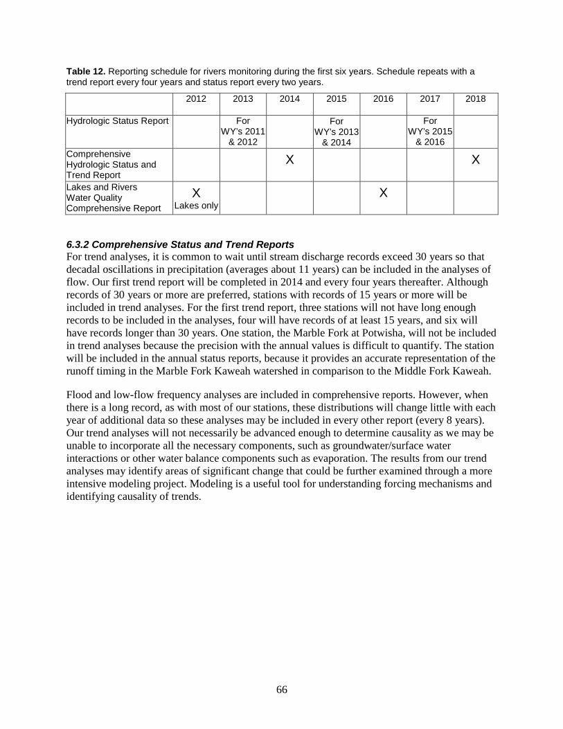
66

Table 12. Reporting schedule for rivers monitoring during the first six years. Schedule repeats with a trend report every four years and status report every two years.

2012 2013 2014 2015 2016 2017 2018

Hydrologic Status Report For WY’s 2011

& 2012

For WY’s 2013

& 2014

For WY’s 2015

& 2016

Comprehensive Hydrologic Status and Trend Report

X X

Lakes and Rivers Water Quality Comprehensive Report

X Lakes only

X

6.3.2 Comprehensive Status and Trend Reports For trend analyses, it is common to wait until stream discharge records exceed 30 years so that decadal oscillations in precipitation (averages about 11 years) can be included in the analyses of flow. Our first trend report will be completed in 2014 and every four years thereafter. Although records of 30 years or more are preferred, stations with records of 15 years or more will be included in trend analyses. For the first trend report, three stations will not have long enough records to be included in the analyses, four will have records of at least 15 years, and six will have records longer than 30 years. One station, the Marble Fork at Potwisha, will not be included in trend analyses because the precision with the annual values is difficult to quantify. The station will be included in the annual status reports, because it provides an accurate representation of the runoff timing in the Marble Fork Kaweah watershed in comparison to the Middle Fork Kaweah.

Flood and low-flow frequency analyses are included in comprehensive reports. However, when there is a long record, as with most of our stations, these distributions will change little with each year of additional data so these analyses may be included in every other report (every 8 years). Our trend analyses will not necessarily be advanced enough to determine causality as we may be unable to incorporate all the necessary components, such as groundwater/surface water interactions or other water balance components such as evaporation. The results from our trend analyses may identify areas of significant change that could be further examined through a more intensive modeling project. Modeling is a useful tool for understanding forcing mechanisms and identifying causality of trends.

67

7. Personnel Requirements and Training 7.1 Roles and Responsibilities The SIEN Physical Scientist is the protocol lead and as such, will oversee and coordinate all efforts on rivers monitoring, perform all field activities such as streamflow discharge measurements and streamgage maintenance (with occasional support from park and network staff), communicate with the station operators to acquire data each year, manage and analyze associated data, assist with agreements and contracts, and prepare reports and other products (Table 13). The SIEN Data Manager will assist with formatting of the data, transfer of tabular data to the database, and overall data management. The SIEN Program Manager will assign budgets, supervise the Protocol Lead, manage associated contracts and agreements, and review associated products. Other park or network staff will periodically assist with field work.

Table 13. Assigned staff, specific responsibilities, and time estimates for rivers monitoring.

Assigned staff and time requirement

Responsibilities

SIEN Physical Scientist 12 pay periods

• Project oversight and administration • Protocol updates and revisions • Acquire and maintain field equipment • Maintain streamgages and perform streamflow discharge

measurements and periodic level surveys • Ensure compliance with safety procedures during all field work

that SIEN leads or participates in. • Communicate with and solicit data from non-SIEN station

operators • Manage continuous stage and water chemistry data, including

rating curves, and upload to database • Maintain and archive project records • Perform data summaries and analyses. • Complete reports, metadata, and other products on schedule • Complete permitting and compliance documents

SIEN Data Manager 2 pay periods

• Consultant on data management activities • Assist with transfer of data to the Rivers Database • Facilitate check-in, review and posting of data, metadata,

reports, and other products to national databases and clearinghouses

SIEN Program Manager 2 pay periods

• Project Lead oversight • Ensure Physical Scientist has received safety training,

understands principles, & implements safety procedures • Budget and agreement administration • Consultant on all phases of protocol review and

implementation • Review reports and other products

Other SIEN staff Intermittent – 0.5 pay period

• Assist with streamgage visits

68

7.2 Annual schedule of SIEN responsibilities Table 14 provides approximate timeframes for completing office and field work associated with this protocol. While field work will be performed throughout the year, most field work occurs in the summer and fall. Certain tasks have specific timing, such as performing high flow measurements or acquiring data from the USGS in April after it has been finalized. Other tasks, such as ordering equipment or performing data analysis, can be performed more opportunistically and during periods when it is most convenient for the SIEN Physical Scientist.

Table 14. Routine field and office tasks and approximate timeframe for completion.

Action Jan Feb Mar Apr May Jun July Aug Sept Oct Nov Dec

Assist DEPO with winter site visits (once every 6 to 8 weeks)

Upload data from SIEN stations to database, perform QA/QC, update rating curves

Obtain data from other station operators, format and upload to database

Perform high flow measurements

Perform data analysis and compile status and trend reports (could occur anytime after all data has been acquired and uploaded to the database)

Perform wading measurements and site maintenance

Repair or order equipment – send current meters for calibration

7.3 Park Contributions A key component to the success of this protocol is involvement and support from park staff. Staff from YOSE and SEKI have and will continue to contribute to this project through participation in the Water Work Group. They also will assist with park-level logistical support as time permits, and provide technical support where needed. For example, YOSE staff will provide assistance with tasks such as stabilization of sites for long-term operation, assistance with compliance documents, and survey of sites. Parks also provide significant resource support by providing office and laboratory facilities.

7.4 Qualifications and Training The primary individual responsible for this protocol’s operations is the SIEN Physical Scientist. We anticipate that the individual in this position will have met the basic requirements for a GS-11 Physical Scientist which include a basic familiarity field techniques, surface water data, data management, and data analysis. Training will include: 1) field methods as outlined in Chapter 3, 2) rating curve development and use of the Aquarius software for data management and 3) data

69

analysis methods for status and trend reports. Additionally, all staff that will perform station visits will need to be familiar with all SIEN safety principles and procedures, including use of communication devices and the ability to safely navigate to backcountry stations (all SIEN stations are located adjacent to trails). The primary training methods for all field procedures will be to first read through the SOPs, watch the USGS online trainings, and then perform the duties alongside someone with experience. There are several individuals with experience in these field methods including the USGS Hydrologic Technician in charge of the YOSE streamgages, the YOSE Hydrologist, several of the seasonal YOSE Physical Science Technicians, as well as others. Additionally, the USGS periodically offers more intensive courses in streamflow data collection techniques that the Physical Scientist may attend if they are not able to obtain the desired level of training by working with another individual in the parks or network. Training for data management activities can be acquired through online training videos that are available though the Aquarius support website and the NPS Water Resources Division (WRD) and by working closely with Aquarius customer support staff and the WRD Data Manager. SOP 2 includes a list of topics that the Physical Scientist, and any other support staff, should familiarize themselves with as well as links to informational documents and training videos.

SIEN and DEPO staff will also require training on safely conducting winter streamgage visits. The USGS Hydrologist will train and advise SIEN and DEPO staff at the DEPO gage until park staff are proficient enough to perform the duties independently. The DEPO Chief Ranger will be one of the individuals performing these winter visits and will conduct a safety briefing prior to each visit with all participating staff, which will include a Green-Amber-Red risk analysis, discussion of possible hazards, and the weather forecast.

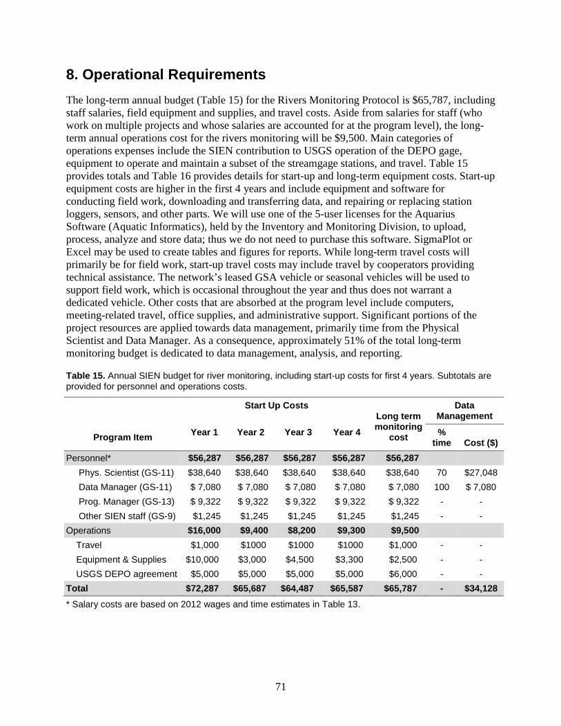
71

8. Operational Requirements The long-term annual budget (Table 15) for the Rivers Monitoring Protocol is $65,787, including staff salaries, field equipment and supplies, and travel costs. Aside from salaries for staff (who work on multiple projects and whose salaries are accounted for at the program level), the long-term annual operations cost for the rivers monitoring will be $9,500. Main categories of operations expenses include the SIEN contribution to USGS operation of the DEPO gage, equipment to operate and maintain a subset of the streamgage stations, and travel. Table 15 provides totals and Table 16 provides details for start-up and long-term equipment costs. Start-up equipment costs are higher in the first 4 years and include equipment and software for conducting field work, downloading and transferring data, and repairing or replacing station loggers, sensors, and other parts. We will use one of the 5-user licenses for the Aquarius Software (Aquatic Informatics), held by the Inventory and Monitoring Division, to upload, process, analyze and store data; thus we do not need to purchase this software. SigmaPlot or Excel may be used to create tables and figures for reports. While long-term travel costs will primarily be for field work, start-up travel costs may include travel by cooperators providing technical assistance. The network’s leased GSA vehicle or seasonal vehicles will be used to support field work, which is occasional throughout the year and thus does not warrant a dedicated vehicle. Other costs that are absorbed at the program level include computers, meeting-related travel, office supplies, and administrative support. Significant portions of the project resources are applied towards data management, primarily time from the Physical Scientist and Data Manager. As a consequence, approximately 51% of the total long-term monitoring budget is dedicated to data management, analysis, and reporting.

Table 15. Annual SIEN budget for river monitoring, including start-up costs for first 4 years. Subtotals are provided for personnel and operations costs.

Program Item

Start Up Costs Long term monitoring

cost

Data Management

Year 1 Year 2 Year 3 Year 4 % time Cost ($)

Personnel* $56,287 $56,287 $56,287 $56,287 $56,287 Phys. Scientist (GS-11) $38,640 $38,640 $38,640 $38,640 $38,640 70 $27,048 Data Manager (GS-11) $ 7,080 $ 7,080 $ 7,080 $ 7,080 $ 7,080 100 $ 7,080 Prog. Manager (GS-13) $ 9,322 $ 9,322 $ 9,322 $ 9,322 $ 9,322 - - Other SIEN staff (GS-9) $1,245 $1,245 $1,245 $1,245 $1,245 - - Operations $16,000 $9,400 $8,200 $9,300 $9,500 Travel $1,000 $1000 $1000 $1000 $1,000 - - Equipment & Supplies $10,000 $3,000 $4,500 $3,300 $2,500 - - USGS DEPO agreement $5,000 $5,000 $5,000 $5,000 $6,000 - - Total $72,287 $65,687 $64,487 $65,587 $65,787 - $34,128 * Salary costs are based on 2012 wages and time estimates in Table 13.

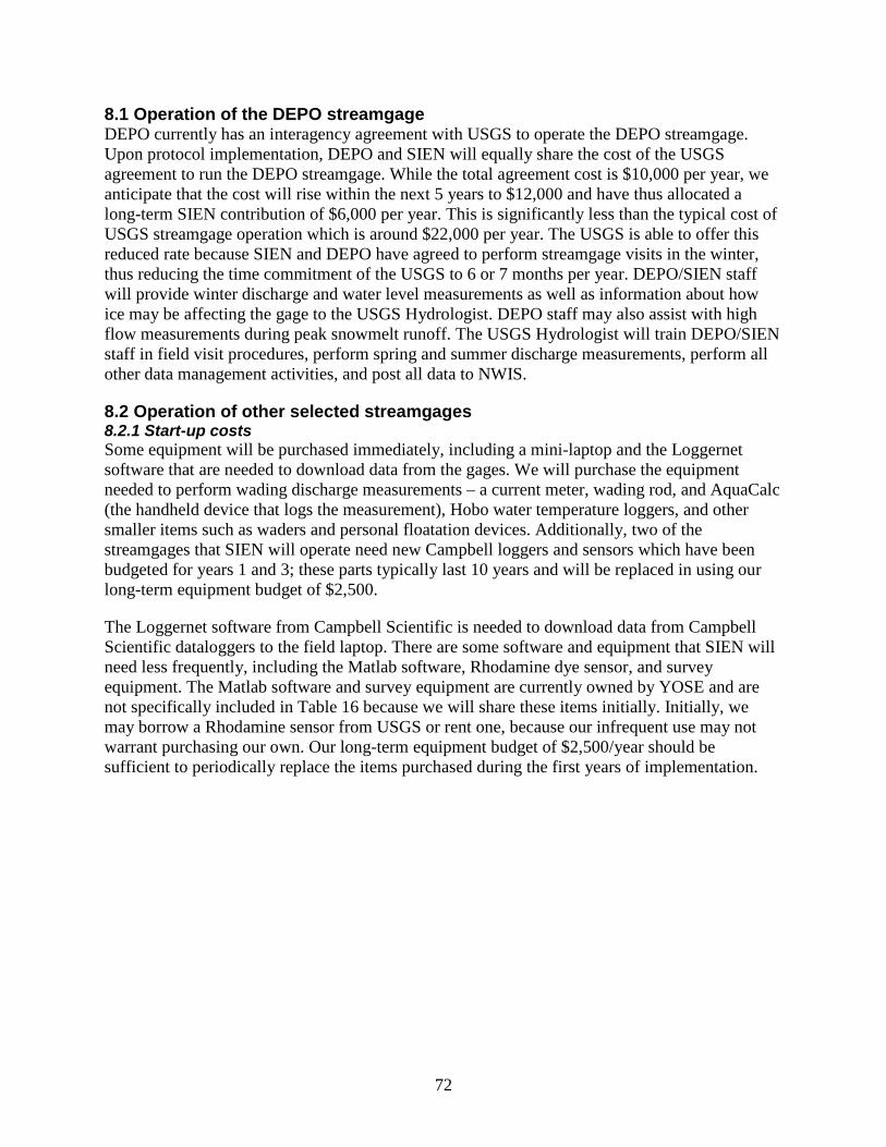
72

8.1 Operation of the DEPO streamgage DEPO currently has an interagency agreement with USGS to operate the DEPO streamgage. Upon protocol implementation, DEPO and SIEN will equally share the cost of the USGS agreement to run the DEPO streamgage. While the total agreement cost is $10,000 per year, we anticipate that the cost will rise within the next 5 years to $12,000 and have thus allocated a long-term SIEN contribution of $6,000 per year. This is significantly less than the typical cost of USGS streamgage operation which is around $22,000 per year. The USGS is able to offer this reduced rate because SIEN and DEPO have agreed to perform streamgage visits in the winter, thus reducing the time commitment of the USGS to 6 or 7 months per year. DEPO/SIEN staff will provide winter discharge and water level measurements as well as information about how ice may be affecting the gage to the USGS Hydrologist. DEPO staff may also assist with high flow measurements during peak snowmelt runoff. The USGS Hydrologist will train DEPO/SIEN staff in field visit procedures, perform spring and summer discharge measurements, perform all other data management activities, and post all data to NWIS.

8.2 Operation of other selected streamgages 8.2.1 Start-up costs Some equipment will be purchased immediately, including a mini-laptop and the Loggernet software that are needed to download data from the gages. We will purchase the equipment needed to perform wading discharge measurements – a current meter, wading rod, and AquaCalc (the handheld device that logs the measurement), Hobo water temperature loggers, and other smaller items such as waders and personal floatation devices. Additionally, two of the streamgages that SIEN will operate need new Campbell loggers and sensors which have been budgeted for years 1 and 3; these parts typically last 10 years and will be replaced in using our long-term equipment budget of $2,500.

The Loggernet software from Campbell Scientific is needed to download data from Campbell Scientific dataloggers to the field laptop. There are some software and equipment that SIEN will need less frequently, including the Matlab software, Rhodamine dye sensor, and survey equipment. The Matlab software and survey equipment are currently owned by YOSE and are not specifically included in Table 16 because we will share these items initially. Initially, we may borrow a Rhodamine sensor from USGS or rent one, because our infrequent use may not warrant purchasing our own. Our long-term equipment budget of $2,500/year should be sufficient to periodically replace the items purchased during the first years of implementation.

73

Table 16. Start-up equipment for first four years of river monitoring

Equipment and Supplies Year 1 Year 2 Year 3 Year 4 Field mini-laptop $1600 Loggernet software for downloading data from Campbell gages $600 YSI water quality meter $1400 AquaCalc, AA meter and Pygmy meter $3700 Personal Flotation Devices ($100/ea) $300 $150 Tag line tape $200 $200 Hobo Temp loggers for DEPO, SEKI and YOSE ($100/ea) $700 $300 Waders $200 $100 Replacement Campbell loggers and temperature sensors for SIEN-operated gages

$2300 $2300

Miscellaneous (Calibration solutions, NIST thermometer, etc…) $400 $100 $150 $100 Rhodamine sensor (Turner designs) – Less if cost share with YOSE

$3000

Replacement and/or repair of equipment $1500 $1500 Total $10,000 $3,000 $4,500 $3,300

8.2.2 Recurring Costs We will replace the streamgage loggers and sensors at the SIEN-operated stations during the initial years of protocol implementation and we anticipate replacement of these parts at least once every ten years. Our long-term annual equipment replacement budget is $2,500. Although equipment may not need replacing each year, we may purchase back-up equipment in years when we have excess funds.

75

9. Literature Cited

Andrews, E. D. 2012. Hydrology of the Sierra Nevada Network national parks: Status and trends. Natural Resource Report NPS/SIEN/NRR—2012/500. National Park Service, Fort Collins, Colorado.

Aquatic Informatics. 2011. Aquarius time series software: product description. Available from: http://www.aquaticinformatics.com/solutions/hydrology-environmental-analytics/flood-frequency-analysis (Accessed 10 August 2011).

Baker, V. M. Snyder, R. E. Roberts, and J. B. Martin. 2007. Rocky Mountain National Park, Nitrogen Deposition Reduction Plan. National Park Service, Environmental Protection Agency, Colorado Dept of Public Health and Environment.

Barnett, T. P., D. W. Pierce, H. G. Hidalgo, C. Bonfils, B. D. Santer, T. Das, G. Bala, A. W. Wood, T. Nozawa, A. A. Mirin, D. R. Cayan, and M. D. Dettinger. 2008. Human-induced changes in the hydrology of the western United States. Science 319:1080–1083.

Becker, A., H. Bugmann, and the IGBP (International Geosphere-Biosphere Program). 1997. Predicting global change impacts on mountain hydrology and ecology: Integrated catchment hydrology / altitudinal gradient studies. Workshop Report. IGBP-ICSU, Stockholm. Available from: http://digital.library.unt.edu/ark:/67531/metadc12000/ (Accessed 03 October, 2011)

Boiano, D. M., D. P. Weeks, and T. Hemry. 2005. Sequoia and Kings Canyon National Parks, California: Water resources information and issues overview report. Technical Report NPS/NRWRD/NRTR—2005/333, National Park Service, Denver, Colorado.

Bruns, J. A. 1998. The water quality control plan (basin plan) for the California Regional Water Quality Control Board Central Valley Region, Regional Water Quality Control Board, Central Valley Region. Sacramento, California.

Bureau of Reclamation. 2011. Reclamation, SECURE water act section 9503(c) - Reclamation climate change and water, Report to Congress, 2011. Available from: http://www.usbr.gov/climate/SECURE/docs/SECUREWaterReport.pdf (Accessed 03 August 2011).

Burn, D. H. and M. A. Elnur. 2002. Detection of hydrologic trends and variability. Journal of Hydrology 255:107-122.

Butkus, S. 2005. Quality assurance monitoring plan: streamflow gaging network. Washington State Department of Ecology. Environmental Assessment Program. Publication No. 05-03-204. Available from: http://www.ecy.wa.gov/pubs/0503204.pdf (Accessed 30 March 2010).

Cahill, T. A., J. J. Carroll, D. Campbell, and T. E. Gill. 1996. Air Quality. Pages 1227-1260 In Sierra Nevada Ecosystem Project: final report to congress, vol. II, Assessments and scientific basis for management options. University of California, Davis, California.

http://www.aquaticinformatics.com/solutions/hydrology-environmental-analytics/flood-frequency-analysis�

http://www.aquaticinformatics.com/solutions/hydrology-environmental-analytics/flood-frequency-analysis�

http://digital.library.unt.edu/ark:/67531/metadc12000/�

http://www.usbr.gov/climate/SECURE/docs/SECUREWaterReport.pdf�

http://www.ecy.wa.gov/pubs/0503204.pdf�

76

California Regional Water Quality Control Board Central Valley Region. 1995. Water quality control plan for the Tulare Lake Basin, Second Edition. Sacramento, California.

California Regional Water Quality Control Board Central Valley Region. 1998. The water quality control plan for the Sacramento River Basin and the San Joaquin River Basin, Revised September 2009. Sacramento, California.

Clow, D. W., M. A. Mast, and D. H. Campbell. 1996. Controls on surface water chemistry in the upper Merced River basin, Yosemite National Park, California. Hydrologic Processes 10:727-746.

Cook, R. R. and P. Lineback. 2008. Sierra Nevada Network data management plan. Natural Resource Report NPS/NRPC/NRR—2008/070. National Park Service, Fort Collins, Colorado.

Das, T., H. G. Hidalgo, M. D. Dettinger, D. R. Cayan, D. W. Pierce, C. Bonfils, T. P. Barnett, G. Bala, and A. Mirin. 2009. Structure and detectability of trends in hydrological measures over the western United States. Journal of Hydrometeorology 10: 871–892.

Dettinger, M. D., F. M. Ralph, T. Das, P. J. Neiman, and D. Cayan. 2011. Atmospheric rivers, floods, and the water resources of California. Water 3: 455-478.

[EPA] Environmental Protection Agency. 1997. Guidelines for preparation of the comprehensive state water quality assessments (305b) Reports and Electronic Updates: Supplement. EPA-841-B-97-002B. US Environmental Protection Agency, Washington, D.C.

Fancy, S. G. 2011. Inventory and Monitoring Program: Program Brief. Available from: http://science.nature.nps.gov/im/assets/docs/I&M_Program_Brief_6-24-2011.pdf.

Fong, D., D. Press, M. Koenen, and M. DeBlasi. 2011. San Francisco Bay Area Network (SFAN) streamflow monitoring protocol: volume 1: narrative and appendixes - version 2.92. Natural Resource Report NPS/SFAN/NRR—2011/343. National Park Service, Fort Collins, Colorado.

Gage, E. A., L. Chow, D. J. Cooper, S.A. Haultain, J.G. Holmquist, J. R. Jones, S.T. McKinney, P.E. Moore, L.S. Mutch, L. A. H. Starcevich, and H. Werner. In Prep. Wetlands ecological integrity monitoring protocol for Sierra Nevada Network national parks: version 1.4 Draft. Natural Resource Report NPS/SIEN/NRR—2009/XXX. National Park Service, Fort Collins, Colorado.

Granato, G. E. 2006. Kendall-Theil Robust Line (KTRLine—version 1.0) - A visual basic program for calculating and graphing robust nonparametric estimates of linear-regression coefficients between two continuous variables: Techniques and Methods of the U.S. Geological Survey, book 4, chap. A7, 31 p.

Hannaford, J., G. Newton, K. Stahl, and L. Tallaksen. 2011. Decadal-scale river flow variability in Europe: evidence from long hydrometric records spanning 1900-2004. Geophysical Research Abstracts. Vol. 13, EGU2011-12053.

http://science.nature.nps.gov/im/units/sien/DataManagement_Internet.cfm�

http://science.nature.nps.gov/im/assets/docs/I&M_Program_Brief_6-24-2011.pdf�

77

Heard, A. M. and J. D. Stednick. 2005. Appendix A of SIEN Lakes Monitoring Protocol: Evaluating existing water resources information in the Sierra Nevada Network for the Vital Signs Water Quality Monitoring Plan. National Park Service Unpublished Report. Three Rivers, California.

Heard, A. M., L. A. H. Starcevich, J. O. Sickman, M. G. Rose, and D. W. Schweizer. 2012. Sierra Nevada Network Lake Monitoring Protocol. Natural Resource Report NPS/SIEN/NRR—2012/XXX. National Park Service, Fort Collins, Colorado.

Helsel, D. R. and L. M. Frans. 2006. The Regional Kendall test for trend. Environmental Science and Technology 40(13):4066 - 4073. Available from: http://dx.doi.org/10.1021/es051650b (Accessed 22 November 2011).

Helsel D. R. and R. M. Hirsch. 2002. Statistical methods in water resources—Hydrologic analysis and interpretation: Techniques of Water-Resources Investigations of the U.S. Geological Survey, chap. A3, book 4, 510 p. Available from: http://pubs.usgs.gov/twri/twri4a3/ (Accessed 11 November 2011).

Herbst, D. B. 2008. Planning for the monitoring of biological effects of hydrologic changes in Sierra Nevada stream ecosystems to detect the influence of changing climate. Presentation at CEREC. Available from: http://www.wmrs.edu/projects/cerec/pdfs/Herbst1CEREC.pdf.

Higgins J. J. 2004. Introduction to modern nonparametric statistics. Brooks/Cole-Thompson Learning. Pacific Grove, California.

Hirsch, R. M., J. R. Slack, and R. A. Smith. 1982. Techniques of trend analysis for monthly water quality data. Water Resources Research 18:107-121.

Hirsch, R. M. and J. R. Slack. 1984. A nonparametric trend test for seasonal data with serial dependence: Water Resources Research 20(6): 727-732.

Interagency Climate Change Adaptation Task Force. 2011. Draft National Action Plan: Priorities for managing freshwater resources in a changing climate. Council on Environmental Quality, Washington, DC. Available from: http://www.whitehouse.gov/sites/default/files/microsites/ceq/napdraft6_2_11_final.pdf (Accessed 28 November 2011).

Intergovernmental Panel on Climate Change. 2007. Climate change 2007. IPCC Fourth Assessment Report (AR4). Available from: http://www.ipcc.ch/ (Accessed 21 November 2011).

Irwin, R. J. 2008. Draft Part B lite QA/QC review checklist for aquatic vital sign monitoring protocols and SOPs. National Park Service, Water Resources Division. Fort Collins, Colorado. Available from: http://www.nature.nps.gov/water/Vital_Signs_Guidance/Guidance_Documents/PartBLite.pdf (Accessed 12 November 2011).

http://dx.doi.org/10.1021/es051650b�

http://pubs.usgs.gov/twri/twri4a3/�

http://www.wmrs.edu/projects/cerec/pdfs/Herbst1CEREC.pdf�

http://www.whitehouse.gov/sites/default/files/microsites/ceq/napdraft6_2_11_final.pdf�

http://www.ipcc.ch/�

78

Jordan / Avent & Associates. 1984. A study to evaluate the impacts of Kaweah No. 3 hydroelectric facility on the resources of Sequoia National Park. Unpublished report.

Kaushal, S. S., G. E. Likens, N. A. Jaworski, M. L. Pace, A. M. Sides, D. Seekell, K. T. Belt, D. H. Secor, and R. L. Wingate. 2010. Rising stream and river temperatures in the United States. Frontiers in Ecology 8(9):461-466.

Kennedy, E. J. 1983. Computation of continuous records of streamflow. Chapter A13 in Techniques of water-resources investigations of the United States Geological Survey. Book 3. U.S. Geological Survey, Washington, D.C. Available from: http://www.ecy.wa.gov/programs/eap/models/usgs_twri.html (Accessed 30 March 2010).

Kennedy, E. J. 1990. Levels at Streamflow Gaging Stations. Chapter A19 in Techniques of Water Resources Investigations of the United States Geological Survey. Available from: http://pubs.usgs.gov/twri/ (accessed 22 November 2011).

Knowles, N., M. D. Dettinger, and D. R. Cayan. 2006. Trends in snowfall versus rainfall in the western United States. Journal of Climate 19:4545–4559.

Lins, H. F. and J. R. Slack. 1999. Streamflow trends in the United States: Geophysical Resource Letters 26: 227-230.

Luce, C. H. and Z. A. Holden. 2009. Declining annual streamflow distributions in the Pacific Northwest United States, 1948-2006. Geophysical Research Letters. 36:L16401.

Lundquist, J. D., D. R. Cayan and M. D. Dettinger. 2003. Meteorology and hydrology in Yosemite National Park: A sensor network application. Information Processing in Sensor Networks 2634:518-528.

Lundquist, J. D., D. R. Cayan, and M. D. Dettinger. 2004. Spring Onset in the Sierra Nevada: When is snowmelt independent of elevation. Journal of Hydrometeorology 5(4):327-342.

Manly, B. F. J. 2001. Statistics for environmental science and management. Chapman and Hall / CRC, Boca Raton, USA.

Mast, M. A. and D. W. Clow. 2000. Environmental characteristics and water-quality of Hydrologic Benchmark stations in the Western United States, U. S. Geological Survey Circular 1173-D, 115 p. Available from: http://pubs.usgs.gov/circ/circ1173/circ1173d/pdf-d/chapter03d.pdf (Accessed 2 August 2011).

Meyer, R. W. 1996. Surface-water quality-assurance plan for the California district of the U.S. Geological Survey. Open-File Report 96-618. U.S. Geological Survey, Sacramento, California.

Minshall, G. W., K. W. Cummins, R. C. Peterson, C. E. Cushing, D. A. Bruns, J. R. Sedell, and R. L. Vannote. 1985. Developments in stream ecosystem theory. Canadian Journal of Fisheries and Aquatic Science 42:1045-1055.

http://pubs.usgs.gov/twri/�

http://faculty.washington.edu/jdlund/publications/Lundquist_sensornetwork.pdf�

http://faculty.washington.edu/jdlund/publications/Lundquist_sensornetwork.pdf�

http://pubs.usgs.gov/circ/circ1173/circ1173d/pdf-d/chapter03d.pdf�

http://pubs.usgs.gov/circ/circ1173/circ1173d/pdf-d/chapter03d.pdf�

79

Mote, P., A. F. Hamlet, M. P. Clark, and D. P. Lettenmaier. 2005. Declining mountain snowpack in western North America. Bulletin of the American Meteorological Society 86:39–49.

Mutch, L. S., M. Goldin Rose, A. M. Heard, R. R. Cook, and G. L. Entsminger. 2008. Sierra Nevada Network vital signs monitoring plan. Natural Resource Report NPS/SIEN/NRR—2008/072. National Park Service, Fort Collins, Colorado.

[NPS] National Park Service. 2007. Final General Management Plan and Comprehensive River Management Plan/Environmental Impact Statement. Sequoia and Kings Canyon National Parks, Three Rivers, California.

[NPS] National Park Service. 2002. Recommendations for core water quality monitoring parameters and other key elements of the NPS vital signs program. National Park Service Freshwater Workgroup Subcommittee, August 15, 2002, Fort Collins, Colorado. http://science.nature.nps.gov/im/monitor/protocols/COREparam.doc

[NPS] National Park Service. 1998. National Parks Omnibus Management Act of 1998, Title II-National Park System Resource Inventory and Management. Available from: http://www.georgewright.org/title2text.pdf (Accessed 22 November 2011).

[NPS] National Park Service. 1992. Natural resource inventory and monitoring guidelines. NPS-75. NPS, Washington, D.C.

Null, S. E., J. H. Viers, and J. F. Mount. 2010. Hydrologic Response and Watershed Sensitivity to Climate Warming in California’s Sierra Nevada. PLoS ONE 5(4):e9932.

Pagano, T. C., and D. C. Garen, 2005: A recent increase in western US streamflow variability and persistence. Journal of Hydrometeorology 6: 172-179.

Peterson, D., R. Smith, I. Stewart, N. Knowles, C. Soulard, and S. Hager. 2005. Snowmelt discharge characteristics Sierra Nevada, California, Rep. 2005-5056, U.S. Department of the Interior U.S. Geological Survey, Reston, Virginia.

Peterson, D. L., D. G. Silsbee, and D. L. Schmoldt. 1995. A planning approach for developing inventory and monitoring programs in National Parks. NPS/NRUW/NRR—95/16. National Park Service, Fort Collins, Colorado.

Piepho, H. P. and J. O. Ogutu (2002). A simple mixed model for trend analysis in wildlife populations. Journal of Agricultural, Biological, and Environmental Statistics 7(3):350-360.

Rantz, S. E. and others. 1982. Computation of discharge. Volume 2 in Measurement and computation of streamflow. U.S. Geological Survey Water-Supply Paper 2175. U.S. Government Printing Office, Washington, D.C. Available from: http://pubs.usgs.gov/wsp/wsp2175/#pdf.

Sauer, V. B. 2002. Standards for the analysis and processing of surface-water data and information using electronic methods. US Geological Survey Water-Resources Investigations

http://science.nature.nps.gov/im/monitor/protocols/COREparam.doc�

http://www.georgewright.org/title2text.pdf�

http://pubs.usgs.gov/wsp/wsp2175/#pdf�

80

Report 01-4044. Available from: http://water.usgs.gov/osw/pubs/WRIR01-4044.pdf (accessed 12 November 2011).

Sauer, V. B. and R. W. Meyer. 1992. Determination of errors in individual discharge measurements. U.S. Geological Survey Open-File Report 92-144, Reston, Virginia.

Schertz, T .L., C. J. O. Childress, V. J. Kelly, M. S. O’Brien, and G. L. Pederson. 1998 A workbook for preparing a district quality-assurance plan for water-quality activities: U.S. Geological Survey Open-File Report 98-98.

Sequoia and Kings Canyon National Parks. 1999. Natural and Cultural Resources Management Plan. National Park Service, Three Rivers, California.

Shampine, W. J. 1993. Quality assurance and quality control in monitoring programs. Environmental Monitoring and Assessment 26:143–151.

Sierra Nevada Ecosystem Project. 1996. Chapter 8 Watershed and Aquatic Biodiversity. In Sierra Nevada Ecosystem Project, Final Report to Congress, Vol. I, Assessment Summaries and Management Strategies. UC Davis, Centers for Water and Wildland Resources, Davis, California.

Stahl, K., H. Hisdal, J. Hannaford, L. M. Tallaksen, H. A. J. van Lanen, E. Sauquet, S. Demuth, M. Fendekova, and J. Jódar. 2010. Streamflow trends in Europe: evidence from a dataset of near-natural catchments. Hydrol. Earth Syst. Sci. 14:2367-2382.

State Water Resources Control Board. 2011. Scoping Document - Nutrient Policy. August 2011. California Environmental Protection Agency, State Water Resources Control Board. Available from: http://www.waterboards.ca.gov/plans_policies/nutrients.shtml (Accessed 11 November 2011).

State Water Resources Control Board. 2002. 2002 California 305(b) report. California Environmental Protection Agency State Water Resources Control Board.

Stewart, I. T., D. R. Cayan, and M. D. Dettinger. 2005. Changes toward earlier streamflow timing across western North America. Journal of Climate 18:1136-1155.

Stewart, I. T. 2009. Changes in snowpack and snowmelt runoff for key mountain regions. Hydrologic Processes 23:78-94.

Tague, C. and A. L. Dugger. 2010. Ecohydrology and Climate Change in the Mountains of the Western USA – A Review of Research and Opportunities. Geography Compass 4(11):1648-1663.

Turnipseed, D. P., and Sauer, V. B. 2010. Discharge measurements at gaging stations: U.S. Geological Survey Techniques and Methods book 3, chap. A8, 87 p. Available from: http://pubs.usgs.gov/tm/tm3-a8/ (Accessed 22 November 2011).

http://water.usgs.gov/osw/pubs/WRIR01-4044.pdf�

http://www.waterboards.ca.gov/plans_policies/nutrients.shtml�

http://pubs.usgs.gov/tm/tm3-a8/�

81

Urquhart, N. S. and T. M. Kincaid. 1999. Designs for detecting trend from repeated surveys of ecological resources. Journal of Agricultural, Biological, and Environmental Statistics 4(4): 404-414.

[USGS] United States Geological Survey. 2006. Guidelines for the collection, preparation, and standardization of streamflow data. USGS Unpublished Report, Washington, D.C.

[USGS] United States Geological Survey. 1992. Policy Statement on Stage Accuracy. Office of Surface Water Technical Memorandum No. 93.07. Available from: http://water.usgs.gov/admin/memo/SW/sw93.07.html (Accessed 11 November 2011).

VanLeeuwen, D. M., L. W. Murray, and N. S. Urquhart. 1996. A mixed model with both fixed and random trend components across time. Journal of Agricultural, Biological, and Environmental Statistics 1(4):435-453.

Williamson, G. E., W. Dodds, T. K. Kratz, and M. A. Palmer. 2008. Lakes and streams as sentinels of environmental change in terrestrial and atmospheric processes. Frontiers in Ecology and the Environment 6(5):247-254.

http://water.usgs.gov/admin/memo/SW/sw93.07.html�

82

83

Appendix A. Important Data Sets, Monitoring Programs and Partnerships During phase I in the Vital Signs program development (Mutch et al. 2004), the SIEN physical scientist Andi Heard, compiled “Evaluating Existing Water Resources Information in the Sierra Nevada Network for the Vital Signs Water Quality Monitoring Plan” (Heard and Stednick 2005). This document is an excellent compilation of historic data sets and monitoring programs. In this appendix, we have drawn from information in the above compilation, highlighted programs relevant to this protocol, and described other programs that began after 2005.

Surface Water Ambient Monitoring Program (SWAMP) Reference Condition Monitoring Program (RCMP): SWAMP is a state-wide monitoring effort designed to assess the condition of water resources throughout California. It is administered by the State Water Board and implemented by the nine Regional Water Quality Control Boards. Funding limits monitoring to the highest priority waters where monitoring is most needed in each region. SWAMP coordinates with other monitoring efforts in order to capture additional information that will inform the program about the status of California’s waters. SWAMP developed criteria, which they encourage other monitoring programs to adhere to, so their data may be ‘SWAMP compatible’. Bio-assessment is an evaluation of the biological condition of a waterbody that uses biological surveys and other direct measurements of resident biota (macroinvertebrates, algae, diatoms) in surface waters. Data collected from bioassessments can be used to determine whether the biological health of the waterbody is what would be expected if pollution and other water quality stressors were not causing an effect. Reference conditions define the biological assemblages expected under minimal human influence and are fundamental to a bioassessment program. Surveying reference sites are necessary because they set objective and defensible benchmarks for attainment of ecological condition objectives, account for natural variation in expected biological assemblages in different physical settings across the state, and identify high quality watersheds to prioritize protection efforts. Reference program data can also be used to help define physical habitat expectations and thus, help separate physical habitat impairment from water quality impairment. To account for the large amounts of natural variation in the biology in California streams, reference sites are chosen from throughout the state. A subset of these sites must be sampled repeatedly over time to account for inter-annual variation at reference sites, and support the ongoing development and refinement of biological and physical condition indicator scoring tools (MMIs, O/E models, tiering of condition expectations). A number of sites were surveyed in the greater Kaweah Watershed (in SEQU) as reference sites for program in the summer of 2011. Program website: http://www.waterboards.ca.gov/water_issues/programs/swamp/.

Long-term Research and Monitoring in the Tokopah Watershed: Over 25 years of monitoring has been conducted at several waterbodies in the Tokopah watershed, located in the upper Marble Fork of the Kaweah River Watershed in Sequoia National Park. The Emerald Lake watershed is one of the most highly studied sub-alpine watersheds in the world. University of California, Santa Barbara leads the majority of the research including maintaining the gaging station at Emerald Lake (Sickman et al. 2003). However, multiple agencies and universities have contributed significant research and monitoring efforts, including U.S. Geological Survey, National Park Service, UC Riverside, and others. A number of studies have focused on water chemistry including acidic deposition (Tonnessen 1991) and nutrient dynamics (Sickman et al.

84

2003). Many of the studies have also examined climate, the water balance and hydrology of the watershed (Williams et al. 1993).

The Hydrologic Benchmark Network: A long-term monitoring program of the USGS, designed to study status and trends in surface water flow and water chemistry in minimally affected basins and as a benchmark against which to compare changes in flow and chemistry in developed watersheds. The SIEN has two HBN stations, the Merced River at Happy Isles in YOSE (1967-present) and the Marble Fork of the Kaweah above Tokopah Falls in SEKI (2003-present). The USGS provides support to the parks to collect 14 samples per year at these stations. Samples are collected more frequently during the peak snowmelt runoff period. The samples are analyzed at the USGS laboratory in Colorado and results are posted to the USGS NWIS website. The SIEN stations were visited by the USGS in 2011 to characterize the physical, chemical and biological integrity of the sites. Samples of algae, benthic invertebrates and fish were taken along with physical measurements of habitat, to establish a baseline condition and contribute to regional characterization tools such as indices of biological integrity (IBIs). In SEKI, the USGS was not able to visit the actual HBN site, and conducted their sampling downstream of Tokopah Falls near the Lodgepole Campground. The Yosemite Hydroclimate Network: In the early 1990s, researchers from numerous agencies and universities installed a network of sensors throughout YOSE to monitor hydrologic and climate dynamics. The network includes streamgages, groundwater wells, meteorological stations and others. While some of the hydroclimate researchers have ongoing research, many have completed their research, leaving established sites and data sets that can be built upon. USGS researcher Dave Clow established streamgages in both the Merced and Tuolumne watersheds with a focus on water quality (Clow et al. 1996, 2011).

University of California Santa Barbara, Sierra Nevada Aquatic Research Laboratory (Dave Herbst) - An early warning network for assessing the impacts of climate change on stream ecosystems of the Sierra Nevada: This project measures: 1) aquatic invertebrates including insects, molluscs, crustaceans, arachnids and annelids 2) Site data (channel geomorphology including substrate composition, depth, width, current velocity, slope, riparian cover, water chemistry, sedimentation, sinuosity, shading, algae density, particulate organic matter, and large wood debris, discharge, temperature, barometric pressure, etc). There are multiple sites in SEKI, YOSE, and the Forest Service Lands between the parks. The Sierra Nevada Research Institute (SNRI) at UC Merced (Roger Bales and Bob Rice)- Water balance & carbon cycling across the snow line in forested landscapes: The Mountain Hydrology Research Group at SNRI is performing extensive water balance studies at:

o Sequoia Field Station in Wolverton (SEKI) – The Marble Fork of the Kaweah Watershed.

o Yosemite Field Station in Wawona – Merced Watershed (YOSE).

Visitor Experience and Resource Protection Program (VERP): Yosemite National Park monitors a suite of indicators, including water quality and hydrology, to assess visitor use impacts along the Merced and Tuolumne Wild and Scenic River corridors. The program examines bacteria, nutrients and petroleum hydrocarbons in or downstream of heavy use areas (Clow et al. 2011, Yosemite National Park 2011).

85

California Department of Water Resources snow courses, snow pillows, and water level data: Data are available from sites operated by the California Department of Water Resources as well as other agencies through the California Data Exchange Center (CDEC) http://cdec.water.ca.gov/.

Kings River Experimental Watershed (KREW): The National Forests around KICA are involved in this integrated watershed study, which is part of the larger Kings River Project that is developing forest management techniques for sustainable forest ecosystems in the Sierra Nevada (Hunsaker 2007). Eight sub-watersheds have been chosen and fully instrumented to monitor ecosystem changes in this watershed-level, integrated ecosystem project for headwater streams in the Sierra Nevada.

http://cdec.water.ca.gov/�

86

Appendix A. Literature Cited Clow, D. W., M. A. Mast, & D. H. Campbell. 1996. Controls on surface water chemistry in the

upper Merced River basin, Yosemite National Park, California. Hydrological Processes 10:727–746.

Clow, D. W., R. S. Peavler, J. R. Roche, A. K. Panorska, J. M. Thomas, and S. Smith. 2011. Assessing possible visitor-use impacts on water quality in Yosemite National Park, California. Environmental Monitoring and Assessment DOI: 10.1007/s10661-011-1915-z

Heard, A. M. and J. D. Stednick. 2005. Evaluating existing water resources information in the Sierra Nevada Network for the Vital Signs Water Quality Monitoring Plan: Sierra Nevada Network Lake Monitoring Protocol Appendix A. Available from: http://science.nature.nps.gov/im/units/sien/monitoring/Lake_Protocol/Appendices/AppendixA_WaterSummary_2011.pdf (Accessed 06 March 2012).

Hunsaker, C. T. 2007. Kings River Experimental Watershed Research Study Plan. Sierra Nevada Research Center, Pacific Southwest Research Station, USDA Forest Service, Fresno, California.

Mutch, L. S., M. Rose, S. Martens, A. M. Heard, B. Moritsch, R. R. Cook, A. Esperanza, S. Haultain, and L. van Mantgem. 2004. Vital Signs Monitoring Plan: Phase 1 Report – Sierra Nevada Network. Unpublished report.

Sickman, J. O., J. M. Melack, and D. W. Clow. 2003. Evidence for nutrient enrichment of high-elevation lakes in the Sierra Nevada, California. Limnology and Oceanography 48(5):1885–1892.

Tonnessen, K. A. 1991. The Emerald Lake watershed study: Introduction and site description. Water Resources Research 27(7): 1537-1539.

Williams, M. A., A. D. Brown, and J. M. Melack. 1993. Geochemical and hydrologic controls on the composition of surface water in a high-elevation basin, Sierra Nevada, California. Limnology and Oceanography 38(4): 775-797.

Yosemite National Park. 2011. Visitor Use and Impacts Monitoring. Resource Brief. Available from: http://www.nps.gov/yose/naturescience/upload/02_Water_Quality.pdf (Accessed 11 August 2011).

http://science.nature.nps.gov/im/units/sien/monitoring/Lake_Protocol/Appendices/AppendixA_WaterSummary_2011.pdf�

http://science.nature.nps.gov/im/units/sien/monitoring/Lake_Protocol/Appendices/AppendixA_WaterSummary_2011.pdf�

http://www.nps.gov/yose/naturescience/upload/02_Water_Quality.pdf�

87

Appendix B. Recommendations for Expanded Surface Water Monitoring Below are recommendations that would improve coverage of major watersheds, increase types of data collected, facilitate data retrieval and accessibility, enhance our understanding of observed patterns in discharge, and engage citizens in surface water monitoring. While none of these are monumental undertakings, they are currently beyond SIEN’s capacity to implement.

1) Expanded streamflow monitoring in SEKI

a) ) The Kings River at Cedar Grove - The Kings River watershed makes up a significant portion of KICA, however, limited hydrologic data are available at this time. While the Kings River is a high priority for monitoring, SIEN does not have adequate expertise, experience, or equipment to operate a streamgage on such a large river and we do not presently have the funding to support an outside agency, such as the USGS, to operate a station. Fortunately, the California Department of Water Resources (CDWR) has received funding for the installation and operation of a station on the Kings River at Cedar Grove. We will include data from this station in our reporting and may assist with routine maintenance if it is installed.

b) The Marble Fork Kaweah at Potwisha – A streamgage was operated by Southern California Edison (SCE) at this location for 50 years. The streamgage was removed in 2002 based on concerns by SEKI and SCE that visitors were using the infrastructure for recreational purposes, which resulted in safety issues. Additionally, the cross-section is a poor location for a gage because it is frequently used by park visitors who construct small dams with rocks, which influence the streamflow control and rating curve. SCE has been providing a calculated value based upon discharge measurements at the power house downstream, below the Marble Fork and Middle Fork confluence. Although this calculated value will suffice to provide the park with assurance that minimum flows are being met, there is some uncertainty about the precision of these values. Error in the calculated value would likely confound our ability to detect trends with a high level of confidence. Therefore, if possible, it would be beneficial to re-install a streamgage near the former location, preferably upstream of the SCE diversion, in order to build upon the historic record for trend analyses. The SIEN does not have adequate resources to do so at this time, but would assist with data collection and station operation if the station were re-established.

2) Addition of conductivity to SIEN-operated gages - Conductivity can be a useful water quality parameter to monitor the effects of atmospheric deposition of pollutants, which is a primary resource threat and management concern in the SIEN parks. Several academic researchers have collected conductivity using sensors that are linked to the streamgage logger. Unfortunately, they have reported that SIEN surface waters are too dilute during much of the year for the sensors to operate properly. In dilute waters, conductivity sensors often have reduced precision and need to be checked or re-calibrated frequently. Water quality monitoring equipment is continually improving and there may eventually be sensors available that work well in dilute waters.

88

3) Addition of GOES satellite for real-time data transmittal to SIEN-operated gages. Real-time data transmittal is useful for several purposes. First, the operator is able to see and quickly respond to problems with the logger. Several months may pass between station visits, during which time data collection may cease due to problems with the battery or wiring. The operator can respond much more quickly to such issues and minimize the amount of data lost, if they are able to view the data in real-time. Additionally, water managers, such as the Merced Irrigation District (MID), need real-time data to respond more quickly to flood hazards. MID may be willing to provide some funding support to install a satellite at the Merced above High Sierra Camp streamgage. 3) Expanded water level monitoring throughout the SIEN– Streamgages provide both water level and discharge, but are time-consuming and costly to operate due to the necessary site visits. Water level monitoring stations do not provide discharge, but are fairly easy to install and can act as sentinels of change across the SIEN, providing information about streamflow timing, including snowmelt and thunderstorms. An expanded network of stage monitoring on tributaries to the major rivers we are already monitoring would also expand our understanding of contributions to these rivers. For example, the Illiloutte has a large percentage of its drainage area in the rain/snow transition zone. For planning purposes and to better understand climate change effects near the rain/snow transition, it would be helpful to monitor the upper Merced, Tenaya Creek and Illilouette Creek and their contributions to the lower Merced. In SEKI, water level monitoring on the major tributaries to the Kern would expand our knowledge of dynamics in this southernmost SIEN watershed where the only gage is located below most major tributaries and outside the park. To undertake installation and continued downloading of a network of water level loggers, the SIEN would need to partner with other park programs, because several of the desired locations are remote and SIEN does not have adequate staff time.

4) Continuous water quality monitoring citizen science In SEKI, the interpretation staff works with volunteers who monitor the accessible portions of the Kaweah River to increase visitor safety. The interpreters have expressed their interest in expanding the volunteer program to include water quality monitoring. SIEN could partner with the interpreters and volunteers to calibrate and cycle the continuous monitoring sondes at the Kaweah gages. Additionally, SIEN could work with volunteers to install and download data from low-cost temperature sensors (such as ibuttons) in streams throughout the SIEN. The sensors can be used to indicate when streamflow ceases. This would stimulate interest in water quality and provide SIEN with some basic water quality data.

89

Appendix C. Power Analysis of Trends in Streamflow Parameters for the Sierra Nevada Network

Version 1.0 Submitted to the Sierra Nevada Network January 2012 Revision History Log Previous Version

#

Revision date

Author Changes Justification Section and

paragraph

New Version

#

Authors:

Leigh Ann Harrod Starcevich PO Box 1032 Corvallis, OR 97339 (541) 738 6198

Stephanie L. Kane PO Box 444290 Moscow, ID 83844-4290 (208) 885 5849

Please cite this appendix as:

Starcevich, L. A. H. and S. L. Kane. 2012. Appendix C: Power analysis of trends in streamflow parameters for the Sierra Nevada Network. In Skancke, J. R., A. L. Chung-MacCoubrey, and L. Chow. 20XX. Sierra Nevada Network Rivers Monitoring Protocol: Protocol Narrative. Natural Resource Report NPS/XXXX/NRR—20XX/XXX. National Park Service, Fort Collins, Colorado.

90

Appendix C. Contents Page

Figures........................................................................................................................................... 91

Tables ............................................................................................................................................ 93

Introduction ................................................................................................................................... 94

Trend Analysis .............................................................................................................................. 94

Historic Data ..................................................................................................................... 94

Trend Methods ................................................................................................................ 102

Trend Test Results .......................................................................................................... 107

Nonparametric Test of Trends ........................................................................................ 114

Comparing the Results .................................................................................................... 115

Power Analysis ........................................................................................................................... 117

Conclusions ................................................................................................................................. 127

Literature Cited ........................................................................................................................... 128

91

Appendix C. Figures Page

Figure C.1. Kern High Flows....................................................................................................... 95

Figure C.2. Merced High Flows .................................................................................................. 95

Figure C.3. Number of days from October 1 to 3 and 14-day high flows at the Kern River ...... 96

Figure C.4. Number of days from October 1 to 3 and 14-day high flows at the Merced River .............................................................................................................................................. 96

Figure C.5. Kern Winter Low Flows ........................................................................................... 97

Figure C.6. Merced Winter Low Flows ....................................................................................... 97

Figure C.7. Kern Summer Low Flows ......................................................................................... 98

Figure C.8. Merced Summer Low Flows .................................................................................... 98

Figure C.9. Kern Days to Seasonal Low Flows ........................................................................... 99

Figure C.10. Merced Days to Seasonal Low Flows .................................................................... 99

Figure C.11. Mean Annual Flow, Kern and Merced Rivers ...................................................... 100

Figure C.12. Percent of Annual Flow from April to July, Kern and Merced Rivers................. 100

Figure C.13. Days from October 1 to Center of Mass, Kern and Merced Rivers ..................... 101

Figure C.14. Days January 1 to Onset of Snowmelt, Kern and Merced Rivers ........................ 101

Figure C.15. Power to detect trends in the three- and seven-day highs in the Kern and Merced Rivers for two levels of change and two trend tests ...................................................... 118

Figure C.16. Power to detect trends in the ten- and fourteen-day highs in the Kern and Merced Rivers for two levels of change and two trend tests ...................................................... 119

Figure C.17. Power to detect trends in the number of days to the three-day high and the number of days to the fourteen-day high in the Kern and Merced Rivers for two levels of change and two trend tests .......................................................................................................... 120

Figure C.18. Power to detect trends in the winter three- and seven-day lows in the Kern and Merced Rivers for two levels of change and two trend tests ............................................... 121

Figure C.19. Power to detect trends in the winter fourteen-day low and summer three-day lows in the Kern and Merced Rivers for two levels of change and two trend tests .................... 122

92

Figure C.20. Power to detect trends in the summer seven- and fourteen-day lows in the Kern and Merced Rivers for two levels of change and two trend tests ...................................... 123

Figure C.21. Power to detect trends in the winter seven-day lows and in the summer seven-day lows in the Kern and Merced Rivers for two levels of change and two trend tests ... 124

Figure C.22. Power to detect trends in the mean annual discharge and in the percent of total annual flow occurring between April-July period in the Kern and Merced Rivers for two levels of change and two trend tests .................................................................................... 125

Figure C.23. Power to detect trends in the number of days from October 1 to the center of mass and in the number of days from January 1 to the onset of snowmelt in the Kern and Merced Rivers for two levels of change and two trend tests ...................................................... 126

93

Appendix C. Tables Page

Table C.1: Correspondence of the R code to the linear mixed model terms. . .......................... 106

Table C.2. Transformations, fixed effects estimates, two-sided trend test results (tests significant at the 0.10 level in bold), and variance components estimates by logged outcome for the mixed model trend analysis across rivers. ........................................................ 109

Table C.3: Transformations, fixed effects estimates, two-sided trend test results (tests significant at the 0.10 level in bold), and variance components estimates by logged outcome for the ordinary least squares trend analysis by river. .................................................. 111

Table C.4: Kendall’s tau-b statistic, by river (site). Untransformed data .................................. 114

Table C.5: Comparison of p-values for trend tests by river ....................................................... 116

94

Introduction The Sierra Nevada Network (SIEN) of the National Park Service (NPS) has identified several important resources for monitoring in the Vital Signs program. SIEN rivers and streams comprise one of the systems selected for long-term monitoring. Rivers and streams are examined by collecting discharge information from streamgages. Outcomes of interest include summaries of maximum flow discharge, minimum flow discharge, and days to an event for a range of time periods and events. In this report, streamgage outcomes from long-term data sets from the Kern and Merced Rivers are used to assess the power to detect trends in those rivers. Status, trend, and variance component estimates from the long-term data are used to conduct a power analysis Trend Analysis The historic data from the Kern and Merced Rivers are first examined. Then tests of trend are discussed and applied to the long-term data sets. The estimates of status, trend, and variance are used to inform a power analysis for trend detection.

Historic data

The available pilot data consist of daily discharge data measured in cubic feet per second (cfs) collected from streamgages in the Kern and Merced Rivers in the SIEN, California (USGS National Water Information System 2011). The Kern River has been monitored since 1913 and the Merced River has been monitored since 1916. The Kern River gage is operated by the electric company Southern California Edison (SCE), with the records reviewed and made public by the USGS while the Merced River gage is operated by the USGS. The contributing surface area for the Kern River gage is 846 mi2 and 181 mi2 for the Merced. For each river, the following 18 dependent variables were calculated (Andrews 2012):

• mean annual discharge, • 3, 7, 10, and 14-day high flow; • number of days from October 1 to three-day high flow; • number of days from October 1 to fourteen-day high flow; • 3, 7, and 14-day winter low flow; • 3, 7, and 14-day summer low flow; • number days from October 1 to winter seven-day low flow; • number of days from October 1 to summer seven-day low flow; • number of days from October 1 to the center of mass; • percent of annual flow from April to July; and • number of days from January 1 to the onset of snowmelt.

These data are provided in a command that may be used in the R programming language (2011) for analysis (Appendix A). The power to detect trend in these metrics with parametric and nonparametric approaches is examined in this report. Plots indicate that some of the metrics have substantial year-to-year variation which can differ between rivers (Figures C.1-C.14).

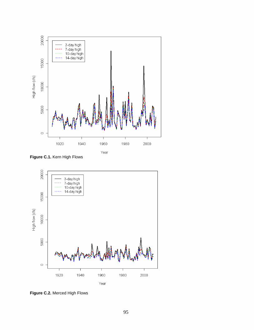
95

Figure C.1. Kern High Flows

Figure C.2. Merced High Flows

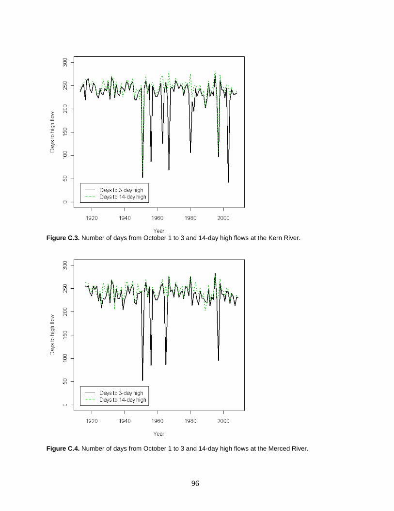
96

Figure C.3. Number of days from October 1 to 3 and 14-day high flows at the Kern River.

Figure C.4. Number of days from October 1 to 3 and 14-day high flows at the Merced River.

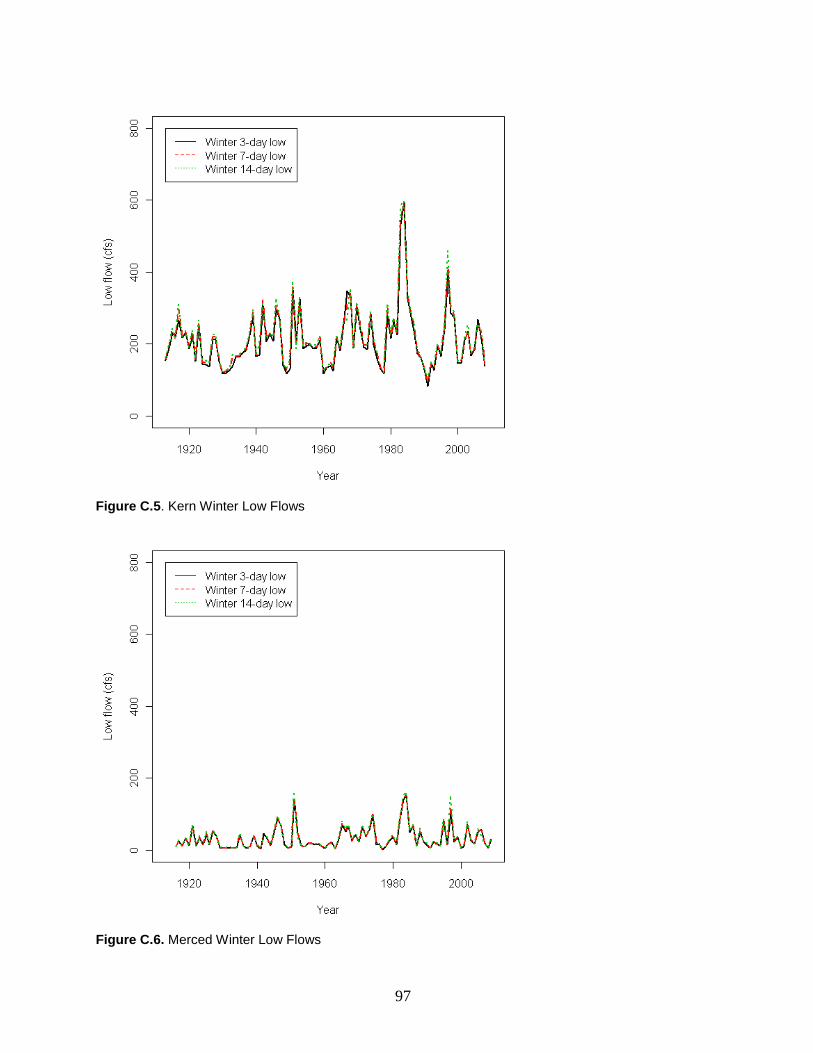
97

Figure C.5. Kern Winter Low Flows

Figure C.6. Merced Winter Low Flows

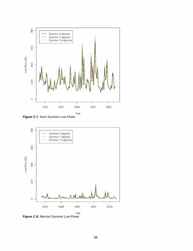
98

Figure C.7. Kern Summer Low Flows

Figure C.8. Merced Summer Low Flows

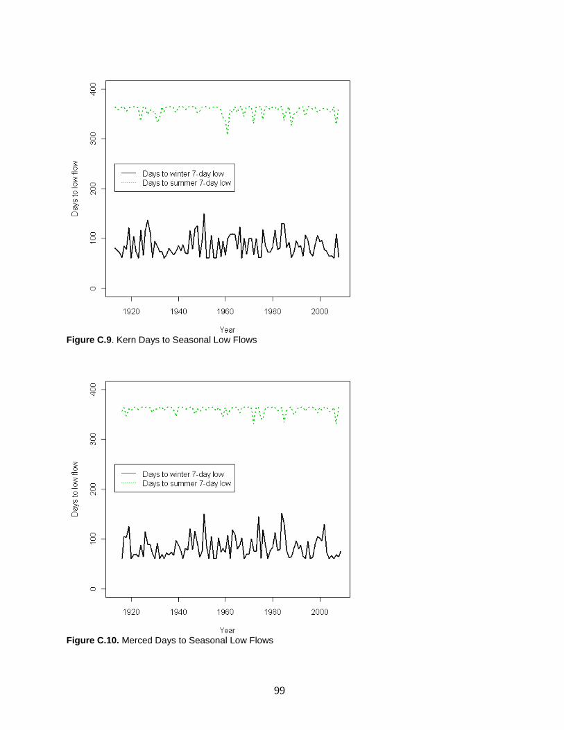
99

Figure C.9. Kern Days to Seasonal Low Flows

Figure C.10. Merced Days to Seasonal Low Flows

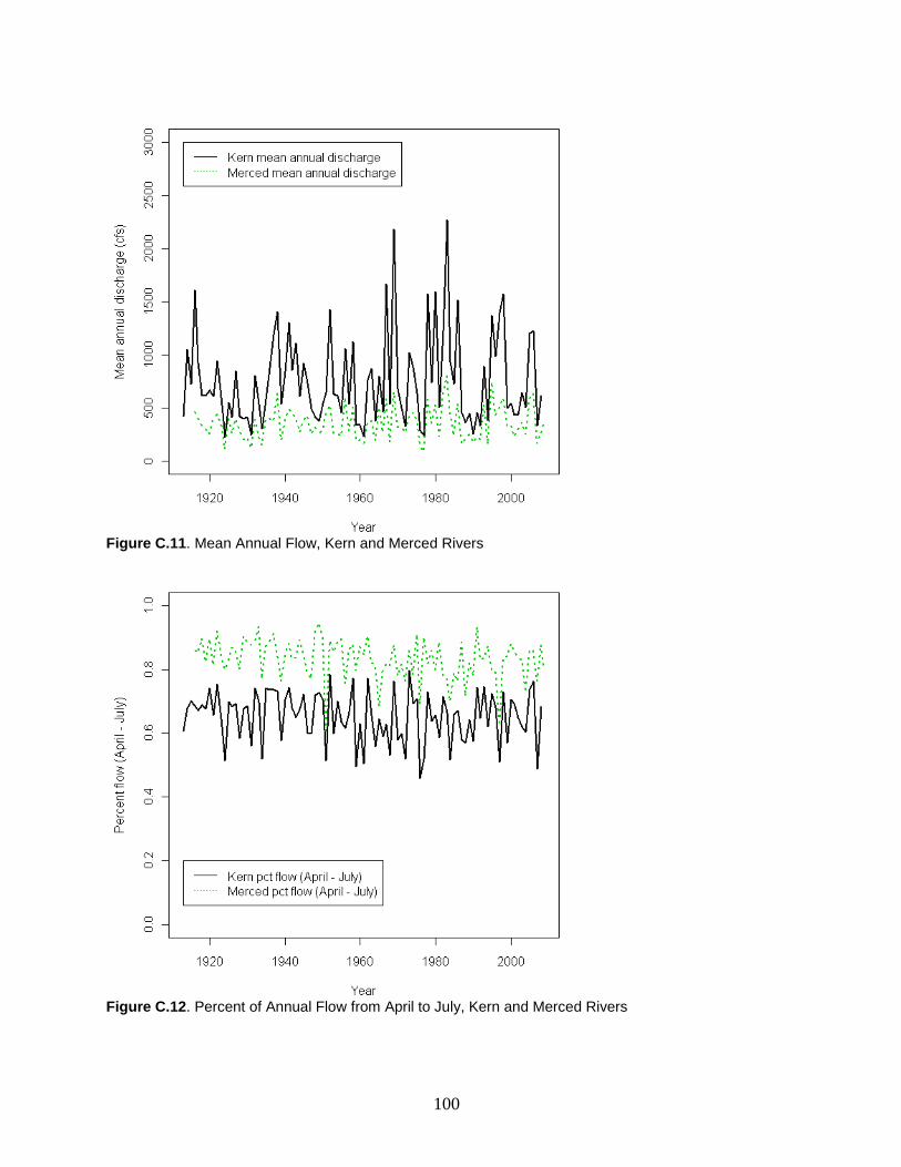
100

Figure C.11. Mean Annual Flow, Kern and Merced Rivers

Figure C.12. Percent of Annual Flow from April to July, Kern and Merced Rivers

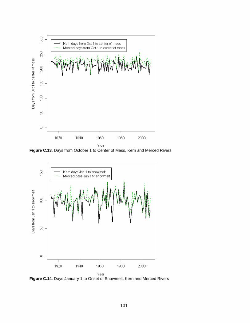
101

Figure C.13. Days from October 1 to Center of Mass, Kern and Merced Rivers

Figure C.14. Days January 1 to Onset of Snowmelt, Kern and Merced Rivers

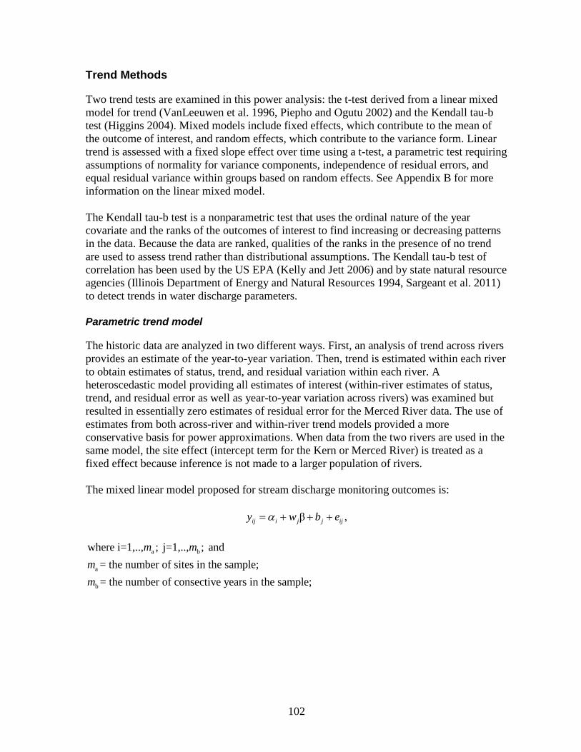
102

Trend Methods

Two trend tests are examined in this power analysis: the t-test derived from a linear mixed model for trend (VanLeeuwen et al. 1996, Piepho and Ogutu 2002) and the Kendall tau-b test (Higgins 2004). Mixed models include fixed effects, which contribute to the mean of the outcome of interest, and random effects, which contribute to the variance form. Linear trend is assessed with a fixed slope effect over time using a t-test, a parametric test requiring assumptions of normality for variance components, independence of residual errors, and equal residual variance within groups based on random effects. See Appendix B for more information on the linear mixed model. The Kendall tau-b test is a nonparametric test that uses the ordinal nature of the year covariate and the ranks of the outcomes of interest to find increasing or decreasing patterns in the data. Because the data are ranked, qualities of the ranks in the presence of no trend are used to assess trend rather than distributional assumptions. The Kendall tau-b test of correlation has been used by the US EPA (Kelly and Jett 2006) and by state natural resource agencies (Illinois Department of Energy and Natural Resources 1994, Sargeant et al. 2011) to detect trends in water discharge parameters. Parametric trend model

The historic data are analyzed in two different ways. First, an analysis of trend across rivers provides an estimate of the year-to-year variation. Then, trend is estimated within each river to obtain estimates of status, trend, and residual variation within each river. A heteroscedastic model providing all estimates of interest (within-river estimates of status, trend, and residual error as well as year-to-year variation across rivers) was examined but resulted in essentially zero estimates of residual error for the Merced River data. The use of estimates from both across-river and within-river trend models provided a more conservative basis for power approximations. When data from the two rivers are used in the same model, the site effect (intercept term for the Kern or Merced River) is treated as a fixed effect because inference is not made to a larger population of rivers. The mixed linear model proposed for stream discharge monitoring outcomes is:

β ,ij i j j ijy w b eα= + + +

a b

a

b

where i=1,.., ; j=1,.., ; and= the number of sites in the sample;= the number of consective years in the sample;

m mmm

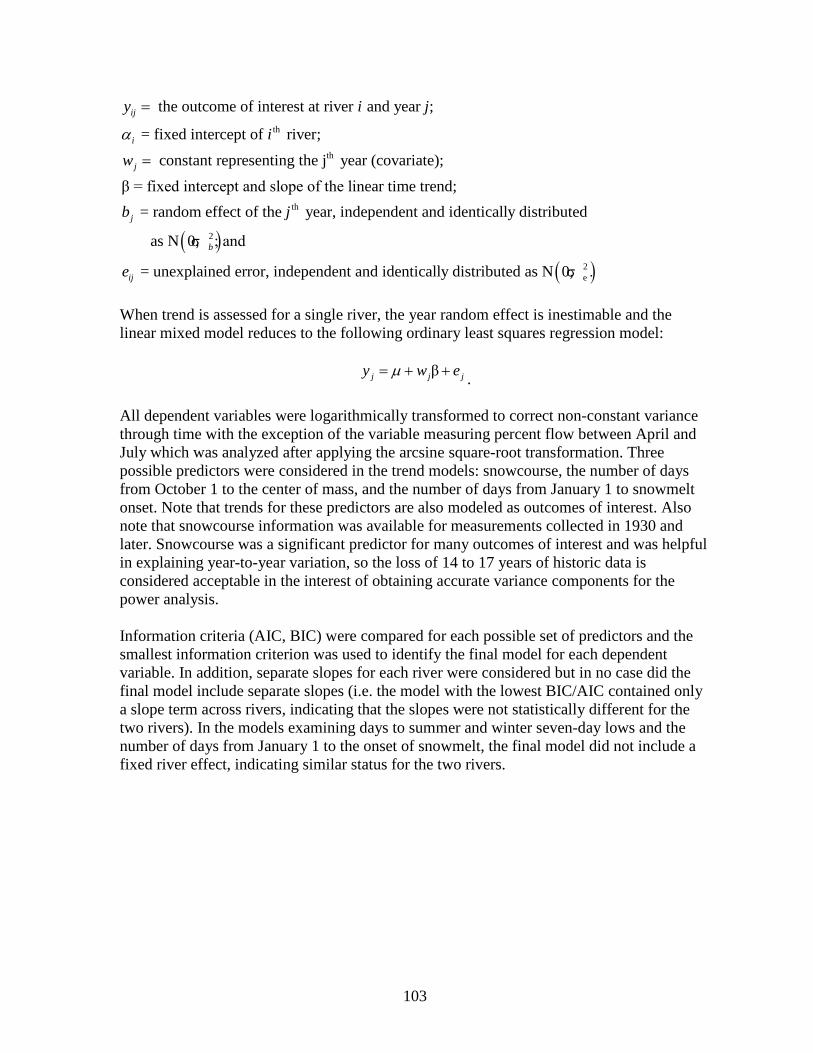
103

th

th

the outcome of interest at river and year ;

= fixed intercept of river;

constant representing the j year (covariate);

β = fixed intercept and slope of the linear time trend; = rand

ij

i

j

j

y i j

iw

b

α

=

=

( )( )

th

2

2e

om effect of the year, independent and identically distributed

as N 0,σ ; and

= unexplained error, independent and identically distributed as N 0,σ .

b

ij

j

e

When trend is assessed for a single river, the year random effect is inestimable and the linear mixed model reduces to the following ordinary least squares regression model:

βj j jy w eµ= + + .

All dependent variables were logarithmically transformed to correct non-constant variance through time with the exception of the variable measuring percent flow between April and July which was analyzed after applying the arcsine square-root transformation. Three possible predictors were considered in the trend models: snowcourse, the number of days from October 1 to the center of mass, and the number of days from January 1 to snowmelt onset. Note that trends for these predictors are also modeled as outcomes of interest. Also note that snowcourse information was available for measurements collected in 1930 and later. Snowcourse was a significant predictor for many outcomes of interest and was helpful in explaining year-to-year variation, so the loss of 14 to 17 years of historic data is considered acceptable in the interest of obtaining accurate variance components for the power analysis. Information criteria (AIC, BIC) were compared for each possible set of predictors and the smallest information criterion was used to identify the final model for each dependent variable. In addition, separate slopes for each river were considered but in no case did the final model include separate slopes (i.e. the model with the lowest BIC/AIC contained only a slope term across rivers, indicating that the slopes were not statistically different for the two rivers). In the models examining days to summer and winter seven-day lows and the number of days from January 1 to the onset of snowmelt, the final model did not include a fixed river effect, indicating similar status for the two rivers.

104

Nonparametric trend model

In addition to fitting parametric mixed models, the Kendall’s tau-b test (Higgins 2004) was used to examine linear effects of time. The Kendall tau-b is a nonparametric test to measure correlations between two variables providing an indicator of the degree of concordance or discordance where:

𝑟𝜏 =2(∑ 𝑉𝑖𝑛−1

𝑖=1 )

�𝑛2�− 1

and Vi is the number of pairs that are concordant (Higgins 2004). Large-sample properties of the test statistic are then used to evaluate the test. Like all correlation coefficients, the tau-b statistic ranges from -1 to 1. In this test, the correlation between years and the ranks of the outcome of interest is assessed. If the outcome of interest is increasing linearly over time, the ranks of the outcomes would be similar to 1, 2, 3,..., n (with a ranking of 1 given to the smallest value of the outcome). The correlation between these ranks and the year variable (1913, 1914, 1915,..,2008) would be near 1 (positively correlated). If the outcomes were decreasing over time, the ranks would be similar to n, n-1, ..., 1 and the correlation of these ranks would be near -1 (negatively correlated). A significant result for a two-sided test would be a test statistic near -1 or 1, indicating consistent change in one direction. The enhanced version of the Kendall tau-b test provides estimates of trend based on the Sen (1968) slope. Note that two variables can have very high linear correlation but very different trends. Correlation quantifies the degree but not the magnitude of the linear relationship. When the assumptions of the linear mixed model are met (see Appendix B for more on assumptions), the test of trend from the linear mixed model will tend to be more powerful than the trend test from nonparametric approaches. When the assumptions of the linear mixed model are not met, the nonparametric approach will provide the more powerful and robust trend test. If one test indicates a significant trend, it is prudent to be sure that multiple tests of trend indicate the same result before implementing an expensive management action. Explanation of the linear mixed model

An effect describes the amount by which a treatment changes the value of a measurement on a sampled unit (Kuehl 1994). A linear mixed model incorporates both fixed effects and random effects. Fixed effects are population-level effects that do not change under repeated sampling (Pinheiro and Bates, 2004). Random effects are effects associated with sampling units and may vary for repeated sampling. This variability is modeled by defining the effect as a random variable with a known distribution. The linear mixed model used in the trend analysis for both rivers is given by:

β ,ij i j j ijy w b eα= + + +

105

a b

a

b

th

where i=1,.., ; j=1,.., ; = the number of rivers in the sample;= the number of consective years in the sample;

outcome of interest (possibly transformed),

constant representing the j yij

j

m mmmy

w

=

=

( )th 2 2

ear (covariate);

= fixed intercept for river i;β = fixed slope for the linear time trend for the linear mixed model;

= random effect of the j year, iid N 0,σ , where σ is the year-to-year vari

i

j b bb

α

( )2 2e

ation; and

= unexplained error, iid as N 0,σ , where σ is the unexplained residual variation.ij ee

The random effect ( )jb is assumed to follow a normal distribution with a mean of 0 and

variance of 2σb . The expected values of the random effects are 0, so these effects do not affect the mean structure of the outcome of interest. Because these effects are assumed to be random variables that represent a larger population, the variance of the random effect impacts the variance of the outcome of interest. However, the definition of sources of variation can be informative and reduces the unexplained variation, which negatively impacts the power to detect trend. For comparison, the simple linear regression model has the form of a straight line with residual error for each observation and is given by the following notation:

ij i j ijy w eα β′ ′ ′= + + ,

( )1

2 2

= fixed river-level intercept and = slope of the linear time trend for the simple linear regression model; and

= unexplained error, iid as N 0,σ , where σ is the unexplained residual varia

i

ije

αβ′′

′ tion.

Note that the regression parameters are augmented by prime notation to distinguish these values from the regression parameters in the linear mixed model. The mean structure is defined by the fixed effects only for both the simple linear regression model ( )1and iα β′ ′ and the linear mixed model ( )1 and iα β . These parameters are not assumed to come from some larger population of effects and therefore do not affect the variance structure of the outcome of interest. For the linear mixed model, the error term is broken into a linear combination of random effects and a residual error term. The random effects correspond to components of variance for levels of factors that influence the variance structure but not the mean structure. Previous work in trend modeling (Urquhart et al., 1993; Piepho and Ogutu, 2002) has incorporated variance components for year-to-year variation ( )2

bσ , site-to-site variation ( )2aσ ,

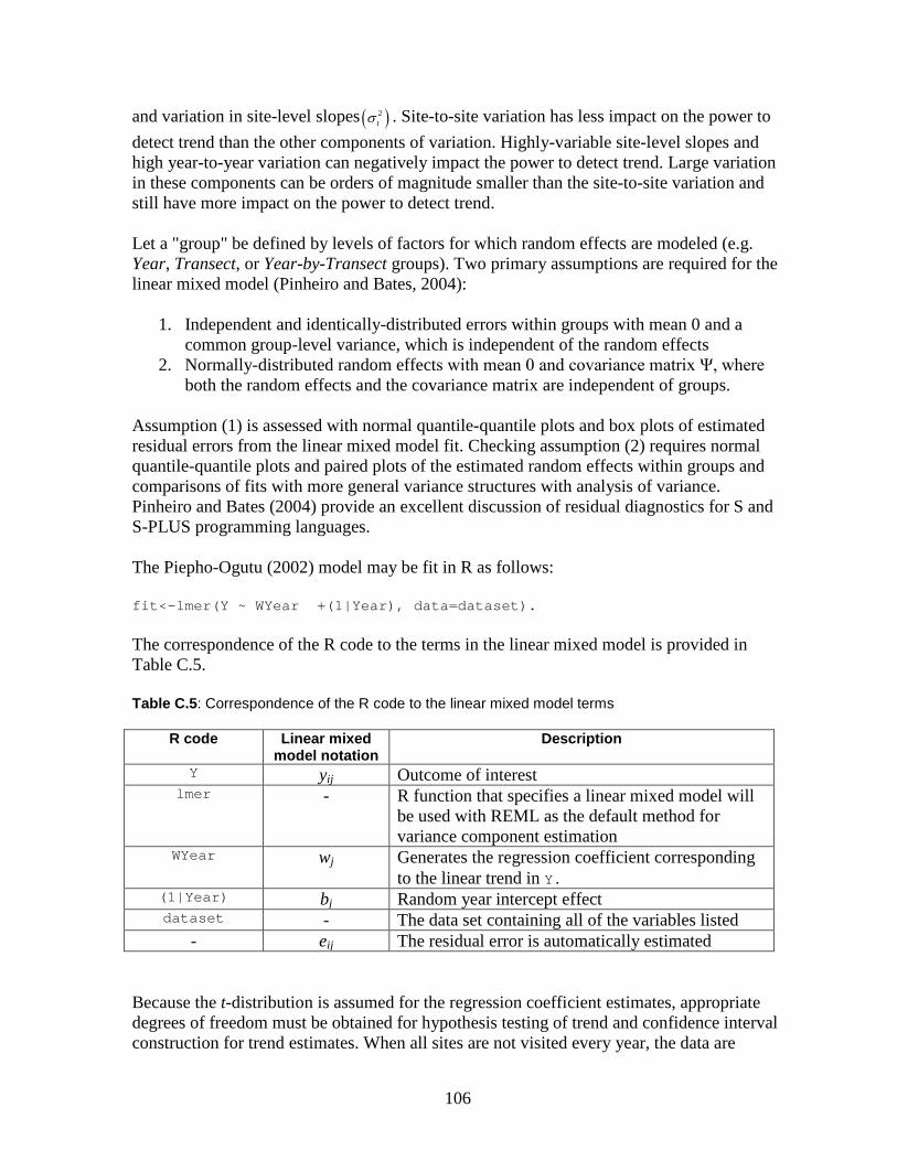
106

and variation in site-level slopes ( )2tσ . Site-to-site variation has less impact on the power to

detect trend than the other components of variation. Highly-variable site-level slopes and high year-to-year variation can negatively impact the power to detect trend. Large variation in these components can be orders of magnitude smaller than the site-to-site variation and still have more impact on the power to detect trend. Let a "group" be defined by levels of factors for which random effects are modeled (e.g. Year, Transect, or Year-by-Transect groups). Two primary assumptions are required for the linear mixed model (Pinheiro and Bates, 2004):

1. Independent and identically-distributed errors within groups with mean 0 and a common group-level variance, which is independent of the random effects

2. Normally-distributed random effects with mean 0 and covariance matrix Ψ, where both the random effects and the covariance matrix are independent of groups.

Assumption (1) is assessed with normal quantile-quantile plots and box plots of estimated residual errors from the linear mixed model fit. Checking assumption (2) requires normal quantile-quantile plots and paired plots of the estimated random effects within groups and comparisons of fits with more general variance structures with analysis of variance. Pinheiro and Bates (2004) provide an excellent discussion of residual diagnostics for S and S-PLUS programming languages. The Piepho-Ogutu (2002) model may be fit in R as follows: fit<-lmer(Y ~ WYear +(1|Year), data=dataset). The correspondence of the R code to the terms in the linear mixed model is provided in Table C.5. Table C.5: Correspondence of the R code to the linear mixed model terms

R code Linear mixed model notation

Description

Y yij Outcome of interest lmer - R function that specifies a linear mixed model will

be used with REML as the default method for variance component estimation

WYear wj Generates the regression coefficient corresponding to the linear trend in Y.

(1|Year) bj Random year intercept effect dataset - The data set containing all of the variables listed

- eij The residual error is automatically estimated Because the t-distribution is assumed for the regression coefficient estimates, appropriate degrees of freedom must be obtained for hypothesis testing of trend and confidence interval construction for trend estimates. When all sites are not visited every year, the data are

107

considered unbalanced. Sattherthwaite degrees of freedom are recommended for unbalanced data sets (Spilke et al., 2005). However, due to disagreement by R programming language developers regarding a one-size-fits-all approach to estimating degrees of freedom (see https://stat.ethz.ch/pipermail/r-help/2006-May/094765.html for more on this discussion), the degrees of freedom are not provided in lmer output. Spilke et al. (2005) recommend the Kenward-Roger (1997) degrees of freedom approximation to Satterthwaite's (1946) degrees of freedom. These may be obtained from the doBy R package.

Trend Test Results

The results of the parametric and nonparametric trend tests are discussed and compared. Two-sided trend tests are assessed at a Type I error level of 0.10. Mixed Model

When both sites are included in the trend model, significant trends are observed for ten-day high flows (p = 0.0819) and fourteen-day high flows (p = 0.0538). Statistically-significant linear trends for winter three-day low flows (p = 0.0894), winter seven-day low flows (p = 0.0960), and winter fourteen-day low flows (p = 0.0813) are also detected. The hypothesis of different slopes was rejected for every dependent variable tested, indicating that the trend for each river was not statistically different. However, the fixed effect for the river was statistically significant in every model except that for the number of days to three-day high flow (Table C.1). This indicates similar trends over time despite significantly different status estimates for most outcomes. Model selection with information criteria resulted in models containing all three potential predictors in the trend models for overall high metrics and most winter low metrics. The number of days from October 1 to the center of mass was the only predictor in the trend models for the number of days to the three-day high, the number of days to the fourteen-day high, and the number of days to the winter low. Snowcourse was the only predictor in the models of summer lows and the number of days to the summer low flow. OLS Model

Plots of the metrics over time indicated that the residual variation may differ between rivers. Therefore, the trend analyses were conducted separately for the two rivers with ordinary least squares regression since the random time effect is inestimable for a single river. Model selection employed AIC and BIC to identify suitable covariates for each trend model. Model predictors were similar between the models for each river. Snowcourse and the number of days from January 1 to the snowmelt onset were selected by model criteria to predict overall high metrics, most summer low metrics, and mean annual discharge. The number of days from October 1 to the center of mass was selected as a predictor in the trend models for the days to the three-day high for the Merced River, the days to the fourteen-day high for both rivers, and percent of variable flow from April to July for both rivers. All three predictors were retained in the models for winter lows for both rivers. The models for the number of days to the winter seven-day low and the number of days from January 1 to

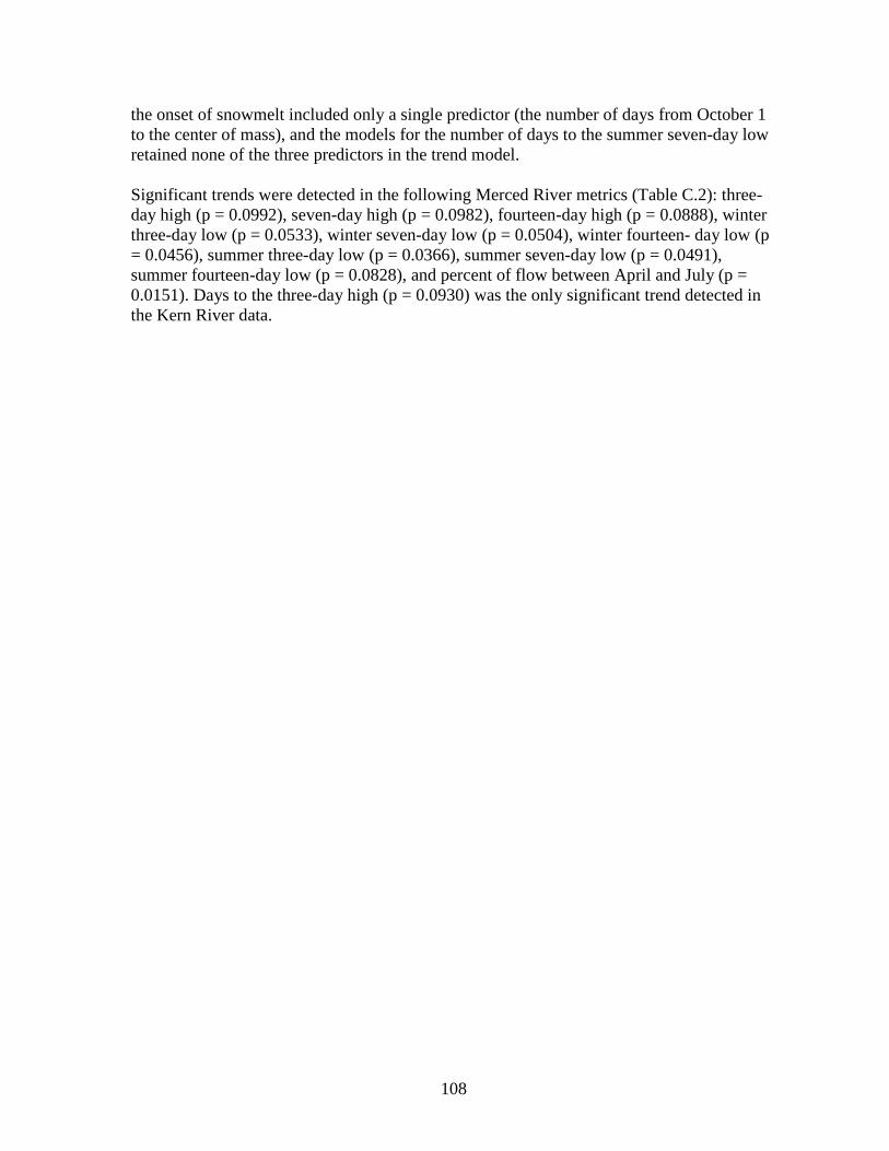
https://stat.ethz.ch/pipermail/r-help/2006-May/094765.html�

108

the onset of snowmelt included only a single predictor (the number of days from October 1 to the center of mass), and the models for the number of days to the summer seven-day low retained none of the three predictors in the trend model. Significant trends were detected in the following Merced River metrics (Table C.2): three-day high (p = 0.0992), seven-day high (p = 0.0982), fourteen-day high (p = 0.0888), winter three-day low (p = 0.0533), winter seven-day low (p = 0.0504), winter fourteen- day low (p = 0.0456), summer three-day low (p = 0.0366), summer seven-day low (p = 0.0491), summer fourteen-day low (p = 0.0828), and percent of flow between April and July (p = 0.0151). Days to the three-day high (p = 0.0930) was the only significant trend detected in the Kern River data.

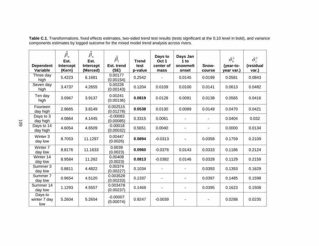
109

Table C.1. Transformations, fixed effects estimates, two-sided trend test results (tests significant at the 0.10 level in bold), and variance components estimates by logged outcome for the mixed model trend analysis across rivers.

Dependent Variable

ôβ

Est. Intercept

(Kern)

ôβ

Est. Intercept (Merced)

1̂β Est. trend

(SE)

Trend test

p-value

Days to Oct 1

center of mass

Days Jan 1 to

snowmelt onset

Snow-course

2ˆbσ (year-to-year var.)

2êσ (residual

var.) Three day

high 5.4223 6.1681 0.00177 (0.00154) 0.2542 - 0.0145 0.0199 0.0581 0.0843

Seven day high 3.4737 4.2655 0.00226

(0.00143) 0.1204 0.0109 0.0100 0.0141 0.0613 0.0482

Ten day high 3.0967 3.9137 0.00241

(0.00136) 0.0819 0.0128 0.0091 0.0138 0.0565 0.0416

Fourteen day high 2.9665 3.8149 0.002515

(0.01278) 0.0538 0.0130 0.0089 0.0149 0.0470 0.0421

Days to 3 day high 4.0864 4.1445 -0.00083

(0.00085) 0.3315 0.0061 - - 0.0404 0.032

Days to 14 day high 4.6054 4.6509 -0.00018

(0.00032) 0.5651 0.0040 - - 0.0000 0.0134

Winter 3 day low 8.7053 11.1297 0.00447

(0.0026) 0.0894 -0.0313 - 0.0358 0.1759 0.2109

Winter 7 day low 8.8176 11.1633 0.0039

(0.0023) 0.0960 -0.0376 0.0143 0.0333 0.1186 0.2124

Winter 14 day low 8.9584 11.262 0.00408

(0.0023) 0.0813 -0.0382 0.0146 0.0328 0.1129 0.2159

Summer 3 day low 0.8811 4.4822 0.00374

(0.00227) 0.1034 - - 0.0393 0.1353 0.1629

Summer 7 day low 0.9654 4.5120 0.003528

(0.00233) 0.1337 - - 0.0397 0.1485 0.1598

Summer 14 day low 1.1293 4.5557 0.003478

(0.00237) 0.1469 - - 0.0395 0.1623 0.1508

Days to winter 7 day

low 5.2604 5.2604 -0.00007

(0.00074) 0.9247 -0.0039 - - 0.0288 0.0235

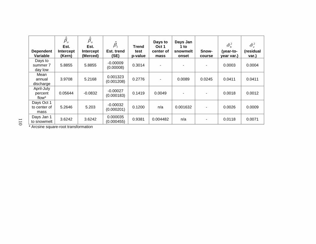
110

Dependent Variable

ôβ

Est. Intercept

(Kern)

ôβ

Est. Intercept (Merced)

1̂β Est. trend

(SE)

Trend test

p-value

Days to Oct 1

center of mass

Days Jan 1 to

snowmelt onset

Snow-course

2ˆbσ (year-to-year var.)

2êσ (residual

var.) Days to

summer 7 day low

5.8855 5.8855 -0.00009 (0.00008) 0.3014 - - - 0.0003 0.0004

Mean annual

discharge 3.9708 5.2168 0.001323

(0.001208) 0.2776 - 0.0089 0.0245 0.0411 0.0411

April-July percent

flow* 0.05644 -0.0832 -0.00027

(0.000183) 0.1419 0.0049 - - 0.0018 0.0012

Days Oct 1 to center of

mass 5.2646 5.203 -0.00032

(0.000201) 0.1200 n/a 0.001632 - 0.0026 0.0009

Days Jan 1 to snowmelt 3.6242 3.6242 0.000035

(0.000455) 0.9381 0.004482 n/a - 0.0118 0.0071

* Arcsine square-root transformation

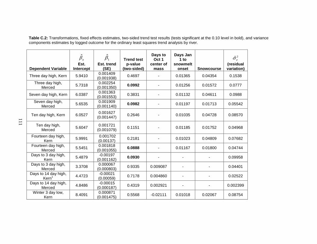
111

Table C.2: Transformations, fixed effects estimates, two-sided trend test results (tests significant at the 0.10 level in bold), and variance components estimates by logged outcome for the ordinary least squares trend analysis by river.

Dependent Variable

ôβ

Est. Intercept

1̂β Est. trend

(SE)

Trend test p-value

(two-sided)

Days to Oct 1

center of mass

Days Jan 1 to

snowmelt onset Snowcourse

2êσ (residual variation)

Three day high, Kern 5.9410 0.001409 (0.001938) 0.4697 - 0.01365 0.04354 0.1538

Three day high, Merced 5.7318 0.002254

(0.001350) 0.0992 - 0.01256 0.01572 0.0777

Seven day high, Kern 6.0387 0.001363 (0.001553) 0.3831 - 0.01132 0.04611 0.0988

Seven day high, Merced 5.6535 0.001909

(0.001140) 0.0982 - 0.01197 0.01713 0.05542

Ten day high, Kern 6.0527 0.001627 (0.001447) 0.2646 - 0.01035 0.04728 0.08570

Ten day high, Merced 5.6047 0.001721

(0.001079) 0.1151 - 0.01185 0.01752 0.04968

Fourteen day high, Kern 5.9991 0.001702

(0.00137) 0.2181 - 0.01023 0.04809 0.07682

Fourteen day high, Merced 5.5451 0.001818

(0.001055) 0.0888 - 0.01167 0.01800 0.04744

Days to 3 day high, Kern 5.4879 -0.00197

(0.001162) 0.0930 - - - 0.09958

Days to 3 day high, Merced 3.3708 0.000067

(0.000803) 0.9335 0.009087 - - 0.04401

Days to 14 day high, Kern1 4.4723 -0.00021

(0.00059) 0.7178 0.004860 - - 0.02522

Days to 14 day high, Merced 4.8486 -0.00015

(0.000187) 0.4319 0.002921 - - 0.002399

Winter 3 day low, Kern 8.4091 0.000871

(0.001475) 0.5568 -0.02111 0.01018 0.02067 0.08754

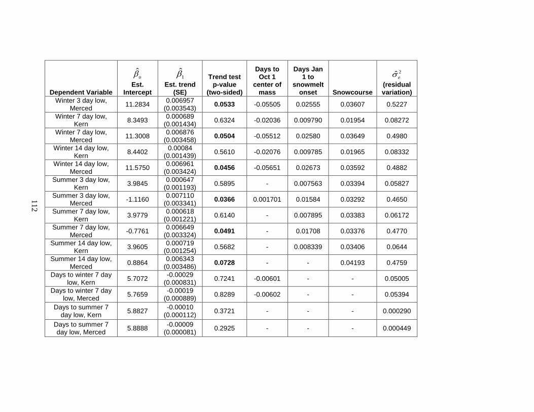
112

Dependent Variable

ôβ

Est. Intercept

1̂β Est. trend

(SE)

Trend test p-value

(two-sided)

Days to Oct 1

center of mass

Days Jan 1 to



Winter 3 day low, Merced 11.2834 0.006957

(0.003543) 0.0533 -0.05505 0.02555 0.03607 0.5227


(0.001434) 0.6324 -0.02036 0.009790 0.01954 0.08272


(0.003458) 0.0504 -0.05512 0.02580 0.03649 0.4980


(0.001439) 0.5610 -0.02076 0.009785 0.01965 0.08332


(0.003424) 0.0456 -0.05651 0.02673 0.03592 0.4882

Summer 3 day low, Kern 3.9845 0.000647

(0.001193) 0.5895 - 0.007563 0.03394 0.05827

Summer 3 day low, Merced -1.1160 0.007110

(0.003341) 0.0366 0.001701 0.01584 0.03292 0.4650


(0.001221) 0.6140 - 0.007895 0.03383 0.06172

Summer 7 day low, Merced -0.7761 0.006649

(0.003324) 0.0491 - 0.01708 0.03376 0.4770


(0.001254) 0.5682 - 0.008339 0.03406 0.0644

Summer 14 day low, Merced 0.8864 0.006343

(0.003486) 0.0728 - - 0.04193 0.4759

Days to winter 7 day low, Kern 5.7072 -0.00029

(0.000831) 0.7241 -0.00601 - - 0.05005

Days to winter 7 day low, Merced 5.7659 -0.00019

(0.000889) 0.8289 -0.00602 - - 0.05394

Days to summer 7 day low, Kern 5.8827 -0.00010

(0.000112) 0.3721 - - - 0.000290

Days to summer 7 day low, Merced 5.8888 -0.00009

(0.000081) 0.2925 - - - 0.000449

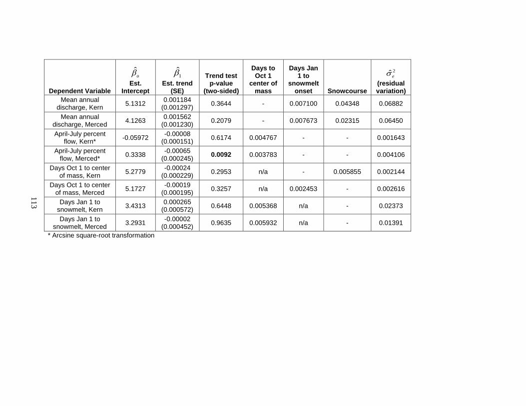
113

Dependent Variable

ôβ

Est. Intercept

1̂β Est. trend

(SE)

Trend test p-value

(two-sided)

Days to Oct 1

center of mass

Days Jan 1 to



Mean annual discharge, Kern 5.1312 0.001184

(0.001297) 0.3644 - 0.007100 0.04348 0.06882

Mean annual discharge, Merced 4.1263 0.001562

(0.001230) 0.2079 - 0.007673 0.02315 0.06450

April-July percent flow, Kern* -0.05972 -0.00008

(0.000151) 0.6174 0.004767 - - 0.001643

April-July percent flow, Merced* 0.3338 -0.00065

(0.000245) 0.0092 0.003783 - - 0.004106

Days Oct 1 to center of mass, Kern 5.2779 -0.00024

(0.000229) 0.2953 n/a - 0.005855 0.002144

Days Oct 1 to center of mass, Merced 5.1727 -0.00019

(0.000195) 0.3257 n/a 0.002453 - 0.002616

Days Jan 1 to snowmelt, Kern 3.4313 0.000265

(0.000572) 0.6448 0.005368 n/a - 0.02373

Days Jan 1 to snowmelt, Merced 3.2931 -0.00002

(0.000452) 0.9635 0.005932 n/a - 0.01391

* Arcsine square-root transformation

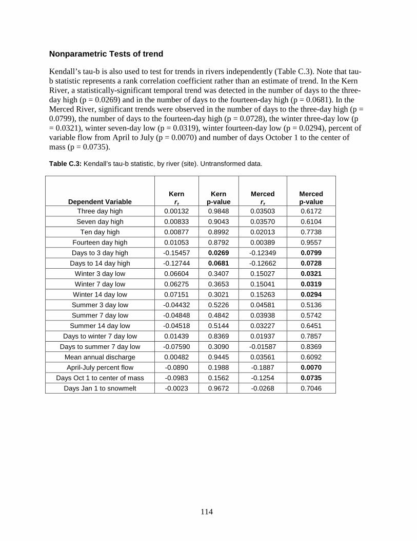
114

Nonparametric Tests of trend

Kendall’s tau-b is also used to test for trends in rivers independently (Table C.3). Note that tau-b statistic represents a rank correlation coefficient rather than an estimate of trend. In the Kern River, a statistically-significant temporal trend was detected in the number of days to the three-day high (p = 0.0269) and in the number of days to the fourteen-day high (p = 0.0681). In the Merced River, significant trends were observed in the number of days to the three-day high (p = 0.0799), the number of days to the fourteen-day high (p = 0.0728), the winter three-day low (p = 0.0321), winter seven-day low (p = 0.0319), winter fourteen-day low (p = 0.0294), percent of variable flow from April to July (p = 0.0070) and number of days October 1 to the center of mass (p = 0.0735).

Table C.3: Kendall’s tau-b statistic, by river (site). Untransformed data.

Dependent Variable Kern

rτ Kern

p-value Merced

rτ Merced p-value

Three day high 0.00132 0.9848 0.03503 0.6172 Seven day high 0.00833 0.9043 0.03570 0.6104 Ten day high 0.00877 0.8992 0.02013 0.7738

Fourteen day high 0.01053 0.8792 0.00389 0.9557 Days to 3 day high -0.15457 0.0269 -0.12349 0.0799 Days to 14 day high -0.12744 0.0681 -0.12662 0.0728

Winter 3 day low 0.06604 0.3407 0.15027 0.0321 Winter 7 day low 0.06275 0.3653 0.15041 0.0319 Winter 14 day low 0.07151 0.3021 0.15263 0.0294 Summer 3 day low -0.04432 0.5226 0.04581 0.5136 Summer 7 day low -0.04848 0.4842 0.03938 0.5742 Summer 14 day low -0.04518 0.5144 0.03227 0.6451

Days to winter 7 day low 0.01439 0.8369 0.01937 0.7857 Days to summer 7 day low -0.07590 0.3090 -0.01587 0.8369

Mean annual discharge 0.00482 0.9445 0.03561 0.6092 April-July percent flow -0.0890 0.1988 -0.1887 0.0070

Days Oct 1 to center of mass -0.0983 0.1562 -0.1254 0.0735 Days Jan 1 to snowmelt -0.0023 0.9672 -0.0268 0.7046

115

Comparing the Results

Least squares estimates are highly sensitive to heteroscedasticity (when subpopulations have unequal variance) and outliers. Logarithmic transformation can correct for unequal variance but not the presence of outliers. The power for non-parametric tests can greatly exceed the power of parametric tests when the assumptions of the parametric test are not met (Lettenmaier 1976). The p-values of the three sets of tests (Table C.4) indicate that the parametric test may be significant at the 0.10 level when the nonparametric test is not significant, and vice-versa. While residual diagnostics did not indicate dramatically-different outliers, more detailed trend analysis might consider specific points as outliers and examine their influence by assessing trend without those points. When data transformation cannot correct the problem, trend testing with a nonparametric test is a robust and conservative approach. Conflicting trend tests may indicate that either one test has low power for trend detection. Before implementing a management action to mitigate the impacts of a potential trend, resource managers often require evidence from multiple tests. Considering that a large number of tests were examined in this trend analysis, a more conservative approach to trend testing may consider testing at a Type I error level that accounts for the multiple comparisons. For a total of 54 trend tests (18 tests across river type and 18 tests for both rivers), a Bonferroni correction (Kuehl 1994) on the Type I error rate would result in a comparison-level Type I error rate for each trend test of 0.10/54 = 0.0019. Note that all of the p-values exceed this comparison-level error rate, so no significant trends would be detected at the 0.0019 level. This conservative approach retains a Type I error rate of 0.10 for all tests combined.

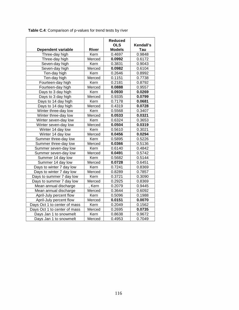
116

Table C.4: Comparison of p-values for trend tests by river

Dependent variable River

Reduced OLS

Models Kendall’s

Tau Three-day high Kern 0.4697 0.9848 Three-day high Merced 0.0992 0.6172 Seven-day high Kern 0.3831 0.9043 Seven-day high Merced 0.0982 0.6104 Ten-day high Kern 0.2646 0.8992 Ten-day high Merced 0.1151 0.7738

Fourteen-day high Kern 0.2181 0.8792 Fourteen-day high Merced 0.0888 0.9557 Days to 3 day high Kern 0.0930 0.0269 Days to 3 day high Merced 0.9335 0.0799 Days to 14 day high Kern 0.7178 0.0681 Days to 14 day high Merced 0.4319 0.0728 Winter three-day low Kern 0.5568 0.3407 Winter three-day low Merced 0.0533 0.0321 Winter seven-day low Kern 0.6324 0.3653 Winter seven-day low Merced 0.0504 0.0319

Winter 14 day low Kern 0.5610 0.3021 Winter 14 day low Merced 0.0456 0.0294

Summer three-day low Kern 0.5895 0.5226 Summer three-day low Merced 0.0366 0.5136 Summer seven-day low Kern 0.6140 0.4842 Summer seven-day low Merced 0.0491 0.5742

Summer 14 day low Kern 0.5682 0.5144 Summer 14 day low Merced 0.0728 0.6451

Days to winter 7 day low Kern 0.7241 0.8369 Days to winter 7 day low Merced 0.8289 0.7857

Days to summer 7 day low Kern 0.3721 0.3090 Days to summer 7 day low Merced 0.2925 0.8369

Mean annual discharge , Kern 0.2079 0.9445 Mean annual discharge Merced 0.3644 0.6092 April-July percent flow Kern 0.5096 0.1988 April-July percent flow Merced 0.0151 0.0070

Days Oct 1 to center of mass Kern 0.2049 0.1562 Days Oct 1 to center of mass Merced 0.2695 0.0735

Days Jan 1 to snowmelt Kern 0.8638 0.9672 Days Jan 1 to snowmelt Merced 0.4953 0.7049

117

Power Analysis The power of the parametric and nonparametric trend tests is examined with a Monte Carlo power simulation. The most recent estimates of status and estimates of residual error from the individual river analyses are used with the year-to-year variation estimates from the across-river analyses to simulate the populations of interest under known levels of trend. Note that variance components are taken from different trend analyses so that total variance may be overestimated. This approach is considered conservative but useful given the large impact of the year-to-year variation on the power to detect trend (Urquhart and Kincaid 1999). The simulated data are combined with the historic data for a complete data record for trend detection. Note that the trend is imposed only in the simulated data. The two-sided parametric and nonparametric trend tests are conducted and compared against a Type I error level of 0.10. A total of 1000 iterations are used to assess the power of each test as the proportion of times the test results in a correct rejection of the null hypothesis.

The results of the power analysis are provided in Figures C.15 through C.22. Note that the trend is assessed for the historic data as well as the simulated data. As expected, a trend of 4% annually is detected with higher power than an annual trend of 1%. Overall, the power to detect trends in flow metrics of 4% per year exceeds 80% within the 10 to 20 years of monitoring. Achieving 80% power to detect a 1% annual trend may take up to 40 years but most outcomes achieve 80% power within 20 to 30 years of monitoring. No outcome consistently performed with higher or lower power than the rest. Power for the Kendall tau-b test of trend is generally higher than that of the linear mixed model when the residual variation is relatively large for an outcome.

Power for the two tests is very similar with generally slightly higher power for the linear mixed model (LMM). This result is not surprising since the data are generated to meet the assumptions of least squares. One exception is found in the power plots for the number of days to the three-day high in the Merced River (Figure 17d). For this outcome, the power to detect a 1% annual trend is much higher for the first 10 years of the monitoring program then it drops before increasing monotonically again. This pattern is due to a significant negative trend detected in the pilot data by the Kendall tau-b test (Table 3) that is not detected by the linear mixed model (table 2). After additional years of data are observed, the power increases monotonically over time. Note that this is an artifact of the data; when the power to detect trend in this outcome is assessed without the historic data, the power increases monotonically for all monitoring periods. Because a significant negative trend was observed in the number of days to the three-day high in the Kern River and the percent flow between April and July in the Merced River, this simulation was conducted assuming a negative trend.

Because the power analysis for each river for a given outcome assumes the same estimate of year-to-year variation, the power for the river exhibiting less residual variation is generally higher. An exception occurs when the simulated trend is similar to that of the observed trend from the historic data. In these cases, the trend is consistent over the entire monitoring period so the power to detect this trend is higher than if no trend was observed for the first 93 to 96 years despite increased unexplained variation. This pattern is demonstrated by the winter three-, seven-, and fourteen-day lows for the Merced River (Figures C.18 and C.19).

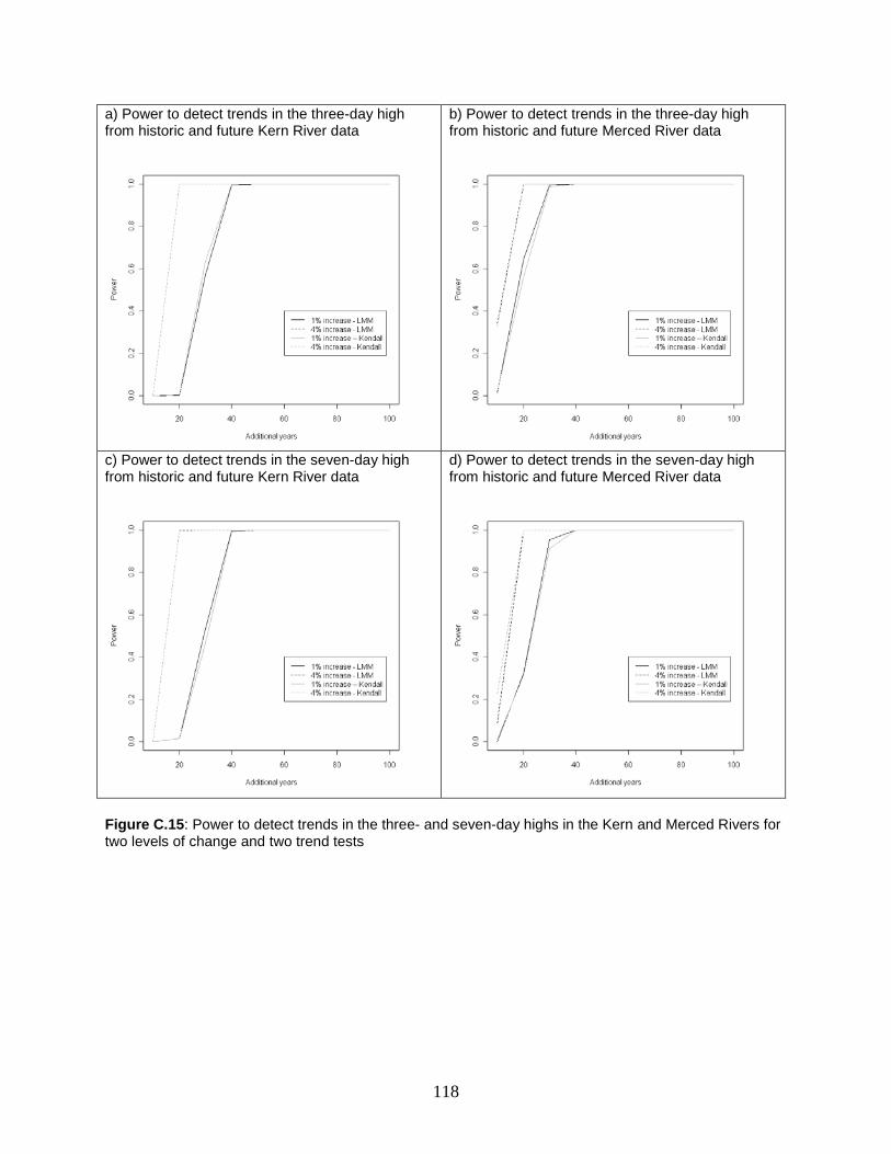
118

a) Power to detect trends in the three-day high from historic and future Kern River data

b) Power to detect trends in the three-day high from historic and future Merced River data

c) Power to detect trends in the seven-day high from historic and future Kern River data

d) Power to detect trends in the seven-day high from historic and future Merced River data

Figure C.15: Power to detect trends in the three- and seven-day highs in the Kern and Merced Rivers for two levels of change and two trend tests

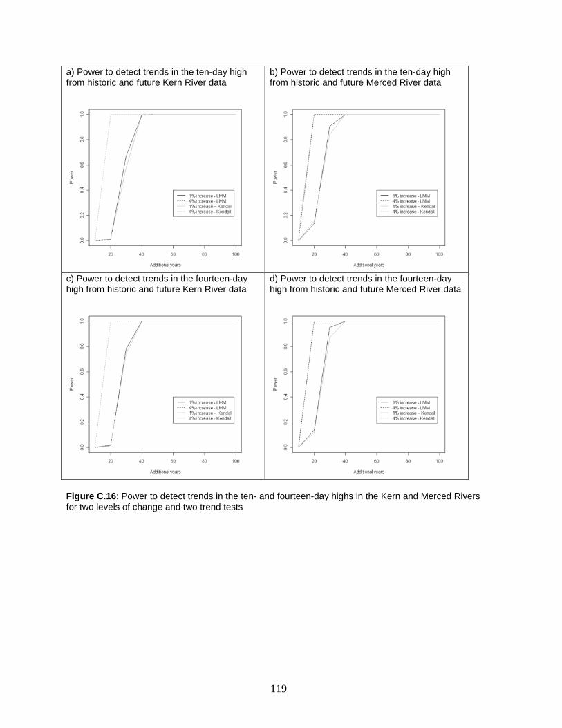
119

a) Power to detect trends in the ten-day high from historic and future Kern River data

b) Power to detect trends in the ten-day high from historic and future Merced River data

c) Power to detect trends in the fourteen-day high from historic and future Kern River data

d) Power to detect trends in the fourteen-day high from historic and future Merced River data

Figure C.16: Power to detect trends in the ten- and fourteen-day highs in the Kern and Merced Rivers for two levels of change and two trend tests

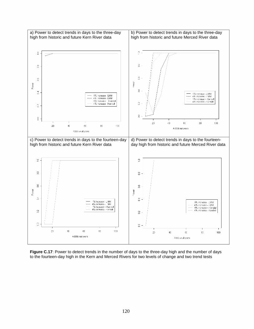
120

a) Power to detect trends in days to the three-day high from historic and future Kern River data

b) Power to detect trends in days to the three-day high from historic and future Merced River data

c) Power to detect trends in days to the fourteen-day high from historic and future Kern River data

d) Power to detect trends in days to the fourteen-day high from historic and future Merced River data

Figure C.17: Power to detect trends in the number of days to the three-day high and the number of days to the fourteen-day high in the Kern and Merced Rivers for two levels of change and two trend tests

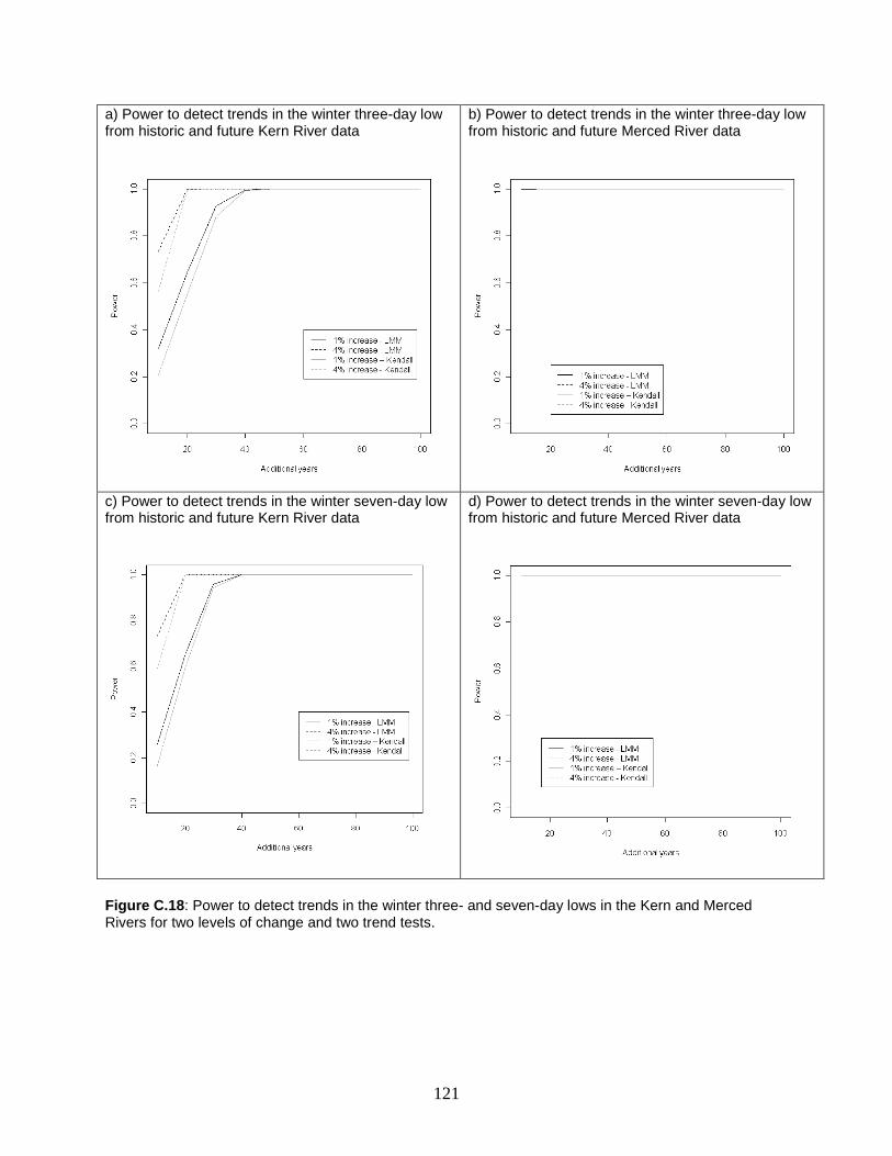
121

a) Power to detect trends in the winter three-day low from historic and future Kern River data

b) Power to detect trends in the winter three-day low from historic and future Merced River data

c) Power to detect trends in the winter seven-day low from historic and future Kern River data

d) Power to detect trends in the winter seven-day low from historic and future Merced River data

Figure C.18: Power to detect trends in the winter three- and seven-day lows in the Kern and Merced Rivers for two levels of change and two trend tests.

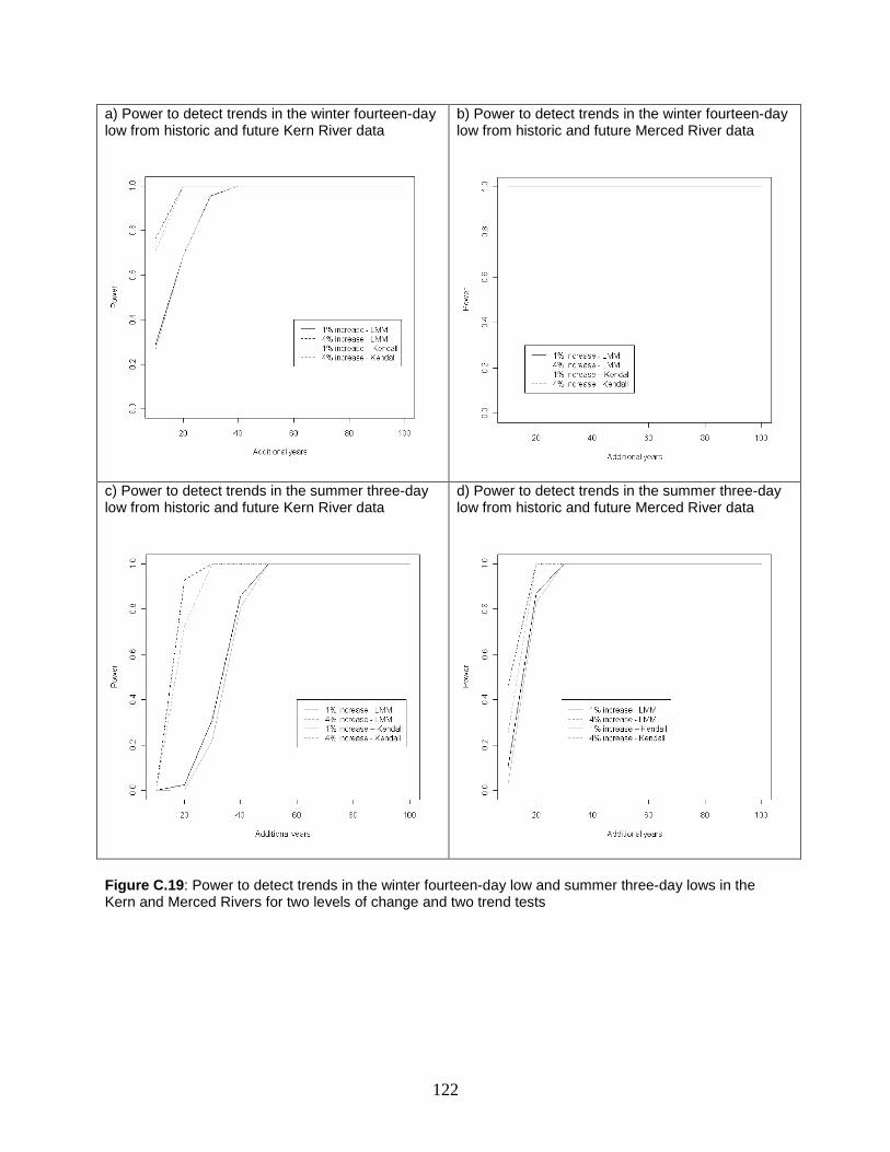
122

a) Power to detect trends in the winter fourteen-day low from historic and future Kern River data

b) Power to detect trends in the winter fourteen-day low from historic and future Merced River data

c) Power to detect trends in the summer three-day low from historic and future Kern River data

d) Power to detect trends in the summer three-day low from historic and future Merced River data

Figure C.19: Power to detect trends in the winter fourteen-day low and summer three-day lows in the Kern and Merced Rivers for two levels of change and two trend tests

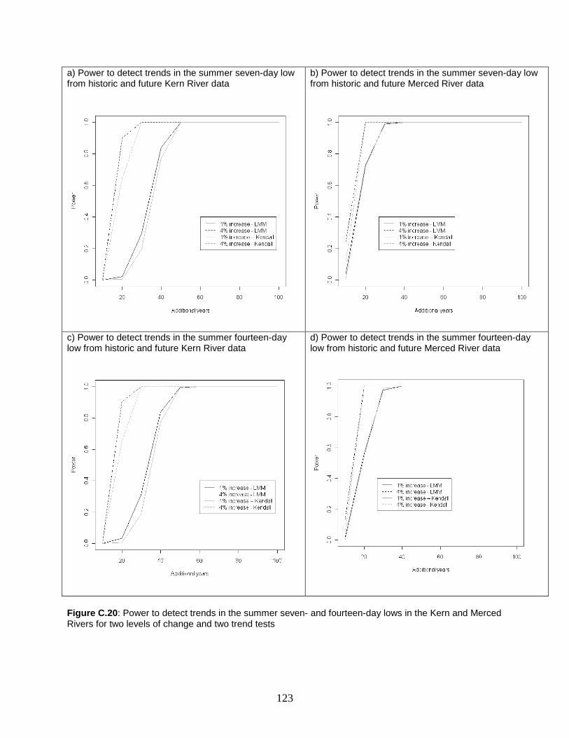
123

a) Power to detect trends in the summer seven-day low from historic and future Kern River data

b) Power to detect trends in the summer seven-day low from historic and future Merced River data

c) Power to detect trends in the summer fourteen-day low from historic and future Kern River data

d) Power to detect trends in the summer fourteen-day low from historic and future Merced River data

Figure C.20: Power to detect trends in the summer seven- and fourteen-day lows in the Kern and Merced Rivers for two levels of change and two trend tests

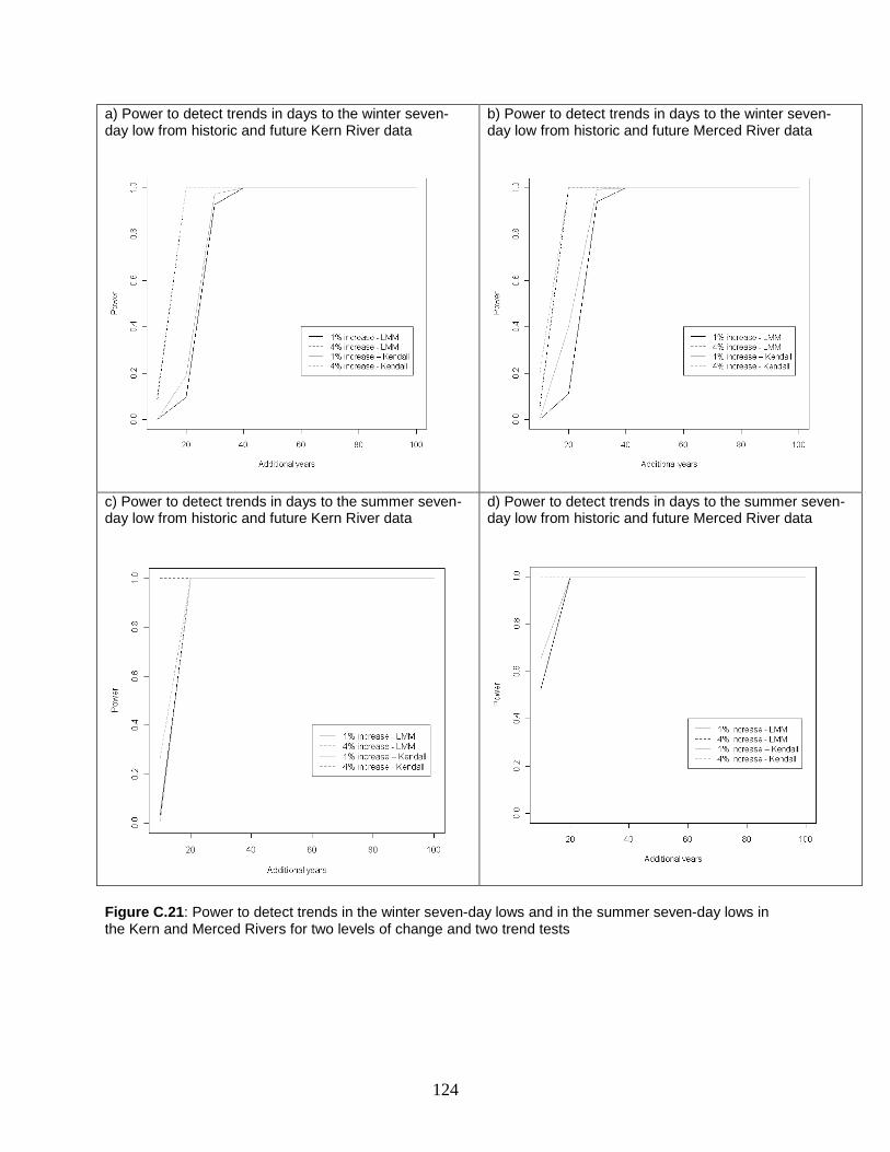
124

a) Power to detect trends in days to the winter seven-day low from historic and future Kern River data

b) Power to detect trends in days to the winter seven-day low from historic and future Merced River data

c) Power to detect trends in days to the summer seven-day low from historic and future Kern River data

d) Power to detect trends in days to the summer seven-day low from historic and future Merced River data

Figure C.21: Power to detect trends in the winter seven-day lows and in the summer seven-day lows in the Kern and Merced Rivers for two levels of change and two trend tests

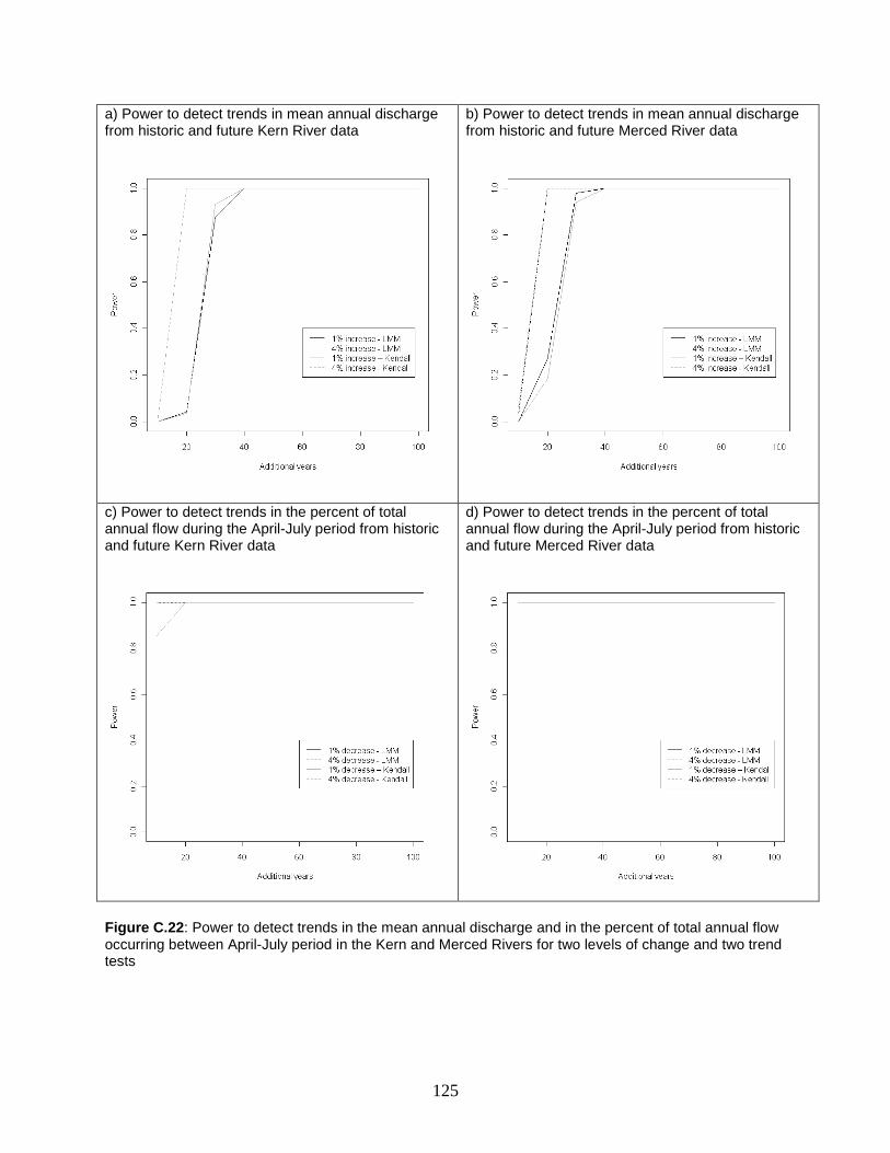
125

a) Power to detect trends in mean annual discharge from historic and future Kern River data

b) Power to detect trends in mean annual discharge from historic and future Merced River data

c) Power to detect trends in the percent of total annual flow during the April-July period from historic and future Kern River data

d) Power to detect trends in the percent of total annual flow during the April-July period from historic and future Merced River data

Figure C.22: Power to detect trends in the mean annual discharge and in the percent of total annual flow occurring between April-July period in the Kern and Merced Rivers for two levels of change and two trend tests

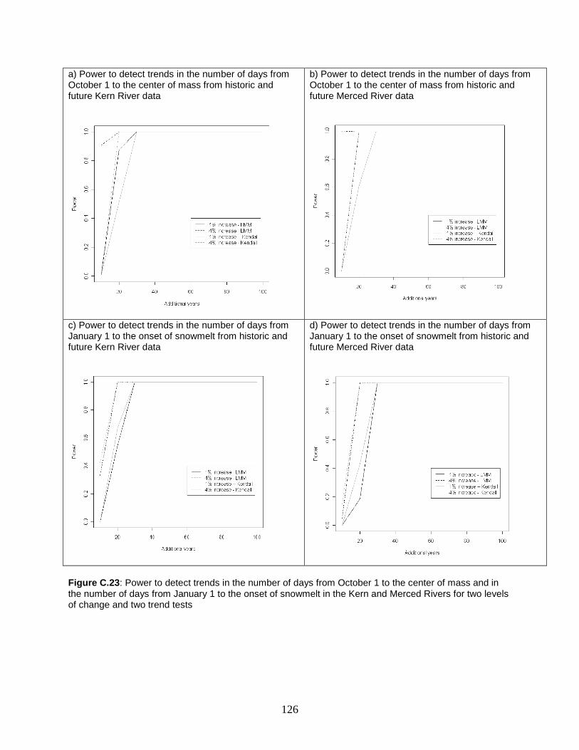
126

a) Power to detect trends in the number of days from October 1 to the center of mass from historic and future Kern River data

b) Power to detect trends in the number of days from October 1 to the center of mass from historic and future Merced River data

c) Power to detect trends in the number of days from January 1 to the onset of snowmelt from historic and future Kern River data

d) Power to detect trends in the number of days from January 1 to the onset of snowmelt from historic and future Merced River data

Figure C.23: Power to detect trends in the number of days from October 1 to the center of mass and in the number of days from January 1 to the onset of snowmelt in the Kern and Merced Rivers for two levels of change and two trend tests

127

Conclusions Overall, trends in the eighteen metrics describing flow conditions in the Merced and Kern Rivers were detectable with at least 80% power. If an increasing annual trend of 1% were observed during the next 100 years, the power to detect this trend would exceed 80% within 20 to 40 years for most outcomes. An annual trend of 4% would be detected with at least 80% power in no more than 20 years for all of the outcomes examined. Only the outcome measuring percent of total flow occurring between April and July exhibited high power for both rivers.

The trend test from a linear mixed model (Piepho and Ogutu 2002) demonstrated slightly higher power that the Kendall tau-b test (Higgins 2004) for most outcomes. However, examination of the test size (the Type I error rate demonstrated by the test) for both tests indicated that test size may be lower than nominal for the t-test from the linear mixed model when the sample of years is relatively small (less than 40 to 50 years). For these monitoring time frames, the Kendall tau-b exhibited test size closer to nominal levels and may provide more reliable inference for these shorter monitoring periods.

129

Appendix C. Literature Cited Andrews, E. D. 2012. Hydrology of the Sierra Nevada Network national parks: Status and

trends. Natural Resource Report NPS/SIEN/NRR—2012/500. National Park Service, Fort Collins, Colorado.

Elliott, P. E., Beck, D. A., and Prudic, D. E. 2006. Characterization of surface-water resources in the Great Basin National Park area and their susceptibility to ground-water withdrawals in adjacent valleys, White Pine County, Nevada: U.S. Geological Survey Scientific Investigations Report 2006-5099, 156 p. Available at URL: http://pubs.water.usgs.gov/sir2006-5099

Gilbert, R. O. 1987. Statistical Methods for Environmental Pollution Monitoring. Van Nosstrand Reinhold Company. New York.

.

Higgins J. J. 2004. Introduction to modern nonparametric statistics. Brooks/Cole-Thompson Learning. Pacific Grove, California.

Illinois Department of Energy and Natural Resources. 1994. The Changing Illinois Environment: Critical Trends. Summary Report and Volumes 1 - 7 Technical Report. Illinois Department of Energy and Natural Resources, Springfield, EL, ILENR/RE-EA-94A)5.

Kelly, V. J. and S. M. Jett. 2006. Ecologically-relevant quantification of streamflow regimes in western streams. EPA/620/R-06/056. U.S. Environmental Protection Agency, Washington, D.C.

Kenward, M.G. and J. H. Roger. 1997. Small sample inference for fixed effects from restricted maximum likelihood. Biometrics 53: 983–997.

Kuehl, R. O. 1994. Statistical Principles of Research Design and Analysis. Duxberry Press: Belmont, California. 686 pp.

Lettenmaier, D. P. 1976. Detection of trends in water quality data from records with dependent observations. Water Resources Research 12(5):1037-1046.

Page, E. B. 1963. Ordered hypothesis for multiple treatments: a significance test for linear ranks. Journal of the American Statistical Association. 58:216-230.

Piepho, H. P. and J. O. Ogutu. 2002. A simple mixed model for trend analysis in wildlife populations. Journal of Agricultural, Biological, and Environmental Statistics 7(3): 350-360.

Pinheiro, J. C. and D. M. Bates. 2004. Mixed-effects models in S and S-PLUS. Springer Science and Business Media, New York, NY

R Development Core Team. 2011. R: A language and environment for statistical computing. R Foundation for Statistical Computing, Vienna, Austria. ISBN 3-900051-07-0, URL http://www.R-project.org/.

http://www.r-project.org/�

130

Sargeant, D., D. Dugger, P. Anderson, and E. Newell. 2011. Surface Water Monitoring Program for Pesticides in Salmonid-Bearing Streams, 2009 Data Summary. Washington State Departments of Agriculture and Ecology. Publication No. 11-03-004.

Satterthwaite, F. E. 1946. An Approximate Distribution of Estimates of Variance Components. Biometrics Bulletin 2: 110–114.

Sen, P. K. 1968. Estimates of the regression coefficient based on Kendall’s Tau. Journal of the American Statistical Association. 63:1379-1389.

Spilke, J., H. P. Piepho, and X. Hu. 2005. Analysis of unbalanced data by mixed linear models using the MIXED procedure of the SAS system. Journal of Agronomy and Crop Science 191:47–54.

Urquhart, N. S., W. S. Overton and D. S. Birkes. 1993. Comparing sampling designs for ecological monitoring. V. Barnet and K. F. Turkman, eds. Statistics for the Environment, pp. 71 - 85. John Wiley and Sons, London.

Urquhart, N. S. and T. M. Kincaid. 1999. Designs for detecting trend from repeated surveys of ecological resources. Journal of Agricultural, Biological, and Environmental Statistics 4(4): 404-414.

USGS National Water Information System. 2011. http://nwis.waterdata.usgs.gov/nwis/sw

VanLeeuwen, D. M., L. W. Murray, and N. S. Urquhart. 1996. A mixed model with both fixed and random trend components across time. Journal of Agricultural, Biological, and Environmental Statistics 1(4): 435-453.

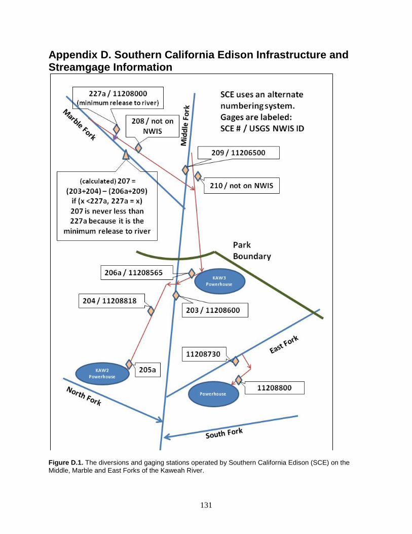
http://nwis.waterdata.usgs.gov/nwis/sw�

131

Appendix D. Southern California Edison Infrastructure and Streamgage Information

Figure D.1. The diversions and gaging stations operated by Southern California Edison (SCE) on the Middle, Marble and East Forks of the Kaweah River.

133

Appendix E. Administrative Record

Date Event

Dec 2005 First meeting of the water resources work group. Lakes and streams protocol general objectives discussed. Lakes and streams divided into two protocols. Lakes protocol set as first priority. Streams development delayed.

Feb 2008 Rivers/Streams protocol meeting with work group led by A. Heard to clarify objectives.

June 2010 SIEN term physical scientist hired to complete Rivers and streams protocol July 2010 Water work group meeting to prioritize protocol objectives. Water quantity and

timing prioritized over water quality if budget does not allow both. Sept/Oct 2010 SIEN protocol prioritization meeting and 3-year review with the SIEN steering

committee and BOD reveal rivers protocol is not prioritized but should proceed with development and assume ~$10,000 budget.

Oct 2010 Draft of SIEN surface water dynamics status and trends analysis complete (Andrews 2012). Andrews report results presented at YOSE hydroclimate meeting with SIEN cooperators. Discussion with cooperators about direction of rivers protocol.

Dec 2010 Water work group meeting to prioritize watersheds and stations for monitoring Feb 2011 Objectives and station selection rationale sent to water work group and

steering committee for approval. SIEN Physical Scientist and network manager meet with SEKI resource manager.

Mar 2011 SEKI resource manager submitted request for consideration of additional SEKI site prior to granting approval of site selection and objectives.

Protocol development summary finalized July 2011 LAH Starcevich (U Idaho) begins work on power analysis Sept 2011 Steering committee gives final approval to protocol objectives and sample

design. Oct 2011 First draft of protocol to SIEN program manager and data manager for review. Jan 2012 Final draft of rivers power analysis submitted to SIEN from U Idaho. Jan/Feb 2012 Protocol circulated to water work group, MOJN Physical Scientist, and SIEN

staff for internal peer review. Review comments received from all work group members.

Mar 2012 Final revisions. Formatting by UCBN technical editor. Apr 2012 Submission to PWR peer review process.

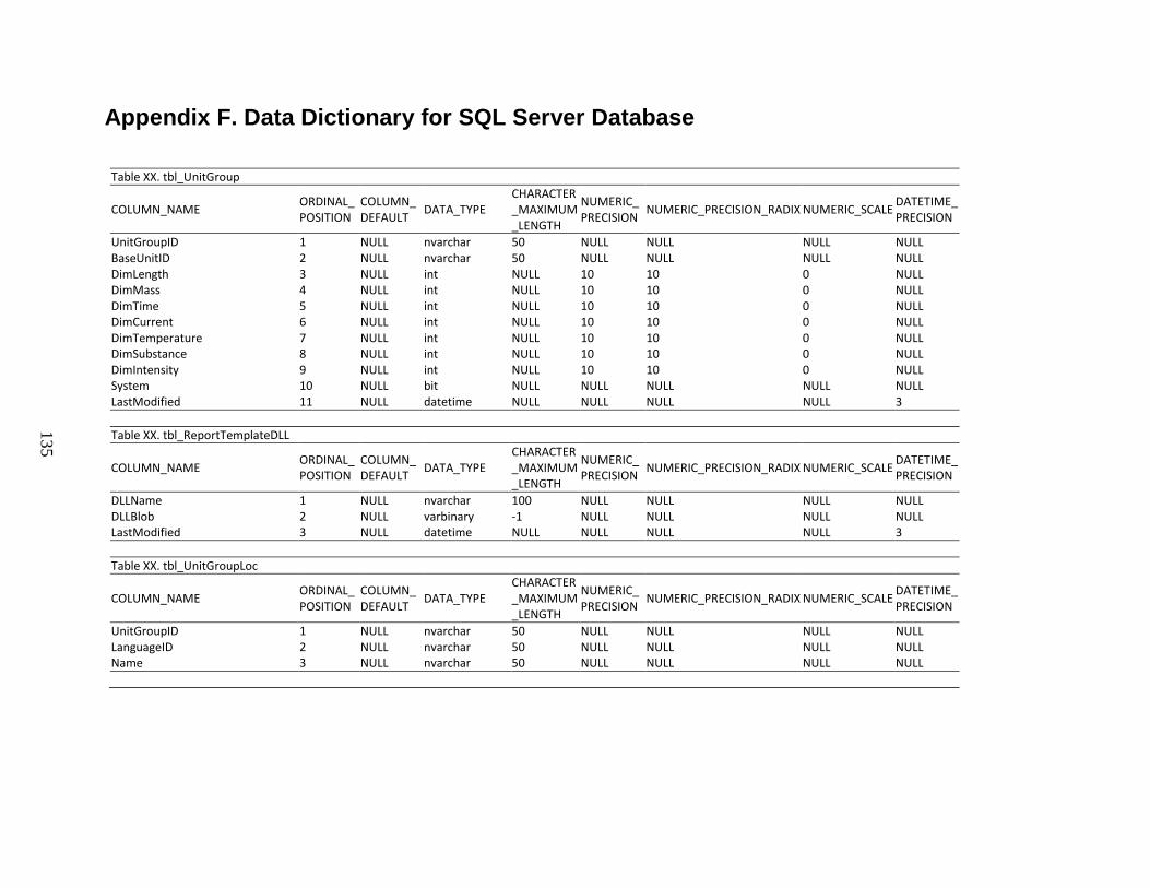
135

Appendix F. Data Dictionary for SQL Server Database

Table XX. tbl_UnitGroup

COLUMN_NAME ORDINAL_POSITION

COLUMN_DEFAULT DATA_TYPE

CHARACTER_MAXIMUM_LENGTH

NUMERIC_PRECISION NUMERIC_PRECISION_RADIX NUMERIC_SCALE DATETIME_

PRECISION

UnitGroupID 1 NULL nvarchar 50 NULL NULL NULL NULL BaseUnitID 2 NULL nvarchar 50 NULL NULL NULL NULL DimLength 3 NULL int NULL 10 10 0 NULL DimMass 4 NULL int NULL 10 10 0 NULL DimTime 5 NULL int NULL 10 10 0 NULL DimCurrent 6 NULL int NULL 10 10 0 NULL DimTemperature 7 NULL int NULL 10 10 0 NULL DimSubstance 8 NULL int NULL 10 10 0 NULL DimIntensity 9 NULL int NULL 10 10 0 NULL System 10 NULL bit NULL NULL NULL NULL NULL LastModified 11 NULL datetime NULL NULL NULL NULL 3 Table XX. tbl_ReportTemplateDLL





PRECISION

DLLName 1 NULL nvarchar 100 NULL NULL NULL NULL DLLBlob 2 NULL varbinary -1 NULL NULL NULL NULL LastModified 3 NULL datetime NULL NULL NULL NULL 3 Table XX. tbl_UnitGroupLoc





PRECISION

UnitGroupID 1 NULL nvarchar 50 NULL NULL NULL NULL LanguageID 2 NULL nvarchar 50 NULL NULL NULL NULL Name 3 NULL nvarchar 50 NULL NULL NULL NULL

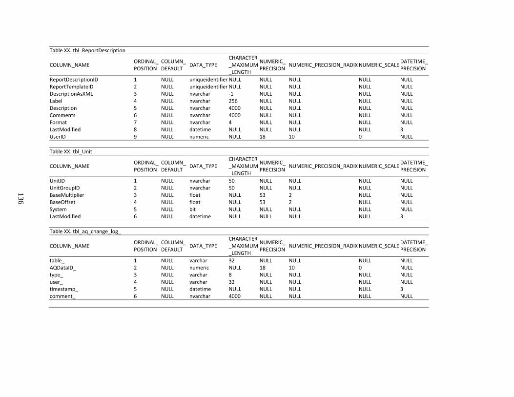
136

Table XX. tbl_ReportDescription





PRECISION

ReportDescriptionID 1 NULL uniqueidentifier NULL NULL NULL NULL NULL ReportTemplateID 2 NULL uniqueidentifier NULL NULL NULL NULL NULL DescriptionAsXML 3 NULL nvarchar -1 NULL NULL NULL NULL Label 4 NULL nvarchar 256 NULL NULL NULL NULL Description 5 NULL nvarchar 4000 NULL NULL NULL NULL Comments 6 NULL nvarchar 4000 NULL NULL NULL NULL Format 7 NULL nvarchar 4 NULL NULL NULL NULL LastModified 8 NULL datetime NULL NULL NULL NULL 3 UserID 9 NULL numeric NULL 18 10 0 NULL Table XX. tbl_Unit





PRECISION

UnitID 1 NULL nvarchar 50 NULL NULL NULL NULL UnitGroupID 2 NULL nvarchar 50 NULL NULL NULL NULL BaseMultiplier 3 NULL float NULL 53 2 NULL NULL BaseOffset 4 NULL float NULL 53 2 NULL NULL System 5 NULL bit NULL NULL NULL NULL NULL LastModified 6 NULL datetime NULL NULL NULL NULL 3 Table XX. tbl_aq_change_log_





PRECISION

table_ 1 NULL varchar 32 NULL NULL NULL NULL AQDataID_ 2 NULL numeric NULL 18 10 0 NULL type_ 3 NULL varchar 8 NULL NULL NULL NULL user_ 4 NULL varchar 32 NULL NULL NULL NULL timestamp_ 5 NULL datetime NULL NULL NULL NULL 3 comment_ 6 NULL nvarchar 4000 NULL NULL NULL NULL

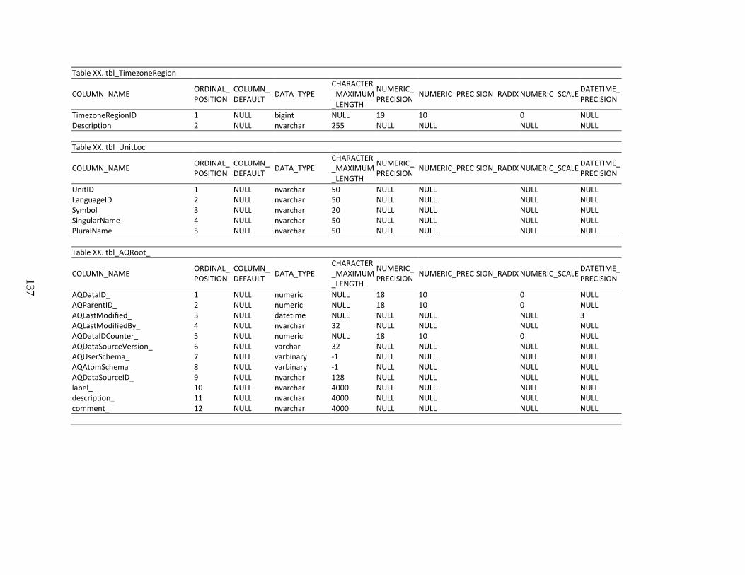
137

Table XX. tbl_TimezoneRegion





PRECISION

TimezoneRegionID 1 NULL bigint NULL 19 10 0 NULL Description 2 NULL nvarchar 255 NULL NULL NULL NULL Table XX. tbl_UnitLoc





PRECISION

UnitID 1 NULL nvarchar 50 NULL NULL NULL NULL LanguageID 2 NULL nvarchar 50 NULL NULL NULL NULL Symbol 3 NULL nvarchar 20 NULL NULL NULL NULL SingularName 4 NULL nvarchar 50 NULL NULL NULL NULL PluralName 5 NULL nvarchar 50 NULL NULL NULL NULL Table XX. tbl_AQRoot_





PRECISION

AQDataID_ 1 NULL numeric NULL 18 10 0 NULL AQParentID_ 2 NULL numeric NULL 18 10 0 NULL AQLastModified_ 3 NULL datetime NULL NULL NULL NULL 3 AQLastModifiedBy_ 4 NULL nvarchar 32 NULL NULL NULL NULL AQDataIDCounter_ 5 NULL numeric NULL 18 10 0 NULL AQDataSourceVersion_ 6 NULL varchar 32 NULL NULL NULL NULL AQUserSchema_ 7 NULL varbinary -1 NULL NULL NULL NULL AQAtomSchema_ 8 NULL varbinary -1 NULL NULL NULL NULL AQDataSourceID_ 9 NULL nvarchar 128 NULL NULL NULL NULL label_ 10 NULL nvarchar 4000 NULL NULL NULL NULL description_ 11 NULL nvarchar 4000 NULL NULL NULL NULL comment_ 12 NULL nvarchar 4000 NULL NULL NULL NULL

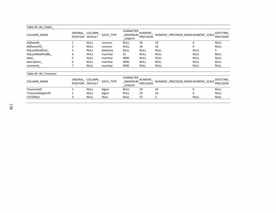
138

Table XX. tbl_Folder_





PRECISION

AQDataID_ 1 NULL numeric NULL 18 10 0 NULL AQParentID_ 2 NULL numeric NULL 18 10 0 NULL AQLastModified_ 3 NULL datetime NULL NULL NULL NULL 3 AQLastModifiedBy_ 4 NULL nvarchar 32 NULL NULL NULL NULL label_ 5 NULL nvarchar 4000 NULL NULL NULL NULL description_ 6 NULL nvarchar 4000 NULL NULL NULL NULL comment_ 7 NULL nvarchar 4000 NULL NULL NULL NULL Table XX. tbl_Timezone





PRECISION

TimezoneID 1 NULL bigint NULL 19 10 0 NULL TimezoneRegionID 2 NULL bigint NULL 19 10 0 NULL UTCOffset 3 NULL float NULL 53 2 NULL NULL

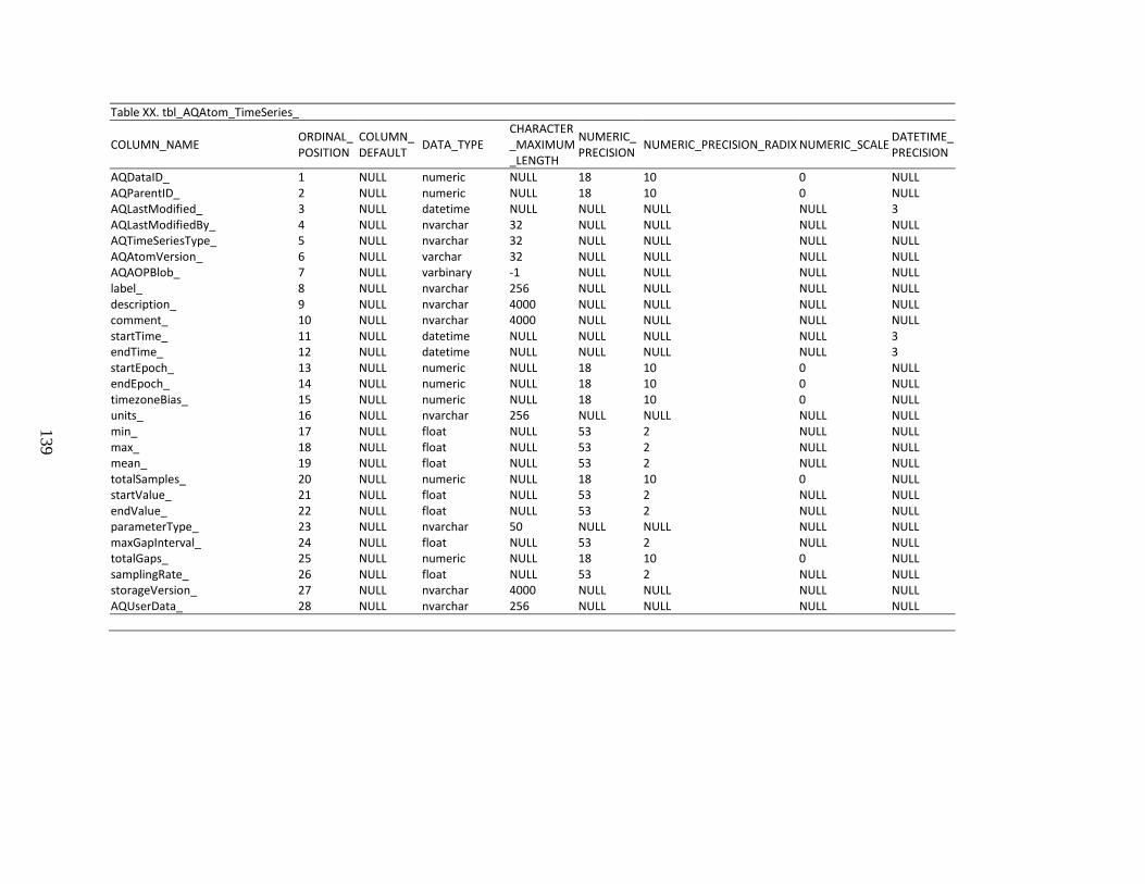
139

Table XX. tbl_AQAtom_TimeSeries_





PRECISION

AQDataID_ 1 NULL numeric NULL 18 10 0 NULL AQParentID_ 2 NULL numeric NULL 18 10 0 NULL AQLastModified_ 3 NULL datetime NULL NULL NULL NULL 3 AQLastModifiedBy_ 4 NULL nvarchar 32 NULL NULL NULL NULL AQTimeSeriesType_ 5 NULL nvarchar 32 NULL NULL NULL NULL AQAtomVersion_ 6 NULL varchar 32 NULL NULL NULL NULL AQAOPBlob_ 7 NULL varbinary -1 NULL NULL NULL NULL label_ 8 NULL nvarchar 256 NULL NULL NULL NULL description_ 9 NULL nvarchar 4000 NULL NULL NULL NULL comment_ 10 NULL nvarchar 4000 NULL NULL NULL NULL startTime_ 11 NULL datetime NULL NULL NULL NULL 3 endTime_ 12 NULL datetime NULL NULL NULL NULL 3 startEpoch_ 13 NULL numeric NULL 18 10 0 NULL endEpoch_ 14 NULL numeric NULL 18 10 0 NULL timezoneBias_ 15 NULL numeric NULL 18 10 0 NULL units_ 16 NULL nvarchar 256 NULL NULL NULL NULL min_ 17 NULL float NULL 53 2 NULL NULL max_ 18 NULL float NULL 53 2 NULL NULL mean_ 19 NULL float NULL 53 2 NULL NULL totalSamples_ 20 NULL numeric NULL 18 10 0 NULL startValue_ 21 NULL float NULL 53 2 NULL NULL endValue_ 22 NULL float NULL 53 2 NULL NULL parameterType_ 23 NULL nvarchar 50 NULL NULL NULL NULL maxGapInterval_ 24 NULL float NULL 53 2 NULL NULL totalGaps_ 25 NULL numeric NULL 18 10 0 NULL samplingRate_ 26 NULL float NULL 53 2 NULL NULL storageVersion_ 27 NULL nvarchar 4000 NULL NULL NULL NULL AQUserData_ 28 NULL nvarchar 256 NULL NULL NULL NULL

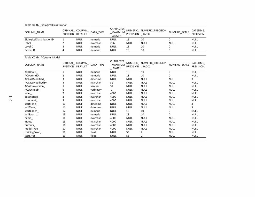
140

Table XX. tbl_BiologicalClassification




NUMERIC_PRECISION

NUMERIC_PRECISION_RADIX NUMERIC_SCALE DATETIME_

PRECISION

BiologicalClassificationID 1 NULL numeric NULL 18 10 0 NULL Label 2 NULL nvarchar 256 NULL NULL NULL NULL LevelID 3 NULL numeric NULL 18 10 0 NULL ParentID 4 NULL numeric NULL 18 10 0 NULL Table XX. tbl_AQAtom_Model_




NUMERIC_PRECISION


PRECISION

AQDataID_ 1 NULL numeric NULL 18 10 0 NULL AQParentID_ 2 NULL numeric NULL 18 10 0 NULL AQLastModified_ 3 NULL datetime NULL NULL NULL NULL 3 AQLastModifiedBy_ 4 NULL nvarchar 32 NULL NULL NULL NULL AQAtomVersion_ 5 NULL varchar 32 NULL NULL NULL NULL AQAOPBlob_ 6 NULL varbinary -1 NULL NULL NULL NULL label_ 7 NULL nvarchar 4000 NULL NULL NULL NULL description_ 8 NULL nvarchar 4000 NULL NULL NULL NULL comment_ 9 NULL nvarchar 4000 NULL NULL NULL NULL startTime_ 10 NULL datetime NULL NULL NULL NULL 3 endTime_ 11 NULL datetime NULL NULL NULL NULL 3 startEpoch_ 12 NULL numeric NULL 18 10 0 NULL endEpoch_ 13 NULL numeric NULL 18 10 0 NULL name_ 14 NULL nvarchar 4000 NULL NULL NULL NULL inputs_ 15 NULL nvarchar 4000 NULL NULL NULL NULL outputs_ 16 NULL nvarchar 4000 NULL NULL NULL NULL modelType_ 17 NULL nvarchar 4000 NULL NULL NULL NULL trainingError_ 18 NULL float NULL 53 2 NULL NULL testError_ 19 NULL float NULL 53 2 NULL NULL

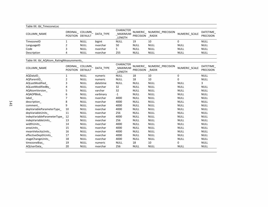
141

Table XX. tbl_TimezoneLoc




NUMERIC_PRECISION


PRECISION

TimezoneID 1 NULL bigint NULL 19 10 0 NULL LanguageID 2 NULL nvarchar 50 NULL NULL NULL NULL Code 3 NULL nvarchar 5 NULL NULL NULL NULL Description 4 NULL nvarchar 255 NULL NULL NULL NULL Table XX. tbl_AQAtom_RatingMeasurements_




NUMERIC_PRECISION


PRECISION

AQDataID_ 1 NULL numeric NULL 18 10 0 NULL AQParentID_ 2 NULL numeric NULL 18 10 0 NULL AQLastModified_ 3 NULL datetime NULL NULL NULL NULL 3 AQLastModifiedBy_ 4 NULL nvarchar 32 NULL NULL NULL NULL AQAtomVersion_ 5 NULL varchar 32 NULL NULL NULL NULL AQAOPBlob_ 6 NULL varbinary -1 NULL NULL NULL NULL label_ 7 NULL nvarchar 4000 NULL NULL NULL NULL description_ 8 NULL nvarchar 4000 NULL NULL NULL NULL comment_ 9 NULL nvarchar 4000 NULL NULL NULL NULL depVariableParameterType_ 10 NULL nvarchar 4000 NULL NULL NULL NULL depVariableUnits_ 11 NULL nvarchar 256 NULL NULL NULL NULL indepVariableParameterType_ 12 NULL nvarchar 4000 NULL NULL NULL NULL indepVariableUnits_ 13 NULL nvarchar 256 NULL NULL NULL NULL widthUnits_ 14 NULL nvarchar 4000 NULL NULL NULL NULL areaUnits_ 15 NULL nvarchar 4000 NULL NULL NULL NULL meanVelocityUnits_ 16 NULL nvarchar 4000 NULL NULL NULL NULL effectiveDepthUnits_ 17 NULL nvarchar 4000 NULL NULL NULL NULL stageChangeUnits_ 18 NULL nvarchar 4000 NULL NULL NULL NULL timezoneBias_ 19 NULL numeric NULL 18 10 0 NULL AQUserData_ 20 NULL nvarchar 256 NULL NULL NULL NULL

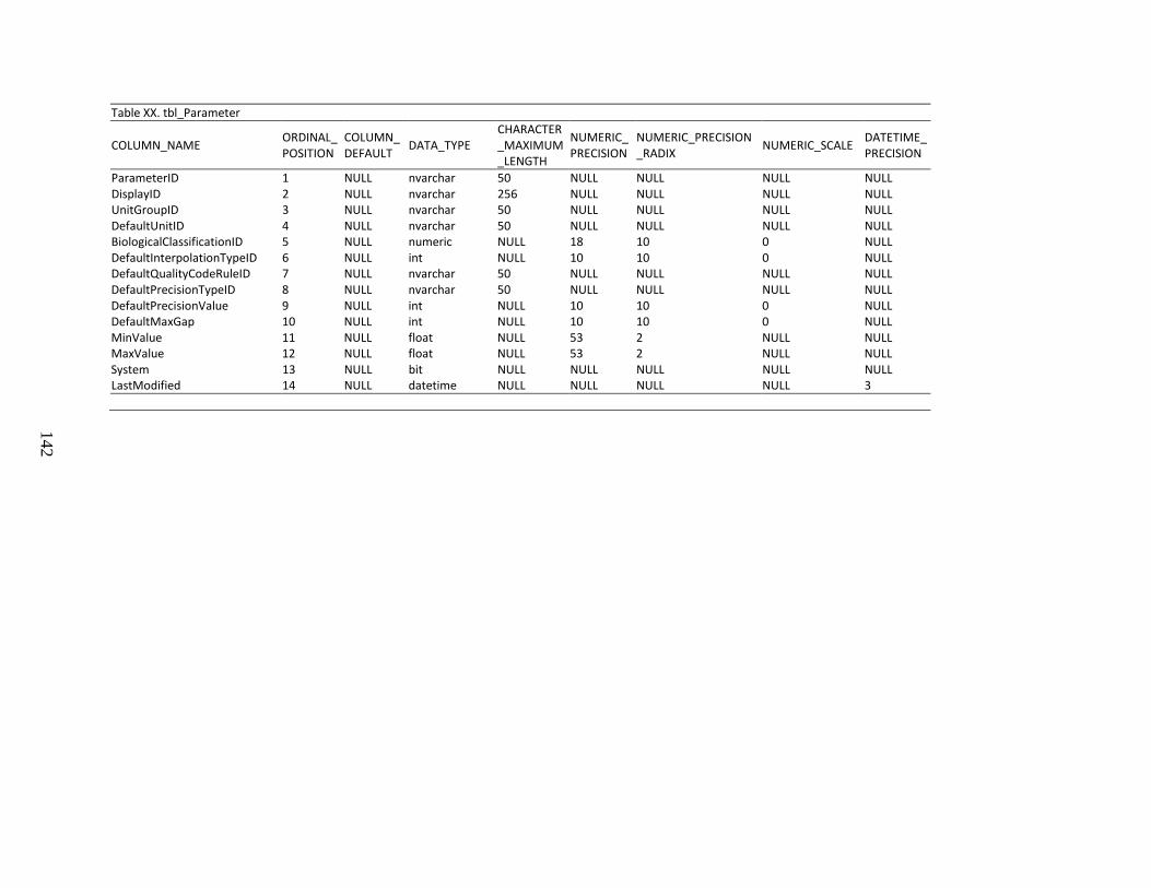
142

Table XX. tbl_Parameter




NUMERIC_PRECISION


PRECISION

ParameterID 1 NULL nvarchar 50 NULL NULL NULL NULL DisplayID 2 NULL nvarchar 256 NULL NULL NULL NULL UnitGroupID 3 NULL nvarchar 50 NULL NULL NULL NULL DefaultUnitID 4 NULL nvarchar 50 NULL NULL NULL NULL BiologicalClassificationID 5 NULL numeric NULL 18 10 0 NULL DefaultInterpolationTypeID 6 NULL int NULL 10 10 0 NULL DefaultQualityCodeRuleID 7 NULL nvarchar 50 NULL NULL NULL NULL DefaultPrecisionTypeID 8 NULL nvarchar 50 NULL NULL NULL NULL DefaultPrecisionValue 9 NULL int NULL 10 10 0 NULL DefaultMaxGap 10 NULL int NULL 10 10 0 NULL MinValue 11 NULL float NULL 53 2 NULL NULL MaxValue 12 NULL float NULL 53 2 NULL NULL System 13 NULL bit NULL NULL NULL NULL NULL LastModified 14 NULL datetime NULL NULL NULL NULL 3

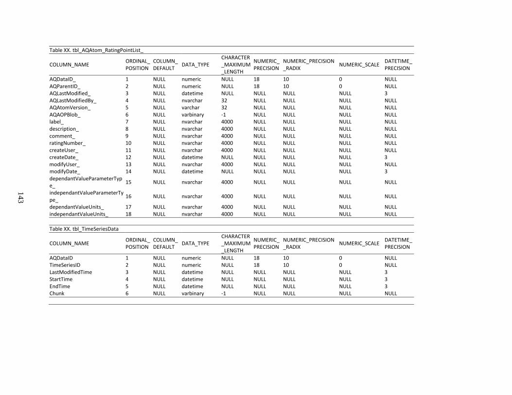
143

Table XX. tbl_AQAtom_RatingPointList_




NUMERIC_PRECISION


PRECISION

AQDataID_ 1 NULL numeric NULL 18 10 0 NULL AQParentID_ 2 NULL numeric NULL 18 10 0 NULL AQLastModified_ 3 NULL datetime NULL NULL NULL NULL 3 AQLastModifiedBy_ 4 NULL nvarchar 32 NULL NULL NULL NULL AQAtomVersion_ 5 NULL varchar 32 NULL NULL NULL NULL AQAOPBlob_ 6 NULL varbinary -1 NULL NULL NULL NULL label_ 7 NULL nvarchar 4000 NULL NULL NULL NULL description_ 8 NULL nvarchar 4000 NULL NULL NULL NULL comment_ 9 NULL nvarchar 4000 NULL NULL NULL NULL ratingNumber_ 10 NULL nvarchar 4000 NULL NULL NULL NULL createUser_ 11 NULL nvarchar 4000 NULL NULL NULL NULL createDate_ 12 NULL datetime NULL NULL NULL NULL 3 modifyUser_ 13 NULL nvarchar 4000 NULL NULL NULL NULL modifyDate_ 14 NULL datetime NULL NULL NULL NULL 3 dependantValueParameterType_ 15 NULL nvarchar 4000 NULL NULL NULL NULL

independantValueParameterType_ 16 NULL nvarchar 4000 NULL NULL NULL NULL

dependantValueUnits_ 17 NULL nvarchar 4000 NULL NULL NULL NULL independantValueUnits_ 18 NULL nvarchar 4000 NULL NULL NULL NULL Table XX. tbl_TimeSeriesData




NUMERIC_PRECISION


PRECISION

AQDataID 1 NULL numeric NULL 18 10 0 NULL TimeSeriesID 2 NULL numeric NULL 18 10 0 NULL LastModifiedTime 3 NULL datetime NULL NULL NULL NULL 3 StartTime 4 NULL datetime NULL NULL NULL NULL 3 EndTime 5 NULL datetime NULL NULL NULL NULL 3 Chunk 6 NULL varbinary -1 NULL NULL NULL NULL

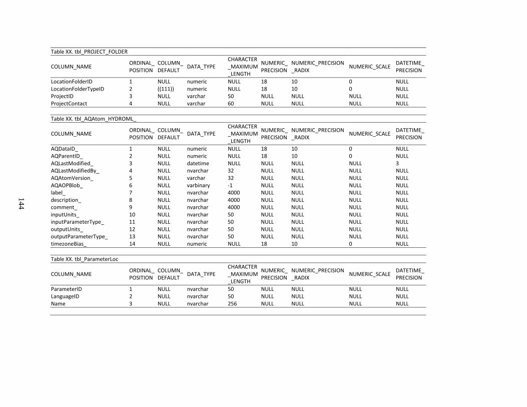
144

Table XX. tbl_PROJECT_FOLDER




NUMERIC_PRECISION


PRECISION

LocationFolderID 1 NULL numeric NULL 18 10 0 NULL LocationFolderTypeID 2 ((111)) numeric NULL 18 10 0 NULL ProjectID 3 NULL varchar 50 NULL NULL NULL NULL ProjectContact 4 NULL varchar 60 NULL NULL NULL NULL Table XX. tbl_AQAtom_HYDROML_




NUMERIC_PRECISION


PRECISION

AQDataID_ 1 NULL numeric NULL 18 10 0 NULL AQParentID_ 2 NULL numeric NULL 18 10 0 NULL AQLastModified_ 3 NULL datetime NULL NULL NULL NULL 3 AQLastModifiedBy_ 4 NULL nvarchar 32 NULL NULL NULL NULL AQAtomVersion_ 5 NULL varchar 32 NULL NULL NULL NULL AQAOPBlob_ 6 NULL varbinary -1 NULL NULL NULL NULL label_ 7 NULL nvarchar 4000 NULL NULL NULL NULL description_ 8 NULL nvarchar 4000 NULL NULL NULL NULL comment_ 9 NULL nvarchar 4000 NULL NULL NULL NULL inputUnits_ 10 NULL nvarchar 50 NULL NULL NULL NULL inputParameterType_ 11 NULL nvarchar 50 NULL NULL NULL NULL outputUnits_ 12 NULL nvarchar 50 NULL NULL NULL NULL outputParameterType_ 13 NULL nvarchar 50 NULL NULL NULL NULL timezoneBias_ 14 NULL numeric NULL 18 10 0 NULL Table XX. tbl_ParameterLoc




NUMERIC_PRECISION


PRECISION

ParameterID 1 NULL nvarchar 50 NULL NULL NULL NULL LanguageID 2 NULL nvarchar 50 NULL NULL NULL NULL Name 3 NULL nvarchar 256 NULL NULL NULL NULL

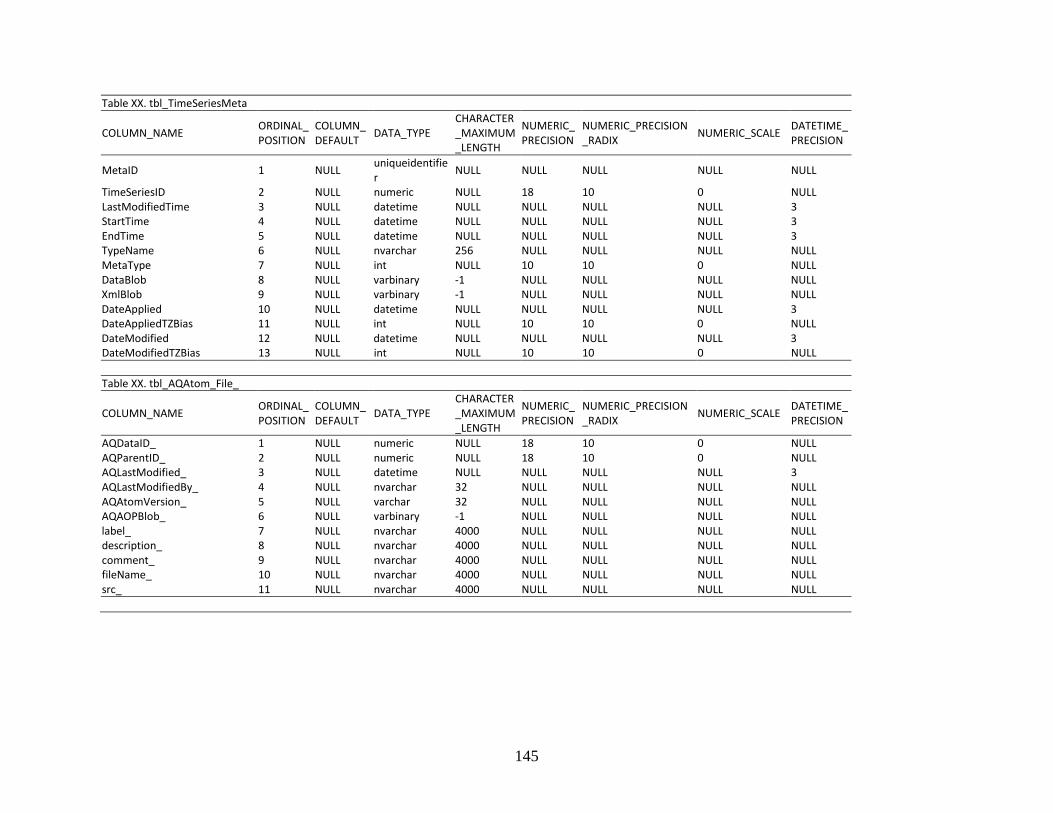
145

Table XX. tbl_TimeSeriesMeta




NUMERIC_PRECISION


PRECISION

MetaID 1 NULL uniqueidentifier NULL NULL NULL NULL NULL

TimeSeriesID 2 NULL numeric NULL 18 10 0 NULL LastModifiedTime 3 NULL datetime NULL NULL NULL NULL 3 StartTime 4 NULL datetime NULL NULL NULL NULL 3 EndTime 5 NULL datetime NULL NULL NULL NULL 3 TypeName 6 NULL nvarchar 256 NULL NULL NULL NULL MetaType 7 NULL int NULL 10 10 0 NULL DataBlob 8 NULL varbinary -1 NULL NULL NULL NULL XmlBlob 9 NULL varbinary -1 NULL NULL NULL NULL DateApplied 10 NULL datetime NULL NULL NULL NULL 3 DateAppliedTZBias 11 NULL int NULL 10 10 0 NULL DateModified 12 NULL datetime NULL NULL NULL NULL 3 DateModifiedTZBias 13 NULL int NULL 10 10 0 NULL Table XX. tbl_AQAtom_File_




NUMERIC_PRECISION


PRECISION

AQDataID_ 1 NULL numeric NULL 18 10 0 NULL AQParentID_ 2 NULL numeric NULL 18 10 0 NULL AQLastModified_ 3 NULL datetime NULL NULL NULL NULL 3 AQLastModifiedBy_ 4 NULL nvarchar 32 NULL NULL NULL NULL AQAtomVersion_ 5 NULL varchar 32 NULL NULL NULL NULL AQAOPBlob_ 6 NULL varbinary -1 NULL NULL NULL NULL label_ 7 NULL nvarchar 4000 NULL NULL NULL NULL description_ 8 NULL nvarchar 4000 NULL NULL NULL NULL comment_ 9 NULL nvarchar 4000 NULL NULL NULL NULL fileName_ 10 NULL nvarchar 4000 NULL NULL NULL NULL src_ 11 NULL nvarchar 4000 NULL NULL NULL NULL

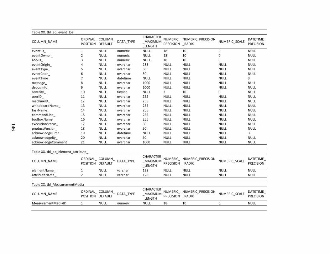
146

Table XX. tbl_aq_event_log_




NUMERIC_PRECISION


PRECISION

eventID_ 1 NULL numeric NULL 18 10 0 NULL eventOwner_ 2 NULL numeric NULL 18 10 0 NULL aopID_ 3 NULL numeric NULL 18 10 0 NULL eventOrigin_ 4 NULL nvarchar 255 NULL NULL NULL NULL eventType_ 5 NULL nvarchar 50 NULL NULL NULL NULL eventCode_ 6 NULL nvarchar 50 NULL NULL NULL NULL eventTime_ 7 NULL datetime NULL NULL NULL NULL 3 message_ 8 NULL nvarchar 1000 NULL NULL NULL NULL debugInfo_ 9 NULL nvarchar 1000 NULL NULL NULL NULL severity_ 10 NULL tinyint NULL 3 10 0 NULL userID_ 11 NULL nvarchar 255 NULL NULL NULL NULL machineID_ 12 NULL nvarchar 255 NULL NULL NULL NULL whiteboardName_ 13 NULL nvarchar 255 NULL NULL NULL NULL taskName_ 14 NULL nvarchar 255 NULL NULL NULL NULL commandLine_ 15 NULL nvarchar 255 NULL NULL NULL NULL toolboxName_ 16 NULL nvarchar 255 NULL NULL NULL NULL executionStatus_ 17 NULL nvarchar 50 NULL NULL NULL NULL productVersion_ 18 NULL nvarchar 50 NULL NULL NULL NULL acknowledgeTime_ 19 NULL datetime NULL NULL NULL NULL 3 acknowledgeBy_ 20 NULL nvarchar 50 NULL NULL NULL NULL acknowledgeComment_ 21 NULL nvarchar 1000 NULL NULL NULL NULL Table XX. tbl_aq_element_attribute_




NUMERIC_PRECISION


PRECISION

elementName_ 1 NULL varchar 128 NULL NULL NULL NULL attributeName_ 2 NULL varchar 128 NULL NULL NULL NULL Table XX. tbl_MeasurementMedia




NUMERIC_PRECISION


PRECISION

MeasurementMediaID 1 NULL numeric NULL 18 10 0 NULL

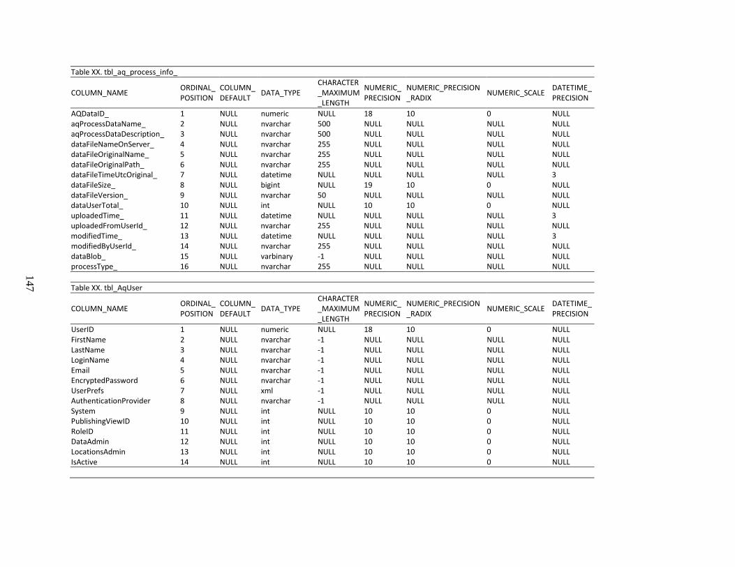
147

Table XX. tbl_aq_process_info_




NUMERIC_PRECISION


PRECISION

AQDataID_ 1 NULL numeric NULL 18 10 0 NULL aqProcessDataName_ 2 NULL nvarchar 500 NULL NULL NULL NULL aqProcessDataDescription_ 3 NULL nvarchar 500 NULL NULL NULL NULL dataFileNameOnServer_ 4 NULL nvarchar 255 NULL NULL NULL NULL dataFileOriginalName_ 5 NULL nvarchar 255 NULL NULL NULL NULL dataFileOriginalPath_ 6 NULL nvarchar 255 NULL NULL NULL NULL dataFileTimeUtcOriginal_ 7 NULL datetime NULL NULL NULL NULL 3 dataFileSize_ 8 NULL bigint NULL 19 10 0 NULL dataFileVersion_ 9 NULL nvarchar 50 NULL NULL NULL NULL dataUserTotal_ 10 NULL int NULL 10 10 0 NULL uploadedTime_ 11 NULL datetime NULL NULL NULL NULL 3 uploadedFromUserId_ 12 NULL nvarchar 255 NULL NULL NULL NULL modifiedTime_ 13 NULL datetime NULL NULL NULL NULL 3 modifiedByUserId_ 14 NULL nvarchar 255 NULL NULL NULL NULL dataBlob_ 15 NULL varbinary -1 NULL NULL NULL NULL processType_ 16 NULL nvarchar 255 NULL NULL NULL NULL Table XX. tbl_AqUser




NUMERIC_PRECISION


PRECISION

UserID 1 NULL numeric NULL 18 10 0 NULL FirstName 2 NULL nvarchar -1 NULL NULL NULL NULL LastName 3 NULL nvarchar -1 NULL NULL NULL NULL LoginName 4 NULL nvarchar -1 NULL NULL NULL NULL Email 5 NULL nvarchar -1 NULL NULL NULL NULL EncryptedPassword 6 NULL nvarchar -1 NULL NULL NULL NULL UserPrefs 7 NULL xml -1 NULL NULL NULL NULL AuthenticationProvider 8 NULL nvarchar -1 NULL NULL NULL NULL System 9 NULL int NULL 10 10 0 NULL PublishingViewID 10 NULL int NULL 10 10 0 NULL RoleID 11 NULL int NULL 10 10 0 NULL DataAdmin 12 NULL int NULL 10 10 0 NULL LocationsAdmin 13 NULL int NULL 10 10 0 NULL IsActive 14 NULL int NULL 10 10 0 NULL

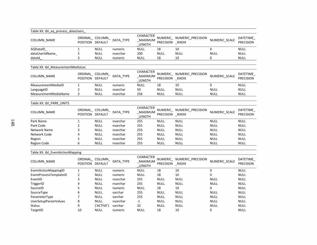
148

Table XX. tbl_aq_process_dataUsers_




NUMERIC_PRECISION


PRECISION

AQDataID_ 1 NULL numeric NULL 18 10 0 NULL dataUserIdName_ 2 NULL nvarchar 200 NULL NULL NULL NULL dataId_ 3 NULL numeric NULL 18 10 0 NULL Table XX. tbl_MeasurementMediaLoc




NUMERIC_PRECISION


PRECISION

MeasurementMediaID 1 NULL numeric NULL 18 10 0 NULL LanguageID 2 NULL nvarchar 50 NULL NULL NULL NULL MeasurementMediaName 3 NULL nvarchar 256 NULL NULL NULL NULL Table XX. tbl_PARK_UNITS




NUMERIC_PRECISION


PRECISION

Park Name 1 NULL nvarchar 255 NULL NULL NULL NULL Park Code 2 NULL nvarchar 255 NULL NULL NULL NULL Network Name 3 NULL nvarchar 255 NULL NULL NULL NULL Network Code 4 NULL nvarchar 255 NULL NULL NULL NULL Region 5 NULL nvarchar 255 NULL NULL NULL NULL Region Code 6 NULL nvarchar 255 NULL NULL NULL NULL Table XX. tbl_EventActionMapping




NUMERIC_PRECISION


PRECISION

EventActionMappingID 1 NULL numeric NULL 18 10 0 NULL EventProcessTemplateID 2 NULL numeric NULL 18 10 0 NULL EventID 3 NULL nvarchar 255 NULL NULL NULL NULL TriggerID 4 NULL nvarchar 255 NULL NULL NULL NULL SourceID 5 NULL numeric NULL 18 10 0 NULL SourceType 6 NULL varchar 255 NULL NULL NULL NULL ParameterType 7 NULL varchar 255 NULL NULL NULL NULL UserSetupParamValues 8 NULL nvarchar -1 NULL NULL NULL NULL Status 9 ('ACTIVE') varchar 32 NULL NULL NULL NULL TargetID 10 NULL numeric NULL 18 10 0 NULL

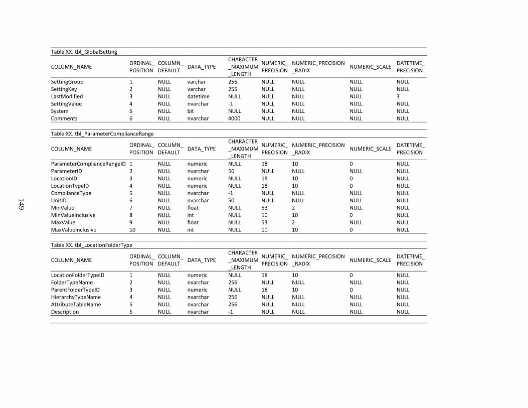
149

Table XX. tbl_GlobalSetting




NUMERIC_PRECISION


PRECISION

SettingGroup 1 NULL varchar 255 NULL NULL NULL NULL SettingKey 2 NULL varchar 255 NULL NULL NULL NULL LastModified 3 NULL datetime NULL NULL NULL NULL 3 SettingValue 4 NULL nvarchar -1 NULL NULL NULL NULL System 5 NULL bit NULL NULL NULL NULL NULL Comments 6 NULL nvarchar 4000 NULL NULL NULL NULL Table XX. tbl_ParameterComplianceRange




NUMERIC_PRECISION


PRECISION

ParameterComplianceRangeID 1 NULL numeric NULL 18 10 0 NULL ParameterID 2 NULL nvarchar 50 NULL NULL NULL NULL LocationID 3 NULL numeric NULL 18 10 0 NULL LocationTypeID 4 NULL numeric NULL 18 10 0 NULL ComplianceType 5 NULL nvarchar -1 NULL NULL NULL NULL UnitID 6 NULL nvarchar 50 NULL NULL NULL NULL MinValue 7 NULL float NULL 53 2 NULL NULL MinValueInclusive 8 NULL int NULL 10 10 0 NULL MaxValue 9 NULL float NULL 53 2 NULL NULL MaxValueInclusive 10 NULL int NULL 10 10 0 NULL Table XX. tbl_LocationFolderType




NUMERIC_PRECISION


PRECISION

LocationFolderTypeID 1 NULL numeric NULL 18 10 0 NULL FolderTypeName 2 NULL nvarchar 256 NULL NULL NULL NULL ParentFolderTypeID 3 NULL numeric NULL 18 10 0 NULL HierarchyTypeName 4 NULL nvarchar 256 NULL NULL NULL NULL AttributeTableName 5 NULL nvarchar 256 NULL NULL NULL NULL Description 6 NULL nvarchar -1 NULL NULL NULL NULL

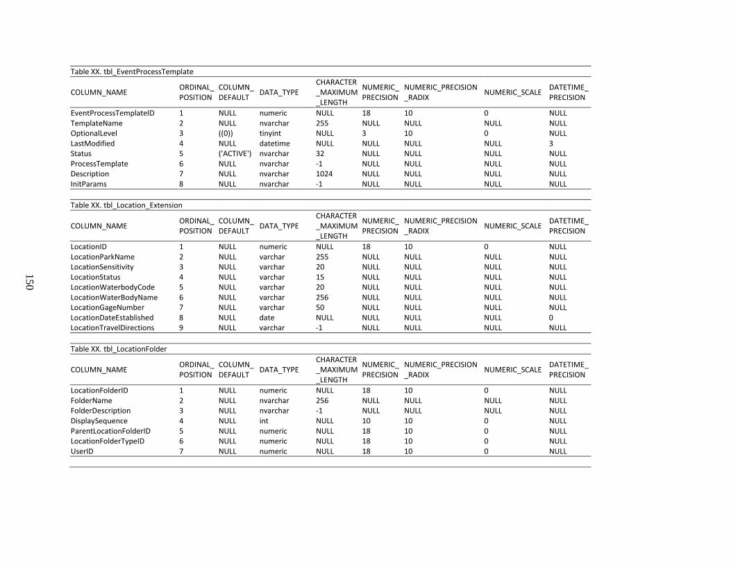
150

Table XX. tbl_EventProcessTemplate




NUMERIC_PRECISION


PRECISION

EventProcessTemplateID 1 NULL numeric NULL 18 10 0 NULL TemplateName 2 NULL nvarchar 255 NULL NULL NULL NULL OptionalLevel 3 ((0)) tinyint NULL 3 10 0 NULL LastModified 4 NULL datetime NULL NULL NULL NULL 3 Status 5 ('ACTIVE') nvarchar 32 NULL NULL NULL NULL ProcessTemplate 6 NULL nvarchar -1 NULL NULL NULL NULL Description 7 NULL nvarchar 1024 NULL NULL NULL NULL InitParams 8 NULL nvarchar -1 NULL NULL NULL NULL Table XX. tbl_Location_Extension




NUMERIC_PRECISION


PRECISION

LocationID 1 NULL numeric NULL 18 10 0 NULL LocationParkName 2 NULL varchar 255 NULL NULL NULL NULL LocationSensitivity 3 NULL varchar 20 NULL NULL NULL NULL LocationStatus 4 NULL varchar 15 NULL NULL NULL NULL LocationWaterbodyCode 5 NULL varchar 20 NULL NULL NULL NULL LocationWaterBodyName 6 NULL varchar 256 NULL NULL NULL NULL LocationGageNumber 7 NULL varchar 50 NULL NULL NULL NULL LocationDateEstablished 8 NULL date NULL NULL NULL NULL 0 LocationTravelDirections 9 NULL varchar -1 NULL NULL NULL NULL Table XX. tbl_LocationFolder




NUMERIC_PRECISION


PRECISION

LocationFolderID 1 NULL numeric NULL 18 10 0 NULL FolderName 2 NULL nvarchar 256 NULL NULL NULL NULL FolderDescription 3 NULL nvarchar -1 NULL NULL NULL NULL DisplaySequence 4 NULL int NULL 10 10 0 NULL ParentLocationFolderID 5 NULL numeric NULL 18 10 0 NULL LocationFolderTypeID 6 NULL numeric NULL 18 10 0 NULL UserID 7 NULL numeric NULL 18 10 0 NULL

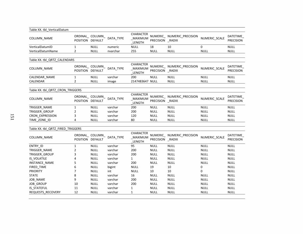
151

Table XX. tbl_VerticalDatum




NUMERIC_PRECISION


PRECISION

VerticalDatumID 1 NULL numeric NULL 18 10 0 NULL VerticalDatumName 2 NULL nvarchar 255 NULL NULL NULL NULL Table XX. tbl_QRTZ_CALENDARS




NUMERIC_PRECISION


PRECISION

CALENDAR_NAME 1 NULL varchar 200 NULL NULL NULL NULL CALENDAR 2 NULL image 2147483647 NULL NULL NULL NULL Table XX. tbl_QRTZ_CRON_TRIGGERS




NUMERIC_PRECISION


PRECISION

TRIGGER_NAME 1 NULL varchar 200 NULL NULL NULL NULL TRIGGER_GROUP 2 NULL varchar 200 NULL NULL NULL NULL CRON_EXPRESSION 3 NULL varchar 120 NULL NULL NULL NULL TIME_ZONE_ID 4 NULL varchar 80 NULL NULL NULL NULL Table XX. tbl_QRTZ_FIRED_TRIGGERS




NUMERIC_PRECISION


PRECISION

ENTRY_ID 1 NULL varchar 95 NULL NULL NULL NULL TRIGGER_NAME 2 NULL varchar 200 NULL NULL NULL NULL TRIGGER_GROUP 3 NULL varchar 200 NULL NULL NULL NULL IS_VOLATILE 4 NULL varchar 1 NULL NULL NULL NULL INSTANCE_NAME 5 NULL varchar 200 NULL NULL NULL NULL FIRED_TIME 6 NULL bigint NULL 19 10 0 NULL PRIORITY 7 NULL int NULL 10 10 0 NULL STATE 8 NULL varchar 16 NULL NULL NULL NULL JOB_NAME 9 NULL varchar 200 NULL NULL NULL NULL JOB_GROUP 10 NULL varchar 200 NULL NULL NULL NULL IS_STATEFUL 11 NULL varchar 1 NULL NULL NULL NULL REQUESTS_RECOVERY 12 NULL varchar 1 NULL NULL NULL NULL

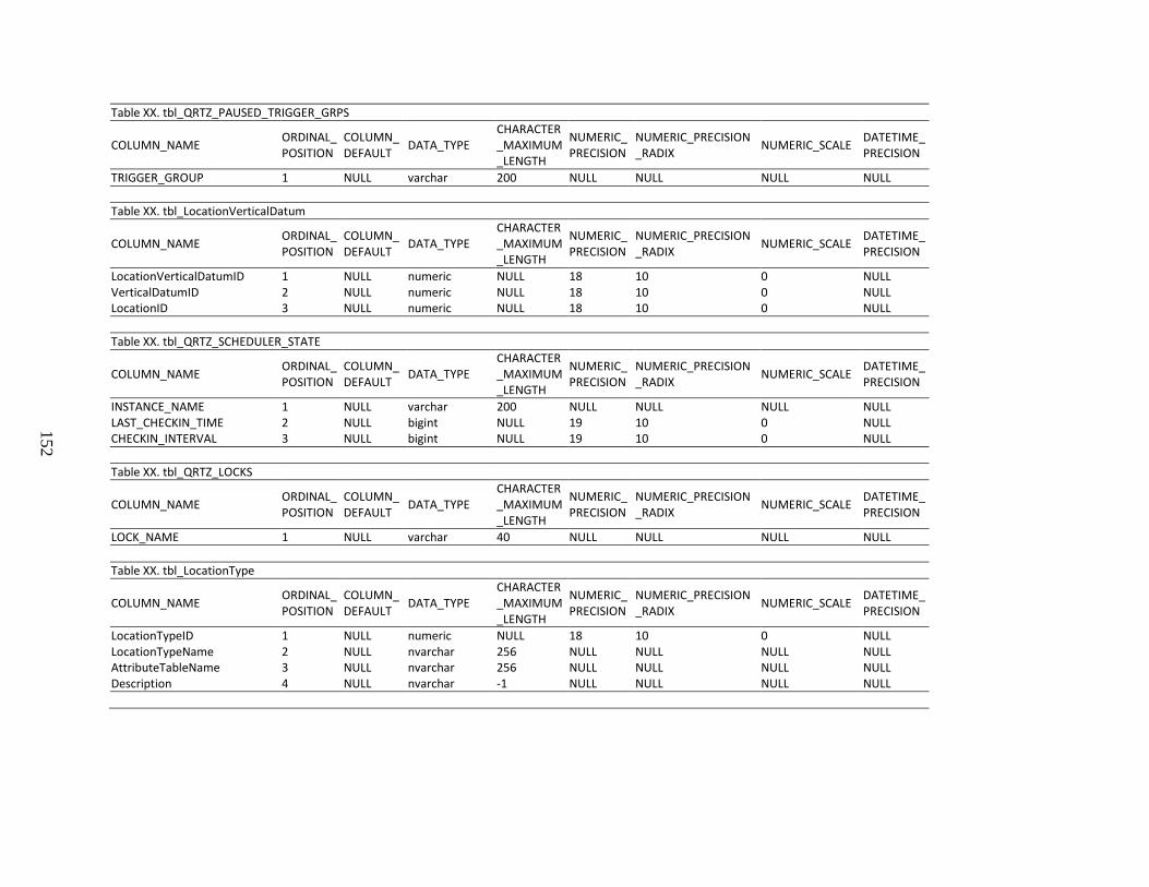
152

Table XX. tbl_QRTZ_PAUSED_TRIGGER_GRPS




NUMERIC_PRECISION


PRECISION

TRIGGER_GROUP 1 NULL varchar 200 NULL NULL NULL NULL Table XX. tbl_LocationVerticalDatum




NUMERIC_PRECISION


PRECISION

LocationVerticalDatumID 1 NULL numeric NULL 18 10 0 NULL VerticalDatumID 2 NULL numeric NULL 18 10 0 NULL LocationID 3 NULL numeric NULL 18 10 0 NULL Table XX. tbl_QRTZ_SCHEDULER_STATE




NUMERIC_PRECISION


PRECISION

INSTANCE_NAME 1 NULL varchar 200 NULL NULL NULL NULL LAST_CHECKIN_TIME 2 NULL bigint NULL 19 10 0 NULL CHECKIN_INTERVAL 3 NULL bigint NULL 19 10 0 NULL Table XX. tbl_QRTZ_LOCKS




NUMERIC_PRECISION


PRECISION

LOCK_NAME 1 NULL varchar 40 NULL NULL NULL NULL Table XX. tbl_LocationType




NUMERIC_PRECISION


PRECISION

LocationTypeID 1 NULL numeric NULL 18 10 0 NULL LocationTypeName 2 NULL nvarchar 256 NULL NULL NULL NULL AttributeTableName 3 NULL nvarchar 256 NULL NULL NULL NULL Description 4 NULL nvarchar -1 NULL NULL NULL NULL

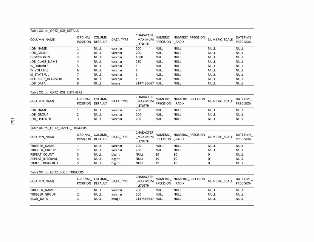
153

Table XX. tbl_QRTZ_JOB_DETAILS




NUMERIC_PRECISION


PRECISION

JOB_NAME 1 NULL varchar 200 NULL NULL NULL NULL JOB_GROUP 2 NULL varchar 200 NULL NULL NULL NULL DESCRIPTION 3 NULL varchar 1000 NULL NULL NULL NULL JOB_CLASS_NAME 4 NULL varchar 250 NULL NULL NULL NULL IS_DURABLE 5 NULL varchar 1 NULL NULL NULL NULL IS_VOLATILE 6 NULL varchar 1 NULL NULL NULL NULL IS_STATEFUL 7 NULL varchar 1 NULL NULL NULL NULL REQUESTS_RECOVERY 8 NULL varchar 1 NULL NULL NULL NULL JOB_DATA 9 NULL image 2147483647 NULL NULL NULL NULL Table XX. tbl_QRTZ_JOB_LISTENERS




NUMERIC_PRECISION


PRECISION

JOB_NAME 1 NULL varchar 200 NULL NULL NULL NULL JOB_GROUP 2 NULL varchar 200 NULL NULL NULL NULL JOB_LISTENER 3 NULL varchar 200 NULL NULL NULL NULL Table XX. tbl_QRTZ_SIMPLE_TRIGGERS




NUMERIC_PRECISION


PRECISION

TRIGGER_NAME 1 NULL varchar 200 NULL NULL NULL NULL TRIGGER_GROUP 2 NULL varchar 200 NULL NULL NULL NULL REPEAT_COUNT 3 NULL bigint NULL 19 10 0 NULL REPEAT_INTERVAL 4 NULL bigint NULL 19 10 0 NULL TIMES_TRIGGERED 5 NULL bigint NULL 19 10 0 NULL Table XX. tbl_QRTZ_BLOB_TRIGGERS




NUMERIC_PRECISION


PRECISION

TRIGGER_NAME 1 NULL varchar 200 NULL NULL NULL NULL TRIGGER_GROUP 2 NULL varchar 200 NULL NULL NULL NULL BLOB_DATA 3 NULL image 2147483647 NULL NULL NULL NULL

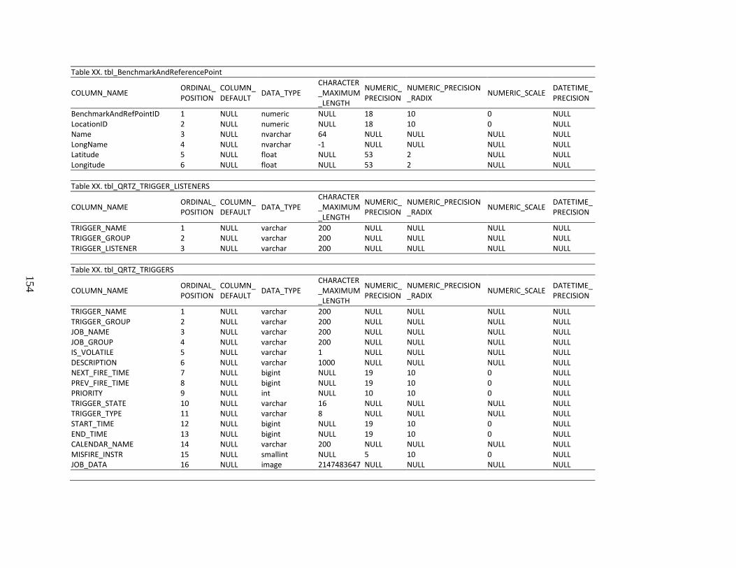
154

Table XX. tbl_BenchmarkAndReferencePoint




NUMERIC_PRECISION


PRECISION

BenchmarkAndRefPointID 1 NULL numeric NULL 18 10 0 NULL LocationID 2 NULL numeric NULL 18 10 0 NULL Name 3 NULL nvarchar 64 NULL NULL NULL NULL LongName 4 NULL nvarchar -1 NULL NULL NULL NULL Latitude 5 NULL float NULL 53 2 NULL NULL Longitude 6 NULL float NULL 53 2 NULL NULL Table XX. tbl_QRTZ_TRIGGER_LISTENERS




NUMERIC_PRECISION


PRECISION

TRIGGER_NAME 1 NULL varchar 200 NULL NULL NULL NULL TRIGGER_GROUP 2 NULL varchar 200 NULL NULL NULL NULL TRIGGER_LISTENER 3 NULL varchar 200 NULL NULL NULL NULL Table XX. tbl_QRTZ_TRIGGERS




NUMERIC_PRECISION


PRECISION

TRIGGER_NAME 1 NULL varchar 200 NULL NULL NULL NULL TRIGGER_GROUP 2 NULL varchar 200 NULL NULL NULL NULL JOB_NAME 3 NULL varchar 200 NULL NULL NULL NULL JOB_GROUP 4 NULL varchar 200 NULL NULL NULL NULL IS_VOLATILE 5 NULL varchar 1 NULL NULL NULL NULL DESCRIPTION 6 NULL varchar 1000 NULL NULL NULL NULL NEXT_FIRE_TIME 7 NULL bigint NULL 19 10 0 NULL PREV_FIRE_TIME 8 NULL bigint NULL 19 10 0 NULL PRIORITY 9 NULL int NULL 10 10 0 NULL TRIGGER_STATE 10 NULL varchar 16 NULL NULL NULL NULL TRIGGER_TYPE 11 NULL varchar 8 NULL NULL NULL NULL START_TIME 12 NULL bigint NULL 19 10 0 NULL END_TIME 13 NULL bigint NULL 19 10 0 NULL CALENDAR_NAME 14 NULL varchar 200 NULL NULL NULL NULL MISFIRE_INSTR 15 NULL smallint NULL 5 10 0 NULL JOB_DATA 16 NULL image 2147483647 NULL NULL NULL NULL

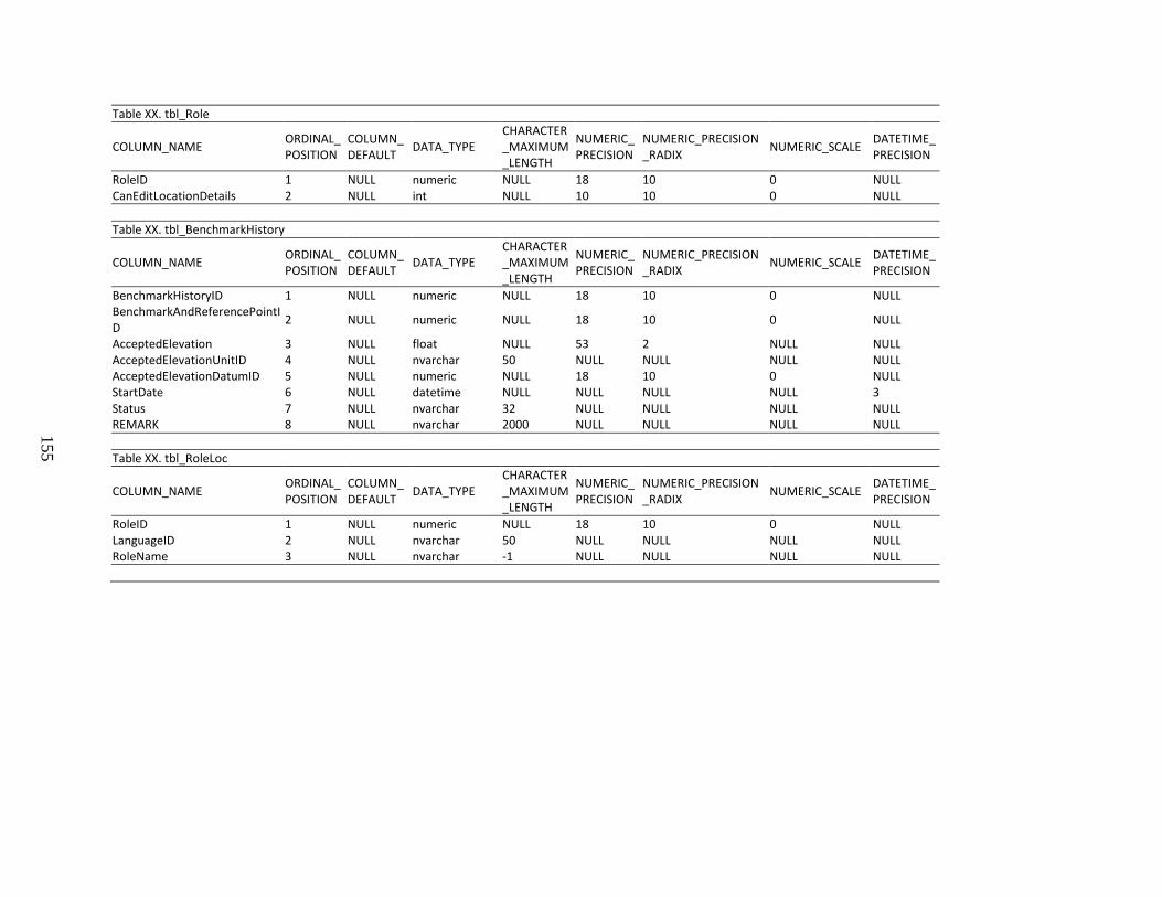
155

Table XX. tbl_Role




NUMERIC_PRECISION


PRECISION

RoleID 1 NULL numeric NULL 18 10 0 NULL CanEditLocationDetails 2 NULL int NULL 10 10 0 NULL Table XX. tbl_BenchmarkHistory




NUMERIC_PRECISION


PRECISION

BenchmarkHistoryID 1 NULL numeric NULL 18 10 0 NULL BenchmarkAndReferencePointID 2 NULL numeric NULL 18 10 0 NULL

AcceptedElevation 3 NULL float NULL 53 2 NULL NULL AcceptedElevationUnitID 4 NULL nvarchar 50 NULL NULL NULL NULL AcceptedElevationDatumID 5 NULL numeric NULL 18 10 0 NULL StartDate 6 NULL datetime NULL NULL NULL NULL 3 Status 7 NULL nvarchar 32 NULL NULL NULL NULL REMARK 8 NULL nvarchar 2000 NULL NULL NULL NULL Table XX. tbl_RoleLoc




NUMERIC_PRECISION


PRECISION

RoleID 1 NULL numeric NULL 18 10 0 NULL LanguageID 2 NULL nvarchar 50 NULL NULL NULL NULL RoleName 3 NULL nvarchar -1 NULL NULL NULL NULL

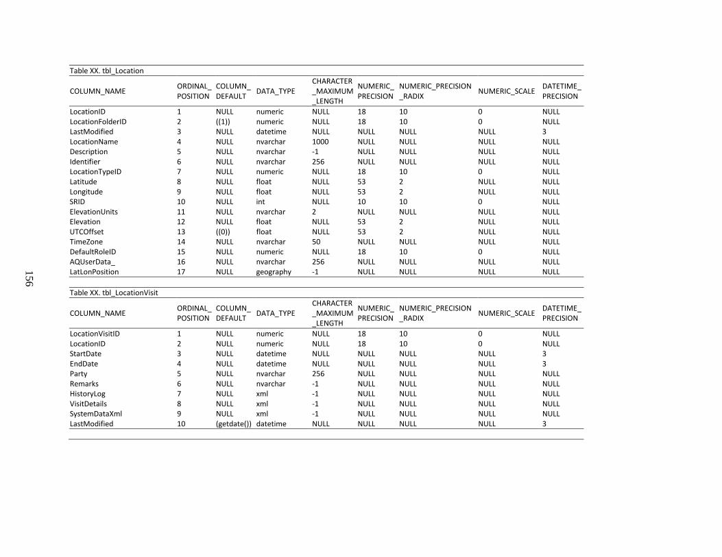
156

Table XX. tbl_Location




NUMERIC_PRECISION


PRECISION

LocationID 1 NULL numeric NULL 18 10 0 NULL LocationFolderID 2 ((1)) numeric NULL 18 10 0 NULL LastModified 3 NULL datetime NULL NULL NULL NULL 3 LocationName 4 NULL nvarchar 1000 NULL NULL NULL NULL Description 5 NULL nvarchar -1 NULL NULL NULL NULL Identifier 6 NULL nvarchar 256 NULL NULL NULL NULL LocationTypeID 7 NULL numeric NULL 18 10 0 NULL Latitude 8 NULL float NULL 53 2 NULL NULL Longitude 9 NULL float NULL 53 2 NULL NULL SRID 10 NULL int NULL 10 10 0 NULL ElevationUnits 11 NULL nvarchar 2 NULL NULL NULL NULL Elevation 12 NULL float NULL 53 2 NULL NULL UTCOffset 13 ((0)) float NULL 53 2 NULL NULL TimeZone 14 NULL nvarchar 50 NULL NULL NULL NULL DefaultRoleID 15 NULL numeric NULL 18 10 0 NULL AQUserData_ 16 NULL nvarchar 256 NULL NULL NULL NULL LatLonPosition 17 NULL geography -1 NULL NULL NULL NULL Table XX. tbl_LocationVisit




NUMERIC_PRECISION


PRECISION

LocationVisitID 1 NULL numeric NULL 18 10 0 NULL LocationID 2 NULL numeric NULL 18 10 0 NULL StartDate 3 NULL datetime NULL NULL NULL NULL 3 EndDate 4 NULL datetime NULL NULL NULL NULL 3 Party 5 NULL nvarchar 256 NULL NULL NULL NULL Remarks 6 NULL nvarchar -1 NULL NULL NULL NULL HistoryLog 7 NULL xml -1 NULL NULL NULL NULL VisitDetails 8 NULL xml -1 NULL NULL NULL NULL SystemDataXml 9 NULL xml -1 NULL NULL NULL NULL LastModified 10 (getdate()) datetime NULL NULL NULL NULL 3

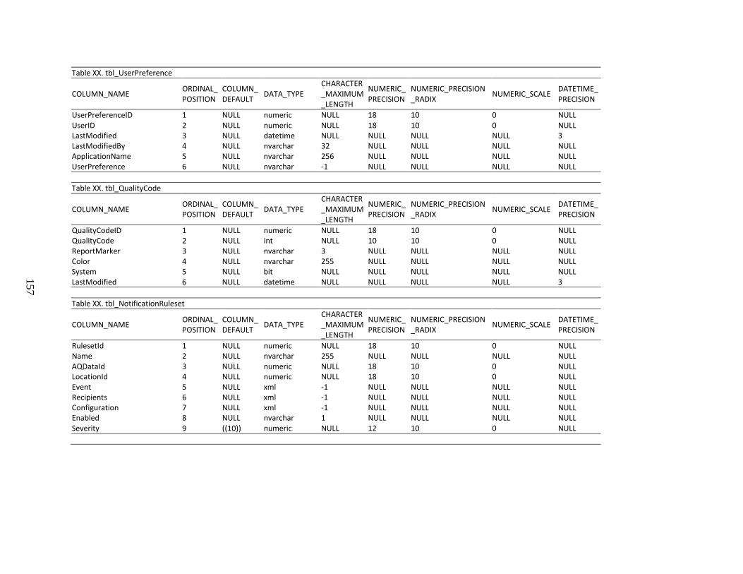
157

Table XX. tbl_UserPreference




NUMERIC_PRECISION


PRECISION

UserPreferenceID 1 NULL numeric NULL 18 10 0 NULL UserID 2 NULL numeric NULL 18 10 0 NULL LastModified 3 NULL datetime NULL NULL NULL NULL 3 LastModifiedBy 4 NULL nvarchar 32 NULL NULL NULL NULL ApplicationName 5 NULL nvarchar 256 NULL NULL NULL NULL UserPreference 6 NULL nvarchar -1 NULL NULL NULL NULL Table XX. tbl_QualityCode




NUMERIC_PRECISION


PRECISION

QualityCodeID 1 NULL numeric NULL 18 10 0 NULL QualityCode 2 NULL int NULL 10 10 0 NULL ReportMarker 3 NULL nvarchar 3 NULL NULL NULL NULL Color 4 NULL nvarchar 255 NULL NULL NULL NULL System 5 NULL bit NULL NULL NULL NULL NULL LastModified 6 NULL datetime NULL NULL NULL NULL 3 Table XX. tbl_NotificationRuleset




NUMERIC_PRECISION


PRECISION

RulesetId 1 NULL numeric NULL 18 10 0 NULL Name 2 NULL nvarchar 255 NULL NULL NULL NULL AQDataId 3 NULL numeric NULL 18 10 0 NULL LocationId 4 NULL numeric NULL 18 10 0 NULL Event 5 NULL xml -1 NULL NULL NULL NULL Recipients 6 NULL xml -1 NULL NULL NULL NULL Configuration 7 NULL xml -1 NULL NULL NULL NULL Enabled 8 NULL nvarchar 1 NULL NULL NULL NULL Severity 9 ((10)) numeric NULL 12 10 0 NULL

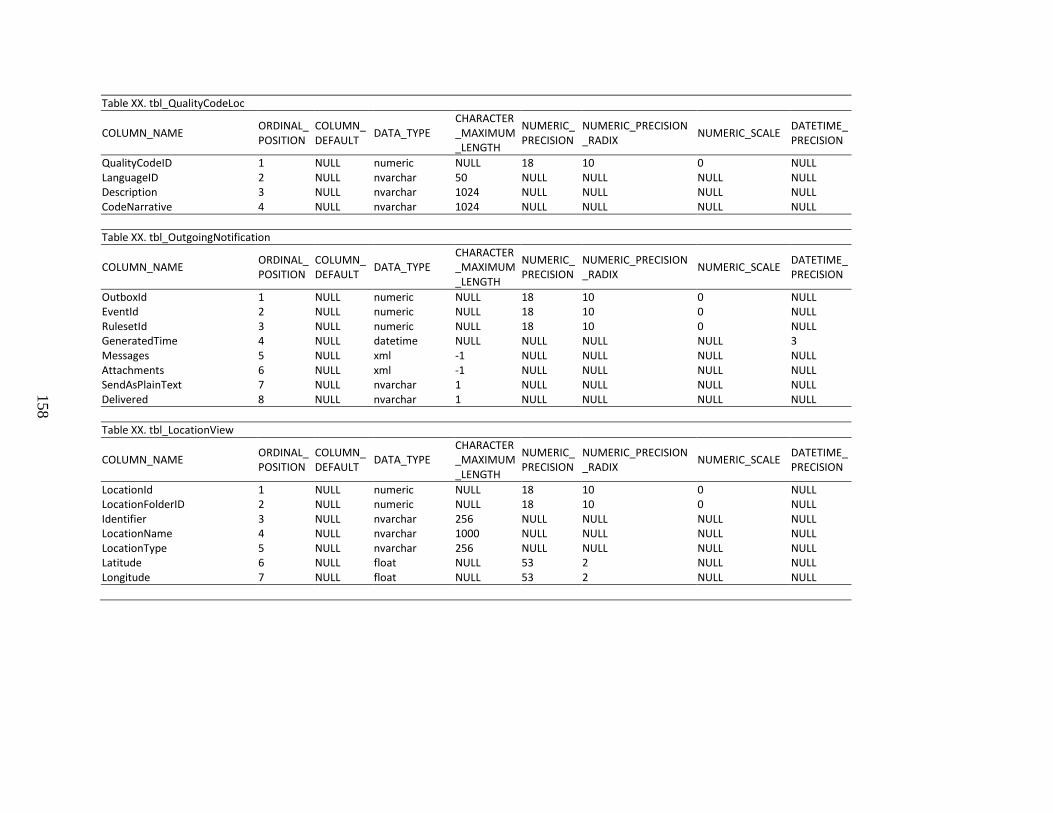
158

Table XX. tbl_QualityCodeLoc




NUMERIC_PRECISION


PRECISION

QualityCodeID 1 NULL numeric NULL 18 10 0 NULL LanguageID 2 NULL nvarchar 50 NULL NULL NULL NULL Description 3 NULL nvarchar 1024 NULL NULL NULL NULL CodeNarrative 4 NULL nvarchar 1024 NULL NULL NULL NULL Table XX. tbl_OutgoingNotification




NUMERIC_PRECISION


PRECISION

OutboxId 1 NULL numeric NULL 18 10 0 NULL EventId 2 NULL numeric NULL 18 10 0 NULL RulesetId 3 NULL numeric NULL 18 10 0 NULL GeneratedTime 4 NULL datetime NULL NULL NULL NULL 3 Messages 5 NULL xml -1 NULL NULL NULL NULL Attachments 6 NULL xml -1 NULL NULL NULL NULL SendAsPlainText 7 NULL nvarchar 1 NULL NULL NULL NULL Delivered 8 NULL nvarchar 1 NULL NULL NULL NULL Table XX. tbl_LocationView




NUMERIC_PRECISION


PRECISION

LocationId 1 NULL numeric NULL 18 10 0 NULL LocationFolderID 2 NULL numeric NULL 18 10 0 NULL Identifier 3 NULL nvarchar 256 NULL NULL NULL NULL LocationName 4 NULL nvarchar 1000 NULL NULL NULL NULL LocationType 5 NULL nvarchar 256 NULL NULL NULL NULL Latitude 6 NULL float NULL 53 2 NULL NULL Longitude 7 NULL float NULL 53 2 NULL NULL

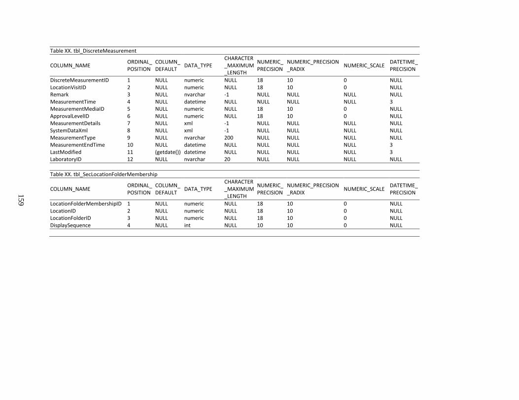
159

Table XX. tbl_DiscreteMeasurement




NUMERIC_PRECISION


PRECISION

DiscreteMeasurementID 1 NULL numeric NULL 18 10 0 NULL LocationVisitID 2 NULL numeric NULL 18 10 0 NULL Remark 3 NULL nvarchar -1 NULL NULL NULL NULL MeasurementTime 4 NULL datetime NULL NULL NULL NULL 3 MeasurementMediaID 5 NULL numeric NULL 18 10 0 NULL ApprovalLevelID 6 NULL numeric NULL 18 10 0 NULL MeasurementDetails 7 NULL xml -1 NULL NULL NULL NULL SystemDataXml 8 NULL xml -1 NULL NULL NULL NULL MeasurementType 9 NULL nvarchar 200 NULL NULL NULL NULL MeasurementEndTime 10 NULL datetime NULL NULL NULL NULL 3 LastModified 11 (getdate()) datetime NULL NULL NULL NULL 3 LaboratoryID 12 NULL nvarchar 20 NULL NULL NULL NULL Table XX. tbl_SecLocationFolderMembership




NUMERIC_PRECISION


PRECISION

LocationFolderMembershipID 1 NULL numeric NULL 18 10 0 NULL LocationID 2 NULL numeric NULL 18 10 0 NULL LocationFolderID 3 NULL numeric NULL 18 10 0 NULL DisplaySequence 4 NULL int NULL 10 10 0 NULL

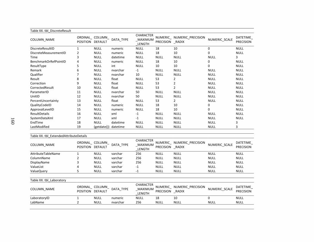
160

Table XX. tbl_DiscreteResult




NUMERIC_PRECISION


PRECISION

DiscreteResultID 1 NULL numeric NULL 18 10 0 NULL DiscreteMeasurementID 2 NULL numeric NULL 18 10 0 NULL Time 3 NULL datetime NULL NULL NULL NULL 3 BenchmarkOrRefPointID 4 NULL numeric NULL 18 10 0 NULL ResultType 5 NULL int NULL 10 10 0 NULL Remark 6 NULL nvarchar -1 NULL NULL NULL NULL Qualifier 7 NULL nvarchar 10 NULL NULL NULL NULL Result 8 NULL float NULL 53 2 NULL NULL Correction 9 NULL float NULL 53 2 NULL NULL CorrectedResult 10 NULL float NULL 53 2 NULL NULL ParameterID 11 NULL nvarchar 50 NULL NULL NULL NULL UnitID 12 NULL nvarchar 50 NULL NULL NULL NULL PercentUncertainty 13 NULL float NULL 53 2 NULL NULL QualityCodeID 14 NULL numeric NULL 18 10 0 NULL ApprovalLevelID 15 NULL numeric NULL 18 10 0 NULL ResultDetails 16 NULL xml -1 NULL NULL NULL NULL SystemDataXml 17 NULL xml -1 NULL NULL NULL NULL EndTime 18 NULL datetime NULL NULL NULL NULL 3 LastModified 19 (getdate()) datetime NULL NULL NULL NULL 3 Table XX. tbl_ExtendedAttributeDetails




NUMERIC_PRECISION


PRECISION

AttributeTableName 1 NULL varchar 256 NULL NULL NULL NULL ColumnName 2 NULL varchar 256 NULL NULL NULL NULL DisplayName 3 NULL varchar 256 NULL NULL NULL NULL ValueList 4 NULL varchar -1 NULL NULL NULL NULL ValueQuery 5 NULL varchar -1 NULL NULL NULL NULL Table XX. tbl_Laboratory




NUMERIC_PRECISION


PRECISION

LaboratoryID 1 NULL numeric NULL 18 10 0 NULL LabName 2 NULL nvarchar 256 NULL NULL NULL NULL

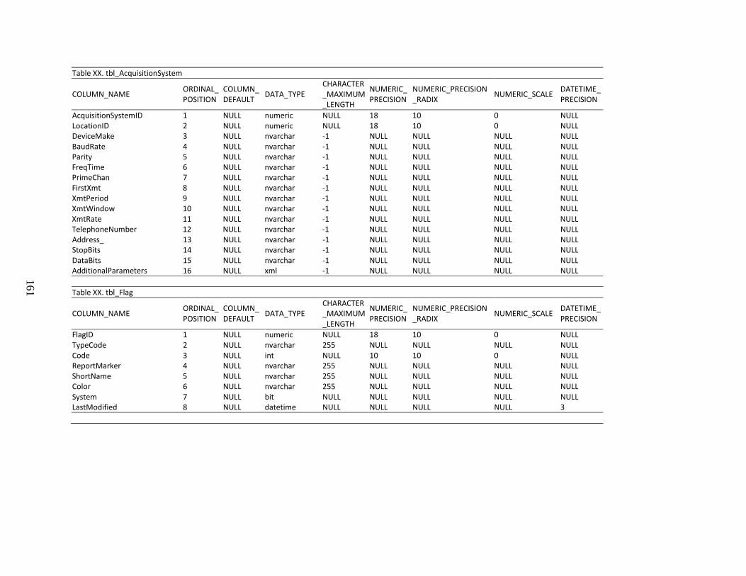
161

Table XX. tbl_AcquisitionSystem




NUMERIC_PRECISION


PRECISION

AcquisitionSystemID 1 NULL numeric NULL 18 10 0 NULL LocationID 2 NULL numeric NULL 18 10 0 NULL DeviceMake 3 NULL nvarchar -1 NULL NULL NULL NULL BaudRate 4 NULL nvarchar -1 NULL NULL NULL NULL Parity 5 NULL nvarchar -1 NULL NULL NULL NULL FreqTime 6 NULL nvarchar -1 NULL NULL NULL NULL PrimeChan 7 NULL nvarchar -1 NULL NULL NULL NULL FirstXmt 8 NULL nvarchar -1 NULL NULL NULL NULL XmtPeriod 9 NULL nvarchar -1 NULL NULL NULL NULL XmtWindow 10 NULL nvarchar -1 NULL NULL NULL NULL XmtRate 11 NULL nvarchar -1 NULL NULL NULL NULL TelephoneNumber 12 NULL nvarchar -1 NULL NULL NULL NULL Address_ 13 NULL nvarchar -1 NULL NULL NULL NULL StopBits 14 NULL nvarchar -1 NULL NULL NULL NULL DataBits 15 NULL nvarchar -1 NULL NULL NULL NULL AdditionalParameters 16 NULL xml -1 NULL NULL NULL NULL Table XX. tbl_Flag




NUMERIC_PRECISION


PRECISION

FlagID 1 NULL numeric NULL 18 10 0 NULL TypeCode 2 NULL nvarchar 255 NULL NULL NULL NULL Code 3 NULL int NULL 10 10 0 NULL ReportMarker 4 NULL nvarchar 255 NULL NULL NULL NULL ShortName 5 NULL nvarchar 255 NULL NULL NULL NULL Color 6 NULL nvarchar 255 NULL NULL NULL NULL System 7 NULL bit NULL NULL NULL NULL NULL LastModified 8 NULL datetime NULL NULL NULL NULL 3

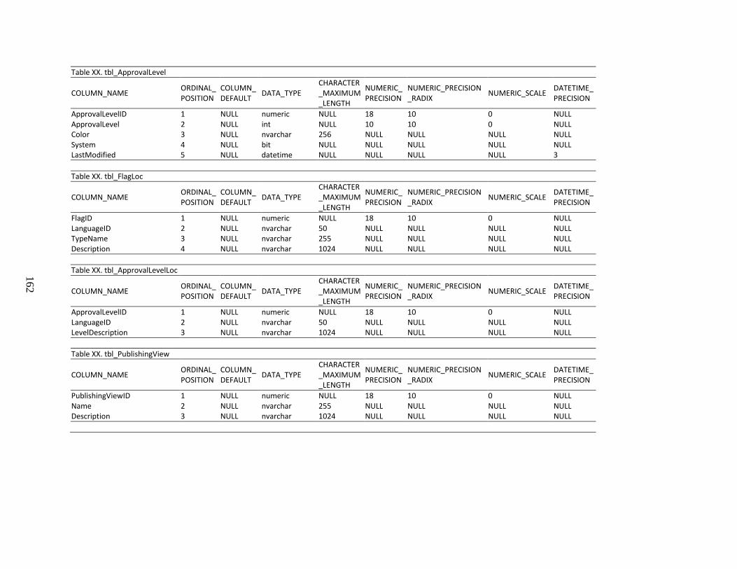
162

Table XX. tbl_ApprovalLevel




NUMERIC_PRECISION


PRECISION

ApprovalLevelID 1 NULL numeric NULL 18 10 0 NULL ApprovalLevel 2 NULL int NULL 10 10 0 NULL Color 3 NULL nvarchar 256 NULL NULL NULL NULL System 4 NULL bit NULL NULL NULL NULL NULL LastModified 5 NULL datetime NULL NULL NULL NULL 3 Table XX. tbl_FlagLoc




NUMERIC_PRECISION


PRECISION

FlagID 1 NULL numeric NULL 18 10 0 NULL LanguageID 2 NULL nvarchar 50 NULL NULL NULL NULL TypeName 3 NULL nvarchar 255 NULL NULL NULL NULL Description 4 NULL nvarchar 1024 NULL NULL NULL NULL Table XX. tbl_ApprovalLevelLoc




NUMERIC_PRECISION


PRECISION

ApprovalLevelID 1 NULL numeric NULL 18 10 0 NULL LanguageID 2 NULL nvarchar 50 NULL NULL NULL NULL LevelDescription 3 NULL nvarchar 1024 NULL NULL NULL NULL Table XX. tbl_PublishingView




NUMERIC_PRECISION


PRECISION

PublishingViewID 1 NULL numeric NULL 18 10 0 NULL Name 2 NULL nvarchar 255 NULL NULL NULL NULL Description 3 NULL nvarchar 1024 NULL NULL NULL NULL

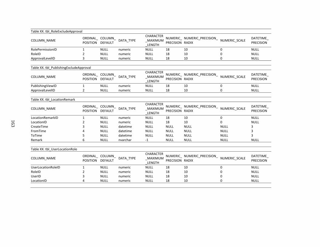
163

Table XX. tbl_RoleExcludeApproval




NUMERIC_PRECISION


PRECISION

RolePermissionID 1 NULL numeric NULL 18 10 0 NULL RoleID 2 NULL numeric NULL 18 10 0 NULL ApprovalLevelID 3 NULL numeric NULL 18 10 0 NULL Table XX. tbl_PublishingExcludeApproval




NUMERIC_PRECISION


PRECISION

PublishingViewID 1 NULL numeric NULL 18 10 0 NULL ApprovalLevelID 2 NULL numeric NULL 18 10 0 NULL Table XX. tbl_LocationRemark




NUMERIC_PRECISION


PRECISION

LocationRemarkID 1 NULL numeric NULL 18 10 0 NULL LocationID 2 NULL numeric NULL 18 10 0 NULL CreateTime 3 NULL datetime NULL NULL NULL NULL 3 FromTime 4 NULL datetime NULL NULL NULL NULL 3 ToTime 5 NULL datetime NULL NULL NULL NULL 3 Remark 6 NULL nvarchar -1 NULL NULL NULL NULL Table XX. tbl_UserLocationRole




NUMERIC_PRECISION


PRECISION

UserLocationRoleID 1 NULL numeric NULL 18 10 0 NULL RoleID 2 NULL numeric NULL 18 10 0 NULL UserID 3 NULL numeric NULL 18 10 0 NULL LocationID 4 NULL numeric NULL 18 10 0 NULL

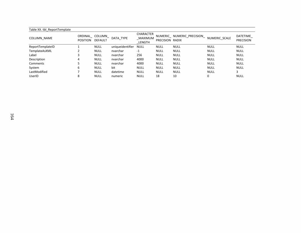
164

Table XX. tbl_ReportTemplate




NUMERIC_PRECISION


PRECISION

ReportTemplateID 1 NULL uniqueidentifier NULL NULL NULL NULL NULL TemplateAsXML 2 NULL nvarchar -1 NULL NULL NULL NULL Label 3 NULL nvarchar 256 NULL NULL NULL NULL Description 4 NULL nvarchar 4000 NULL NULL NULL NULL Comments 5 NULL nvarchar 4000 NULL NULL NULL NULL System 6 NULL bit NULL NULL NULL NULL NULL LastModified 7 NULL datetime NULL NULL NULL NULL 3 UserID 8 NULL numeric NULL 18 10 0 NULL

The Department of the Interior protects and manages the nation’s natural resources and cultural heritage; provides scientific and other information about those resources; and honors its special responsibilities to American Indians, Alaska Natives, and affiliated Island Communities. NPS XXXXXX, March 2012

National Park Service U.S. Department of the Interior

Natural Resource Stewardship and Science 1201 Oakridge Drive, Suite 150 Fort Collins, CO 80525 www.nature.nps.gov

EXPERIENCE YOUR AMERICA TM