Embed Size (px)
DESCRIPTION
application for matlab and simulinksimulinksimulinksimulinksimulinksimulinksimulinksimulinksimulinksimulinksimulinksimulinksimulinksimulinksimulinksimulinksimulinksimulinksimulinksimulinksimulinksimulinksimulinksimulinksimulinksimulinksimulinksimulinksimulinksimulinksimulinksimulinksimulinksimulinksimulinksimulinksimulinksimulinksimulinksimulinksimulinksimulinksimulinksimulinksimulinksimulinksimulinksimulinksimulinksimulinksimulinksimulinksimulinksimulinksimulinksimulinksimulinksimulinksimulinksimulinksimulinksimulinksimulinksimulinksimulinksimulinksimulinksimulinksimulinksimulinksimulinksimulinksimulinksimulinksimulinksimulinksimulinksimulinksimulinksimulinksimulinksimulinksimulinksimulinksimulinksimulinksimulinksimulinksimulinksimulinksimulinksimulinksimulinksimulinksimulinksimulinksimulinksimulinksimulinksimulinksimulinksimulinksimulinksimulinksimulinksimulinksimulinksimulinksimulinksimulinksimulinksimulinksimulinksimulinksimulinksimulink
Citation preview
Signal Processing and Communications
with MATLAB and Simulink
1
Giorgia Zucchelli
Application Engineer - MathWorks
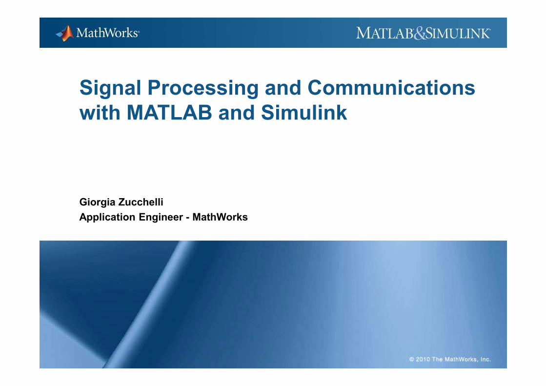
Key Takeaways
� Quickly analyze and develop new algorithms with MATLAB
� Accurate system-level multi-domain analysis with Simulink
2
� Accurate system-level multi-domain analysis with Simulink
� With MATLAB and Simulink you can quickly design entire
systems with better performance
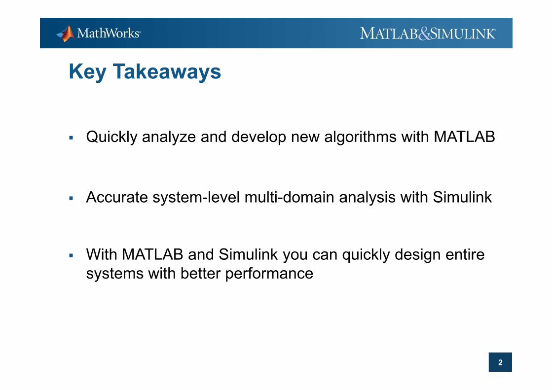
Motivations
� Quickly analyze and develop new algorithms with MATLAB
>> Evaluating innovative ideas is time-consuming
� Accurate system-level multi-domain analysis with Simulink
3
� Accurate system-level multi-domain analysis with Simulink
>> Modeling implementation constraints requires specific knowledge
� With MATLAB and Simulink you can quickly design entire
systems with better performance
>> Optimizing the tradeoff between reuse and innovation is
challenging
MATLAB for Signal Processing
� Digital Filter Design
� Fixed-point in MATLAB
� … and more
4
MATLAB for Signal Processing: What’s New
� Multirate Digital Filter Design
� Fixed-point in MATLAB for streaming applications
� … and more
5
Challenges: Digital Filter Design
� During design:
� Is it meeting the specs?
� During implementation:
� How can I minimize cost?
6
� How can I minimize cost?
� Which filter structure will be optimal?
� Will it work correctly on the target hardware?
� What can I trade off?
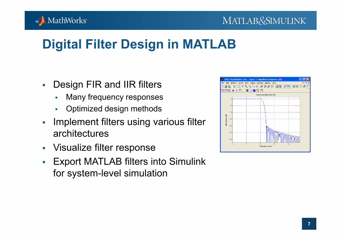
Digital Filter Design in MATLAB
� Design FIR and IIR filters
� Many frequency responses
� Optimized design methods
� Implement filters using various filter
7
� Implement filters using various filter
architectures
� Visualize filter response
� Export MATLAB filters into Simulink
for system-level simulation
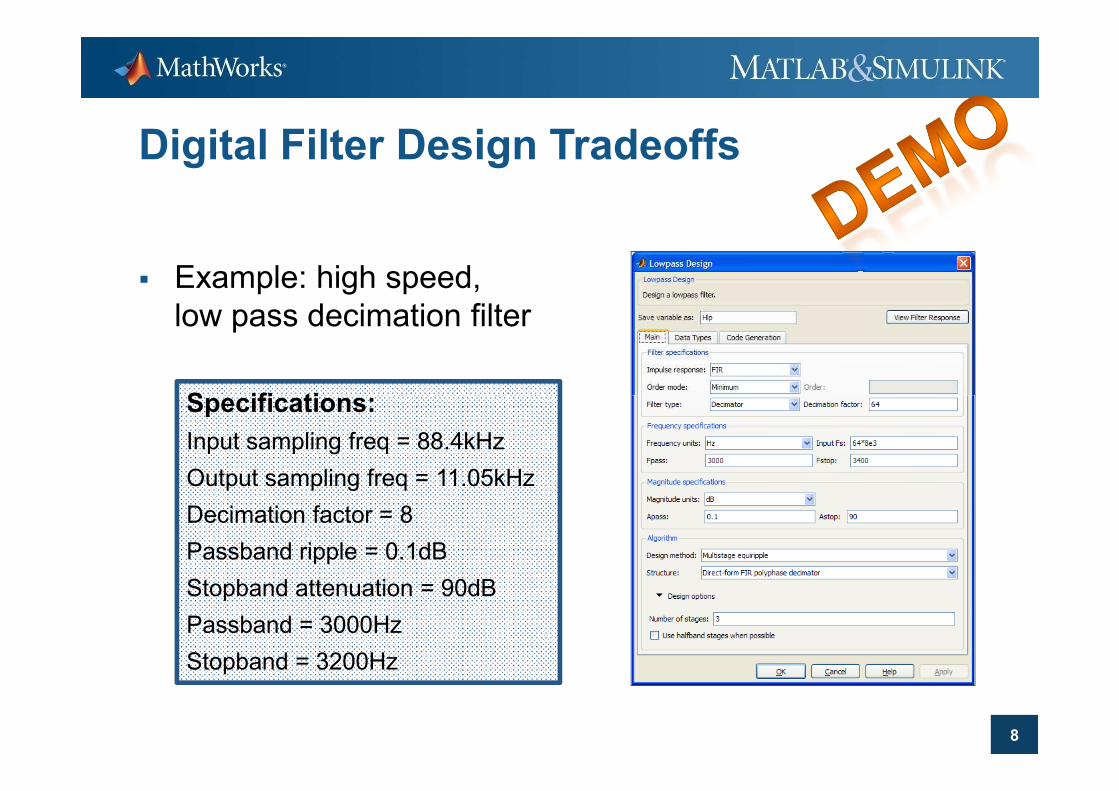
Digital Filter Design Tradeoffs
� Example: high speed,
low pass decimation filter
Specifications:
8
Specifications:
Input sampling freq = 88.4kHz
Output sampling freq = 11.05kHz
Decimation factor = 8
Passband ripple = 0.1dB
Stopband attenuation = 90dB
Passband = 3000Hz
Stopband = 3200Hz
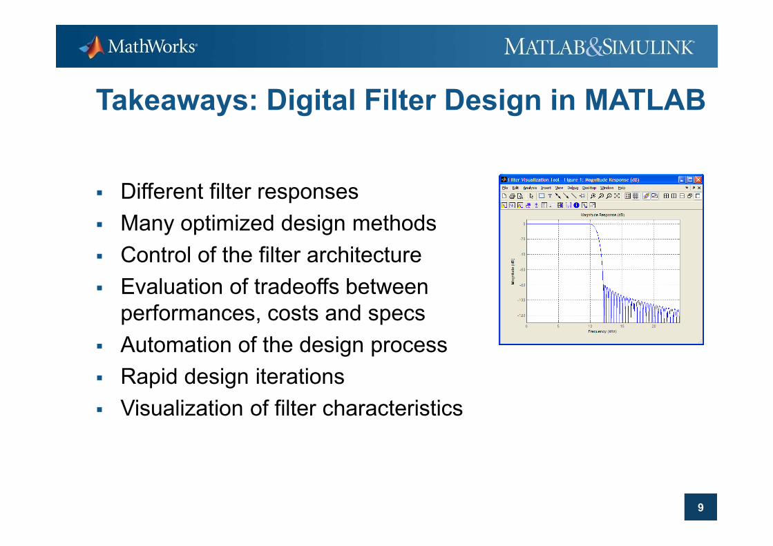
Takeaways: Digital Filter Design in MATLAB
� Different filter responses
� Many optimized design methods
� Control of the filter architecture
9
� Evaluation of tradeoffs between
performances, costs and specs
� Automation of the design process
� Rapid design iterations
� Visualization of filter characteristics
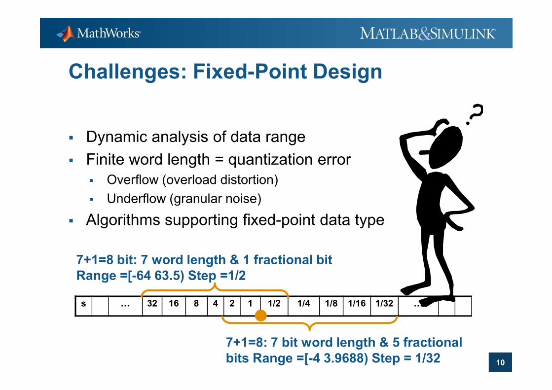
Challenges: Fixed-Point Design
� Dynamic analysis of data range
� Finite word length = quantization error
� Overflow (overload distortion)
� Underflow (granular noise)
10
� Underflow (granular noise)
� Algorithms supporting fixed-point data type
s … 32 16 8 4 2 1 1/2 1/4 1/8 1/16 1/32 …
7+1=8: 7 bit word length & 5 fractional
bits Range =[-4 3.9688) Step = 1/32
7+1=8 bit: 7 word length & 1 fractional bit
Range =[-64 63.5) Step =1/2
MATLAB for Fixed-Point
� Represent fixed-point data type
� Analyze quantization effects
� Built-in logging and visualizations
Accelerate execution of fixed-point code
11
� Accelerate execution of fixed-point code
� System objects for more fixed-point functions
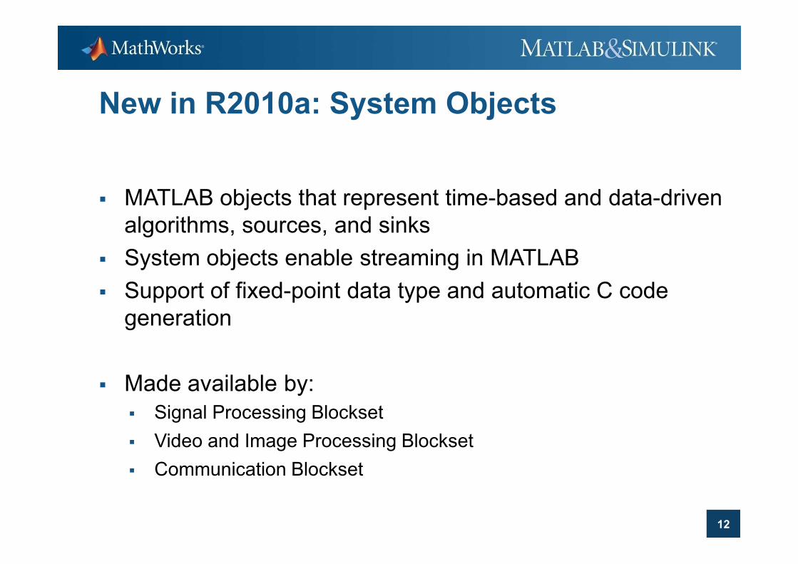
New in R2010a: System Objects
� MATLAB objects that represent time-based and data-driven
algorithms, sources, and sinks
� System objects enable streaming in MATLAB
Support of fixed-point data type and automatic C code
12
� Support of fixed-point data type and automatic C code
generation
� Made available by:
� Signal Processing Blockset
� Video and Image Processing Blockset
� Communication Blockset
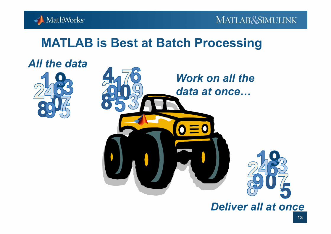
Work on all the
data at once…
MATLAB is Best at Batch Processing
All the data
13
Deliver all at once
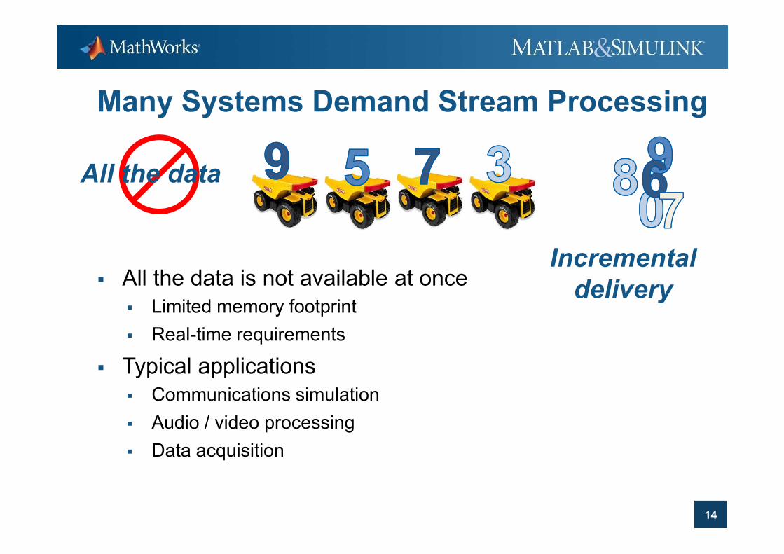
Many Systems Demand Stream Processing
� All the data is not available at onceIncremental
delivery
All the data
14
� All the data is not available at once
� Limited memory footprint
� Real-time requirements
� Typical applications
� Communications simulation
� Audio / video processing
� Data acquisition
delivery
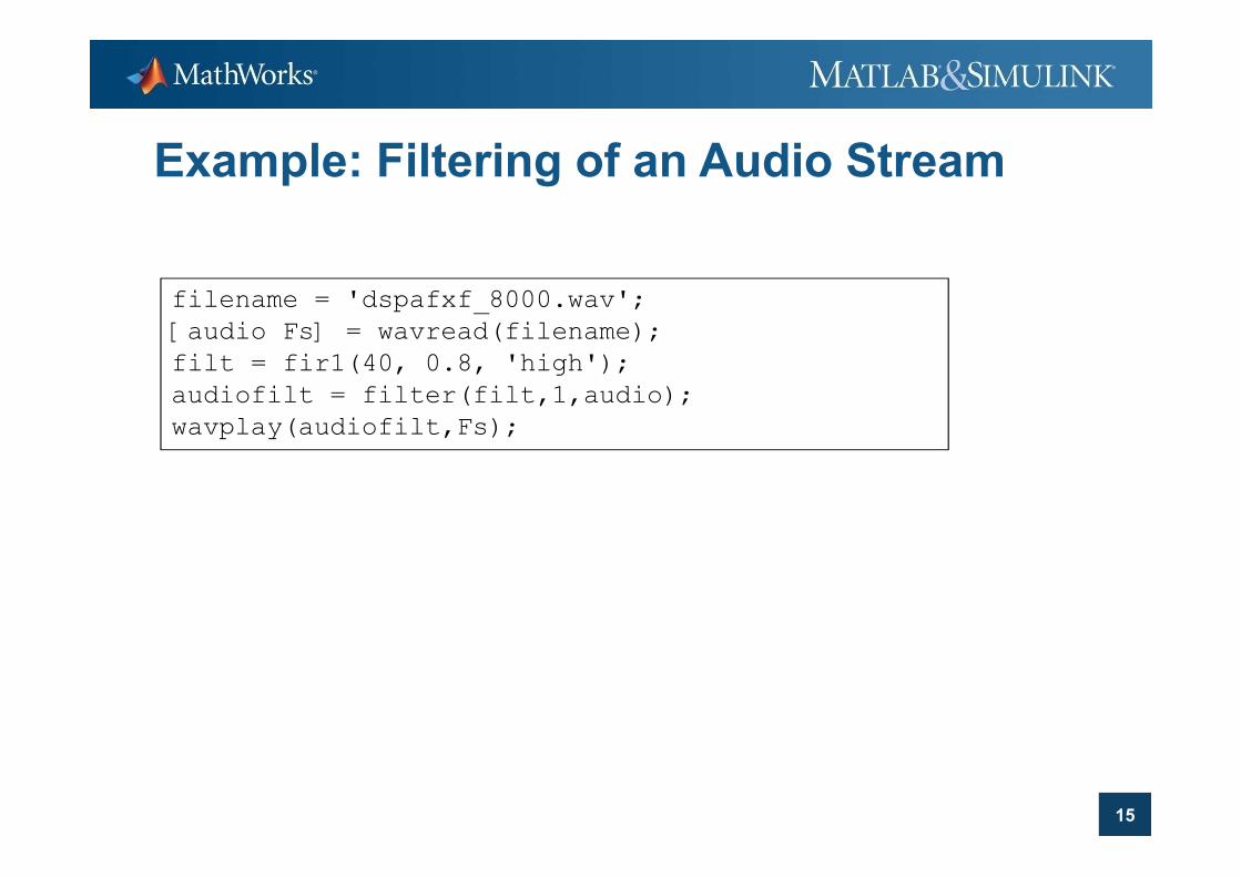
Example: Filtering of an Audio Stream
filename = 'dspafxf_8000.wav';
[audio Fs] = wavread(filename);
filt = fir1(40, 0.8, 'high');
audiofilt = filter(filt,1,audio);
wavplay(audiofilt,Fs);
15
wavplay(audiofilt,Fs);
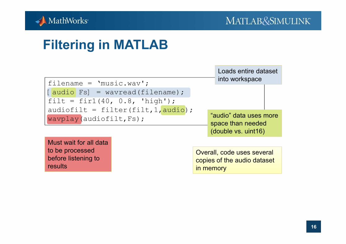
Filtering in MATLAB
filename = ‘music.wav';
[audio Fs] = wavread(filename);
filt = fir1(40, 0.8, 'high');
audiofilt = filter(filt,1,audio);
wavplay(audiofilt,Fs);
Loads entire dataset
into workspace
“audio” data uses more
space than needed
16
Must wait for all data
to be processed
before listening to
results
Overall, code uses several
copies of the audio dataset
in memory
wavplay(audiofilt,Fs);space than needed
(double vs. uint16)
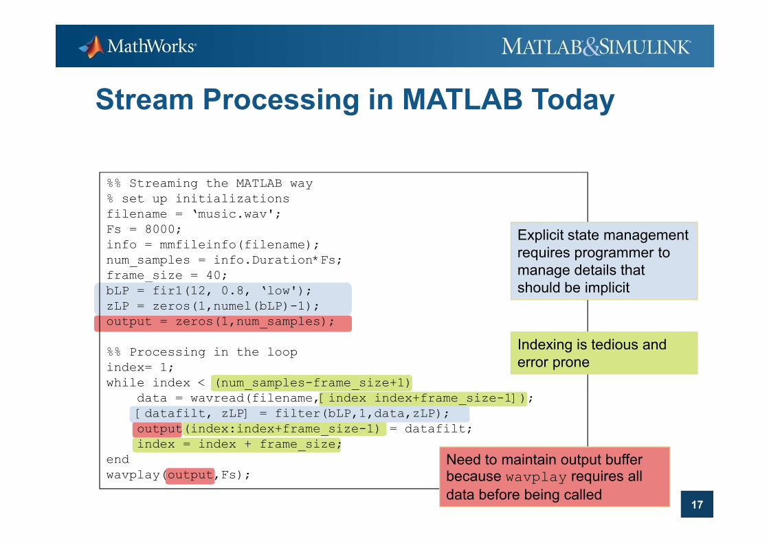
Stream Processing in MATLAB Today
%% Streaming the MATLAB way
% set up initializations
filename = ‘music.wav';
Fs = 8000;
info = mmfileinfo(filename);
num_samples = info.Duration*Fs;
frame_size = 40;
Explicit state management
requires programmer to
manage details that
17
frame_size = 40;
bLP = fir1(12, 0.8, ‘low');
zLP = zeros(1,numel(bLP)-1);
output = zeros(1,num_samples);
%% Processing in the loop
index= 1;
while index < (num_samples-frame_size+1)
data = wavread(filename,[index index+frame_size-1]);
[datafilt, zLP] = filter(bLP,1,data,zLP);
output(index:index+frame_size-1) = datafilt;
index = index + frame_size;
end
wavplay(output,Fs);
manage details that
should be implicit
Indexing is tedious and
error prone
Need to maintain output buffer because wavplay requires all
data before being called
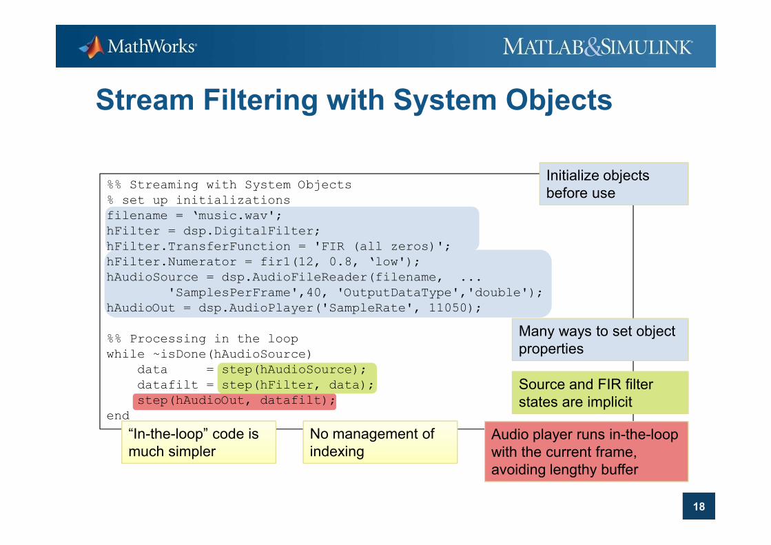
%% Streaming with System Objects
% set up initializations
filename = ‘music.wav';
hFilter = dsp.DigitalFilter;
hFilter.TransferFunction = 'FIR (all zeros)';
hFilter.Numerator = fir1(12, 0.8, ‘low');
hAudioSource = dsp.AudioFileReader(filename, ...
Stream Filtering with System Objects
Initialize objects
before use
18
hAudioSource = dsp.AudioFileReader(filename, ...
'SamplesPerFrame',40, 'OutputDataType','double');
hAudioOut = dsp.AudioPlayer('SampleRate', 11050);
%% Processing in the loop
while ~isDone(hAudioSource)
data = step(hAudioSource);
datafilt = step(hFilter, data);
step(hAudioOut, datafilt);
end
Many ways to set object
properties
Source and FIR filter
states are implicit
“In-the-loop” code is
much simpler
No management of
indexingAudio player runs in-the-loop
with the current frame,
avoiding lengthy buffer
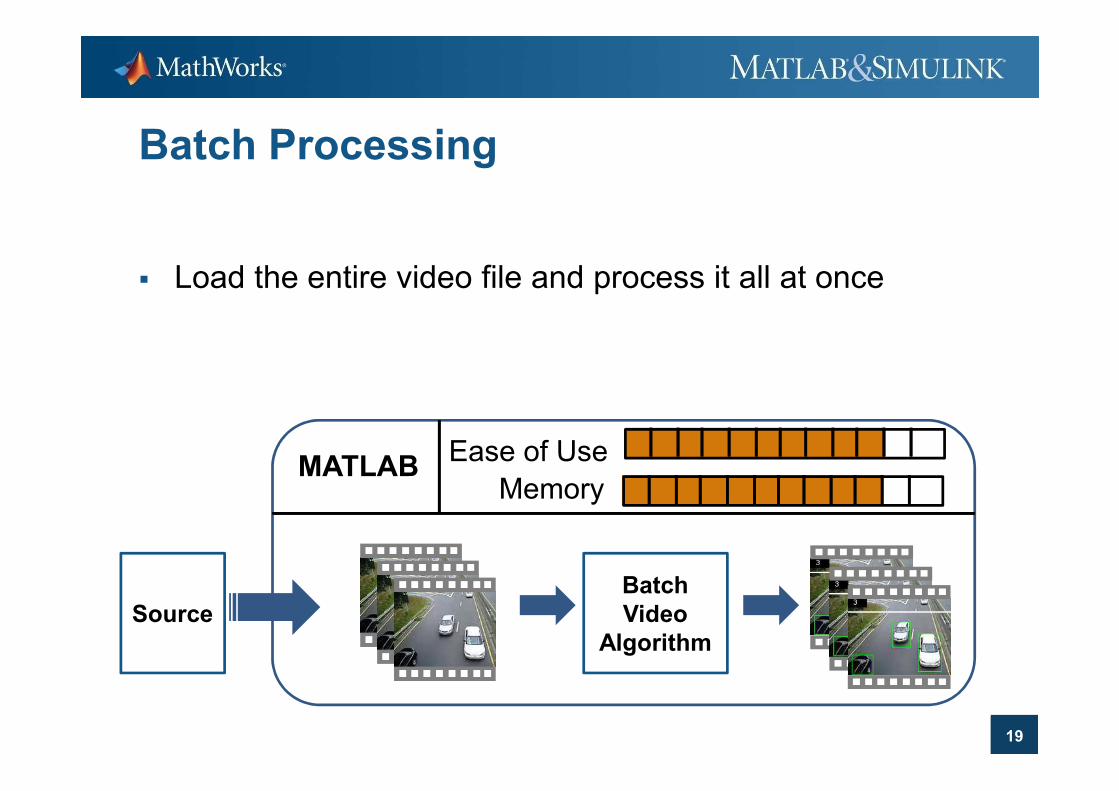
Batch Processing
� Load the entire video file and process it all at once
191919
Source
Batch
Video
Algorithm
Memory
Ease of UseMATLAB
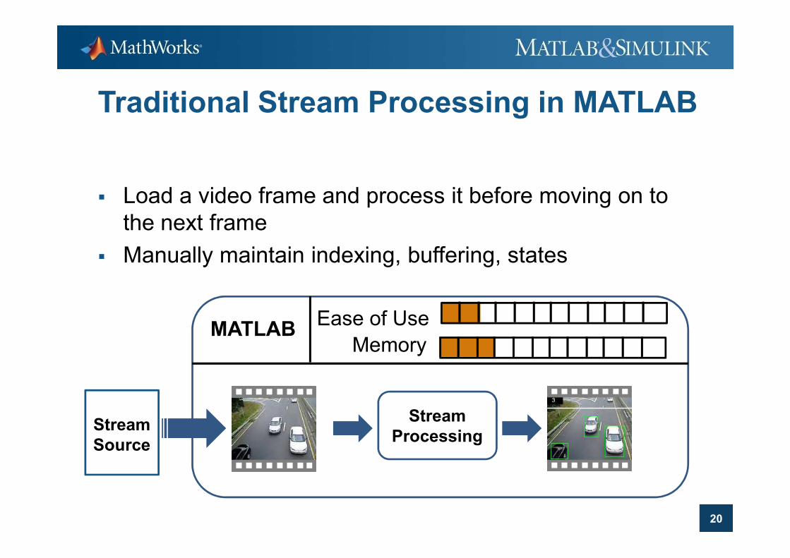
Traditional Stream Processing in MATLAB
� Load a video frame and process it before moving on to
the next frame
� Manually maintain indexing, buffering, states
20
MATLAB
Stream
ProcessingStream
Source
Ease of Use
Memory
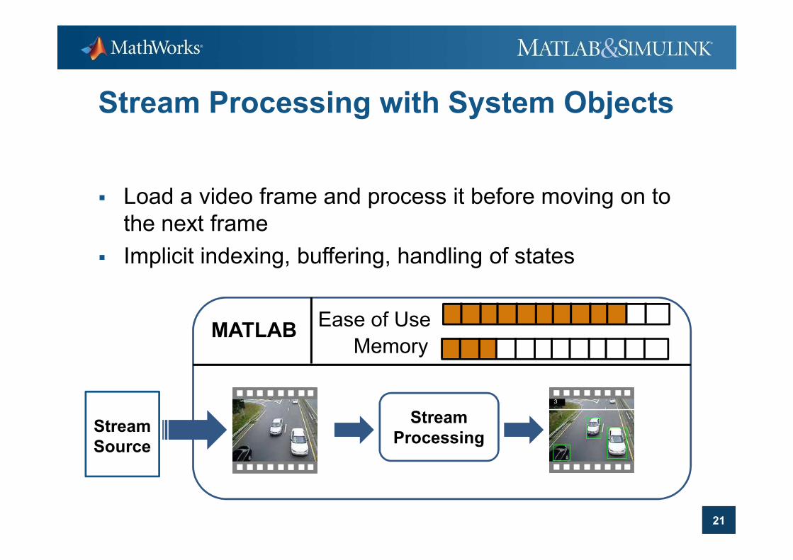
Stream Processing with System Objects
� Load a video frame and process it before moving on to
the next frame
� Implicit indexing, buffering, handling of states
21
MATLAB
Stream
ProcessingStream
Source
Ease of Use
Memory
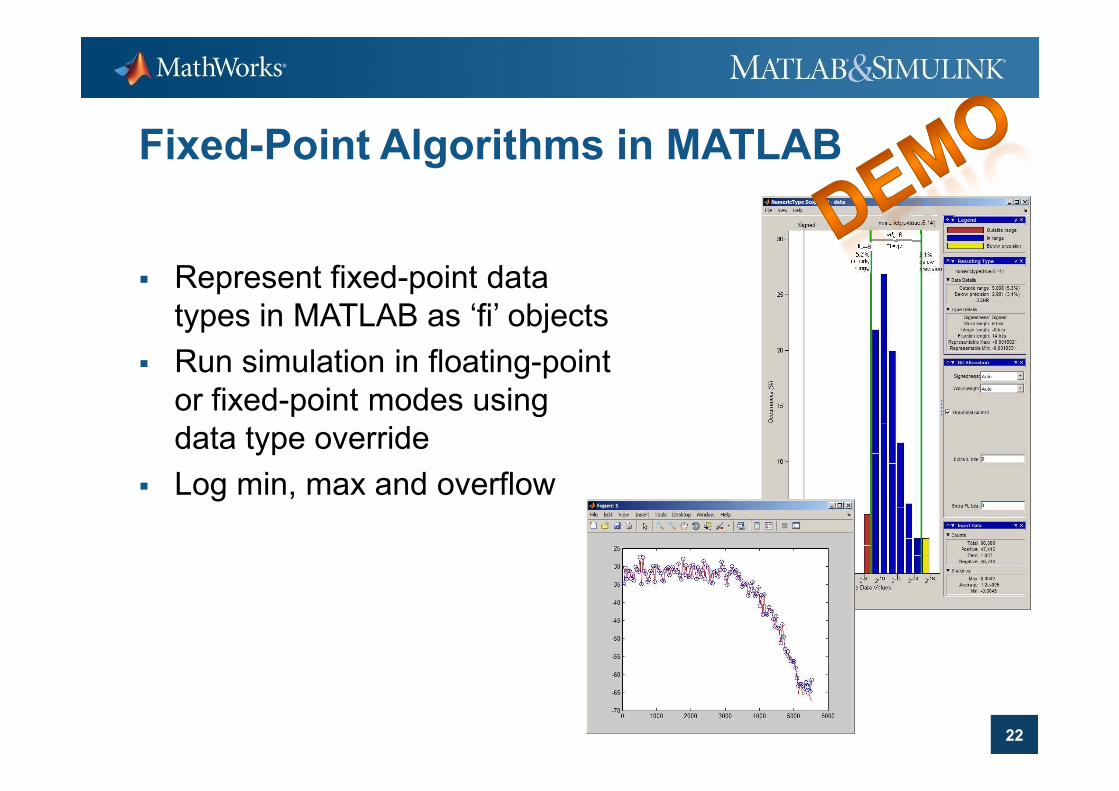
Fixed-Point Algorithms in MATLAB
� Represent fixed-point data
types in MATLAB as ‘fi’ objects
� Run simulation in floating-point
or fixed-point modes using
22
or fixed-point modes using
data type override
� Log min, max and overflow
Takeaways: Fixed-Point System Objects
� Stream processing in MATLAB
� Easier to write and be correct the first time
� Improves handling of large data sets
� Fixed-point modeling
23
� Fixed-point modeling
� All relevant objects support fixed-point data types
� Compatible with Fixed-Point Toolbox
� C-code generation
� Most objects support code generation using EMLC
� Compatible with Embedded MATLAB
Simulink for Signal Processing
� Systems with complex timing
� System-level simulation
� … and more
24
Simulink for Signal Processing: What’s New
� Mixed-signal systems with complex timing
� System-level simulation including RF
� … and more
25
Challenges: Mixed-Signal Systems
� Anticipate physical constraints� Analog and digital electronics
� Complex timing:� Continuous and discrete timing
26
� Continuous and discrete timing
� Feedback loops
� Threshold crossing
� Asynchronous behavior
� Concurrent paths
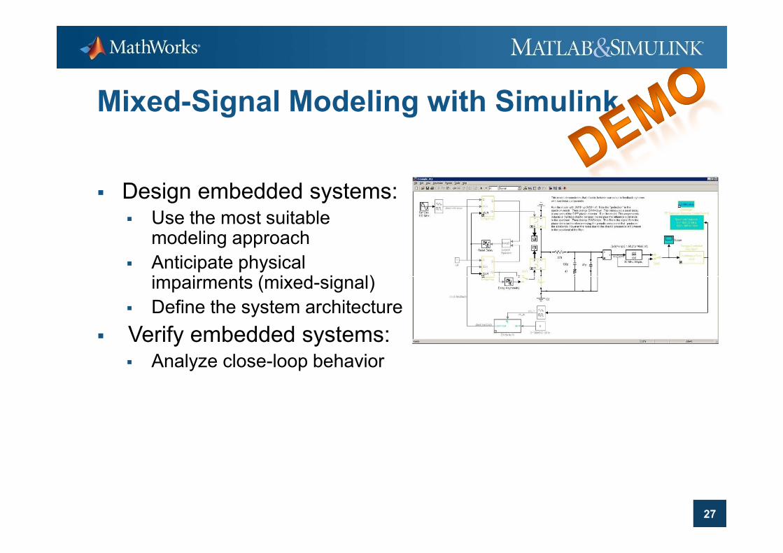
Mixed-Signal Modeling with Simulink
� Design embedded systems:� Use the most suitable
modeling approach
� Anticipate physical impairments (mixed-signal)
27
impairments (mixed-signal)
� Define the system architecture
� Verify embedded systems:� Analyze close-loop behavior
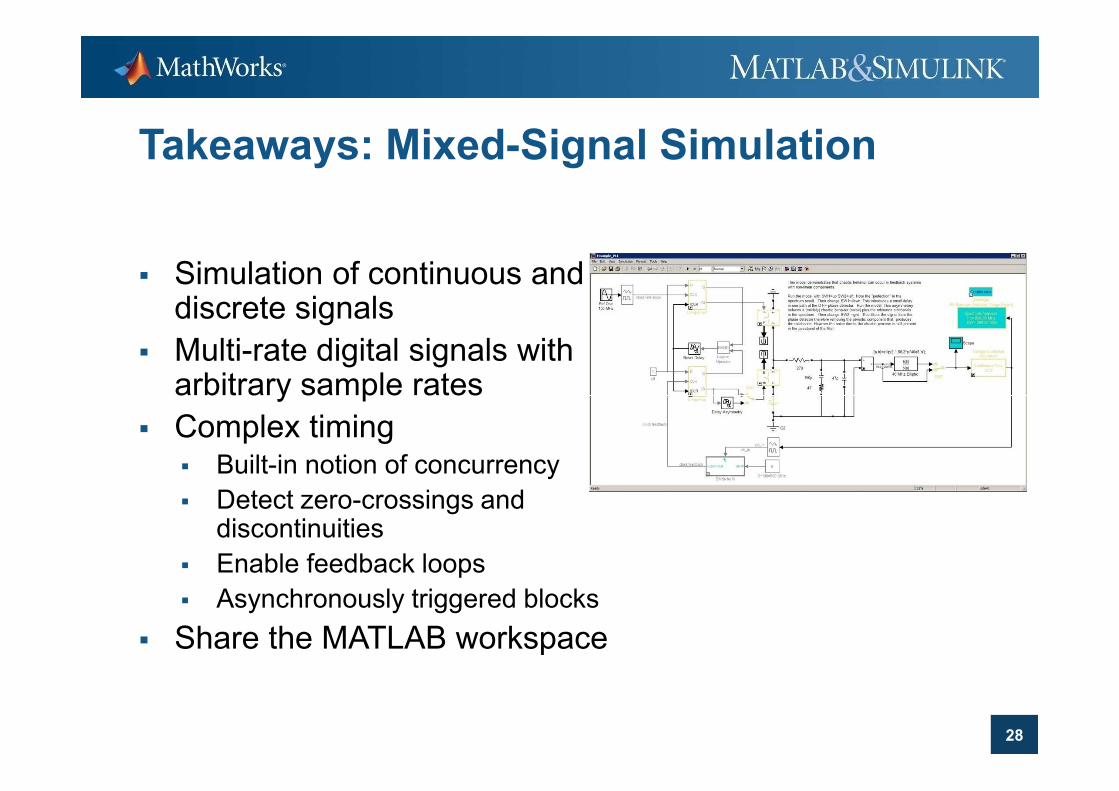
Takeaways: Mixed-Signal Simulation
� Simulation of continuous and discrete signals
� Multi-rate digital signals with arbitrary sample rates
28
arbitrary sample rates
� Complex timing� Built-in notion of concurrency
� Detect zero-crossings and discontinuities
� Enable feedback loops
� Asynchronously triggered blocks
� Share the MATLAB workspace
Challenges: RF System-Level Simulation
� Model RF front-ends:� Without being an expert
� With acceptable simulation speed
� Integrate baseband and RF simulation
29
� Integrate baseband and RF simulation� Develop a system-level view
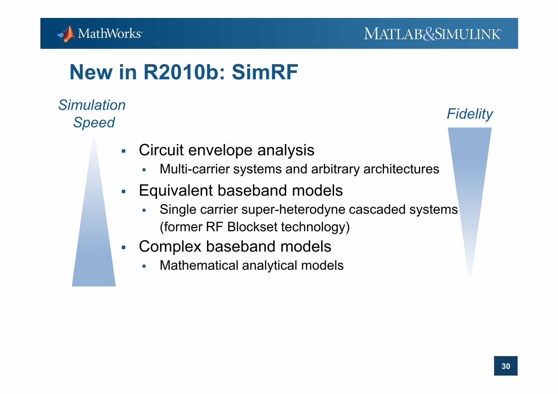
New in R2010b: SimRF
� Circuit envelope analysis� Multi-carrier systems and arbitrary architectures
� Equivalent baseband models
Simulation
SpeedFidelity
30
� Equivalent baseband models� Single carrier super-heterodyne cascaded systems
(former RF Blockset technology)
� Complex baseband models� Mathematical analytical models
Former RF Blockset TechnologySingle carrier simulation of cascaded RF systems
� Linear elements are modeled with baseband-complex
equivalent descriptions
� Nonlinear elements are described by means of (static)
AM/AM – AM/PM characteristics
31
AM/AM – AM/PM characteristics
� Elements are cascaded for fast single carrier simulations
in the time domain
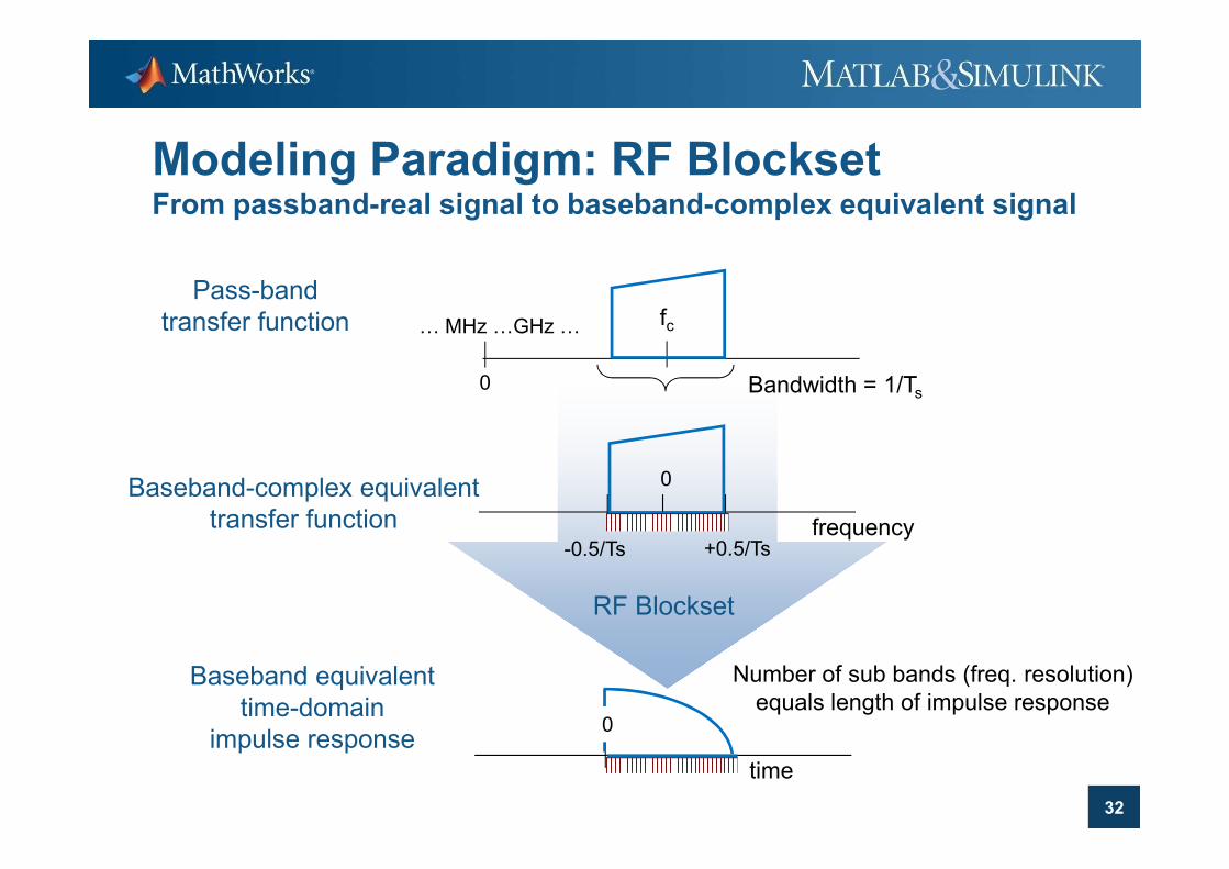
Modeling Paradigm: RF BlocksetFrom passband-real signal to baseband-complex equivalent signal
… MHz …GHz … fc
Bandwidth = 1/Ts0
Pass-band
transfer function
32
RF Blockset
0
-0.5/Ts +0.5/Ts
Baseband-complex equivalent
transfer function
Number of sub bands (freq. resolution)
equals length of impulse response
frequency
Baseband equivalent
time-domain
impulse responsetime
0
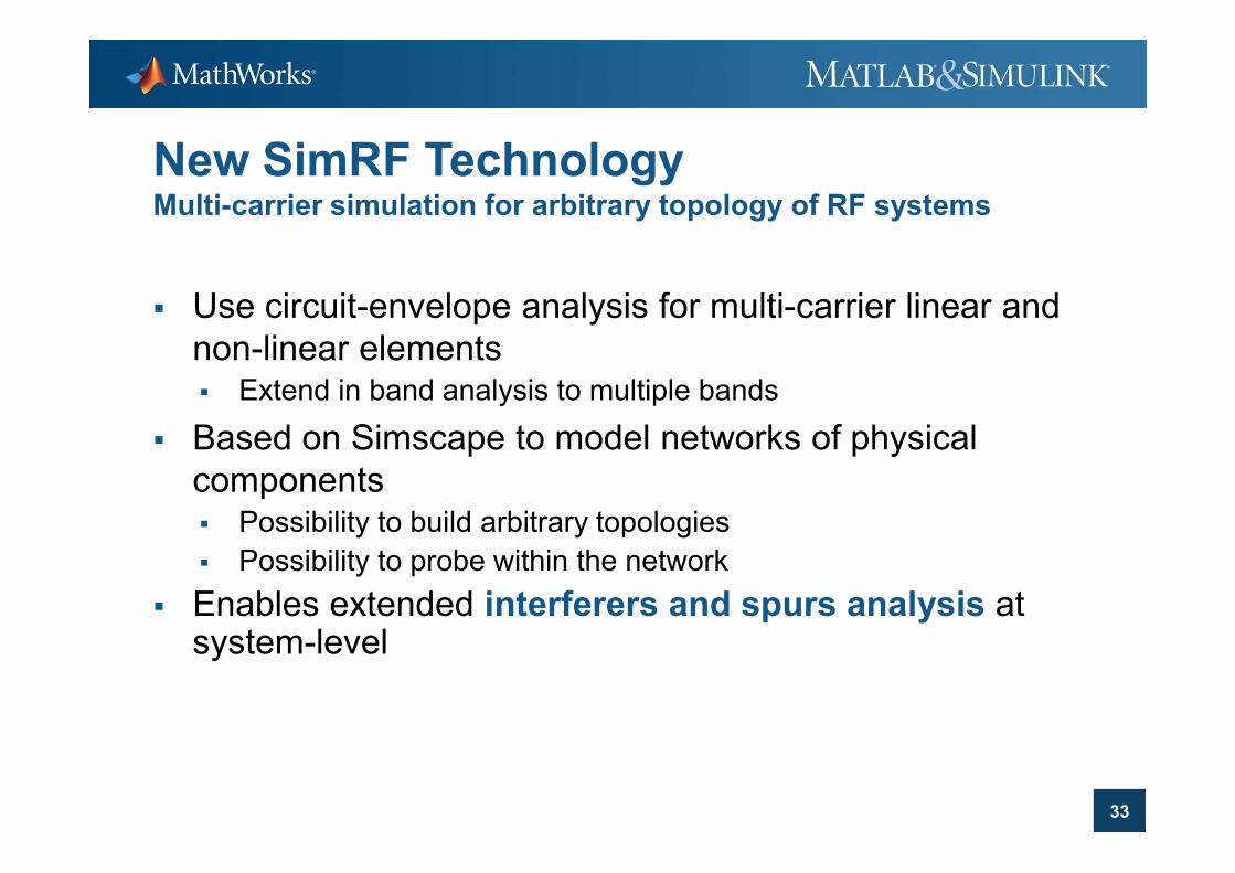
New SimRF TechnologyMulti-carrier simulation for arbitrary topology of RF systems
� Use circuit-envelope analysis for multi-carrier linear and
non-linear elements� Extend in band analysis to multiple bands
� Based on Simscape to model networks of physical
33
� Based on Simscape to model networks of physical
components� Possibility to build arbitrary topologies
� Possibility to probe within the network
� Enables extended interferers and spurs analysis at system-level
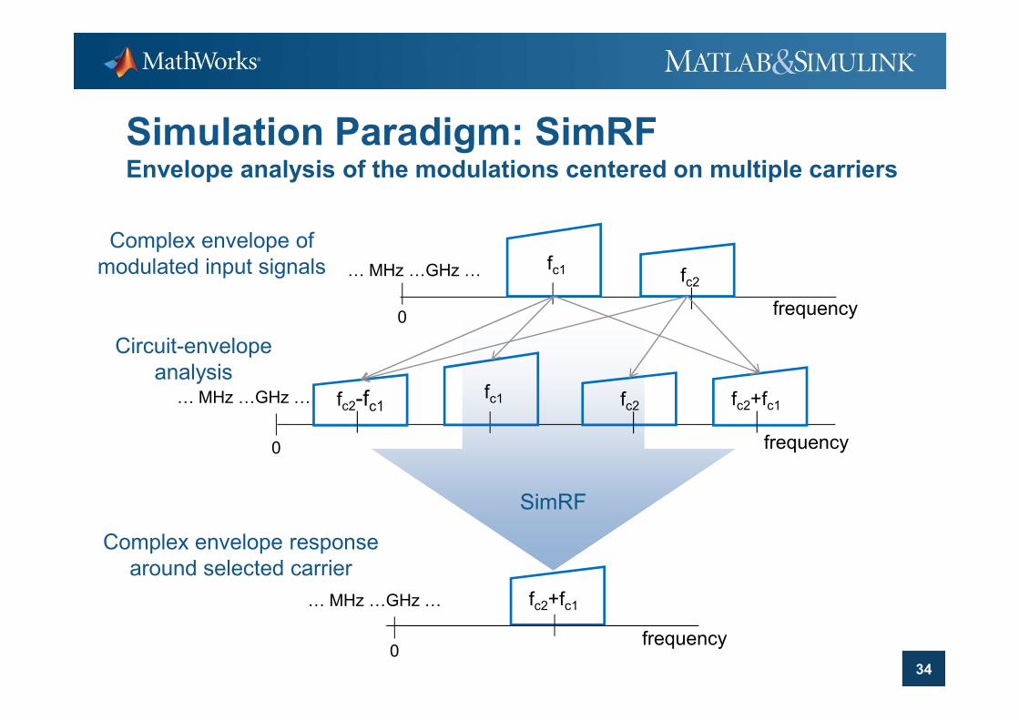
Simulation Paradigm: SimRFEnvelope analysis of the modulations centered on multiple carriers
… MHz …GHz … fc1
Circuit-envelope
analysis
0
Complex envelope of
modulated input signals fc2
frequency
34
SimRF
analysis
Complex envelope response
around selected carrier
… MHz …GHz …
0 frequency
fc1 fc2fc2-fc1 fc2+fc1
… MHz …GHz …
frequency
fc2+fc1
0
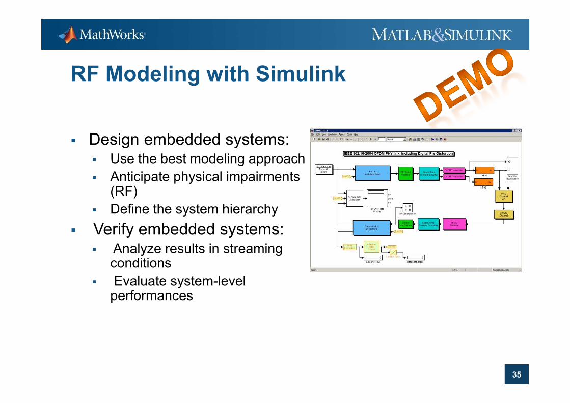
RF Modeling with Simulink
� Design embedded systems:� Use the best modeling approach
� Anticipate physical impairments (RF)
Define the system hierarchy
35
� Define the system hierarchy
� Verify embedded systems:� Analyze results in streaming
conditions
� Evaluate system-level performances
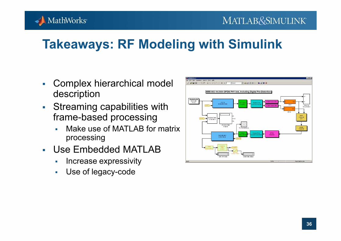
Takeaways: RF Modeling with Simulink
� Complex hierarchical model description
� Streaming capabilities with frame-based processing
36
frame-based processing� Make use of MATLAB for matrix
processing
� Use Embedded MATLAB � Increase expressivity
� Use of legacy-code
Design and Implement Signal Processing
Systems with MATLAB and Simulink
� Algorithm design
� Fast simulation
� Architecture exploration
� Targeting implementation
37
� Targeting implementation
� Verification and testing
� Rapid prototyping
Conclusions
� Quickly analyze and develop new algorithms with MATLAB
� Accurate system-level multi-domain analysis with Simulink
38
� Accurate system-level multi-domain analysis with Simulink
� With MATLAB and Simulink you can quickly design entire
systems with better performance