Signal Processing and its Applications...Signal Processing and its Applications addresses the entire breadth and depth of the subject with texts that cover the theory, technology and

Signal Processing and its Applications

SERIES EDITORS

Dr Richard GreenDepartment of Technology,Metropolitan Police Service,London, UK

Professor Truong NguyenDepartment of Electrical and ComputerEngineering,

Boston University, Boston, USA

EDITORIAL BOARD

Professor Maurice G. BellangerCNAM, Paris, France

Professor David BullDepartment of Electrical and ElectronicEngineering,University of Bristol, UK

Professor Gerry D. CainSchool of Electronic and ManufacturingSystem Engineering,University of Westminster, London, UK

Professor Colin CowanDepartment of Electronics and ElectricalEngineering,Queen’s University, Belfast, NorthernIreland

Professor Roy DaviesMachine Vision Group, Department ofPhysics,Royal Holloway, University of London,Surrey, UK

Dr Paola HobsonMotorola, Basingstoke, UK

Professor Mark SandlerDepartment of Electronics and ElectricalEngineering,King’s College London, University ofLondon, UK

Dr Henry StarkElectrical and Computer EngineeringDepartment,Illinois Institute of Technology, Chicago,USA

Dr Maneeshi Trivedi

Horndean, Waterlooville, UK

Books in the series

P. M. Clarkson and H. Stark, Signal Processing Methods for Audio, Images andTelecommunications (1995)

R. J. Clarke, Digital Compression of Still Images and Video (1995)

S-K. Chang and E. Jungert, Symbolic Projection for Image Information Retrievaland Spatial Reasoning (1996)

V. Cantoni, S. Levialdi and V. Roberto (eds.), Artificial Vision (1997)

R. de Mori, Spoken Dialogue with Computers (1998)

D. Bull, N. Canagarajah and A. Nix (eds.), Insights into Mobile MultimediaCommunications (1999)

A Handbook ofTime-Series Analysis,Signal Processingand Dynamics

D.S.G. POLLOCK

Queen Mary and Westfield CollegeThe University of LondonUK

ACADEMIC PRESS

San Diego • London • Boston • New YorkSydney • Tokyo • Toronto

This book is printed on acid-free paper.

Copyright c© 1999 by ACADEMIC PRESS

All Rights ReservedNo part of this publication may be reproduced or transmitted in any form or by any means electronicor mechanical, including photocopy, recording, or any information storage and retrieval system, withoutpermission in writing from the publisher.

Academic Press24–28 Oval Road, London NW1 7DX, UKhttp://www.hbuk.co.uk/ap/

Academic PressA Harcourt Science and Technology Company525 B Street, Suite 1900, San Diego, California 92101-4495, USAhttp://www.apnet.com

ISBN 0-12-560990-6

A catalogue record for this book is available from the British Library

Typeset by Focal Image Ltd, London, in collaboration with the author ΣπPrinted in Great Britain by The University Press, Cambridge

99 00 01 02 03 04 CU 9 8 7 6 5 4 3 2 1

Series Preface

Signal processing applications are now widespread. Relatively cheap consumerproducts through to the more expensive military and industrial systems extensivelyexploit this technology. This spread was initiated in the 1960s by the introduction ofcheap digital technology to implement signal processing algorithms in real-time forsome applications. Since that time semiconductor technology has developed rapidlyto support the spread. In parallel, an ever increasing body of mathematical theoryis being used to develop signal processing algorithms. The basic mathematicalfoundations, however, have been known and well understood for some time.

Signal Processing and its Applications addresses the entire breadth and depthof the subject with texts that cover the theory, technology and applications of signalprocessing in its widest sense. This is reflected in the composition of the EditorialBoard, who have interests in:

(i) Theory – The physics of the application and the mathematics to model thesystem;

(ii) Implementation – VLSI/ASIC design, computer architecture, numericalmethods, systems design methodology, and CAE;

(iii) Applications – Speech, sonar, radar, seismic, medical, communications (bothaudio and video), guidance, navigation, remote sensing, imaging, survey,archiving, non-destructive and non-intrusive testing, and personal entertain-ment.

Signal Processing and its Applications will typically be of most interest to post-graduate students, academics, and practising engineers who work in the field anddevelop signal processing applications. Some texts may also be of interest to finalyear undergraduates.

Richard C. GreenThe Engineering Practice,

Farnborough, UK

v

For Yasome Ranasinghe

Contents

Preface xxv

Introduction 1

1 The Methods of Time-Series Analysis 3The Frequency Domain and the Time Domain . . . . . . . . . . . . . . . 3Harmonic Analysis . . . . . . . . . . . . . . . . . . . . . . . . . . . . . . . 4Autoregressive and Moving-Average Models . . . . . . . . . . . . . . . . . 7Generalised Harmonic Analysis . . . . . . . . . . . . . . . . . . . . . . . . 10Smoothing the Periodogram . . . . . . . . . . . . . . . . . . . . . . . . . . 12The Equivalence of the Two Domains . . . . . . . . . . . . . . . . . . . . 12The Maturing of Time-Series Analysis . . . . . . . . . . . . . . . . . . . . 14Mathematical Appendix . . . . . . . . . . . . . . . . . . . . . . . . . . . . 16

Polynomial Methods 21

2 Elements of Polynomial Algebra 23Sequences . . . . . . . . . . . . . . . . . . . . . . . . . . . . . . . . . . . . 23Linear Convolution . . . . . . . . . . . . . . . . . . . . . . . . . . . . . . . 26Circular Convolution . . . . . . . . . . . . . . . . . . . . . . . . . . . . . . 28Time-Series Models . . . . . . . . . . . . . . . . . . . . . . . . . . . . . . . 30Transfer Functions . . . . . . . . . . . . . . . . . . . . . . . . . . . . . . . 31The Lag Operator . . . . . . . . . . . . . . . . . . . . . . . . . . . . . . . 33Algebraic Polynomials . . . . . . . . . . . . . . . . . . . . . . . . . . . . . 35Periodic Polynomials and Circular Convolution . . . . . . . . . . . . . . . 35Polynomial Factorisation . . . . . . . . . . . . . . . . . . . . . . . . . . . . 37Complex Roots . . . . . . . . . . . . . . . . . . . . . . . . . . . . . . . . . 38The Roots of Unity . . . . . . . . . . . . . . . . . . . . . . . . . . . . . . . 42The Polynomial of Degree n . . . . . . . . . . . . . . . . . . . . . . . . . . 43Matrices and Polynomial Algebra . . . . . . . . . . . . . . . . . . . . . . . 45Lower-Triangular Toeplitz Matrices . . . . . . . . . . . . . . . . . . . . . . 46Circulant Matrices . . . . . . . . . . . . . . . . . . . . . . . . . . . . . . . 48The Factorisation of Circulant Matrices . . . . . . . . . . . . . . . . . . . 50

3 Rational Functions and Complex Analysis 55Rational Functions . . . . . . . . . . . . . . . . . . . . . . . . . . . . . . . 55Euclid’s Algorithm . . . . . . . . . . . . . . . . . . . . . . . . . . . . . . . 55Partial Fractions . . . . . . . . . . . . . . . . . . . . . . . . . . . . . . . . 59The Expansion of a Rational Function . . . . . . . . . . . . . . . . . . . . 62Recurrence Relationships . . . . . . . . . . . . . . . . . . . . . . . . . . . 64Laurent Series . . . . . . . . . . . . . . . . . . . . . . . . . . . . . . . . . . 67

vii

D.S.G. POLLOCK: TIME-SERIES ANALYSIS

Analytic Functions . . . . . . . . . . . . . . . . . . . . . . . . . . . . . . . 70Complex Line Integrals . . . . . . . . . . . . . . . . . . . . . . . . . . . . 72The Cauchy Integral Theorem . . . . . . . . . . . . . . . . . . . . . . . . . 74Multiply Connected Domains . . . . . . . . . . . . . . . . . . . . . . . . . 76Integrals and Derivatives of Analytic Functions . . . . . . . . . . . . . . . 77Series Expansions . . . . . . . . . . . . . . . . . . . . . . . . . . . . . . . . 78Residues . . . . . . . . . . . . . . . . . . . . . . . . . . . . . . . . . . . . . 82The Autocovariance Generating Function . . . . . . . . . . . . . . . . . . 84The Argument Principle . . . . . . . . . . . . . . . . . . . . . . . . . . . . 86

4 Polynomial Computations 89Polynomials and their Derivatives . . . . . . . . . . . . . . . . . . . . . . . 90The Division Algorithm . . . . . . . . . . . . . . . . . . . . . . . . . . . . 94Roots of Polynomials . . . . . . . . . . . . . . . . . . . . . . . . . . . . . . 98Real Roots . . . . . . . . . . . . . . . . . . . . . . . . . . . . . . . . . . . 99Complex Roots . . . . . . . . . . . . . . . . . . . . . . . . . . . . . . . . . 104Muller’s Method . . . . . . . . . . . . . . . . . . . . . . . . . . . . . . . . 109Polynomial Interpolation . . . . . . . . . . . . . . . . . . . . . . . . . . . . 114Lagrangean Interpolation . . . . . . . . . . . . . . . . . . . . . . . . . . . 115Divided Differences . . . . . . . . . . . . . . . . . . . . . . . . . . . . . . . 117

5 Difference Equations and Differential Equations 121Linear Difference Equations . . . . . . . . . . . . . . . . . . . . . . . . . . 122Solution of the Homogeneous Difference Equation . . . . . . . . . . . . . . 123Complex Roots . . . . . . . . . . . . . . . . . . . . . . . . . . . . . . . . . 124Particular Solutions . . . . . . . . . . . . . . . . . . . . . . . . . . . . . . 126Solutions of Difference Equations with Initial Conditions . . . . . . . . . . 129Alternative Forms for the Difference Equation . . . . . . . . . . . . . . . . 133Linear Differential Equations . . . . . . . . . . . . . . . . . . . . . . . . . 135Solution of the Homogeneous Differential Equation . . . . . . . . . . . . . 136Differential Equation with Complex Roots . . . . . . . . . . . . . . . . . . 137Particular Solutions for Differential Equations . . . . . . . . . . . . . . . . 139Solutions of Differential Equations with Initial Conditions . . . . . . . . . 144Difference and Differential Equations Compared . . . . . . . . . . . . . . 147Conditions for the Stability of Differential Equations . . . . . . . . . . . . 148Conditions for the Stability of Difference Equations . . . . . . . . . . . . . 151

6 Vector Difference Equations and State-Space Models 161The State-Space Equations . . . . . . . . . . . . . . . . . . . . . . . . . . 161Conversions of Difference Equations to State-Space Form . . . . . . . . . 163Controllable Canonical State-Space Representations . . . . . . . . . . . . 165Observable Canonical Forms . . . . . . . . . . . . . . . . . . . . . . . . . 168Reduction of State-Space Equations to a Transfer Function . . . . . . . . 170Controllability . . . . . . . . . . . . . . . . . . . . . . . . . . . . . . . . . 171Observability . . . . . . . . . . . . . . . . . . . . . . . . . . . . . . . . . . 176

viii

CONTENTS

Least-Squares Methods 179

7 Matrix Computations 181Solving Linear Equations by Gaussian Elimination . . . . . . . . . . . . . 182Inverting Matrices by Gaussian Elimination . . . . . . . . . . . . . . . . . 188The Direct Factorisation of a Nonsingular Matrix . . . . . . . . . . . . . . 189The Cholesky Decomposition . . . . . . . . . . . . . . . . . . . . . . . . . 191Householder Transformations . . . . . . . . . . . . . . . . . . . . . . . . . 195The Q–R Decomposition of a Matrix of Full Column Rank . . . . . . . . 196

8 Classical Regression Analysis 201The Linear Regression Model . . . . . . . . . . . . . . . . . . . . . . . . . 201The Decomposition of the Sum of Squares . . . . . . . . . . . . . . . . . . 202Some Statistical Properties of the Estimator . . . . . . . . . . . . . . . . . 204Estimating the Variance of the Disturbance . . . . . . . . . . . . . . . . . 205The Partitioned Regression Model . . . . . . . . . . . . . . . . . . . . . . 206Some Matrix Identities . . . . . . . . . . . . . . . . . . . . . . . . . . . . . 206Computing a Regression via Gaussian Elimination . . . . . . . . . . . . . 208Calculating the Corrected Sum of Squares . . . . . . . . . . . . . . . . . . 211Computing the Regression Parameters via the Q–R Decomposition . . . . 215The Normal Distribution and the Sampling Distributions . . . . . . . . . 218Hypothesis Concerning the Complete Set of Coefficients . . . . . . . . . . 219Hypotheses Concerning a Subset of the Coefficients . . . . . . . . . . . . . 221An Alternative Formulation of the F statistic . . . . . . . . . . . . . . . . 223

9 Recursive Least-Squares Estimation 227Recursive Least-Squares Regression . . . . . . . . . . . . . . . . . . . . . . 227The Matrix Inversion Lemma . . . . . . . . . . . . . . . . . . . . . . . . . 228Prediction Errors and Recursive Residuals . . . . . . . . . . . . . . . . . . 229The Updating Algorithm for Recursive Least Squares . . . . . . . . . . . 231Initiating the Recursion . . . . . . . . . . . . . . . . . . . . . . . . . . . . 235Estimators with Limited Memories . . . . . . . . . . . . . . . . . . . . . . 236The Kalman Filter . . . . . . . . . . . . . . . . . . . . . . . . . . . . . . . 239Filtering . . . . . . . . . . . . . . . . . . . . . . . . . . . . . . . . . . . . . 241A Summary of the Kalman Equations . . . . . . . . . . . . . . . . . . . . 244An Alternative Derivation of the Kalman Filter . . . . . . . . . . . . . . . 245Smoothing . . . . . . . . . . . . . . . . . . . . . . . . . . . . . . . . . . . . 247Innovations and the Information Set . . . . . . . . . . . . . . . . . . . . . 247Conditional Expectations and Dispersions of the State Vector . . . . . . . 249The Classical Smoothing Algorithms . . . . . . . . . . . . . . . . . . . . . 250Variants of the Classical Algorithms . . . . . . . . . . . . . . . . . . . . . 254Multi-step Prediction . . . . . . . . . . . . . . . . . . . . . . . . . . . . . . 257

ix


10 Estimation of Polynomial Trends 261Polynomial Regression . . . . . . . . . . . . . . . . . . . . . . . . . . . . . 261The Gram–Schmidt Orthogonalisation Procedure . . . . . . . . . . . . . . 263A Modified Gram–Schmidt Procedure . . . . . . . . . . . . . . . . . . . . 266Uniqueness of the Gram Polynomials . . . . . . . . . . . . . . . . . . . . . 268Recursive Generation of the Polynomials . . . . . . . . . . . . . . . . . . . 270The Polynomial Regression Procedure . . . . . . . . . . . . . . . . . . . . 272Grafted Polynomials . . . . . . . . . . . . . . . . . . . . . . . . . . . . . . 278B-Splines . . . . . . . . . . . . . . . . . . . . . . . . . . . . . . . . . . . . 281Recursive Generation of B-spline Ordinates . . . . . . . . . . . . . . . . . 284Regression with B-Splines . . . . . . . . . . . . . . . . . . . . . . . . . . . 290

11 Smoothing with Cubic Splines 293Cubic Spline Interpolation . . . . . . . . . . . . . . . . . . . . . . . . . . . 294Cubic Splines and Bezier Curves . . . . . . . . . . . . . . . . . . . . . . . 301The Minimum-Norm Property of Splines . . . . . . . . . . . . . . . . . . . 305Smoothing Splines . . . . . . . . . . . . . . . . . . . . . . . . . . . . . . . 307A Stochastic Model for the Smoothing Spline . . . . . . . . . . . . . . . . 313Appendix: The Wiener Process and the IMA Process . . . . . . . . . . . 319

12 Unconstrained Optimisation 323Conditions of Optimality . . . . . . . . . . . . . . . . . . . . . . . . . . . 323Univariate Search . . . . . . . . . . . . . . . . . . . . . . . . . . . . . . . . 326Quadratic Interpolation . . . . . . . . . . . . . . . . . . . . . . . . . . . . 328Bracketing the Minimum . . . . . . . . . . . . . . . . . . . . . . . . . . . 335Unconstrained Optimisation via Quadratic Approximations . . . . . . . . 338The Method of Steepest Descent . . . . . . . . . . . . . . . . . . . . . . . 339The Newton–Raphson Method . . . . . . . . . . . . . . . . . . . . . . . . 340A Modified Newton Procedure . . . . . . . . . . . . . . . . . . . . . . . . 341The Minimisation of a Sum of Squares . . . . . . . . . . . . . . . . . . . . 343Quadratic Convergence . . . . . . . . . . . . . . . . . . . . . . . . . . . . 344The Conjugate Gradient Method . . . . . . . . . . . . . . . . . . . . . . . 347Numerical Approximations to the Gradient . . . . . . . . . . . . . . . . . 351Quasi-Newton Methods . . . . . . . . . . . . . . . . . . . . . . . . . . . . 352Rank-Two Updating of the Hessian Matrix . . . . . . . . . . . . . . . . . 354

Fourier Methods 363

13 Fourier Series and Fourier Integrals 365Fourier Series . . . . . . . . . . . . . . . . . . . . . . . . . . . . . . . . . . 367Convolution . . . . . . . . . . . . . . . . . . . . . . . . . . . . . . . . . . . 371Fourier Approximations . . . . . . . . . . . . . . . . . . . . . . . . . . . . 374Discrete-Time Fourier Transform . . . . . . . . . . . . . . . . . . . . . . . 377Symmetry Properties of the Fourier Transform . . . . . . . . . . . . . . . 378The Frequency Response of a Discrete-Time System . . . . . . . . . . . . 380The Fourier Integral . . . . . . . . . . . . . . . . . . . . . . . . . . . . . . 384

x

CONTENTS

The Uncertainty Relationship . . . . . . . . . . . . . . . . . . . . . . . . . 386The Delta Function . . . . . . . . . . . . . . . . . . . . . . . . . . . . . . 388Impulse Trains . . . . . . . . . . . . . . . . . . . . . . . . . . . . . . . . . 391The Sampling Theorem . . . . . . . . . . . . . . . . . . . . . . . . . . . . 392The Frequency Response of a Continuous-Time System . . . . . . . . . . 394Appendix of Trigonometry . . . . . . . . . . . . . . . . . . . . . . . . . . . 396Orthogonality Conditions . . . . . . . . . . . . . . . . . . . . . . . . . . . 397

14 The Discrete Fourier Transform 399Trigonometrical Representation of the DFT . . . . . . . . . . . . . . . . . 400Determination of the Fourier Coefficients . . . . . . . . . . . . . . . . . . 403The Periodogram and Hidden Periodicities . . . . . . . . . . . . . . . . . 405The Periodogram and the Empirical Autocovariances . . . . . . . . . . . . 408The Exponential Form of the Fourier Transform . . . . . . . . . . . . . . 410Leakage from Nonharmonic Frequencies . . . . . . . . . . . . . . . . . . . 413The Fourier Transform and the z-Transform . . . . . . . . . . . . . . . . . 414The Classes of Fourier Transforms . . . . . . . . . . . . . . . . . . . . . . 416Sampling in the Time Domain . . . . . . . . . . . . . . . . . . . . . . . . 418Truncation in the Time Domain . . . . . . . . . . . . . . . . . . . . . . . 421Sampling in the Frequency Domain . . . . . . . . . . . . . . . . . . . . . . 422Appendix: Harmonic Cycles . . . . . . . . . . . . . . . . . . . . . . . . . . 423

15 The Fast Fourier Transform 427Basic Concepts . . . . . . . . . . . . . . . . . . . . . . . . . . . . . . . . . 427The Two-Factor Case . . . . . . . . . . . . . . . . . . . . . . . . . . . . . 431The FFT for Arbitrary Factors . . . . . . . . . . . . . . . . . . . . . . . . 434Locating the Subsequences . . . . . . . . . . . . . . . . . . . . . . . . . . 437The Core of the Mixed-Radix Algorithm . . . . . . . . . . . . . . . . . . . 439Unscrambling . . . . . . . . . . . . . . . . . . . . . . . . . . . . . . . . . . 442The Shell of the Mixed-Radix Procedure . . . . . . . . . . . . . . . . . . . 445The Base-2 Fast Fourier Transform . . . . . . . . . . . . . . . . . . . . . . 447FFT Algorithms for Real Data . . . . . . . . . . . . . . . . . . . . . . . . 450FFT for a Single Real-valued Sequence . . . . . . . . . . . . . . . . . . . . 452

Time-Series Models 457

16 Linear Filters 459Frequency Response and Transfer Functions . . . . . . . . . . . . . . . . . 459Computing the Gain and Phase Functions . . . . . . . . . . . . . . . . . . 466The Poles and Zeros of the Filter . . . . . . . . . . . . . . . . . . . . . . . 469Inverse Filtering and Minimum-Phase Filters . . . . . . . . . . . . . . . . 475Linear-Phase Filters . . . . . . . . . . . . . . . . . . . . . . . . . . . . . . 477Locations of the Zeros of Linear-Phase Filters . . . . . . . . . . . . . . . . 479FIR Filter Design by Window Methods . . . . . . . . . . . . . . . . . . . 483Truncating the Filter . . . . . . . . . . . . . . . . . . . . . . . . . . . . . . 487Cosine Windows . . . . . . . . . . . . . . . . . . . . . . . . . . . . . . . . 492

xi


Design of Recursive IIR Filters . . . . . . . . . . . . . . . . . . . . . . . . 496IIR Design via Analogue Prototypes . . . . . . . . . . . . . . . . . . . . . 498The Butterworth Filter . . . . . . . . . . . . . . . . . . . . . . . . . . . . 499The Chebyshev Filter . . . . . . . . . . . . . . . . . . . . . . . . . . . . . 501The Bilinear Transformation . . . . . . . . . . . . . . . . . . . . . . . . . 504The Butterworth and Chebyshev Digital Filters . . . . . . . . . . . . . . . 506Frequency-Band Transformations . . . . . . . . . . . . . . . . . . . . . . . 507

17 Autoregressive and Moving-Average Processes 513Stationary Stochastic Processes . . . . . . . . . . . . . . . . . . . . . . . . 514Moving-Average Processes . . . . . . . . . . . . . . . . . . . . . . . . . . . 517Computing the MA Autocovariances . . . . . . . . . . . . . . . . . . . . . 521MA Processes with Common Autocovariances . . . . . . . . . . . . . . . . 522Computing the MA Parameters from the Autocovariances . . . . . . . . . 523Autoregressive Processes . . . . . . . . . . . . . . . . . . . . . . . . . . . . 528The Autocovariances and the Yule–Walker Equations . . . . . . . . . . . 528Computing the AR Parameters . . . . . . . . . . . . . . . . . . . . . . . . 535Autoregressive Moving-Average Processes . . . . . . . . . . . . . . . . . . 540Calculating the ARMA Parameters from the Autocovariances . . . . . . . 545

18 Time-Series Analysis in the Frequency Domain 549Stationarity . . . . . . . . . . . . . . . . . . . . . . . . . . . . . . . . . . . 550The Filtering of White Noise . . . . . . . . . . . . . . . . . . . . . . . . . 550Cyclical Processes . . . . . . . . . . . . . . . . . . . . . . . . . . . . . . . 553The Fourier Representation of a Sequence . . . . . . . . . . . . . . . . . . 555The Spectral Representation of a Stationary Process . . . . . . . . . . . . 556The Autocovariances and the Spectral Density Function . . . . . . . . . . 559The Theorem of Herglotz and the Decomposition of Wold . . . . . . . . . 561The Frequency-Domain Analysis of Filtering . . . . . . . . . . . . . . . . 564The Spectral Density Functions of ARMA Processes . . . . . . . . . . . . 566Canonical Factorisation of the Spectral Density Function . . . . . . . . . 570

19 Prediction and Signal Extraction 575Mean-Square Error . . . . . . . . . . . . . . . . . . . . . . . . . . . . . . . 576Predicting one Series from Another . . . . . . . . . . . . . . . . . . . . . . 577The Technique of Prewhitening . . . . . . . . . . . . . . . . . . . . . . . . 579Extrapolation of Univariate Series . . . . . . . . . . . . . . . . . . . . . . 580Forecasting with ARIMA Models . . . . . . . . . . . . . . . . . . . . . . . 583Generating the ARMA Forecasts Recursively . . . . . . . . . . . . . . . . 585Physical Analogies for the Forecast Function . . . . . . . . . . . . . . . . 587Interpolation and Signal Extraction . . . . . . . . . . . . . . . . . . . . . 589Extracting the Trend from a Nonstationary Sequence . . . . . . . . . . . . 591Finite-Sample Predictions: Hilbert Space Terminology . . . . . . . . . . . 593Recursive Prediction: The Durbin–Levinson Algorithm . . . . . . . . . . . 594A Lattice Structure for the Prediction Errors . . . . . . . . . . . . . . . . 599Recursive Prediction: The Gram–Schmidt Algorithm . . . . . . . . . . . . 601Signal Extraction from a Finite Sample . . . . . . . . . . . . . . . . . . . 607

xii

CONTENTS

Signal Extraction from a Finite Sample: the Stationary Case . . . . . . . 607Signal Extraction from a Finite Sample: the Nonstationary Case . . . . . 609

Time-Series Estimation 617

20 Estimation of the Mean and the Autocovariances 619Estimating the Mean of a Stationary Process . . . . . . . . . . . . . . . . 619Asymptotic Variance of the Sample Mean . . . . . . . . . . . . . . . . . . 621Estimating the Autocovariances of a Stationary Process . . . . . . . . . . 622Asymptotic Moments of the Sample Autocovariances . . . . . . . . . . . . 624Asymptotic Moments of the Sample Autocorrelations . . . . . . . . . . . . 626Calculation of the Autocovariances . . . . . . . . . . . . . . . . . . . . . . 629Inefficient Estimation of the MA Autocovariances . . . . . . . . . . . . . . 632Efficient Estimates of the MA Autocorrelations . . . . . . . . . . . . . . . 634

21 Least-Squares Methods of ARMA Estimation 637Representations of the ARMA Equations . . . . . . . . . . . . . . . . . . 637The Least-Squares Criterion Function . . . . . . . . . . . . . . . . . . . . 639The Yule–Walker Estimates . . . . . . . . . . . . . . . . . . . . . . . . . . 641Estimation of MA Models . . . . . . . . . . . . . . . . . . . . . . . . . . . 642Representations via LT Toeplitz Matrices . . . . . . . . . . . . . . . . . . 643Representations via Circulant Matrices . . . . . . . . . . . . . . . . . . . . 645The Gauss–Newton Estimation of the ARMA Parameters . . . . . . . . . 648An Implementation of the Gauss–Newton Procedure . . . . . . . . . . . . 649Asymptotic Properties of the Least-Squares Estimates . . . . . . . . . . . 655The Sampling Properties of the Estimators . . . . . . . . . . . . . . . . . 657The Burg Estimator . . . . . . . . . . . . . . . . . . . . . . . . . . . . . . 660

22 Maximum-Likelihood Methods of ARMA Estimation 667Matrix Representations of Autoregressive Models . . . . . . . . . . . . . . 667The AR Dispersion Matrix and its Inverse . . . . . . . . . . . . . . . . . . 669Density Functions of the AR Model . . . . . . . . . . . . . . . . . . . . . 672The Exact M-L Estimator of an AR Model . . . . . . . . . . . . . . . . . 673Conditional M-L Estimates of an AR Model . . . . . . . . . . . . . . . . . 676Matrix Representations of Moving-Average Models . . . . . . . . . . . . . 678The MA Dispersion Matrix and its Determinant . . . . . . . . . . . . . . 679Density Functions of the MA Model . . . . . . . . . . . . . . . . . . . . . 680The Exact M-L Estimator of an MA Model . . . . . . . . . . . . . . . . . 681Conditional M-L Estimates of an MA Model . . . . . . . . . . . . . . . . 685Matrix Representations of ARMA models . . . . . . . . . . . . . . . . . . 686Density Functions of the ARMA Model . . . . . . . . . . . . . . . . . . . 687Exact M-L Estimator of an ARMA Model . . . . . . . . . . . . . . . . . . 688

xiii


23 Nonparametric Estimation of the Spectral Density Function 697The Spectrum and the Periodogram . . . . . . . . . . . . . . . . . . . . . 698The Expected Value of the Sample Spectrum . . . . . . . . . . . . . . . . 702Asymptotic Distribution of The Periodogram . . . . . . . . . . . . . . . . 705Smoothing the Periodogram . . . . . . . . . . . . . . . . . . . . . . . . . . 710Weighting the Autocovariance Function . . . . . . . . . . . . . . . . . . . 713Weights and Kernel Functions . . . . . . . . . . . . . . . . . . . . . . . . . 714

Statistical Appendix: on Disc 721

24 Statistical Distributions 723Multivariate Density Functions . . . . . . . . . . . . . . . . . . . . . . . . 723Functions of Random Vectors . . . . . . . . . . . . . . . . . . . . . . . . . 725Expectations . . . . . . . . . . . . . . . . . . . . . . . . . . . . . . . . . . 726Moments of a Multivariate Distribution . . . . . . . . . . . . . . . . . . . 727Degenerate Random Vectors . . . . . . . . . . . . . . . . . . . . . . . . . . 729The Multivariate Normal Distribution . . . . . . . . . . . . . . . . . . . . 730Distributions Associated with the Normal Distribution . . . . . . . . . . . 733Quadratic Functions of Normal Vectors . . . . . . . . . . . . . . . . . . . 734The Decomposition of a Chi-square Variate . . . . . . . . . . . . . . . . . 736Limit Theorems . . . . . . . . . . . . . . . . . . . . . . . . . . . . . . . . . 739Stochastic Convergence . . . . . . . . . . . . . . . . . . . . . . . . . . . . 740The Law of Large Numbers and the Central Limit Theorem . . . . . . . . 745

25 The Theory of Estimation 749Principles of Estimation . . . . . . . . . . . . . . . . . . . . . . . . . . . . 749Identifiability . . . . . . . . . . . . . . . . . . . . . . . . . . . . . . . . . . 750The Information Matrix . . . . . . . . . . . . . . . . . . . . . . . . . . . . 753The Efficiency of Estimation . . . . . . . . . . . . . . . . . . . . . . . . . 754Unrestricted Maximum-Likelihood Estimation . . . . . . . . . . . . . . . . 756Restricted Maximum-Likelihood Estimation . . . . . . . . . . . . . . . . . 758Tests of the Restrictions . . . . . . . . . . . . . . . . . . . . . . . . . . . . 761

xiv

PROGRAMS: Listed by Chapter

TEMPORAL SEQUENCES AND POLYNOMIAL ALGEBRA

(2.14) procedure Convolution(var alpha, beta : vector;p, k : integer);

(2.19) procedure Circonvolve(alpha, beta : vector;var gamma : vector;n : integer);

(2.50) procedure QuadraticRoots(a, b, c : real);

(2.59) function Cmod(a : complex) : real;

(2.61) function Cadd(a, b : complex) : complex;

(2.65) function Cmultiply(a, b : complex) : complex;

(2.67) function Cinverse(a : complex) : complex;

(2.68) function Csqrt(a : complex) : complex;

(2.76) procedure RootsToCoefficients(n : integer;var alpha, lambda : complexVector);

(2.79) procedure InverseRootsToCoeffs(n : integer;var alpha,mu : complexVector);

RATIONAL FUNCTIONS AND COMPLEX ANALYSIS

(3.43) procedure RationalExpansion(alpha : vector;p, k, n : integer;var beta : vector);

(3.46) procedure RationalInference(omega : vector;p, k : integer;var beta, alpha : vector);

(3.49) procedure BiConvolution(var omega, theta,mu : vector;p, q, g, h : integer);

POLYNOMIAL COMPUTATIONS

(4.11) procedure Horner(alpha : vector;

xv


p : integer;xi : real;var gamma0 : real;var beta : vector);

(4.16) procedure ShiftedForm(var alpha : vector;xi : real;p : integer);

(4.17) procedure ComplexPoly(alpha : complexVector;p : integer;z : complex;var gamma0 : complex;var beta : complexVector);

(4.46) procedure DivisionAlgorithm(alpha, delta : vector;p, q : integer;var beta : jvector;var rho : vector);

(4.52) procedure RealRoot(p : integer;alpha : vector;var root : real;var beta : vector);

(4.53) procedure NRealRoots(p, nOfRoots : integer;var alpha, beta, lambda : vector);

(4.68) procedure QuadraticDeflation(alpha : vector;delta0, delta1 : real;p : integer;var beta : vector;var c0, c1, c2 : real);

(4.70) procedure Bairstow(alpha : vector;p : integer;var delta0, delta1 : real;var beta : vector);

(4.72) procedure MultiBairstow(p : integer;var alpha : vector;var lambda : complexVector);

(4.73) procedure RootsOfFactor(i : integer;delta0, delta1 : real;var lambda : complexVector);

xvi


(4.78) procedure Mueller(p : integer;poly : complexVector;var root : complex;var quotient : complexVector);

(4.79) procedure ComplexRoots(p : integer;var alpha, lambda : complexVector);

DIFFERENTIAL AND DIFFERENCE EQUATIONS

(5.137) procedure RouthCriterion(phi : vector;p : integer;var stable : boolean);

(5.161) procedure JuryCriterion(alpha : vector;p : integer;var stable : boolean);

MATRIX COMPUTATIONS

(7.28) procedure LUsolve(start, n : integer;var a : matrix;var x, b : vector);

(7.29) procedure GaussianInversion(n, stop : integer;var a : matrix);

(7.44) procedure Cholesky(n : integer;var a : matrix;var x, b : vector);

(7.47) procedure LDLprimeDecomposition(n : integer;var a : matrix);

(7.63) procedure Householder(var a, b : matrix;m,n, q : integer);

CLASSICAL REGRESSION ANALYSIS

(8.54) procedure Correlation(n, Tcap : integer;var x, c : matrix;var scale,mean : vector);

xvii


(8.56) procedure GaussianRegression(k, Tcap : integer;var x, c : matrix);

(8.70) procedure QRregression(Tcap, k : integer;var x, y, beta : matrix;var varEpsilon : real);

(8.71) procedure Backsolve(var r, x, b : matrix;n, q : integer);

RECURSIVE LEAST-SQUARES METHODS

(9.26) procedure RLSUpdate(x : vector;k, sign : integer;y, lambda : real;var h : real;var beta, kappa : vector;var p : matrix);

(9.34) procedure SqrtUpdate(x : vector;k : integer;y, lambda : real;var h : real;var beta, kappa : vector;var s : matrix);

POLYNOMIAL TREND ESTIMATION

(10.26) procedure GramSchmidt(var phi, r : matrix;n, q : integer);

(10.50) procedure PolyRegress(x, y : vector;var alpha, gamma, delta, poly : vector;q, n : integer);

(10.52) procedure OrthoToPower(alpha, gamma, delta : vector;var beta : vector;q : integer);

(10.62) function PolyOrdinate(x : real;alpha, gamma, delta : vector;q : integer) : real;

xviii


(10.100) procedure BSplineOrdinates(p : integer;x : real;xi : vector;var b : vector);

(10.101) procedure BSplineCoefficients(p : integer;xi : vector;mode : string;var c : matrix);

SPLINE SMOOTHING

(11.18) procedure CubicSplines(var S : SplineVec;n : integer);

(11.50) procedure SplinetoBezier(S : SplineVec;var B : BezierVec;n : integer);

(11.83) procedure Quincunx(n : integer;var u, v, w, q : vector);

(11.84) procedure SmoothingSpline(var S : SplineVec;sigma : vector;lambda : real;n : integer);

NONLINEAR OPTIMISATION

(12.13) procedure GoldenSearch(function Funct(x : real) : real;var a, b : real;limit : integer;tolerance : real);

(12.20) procedure Quadratic(var p, q : real;a, b, c, fa, fb, fc : real);

(12.22) procedure QuadraticSearch(function Funct(lambda : real;theta, pvec : vector;n : integer) : real;

var a, b, c, fa, fb, fc : real;theta, pvec : vector;n : integer);

xix


(12.26) function Check(mode : string;a, b, c, fa, fb, fc, fw : real) : boolean;

(12.27) procedure LineSearch(function Funct(lambda : real;theta, pvec : vector;n : integer) : real;

var a : real;theta, pvec : vector;n : integer);

(12.82) procedure ConjugateGradients(function Funct(lambda : real;theta, pvec : vector;n : integer) : real;

var theta : vector;n : integer);

(12.87) procedure fdGradient(function Funct(lambda : real;theta, pvec : vector;n : integer) : real;

var gamma : vector;theta : vector;n : integer);

(12.119) procedure BFGS(function Funct(lambda : real;theta, pvec : vector;n : integer) : real;

var theta : vector;n : integer);

THE FAST FOURIER TRANSFORM

(15.8) procedure PrimeFactors(Tcap : integer;var g : integer;var N : ivector;var palindrome : boolean);

(15.45) procedure MixedRadixCore(var yReal, yImag : vector;var N,P,Q : ivector;Tcap, g : integer);

(15.49) function tOfj(j, g : integer;P,Q : ivector) : integer;

(15.50) procedure ReOrder(P,Q : ivector;Tcap, g : integer;var yImag, yReal : vector);

xx


(15.51) procedure MixedRadixFFT(var yReal, yImag : vector;var Tcap, g : integer;inverse : boolean);

(15.54) procedure Base2FFT(var y : longVector;Tcap, g : integer);

(15.63) procedure TwoRealFFTs(var f, d : longVectorTcap, g : integer);

(15.74) procedure OddSort(Ncap : integer;var y : longVector);

(15.77) procedure CompactRealFFT(var x : longVector;Ncap, g : integer);

LINEAR FILTERING

(16.20) procedure GainAndPhase(var gain, phase : real;delta, gamma : vector;omega : real;d, g : integer);

(16.21) function Arg(psi : complex) : real;

LINEAR TIME-SERIES MODELS

(17.24) procedure MACovariances(var mu, gamma : vector;var varEpsilon : real;q : integer);

(17.35) procedure MAParameters(var mu : vector;var varEpsilon : real;

gamma : vector;q : integer);

(17.39) procedure Minit(var mu : vector;var varEpsilon : real;gamma : vector;q : integer);

(17.40) function CheckDelta(tolerance : real;q : integer;

xxi


var delta,mu : vector) : boolean;

(17.67) procedure YuleWalker(p, q : integer;gamma : vector;var alpha : vector;var varEpsilon : real);

(17.75) procedure LevinsonDurbin(gamma : vector;p : integer;var alpha, pacv : vector);

(17.98) procedure ARMACovariances(alpha,mu : vector;var gamma : vector;var varEpsilon : real;lags, p, q : integer);

(17.106) procedure ARMAParameters(p, q : integer;gamma : vector;var alpha,mu : vector;var varEpsilon : real);

PREDICTION

(19.139) procedure GSPrediction(gamma : vector;y : longVector;var mu : matrix;n, q : integer);

ESTIMATION OF THE MEAN AND THE AUTOCOVARIANCES

(20.55) procedure Autocovariances(Tcap, lag : integer;var y : longVector;var acovar : vector);

(20.59) procedure FourierACV(var y : longVector;lag, Tcap : integer);

ARMA ESTIMATION: ASYMPTOTIC METHODS

(21.55) procedure Covariances(x, y : longVector;var covar : jvector;n, p, q : integer);

xxii


(21.57) procedure MomentMatrix(covarYY, covarXX, covarXY : jvector;p, q : integer;var moments : matrix);

(21.58) procedure RHSVector(moments : matrix;covarYY, covarXY : jvector;alpha : vector;p, q : integer;var rhVec : vector);

(21.59) procedure GaussNewtonARMA(p, q, n : integer;y : longVector;var alpha,mu : vector);

(21.87) procedure BurgEstimation(var alpha, pacv : vector;y : longVector;p, Tcap : integer);

ARMA ESTIMATION: MAXIMUM-LIKELIHOOD METHODS

(22.40) procedure ARLikelihood(var S, varEpsilon : real;var y : longVector;alpha : vector;Tcap, p : integer;var stable : boolean);

(22.74) procedure MALikelihood(var S, varEpsilon : real;var y : longVector;mu : vector;Tcap, q : integer);

(22.106) procedure ARMALikelihood(var S, varEpsilon : real;alpha,mu : vector;y : longVector;Tcap, p, q : integer);

xxiii

Preface

It is hoped that this book will serve both as a text in time-series analysis and signalprocessing and as a reference book for research workers and practitioners. Time-series analysis and signal processing are two subjects which ought to be treatedas one; and they are the concern of a wide range of applied disciplines includ-ing statistics, electrical engineering, mechanical engineering, physics, medicine andeconomics.

The book is primarily a didactic text and, as such, it has three main aspects.The first aspect of the exposition is the mathematical theory which is the foundationof the two subjects. The book does not skimp this. The exposition begins inChapters 2 and 3 with polynomial algebra and complex analysis, and it reachesinto the middle of the book where a lengthy chapter on Fourier analysis is to befound.

The second aspect of the exposition is an extensive treatment of the numericalanalysis which is specifically related to the subjects of time-series analysis andsignal processing but which is, usually, of a much wider applicability. This be-gins in earnest with the account of polynomial computation, in Chapter 4, andof matrix computation, in Chapter 7, and it continues unabated throughout thetext. The computer code, which is the product of the analysis, is distributedevenly throughout the book, but it is also hierarchically ordered in the sense thatcomputer procedures which come later often invoke their predecessors.

The third and most important didactic aspect of the text is the exposition ofthe subjects of time-series analysis and signal processing themselves. This beginsas soon as, in logic, it can. However, the fact that the treatment of the substantiveaspects of the subject is delayed until the mathematical foundations are in placeshould not prevent the reader from embarking immediately upon such topics as thestatistical analysis of time series or the theory of linear filtering. The book has beenassembled in the expectation that it will be read backwards as well as forwards, asis usual with such texts. Therefore it contains extensive cross-referencing.

The book is also intended as an accessible work of reference. The computercode which implements the algorithms is woven into the text so that it binds closelywith the mathematical exposition; and this should allow the detailed workings ofthe algorithms to be understood quickly. However, the function of each of the Pascalprocedures and the means of invoking them are described in a reference section,and the code of the procedures is available in electronic form on a computer disc.

The associated disc contains the Pascal code precisely as it is printed in thetext. An alternative code in the C language is also provided. Each procedure iscoupled with a so-called driver, which is a small program which shows the procedurein action. The essential object of the driver is to demonstrate the workings ofthe procedure; but usually it fulfils the additional purpose of demonstrating someaspect the theory which has been set forth in the chapter in which the code of theprocedure it to be found. It is hoped that, by using the algorithms provided in thisbook, scientists and engineers will be able to piece together reliable software toolstailored to their own specific needs.

xxv

Preface

The compact disc also contains a collection of reference material which includesthe libraries of the computer routines and various versions of the bibliography ofthe book. The numbers in brackets which accompany the bibliographic citationsrefer to their order in the composite bibliography which is to be found on the disc.On the disc, there is also a bibliography which is classified by subject area.

A preface is the appropriate place to describe the philosophy and the motiva-tion of the author in so far as they affect the book. A characteristic of this book,which may require some justification, is its heavy emphasis on the mathematicalfoundations of its subjects. There are some who regard mathematics as a burdenwhich should be eased or lightened whenever possible. The opinion which is re-flected in the book is that a firm mathematical framework is needed in order to bearthe weight of the practical subjects which are its principal concern. For example,it seems that, unless the reader is adequately appraised of the notions underlyingFourier analysis, then the perplexities and confusions which will inevitably arisewill limit their ability to commit much of the theory of linear filters to memory.Practical mathematical results which are well-supported by theory are far moreaccessible than those which are to be found beneath piles of technological detritus.

Another characteristic of the book which reflects a methodological opinion isthe manner in which the computer code is presented. There are some who regardcomputer procedures merely as technological artefacts to be encapsulated in boxeswhose contents are best left undisturbed for fear of disarranging them. An oppositeopinion is reflected in this book. The computer code presented here should be readand picked to pieces before being reassembled in whichever way pleases the reader.In short, the computer procedures should be approached in a spirit of constructiveplay. An individual who takes such an approach in general will not be balked bythe non-availability of a crucial procedure or by the incapacity of some large-scalecomputer program upon which they have come to rely. They will be preparedto make for themselves whatever tools they happen to need for their immediatepurposes.

The advent of the microcomputer has enabled the approach of individualistself-help advocated above to become a practical one. At the same time, it hasstimulated the production of a great variety of highly competent scientific softwarewhich is supplied commercially. It often seems like wasted effort to do for oneselfwhat can sometimes be done better by purpose-built commercial programs. Clearly,there are opposing forces at work here—and the issue is the perennial one of whetherwe are to be the masters or the slaves of our technology. The conflict will never beresolved; but a balance can be struck. This book, which aims to help the reader tomaster one of the central technologies of the latter half of this century, places mostof its weight on one side of the scales.

D.S.G. POLLOCK

xxvi

Introduction

CHAPTER 1

The Methods ofTime-Series Analysis

The methods to be presented in this book are designed for the purpose of analysingseries of statistical observations taken at regular intervals in time. The methodshave a wide range of applications. We can cite astronomy [539], meteorology [444],seismology [491], oceanography [232], [251], communications engineering and signalprocessing [425], the control of continuous process plants [479], neurology and elec-troencephalography [151], [540], and economics [233]; and this list is by no meanscomplete.

The Frequency Domain and the Time Domain

The methods apply, in the main, to what are described as stationary or non-evolutionary time series. Such series manifest statistical properties which are in-variant throughout time, so that the behaviour during one epoch is the same as itwould be during any other.

When we speak of a weakly stationary or covariance-stationary process, wehave in mind a sequence of random variables y(t) = {yt; t = 0,±1,±2, . . .}, rep-resenting the potential observations of the process, which have a common finiteexpected value E(yt) = µ and a set of autocovariances C(yt, ys) = E{(yt − µ)(ys −µ)} = γ|t−s| which depend only on the temporal separation τ = |t− s| of the datest and s and not on their absolute values. Usually, we require of such a processthat lim(τ → ∞)γτ = 0, which is to say that the correlation between increasinglyremote elements of the sequence tends to zero. This is a way of expressing thenotion that the events of the past have a diminishing effect upon the present asthey recede in time. In an appendix to the chapter, we review the definitions ofmathematical expectations and covariances.

There are two distinct yet broadly equivalent modes of time-series analysiswhich may be pursued. On the one hand are the time-domain methods whichhave their origin in the classical theory of correlation. Such methods deal pre-ponderantly with the autocovariance functions and the cross-covariance functionsof the series, and they lead inevitably towards the construction of structural orparametric models of the autoregressive moving-average type for single series andof the transfer-function type for two or more causally related series. Many of themethods which are used to estimate the parameters of these models can be viewedas sophisticated variants of the method of linear regression.

On the other hand are the frequency-domain methods of spectral analysis.These are based on an extension of the methods of Fourier analysis which originate

3


in the idea that, over a finite interval, any analytic function can be approximated,to whatever degree of accuracy is desired, by taking a weighted sum of sine andcosine functions of harmonically increasing frequencies.

Harmonic Analysis

The astronomers are usually given credit for being the first to apply the meth-ods of Fourier analysis to time series. Their endeavours could be described as thesearch for hidden periodicities within astronomical data. Typical examples werethe attempts to uncover periodicities within the activities recorded by the Wolfersunspot index—see Izenman [266]—and in the indices of luminosity of variablestars.

The relevant methods were developed over a long period of time. Lagrange[306] suggested methods for detecting hidden periodicities in 1772 and 1778. TheDutchman Buijs-Ballot [86] propounded effective computational procedures for thestatistical analysis of astronomical data in 1847. However, we should probablycredit Sir Arthur Schuster [444], who in 1889 propounded the technique of periodo-gram analysis, with being the progenitor of the modern methods for analysing timeseries in the frequency domain.

In essence, these frequency-domain methods envisaged a model underlying theobservations which takes the form of

y(t) =∑j

ρj cos(ωjt− θj) + ε(t)

=∑j

{αj cos(ωjt) + βj sin(ωjt)

}+ ε(t),

(1.1)

where αj = ρj cos θj and βj = ρj sin θj , and where ε(t) is a sequence of indepen-dently and identically distributed random variables which we call a white-noiseprocess. Thus the model depicts the series y(t) as a weighted sum of perfectlyregular periodic components upon which is superimposed a random component.

The factor ρj =√

(α2j + β2

j ) is called the amplitude of the jth periodic com-ponent, and it indicates the importance of that component within the sum. Sincethe variance of a cosine function, which is also called its mean-square deviation, isjust one half, and since cosine functions at different frequencies are uncorrelated,it follows that the variance of y(t) is expressible as V {y(t)} = 1

2

∑j ρ

2j + σ2

ε whereσ2ε = V {ε(t)} is the variance of the noise.

The periodogram is simply a device for determining how much of the varianceof y(t) is attributable to any given harmonic component. Its value at ωj = 2πj/T ,calculated from a sample y0, . . . , yT−1 comprising T observations on y(t), is givenby

I(ωj) =2T

[{∑t

yt cos(ωjt)}2

+{∑

t

yt sin(ωjt)}2]

=T

2{a2(ωj) + b2(ωj)

}.

(1.2)

4

1: THE METHODS OF TIME-SERIES ANALYSIS

0 10 20 30 40 50 60 70 80 90

Figure 1.1. The graph of a sine function.

0 10 20 30 40 50 60 70 80 90

Figure 1.2. Graph of a sine function with small random fluctuations superimposed.

If y(t) does indeed comprise only a finite number of well-defined harmonic compo-nents, then it can be shown that 2I(ωj)/T is a consistent estimator of ρ2

j in thesense that it converges to the latter in probability as the size T of the sample ofthe observations on y(t) increases.

The process by which the ordinates of the periodogram converge upon thesquared values of the harmonic amplitudes was well expressed by Yule [539] in aseminal article of 1927:

If we take a curve representing a simple harmonic function of time, andsuperpose on the ordinates small random errors, the only effect is to makethe graph somewhat irregular, leaving the suggestion of periodicity stillclear to the eye (see Figures 1.1 and 1.2). If the errors are increased inmagnitude, the graph becomes more irregular, the suggestion of periodic-ity more obscure, and we have only sufficiently to increase the errors tomask completely any appearance of periodicity. But, however large theerrors, periodogram analysis is applicable to such a curve, and, given asufficient number of periods, should yield a close approximation to theperiod and amplitude of the underlying harmonic function.

5


0

50

100

150

1750 1760 1770 1780 1790 1800 1810 1820 1830

0

50

100

150

1840 1850 1860 1870 1880 1890 1900 1910 1920

Figure 1.3. Wolfer’s sunspot numbers 1749–1924.

We should not quote this passage without mentioning that Yule proceeded toquestion whether the hypothesis underlying periodogram analysis, which postulatesthe equation under (1.1), was an appropriate hypothesis for all cases.

A highly successful application of periodogram analysis was that of Whittakerand Robinson [515] who, in 1924, showed that the series recording the brightness ormagnitude of the star T. Ursa Major over 600 days could be fitted almost exactly bythe sum of two harmonic functions with periods of 24 and 29 days. This led to thesuggestion that what was being observed was actually a two-star system wherein thelarger star periodically masked the smaller, brighter star. Somewhat less successfulwere the attempts of Arthur Schuster himself [445] in 1906 to substantiate the claimthat there is an 11-year cycle in the activity recorded by the Wolfer sunspot index(see Figure 1.3).

Other applications of the method of periodogram analysis were even less suc-cessful; and one application which was a significant failure was its use by WilliamBeveridge [51], [52] in 1921 and 1922 to analyse a long series of European wheatprices. The periodogram of this data had so many peaks that at least twentypossible hidden periodicities could be picked out, and this seemed to be manymore than could be accounted for by plausible explanations within the realm ofeconomic history. Such experiences seemed to point to the inappropriateness to

6


economic circumstances of a model containing perfectly regular cycles. A classicexpression of disbelief was made by Slutsky [468] in another article of 1927:

Suppose we are inclined to believe in the reality of the strict periodicity ofthe business cycle, such, for example, as the eight-year period postulatedby Moore [352]. Then we should encounter another difficulty. Whereinlies the source of this regularity? What is the mechanism of causalitywhich, decade after decade, reproduces the same sinusoidal wave whichrises and falls on the surface of the social ocean with the regularity of dayand night?

Autoregressive and Moving-Average Models

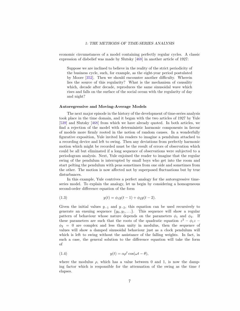
The next major episode in the history of the development of time-series analysistook place in the time domain, and it began with the two articles of 1927 by Yule[539] and Slutsky [468] from which we have already quoted. In both articles, wefind a rejection of the model with deterministic harmonic components in favourof models more firmly rooted in the notion of random causes. In a wonderfullyfigurative exposition, Yule invited his readers to imagine a pendulum attached toa recording device and left to swing. Then any deviations from perfectly harmonicmotion which might be recorded must be the result of errors of observation whichcould be all but eliminated if a long sequence of observations were subjected to aperiodogram analysis. Next, Yule enjoined the reader to imagine that the regularswing of the pendulum is interrupted by small boys who get into the room andstart pelting the pendulum with peas sometimes from one side and sometimes fromthe other. The motion is now affected not by superposed fluctuations but by truedisturbances.

In this example, Yule contrives a perfect analogy for the autoregressive time-series model. To explain the analogy, let us begin by considering a homogeneoussecond-order difference equation of the form

y(t) = φ1y(t− 1) + φ2y(t− 2).(1.3)

Given the initial values y−1 and y−2, this equation can be used recursively togenerate an ensuing sequence {y0, y1, . . .}. This sequence will show a regularpattern of behaviour whose nature depends on the parameters φ1 and φ2. Ifthese parameters are such that the roots of the quadratic equation z2 − φ1z −φ2 = 0 are complex and less than unity in modulus, then the sequence ofvalues will show a damped sinusoidal behaviour just as a clock pendulum willwhich is left to swing without the assistance of the falling weights. In fact, insuch a case, the general solution to the difference equation will take the formof

y(t) = αρt cos(ωt− θ),(1.4)

where the modulus ρ, which has a value between 0 and 1, is now the damp-ing factor which is responsible for the attenuation of the swing as the time telapses.

7


0 10 20 30 40 50 60 70 80 90

Figure 1.4. A series generated by Yule’s equationy(t) = 1.343y(t− 1)− 0.655y(t− 2) + ε(t).

0 10 20 30 40 50 60 70 80 90

Figure 1.5. A series generated by the equationy(t) = 1.576y(t− 1)− 0.903y(t− 2) + ε(t).

The autoregressive model which Yule was proposing takes the form of

y(t) = φ1y(t− 1) + φ2y(t− 2) + ε(t),(1.5)

where ε(t) is, once more, a white-noise sequence. Now, instead of masking the reg-ular periodicity of the pendulum, the white noise has actually become the enginewhich drives the pendulum by striking it randomly in one direction and another. Itshaphazard influence has replaced the steady force of the falling weights. Neverthe-less, the pendulum will still manifest a deceptively regular motion which is liable,if the sequence of observations is short and contains insufficient contrary evidence,to be misinterpreted as the effect of an underlying mechanism.

In his article of 1927, Yule attempted to explain the Wolfer index in termsof the second-order autoregressive model of equation (1.5). From the empiricalautocovariances of the sample represented in Figure 1.3, he estimated the values

8


φ1 = 1.343 and φ2 = −0.655. The general solution of the corresponding homoge-neous difference equation has a damping factor of ρ = 0.809 and an angular velocityof ω = 33.96 degrees. The angular velocity indicates a period of 10.6 years whichis a little shorter than the 11-year period obtained by Schuster in his periodogramanalysis of the same data. In Figure 1.4, we show a series which has been gen-erated artificially from Yule’s equation, which may be compared with a series, inFigure 1.5, generated by the equation y(t) = 1.576y(t − 1) − 0.903y(t − 2) + ε(t).The homogeneous difference equation which corresponds to the latter has the samevalue of ω as before. Its damping factor has the value ρ = 0.95, and this increaseaccounts for the greater regularity of the second series.

Neither of our two series accurately mimics the sunspot index; although thesecond series seems closer to it than the series generated by Yule’s equation. Anobvious feature of the sunspot index which is not shared by the artificial series is thefact that the numbers are constrained to be nonnegative. To relieve this constraint,we might apply to Wolf’s numbers yt a transformation of the form log(yt + λ) orof the more general form (yt + λ)κ−1, such as has been advocated by Box and Cox[69]. A transformed series could be more closely mimicked.

The contributions to time-series analysis made by Yule [539] and Slutsky [468]in 1927 were complementary: in fact, the two authors grasped opposite ends ofthe same pole. For ten years, Slutsky’s paper was available only in its originalRussian version; but its contents became widely known within a much shorterperiod.

Slutsky posed the same question as did Yule, and in much the same man-ner. Was it possible, he asked, that a definite structure of a connection betweenchaotically random elements could form them into a system of more or less regularwaves? Slutsky proceeded to demonstrate this possibility by methods which werepartly analytic and partly inductive. He discriminated between coherent serieswhose elements were serially correlated and incoherent or purely random series ofthe sort which we have described as white noise. As to the coherent series, hedeclared that

their origin may be extremely varied, but it seems probable that an espe-cially prominent role is played in nature by the process of moving summa-tion with weights of one kind or another; by this process coherent seriesare obtained from other coherent series or from incoherent series.

By taking, as his basis, a purely random series obtained by the People’s Com-missariat of Finance in drawing the numbers of a government lottery loan, andby repeatedly taking moving summations, Slutsky was able to generate a serieswhich closely mimicked an index, of a distinctly undulatory nature, of the Englishbusiness cycle from 1855 to 1877.

The general form of Slutsky’s moving summation can be expressed by writing

y(t) = µ0ε(t) + µ1ε(t− 1) + · · ·+ µqε(t− q),(1.6)

where ε(t) is a white-noise process. This is nowadays called a qth-order moving-average model, and it is readily compared to an autoregressive model of the sort

9


depicted under (1.5). The more general pth-order autoregressive model can beexpressed by writing

α0y(t) + α1y(t− 1) + · · ·+ αpy(t− p) = ε(t).(1.7)

Thus, whereas the autoregressive process depends upon a linear combination of thefunction y(t) with its own lagged values, the moving-average process depends upona similar combination of the function ε(t) with its lagged values. The affinity of thetwo sorts of process is further confirmed when it is recognised that an autoregressiveprocess of finite order is equivalent to a moving-average process of infinite orderand that, conversely, a finite-order moving-average process is just an infinite-orderautoregressive process.

Generalised Harmonic Analysis

The next step to be taken in the development of the theory of time series wasto generalise the traditional method of periodogram analysis in such a way as toovercome the problems which arise when the model depicted under (1.1) is clearlyinappropriate.

At first sight, it would not seem possible to describe a covariance-stationaryprocess, whose only regularities are statistical ones, as a linear combination ofperfectly regular periodic components. However, any difficulties which we mightenvisage can be overcome if we are prepared to accept a description which is interms of a nondenumerable infinity of periodic components. Thus, on replacing theso-called Fourier sum within equation (1.1) by a Fourier integral, and by deleting theterm ε(t), whose effect is now absorbed by the integrand, we obtain an expressionin the form of

y(t) =∫ π

0

{cos(ωt)dA(ω) + sin(ωt)dB(ω)

}.(1.8)

Here we write dA(ω) and dB(ω) rather than α(ω)dω and β(ω)dω because therecan be no presumption that the functions A(ω) and B(ω) are continuous. As itstands, this expression is devoid of any statistical interpretation. Moreover, if weare talking of only a single realisation of the process y(t), then the generalisedfunctions A(ω) and B(ω) will reflect the unique peculiarities of that realisation andwill not be amenable to any systematic description.

However, a fruitful interpretation can be given to these functions if we considerthe observable sequence y(t) = {yt; t = 0,±1,±2, . . .} to be a particular realisationwhich has been drawn from an infinite population representing all possible reali-sations of the process. For, if this population is subject to statistical regularities,then it is reasonable to regard dA(ω) and dB(ω) as mutually uncorrelated randomvariables with well-defined distributions which depend upon the parameters of thepopulation.

We may therefore assume that, for any value of ω,

E{dA(ω)} = E{dB(ω)} = 0 andE{dA(ω)dB(ω)} = 0.

(1.9)

10


1

2

3

4

5

0 π/4 π/2 3π/4 π

Figure 1.6. The spectrum of the process y(t) = 1.343y(t − 1) − 0.655y(t −2) + ε(t) which generated the series in Figure 1.4. A series of a more regularnature would be generated if the spectrum were more narrowly concentratedaround its modal value.

Moreover, to express the discontinuous nature of the generalised functions, we as-sume that, for any two values ω and λ in their domain, we have

E{dA(ω)dA(λ)} = E{dB(ω)dB(λ)} = 0,(1.10)

which means that A(ω) and B(ω) are stochastic processes—indexed on thefrequency parameter ω rather than on time—which are uncorrelated in non-overlapping intervals. Finally, we assume that dA(ω) and dB(ω) have a commonvariance so that

V {dA(ω)} = V {dB(ω)} = dG(ω).(1.11)

Given the assumption of the mutual uncorrelatedness of dA(ω) and dB(ω), ittherefore follows from (1.8) that the variance of y(t) is expressible as

V {y(t)}=∫ π

0

[cos2(ωt)V {dA(ω)}+ sin2(ωt)V {dB(ω)}

]=∫ π

0

dG(ω).

(1.12)

The function G(ω), which is called the spectral distribution, tells us how much ofthe variance is attributable to the periodic components whose frequencies rangecontinuously from 0 to ω. If none of these components contributes more thanan infinitesimal amount to the total variance, then the function G(ω) is absolutely

11


continuous, and we can write dG(ω) = g(ω)dω under the integral of equation (1.11).The new function g(ω), which is called the spectral density function or the spectrum,is directly analogous to the function expressing the squared amplitude which isassociated with each component in the simple harmonic model discussed in ourearlier sections. Figure 1.6 provides an an example of a spectral density function.

Smoothing the Periodogram

It might be imagined that there is little hope of obtaining worthwhile estimatesof the parameters of the population from which the single available realisation y(t)has been drawn. However, provided that y(t) is a stationary process, and providedthat the statistical dependencies between widely separated elements are weak, thesingle realisation contains all the information which is necessary for the estimationof the spectral density function. In fact, a modified version of the traditionalperiodogram analysis is sufficient for the purpose of estimating the spectral density.

In some respects, the problems posed by the estimation of the spectral densityare similar to those posed by the estimation of a continuous probability density func-tion of unknown functional form. It is fruitless to attempt directly to estimate theordinates of such a function. Instead, we might set about our task by constructing ahistogram or bar chart to show the relative frequencies with which the observationsthat have been drawn from the distribution fall within broad intervals. Then, bypassing a curve through the mid points of the tops of the bars, we could constructan envelope that might approximate to the sought-after density function. A moresophisticated estimation procedure would not group the observations into the fixedintervals of a histogram; instead it would record the number of observations fallingwithin a moving interval. Moreover, a consistent method of estimation, which aimsat converging upon the true function as the number of observations increases, wouldvary the width of the moving interval with the size of the sample, diminishing itsufficiently slowly as the sample size increases for the number of sample pointsfalling within any interval to increase without bound.

A common method for estimating the spectral density is very similar to theone which we have described for estimating a probability density function. Insteadof being based on raw sample observations as is the method of density-functionestimation, it is based upon the ordinates of a periodogram which has been fittedto the observations on y(t). This procedure for spectral estimation is thereforecalled smoothing the periodogram.

A disadvantage of the procedure, which for many years inhibited its widespreaduse, lies in the fact that calculating the periodogram by what would seem to bethe obvious methods be can be vastly time-consuming. Indeed, it was not until themid 1960s that wholly practical computational methods were developed.

The Equivalence of the Two Domains

It is remarkable that such a simple technique as smoothing the periodogramshould provide a theoretical resolution to the problems encountered by Beveridgeand others in their attempts to detect the hidden periodicities in economic andastronomical data. Even more remarkable is the way in which the generalisedharmonic analysis that gave rise to the concept of the spectral density of a time

12


series should prove to be wholly conformable with the alternative methods of time-series analysis in the time domain which arose largely as a consequence of the failureof the traditional methods of periodogram analysis.

The synthesis of the two branches of time-series analysis was achieved inde-pendently and almost simultaneously in the early 1930s by Norbert Wiener [522]in America and A. Khintchine [289] in Russia. The Wiener–Khintchine theoremindicates that there is a one-to-one relationship between the autocovariance func-tion of a stationary process and its spectral density function. The relationship isexpressed, in one direction, by writing

g(ω) =1

2π

∞∑τ=−∞

γτ cos(ωτ); γτ = γ−τ ,(1.13)

where g(ω) is the spectral density function and {γτ ; τ = 0, 1, 2, . . .} is the sequenceof the autocovariances of the series y(t).

The relationship is invertible in the sense that it is equally possible to expresseach of the autocovariances as a function of the spectral density:

γτ =∫ π

0

cos(ωτ)g(ω)dω.(1.14)

If we set τ = 0, then cos(ωτ) = 1, and we obtain, once more, the equation (1.12)which neatly expresses the way in which the variance γ0 = V {y(t)} of the seriesy(t) is attributable to the constituent harmonic components; for g(ω) is simply theexpected value of the squared amplitude of the component at frequency ω.

We have stated the relationships of the Wiener–Khintchine theorem in terms ofthe theoretical spectral density function g(ω) and the true autocovariance function{γτ ; τ = 0, 1, 2, . . .}. An analogous relationship holds between the periodogramI(ωj) defined in (1.2) and the sample autocovariance function {cτ ; τ = 0, 1, . . . ,T − 1} where cτ =

∑(yt− y)(yt−τ − y)/T . Thus, in the appendix, we demonstrate

the identity

I(ωj) = 2T−1∑t=1−T

cτ cos(ωjτ); cτ = c−τ .(1.15)

The upshot of the Wiener–Khintchine theorem is that many of the techniquesof time-series analysis can, in theory, be expressed in two mathematically equivalentways which may differ markedly in their conceptual qualities.

Often, a problem which appears to be intractable from the point of view of oneof the domains of time-series analysis becomes quite manageable when translatedinto the other domain. A good example is provided by the matter of spectralestimation. Given that there are difficulties in computing all T of the ordinates ofthe periodogram when the sample size is large, we are impelled to look for a methodof spectral estimation which depends not upon smoothing the periodogram butupon performing some equivalent operation upon the sequence of autocovariances.The fact that there is a one-to-one correspondence between the spectrum and the

13


0

10

20

30

0 π/4 π/2 3π/4 π

Figure 1.7. The periodogram of Wolfer’s sunspot numbers 1749–1924.

sequence of autocovariances assures us that this equivalent operation must exist;though there is, of course, no guarantee that it will be easy to perform.

In fact, the operation which we perform upon the sample autocovariances issimple. For, if the sequence of autocovariances {cτ ; τ = 0, 1, . . . , T − 1} in (1.15) isreplaced by a modified sequence {wτ cτ ; τ = 0, 1, . . . , T−1} incorporating a speciallydevised set of declining weights {wτ ; τ = 0, 1, . . . , T − 1}, then an effect which ismuch the same as that of smoothing the periodogram can be achieved (compareFigures 1.7 and 1.8). Moreover, it may be relatively straightforward to calculatethe weighted autocovariance function.

The task of devising appropriate sets of weights provided a major researchtopic in time-series analysis in the 1950s and early 1960s. Together with the taskof devising equivalent procedures for smoothing the periodogram, it came to beknown as spectral carpentry.

The Maturing of Time-Series Analysis

In retrospect, it seems that time-series analysis reached its maturity in the1970s when significant developments occurred in both of its domains.

A major development in the frequency domain occurred when Cooley andTukey [125] described an algorithm which greatly reduces the effort involved incomputing the periodogram. The fast Fourier transform (FFT), as this algorithmhas come to be known, allied with advances in computer technology, has enabledthe routine analysis of extensive sets of data; and it has transformed the procedureof smoothing the periodogram into a practical method of spectral estimation.

The contemporaneous developments in the time domain were influenced byan important book by Box and Jenkins [70]. These authors developed the time-domain methodology by collating some of its major themes and by applying it

14


0

5

10

15

0 π/4 π/2 3π/4 π

Figure 1.8. The spectrum of the sunspot numbers calculated fromthe autocovariances using Parzen’s [383] system of weights.

to such important functions as forecasting and control. They demonstrated howwide had become the scope of time-series analysis by applying it to problems asdiverse as the forecasting of airline passenger numbers and the analysis of com-bustion processes in a gas furnace. They also adapted the methodology to thecomputer.

Many of the current practitioners of time-series analysis have learnt their skillsin recent years during a time when the subject has been expanding rapidly. Lack-ing a longer perspective, it is difficult for them to gauge the significance of therecent practical advances. One might be surprised to hear, for example, that, aslate as 1971, Granger and Hughes [227] were capable of declaring that Beveridge’scalculation of the periodogram of the wheat price index (see 14.4), comprising300 ordinates, was the most extensive calculation of its type to date. Nowadays,computations of this order are performed on a routine basis using microcomputerscontaining specially designed chips which are dedicated to the purpose.

The rapidity of the recent developments also belies the fact that time-seriesanalysis has had a long history. The frequency domain of time-series analysis, towhich the idea of the harmonic decomposition of a function is central, is an inheri-tance from Euler (1707–1783), d’Alembert (1717–1783), Lagrange (1736–1813) andFourier (1768–1830). The search for hidden periodicities was a dominant theme ofnineteenth century science. It has been transmogrified through the refinements ofWiener’s generalised harmonic analysis [522] which has enabled us to understandhow cyclical phenomena can arise out of the aggregation of random causes. Theparts of time-series analysis which bear a truly twentieth-century stamp are thetime-domain models which originate with Slutsky and Yule and the computationaltechnology which renders the methods of both domains practical.

15


The effect of the revolution in digital electronic computing upon thepracticability of time-series analysis can be gauged by inspecting the purelymechanical devices (such as the Henrici–Conradi and Michelson–Stratton harmonicanalysers invented in the 1890s) which were once used, with very limited success, tograpple with problems which are nowadays almost routine. These devices, some ofwhich are displayed in London’s Science Museum, also serve to remind us that manyof the developments of applied mathematics which startle us with their modernitywere foreshadowed many years ago.

Mathematical Appendix

Mathematical Expectations

The mathematical expectation or the expected value of a random variable x isdefined by

E(x) =∫ ∞−∞

xdF (x),(1.16)

where F (x) is the probability distribution function of x. The probability distribu-tion function is defined by the expression F (x∗) = P{x ≤ x∗} which denotes theprobability that x assumes a value no greater than x∗. If F (x) is a differentiablefunction, then we can write dF (x) = f(x)dx in equation (1.16). The functionf(x) = dF (x)/dx is called the probability density function.

If y(t) = {yt; t = 0,±1,±2, . . .} is a stationary stochastic process, then E(yt) =µ is the same value for all t.

If y0, . . . , yT−1 is a sample of T values generated by the process, then we mayestimate µ from the sample mean

y =1T

T−1∑t=0

yt.(1.17)

Autocovariances

The autocovariance of lag τ of the stationary stochastic process y(t) is definedby

γτ = E{(yt − µ)(yt−τ − µ)}.(1.18)

The autocovariance of lag τ provides a measure of the relatedness of the elementsof the sequence y(t) which are separated by τ time periods.

The variance, which is denoted by V {y(t)} = γ0 and defined by

γ0 = E{

(yt − µ)2},(1.19)

is a measure of the dispersion of the elements of y(t). It is formally the autocovari-ance of lag zero.

16


If yt and yt−τ are statistically independent, then their joint probability densityfunction is the product of their individual probability density functions so thatf(yt, yt−τ ) = f(yt)f(yt−τ ). It follows that

γτ = E(yt − µ)E(yt−τ − µ) = 0 for all τ 6= 0.(1.20)

If y0, . . . , yT−1 is a sample from the process, and if τ < T , then we may estimateγτ from the sample autocovariance or empirical autocovariance of lag τ :

cτ =1T

T−1∑t=τ

(yt − y)(yt−τ − y).(1.21)

The Periodogram and the Autocovariance Function

The periodogram is defined by

I(ωj) =2T

[{ T−1∑t=0

cos(ωjt)(yt − y)}2

+{ T−1∑

t=0

sin(ωjt)(yt − y)}2].(1.22)

The identity∑t cos(ωjt)(yt − y) =

∑t cos(ωjt)yt follows from the fact that, by

construction,∑t cos(ωjt) = 0 for all j. Hence the above expression has the same

value as the expression in (1.2). Expanding the expression in (1.22) gives

I(ωj) =2T

{∑t

∑s

cos(ωjt) cos(ωjs)(yt − y)(ys − y)}

+2T

{∑t

∑s

sin(ωjt) sin(ωjs)(yt − y)(ys − y)},

(1.23)

and, by using the identity cos(A) cos(B) + sin(A) sin(B) = cos(A − B), we canrewrite this as

I(ωj) =2T

{∑t

∑s

cos(ωj [t− s])(yt − y)(ys − y)}.(1.24)

Next, on defining τ = t−s and writing cτ =∑t(yt− y)(yt−τ − y)/T , we can reduce

the latter expression to

I(ωj) = 2T−1∑

τ=1−Tcos(ωjτ)cτ ,(1.25)

which appears in the text as equation (1.15).

17


Bibliography

[10] Alberts, W.W., L.E. Wright and B. Feinstein, (1965), Physiological Mech-anisms of Tremor and Rigidity in Parkinsonism, Confinia Neurologica, 26,318–327.

[51] Beveridge, W.H., (1921), Weather and Harvest Cycles, Economic Journal ,31, 429–452.

[52] Beveridge, W.H., (1922), Wheat Prices and Rainfall in Western Europe, Jour-nal of the Royal Statistical Society , 85, 412–478.

[69] Box, G.E.P., and D.R. Cox, (1964), An Analysis of Transformations, Journalof the Royal Statistical Society, Series B , 26, 211–243.

[70] Box, G.E.P., and G.M. Jenkins, (1970), Time Series Analysis, Forecastingand Control , Holden–Day, San Francisco.

[86] Buijs-Ballot, C.H.D., (1847), Les Changements Periodiques de Temperature,Kemink et Fils, Utrecht.

[125] Cooley, J.W., and J.W. Tukey, (1965), An Algorithm for the Machine Calcu-lation of Complex Fourier Series, Mathematics of Computation, 19, 297–301.

[151] Deistler, M., O. Prohaska, E. Reschenhofer and R. Volmer, (1986), Procedurefor the Identification of Different Stages of EEG Background and its Appli-cation to the Detection of Drug Effects, Electroencephalography and ClinicalNeurophysiology , 64, 294–300.

[227] Granger, C.W.J., and A.O. Hughes, (1971), A New Look at Some Old Data:The Beveridge Wheat Price Series, Journal of the Royal Statistical Society,Series A, 134, 413–428.

[232] Groves, G.W., and E.J. Hannan, (1968), Time-Series Regression of Sea Levelon Weather, Review of Geophysics, 6, 129–174.

[233] Gudmundsson, G., (1971), Time-series Analysis of Imports, Exports andother Economic Variables, Journal of the Royal Statistical Society, SeriesA, 134, 383–412.

[251] Hassleman, K., W. Munk and G. MacDonald, (1963), Bispectrum of OceanWaves, Chapter 8 in Time Series Analysis,, M. Rosenblatt (ed.), 125–139,John Wiley and Sons, New York.

[266] Izenman, A.J., (1983), J.R. Wolf and H.A. Wolfer: An Historical Note on theZurich Sunspot Relative Numbers, Journal of the Royal Statistical Society,Series A, 146, 311–318.

[289] Khintchine, A., (1934), Korrelationstheorie der Stationaren StochastischenProzessen, Mathematische Annalen, 109, 604–615.

[306] Lagrange, Joseph Louis, (1772, 1778), Oeuvres, 14 vols., Gauthier Villars,Paris, 1867–1892.

18


[352] Moore, H.L., (1914), Economic Cycles: Their Laws and Cause, Macmillan,New York.

[383] Parzen, E., (1957), On Consistent Estimates of the Spectrum of a StationaryTime Series, Annals of Mathematical Statistics, 28, 329–348.

[425] Rice, S.O., (1963), Noise in FM Receivers, Chapter 25 in Time Series Anal-ysis, M. Rosenblatt (ed.), John Wiley and Sons, New York.

[444] Schuster, A., (1898), On the Investigation of Hidden Periodicities with Appli-cation to a Supposed Twenty-Six Day Period of Meteorological Phenomena,Terrestrial Magnetism, 3, 13–41.

[445] Schuster, A., (1906), On the Periodicities of Sunspots, Philosophical Trans-actions of the Royal Society, Series A, 206, 69–100.

[468] Slutsky, E., (1937), The Summation of Random Causes as the Source ofCyclical Processes, Econometrica, 5, 105–146.

[479] Tee, L.H., and S.U. Wu, (1972), An Application of Stochastic and DynamicModels for the Control of a Papermaking Process, Technometrics , 14, 481–496.

[491] Tukey, J.W., (1965), Data Analysis and the Frontiers of Geophysics, Science,148, 1283–1289.

[515] Whittaker, E.T., and G. Robinson, (1944), The Calculus of Observations,A Treatise on Numerical Mathematics, Fourth Edition, Blackie and Sons,London.

[522] Wiener, N., (1930), Generalised Harmonic Analysis, Acta Mathematica, 35,117–258.

[539] Yule, G.U., (1927), On a Method of Investigating Periodicities in DisturbedSeries with Special Reference to Wolfer’s Sunspot Numbers, PhilosophicalTransactions of the Royal Society, Series A, 226, 267–298.

[540] Yuzuriha, T., (1960), The Autocorrelation Curves of Schizophrenic BrainWaves and the Power Spectrum, Psychiatria et Neurologia Japonica, 26, 911–924.

19

Polynomial Methods

CHAPTER 2

Elements ofPolynomial Algebra

In mathematical terminology, a time series is properly described as a temporalsequence; and the term series is reserved for power series. By transforming temporalsequences into power series, we can make use of the methods of polynomial algebra.In engineering terminology, the resulting power series is described as the z-transformof the sequence.

We shall begin this chapter by examining some of the properties of sequencesand by defining some of the operations which may be performed upon them. Thenwe shall examine briefly the basic features of time-series models which consist of lin-ear relationships amongst the elements of two or more sequences. We shall quicklyreach the opinion that, to conduct the analysis effectively, some more mathematicaltools are needed. Amongst such tools are a variety of linear operators defined onthe set of infinite sequences; and it transpires that the algebra of the operatorsis synonymous with the algebra of polynomials of some indeterminate argument.Therefore, we shall turn to the task of setting forth the requisite results from thealgebra of polynomials. In subsequent chapters, further aspects of this algebra willbe considered, including methods of computation.

Sequences

An indefinite sequence x(t) = {xt; t = 0,±1,±2, . . .} is any function mappingfrom the set of integers Z = {t = 0,±1,±2, . . .} onto the real line R or onto thecomplex plane C. The adjectives indefinite and infinite may be used interchangeably.Whenever the integers represents a sequence of dates separated by a unit timeinterval, the function x(t) may be described as a time series. The value of thefunction at the point τ ∈ Z will be denoted by xτ = x(τ). The functional notationwill be used only when τ ∈ Z, which is to say when τ ranges over the entire set ofpositive and negative integers.

A finite sequence {α0, α1, . . . , αp} is one whose elements may be placed in aone-to-one correspondence with a finite set of consecutive integers. Such sequencesmay be specified by enumeration. Usually, the first (nonzero) element of a finitesequence will be given a zero subscript. A set of T observations on a time seriesx(t) will be denoted by x0, x1, . . . , xT−1. Occasionally, t itself will denote a nonzerobase index.

It is often convenient to extend a finite sequence so that it is defined overthe entire set of integers Z. An ordinary extension α(i) of a finite sequence

23


{α0, α1, . . . , αp} is obtained by extending the sequence on either side by an in-definite number of zeros. Thus

α(i) ={αi, for 0 ≤ i ≤ p;0, otherwise.

(2.1)

A periodic extension α(i) of the sequence is obtained by replicating its elementsindefinitely in successive segments. Thus

α(i) =

{αi, for 0 ≤ i ≤ p;α(imod[p+1]), otherwise,

(2.2)

where (i mod [p+1]) is the (positive) remainder after the division of i by p+1. Theordinary extension of the finite sequence {α0, α1, . . . , αp} and its periodic extensionare connected by the following formula:

α(i) =∞∑

j=−∞α(i+ [p+ 1]j).(2.3)

It is helpful to name a few sequences which are especially important for analyticpurposes. The sequence specified by the conditions

δ(τ) ={ 1, if τ = 0;

0, if τ 6= 0(2.4)

is called the unit impulse. The formulation which takes i as the index of thissequence and which sets δ(i − j) = 1 when i = j and δ(i − j) = 0 when i 6= jreminds us of Kronecker’s delta. The continuous-time counterpart of the impulsesequence is known as Dirac’s delta.

The unit-step sequence is specified by

u(τ) ={ 1, if τ ≥ 0;

0, if τ < 0.(2.5)

This is related to the unit-impulse sequence by the equations

δ(τ) = u(τ)− u(τ − 1) and u(τ) =τ∑

t=−∞δ(t).(2.6)

Also of fundamental importance are real and complex exponential sequences.A real exponential sequence is given by the function x(t) = ert = at where a = er

is a real number. A complex exponential sequence is given by x(t) = eiωt+φ withi =√−1. A sinusoidal sequence is a combination of conjugate complex exponential

sequences:

x(t) = ρ cos(ωt− θ) =12ρ{ei(ωt−θ) + e−i(ωt−θ)

}.(2.7)

24

2: ELEMENTS OF POLYNOMIAL ALGEBRA

Here ω, which is a number of radians, is a measure of the angular velocity or angularfrequency of the sinusoid. The parameter ρ represents the amplitude or maximumvalue of the sinusoid, whilst θ is its phase displacement.

A sequence x(t) is said to be periodic with a period of T if x(t + T ) = x(t)for all integer values t or, equivalently, if x(t) = x(t mod T ). The function x(t) =ρ cos(ωt−θ) is periodic in this sense only if 2π/ω is a rational number. If 2π/ω = Tis an integer, then it is the period itself. In that case, its inverse f = ω/2π is thefrequency of the function measured in cycles per unit of time.

In some cases, it is helpful to define the energy of a sequence x(t) as the sum ofsquares of the moduli of its elements if the elements are complex valued, or simplyas the sum of squares if the elements are real:

J =∑|xt|2.(2.8)

In many cases, the total energy will be unbounded, although we should expect itto be finite over a finite time interval.

The power of a sequence is the time-average of its energy. The concept ismeaningful only if the sequence manifests some kind of stationarity. The power of aconstant sequence x(t) = a is just a2. The power of the sequence x(t) = ρ cos(ωt) is12ρ

2. This result can be obtained in view of the identity cos2(ωt) = 12{1+cos(2ωt)};

for the average of cos(2ωt) over an integral number of cycles is zero.In electrical engineering, the measure of the power of an alternating current is

its so-called mean-square deviation. In statistical theory, the mean-square deviationof a finite sequence of values drawn from a statistical population is known as thesample variance. The notions of power and variance will be closely linked in thistext.

When the condition that ∑|xt| <∞(2.9)

is fulfilled, the sequence x(t) = {xt; t = 0,±1,±2, . . .} is said to be absolutelysummable. A sequence which is absolutely summable has finite energy and viceversa.

There are numerous operations which may be performed upon sequences.Amongst the simplest of such operations are the scalar multiplication of the ele-ments of a sequence, the pairwise addition of the elements of two sequences bearingthe same index and the pairwise multiplication of the same elements. Thus, ifλ is a scalar and x(t) = {xt} is a sequence, then λx(t) = {λxt} is the sequenceobtained by scalar multiplication. If x(t) = {xt} and y(t) = {yt} are two se-quences, then x(t) + y(t) = {xt + yt} is the sequence obtained by their addition,and x(t)y(t) = {xtyt} is the sequence obtained by their multiplication.

In signal processing, a multiplication of one continuous-time signal by anotheroften corresponds to a process of amplitude modulation. This entails superimposingthe characteristics of a (continuous-time) signal y(t) onto a carrier x(t) so that in-formation in the signal can be transmitted by the carrier. Usually, the unmodulatedcarrier, which should contain no information of its own, has a periodic waveform.

Also of fundamental importance are the operations linear and circular convo-lution which are described in the next two sections.

25


α0 α1 α2 0 0 0

β3 β2 β1 β0 0 0

Figure 2.1. A method for finding the linear convolution of two sequences.The element γ4 = α1β3 +α2β2 of the convolution may be formed by multiply-ing the adjacent elements on the two rulers and by summing their products.

Linear Convolution

Let {α0, α1, . . . , αp} and {β0, β1, . . . , βk} be two finite sequences, and considerforming the pairwise products of all of their elements. The products can be arrayedas follows:

α0β0 α0β1 α0β2 . . . α0βk

α1β0 α1β1 α1β2 . . . α1βkα2β0 α2β1 α2β2 . . . α2βk

......

......

αpβ0 αpβ1 αpβ2 . . . αpβk.

(2.10)

Then a sequence γ0, γ1, . . . , γp+q can be defined whose elements are obtained bysumming the elements of the array along each of the diagonals which run in theNE–SW direction:

γ0 =α0β0,

γ1 =α0β1 + α1β0,

γ2 =α0β2 + α1β1 + α2β0,...

γp+k =αpβk.

(2.11)

The sequence {γj} is described as the convolution of the sequences {αj} and {βj}.It will be observed that

p+k∑j=0

γj =( p∑j=0

αj

)( k∑j=0

βj

)and that

p+k∑j=0

|γj | ≤( p∑j=0

|αj |)( k∑

j=0

|βj |).

(2.12)

26


Example 2.1. The process of linear convolution can be illustrated with a simplephysical model. Imagine two rulers with adjacent edges (see Figure 2.1). The loweredge of one ruler is marked with the elements of the sequence {α0, α1, . . . , αp} atequally spaced intervals. The upper edge of the other ruler is marked with theelements of the reversed sequence {βk, . . . , β1, β0} with the same spacing. At first,the rulers are placed so that α0 is above β0. The pair (α0, β0) is written downand the product γ0 = α0β0 is formed. Next the lower ruler is shifted one space tothe right and the pairs (α0, β1) and (α1, β0) are recorded from which the sum ofproducts γ1 = α0β1 + α1β0 is formed. The lower ruler is shifted to the right againand γ2 is formed. The process continues until the final product γp+k = αpβk isformed from the pair (αp, βk).

The need to form the linear convolution of two finite sequences arises veryfrequently, and a simple procedure is required which will perform the task. Thegeneric element of the convolution of {α0, α1, . . . , αp} and {β0, β1, . . . , βk}, is givenby

γj =s∑i=r

αiβj−i, where

r= max(0, j − k) and s = min(p, j).

(2.13)

Here the restriction r ≤ i ≤ s upon the index of the summation arises from therestrictions that 0 ≤ i ≤ p and that 0 ≤ (j − i) ≤ k which apply to the indices ofαi and βj−i.

In the following procedure, which implements this formula, the elements γj aregenerated in the order of j = p+ k, . . . , 0 and they are written into the array betawhich has hitherto contained the elements of {βj}.

(2.14) procedure Convolution(var alpha, beta : vector;p, k : integer);

vargamma : real;i, j, r, s : integer;

beginfor j := p+ k downto 0 do

begin {j}s := Min(j, p);r := Max(0, j − k);gamma := 0.0;for i := r to s dogamma := gamma+ alpha[i] ∗ beta[j − i];

beta[j] := gamma;end; {j}

end; {Convolution}

27


Some care must be exercised in extending the operation of linear convolutionto the case of indefinite sequences, since certain conditions have to be imposed toensure that the elements of the product sequence will be bounded. The simplestcase concerns the convolution of two sequences which are absolutely summable:

(2.15) If α(i) = {αi} and β(i) = {βi} are absolutely summable sequencessuch that

∑|αi| <∞ and

∑|βi| <∞, then their convolution product,

which is defined by

α(i) ∗ β(i) =∞∑

i=−∞αiβ(j − i) =

∞∑i=−∞

βiα(j − i),

is also an absolutely summable sequence.

Here the absolute summability of the product sequence, which entails its bounded-ness, can be demonstrated by adapting the inequality under (2.12) to the case ofinfinite sequences.

Circular Convolution

Indefinite sequences which are obtained from the periodic extension of finitesequences cannot fulfil the condition of absolute summability; and the operation oflinear convolution is undefined for them. However, it may be useful, in such cases,to define an alternative operation of circular convolution.

(2.16) Let α(i) = {αi} and β(i) = {βi} be the indefinite sequenceswhich are formed by the periodic extension of the finite sequences{α0, α1, . . . , αn−1} and {β0, β1, . . . , βn−1} respectively. Then the cir-cular convolution of α(i) and β(i) is a periodic sequence defined by

γ(j) =n−1∑i=0

αiβ(j − i) =n−1∑i=0

βiα(j − i).

To reveal the implications of the definition, consider the linear convolution of thefinite sequences {αj} and {βj} which is a sequence {γ0, γ1, . . . , γ2n−2}. Also, letαj = α(jmodn) and βj = β(jmodn) denote elements of α(i) and β(i). Then thegeneric element of the sequence γ(j) is

γj =j∑i=0

αiβj−i +n−1∑i=j+1

αiβj−i

=j∑i=0

αiβj−i +n−1∑i=j+1

αiβj+n−i

= γj + γj+n.

(2.17)

The second equality depends upon the conditions that αi = αi when 0 ≤ i < n,that βj−i = βj−i when 0 ≤ (j − i) < n and that βj−i = β(j−i)modn = βj+n−i when

28


12

34

5

6 7

0

00

00

87

65

4

32

1

00

0

0

Figure 2.2. A device for finding the circular convolution of two sequences.The upper disc is rotated clockwise through successive angles of 30 degrees.Adjacent numbers on the two discs are multiplied and the products aresummed to obtain the coefficients of the convolution.

−n < (j − i) < 0. Thus it can be seen that γ(j) represents the periodic extensionof the finite sequence {γ0, γ1, . . . , γn−1} wherein

γj = γj + γj+n for j = 0, . . . , n− 2 and γn−1 = γn−1.(2.18)

Example 2.2. There is a simple analogy for the process of circular convolutionwhich also serves to explain the terminology. One can imagine two discs placed oneabove the other on a common axis with the rim of the lower disc protruding (see Fig-ure 2.2). On this rim, are written the elements of the sequence {α0, α1, . . . , αn−1} atequally spaced intervals in clockwise order. On the rim of the upper disc are writtenthe elements of the sequence {β0, β1, . . . , βn−1} equally spaced in an anticlockwiseorder. The circular disposition of the sequences corresponds to the periodic natureof the functions α(i) and β(i) defined in (2.16).

At the start of the process of circular convolution, α0 and β0 are in alignment,and the pairs (α0, β0), (α1, βn−1), . . . , (αn−1, β1) are read from the discs. Then,the upper disc is turned clockwise through an angle 2π/n radians and the pairs(α0, β1), (α1, β0), . . . , (αn−1, β2) are read and recorded. The process continues untilthe (n − 1)th turn when the pairs (α0, βn−1), (α1, βn−2), . . . , (αn−1, β0) are read.One more turn would bring the disc back to the starting position. From what hasbeen recorded, one can form the products γ0 = α0β0 + α1βn−1 + · · · + αn−1β1,γ1 = α0β1 + α1β0 + · · · + αn−1β2, . . . , γn−1 = α0βn−1 + α1βn−2 + · · · + αn−1β0

which are the coefficients of the convolution.

The Pascal procedure which effects the circular convolution of two sequencesis a straightforward one:

(2.19) procedure Circonvolve(alpha, beta : vector;var gamma : vector;n : integer);

29


vari, j, k : integer;

beginfor j := 0 to n− 1 do

begin {j}gamma[j] := 0.0;

for i := 0 to n− 1 dobegink := j − i;if k < 0 thenk := k + n;

gamma[j] := gamma[j] + alpha[i] ∗ beta[k];end;

end; {j}end; {Circonvolve}

Time-Series Models

A time-series model is one which postulates a relationship amongst a numberof temporal sequences or time series. Consider, for example, the regression model

y(t) = βx(t) + ε(t),(2.20)

where x(t) and y(t) are observable sequences indexed by the time subscript t andε(t) is an unobservable sequence of independently and identically distributed ran-dom variables which are also uncorrelated with the elements of the explanatorysequence of x(t). The purely random sequence ε(t) is often described as whitenoise.

A more general model is one which postulates a relationship comprising anynumber of consecutive elements of x(t), y(t) and ε(t). Such a relationship is ex-pressed by the equation

p∑i=0

αiy(t− i) =k∑i=0

βix(t− i) +q∑i=0

µiε(t− i),(2.21)

wherein the restriction α0 = 1 is imposed in order to identify y(t) as the output ofthe model. The effect of the remaining terms on the LHS is described as feedback.Any of the sums in this equation can be infinite; but, if the model is to be viable,the sequences of coefficients {αi}, {βi} and {µi} must depend on a strictly limitednumber of underlying parameters. Notice that each of the terms of the equationrepresents a convolution product.

A model which includes an observable explanatory sequence or signal sequencex(t) is described as a regression model. When x(t) is deleted, the simpler uncondi-tional linear stochastic models are obtained. Thus the equation

p∑i=0

αiy(t− i) =q∑i=0

µiε(t− i)(2.22)

30


represents a so-called autoregressive moving-average (ARMA) process. When αi =0 for all i > 0, this becomes a pure moving-average (MA) process. When µi = 0for all i > 0, it becomes a pure autoregressive (AR) process.

Transfer Functions

Temporal regression models are more easily intelligible if they can be repre-sented by equations in the form of

y(t) =∑i≥0

ωix(t− i) +∑i≥0

ψiε(t− i),(2.23)

where there is no lag scheme affecting the output sequence y(t). This equationdepicts y(t) as a sum of a systematic component h(t) =

∑ωix(t−i) and a stochastic

component η(t) =∑ψiε(t − i). Both of these components comprise transfer-

function relationships whereby the input sequences x(t) and ε(t) are translated,respectively, into output sequences h(t) and η(t).

In the case of the systematic component, the transfer function describes howthe signal x(t) is commuted into the sequence of systematic values which explain amajor part of y(t) and which may be used in forecasting it.

In the case of the stochastic component, the transfer function describes how awhite-noise process ε(t), comprising a sequence of independent random elements, istransformed into a sequence of serially correlated disturbances. In fact, the elementsof h(t) represent efficient predictors of the corresponding elements of y(t) only whenη(t) = ψ0ε(t) is white noise.

A fruitful way of characterising a transfer function is to determine the response,in terms of its output, to a variety of standardised input signals. Examples of suchsignals, which have already been presented, are the unit-impulse δ(t), the unit-stepu(t) and the sinusoidal and complex exponential sequences defined over a range offrequencies.

The impulse response of the systematic transfer function is given by the se-quence h(t) =

∑i ωiδ(t − i). Since i ∈ {0, 1, 2, . . .}, it follows that h(t) = 0 for all

t < 0. By setting t = {0, 1, 2, . . .}, a sequence is generated beginning with

h0 =ω0,h1 =ω1,h2 =ω2.

(2.24)

The impulse-response function is nothing but the sequence of coefficients whichdefine the transfer function.

The response of the transfer function to the unit-step sequence is given byh(t) =

∑i ωiu(t − i). By setting t = {0, 1, 2, . . .}, a sequence is generated which

begins with

h0 =ω0,h1 =ω0 + ω1,h2 =ω0 + ω1 + ω2.

(2.25)

Thus the step response is obtained simply by cumulating the impulse response.

31


In most applications, the output sequence h(t) of the transfer function shouldbe bounded in absolute value whenever the input sequence x(t) is bounded.This is described as the condition of bounded input–bounded output (BIBO)stability.

If the coefficients {ω0, ω1, . . . , ωp} of the transfer function form a finite se-quence, then a necessary and sufficient condition for BIBO stability is that |ωi| <∞for all i, which is to say that the impulse-response function must be bounded.If {ω0, ω1, . . .} is an indefinite sequence, then it is necessary, in addition, that|∑ωi| < ∞, which is the condition that the step-response function is bounded.

Together, the two conditions are equivalent to the single condition that∑|ωi| <∞,

which is to say that the impulse response is absolutely summable.To confirm that the latter is a sufficient condition for stability, let us consider

any input sequence x(t) which is bounded such that |x(t)| < M for some finite M .Then

|h(t)| =∣∣∣∑ωix(t− i)

∣∣∣ ≤M ∣∣∣∑ωi

∣∣∣ <∞,(2.26)

and so the output sequence h(t) is bounded. To show that the condition is necessary,imagine that

∑|ωi| is unbounded. Then a bounded input sequence can be found

which gives rise to an unbounded output sequence. One such input sequence isspecified by

x−i =

ωi|ωi|

, if ωi 6= 0;

0, if ωi = 0.(2.27)

This gives

h0 =∑

ωix−i =∑|ωi|,(2.28)

and so h(t) is unbounded.A summary of this result may be given which makes no reference to the specific

context in which it has arisen:

(2.29) The convolution product h(t) =∑ωix(t − i), which comprises a

bounded sequence x(t) = {xt}, is itself bounded if and only if thesequence {ωi} is absolutely summable such that

∑i |ωi| <∞.

In order to investigate the transfer-function characteristics of a relationship inthe form of the general temporal model of equation (2.21), it is best to eliminatethe lagged values of the output sequence y(t) which represent feedback. This maybe done in a number of ways, including a process of repeated substitution.

A simple example is provided by the equation

y(t) = φy(t− 1) + βx(t) + ε(t).(2.30)

32


A process of repeated substitution gives

y(t) =φy(t− 1) + βx(t) + ε(t)=φ2y(t− 2) + β

{x(t) + φx(t− 1)

}+ ε(t) + φε(t− 1)

...=φny(t− n) + β

{x(t) + φx(t− 1) + · · ·+ φn−1x(t− n+ 1)

}+ ε(t) + φε(t− 1) + · · ·+ φn−1ε(t− n+ 1).

(2.31)

If |φ| < 1, then lim(n→∞)φn = 0; and it follows that, if x(t) and ε(t) are boundedsequences, then, as the number of repeated substitutions increases indefinitely, theequation will tend to the limiting form of

y(t) = β∞∑i=0

φix(t− i) +∞∑i=0

φiε(t− i),(2.32)

which is an instance of the equation under (2.23).For models more complicated than the present one, the method of repeated

substitution, if pursued directly, becomes intractable. Thus we are motivated touse more powerful algebraic methods to effect the transformation of the equation.

The Lag Operator

The pursuit of more powerful methods of analysis begins with the recognitionthat the set of all time series {x(t); t ∈ Z, x ∈ R} represents a vector space. Variouslinear transformations or operators may be defined over the space. The lag operatorL, which is the primitive operator, is defined by

Lx(t) = x(t− 1).(2.33)

Now, L{Lx(t)} = Lx(t− 1) = x(t− 2); so it makes sense to define L2 by L2x(t) =x(t − 2). More generally, Lkx(t) = x(t − k) and, likewise, L−kx(t) = x(t + k).Other important operators are the identity operator I = L0, the annihilator or zerooperator 0 = I − I, the forward-difference operator ∆ = L−1 − I, the backwards-difference operator ∇ = L∆ = I − L and the summation operator S = (I + L +L2 + · · ·).

The backwards-difference operator has the effect that

∇x(t) = x(t)− x(t− 1),(2.34)

whilst the summation operator has the effect that

Sx(t) =∞∑i=0

x(t− i).(2.35)

These two operators bear an inverse relationship to each other. On the onehand, there is the following subtraction:

S = I + L+ L2 + · · ·LS = L+ L2 + · · ·

S − LS = I.

(2.36)

33


This gives S(I − L) = S∇ = I, from which S = ∇−1. The result is familiar fromthe way in which the sum is obtained of a convergent geometric progression. Onthe other hand is expansion of S = I/(I − L). A process of repeated substitutiongives rise to

S= I + LS

= I + L+ L2S

= I + L+ L2 + L3S.

(2.37)

If this process is continued indefinitely, then the original definition of the summationoperator is derived. The process of repeated substitution is already familiar fromthe way in which the equation under (2.30), which stands for a simple temporalregression model, has been converted to its transfer-function form under (2.32).

Another way of expanding the operator S = I/(I − L) is to use the algorithmof long division:

(2.38) I +L+L2 + · · ·

I − L)I

I − L

LL−L2

L2

L2 −L3

If this process is stopped at any stage, then the results are the same as those fromthe corresponding stage of the process under (2.37). The binomial theorem can alsobe used in expanding S = (I − L)−1.

To all appearances, the algebra of the lag operator is synonymous with ordinarypolynomial algebra. In general, a polynomial of the lag operator of the form p(L) =p0 + p1L+ · · ·+ pnL

n =∑piL

i has the effect that

p(L)x(t) = p0x(t) + p1x(t− 1) + · · ·+ pnx(t− n)

=n∑i=0

pix(t− i).(2.39)

The polynomial operator can be used to re-express the temporal regressionmodel of (2.21) as

α(L)y(t) = β(L)x(t) + µ(L)ε(t).(2.40)

In these terms, the conversion of the model to the transfer-function form of equation(2.23) is a matter of expanding the rational polynomial operators β(L)/α(L) andµ(L)/α(L) in the expression

y(t) =β(L)α(L)

x(t) +µ(L)α(L)

ε(t).(2.41)

34


We shall be assisted in such matters by having an account of the relevant algebraand of the corresponding algorithms readily to hand.

Algebraic Polynomials

A polynomial of the pth degree in a variable z, which may stand for a real or acomplex-valued variable, or which may be regarded as an indeterminate algebraicsymbol, is an expression in the form of

α(z) = α0 + α1z + · · ·+ αpzp,(2.42)

where it is understood that α0, αp 6= 0. When z ∈ C is a complex-valued variable,α(z) may be described as the z-transform of the sequence {α0, α1, . . . , α1}. Fromanother point of view, α(z) is regarded as the generating function of the sequence.

Let α(z) = α0 + α1z + · · · + αpzp and β(z) = β0 + β1z + · · · + βkz

k be twopolynomials of degrees p and k respectively. Then, if k ≥ p, their sum is defined by

α(z) + β(z) = (α0 +β0) + (α1 + β1)z + · · ·+ (αp + βp)zp

+βp+1zp+1 + · · ·+ βkz

k.(2.43)

A similar definition applies when k < p.The product of the polynomials α(z) and β(z) is defined by

α(z)β(z) =α0β0 + (α0β1 + α1β0)z + · · ·+ αpβkzp+k

= γ0 + γ1z + γ2z2 + · · ·+ γp+kz

p+k

= γ(z).(2.44)

The sequence of coefficients {γi} in the product is just the convolution of the se-quences {αi} and {βi} of the coefficients belonging to its factors.

These operations of polynomial addition and multiplication obey the simplerules of (i) associativity, (ii) commutativity and (iii) distributivity which are foundin arithmetic. If α(z), β(z) and γ(z) are any three polynomials, then

(i){α(z)β(z)

}γ(z) = α(z)

{β(z)γ(z)

},{

α(z) + β(z)}

+ γ(z) = α(z) +{β(z) + γ(z)

};

(ii) α(z) + β(z) = β(z) + α(z),α(z)β(z) = β(z)α(z);

(iii) α(z){β(z) + γ(z)

}= α(z)β(z) + α(z)γ(z).

(2.45)

Periodic Polynomials and Circular Convolution

If the polynomial argument zj is a periodic function of the index j, then the setof polynomials is closed under the operation of polynomial multiplication. To beprecise, let α(z) = α0 +α1z+ · · ·+αn−1z

n−1 and β(z) = β0 +β1z+ · · ·+βn−1zn−1

be polynomials of degree n − 1 at most in an argument which is n-periodic such

35


that zj+n = zj for all j, or equivalently z ↑ j = z ↑ (j mod n). Then the productof γ(z) = α(z)β(z) is given by

γ(z) = γ0 + γ1z + · · ·+ γ2n−2z2n−2

= γ0 + γ1z + · · ·+ γn−1zn−1,

(2.46)

where the elements of {γ0, γ1, . . . , γ2n−2} are the products of the linear convolutionof {α0, α1, . . . , αn−1} and {β0, β1, . . . , βn−1}, and where

γj = γj + γj+n for j = 0, . . . , n− 2 and γn−1 = γn−1.(2.47)

These coefficients {γ0, γ1, . . . , γn−1} may be generated by applying a pro-cess of circular convolution to sequences which are the periodic extensions of{α0, α1, . . . , αn−1} and {β0, β1, . . . , βn−1}.

The circular convolution of (the periodic extensions of) two sequences{α0, α1, . . . , αn−1} and {β0, β1, . . . , βn−1} may be effected indirectly via a methodwhich involves finding their discrete Fourier transforms. The Fourier transformsof the sequences are obtained by evaluating their z-transforms α(z), β(z) at ndistinct points which are equally spaced around the circumference of a unit circlein the complex plane. These points {zk; k = 0, . . . , n − 1} come from settingzk = exp(−i2πk/n). From the values {α(zk); k = 0, . . . , n − 1} and {β(zk);k = 0, . . . , n− 1}, the corresponding values {γ(zk) = α(zk)β(zk); k = 0, . . . , n− 1}can be found by simple multiplication. The latter represent n ordinates of the poly-nomial product whose n coefficients are being sought. Therefore, the coefficientscan be recovered by an application of an (inverse) Fourier transform.

It will be demonstrated in a later chapter that there are some highly effi-cient algorithms for computing the discrete Fourier transform of a finite sequence.Therefore, it is practical to consider effecting the circular convolution of two se-quences first by computing their discrete Fourier transforms, then by multiplyingthe transforms and finally by applying the inverse Fourier transform to recover thecoefficients of the convolution.

The Fourier method may also be used to affect the linear convolution of twosequences. Consider the sequences {α0, α1, . . . , αp} and {β0, β1, . . . , βk} whose z-transforms may be denoted by α(z) and β(z). If zj is periodic in j with a periodof n > p+ k, then

α(z)β(z) = γ0 + γ1z + · · ·+ γp+kzp+k(2.48)

resembles the product of two polynomials of a non-periodic argument, and its co-efficients are exactly those which would be generated by a linear convolution of thesequences. The reason is that the degree p+k of the product is less than the periodn of the argument.

In the context of the discrete Fourier transform, the period of the argument zcorresponds to the length n of the sequence which is subject to the transformation.In order to increase the period, the usual expedient is to extend the length of thesequence by appending a number of zeros to the end of it. This is described as“padding” the sequence.

36


Consider the padded sequences {α0, α1, . . . , αn−1} and {β0, β1, . . . , βn−1} inwhich αp+1 = · · · = αn−1 = 0 and βk+1 = · · · = βn−1 = 0. Let their z-transformsbe denoted by α(z) and β(z), and let the period of z be n > p+k. Then the productγ(z) = α(z)β(z), will entail the coefficients γ0 = γ0, γ1 = γ1, . . . , γp+k = γp+k ofthe linear convolution of {α0, α1, . . . , αp} and {β0, β1, . . . , βk} together with somehigher-order coefficients which are zeros. Nevertheless, these are the coefficientswhich would result from applying the process of circular convolution to the paddedsequences; and, moreover, they can be obtained via the Fourier method.

The result can be made intuitively clear by thinking in terms of the physicalmodel of circular convolution illustrated in Figure 2.2. If the sequences which arewritten on the rims of the two discs are padded with a sufficient number of zeros,then one sequence cannot engage both the head and the tail of the other sequenceat the same time, and the result is a linear convolution.

Polynomial Factorisation

Consider the equation α0 + α1z + α2z2 = 0. This can be factorised as α2(z −

λ1)(z − λ2) where λ1, λ2 are the roots of the equation which are given by theformula

λ =−α1 ±

√α2

1 − 4α2α0

2α2.(2.49)

If α21 ≥ 4α2α0, then the roots λ1, λ2 are real. If α2

1 = 4α2α0, then λ1 = λ2. If α21 <

4α2α0, then the roots are the conjugate complex numbers λ = α+ iβ, λ∗ = α− iβwhere i =

√−1.

It is helpful to have at hand a Pascal procedure for finding the roots of aquadratic equation:

(2.50) procedure QuadraticRoots(a, b, c : real);vardiscriminant, root1, root2,modulus : real;

begindiscriminant := Sqr(b)− 4 ∗ a ∗ c;if (discriminant > 0) and (a <> 0) then

beginroot1 := (−b+ Sqrt(discriminant))/(2 ∗ a);root2 := (−b− Sqrt(discriminant))/(2 ∗ a);Writeln(′Root(1) = ′, root1 : 10 : 5);Writeln(′Root(2) = ′, root2 : 10 : 5);

end;if (discriminant = 0) and (a <> 0) then

beginroot1 := −b/(2 ∗ a);Writeln(′The roots coincide at the value = ′, root1 : 10 : 5);

end;if (discriminant < 0) and (a <> 0) then

37


beginroot1 := −b/(2 ∗ a);root2 := Sqrt(−discriminant)/(2 ∗ a);modulus := Sqrt(Sqr(root1) + Sqr(root2));Writeln(′We have conjugate complex roots′);Writeln(′The real part is ′, root1 : 10 : 5);Writeln(′The imaginary part is ′, root2 : 10 : 5);Writeln(′The modulus is ′,modulus : 10 : 5);

end;end; {QuadraticRoots}

Complex Roots

There are three ways of representing the conjugate complex numbers λ and λ∗:

λ=α+ iβ = ρ(cos θ + i sin θ) = ρeiθ,

λ∗=α− iβ = ρ(cos θ − i sin θ) = ρe−iθ.(2.51)

Here there are

ρ =√α2 + β2 and tan θ = β/α.(2.52)

The three representations are called, respectively, the Cartesian form, the trigono-metrical form and the exponential form. The parameter ρ = |λ| is the modulus ofthe roots and the parameter θ, which is sometimes denoted by θ = arg(λ), is theargument of the exponential form. This is the angle, measured in radians, which λmakes with the positive real axis when it is interpreted as a vector bound to theorigin. Observe that θ is not uniquely determined by this definition, since the valueof the tangent is unaffected if 2nπ is added to or subtracted from θ, where n isany integer. The principal value of arg(λ), denoted Arg(λ), is the unique value ofθ ∈ (−π, π] which satisfies the definition.

The Cartesian and trigonometrical representations are understood by consid-ering the Argand diagram (see Figure 2.3). The exponential form is understood byconsidering the series expansions of cos θ and i sin θ about the point θ = 0:

cos θ={

1− θ2

2!+θ4

4!− θ6

6!+ · · ·

},

i sin θ={iθ − iθ3

3!+iθ5

5!− iθ7

7!+ · · ·

}.

(2.53)

Adding the series gives

cos θ + i sin θ={

1 + iθ − θ2

2!− iθ3

3!+θ4

4!+ · · ·

}= eiθ.

(2.54)

Likewise, subtraction gives

cos θ − i sin θ = e−iθ.(2.55)

38


ρ

α

β

θ

−θ

λ

λ*

Re

Im

Figure 2.3. The Argand diagram showing a complexnumber λ = α+ iβ and its conjugate λ∗ = α− iβ.

The equations (2.54) and (2.55) are known as Euler’s formulae. The inverse formu-lae are

cos θ =eiθ + e−iθ

2(2.56)

and

sin θ = − i2

(eiθ − e−iθ) =eiθ − e−iθ

2i.(2.57)

In some computer languages—for example, in FORTRAN—complex numberscorrespond to a predefined type; and the usual operations of complex arithmeticare also provided. This is not the case in Pascal; and it is helpful to define thecomplex type and to create a small library of complex operations. It is convenientto use a record type:

(2.58) typecomplex = record

re, im : real;end;

The modulus of a complex number defined in (2.52) and its square are providedby the following two functions:

(2.59) function Cmod(a : complex) : real;beginCmod := Sqrt(Sqr(a.re) + Sqr(a.im));

end; {Cmod}

39


function Cmodsqr(a : complex) : real;beginCmodsqr := Sqr(a.re) + Sqr(a.im);

end; {Cmodsqr}

The addition of a pair of complex numbers is a matter of adding their real andimaginary components:

(α+ iβ) + (γ + iδ) = (α+ γ) + i(β + δ).(2.60)

Functions are provided both for addition and for subtraction:

(2.61) function Cadd(a, b : complex) : complex;varc : complex;

beginc.re := a.re+ b.re;c.im := a.im+ b.im;Cadd := c;

end; {Cadd}

function Csubtract(a, b : complex) : complex;varc : complex;

beginc.re := a.re− b.re;c.im := a.im− b.im;Csubtract := c;

end; {Csubtract}

The product of the numbers

λ=α+ iβ = ρ(cos θ + i sin θ) = ρeiθ,

µ= γ + iδ = κ(cosω + i sinω) = κeiω(2.62)

is given by

λµ=αγ − βδ + i(αδ + βγ)

= ρκ{

(cos θ cosω − sin θ sinω) + i(cos θ sinω + sin θ cosω)}

= ρκ{

cos(θ + ω) + i sin(θ + ω)}

= ρκei(θ+ω),

(2.63)

where two trigonometrical identities have been used to obtain the third equality.In the exponential form, the product of the complex numbers comprises the

product of their moduli and the sum of their arguments. The exponential repre-sentation clarifies a fundamental identity known as DeMoivre’s theorem:{

ρ(cos θ + i sin θ)}n = ρn

{cos(nθ) + i sin(nθ)

}.(2.64)

40


In exponential form, this becomes {ρeiθ}n = ρneinθ.For the purposes of computing a complex multiplication, the Cartesian repre-

sentation is adopted:

(2.65) function Cmultiply(a, b : complex) : complex;varc : complex;

beginc.re := a.re ∗ b.re− a.im ∗ b.im;c.im := a.im ∗ b.re+ b.im ∗ a.re;Cmultiply := c;

end; {Cmultiply}

The inverse of the number α+ iβ is

(α+ iβ)−1 =α− iβα2 + β2

.(2.66)

This is obtained from the identity λ−1 = λ∗/(λ∗λ). A formula for the division ofone complex number by another follows immediately; and the trigonometrical andpolar forms of these identities are easily obtained. Separate code is provided forthe operations of inversion and division:

(2.67) function Cinverse(a : complex) : complex;varc : complex;

beginc.re := a.re/(Sqr(a.re) + Sqr(a.im));c.im := −a.im/(Sqr(a.re) + Sqr(a.im));Cinverse := c;

end; {Cinverse}

function Cdivide(a, b : complex) : complex;varc : complex;

beginc.re := (a.re ∗ b.re+ a.im ∗ b.im)/(Sqr(b.re) + Sqr(b.im));c.im := (a.im ∗ b.re− b.im ∗ a.re)/(Sqr(b.re) + Sqr(b.im));Cdivide := c;

end; {Cdivide}

Finally, there is the code for computing the square root of a complex number.In this case, the polar representation is used:

(2.68) function Csqrt(a : complex) : complex;

const

41


virtualZero = 1E − 12;pi = 3.1415926;

varrho, theta : real;c : complex;

begin {complex square root}rho := Sqrt(Sqr(a.re) + Sqr(a.im));if Abs(a.re) < virtualZero then

beginif a.im < 0 thentheta := pi/2elsetheta := −pi/2

endelse if a.re < 0 thentheta := ArcTan(a.im/a.re) + pi

elsetheta := Arctan(a.im/a.re);

c.re := Sqrt(rho) ∗ Cos(theta/2);c.im := Sqrt(rho) ∗ Sin(theta/2);Csqrt := c;

end; {Csqrt : complex square root}

The Roots of Unity

Consider the equation zn = 1. This is always satisfied by z = 1; and, if n iseven, then z = −1 is also a solution. There are no other solutions amongst the setof real numbers. The solution set is enlarged if z is allowed to be a complex number.Let z = ρeiθ = ρ{cos(θ) + i sin(θ)}. Then zn = ρneiθn = 1 implies that ρn = 1 andtherefore ρ = 1, since the equality of two complex numbers implies the equalityof their moduli. Now consider zn = eiθn = cos(nθ) + i sin(nθ). Equating the realparts of the equation zn = 1 shows that cos(nθ) = 1 which implies that nθ = 2πk,where k is any integer. Equating the imaginary parts shows that sin(nθ) = 0 which,again, implies that nθ = 2πk. Therefore, the solutions take the form of

z = exp(i2πkn

)= cos

2πkn

+ i sin2πkn.(2.69)

Such solutions are called roots of unity.Since cos{2πk/n} and sin{2πk/n} are periodic functions with a period of k =

n, it makes sense to consider only solutions with values of k less than n. Also, if zis a root of unity, then so too is z∗. The nth roots of unity may be represented byn equally spaced points around the circumference of the unit circle in the complexplane (see Figure 2.4).

The roots of unity are entailed in the process of finding the discrete Fouriertransform of a finite sequence. Later in the present chapter, and in Chapter 14,

42


− i

i

−1 1Re

Im

Figure 2.4. The 6th roots of unity inscribed in the unit circle.

where we consider the discrete Fourier transform of a sequence of data points yt; t =0, . . . , T − 1, we adopt the notation

W jtT = exp

(−i2πjtT

); t = 0, . . . , T − 1(2.70)

to describe the T points on the unit circle at which the argument zj is evaluated.

The Polynomial of Degree n

Now consider the general equation of the nth degree:

α0 + α1z + · · ·+ αnzn = 0.(2.71)

On dividing by αn, a monic polynomial is obtained which has a unit associatedwith the highest power of z. This can be factorised as

(z − λ1)(z − λ2) · · · (z − λn) = 0,(2.72)

where some of the roots may be real and others may be complex. If the coefficientsof the polynomial are real-valued, then the complex roots must come in conjugatepairs. Thus, if λ = α + iβ is a complex root, then there is a corresponding rootλ∗ = α− iβ such that the product (z−λ)(z−λ∗) = z2 +2αz+(α2 +β2) is real andquadratic. When the n factors are multiplied together, we obtain the expansion

0 = zn −∑i

λizn−1 +

∑i 6=j

λiλjzn−2 − · · · (−1)n(λ1λ2 · · ·λn).(2.73)

This can be compared with the expression (α0/αn) + (α1/αn)z + · · ·+ zn = 0. Byequating coefficients of the two expressions, it is found that (α0/αn) = (−1)n

∏λi

or, equivalently,

αn = α0

n∏i=1

(−λi)−1.(2.74)

43


Thus the polynomial may be expressed in any of the following forms:∑αiz

i =αn∏

(z − λi)

=α0

∏(−λi)−1

∏(z − λi)

=α0

∏(1− z/λi).

(2.75)

The following procedure provides the means for compounding the coefficientsof a monic polynomial from its roots. The n roots are contained in a complex arraylambda. When all the complex roots are in conjugate pairs, the coefficients becomethe real elements of the complex array alpha.

(2.76) procedure RootsToCoefficients(n : integer;var alpha, lambda : complexVector);

varj, k : integer;store : complex;

begin {RootsToCoefficients}alpha[0].re := 1.0;alpha[0].im := 0.0;

for k := 1 to n dobegin {k}alpha[k].im := 0.0;alpha[k].re := 0.0;for j := k downto 1 do

begin {j}store := Cmultiply(lambda[k], alpha[j]);alpha[j] := Csubtract(alpha[j − 1], store);

end; {j}alpha[0] := Cmultiply(lambda[k], alpha[0]);alpha[0].re := −alpha[0].re;alpha[0].im := −alpha[0].im

end; {k}

end; {RootsToCoefficients}

Occasionally it is useful to consider, instead of the polynomial α(z) of (2.71),a polynomial in the form

α′(z) = α0zn + α1z

n−1 + · · ·+ αn−1z + αn.(2.77)

This has the same coefficients as α(z), but is has declining powers of z instead ofrising powers. Reference to (2.71) shows that α′(z) = znα(z−1).

44


If λ is a root of the equation α(z) =∑αiz

i = 0, then µ = 1/λ is a root of theequation α′(z) =

∑αiz

n−i = 0. This follows since∑αiµ

n−i = µn∑αiµ−i = 0

implies that∑αiµ−i =

∑αiλ

i = 0. Confusion can arise from not knowing whichof the two equations one is dealing with.

Another possibility, which may give rise to confusion, is to write the factorisa-tion of α(z) in terms of the inverse values of its roots which are the roots of α(z−1).Thus, in place of the final expression under (2.75), one may write∑

αizi = α0

∏(1− µiz).(2.78)

Since it is often convenient to specify α(z) in this manner, a procedure is providedfor compounding the coefficients from the inverse roots. In the procedure, it isassumed that α0 = 1.

(2.79) procedure InverseRootsToCoeffs(n : integer;var alpha,mu : complexVector);

varj, k : integer;store : complex;

beginalpha[0].re := 1.0;alpha[0].im := 0.0;

for k := 1 to n dobegin {k}alpha[k].im := 0.0;alpha[k].re := 0.0;for j := k downto 1 do

begin {j}store := Cmultiply(mu[k], alpha[j − 1]);alpha[j] := Csubtract(alpha[j], store);

end; {j}end; {k}

end; {InverseRootsToCoefficients}

To form the coefficients of a polynomial from its roots is a simple matter. Tounravel the roots from the coefficients is generally far more difficult. The topic ofpolynomial factorisation is pursued is a subsequent chapter where practical methodsare presented for extracting the roots of polynomials of high degrees.

Matrices and Polynomial Algebra

So far, in representing time-series models, we have used rational polynomialoperators. The expansion of a rational operator gives rise to an indefinite powerseries. However, when it comes to the numerical representation of a model, one is

45


constrained to work with finite sequences; and therefore it is necessary to truncatethe power series. Moreover, whenever the concepts of multivariate statistical anal-ysis are applied to the problem of estimating the parameters of time-series model,it becomes convenient to think in terms of the algebra of vectors and matrices. Forthese reasons, it is important to elucidate the relationship between the algebra ofcoordinate vector spaces and the algebra of polynomials.

Lower-Triangular Toeplitz Matrices

Some of the essential aspects of the algebra of polynomials are reflected in thealgebra of lower-triangular Toeplitz matrices.

A Toeplitz matrix A = [αij ] is defined by the condition that αij = αi+k,j+k forall i, j and k within the allowable range of the indices. The elements of a Toeplitzmatrix vary only when the difference of the row and column indices varies; and,therefore, the generic element can be written as αij = αi−j . The n × n matrixA = [αi−j ] takes the following form:

A =

α0 α−1 α−2 . . . α1−nα1 α0 α−1 . . . α2−nα2 α1 α0 . . . α3−n...

......

. . ....

αn−1 αn−2 αn−3 . . . α0

.(2.80)

A lower-triangular Toeplitz A = [αi−j ] has αi−j = 0 whenever i < j. Such amatrix is completely specified by its leading vector α = {α0, . . . , αn−1}. This vectoris provided by the equation α = Ae0 where e0 is the leading vector of the identitymatrix of order n which has a unit as its leading element and zeros elsewhere.Occasionally, when it is necessary to indicate that A is completely specified by α,we shall write A = A(α).

Any lower-triangular Toeplitz matrix A of order n can be expressed as alinear combination of a set of basis matrices I, L, . . . , Ln−1, where the matrixL = [e1, . . . , en−2, 0], which has units on the first subdiagonal and zeros elsewhere,is formed from the identity matrix I = [e0, e1, . . . , en−1] by deleting the leadingvector and appending a zero vector to the end of the array:

L =

0 0 0 . . . 0 01 0 0 . . . 0 00 1 0 . . . 0 0...

......

. . ....

...0 0 0 . . . 0 00 0 0 . . . 1 0

.(2.81)

This is a matrix analogue of the lag operator. When q < n, the matrix Lq, whichis the qth power of L, has units on the qth subdiagonal and zeros elsewhere. Whenq ≥ n the matrix Lq is null; and therefore L is said to be nilpotent of degree n.Thus the lower-triangular Toeplitz matrix A may be expressed as

A=α0I + α1L+ · · ·+ αn−1Ln−1

=α(L).(2.82)

46


This can be construed as polynomial whose argument is the matrix L. The notationis confusable with that of a polynomial in the lag operator L which operates onthe set of infinite sequences. Distinctions can be made by indicating the order ofthe matrix via a subscript. The matrix L∞ is synonymous with the ordinary lagoperator.

According to the algebra of polynomials, the product of the pth degree polyno-mial α(z) and the kth degree polynomial β(z) is a polynomial γ(z) = α(z)β(z) =β(z)α(z) of degree p+ k. However, in forming the matrix product AB = α(L)β(L)according the rules of polynomial algebra, it must be recognised that Lq = 0 for allq ≥ n; which means that the product corresponds to a polynomial of degree n− 1at most. The matter is summarised as follows:

(2.83) If A = α(L) and B = β(L) are lower-triangular Toeplitz matrices, thentheir product Γ = AB = BA is also a lower-triangular Toeplitz matrix.If the order of Γ exceeds the degree of γ(z) = α(z)β(z) = β(z)α(z),then the leading vector γ = Γe1 contains the complete sequence of thecoefficients of γ(z). Otherwise it contains a truncated version of thesequence.

If the matrices A, B and Γ were of infinite order, then the products of multiplyingpolynomials of any degree could accommodated.

The notable feature of this result is that lower-triangular Toeplitz matricescommute in multiplication; and this corresponds to the commutativity of polyno-mials in multiplication.

Example 2.3. Consider the polynomial product

α(z)β(z) = (α0 + α1z + α2z2)(β0 + β1z)

=α0β0 + (α0β1 + α1β0)z + (α1β1 + α2β0)z2 + α2β1z3.

(2.84)

This may be compared with the following commutative matrix multiplication:α0 0 0 0α1 α0 0 0α2 α1 α0 00 α2 α1 α0

β0 0 0 0β1 β0 0 00 β1 β0 00 0 β1 β0

=

γ0 0 0 0γ1 γ0 0 0γ2 γ1 γ0 0γ3 γ2 γ1 γ0

,(2.85)

where

γ0 =α0β0,

γ1 =α0β1 + α1β0,

γ2 =α1β1 + α2β0,

γ3 =α2β1.

(2.86)

The inverse of a lower-triangular Toeplitz matrix A = α(L) is defined by theidentity

A−1A = α−1(L)α(L) = I.(2.87)

47


Let α−1(z) = {ω0 +ω1z+ · · ·+ωn−1zn−1 + · · ·} denote the expansion of the inverse

polynomial. Then, when L in put in place of z and when it is recognised thatLq = 0 for q ≥ n, it will be found that

A−1 = ω0 + ω1L+ · · ·+ ωn−1Ln−1.(2.88)

The result may be summarised as follows:

(2.89) Let α(z) = α0 + α1z + · · ·+ αpzp be a polynomial of degree p and let

A = α(L) be a lower-triangular Toeplitz matrix of order n. Then theleading vector of A−1 contains the leading coefficients of the expansionof α−1(z) = {ω0 + ω1z + · · ·+ ωn−1z

n−1 + · · ·}.

Notice that there is no requirement that n ≥ p. When n < p, the elements of theinverse matrix A−1 are still provided by the leading coefficients of the expansionof α−1(z), despite the fact that the original matrix A = α(L) contains only theleading coefficients of α(z).

Example 2.4. The matrix analogue of the product of 1 − θz and (1 − θz)−1 ={1 + θz + θ2z2 + · · ·} is

1 0 0 0−θ 1 0 00 −θ 1 00 0 −θ 1

1 0 0 0θ 1 0 0θ2 θ 1 0θ3 θ2 θ 1

=

1 0 0 00 1 0 00 0 1 00 0 0 1

.(2.90)

This matrix equation is also the analogue of the product of (1− θz)/(1− θ4z4) and1 + θz + θ2z2 + θ3z3.

Circulant Matrices

A circulant matrix is a Toeplitz matrix which has the general form of

A =

α0 αn−1 αn−2 . . . α1

α1 α0 αn−1 . . . α2

α2 α1 α0 . . . α3

......

.... . .

...αn−1 αn−2 αn−3 . . . α0

.(2.91)

The vectors of such a matrix are generated by applying a succession of cyclicpermutations to the leading vector, which therefore serves to specify the matrixcompletely. The elements of the circulant matrix A = [αij ] fulfil the condition thatαij = α{(i−j) mod n}. Hence, the index for the supradiagonal elements, for which1− n < i− j < 0, becomes (i− j) mod n = n+ (i− j).

Any circulant matrix of order n can be expressed as a linear combination of aset of basis matrices I,K, . . . ,Kn−1, where K = [e1, . . . , en−1, e0] is formed from

48


the identity matrix I = [e0, e1, . . . , en−1] by moving the leading vector to the backof the array:

K =

0 0 0 . . . 0 11 0 0 . . . 0 00 1 0 . . . 0 0...

......

. . ....

...0 0 0 . . . 0 00 0 0 . . . 1 0

.(2.92)

This is a matrix operator which effects a cyclic permutation of the elements of any(column) vector which it premultiplies. Thus, an arbitrary circulant matrix A oforder n can be expressed as

A=α0I + α1K + · · ·+ αn−1Kn−1

=α(K).(2.93)

The powers of K form an n-periodic sequence such that Kj+n = Kj for allj or, equivalently, K ↑ j = K ↑ (j mod n). The inverse powers of the operatorK are defined by the condition that K−qKq = K0 = I. It can be confirmeddirectly that K−q = Kn−q. However, this also follows formally from the conditionthat Kn = K0 = I. It may also be confirmed directly that the transpose of K isK ′ = Kn−1 = K−1.

It is easy to see that circulant matrices commute in multiplication, since thisis a natural consequence of identifying them with polynomials. Thus

(2.94) If A = α(K) and B = β(K) are circulant matrices, then their productΓ = AB = BA is also a circulant matrix whose leading vector γ =Γe0 contains the coefficients of the circular convolution of the leadingvectors α = Ae0 and β = Be0.

Example 2.5. Consider the following product of circulant matrices:α0 0 α2 α1

α1 α0 0 α2

α2 α1 α0 00 α2 α1 α0

β0 0 β2 β1

β1 β0 0 β2

β2 β1 β0 00 β2 β1 β0

=

γ0 γ3 γ2 γ1

γ1 γ0 γ3 γ2

γ2 γ1 γ0 γ3

γ3 γ2 γ1 γ0

.(2.95)

Here

γ0 =α0β0 + α2β2,

γ1 =α1β0 + α0β1,

γ2 =α2β0 + α1β1 + α0β2,

γ3 =α2β1 + α1β2,

(2.96)

represent the coefficients of the circular convolution of {α0, α1, α2, 0} and{β0, β1, β2, 0}. Notice that, with β2 = 0, the coefficients {γ0, γ1, γ2, γ3} would

49


be the same as those from the linear convolution depicted under (2.85). Thusit is confirmed that the coefficients of the linear convolution of {α0, α1, α2} and{β0, β1} may be obtained by applying the process of circular convolution to thepadded sequences {α0, α1, α2, 0} and {β0, β1, 0, 0}.

If A = α(K) is a circulant matrix, then its inverse is also a circulant matrixwhich is defined by the condition

A−1A = α−1(K)α(K) = I.(2.97)

If the roots of α(z) = 0 lie outside the unit circle, then coefficients of theexpansion α(z)−1 = {ω0 +ω1z+ · · ·+ωn−1z

n−1 + · · ·} form a convergent sequence.Therefore, by putting K in place of z and noting that K ↑ q = K ↑ (q mod n), it isfound that

A−1 =∞∑j=0

ωjn +{ ∞∑j=0

ω(jn+1)

}K + · · ·+

{ ∞∑j=0

ω(jn+n−1)

}Kn−1

=ψ0 + ψ1K + · · ·+ ψn−1Kn−1.

(2.98)

Given that ωj → 0 as j → ∞, it follows that the sequence {ψ0, ψ1, . . . , ψn−1}converges to the sequence {ω0, ω1, . . . , ωn−1} as n increases. If the roots ofα(z) = 0 lie inside the unit circle, then it becomes appropriate to express A asA = K−1(αn−1 + αn−2K

−1 + · · · + α1K2−n + α0K

1−n) = K−1α′(K−1) and todefined the inverse of A by the condition

A−1A = α′−1(K−1)α′(K−1) = I.(2.99)

The expression under (2.98) must then be replaced by a similar expression in termsof a convergent sequence of coefficients from the expansion of α′(z−1).

The Factorisation of Circulant Matrices

The matrix operator K has a spectral factorisation which is particularly usefulin analysing the properties of the discrete Fourier transform. To demonstrate thisfactorisation, we must first define the so-called Fourier matrix. This is a symmetricmatrix U = n−1/2[W jt; t, j = 0, . . . , n − 1] whose generic element in the jth rowand tth column is W jt = exp(−i2πtj/n). On taking account of the n-periodicityof W q = exp(−i2πq/n), the matrix can be written explicitly as

U =1√n

1 1 1 . . . 11 W W 2 . . . Wn−1

1 W 2 W 4 . . . Wn−2

......

......

1 Wn−1 Wn−2 . . . W

.(2.100)

The second row and the second column of this matrix contain the nth roots ofunity. The conjugate matrix is defined as U = n−1/2[W−jt; t, j = 0, . . . , n − 1];

50


and, by using W−q = Wn−q, this can be written explicitly as

U =1√n

1 1 1 . . . 11 Wn−1 Wn−2 . . . W1 Wn−2 Wn−4 . . . W 2

......

......

1 W W 2 . . . Wn−1

.(2.101)

It is readily confirmed that U is a unitary matrix fulfilling the condition

UU = UU = I.(2.102)

To demonstrate this result, consider the generic element in the rth row and the sthcolumn of the matrix UU = [δrs]. This is given by

δrs =1n

n−1∑t=0

W rtW−st

=1n

n−1∑t=0

W (r−s)t.

(2.103)

Here there is

W (r−s)t = W qt = exp(−i2πqt/n)= cos(−i2πqt/n)− i sin(−i2πqt/n).

(2.104)

Unless q = 0, the sums of these trigonometrical functions over an integral numberof cycles are zero, and therefore

∑tW

qt = 0. If q = 0, then the sine and cosinefunctions assume the values of zero and unity respectively, and therefore

∑tW

qt =n. It follows that

δrs ={ 1, if r = s;

0, if r 6= s,

which proves the result.

Example 2.6. Consider the matrix

U =12

1 1 1 11 W W 2 W 3

1 W 2 W 4 W 6

1 W 3 W 6 W 9

=12

1 1 1 11 W W 2 W 3

1 W 2 1 W 2

1 W 3 W 2 W

.(2.105)

The equality comes from the 4-period periodicity of W q = exp(−πq/2). The con-jugate matrix is

U =12

1 1 1 11 W−1 W−2 W−3

1 W−2 W−4 W−6

1 W−3 W−6 W−9

=12

1 1 1 11 W 3 W 2 W1 W 2 1 W 2

1 W W 2 W 3

.(2.106)

51


With W q = exp(−πq/2) = cos(−πq/2) − i sin(−πq/2), it is found that W 0 = 1,W 1 = −i, W 2 = −1 and W 3 = i. Therefore,

UU =14

1 1 1 11 −i −1 i1 −1 1 −11 i −1 −i

1 1 1 11 i −1 −i1 −1 1 −11 −i −1 i

=

1 0 0 00 1 0 00 0 1 00 0 0 1

.(2.107)

Consider postmultiplying the unitary matrix U of (2.100) by a diagonal matrix

D =

1 0 0 . . . 00 Wn−1 0 . . . 00 0 Wn−2 . . . 0...

......

. . ....

0 0 0 . . . W

.(2.108)

Then it is easy to see that

UD = KU,(2.109)

where K is the circulant operator from (2.92). From this it follows that K = UDUand, more generally, that

Kq = UDqU .(2.110)

By similar means, it can be shown that K ′ = UDU , where

D = diag{1,W,W 2, . . . ,Wn−1}(2.111)

is the conjugate of D. The following conclusions can be reached in a straightforwardmanner:

(2.112) If A = α(K) is a circulant matrix then

(i) A = α(K) = Uα(D)U ,(ii) A′ = α(K ′) = Uα(D)U ,(iii) A−1 = α(K) = Uα−1(D)U .

(2.113) If the elements of the circulant matrix A are real numbers, then thematrix is its own conjugate and

A = A = Uα(D)U.

Notice that the set of matrices Dk; k = 0, . . . , n − 1 forms a basis for ann-dimensional complex vector space comprising all diagonal matrices of order n.Therefore, provided that its coefficients can be complex numbers, the polynomial

52


α(D) in the expressions above stands for an arbitrary diagonal matrix with real orcomplex elements. If the coefficients of α(D) are constrained to be real, then thejth element of the diagonal matrix takes the form of

δj =∑j

αjWjt =

∑j

αj{

cos(ωjt)− i sin(ωjt)},(2.114)

where ωj = 2πj/n. In that case, the sequence of complex numbers {δj ; j =0, 1, . . . , n − 1} consists of a real part which is an even or symmetric function of tand an imaginary part which is an odd or anti-symmetric function.

Example 2.7. Consider the equation

X = Ux(D)U = Ux(D)U,(2.115)

which defines the real-valued circulant matrix X. The second equality follows fromthe fact that matrix is its own conjugate. Observe that, if e0 = [1, 0, . . . , 0]′ is theleading vector of the identity matrix of order n, then

Xe0 =x = [x0, x1, . . . , xn−1]′,

Ue0 = Ue0 = i = [1, 1, . . . , 1]′,

x(D)i= ξ = [ξ0, ξ1, . . . , ξn−1]′ and

x(D)i= ξ∗ = [ξn−1, ξn−2, . . . , ξ0]′.

(2.116)

Here the vector ξ is the discrete Fourier transform of the vector x. Its elementsare the values {ξk = x(zk); k = 0, . . . , n − 1} which come from setting z = zk =exp(−2πk/n) in x(z) which is the z-transform of the sequence. {x0, x1, . . . , xn−1}.Premultiplying the equation X = Ux(D)U from (2.115) by U and postmultiplyingit by e0 gives

Ux = ξ,(2.117)

which represents the direct Fourier transform of the vector x. Postmultiplying theequation by e0 gives

x = Uξ;(2.118)

and this represents the inverse Fourier transform by which x is recovered from ξ.

Example 2.8. Consider the multiplication of two circulant matrices

A=α(K) = Uα(D)U and

B=α(K) = Uβ(D)U .(2.119)

Their product is

AB=Uα(D)UUβ(D)U

=Uα(D)β(D)U .(2.120)

53


On the LHS, there is a matrix multiplication which has already been interpretedin Example 2.5 as the circular convolution of the sequences {α0, . . . , αn−1} and{β0, . . . , βn−1} which are the coefficients of the polynomials of α(z) and β(z). Onthe RHS there is a matrix multiplication α(D)β(D) which represents the pairwisemultiplication of the corresponding nonzero elements of the diagonal matrices inquestion. These diagonal elements are the values {α(zk); k = 0, . . . , n − 1} and{β(zk); k = 0, . . . , n − 1} of the discrete Fourier transforms of the sequences; andthey come from setting z = zk = exp(−2πk/n) in α(z) and β(z). Thus it canbe demonstrated that a convolution product in the time domain is equivalent to amodulation product in the frequency domain.

Bibliography

[17] Anderson, T.W., (1977), Estimation for Autoregressive Moving Average Mod-els in Time and Frequency Domains, Annals of Statistics, 5, 842–865.

[29] Argand, Jean Robert, (1806), Essai sur une maniere de representer des quan-tites imaginaires dans les constructions geometriques, Paris. Published 1874,G.J. Houel, Paris. Reprinted (Nouveau tirage de la 2e edition) 1971, Blan-chard, Paris.

[123] Cooke, R.C., (1955), Infinite Matrices and Sequence Spaces, Dover Publica-tions, New York.

[137] Davis, P.J., (1979), Circulant Matrices, John Wiley and Sons, New York.

[267] Jain, A.K., (1978), Fast Inversion of Banded Toeplitz Matrices by CircularDecompositions, IEEE Transactions on Acoustics, Speech and Signal Process-ing , ASSP-26, 121–126.

[273] Jury, E.I., (1964), Theory and Applications of the z-Transform Method , JohnWiley and Sons, New York.

54

CHAPTER 3

Rational Functionsand Complex Analysis

The results in the algebra of polynomials which were presented in the previouschapter are not, on their own, sufficient for the analysis of time-series models.Certain results regarding rational functions of a complex variable are also amongstthe basic requirements.

Rational functions may be expanded as Taylor series or, more generally, asLaurent series; and the conditions under which such series converge are a matterfor complex analysis.

The first part of this chapter provides a reasonably complete treatment of thebasic algebra of rational functions. Most of the results which are needed in time-series analysis are accessible without reference to a more sophisticated theory ofcomplex analysis of the sort which pursues general results applicable to unspecifiedfunctions of the complex variable. However, some of the classic works in time-seriesanalysis and signal processing do make extensive use of complex analysis; and theyare liable to prove inaccessible unless one has studied the rudiments of the subject.

Our recourse is to present a section of complex analysis which is largely self-contained and which might be regarded as surplus to the basic requirements of time-series analysis. Nevertheless, it may contribute towards a deeper understanding ofthe mathematical foundations of the subject.

Rational Functions

In many respects, the algebra of polynomials is merely an elaboration of thealgebra of numbers, or of arithmetic in other words. In dividing one number byanother lesser number, there can be two outcomes. If the quotient is restricted tobe an integer, then there is liable to be a remainder which is also an integer. If nosuch restriction is imposed, then the quotient may take the form of a interminabledecimal. Likewise, with polynomials, there is a process of synthetic division whichgenerates a remainder, and there is a process of rational expansion which is liableto generate an infinite power-series.

It is often helpful in polynomial algebra, as much as in arithmetic, to be awareof the presence of factors which are common to the numerator and the denominator.

Euclid’s Algorithm

Euclid’s method, which is familiar from arithmetic, can be used to discoverwhether two polynomials α(z) = α0+α1z+· · ·+αpzp and β(z) = β0+β1z+· · ·+βkzkpossess a polynomial factor in common. Assume that the degree of α(z) is no less

55

Documents

Signal Processing and its Applications...Signal Processing and its Applications addresses the entire breadth and depth of the subject with texts that cover the theory, technology and