Embed Size (px)
Citation preview
For Use with MATLAB®
User’s GuideVersion 6
Signal ProcessingToolbox
How to Contact The MathWorks:
www.mathworks.com Webcomp.soft-sys.matlab Newsgroup
[email protected] Technical [email protected] Product enhancement [email protected] Bug [email protected] Documentation error [email protected] Order status, license renewals, [email protected] Sales, pricing, and general information
508-647-7000 Phone
508-647-7001 Fax
The MathWorks, Inc. Mail3 Apple Hill DriveNatick, MA 01760-2098
For contact information about worldwide offices, see the MathWorks Web site.
Signal Processing Toolbox User’s Guide COPYRIGHT 1988 - 2004 by The MathWorks, Inc. The software described in this document is furnished under a license agreement. The software may be used or copied only under the terms of the license agreement. No part of this manual may be photocopied or repro-duced in any form without prior written consent from The MathWorks, Inc.
FEDERAL ACQUISITION: This provision applies to all acquisitions of the Program and Documentation by, for, or through the federal government of the United States. By accepting delivery of the Program or Documentation, the government hereby agrees that this software or documentation qualifies as commercial computer software or commercial computer software documentation as such terms are used or defined in FAR 12.212, DFARS Part 227.72, and DFARS 252.227-7014. Accordingly, the terms and conditions of this Agreement and only those rights specified in this Agreement, shall pertain to and govern the use, modification, reproduction, release, performance, display, and disclosure of the Program and Documentation by the federal government (or other entity acquiring for or through the federal government) and shall supersede any conflicting contractual terms or conditions. If this License fails to meet the government's needs or is inconsistent in any respect with federal procurement law, the government agrees to return the Program and Documentation, unused, to The MathWorks, Inc.
MATLAB, Simulink, Stateflow, Handle Graphics, and Real-Time Workshop are registered trademarks, and TargetBox is a trademark of The MathWorks, Inc.
Other product or brand names are trademarks or registered trademarks of their respective holders.
Printing History: 1988 First printing New January 1997 Second printing Revised
January 1998 Third printing RevisedSeptember 2000 Fourth printing Revised for Version 5.0 (Release 12)July 2002 Fifth printing Revised for Version 6.0 (Release 13)December 2002 Online only Revised for Version 6.1 (Release 13+)June 2004 Online only Revised for Version 6.2 (Release 14)
Contents
1Signal Processing Basics
What Is the Signal Processing Toolbox? . . . . . . . . . . . . . . . . . 1-2Signal Processing Toolbox Central Features . . . . . . . . . . . . . . . 1-2Filtering and FFTs . . . . . . . . . . . . . . . . . . . . . . . . . . . . . . . . . . . 1-3Signals and Systems . . . . . . . . . . . . . . . . . . . . . . . . . . . . . . . . . . 1-3Key Areas: Filter Design and Spectral Analysis . . . . . . . . . . . . 1-3Interactive Tools . . . . . . . . . . . . . . . . . . . . . . . . . . . . . . . . . . . . . 1-4Extensibility . . . . . . . . . . . . . . . . . . . . . . . . . . . . . . . . . . . . . . . . . 1-4
Representing Signals . . . . . . . . . . . . . . . . . . . . . . . . . . . . . . . . . 1-5Vector Representation . . . . . . . . . . . . . . . . . . . . . . . . . . . . . . . . . 1-5
Waveform Generation: Time Vectors and Sinusoids . . . . . . 1-7Common Sequences: Unit Impulse, Unit Step, and Unit Ramp 1-8Multichannel Signals . . . . . . . . . . . . . . . . . . . . . . . . . . . . . . . . . 1-8Common Periodic Waveforms . . . . . . . . . . . . . . . . . . . . . . . . . . . 1-9Common Aperiodic Waveforms . . . . . . . . . . . . . . . . . . . . . . . . . 1-10The pulstran Function . . . . . . . . . . . . . . . . . . . . . . . . . . . . . . . 1-11The Sinc Function . . . . . . . . . . . . . . . . . . . . . . . . . . . . . . . . . . . 1-12The Dirichlet Function . . . . . . . . . . . . . . . . . . . . . . . . . . . . . . . 1-13
Working with Data . . . . . . . . . . . . . . . . . . . . . . . . . . . . . . . . . . . 1-14
Filter Implementation and Analysis . . . . . . . . . . . . . . . . . . . 1-15Convolution and Filtering . . . . . . . . . . . . . . . . . . . . . . . . . . . . . 1-15Filters and Transfer Functions . . . . . . . . . . . . . . . . . . . . . . . . . 1-16Filtering with the filter Function . . . . . . . . . . . . . . . . . . . . . . . 1-17
The filter Function . . . . . . . . . . . . . . . . . . . . . . . . . . . . . . . . . . . 1-18
Other Functions for Filtering . . . . . . . . . . . . . . . . . . . . . . . . . 1-20Multirate Filter Bank Implementation . . . . . . . . . . . . . . . . . . 1-20Anti-Causal, Zero-Phase Filter Implementation . . . . . . . . . . . 1-21Frequency Domain Filter Implementation . . . . . . . . . . . . . . . 1-23
i
ii Contents
Impulse Response . . . . . . . . . . . . . . . . . . . . . . . . . . . . . . . . . . . . 1-24
Frequency Response . . . . . . . . . . . . . . . . . . . . . . . . . . . . . . . . . 1-26Digital Domain . . . . . . . . . . . . . . . . . . . . . . . . . . . . . . . . . . . . . . 1-26Analog Domain . . . . . . . . . . . . . . . . . . . . . . . . . . . . . . . . . . . . . . 1-28Magnitude and Phase . . . . . . . . . . . . . . . . . . . . . . . . . . . . . . . . 1-29Delay . . . . . . . . . . . . . . . . . . . . . . . . . . . . . . . . . . . . . . . . . . . . . . 1-30
Zero-Pole Analysis . . . . . . . . . . . . . . . . . . . . . . . . . . . . . . . . . . . 1-32
Linear System Models . . . . . . . . . . . . . . . . . . . . . . . . . . . . . . . . 1-34Discrete-Time System Models . . . . . . . . . . . . . . . . . . . . . . . . . . 1-34Continuous-Time System Models . . . . . . . . . . . . . . . . . . . . . . . 1-43Linear System Transformations . . . . . . . . . . . . . . . . . . . . . . . . 1-44
Discrete Fourier Transform . . . . . . . . . . . . . . . . . . . . . . . . . . . 1-46
Selected Bibliography . . . . . . . . . . . . . . . . . . . . . . . . . . . . . . . . 1-49
2Filter Design and Implementation
Filter Requirements and Specification . . . . . . . . . . . . . . . . . . 2-2
IIR Filter Design . . . . . . . . . . . . . . . . . . . . . . . . . . . . . . . . . . . . . . 2-4Classical IIR Filter Design Using Analog Prototyping . . . . . . . 2-6Comparison of Classical IIR Filter Types . . . . . . . . . . . . . . . . . . 2-9
FIR Filter Design . . . . . . . . . . . . . . . . . . . . . . . . . . . . . . . . . . . . 2-17Linear Phase Filters . . . . . . . . . . . . . . . . . . . . . . . . . . . . . . . . . 2-18Windowing Method . . . . . . . . . . . . . . . . . . . . . . . . . . . . . . . . . . 2-19Multiband FIR Filter Design with Transition Bands . . . . . . . 2-23Constrained Least Squares FIR Filter Design . . . . . . . . . . . . . 2-31Arbitrary-Response Filter Design . . . . . . . . . . . . . . . . . . . . . . . 2-38
Special Topics in IIR Filter Design . . . . . . . . . . . . . . . . . . . . 2-44Analog Prototype Design . . . . . . . . . . . . . . . . . . . . . . . . . . . . . . 2-45
Frequency Transformation . . . . . . . . . . . . . . . . . . . . . . . . . . . . 2-45Filter Discretization . . . . . . . . . . . . . . . . . . . . . . . . . . . . . . . . . . 2-48
Filter Implementation . . . . . . . . . . . . . . . . . . . . . . . . . . . . . . . . 2-53Using dfilt . . . . . . . . . . . . . . . . . . . . . . . . . . . . . . . . . . . . . . . . . . 2-53
Selected Bibliography . . . . . . . . . . . . . . . . . . . . . . . . . . . . . . . . 2-55
3Statistical Signal Processing
Correlation and Covariance . . . . . . . . . . . . . . . . . . . . . . . . . . . . 3-2Bias and Normalization . . . . . . . . . . . . . . . . . . . . . . . . . . . . . . . . 3-3Multiple Channels . . . . . . . . . . . . . . . . . . . . . . . . . . . . . . . . . . . . 3-4
Spectral Analysis . . . . . . . . . . . . . . . . . . . . . . . . . . . . . . . . . . . . . 3-5Spectral Estimation Method . . . . . . . . . . . . . . . . . . . . . . . . . . . . 3-7Nonparametric Methods . . . . . . . . . . . . . . . . . . . . . . . . . . . . . . . 3-9Parametric Methods . . . . . . . . . . . . . . . . . . . . . . . . . . . . . . . . . . 3-31
Selected Bibliography . . . . . . . . . . . . . . . . . . . . . . . . . . . . . . . . 3-45
4Special Topics
Windows . . . . . . . . . . . . . . . . . . . . . . . . . . . . . . . . . . . . . . . . . . . . . 4-2Graphical User Interface Tools . . . . . . . . . . . . . . . . . . . . . . . . . . 4-3Basic Shapes . . . . . . . . . . . . . . . . . . . . . . . . . . . . . . . . . . . . . . . . . 4-3Generalized Cosine Windows . . . . . . . . . . . . . . . . . . . . . . . . . . . 4-7Kaiser Window . . . . . . . . . . . . . . . . . . . . . . . . . . . . . . . . . . . . . . . 4-9Chebyshev Window . . . . . . . . . . . . . . . . . . . . . . . . . . . . . . . . . . 4-14
Parametric Modeling . . . . . . . . . . . . . . . . . . . . . . . . . . . . . . . . . 4-15Time-Domain Based Modeling . . . . . . . . . . . . . . . . . . . . . . . . . 4-17
iii
iv Contents
Frequency-Domain Based Modeling . . . . . . . . . . . . . . . . . . . . . 4-22
Resampling . . . . . . . . . . . . . . . . . . . . . . . . . . . . . . . . . . . . . . . . . . 4-26
Cepstrum Analysis . . . . . . . . . . . . . . . . . . . . . . . . . . . . . . . . . . . 4-28Inverse Complex Cepstrum . . . . . . . . . . . . . . . . . . . . . . . . . . . . 4-30
FFT-Based Time-Frequency Analysis . . . . . . . . . . . . . . . . . . 4-32
Median Filtering . . . . . . . . . . . . . . . . . . . . . . . . . . . . . . . . . . . . . 4-33
Communications Applications . . . . . . . . . . . . . . . . . . . . . . . . . 4-34
Deconvolution . . . . . . . . . . . . . . . . . . . . . . . . . . . . . . . . . . . . . . . 4-40
Specialized Transforms . . . . . . . . . . . . . . . . . . . . . . . . . . . . . . . 4-41Chirp z-Transform . . . . . . . . . . . . . . . . . . . . . . . . . . . . . . . . . . . 4-41Discrete Cosine Transform . . . . . . . . . . . . . . . . . . . . . . . . . . . . 4-43Hilbert Transform . . . . . . . . . . . . . . . . . . . . . . . . . . . . . . . . . . . 4-45
Selected Bibliography . . . . . . . . . . . . . . . . . . . . . . . . . . . . . . . . 4-47
5FDATool: A Filter Design and Analysis GUI
Overview . . . . . . . . . . . . . . . . . . . . . . . . . . . . . . . . . . . . . . . . . . . . . 5-2Filter Design Methods . . . . . . . . . . . . . . . . . . . . . . . . . . . . . . . . . 5-3Using the Filter Design and Analysis Tool . . . . . . . . . . . . . . . . . 5-4Analyzing Filter Responses . . . . . . . . . . . . . . . . . . . . . . . . . . . . . 5-5Filter Design and Analysis Tool Panels . . . . . . . . . . . . . . . . . . . 5-5Getting Help . . . . . . . . . . . . . . . . . . . . . . . . . . . . . . . . . . . . . . . . . 5-6
Opening FDATool . . . . . . . . . . . . . . . . . . . . . . . . . . . . . . . . . . . . . 5-7
Choosing a Response Type . . . . . . . . . . . . . . . . . . . . . . . . . . . . . 5-8
Choosing a Filter Design Method . . . . . . . . . . . . . . . . . . . . . . . 5-9
Setting the Filter Design Specifications . . . . . . . . . . . . . . . . 5-10Filter Order . . . . . . . . . . . . . . . . . . . . . . . . . . . . . . . . . . . . . . . . 5-10Options . . . . . . . . . . . . . . . . . . . . . . . . . . . . . . . . . . . . . . . . . . . . 5-11Bandpass Filter Frequency Specifications . . . . . . . . . . . . . . . . 5-12Bandpass Filter Magnitude Specifications . . . . . . . . . . . . . . . . 5-13
Computing the Filter Coefficients . . . . . . . . . . . . . . . . . . . . . 5-14
Analyzing the Filter . . . . . . . . . . . . . . . . . . . . . . . . . . . . . . . . . . 5-15Using Data Markers . . . . . . . . . . . . . . . . . . . . . . . . . . . . . . . . . 5-16Changing the Sampling Frequency . . . . . . . . . . . . . . . . . . . . . . 5-17Displaying the Response in FVTool . . . . . . . . . . . . . . . . . . . . . 5-18
Editing the Filter Using the Pole/Zero Editor . . . . . . . . . . . 5-20
Converting the Filter Structure . . . . . . . . . . . . . . . . . . . . . . . 5-24Converting to a New Structure . . . . . . . . . . . . . . . . . . . . . . . . . 5-24Converting to Second-Order Sections . . . . . . . . . . . . . . . . . . . . 5-25
Importing a Filter Design . . . . . . . . . . . . . . . . . . . . . . . . . . . . . 5-27Filter Structures . . . . . . . . . . . . . . . . . . . . . . . . . . . . . . . . . . . . 5-28
Exporting a Filter Design . . . . . . . . . . . . . . . . . . . . . . . . . . . . . 5-31Exporting Coefficients or Objects to the Workspace . . . . . . . . 5-31Exporting Coefficients to an ASCII File . . . . . . . . . . . . . . . . . . 5-33Exporting Coefficients or Objects to a MAT-File . . . . . . . . . . . 5-33Exporting to SPTool . . . . . . . . . . . . . . . . . . . . . . . . . . . . . . . . . . 5-34
Generating a C Header File . . . . . . . . . . . . . . . . . . . . . . . . . . . 5-35
Generating an M-File . . . . . . . . . . . . . . . . . . . . . . . . . . . . . . . . . 5-38
Managing Filters in the Current Session . . . . . . . . . . . . . . . 5-39
Saving and Opening Filter Design Sessions . . . . . . . . . . . . . 5-41
v
vi Contents
6SPTool: A Signal Processing GUI Suite
SPTool: An Interactive Signal Processing Environment . . 6-3SPTool Data Structures . . . . . . . . . . . . . . . . . . . . . . . . . . . . . . . . 6-4
Opening SPTool . . . . . . . . . . . . . . . . . . . . . . . . . . . . . . . . . . . . . . . 6-5
Getting Context-Sensitive Help . . . . . . . . . . . . . . . . . . . . . . . . . 6-7
Signal Browser . . . . . . . . . . . . . . . . . . . . . . . . . . . . . . . . . . . . . . . 6-8Opening the Signal Browser . . . . . . . . . . . . . . . . . . . . . . . . . . . . 6-8
Filter Designer . . . . . . . . . . . . . . . . . . . . . . . . . . . . . . . . . . . . . . 6-11Filter Types . . . . . . . . . . . . . . . . . . . . . . . . . . . . . . . . . . . . . . . . 6-11FIR Filter Methods . . . . . . . . . . . . . . . . . . . . . . . . . . . . . . . . . . 6-11IIR Filter Methods . . . . . . . . . . . . . . . . . . . . . . . . . . . . . . . . . . . 6-11Pole/Zero Editor . . . . . . . . . . . . . . . . . . . . . . . . . . . . . . . . . . . . . 6-12Spectral Overlay Feature . . . . . . . . . . . . . . . . . . . . . . . . . . . . . 6-12Opening the Filter Designer . . . . . . . . . . . . . . . . . . . . . . . . . . . 6-12
Filter Visualization Tool . . . . . . . . . . . . . . . . . . . . . . . . . . . . . . 6-14Opening the Filter Visualization Tool . . . . . . . . . . . . . . . . . . . 6-14Filter Visualization Tool Components . . . . . . . . . . . . . . . . . . . 6-15Using Data Markers . . . . . . . . . . . . . . . . . . . . . . . . . . . . . . . . . 6-17Analysis Parameters . . . . . . . . . . . . . . . . . . . . . . . . . . . . . . . . . 6-17
Spectrum Viewer . . . . . . . . . . . . . . . . . . . . . . . . . . . . . . . . . . . . 6-18Opening the Spectrum Viewer . . . . . . . . . . . . . . . . . . . . . . . . . 6-18
Filtering and Analysis of Noise . . . . . . . . . . . . . . . . . . . . . . . . 6-21Step 1: Importing a Signal into SPTool . . . . . . . . . . . . . . . . . . 6-21Step 2: Designing a Filter . . . . . . . . . . . . . . . . . . . . . . . . . . . . . 6-23Step 3: Applying a Filter to a Signal . . . . . . . . . . . . . . . . . . . . . 6-25Step 4: Analyzing a Signal . . . . . . . . . . . . . . . . . . . . . . . . . . . . . 6-27Step 5: Spectral Analysis in the Spectrum Viewer . . . . . . . . . 6-29
Exporting Signals, Filters, and Spectra . . . . . . . . . . . . . . . . 6-33Opening the Export Dialog Box . . . . . . . . . . . . . . . . . . . . . . . . . 6-33Exporting a Filter to the MATLAB Workspace . . . . . . . . . . . . 6-34
Accessing Filter Parameters . . . . . . . . . . . . . . . . . . . . . . . . . . 6-35Accessing Filter Parameters in a Saved Filter . . . . . . . . . . . . . 6-35Accessing Parameters in a Saved Spectrum . . . . . . . . . . . . . . 6-38
Importing Filters and Spectra into SPTool . . . . . . . . . . . . . 6-40Importing Filters . . . . . . . . . . . . . . . . . . . . . . . . . . . . . . . . . . . . 6-40Importing Spectra . . . . . . . . . . . . . . . . . . . . . . . . . . . . . . . . . . . 6-43
Loading Variables from the Disk . . . . . . . . . . . . . . . . . . . . . . 6-44
Selecting Signals, Filters, and Spectra in SPTool . . . . . . . . 6-45
Editing Signals, Filters, or Spectra in SPTool . . . . . . . . . . . 6-46
Designing a Filter with the Pole/Zero Editor . . . . . . . . . . . . 6-47Positioning Poles and Zeros . . . . . . . . . . . . . . . . . . . . . . . . . . . . 6-48
Redesigning a Filter Using the Magnitude Plot . . . . . . . . . 6-50
Setting Preferences . . . . . . . . . . . . . . . . . . . . . . . . . . . . . . . . . . 6-51
Making Signal Measurements with Markers . . . . . . . . . . . . 6-53
7Function Reference
Functions — Categorical List . . . . . . . . . . . . . . . . . . . . . . . . . . 7-2FIR Digital Filter Design . . . . . . . . . . . . . . . . . . . . . . . . . . . . . . . 7-3IIR Digital Filter Design . . . . . . . . . . . . . . . . . . . . . . . . . . . . . . . 7-4IIR FIlter Order Estimation . . . . . . . . . . . . . . . . . . . . . . . . . . . . 7-4Filter Analysis . . . . . . . . . . . . . . . . . . . . . . . . . . . . . . . . . . . . . . . 7-5Filter Implementation . . . . . . . . . . . . . . . . . . . . . . . . . . . . . . . . . 7-5Analog Lowpass Filter Prototypes . . . . . . . . . . . . . . . . . . . . . . . 7-6Analog Filter Design . . . . . . . . . . . . . . . . . . . . . . . . . . . . . . . . . . 7-7Analog Filter Transformation . . . . . . . . . . . . . . . . . . . . . . . . . . . 7-7Filter Discretization . . . . . . . . . . . . . . . . . . . . . . . . . . . . . . . . . . . 7-7Linear System Transformations . . . . . . . . . . . . . . . . . . . . . . . . . 7-7
vii
viii Contents
Windows . . . . . . . . . . . . . . . . . . . . . . . . . . . . . . . . . . . . . . . . . . . . 7-9Transforms . . . . . . . . . . . . . . . . . . . . . . . . . . . . . . . . . . . . . . . . . 7-10Cepstral Analysis . . . . . . . . . . . . . . . . . . . . . . . . . . . . . . . . . . . . 7-10Statistical Signal Processing and Spectral Analysis . . . . . . . . 7-11Parametric Modeling . . . . . . . . . . . . . . . . . . . . . . . . . . . . . . . . . 7-12Linear Prediction . . . . . . . . . . . . . . . . . . . . . . . . . . . . . . . . . . . . 7-13Multirate Signal Processing . . . . . . . . . . . . . . . . . . . . . . . . . . . 7-14Waveform Generation . . . . . . . . . . . . . . . . . . . . . . . . . . . . . . . . 7-14Specialized Operations . . . . . . . . . . . . . . . . . . . . . . . . . . . . . . . 7-15Graphical User Interfaces . . . . . . . . . . . . . . . . . . . . . . . . . . . . . 7-16
Functions — Alphabetical List . . . . . . . . . . . . . . . . . . . . . . . . 7-17
ATechnical Conventions
Index
1
Signal Processing Basics
The following chapter describes how to begin using MATLAB and the Signal Processing Toolbox for your signal processing applications. It is assumed that you have basic knowledge and understanding of signals and systems, including such topics as filter and linear system theory and basic Fourier analysis.
What Is the Signal Processing Toolbox? (p. 1-2)
Major features and key areas of the toolbox
Representing Signals (p. 1-5) Vector and matrix represtation of signals
Waveform Generation: Time Vectors and Sinusoids (p. 1-7)
Periodic and aperiodic waveforms, sequences (impulse, step, ramp), multichannel signals, pulse trains, sinc and Dirichlet functions
Working with Data (p. 1-14) Methods of inputting and importing data
Filter Implementation and Analysis (p. 1-15)
Filtering discrete signals
The filter Function (p. 1-18) Mathemetical information on the filter function
Other Functions for Filtering (p. 1-20) Other types of filter functions available in the toolbox
Impulse Response (p. 1-24) Impulse response details
Frequency Response (p. 1-26) Frequency response details
Zero-Pole Analysis (p. 1-32) Z-plane poles and zeros
Linear System Models (p. 1-34) Discrete-time and continuous-time linear system models and transformations
Discrete Fourier Transform (p. 1-47) DFT details
Selected Bibliography (p. 1-50) Sources for additional information
1 Signal Processing Basics
1-2
What Is the Signal Processing Toolbox?The Signal Processing Toolbox is a collection of tools built on the MATLAB®
numeric computing environment. The toolbox supports a wide range of signal processing operations, from waveform generation to filter design and implementation, parametric modeling, and spectral analysis. The toolbox provides two categories of tools:
Command line functions in the following categories:
• Analog and digital filter analysis
• Digital filter implementation
• FIR and IIR digital filter design
• Analog filter design
• Filter discretization
• Spectral Windows Transforms
• Cepstral analysis
• Statistical signal processing and spectral analysis
• Parametric modeling
• Linear Prediction
• Waveform generation
A suite of interactive graphical user interfaces for
• Filter design and analysis
• Window design and analysis
• Signal plotting and analysis
• Spectral analysis
• Filtering signals
Signal Processing Toolbox Central FeaturesThe Signal Processing Toolbox functions are algorithms, expressed mostly in M-files, that implement a variety of signal processing tasks. These toolbox functions are a specialized extension of the MATLAB computational and graphical environment.
What Is the Signal Processing Toolbox?
Filtering and FFTsTwo of the most important functions for signal processing are not in the Signal Processing Toolbox at all, but are built-in MATLAB functions:
• filter applies a digital filter to a data sequence.
• fft calculates the discrete Fourier transform of a sequence.
The operations these functions perform are the main computational workhorses of classical signal processing. Both are described in this chapter. The Signal Processing Toolbox uses many other standard MATLAB functions and language features, including polynomial root finding, complex arithmetic, matrix inversion and manipulation, and graphics tools.
Signals and SystemsThe basic entities that toolbox functions work with are signals and systems. The functions emphasize digital, or discrete, signals and filters, as opposed to analog, or continuous, signals. The principal filter type the toolbox supports is the linear, time-invariant digital filter with a single input and a single output. You can represent linear time-invariant systems using one of several models (such as transfer function, state-space, zero-pole-gain, and second-order section) and convert between representations.
Key Areas: Filter Design and Spectral AnalysisIn addition to its core functions, the toolbox provides rich, customizable support for the key areas of filter design and spectral analysis. It is easy to implement a design technique that suits your application, design digital filters directly, or create analog prototypes and discretize them. Toolbox functions also estimate power spectral density and cross spectral density, using either parametric or nonparametric techniques. Chapter 2, “Filter Design and Implementation” and Chapter 3, “Statistical Signal Processing,” respectively detail toolbox functions for filter design and spectral analysis.
Some filter design and spectral analysis functions included in the toolbox are
• Computation and graphical display of frequency response
• System identification
• Generating signals
• Discrete cosine, chirp-z, and Hilbert transforms
1-3
1 Signal Processing Basics
1-4
• Lattice filters
• Resampling
• Time-frequency analysis
• Basic communication systems simulation
Interactive ToolsThe power of the Signal Processing Toolbox is greatly enhanced by its easy-to-use interactive tools. SPTool provides a rich graphical environment for signal viewing, filter design, and spectral analysis. The Filter Design and Analysis Tool (FDATool) provides a more comprehensive collection of features for addressing the problem of filter design. The FDATool also offers seamless access to the additional filter design methods and quantization features of the Filter Design Toolbox when that product is installed. The Window Design and Analysis Tool (WinTool) provides an environment for designing and comparing spectral windows.
ExtensibilityPerhaps the most important feature of the MATLAB environment is that it is extensible. MATLAB lets you create your own M-files to meet numeric computation needs for research, design, or engineering of signal processing systems. Simply copy the M-files provided with the Signal Processing Toolbox and modify them as needed, or create new functions to expand the functionality of the toolbox.
Representing Signals
Representing SignalsThe central data construct in MATLAB is the numeric array, an ordered collection of real or complex numeric data with two or more dimensions. The basic data objects of signal processing (one-dimensional signals or sequences, multichannel signals, and two-dimensional signals) are all naturally suited to array representation.
Vector RepresentationMATLAB represents ordinary one-dimensional sampled data signals, or sequences, as vectors. Vectors are 1-by-n or n-by-1 arrays, where n is the number of samples in the sequence. One way to introduce a sequence into MATLAB is to enter it as a list of elements at the command prompt. The statement
x = [4 3 7 -9 1]
creates a simple five-element real sequence in a row vector. Transposition turns the sequence into a column vector
x = x'
resulting in
x =437-91
Column orientation is preferable for single channel signals because it extends naturally to the multichannel case. For multichannel data, each column of a matrix represents one channel. Each row of such a matrix then corresponds to a sample point. A three-channel signal that consists of x, 2x, and x/π is
y = [x 2*x x/pi]
1-5
1 Signal Processing Basics
1-6
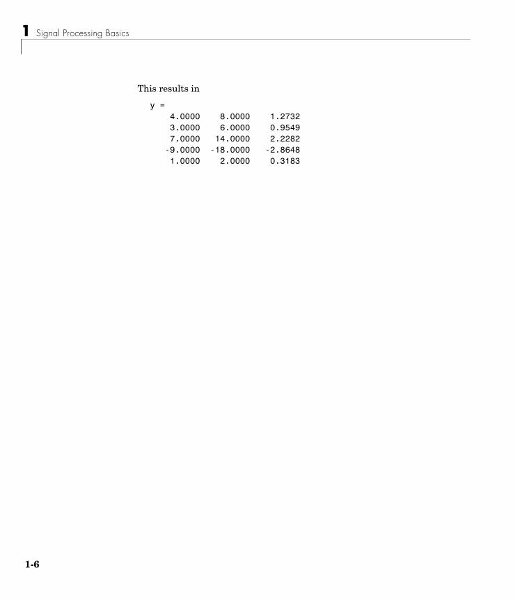
This results in
y =4.0000 8.0000 1.27323.0000 6.0000 0.95497.0000 14.0000 2.2282-9.0000 -18.0000 -2.86481.0000 2.0000 0.3183
Waveform Generation: Time Vectors and Sinusoids
Waveform Generation: Time Vectors and SinusoidsA variety of toolbox functions generate waveforms. Most require you to begin with a vector representing a time base. Consider generating data with a 1000 Hz sample frequency, for example. An appropriate time vector is
t = (0:0.001:1)';
where the MATLAB colon operator creates a 1001-element row vector that represents time running from zero to one second in steps of one millisecond. The transpose operator (') changes the row vector into a column; the semicolon (;) tells MATLAB to compute but not display the result.
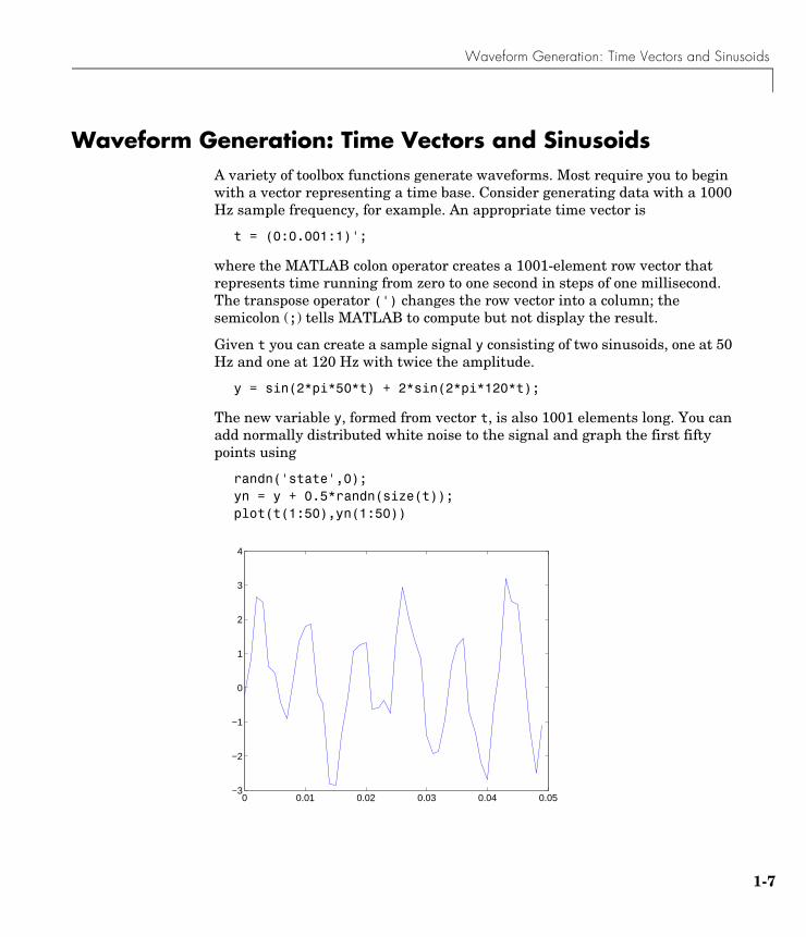
Given t you can create a sample signal y consisting of two sinusoids, one at 50 Hz and one at 120 Hz with twice the amplitude.
y = sin(2*pi*50*t) + 2*sin(2*pi*120*t);
The new variable y, formed from vector t, is also 1001 elements long. You can add normally distributed white noise to the signal and graph the first fifty points using
randn('state',0);yn = y + 0.5*randn(size(t));plot(t(1:50),yn(1:50))
0 0.01 0.02 0.03 0.04 0.05−3
−2
−1
0
1
2
3
4
1-7
1 Signal Processing Basics
1-8
Common Sequences: Unit Impulse, Unit Step, and Unit RampSince MATLAB is a programming language, an endless variety of different signals is possible. Here are some statements that generate several commonly used sequences, including the unit impulse, unit step, and unit ramp functions:
t = (0:0.001:1)';y = [1; zeros(99,1)]; % impulsey = ones(100,1); % step (filter assumes 0 initial cond.)y = t; % rampy = t.^2;y = square(4*t);
All of these sequences are column vectors. The last three inherit their shapes from t.
Multichannel SignalsUse standard MATLAB array syntax to work with multichannel signals. For example, a multichannel signal consisting of the last three signals generated above is
z = [t t.^2 square(4*t)];
You can generate a multichannel unit sample function using the outer product operator. For example, a six-element column vector whose first element is one, and whose remaining five elements are zeros, is
a = [1 zeros(1,5)]';
To duplicate column vector a into a matrix without performing any multiplication, use the MATLAB colon operator and the ones function:
c = a(:,ones(1,3));
Waveform Generation: Time Vectors and Sinusoids
Common Periodic WaveformsThe toolbox provides functions for generating widely used periodic waveforms:
• sawtooth generates a sawtooth wave with peaks at ±1 and a period of . An optional width parameter specifies a fractional multiple of at which the signal’s maximum occurs.
• square generates a square wave with a period of . An optional parameter specifies duty cycle, the percent of the period for which the signal is positive.
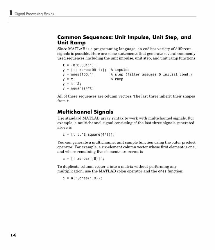
To generate 1.5 seconds of a 50 Hz sawtooth wave with a sample rate of 10 kHz and plot 0.2 seconds of the generated waveform, use
fs = 10000;t = 0:1/fs:1.5;x = sawtooth(2*pi*50*t);plot(t,x), axis([0 0.2 -1 1])
2π2π
2π
0 0.02 0.04 0.06 0.08 0.1 0.12 0.14 0.16 0.18 0.2-1
-0.5
0
0.5
1
1-9
1 Signal Processing Basics
1-1
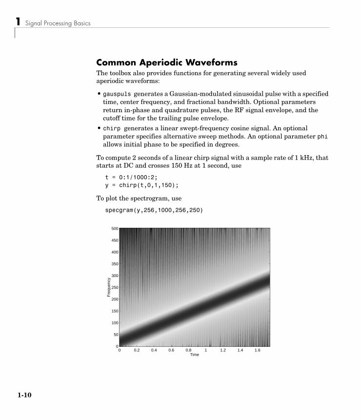
Common Aperiodic WaveformsThe toolbox also provides functions for generating several widely used aperiodic waveforms:
• gauspuls generates a Gaussian-modulated sinusoidal pulse with a specified time, center frequency, and fractional bandwidth. Optional parameters return in-phase and quadrature pulses, the RF signal envelope, and the cutoff time for the trailing pulse envelope.
• chirp generates a linear swept-frequency cosine signal. An optional parameter specifies alternative sweep methods. An optional parameter phi allows initial phase to be specified in degrees.
To compute 2 seconds of a linear chirp signal with a sample rate of 1 kHz, that starts at DC and crosses 150 Hz at 1 second, use
t = 0:1/1000:2;y = chirp(t,0,1,150);
To plot the spectrogram, use
specgram(y,256,1000,256,250)
Time
Fre
quen
cy
0 0.2 0.4 0.6 0.8 1 1.2 1.4 1.60
50
100
150
200
250
300
350
400
450
500
0
Waveform Generation: Time Vectors and Sinusoids
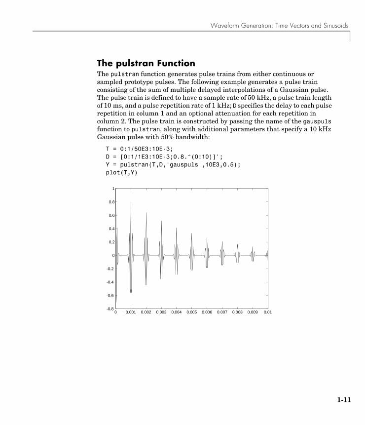
The pulstran FunctionThe pulstran function generates pulse trains from either continuous or sampled prototype pulses. The following example generates a pulse train consisting of the sum of multiple delayed interpolations of a Gaussian pulse. The pulse train is defined to have a sample rate of 50 kHz, a pulse train length of 10 ms, and a pulse repetition rate of 1 kHz; D specifies the delay to each pulse repetition in column 1 and an optional attenuation for each repetition in column 2. The pulse train is constructed by passing the name of the gauspuls function to pulstran, along with additional parameters that specify a 10 kHz Gaussian pulse with 50% bandwidth:
T = 0:1/50E3:10E-3;D = [0:1/1E3:10E-3;0.8.^(0:10)]';Y = pulstran(T,D,'gauspuls',10E3,0.5);plot(T,Y)
0 0.001 0.002 0.003 0.004 0.005 0.006 0.007 0.008 0.009 0.01-0.8
-0.6
-0.4
-0.2
0
0.2
0.4
0.6
0.8
1
1-11
1 Signal Processing Basics
1-1
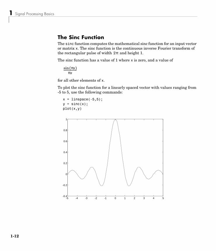
The Sinc FunctionThe sinc function computes the mathematical sinc function for an input vector or matrix x. The sinc function is the continuous inverse Fourier transform of the rectangular pulse of width and height 1.
The sinc function has a value of 1 where x is zero, and a value of
for all other elements of x.
To plot the sinc function for a linearly spaced vector with values ranging from -5 to 5, use the following commands:
x = linspace(-5,5);y = sinc(x);plot(x,y)
2π
πx( )sinπx
--------------------
-5 -4 -3 -2 -1 0 1 2 3 4 5-0.4
-0.2
0
0.2
0.4
0.6
0.8
1
2
Waveform Generation: Time Vectors and Sinusoids
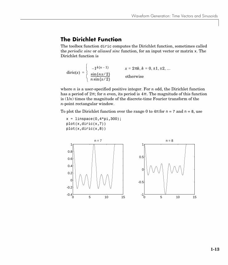
The Dirichlet FunctionThe toolbox function diric computes the Dirichlet function, sometimes called the periodic sinc or aliased sinc function, for an input vector or matrix x. The Dirichlet function is
where n is a user-specified positive integer. For n odd, the Dirichlet function has a period of ; for n even, its period is . The magnitude of this function is (1/n) times the magnitude of the discrete-time Fourier transform of the n-point rectangular window.
To plot the Dirichlet function over the range 0 to 4π for n = 7 and n = 8, use
x = linspace(0,4*pi,300);plot(x,diric(x,7))plot(x,diric(x,8))
diric x( )1– k n 1–( ) x 2πk k 0 1± 2± …, , ,=,=
nx 2⁄( )sinn x 2⁄( )sin---------------------------- otherwise
=
2π 4π
0 5 10 15-0.4
-0.2
0
0.2
0.4
0.6
0.8
1n = 7
0 5 10 15-1
-0.5
0
0.5
1n = 8
1-13
1 Signal Processing Basics
1-1
Working with DataThe examples in the preceding sections obtain data in one of two ways:
• By direct input, that is, entering the data manually at the keyboard
• By using a MATLAB or toolbox function, such as sin, cos, sawtooth, square, or sinc
Some applications, however, may need to import data from outside MATLAB. Depending on your data format, you can do this in the following ways:
• Load data from an ASCII file or MAT-file with the MATLAB load command.
• Read the data into MATLAB with a low-level file I/O function, such as fopen, fread, and fscanf.
• Develop a MEX-file to read the data.
Other resources are also useful, such as a high-level language program (in Fortran or C, for example) that converts your data into MAT-file format – see the MATLAB External Interfaces/API Reference documentation for details. MATLAB reads such files using the load command.
Similar techniques are available for exporting data generated within MATLAB. See the MATLAB documentation for more details on importing and exporting data.
Note Most Signal Processing Toolbox functions accept double-precision inputs. If you have the Filter Design Toolbox installed, you can also use single-precision filtering with dfilt objects.
4
Filter Implementation and Analysis
Filter Implementation and AnalysisThis section describes how to filter discrete signals using the MATLAB filter function and other functions in the Signal Processing Toolbox. It also discusses how to use the toolbox functions to analyze filter characteristics, including impulse response, magnitude and phase response, group delay, and zero-pole locations.
Convolution and FilteringThe mathematical foundation of filtering is convolution. The MATLAB conv function performs standard one-dimensional convolution, convolving one vector with another:
conv([1 1 1],[1 1 1])
ans =
1 2 3 2 1
Note Convolve rectangular matrices for two-dimensional signal processing using the conv2 function.
A digital filter’s output y(k) is related to its input x(k) by convolution with its impulse response h(k).
If a digital filter’s impulse response h(k) is finite length, and the input x(k) is also finite length, you can implement the filter using conv. Store x(k) in a vector x, h(k) in a vector h, and convolve the two:
x = randn(5,1); % A random vector of length 5h = [1 1 1 1]/4; % Length 4 averaging filtery = conv(h,x);
y k( ) h k( ) x k( )∗ h k l–( )x l( )
l ∞–=
∞
∑= =
1-15
1 Signal Processing Basics
1-1
Filters and Transfer FunctionsIn general, the z-transform Y(z) of a digital filter’s output y(n) is related to the z-transform X(z) of the input by
where H(z) is the filter’s transfer function. Here, the constants b(i) and a(i) are the filter coefficients and the order of the filter is the maximum of n and m.
Note The filter coefficients start with subscript 1, rather than 0. This reflects the standard indexing scheme used for vectors in MATLAB.
MATLAB stores the coefficients in two vectors, one for the numerator and one for the denominator. By convention, MATLAB uses row vectors for filter coefficients.
Filter Coefficients and Filter NamesMany standard names for filters reflect the number of a and b coefficients present:
• When n = 0 (that is, b is a scalar), the filter is an Infinite Impulse Response (IIR), all-pole, recursive, or autoregressive (AR) filter.
• When m = 0 (that is, a is a scalar), the filter is a Finite Impulse Response (FIR), all-zero, nonrecursive, or moving-average (MA) filter.
• If both n and m are greater than zero, the filter is an IIR, pole-zero, recursive, or autoregressive moving-average (ARMA) filter.
The acronyms AR, MA, and ARMA are usually applied to filters associated with filtered stochastic processes.
Y z( ) H z( )X z( )b 1( ) b 2( )z 1– b n 1+( )z n–+ + +a 1( ) a 2( )z 1– a m 1+( )z m–+ + +----------------------------------------------------------------------------------------X z( )= =
6
Filter Implementation and Analysis
)
Filtering with the filter FunctionIt is simple to work back to a difference equation from the z-transform relation shown earlier. Assume that a(1) = 1. Move the denominator to the left-hand side and take the inverse z-transform.
In terms of current and past inputs, and past outputs, y(n) is
This is the standard time-domain representation of a digital filter, computed starting with y(1) and assuming zero initial conditions. This representation’s progression is
A filter in this form is easy to implement with the filter function. For example, a simple single-pole filter (lowpass) is
b = 1; % Numeratora = [1 -0.9]; % Denominator
where the vectors b and a represent the coefficients of a filter in transfer function form. To apply this filter to your data, use
y = filter(b,a,x);
filter gives you as many output samples as there are input samples, that is, the length of y is the same as the length of x. If the first element of a is not 1, filter divides the coefficients by a(1) before implementing the difference equation.
y k( ) a2y k 1–( ) am 1+ y k m–( )+ + + b1x k( ) b2x k 1–( ) bn 1+ x k m–(+ + +=
y k( ) b1x k( ) b2x k 1–( ) bn 1+ x k n–( ) a2y k 1–( )– am 1+ y k n–( )––+ + +=
y 1( ) b1x 1( )=
y 2( ) b1x 2( ) b2x 1( ) a2y 1( )–+=
y 3( ) b1x 3( ) b2x 2( ) b3x 1( ) a2y 2( ) a3y 1( )––+ +=
=
1-17
1 Signal Processing Basics
1-1
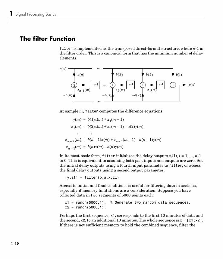
The filter Function filter is implemented as the transposed direct-form II structure, where n-1 is the filter order. This is a canonical form that has the minimum number of delay elements.
At sample m, filter computes the difference equations
In its most basic form, filter initializes the delay outputs zi(1), i = 1, ..., n-1 to 0. This is equivalent to assuming both past inputs and outputs are zero. Set the initial delay outputs using a fourth input parameter to filter, or access the final delay outputs using a second output parameter:
[y,zf] = filter(b,a,x,zi)
Access to initial and final conditions is useful for filtering data in sections, especially if memory limitations are a consideration. Suppose you have collected data in two segments of 5000 points each:
x1 = randn(5000,1); % Generate two random data sequences.x2 = randn(5000,1);
Perhaps the first sequence, x1, corresponds to the first 10 minutes of data and the second, x2, to an additional 10 minutes. The whole sequence is x = [x1;x2]. If there is not sufficient memory to hold the combined sequence, filter the
Σ Σ Σz -1 z -1
x(m)
y(m)
b(3) b(2) b(1)
– a(3) – a(2)
z1(m)z2(m)Σ z -1
b(n)
–a(n)
zn -1(m)
...
...
...
y m( ) b 1( )x m( ) z1 m 1–( )+=
z1 m( ) b 2( )x m( ) z2 m 1–( ) a 2( )y m( )–+=
=
zn 2– m( ) b n 1–( )x m( ) zn 1– m 1–( ) a n 1–( )y m( )–+=
zn 1– m( ) b n( )x m( ) a n( )y m( )–=
8
The filter Function
subsequences x1 and x2 one at a time. To ensure continuity of the filtered sequences, use the final conditions from x1 as initial conditions to filter x2:
[y1,zf] = filter(b,a,x1);y2 = filter(b,a,x2,zf);
The filtic function generates initial conditions for filter. filtic computes the delay vector to make the behavior of the filter reflect past inputs and outputs that you specify. To obtain the same output delay values zf as above using filtic, use
zf = filtic(b,a,flipud(y1),flipud(x1));
This can be useful when filtering short data sequences, as appropriate initial conditions help reduce transient startup effects.
1-19
1 Signal Processing Basics
1-2
Other Functions for FilteringIn addition to filter, several other functions in the Signal Processing Toolbox perform the basic filtering operation. These functions include upfirdn, which performs FIR filtering with resampling, filtfilt, which eliminates phase distortion in the filtering process, fftfilt, which performs the FIR filtering operation in the frequency domain, and latcfilt, which filters using a lattice implementation.
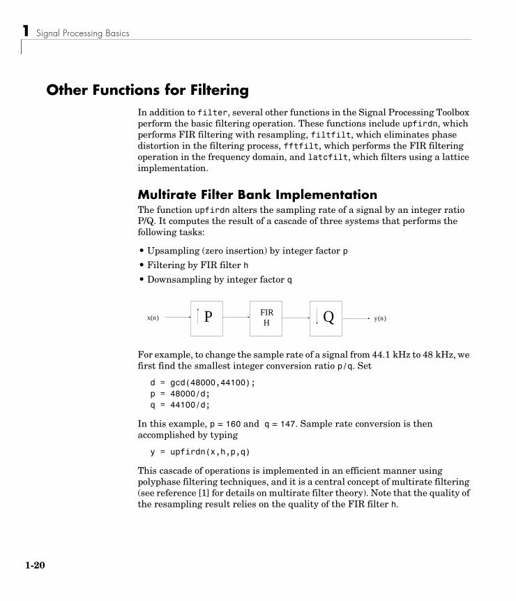
Multirate Filter Bank ImplementationThe function upfirdn alters the sampling rate of a signal by an integer ratioP/Q. It computes the result of a cascade of three systems that performs the following tasks:
• Upsampling (zero insertion) by integer factor p
• Filtering by FIR filter h
• Downsampling by integer factor q
For example, to change the sample rate of a signal from 44.1 kHz to 48 kHz, we first find the smallest integer conversion ratio p/q. Set
d = gcd(48000,44100);p = 48000/d;q = 44100/d;
In this example, p = 160 and q = 147. Sample rate conversion is then accomplished by typing
y = upfirdn(x,h,p,q)
This cascade of operations is implemented in an efficient manner using polyphase filtering techniques, and it is a central concept of multirate filtering (see reference [1] for details on multirate filter theory). Note that the quality of the resampling result relies on the quality of the FIR filter h.
Px(n) y(n)FIRH Q
0
Other Functions for Filtering
Filter banks may be implemented using upfirdn by allowing the filter h to be a matrix, with one FIR filter per column. A signal vector is passed independently through each FIR filter, resulting in a matrix of output signals.
Other functions that perform multirate filtering (with fixed filter) include resample, interp, and decimate.
Anti-Causal, Zero-Phase Filter ImplementationIn the case of FIR filters, it is possible to design linear phase filters that, when applied to data (using filter or conv), simply delay the output by a fixed number of samples. For IIR filters, however, the phase distortion is usually highly nonlinear. The filtfilt function uses the information in the signal at points before and after the current point, in essence “looking into the future,” to eliminate phase distortion.
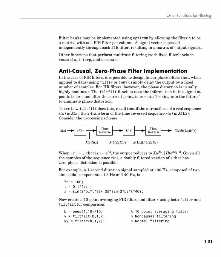
To see how filtfilt does this, recall that if the z-transform of a real sequence x(n) is X(z), the z-transform of the time reversed sequence x(n) is X(1/z). Consider the processing scheme.
When |z| = 1, that is z = ejω, the output reduces to X(ejω)|H(ejω)|2. Given all the samples of the sequence x(n), a doubly filtered version of x that has zero-phase distortion is possible.
For example, a 1-second duration signal sampled at 100 Hz, composed of two sinusoidal components at 3 Hz and 40 Hz, is
fs = 100;t = 0:1/fs:1;x = sin(2*pi*t*3)+.25*sin(2*pi*t*40);
Now create a 10-point averaging FIR filter, and filter x using both filter and filtfilt for comparison:
b = ones(1,10)/10; % 10 point averaging filtery = filtfilt(b,1,x); % Noncausal filteringyy = filter(b,1,x); % Normal filtering
H(z)X(z)
X(z)H(z) X(1/z)H(1/z) X(1/z)H(1/z)H(z)
X(z)H(1/z)H(z)H(z)TimeReverse
TimeReverse
1-21
1 Signal Processing Basics
1-2
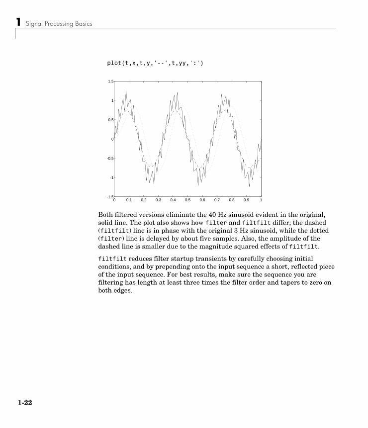
plot(t,x,t,y,'--',t,yy,':')
Both filtered versions eliminate the 40 Hz sinusoid evident in the original, solid line. The plot also shows how filter and filtfilt differ; the dashed (filtfilt) line is in phase with the original 3 Hz sinusoid, while the dotted (filter) line is delayed by about five samples. Also, the amplitude of the dashed line is smaller due to the magnitude squared effects of filtfilt.
filtfilt reduces filter startup transients by carefully choosing initial conditions, and by prepending onto the input sequence a short, reflected piece of the input sequence. For best results, make sure the sequence you are filtering has length at least three times the filter order and tapers to zero on both edges.
0 0.1 0.2 0.3 0.4 0.5 0.6 0.7 0.8 0.9 1-1.5
-1
-0.5
0
0.5
1
1.5
2
Other Functions for Filtering
Frequency Domain Filter ImplementationDuality between the time domain and the frequency domain makes it possible to perform any operation in either domain. Usually one domain or the other is more convenient for a particular operation, but you can always accomplish a given operation in either domain.
To implement general IIR filtering in the frequency domain, multiply the discrete Fourier transform (DFT) of the input sequence with the quotient of the DFT of the filter:
n = length(x);y = ifft(fft(x).*fft(b,n)./fft(a,n));
This computes results that are identical to filter, but with different startup transients (edge effects). For long sequences, this computation is very inefficient because of the large zero-padded FFT operations on the filter coefficients, and because the FFT algorithm becomes less efficient as the number of points n increases.
For FIR filters, however, it is possible to break longer sequences into shorter, computationally efficient FFT lengths. The function
y = fftfilt(b,x)
uses the overlap add method (see reference [1] at the end of this chapter) to filter a long sequence with multiple medium-length FFTs. Its output is equivalent to filter(b,1,x).
1-23
1 Signal Processing Basics
1-2
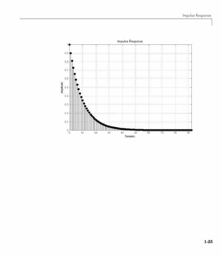
Impulse ResponseThe impulse response of a digital filter is the output arising from the unit impulse input sequence defined as
In MATLAB, you can generate an impulse sequence a number of ways; one straightforward way is
imp = [1; zeros(49,1)];
The impulse response of the simple filter b = 1 and a = [1 -0.9] is
h = filter(b,a,imp);
A simple way to display the impulse response is with the Filter Visualization Tool (fvtool):
fvtool(b,a)
Then click the Impulse Response button on the toolbar or select Impulse Response from the Analysis menu. This plot shows the exponential decay h(n) = 0.9n of the single pole system:
x n( )1 n 1=,0 n 1≠,
=
4
Impulse Response
1-25
1 Signal Processing Basics
1-2
Frequency ResponseThe Signal Processing Toolbox enables you to perform frequency domain analysis of both analog and digital filters.
Digital Domainfreqz uses an FFT-based algorithm to calculate the z-transform frequency response of a digital filter. Specifically, the statement
[h,w] = freqz(b,a,p)
returns the p-point complex frequency response, , of the digital filter.
In its simplest form, freqz accepts the filter coefficient vectors b and a, and an integer p specifying the number of points at which to calculate the frequency response. freqz returns the complex frequency response in vector h, and the actual frequency points in vector w in rad/s.
freqz can accept other parameters, such as a sampling frequency or a vector of arbitrary frequency points. The example below finds the 256-point frequency response for a 12th-order Chebyshev Type I filter. The call to freqz specifies a sampling frequency fs of 1000 Hz:
[b,a] = cheby1(12,0.5,200/500);[h,f] = freqz(b,a,256,1000);
Because the parameter list includes a sampling frequency, freqz returns a vector f that contains the 256 frequency points between 0 and fs/2 used in the frequency response calculation.
H ejω( )
H ejω( )b 1( ) b 2( )e j– ω b n 1+( )e j– ω n( )+ + +
a 1( ) a 2( )e j– ω a m 1+( )e j– ω m( )+ + +---------------------------------------------------------------------------------------------------=
6
Frequency Response
Note This toolbox uses the convention that unit frequency is the Nyquist frequency, defined as half the sampling frequency. The cutoff frequency parameter for all basic filter design functions is normalized by the Nyquist frequency. For a system with a 1000 Hz sampling frequency, for example, 300 Hz is 300/500 = 0.6. To convert normalized frequency to angular frequency around the unit circle, multiply by π. To convert normalized frequency back to hertz, multiply by half the sample frequency.
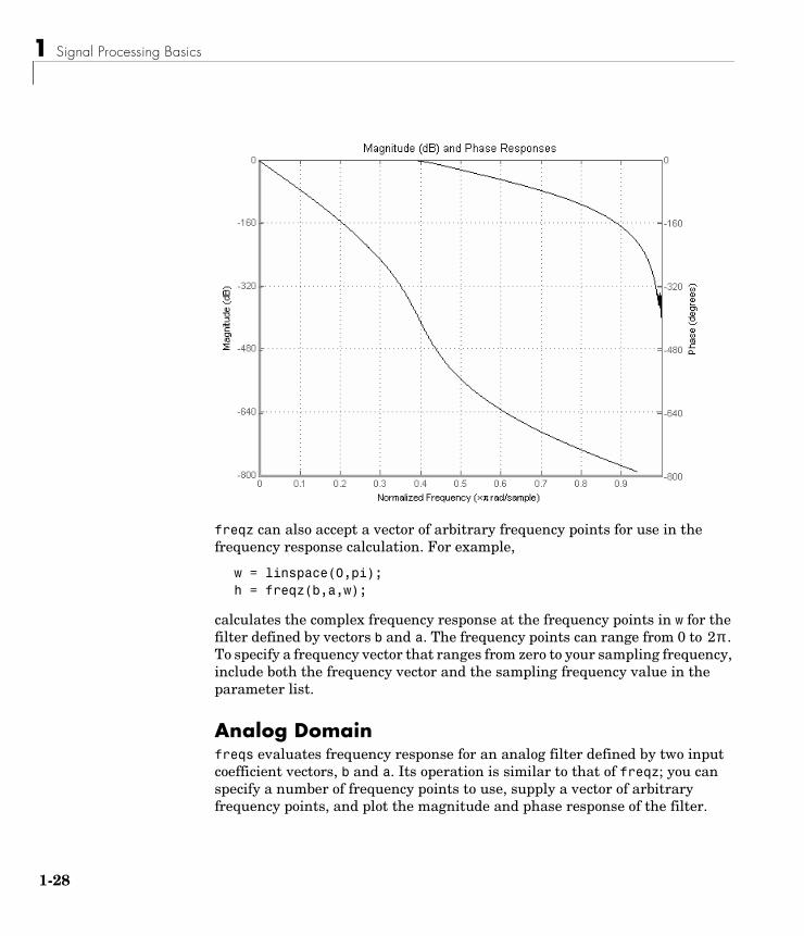
If you call freqz with no output arguments, it plots both magnitude versus frequency and phase versus frequency. For example, a ninth-order Butterworth lowpass filter with a cutoff frequency of 400 Hz, based on a 2000 Hz sampling frequency, is
[b,a] = butter(9,400/1000);
To calculate the 256-point complex frequency response for this filter, and plot the magnitude and phase with freqz, use
freqz(b,a,256,2000)
or to display the magnitude and phase responses in fvtool, which provides additional analysis tools, use
fvtool(b,a)
and click the Magnitude and Phase Response button on the toolbar or select Magnitude and Phase Response from the Analysis menu.
1-27
1 Signal Processing Basics
1-2
freqz can also accept a vector of arbitrary frequency points for use in the frequency response calculation. For example,
w = linspace(0,pi);h = freqz(b,a,w);
calculates the complex frequency response at the frequency points in w for the filter defined by vectors b and a. The frequency points can range from 0 to . To specify a frequency vector that ranges from zero to your sampling frequency, include both the frequency vector and the sampling frequency value in the parameter list.
Analog Domainfreqs evaluates frequency response for an analog filter defined by two input coefficient vectors, b and a. Its operation is similar to that of freqz; you can specify a number of frequency points to use, supply a vector of arbitrary frequency points, and plot the magnitude and phase response of the filter.
2π
8
Frequency Response
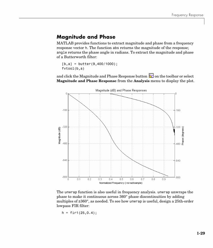
Magnitude and PhaseMATLAB provides functions to extract magnitude and phase from a frequency response vector h. The function abs returns the magnitude of the response; angle returns the phase angle in radians. To extract the magnitude and phase of a Butterworth filter:
[b,a] = butter(9,400/1000);fvtool(b,a)
and click the Magnitude and Phase Response button on the toolbar or select Magnitude and Phase Response from the Analysis menu to display the plot.
The unwrap function is also useful in frequency analysis. unwrap unwraps the phase to make it continuous across 360° phase discontinuities by adding multiples of ±360°, as needed. To see how unwrap is useful, design a 25th-order lowpass FIR filter:
h = fir1(25,0.4);
1-29
1 Signal Processing Basics
1-3
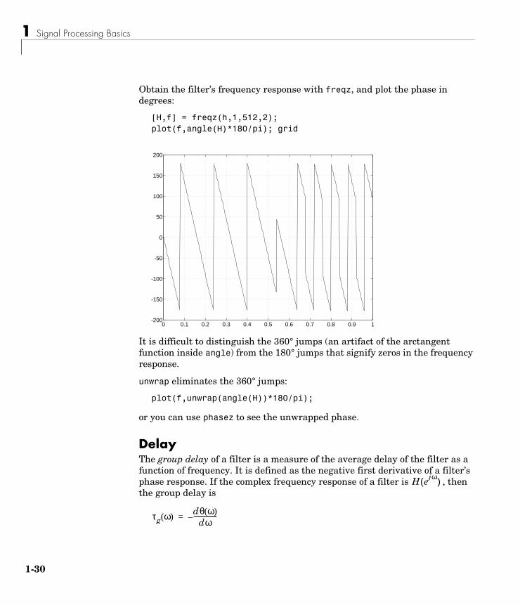
Obtain the filter’s frequency response with freqz, and plot the phase in degrees:
[H,f] = freqz(h,1,512,2);plot(f,angle(H)*180/pi); grid
It is difficult to distinguish the 360° jumps (an artifact of the arctangent function inside angle) from the 180° jumps that signify zeros in the frequency response.
unwrap eliminates the 360° jumps:
plot(f,unwrap(angle(H))*180/pi);
or you can use phasez to see the unwrapped phase.
DelayThe group delay of a filter is a measure of the average delay of the filter as a function of frequency. It is defined as the negative first derivative of a filter’s phase response. If the complex frequency response of a filter is , then the group delay is
0 0.1 0.2 0.3 0.4 0.5 0.6 0.7 0.8 0.9 1-200
-150
-100
-50
0
50
100
150
200
H ejω( )
τg ω( )dθ ω( )
dω---------------–=
0
Frequency Response
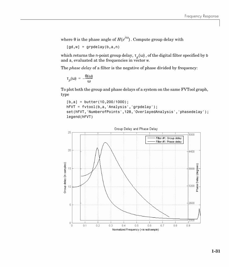
where θ is the phase angle of . Compute group delay with
[gd,w] = grpdelay(b,a,n)
which returns the n-point group delay, , of the digital filter specified by b and a, evaluated at the frequencies in vector w.
The phase delay of a filter is the negative of phase divided by frequency:
To plot both the group and phase delays of a system on the same FVTool graph, type
[b,a] = butter(10,200/1000); hFVT = fvtool(b,a,'Analysis','grpdelay'); set(hFVT,'NumberofPoints',128,'OverlayedAnalysis','phasedelay'); legend(hFVT)
H ejω( )
τg ω( )
τp ω( )θ ω( )
ω-----------–=
1-31

1 Signal Processing Basics
1-3
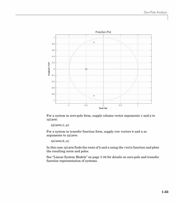
Zero-Pole AnalysisThe zplane function plots poles and zeros of a linear system. For example, a simple filter with a zero at -1/2 and a complex pole pair at and
is
zer = -0.5; pol = 0.9*exp(j*2*pi*[-0.3 0.3]');
To view the pole-zero plot for this filter you can use
zplane(zer,pol)
or, for access to additional tools, use fvtool. First convert the poles and zeros to transfer function form, then call fvtool,
[b,a] = zp2tf(zer,pol,1);fvtool(b,a)
and click the Pole/Zero Plot toolbar button on the toolbar or select Pole/Zero Plot from the Analysis menu to see the plot.
0.9ej2π 0.3( )
0.9e j– 2π 0.3( )
2
Zero-Pole Analysis
For a system in zero-pole form, supply column vector arguments z and p to zplane:
zplane(z,p)
For a system in transfer function form, supply row vectors b and a as arguments to zplane:
zplane(b,a)
In this case zplane finds the roots of b and a using the roots function and plots the resulting zeros and poles.
See “Linear System Models” on page 1-34 for details on zero-pole and transfer function representation of systems.
1-33
1 Signal Processing Basics
1-3
Linear System ModelsThe Signal Processing Toolbox provides several models for representing linear time-invariant systems. This flexibility lets you choose the representational scheme that best suits your application and, within the bounds of numeric stability, convert freely to and from most other models. This section provides a brief overview of supported linear system models and describes how to work with these models in MATLAB.
Discrete-Time System ModelsThe discrete-time system models are representational schemes for digital filters. MATLAB supports several discrete-time system models, which are described in the following sections:
• “Transfer Function”
• “Zero-Pole-Gain”
• “State-Space”
• “Partial Fraction Expansion (Residue Form)”
• “Second-Order Sections (SOS)”
• “Lattice Structure”
• “Convolution Matrix”
Transfer FunctionThe transfer function is a basic z-domain representation of a digital filter, expressing the filter as a ratio of two polynomials. It is the principal discrete-time model for this toolbox. The transfer function model description for the z-transform of a digital filter’s difference equation is
Here, the constants b(i) and a(i) are the filter coefficients, and the order of the filter is the maximum of n and m. In MATLAB, you store these coefficients in two vectors (row vectors by convention), one row vector for the numerator and one for the denominator. See “Filters and Transfer Functions” on page 1-16 for more details on the transfer function form.
Y z( )b 1( ) b 2( )z 1– b n 1+( )z n–+ + +a 1( ) a 2( )z 1– a m 1+( )z m–+ + +----------------------------------------------------------------------------------------X z( )=
4
Linear System Models
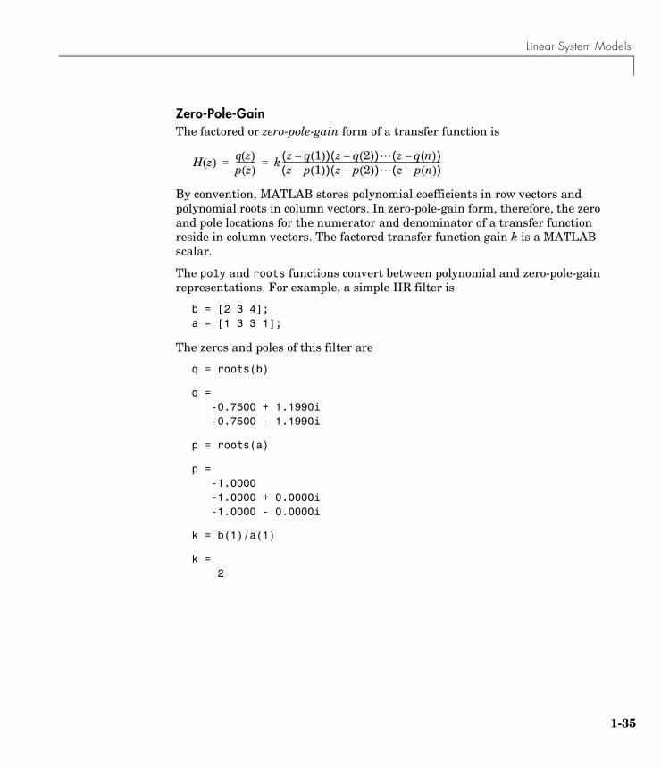
Zero-Pole-GainThe factored or zero-pole-gain form of a transfer function is
By convention, MATLAB stores polynomial coefficients in row vectors and polynomial roots in column vectors. In zero-pole-gain form, therefore, the zero and pole locations for the numerator and denominator of a transfer function reside in column vectors. The factored transfer function gain k is a MATLAB scalar.
The poly and roots functions convert between polynomial and zero-pole-gain representations. For example, a simple IIR filter is
b = [2 3 4];a = [1 3 3 1];
The zeros and poles of this filter are
q = roots(b)
q =-0.7500 + 1.1990i-0.7500 - 1.1990i
p = roots(a)
p =-1.0000-1.0000 + 0.0000i-1.0000 - 0.0000i
k = b(1)/a(1)
k =2
H z( )q z( )p z( )---------- k z q 1( )–( ) z q 2( )–( ) z q n( )–( )
z p 1( )–( ) z p 2( )–( ) z p n( )–( )--------------------------------------------------------------------------------= =
1-35
1 Signal Processing Basics
1-3
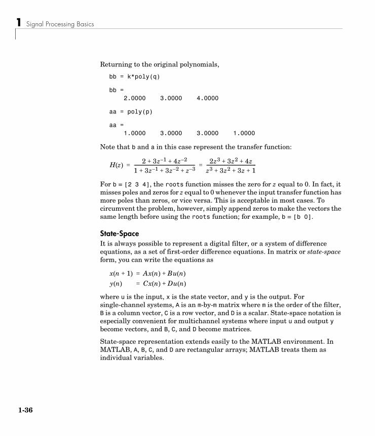
Returning to the original polynomials,
bb = k*poly(q)
bb =2.0000 3.0000 4.0000
aa = poly(p)
aa =1.0000 3.0000 3.0000 1.0000
Note that b and a in this case represent the transfer function:
For b = [2 3 4], the roots function misses the zero for z equal to 0. In fact, it misses poles and zeros for z equal to 0 whenever the input transfer function has more poles than zeros, or vice versa. This is acceptable in most cases. To circumvent the problem, however, simply append zeros to make the vectors the same length before using the roots function; for example, b = [b 0].
State-SpaceIt is always possible to represent a digital filter, or a system of difference equations, as a set of first-order difference equations. In matrix or state-space form, you can write the equations as
where u is the input, x is the state vector, and y is the output. For single-channel systems, A is an m-by-m matrix where m is the order of the filter, B is a column vector, C is a row vector, and D is a scalar. State-space notation is especially convenient for multichannel systems where input u and output y become vectors, and B, C, and D become matrices.
State-space representation extends easily to the MATLAB environment. In MATLAB, A, B, C, and D are rectangular arrays; MATLAB treats them as individual variables.
H z( )2 3z 1– 4z 2–+ +
1 3z 1– 3z 2– z 3–+ + +------------------------------------------------------ 2z3 3z2 4z+ +
z3 3z2 3z 1+ + +--------------------------------------------= =
x n 1+( ) Ax n( ) Bu n( )+=
y n( ) Cx n( ) Du n( )+=
6
Linear System Models
Taking the z-transform of the state-space equations and combining them shows the equivalence of state-space and transfer function forms:
Don’t be concerned if you are not familiar with the state-space representation of linear systems. Some of the filter design algorithms use state-space form internally but do not require any knowledge of state-space concepts to use them successfully. If your applications use state-space based signal processing extensively, however, consult the Contr ol System Toolbox for a comprehensive library of state-space tools.
Partial Fraction Expansion (Residue Form)Each transfer function also has a corresponding partial fraction expansion or residue form representation, given by
provided H(z) has no repeated poles. Here, n is the degree of the denominator polynomial of the rational transfer function b(z)/a(z). If r is a pole of multiplicity sr, then H(z) has terms of the form:
The residuez function in the Signal Processing Toolbox converts transfer functions to and from the partial fraction expansion form. The “z” on the end of residuez stands for z-domain, or discrete domain. residuez returns the poles in a column vector p, the residues corresponding to the poles in a column vector r, and any improper part of the original transfer function in a row vector k. residuez determines that two poles are the same if the magnitude of their difference is smaller than 0.1 percent of either of the poles’ magnitudes.
Y z( ) H z( )U z( )= where H z( ) C zI A–( ) 1– B D+=,
b z( )a z( )---------- r 1( )
1 p 1( )z 1––---------------------------- r n( )
1 p n( )z 1––----------------------------- k 1( ) k 2( )z 1– k m n 1+–( )z m n–( )–+ + + + + +=
r j( )
1 p j( )z 1––--------------------------- r j 1+( )
1 p j( )z 1––( )2-----------------------------------
r j sr 1–+( )
1 p j( )z 1––( )sr------------------------------------+ + +
1-37
1 Signal Processing Basics
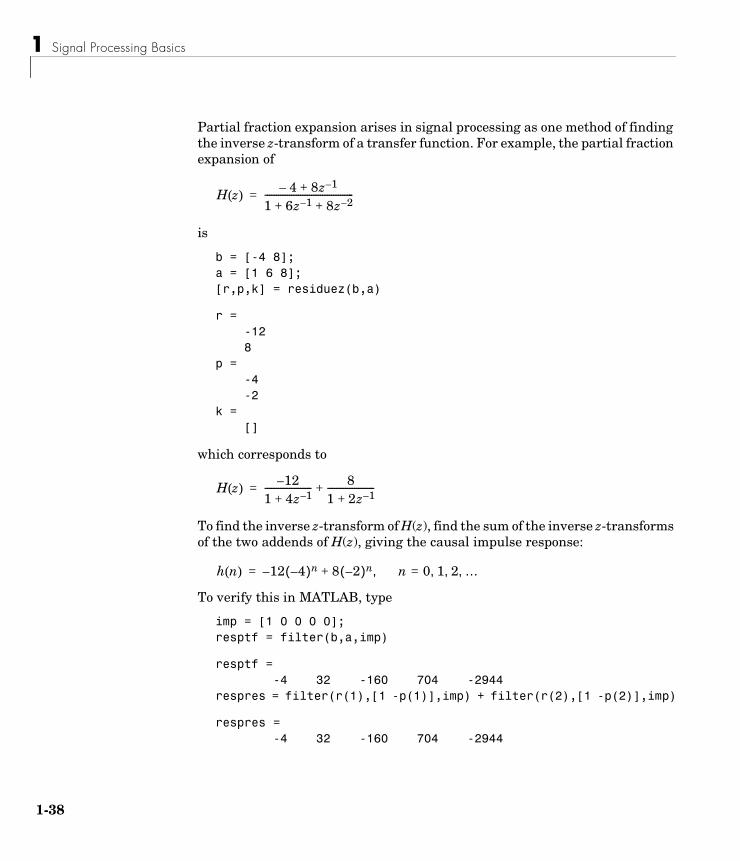
1-3
Partial fraction expansion arises in signal processing as one method of finding the inverse z-transform of a transfer function. For example, the partial fraction expansion of
is
b = [-4 8];a = [1 6 8];[r,p,k] = residuez(b,a)
r =-128
p =-4-2
k =[]
which corresponds to
To find the inverse z-transform of H(z), find the sum of the inverse z-transforms of the two addends of H(z), giving the causal impulse response:
To verify this in MATLAB, type
imp = [1 0 0 0 0];resptf = filter(b,a,imp)
resptf =-4 32 -160 704 -2944
respres = filter(r(1),[1 -p(1)],imp) + filter(r(2),[1 -p(2)],imp)
respres =-4 32 -160 704 -2944
H z( )4– 8z 1–+
1 6z 1– 8z 2–+ +----------------------------------------=
H z( )12–
1 4z 1–+--------------------- 8
1 2z 1–+---------------------+=
h n( ) 12– 4–( )n 8 2–( )n+ n 0 1 2 …, , ,=,=
8
Linear System Models
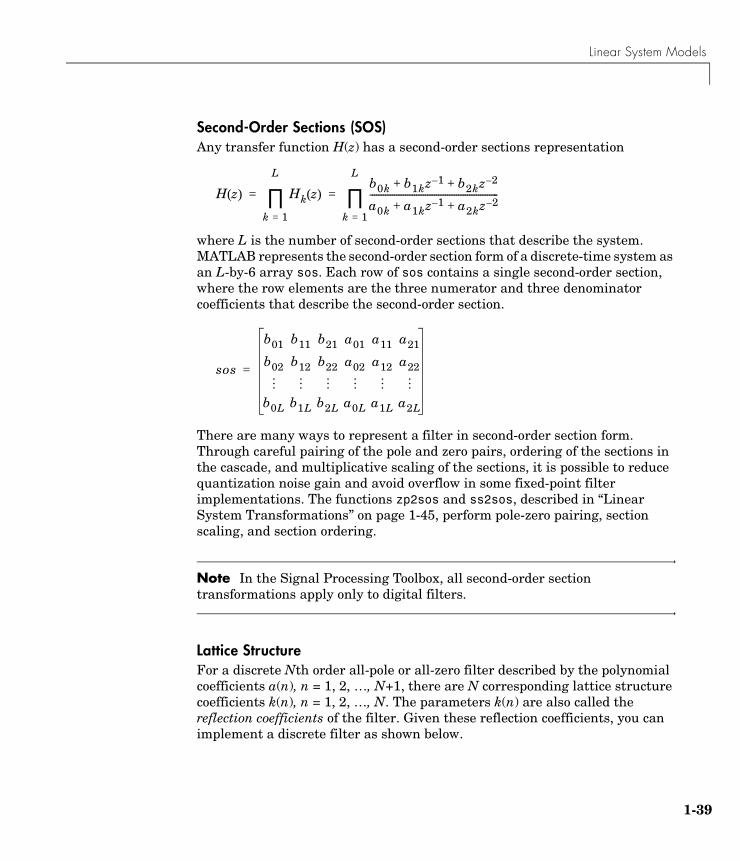
Second-Order Sections (SOS)Any transfer function H(z) has a second-order sections representation
where L is the number of second-order sections that describe the system. MATLAB represents the second-order section form of a discrete-time system as an L-by-6 array sos. Each row of sos contains a single second-order section, where the row elements are the three numerator and three denominator coefficients that describe the second-order section.
There are many ways to represent a filter in second-order section form. Through careful pairing of the pole and zero pairs, ordering of the sections in the cascade, and multiplicative scaling of the sections, it is possible to reduce quantization noise gain and avoid overflow in some fixed-point filter implementations. The functions zp2sos and ss2sos, described in “Linear System Transformations” on page 1-45, perform pole-zero pairing, section scaling, and section ordering.
Note In the Signal Processing Toolbox, all second-order section transformations apply only to digital filters.
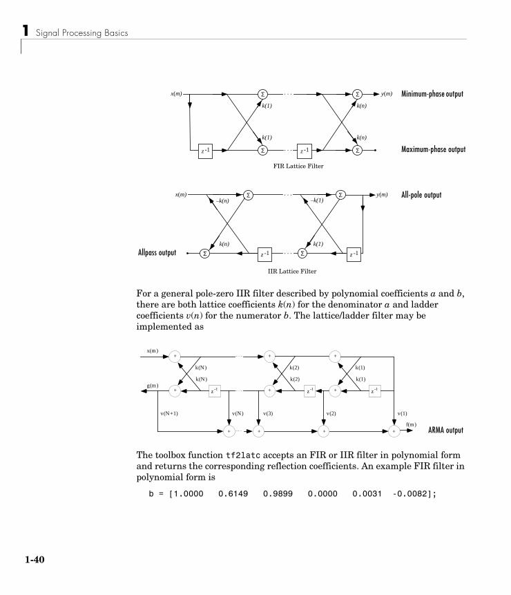
Lattice StructureFor a discrete Nth order all-pole or all-zero filter described by the polynomial coefficients a(n), n = 1, 2, …, N+1, there are N corresponding lattice structure coefficients k(n), n = 1, 2, …, N. The parameters k(n) are also called the reflection coefficients of the filter. Given these reflection coefficients, you can implement a discrete filter as shown below.
H z( ) Hk z( )
k 1=
L
∏b0k b1kz 1– b2kz 2–+ +
a0k a1kz 1– a2kz 2–+ +----------------------------------------------------------
k 1=
L
∏= =
sos
b01 b11 b21 a01 a11 a21
b02 b12 b22 a02 a12 a22
b0L b1L b2L a0L a1L a2L
=
1-39
1 Signal Processing Basics
1-4
For a general pole-zero IIR filter described by polynomial coefficients a and b, there are both lattice coefficients k(n) for the denominator a and ladder coefficients v(n) for the numerator b. The lattice/ladder filter may be implemented as
The toolbox function tf2latc accepts an FIR or IIR filter in polynomial form and returns the corresponding reflection coefficients. An example FIR filter in polynomial form is
b = [1.0000 0.6149 0.9899 0.0000 0.0031 -0.0082];
Σ
Σ
z -1
y(m)
k(1)
k(1)
Σ
Σ
k(n)
k(n)
. . .
. . . z -1
FIR Lattice Filter
x(m)
x(m)
Σ
Σ y(m)
k(1)
–k(1)Σ
k(n)
–k(n). . .
. . .z -1 Σ z -1
IIR Lattice Filter
Minimum-phase output
All-pole output
Maximum-phase output
Allpass output
z-1+
+x(m)
g(m)
+
k(N)
k(N)
z-1+
+
k(2)
k(2)
z-1+
+
k(1)
k(1)
++ +
v(N+1) v(N) v(3) v(2) v(1)
f(m)ARMA output
0
Linear System Models
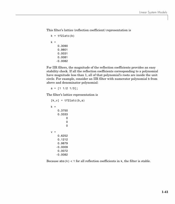
This filter’s lattice (reflection coefficient) representation is
k = tf2latc(b)
k = 0.3090
0.98010.00310.0081-0.0082
For IIR filters, the magnitude of the reflection coefficients provides an easy stability check. If all the reflection coefficients corresponding to a polynomial have magnitude less than 1, all of that polynomial’s roots are inside the unit circle. For example, consider an IIR filter with numerator polynomial b from above and denominator polynomial:
a = [1 1/2 1/3];
The filter’s lattice representation is
[k,v] = tf2latc(b,a)
k = 0.3750 0.3333 0 0 0
v = 0.6252 0.1212 0.9879 -0.0009 0.0072 -0.0082
Because abs(k) < 1 for all reflection coefficients in k, the filter is stable.
1-41
1 Signal Processing Basics
1-4
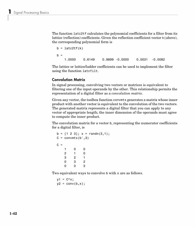
The function latc2tf calculates the polynomial coefficients for a filter from its lattice (reflection) coefficients. Given the reflection coefficient vector k(above), the corresponding polynomial form is
b = latc2tf(k)
b = 1.0000 0.6149 0.9899 -0.0000 0.0031 -0.0082
The lattice or lattice/ladder coefficients can be used to implement the filter using the function latcfilt.
Convolution MatrixIn signal processing, convolving two vectors or matrices is equivalent to filtering one of the input operands by the other. This relationship permits the representation of a digital filter as a convolution matrix.
Given any vector, the toolbox function convmtx generates a matrix whose inner product with another vector is equivalent to the convolution of the two vectors. The generated matrix represents a digital filter that you can apply to any vector of appropriate length; the inner dimension of the operands must agree to compute the inner product.
The convolution matrix for a vector b, representing the numerator coefficients for a digital filter, is
b = [1 2 3]; x = randn(3,1);C = convmtx(b',3)
C =1 0 02 1 03 2 10 3 20 0 3
Two equivalent ways to convolve b with x are as follows.
y1 = C*x;y2 = conv(b,x);
2
Linear System Models
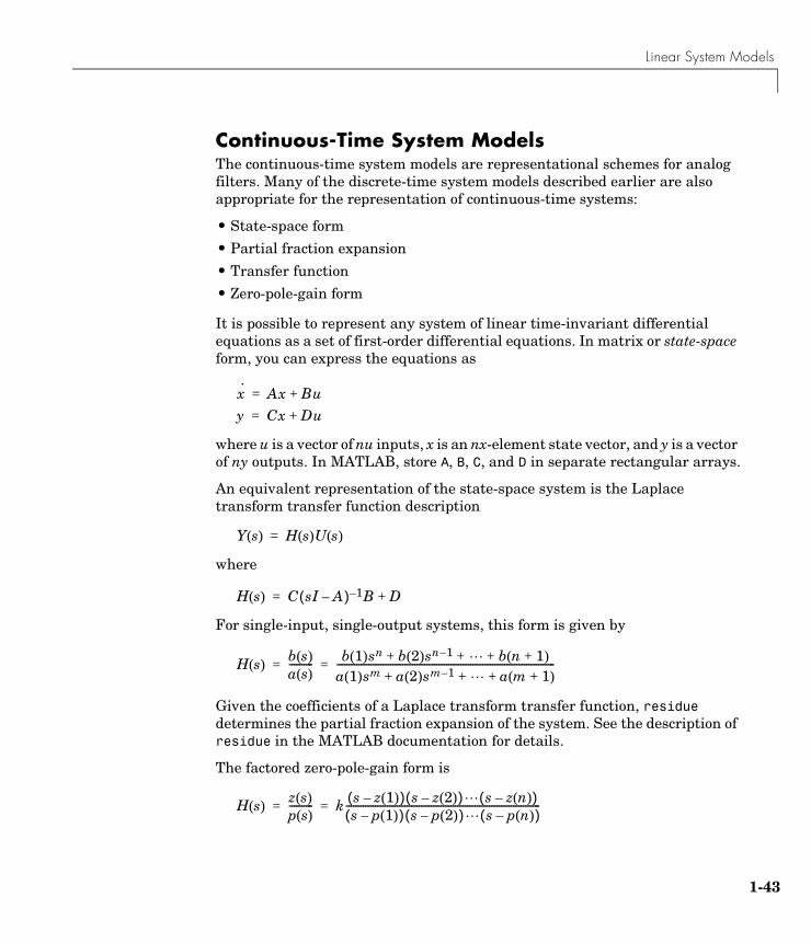
Continuous-Time System ModelsThe continuous-time system models are representational schemes for analog filters. Many of the discrete-time system models described earlier are also appropriate for the representation of continuous-time systems:
• State-space form
• Partial fraction expansion
• Transfer function
• Zero-pole-gain form
It is possible to represent any system of linear time-invariant differential equations as a set of first-order differential equations. In matrix or state-space form, you can express the equations as
where u is a vector of nu inputs, x is an nx-element state vector, and y is a vector of ny outputs. In MATLAB, store A, B, C, and D in separate rectangular arrays.
An equivalent representation of the state-space system is the Laplace transform transfer function description
where
For single-input, single-output systems, this form is given by
Given the coefficients of a Laplace transform transfer function, residue determines the partial fraction expansion of the system. See the description of residue in the MATLAB documentation for details.
The factored zero-pole-gain form is
x·
Ax Bu+=
y Cx Du+=
Y s( ) H s( )U s( )=
H s( ) C sI A–( ) 1– B D+=
H s( )b s( )a s( )---------- b 1( )sn b 2( )sn 1– b n 1+( )+ + +
a 1( )sm a 2( )sm 1– a m 1+( )+ + +------------------------------------------------------------------------------------------= =
H s( )z s( )p s( )---------- k s z 1( )–( ) s z 2( )–( ) s z n( )–( )
s p 1( )–( ) s p 2( )–( ) s p n( )–( )--------------------------------------------------------------------------------= =
1-43
1 Signal Processing Basics
1-4
As in the discrete-time case, MATLAB stores polynomial coefficients in row vectors in descending powers of s. MATLAB stores polynomial roots, or zeros and poles, in column vectors.
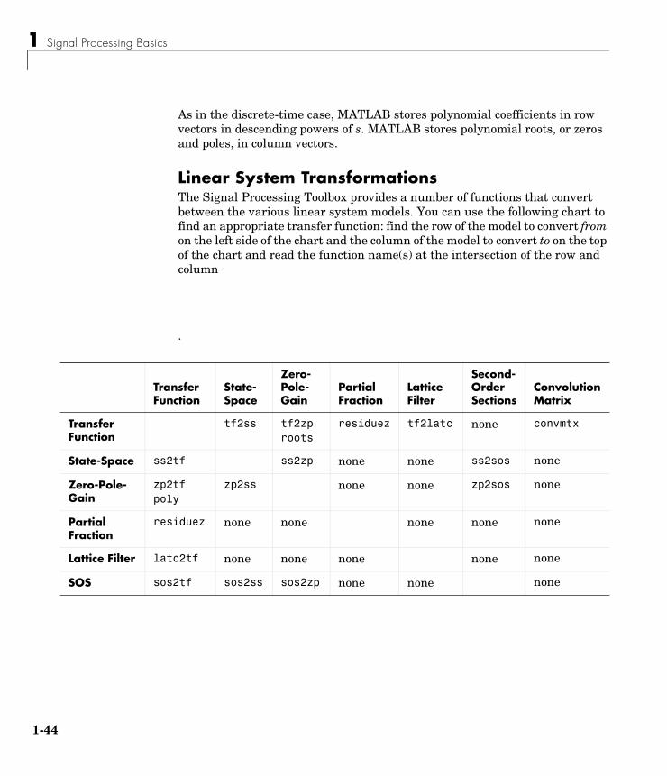
Linear System TransformationsThe Signal Processing Toolbox provides a number of functions that convert between the various linear system models. You can use the following chart to find an appropriate transfer function: find the row of the model to convert from on the left side of the chart and the column of the model to convert to on the top of the chart and read the function name(s) at the intersection of the row and column
.
Transfer Function
State- Space
Zero-Pole-Gain
Partial Fraction
Lattice Filter
Second-Order Sections
ConvolutionMatrix
Transfer Function
tf2ss tf2zp roots
residuez tf2latc none convmtx
State-Space ss2tf ss2zp none none ss2sos none
Zero-Pole- Gain
zp2tf poly
zp2ss none none zp2sos none
Partial Fraction
residuez none none none none none
Lattice Filter latc2tf none none none none none
SOS sos2tf sos2ss sos2zp none none none
4
Linear System Models
Note Converting from one filter structure or model to another may produce a result with different characteristics than the original. This is due to the computer’s finite-precision arithmetic and the variations in the conversion’s round-off computations.
Many of the toolbox filter design functions use these functions internally. For example, the zp2ss function converts the poles and zeros of an analog prototype into the state-space form required for creation of a Butterworth, Chebyshev, or elliptic filter. Once in state-space form, the filter design function performs any required frequency transformation, that is, it transforms the initial lowpass design into a bandpass, highpass, or bandstop filter, or a lowpass filter with the desired cutoff frequency.
Note In the Signal Processing Toolbox, all second-order section transformations apply only to digital filters.
1-45
1 Signal Processing Basics
1-4
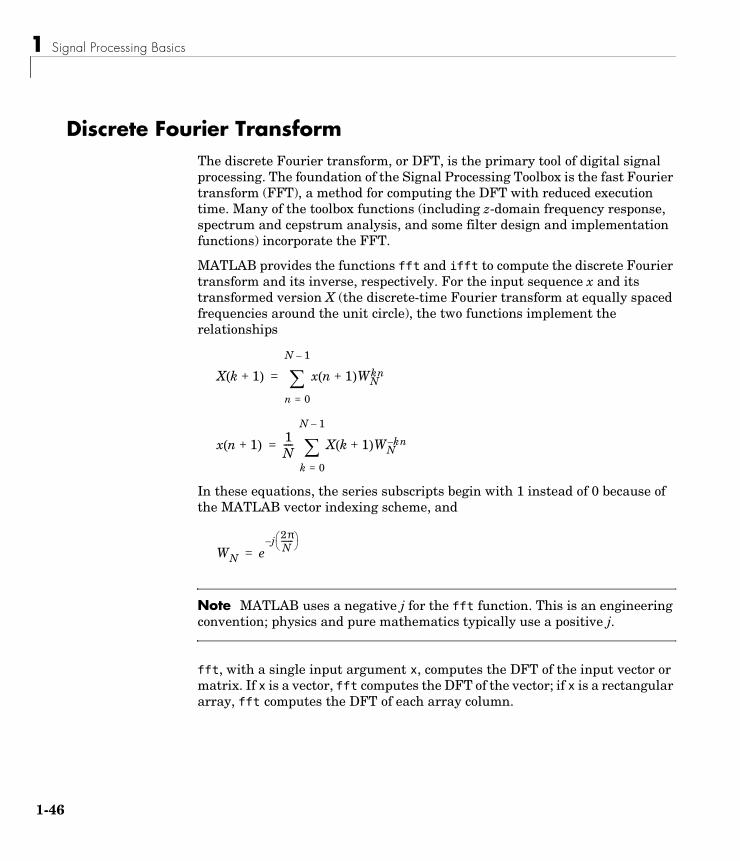
Discrete Fourier TransformThe discrete Fourier transform, or DFT, is the primary tool of digital signal processing. The foundation of the Signal Processing Toolbox is the fast Fourier transform (FFT), a method for computing the DFT with reduced execution time. Many of the toolbox functions (including z-domain frequency response, spectrum and cepstrum analysis, and some filter design and implementation functions) incorporate the FFT.
MATLAB provides the functions fft and ifft to compute the discrete Fourier transform and its inverse, respectively. For the input sequence x and its transformed version X (the discrete-time Fourier transform at equally spaced frequencies around the unit circle), the two functions implement the relationships
In these equations, the series subscripts begin with 1 instead of 0 because of the MATLAB vector indexing scheme, and
Note MATLAB uses a negative j for the fft function. This is an engineering convention; physics and pure mathematics typically use a positive j.
fft, with a single input argument x, computes the DFT of the input vector or matrix. If x is a vector, fft computes the DFT of the vector; if x is a rectangular array, fft computes the DFT of each array column.
X k 1+( ) x n 1+( )WNkn
n 0=
N 1–
∑=
x n 1+( )1N---- X k 1+( )WN
kn–
k 0=
N 1–
∑=
WN ej–
2πN-------
=
6
Discrete Fourier Transform
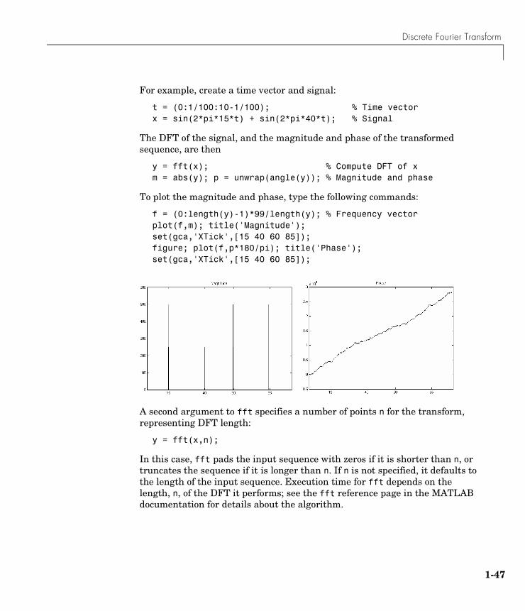
For example, create a time vector and signal:
t = (0:1/100:10-1/100); % Time vectorx = sin(2*pi*15*t) + sin(2*pi*40*t); % Signal
The DFT of the signal, and the magnitude and phase of the transformed sequence, are then
y = fft(x); % Compute DFT of xm = abs(y); p = unwrap(angle(y)); % Magnitude and phase
To plot the magnitude and phase, type the following commands:
f = (0:length(y)-1)*99/length(y); % Frequency vectorplot(f,m); title('Magnitude');set(gca,'XTick',[15 40 60 85]);figure; plot(f,p*180/pi); title('Phase');set(gca,'XTick',[15 40 60 85]);
A second argument to fft specifies a number of points n for the transform, representing DFT length:
y = fft(x,n);
In this case, fft pads the input sequence with zeros if it is shorter than n, or truncates the sequence if it is longer than n. If n is not specified, it defaults to the length of the input sequence. Execution time for fft depends on the length, n, of the DFT it performs; see the fft reference page in the MATLAB documentation for details about the algorithm.
1-47
1 Signal Processing Basics
1-4
Note The resulting FFT amplitude is A*n/2, where A is the original amplitude and n is the number of FFT points. This is true only if the number of FFT points is greater than or equal to the number of data samples. If the number of FFT points is less, the FFT amplitude is lower than the original amplitude by the above amount.
The inverse discrete Fourier transform function ifft also accepts an input sequence and, optionally, the number of desired points for the transform. Try the example below; the original sequence x and the reconstructed sequence are identical (within rounding error).
t = (0:1/255:1);x = sin(2*pi*120*t);y = real(ifft(fft(x)));
This toolbox also includes functions for the two-dimensional FFT and its inverse, fft2 and ifft2. These functions are useful for two-dimensional signal or image processing. The goertzel function, which is another algorithm to compute the DFT, also is included in the toolbox. This function is efficient for computing the DFT of a portion of a long signal.
It is sometimes convenient to rearrange the output of the fft or fft2 function so the zero frequency component is at the center of the sequence. The MATLAB function fftshift moves the zero frequency component to the center of a vector or matrix.
8

Selected Bibliography
Selected BibliographyAlgorithm development for the Signal Processing Toolbox has drawn heavily upon the references listed below. All are recommended to the interested reader who needs to know more about signal processing than is covered in this manual.
[1] Crochiere, R.E., and L.R. Rabiner. Multi-Rate Signal Processing. Englewood Cliffs, NJ: Prentice Hall, 1983. Pgs. 88-91.
[2] IEEE. Programs for Digital Signal Processing. IEEE Press. New York: John Wiley & Sons, 1979.
[3] Jackson, L.B. Digital Filters and Signal Processing. Third Ed. Boston: Kluwer Academic Publishers, 1989.
[4] Kay, S.M. Modern Spectral Estimation. Englewood Cliffs, NJ: Prentice Hall, 1988.
[5] Oppenheim, A.V., and R.W. Schafer. Discrete-Time Signal Processing. Englewood Cliffs, NJ: Prentice Hall, 1989.
[6] Parks, T.W., and C.S. Burrus. Digital Filter Design. New York: John Wiley & Sons, 1987.
[7] Percival, D.B., and A.T. Walden. Spectral Analysis for Physical Applications: Multitaper and Conventional Univariate Techniques. Cambridge: Cambridge University Press, 1993.
[8] Pratt,W.K. Digital Image Processing. New York: John Wiley & Sons, 1991.
[9] Proakis, J.G., and D.G. Manolakis. Digital Signal Processing: Principles, Algorithms, and Applications. Upper Saddle River, NJ: Prentice Hall, 1996.
[10] Rabiner, L.R., and B. Gold. Theory and Application of Digital Signal Processing. Englewood Cliffs, NJ: Prentice Hall, 1975.
[11] Welch, P.D. “The Use of Fast Fourier Transform for the Estimation of Power Spectra: A Method Based on Time Averaging Over Short, Modified Periodograms.” IEEE Trans. Audio Electroacoust. Vol. AU-15 (June 1967). Pgs. 70-73.
1-49

1 Signal Processing Basics
1-5
0
2
Filter Design and Implementation
Filter design is the process of creating the filter coefficients to meet specific filtering requirements. Filter implementation involves choosing and applying a particular filter structure to those coefficients. Only after both design and implementation have been performed can data be filtered. The following chapter describes filter design and implementation in the Signal Processing Toolbox.
Filter Requirements and Specification (p. 2-2)
Overview of filter design
IIR Filter Design (p. 2-4) Infinite impulse reponse filters (Butterworth, Chebyshev, elliptic, Bessel, Yule-Walker, and parametric methods)
FIR Filter Design (p. 2-17) Finite impulse reponse filters (windowing, multiband, least squares, nonlinear phase, complex filters, raised cosine)
Special Topics in IIR Filter Design (p. 2-44)
Analog design, frequency transformation, filter discretization
Filter Implementation (p. 2-53) Filtering with your filter
Selected Bibliography (p. 2-55) Sources for additional information
2 Filter Design and Implementation
2-2
Filter Requirements and SpecificationThe goal of filter design is to perform frequency dependent alteration of a data sequence. A possible requirement might be to remove noise above 30 Hz from a data sequence sampled at 100 Hz. A more rigorous specification might call for a specific amount of passband ripple, stopband attenuation, or transition width. A very precise specification could ask to achieve the performance goals with the minimum filter order, or it could call for an arbitrary magnitude shape, or it might require an FIR filter.
Filter design methods differ primarily in how performance is specified. For “loosely specified” requirements, as in the first case above, a Butterworth IIR filter is often sufficient. To design a fifth-order 30 Hz lowpass Butterworth filter and apply it to the data in vector x:
[b,a] = butter(5,30/50);Hd = dfilt.df2t(b,a); %Direct-form II transposed structurey = filter(Hd,x);
The second input argument to butter specifies the cutoff frequency, normalized to half the sampling frequency (the Nyquist frequency).
All of the filter design functions operate with normalized frequencies, so they do not require the system sampling rate as an extra input argument. This toolbox uses the convention that unit frequency is the Nyquist frequency, defined as half the sampling frequency. The normalized frequency, therefore, is always in the interval 0 ≤ f ≤ 1. For a system with a 1000 Hz sampling frequency, 300 Hz is 300/500 = 0.6. To convert normalized frequency to angular frequency around the unit circle, multiply by π. To convert normalized frequency back to hertz, multiply by half the sample frequency.
More rigorous filter requirements traditionally include passband ripple (Rp, in decibels), stopband attenuation (Rs, in decibels), and transition width (Ws-Wp, in hertz).
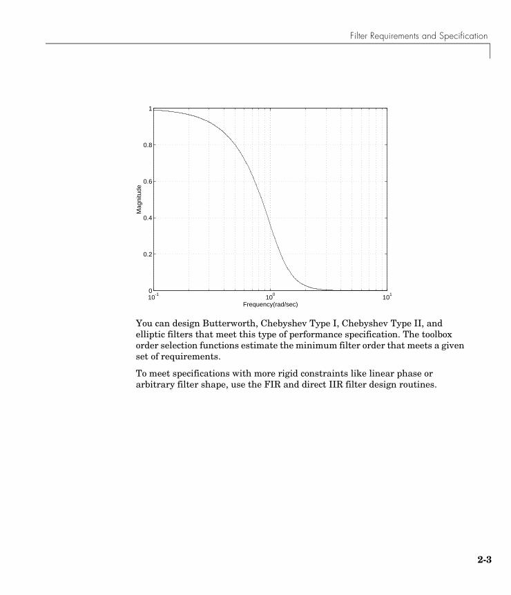
Filter Requirements and Specification
You can design Butterworth, Chebyshev Type I, Chebyshev Type II, and elliptic filters that meet this type of performance specification. The toolbox order selection functions estimate the minimum filter order that meets a given set of requirements.
To meet specifications with more rigid constraints like linear phase or arbitrary filter shape, use the FIR and direct IIR filter design routines.
10-1
100
101
0
0.2
0.4
0.6
0.8
1
Frequency(rad/sec)
Mag
nitu
de
2-3
2 Filter Design and Implementation
2-4
IIR Filter DesignThe primary advantage of IIR filters over FIR filters is that they typically meet a given set of specifications with a much lower filter order than a corresponding FIR filter. Although IIR filters have nonlinear phase, data processing within MATLAB is commonly performed “off-line,” that is, the entire data sequence is available prior to filtering. This allows for a noncausal, zero-phase filtering approach (via the filtfilt function), which eliminates the nonlinear phase distortion of an IIR filter.
The classical IIR filters, Butterworth, Chebyshev Types I and II, elliptic, and Bessel, all approximate the ideal “brick wall” filter in different ways. This toolbox provides functions to create all these types of classical IIR filters in both the analog and digital domains (except Bessel, for which only the analog case is supported), and in lowpass, highpass, bandpass, and bandstop configurations. For most filter types, you can also find the lowest filter order that fits a given filter specification in terms of passband and stopband attenuation, and transition width(s).
The direct filter design function yulewalk finds a filter with magnitude response approximating a desired function. This is one way to create a multiband bandpass filter.
You can also use the parametric modeling or system identification functions to design IIR filters. These functions are discussed in “Parametric Modeling” on page 4-17.
The generalized Butterworth design function maxflat is discussed in the section “Generalized Butterworth Filter Design” on page 2-15.
The following table summarizes the various filter methods in the toolbox and lists the functions available to implement these methods.
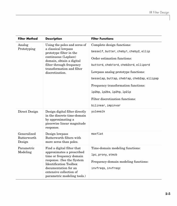
IIR Filter Design
Filter Method Description Filter Functions
Analog Prototyping
Using the poles and zeros of a classical lowpass prototype filter in the continuous (Laplace) domain, obtain a digital filter through frequency transformation and filter discretization.
Complete design functions:
besself, butter, cheby1, cheby2, ellip
Order estimation functions:
buttord, cheb1ord, cheb2ord, ellipord
Lowpass analog prototype functions:
besselap, buttap, cheb1ap, cheb2ap, ellipap
Frequency transformation functions:
lp2bp, lp2bs, lp2hp, lp2lp
Filter discretization functions:
bilinear, impinvar
Direct Design Design digital filter directly in the discrete time-domain by approximating a piecewise linear magnitude response.
yulewalk
Generalized Butterworth Design
Design lowpass Butterworth filters with more zeros than poles.
maxflat
Parametric Modeling
Find a digital filter that approximates a prescribed time or frequency domain response. (See the System Identification Toolbox documentation for an extensive collection of parametric modeling tools.)
Time-domain modeling functions:
lpc, prony, stmcb
Frequency-domain modeling functions:
invfreqs, invfreqz
2-5
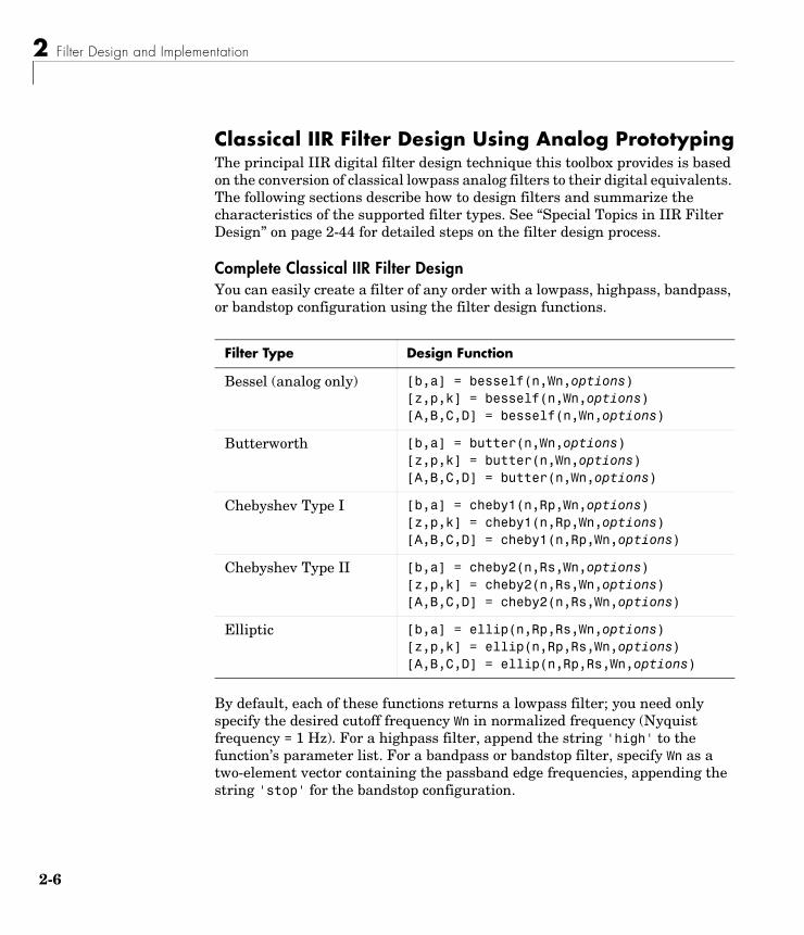
2 Filter Design and Implementation
2-6
Classical IIR Filter Design Using Analog PrototypingThe principal IIR digital filter design technique this toolbox provides is based on the conversion of classical lowpass analog filters to their digital equivalents. The following sections describe how to design filters and summarize the characteristics of the supported filter types. See “Special Topics in IIR Filter Design” on page 2-44 for detailed steps on the filter design process.
Complete Classical IIR Filter DesignYou can easily create a filter of any order with a lowpass, highpass, bandpass, or bandstop configuration using the filter design functions.
By default, each of these functions returns a lowpass filter; you need only specify the desired cutoff frequency Wn in normalized frequency (Nyquist frequency = 1 Hz). For a highpass filter, append the string 'high' to the function’s parameter list. For a bandpass or bandstop filter, specify Wn as a two-element vector containing the passband edge frequencies, appending the string 'stop' for the bandstop configuration.
Filter Type Design Function
Bessel (analog only) [b,a] = besself(n,Wn,options)[z,p,k] = besself(n,Wn,options)[A,B,C,D] = besself(n,Wn,options)
Butterworth [b,a] = butter(n,Wn,options)[z,p,k] = butter(n,Wn,options)[A,B,C,D] = butter(n,Wn,options)
Chebyshev Type I [b,a] = cheby1(n,Rp,Wn,options)[z,p,k] = cheby1(n,Rp,Wn,options)[A,B,C,D] = cheby1(n,Rp,Wn,options)
Chebyshev Type II [b,a] = cheby2(n,Rs,Wn,options)[z,p,k] = cheby2(n,Rs,Wn,options)[A,B,C,D] = cheby2(n,Rs,Wn,options)
Elliptic [b,a] = ellip(n,Rp,Rs,Wn,options)[z,p,k] = ellip(n,Rp,Rs,Wn,options)[A,B,C,D] = ellip(n,Rp,Rs,Wn,options)
IIR Filter Design
Here are some example digital filters:
[b,a] = butter(5,0.4); % Lowpass Butterworth[b,a] = cheby1(4,1,[0.4 0.7]); % Bandpass Chebyshev Type I[b,a] = cheby2(6,60,0.8,'high'); % Highpass Chebyshev Type II[b,a] = ellip(3,1,60,[0.4 0.7],'stop'); % Bandstop elliptic
To design an analog filter, perhaps for simulation, use a trailing 's' and specify cutoff frequencies in rad/s:
[b,a] = butter(5,.4,'s'); % Analog Butterworth filter
All filter design functions return a filter in the transfer function, zero-pole-gain, or state-space linear system model representation, depending on how many output arguments are present.
Note All classical IIR lowpass filters are ill-conditioned for extremely low cut-off frequencies. Therefore, instead of designing a lowpass IIR filter with a very narrow passband, it can be better to design a wider passband and decimate the input signal.
Designing IIR Filters to Frequency Domain SpecificationsThis toolbox provides order selection functions that calculate the minimum filter order that meets a given set of requirements.
These are useful in conjunction with the filter design functions. Suppose you want a bandpass filter with a passband from 1000 to 2000 Hz, stopbands starting 500 Hz away on either side, a 10 kHz sampling frequency, at most 1 dB
Filter Type Order Estimation Function
Butterworth [n,Wn] = buttord(Wp,Ws,Rp,Rs)
Chebyshev Type I [n,Wn] = cheb1ord(Wp, Ws, Rp, Rs)
Chebyshev Type II [n,Wn] = cheb2ord(Wp, Ws, Rp, Rs)
Elliptic [n,Wn] = ellipord(Wp, Ws, Rp, Rs)
2-7
2 Filter Design and Implementation
2-8
of passband ripple, and at least 60 dB of stopband attenuation. You can meet these specifications by using the butter function as follows.
[n,Wn] = buttord([1000 2000]/5000,[500 2500]/5000,1,60)
n = 12Wn = 0.1951 0.4080
[b,a] = butter(n,Wn);
An elliptic filter that meets the same requirements is given by
[n,Wn] = ellipord([1000 2000]/5000,[500 2500]/5000,1,60)
n = 5Wn = 0.2000 0.4000
[b,a] = ellip(n,1,60,Wn);
These functions also work with the other standard band configurations, as well as for analog filters.
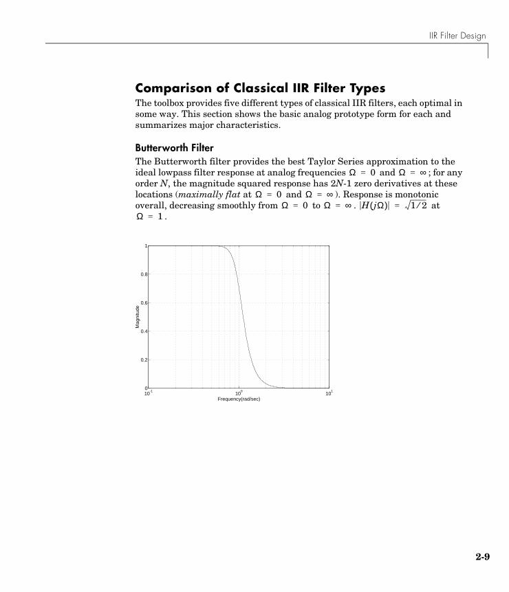
IIR Filter Design
Comparison of Classical IIR Filter TypesThe toolbox provides five different types of classical IIR filters, each optimal in some way. This section shows the basic analog prototype form for each and summarizes major characteristics.
Butterworth FilterThe Butterworth filter provides the best Taylor Series approximation to the ideal lowpass filter response at analog frequencies and ; for any order N, the magnitude squared response has 2N-1 zero derivatives at these locations (maximally flat at and ). Response is monotonic overall, decreasing smoothly from to . at
.
Ω 0= Ω ∞=
Ω 0= Ω ∞=Ω 0= Ω ∞= H jΩ( ) 1 2⁄=
Ω 1=
10-1
100
101
0
0.2
0.4
0.6
0.8
1
Frequency(rad/sec)
Mag
nitu
de
2-9
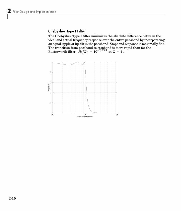
2 Filter Design and Implementation
2-1
Chebyshev Type I FilterThe Chebyshev Type I filter minimizes the absolute difference between the ideal and actual frequency response over the entire passband by incorporating an equal ripple of Rp dB in the passband. Stopband response is maximally flat. The transition from passband to stopband is more rapid than for the Butterworth filter. at .H jΩ( ) 10 Rp 20⁄–
= Ω 1=
10-1
100
101
0
0.2
0.4
0.6
0.8
1
Frequency(rad/sec)
Mag
nitu
de
0
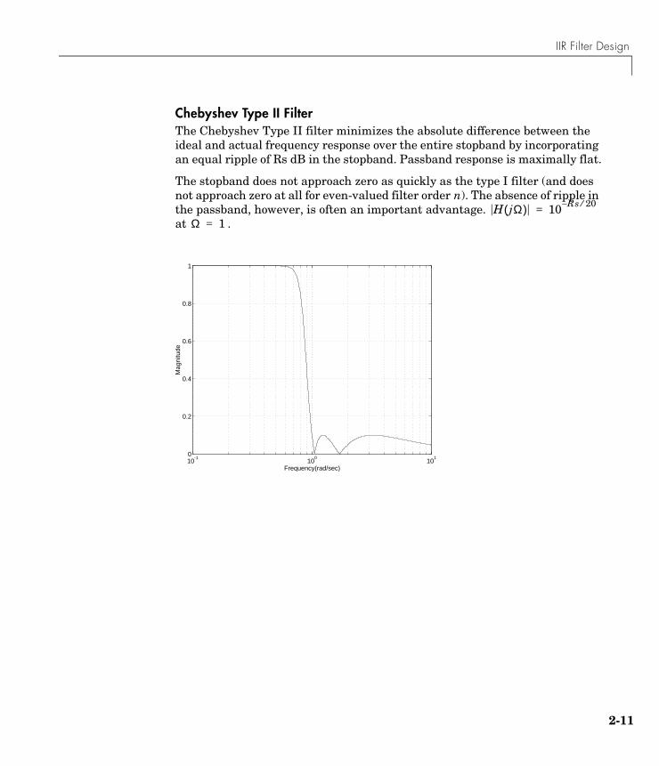
IIR Filter Design
Chebyshev Type II FilterThe Chebyshev Type II filter minimizes the absolute difference between the ideal and actual frequency response over the entire stopband by incorporating an equal ripple of Rs dB in the stopband. Passband response is maximally flat.
The stopband does not approach zero as quickly as the type I filter (and does not approach zero at all for even-valued filter order n). The absence of ripple in the passband, however, is often an important advantage. at .
H jΩ( ) 10 Rs 20⁄–=
Ω 1=
10-1
100
101
0
0.2
0.4
0.6
0.8
1
Frequency(rad/sec)
Mag
nitu
de
2-11
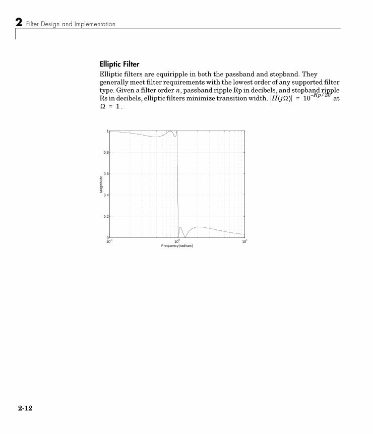
2 Filter Design and Implementation
2-1
Elliptic FilterElliptic filters are equiripple in both the passband and stopband. They generally meet filter requirements with the lowest order of any supported filter type. Given a filter order n, passband ripple Rp in decibels, and stopband ripple Rs in decibels, elliptic filters minimize transition width. at
.H jΩ( ) 10 Rp 20⁄–
=Ω 1=
10-1
100
101
0
0.2
0.4
0.6
0.8
1
Frequency(rad/sec)
Mag
nitu
de
2
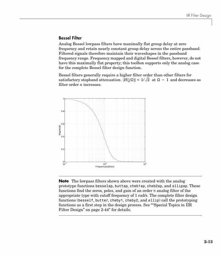
IIR Filter Design
Bessel FilterAnalog Bessel lowpass filters have maximally flat group delay at zero frequency and retain nearly constant group delay across the entire passband. Filtered signals therefore maintain their waveshapes in the passband frequency range. Frequency mapped and digital Bessel filters, however, do not have this maximally flat property; this toolbox supports only the analog case for the complete Bessel filter design function.
Bessel filters generally require a higher filter order than other filters for satisfactory stopband attenuation. at and decreases as filter order n increases.
Note The lowpass filters shown above were created with the analog prototype functions besselap, buttap, cheb1ap, cheb2ap, and ellipap. These functions find the zeros, poles, and gain of an order n analog filter of the appropriate type with cutoff frequency of 1 rad/s. The complete filter design functions (besself, butter, cheby1, cheby2, and ellip) call the prototyping functions as a first step in the design process. See ““Special Topics in IIR Filter Design” on page 2-44” for details.
H jΩ( ) 1 2⁄< Ω 1=
10-1
100
101
0
0.2
0.4
0.6
0.8
1
Frequency(rad/sec)
Mag
nitu
de
2-13
2 Filter Design and Implementation
2-1
To create similar plots, use n = 5 and, as needed, Rp = 0.5 and Rs = 20. For example, to create the elliptic filter plot:
[z,p,k] = ellipap(5,0.5,20);w = logspace(-1,1,1000);h = freqs(k*poly(z),poly(p),w);semilogx(w,abs(h)), grid
Direct IIR Filter DesignThis toolbox uses the term direct methods to describe techniques for IIR design that find a filter based on specifications in the discrete domain. Unlike the analog prototyping method, direct design methods are not constrained to the standard lowpass, highpass, bandpass, or bandstop configurations. Rather, these functions design filters with an arbitrary, perhaps multiband, frequency response. This section discusses the yulewalk function, which is intended specifically for filter design; “Parametric Modeling” on page 4-17 discusses other methods that may also be considered direct, such as Prony’s method, Linear Prediction, the Steiglitz-McBride method, and inverse frequency design.
The yulewalk function designs recursive IIR digital filters by fitting a specified frequency response. yulewalk’s name reflects its method for finding the filter’s denominator coefficients: it finds the inverse FFT of the ideal desired power spectrum and solves the “modified Yule-Walker equations” using the resulting autocorrelation function samples. The statement
[b,a] = yulewalk(n,f,m)
returns row vectors b and a containing the n+1 numerator and denominator coefficients of the order n IIR filter whose frequency-magnitude characteristics approximate those given in vectors f and m. f is a vector of frequency points ranging from 0 to 1, where 1 represents the Nyquist frequency. m is a vector containing the desired magnitude response at the points in f. f and m can describe any piecewise linear shape magnitude response, including a multiband response. The FIR counterpart of this function is fir2, which also designs a filter based on an arbitrary piecewise linear magnitude response. See ““FIR Filter Design” on page 2-17” for details.
Note that yulewalk does not accept phase information, and no statements are made about the optimality of the resulting filter.
4
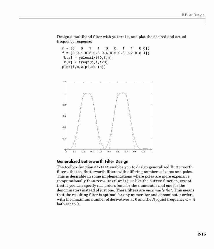
IIR Filter Design
Design a multiband filter with yulewalk, and plot the desired and actual frequency response:
m = [0 0 1 1 0 0 1 1 0 0];f = [0 0.1 0.2 0.3 0.4 0.5 0.6 0.7 0.8 1];[b,a] = yulewalk(10,f,m);[h,w] = freqz(b,a,128)plot(f,m,w/pi,abs(h))
Generalized Butterworth Filter DesignThe toolbox function maxflat enables you to design generalized Butterworth filters, that is, Butterworth filters with differing numbers of zeros and poles. This is desirable in some implementations where poles are more expensive computationally than zeros. maxflat is just like the butter function, except that it you can specify two orders (one for the numerator and one for the denominator) instead of just one. These filters are maximally flat. This means that the resulting filter is optimal for any numerator and denominator orders, with the maximum number of derivatives at 0 and the Nyquist frequency ω = π both set to 0.
0 0.1 0.2 0.3 0.4 0.5 0.6 0.7 0.8 0.9 10
0.2
0.4
0.6
0.8
1
1.2
2-15
2 Filter Design and Implementation
2-1
For example, when the two orders are the same, maxflat is the same as butter:
[b,a] = maxflat(3,3,0.25)
b = 0.0317 0.0951 0.0951 0.0317
a = 1.0000 -1.4590 0.9104 -0.1978
[b,a] = butter(3,0.25)
b = 0.0317 0.0951 0.0951 0.0317
a = 1.0000 -1.4590 0.9104 -0.1978
However, maxflat is more versatile because it allows you to design a filter with more zeros than poles:
[b,a] = maxflat(3,1,0.25)
b = 0.0950 0.2849 0.2849 0.0950
a = 1.0000 -0.2402
The third input to maxflat is the half-power frequency, a frequency between 0 and 1 with a desired magnitude response of .
You can also design linear phase filters that have the maximally flat property using the 'sym' option:
maxflat(4,'sym',0.3)
ans = 0.0331 0.2500 0.4337 0.2500 0.0331
For complete details of the maxflat algorithm, see Selesnick and Burrus [2].
1 2⁄
6
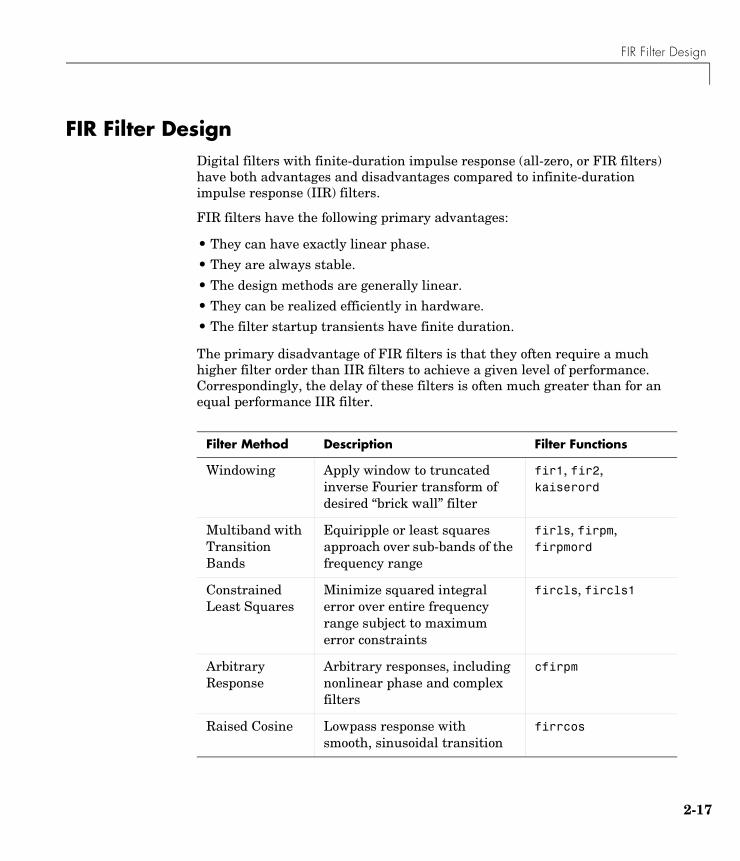
FIR Filter Design
FIR Filter DesignDigital filters with finite-duration impulse response (all-zero, or FIR filters) have both advantages and disadvantages compared to infinite-duration impulse response (IIR) filters.
FIR filters have the following primary advantages:
• They can have exactly linear phase.
• They are always stable.
• The design methods are generally linear.
• They can be realized efficiently in hardware.
• The filter startup transients have finite duration.
The primary disadvantage of FIR filters is that they often require a much higher filter order than IIR filters to achieve a given level of performance. Correspondingly, the delay of these filters is often much greater than for an equal performance IIR filter.
Filter Method Description Filter Functions
Windowing Apply window to truncated inverse Fourier transform of desired “brick wall” filter
fir1, fir2, kaiserord
Multiband with Transition Bands
Equiripple or least squares approach over sub-bands of the frequency range
firls, firpm, firpmord
Constrained Least Squares
Minimize squared integral error over entire frequency range subject to maximum error constraints
fircls, fircls1
Arbitrary Response
Arbitrary responses, including nonlinear phase and complex filters
cfirpm
Raised Cosine Lowpass response with smooth, sinusoidal transition
firrcos
2-17
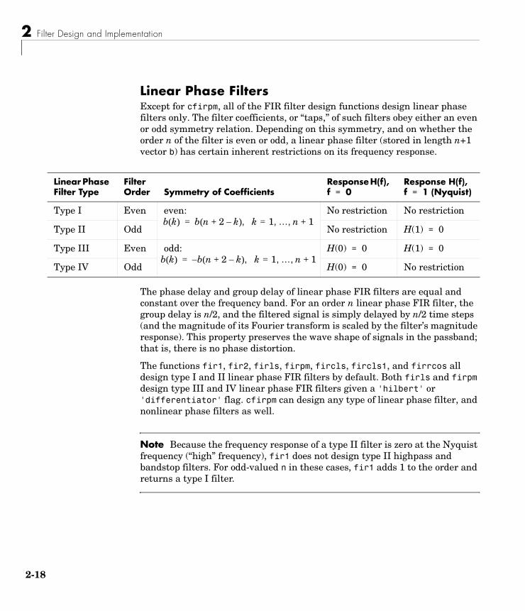
2 Filter Design and Implementation
2-1
Linear Phase FiltersExcept for cfirpm, all of the FIR filter design functions design linear phase filters only. The filter coefficients, or “taps,” of such filters obey either an even or odd symmetry relation. Depending on this symmetry, and on whether the order n of the filter is even or odd, a linear phase filter (stored in length n+1 vector b) has certain inherent restrictions on its frequency response.
The phase delay and group delay of linear phase FIR filters are equal and constant over the frequency band. For an order n linear phase FIR filter, the group delay is n/2, and the filtered signal is simply delayed by n/2 time steps (and the magnitude of its Fourier transform is scaled by the filter’s magnitude response). This property preserves the wave shape of signals in the passband; that is, there is no phase distortion.
The functions fir1, fir2, firls, firpm, fircls, fircls1, and firrcos all design type I and II linear phase FIR filters by default. Both firls and firpm design type III and IV linear phase FIR filters given a 'hilbert' or 'differentiator' flag. cfirpm can design any type of linear phase filter, and nonlinear phase filters as well.
Note Because the frequency response of a type II filter is zero at the Nyquist frequency (“high” frequency), fir1 does not design type II highpass and bandstop filters. For odd-valued n in these cases, fir1 adds 1 to the order and returns a type I filter.
Linear Phase Filter Type
Filter Order Symmetry of Coefficients
Response H(f), f = 0
Response H(f), f = 1 (Nyquist)
Type I Even even: No restriction No restriction
Type II Odd No restriction H(1) = 0
Type III Even odd: H(0) = 0 H(1) = 0
Type IV Odd H(0) = 0 No restriction
b k( ) b n 2 k–+( ) k 1= … n 1+, , ,=
b k( ) b– n 2 k–+( ) k 1= … n 1+, , ,=
8
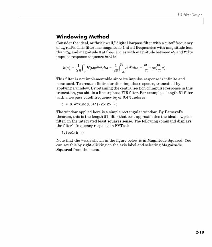
FIR Filter Design
Windowing MethodConsider the ideal, or “brick wall,” digital lowpass filter with a cutoff frequency of ω0 rad/s. This filter has magnitude 1 at all frequencies with magnitude less than ω0, and magnitude 0 at frequencies with magnitude between ω0 and π. Its impulse response sequence h(n) is
This filter is not implementable since its impulse response is infinite and noncausal. To create a finite-duration impulse response, truncate it by applying a window. By retaining the central section of impulse response in this truncation, you obtain a linear phase FIR filter. For example, a length 51 filter with a lowpass cutoff frequency ω0 of rad/s is
b = 0.4*sinc(0.4*(-25:25));
The window applied here is a simple rectangular window. By Parseval’s theorem, this is the length 51 filter that best approximates the ideal lowpass filter, in the integrated least squares sense. The following command displays the filter’s frequency response in FVTool:
fvtool(b,1)
Note that the y-axis shown in the figure below is in Magnitude Squared. You can set this by right-clicking on the axis label and selecting Magnitude Squared from the menu.
h n( )1
2π------ H ω( )ejωn ωd
π–
π
∫1
2π------ ejωn ωd
ω0–
ω0
∫ω0π
-------sincω0π
-------n( )= = =
0.4π
2-19
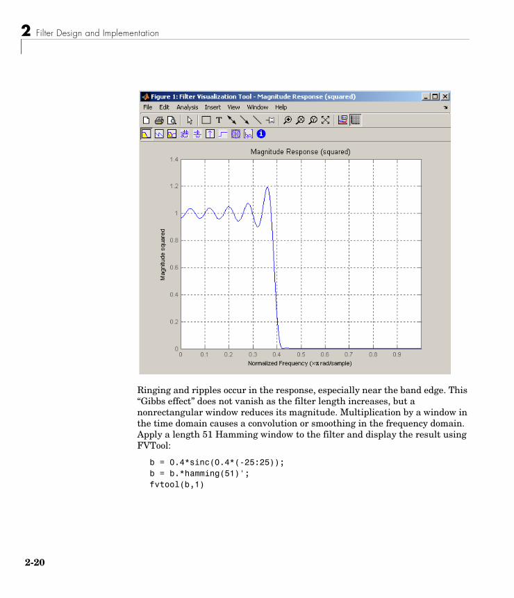
2 Filter Design and Implementation
2-2
Ringing and ripples occur in the response, especially near the band edge. This “Gibbs effect” does not vanish as the filter length increases, but a nonrectangular window reduces its magnitude. Multiplication by a window in the time domain causes a convolution or smoothing in the frequency domain. Apply a length 51 Hamming window to the filter and display the result using FVTool:
b = 0.4*sinc(0.4*(-25:25));b = b.*hamming(51)';fvtool(b,1)
0
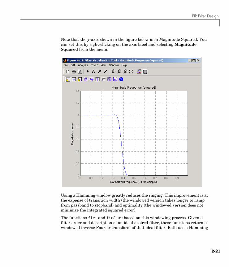
FIR Filter Design
Note that the y-axis shown in the figure below is in Magnitude Squared. You can set this by right-clicking on the axis label and selecting Magnitude Squared from the menu.
Using a Hamming window greatly reduces the ringing. This improvement is at the expense of transition width (the windowed version takes longer to ramp from passband to stopband) and optimality (the windowed version does not minimize the integrated squared error).
The functions fir1 and fir2 are based on this windowing process. Given a filter order and description of an ideal desired filter, these functions return a windowed inverse Fourier transform of that ideal filter. Both use a Hamming
2-21
2 Filter Design and Implementation
2-2
window by default, but they accept any window function. See the “Windows” on page 4-2 for an overview of windows and their properties.
Standard Band FIR Filter Design: fir1fir1 implements the classical method of windowed linear phase FIR digital filter design. It resembles the IIR filter design functions in that it is formulated to design filters in standard band configurations: lowpass, bandpass, highpass, and bandstop.
The statements
n = 50;Wn = 0.4;b = fir1(n,Wn);
create row vector b containing the coefficients of the order n Hamming-windowed filter. This is a lowpass, linear phase FIR filter with cutoff frequency Wn. Wn is a number between 0 and 1, where 1 corresponds to the Nyquist frequency, half the sampling frequency. (Unlike other methods, here Wn corresponds to the 6 dB point.) For a highpass filter, simply append the string 'high' to the function’s parameter list. For a bandpass or bandstop filter, specify Wn as a two-element vector containing the passband edge frequencies; append the string 'stop' for the bandstop configuration.
b = fir1(n,Wn,window) uses the window specified in column vector window for the design. The vector window must be n+1 elements long. If you do not specify a window, fir1 applies a Hamming window.
Kaiser Window Order Estimation. The kaiserord function estimates the filter order, cutoff frequency, and Kaiser window beta parameter needed to meet a given set of specifications. Given a vector of frequency band edges and a corresponding vector of magnitudes, as well as maximum allowable ripple, kaiserord returns appropriate input parameters for the fir1 function.
Multiband FIR Filter Design: fir2The fir2 function also designs windowed FIR filters, but with an arbitrarily shaped piecewise linear frequency response. This is in contrast to fir1, which only designs filters in standard lowpass, highpass, bandpass, and bandstop configurations.
2
FIR Filter Design
The commands
n = 50;f = [0 .4 .5 1];m = [1 1 0 0];b = fir2(n,f,m);
return row vector b containing the n+1 coefficients of the order n FIR filter whose frequency-magnitude characteristics match those given by vectors f and m. f is a vector of frequency points ranging from 0 to 1, where 1 represents the Nyquist frequency. m is a vector containing the desired magnitude response at the points specified in f. (The IIR counterpart of this function is yulewalk, which also designs filters based on arbitrary piecewise linear magnitude responses. See “IIR Filter Design” on page 2-4 for details.)
Multiband FIR Filter Design with Transition BandsThe firls and firpm functions provide a more general means of specifying the ideal desired filter than the fir1 and fir2 functions. These functions design Hilbert transformers, differentiators, and other filters with odd symmetric coefficients (type III and type IV linear phase). They also let you include transition or “don’t care” regions in which the error is not minimized, and perform band dependent weighting of the minimization.
The firls function is an extension of the fir1 and fir2 functions in that it minimizes the integral of the square of the error between the desired frequency response and the actual frequency response.
The firpm function implements the Parks-McClellan algorithm, which uses the Remez exchange algorithm and Chebyshev approximation theory to design filters with optimal fits between the desired and actual frequency responses. The filters are optimal in the sense that they minimize the maximum error between the desired frequency response and the actual frequency response; they are sometimes called minimax filters. Filters designed in this way exhibit an equiripple behavior in their frequency response, and hence are also known as equiripple filters. The Parks-McClellan FIR filter design algorithm is perhaps the most popular and widely used FIR filter design methodology.
The syntax for firls and firpm is the same; the only difference is their minimization schemes. The next example shows how filters designed with firls and firpm reflect these different schemes.
2-23
2 Filter Design and Implementation
2-2
Basic ConfigurationsThe default mode of operation of firls and firpm is to design type I or type II linear phase filters, depending on whether the order you desire is even or odd, respectively. A lowpass example with approximate amplitude 1 from 0 to 0.4 Hz, and approximate amplitude 0 from 0.5 to 1.0 Hz is
n = 20; % Filter orderf = [0 0.4 0.5 1]; % Frequency band edgesa = [1 1 0 0]; % Desired amplitudesb = firpm(n,f,a);
From 0.4 to 0.5 Hz, firpm performs no error minimization; this is a transition band or “don’t care” region. A transition band minimizes the error more in the bands that you do care about, at the expense of a slower transition rate. In this way, these types of filters have an inherent trade-off similar to FIR design by windowing.
To compare least squares to equiripple filter design, use firls to create a similar filter. Type
bb = firls(n,f,a);
and compare their frequency responses using FVTool:
fvtool(b,1,bb,1)
Note that the y-axis shown in the figure below is in Magnitude Squared. You can set this by right-clicking on the axis label and selecting Magnitude Squared from the menu.
4
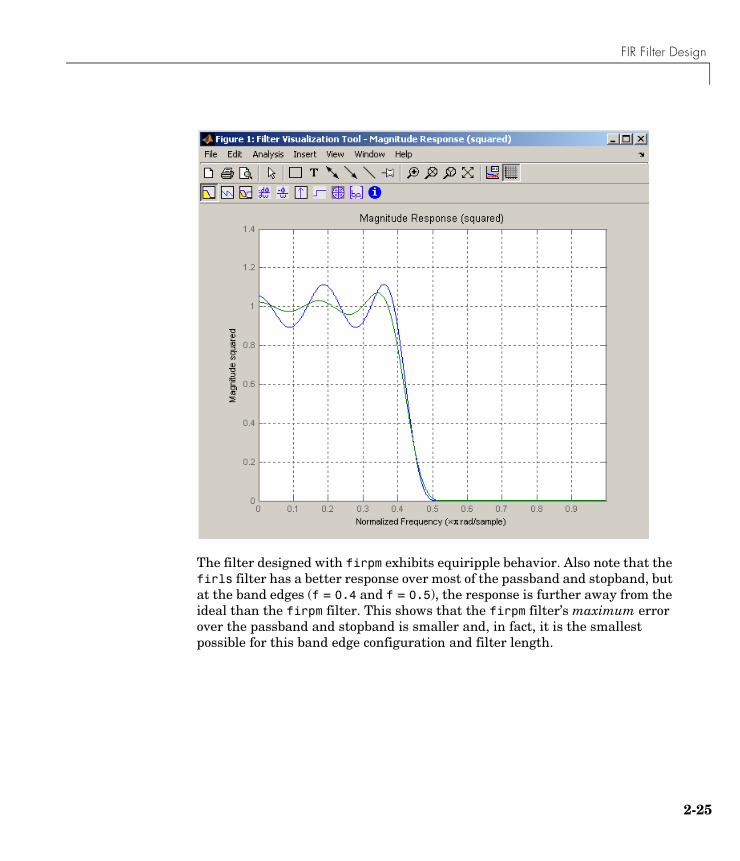
FIR Filter Design
The filter designed with firpm exhibits equiripple behavior. Also note that the firls filter has a better response over most of the passband and stopband, but at the band edges (f = 0.4 and f = 0.5), the response is further away from the ideal than the firpm filter. This shows that the firpm filter’s maximum error over the passband and stopband is smaller and, in fact, it is the smallest possible for this band edge configuration and filter length.
2-25
2 Filter Design and Implementation
2-2
Think of frequency bands as lines over short frequency intervals. firpm and firls use this scheme to represent any piecewise linear desired function with any transition bands. firls and firpm design lowpass, highpass, bandpass, and bandstop filters; a bandpass example is
f = [0 0.3 0.4 0.7 0.8 1]; % Band edges in pairsa = [0 0 1 1 0 0]; % Bandpass filter amplitude
Technically, these f and a vectors define five bands:
• Two stopbands, from 0.0 to 0.3 and from 0.8 to 1.0
• A passband from 0.4 to 0.7
• Two transition bands, from 0.3 to 0.4 and from 0.7 to 0.8
Example highpass and bandstop filters are
f = [0 0.7 0.8 1]; % Band edges in pairsa = [0 0 1 1]; % Highpass filter amplitude
f = [0 0.3 0.4 0.5 0.8 1]; % Band edges in pairsa = [1 1 0 0 1 1]; % Bandstop filter amplitude
An example multiband bandpass filter is
f = [0 0.1 0.15 0.25 0.3 0.4 0.45 0.55 0.6 0.7 0.75 0.85 0.9 1];a = [1 1 0 0 1 1 0 0 1 1 0 0 1 1];
Another possibility is a filter that has as a transition region the line connecting the passband with the stopband; this can help control “runaway” magnitude response in wide transition regions:
f = [0 0.4 0.42 0.48 0.5 1];a = [1 1 0.8 0.2 0 0]; % Passband,linear transition,stopband
6
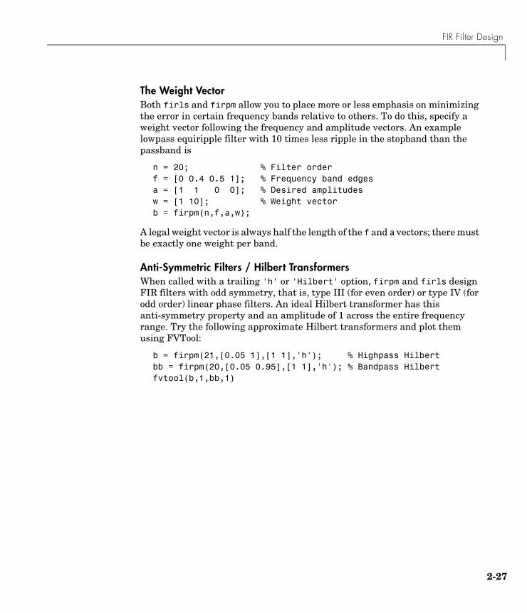
FIR Filter Design
The Weight VectorBoth firls and firpm allow you to place more or less emphasis on minimizing the error in certain frequency bands relative to others. To do this, specify a weight vector following the frequency and amplitude vectors. An example lowpass equiripple filter with 10 times less ripple in the stopband than the passband is
n = 20; % Filter orderf = [0 0.4 0.5 1]; % Frequency band edgesa = [1 1 0 0]; % Desired amplitudesw = [1 10]; % Weight vectorb = firpm(n,f,a,w);
A legal weight vector is always half the length of the f and a vectors; there must be exactly one weight per band.
Anti-Symmetric Filters / Hilbert TransformersWhen called with a trailing 'h' or 'Hilbert' option, firpm and firls design FIR filters with odd symmetry, that is, type III (for even order) or type IV (for odd order) linear phase filters. An ideal Hilbert transformer has this anti-symmetry property and an amplitude of 1 across the entire frequency range. Try the following approximate Hilbert transformers and plot them using FVTool:
b = firpm(21,[0.05 1],[1 1],'h'); % Highpass Hilbertbb = firpm(20,[0.05 0.95],[1 1],'h'); % Bandpass Hilbertfvtool(b,1,bb,1)
2-27
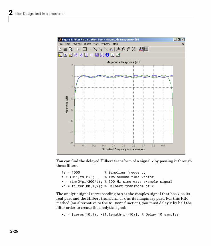
2 Filter Design and Implementation
2-2
You can find the delayed Hilbert transform of a signal x by passing it through these filters.
fs = 1000; % Sampling frequencyt = (0:1/fs:2)'; % Two second time vectorx = sin(2*pi*300*t); % 300 Hz sine wave example signalxh = filter(bb,1,x); % Hilbert transform of x
The analytic signal corresponding to x is the complex signal that has x as its real part and the Hilbert transform of x as its imaginary part. For this FIR method (an alternative to the hilbert function), you must delay x by half the filter order to create the analytic signal:
xd = [zeros(10,1); x(1:length(x)-10)]; % Delay 10 samples
8
FIR Filter Design
xa = xd + j*xh; % Analytic signal
This method does not work directly for filters of odd order, which require a noninteger delay. In this case, the hilbert function, described in “Specialized Transforms” on page 4-43, estimates the analytic signal. Alternatively, use the resample function to delay the signal by a noninteger number of samples.
DifferentiatorsDifferentiation of a signal in the time domain is equivalent to multiplication of the signal’s Fourier transform by an imaginary ramp function. That is, to differentiate a signal, pass it through a filter that has a response H(ω) = jω. Approximate the ideal differentiator (with a delay) using firpm or firls with a 'd' or 'differentiator' option:
b = firpm(21,[0 1],[0 pi*fs],'d');
To obtain the correct derivative, scale by pi*fs rad/s, where fs is the sampling frequency in hertz. For a type III filter, the differentiation band should stop short of the Nyquist frequency, and the amplitude vector must reflect that change to ensure the correct slope:
bb = firpm(20,[0 0.9],[0 0.9*pi*fs],'d');
In the 'd' mode, firpm weights the error by 1/ω in nonzero amplitude bands to minimize the maximum relative error. firls weights the error by (1/ω)2 in nonzero amplitude bands in the 'd' mode.
2-29
2 Filter Design and Implementation
2-3
The following plots show the magnitude responses for the differentiators above.
fvtool(b,1,bb,1)
0
FIR Filter Design
Constrained Least Squares FIR Filter DesignThe Constrained Least Squares (CLS) FIR filter design functions implement a technique that enables you to design FIR filters without explicitly defining the transition bands for the magnitude response. The ability to omit the specification of transition bands is useful in several situations. For example, it may not be clear where a rigidly defined transition band should appear if noise and signal information appear together in the same frequency band. Similarly, it may make sense to omit the specification of transition bands if they appear only to control the results of Gibbs phenomena that appear in the filter’s response. See Selesnick, Lang, and Burrus [2] for discussion of this method.
Instead of defining passbands, stopbands, and transition regions, the CLS method accepts a cutoff frequency (for the highpass, lowpass, bandpass, or bandstop cases), or passband and stopband edges (for multiband cases), for the desired response. In this way, the CLS method defines transition regions implicitly, rather than explicitly.
The key feature of the CLS method is that it enables you to define upper and lower thresholds that contain the maximum allowable ripple in the magnitude response. Given this constraint, the technique applies the least square error minimization technique over the frequency range of the filter’s response, instead of over specific bands. The error minimization includes any areas of discontinuity in the ideal, “brick wall” response. An additional benefit is that the technique enables you to specify arbitrarily small peaks resulting from Gibbs’ phenomena.
There are two toolbox functions that implement this design technique.
For details on the calling syntax for these functions, see their reference descriptions in the Function Reference.
Description Function
Constrained least square multiband FIR filter design fircls
Constrained least square filter design for lowpass and highpass linear phase filters
fircls1
2-31
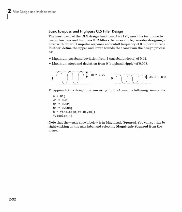
2 Filter Design and Implementation
2-3
Basic Lowpass and Highpass CLS Filter DesignThe most basic of the CLS design functions, fircls1, uses this technique to design lowpass and highpass FIR filters. As an example, consider designing a filter with order 61 impulse response and cutoff frequency of 0.3 (normalized). Further, define the upper and lower bounds that constrain the design process as:
• Maximum passband deviation from 1 (passband ripple) of 0.02.
• Maximum stopband deviation from 0 (stopband ripple) of 0.008.
To approach this design problem using fircls1, use the following commands:
n = 61;wo = 0.3;dp = 0.02;ds = 0.008;h = fircls1(n,wo,dp,ds);fvtool(h,1)
Note that the y-axis shown below is in Magnitude Squared. You can set this by right-clicking on the axis label and selecting Magnitude Squared from the menu.
0 ds = 0.0081dp = 0.02
2
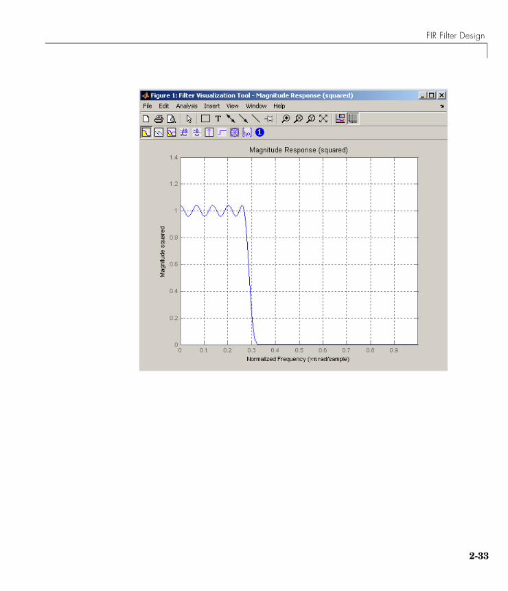
FIR Filter Design
2-33
2 Filter Design and Implementation
2-3
Multiband CLS Filter Designfircls uses the same technique to design FIR filters with a desired piecewise constant magnitude response. In this case, you can specify a vector of band edges and a corresponding vector of band amplitudes. In addition, you can specify the maximum amount of ripple for each band.
For example, assume the specifications for a filter call for:
• From 0 to 0.3 (normalized): amplitude 0, upper bound 0.005, lower bound -0.005
• From 0.3 to 0.5: amplitude 0.5, upper bound 0.51, lower bound 0.49
• From 0.5 to 0.7: amplitude 0, upper bound 0.03, lower bound -0.03
• From 0.7 to 0.9: amplitude 1, upper bound 1.02, lower bound 0.98
• From 0.9 to 1: amplitude 0, upper bound 0.05, lower bound -0.05
Design a CLS filter with impulse response order 129 that meets these specifications:
n = 129;f = [0 0.3 0.5 0.7 0.9 1];a = [0 0.5 0 1 0];up = [0.005 0.51 0.03 1.02 0.05];lo = [-0.005 0.49 -0.03 0.98 -0.05];h = fircls(n,f,a,up,lo);fvtool(h,1)
Note that the y-axis shown below is in Magnitude Squared. You can set this by right-clicking on the axis label and selecting Magnitude Squared from the menu.
4
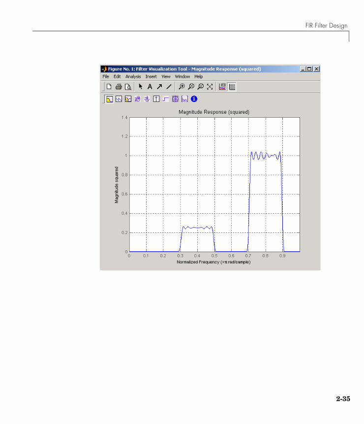
FIR Filter Design
2-35

2 Filter Design and Implementation
2-3
Weighted CLS Filter DesignWeighted CLS filter design lets you design lowpass or highpass FIR filters with relative weighting of the error minimization in each band. The fircls1 function enables you to specify the passband and stopband edges for the least squares weighting function, as well as a constant k that specifies the ratio of the stopband to passband weighting.
For example, consider specifications that call for an FIR filter with impulse response order of 55 and cutoff frequency of 0.3 (normalized). Also assume maximum allowable passband ripple of 0.02 and maximum allowable stopband ripple of 0.004. In addition, add weighting requirements:
• Passband edge for the weight function of 0.28 (normalized)
• Stopband edge for the weight function of 0.32
• Weight error minimization 10 times as much in the stopband as in the passband
To approach this using fircls1, type
n = 55;wo = 0.3;dp = 0.02;ds = 0.004;wp = 0.28;ws = 0.32;k = 10;h = fircls1(n,wo,dp,ds,wp,ws,k);fvtool(h,1)
Note that the y-axis shown below is in Magnitude Squared. You can set this by right-clicking on the axis label and selecting Magnitude Squared from the menu.
6
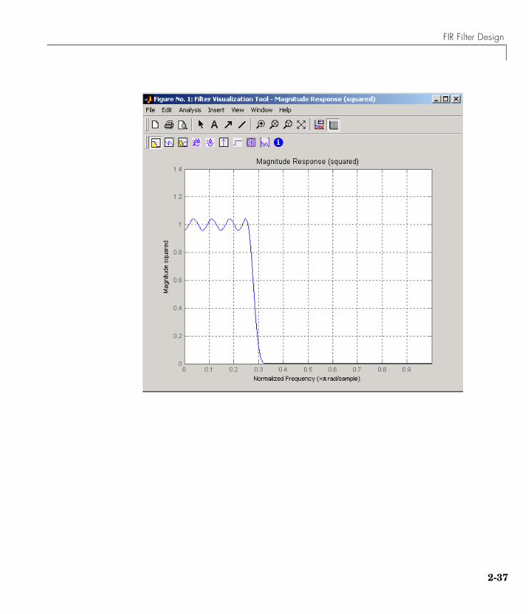
FIR Filter Design
2-37
2 Filter Design and Implementation
2-3
Arbitrary-Response Filter DesignThe cfirpm filter design function provides a tool for designing FIR filters with arbitrary complex responses. It differs from the other filter design functions in how the frequency response of the filter is specified: it accepts the name of a function which returns the filter response calculated over a grid of frequencies. This capability makes cfirpm a highly versatile and powerful technique for filter design.
This design technique may be used to produce nonlinear-phase FIR filters, asymmetric frequency-response filters (with complex coefficients), or more symmetric filters with custom frequency responses.
The design algorithm optimizes the Chebyshev (or minimax) error using an extended Remez-exchange algorithm for an initial estimate. If this exchange method fails to obtain the optimal filter, the algorithm switches to an ascent-descent algorithm that takes over to finish the convergence to the optimal solution.
Multiband Filter DesignConsider a multiband filter with the following special frequency-domain characteristics.
A linear-phase multiband filter may be designed using the predefined frequency-response function multiband, as follows:
b = cfirpm(38, [-1 -0.5 -0.4 0.3 0.4 0.8], ... 'multiband', [5 1 2 2 2 1], [1 10 5]);
Band Amplitude Optimization Weighting
[-1 -0.5] [5 1] 1
[-0.4 +0.3] [2 2] 10
[+0.4 +0.8] [2 1] 5
8
FIR Filter Design
For the specific case of a multiband filter, we can use a shorthand filter design notation similar to the syntax for firpm:
b = cfirpm(38,[-1 -0.5 -0.4 0.3 0.4 0.8], ... [5 1 2 2 2 1], [1 10 5]);
As with firpm, a vector of band edges is passed to cfirpm. This vector defines the frequency bands over which optimization is performed; note that there are two transition bands, from -0.5 to -0.4 and from 0.3 to 0.4.
In either case, the frequency response is obtained and plotted using linear scale in FVTool:
fvtool(b,1)
Note that the range of data shown below is (-Fs/2,Fs/2). You can set this range by changing the x-axis units to Frequency (Fs = 1 Hz).
2-39
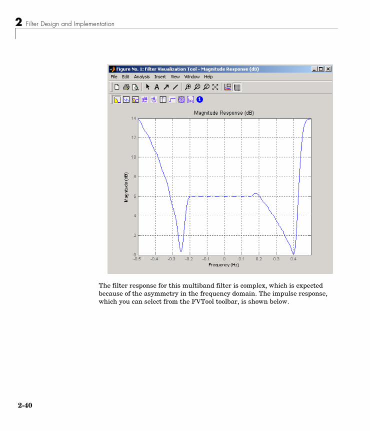
2 Filter Design and Implementation
2-4
The filter response for this multiband filter is complex, which is expected because of the asymmetry in the frequency domain. The impulse response, which you can select from the FVTool toolbar, is shown below.
0
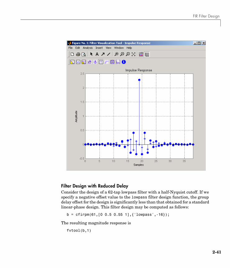
FIR Filter Design
Filter Design with Reduced DelayConsider the design of a 62-tap lowpass filter with a half-Nyquist cutoff. If we specify a negative offset value to the lowpass filter design function, the group delay offset for the design is significantly less than that obtained for a standard linear-phase design. This filter design may be computed as follows:
b = cfirpm(61,[0 0.5 0.55 1],'lowpass',-16);
The resulting magnitude response is
fvtool(b,1)
2-41
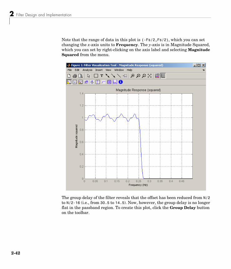
2 Filter Design and Implementation
2-4
Note that the range of data in this plot is (-Fs/2,Fs/2), which you can set changing the x-axis units to Frequency. The y-axis is in Magnitude Squared, which you can set by right-clicking on the axis label and selecting Magnitude Squared from the menu.
The group delay of the filter reveals that the offset has been reduced from N/2 to N/2-16 (i.e., from 30.5 to 14.5). Now, however, the group delay is no longer flat in the passband region. To create this plot, click the Group Delay button on the toolbar.
2
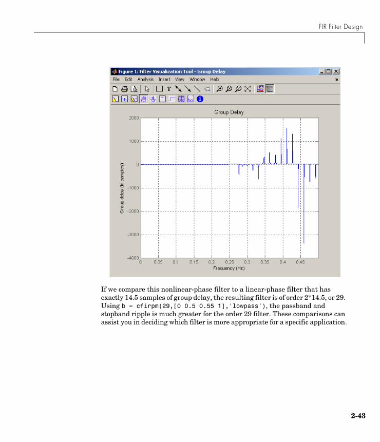
FIR Filter Design
If we compare this nonlinear-phase filter to a linear-phase filter that has exactly 14.5 samples of group delay, the resulting filter is of order 2*14.5, or 29. Using b = cfirpm(29,[0 0.5 0.55 1],'lowpass'), the passband and stopband ripple is much greater for the order 29 filter. These comparisons can assist you in deciding which filter is more appropriate for a specific application.
2-43
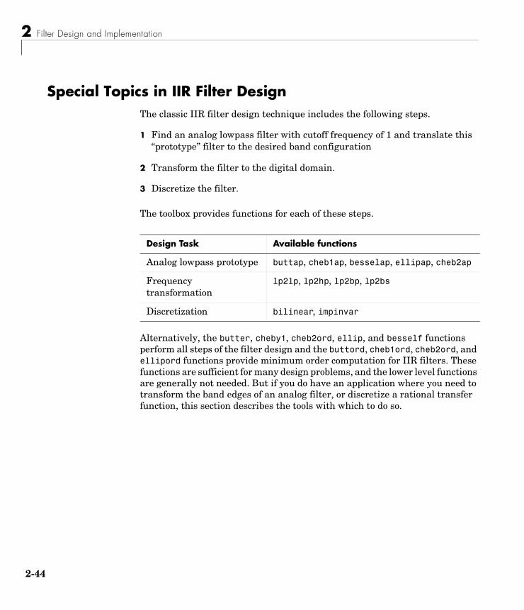
2 Filter Design and Implementation
2-4
Special Topics in IIR Filter DesignThe classic IIR filter design technique includes the following steps.
1 Find an analog lowpass filter with cutoff frequency of 1 and translate this “prototype” filter to the desired band configuration
2 Transform the filter to the digital domain.
3 Discretize the filter.
The toolbox provides functions for each of these steps.
Alternatively, the butter, cheby1, cheb2ord, ellip, and besself functions perform all steps of the filter design and the buttord, cheb1ord, cheb2ord, and ellipord functions provide minimum order computation for IIR filters. These functions are sufficient for many design problems, and the lower level functions are generally not needed. But if you do have an application where you need to transform the band edges of an analog filter, or discretize a rational transfer function, this section describes the tools with which to do so.
Design Task Available functions
Analog lowpass prototype buttap, cheb1ap, besselap, ellipap, cheb2ap
Frequency transformation
lp2lp, lp2hp, lp2bp, lp2bs
Discretization bilinear, impinvar
4
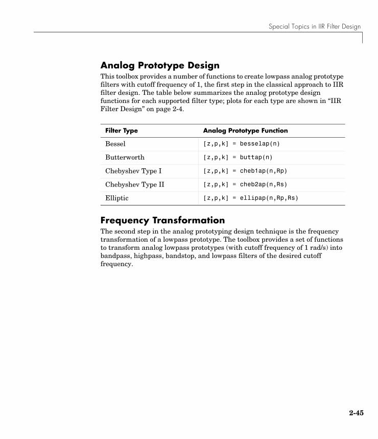
Special Topics in IIR Filter Design
Analog Prototype DesignThis toolbox provides a number of functions to create lowpass analog prototype filters with cutoff frequency of 1, the first step in the classical approach to IIR filter design. The table below summarizes the analog prototype design functions for each supported filter type; plots for each type are shown in “IIR Filter Design” on page 2-4.
Frequency TransformationThe second step in the analog prototyping design technique is the frequency transformation of a lowpass prototype. The toolbox provides a set of functions to transform analog lowpass prototypes (with cutoff frequency of 1 rad/s) into bandpass, highpass, bandstop, and lowpass filters of the desired cutoff frequency.
Filter Type Analog Prototype Function
Bessel [z,p,k] = besselap(n)
Butterworth [z,p,k] = buttap(n)
Chebyshev Type I [z,p,k] = cheb1ap(n,Rp)
Chebyshev Type II [z,p,k] = cheb2ap(n,Rs)
Elliptic [z,p,k] = ellipap(n,Rp,Rs)
2-45
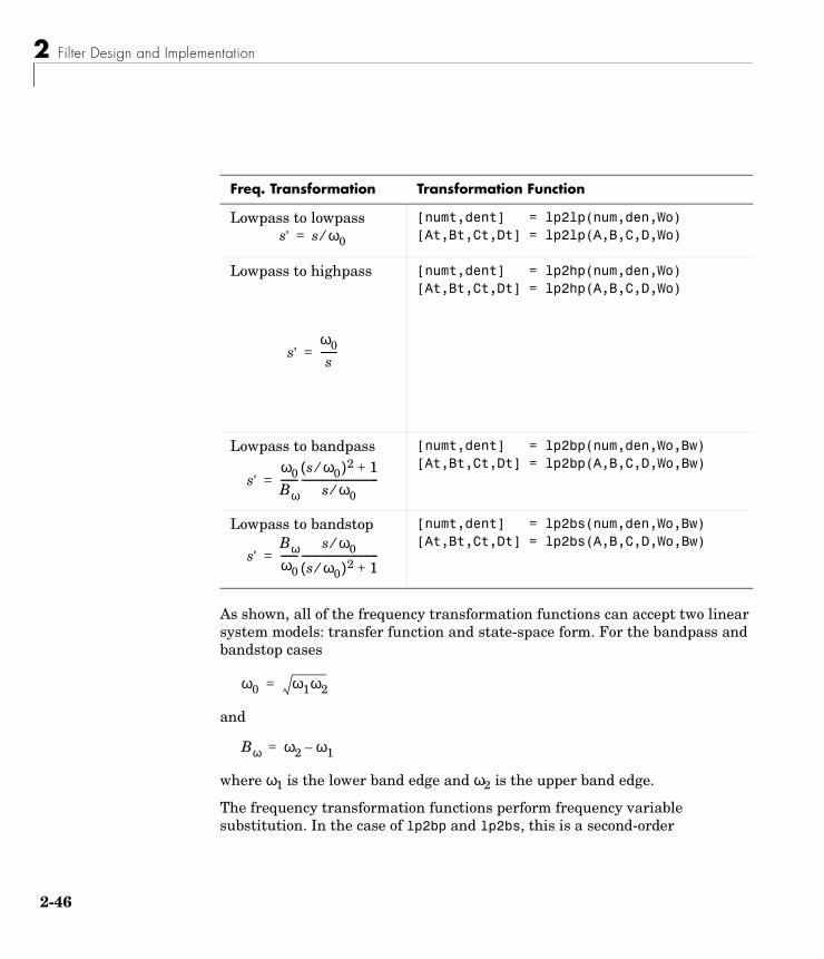
2 Filter Design and Implementation
2-4
As shown, all of the frequency transformation functions can accept two linear system models: transfer function and state-space form. For the bandpass and bandstop cases
and
where ω1 is the lower band edge and ω2 is the upper band edge.
The frequency transformation functions perform frequency variable substitution. In the case of lp2bp and lp2bs, this is a second-order
Freq. Transformation Transformation Function
Lowpass to lowpass [numt,dent] = lp2lp(num,den,Wo)[At,Bt,Ct,Dt] = lp2lp(A,B,C,D,Wo)
Lowpass to highpass [numt,dent] = lp2hp(num,den,Wo)[At,Bt,Ct,Dt] = lp2hp(A,B,C,D,Wo)
Lowpass to bandpass [numt,dent] = lp2bp(num,den,Wo,Bw)[At,Bt,Ct,Dt] = lp2bp(A,B,C,D,Wo,Bw)
Lowpass to bandstop [numt,dent] = lp2bs(num,den,Wo,Bw)[At,Bt,Ct,Dt] = lp2bs(A,B,C,D,Wo,Bw)
s' s ω0⁄=
s'ω0s
-------=
s'ω0Bω-------
s ω0⁄( )2 1+
s ω0⁄-------------------------------=
s'Bωω0-------
s ω0⁄
s ω0⁄( )2 1+-------------------------------=
ω0 ω1ω2=
Bω ω2 ω1–=
6
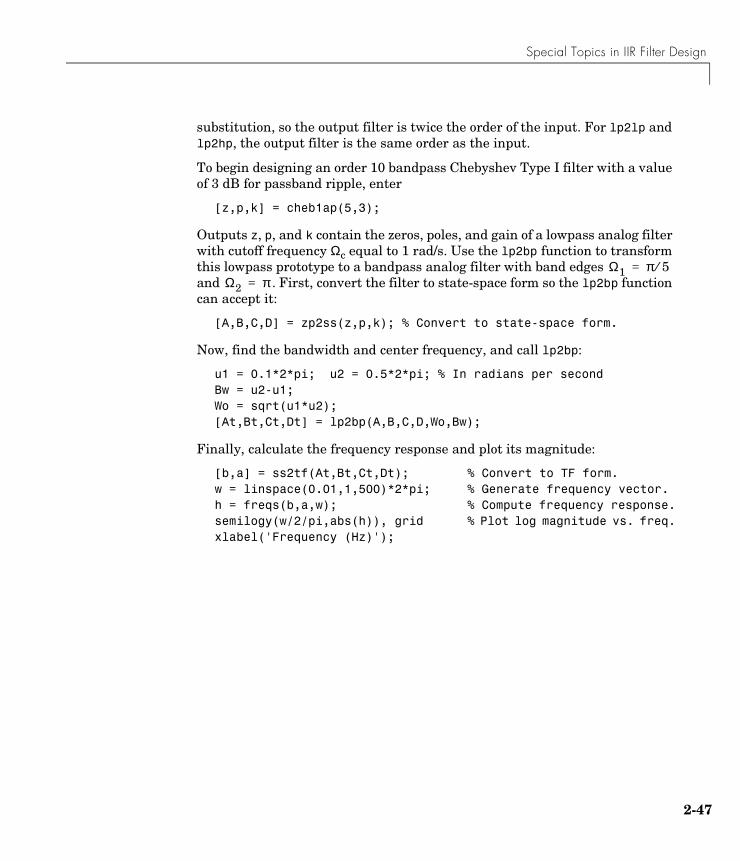
Special Topics in IIR Filter Design
substitution, so the output filter is twice the order of the input. For lp2lp and lp2hp, the output filter is the same order as the input.
To begin designing an order 10 bandpass Chebyshev Type I filter with a value of 3 dB for passband ripple, enter
[z,p,k] = cheb1ap(5,3);
Outputs z, p, and k contain the zeros, poles, and gain of a lowpass analog filter with cutoff frequency Ωc equal to 1 rad/s. Use the lp2bp function to transform this lowpass prototype to a bandpass analog filter with band edges and . First, convert the filter to state-space form so the lp2bp function can accept it:
[A,B,C,D] = zp2ss(z,p,k); % Convert to state-space form.
Now, find the bandwidth and center frequency, and call lp2bp:
u1 = 0.1*2*pi; u2 = 0.5*2*pi; % In radians per secondBw = u2-u1;Wo = sqrt(u1*u2);[At,Bt,Ct,Dt] = lp2bp(A,B,C,D,Wo,Bw);
Finally, calculate the frequency response and plot its magnitude:
[b,a] = ss2tf(At,Bt,Ct,Dt); % Convert to TF form.w = linspace(0.01,1,500)*2*pi; % Generate frequency vector.h = freqs(b,a,w); % Compute frequency response.semilogy(w/2/pi,abs(h)), grid % Plot log magnitude vs. freq.xlabel('Frequency (Hz)');
Ω1 π 5⁄=Ω2 π=
2-47
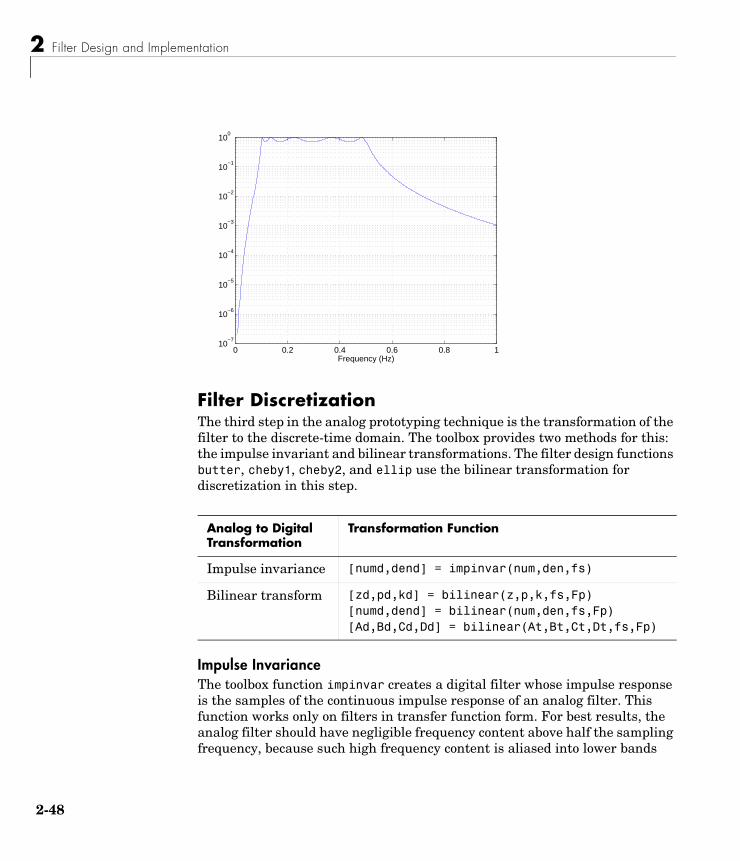
2 Filter Design and Implementation
2-4
Filter DiscretizationThe third step in the analog prototyping technique is the transformation of the filter to the discrete-time domain. The toolbox provides two methods for this: the impulse invariant and bilinear transformations. The filter design functions butter, cheby1, cheby2, and ellip use the bilinear transformation for discretization in this step.
Impulse InvarianceThe toolbox function impinvar creates a digital filter whose impulse response is the samples of the continuous impulse response of an analog filter. This function works only on filters in transfer function form. For best results, the analog filter should have negligible frequency content above half the sampling frequency, because such high frequency content is aliased into lower bands
Analog to Digital Transformation
Transformation Function
Impulse invariance [numd,dend] = impinvar(num,den,fs)
Bilinear transform [zd,pd,kd] = bilinear(z,p,k,fs,Fp)[numd,dend] = bilinear(num,den,fs,Fp)[Ad,Bd,Cd,Dd] = bilinear(At,Bt,Ct,Dt,fs,Fp)
0 0.2 0.4 0.6 0.8 110
−7
10−6
10−5
10−4
10−3
10−2
10−1
100
Frequency (Hz)
8
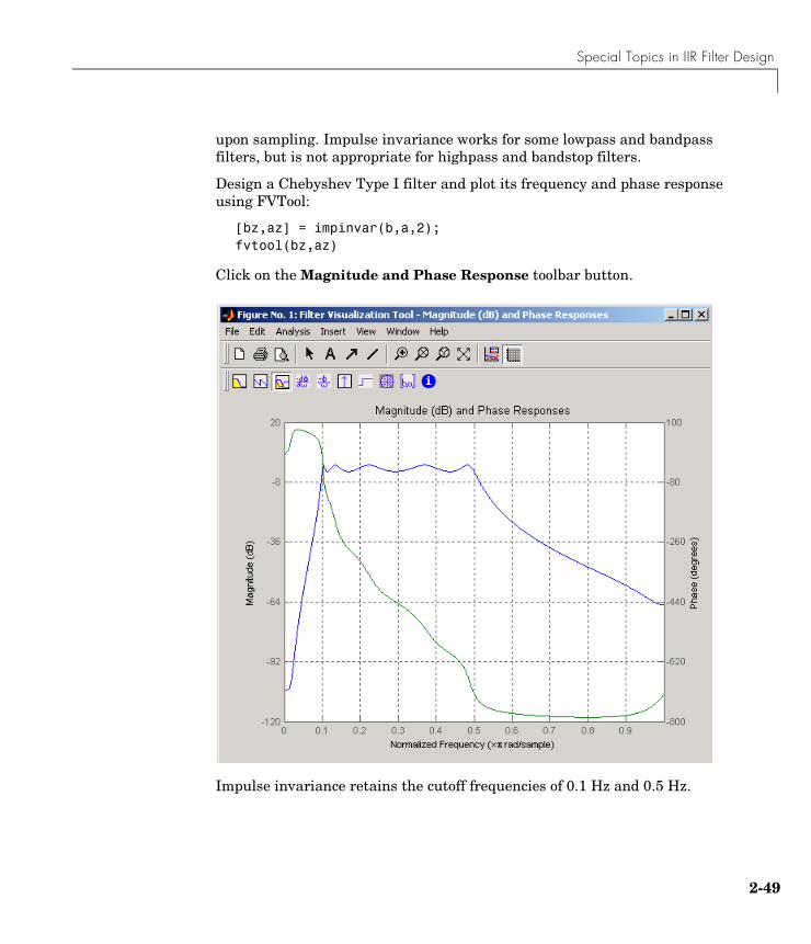
Special Topics in IIR Filter Design
upon sampling. Impulse invariance works for some lowpass and bandpass filters, but is not appropriate for highpass and bandstop filters.
Design a Chebyshev Type I filter and plot its frequency and phase response using FVTool:
[bz,az] = impinvar(b,a,2);fvtool(bz,az)
Click on the Magnitude and Phase Response toolbar button.
Impulse invariance retains the cutoff frequencies of 0.1 Hz and 0.5 Hz.
2-49
2 Filter Design and Implementation
2-5
Bilinear TransformationThe bilinear transformation is a nonlinear mapping of the continuous domain to the discrete domain; it maps the s-plane into the z-plane by
Bilinear transformation maps the -axis of the continuous domain to the unit circle of the discrete domain according to
The toolbox function bilinear implements this operation, where the frequency warping constant k is equal to twice the sampling frequency (2*fs) by default, and equal to if you give bilinear a trailing argument that represents a “match” frequency Fp. If a match frequency Fp (in hertz) is present, bilinear maps the frequency (in rad/s) to the same frequency in the discrete domain, normalized to the sampling rate:
(in rad/sample).
The bilinear function can perform this transformation on three different linear system representations: zero-pole-gain, transfer function, and state-space form. Try calling bilinear with the state-space matrices that describe the Chebyshev Type I filter from the previous section, using a sampling frequency of 2 Hz, and retaining the lower band edge of 0.1 Hz:
[Ad,Bd,Cd,Dd] = bilinear(At,Bt,Ct,Dt,2,0.1);
The frequency response of the resulting digital filter is
[bz,az] = ss2tf(Ad,Bd,Cd,Dd); % convert to TFfvtool(bz,az)
Click on the Magnitude and Phase Response toolbar button.
H z( ) H s( )s kz 1–
z 1+------------=
=
jΩ
ω 2tan 1– Ωk---- =
2πfp πfp fs⁄( )tan⁄
Ω 2πfp=
ω 2πfp fs⁄=
0
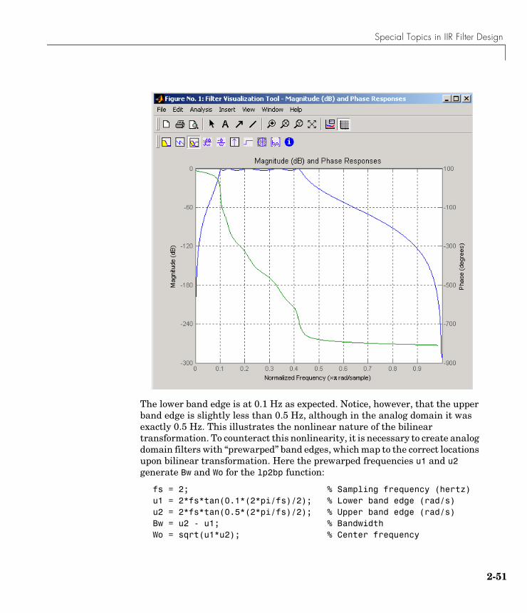
Special Topics in IIR Filter Design
The lower band edge is at 0.1 Hz as expected. Notice, however, that the upper band edge is slightly less than 0.5 Hz, although in the analog domain it was exactly 0.5 Hz. This illustrates the nonlinear nature of the bilinear transformation. To counteract this nonlinearity, it is necessary to create analog domain filters with “prewarped” band edges, which map to the correct locations upon bilinear transformation. Here the prewarped frequencies u1 and u2 generate Bw and Wo for the lp2bp function:
fs = 2; % Sampling frequency (hertz)u1 = 2*fs*tan(0.1*(2*pi/fs)/2); % Lower band edge (rad/s)u2 = 2*fs*tan(0.5*(2*pi/fs)/2); % Upper band edge (rad/s)Bw = u2 - u1; % BandwidthWo = sqrt(u1*u2); % Center frequency
2-51

2 Filter Design and Implementation
2-5
[At,Bt,Ct,Dt] = lp2bp(A,B,C,D,Wo,Bw);
A digital bandpass filter with correct band edges 0.1 and 0.5 times the Nyquist frequency is
[Ad,Bd,Cd,Dd] = bilinear(At,Bt,Ct,Dt,fs);
The example bandpass filters from the last two sections could also be created in one statement using the complete IIR design function cheby1. For instance, an analog version of the example Chebyshev filter is
[b,a] = cheby1(5,3,[0.1 0.5]*2*pi,'s');
Note that the band edges are in rad/s for analog filters, whereas for the digital case, frequency is normalized:
[bz,az] = cheby1(5,3,[0.1 0.5]);
All of the complete design functions call bilinear internally. They prewarp the band edges as needed to obtain the correct digital filter.
2
Filter Implementation
Filter ImplementationAfter the filter design process has generated the filter coefficient vectors, b and a, two functions are available in the Signal Processing Toolbox for implementing your filter:
• dfilt—lets you specify the filter structure and creates a digital filter object.
• filter—for b and a coefficient input, implements a direct-form II transposed structure and filters the data. For dfilt input, filter uses the structure specified with dfilt and filters the data.
Note Using filter on b and a coefficients normalizes the filter by forcing the a0 coefficient to be equal to 1. Using filter on a dfilt object does not normalize the filter.
Choosing the best filter structure depends on the task the filter will perform. Some structures are more suited to or may be more computationally efficient for particular tasks. For example, often it is not possible to build recursive (IIR) filters to run at very high speeds and instead, you would use a nonrecursive (FIR) filter. FIR filters are always stable and have well-behaved roundoff noise characteristics. Direct-form IIR filters are usually realized in second-order-sections because they are sensitive to roundoff noise.
Using dfiltImplementing your digital filter using dfilt lets you specify the filter structure and creates a single filter object from the filter coefficient vectors. dfilt objects have many predefined methods which can provide information about the filter that is not easily obtained directly from the filter coefficients alone. For a complete list of these methods and for more information, see dfilt.
2-53

2 Filter Design and Implementation
2-5
After you have created a dfilt object, you can use filter to apply your implemented filter to data. The complete process of designing, implementing, and applying a filter using a dfilt object is described below:
1 Generate the filter coefficients using any IIR or FIR filter design function.
2 Create the filter object from the filter coefficients and the specified filter structure using dfilt.
3 Apply the dfilt filter object to the data, x using filter.
For example, to design, implement as a direct-form II transposed structure, and apply a Butterworth filter to the data in x:
[b,a] = butter(5,0.4);Hd = dfilt.df2t(b,a); %Implement direct-form II transposedfilter(Hd,x)
Another way to implement a direct-form II structure is with filter:
[b,a] = butter(5,0.4);filter(b,a,x)
Note filter implements only a direct-form II structure and does not create a filter object.
4

Selected Bibliography
Selected Bibliography[1] Karam, L.J., and J.H. McClellan. “Complex Chebyshev Approximation for FIR Filter Design.” IEEE Trans. on Circuits and Systems II. March 1995.
[2] Selesnick, I.W., and C.S. Burrus. “Generalized Digital Butterworth Filter Design.” Proceedings of the IEEE Int. Conf. Acoust., Speech, Signal Processing. Vol. 3 (May 1996).
[3] Selesnick, I.W., M. Lang, and C.S. Burrus. “Constrained Least Square Design of FIR Filters without Specified Transition Bands.” Proceedings of the IEEE Int. Conf. Acoust., Speech, Signal Processing. Vol. 2 (May 1995). Pgs. 1260-1263.
2-55

2 Filter Design and Implementation
2-5
6
3
Statistical Signal ProcessingThe following chapter discusses statistical signal processing tools and applications, including correlations, covariance, and spectral estimation.
Correlation and Covariance (p. 3-2) Correlation and covariance background information and toolbox functions
Spectral Analysis (p. 3-5) Spectral estimation techniques and toolbox functions
Selected Bibliography (p. 3-45) Sources of additional information
3 Statistical Signal Processing
3-2
Correlation and CovarianceThe functions xcorr and xcov estimate the cross-correlation and cross-covariance sequences of random processes. They also handle autocorrelation and autocovariance as special cases.
The true cross-correlation sequence is a statistical quantity defined as
where xn and yn are stationary random processes, , and E⋅ is the expected value operator. The covariance sequence is the mean-removed cross-correlation sequence
or, in terms of the cross-correlation,
In practice, you must estimate these sequences, because it is possible to access only a finite segment of the infinite-length random process. A common estimate based on N samples of xn and yn is the deterministic cross-correlation sequence (also called the time-ambiguity function)
where we assume for this discussion that xn and yn are indexed from 0 to N-1,
and from -(N-1) to N-1. The xcorr function evaluates this sum with an efficient FFT-based algorithm, given inputs xn and yn stored in length N vectors x and y. Its operation is equivalent to convolution with one of the two subsequences reversed in time.
Rxy m( ) Exn m+ y*n Exny*n m– ==
∞– n ∞< <
Cxy m( ) E xn m+ µx–( ) yn µy–( )*=
Cxy m( ) Rxy m( ) µxµ*y–=
Rˆ
xy m( )xn m+ yn
*
n 0=
N m– 1–
∑ m 0≥
Rˆ
yx*
m–( ) m 0<
=
Rˆ
xy m( )
Correlation and Covariance
For example:
x = [1 1 1 1 1]';y = x;xyc = xcorr(x,y)
xyc =
1.0000 2.0000 3.0000 4.0000 5.0000 4.0000 3.0000 2.0000 1.0000
Notice that the resulting sequence length is one less than twice the length of the input sequence. Thus, the Nth element is the correlation at lag 0. Also notice the triangular pulse of the output that results when convolving two square pulses.
The xcov function estimates autocovariance and cross-covariance sequences. This function has the same options and evaluates the same sum as xcorr, but first removes the means of x and y.
Bias and NormalizationAn estimate of a quantity is biased if its expected value is not equal to the quantity it estimates. The expected value of the output of xcorr is
xcorr provides the unbiased estimate, dividing by N-|m|, when you specify an 'unbiased' flag after the input sequences.
xcorr(x,y,'unbiased')
ERˆ
xy m( ) Exn m+ y*n
n 0=
N m– 1–
∑ N m–( )Rxy m( )= =
3-3
3 Statistical Signal Processing
3-4
Although this estimate is unbiased, the end points (near -(N-1) and N-1) suffer from large variance because xcorr computes them using only a few data points. A possible trade-off is to simply divide by N using the 'biased' flag:
xcorr(x,y,'biased')
With this scheme, only the sample of the correlation at zero lag (the Nth output element) is unbiased. This estimate is often more desirable than the unbiased one because it avoids random large variations at the end points of the correlation sequence.
xcorr provides one other normalization scheme. The syntax
xcorr(x,y,'coeff')
divides the output by norm(x)*norm(y) so that, for autocorrelations, the sample at zero lag is 1.
Multiple ChannelsFor a multichannel signal, xcorr and xcov estimate the autocorrelation and cross-correlation and covariance sequences for all of the channels at once. If S is an M-by-N signal matrix representing N channels in its columns, xcorr(S) returns a (2M-1)-by-N2 matrix with the autocorrelations and cross-correlations of the channels of S in its N2 columns. If S is a three-channel signal
S = [s1 s2 s3]
then the result of xcorr(S) is organized as
R = [Rs1s1 Rs1s2 Rs1s3 Rs2s1 Rs2s2 Rs2s3 Rs3s1 Rs3s2 Rs3s3]
Two related functions, cov and corrcoef, are available in the standard MATLAB environment. They estimate covariance and normalized covariance respectively between the different channels at lag 0 and arrange them in a square matrix.
Spectral Analysis
Spectral AnalysisThe goal of spectral estimation is to describe the distribution (over frequency) of the power contained in a signal, based on a finite set of data. Estimation of power spectra is useful in a variety of applications, including the detection of signals buried in wide-band noise.
The power spectrum of a stationary random process xn is mathematically related to the correlation sequence by the discrete-time Fourier transform. In terms of normalized frequency, this is given by
This can be written as a function of physical frequency f (e.g., in hertz) by using the relation ω = 2πf/fs, where fs is the sampling frequency.
The correlation sequence can be derived from the power spectrum by use of the inverse discrete-time Fourier transform:
The average power of the sequence xn over the entire Nyquist interval is represented by
Sxx ω( ) Rxx m( )e jωm–
m ∞–=
∞
∑=
Sxx f( ) Rxx m( )e 2πjfm– fs⁄
m ∞–=
∞
∑=
Rxx m( )Sxx ω( )ejωm
2π------------------------------ ωd
π–
π
∫Sxx f( )e2πjfm fs⁄
fs--------------------------------------- fd
fs 2⁄–
fs 2⁄
∫= =
Rxx 0( )Sxx ω( )
2π----------------- ωd
π–
π
∫Sxx f( )
fs--------------- fd
fs 2⁄–
fs 2⁄
∫= =
3-5
3 Statistical Signal Processing
3-6
The quantities
from the above expression are defined as the power spectral density (PSD) of the stationary random signal xn.
The average power of a signal over a particular frequency band , , can be found by integrating the PSD over that band:
You can see from the above expression that Pxx(ω) represents the power content of a signal in an infinitesimal frequency band, which is why it is called the power spectral density.
The units of the PSD are power (e.g., watts) per unit of frequency. In the case of Pxx(ω), this is watts/radian/sample or simply watts/radian. In the case of Pxx(f), the units are watts/hertz. Integration of the PSD with respect to frequency yields units of watts, as expected for the average power .
For real signals, the PSD is symmetric about DC, and thus Pxx(ω) for is sufficient to completely characterize the PSD. However, to obtain the average power over the entire Nyquist interval, it is necessary to introduce the concept of the one-sided PSD.
The one-sided PSD is given by
The average power of a signal over the frequency band , , can be computed using the one-sided PSD as
Pxx ω( )Sxx ω( )
2π-----------------= Pxx f( )
Sxx f( )
fs---------------=and
ω1 ω2[ , ]0 ω1 ω2 π≤<≤
P ω1 ω2,[ ] Pxx ω( ) ωd
ω1
ω2
∫ Pxx ω( ) ωd
ω– 2
ω– 1
∫+=
P ω1 ω2,[ ]
0 ω π<≤
Ponesided ω( )0 -π ω≤ 0<,2Pxx ω( ) 0 ω≤ π<,
=
ω1 ω2[ , ] 0 ω1 ω2 π≤<≤
P ω1 ω2,[ ] Ponesided ω( ) ωd
ω1
ω2
∫=
Spectral Analysis
Spectral Estimation MethodThe various methods of spectrum estimation available in the Signal Processing Toolbox are categorized as follows:
• Nonparametric methods
• Parametric methods
• Subspace methods
Nonparametric methods are those in which the PDS is estimated directly from the signal itself. The simplest such method is the periodogram. An improved version of the periodogram is Welch’s method [8]. A more modern nonparametric technique is the multitaper method (MTM).
Parametric methods are those in which the PSD is estimated from a signal that is is assumed to be output of a linear system driven by white noise. Examples are the Yule-Walker autoregressive (AR) method and the Burg method. These methods estimate the PSD by first estimating the parameters (coefficients) of the linear system that hypothetically “generates” the signal. They tend to produce better results than classical nonparametric methods when the data length of the available signal is relatively short.
Subspace methods, also known as high-resolution methods or super-resolution methods, generate frequency component estimates for a signal based on an eigenanalysis or eigendecomposition of the correlation matrix. Examples are the multiple signal classification (MUSIC) method or the eigenvector (EV) method. These methods are best suited for line spectra — that is, spectra of sinusoidal signals — and are effective in the detection of sinusoids buried in noise, especially when the signal to noise ratios are low.
All three categories of methods are listed in the table below with the corresponding toolbox function and spectrum object names. See “Parametric
3-7
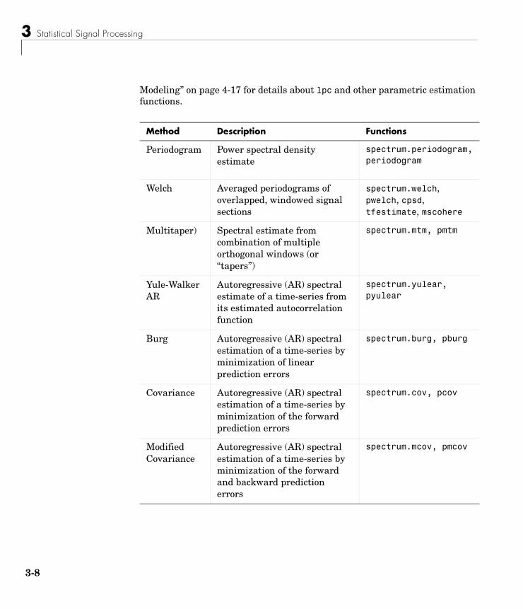
3 Statistical Signal Processing
3-8
Modeling” on page 4-17 for details about lpc and other parametric estimation functions.
Method Description Functions
Periodogram Power spectral density estimate
spectrum.periodogram, periodogram
Welch Averaged periodograms of overlapped, windowed signal sections
spectrum.welch, pwelch, cpsd, tfestimate, mscohere
Multitaper) Spectral estimate from combination of multiple orthogonal windows (or “tapers”)
spectrum.mtm, pmtm
Yule-Walker AR
Autoregressive (AR) spectral estimate of a time-series from its estimated autocorrelation function
spectrum.yulear, pyulear
Burg Autoregressive (AR) spectral estimation of a time-series by minimization of linear prediction errors
spectrum.burg, pburg
Covariance Autoregressive (AR) spectral estimation of a time-series by minimization of the forward prediction errors
spectrum.cov, pcov
Modified Covariance
Autoregressive (AR) spectral estimation of a time-series by minimization of the forward and backward prediction errors
spectrum.mcov, pmcov
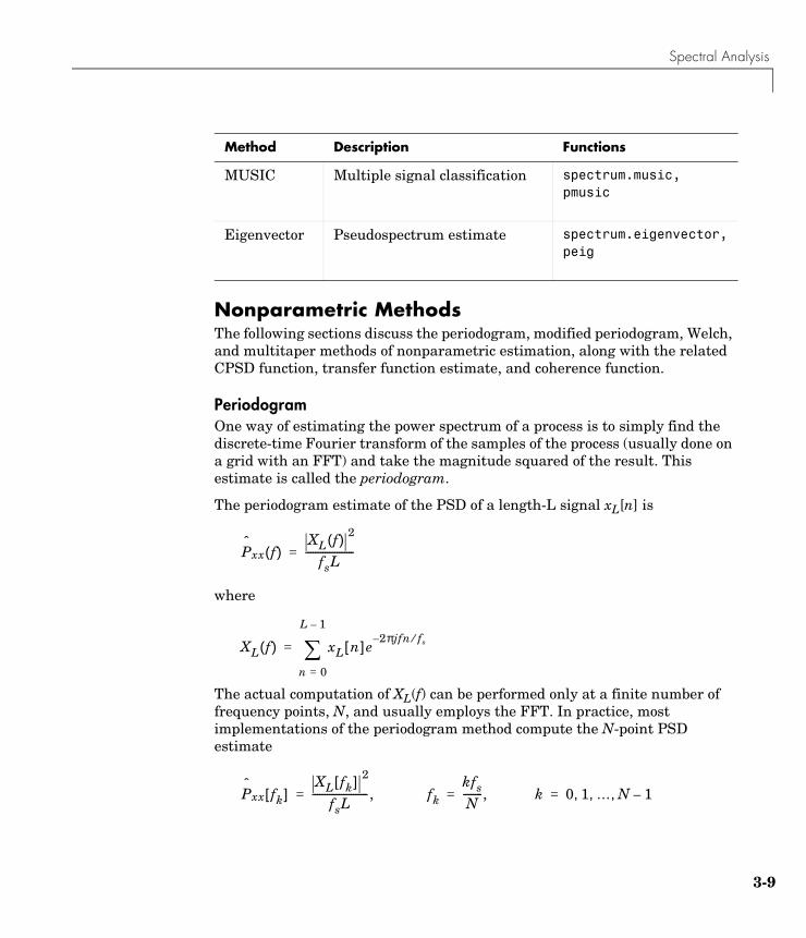
Spectral Analysis
Nonparametric MethodsThe following sections discuss the periodogram, modified periodogram, Welch, and multitaper methods of nonparametric estimation, along with the related CPSD function, transfer function estimate, and coherence function.
PeriodogramOne way of estimating the power spectrum of a process is to simply find the discrete-time Fourier transform of the samples of the process (usually done on a grid with an FFT) and take the magnitude squared of the result. This estimate is called the periodogram.
The periodogram estimate of the PSD of a length-L signal xL[n] is
where
The actual computation of XL(f) can be performed only at a finite number of frequency points, N, and usually employs the FFT. In practice, most implementations of the periodogram method compute the N-point PSD estimate
MUSIC Multiple signal classification spectrum.music, pmusic
Eigenvector Pseudospectrum estimate spectrum.eigenvector, peig
Method Description Functions
Pˆ
xx f( )XL f( ) 2
fsL--------------------=
XL f( ) xL n[ ] e2πjfn– fs⁄
n 0=
L 1–
∑=
Pˆ
xx fk[ ]XL fk[ ] 2
fsL----------------------- ,= fk
kfsN
--------,= k 0 1 … N 1–, , ,=
3-9
3 Statistical Signal Processing
3-1
where
It is wise to choose N > L so that N is the next power of two larger than L. To evaluate XL[fk], we simply pad xL[n] with zeros to length N. If L > N, we must wrap xL[n] modulo-N prior to computing XL[fk].
As an example, consider the following 1001-element signal xn, which consists of two sinusoids plus noise:
randn('state',0);fs = 1000; % Sampling frequencyt = (0:fs)/fs; % One second worth of samplesA = [1 2]; % Sinusoid amplitudes (row vector)f = [150;140]; % Sinusoid frequencies (column vector)xn = A*sin(2*pi*f*t) + 0.1*randn(size(t));
Note The three last lines illustrate a convenient and general way to express the sum of sinusoids. Together they are equivalent to
xn = sin(2*pi*150*t) + 2*sin(2*pi*140*t) + 0.1*randn(size(t));
The periodogram estimate of the PSD can be computed by creating a periodogram object
Hs = spectrum.periodogram('Hamming');
and a plot of the estimate can be displayed with the psd method:
psd(Hs,xn,'Fs',fs,'NFFT',1024,'SpectrumType','twosided')
XL fk[ ] xL n[ ] e 2πjkn– N⁄
n 0=
N 1–
∑=
0
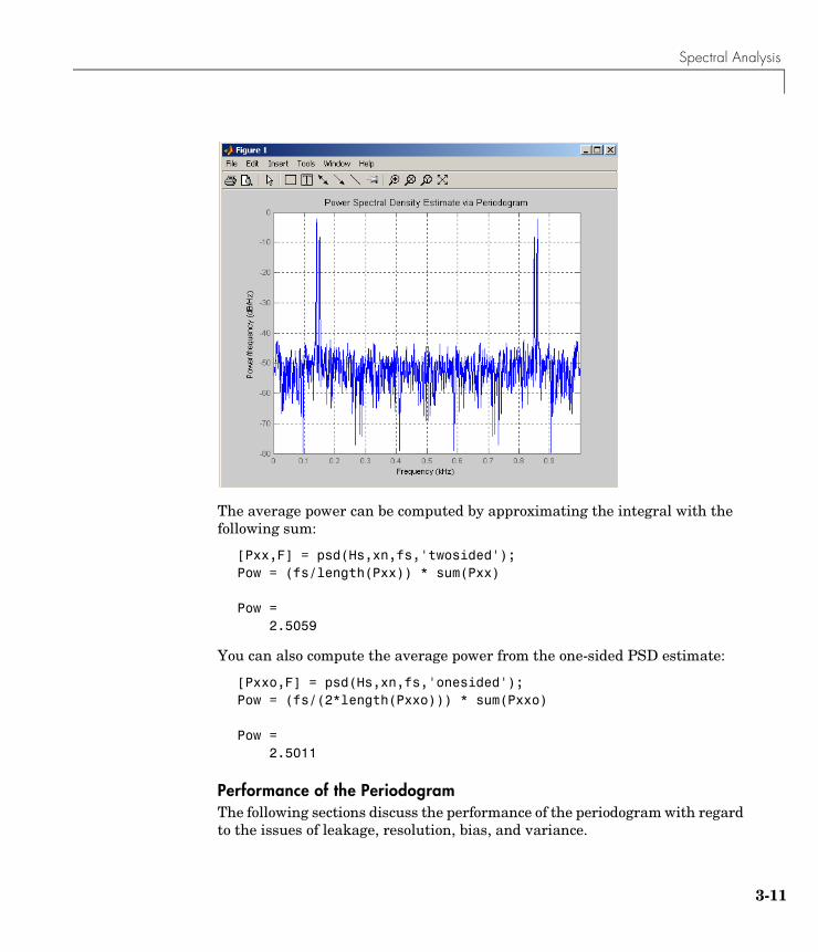
Spectral Analysis
The average power can be computed by approximating the integral with the following sum:
[Pxx,F] = psd(Hs,xn,fs,'twosided');Pow = (fs/length(Pxx)) * sum(Pxx)
Pow = 2.5059
You can also compute the average power from the one-sided PSD estimate:
[Pxxo,F] = psd(Hs,xn,fs,'onesided');Pow = (fs/(2*length(Pxxo))) * sum(Pxxo)
Pow = 2.5011
Performance of the PeriodogramThe following sections discuss the performance of the periodogram with regard to the issues of leakage, resolution, bias, and variance.
3-11
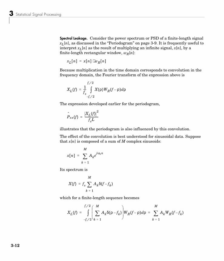
3 Statistical Signal Processing
3-1
Spectral Leakage. Consider the power spectrum or PSD of a finite-length signal xL[n], as discussed in the “Periodogram” on page 3-9. It is frequently useful to interpret xL[n] as the result of multiplying an infinite signal, x[n], by a finite-length rectangular window, wR[n]:
Because multiplication in the time domain corresponds to convolution in the frequency domain, the Fourier transform of the expression above is
The expression developed earlier for the periodogram,
illustrates that the periodogram is also influenced by this convolution.
The effect of the convolution is best understood for sinusoidal data. Suppose that x[n] is composed of a sum of M complex sinusoids:
Its spectrum is
which for a finite-length sequence becomes
xL n[ ] x n[ ] wR n[ ]⋅=
XL f( ) 1fs---- X ρ( )WR f ρ–( ) ρd
fs 2⁄–
fs 2⁄
∫=
Pˆ
xx f( )XL f( ) 2
fsL--------------------=
x n[ ] Akejωkn
k 1=
M
∑=
X f( ) fs Akδ f fk–( )
k 1=
M
∑=
XL f( ) Akδ ρ fk–( )
k 1=
M
∑
WR f ρ–( ) ρd
fs 2⁄–
fs 2⁄
∫ AkWR f fk–( )
k 1=
M
∑= =
2
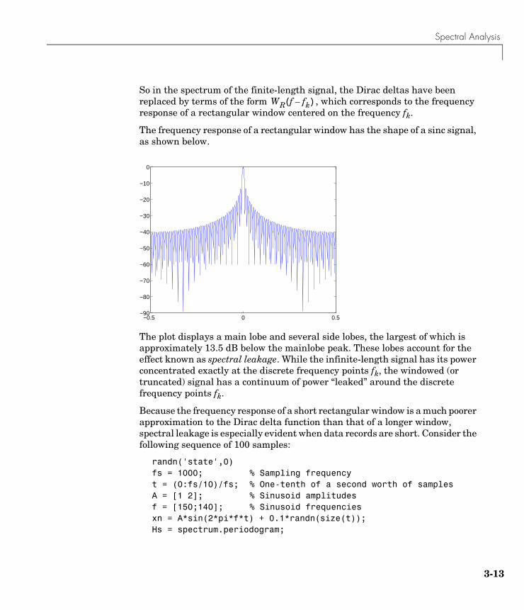
Spectral Analysis
So in the spectrum of the finite-length signal, the Dirac deltas have been replaced by terms of the form , which corresponds to the frequency response of a rectangular window centered on the frequency fk.
The frequency response of a rectangular window has the shape of a sinc signal, as shown below.
The plot displays a main lobe and several side lobes, the largest of which is approximately 13.5 dB below the mainlobe peak. These lobes account for the effect known as spectral leakage. While the infinite-length signal has its power concentrated exactly at the discrete frequency points fk, the windowed (or truncated) signal has a continuum of power “leaked” around the discrete frequency points fk.
Because the frequency response of a short rectangular window is a much poorer approximation to the Dirac delta function than that of a longer window, spectral leakage is especially evident when data records are short. Consider the following sequence of 100 samples:
randn('state',0)fs = 1000; % Sampling frequencyt = (0:fs/10)/fs; % One-tenth of a second worth of samplesA = [1 2]; % Sinusoid amplitudesf = [150;140]; % Sinusoid frequenciesxn = A*sin(2*pi*f*t) + 0.1*randn(size(t));Hs = spectrum.periodogram;
WR f fk–( )
−0.5 0 0.5−90
−80
−70
−60
−50
−40
−30
−20
−10
0
3-13
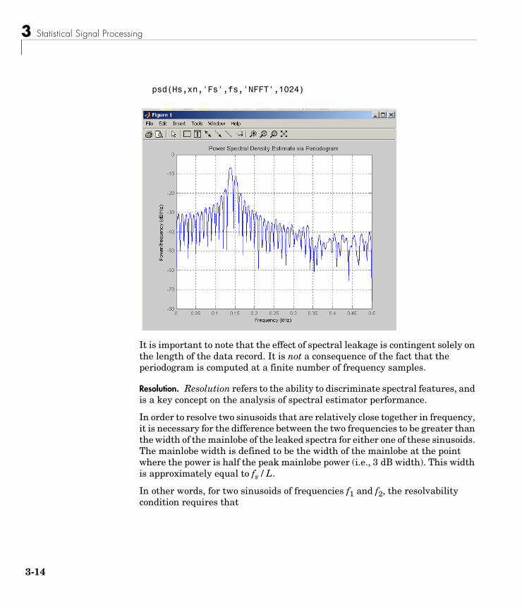
3 Statistical Signal Processing
3-1
psd(Hs,xn,'Fs',fs,'NFFT',1024)
It is important to note that the effect of spectral leakage is contingent solely on the length of the data record. It is not a consequence of the fact that the periodogram is computed at a finite number of frequency samples.
Resolution. Resolution refers to the ability to discriminate spectral features, and is a key concept on the analysis of spectral estimator performance.
In order to resolve two sinusoids that are relatively close together in frequency, it is necessary for the difference between the two frequencies to be greater than the width of the mainlobe of the leaked spectra for either one of these sinusoids. The mainlobe width is defined to be the width of the mainlobe at the point where the power is half the peak mainlobe power (i.e., 3 dB width). This width is approximately equal to fs / L.
In other words, for two sinusoids of frequencies f1 and f2, the resolvability condition requires that
4
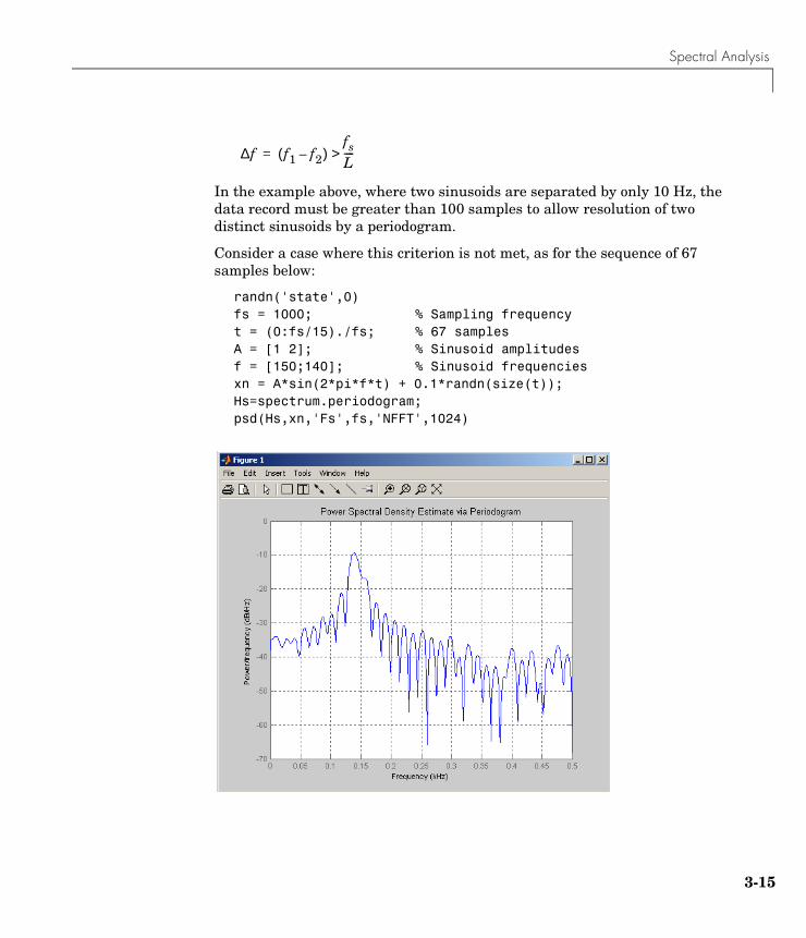
Spectral Analysis
In the example above, where two sinusoids are separated by only 10 Hz, the data record must be greater than 100 samples to allow resolution of two distinct sinusoids by a periodogram.
Consider a case where this criterion is not met, as for the sequence of 67 samples below:
randn('state',0)fs = 1000; % Sampling frequencyt = (0:fs/15)./fs; % 67 samplesA = [1 2]; % Sinusoid amplitudesf = [150;140]; % Sinusoid frequenciesxn = A*sin(2*pi*f*t) + 0.1*randn(size(t));Hs=spectrum.periodogram;psd(Hs,xn,'Fs',fs,'NFFT',1024)
∆f f1 f2–( )fsL---->=
3-15
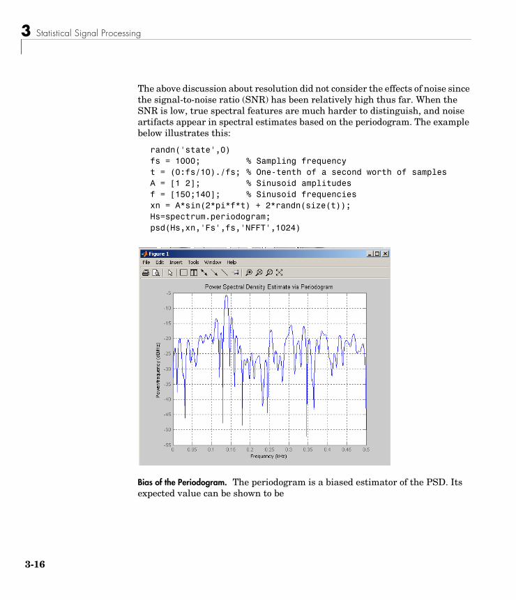
3 Statistical Signal Processing
3-1
The above discussion about resolution did not consider the effects of noise since the signal-to-noise ratio (SNR) has been relatively high thus far. When the SNR is low, true spectral features are much harder to distinguish, and noise artifacts appear in spectral estimates based on the periodogram. The example below illustrates this:
randn('state',0)fs = 1000; % Sampling frequencyt = (0:fs/10)./fs; % One-tenth of a second worth of samplesA = [1 2]; % Sinusoid amplitudesf = [150;140]; % Sinusoid frequenciesxn = A*sin(2*pi*f*t) + 2*randn(size(t));Hs=spectrum.periodogram;psd(Hs,xn,'Fs',fs,'NFFT',1024)
Bias of the Periodogram. The periodogram is a biased estimator of the PSD. Its expected value can be shown to be
6
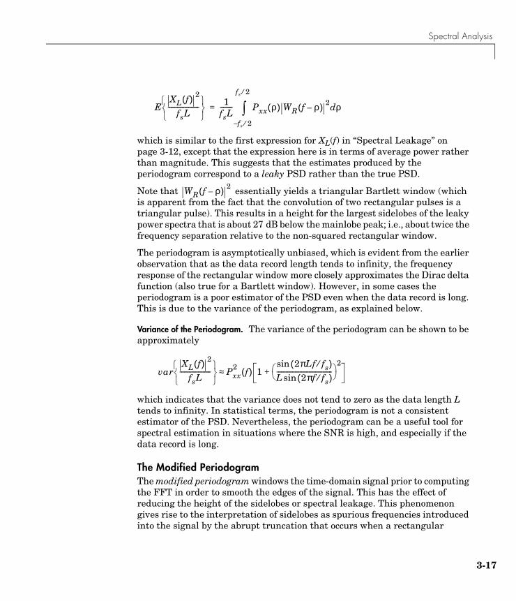
Spectral Analysis
which is similar to the first expression for XL(f) in “Spectral Leakage” on page 3-12, except that the expression here is in terms of average power rather than magnitude. This suggests that the estimates produced by the periodogram correspond to a leaky PSD rather than the true PSD.
Note that essentially yields a triangular Bartlett window (which is apparent from the fact that the convolution of two rectangular pulses is a triangular pulse). This results in a height for the largest sidelobes of the leaky power spectra that is about 27 dB below the mainlobe peak; i.e., about twice the frequency separation relative to the non-squared rectangular window.
The periodogram is asymptotically unbiased, which is evident from the earlier observation that as the data record length tends to infinity, the frequency response of the rectangular window more closely approximates the Dirac delta function (also true for a Bartlett window). However, in some cases the periodogram is a poor estimator of the PSD even when the data record is long. This is due to the variance of the periodogram, as explained below.
Variance of the Periodogram. The variance of the periodogram can be shown to be approximately
which indicates that the variance does not tend to zero as the data length L tends to infinity. In statistical terms, the periodogram is not a consistent estimator of the PSD. Nevertheless, the periodogram can be a useful tool for spectral estimation in situations where the SNR is high, and especially if the data record is long.
The Modified PeriodogramThe modified periodogram windows the time-domain signal prior to computing the FFT in order to smooth the edges of the signal. This has the effect of reducing the height of the sidelobes or spectral leakage. This phenomenon gives rise to the interpretation of sidelobes as spurious frequencies introduced into the signal by the abrupt truncation that occurs when a rectangular
EXL f( ) 2
fsL--------------------
1
fsL-------- Pxx ρ( ) WR f ρ–( ) 2 ρd
fs 2⁄–
fs 2⁄
∫=
WR f ρ–( ) 2
varXL f( ) 2
fsL--------------------
Pxx2 f( ) 1
2πLf fs⁄( )sinL 2πf fs⁄( )sin------------------------------------
2+≈
3-17
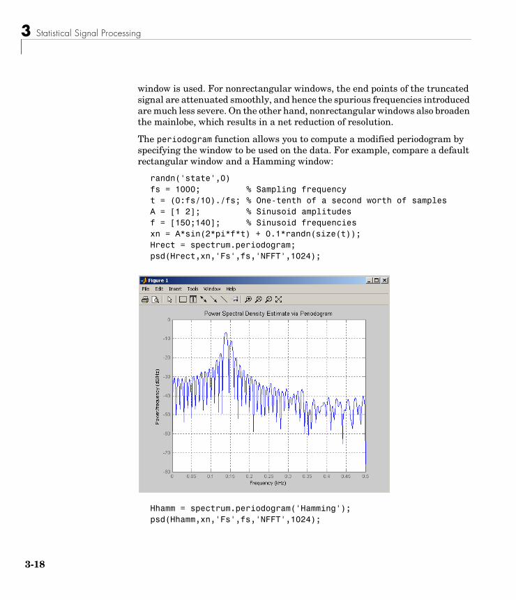
3 Statistical Signal Processing
3-1
window is used. For nonrectangular windows, the end points of the truncated signal are attenuated smoothly, and hence the spurious frequencies introduced are much less severe. On the other hand, nonrectangular windows also broaden the mainlobe, which results in a net reduction of resolution.
The periodogram function allows you to compute a modified periodogram by specifying the window to be used on the data. For example, compare a default rectangular window and a Hamming window:
randn('state',0)fs = 1000; % Sampling frequencyt = (0:fs/10)./fs; % One-tenth of a second worth of samplesA = [1 2]; % Sinusoid amplitudesf = [150;140]; % Sinusoid frequenciesxn = A*sin(2*pi*f*t) + 0.1*randn(size(t));Hrect = spectrum.periodogram;psd(Hrect,xn,'Fs',fs,'NFFT',1024);
Hhamm = spectrum.periodogram('Hamming');psd(Hhamm,xn,'Fs',fs,'NFFT',1024);
8
Spectral Analysis
You can verify that although the sidelobes are much less evident in the Hamming-windowed periodogram, the two main peaks are wider. In fact, the 3 dB width of the mainlobe corresponding to a Hamming window is approximately twice that of a rectangular window. Hence, for a fixed data length, the PSD resolution attainable with a Hamming window is approximately half that attainable with a rectangular window. The competing interests of mainlobe width and sidelobe height can be resolved to some extent by using variable windows such as the Kaiser window.
Nonrectangular windowing affects the average power of a signal because some of the time samples are attenuated when multiplied by the window. To compensate for this, the periodogram function normalizes the window to have an average power of unity. This way the choice of window does not affect the average power of the signal.
The modified periodogram estimate of the PSD is
Pˆ
xx f( )XL f( ) 2
fsLU--------------------=
3-19
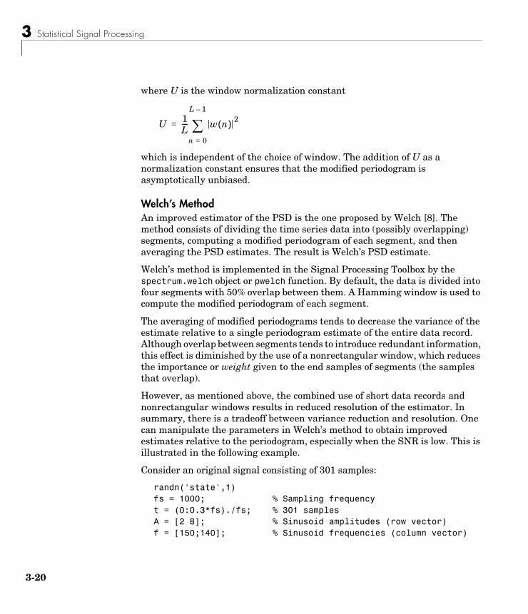
3 Statistical Signal Processing
3-2
where U is the window normalization constant
which is independent of the choice of window. The addition of U as a normalization constant ensures that the modified periodogram is asymptotically unbiased.
Welch’s MethodAn improved estimator of the PSD is the one proposed by Welch [8]. The method consists of dividing the time series data into (possibly overlapping) segments, computing a modified periodogram of each segment, and then averaging the PSD estimates. The result is Welch’s PSD estimate.
Welch’s method is implemented in the Signal Processing Toolbox by the spectrum.welch object or pwelch function. By default, the data is divided into four segments with 50% overlap between them. A Hamming window is used to compute the modified periodogram of each segment.
The averaging of modified periodograms tends to decrease the variance of the estimate relative to a single periodogram estimate of the entire data record. Although overlap between segments tends to introduce redundant information, this effect is diminished by the use of a nonrectangular window, which reduces the importance or weight given to the end samples of segments (the samples that overlap).
However, as mentioned above, the combined use of short data records and nonrectangular windows results in reduced resolution of the estimator. In summary, there is a tradeoff between variance reduction and resolution. One can manipulate the parameters in Welch’s method to obtain improved estimates relative to the periodogram, especially when the SNR is low. This is illustrated in the following example.
Consider an original signal consisting of 301 samples:
randn('state',1)fs = 1000; % Sampling frequencyt = (0:0.3*fs)./fs; % 301 samplesA = [2 8]; % Sinusoid amplitudes (row vector)f = [150;140]; % Sinusoid frequencies (column vector)
U 1L---- w n( ) 2
n 0=
L 1–
∑=
0
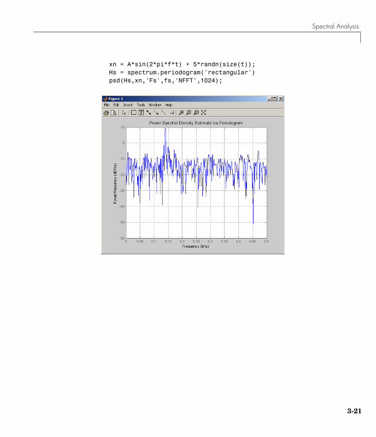
Spectral Analysis
xn = A*sin(2*pi*f*t) + 5*randn(size(t));Hs = spectrum.periodogram('rectangular')psd(Hs,xn,'Fs',fs,'NFFT',1024);
3-21
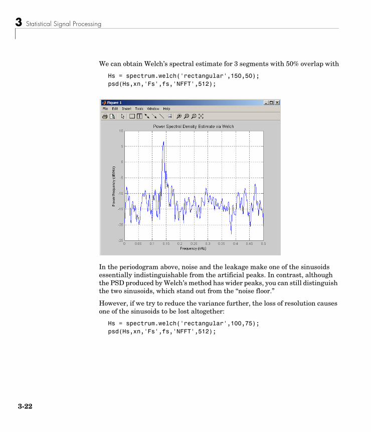
3 Statistical Signal Processing
3-2
We can obtain Welch’s spectral estimate for 3 segments with 50% overlap with
Hs = spectrum.welch('rectangular',150,50);psd(Hs,xn,'Fs',fs,'NFFT',512);
In the periodogram above, noise and the leakage make one of the sinusoids essentially indistinguishable from the artificial peaks. In contrast, although the PSD produced by Welch’s method has wider peaks, you can still distinguish the two sinusoids, which stand out from the “noise floor.”
However, if we try to reduce the variance further, the loss of resolution causes one of the sinusoids to be lost altogether:
Hs = spectrum.welch('rectangular',100,75);psd(Hs,xn,'Fs',fs,'NFFT',512);
2
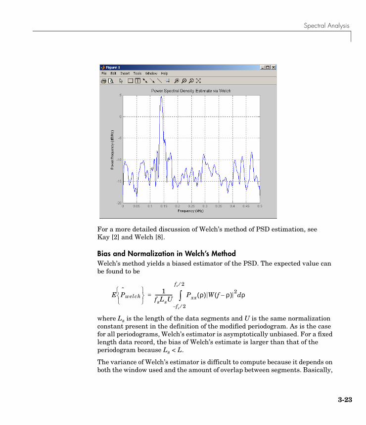
Spectral Analysis
For a more detailed discussion of Welch’s method of PSD estimation, see Kay [2] and Welch [8].
Bias and Normalization in Welch’s MethodWelch’s method yields a biased estimator of the PSD. The expected value can be found to be
where Ls is the length of the data segments and U is the same normalization constant present in the definition of the modified periodogram. As is the case for all periodograms, Welch’s estimator is asymptotically unbiased. For a fixed length data record, the bias of Welch’s estimate is larger than that of the periodogram because Ls < L.
The variance of Welch’s estimator is difficult to compute because it depends on both the window used and the amount of overlap between segments. Basically,
E Pˆ
welch 1
fsLsU---------------- Pxx ρ( ) W f ρ–( ) 2 ρd
fs 2⁄–
fs 2⁄
∫=
3-23
3 Statistical Signal Processing
3-2
the variance is inversely proportional to the number of segments whose modified periodograms are being averaged.
Multitaper MethodThe periodogram can be interpreted as filtering a length L signal, xL[n], through a filter bank (a set of filters in parallel) of L FIR bandpass filters. The 3 dB bandwidth of each of these bandpass filters can be shown to be approximately equal to fs / L. The magnitude response of each one of these bandpass filters resembles that of the rectangular window discussed in “Spectral Leakage” on page 3-12. The periodogram can thus be viewed as a computation of the power of each filtered signal (i.e., the output of each bandpass filter) that uses just one sample of each filtered signal and assumes that the PSD of xL[n] is constant over the bandwidth of each bandpass filter.
As the length of the signal increases, the bandwidth of each bandpass filter decreases, making it a more selective filter, and improving the approximation of constant PSD over the bandwidth of the filter. This provides another interpretation of why the PSD estimate of the periodogram improves as the length of the signal increases. However, there are two factors apparent from this standpoint that compromise the accuracy of the periodogram estimate. First, the rectangular window yields a poor bandpass filter. Second, the computation of the power at the output of each bandpass filter relies on a single sample of the output signal, producing a very crude approximation.
Welch’s method can be given a similar interpretation in terms of a filter bank. In Welch’s implementation, several samples are used to compute the output power, resulting in reduced variance of the estimate. On the other hand, the bandwidth of each bandpass filter is larger than that corresponding to the periodogram method, which results in a loss of resolution. The filter bank model thus provides a new interpretation of the compromise between variance and resolution.
Thompson’s multitaper method (MTM) builds on these results to provide an improved PSD estimate. Instead of using bandpass filters that are essentially rectangular windows (as in the periodogram method), the MTM method uses a bank of optimal bandpass filters to compute the estimate. These optimal FIR filters are derived from a set of sequences known as discrete prolate spheroidal sequences (DPSSs, also known as Slepian sequences).
In addition, the MTM method provides a time-bandwidth parameter with which to balance the variance and resolution. This parameter is given by the
4
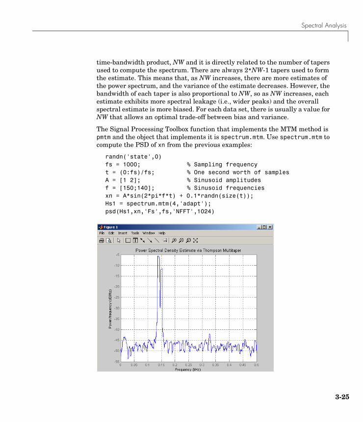
Spectral Analysis
time-bandwidth product, NW and it is directly related to the number of tapers used to compute the spectrum. There are always 2*NW-1 tapers used to form the estimate. This means that, as NW increases, there are more estimates of the power spectrum, and the variance of the estimate decreases. However, the bandwidth of each taper is also proportional to NW, so as NW increases, each estimate exhibits more spectral leakage (i.e., wider peaks) and the overall spectral estimate is more biased. For each data set, there is usually a value for NW that allows an optimal trade-off between bias and variance.
The Signal Processing Toolbox function that implements the MTM method is pmtm and the object that implements it is spectrum.mtm. Use spectrum.mtm to compute the PSD of xn from the previous examples:
randn('state',0)fs = 1000; % Sampling frequencyt = (0:fs)/fs; % One second worth of samplesA = [1 2]; % Sinusoid amplitudesf = [150;140]; % Sinusoid frequenciesxn = A*sin(2*pi*f*t) + 0.1*randn(size(t));Hs1 = spectrum.mtm(4,'adapt');psd(Hs1,xn,'Fs',fs,'NFFT',1024)
3-25
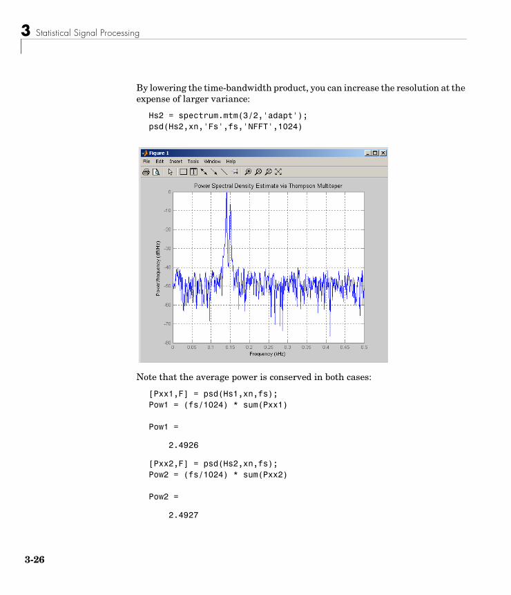
3 Statistical Signal Processing
3-2
By lowering the time-bandwidth product, you can increase the resolution at the expense of larger variance:
Hs2 = spectrum.mtm(3/2,'adapt');psd(Hs2,xn,'Fs',fs,'NFFT',1024)
Note that the average power is conserved in both cases:
[Pxx1,F] = psd(Hs1,xn,fs);Pow1 = (fs/1024) * sum(Pxx1)
Pow1 =
2.4926
[Pxx2,F] = psd(Hs2,xn,fs);Pow2 = (fs/1024) * sum(Pxx2)
Pow2 =
2.4927
6
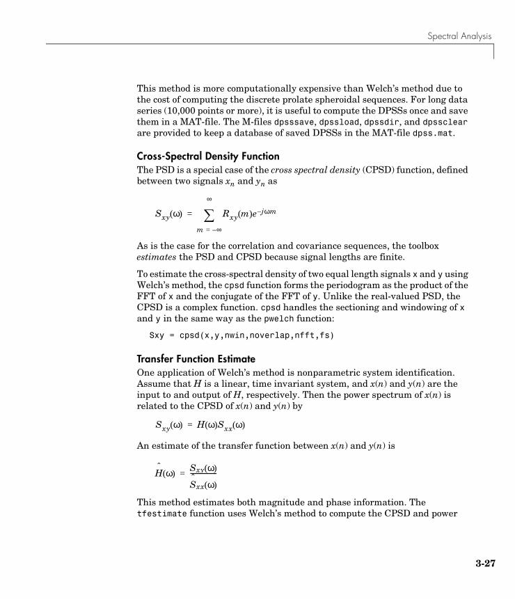
Spectral Analysis
This method is more computationally expensive than Welch’s method due to the cost of computing the discrete prolate spheroidal sequences. For long data series (10,000 points or more), it is useful to compute the DPSSs once and save them in a MAT-file. The M-files dpsssave, dpssload, dpssdir, and dpssclear are provided to keep a database of saved DPSSs in the MAT-file dpss.mat.
Cross-Spectral Density FunctionThe PSD is a special case of the cross spectral density (CPSD) function, defined between two signals xn and yn as
As is the case for the correlation and covariance sequences, the toolbox estimates the PSD and CPSD because signal lengths are finite.
To estimate the cross-spectral density of two equal length signals x and y using Welch’s method, the cpsd function forms the periodogram as the product of the FFT of x and the conjugate of the FFT of y. Unlike the real-valued PSD, the CPSD is a complex function. cpsd handles the sectioning and windowing of x and y in the same way as the pwelch function:
Sxy = cpsd(x,y,nwin,noverlap,nfft,fs)
Transfer Function EstimateOne application of Welch’s method is nonparametric system identification. Assume that H is a linear, time invariant system, and x(n) and y(n) are the input to and output of H, respectively. Then the power spectrum of x(n) is related to the CPSD of x(n) and y(n) by
An estimate of the transfer function between x(n) and y(n) is
This method estimates both magnitude and phase information. The tfestimate function uses Welch’s method to compute the CPSD and power
Sxy ω( ) Rxy m( )e jωm–
m ∞–=
∞
∑=
Sxy ω( ) H ω( )Sxx ω( )=
Hˆ
ω( )Sˆ
xy ω( )
Sˆ
xx ω( )-----------------=
3-27
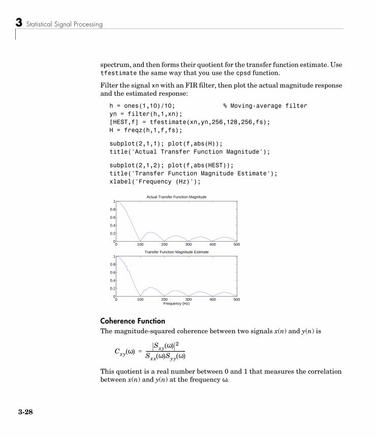
3 Statistical Signal Processing
3-2
spectrum, and then forms their quotient for the transfer function estimate. Use tfestimate the same way that you use the cpsd function.
Filter the signal xn with an FIR filter, then plot the actual magnitude response and the estimated response:
h = ones(1,10)/10; % Moving-average filteryn = filter(h,1,xn);[HEST,f] = tfestimate(xn,yn,256,128,256,fs);H = freqz(h,1,f,fs);
subplot(2,1,1); plot(f,abs(H)); title('Actual Transfer Function Magnitude');
subplot(2,1,2); plot(f,abs(HEST));title('Transfer Function Magnitude Estimate'); xlabel('Frequency (Hz)');
Coherence FunctionThe magnitude-squared coherence between two signals x(n) and y(n) is
This quotient is a real number between 0 and 1 that measures the correlation between x(n) and y(n) at the frequency ω.
0 100 200 300 400 5000
0.2
0.4
0.6
0.8
1Actual Transfer Function Magnitude
0 100 200 300 400 5000
0.2
0.4
0.6
0.8
1Transfer Function Magnitude Estimate
Frequency (Hz)
Cxy ω( )Sxy ω( ) 2
Sxx ω( )Syy ω( )-----------------------------------=
8
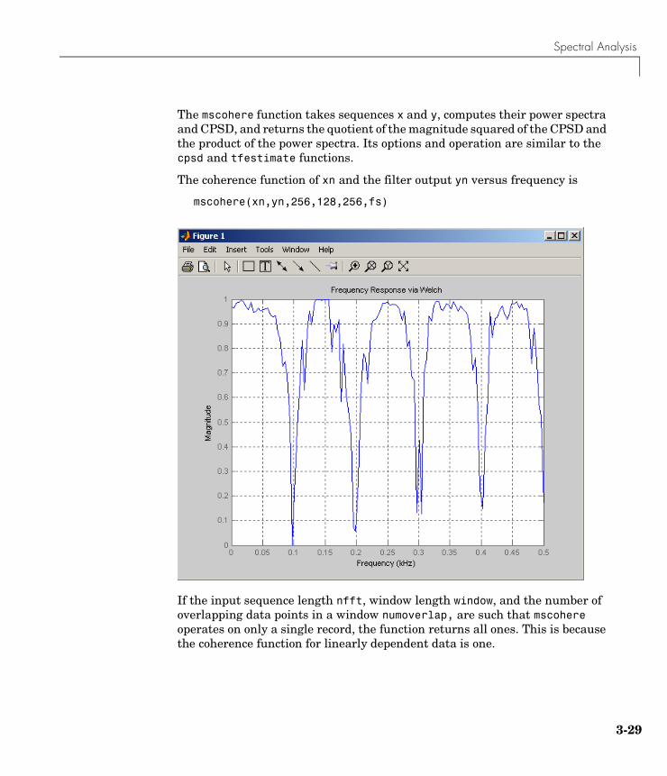
Spectral Analysis
The mscohere function takes sequences x and y, computes their power spectra and CPSD, and returns the quotient of the magnitude squared of the CPSD and the product of the power spectra. Its options and operation are similar to the cpsd and tfestimate functions.
The coherence function of xn and the filter output yn versus frequency is
mscohere(xn,yn,256,128,256,fs)
If the input sequence length nfft, window length window, and the number of overlapping data points in a window numoverlap, are such that mscohere operates on only a single record, the function returns all ones. This is because the coherence function for linearly dependent data is one.
3-29
3 Statistical Signal Processing
3-3
The following example shows how to use spectral analysis functions to compute the coherence:
randn('state',0) fs = 1000; % Sampling frequency t = (0:fs)/fs; % One second worth of samples A = [1 2]; % Sinusoid amplitudesf = [150;140]; % Sinusoid frequencies xn = A*sin(2*pi*f*t) + 0.1*randn(size(t));h = ones(1,10)/10; % Moving average filter yn = filter(h,1,xn);
% Parameters common to both CPSD and MSCOHERE:nfft = 256;noverlap = 128;nwin = hanning(256);CxyCohere = mscohere(xn,yn,nwin,noverlap,nfft,fs);
% Compute the PSDs using Welch s method, which is similar to the% MSCOHERE function[Sxx,F] = pwelch(xn,nwin,noverlap,nfft,fs);[Syy,F] = pwelch(yn,nwin,noverlap,nfft,fs);
% Convert one-sided PSDs to Power SpectrumsSxx = [Sxx(1); (Sxx(2:end-1)/2); Sxx(end)].*fs;Syy = [Syy(1); (Syy(2:end-1)/2); Syy(end)].*fs;
% Call CPSD function with similar arguments as the MSCOHERE function% from above.[Sxy,F] = cpsd(xn,yn,nwin,noverlap,nfft,fs);Cxy = (abs(Sxy).^2)./(Sxx.*Syy);plot(1:length(Cxy), [CxyCohere Cxy]); % Compare the estimates
0
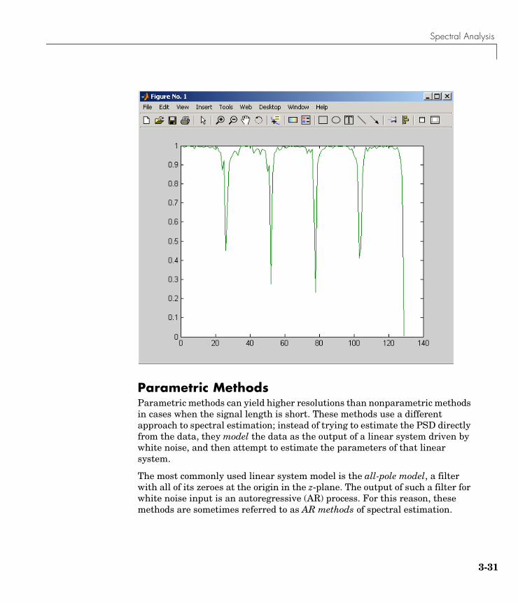
Spectral Analysis
Parametric MethodsParametric methods can yield higher resolutions than nonparametric methods in cases when the signal length is short. These methods use a different approach to spectral estimation; instead of trying to estimate the PSD directly from the data, they model the data as the output of a linear system driven by white noise, and then attempt to estimate the parameters of that linear system.
The most commonly used linear system model is the all-pole model, a filter with all of its zeroes at the origin in the z-plane. The output of such a filter for white noise input is an autoregressive (AR) process. For this reason, these methods are sometimes referred to as AR methods of spectral estimation.
3-31
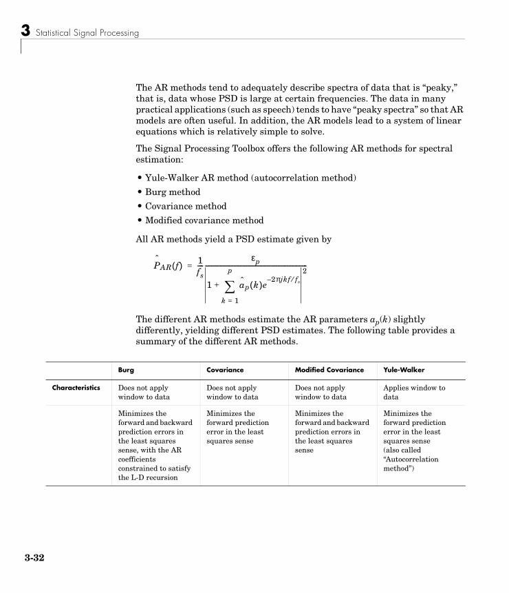
3 Statistical Signal Processing
3-3
The AR methods tend to adequately describe spectra of data that is “peaky,” that is, data whose PSD is large at certain frequencies. The data in many practical applications (such as speech) tends to have “peaky spectra” so that AR models are often useful. In addition, the AR models lead to a system of linear equations which is relatively simple to solve.
The Signal Processing Toolbox offers the following AR methods for spectral estimation:
• Yule-Walker AR method (autocorrelation method)
• Burg method
• Covariance method
• Modified covariance method
All AR methods yield a PSD estimate given by
The different AR methods estimate the AR parameters ap(k) slightly differently, yielding different PSD estimates. The following table provides a summary of the different AR methods.
Pˆ
AR f( ) 1fs----
εp
1 ap k( )e2πjkf– fs⁄
k 1=
p
∑+
2-------------------------------------------------------------------=
Burg Covariance Modified Covariance Yule-Walker
Characteristics Does not apply window to data
Does not apply window to data
Does not apply window to data
Applies window to data
Minimizes the forward and backward prediction errors in the least squares sense, with the AR coefficients constrained to satisfy the L-D recursion
Minimizes the forward prediction error in the least squares sense
Minimizes the forward and backward prediction errors in the least squares sense
Minimizes the forward prediction error in the least squares sense(also called “Autocorrelation method”)
2
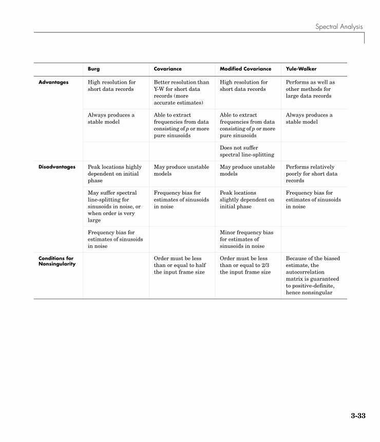
Spectral Analysis
Advantages High resolution for short data records
Better resolution than Y-W for short data records (more accurate estimates)
High resolution for short data records
Performs as well as other methods for large data records
Always produces a stable model
Able to extract frequencies from data consisting of p or more pure sinusoids
Able to extract frequencies from data consisting of p or more pure sinusoids
Always produces a stable model
Does not suffer spectral line-splitting
Disadvantages Peak locations highly dependent on initial phase
May produce unstable models
May produce unstable models
Performs relatively poorly for short data records
May suffer spectral line-splitting for sinusoids in noise, or when order is very large
Frequency bias for estimates of sinusoids in noise
Peak locations slightly dependent on initial phase
Frequency bias for estimates of sinusoids in noise
Frequency bias for estimates of sinusoids in noise
Minor frequency bias for estimates of sinusoids in noise
Conditions for Nonsingularity
Order must be less than or equal to half the input frame size
Order must be less than or equal to 2/3 the input frame size
Because of the biased estimate, the autocorrelation matrix is guaranteed to positive-definite, hence nonsingular
Burg Covariance Modified Covariance Yule-Walker
3-33
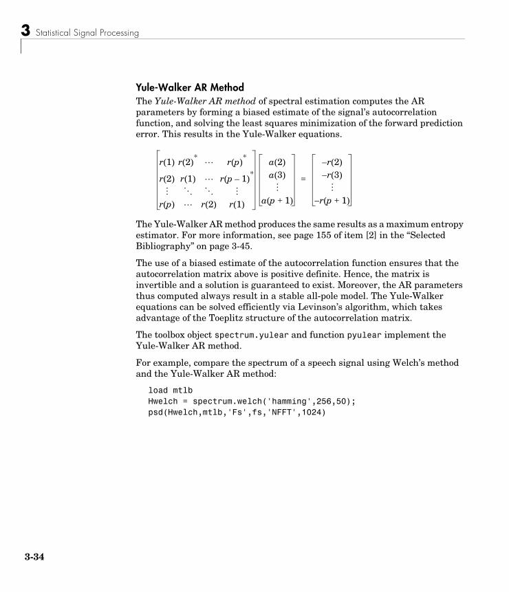
3 Statistical Signal Processing
3-3
Yule-Walker AR MethodThe Yule-Walker AR method of spectral estimation computes the AR parameters by forming a biased estimate of the signal’s autocorrelation function, and solving the least squares minimization of the forward prediction error. This results in the Yule-Walker equations.
The Yule-Walker AR method produces the same results as a maximum entropy estimator. For more information, see page 155 of item [2] in the “Selected Bibliography” on page 3-45.
The use of a biased estimate of the autocorrelation function ensures that the autocorrelation matrix above is positive definite. Hence, the matrix is invertible and a solution is guaranteed to exist. Moreover, the AR parameters thus computed always result in a stable all-pole model. The Yule-Walker equations can be solved efficiently via Levinson’s algorithm, which takes advantage of the Toeplitz structure of the autocorrelation matrix.
The toolbox object spectrum.yulear and function pyulear implement the Yule-Walker AR method.
For example, compare the spectrum of a speech signal using Welch’s method and the Yule-Walker AR method:
load mtlbHwelch = spectrum.welch('hamming',256,50);psd(Hwelch,mtlb,'Fs',fs,'NFFT',1024)
r 1( ) r 2( )* r p( )
*
r 2( ) r 1( ) r p 1–( )*
r p( ) r 2( ) r 1( )
a 2( )
a 3( )
a p 1+( )
r 2( )–
r 3( )–
r p 1+( )–
=
4
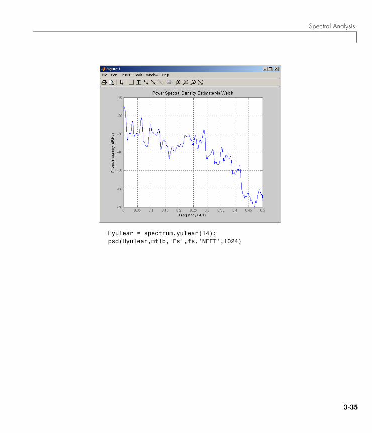
Spectral Analysis
Hyulear = spectrum.yulear(14);psd(Hyulear,mtlb,'Fs',fs,'NFFT',1024)
3-35
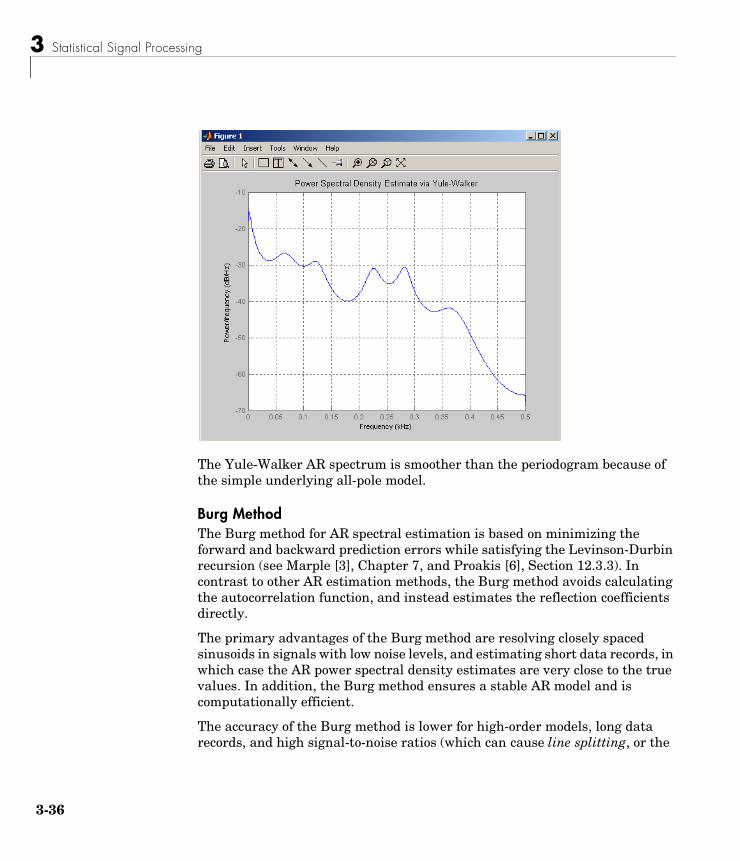
3 Statistical Signal Processing
3-3
The Yule-Walker AR spectrum is smoother than the periodogram because of the simple underlying all-pole model.
Burg MethodThe Burg method for AR spectral estimation is based on minimizing the forward and backward prediction errors while satisfying the Levinson-Durbin recursion (see Marple [3], Chapter 7, and Proakis [6], Section 12.3.3). In contrast to other AR estimation methods, the Burg method avoids calculating the autocorrelation function, and instead estimates the reflection coefficients directly.
The primary advantages of the Burg method are resolving closely spaced sinusoids in signals with low noise levels, and estimating short data records, in which case the AR power spectral density estimates are very close to the true values. In addition, the Burg method ensures a stable AR model and is computationally efficient.
The accuracy of the Burg method is lower for high-order models, long data records, and high signal-to-noise ratios (which can cause line splitting, or the
6
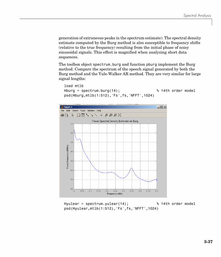
Spectral Analysis
generation of extraneous peaks in the spectrum estimate). The spectral density estimate computed by the Burg method is also susceptible to frequency shifts (relative to the true frequency) resulting from the initial phase of noisy sinusoidal signals. This effect is magnified when analyzing short data sequences.
The toolbox object spectrum.burg and function pburg implement the Burg method. Compare the spectrum of the speech signal generated by both the Burg method and the Yule-Walker AR method. They are very similar for large signal lengths:
load mtlbHburg = spectrum.burg(14); % 14th order modelpsd(Hburg,mtlb(1:512),'Fs',fs,'NFFT',1024)
Hyulear = spectrum.yulear(14); % 14th order modelpsd(Hyulear,mtlb(1:512),'Fs',fs,'NFFT',1024)
3-37
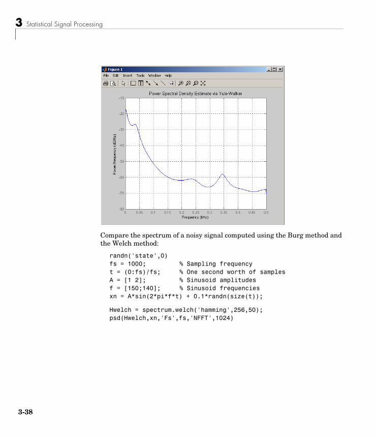
3 Statistical Signal Processing
3-3
Compare the spectrum of a noisy signal computed using the Burg method and the Welch method:
randn('state',0)fs = 1000; % Sampling frequencyt = (0:fs)/fs; % One second worth of samplesA = [1 2]; % Sinusoid amplitudesf = [150;140]; % Sinusoid frequenciesxn = A*sin(2*pi*f*t) + 0.1*randn(size(t));
Hwelch = spectrum.welch('hamming',256,50);psd(Hwelch,xn,'Fs',fs,'NFFT',1024)
8
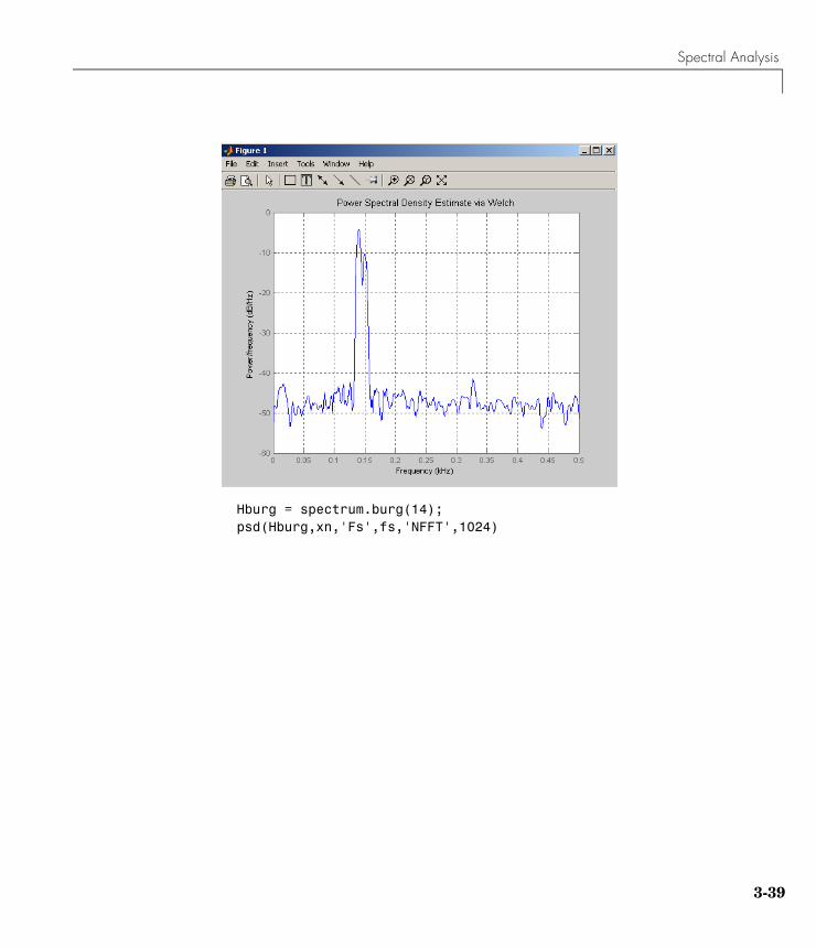
Spectral Analysis
Hburg = spectrum.burg(14);psd(Hburg,xn,'Fs',fs,'NFFT',1024)
3-39
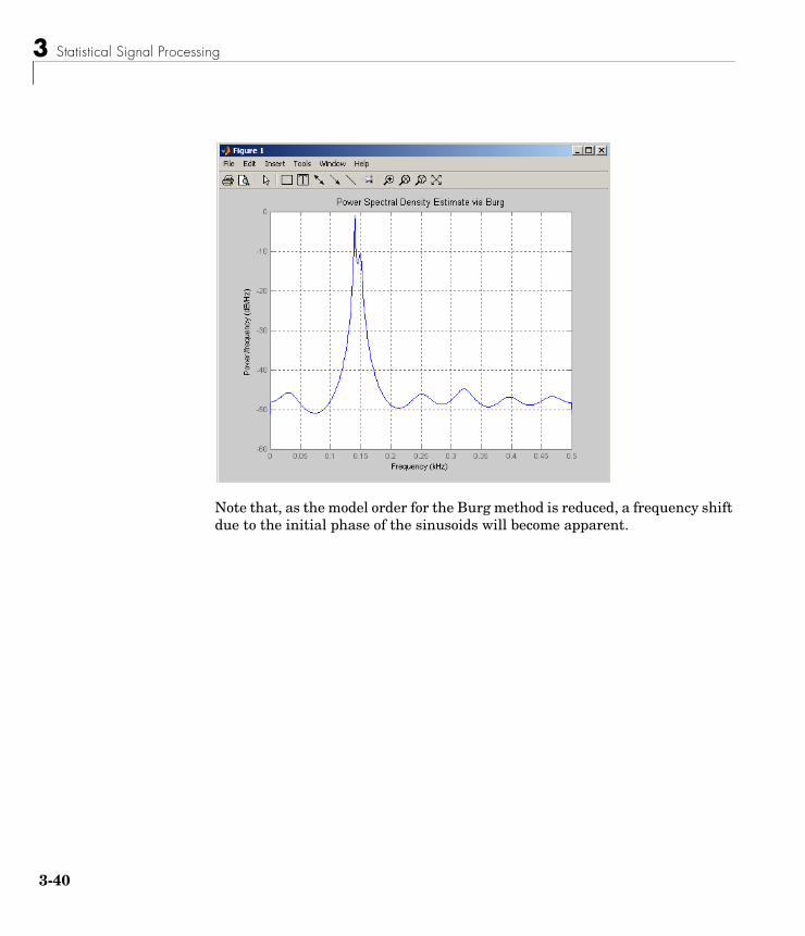
3 Statistical Signal Processing
3-4
Note that, as the model order for the Burg method is reduced, a frequency shift due to the initial phase of the sinusoids will become apparent.
0
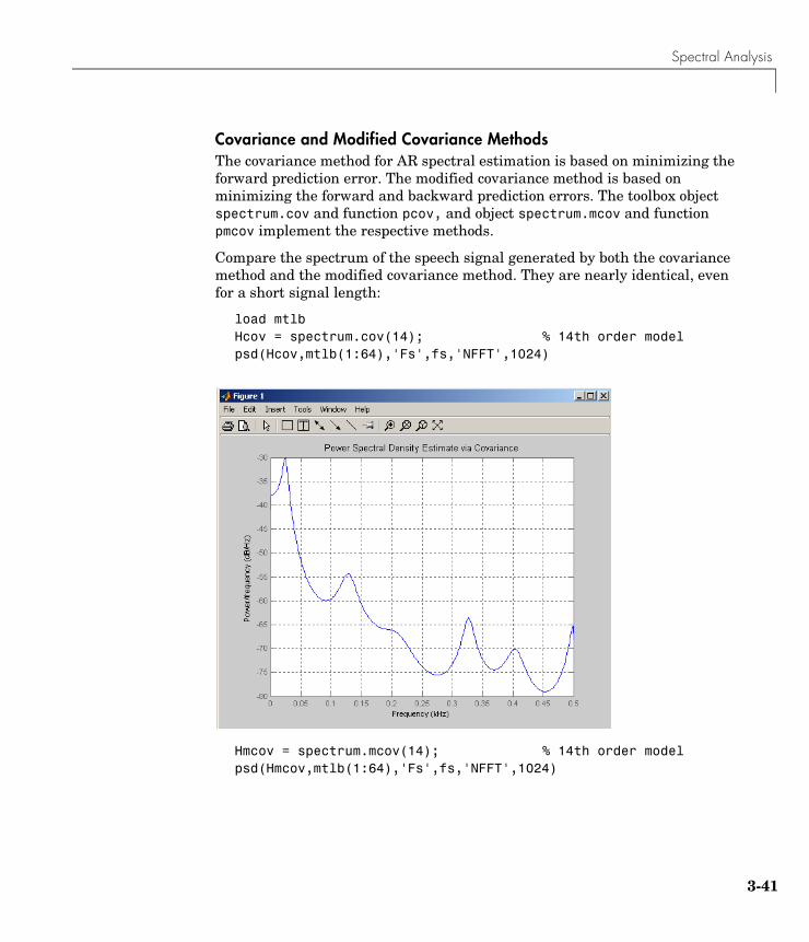
Spectral Analysis
Covariance and Modified Covariance MethodsThe covariance method for AR spectral estimation is based on minimizing the forward prediction error. The modified covariance method is based on minimizing the forward and backward prediction errors. The toolbox object spectrum.cov and function pcov, and object spectrum.mcov and function pmcov implement the respective methods.
Compare the spectrum of the speech signal generated by both the covariance method and the modified covariance method. They are nearly identical, even for a short signal length:
load mtlbHcov = spectrum.cov(14); % 14th order modelpsd(Hcov,mtlb(1:64),'Fs',fs,'NFFT',1024)
Hmcov = spectrum.mcov(14); % 14th order modelpsd(Hmcov,mtlb(1:64),'Fs',fs,'NFFT',1024)
3-41
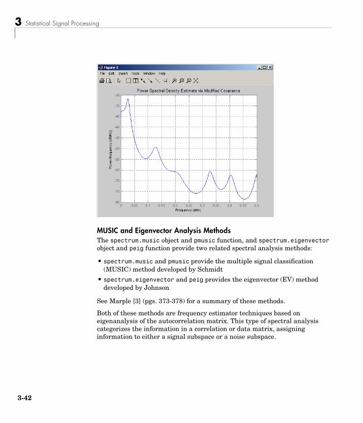
3 Statistical Signal Processing
3-4
MUSIC and Eigenvector Analysis MethodsThe spectrum.music object and pmusic function, and spectrum.eigenvector object and peig function provide two related spectral analysis methods:
• spectrum.music and pmusic provide the multiple signal classification (MUSIC) method developed by Schmidt
• spectrum.eigenvector and peig provides the eigenvector (EV) method developed by Johnson
See Marple [3] (pgs. 373-378) for a summary of these methods.
Both of these methods are frequency estimator techniques based on eigenanalysis of the autocorrelation matrix. This type of spectral analysis categorizes the information in a correlation or data matrix, assigning information to either a signal subspace or a noise subspace.
2
Spectral Analysis
Eigenanalysis OverviewConsider a number of complex sinusoids embedded in white noise. You can write the autocorrelation matrix R for this system as the sum of the signal autocorrelation matrix (S) and the noise autocorrelation matrix (W):
There is a close relationship between the eigenvectors of the signal autocorrelation matrix and the signal and noise subspaces. The eigenvectors v of S span the same signal subspace as the signal vectors. If the system contains M complex sinusoids and the order of the autocorrelation matrix is p, eigenvectors vM+1 through vp+1 span the noise subspace of the autocorrelation matrix.
Frequency Estimator Functions. To generate their frequency estimates, eigenanalysis methods calculate functions of the vectors in the signal and noise subspaces. Both the MUSIC and EV techniques choose a function that goes to infinity (denominator goes to zero) at one of the sinusoidal frequencies in the input signal. Using digital technology, the resulting estimate has sharp peaks at the frequencies of interest; this means that there might not be infinity values in the vectors.
The MUSIC estimate is given by the formula
where N is the size of the eigenvectors and e(f) is a vector of complex sinusoids.
v represents the eigenvectors of the input signal’s correlation matrix; vk is the kth eigenvector. H is the conjugate transpose operator. The eigenvectors used in the sum correspond to the smallest eigenvalues and span the noise subspace (p is the size of the signal subspace).
The expression is equivalent to a Fourier transform (the vector e(f) consists of complex exponentials). This form is useful for numeric computation because the FFT can be computed for each vk and then the squared magnitudes can be summed.
R S W+=
Pmusic f( )1
eH f( ) vkvkH
k p 1+=
N
∑
e f( )
---------------------------------------------------------------- 1
vkHe f( ) 2
k p 1+=
N
∑
-------------------------------------------= =
e f( ) 1 exp j2πf( ) exp j2πf 2⋅( ) exp j2πf 4⋅( ) … exp j2πf n 1–( )⋅( )[ ] H=
vkHe f( )
3-43
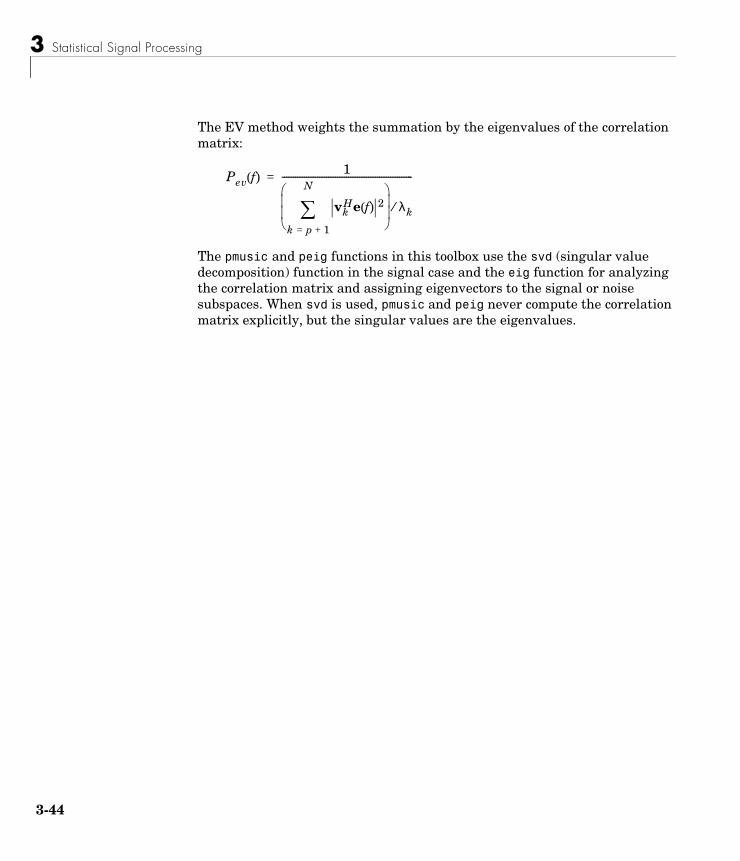
3 Statistical Signal Processing
3-4
The EV method weights the summation by the eigenvalues of the correlation matrix:
The pmusic and peig functions in this toolbox use the svd (singular value decomposition) function in the signal case and the eig function for analyzing the correlation matrix and assigning eigenvectors to the signal or noise subspaces. When svd is used, pmusic and peig never compute the correlation matrix explicitly, but the singular values are the eigenvalues.
Pev f( )1
vkHe f( ) 2
k p 1+=
N
∑
λk⁄
-----------------------------------------------------------=
4

Selected Bibliography
Selected Bibliography[1] Hayes, M.H. Statistical Digital Signal Processing and Modeling. New York: John Wiley & Sons, 1996.
[2] Kay, S.M. Modern Spectral Estimation. Englewood Cliffs, NJ: Prentice Hall, 1988.
[3] Marple, S.L. Digital Spectral Analysis. Englewood Cliffs, NJ: Prentice Hall, 1987.
[4] Orfanidis, S.J. Introduction to Signal Processing. Upper Saddle River, NJ: Prentice Hall, 1996.
[5] Percival, D.B., and A.T. Walden. Spectral Analysis for Physical Applications: Multitaper and Conventional Univariate Techniques. Cambridge: Cambridge University Press, 1993.
[6] Proakis, J.G., and D.G. Manolakis. Digital Signal Processing: Principles, Algorithms, and Applications. Englewood Cliffs, NJ: Prentice Hall, 1996.
[7] Stoica, P., and R. Moses. Introduction to Spectral Analysis. Upper Saddle River, NJ: Prentice Hall, 1997.
[8] Welch, P.D. “The Use of Fast Fourier Transform for the Estimation of Power Spectra: A Method Based on Time Averaging Over Short, Modified Periodograms.” IEEE Trans. Audio Electroacoust. Vol. AU-15 (June 1967). Pgs. 70-73.
3-45

3 Statistical Signal Processing
3-4
6
4
Special Topics
The following chapter describes specialized techniques and applications provided in the Signal Processing Toolbox.
Windows (p. 4-2) Window background information and toolbox functions and GUIs
Parametric Modeling (p. 4-17) Mathemical techniques for modeling systems
Resampling (p. 4-28) Functions for resampling a signal at a different sampling rate
Cepstrum Analysis (p. 4-30) Functions for performing cepstrum analysis
FFT-Based Time-Frequency Analysis (p. 4-34)
Spectrograms
Median Filtering (p. 4-35) Applying a sliding window to a sequence
Communications Applications (p. 4-36) Functions for communications simulations
Deconvolution (p. 4-42) Deconvolution information
Specialized Transforms (p. 4-43) Chirp Z, discrete-cosine, and Hilbert transforms
Selected Bibliography (p. 4-49) Sources of additional information
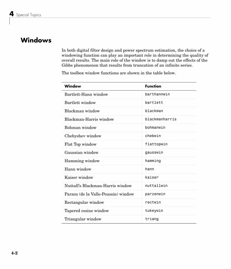
4 Special Topics
4-2
WindowsIn both digital filter design and power spectrum estimation, the choice of a windowing function can play an important role in determining the quality of overall results. The main role of the window is to damp out the effects of the Gibbs phenomenon that results from truncation of an infinite series.
The toolbox window functions are shown in the table below.
Window Function
Bartlett-Hann window barthannwin
Bartlett window bartlett
Blackman window blackman
Blackman-Harris window blackmanharris
Bohman window bohmanwin
Chebyshev window chebwin
Flat Top window flattopwin
Gaussian window gausswin
Hamming window hamming
Hann window hann
Kaiser window kaiser
Nuttall’s Blackman-Harris window nuttallwin
Parzen (de la Valle-Poussin) window parzenwin
Rectangular window rectwin
Tapered cosine window tukeywin
Triangular window triang

Windows
Graphical User Interface ToolsTwo graphical user interface tools are provided for working with windows in the Signal Processing toolbox:
• Window Design and Analysis Tool (wintool)
• Window Visualization Tool (wvtool)
Basic ShapesThe basic window is the rectangular window, a vector of ones of the appropriate length. A rectangular window of length 50 is
n = 50;w = rectwin(n);
This toolbox stores windows in column vectors by convention, so an equivalent expression is
w = ones(50,1);
To use the Window Design and Analysis Tool to create this window, type
wintool
wintool opens with a default Hamming window. In the Current Window Information panel, set Type = Rectangular and Length = 50 and then press Apply.
4-3
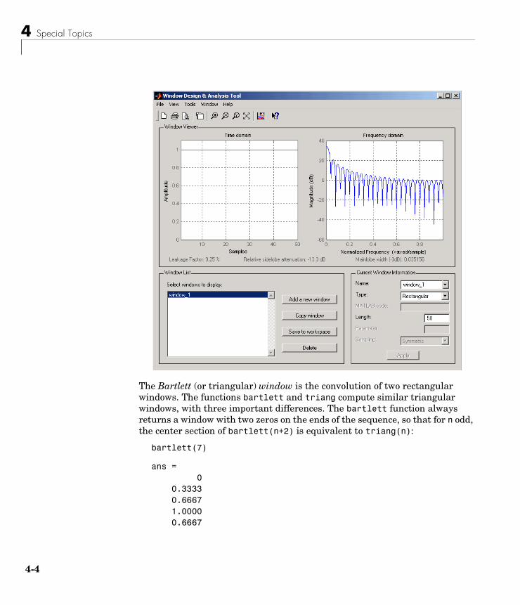
4 Special Topics
4-4
The Bartlett (or triangular) window is the convolution of two rectangular windows. The functions bartlett and triang compute similar triangular windows, with three important differences. The bartlett function always returns a window with two zeros on the ends of the sequence, so that for n odd, the center section of bartlett(n+2) is equivalent to triang(n):
bartlett(7)
ans = 0 0.3333 0.6667 1.0000 0.6667
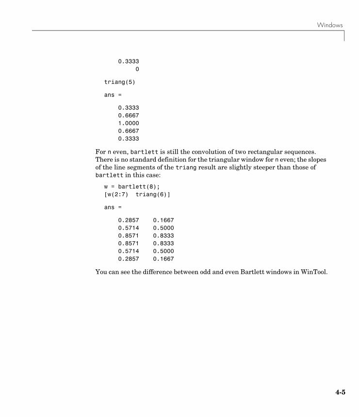
Windows
0.3333 0
triang(5)
ans =
0.3333 0.6667 1.0000 0.6667 0.3333
For n even, bartlett is still the convolution of two rectangular sequences. There is no standard definition for the triangular window for n even; the slopes of the line segments of the triang result are slightly steeper than those of bartlett in this case:
w = bartlett(8); [w(2:7) triang(6)]
ans =
0.2857 0.1667 0.5714 0.5000 0.8571 0.8333 0.8571 0.8333 0.5714 0.5000 0.2857 0.1667
You can see the difference between odd and even Bartlett windows in WinTool.
4-5
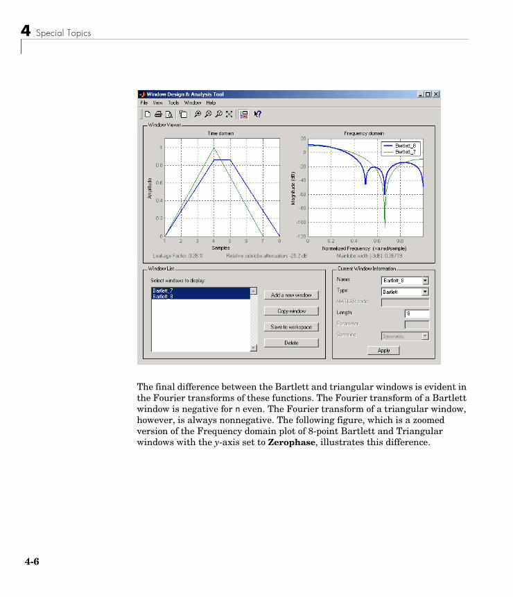
4 Special Topics
4-6
The final difference between the Bartlett and triangular windows is evident in the Fourier transforms of these functions. The Fourier transform of a Bartlett window is negative for n even. The Fourier transform of a triangular window, however, is always nonnegative. The following figure, which is a zoomed version of the Frequency domain plot of 8-point Bartlett and Triangular windows with the y-axis set to Zerophase, illustrates this difference.
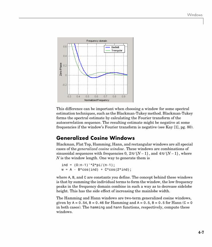
Windows
This difference can be important when choosing a window for some spectral estimation techniques, such as the Blackman-Tukey method. Blackman-Tukey forms the spectral estimate by calculating the Fourier transform of the autocorrelation sequence. The resulting estimate might be negative at some frequencies if the window’s Fourier transform is negative (see Kay [1], pg. 80).
Generalized Cosine WindowsBlackman, Flat Top, Hamming, Hann, and rectangular windows are all special cases of the generalized cosine window. These windows are combinations of sinusoidal sequences with frequencies 0, , and , where N is the window length. One way to generate them is
ind = (0:n-1)'*2*pi/(n-1);w = A - B*cos(ind) + C*cos(2*ind);
where A, B, and C are constants you define. The concept behind these windows is that by summing the individual terms to form the window, the low frequency peaks in the frequency domain combine in such a way as to decrease sidelobe height. This has the side effect of increasing the mainlobe width.
The Hamming and Hann windows are two-term generalized cosine windows, given by A = 0.54, B = 0.46 for Hamming and A = 0.5, B = 0.5 for Hann (C = 0 in both cases). The hamming and hann functions, respectively, compute these windows.
2π N 1–( )⁄ 4π N 1–( )⁄
4-7
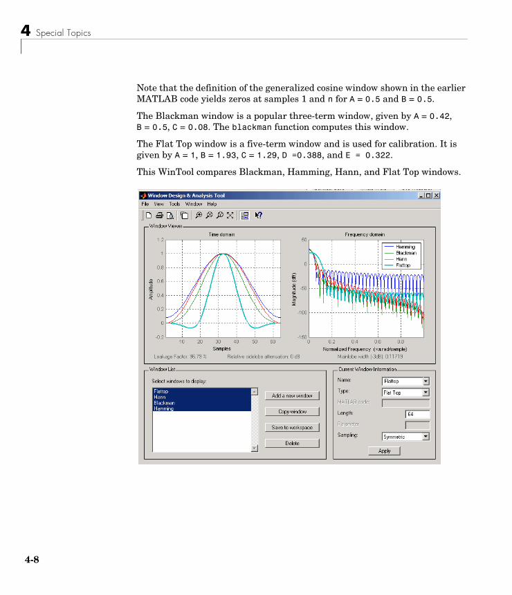
4 Special Topics
4-8
Note that the definition of the generalized cosine window shown in the earlier MATLAB code yields zeros at samples 1 and n for A = 0.5 and B = 0.5.
The Blackman window is a popular three-term window, given by A = 0.42, B = 0.5, C = 0.08. The blackman function computes this window.
The Flat Top window is a five-term window and is used for calibration. It is given by A = 1, B = 1.93, C = 1.29, D =0.388, and E = 0.322.
This WinTool compares Blackman, Hamming, Hann, and Flat Top windows.
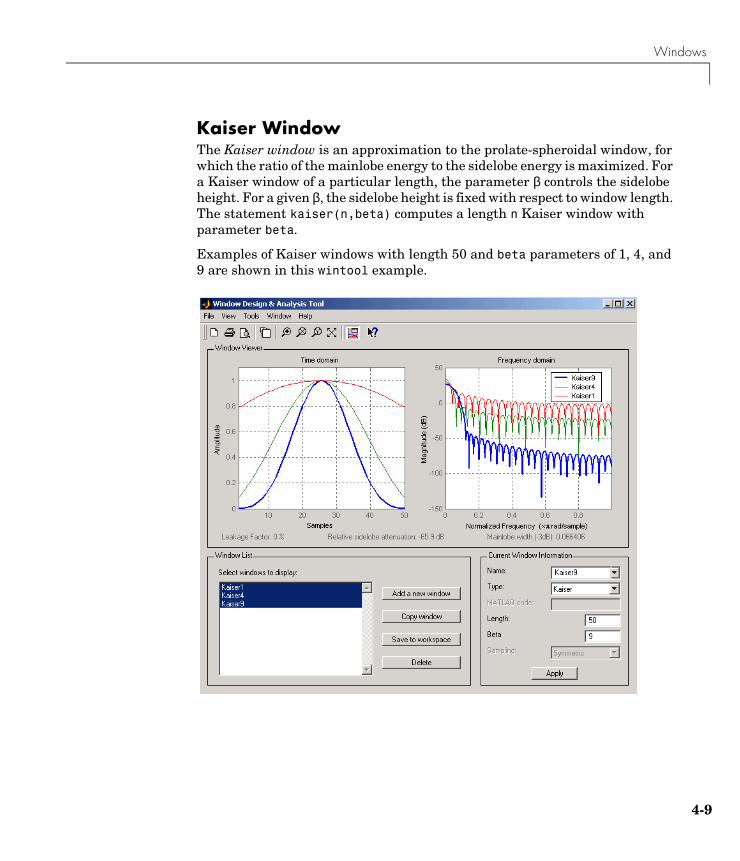
Windows
Kaiser WindowThe Kaiser window is an approximation to the prolate-spheroidal window, for which the ratio of the mainlobe energy to the sidelobe energy is maximized. For a Kaiser window of a particular length, the parameter β controls the sidelobe height. For a given β, the sidelobe height is fixed with respect to window length. The statement kaiser(n,beta) computes a length n Kaiser window with parameter beta.
Examples of Kaiser windows with length 50 and beta parameters of 1, 4, and 9 are shown in this wintool example.
4-9
4 Special Topics
4-1
To create these Kaiser windows using the MATLAB command line,
n = 50;w1 = kaiser(n,1);w2 = kaiser(n,4);w3 = kaiser(n,9);[W1,f] = freqz(w1/sum(w1),1,512,2);[W2,f] = freqz(w2/sum(w2),1,512,2);[W3,f] = freqz(w3/sum(w3),1,512,2);plot(f,20*log10(abs([W1 W2 W3]))); grid;legend('beta = 1','beta = 4','beta = 9',3)
As β increases, the sidelobe height decreases and the mainlobe width increases. This wintool shows how the sidelobe height stays the same for a fixed β parameter as the length is varied.
0
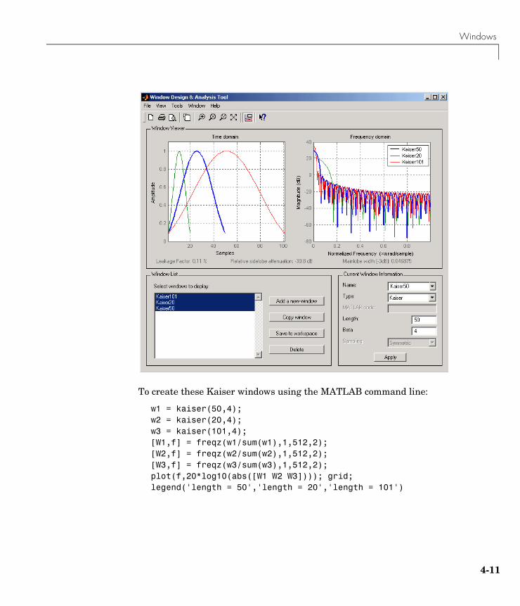
Windows
To create these Kaiser windows using the MATLAB command line:
w1 = kaiser(50,4);w2 = kaiser(20,4);w3 = kaiser(101,4);[W1,f] = freqz(w1/sum(w1),1,512,2);[W2,f] = freqz(w2/sum(w2),1,512,2);[W3,f] = freqz(w3/sum(w3),1,512,2);plot(f,20*log10(abs([W1 W2 W3]))); grid;legend('length = 50','length = 20','length = 101')
4-11
4 Special Topics
4-1
Kaiser Windows in FIR DesignThere are two design formulas that can help you design FIR filters to meet a set of filter specifications using a Kaiser window. To achieve a sidelobe height of −α dB, the beta parameter is
For a transition width of ∆ω rad/s, use the length
Filters designed using these heuristics will meet the specifications approximately, but you should verify this. To design a lowpass filter with cutoff frequency rad/s, transition width rad/s, and 40 dB of attenuation in the stopband, try
[n,wn,beta] = kaiserord([0.4 0.6]*pi,[1 0],[0.01 0.01],2*pi);h = fir1(n,wn,kaiser(n+1,beta),'noscale');
The kaiserord function estimates the filter order, cutoff frequency, and Kaiser window beta parameter needed to meet a given set of frequency domain specifications.
The ripple in the passband is roughly the same as the ripple in the stopband. As you can see from the frequency response, this filter nearly meets the specifications:
fvtool(h,1);
β0.1102 α 8.7–( ), α 50>0.5842 α 21–( )0.4 0.07886 α 21–( )+ , 50 α 21≥ ≥0, α 21<
=
n α 8–2.285 ω∆----------------------- 1+=
0.5π 0.2π
2
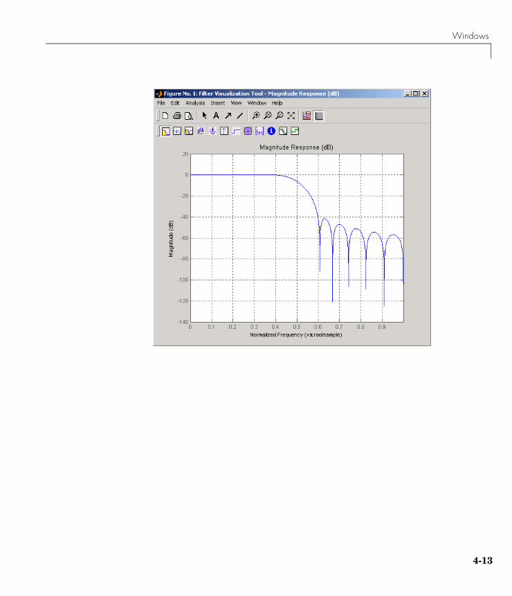
Windows
4-13
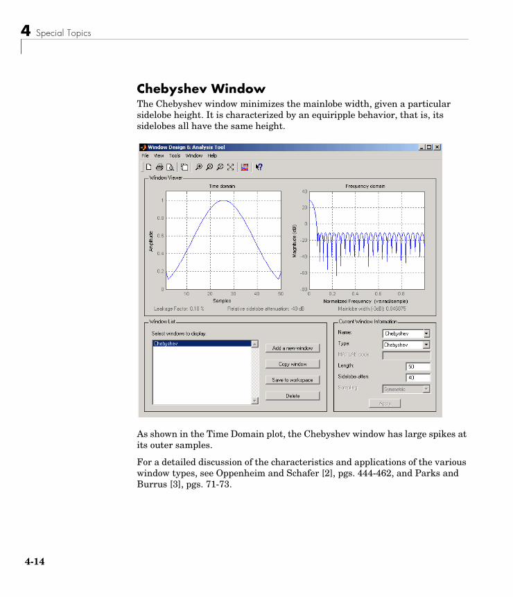
4 Special Topics
4-1
Chebyshev WindowThe Chebyshev window minimizes the mainlobe width, given a particular sidelobe height. It is characterized by an equiripple behavior, that is, its sidelobes all have the same height.
As shown in the Time Domain plot, the Chebyshev window has large spikes at its outer samples.
For a detailed discussion of the characteristics and applications of the various window types, see Oppenheim and Schafer [2], pgs. 444-462, and Parks and Burrus [3], pgs. 71-73.
4
Parametric Modeling
Parametric ModelingParametric modeling techniques find the parameters for a mathematical model describing a signal, system, or process. These techniques use known information about the system to determine the model. Applications for parametric modeling include speech and music synthesis, data compression, high-resolution spectral estimation, communications, manufacturing, and simulation.
The toolbox parametric modeling functions operate with the rational transfer function model. Given appropriate information about an unknown system (impulse or frequency response data, or input and output sequences), these functions find the coefficients of a linear system that models the system.
One important application of the parametric modeling functions is in the design of filters that have a prescribed time or frequency response. These functions provide a data-oriented alternative to the IIR and FIR filter design functions discussed in Chapter 2, “Filter Design and Implementation.”
4-15
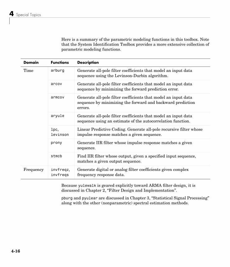
4 Special Topics
4-1
Here is a summary of the parametric modeling functions in this toolbox. Note that the System Identification Toolbox provides a more extensive collection of parametric modeling functions.
Because yulewalk is geared explicitly toward ARMA filter design, it is discussed in Chapter 2, “Filter Design and Implementation”.
pburg and pyulear are discussed in Chapter 3, “Statistical Signal Processing” along with the other (nonparametric) spectral estimation methods.
Domain Functions Description
Time arburg Generate all-pole filter coefficients that model an input data sequence using the Levinson-Durbin algorithm.
arcov Generate all-pole filter coefficients that model an input data sequence by minimizing the forward prediction error.
armcov Generate all-pole filter coefficients that model an input data sequence by minimizing the forward and backward prediction errors.
aryule Generate all-pole filter coefficients that model an input data sequence using an estimate of the autocorrelation function.
lpc, levinson
Linear Predictive Coding. Generate all-pole recursive filter whose impulse response matches a given sequence.
prony Generate IIR filter whose impulse response matches a given sequence.
stmcb Find IIR filter whose output, given a specified input sequence, matches a given output sequence.
Frequency invfreqz, invfreqs
Generate digital or analog filter coefficients given complex frequency response data.
6
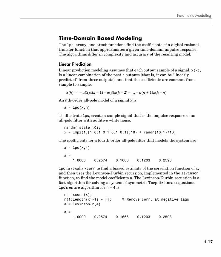
Parametric Modeling
Time-Domain Based ModelingThe lpc, prony, and stmcb functions find the coefficients of a digital rational transfer function that approximates a given time-domain impulse response. The algorithms differ in complexity and accuracy of the resulting model.
Linear PredictionLinear prediction modeling assumes that each output sample of a signal, x(k), is a linear combination of the past n outputs (that is, it can be “linearly predicted” from these outputs), and that the coefficients are constant from sample to sample:
An nth-order all-pole model of a signal x is
a = lpc(x,n)
To illustrate lpc, create a sample signal that is the impulse response of an all-pole filter with additive white noise:
randn('state',0);x = impz(1,[1 0.1 0.1 0.1 0.1],10) + randn(10,1)/10;
The coefficients for a fourth-order all-pole filter that models the system are
a = lpc(x,4)
a = 1.0000 0.2574 0.1666 0.1203 0.2598
lpc first calls xcorr to find a biased estimate of the correlation function of x, and then uses the Levinson-Durbin recursion, implemented in the levinson function, to find the model coefficients a. The Levinson-Durbin recursion is a fast algorithm for solving a system of symmetric Toeplitz linear equations. lpc’s entire algorithm for n = 4 is
r = xcorr(x);r(1:length(x)-1) = []; % Remove corr. at negative lagsa = levinson(r,4)
a = 1.0000 0.2574 0.1666 0.1203 0.2598
x k( ) a 2( )x k 1–( )– a 3( )x k 2–( )– …– a n 1+( )x k n–( )–=
4-17
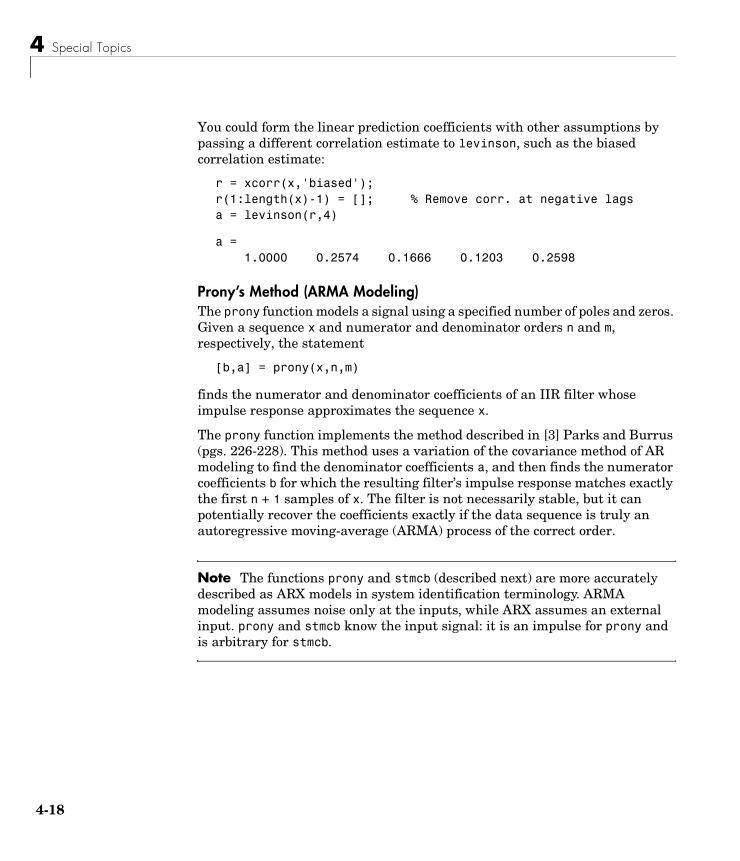
4 Special Topics
4-1
You could form the linear prediction coefficients with other assumptions by passing a different correlation estimate to levinson, such as the biased correlation estimate:
r = xcorr(x,'biased');r(1:length(x)-1) = []; % Remove corr. at negative lagsa = levinson(r,4)
a = 1.0000 0.2574 0.1666 0.1203 0.2598
Prony’s Method (ARMA Modeling)The prony function models a signal using a specified number of poles and zeros. Given a sequence x and numerator and denominator orders n and m, respectively, the statement
[b,a] = prony(x,n,m)
finds the numerator and denominator coefficients of an IIR filter whose impulse response approximates the sequence x.
The prony function implements the method described in [3] Parks and Burrus (pgs. 226-228). This method uses a variation of the covariance method of AR modeling to find the denominator coefficients a, and then finds the numerator coefficients b for which the resulting filter’s impulse response matches exactly the first n + 1 samples of x. The filter is not necessarily stable, but it can potentially recover the coefficients exactly if the data sequence is truly an autoregressive moving-average (ARMA) process of the correct order.
Note The functions prony and stmcb (described next) are more accurately described as ARX models in system identification terminology. ARMA modeling assumes noise only at the inputs, while ARX assumes an external input. prony and stmcb know the input signal: it is an impulse for prony and is arbitrary for stmcb.
8
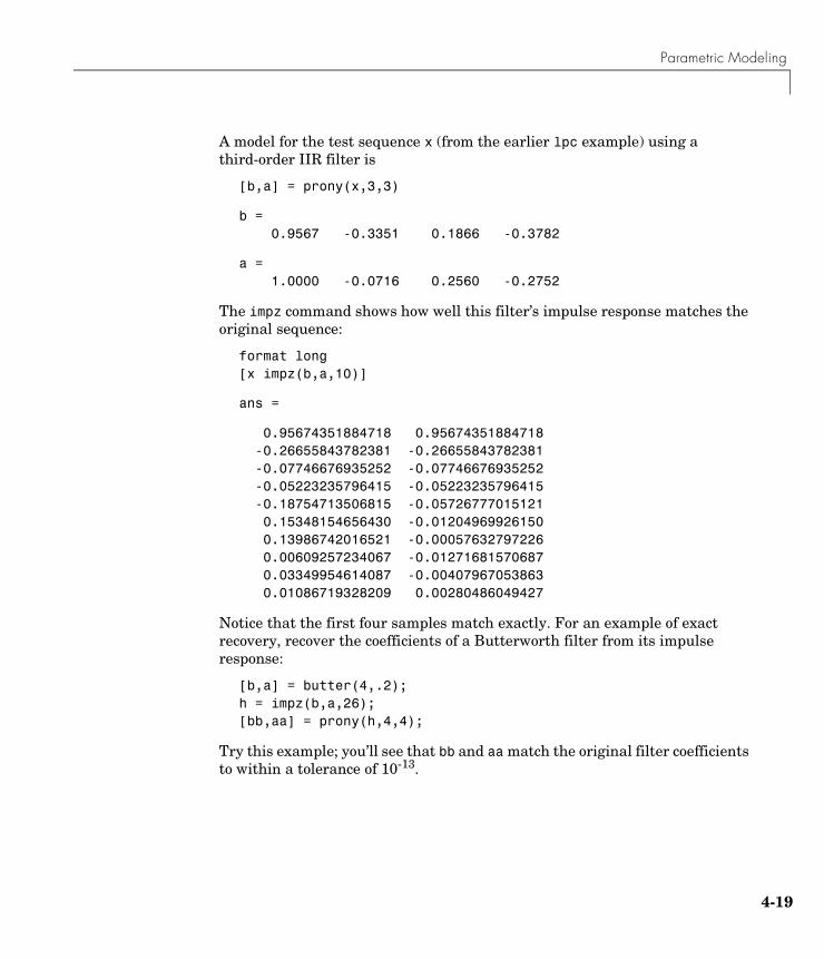
Parametric Modeling
A model for the test sequence x (from the earlier lpc example) using a third-order IIR filter is
[b,a] = prony(x,3,3)
b = 0.9567 -0.3351 0.1866 -0.3782
a = 1.0000 -0.0716 0.2560 -0.2752
The impz command shows how well this filter’s impulse response matches the original sequence:
format long[x impz(b,a,10)]
ans =
0.95674351884718 0.95674351884718 -0.26655843782381 -0.26655843782381 -0.07746676935252 -0.07746676935252 -0.05223235796415 -0.05223235796415 -0.18754713506815 -0.05726777015121 0.15348154656430 -0.01204969926150 0.13986742016521 -0.00057632797226 0.00609257234067 -0.01271681570687 0.03349954614087 -0.00407967053863 0.01086719328209 0.00280486049427
Notice that the first four samples match exactly. For an example of exact recovery, recover the coefficients of a Butterworth filter from its impulse response:
[b,a] = butter(4,.2);h = impz(b,a,26);[bb,aa] = prony(h,4,4);
Try this example; you’ll see that bb and aa match the original filter coefficients to within a tolerance of 10-13.
4-19
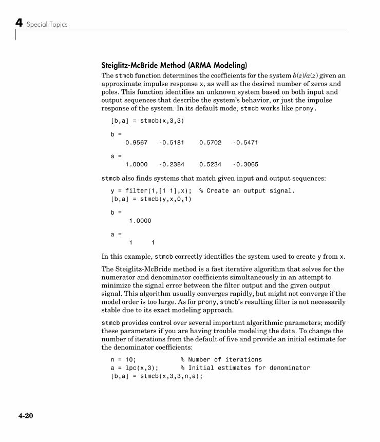
4 Special Topics
4-2
Steiglitz-McBride Method (ARMA Modeling)The stmcb function determines the coefficients for the system b(z)/a(z) given an approximate impulse response x, as well as the desired number of zeros and poles. This function identifies an unknown system based on both input and output sequences that describe the system’s behavior, or just the impulse response of the system. In its default mode, stmcb works like prony.
[b,a] = stmcb(x,3,3)
b = 0.9567 -0.5181 0.5702 -0.5471
a = 1.0000 -0.2384 0.5234 -0.3065
stmcb also finds systems that match given input and output sequences:
y = filter(1,[1 1],x); % Create an output signal.[b,a] = stmcb(y,x,0,1)
b = 1.0000
a = 1 1
In this example, stmcb correctly identifies the system used to create y from x.
The Steiglitz-McBride method is a fast iterative algorithm that solves for the numerator and denominator coefficients simultaneously in an attempt to minimize the signal error between the filter output and the given output signal. This algorithm usually converges rapidly, but might not converge if the model order is too large. As for prony, stmcb’s resulting filter is not necessarily stable due to its exact modeling approach.
stmcb provides control over several important algorithmic parameters; modify these parameters if you are having trouble modeling the data. To change the number of iterations from the default of five and provide an initial estimate for the denominator coefficients:
n = 10; % Number of iterationsa = lpc(x,3); % Initial estimates for denominator[b,a] = stmcb(x,3,3,n,a);
0
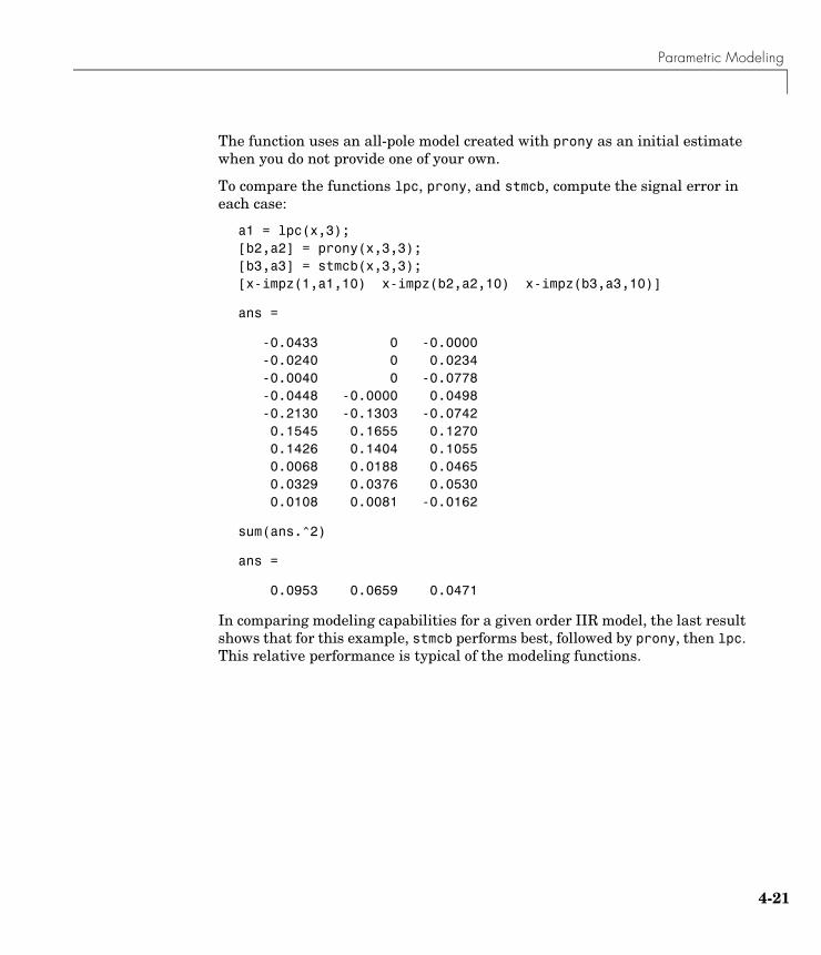
Parametric Modeling
The function uses an all-pole model created with prony as an initial estimate when you do not provide one of your own.
To compare the functions lpc, prony, and stmcb, compute the signal error in each case:
a1 = lpc(x,3);[b2,a2] = prony(x,3,3);[b3,a3] = stmcb(x,3,3);[x-impz(1,a1,10) x-impz(b2,a2,10) x-impz(b3,a3,10)]
ans =
-0.0433 0 -0.0000 -0.0240 0 0.0234 -0.0040 0 -0.0778 -0.0448 -0.0000 0.0498 -0.2130 -0.1303 -0.0742 0.1545 0.1655 0.1270 0.1426 0.1404 0.1055 0.0068 0.0188 0.0465 0.0329 0.0376 0.0530 0.0108 0.0081 -0.0162
sum(ans.^2)
ans =
0.0953 0.0659 0.0471
In comparing modeling capabilities for a given order IIR model, the last result shows that for this example, stmcb performs best, followed by prony, then lpc. This relative performance is typical of the modeling functions.
4-21
4 Special Topics
4-2
Frequency-Domain Based ModelingThe invfreqs and invfreqz functions implement the inverse operations of freqs and freqz; they find an analog or digital transfer function of a specified order that matches a given complex frequency response. Though the following examples demonstrate invfreqz, the discussion also applies to invfreqs.
To recover the original filter coefficients from the frequency response of a simple digital filter:
[b,a] = butter(4,0.4) % Design Butterworth lowpass
b = 0.0466 0.1863 0.2795 0.1863 0.0466
a = 1.0000 -0.7821 0.6800 -0.1827 0.0301
[h,w] = freqz(b,a,64); % Compute frequency response[b4,a4] = invfreqz(h,w,4,4) % Model: n = 4, m = 4
b4 =
0.0466 0.1863 0.2795 0.1863 0.0466
a4 =
1.0000 -0.7821 0.6800 -0.1827 0.0301
The vector of frequencies w has the units in rad/sample, and the frequencies need not be equally spaced. invfreqz finds a filter of any order to fit the frequency data; a third-order example is
[b4,a4] = invfreqz(h,w,3,3) % Find third-order IIR
b4 =
0.0464 0.1785 0.2446 0.1276
a4 =
1.0000 -0.9502 0.7382 -0.2006
Both invfreqs and invfreqz design filters with real coefficients; for a data point at positive frequency f, the functions fit the frequency response at both f and -f.
2
Parametric Modeling
By default invfreqz uses an equation error method to identify the best model from the data. This finds b and a in
by creating a system of linear equations and solving them with the MATLAB \ operator. Here A(w(k)) and B(w(k)) are the Fourier transforms of the polynomials a and b respectively at the frequency w(k), and n is the number of frequency points (the length of h and w). wt(k) weights the error relative to the error at different frequencies. The syntax
invfreqz(h,w,n,m,wt)
includes a weighting vector. In this mode, the filter resulting from invfreqz is not guaranteed to be stable.
invfreqz provides a superior (“output-error”) algorithm that solves the direct problem of minimizing the weighted sum of the squared error between the actual frequency response points and the desired response
To use this algorithm, specify a parameter for the iteration count after the weight vector parameter:
wt = ones(size(w)); % Create unity weighting vector[b30,a30] = invfreqz(h,w,3,3,wt,30) % 30 iterations
b30 =
0.0464 0.1829 0.2572 0.1549
a30 =
1.0000 -0.8664 0.6630 -0.1614
The resulting filter is always stable.
minb a,
wt k( ) h k( )A w k( )( ) B w k( )( )– 2
k 1=
n
∑
minb a,
wt k( ) h k( )B w k( )( )A w k( )( )--------------------–
2
k 1=
n
∑
4-23
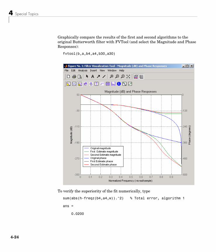
4 Special Topics
4-2
Graphically compare the results of the first and second algorithms to the original Butterworth filter with FVTool (and select the Magnitude and Phase Responses):
fvtool(b,a,b4,a4,b30,a30)
To verify the superiority of the fit numerically, type
sum(abs(h-freqz(b4,a4,w)).^2) % Total error, algorithm 1
ans =
0.0200
4

Parametric Modeling
sum(abs(h-freqz(b30,a30,w)).^2) % Total error, algorithm 2
ans =
0.0096
4-25
4 Special Topics
4-2
ResamplingThe toolbox provides a number of functions that resample a signal at a higher or lower rate.
The resample function changes the sampling rate for a sequence to any rate that is a ratio of two integers. The basic syntax for resample is
y = resample(x,p,q)
where the function resamples the sequence x at p/q times the original sampling rate. The length of the result y is p/q times the length of x.
One resampling application is the conversion of digitized audio signals from one sampling rate to another, such as from 48 kHz (the digital audio tape standard) to 44.1 kHz (the compact disc standard).
The example file contains a length 4001 vector of speech sampled at 7418 Hz:
clearload mtlbwhos
Name Size Bytes Class Fs 1x1 8 double array mtlb 4001x1 32008 double array
Grand total is 4002 elements using 32016 bytes
Fs
Operation Function
Apply FIR filter with resampling upfirdn
Cubic spline interpolation spline
Decimation decimate
Interpolation interp
Other 1-D interpolation interp1
Resample at new rate resample
6
Resampling
Fs = 7418
To play this speech signal on a workstation that can only play sound at 8192 Hz, use the rat function to find integers p and q that yield the correct resampling factor:
[p,q] = rat(8192/Fs,0.0001)
p = 127q = 115
Since p/q*Fs = 8192.05 Hz, the tolerance of 0.0001 is acceptable; to resample the signal at very close to 8192 Hz:
y = resample(mtlb,p,q);
resample applies a lowpass filter to the input sequence to prevent aliasing during resampling. It designs this filter using the firls function with a Kaiser window. The syntax
resample(x,p,q,l,beta)
controls the filter’s length and the beta parameter of the Kaiser window. Alternatively, use the function intfilt to design an interpolation filter b and use it with
resample(x,p,q,b)
The decimate and interp functions do the same thing as resample with p = 1 and q = 1, respectively. These functions provide different anti-alias filtering options, and they incur a slight signal delay due to filtering. The interp function is significantly less efficient than the resample function with q = 1.
The toolbox also contains a function, upfirdn, that applies an FIR filter to an input sequence and outputs the filtered sequence at a sample rate different than its original. See “Multirate Filter Bank Implementation” on page 1-20.
The standard MATLAB environment contains a function, spline, that works with irregularly spaced data. The MATLAB function interp1 performs interpolation, or table lookup, using various methods including linear and cubic interpolation.
4-27
4 Special Topics
4-2
Cepstrum AnalysisCepstrum analysis is a nonlinear signal processing technique with a variety of applications in areas such as speech and image processing. The Signal Processing Toolbox provides three functions for cepstrum analysis.
The complex cepstrum for a sequence x is calculated by finding the complex natural logarithm of the Fourier transform of x, then the inverse Fourier transform of the resulting sequence.
The toolbox function cceps performs this operation, estimating the complex cepstrum for an input sequence. It returns a real sequence the same size as the input sequence:
xhat = cceps(x)
The complex cepstrum transformation is central to the theory and application of homomorphic systems, that is, systems that obey certain general rules of superposition. See Oppenheim and Schafer [2] for a discussion of the complex cepstrum and homomorphic transformations, with details on speech processing applications.
Try using cceps in an echo detection application. First, create a 45 Hz sine wave sampled at 100 Hz:
t = 0:0.01:1.27;s1 = sin(2*pi*45*t);
Add an echo of the signal, with half the amplitude, 0.2 seconds after the beginning of the signal.
Operation Function
Complex cepstrum cceps
Inverse complex cepstrum icceps
Real cepstrum rceps
x 12π------ X ejω( )[ ]log ejωn ωd
π–
π
∫=
8
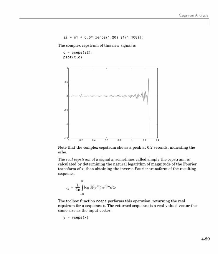
Cepstrum Analysis
s2 = s1 + 0.5*[zeros(1,20) s1(1:108)];
The complex cepstrum of this new signal is
c = cceps(s2);plot(t,c)
Note that the complex cepstrum shows a peak at 0.2 seconds, indicating the echo.
The real cepstrum of a signal x, sometimes called simply the cepstrum, is calculated by determining the natural logarithm of magnitude of the Fourier transform of x, then obtaining the inverse Fourier transform of the resulting sequence.
The toolbox function rceps performs this operation, returning the real cepstrum for a sequence x. The returned sequence is a real-valued vector the same size as the input vector:
y = rceps(x)
0 0.2 0.4 0.6 0.8 1 1.2 1.4-1.5
-1
-0.5
0
0.5
1
cx1
2π------ X ejω( )log ejωn ωd
π–
π
∫=
4-29
4 Special Topics
4-3
By definition, you cannot reconstruct the original sequence from its real cepstrum transformation, as the real cepstrum is based only on the magnitude of the Fourier transform for the sequence (see Oppenheim and Schafer [2]). The rceps function, however, can reconstruct a minimum-phase version of the original sequence by applying a windowing function in the cepstral domain. To obtain both the real cepstrum and the minimum phase reconstruction for a sequence, use
[y,ym] = rceps(x)
where y is the real cepstrum and ym is the minimum phase reconstruction of x.
Inverse Complex CepstrumTo invert the complex cepstrum, use the icceps function. Inversion is complicated by the fact that the cceps function performs a data dependent phase modification so that the unwrapped phase of its input is continuous at zero frequency. The phase modification is equivalent to an integer delay. This delay term is returned by cceps if you ask for a second output. For example:
x = 1:10;[xh,nd] = cceps(x)
xh = Columns 1 through 7 2.2428 -0.0420 -0.0210 0.0045 0.0366 0.0788 0.1386 Columns 8 through 10 0.2327 0.4114 0.9249
nd = 1
0
Cepstrum Analysis
To invert the complex cepstrum, use icceps with the original delay parameter:
icceps(xh,nd)
ans = Columns 1 through 7 1.0000 2.0000 3.0000 4.0000 5.0000 6.0000 7.0000 Columns 8 through 10 8.0000 9.0000 10.0000
Note With any modification of the complex cepstrum, the original delay term may no longer be valid. Use the icceps function with care.
4-31
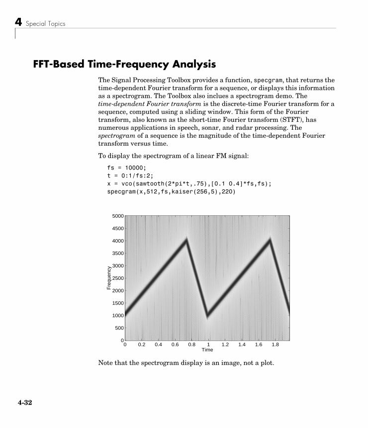
4 Special Topics
4-3
FFT-Based Time-Frequency AnalysisThe Signal Processing Toolbox provides a function, specgram, that returns the time-dependent Fourier transform for a sequence, or displays this information as a spectrogram. The Toolbox also inclues a spectrogram demo. The time-dependent Fourier transform is the discrete-time Fourier transform for a sequence, computed using a sliding window. This form of the Fourier transform, also known as the short-time Fourier transform (STFT), has numerous applications in speech, sonar, and radar processing. The spectrogram of a sequence is the magnitude of the time-dependent Fourier transform versus time.
To display the spectrogram of a linear FM signal:
fs = 10000;t = 0:1/fs:2;x = vco(sawtooth(2*pi*t,.75),[0.1 0.4]*fs,fs);specgram(x,512,fs,kaiser(256,5),220)
Note that the spectrogram display is an image, not a plot.
Time
Fre
quen
cy
0 0.2 0.4 0.6 0.8 1 1.2 1.4 1.6 1.80
500
1000
1500
2000
2500
3000
3500
4000
4500
5000
2
Median Filtering
Median FilteringThe function medfilt1 implements one-dimensional median filtering, a nonlinear technique that applies a sliding window to a sequence. The median filter replaces the center value in the window with the median value of all the points within the window [4]. In computing this median, medfilt1 assumes zeros beyond the input points.
When the number of elements n in the window is even, medfilt1 sorts the numbers, then takes the average of the (n-1)/2 and (n-1)/2 + 1 elements.
Two simple examples with fourth- and third-order median filters are
medfilt1([4 3 5 2 8 9 1],4)
ans =
1.500 3.500 3.500 4.000 6.500 5.000 4.500
medfilt1([4 3 5 2 8 9 1],3)
ans =
3 4 3 5 8 8 1
See the medfilt2 function in the Image Processing Toolbox documentation for information on two-dimensional median filtering.
4-33
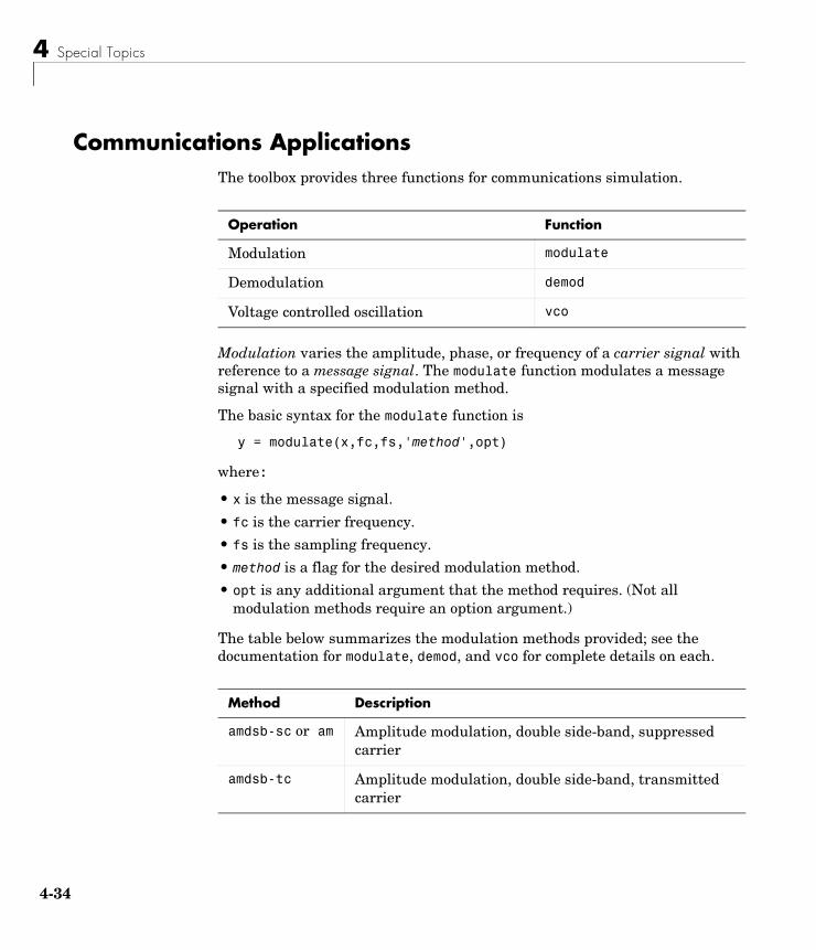
4 Special Topics
4-3
Communications ApplicationsThe toolbox provides three functions for communications simulation.
Modulation varies the amplitude, phase, or frequency of a carrier signal with reference to a message signal. The modulate function modulates a message signal with a specified modulation method.
The basic syntax for the modulate function is
y = modulate(x,fc,fs,'method',opt)
where:
• x is the message signal.
• fc is the carrier frequency.
• fs is the sampling frequency.
• method is a flag for the desired modulation method.
• opt is any additional argument that the method requires. (Not all modulation methods require an option argument.)
The table below summarizes the modulation methods provided; see the documentation for modulate, demod, and vco for complete details on each.
Operation Function
Modulation modulate
Demodulation demod
Voltage controlled oscillation vco
Method Description
amdsb-sc or am Amplitude modulation, double side-band, suppressed carrier
amdsb-tc Amplitude modulation, double side-band, transmitted carrier
4
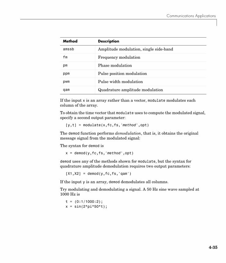
Communications Applications
If the input x is an array rather than a vector, modulate modulates each column of the array.
To obtain the time vector that modulate uses to compute the modulated signal, specify a second output parameter:
[y,t] = modulate(x,fc,fs,'method',opt)
The demod function performs demodulation, that is, it obtains the original message signal from the modulated signal:
The syntax for demod is
x = demod(y,fc,fs,'method',opt)
demod uses any of the methods shown for modulate, but the syntax for quadrature amplitude demodulation requires two output parameters:
[X1,X2] = demod(y,fc,fs,'qam')
If the input y is an array, demod demodulates all columns.
Try modulating and demodulating a signal. A 50 Hz sine wave sampled at 1000 Hz is
t = (0:1/1000:2);x = sin(2*pi*50*t);
amssb Amplitude modulation, single side-band
fm Frequency modulation
pm Phase modulation
ppm Pulse position modulation
pwm Pulse width modulation
qam Quadrature amplitude modulation
Method Description
4-35
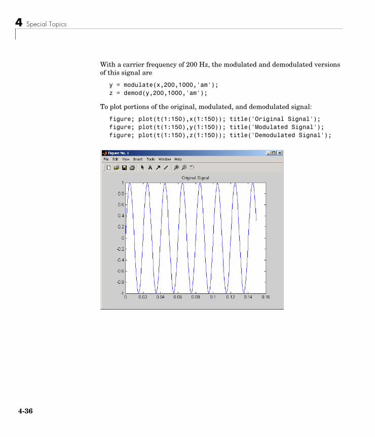
4 Special Topics
4-3
With a carrier frequency of 200 Hz, the modulated and demodulated versions of this signal are
y = modulate(x,200,1000,'am');z = demod(y,200,1000,'am');
To plot portions of the original, modulated, and demodulated signal:
figure; plot(t(1:150),x(1:150)); title('Original Signal');figure; plot(t(1:150),y(1:150)); title('Modulated Signal');figure; plot(t(1:150),z(1:150)); title('Demodulated Signal');
6
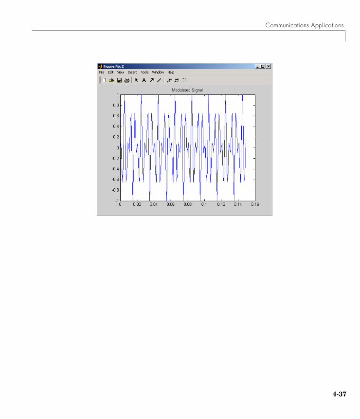
Communications Applications
4-37
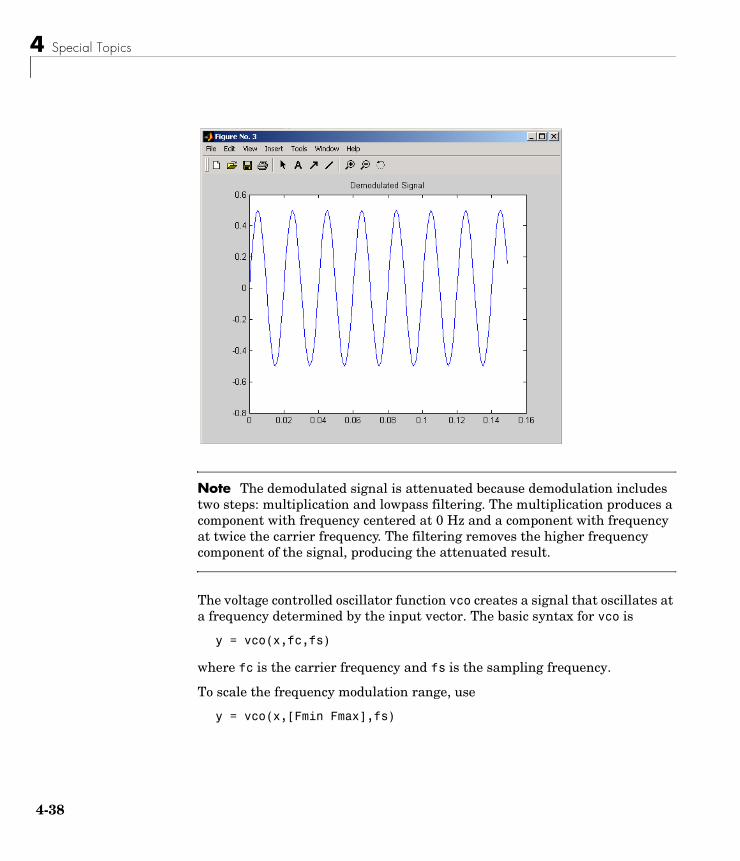
4 Special Topics
4-3
Note The demodulated signal is attenuated because demodulation includes two steps: multiplication and lowpass filtering. The multiplication produces a component with frequency centered at 0 Hz and a component with frequency at twice the carrier frequency. The filtering removes the higher frequency component of the signal, producing the attenuated result.
The voltage controlled oscillator function vco creates a signal that oscillates at a frequency determined by the input vector. The basic syntax for vco is
y = vco(x,fc,fs)
where fc is the carrier frequency and fs is the sampling frequency.
To scale the frequency modulation range, use
y = vco(x,[Fmin Fmax],fs)
8

Communications Applications
In this case, vco scales the frequency modulation range so values of x on the interval [-1 1] map to oscillations of frequency on [Fmin Fmax].
If the input x is an array, vco produces an array whose columns oscillate according to the columns of x.
See “FFT-Based Time-Frequency Analysis” on page 4-34 for an example using the vco function.
4-39
4 Special Topics
4-4
DeconvolutionDeconvolution, or polynomial division, is the inverse operation of convolution. Deconvolution is useful in recovering the input to a known filter, given the filtered output. This method is very sensitive to noise in the coefficients, however, so use caution in applying it.
The syntax for deconv is
[q,r] = deconv(b,a)
where b is the polynomial dividend, a is the divisor, q is the quotient, and r is the remainder.
To try deconv, first convolve two simple vectors a and b (see Chapter 1, “Signal Processing Basics” for a description of the convolution function):
a = [1 2 3];b = [4 5 6];c = conv(a,b)
c = 4 13 28 27 18
Now use deconv to deconvolve b from c:
[q,r] = deconv(c,a)
q = 4 5 6
r = 0 0 0 0 0
0
Specialized Transforms
Specialized TransformsIn addition to the discrete Fourier transform (see fft), the Signal Processing Toolbox and the MATLAB environment together provide the following transform functions:
• The chirp z-transform (CZT), useful in evaluating the z-transform along contours other than the unit circle. The chirp z-transform is also more efficient than the DFT algorithm for the computation of prime-length transforms, and it is useful in computing a subset of the DFT for a sequence.
• The discrete cosine transform (DCT), closely related to the DFT. The DCT’s energy compaction properties are useful for applications like signal coding.
• The Hilbert transform, which facilitates the formation of the analytic signal. The analytic signal is useful in the area of communications, particularly in bandpass signal processing.
Chirp z-TransformThe chirp z-transform, or CZT, computes the z-transform along spiral contours in the z-plane for an input sequence. Unlike the DFT, the CZT is not constrained to operate along the unit circle, but can evaluate the z-transform along contours described by
where A is the complex starting point, W is a complex scalar describing the complex ratio between points on the contour, and M is the length of the transform.
One possible spiral is
A = 0.8*exp(j*pi/6);W = 0.995*exp(-j*pi*.05);M = 91;z = A*(W.^(-(0:M-1)));zplane([],z.')
zl AW l– l 0 … M 1–, ,=,=
4-41
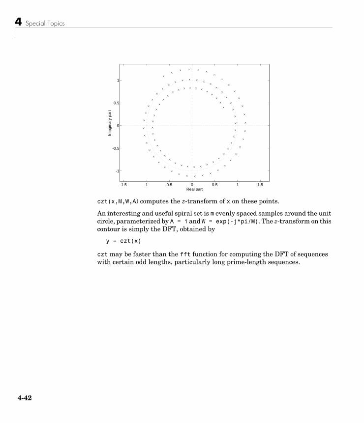
4 Special Topics
4-4
czt(x,M,W,A) computes the z-transform of x on these points.
An interesting and useful spiral set is m evenly spaced samples around the unit circle, parameterized by A = 1 and W = exp(-j*pi/M). The z-transform on this contour is simply the DFT, obtained by
y = czt(x)
czt may be faster than the fft function for computing the DFT of sequences with certain odd lengths, particularly long prime-length sequences.
-1.5 -1 -0.5 0 0.5 1 1.5
-1
-0.5
0
0.5
1
Real part
Imag
inar
y pa
rt
2
Specialized Transforms
Discrete Cosine TransformThe toolbox function dct computes the unitary discrete cosine transform, or DCT, for an input vector or matrix. Mathematically, the unitary DCT of an input sequence x is
where
The DCT is closely related to the discrete Fourier transform; the DFT is actually one step in the computation of the DCT for a sequence. The DCT, however, has better energy compaction properties, with just a few of the transform coefficients representing the majority of the energy in the sequence. The energy compaction properties of the DCT make it useful in applications such as data communications.
The function idct computes the inverse DCT for an input sequence, reconstructing a signal from a complete or partial set of DCT coefficients. The inverse discrete cosine transform is
where
y k( ) w k( ) x n( )π 2n 1–( ) k 1–( )
2N-------------------------------------------cos
n 1=
N
∑ k 1 … N, ,=,=
w k( )
1N
--------- k 1=,
2N---- 2 k N≤ ≤,
=
x n( ) w n( ) y k( )π 2n 1–( ) k 1–( )
2N-------------------------------------------cos
k 1=
N
∑ n 1 … N, ,=,=
w n( )
1N
--------- n 1=,
2N---- 2 n N≤ ≤,
=
4-43
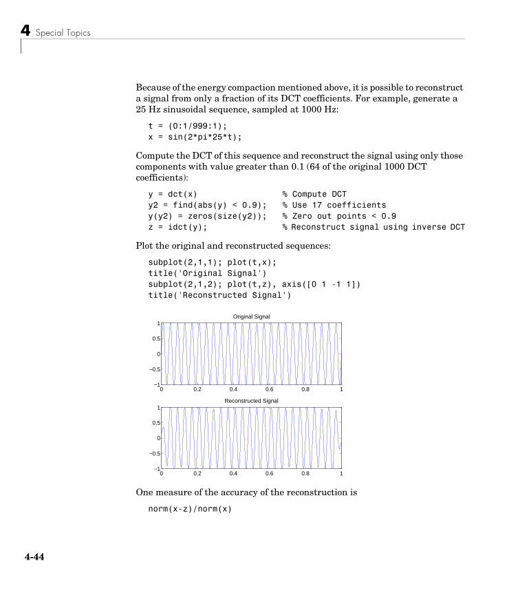
4 Special Topics
4-4
Because of the energy compaction mentioned above, it is possible to reconstruct a signal from only a fraction of its DCT coefficients. For example, generate a 25 Hz sinusoidal sequence, sampled at 1000 Hz:
t = (0:1/999:1);x = sin(2*pi*25*t);
Compute the DCT of this sequence and reconstruct the signal using only those components with value greater than 0.1 (64 of the original 1000 DCT coefficients):
y = dct(x) % Compute DCTy2 = find(abs(y) < 0.9); % Use 17 coefficientsy(y2) = zeros(size(y2)); % Zero out points < 0.9z = idct(y); % Reconstruct signal using inverse DCT
Plot the original and reconstructed sequences:
subplot(2,1,1); plot(t,x);title('Original Signal')subplot(2,1,2); plot(t,z), axis([0 1 -1 1])title('Reconstructed Signal')
One measure of the accuracy of the reconstruction is
norm(x-z)/norm(x)
0 0.2 0.4 0.6 0.8 1−1
−0.5
0
0.5
1Original Signal
0 0.2 0.4 0.6 0.8 1−1
−0.5
0
0.5
1Reconstructed Signal
4
Specialized Transforms
that is, the norm of the difference between the original and reconstructed signals, divided by the norm of the original signal. In this case, the relative error of reconstruction is 0.1443. The reconstructed signal retains approximately 85% of the energy in the original signal.
Hilbert TransformThe toolbox function hilbert computes the Hilbert transform for a real input sequence x and returns a complex result of the same length
y = hilbert(x)
where the real part of y is the original real data and the imaginary part is the actual Hilbert transform. y is sometimes called the analytic signal, in reference to the continuous-time analytic signal. A key property of the discrete-time analytic signal is that its z-transform is 0 on the lower half of the unit circle. Many applications of the analytic signal are related to this property; for example, the analytic signal is useful in avoiding aliasing effects for bandpass sampling operations. The magnitude of the analytic signal is the complex envelope of the original signal.
The Hilbert transform is related to the actual data by a 90° phase shift; sines become cosines and vice versa. To plot a portion of data (solid line) and its Hilbert transform (dotted line):
t = (0:1/1023:1);x = sin(2*pi*60*t);y = hilbert(x);plot(t(1:50),real(y(1:50))), hold onplot(t(1:50),imag(y(1:50)),':'), hold off
4-45
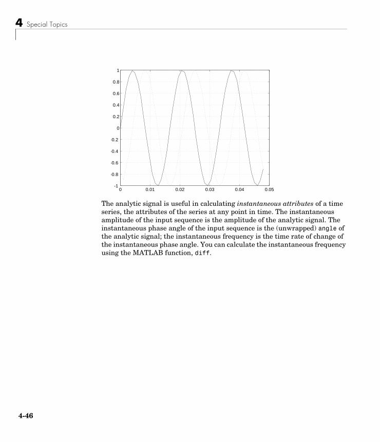
4 Special Topics
4-4
The analytic signal is useful in calculating instantaneous attributes of a time series, the attributes of the series at any point in time. The instantaneous amplitude of the input sequence is the amplitude of the analytic signal. The instantaneous phase angle of the input sequence is the (unwrapped) angle of the analytic signal; the instantaneous frequency is the time rate of change of the instantaneous phase angle. You can calculate the instantaneous frequency using the MATLAB function, diff.
0 0.01 0.02 0.03 0.04 0.05-1
-0.8
-0.6
-0.4
-0.2
0
0.2
0.4
0.6
0.8
1
6

Selected Bibliography
Selected Bibliography[1] Kay, S.M. Modern Spectral Estimation. Englewood Cliffs, NJ: Prentice Hall, 1988.
[2] Oppenheim, A.V., and R.W. Schafer. Discrete-Time Signal Processing. Englewood Cliffs, NJ: Prentice Hall, 1989.
[3] Parks, T.W., and C.S. Burrus. Digital Filter Design. New York: John Wiley & Sons, 1987.
[4] Pratt,W.K. Digital Image Processing. New York: John Wiley & Sons, 1991.
4-47

4 Special Topics
4-4
8
5
FDATool: A Filter Design and Analysis GUIThe following chapter describes the Filter Design and Analysis Tool (FDATool) and provides a detailed example showing how to use this Graphical User Interface.
Overview (p. 5-2) Introduction to the tool
Opening FDATool (p. 5-7) How to start the tool
Choosing a Response Type (p. 5-9) Setting the filter response type
Choosing a Filter Design Method (p. 5-10) Selecting a design method
Setting the Filter Design Specifications (p. 5-11) Setting the filter parameters
Computing the Filter Coefficients (p. 5-15) Calculating the filter
Analyzing the Filter (p. 5-16) Tools for analyzing the filter
Editing the Filter Using the Pole/Zero Editor (p. 5-21)
Changing the filter by changing poles or zeros
Converting the Filter Structure (p. 5-25) Changing the filter structure
Importing a Filter Design (p. 5-28) Bringing a filter design into the tool
Exporting a Filter Design (p. 5-32) Sending the filter design outside the tool
Generating a C Header File (p. 5-36) Create C code of the filter design
Generating an M-File (p. 5-39) Creating MATLAB code of the filter design
Managing Filters in the Current Session (p. 5-40) Working with multiple filters
Saving and Opening Filter Design Sessions (p. 5-42)
Working with tool sessions
5 FDATool: A Filter Design and Analysis GUI
5-2
Overview
Note The Filter Design and Analysis Tool (FDATool) requires resolution of at least 800 by 600.
The Filter Design and Analysis Tool (FDATool) is a powerful user interface for designing and analyzing filters. FDATool enables you to quickly design digital FIR or IIR filters by setting filter performance specifications, by importing filters from your MATLAB workspace, by directly specifying filter coefficients, or by adding, moving or deleting poles and zeros. FDATool also provides tools for analyzing filters, such as magnitude and phase response plots and pole-zero plots. FVTool, which can be launched from FDATool, provides a separate window for analyzing filters. You can use FDATool as a convenient alternative to the command line filter design functions.
Below is a brief introduction to the FDATool that will give you a better understanding of how it can be used.
Note If you have installed external hardware or targets that interact with FDATool, you may see additional options in FDATool. Refer to the specific hardware or target manual for information on these options. These toolboxes/targets are integrated with FDATool:
Filter Design Toolbox
Embedded Target for Texas Instruments C6000 DSP
Link for Code Composer Studio
Signal Processing Blockset
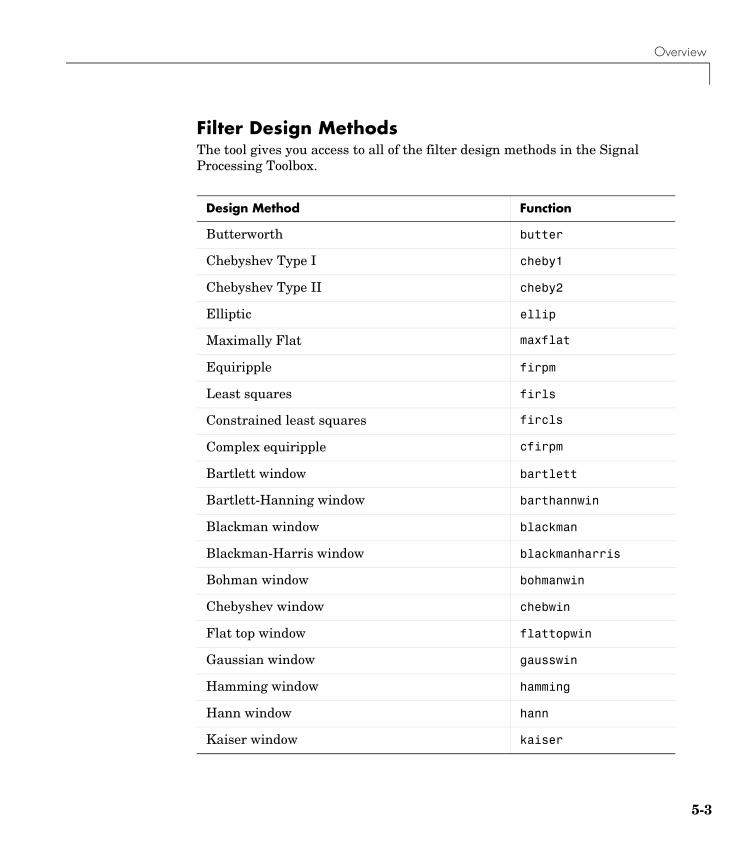
Overview
Filter Design MethodsThe tool gives you access to all of the filter design methods in the Signal Processing Toolbox.
Design Method Function
Butterworth butter
Chebyshev Type I cheby1
Chebyshev Type II cheby2
Elliptic ellip
Maximally Flat maxflat
Equiripple firpm
Least squares firls
Constrained least squares fircls
Complex equiripple cfirpm
Bartlett window bartlett
Bartlett-Hanning window barthannwin
Blackman window blackman
Blackman-Harris window blackmanharris
Bohman window bohmanwin
Chebyshev window chebwin
Flat top window flattopwin
Gaussian window gausswin
Hamming window hamming
Hann window hann
Kaiser window kaiser
5-3
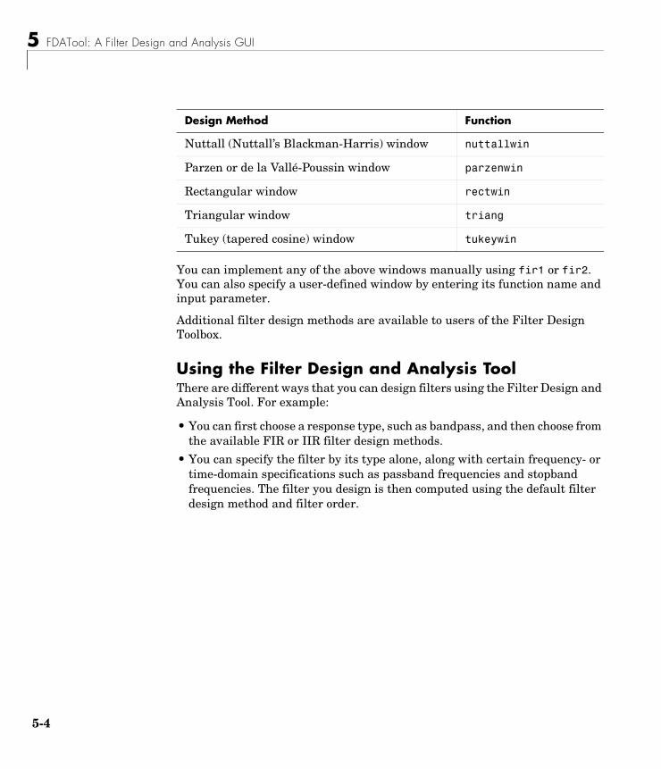
5 FDATool: A Filter Design and Analysis GUI
5-4
You can implement any of the above windows manually using fir1 or fir2. You can also specify a user-defined window by entering its function name and input parameter.
Additional filter design methods are available to users of the Filter Design Toolbox.
Using the Filter Design and Analysis ToolThere are different ways that you can design filters using the Filter Design and Analysis Tool. For example:
• You can first choose a response type, such as bandpass, and then choose from the available FIR or IIR filter design methods.
• You can specify the filter by its type alone, along with certain frequency- or time-domain specifications such as passband frequencies and stopband frequencies. The filter you design is then computed using the default filter design method and filter order.
Nuttall (Nuttall’s Blackman-Harris) window nuttallwin
Parzen or de la Vallé-Poussin window parzenwin
Rectangular window rectwin
Triangular window triang
Tukey (tapered cosine) window tukeywin
Design Method Function
Overview
Analyzing Filter ResponsesOnce you have designed your filter, you can analyze different filter responses in FDATool or in a separate Filter Visualization Tool (fvtool). See “Analyzing the Filter” on page 5-16 for more information:
• Magnitude response (freqz)
• Phase response (phasez)
• Group delay (grpdelay)
• Phase delay (phasedelay)
• Impulse response (impz)
• Step response (stepz)
• Pole-zero plots (zplane)
• Zero-phase response (zerophase)
You can also display the filter coefficients and detailed filter information, export the coefficients to the MATLAB workspace, and create a C header file containing the coefficients.
Filter Design and Analysis Tool PanelsThe Filter Design and Analysis Tool has sidebar buttons that display particular panels in the lower half of the tool. The panels are
• Design Filter. See “Choosing a Filter Design Method” on page 5-10 for more information. You use this panel to
- Design filters from scratch.
- Modify existing filters designed in FDATool.
- Analyze filters.
• Import filter. See “Importing a Filter Design” on page 5-28 for more information. You use this panel to
- Import previously saved filters or filter coefficients that you have stored in the MATLAB workspace.
- Analyze imported filters.
• Pole/Zero Editor. See “Editing the Filter Using the Pole/Zero Editor” on page 5-21. You use this panel to add, delete, and move poles and zeros in your filter design.
5-5
5 FDATool: A Filter Design and Analysis GUI
5-6
If you also have the Filter Design Toolbox installed, additional panels are available:
• Set quantization parameters—Use this panel to quantize double-precision filters that you design in FDATool, quantize double-precision filters that you import into FDATool, and analyze quantized filters.
• Transform filter—Use this panel to change a filter from one response type to another.
• Multirate filter design—Use this panel to create a multirate filter from your existing FIR design, create CIC filters, and and linear and hold interpolators.
If you have the Signal Processing Blockset installed, a Realize Model panel is available. Use this panel to create a Simulink block containing the filter structure.
Getting HelpAt any time, you can right-click or click the What’s this? button, , to get information on the different parts of the tool. You can also use the Help menu to see complete Help information.

Opening FDATool
Opening FDAToolTo open the Filter Design and Analysis Tool, type
fdatool
The Filter Design and Analysis Tool opens with the Design Filter panel displayed.
Note If you are viewing this online, click in the figure below to jump to a description of the procedure for that area of the figure.
5-7

5 FDATool: A Filter Design and Analysis GUI
5-8
Choosing a Response TypeYou can choose from several response types:
• Lowpass
• Raised cosine
• Highpass
• Bandpass
• Bandstop
• Differentiator
• Multiband
• Hilbert transformer
• Arbitrary magnitude
Additional response types are available if you have the Filter Design Toolbox installed.
To design a bandpass filter, select the radio button next to Bandpass in the Response Type region of the GUI.
Note Not all filter design methods are available for all response types. Once you choose your response type, this may restrict the filter design methods available to you. Filter design methods that are not available for a selected response type are removed from the Design Method region of the GUI.

Choosing a Filter Design Method
Choosing a Filter Design MethodYou can use the default filter design method for the response type that you’ve selected, or you can select a filter design method from the available FIR and IIR methods listed in the GUI.
To select the Remez algorithm to compute FIR filter coefficients, select the FIR radio button and choose Equiripple from the list of methods.
5-9
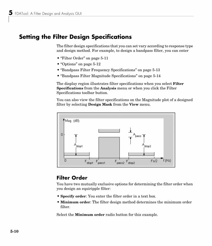
5 FDATool: A Filter Design and Analysis GUI
5-1
Setting the Filter Design SpecificationsThe filter design specifications that you can set vary according to response type and design method. For example, to design a bandpass filter, you can enter
• “Filter Order” on page 5-11
• “Options” on page 5-12
• “Bandpass Filter Frequency Specifications” on page 5-13
• “Bandpass Filter Magnitude Specifications” on page 5-14
The display region illustrates filter specifications when you select Filter Specifications from the Analysis menu or when you click the Filter Specifications toolbar button.
You can also view the filter specifications on the Magnitude plot of a designed filter by selecting Design Mask from the View menu.
Filter OrderYou have two mutually exclusive options for determining the filter order when you design an equiripple filter:
• Specify order: You enter the filter order in a text box.
• Minimum order: The filter design method determines the minimum order filter.
Select the Minimum order radio button for this example.
0
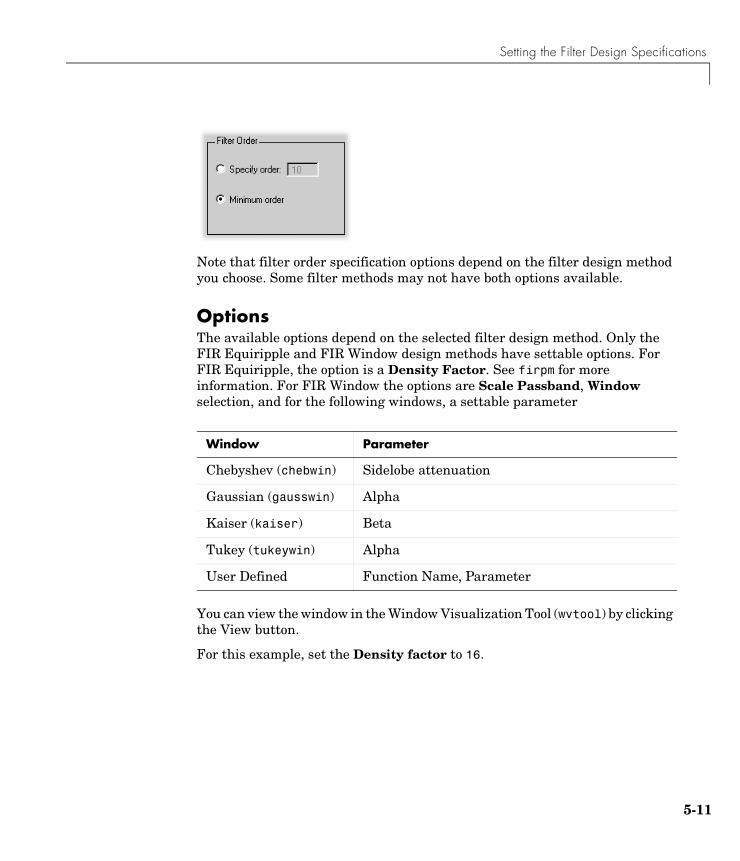
Setting the Filter Design Specifications
Note that filter order specification options depend on the filter design method you choose. Some filter methods may not have both options available.
OptionsThe available options depend on the selected filter design method. Only the FIR Equiripple and FIR Window design methods have settable options. For FIR Equiripple, the option is a Density Factor. See firpm for more information. For FIR Window the options are Scale Passband, Window selection, and for the following windows, a settable parameter
You can view the window in the Window Visualization Tool (wvtool) by clicking the View button.
For this example, set the Density factor to 16.
Window Parameter
Chebyshev (chebwin) Sidelobe attenuation
Gaussian (gausswin) Alpha
Kaiser (kaiser) Beta
Tukey (tukeywin) Alpha
User Defined Function Name, Parameter
5-11
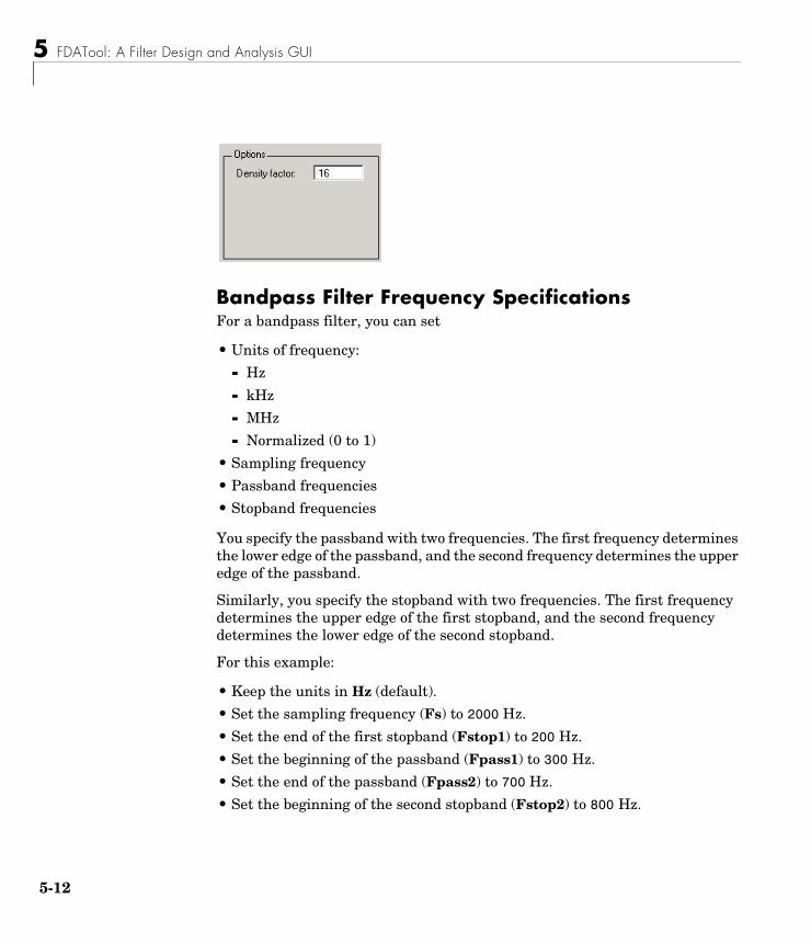
5 FDATool: A Filter Design and Analysis GUI
5-1
Bandpass Filter Frequency SpecificationsFor a bandpass filter, you can set
• Units of frequency:
- Hz
- kHz
- MHz
- Normalized (0 to 1)
• Sampling frequency
• Passband frequencies
• Stopband frequencies
You specify the passband with two frequencies. The first frequency determines the lower edge of the passband, and the second frequency determines the upper edge of the passband.
Similarly, you specify the stopband with two frequencies. The first frequency determines the upper edge of the first stopband, and the second frequency determines the lower edge of the second stopband.
For this example:
• Keep the units in Hz (default).
• Set the sampling frequency (Fs) to 2000 Hz.
• Set the end of the first stopband (Fstop1) to 200 Hz.
• Set the beginning of the passband (Fpass1) to 300 Hz.
• Set the end of the passband (Fpass2) to 700 Hz.
• Set the beginning of the second stopband (Fstop2) to 800 Hz.
2
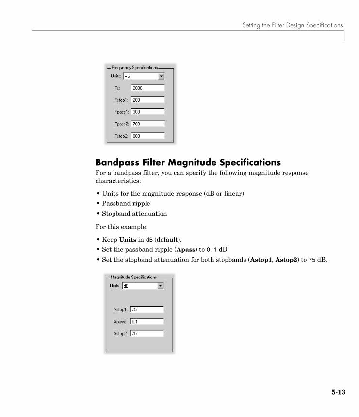
Setting the Filter Design Specifications
Bandpass Filter Magnitude SpecificationsFor a bandpass filter, you can specify the following magnitude response characteristics:
• Units for the magnitude response (dB or linear)
• Passband ripple
• Stopband attenuation
For this example:
• Keep Units in dB (default).
• Set the passband ripple (Apass) to 0.1 dB.
• Set the stopband attenuation for both stopbands (Astop1, Astop2) to 75 dB.
5-13
5 FDATool: A Filter Design and Analysis GUI
5-1
Computing the Filter CoefficientsNow that you’ve specified the filter design, click the Design Filter button to compute the filter coefficients.
Notice that the Design Filter button is disabled once you’ve computed the coefficients for your filter design. This button is enabled again once you make any changes to the filter specifications.
Note You can undo actions, one at a time, by selecting Undo from the Edit menu or by clicking the Undo toolbar button. To redo previously undone actions, select Redo from the Edit menu or click the Redo toolbar button.
4
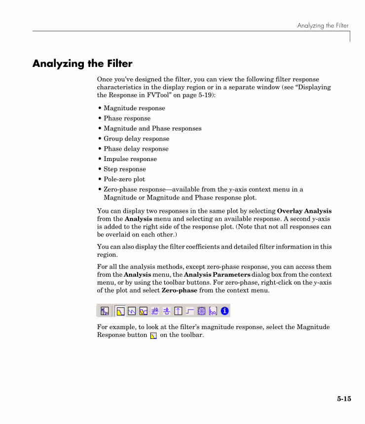
Analyzing the Filter
Analyzing the FilterOnce you’ve designed the filter, you can view the following filter response characteristics in the display region or in a separate window (see “Displaying the Response in FVTool” on page 5-19):
• Magnitude response
• Phase response
• Magnitude and Phase responses
• Group delay response
• Phase delay response
• Impulse response
• Step response
• Pole-zero plot
• Zero-phase response—available from the y-axis context menu in a Magnitude or Magnitude and Phase response plot.
You can display two responses in the same plot by selecting Overlay Analysis from the Analysis menu and selecting an available response. A second y-axis is added to the right side of the response plot. (Note that not all responses can be overlaid on each other.)
You can also display the filter coefficients and detailed filter information in this region.
For all the analysis methods, except zero-phase response, you can access them from the Analysis menu, the Analysis Parameters dialog box from the context menu, or by using the toolbar buttons. For zero-phase, right-click on the y-axis of the plot and select Zero-phase from the context menu.
For example, to look at the filter’s magnitude response, select the Magnitude Response button on the toolbar.
5-15
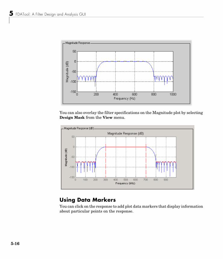
5 FDATool: A Filter Design and Analysis GUI
5-1
You can also overlay the filter specifications on the Magnitude plot by selecting Design Mask from the View menu.
Using Data MarkersYou can click on the response to add plot data markers that display information about particular points on the response.
6
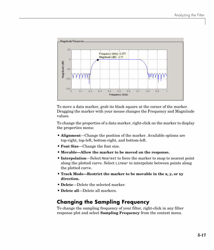
Analyzing the Filter
To move a data marker, grab its black square at the corner of the marker. Dragging the marker with your mouse changes the Frequency and Magnitude values.
To change the properties of a data marker, right-click on the marker to display the properties menu:
• Alignment—Change the position of the marker. Available options are top-right, top-left, bottom-right, and bottom-left.
• Font Size—Change the font size.
• Movable—Allow the marker to be moved on the response.
• Interpolation—Select Nearest to force the marker to snap to nearest point along the plotted curve. Select Linear to interpolate between points along the plotted curve.
• Track Mode—Restrict the marker to be movable in the x, y, or xy direction.
• Delete—Delete the selected marker.
• Delete all—Delete all markers.
Changing the Sampling FrequencyTo change the sampling frequency of your filter, right-click in any filter response plot and select Sampling Frequency from the context menu.
5-17
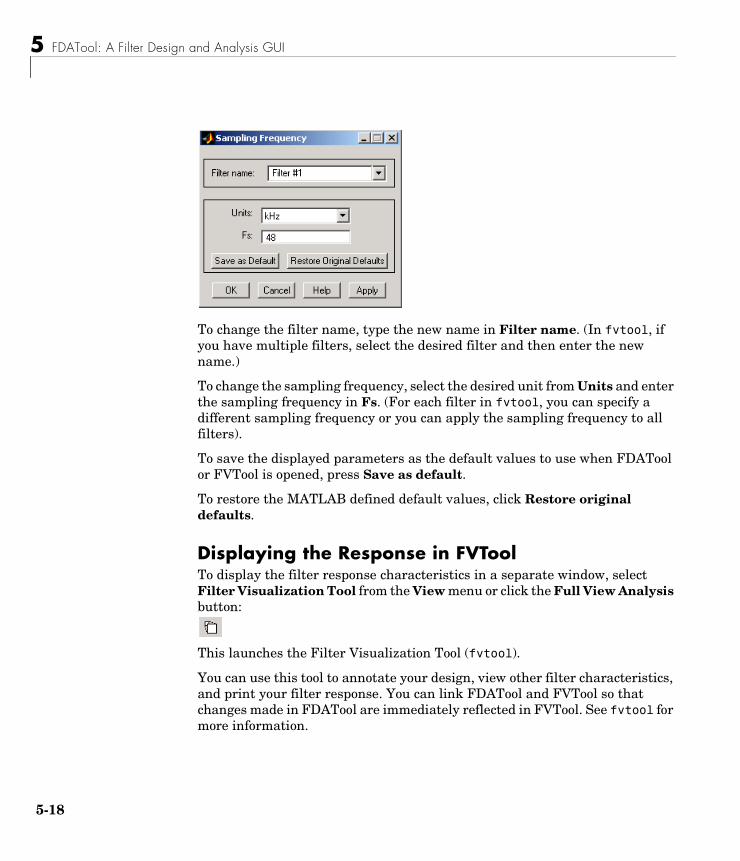
5 FDATool: A Filter Design and Analysis GUI
5-1
To change the filter name, type the new name in Filter name. (In fvtool, if you have multiple filters, select the desired filter and then enter the new name.)
To change the sampling frequency, select the desired unit from Units and enter the sampling frequency in Fs. (For each filter in fvtool, you can specify a different sampling frequency or you can apply the sampling frequency to all filters).
To save the displayed parameters as the default values to use when FDATool or FVTool is opened, press Save as default.
To restore the MATLAB defined default values, click Restore original defaults.
Displaying the Response in FVToolTo display the filter response characteristics in a separate window, select Filter Visualization Tool from the View menu or click the Full View Analysis button:
This launches the Filter Visualization Tool (fvtool).
You can use this tool to annotate your design, view other filter characteristics, and print your filter response. You can link FDATool and FVTool so that changes made in FDATool are immediately reflected in FVTool. See fvtool for more information.
8
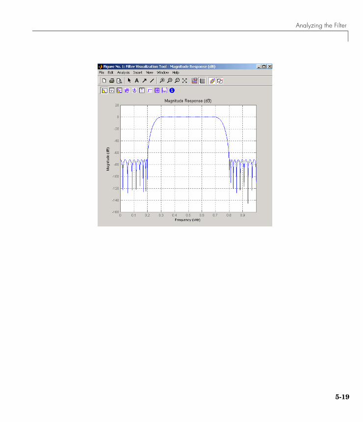
Analyzing the Filter
5-19
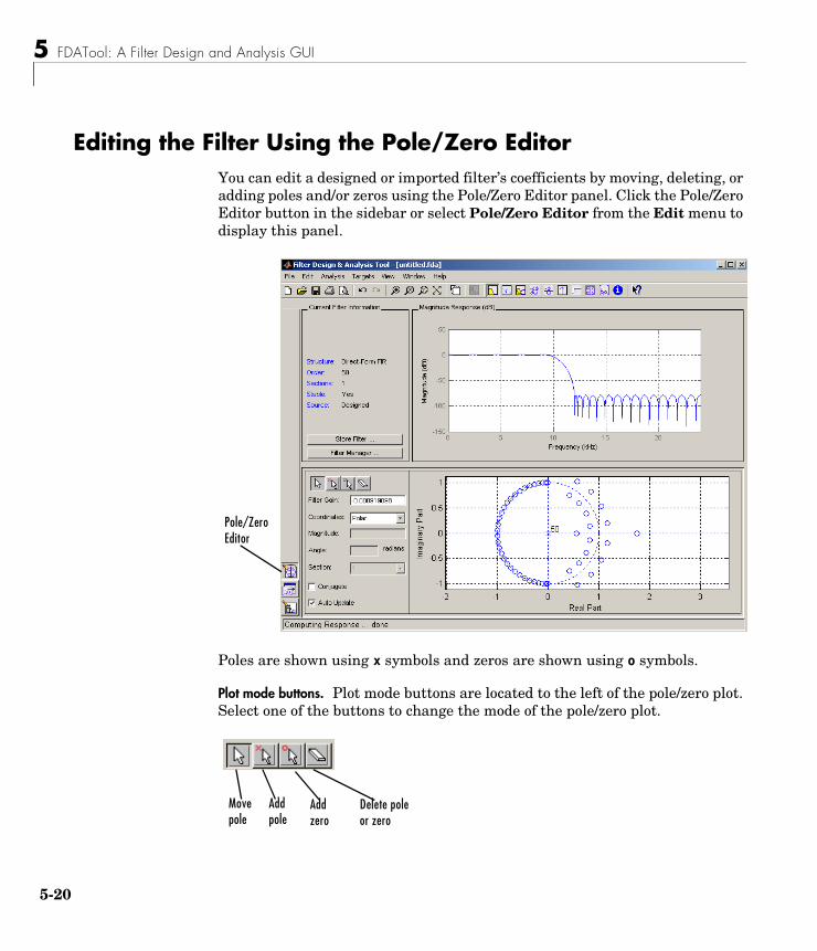
5 FDATool: A Filter Design and Analysis GUI
5-2
Editing the Filter Using the Pole/Zero EditorYou can edit a designed or imported filter’s coefficients by moving, deleting, or adding poles and/or zeros using the Pole/Zero Editor panel. Click the Pole/Zero Editor button in the sidebar or select Pole/Zero Editor from the Edit menu to display this panel.
Poles are shown using x symbols and zeros are shown using o symbols.
Plot mode buttons. Plot mode buttons are located to the left of the pole/zero plot. Select one of the buttons to change the mode of the pole/zero plot.
Pole/Zero Editor
Move pole
Delete pole or zero
Add zero
Add pole
0
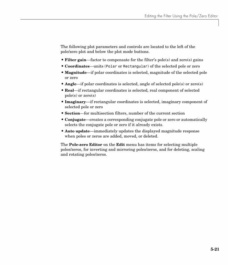
Editing the Filter Using the Pole/Zero Editor
The following plot parameters and controls are located to the left of the pole/zero plot and below the plot mode buttons.
• Filter gain—factor to compensate for the filter’s pole(s) and zero(s) gains
• Coordinates—units (Polar or Rectangular) of the selected pole or zero
• Magnitude—if polar coordinates is selected, magnitude of the selected pole or zero
• Angle—if polar coordinates is selected, angle of selected pole(s) or zero(s)
• Real—if rectangular coordinates is selected, real component of selected pole(s) or zero(s)
• Imaginary—if rectangular coordinates is selected, imaginary component of selected pole or zero
• Section—for multisection filters, number of the current section
• Conjugate—creates a corresponding conjugate pole or zero or automatically selects the conjugate pole or zero if it already exists.
• Auto update—immediately updates the displayed magnitude response when poles or zeros are added, moved, or deleted.
The Pole-zero Editor on the Edit menu has items for selecting multiple poles/zeros, for inverting and mirroring poles/zeros, and for deleting, scaling and rotating poles/zeros.
5-21
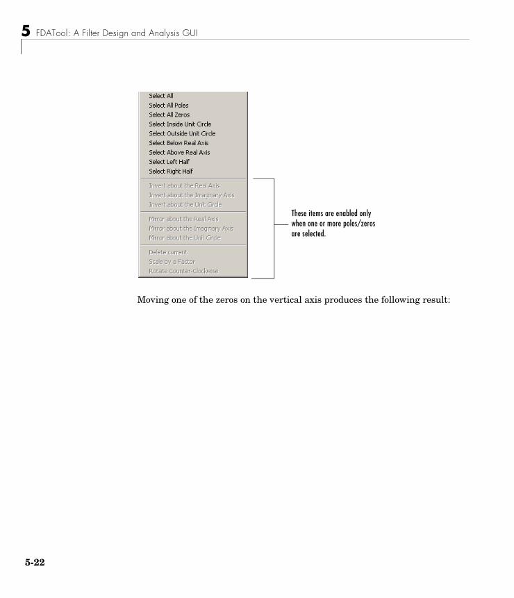
5 FDATool: A Filter Design and Analysis GUI
5-2
Moving one of the zeros on the vertical axis produces the following result:
These items are enabled only when one or more poles/zeros are selected.
2
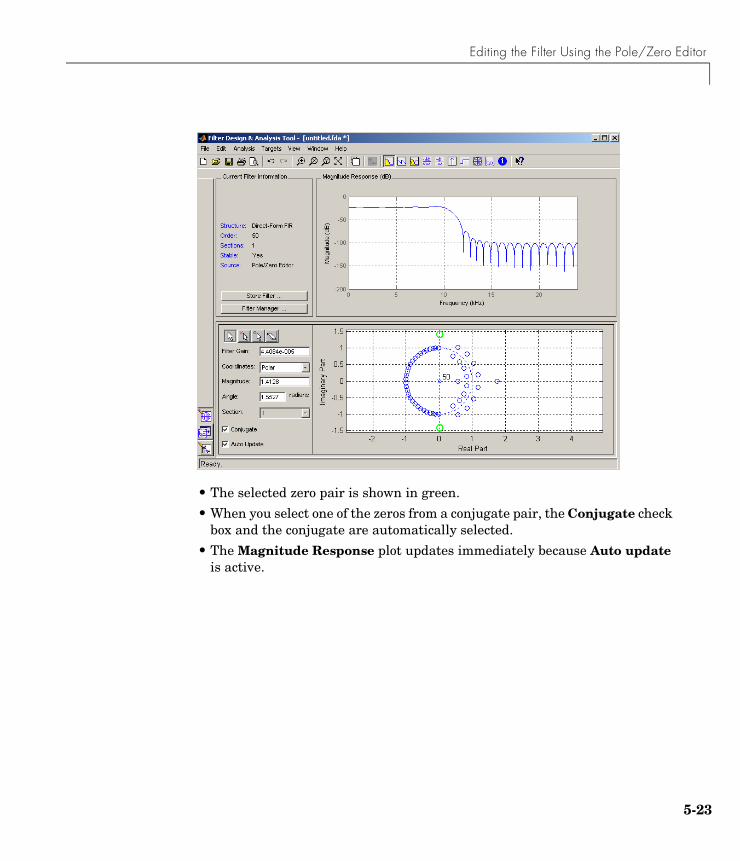
Editing the Filter Using the Pole/Zero Editor
• The selected zero pair is shown in green.
• When you select one of the zeros from a conjugate pair, the Conjugate check box and the conjugate are automatically selected.
• The Magnitude Response plot updates immediately because Auto update is active.
5-23
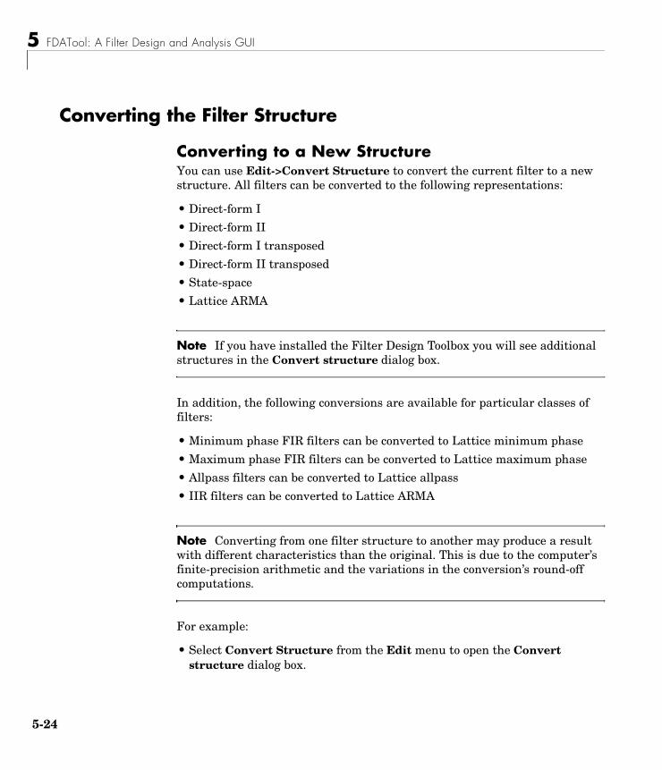
5 FDATool: A Filter Design and Analysis GUI
5-2
Converting the Filter Structure
Converting to a New StructureYou can use Edit->Convert Structure to convert the current filter to a new structure. All filters can be converted to the following representations:
• Direct-form I
• Direct-form II
• Direct-form I transposed
• Direct-form II transposed
• State-space
• Lattice ARMA
Note If you have installed the Filter Design Toolbox you will see additional structures in the Convert structure dialog box.
In addition, the following conversions are available for particular classes of filters:
• Minimum phase FIR filters can be converted to Lattice minimum phase
• Maximum phase FIR filters can be converted to Lattice maximum phase
• Allpass filters can be converted to Lattice allpass
• IIR filters can be converted to Lattice ARMA
Note Converting from one filter structure to another may produce a result with different characteristics than the original. This is due to the computer’s finite-precision arithmetic and the variations in the conversion’s round-off computations.
For example:
• Select Convert Structure from the Edit menu to open the Convert structure dialog box.
4
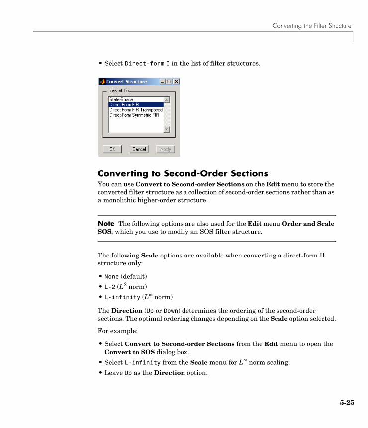
Converting the Filter Structure
• Select Direct-form I in the list of filter structures.
Converting to Second-Order SectionsYou can use Convert to Second-order Sections on the Edit menu to store the converted filter structure as a collection of second-order sections rather than as a monolithic higher-order structure.
Note The following options are also used for the Edit menu Order and Scale SOS, which you use to modify an SOS filter structure.
The following Scale options are available when converting a direct-form II structure only:
• None (default)
• L-2 (L2 norm)
• L-infinity (L∞ norm)
The Direction (Up or Down) determines the ordering of the second-order sections. The optimal ordering changes depending on the Scale option selected.
For example:
• Select Convert to Second-order Sections from the Edit menu to open the Convert to SOS dialog box.
• Select L-infinity from the Scale menu for L∞ norm scaling.
• Leave Up as the Direction option.
5-25

5 FDATool: A Filter Design and Analysis GUI
5-2
Note To convert from second-order sections back to a single section, use Convert to Single Section on the Edit menu.
6
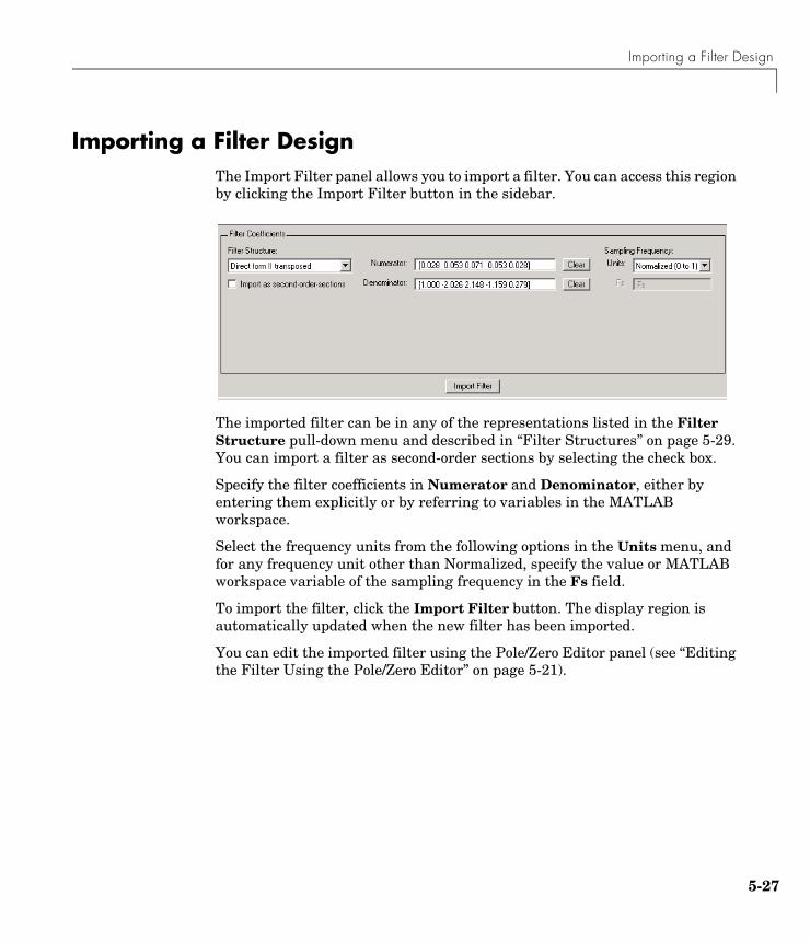
Importing a Filter Design
Importing a Filter DesignThe Import Filter panel allows you to import a filter. You can access this region by clicking the Import Filter button in the sidebar.
The imported filter can be in any of the representations listed in the Filter Structure pull-down menu and described in “Filter Structures” on page 5-29. You can import a filter as second-order sections by selecting the check box.
Specify the filter coefficients in Numerator and Denominator, either by entering them explicitly or by referring to variables in the MATLAB workspace.
Select the frequency units from the following options in the Units menu, and for any frequency unit other than Normalized, specify the value or MATLAB workspace variable of the sampling frequency in the Fs field.
To import the filter, click the Import Filter button. The display region is automatically updated when the new filter has been imported.
You can edit the imported filter using the Pole/Zero Editor panel (see “Editing the Filter Using the Pole/Zero Editor” on page 5-21).
5-27
5 FDATool: A Filter Design and Analysis GUI
5-2
Filter StructuresThe available filter structures are:
• Direct-form, which includes direct-form I, direct-form II, direct-form I transposed, direct-form II transposed, and direc-form FIR
• Lattice, which includes lattice allpass, lattice MA min phase, lattice MA max phase, and lattice ARMA
• State-space
• Discrete-time filter (dfilt object)
The structure that you choose determines the type of coefficients that you need to specify in the text fields to the right.
Direct-formFor direct-form I, direct-form II, direct-form I transposed, and direct-form II transposed, specify the filter by its transfer function representation
• The Numerator field specifies a variable name or value for the numerator coefficient vector b, which contains m+1 coefficients in descending powers of z.
• The Denominator field specifies a variable name or value for the denominator coefficient vector a, which contains n+1 coefficients in descending powers of z. For FIR filters, the Denominator is 1.
Filters in transfer function form can be produced by all of the Signal Processing Toolbox filter design functions (such as fir1, fir2, firpm, butter, yulewalk). See “Transfer Function” on page 1-34 for more information.
Importing as second-order sections . For all direct-form structures, except Direct-form FIR, you an import the filter in its second-order section representation:
The Gain field specifies a variable name or a value for the gain g, and the SOS Matrix field specifies a variable name or a value for the L-by-6 SOS matrix
H z( )B z( )A z( )----------- b 1( ) b 2( )z 1– b m 1+( )z m–+ + +
a 1( ) a 2( )z 1– a n 1+( )z n–+ + +---------------------------------------------------------------------------------------= =
H z( ) g Hk z( )
k 1=
L
∏ gb0k b1kz 1– b2kz 2–+ +
1 a1kz 1– a2kz 2–+ +----------------------------------------------------------
k 1=
L
∏= =
8
Importing a Filter Design
whose rows contain the numerator and denominator coefficients bik and aik of the second-order sections of H(z).
Filters in second-order section form can be produced by functions such as tf2sos, zp2sos, ss2sos, and sosfilt. See “Second-Order Sections (SOS)” on page 1-39 for more information.
State-SpaceFor State-Space, specify the filter by its state-space representation:
The A, B, C, and D fields each specify a variable name or a value for the matrices in this system.
Filters in state-space form can be produced by functions such as tf2ss and zp2ss. See “State-Space” on page 1-36 for more information.
LatticeFor lattice allpass, lattice minimum and maximum phase, and lattice ARMA filters, specify the filter by its lattice representation:
• For lattice allpass, the Lattice coeff field specifies the lattice (reflection) coefficients, k(1) to k(N), where N is the filter order.
• For lattice MA (minimum or maximum phase), the Lattice coeff field specifies the lattice (reflection) coefficients, k(1) to k(N), where N is the filter order.
• For lattice ARMA, the Lattice coeff field specifies the lattice (reflection) coefficients, k(1) to k(N), and the Ladder coeff field specifies the ladder coefficients, v(1) to v(N+1), where N is the filter order.
SOS
b01 b11 b21 1 a11 a21
b02 b12 b22 1 a12 a22
b0L b1L b2L 1 a1L a2L
=
x· Ax Bu+=
y Cx Du+=
5-29
5 FDATool: A Filter Design and Analysis GUI
5-3
Filters in lattice form can be produced by tf2latc. See “Lattice Structure” on page 1-39 for more information.
Discrete-time Filter (dfilt object)For Discrete-time filter, specify the name of the dfilt object. See dfilt for more information.
Multirate Filter (mfilt object)For Multirate filter, specify the name of the mfilt object. See mfilt in the Filter Design Toolbox for more information.
0
Exporting a Filter Design
Exporting a Filter DesignYou can save your filter design by
• “Exporting Coefficients or Objects to the Workspace” on page 5-32
• “Exporting Coefficients to an ASCII File” on page 5-34
• “Exporting Coefficients or Objects to a MAT-File” on page 5-34
• “Exporting to SPTool” on page 5-35
You can also send your filter to a C header file or generate an M-file. The M-file contains code that replicates the filter you designed. See the following sections:
• “Generating a C Header File” on page 5-36
• “Generating an M-File” on page 5-39
Exporting Coefficients or Objects to the WorkspaceYou can save the filter either as filter coefficients variables or as a dfilt or mfilt filter object variable. (Note that you must have the Filter Design Toolbox installed to save as an mfilt.) To save the filter to the MATLAB workspace:
1 Select Export from the File menu. The Export dialog box appears.
2 Select Workspace from the Export To menu.
3 Select Coefficients from the Export As menu to save the filter coefficients or select Objects to save the filter in a filter object.
4 For coefficients, assign variable names using the Numerator (for FIR filters) or Numerator and Denominator (for IIR filters), or SOS Matrix and Scale Values (for IIR filters in second-order section form) text boxes in the Variable Names region.
For objects, assign the variable name in the Discrete Filter (or Quantized Filter) text box. If you have variables with the same names in your workspace and you want to overwrite them, select the Overwrite Variables check box.
5 Click the OK button.
5-31
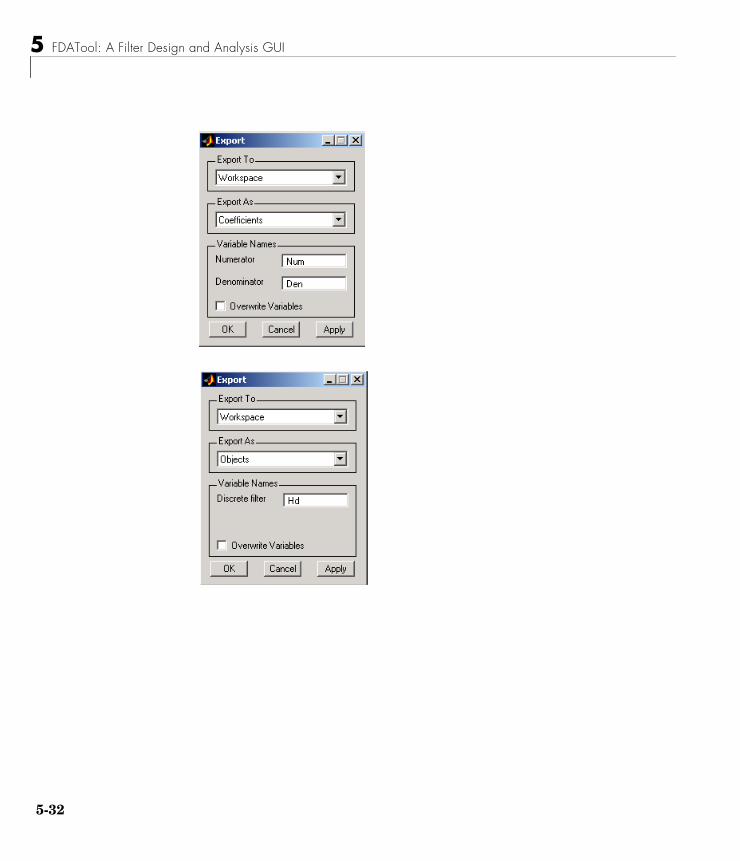
5 FDATool: A Filter Design and Analysis GUI
5-3
2
Exporting a Filter Design
Exporting Coefficients to an ASCII FileTo save filter coefficients to a text file,
1 Select Export from the File menu. The Export dialog box appears.
2 Select Coefficients File (ASCII) from the Export To menu.
3 Click the OK button. The Export Filter Coefficients to .FCF File dialog box appears.
4 Choose or enter a filename and click the Save button.
The coefficients are saved in the text file that you specified, and the MATLAB Editor opens to display the file. The text file also contains comments with the MATLAB version number, the Signal Processing Toolbox version number, and filter information.
Exporting Coefficients or Objects to a MAT-FileTo save filter coefficients or a filter object as variables in a MAT-file:
1 Select Export from the File menu. The Export dialog box appears.
2 Select MAT-file from the Export To menu.
3 Select Coefficients from the Export As menu to save the filter coefficients or select Objects to save the filter in a filter object.
4 For coefficients, assign variable names using the Numerator (for FIR filters) or Numerator and Denominator (for IIR filters), or SOS Matrix and Scale Values (for IIR filters in second-order section form) text boxes in the Variable Names region.
For objects, assign the variable name in the Discrete Fitler (or Quantized Filter) text box. If you have variables with the same names in your workspace and you want to overwrite them, select the Overwrite Variables check box.
5 Click the OK button. The Export to a MAT-File dialog box appears.
6 Choose or enter a filename and click the Save button.
5-33
5 FDATool: A Filter Design and Analysis GUI
5-3
See also “Saving and Opening Filter Design Sessions” on page 5-42.
Exporting to SPToolYou may want to use your designed filter in SPTool to do signal processing and analysis:
1 Select Export from the File menu. The Export dialog box appears.
2 Select SPTool from the Export To menu.
3 Select Coefficients from the Export As menu to save the filter coefficients or select Objects to save the filter in a filter object.
4 Assign the variable name in the Discrete Filter (or Quantized Filter) text box. If you have variables with the same names in your workspace and you want to overwrite them, select the Overwrite Variables check box.
5 Click the OK button.
SPTool opens and the current FDATool filter appears in the Filter area list as the specified variable name followed by (Imported).
Note If you are using the Filter Design Toolbox and export a quantized filter, only the values of its quantized coefficients are exported. The reference coefficients are not exported. SPTool does not restrict the coefficient values, so if you edit them in SPTool by moving poles or zeros, the filter will no longer be in quantized form.
4
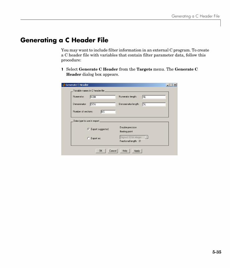
Generating a C Header File
Generating a C Header FileYou may want to include filter information in an external C program. To create a C header file with variables that contain filter parameter data, follow this procedure:
1 Select Generate C Header from the Targets menu. The Generate C Header dialog box appears.
5-35
5 FDATool: A Filter Design and Analysis GUI
5-3
2 Enter the variable names to be used in the C header file. The particular filter structure determines the variables that are created in the file
*length variables contain the total number of coefficients of that type.
Note Variable names cannot be C language reserved words, such as “for.”
3 Select Export Suggested to use the suggested data type or select Export As and select the desired data type from the pull-down.
Note If you do not have the Filter Design Toolbox installed, selecting any data type other than double-precision floating point results in a filter that does not exactly match the one you designed in the FDATool. This is due to rounding and truncating differences.
Filter Structure Variable Parameter
Direct-form IDirect-form IIDirect-form I transposedDirect-form II transposed
Numerator, Numerator length*, Denominator, Denominator length*, and Number of sections (inactive if filter has only one section)
Lattice ARMA Lattice coeffs, Lattice coeffs length*, Ladder coeffs, Ladder coeffs length*, Number of sections (inactive if filter has only one section)
Lattice MA Lattice coeffs, Lattice coeffs length*, and Number of sections (inactive if filter has only one section)
Direct-form FIR Direct-form FIR transposed
Numerator, Numerator length*, and Number of sections (inactive if filter has only one section)
6

Generating a C Header File
4 Click OK to save the file and close the dialog box or click Apply to save the file, but leave the dialog box open for additional C header file definitions.
5-37
5 FDATool: A Filter Design and Analysis GUI
5-3
Generating an M-FileYou can generate an M-file that contains all the code used to create the filter you designed in FDATool. Select Generate M-file from the File menu and specify the filename in the Generate M-file dialog box.
The following is a sample generated M-file of the default FDATool filter.
function Hd = untitled%UNTITLED Returns a discrete-time filter object
%% M-file generated by MATLAB(R) 6.5 and the Signal Processing% Toolbox 6.0.%% Generated on: 24-Oct-2002 09:46:59%
% Remez FIR Lowpass filter designed using the firpm function.
% All frequency values are in Hz.Fs = 48000; % Sampling Frequency
Fpass = 9600; % Passband FrequencyFstop = 12000; % Stopband FrequencyDpass = 0.057501127785; % Passband RippleDstop = 0.0001; % Stopband Attenuationdens = 16; % Density Factor
% Calculate the order from the parameters using firpmord.[N, Fo, Ao, W] = firpmord([Fpass, Fstop]/(Fs/2), [1 0], ...[Dpass, Dstop]);
% Calculate the coefficients using the firpm function.b = firpm(N, Fo, Ao, W, dens);Hd = dfilt.dffir(b);
% [EOF]
8
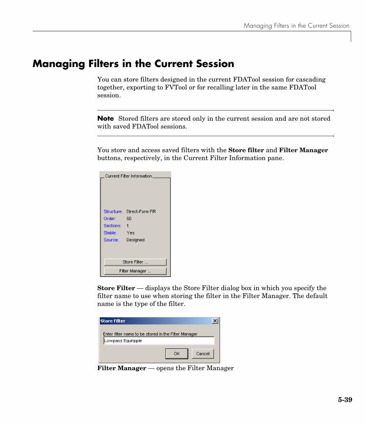
Managing Filters in the Current Session
Managing Filters in the Current SessionYou can store filters designed in the current FDATool session for cascading together, exporting to FVTool or for recalling later in the same FDATool session.
Note Stored filters are stored only in the current session and are not stored with saved FDATool sessions.
You store and access saved filters with the Store filter and Filter Manager buttons, respectively, in the Current Filter Information pane.
Store Filter — displays the Store Filter dialog box in which you specify the filter name to use when storing the filter in the Filter Manager. The default name is the type of the filter.
Filter Manager — opens the Filter Manager
5-39
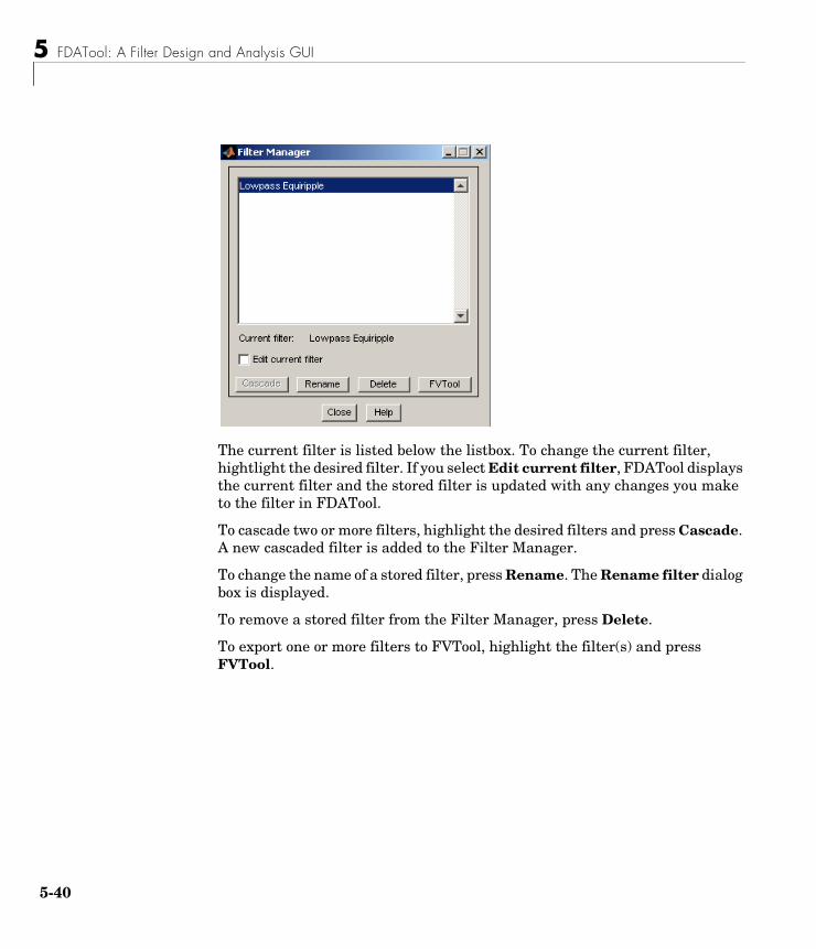
5 FDATool: A Filter Design and Analysis GUI
5-4
The current filter is listed below the listbox. To change the current filter, hightlight the desired filter. If you select Edit current filter, FDATool displays the current filter and the stored filter is updated with any changes you make to the filter in FDATool.
To cascade two or more filters, highlight the desired filters and press Cascade. A new cascaded filter is added to the Filter Manager.
To change the name of a stored filter, press Rename. The Rename filter dialog box is displayed.
To remove a stored filter from the Filter Manager, press Delete.
To export one or more filters to FVTool, highlight the filter(s) and press FVTool.
0
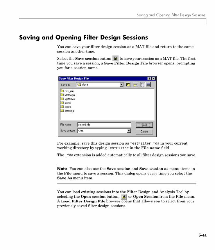
Saving and Opening Filter Design Sessions
Saving and Opening Filter Design SessionsYou can save your filter design session as a MAT-file and return to the same session another time.
Select the Save session button to save your session as a MAT-file. The first time you save a session, a Save Filter Design File browser opens, prompting you for a session name.
For example, save this design session as TestFilter.fda in your current working directory by typing TestFilter in the File name field.
The .fda extension is added automatically to all filter design sessions you save.
Note You can also use the Save session and Save session as menu items in the File menu to save a session. This dialog opens every time you select the Save As menu item.
You can load existing sessions into the Filter Design and Analysis Tool by selecting the Open session button, or Open Session from the File menu. A Load Filter Design File browser opens that allows you to select from your previously saved filter design sessions.
5-41

5 FDATool: A Filter Design and Analysis GUI
5-4
2
6
SPTool: A Signal Processing GUI SuiteThe following chapter describes the Signal Processing Tool (SPTool) and provides a detailed example showing how to use this Graphical User Interface.
SPTool: An Interactive Signal Processing Environment (p. 6-3)
Overview of the tool
Opening SPTool (p. 6-5) How to start the tool
Getting Context-Sensitive Help (p. 6-7) How to get help
Signal Browser (p. 6-8) Viewing signals
Filter Designer (p. 6-11) Designing filters
Filter Visualization Tool (p. 6-14) Viewing and analyzing filters
Spectrum Viewer (p. 6-18) Viewing spectra
Filtering and Analysis of Noise (p. 6-21) Full example using the tool
Exporting Signals, Filters, and Spectra (p. 6-33) Sending data out of the tool
Accessing Filter Parameters (p. 6-35) Using MATLAB to access saved filter parameters
Importing Filters and Spectra into SPTool (p. 6-40)
Bringing data into the tool
Loading Variables from the Disk (p. 6-44) Bringing data from a disk into the tool
Selecting Signals, Filters, and Spectra in SPTool (p. 6-45)
Selecting data
Editing Signals, Filters, or Spectra in SPTool (p. 6-46)
Editing data
Designing a Filter with the Pole/Zero Editor (p. 6-47)
Using the Pole/Zero Editor

6 SPTool: A Signal Processing GUI Suite
6-2
Redesigning a Filter Using the Magnitude Plot (p. 6-50)
Changing the filter design using Magnitude plot
Setting Preferences (p. 6-51) Customizing the tool
Making Signal Measurements with Markers (p. 6-53)
Measuring signals
SPTool: An Interactive Signal Processing Environment
SPTool: An Interactive Signal Processing EnvironmentSPTool is an interactive GUI for digital signal processing that can be used to
• Analyze signals
• Design filters
• Analyze (view) filters
• Filter signals
• Analyze signal spectra
You can accomplish these tasks using four GUIs that you access from within SPTool:
• The Signal Browser is for analyzing signals. You can also play portions of signals using your computer’s audio hardware.
• The Filter Designer is for designing or editing FIR and IIR digital filters. Most of the Signal Processing Toolbox filter design methods available at the command line are also available in the Filter Designer. Additionally, you can design a filter by using the Pole/Zero Editor to graphically place poles and zeros on the z-plane.
• The Filter Visualization Tool is for analyzing filter characteristics. See “Filter Visualization Tool” on page 6-14.
• The Spectrum Viewer is for spectral analysis. You can use the Signal Processing Toolbox spectral estimation methods to estimate the power spectral density of a signal. See “Spectrum Viewer” on page 6-18.
6-3
6 SPTool: A Signal Processing GUI Suite
6-4
SPTool Data StructuresYou can use SPTool to analyze signals, filters, or spectra that you create at the MATLAB command line.
You can bring signals, filters, or spectra from the MATLAB workspace into the SPTool workspace using the Import item under the File menu. Signals, filters, or spectra that you create in (or import into) the SPTool workspace exist as MATLAB structures. See the MATLAB documentation for more information on MATLAB structures.
When you use the Export item under the File menu to save signals, filters, and spectra that you create or modify in SPTool, these are also saved as MATLAB structures.
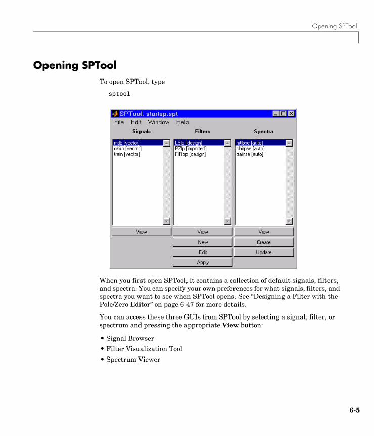
Opening SPTool
Opening SPToolTo open SPTool, type
sptool
When you first open SPTool, it contains a collection of default signals, filters, and spectra. You can specify your own preferences for what signals, filters, and spectra you want to see when SPTool opens. See “Designing a Filter with the Pole/Zero Editor” on page 6-47 for more details.
You can access these three GUIs from SPTool by selecting a signal, filter, or spectrum and pressing the appropriate View button:
• Signal Browser
• Filter Visualization Tool
• Spectrum Viewer
6-5

6 SPTool: A Signal Processing GUI Suite
6-6
You can access the Filter Designer GUI by pressing the New button to create a new filter or the Edit button to edit a selected filter. The Apply button applies a selected filter to a selected signal.
The Create button opens the Spectrum Viewer and creates the power spectral density of the selected signal. The Update button opens the Spectrum Viewer for the selected spectrum.

Getting Context-Sensitive Help
Getting Context-Sensitive HelpTo find information on a particular region of the Signal Browser, Filter Designer, or Spectrum Viewer:
1 Press the What’s this? button, .
2 Click on the region of the GUI you want information on.
You can also use the What’s this? menu item in the Help menu to launch context-sensitive help.
6-7

6 SPTool: A Signal Processing GUI Suite
6-8
Signal BrowserYou can use the Signal Browser to display and analyze signals listed in the Signals list box in SPTool.
Using the Signal Browser you can:
• Analyze and compare vector or array (matrix) signals.
• Zoom in on portions of signal data.
• Measure a variety of characteristics of signal data.
• Compare multiple signals.
• Play portions of signal data on audio hardware.
• Print signal plots.
Opening the Signal BrowserTo open the Signal Browser from SPTool:
1 Select one or more signals in the Signals list in SPTool
2 Press the View button under the Signals list
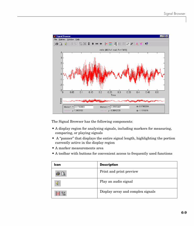
Signal Browser
The Signal Browser has the following components:
• A display region for analyzing signals, including markers for measuring, comparing, or playing signals
• A “panner” that displays the entire signal length, highlighting the portion currently active in the display region
• A marker measurements area
• A toolbar with buttons for convenient access to frequently used functions
Icon Description
Print and print preview
Play an audio signal
Display array and complex signals
6-9
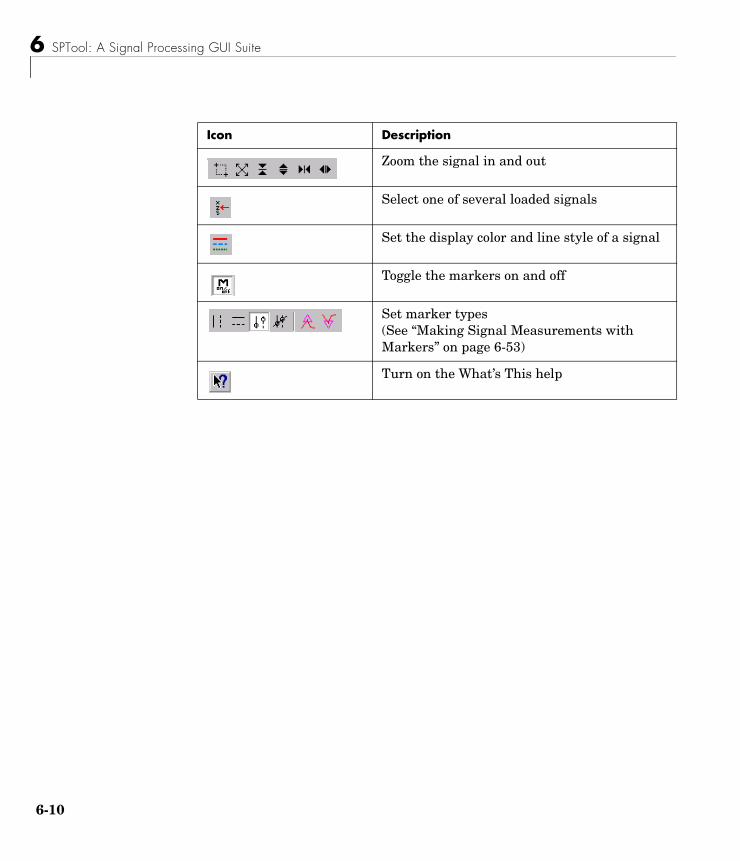
6 SPTool: A Signal Processing GUI Suite
6-1
Zoom the signal in and out
Select one of several loaded signals
Set the display color and line style of a signal
Toggle the markers on and off
Set marker types (See “Making Signal Measurements with Markers” on page 6-53)
Turn on the What’s This help
Icon Description
0
Filter Designer
Filter DesignerThe Filter Designer provides an interactive graphical environment for the design of digital IIR and FIR filters based on specifications that you enter on a magnitude or pole-zero plot.
Note You can also use the Filter Design and Analysis Tool (FDATool) described in Chapter 5, “FDATool: A Filter Design and Analysis GUI” for filter design and analysis.
Filter TypesYou can design filters of the following types using the Filter Designer:
• Bandpass
• Lowpass
• Bandstop
• Highpass
FIR Filter Methods You can use the following filter methods to design FIR filters:
• Equiripple
• Least squares
• Window
IIR Filter MethodsYou can use the following filter methods to design IIR filters:
• Butterworth
• Chebyshev Type I
• Chebyshev Type II
• Elliptic
6-11
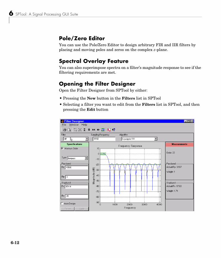
6 SPTool: A Signal Processing GUI Suite
6-1
Pole/Zero EditorYou can use the Pole/Zero Editor to design arbitrary FIR and IIR filters by placing and moving poles and zeros on the complex z-plane.
Spectral Overlay FeatureYou can also superimpose spectra on a filter’s magnitude response to see if the filtering requirements are met.
Opening the Filter DesignerOpen the Filter Designer from SPTool by either:
• Pressing the New button in the Filters list in SPTool
• Selecting a filter you want to edit from the Filters list in SPTool, and then pressing the Edit button
2
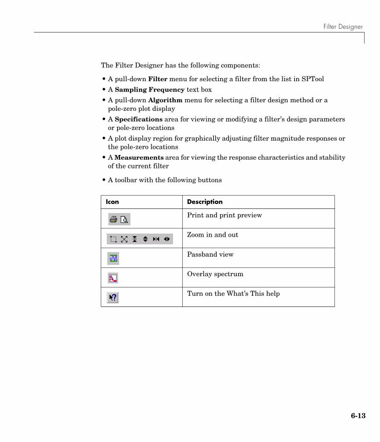
Filter Designer
The Filter Designer has the following components:
• A pull-down Filter menu for selecting a filter from the list in SPTool
• A Sampling Frequency text box
• A pull-down Algorithm menu for selecting a filter design method or a pole-zero plot display
• A Specifications area for viewing or modifying a filter’s design parameters or pole-zero locations
• A plot display region for graphically adjusting filter magnitude responses or the pole-zero locations
• A Measurements area for viewing the response characteristics and stability of the current filter
• A toolbar with the following buttons
Icon Description
Print and print preview
Zoom in and out
Passband view
Overlay spectrum
Turn on the What’s This help
6-13
6 SPTool: A Signal Processing GUI Suite
6-1
Filter Visualization ToolYou can use the Filter Visualization Tool (fvtool) to analyze the following response characteristics of selected filters:
• Magnitude response
• Phase response
• Impulse response
• Step response
• Group delay
• Phase delay
• Pole and zero locations
• Detailed filter information
FVTool also provides features for
• Overlaying filter responses
• Zooming
• Measuring filter responses
• Modifying display parameters such as frequency ranges or magnitude units
If you start FVTool by clicking the SPTool Filter View button, that FVTool is linked to SPTool. Any changes made in SPTool to the filter are immediately reflected in FVTool. The FVTool title bar includes “SPTool” to indicate the link.
If you start an FVTool by clicking the New button or by selecting File-->New from within FVTool, that FVTool is a stand-alone version and is not linked to SPTool.
Note Every time you click the Filter View button a new, linked FVTool starts. This allows you to view multiple analyses simultaneously.
Opening the Filter Visualization ToolYou open FVTool from SPTool as follows.
4
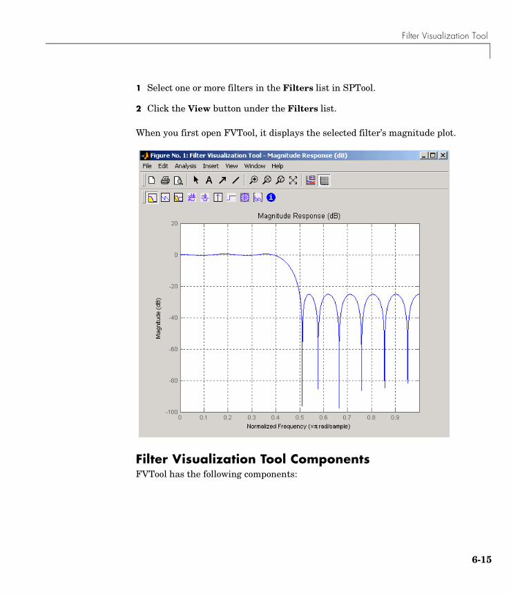
Filter Visualization Tool
1 Select one or more filters in the Filters list in SPTool.
2 Click the View button under the Filters list.
When you first open FVTool, it displays the selected filter’s magnitude plot.
Filter Visualization Tool ComponentsFVTool has the following components:
6-15
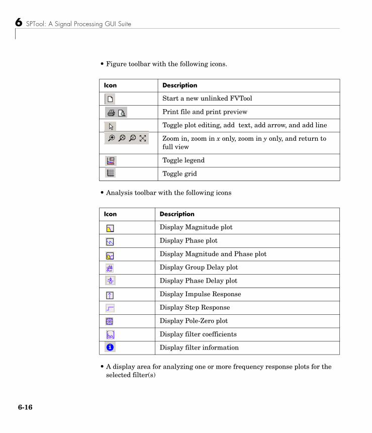
6 SPTool: A Signal Processing GUI Suite
6-1
• Figure toolbar with the following icons.
• Analysis toolbar with the following icons
• A display area for analyzing one or more frequency response plots for the selected filter(s)
Icon Description
Start a new unlinked FVTool
Print file and print preview
Toggle plot editing, add text, add arrow, and add line
Zoom in, zoom in x only, zoom in y only, and return to full view
Toggle legend
Toggle grid
Icon Description
Display Magnitude plot
Display Phase plot
Display Magnitude and Phase plot
Display Group Delay plot
Display Phase Delay plot
Display Impulse Response
Display Step Response
Display Pole-Zero plot
Display filter coefficients
Display filter information
6
Filter Visualization Tool
Using Data MarkersIn FVTool, you can use data markers to display information on particular points in the response plot(s). See “Data Markers” in the FDATool online help more information.
Analysis ParametersIn the plot area of any filter response plot, right-click and select Analysis Parameters to display details about the displayed plot. See “Analysis Parameters” in the FDATool online help for more information.
You can change any parameter in a linked FVTool, except the sampling frequency. You can only change the sampling frequency using Sampling Frequency in the SPTool Edit menu or the SPTool Filters Edit button.
6-17
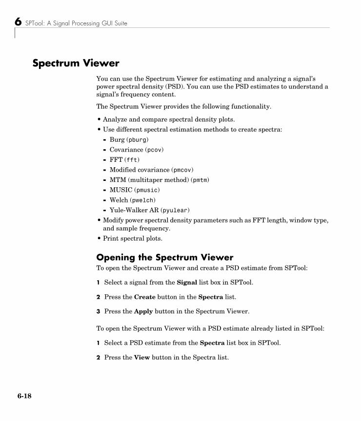
6 SPTool: A Signal Processing GUI Suite
6-1
Spectrum ViewerYou can use the Spectrum Viewer for estimating and analyzing a signal’s power spectral density (PSD). You can use the PSD estimates to understand a signal’s frequency content.
The Spectrum Viewer provides the following functionality.
• Analyze and compare spectral density plots.
• Use different spectral estimation methods to create spectra:
- Burg (pburg)
- Covariance (pcov)
- FFT (fft)
- Modified covariance (pmcov)
- MTM (multitaper method) (pmtm)
- MUSIC (pmusic)
- Welch (pwelch)
- Yule-Walker AR (pyulear)
• Modify power spectral density parameters such as FFT length, window type, and sample frequency.
• Print spectral plots.
Opening the Spectrum ViewerTo open the Spectrum Viewer and create a PSD estimate from SPTool:
1 Select a signal from the Signal list box in SPTool.
2 Press the Create button in the Spectra list.
3 Press the Apply button in the Spectrum Viewer.
To open the Spectrum Viewer with a PSD estimate already listed in SPTool:
1 Select a PSD estimate from the Spectra list box in SPTool.
2 Press the View button in the Spectra list.
8
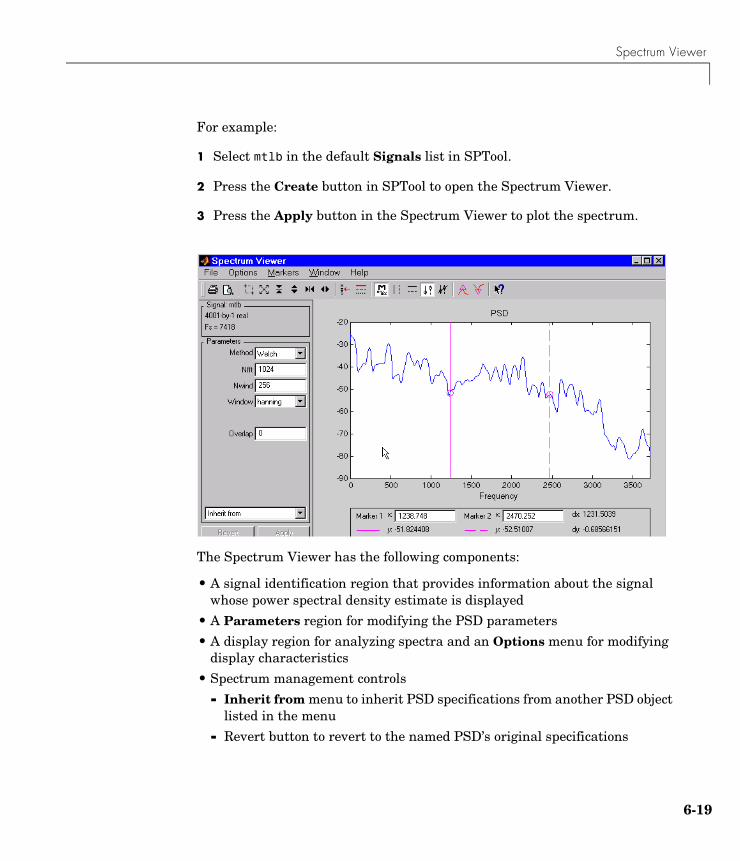
Spectrum Viewer
For example:
1 Select mtlb in the default Signals list in SPTool.
2 Press the Create button in SPTool to open the Spectrum Viewer.
3 Press the Apply button in the Spectrum Viewer to plot the spectrum.
The Spectrum Viewer has the following components:
• A signal identification region that provides information about the signal whose power spectral density estimate is displayed
• A Parameters region for modifying the PSD parameters
• A display region for analyzing spectra and an Options menu for modifying display characteristics
• Spectrum management controls
- Inherit from menu to inherit PSD specifications from another PSD object listed in the menu
- Revert button to revert to the named PSD’s original specifications
6-19
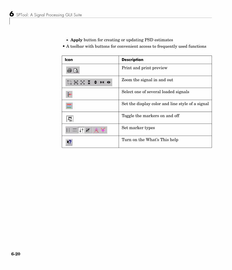
6 SPTool: A Signal Processing GUI Suite
6-2
- Apply button for creating or updating PSD estimates
• A toolbar with buttons for convenient access to frequently used functions
Icon Description
Print and print preview
Zoom the signal in and out
Select one of several loaded signals
Set the display color and line style of a signal
Toggle the markers on and off
Set marker types
Turn on the What’s This help
0
Filtering and Analysis of Noise
Filtering and Analysis of NoiseThe following sections provide an example of using the GUI-based interactive tools to:
• Design and implement an FIR bandpass digital filter
• Apply the filter to a noisy signal
• Analyze signals and their spectra
The steps include:
1 Creating a noisy signal in the MATLAB workspace and importing it into SPTool
2 Designing a bandpass filter using the Filter Designer
3 Applying the filter to the original noise signal to create a bandlimited noise signal
4 Comparing the time domain information of the original and filtered signals using the Signal Browser
5 Comparing the spectra of both signals using the Spectrum Viewer
Step 1: Importing a Signal into SPToolTo import a signal into SPTool from the workspace or disk, the signal must be either:
• A special MATLAB signal structure, such as that saved from a previous SPTool session
• A signal created as a variable (vector or matrix) in the MATLAB workspace
For this example, create a new signal at the command line and then import it as a structure into SPTool:
1 Create a random signal in the MATLAB workspace by typing
randn('state',0);x = randn(5000,1);
6-21
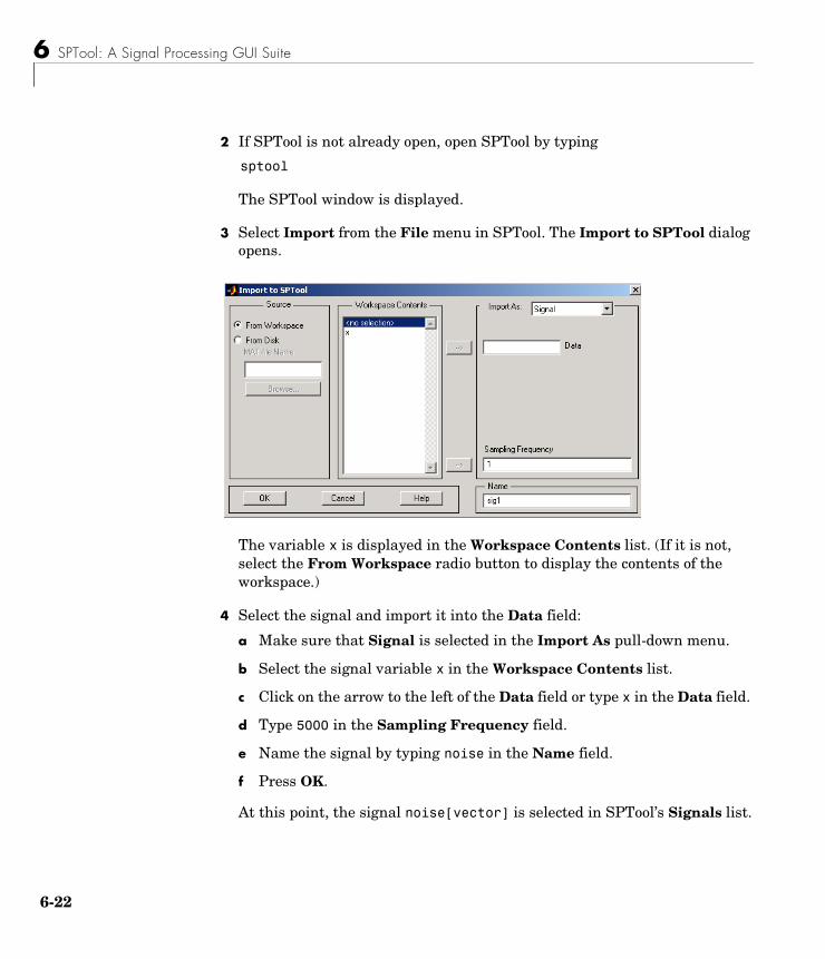
6 SPTool: A Signal Processing GUI Suite
6-2
2 If SPTool is not already open, open SPTool by typing
sptool
The SPTool window is displayed.
3 Select Import from the File menu in SPTool. The Import to SPTool dialog opens.
The variable x is displayed in the Workspace Contents list. (If it is not, select the From Workspace radio button to display the contents of the workspace.)
4 Select the signal and import it into the Data field:
a Make sure that Signal is selected in the Import As pull-down menu.
b Select the signal variable x in the Workspace Contents list.
c Click on the arrow to the left of the Data field or type x in the Data field.
d Type 5000 in the Sampling Frequency field.
e Name the signal by typing noise in the Name field.
f Press OK.
At this point, the signal noise[vector] is selected in SPTool’s Signals list.
2
Filtering and Analysis of Noise
Note You can import filters and spectra into SPTool in much the same way as you import signals. See “Importing Filters and Spectra into SPTool” on page 6-40 for specific details.
You can also import signals from MAT-files on your disk, rather than from the workspace. See “Loading Variables from the Disk” on page 6-44 for more information.
Type help sptool for information about importing from the command line.
Step 2: Designing a FilterYou can import an existing filter into SPTool, or you can design and edit a new filter using the Filter Designer.
In this example:
1 Open a default filter in the Filter Designer.
2 Specify an equiripple bandpass FIR filter.
Opening the Filter DesignerTo open the Filter Designer, press the New button in SPTool. This opens the Filter Designer with a default filter named filt1.
Specifying the Bandpass FilterDesign an equiripple bandpass FIR filter with the following characteristics:
• Sampling frequency of 5000 Hz
• Stopband frequency ranges of [0 500] Hz and [1500 2500] Hz
• Passband frequency range of [750 1250] Hz
• Ripple in the passband of 0.01 dB
• Stopband attenuation of 75 dB
To modify your filter in the Filter Designer to meet these specifications:
6-23
6 SPTool: A Signal Processing GUI Suite
6-2
1 Change the filter sampling frequency to 5000 by entering this value in the Sampling Frequency text box.
2 Select Equiripple FIR from the Algorithm list.
3 Select bandpass from the Type list.
4 Set the passband edge frequencies by entering 750 for Fp1 and 1250 for Fp2.
5 Set the stopband edge frequencies by entering 500 for Fs1 and 1500 for Fs2.
6 Type 0.01 into the Rp field and 75 into the Rs field.
Rp sets the maximum passband ripple and Rs sets the stopband attenuation for the filter.
7 Press the Apply button to design the new filter.When the new filter is designed, the magnitude response of the filter is displayed with a solid line in the display region.
4
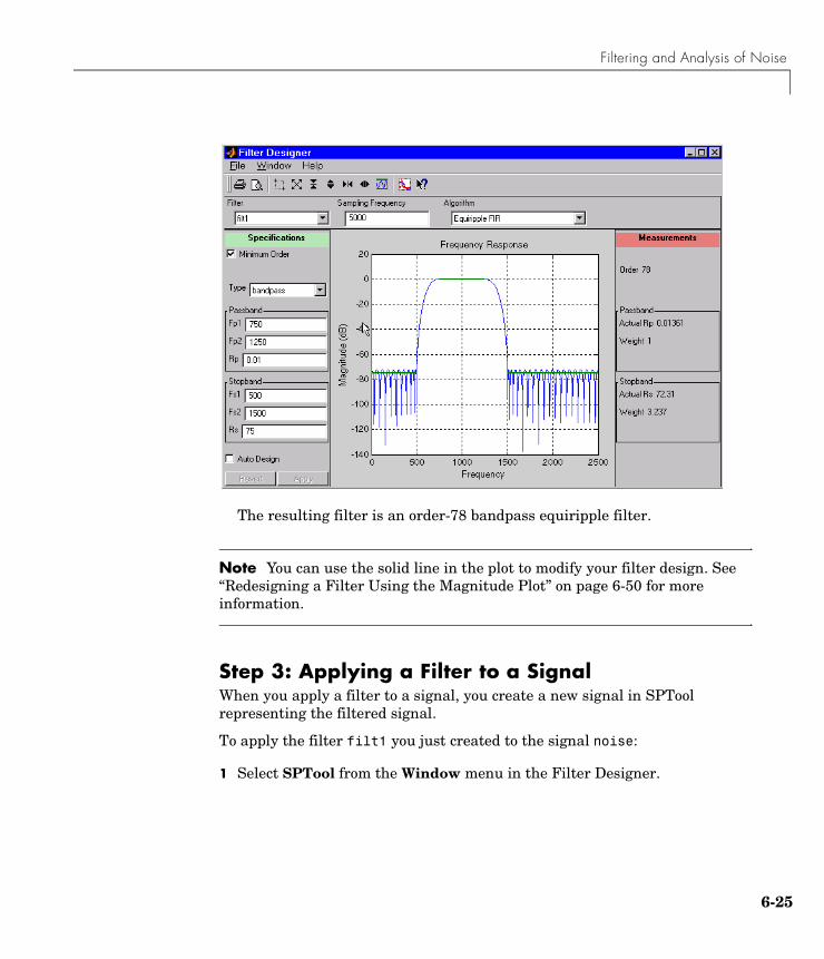
Filtering and Analysis of Noise
The resulting filter is an order-78 bandpass equiripple filter.
Note You can use the solid line in the plot to modify your filter design. See “Redesigning a Filter Using the Magnitude Plot” on page 6-50 for more information.
Step 3: Applying a Filter to a SignalWhen you apply a filter to a signal, you create a new signal in SPTool representing the filtered signal.
To apply the filter filt1 you just created to the signal noise:
1 Select SPTool from the Window menu in the Filter Designer.
6-25
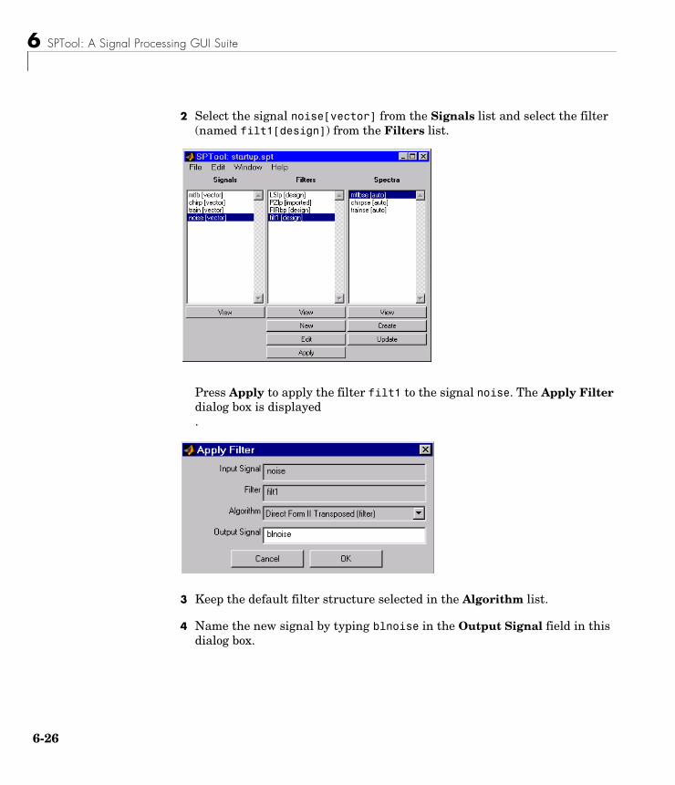
6 SPTool: A Signal Processing GUI Suite
6-2
2 Select the signal noise[vector] from the Signals list and select the filter (named filt1[design]) from the Filters list.
Press Apply to apply the filter filt1 to the signal noise. The Apply Filter dialog box is displayed.
3 Keep the default filter structure selected in the Algorithm list.
4 Name the new signal by typing blnoise in the Output Signal field in this dialog box.
6
Filtering and Analysis of Noise
5 Press OK to close the Apply Filter dialog box.
The filter is applied to the selected signal and the filtered signal blnoise[vector] is listed in the Signals list in SPTool.
Step 4: Analyzing a SignalYou can analyze and print signals using the Signal Browser. You can also play the signals if your computer has audio output capabilities.
For example, compare the signal noise to the filtered signal blnoise:
1 Shift+click on the noise and blnoise signals in the Signals list of SPTool to select both signals.
2 Press the View button under the Signals list.
The Signal Browser is activated and both signals are displayed in the display region. (The names of both signals are shown above the display region.) Initially, the original noise signal covers up the bandlimited blnoise signal.
3 Push the selection button on the toolbar, , to select the blnoise signal.
The display area is updated. Now you can see the blnoise signal superimposed on top of the noise signal. The signals are displayed in different colors in both the display region and the panner. You can change the color of the selected signal using the Line Properties button on the toolbar, .
6-27
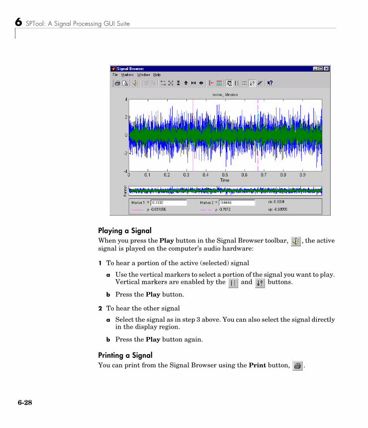
6 SPTool: A Signal Processing GUI Suite
6-2
Playing a SignalWhen you press the Play button in the Signal Browser toolbar, , the active signal is played on the computer’s audio hardware:
1 To hear a portion of the active (selected) signal
a Use the vertical markers to select a portion of the signal you want to play. Vertical markers are enabled by the and buttons.
b Press the Play button.
2 To hear the other signal
a Select the signal as in step 3 above. You can also select the signal directly in the display region.
b Press the Play button again.
Printing a SignalYou can print from the Signal Browser using the Print button, .
8
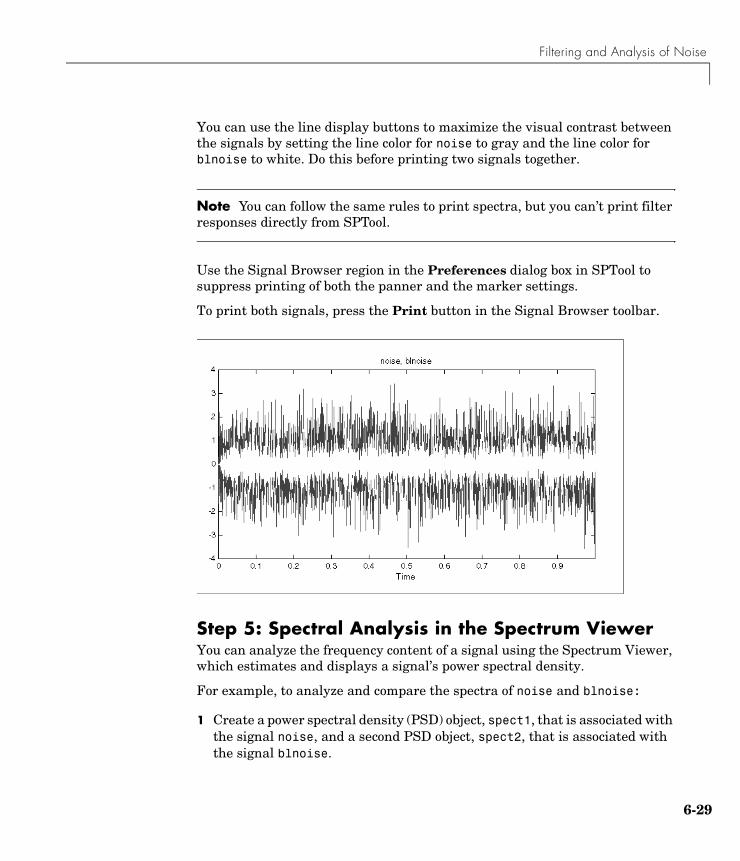
Filtering and Analysis of Noise
You can use the line display buttons to maximize the visual contrast between the signals by setting the line color for noise to gray and the line color for blnoise to white. Do this before printing two signals together.
Note You can follow the same rules to print spectra, but you can’t print filter responses directly from SPTool.
Use the Signal Browser region in the Preferences dialog box in SPTool to suppress printing of both the panner and the marker settings.
To print both signals, press the Print button in the Signal Browser toolbar.
Step 5: Spectral Analysis in the Spectrum ViewerYou can analyze the frequency content of a signal using the Spectrum Viewer, which estimates and displays a signal’s power spectral density.
For example, to analyze and compare the spectra of noise and blnoise:
1 Create a power spectral density (PSD) object, spect1, that is associated with the signal noise, and a second PSD object, spect2, that is associated with the signal blnoise.
6-29
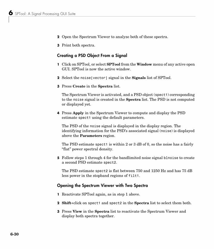
6 SPTool: A Signal Processing GUI Suite
6-3
2 Open the Spectrum Viewer to analyze both of these spectra.
3 Print both spectra.
Creating a PSD Object From a Signal
1 Click on SPTool, or select SPTool from the Window menu of any active open GUI. SPTool is now the active window.
2 Select the noise[vector] signal in the Signals list of SPTool.
3 Press Create in the Spectra list.
The Spectrum Viewer is activated, and a PSD object (spect1) corresponding to the noise signal is created in the Spectra list. The PSD is not computed or displayed yet.
4 Press Apply in the Spectrum Viewer to compute and display the PSD estimate spect1 using the default parameters.
The PSD of the noise signal is displayed in the display region. The identifying information for the PSD’s associated signal (noise) is displayed above the Parameters region.
The PSD estimate spect1 is within 2 or 3 dB of 0, so the noise has a fairly “flat” power spectral density.
5 Follow steps 1 through 4 for the bandlimited noise signal blnoise to create a second PSD estimate spect2.
The PSD estimate spect2 is flat between 750 and 1250 Hz and has 75 dB less power in the stopband regions of filt1.
Opening the Spectrum Viewer with Two Spectra
1 Reactivate SPTool again, as in step 1 above.
2 Shift+click on spect1 and spect2 in the Spectra list to select them both.
3 Press View in the Spectra list to reactivate the Spectrum Viewer and display both spectra together.
0
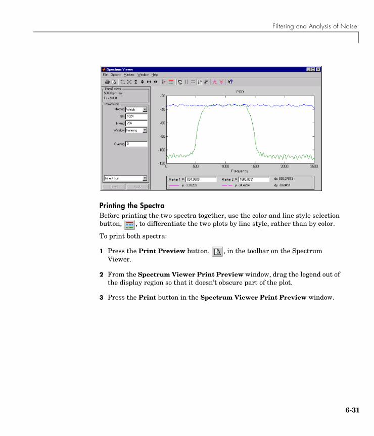
Filtering and Analysis of Noise
Printing the SpectraBefore printing the two spectra together, use the color and line style selection button, , to differentiate the two plots by line style, rather than by color.
To print both spectra:
1 Press the Print Preview button, , in the toolbar on the Spectrum Viewer.
2 From the Spectrum Viewer Print Preview window, drag the legend out of the display region so that it doesn’t obscure part of the plot.
3 Press the Print button in the Spectrum Viewer Print Preview window.
6-31
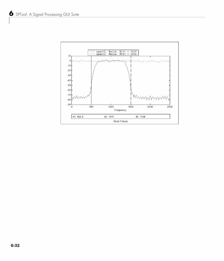
6 SPTool: A Signal Processing GUI Suite
6-3
2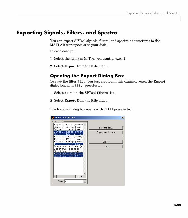
Exporting Signals, Filters, and Spectra
Exporting Signals, Filters, and SpectraYou can export SPTool signals, filters, and spectra as structures to the MATLAB workspace or to your disk.
In each case you:
1 Select the items in SPTool you want to export.
2 Select Export from the File menu.
Opening the Export Dialog BoxTo save the filter filt1 you just created in this example, open the Export dialog box with filt1 preselected:
1 Select filt1 in the SPTool Filters list.
2 Select Export from the File menu.
The Export dialog box opens with filt1 preselected.
6-33
6 SPTool: A Signal Processing GUI Suite
6-3
Exporting a Filter to the MATLAB WorkspaceTo export the filter filt1 to the MATLAB workspace:
1 Select filt1 from the Export List and deselect all other items using Ctrl+click.
2 Press the Export to Workspace button.
4
Accessing Filter Parameters
Accessing Filter ParametersYou can access filter parameters in the following two ways.
• “Accessing Filter Parameters in a Saved Filter”
• “Accessing Parameters in a Saved Spectrum”
Accessing Filter Parameters in a Saved FilterThe MATLAB structures created by SPTool have several associated fields, many of which are also MATLAB structures. See the MATLAB documentation for general information about MATLAB structures.
For example, after exporting a filter filt1 to the MATLAB workspace, type
filt1
to display the fields of the MATLAB filter structure. The tf, Fs, and specs fields of the structure contain the information that describes the filter.
The tf Field: Accessing Filter CoefficientsThe tf field is a structure containing the transfer function representation of the filter. Use this field to obtain the filter coefficients;
• filt1.tf.num contains the numerator coefficients.
• filt1.tf.den contains the denominator coefficients.
The vectors contained in these structures represent polynomials in descending powers of z. The numerator and denominator polynomials are used to specify the transfer function
where:
• b is a vector containing the coefficients from the tf.num field.
• a is a vector containing the coefficients from the tf.den field.
• m is the numerator order.
• n is the denominator order.
H z( )B z( )A z( )----------- b 1( ) b 2( )z 1– b nb 1+( )z m–+ + +
a 1( ) a 2( )z 1– a na 1+( )z n–+ + +-----------------------------------------------------------------------------------------= =
6-35
6 SPTool: A Signal Processing GUI Suite
6-3
You can change the filter representation from the default transfer function to another form by using the tf2ss or tf2zp functions.
The Fs Field: Accessing Filter Sample FrequencyThe Fs field contains the sampling frequency of the filter in hertz.
The specs Field: Accessing other Filter ParametersThe specs field is a structure containing parameters that you specified for the filter design. The first field, specs.currentModule, contains a string representing the most recent design method selected from the Filter Designer’s Algorithm list before you exported the filter. The possible contents of the currentModule field and the corresponding design methods are shown below.
Following the specs.currentModule field, there may be up to seven additional fields, with labels such as specs.fdremez, specs.fdfirls, etc. The design specifications for the most recently exported filter are contained in the field whose label matches the currentModule string. For example, if the specs structure is
filt1.specs
anscurrentModule: 'fdremez'fdremez: [1x1 struct]
Contents of the currentModule field Design Method
fdbutter Butterworth IIR
fdcheby1 Chebyshev Type I IIR
fdcheby2 Chebyshev Type II IIR
fdellip Elliptic IIR
fdfirls Least Squares FIR
fdkaiser Kaiser Window FIR
fdremez Equiripple FIR
6
Accessing Filter Parameters
the filter specifications are contained in the fdremez field, which is itself a data structure.
The specifications include the parameter values from the Specifications region of the Filter Designer, such as band edges and filter order. For example, the filter above has the following specifications stored in filt1.specs.fdremez:
filt1.specs.fdremez
ans = setOrderFlag: 0 type: 3 f: [0 0.2000 0.3000 0.5000 0.6000 1] m: [6x1 double] Rp: 0.0100 Rs: 75 wt: [3.2371 1 3.2371] order: 78
Because certain filter parameters are unique to a particular design, this structure has a different set of fields for each filter design.
The table below describes the possible fields associated with the filter design specification field (the specs field) that can appear in the exported structure.
Parameter Description
Beta Kaiser window β parameter.
f Contains a vector of band-edge frequencies, normalized so that 1 Hz corresponds to half the sample frequency.
Fpass Passband cutoff frequencies. Scalar for lowpass and highpass designs, two-element vector for bandpass and bandstop designs.
Fstop Stopband cutoff frequencies. Scalar for lowpass and highpass designs, two-element vector for bandpass and bandstop designs.
6-37
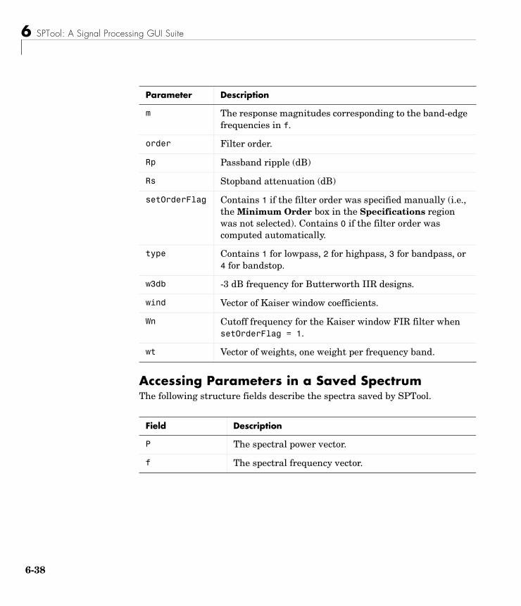
6 SPTool: A Signal Processing GUI Suite
6-3
Accessing Parameters in a Saved SpectrumThe following structure fields describe the spectra saved by SPTool.
m The response magnitudes corresponding to the band-edge frequencies in f.
order Filter order.
Rp Passband ripple (dB)
Rs Stopband attenuation (dB)
setOrderFlag Contains 1 if the filter order was specified manually (i.e., the Minimum Order box in the Specifications region was not selected). Contains 0 if the filter order was computed automatically.
type Contains 1 for lowpass, 2 for highpass, 3 for bandpass, or 4 for bandstop.
w3db -3 dB frequency for Butterworth IIR designs.
wind Vector of Kaiser window coefficients.
Wn Cutoff frequency for the Kaiser window FIR filter when setOrderFlag = 1.
wt Vector of weights, one weight per frequency band.
Field Description
P The spectral power vector.
f The spectral frequency vector.
Parameter Description
8
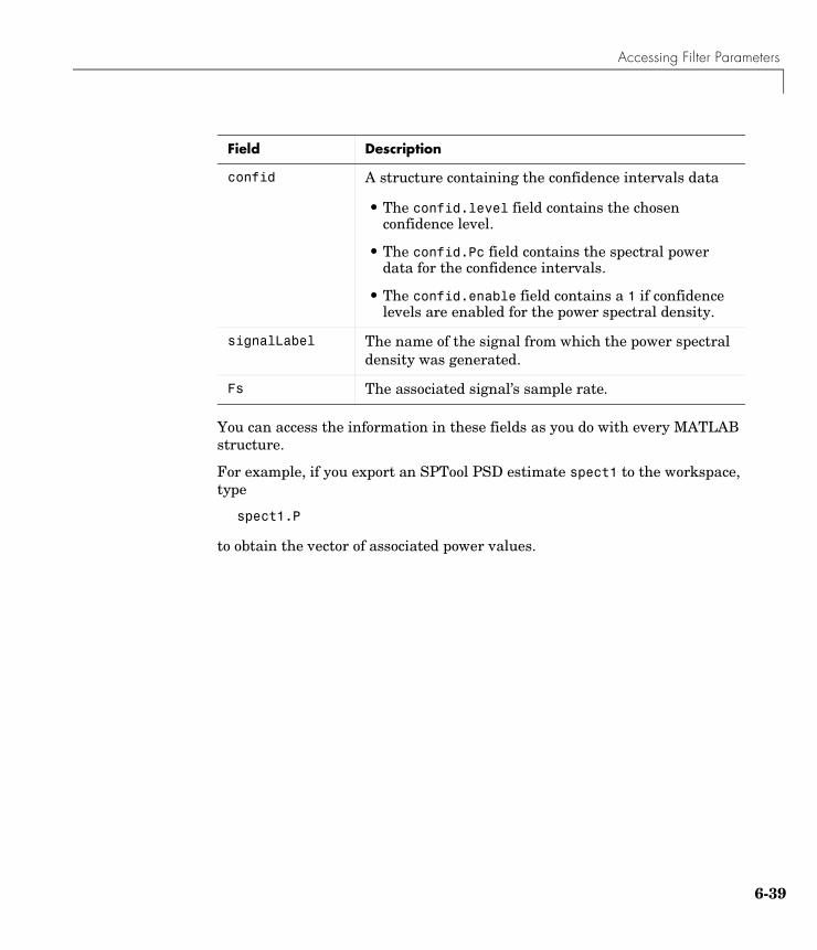
Accessing Filter Parameters
You can access the information in these fields as you do with every MATLAB structure.
For example, if you export an SPTool PSD estimate spect1 to the workspace, type
spect1.P
to obtain the vector of associated power values.
confid A structure containing the confidence intervals data
• The confid.level field contains the chosen confidence level.
• The confid.Pc field contains the spectral power data for the confidence intervals.
• The confid.enable field contains a 1 if confidence levels are enabled for the power spectral density.
signalLabel The name of the signal from which the power spectral density was generated.
Fs The associated signal’s sample rate.
Field Description
6-39
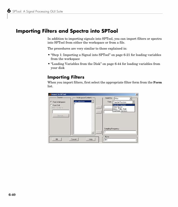
6 SPTool: A Signal Processing GUI Suite
6-4
Importing Filters and Spectra into SPToolIn addition to importing signals into SPTool, you can import filters or spectra into SPTool from either the workspace or from a file.
The procedures are very similar to those explained in:
• “Step 1: Importing a Signal into SPTool” on page 6-21 for loading variables from the workspace
• “Loading Variables from the Disk” on page 6-44 for loading variables from your disk
Importing FiltersWhen you import filters, first select the appropriate filter form from the Form list.
0
Importing Filters and Spectra into SPTool
For every filter you specify a variable name or a value for the filter’s sampling frequency in the Sampling Frequency field. Each filter form requires different variables.
Transfer FunctionFor Transfer Function, you specify the filter by its transfer function representation:
• The Numerator field specifies a variable name or value for the numerator coefficient vector b, which contains m+1 coefficients in descending powers of z.
• The Denominator field specifies a variable name or value for the denominator coefficient vector a, which contains n+1 coefficients in descending powers of z.
State SpaceFor State Space, you specify the filter by its state-space representation:
The A-Matrix, B-Matrix, C-Matrix, and D-Matrix fields specify a variable name or a value for each matrix in this system.
Zeros, Poles, GainFor Zeros, Poles, Gain, you specify the filter by its zero-pole-gain representation:
• The Zeros field specifies a variable name or value for the zeros vector z, which contains the locations of m zeros.
• The Poles field specifies a variable name or value for the zeros vector p, which contains the locations of n poles.
H z( )B z( )A z( )----------- b 1( ) b 2( )z 1– b m 1+( )z m–+ + +
a 1( ) a 2( )z 1– a n 1+( )z n–+ + +---------------------------------------------------------------------------------------= =
x· Ax Bu+=
y Cx Du+=
H z( )Z z( )P z( )---------- k z z 1( )–( ) z z 2( )–( ) z z m( )–( )
z p 1( )–( ) z p 2( )–( ) z p n( )–( )------------------------------------------------------------------------------------= =
6-41
6 SPTool: A Signal Processing GUI Suite
6-4
• The Gain field specifies a variable name or value for the gain k.
Second Order SectionsFor 2nd Order Sections you specify the filter by its second-order section representation:
The SOS Matrix field specifies a variable name or a value for the L-by-6 SOS matrix
whose rows contain the numerator and denominator coefficients bik and aik of the second-order sections of H(z).
Note If you import a filter that was not created in SPTool, you can only edit that filter using the Pole/Zero Editor.
H z( ) Hk z( )
k 1=
L
∏b0k b1kz 1– b2kz 2–+ +
1 a1kz 1– a2kz 2–+ +----------------------------------------------------------
k 1=
L
∏= =
sos
b01 b11 b21 1 a11 a21
b02 b12 b22 1 a12 a22
b0L b1L b2L 1 a1L a2L
=
2
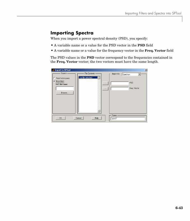
Importing Filters and Spectra into SPTool
Importing SpectraWhen you import a power spectral density (PSD), you specify:
• A variable name or a value for the PSD vector in the PSD field
• A variable name or a value for the frequency vector in the Freq. Vector field
The PSD values in the PSD vector correspond to the frequencies contained in the Freq. Vector vector; the two vectors must have the same length.
6-43

6 SPTool: A Signal Processing GUI Suite
6-4
Loading Variables from the DiskTo import variables representing signals, filters, or spectra from a MAT-file on your disk;
1 Select the From Disk radio button and do either of the following:
- Type the name of the file you want to import into the MAT-file Name field and press either the Tab or the Enter key on your keyboard.
- Select Browse, and then find and select the file you want to import using the Select File to Open dialog. Press OK to close that dialog.
In either case, all variables in the MAT-file you selected are displayed in the File Contents list.
2 Select the variables to be imported into SPTool.
You can now import one or more variables from the File Contents list into SPTool, as long as these variables are scalars, vectors, or matrices.
4
Selecting Signals, Filters, and Spectra in SPTool
Selecting Signals, Filters, and Spectra in SPToolAll signals, filters, or spectra listed in SPTool exist as special MATLAB structures. You can bring data representing signals, filters, or spectra into SPTool from the MATLAB workspace. In general, you can select one or several items in a given list box. An item is selected when it is highlighted.
The Signals list shows all vector and array signals in the current SPTool session.
The Filters list shows all designed and imported filters in the current SPTool session.
The Spectra list shows all spectra in the current SPTool session.
You can select a single data object in a list, a range of data objects in a list, or multiple separate data objects in a list. You can also have data objects simultaneously selected in different lists:
• To select a single item, click on it. All other items in that list box become deselected.
• To add or remove a range of items, Shift+click on the items at the top and bottom of the section of the list that you want to add. You can also drag your mouse pointer to select these items.
• To add a single data object to a selection or remove a single data object from a multiple selection, Ctrl+click on the object.
6-45
6 SPTool: A Signal Processing GUI Suite
6-4
Editing Signals, Filters, or Spectra in SPToolYou can edit selected items in SPTool by:
1 Selecting the names of the signals, filters, or spectra you want to edit.
2 Selecting the appropriate Edit menu item:
- Duplicate to copy an item in an SPTool list
- Clear to delete an item in an SPTool list
- Name to rename an item in an SPTool list
- Sampling Frequency to modify the sampling frequency associated with either a signal (and its associated spectra) or filter in an SPTool list
The pull-down menu next to each menu item shows the names of all selected items.
You can also edit the following signal characteristics by right-clicking in the display region of the Signal Browser, the Filter Visualization Tool, or the Spectrum Viewer:
• The signal name
• The sampling frequency
• The line style properties
Note If you modify the sampling frequency associated with a signal’s spectrum using the right-click menu on the Spectrum Viewer display region, the sampling frequency of the associated signal is automatically updated.
6

Designing a Filter with the Pole/Zero Editor
Designing a Filter with the Pole/Zero EditorTo design a filter transfer function using the Filter Designer Pole/Zero Editor:
1 Select the Pole/Zero Editor option from the Algorithm list to open the Pole/Zero Editor in the Filter Designer display.
2 Enter the desired filter gain in the Gain edit box.
3 Select a pole or zero (or conjugate pair) by selecting one of the (pole) or (zero) symbols on the plot.
4 Choose the coordinates to work in by specifying Polar or Rectangular from the Coordinates list.
5 Specify the new location(s) of the selected pole, zero, or conjugate pair by typing values into the Mag and Angle fields (for angular coordinates) or X and Y (for rectangular coordinates) fields. Alternatively, position the poles and zeros by dragging the and symbols.
6 Use the Conjugate pair check box to create a conjugate pair from a lone pole or zero, or to break a conjugate pair into two individual poles or zeros.
Design a new filter or edit an existing filter in the same way.
Note Keep the Filter Visualization Tool (FVTool) open while designing a filter with the Pole/Zero Editor. Any changes that you make to the filter transfer function in the Pole/Zero Editor are then simultaneously reflected in the response plots of FVTool.
6-47
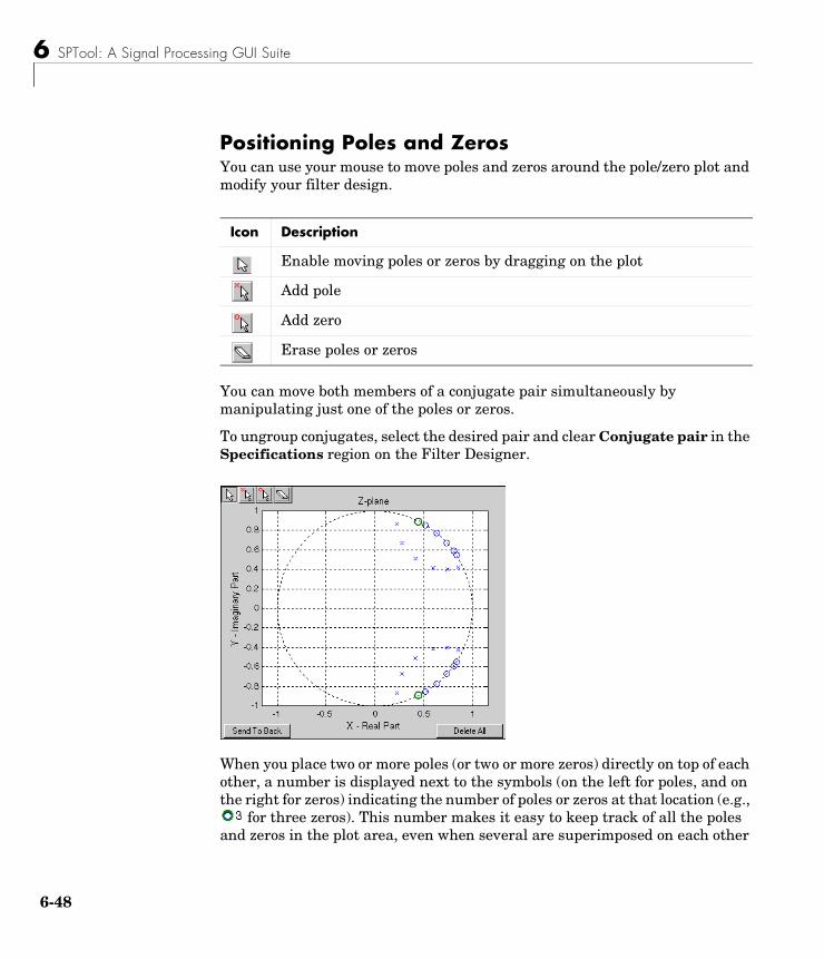
6 SPTool: A Signal Processing GUI Suite
6-4
Positioning Poles and ZerosYou can use your mouse to move poles and zeros around the pole/zero plot and modify your filter design.
You can move both members of a conjugate pair simultaneously by manipulating just one of the poles or zeros.
To ungroup conjugates, select the desired pair and clear Conjugate pair in the Specifications region on the Filter Designer.
When you place two or more poles (or two or more zeros) directly on top of each other, a number is displayed next to the symbols (on the left for poles, and on the right for zeros) indicating the number of poles or zeros at that location (e.g.,
for three zeros). This number makes it easy to keep track of all the poles and zeros in the plot area, even when several are superimposed on each other
Icon Description
Enable moving poles or zeros by dragging on the plot
Add pole
Add zero
Erase poles or zeros
8
Designing a Filter with the Pole/Zero Editor
and are not visually differentiable. Note, however, that this number does not indicate the multiplicity of the poles or zeros to which it is attached.
To detect whether or not a set of poles or zeros are truly multiples, use the zoom tools to magnify the region around the poles or zeros in question. Because numerical limitations usually prevent any set of poles or zeros from sharing exactly the same value, at a high enough zoom level even truly multiple poles or zeros appear distinct from each other.
A common way to assess whether a particular group of poles or zeros contains multiples is by comparing the mutual proximity of the group members against a selected threshold value. As an example, the residuez function defines a pole or zero as being a multiple of another pole or zero if the absolute distance separating them is less than 0.1% of the larger pole or zero’s magnitude.
6-49
6 SPTool: A Signal Processing GUI Suite
6-5
Redesigning a Filter Using the Magnitude PlotAfter designing a filter in the Filter Designer, you can redesign it by dragging the specification lines on the magnitude plot. Use the specification lines to change passband ripple, stopband attenuation, and edge frequencies.
In the following example, create a Chebyshev filter and modify it by dragging the specification lines:
1 Select Chebyshev Type I IIR from the Algorithm menu.
2 Select highpass from the Type menu.
3 Type 2000 in the Sampling Frequency field.
4 Set the following parameters:
- Fp = 800
- Fs = 700
- Rp = 2.5
- Rs = 35
5 Select Minimum Order so the Filter Designer can calculate the lowest filter order that produces the desired characteristics.
6 Press Apply to compute the filter and update the response plot.
7 Position the cursor over the horizontal filter specification line for the stopband. This is the first (leftmost) horizontal specification line you see.
The cursor changes to the up/down drag indicator.
8 Drag the line until the Rs (stopband attenuation) field reads 100.
Note The Order value in the Measurements region changes because a higher filter order is needed to meet the new specifications.
0
Setting Preferences
Setting PreferencesUse Preferences from the SPTool File menu to customize displays and certain parameters for SPTool and its four component GUIs. The new settings are saved on disk and are used when you restart SPTool from MATLAB.
In the Preferences regions, you can:
• Select colors and markers for all displays.
• Select colors and line styles for displayed signals.
• Configure labels, and enable/disable markers, panner, and zoom in the Signal Browser.
• Configure display parameters, and enable/disable markers and zoom in the Spectrum Viewer.
• Specify FFT length, and enable/disable mouse zoom and grid in the Filter Designer.
• Enable/disable use of a default session file.
• Export filters for use with the Control System Toolbox.
• Enable/disable search for plug-ins at start-up.
Note You can set MATLAB preferences that affect the Filter Visualization Tool only from within FVTool by selecting Preferences from the File menu. You can set FVTool-specific preferences using the Analysis Parameters on the Analysis menu.
When you first select Preferences, the Preferences dialog box opens with Markers selected by default.
6-51
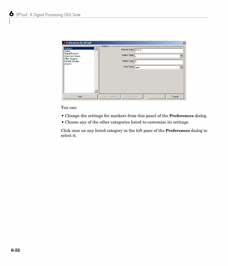
6 SPTool: A Signal Processing GUI Suite
6-5
You can:
• Change the settings for markers from this panel of the Preferences dialog.
• Choose any of the other categories listed to customize its settings.
Click once on any listed category in the left pane of the Preferences dialog to select it.
2

Making Signal Measurements with Markers
Making Signal Measurements with MarkersYou can use the markers on the Signal Browser or the Spectrum Viewer to make measurements on either of the following:
• A signal in the Signal Browser
• A power spectral density plotted in the Spectrum Viewer
The following marker buttons are included
.
To make a measurement:
1 Select a line to measure (or play, if you are in the Signal Browser).
2 Select one of the marker buttons to apply a marker to the displayed signal.
3 Position a marker in the main display area by grabbing it with your mouse and dragging:
Icon Description
Toggle markers on/off
Vertical markers
Horizontal markers
Vertical markers with tracking
Vertical markers with tracking and slope
Display peaks (local maxima)
Display valleys (local minima)
6-53
6 SPTool: A Signal Processing GUI Suite
6-5
a Select a marker setting. If you choose the Vertical, Track, or Slope buttons, you can drag a marker to the right or left. If you choose the Horizontal button, you can drag a marker up or down.
b Move the mouse over the marker (1 or 2) that you want to drag.
The hand cursor with the marker number inside it is displayed when your mouse passes over a marker.
c Drag the marker to where you want it on the signal.
As you drag a marker, the bottom of the Signal Browser shows the current position of both markers. Depending on which marker setting you select, some or all of the following fields are displayed—x1, y1, x2, y2, dx, dy, m. These fields are also displayed when you print from the Signal Browser, unless you suppress them.
You can also position a marker by typing its x1 and x2 or y1 and y2 values in the region at the bottom.
4
7
Function Reference
Functions — Categorical List (p. 7-2) Signal Toolbox functions arranged in categories
Functions — Alphabetical List (p. 7-17) Signal Toolbox functions arranged alphabetically

7 Function Reference
7-2
Functions — Categorical ListThis section contains brief descriptions of all functions in the Signal Processing Toolbox arranged by category.
“FIR Digital Filter Design”
“IIR Digital Filter Design”
“IIR FIlter Order Estimation”
“Filter Analysis”
“Filter Implementation”
“Analog Lowpass Filter Prototypes”
“Analog Filter Design”
“Analog Filter Transformation”
“Filter Discretization”
“Linear System Transformations”
“Windows”
“Transforms”
“Cepstral Analysis”
“Statistical Signal Processing and Spectral Analysis”
“Parametric Modeling”
“Linear Prediction”
“Multirate Signal Processing”
“Waveform Generation”
“Specialized Operations”
“Graphical User Interfaces”
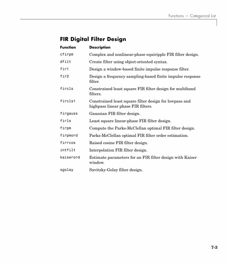
Functions — Categorical List
FIR Digital Filter DesignFunction Description
cfirpm Complex and nonlinear-phase equiripple FIR filter design.
dfilt Create filter using object-oriented syntax.
fir1 Design a window-based finite impulse response filter.
fir2 Design a frequency sampling-based finite impulse response filter.
fircls Constrained least square FIR filter design for multiband filters.
fircls1 Constrained least square filter design for lowpass and highpass linear phase FIR filters.
firgauss Gaussian FIR filter design.
firls Least square linear-phase FIR filter design.
firpm Compute the Parks-McClellan optimal FIR filter design.
firpmord Parks-McClellan optimal FIR filter order estimation.
firrcos Raised cosine FIR filter design.
intfilt Interpolation FIR filter design.
kaiserord Estimate parameters for an FIR filter design with Kaiser window.
sgolay Savitzky-Golay filter design.
7-3
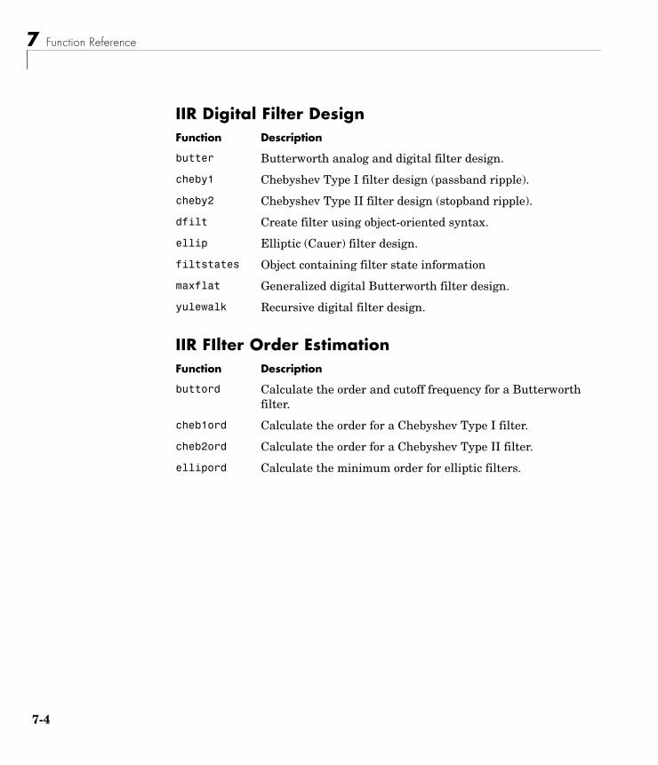
7 Function Reference
7-4
IIR Digital Filter Design
IIR FIlter Order Estimation
Function Description
butter Butterworth analog and digital filter design.
cheby1 Chebyshev Type I filter design (passband ripple).
cheby2 Chebyshev Type II filter design (stopband ripple).
dfilt Create filter using object-oriented syntax.
ellip Elliptic (Cauer) filter design.
filtstates Object containing filter state information
maxflat Generalized digital Butterworth filter design.
yulewalk Recursive digital filter design.
Function Description
buttord Calculate the order and cutoff frequency for a Butterworth filter.
cheb1ord Calculate the order for a Chebyshev Type I filter.
cheb2ord Calculate the order for a Chebyshev Type II filter.
ellipord Calculate the minimum order for elliptic filters.
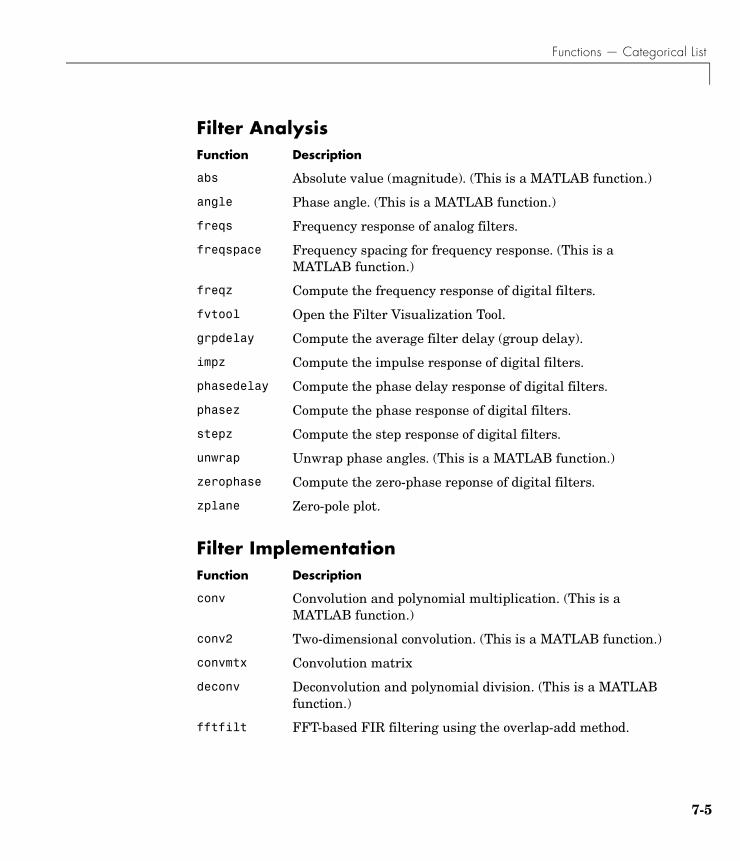
Functions — Categorical List
Filter Analysis
Filter Implementation
Function Description
abs Absolute value (magnitude). (This is a MATLAB function.)
angle Phase angle. (This is a MATLAB function.)
freqs Frequency response of analog filters.
freqspace Frequency spacing for frequency response. (This is a MATLAB function.)
freqz Compute the frequency response of digital filters.
fvtool Open the Filter Visualization Tool.
grpdelay Compute the average filter delay (group delay).
impz Compute the impulse response of digital filters.
phasedelay Compute the phase delay response of digital filters.
phasez Compute the phase response of digital filters.
stepz Compute the step response of digital filters.
unwrap Unwrap phase angles. (This is a MATLAB function.)
zerophase Compute the zero-phase reponse of digital filters.
zplane Zero-pole plot.
Function Description
conv Convolution and polynomial multiplication. (This is a MATLAB function.)
conv2 Two-dimensional convolution. (This is a MATLAB function.)
convmtx Convolution matrix
deconv Deconvolution and polynomial division. (This is a MATLAB function.)
fftfilt FFT-based FIR filtering using the overlap-add method.
7-5
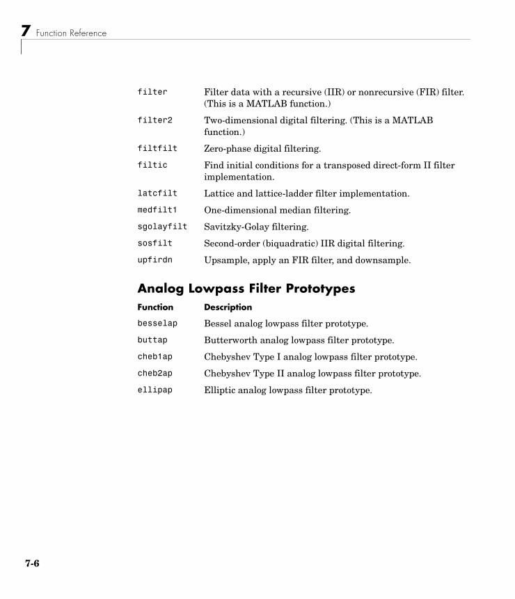
7 Function Reference
7-6
Analog Lowpass Filter Prototypes
filter Filter data with a recursive (IIR) or nonrecursive (FIR) filter. (This is a MATLAB function.)
filter2 Two-dimensional digital filtering. (This is a MATLAB function.)
filtfilt Zero-phase digital filtering.
filtic Find initial conditions for a transposed direct-form II filter implementation.
latcfilt Lattice and lattice-ladder filter implementation.
medfilt1 One-dimensional median filtering.
sgolayfilt Savitzky-Golay filtering.
sosfilt Second-order (biquadratic) IIR digital filtering.
upfirdn Upsample, apply an FIR filter, and downsample.
Function Description
besselap Bessel analog lowpass filter prototype.
buttap Butterworth analog lowpass filter prototype.
cheb1ap Chebyshev Type I analog lowpass filter prototype.
cheb2ap Chebyshev Type II analog lowpass filter prototype.
ellipap Elliptic analog lowpass filter prototype.
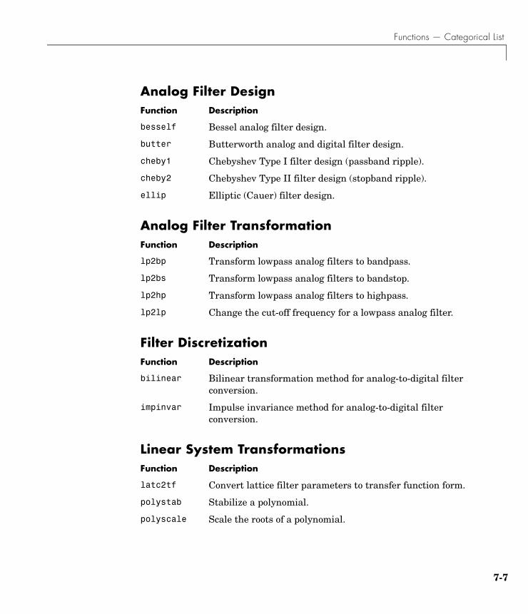
Functions — Categorical List
Analog Filter Design
Analog Filter Transformation
Filter Discretization
Linear System Transformations
Function Description
besself Bessel analog filter design.
butter Butterworth analog and digital filter design.
cheby1 Chebyshev Type I filter design (passband ripple).
cheby2 Chebyshev Type II filter design (stopband ripple).
ellip Elliptic (Cauer) filter design.
Function Description
lp2bp Transform lowpass analog filters to bandpass.
lp2bs Transform lowpass analog filters to bandstop.
lp2hp Transform lowpass analog filters to highpass.
lp2lp Change the cut-off frequency for a lowpass analog filter.
Function Description
bilinear Bilinear transformation method for analog-to-digital filter conversion.
impinvar Impulse invariance method for analog-to-digital filter conversion.
Function Description
latc2tf Convert lattice filter parameters to transfer function form.
polystab Stabilize a polynomial.
polyscale Scale the roots of a polynomial.
7-7
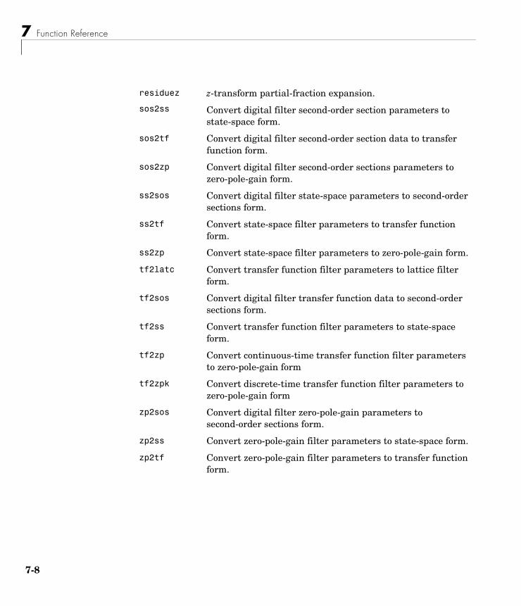
7 Function Reference
7-8
residuez z-transform partial-fraction expansion.
sos2ss Convert digital filter second-order section parameters to state-space form.
sos2tf Convert digital filter second-order section data to transfer function form.
sos2zp Convert digital filter second-order sections parameters to zero-pole-gain form.
ss2sos Convert digital filter state-space parameters to second-order sections form.
ss2tf Convert state-space filter parameters to transfer function form.
ss2zp Convert state-space filter parameters to zero-pole-gain form.
tf2latc Convert transfer function filter parameters to lattice filter form.
tf2sos Convert digital filter transfer function data to second-order sections form.
tf2ss Convert transfer function filter parameters to state-space form.
tf2zp Convert continuous-time transfer function filter parameters to zero-pole-gain form
tf2zpk Convert discrete-time transfer function filter parameters to zero-pole-gain form
zp2sos Convert digital filter zero-pole-gain parameters to second-order sections form.
zp2ss Convert zero-pole-gain filter parameters to state-space form.
zp2tf Convert zero-pole-gain filter parameters to transfer function form.
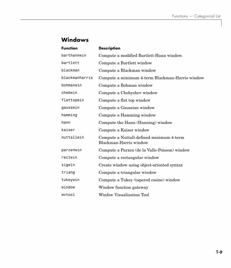
Functions — Categorical List
WindowsFunction Description
barthannwin Compute a modified Bartlett-Hann window.
bartlett Compute a Bartlett window
blackman Compute a Blackman window
blackmanharris Compute a minimum 4-term Blackman-Harris window
bohmanwin Compute a Bohman window
chebwin Compute a Chebyshev window
flattopwin Compute a flat top window
gausswin Compute a Gaussian window
hamming Compute a Hamming window
hann Compute the Hann (Hanning) window
kaiser Compute a Kaiser window
nuttallwin Compute a Nuttall-defined minimum 4-term Blackman-Harris window
parzenwin Compute a Parzen (de la Valle-Poisson) window
rectwin Compute a rectangular window
sigwin Create window using object-oriented syntax
triang Compute a triangular window
tukeywin Compute a Tukey (tapered cosine) window
window Window function gateway
wvtool Winfow Visualization Tool
7-9
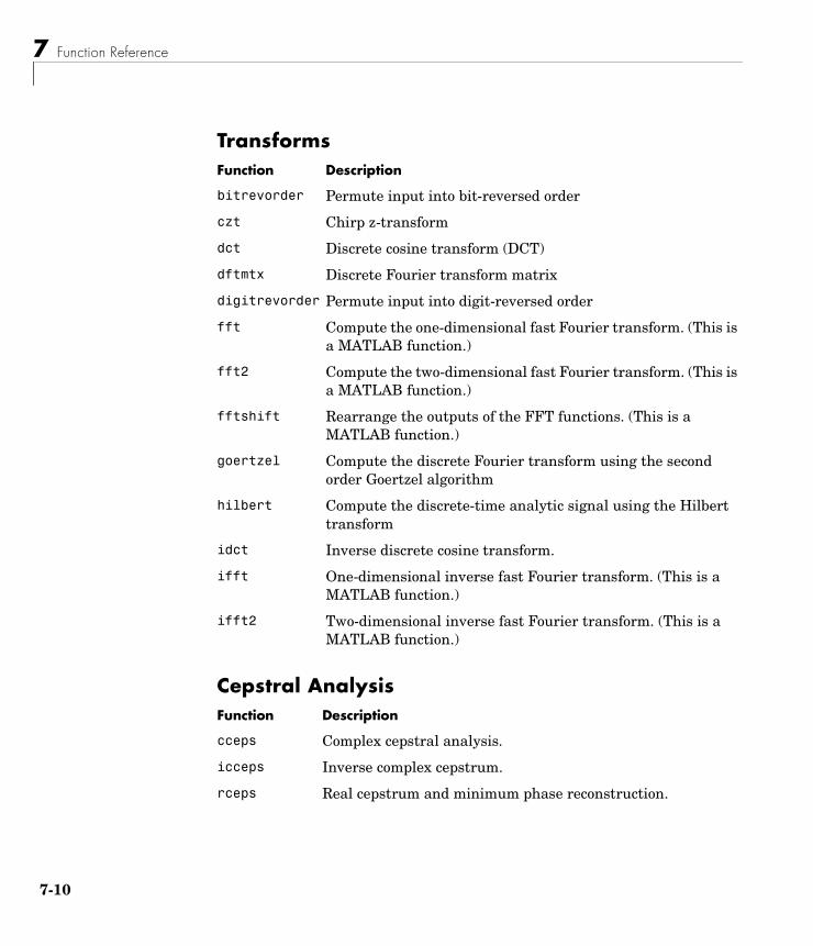
7 Function Reference
7-1
Transforms
Cepstral Analysis
Function Description
bitrevorder Permute input into bit-reversed order
czt Chirp z-transform
dct Discrete cosine transform (DCT)
dftmtx Discrete Fourier transform matrix
digitrevorder Permute input into digit-reversed order
fft Compute the one-dimensional fast Fourier transform. (This is a MATLAB function.)
fft2 Compute the two-dimensional fast Fourier transform. (This is a MATLAB function.)
fftshift Rearrange the outputs of the FFT functions. (This is a MATLAB function.)
goertzel Compute the discrete Fourier transform using the second order Goertzel algorithm
hilbert Compute the discrete-time analytic signal using the Hilbert transform
idct Inverse discrete cosine transform.
ifft One-dimensional inverse fast Fourier transform. (This is a MATLAB function.)
ifft2 Two-dimensional inverse fast Fourier transform. (This is a MATLAB function.)
Function Description
cceps Complex cepstral analysis.
icceps Inverse complex cepstrum.
rceps Real cepstrum and minimum phase reconstruction.
0
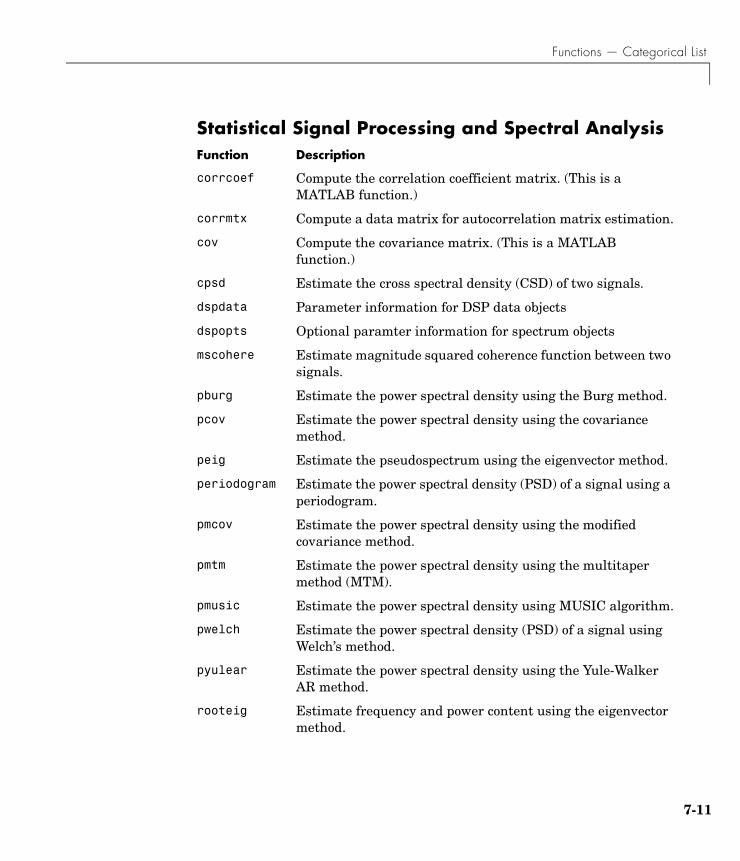
Functions — Categorical List
Statistical Signal Processing and Spectral AnalysisFunction Description
corrcoef Compute the correlation coefficient matrix. (This is a MATLAB function.)
corrmtx Compute a data matrix for autocorrelation matrix estimation.
cov Compute the covariance matrix. (This is a MATLAB function.)
cpsd Estimate the cross spectral density (CSD) of two signals.
dspdata Parameter information for DSP data objects
dspopts Optional paramter information for spectrum objects
mscohere Estimate magnitude squared coherence function between two signals.
pburg Estimate the power spectral density using the Burg method.
pcov Estimate the power spectral density using the covariance method.
peig Estimate the pseudospectrum using the eigenvector method.
periodogram Estimate the power spectral density (PSD) of a signal using a periodogram.
pmcov Estimate the power spectral density using the modified covariance method.
pmtm Estimate the power spectral density using the multitaper method (MTM).
pmusic Estimate the power spectral density using MUSIC algorithm.
pwelch Estimate the power spectral density (PSD) of a signal using Welch’s method.
pyulear Estimate the power spectral density using the Yule-Walker AR method.
rooteig Estimate frequency and power content using the eigenvector method.
7-11
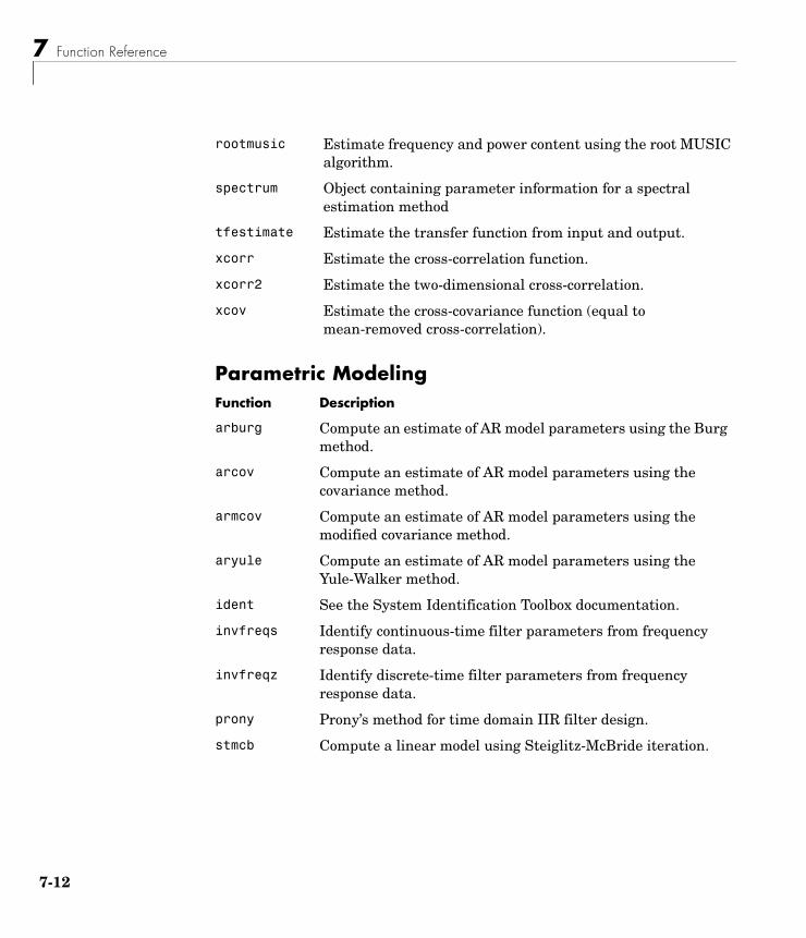
7 Function Reference
7-1
Parametric Modeling
rootmusic Estimate frequency and power content using the root MUSIC algorithm.
spectrum Object containing parameter information for a spectral estimation method
tfestimate Estimate the transfer function from input and output.
xcorr Estimate the cross-correlation function.
xcorr2 Estimate the two-dimensional cross-correlation.
xcov Estimate the cross-covariance function (equal to mean-removed cross-correlation).
Function Description
arburg Compute an estimate of AR model parameters using the Burg method.
arcov Compute an estimate of AR model parameters using the covariance method.
armcov Compute an estimate of AR model parameters using the modified covariance method.
aryule Compute an estimate of AR model parameters using the Yule-Walker method.
ident See the System Identification Toolbox documentation.
invfreqs Identify continuous-time filter parameters from frequency response data.
invfreqz Identify discrete-time filter parameters from frequency response data.
prony Prony’s method for time domain IIR filter design.
stmcb Compute a linear model using Steiglitz-McBride iteration.
2
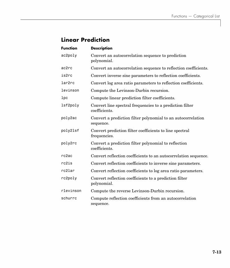
Functions — Categorical List
Linear PredictionFunction Description
ac2poly Convert an autocorrelation sequence to prediction polynomial.
ac2rc Convert an autocorrelation sequence to reflection coefficients.
is2rc Convert inverse sine parameters to reflection coefficients.
lar2rc Convert log area ratio parameters to reflection coefficients.
levinson Compute the Levinson-Durbin recursion.
lpc Compute linear prediction filter coefficients.
lsf2poly Convert line spectral frequencies to a prediction filter coefficients.
poly2ac Convert a prediction filter polynomial to an autocorrelation sequence.
poly2lsf Convert prediction filter coefficients to line spectral frequencies.
poly2rc Convert a prediction filter polynomial to reflection coefficients.
rc2ac Convert reflection coefficients to an autocorrelation sequence.
rc2is Convert reflection coefficients to inverse sine parameters.
rc2lar Convert reflection coefficients to log area ratio parameters.
rc2poly Convert reflection coefficients to a prediction filter polynomial.
rlevinson Compute the reverse Levinson-Durbin recursion.
schurrc Compute reflection coefficients from an autocorrelation sequence.
7-13
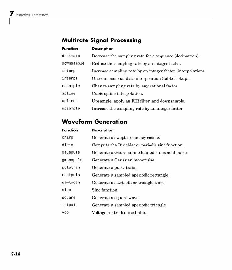
7 Function Reference
7-1
Multirate Signal Processing
Waveform Generation
Function Description
decimate Decrease the sampling rate for a sequence (decimation).
downsample Reduce the sampling rate by an integer factor.
interp Increase sampling rate by an integer factor (interpolation).
interp1 One-dimensional data interpolation (table lookup).
resample Change sampling rate by any rational factor.
spline Cubic spline interpolation.
upfirdn Upsample, apply an FIR filter, and downsample.
upsample Increase the sampling rate by an integer factor
Function Description
chirp Generate a swept-frequency cosine.
diric Compute the Dirichlet or periodic sinc function.
gauspuls Generate a Gaussian-modulated sinusoidal pulse.
gmonopuls Generate a Gaussian monopulse.
pulstran Generate a pulse train.
rectpuls Generate a sampled aperiodic rectangle.
sawtooth Generate a sawtooth or triangle wave.
sinc Sinc function.
square Generate a square wave.
tripuls Generate a sampled aperiodic triangle.
vco Voltage controlled oscillator.
4
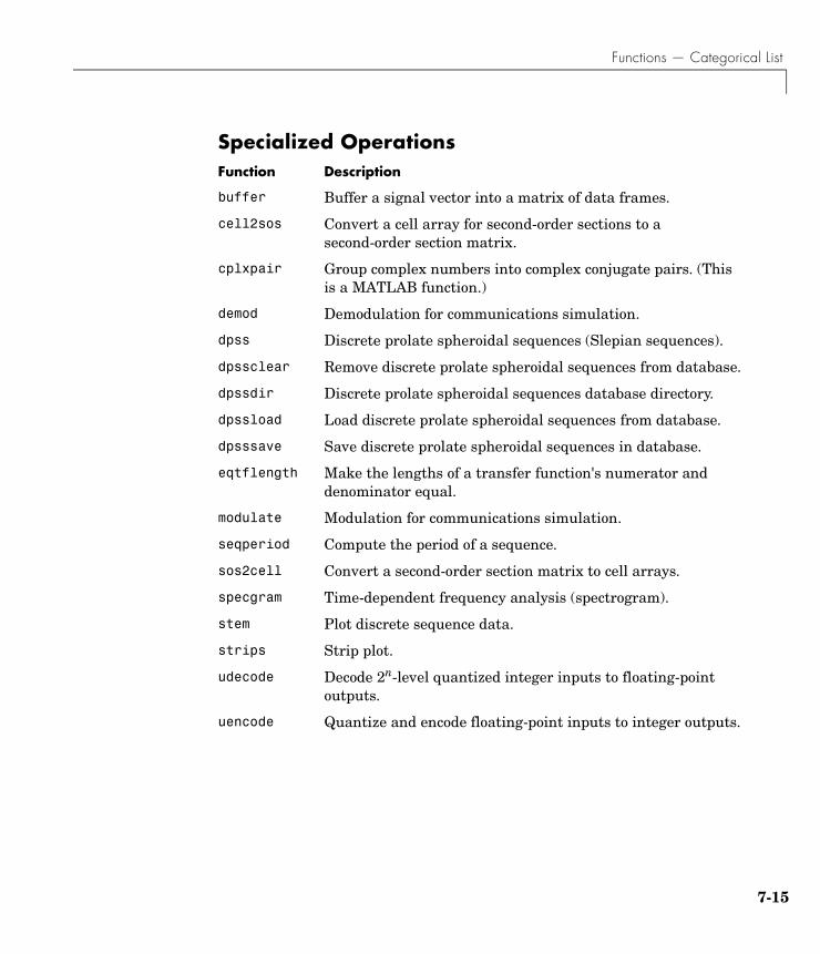
Functions — Categorical List
Specialized OperationsFunction Description
buffer Buffer a signal vector into a matrix of data frames.
cell2sos Convert a cell array for second-order sections to a second-order section matrix.
cplxpair Group complex numbers into complex conjugate pairs. (This is a MATLAB function.)
demod Demodulation for communications simulation.
dpss Discrete prolate spheroidal sequences (Slepian sequences).
dpssclear Remove discrete prolate spheroidal sequences from database.
dpssdir Discrete prolate spheroidal sequences database directory.
dpssload Load discrete prolate spheroidal sequences from database.
dpsssave Save discrete prolate spheroidal sequences in database.
eqtflength Make the lengths of a transfer function's numerator and denominator equal.
modulate Modulation for communications simulation.
seqperiod Compute the period of a sequence.
sos2cell Convert a second-order section matrix to cell arrays.
specgram Time-dependent frequency analysis (spectrogram).
stem Plot discrete sequence data.
strips Strip plot.
udecode Decode 2n-level quantized integer inputs to floating-point outputs.
uencode Quantize and encode floating-point inputs to integer outputs.
7-15
7 Function Reference
7-1
Graphical User InterfacesFunction Description
fdatool Open the Filter Design and Analysis Tool.
fvtool Open the Filter Visualization Tool.
sptool Interactive digital signal processing tool (SPTool).
wintool Open the Window Design and Analysis Tool.
wvtool Open the Window Visualization Tool.
6

Functions — Alphabetical List
Functions — Alphabetical List 7
This section contains function reference pages listed alphabetically.
7-17
abs
7absPurpose Absolute value (magnitude)
abs is a MATLAB function.
Signal-Specific Example
Calculate the magnitude of the FFT of a sequence.
t = (0:99)/100; % Time vectorx = sin(2*pi*15*t) + sin(2*pi*40*t); % Signaly = fft(x); % Compute DFT of xm = abs(y); % Magnitude
Plot the magnitude:
f = (0:length(y)-1)'/length(y)*100; % Frequency vectorplot(f,m)
7-18
ac2poly
7ac2polyPurpose Convert an autocorrelation sequence to a linear prediction filter polynomial
Syntax a = ac2poly(r)[a,efinal] = ac2poly(r)
Description a = ac2poly(r) finds the linear prediction, FIR filter polynomial a corresponding to the autocorrelation sequence r. a is the same length as r, and a(1) = 1. The prediction filter polynomial represents the coefficients of the prediction filter whose output produces a signal whose autocorrelation sequence is approximately the same as the given autocorrelation sequence r.
[a,efinal] = ac2poly(r) returns the final prediction error efinal, determined by running the filter for length(r) steps.
Remarks You can apply this function to real or complex data.
Examples Consider the autocorrelation sequence:
r = [5.0000 -1.5450 -3.9547 3.9331 1.4681 -4.7500];
The corresponding prediction filter polynomial is
[a,efinal] = ac2poly(r)
a = 1.0000 0.6147 0.9898 0.0004 0.0034 -0.0077
efinal =
0.1791
See Also ac2rc, poly2ac, rc2poly
References [1] Kay, S.M. Modern Spectral Estimation. Englewood Cliffs, NJ: Prentice-Hall, 1988.
7-19
ac2rc
7ac2rcPurpose Convert an autocorrelation sequence to reflection coefficients
Syntax [k,r0] = ac2rc(r)
Description [k,r0] = ac2rc(r) finds the reflection coefficients k corresponding to the autocorrelation sequence r. r0 contains the initial zero-lag autocorrelation. These reflection coefficients can be used to specify the lattice prediction filter that produces a sequence with approximately the same autocorrelation sequence as the given sequence r.
Remarks You can apply this function to real or complex data.
See Also ac2poly, poly2rc, rc2ac
References [1] Kay, S.M. Modern Spectral Estimation. Englewood Cliffs, NJ: Prentice-Hall, 1988.
7-20
angle
7anglePurpose Phase angle
angle is a MATLAB function.
Signal-specific Example
Calculate the phase of the FFT of a sequence.
t = (0:99)/100; % Time vectorx = sin(2*pi*15*t) + sin(2*pi*40*t); % Signaly = fft(x); % Compute DFT of xp = unwrap(angle(y)); % Phase
Plot the phase:
f = (0:length(y)-1)'/length(y)*100; % Frequency vectorplot(f,p)
7-21
arburg
7arburgPurpose Compute an estimate of AR model parameters using the Burg method
Syntax a = arburg(x,p)[a,e] = arburg(x,p)[a,e,k] = arburg(x,p)
Description a = arburg(x,p) uses the Burg method to fit a pth order autoregressive (AR) model to the input signal, x, by minimizing (least squares) the forward and backward prediction errors while constraining the AR parameters to satisfy the Levinson-Durbin recursion. x is assumed to be the output of an AR system driven by white noise. Vector a contains the normalized estimate of the AR system parameters, A(z), in descending powers of z.
Since the method characterizes the input data using an all-pole model, the correct choice of the model order p is important.
[a,e] = arburg(x,p) returns the variance estimate, e, of the white noise input to the AR model.
[a,e,k] = arburg(x,p) returns a vector, k, of reflection coefficients.
See Also arcov, armcov, aryule, lpc, pburg, prony
H z( ) eA z( )------------ e
1 a2z 1– … a p 1+( )zp–
+ + +----------------------------------------------------------------------= =
7-22
arcov
7arcovPurpose Compute an estimate of AR model parameters using the covariance method
Syntax a = arcov(x,p)[a,e] = arcov(x,p)
Description a = arcov(x,p) uses the covariance method to fit a pth order autoregressive (AR) model to the input signal, x, which is assumed to be the output of an AR system driven by white noise. This method minimizes the forward prediction error in the least-squares sense. Vector a contains the normalized estimate of the AR system parameters, A(z), in descending powers of z.
Because the method characterizes the input data using an all-pole model, the correct choice of the model order p is important.
[a,e] = arcov(x,p) returns the variance estimate, e, of the white noise input to the AR model.
See Also arburg, armcov, aryule, lpc, pcov, prony
H z( ) eA z( )------------ e
1 a2z 1– … a p 1+( )zp–
+ + +----------------------------------------------------------------------= =
7-23
armcov
7armcovPurpose Compute an estimate of AR model parameters using the modified covariance method
Syntax a = armcov(x,p)[a,e] = armcov(x,p)
Description a = armcov(x,p) uses the modified covariance method to fit a pth order autoregressive (AR) model to the input signal, x, which is assumed to be the output of an AR system driven by white noise. This method minimizes the forward and backward prediction errors in the least-squares sense. Vector a contains the normalized estimate of the AR system parameters, A(z), in descending powers of z.
Because the method characterizes the input data using an all-pole model, the correct choice of the model order p is important.
[a,e] = armcov(x,p) returns the variance estimate, e, of the white noise input to the AR model.
See Also arburg, arcov, aryule, lpc, pmcov, prony
H z( ) eA z( )------------ e
1 a2z 1– … a p 1+( )zp–
+ + +----------------------------------------------------------------------= =
7-24
aryule
7aryulePurpose Compute an estimate of AR model parameters using the Yule-Walker method
Syntax a = aryule(x,p)[a,e] = aryule(x,p)[a,e,k] = aryule(x,p)
Description a = aryule(x,p) uses the Yule-Walker method, also called the autocorrelation method, to fit a pth order autoregressive (AR) model to the windowed input signal, x, by minimizing the forward prediction error in the least-squares sense. This formulation leads to the Yule-Walker equations, which are solved by the Levinson-Durbin recursion. x is assumed to be the output of an AR system driven by white noise. Vector a contains the normalized estimate of the AR system parameters, A(z), in descending powers of z.
Because the method characterizes the input data using an all-pole model, the correct choice of the model order p is important.
[a,e] = aryule(x,p) returns the variance estimate, e, of the white noise input to the AR model.
[a,e,k] = aryule(x,p) returns a vector, k, of reflection coefficients.
See Also arburg, arcov, armcov, lpc, prony, pyulear
H z( ) eA z( )------------ e
1 a2z 1– … a p 1+( )zp–
+ + +----------------------------------------------------------------------= =
7-25
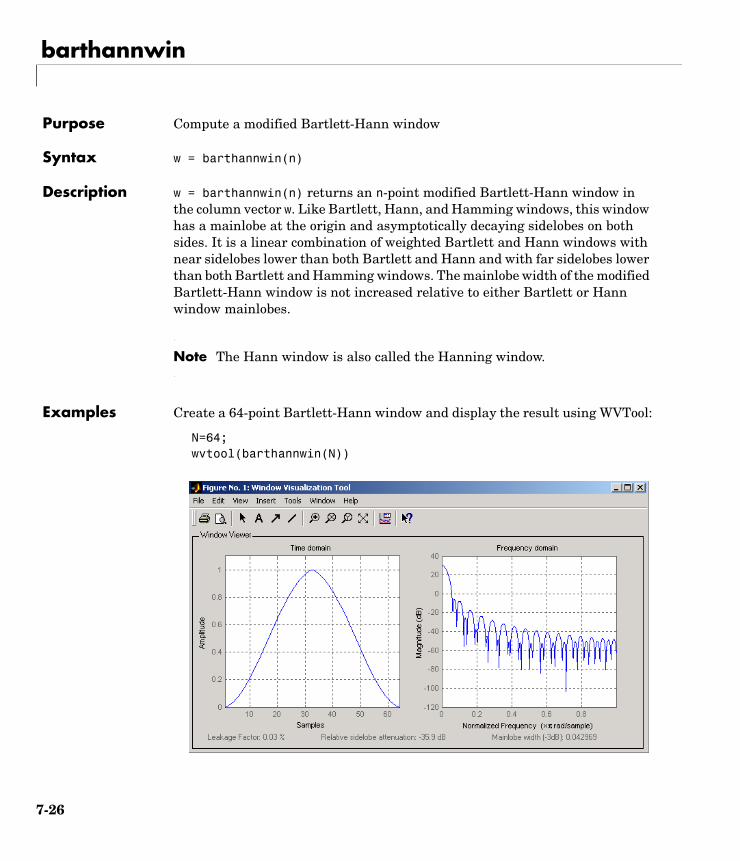
barthannwin
7barthannwinPurpose Compute a modified Bartlett-Hann window
Syntax w = barthannwin(n)
Description w = barthannwin(n) returns an n-point modified Bartlett-Hann window in the column vector w. Like Bartlett, Hann, and Hamming windows, this window has a mainlobe at the origin and asymptotically decaying sidelobes on both sides. It is a linear combination of weighted Bartlett and Hann windows with near sidelobes lower than both Bartlett and Hann and with far sidelobes lower than both Bartlett and Hamming windows. The mainlobe width of the modified Bartlett-Hann window is not increased relative to either Bartlett or Hann window mainlobes.
Note The Hann window is also called the Hanning window.
Examples Create a 64-point Bartlett-Hann window and display the result using WVTool:
N=64;wvtool(barthannwin(N))
7-26
barthannwin
Algorithm The equation for computing the coefficients of a Modified Bartlett-Hanning window is
where .
See Also bartlett, blackmanharris, bohmanwin, nuttallwin, parzenwin, rectwin, triang, window, wintool, wvtool
References [1] Ha, Y.H., and J.A. Pearce. “A New Window and Comparison to Standard Windows.” IEEE Transactions on Acoustics, Speech, and Signal Processing. Vol. 37, No. 2, (February 1999). pp. 298-301.
[2] Oppenheim, A.V., and R.W. Schafer. Discrete-Time Signal Processing. Upper Saddle River, NJ: Prentice-Hall, 1999, p. 468.
w k 1+[ ] 0.62 0.48 kn 1–------------- 0.5– – 0.38 2π k
n 1–------------- 0.5–
cos+=
0 k n 1–( )≤ ≤
7-27
bartlett
7bartlettPurpose Compute a Bartlett window
Syntax w = bartlett(n)
Description w = bartlett(n) returns an n-point Bartlett window in the column vector w, where n must be a positive integer. The coefficients of a Bartlett window are computed as follows:
• For n odd
• For n even
The Bartlett window is very similar to a triangular window as returned by the triang function. The Bartlett window always ends with zeros at samples 1 and n, however, while the triangular window is nonzero at those points. For n odd, the center n-2 points of bartlett(n) are equivalent to triang(n-2).
Note If you specify a one-point window (set n=1), the value 1 is returned.
Examples Create a 64-point Bartlett window and display the result using WVTool:
N=64;wvtool(bartlett(N))
w k 1+[ ]
2kn 1–------------- 0 k n 1–
2-------------≤ ≤,
2 2 k( )n 1–-------------–
n 1–2
------------- k n 1–≤ ≤,
=
w k 1+[ ]
2 k( )n 1–------------- 0 k n
2--- 1–≤ ≤,
2 n k– 1–( )n 1–
------------------------------ n2--- k n 1–≤ ≤,
=
7-28
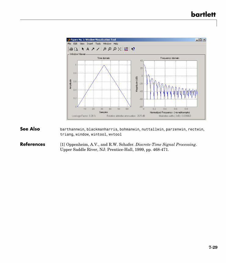
bartlett
See Also barthannwin, blackmanharris, bohmanwin, nuttallwin, parzenwin, rectwin, triang, window, wintool, wvtool
References [1] Oppenheim, A.V., and R.W. Schafer. Discrete-Time Signal Processing. Upper Saddle River, NJ: Prentice-Hall, 1999, pp. 468-471.
7-29
besselap
7besselapPurpose Bessel analog lowpass filter prototype
Syntax [z,p,k] = besselap(n)
Description [z,p,k] = besselap(n) returns the poles and gain of an order n Bessel analog lowpass filter prototype. n must be less than or equal to 25. The function returns the poles in the length n column vector p and the gain in scalar k. z is an empty matrix because there are no zeros. The transfer function is
besselap normalizes the poles and gain so that at low frequency and high frequency the Bessel prototype is asymptotically equivalent to the Butterworth prototype of the same order [1]. The magnitude of the filter is less than at the unity cutoff frequency Ωc = 1.
Analog Bessel filters are characterized by a group delay that is maximally flat at zero frequency and almost constant throughout the passband. The group delay at zero frequency is
Algorithm besselap finds the filter roots from a lookup table constructed using the Symbolic Math Toolbox.
See Also besself, buttap, cheb1ap, cheb2ap, ellipap
Also see the Symbolic Math Toolbox documentation.
References [1] Rabiner, L.R., and B. Gold. Theory and Application of Digital Signal Processing. Englewood Cliffs, NJ: Prentice-Hall, 1975. Pgs. 228-230.
H s( )k
s p 1( )–( ) s p 2( )–( ) s p n( )–( )--------------------------------------------------------------------------------=
1 2⁄
2n( )!2nn!-------------- 1 n⁄
7-30
besself
7besselfPurpose Bessel analog filter design
Syntax [b,a] = besself(n,Wn)[b,a] = besself(n,Wn,'ftype')[z,p,k] = besself(...)[A,B,C,D] = besself(...)
Description besself designs lowpass, bandpass, highpass, and bandstop analog Bessel filters. Analog Bessel filters are characterized by almost constant group delay across the entire passband, thus preserving the wave shape of filtered signals in the passband. Digital Bessel filters do not retain this quality, and besself therefore does not support the design of digital Bessel filters.
[b,a] = besself(n,Wn) designs an order n lowpass analog filter with cutoff frequency Wn. It returns the filter coefficients in the length n+1 row vectors b and a, with coefficients in descending powers of s, derived from this transfer function:
Cutoff frequency is the frequency at which the magnitude response of the filter begins to decrease significantly. For besself, the cutoff frequency Wn must be greater than 0. The magnitude response of a Bessel filter designed by besself is always less than at the cutoff frequency, and it decreases as the order n increases.
If Wn is a two-element vector, Wn = [w1 w2] with w1 < w2, then besself(n,Wn) returns an order 2*n bandpass analog filter with passband w1 < ω < w2.
[b,a] = besself(n,Wn,'ftype') designs a highpass or bandstop filter, where the string 'ftype' is
• 'high' for a highpass analog filter with cutoff frequency Wn
• 'stop' for an order 2*n bandstop analog filter if Wn is a two-element vector, Wn = [w1 w2]. The stopband is w1 < ω < w2.
With different numbers of output arguments, besself directly obtains other realizations of the analog filter. To obtain zero-pole-gain form, use three output arguments as shown below.
H s( )B s( )A s( )----------- b 1( )sn b 2( )sn 1– b n 1+( )+ + +
sn a 2( )sn 1– a n 1+( )+ + +-------------------------------------------------------------------------------------= =
1 2⁄
7-31
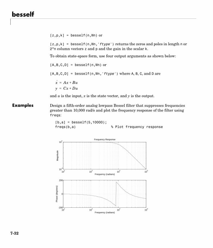
besself
[z,p,k] = besself(n,Wn) or
[z,p,k] = besself(n,Wn,'ftype') returns the zeros and poles in length n or 2*n column vectors z and p and the gain in the scalar k.
To obtain state-space form, use four output arguments as shown below:
[A,B,C,D] = besself(n,Wn) or
[A,B,C,D] = besself(n,Wn,'ftype') where A, B, C, and D are
and u is the input, x is the state vector, and y is the output.
Examples Design a fifth-order analog lowpass Bessel filter that suppresses frequencies greater than 10,000 rad/s and plot the frequency response of the filter using freqs:
[b,a] = besself(5,10000);freqs(b,a) % Plot frequency response
x· Ax Bu+=
y Cx Du+=
102
103
104
105
-200
0
200
Frequency (radians)
Pha
se (
degr
ees)
102
103
104
105
10-5
100
Frequency (radians)
Mag
nitu
de
Frequency Response
7-32
besself
Limitations Lowpass Bessel filters have a monotonically decreasing magnitude response, as do lowpass Butterworth filters. Compared to the Butterworth, Chebyshev, and elliptic filters, the Bessel filter has the slowest rolloff and requires the highest order to meet an attenuation specification.
For high order filters, the state-space form is the most numerically accurate, followed by the zero-pole-gain form. The transfer function coefficient form is the least accurate; numerical problems can arise for filter orders as low as 15.
Algorithm besself performs a four-step algorithm:
1 It finds lowpass analog prototype poles, zeros, and gain using the besselap function.
2 It converts the poles, zeros, and gain into state-space form.
3 It transforms the lowpass filter into a bandpass, highpass, or bandstop filter with desired cutoff frequencies using a state-space transformation.
4 It converts the state-space filter back to transfer function or zero-pole-gain form, as required.
See Also besselap, butter, cheby1, cheby2, ellip
7-33
bilinear
7bilinearPurpose Bilinear transformation method for analog-to-digital filter conversion
Syntax [zd,pd,kd] = bilinear(z,p,k,fs)[zd,pd,kd] = bilinear(z,p,k,fs,fp)[numd,dend] = bilinear(num,den,fs)[numd,dend] = bilinear(num,den,fs,fp)[Ad,Bd,Cd,Dd] = bilinear(A,B,C,D,fs)[Ad,Bd,Cd,Dd] = bilinear(A,B,C,D,fs,fp)
Description The bilinear transformation is a mathematical mapping of variables. In digital filtering, it is a standard method of mapping the s or analog plane into the z or digital plane. It transforms analog filters, designed using classical filter design techniques, into their discrete equivalents.
The bilinear transformation maps the s-plane into the z-plane by
This transformation maps the jΩ axis (from Ω = -∞ to +∞) repeatedly around the unit circle ( , from ω = −π to π) by
bilinear can accept an optional parameter Fp that specifies prewarping. fp, in hertz, indicates a “match” frequency, that is, a frequency for which the frequency responses before and after mapping match exactly. In prewarped mode, the bilinear transformation maps the s-plane into the z-plane with
With the prewarping option, bilinear maps the jΩ axis (from Ω = -∞ to +∞) repeatedly around the unit circle ( , from ω = −π to π) by
H z( ) H s( )s 2fs
z 1–z 1+------------=
=
ejω
ω 2tan 1– Ω2fs-------- =
H z( ) H s( )s
2πfp
πfp
fs
---- tan
------------------------ z 1–( )z 1+( )
-----------------==
ejω
7-34
bilinear
In prewarped mode, bilinear matches the frequency 2πfp (in radians per second) in the s-plane to the normalized frequency 2πfp/fs (in radians per second) in the z-plane.
The bilinear function works with three different linear system representations: zero-pole-gain, transfer function, and state-space form.
Zero-Pole-Gain
[zd,pd,kd] = bilinear(z,p,k,fs) and
[zd,pd,kd] = bilinear(z,p,k,fs,fp) convert the s-domain transfer function specified by z, p, and k to a discrete equivalent. Inputs z and p are column vectors containing the zeros and poles, k is a scalar gain, and fs is the sampling frequency in hertz. bilinear returns the discrete equivalent in column vectors zd and pd and scalar kd. The optional match frequency, fp is in hertz and is used for prewarping.
Transfer Function
[numd,dend] = bilinear(num,den,fs) and
[numd,dend] = bilinear(num,den,fs,fp) convert an s-domain transfer function given by num and den to a discrete equivalent. Row vectors num and den specify the coefficients of the numerator and denominator, respectively, in descending powers of s.
fs is the sampling frequency in hertz. bilinear returns the discrete equivalent in row vectors numd and dend in descending powers of z (ascending powers of z-1). fp is the optional match frequency, in hertz, for prewarping.
ω 2tan 1–Ω π
fpfs----
tan
2πfp-----------------------------
=
num s( )den s( )-------------------- num 1( )sn num n( )s num n 1+( )+ + +
den 1( )sm den m( )s den m 1+( )+ + +-----------------------------------------------------------------------------------------------------------=
7-35

bilinear
State-Space
[Ad,Bd,Cd,Dd] = bilinear(A,B,C,D,fs) and
[Ad,Bd,Cd,Dd] = bilinear(A,B,C,D,fs,fp) convert the continuous-time state-space system in matrices A, B, C, D
to the discrete-time system:
fs is the sampling frequency in hertz. bilinear returns the discrete equivalent in matrices Ad, Bd, Cd, Dd. The optional match frequency, fp is in hertz and is used for prewarping.
Algorithm bilinear uses one of two algorithms depending on the format of the input linear system you supply. One algorithm works on the zero-pole-gain format and the other on the state-space format. For transfer function representations, bilinear converts to state-space form, performs the transformation, and converts the resulting state-space system back to transfer function form.
Zero-Pole-Gain AlgorithmFor a system in zero-pole-gain form, bilinear performs four steps:
1 If fp is present, it prewarps: fp = 2*pi*fp; fs = fp/tan(fp/fs/2)
otherwise, fs = 2*fs.
2 It strips any zeros at ±∞ using z = z(finite(z));
x· Ax Bu+=
y Cx Du+=
x n 1+[ ] Adx n[ ] Bdu n[ ]+=
y n[ ] Cdx n[ ] Ddu n[ ]+=
7-36
bilinear
3 It transforms the zeros, poles, and gain using pd = (1+p/fs)./(1-p/fs); %Do bilinear transformation zd = (1+z/fs)./(1-z/fs); kd = real(k*prod(fs-z)./prod(fs-p));
4 It adds extra zeros at -1 so the resulting system has equivalent numerator and denominator order.
State-Space AlgorithmFor a system in state-space form, bilinear performs two steps:
1 If fp is present, k = 2*pi*fp/tan(pi*fp/fs); else k = 2*fs.
2 It computes Ad, Bd, Cd, and Dd in terms of A, B, C, and D using
bilinear implements these relations using conventional MATLAB statements. The scalar r is arbitrary; bilinear uses to ensure good quantization noise properties in the resulting system.
Diagnostics bilinear requires that the numerator order be no greater than the denominator order. If this is not the case, bilinear displays
Numerator cannot be higher order than denominator.
For bilinear to distinguish between the zero-pole-gain and transfer function linear system formats, the first two input parameters must be vectors with the same orientation in these cases. If this is not the case, bilinear displays
First two arguments must have the same orientation.
See Also impinvar, lp2bp, lp2bs, lp2hp, lp2lp
Ad I 1k--- A+
I 1k--- A–
1–=
Bd2kr
------- I 1k--- A–
1–B=
Cd rC I 1k--- A–
1–=
Dd1k--- C I 1
k--- A–
1–B D+=
r 2 k⁄=
7-37

bilinear
References [1] Parks, T.W., and C.S. Burrus. Digital Filter Design. New York: John Wiley & Sons, 1987. Pgs. 209-213.
[2] Oppenheim, A.V., and R.W. Schafer. Discrete-Time Signal Processing. Upper Saddle River, NJ: Prentice-Hall, 1999, pp. 450-454.
7-38
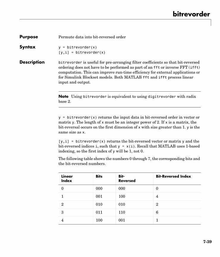
bitrevorder
7bitrevorderPurpose Permute data into bit-reversed order
Syntax y = bitrevorder(x)[y,i] = bitrevorder(x)
Description bitrevorder is useful for pre-arranging filter coefficients so that bit-reversed ordering does not have to be performed as part of an fft or inverse FFT (ifft) computation. This can improve run-time efficiency for external applications or for Simulink Blockset models. Both MATLAB fft and ifft process linear input and output.
Note Using bitrevorder is equivalent to using digitrevorder with radix base 2.
y = bitrevorder(x) returns the input data in bit-reversed order in vector or matrix y. The length of x must be an integer power of 2. If x is a matrix, the bit-reversal occurs on the first dimension of x with size greater than 1. y is the same size as x.
[y,i] = bitrevorder(x) returns the bit-reversed vector or matrix y and the bit-reversed indices i, such that y = x(i). Recall that MATLAB uses 1-based indexing, so the first index of y will be 1, not 0.
The following table shows the numbers 0 through 7, the corresponding bits and the bit-reversed numbers.
Linear Index
Bits Bit-Reversed
Bit-Reversed Index
0 000 000 0
1 001 100 4
2 010 010 2
3 011 110 6
4 100 001 1
7-39
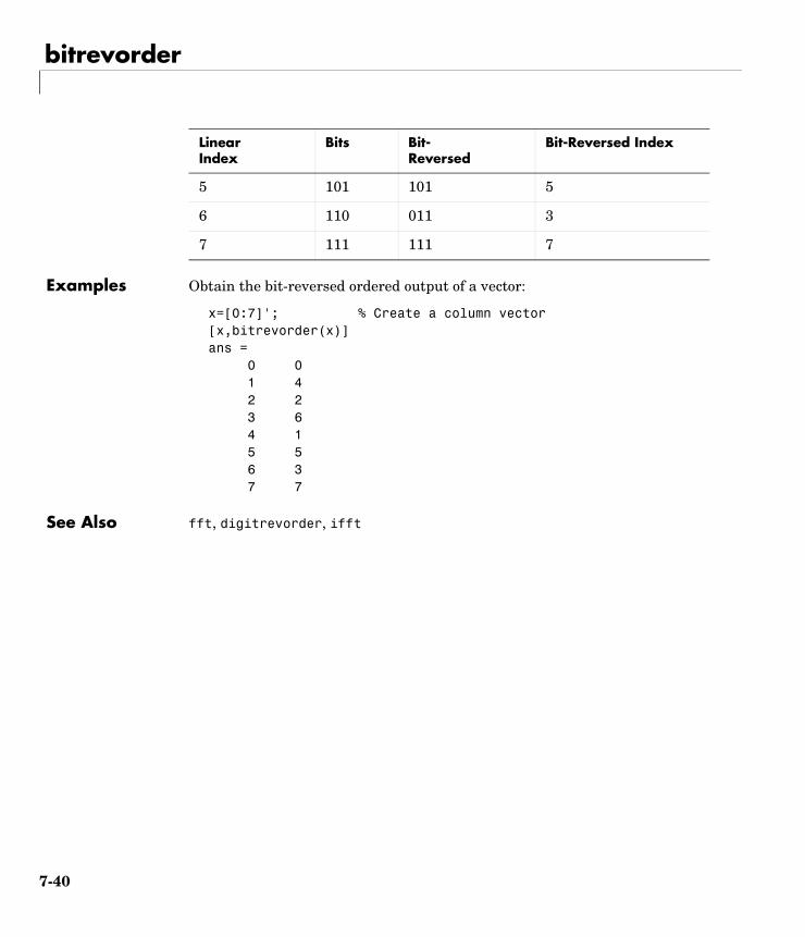
bitrevorder
Examples Obtain the bit-reversed ordered output of a vector:
x=[0:7]'; % Create a column vector[x,bitrevorder(x)]ans = 0 0 1 4 2 2 3 6 4 1 5 5 6 3 7 7
See Also fft, digitrevorder, ifft
5 101 101 5
6 110 011 3
7 111 111 7
Linear Index
Bits Bit-Reversed
Bit-Reversed Index
7-40
blackman
7blackmanPurpose Compute a Blackman window
Syntax w = blackman(n)w = blackman(n,'sflag')
Description w = blackman(n) returns the n-point symmetric Blackman window in the column vector w, where n is a positive integer.
w = blackman(n,'sflag') returns an n-point Blackman window using the window sampling specified by 'sflag', which can be either 'periodic' or 'symmetric' (the default). When 'periodic' is specified, blackman computes a length n+1 window and returns the first n points.
Note If you specify a one-point window (set n=1), the value 1 is returned.
Algorithm The equation for computing the coefficients of a Blackman window is
Blackman windows have slightly wider central lobes and less sideband leakage than equivalent length Hamming and Hann windows.
Examples Create a 64-point Blackman window and display the result using WVTool:
N=64;wvtool(blackman(N))
w k 1+[ ] 0.42 0.5 2π kn 1–-------------
cos– 0.08 4π kn 1–-------------
cos+ k 0= … n 1–, , ,=
7-41
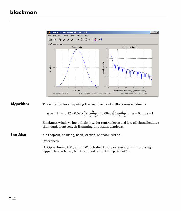
blackman
Algorithm The equation for computing the coefficients of a Blackman window is
Blackman windows have slightly wider central lobes and less sideband leakage than equivalent length Hamming and Hann windows.
See Also flattopwin, hamming, hann, window, wintool, wvtool
References
[1] Oppenheim, A.V., and R.W. Schafer. Discrete-Time Signal Processing. Upper Saddle River, NJ: Prentice-Hall, 1999, pp. 468-471.
w k 1+[ ] 0.42 0.5 2π kn 1–-------------
cos– 0.08 4π kn 1–-------------
cos+ k 0= … n 1–, , ,=
7-42
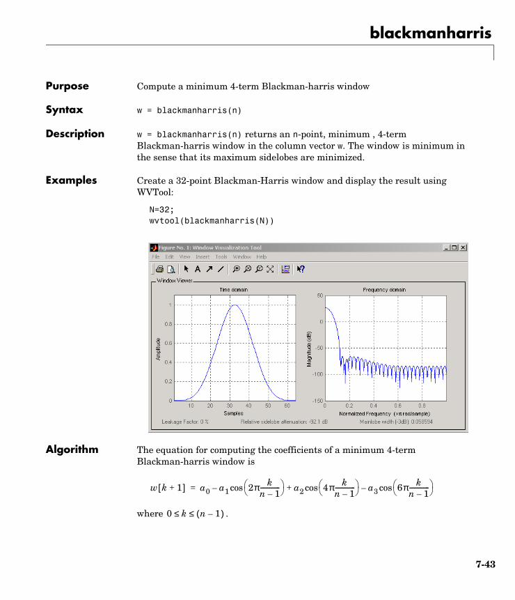
blackmanharris
7blackmanharrisPurpose Compute a minimum 4-term Blackman-harris window
Syntax w = blackmanharris(n)
Description w = blackmanharris(n) returns an n-point, minimum , 4-term Blackman-harris window in the column vector w. The window is minimum in the sense that its maximum sidelobes are minimized.
Examples Create a 32-point Blackman-Harris window and display the result using WVTool:
N=32;wvtool(blackmanharris(N))
Algorithm The equation for computing the coefficients of a minimum 4-term Blackman-harris window is
where .
w k 1+[ ] a0 a1 2π kn 1–-------------
a2 4π kn 1–-------------
cos a3 6π kn 1–-------------
cos–+cos–=
0 k n 1–( )≤ ≤
7-43

blackmanharris
The coefficients for this window are
See Also barthannwin, bartlett, bohmanwin, nuttallwin, parzenwin, rectwin, triang, window, wintool, wvtool
References [1] Harris, F. J. “On the Use of Windows for Harmonic Analysis with the Discrete Fourier Transform.” Proceedings of the IEEE. Vol. 66 (January 1978). pp. 51-84.
a0 = 0.35875
a1 = 0.48829
a2 = 0.14128
a3 = 0.01168
7-44
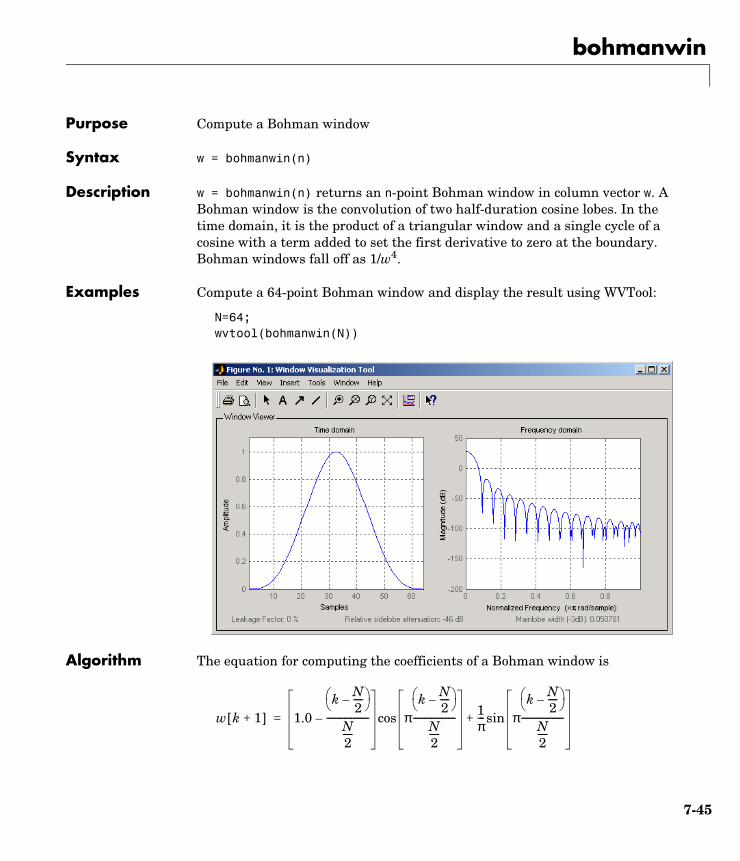
bohmanwin
7bohmanwinPurpose Compute a Bohman window
Syntax w = bohmanwin(n)
Description w = bohmanwin(n) returns an n-point Bohman window in column vector w. A Bohman window is the convolution of two half-duration cosine lobes. In the time domain, it is the product of a triangular window and a single cycle of a cosine with a term added to set the first derivative to zero at the boundary. Bohman windows fall off as 1/w4.
Examples Compute a 64-point Bohman window and display the result using WVTool:
N=64;wvtool(bohmanwin(N))
Algorithm The equation for computing the coefficients of a Bohman window is
w k 1+[ ] 1.0k N
2----–
N2----
-------------------– πk N
2----–
N2----
------------------- 1π--- π
k N2----–
N2----
-------------------sin+cos=
7-45

bohmanwin
where .
See Also barthannwin, bartlett, blackmanharris, nuttallwin, parzenwin, rectwin, triang, window, wintool, wvtool
References [1] Harris, F. J. “On the Use of Windows for Harmonic Analysis with the Discrete Fourier Transform.” Proceedings of the IEEE. Vol. 66 (January 1978). p. 67.
0 k N≤ ≤
7-46
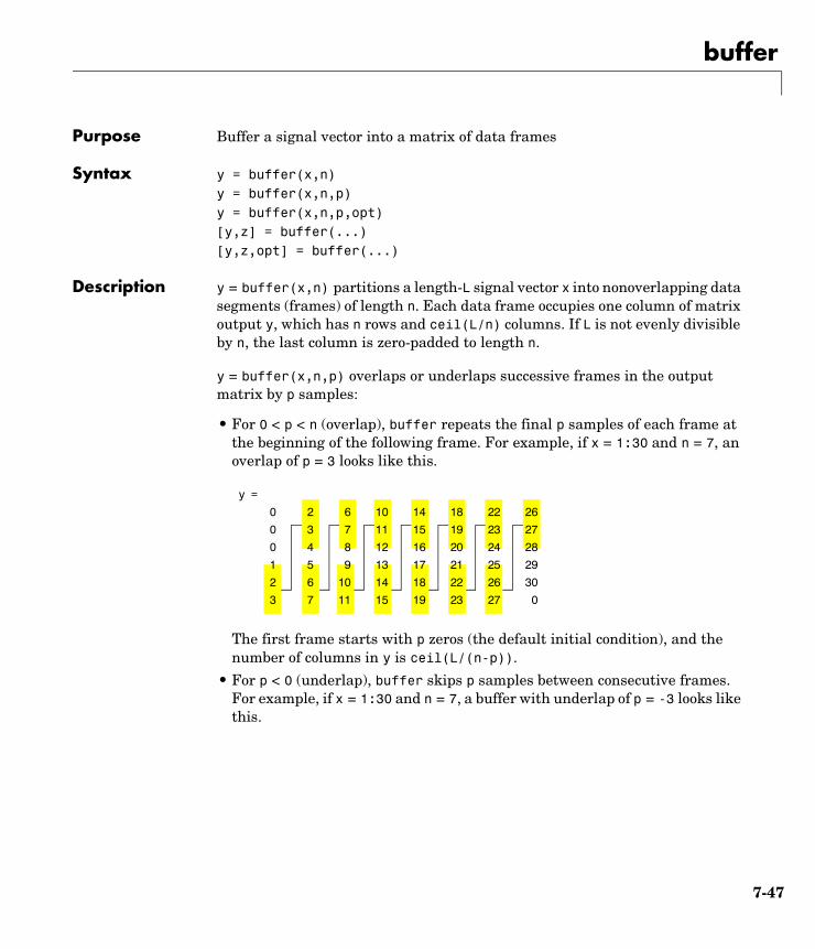
buffer
7bufferPurpose Buffer a signal vector into a matrix of data frames
Syntax y = buffer(x,n)y = buffer(x,n,p)y = buffer(x,n,p,opt)[y,z] = buffer(...)[y,z,opt] = buffer(...)
Description y = buffer(x,n) partitions a length-L signal vector x into nonoverlapping data segments (frames) of length n. Each data frame occupies one column of matrix output y, which has n rows and ceil(L/n) columns. If L is not evenly divisible by n, the last column is zero-padded to length n.
y = buffer(x,n,p) overlaps or underlaps successive frames in the output matrix by p samples:
• For 0 < p < n (overlap), buffer repeats the final p samples of each frame at the beginning of the following frame. For example, if x = 1:30 and n = 7, an overlap of p = 3 looks like this.
The first frame starts with p zeros (the default initial condition), and the number of columns in y is ceil(L/(n-p)).
• For p < 0 (underlap), buffer skips p samples between consecutive frames. For example, if x = 1:30 and n = 7, a buffer with underlap of p = -3 looks like this.
y =
0 2 6 10 14 18 22 26
0 3 7 11 15 19 23 27
0 4 8 12 16 20 24 28
1 5 9 13 17 21 25 29
2 6 10 14 18 22 26 30
3 7 11 15 19 23 27 0
7-47
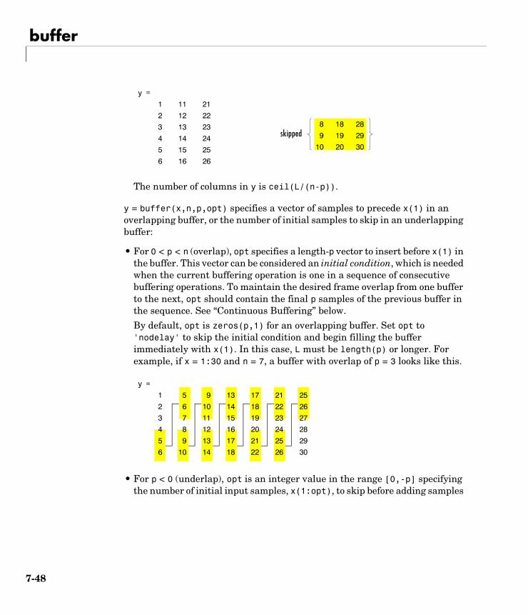
buffer
The number of columns in y is ceil(L/(n-p)).
y = buffer(x,n,p,opt) specifies a vector of samples to precede x(1) in an overlapping buffer, or the number of initial samples to skip in an underlapping buffer:
• For 0 < p < n (overlap), opt specifies a length-p vector to insert before x(1) in the buffer. This vector can be considered an initial condition, which is needed when the current buffering operation is one in a sequence of consecutive buffering operations. To maintain the desired frame overlap from one buffer to the next, opt should contain the final p samples of the previous buffer in the sequence. See “Continuous Buffering” below.
By default, opt is zeros(p,1) for an overlapping buffer. Set opt to 'nodelay' to skip the initial condition and begin filling the buffer immediately with x(1). In this case, L must be length(p) or longer. For example, if x = 1:30 and n = 7, a buffer with overlap of p = 3 looks like this.
• For p < 0 (underlap), opt is an integer value in the range [0,-p] specifying the number of initial input samples, x(1:opt), to skip before adding samples
y =
1 11 21
2 12 22
3 13 23
4 14 24
5 15 25
6 16 26
8 18 28
9 19 29
10 20 30
skipped
y =
1 5 9 13 17 21 25
2 6 10 14 18 22 26
3 7 11 15 19 23 27
4 8 12 16 20 24 28
5 9 13 17 21 25 29
6 10 14 18 22 26 30
7-48
buffer
to the buffer. The first value in the buffer is therefore x(opt+1). By default, opt is zero for an underlapping buffer.
This option is especially useful when the current buffering operation is one in a sequence of consecutive buffering operations. To maintain the desired frame underlap from one buffer to the next, opt should equal the difference between the total number of points to skip between frames (p) and the number of points that were available to be skipped in the previous input to buffer. If the previous input had fewer than p points that could be skipped after filling the final frame of that buffer, the remaining opt points need to be removed from the first frame of the current buffer. See “Continuous Buffering” below for an example of how this works in practice.
[y,z] = buffer(...) partitions the length-L signal vector x into frames of length n, and outputs only the full frames in y. If y is an overlapping buffer, it has n rows and m columns, where
m = floor(L/(n-p)) % When length(opt) = p
or
m = floor((L-n)/(n-p))+1 % When opt = 'nodelay'
If y is an underlapping buffer, it has n rows and m columns, where
m = floor((L-opt)/(n-p)) + (rem((L-opt),(n-p)) >= n)
If the number of samples in the input vector (after the appropriate overlapping or underlapping operations) exceeds the number of places available in the n-by-m buffer, the remaining samples in x are output in vector z, which for an overlapping buffer has length
length(z) = L - m*(n-p) % When length(opt) = p
or
length(z) = L - ((m-1)*(n-p)+n)% When opt = 'nodelay'
and for an underlapping buffer has length
length(z) = (L-opt) - m*(n-p)
7-49

buffer
Output z shares the same orientation (row or column) as x. If there are no remaining samples in the input after the buffer with the specified overlap or underlap is filled, z is an empty vector.
[y,z,opt] = buffer(...) returns the last p samples of a overlapping buffer in output opt. In an underlapping buffer, opt is the difference between the total number of points to skip between frames (-p) and the number of points in x that were available to be skipped after filling the last frame:
• For 0 < p < n (overlap), opt (as an output) contains the final p samples in the last frame of the buffer. This vector can be used as the initial condition for a subsequent buffering operation in a sequence of consecutive buffering operations. This allows the desired frame overlap to be maintained from one buffer to the next. See “Continuous Buffering” below.
• For p < 0 (underlap), opt (as an output) is the difference between the total number of points to skip between frames (-p) and the number of points in x that were available to be skipped after filling the last frame.opt = m*(n-p) + opt - L % z is the empty vector.
where opt on the right-hand side is the input argument to buffer, and opt on the left-hand side is the output argument. Here m is the number of columns in the buffer, which ism = floor((L-opt)/(n-p)) + (rem((L-opt),(n-p))>=n)
Note that for an underlapping buffer output opt is always zero when output z contains data.
The opt output for an underlapping buffer is especially useful when the current buffering operation is one in a sequence of consecutive buffering operations. The opt output from each buffering operation specifies the number of samples that need to be skipped at the start of the next buffering operation to maintain the desired frame underlap from one buffer to the next. If fewer than p points were available to be skipped after filling the final frame of the current buffer, the remaining opt points need to be removed from the first frame of the next buffer.
In a sequence of buffering operations, the opt output from each operation should be used as the opt input to the subsequent buffering operation. This ensures that the desired frame overlap or underlap is maintained from buffer
7-50
buffer
to buffer, as well as from frame to frame within the same buffer. See “Continuous Buffering” below for an example of how this works in practice.
Continuous BufferingIn a continuous buffering operation, the vector input to the buffer function represents one frame in a sequence of frames that make up a discrete signal. These signal frames can originate in a frame-based data acquisition process, or within a frame-based algorithm like the FFT.
As an example, you might acquire data from an A/D card in frames of 64 samples. In the simplest case, you could rebuffer the data into frames of 16 samples; buffer with n = 16 creates a buffer of four frames from each 64-element input frame. The result is that the signal of frame size 64 has been converted to a signal of frame size 16; no samples were added or removed.
In the general case where the original signal frame size, L, is not equally divisible by the new frame size, n, the overflow from the last frame needs to be captured and recycled into the following buffer. You can do this by iteratively calling buffer on input x with the two-output-argument syntax:
[y,z] = buffer([z;x],n) % x is a column vector.
[y,z] = buffer([z,x],n) % x is a row vector.
This simply captures any buffer overflow in z, and prepends the data to the subsequent input in the next call to buffer. Again, the input signal, x, of frame size L, has been converted to a signal of frame size n without any insertion or deletion of samples.
Note that continuous buffering cannot be done with the single-output syntax y = buffer(...), because the last frame of y in this case is zero padded, which adds new samples to the signal.
Continuous buffering in the presence of overlap and underlap is handled with the opt parameter, which is used as both an input and output to buffer. The following two examples demonstrate how the opt parameter should be used.
7-51
buffer
Examples Example 1: Continuous Overlapping BuffersFirst create a buffer containing 100 frames, each with 11 samples:
data = buffer(1:1100,11); % 11 samples per frame
Imagine that the frames (columns) in the matrix called data are the sequential outputs of a data acquisition board sampling a physical signal: data(:,1) is the first D/A output, containing the first 11 signal samples; data(:,2) is the second output, containing the next 11 signal samples, and so on.
You want to rebuffer this signal from the acquired frame size of 11 to a frame size of 4 with an overlap of 1. To do this, you will repeatedly call buffer to operate on each successive input frame, using the opt parameter to maintain consistency in the overlap from one buffer to the next.
Set the buffer parameters:
n = 4; % New frame sizep = 1; % Overlapopt = -5; % Value of y(1)z = []; % Initialize the carry-over vector.
Now repeatedly call buffer, each time passing in a new signal frame from data. Note that overflow samples (returned in z) are carried over and prepended to the input in the subsequent call to buffer:
for i=1:size(data,2), % Loop over each source frame (column). x = data(:,i); % A single frame of the D/A output
[y,z,opt] = buffer([z;x],n,p,opt);
disp(y); % Display the buffer of data.pause
end
7-52
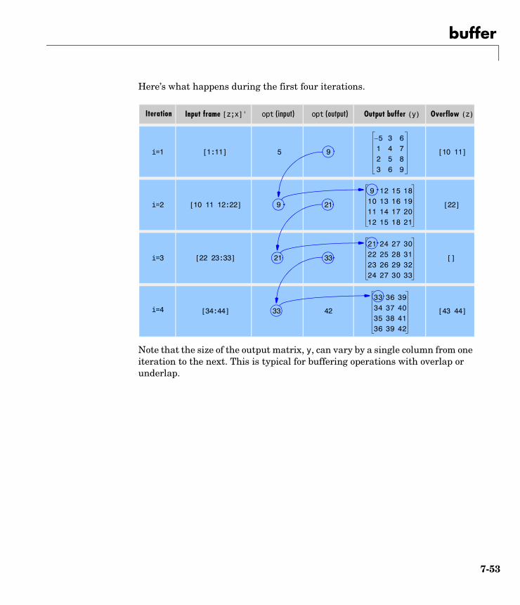
buffer
Here’s what happens during the first four iterations.
Note that the size of the output matrix, y, can vary by a single column from one iteration to the next. This is typical for buffering operations with overlap or underlap.
[1:11]i=1
5– 3 61 4 72 5 83 6 9
Iteration Input frame [z;x]' opt (input) opt (output) Output buffer (y) Overflow (z)
[10 11]5 9
i=2 [10 11 12:22] 9 21
9 12 15 1810 13 16 1911 14 17 2012 15 18 21
[22]
i=3 [22 23:33] 21 33
21 24 27 3022 25 28 3123 26 29 3224 27 30 33
[]
33 36 3934 37 4035 38 4136 39 42
[43 44]42[34:44]i=4 33
7-53
buffer
Example 2: Continuous Underlapping BuffersAgain create a buffer containing 100 frames, each with 11 samples:
data = buffer(1:1100,11); % 11 samples per frame
Again, imagine that data(:,1) is the first D/A output, containing the first 11 signal samples; data(:,2) is the second output, containing the next 11 signal samples, and so on.
You want to rebuffer this signal from the acquired frame size of 11 to a frame size of 4 with an underlap of 2. To do this, you will repeatedly call buffer to operate on each successive input frame, using the opt parameter to maintain consistency in the underlap from one buffer to the next.
Set the buffer parameters:
n = 4; % New frame sizep = -2; % Underlapopt = 1; % Skip the first input element, x(1).z = []; % Initialize the carry-over vector.
Now repeatedly call buffer, each time passing in a new signal frame from data. Note that overflow samples (returned in z) are carried over and prepended to the input in the subsequent call to buffer:
for i=1:size(data,2), % Loop over each source frame (column). x = data(:,i); % A single frame of the D/A output
[y,z,opt] = buffer([z;x],n,p,opt);
disp(y); % Display the buffer of data.pause
end
7-54
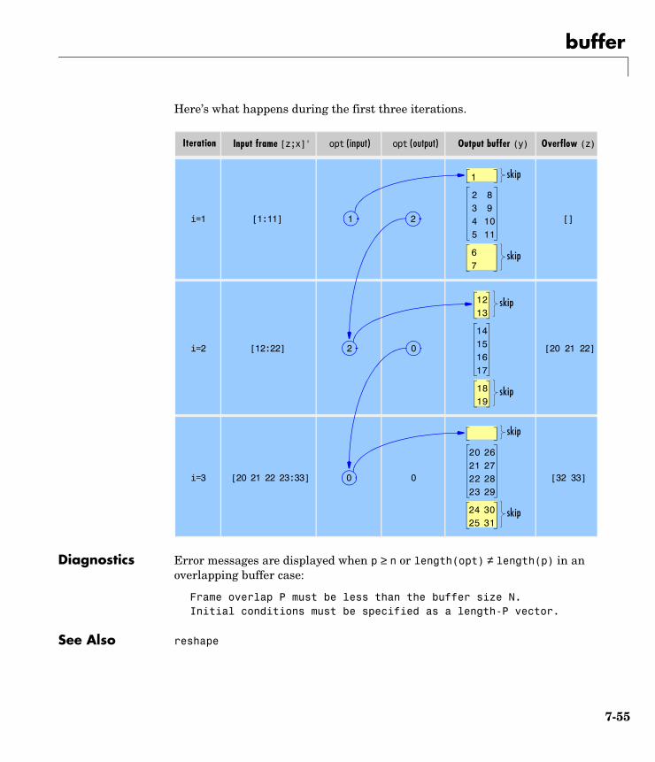
buffer
Here’s what happens during the first three iterations.
Diagnostics Error messages are displayed when p ≥ n or length(opt) ≠ length(p) in an overlapping buffer case:
Frame overlap P must be less than the buffer size N.Initial conditions must be specified as a length-P vector.
See Also reshape
[1:11]i=1
2 83 94 105 11
Iteration Input frame [z;x]' opt (input) opt (output) Output buffer (y) Overflow (z)
[]1 2
i=2 [12:22] 2 0
14151617
[20 21 22]
i=3 [20 21 22 23:33] 0 0
20 2621 2722 2823 29
[32 33]
67
1
1819
1213
24 3025 31
skip
skip
skip
skip
skip
skip
7-55
buttap
7buttapPurpose Butterworth analog lowpass filter prototype
Syntax [z,p,k] = buttap(n)
Description [z,p,k] = buttap(n) returns the poles and gain of an order n Butterworth analog lowpass filter prototype. The function returns the poles in the length n column vector p and the gain in scalar k. z is an empty matrix because there are no zeros. The transfer function is
Butterworth filters are characterized by a magnitude response that is maximally flat in the passband and monotonic overall. In the lowpass case, the first 2n–1 derivatives of the squared magnitude response are zero at ω = 0. The squared magnitude response function is
corresponding to a transfer function with poles equally spaced around a circle in the left half plane. The magnitude response at the cutoff angular frequency ω0 is always regardless of the filter order. buttap sets ω0 to 1 for a normalized result.
Algorithm z = [];p = exp(sqrt(-1)*(pi*(1:2:2*n-1)/(2*n)+pi/2)).';k = real(prod(-p));
See Also besselap, butter, cheb1ap, cheb2ap, ellipap
References [1] Parks, T.W., and C.S. Burrus. Digital Filter Design. New York: John Wiley & Sons, 1987. Chapter 7.
H s( )z s( )p s( )---------- k
s p 1( )–( ) s p 2( )–( ) s p n( )–( )--------------------------------------------------------------------------------= =
H ω( ) 2 11 ω ω0⁄( )2n+------------------------------------=
1 2⁄
7-56
butter
7butterPurpose Butterworth analog and digital filter design
Syntax [b,a] = butter(n,Wn)[b,a] = butter(n,Wn,'ftype')[b,a] = butter(n,Wn,'s')[b,a] = butter(n,Wn,'ftype','s')[z,p,k] = butter(...)[A,B,C,D] = butter(...)
Description butter designs lowpass, bandpass, highpass, and bandstop digital and analog Butterworth filters. Butterworth filters are characterized by a magnitude response that is maximally flat in the passband and monotonic overall.
Butterworth filters sacrifice rolloff steepness for monotonicity in the pass- and stopbands. Unless the smoothness of the Butterworth filter is needed, an elliptic or Chebyshev filter can generally provide steeper rolloff characteristics with a lower filter order.
Digital Domain
[b,a] = butter(n,Wn) designs an order n lowpass digital Butterworth filter with normalized cutoff frequency Wn. It returns the filter coefficients in length n+1 row vectors b and a, with coefficients in descending powers of z.
Cutoff frequency is that frequency where the magnitude response of the filter is . For butter, the normalized cutoff frequency Wn must be a number between 0 and 1, where 1 corresponds to the Nyquist frequency, π radians per sample.
If Wn is a two-element vector, Wn = [w1 w2], butter returns an order 2*n digital bandpass filter with passband w1 < ω < w2.
[b,a] = butter(n,Wn,'ftype') designs a highpass, lowpass, or bandstop filter, where the string 'ftype' is one of the following.
• 'high' for a highpass digital filter with normalized cutoff frequency Wn
• 'low' for a lowpass digital filter with normalized cutoff frequency Wn
H z( )B z( )A z( )----------- b 1( ) b 2( )z 1– b n 1+( )z n–+ + +
1 a 2( )z 1– a n 1+( )z n–+ + +------------------------------------------------------------------------------------= =
1 2⁄
7-57
butter
• 'stop' for an order 2*n bandstop digital filter if Wn is a two-element vector, Wn = [w1 w2]. The stopband is w1 < ω < w2.
With different numbers of output arguments, butter directly obtains other realizations of the filter. To obtain zero-pole-gain form, use three output arguments as shown below:
[z,p,k] = butter(n,Wn) or
[z,p,k] = butter(n,Wn,'ftype') returns the zeros and poles in length n column vectors z and p, and the gain in the scalar k.
To obtain state-space form, use four output arguments as shown below:
[A,B,C,D] = butter(n,Wn) or
[A,B,C,D] = butter(n,Wn,'ftype') where A, B, C, and D are
and u is the input, x is the state vector, and y is the output.
Analog Domain
[b,a] = butter(n,Wn,'s') designs an order n lowpass analog Butterworth filter with angular cutoff frequency Wn rad/s. It returns the filter coefficients in the length n+1 row vectors b and a, in descending powers of s, derived from this transfer function:
butter’s angular cutoff frequency Wn must be greater than 0 rad/s.
If Wn is a two-element vector with w1 < w2, butter(n,Wn,'s') returns an order 2*n bandpass analog filter with passband w1 < ω < w2.
[b,a] = butter(n,Wn,'ftype','s') designs a highpass, lowpass, or bandstop filter.
x n 1+[ ] Ax n[ ] Bu n[ ]+=
y n[ ] Cx n[ ] Du n[ ]+=
H s( )B s( )A s( )----------- b 1( )sn b 2( )sn 1– b n 1+( )+ + +
sn a 2( )sn 1– a n 1+( )+ + +-------------------------------------------------------------------------------------= =
7-58
butter
With different numbers of output arguments, butter directly obtains other realizations of the analog filter. To obtain zero-pole-gain form, use three output arguments as shown below:
[z,p,k] = butter(n,Wn,'s') or
[z,p,k] = butter(n,Wn,'ftype','s') returns the zeros and poles in length n or 2*n column vectors z and p and the gain in the scalar k.
To obtain state-space form, use four output arguments as shown below:
[A,B,C,D] = butter(n,Wn,'s') or
[A,B,C,D] = butter(n,Wn,'ftype','s') where A, B, C, and D are
and u is the input, x is the state vector, and y is the output.
Examples Example 1For data sampled at 1000 Hz, design a 9th-order highpass Butterworth filter with cutoff frequency of 300 Hz, which corresponds to a normalized value of 0.6:
[b,a] = butter(9,300/500,'high');
The filter’s frequency response is
freqz(b,a,128,1000)
x· Ax Bu+=
y Cx Du+=
7-59
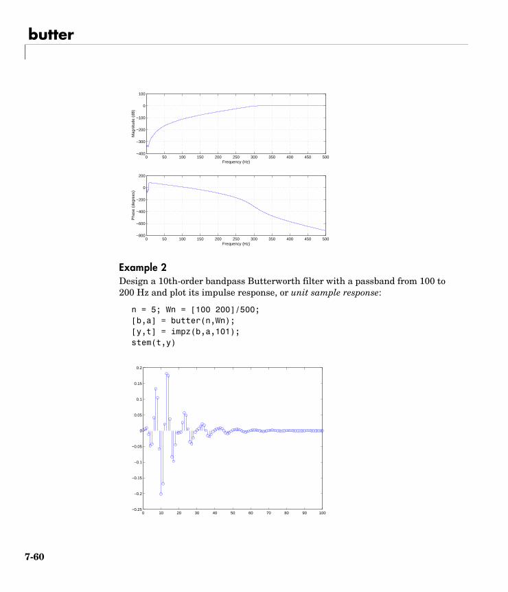
butter
Example 2Design a 10th-order bandpass Butterworth filter with a passband from 100 to 200 Hz and plot its impulse response, or unit sample response:
n = 5; Wn = [100 200]/500;[b,a] = butter(n,Wn);[y,t] = impz(b,a,101);stem(t,y)
0 50 100 150 200 250 300 350 400 450 500−800
−600
−400
−200
0
200
Frequency (Hz)
Pha
se (
degr
ees)
0 50 100 150 200 250 300 350 400 450 500−400
−300
−200
−100
0
100
Frequency (Hz)
Mag
nitu
de (
dB)
0 10 20 30 40 50 60 70 80 90 100−0.25
−0.2
−0.15
−0.1
−0.05
0
0.05
0.1
0.15
0.2
7-60
butter
Limitations For high order filters, the state-space form is the most numerically accurate, followed by the zero-pole-gain form. The transfer function coefficient form is the least accurate; numerical problems can arise for filter orders as low as 15.
Algorithm butter uses a five-step algorithm:
1 It finds the lowpass analog prototype poles, zeros, and gain using the buttap function.
2 It converts the poles, zeros, and gain into state-space form.
3 It transforms the lowpass filter into a bandpass, highpass, or bandstop filter with desired cutoff frequencies, using a state-space transformation.
4 For digital filter design, butter uses bilinear to convert the analog filter into a digital filter through a bilinear transformation with frequency prewarping. Careful frequency adjustment guarantees that the analog filters and the digital filters will have the same frequency response magnitude at Wn or w1 and w2.
5 It converts the state-space filter back to transfer function or zero-pole-gain form, as required.
See Also besself, buttap, buttord, cheby1, cheby2, ellip, maxflat
7-61
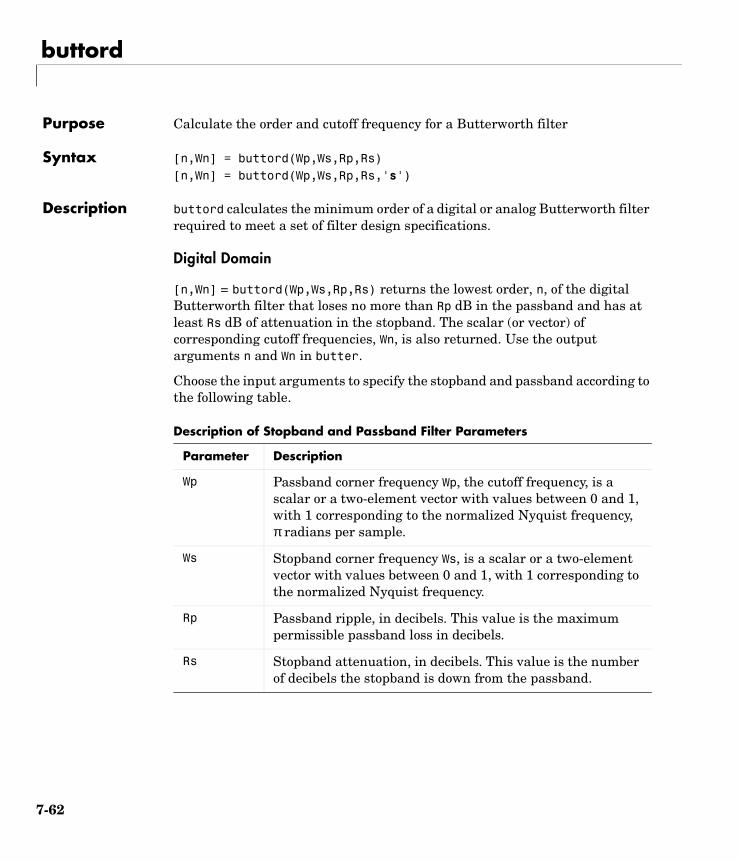
buttord
7buttordPurpose Calculate the order and cutoff frequency for a Butterworth filter
Syntax [n,Wn] = buttord(Wp,Ws,Rp,Rs)[n,Wn] = buttord(Wp,Ws,Rp,Rs,'s')
Description buttord calculates the minimum order of a digital or analog Butterworth filter required to meet a set of filter design specifications.
Digital Domain
[n,Wn] = buttord(Wp,Ws,Rp,Rs) returns the lowest order, n, of the digital Butterworth filter that loses no more than Rp dB in the passband and has at least Rs dB of attenuation in the stopband. The scalar (or vector) of corresponding cutoff frequencies, Wn, is also returned. Use the output arguments n and Wn in butter.
Choose the input arguments to specify the stopband and passband according to the following table.
Description of Stopband and Passband Filter Parameters
Parameter Description
Wp Passband corner frequency Wp, the cutoff frequency, is a scalar or a two-element vector with values between 0 and 1, with 1 corresponding to the normalized Nyquist frequency, π radians per sample.
Ws Stopband corner frequency Ws, is a scalar or a two-element vector with values between 0 and 1, with 1 corresponding to the normalized Nyquist frequency.
Rp Passband ripple, in decibels. This value is the maximum permissible passband loss in decibels.
Rs Stopband attenuation, in decibels. This value is the number of decibels the stopband is down from the passband.
7-62
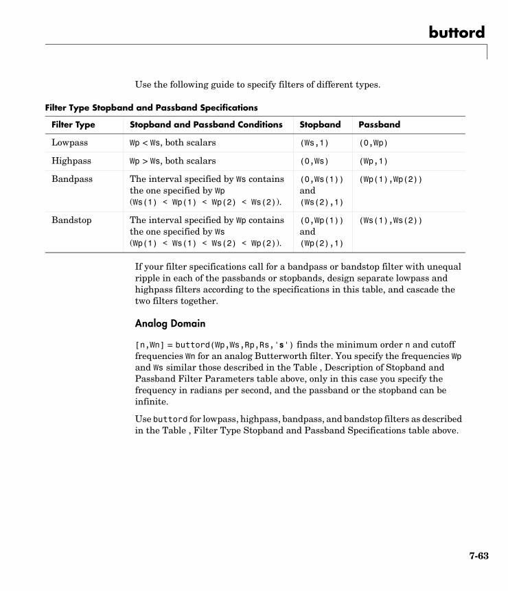
buttord
Use the following guide to specify filters of different types.
If your filter specifications call for a bandpass or bandstop filter with unequal ripple in each of the passbands or stopbands, design separate lowpass and highpass filters according to the specifications in this table, and cascade the two filters together.
Analog Domain
[n,Wn] = buttord(Wp,Ws,Rp,Rs,'s') finds the minimum order n and cutoff frequencies Wn for an analog Butterworth filter. You specify the frequencies Wp and Ws similar those described in the Table , Description of Stopband and Passband Filter Parameters table above, only in this case you specify the frequency in radians per second, and the passband or the stopband can be infinite.
Use buttord for lowpass, highpass, bandpass, and bandstop filters as described in the Table , Filter Type Stopband and Passband Specifications table above.
Filter Type Stopband and Passband Specifications
Filter Type Stopband and Passband Conditions Stopband Passband
Lowpass Wp < Ws, both scalars (Ws,1) (0,Wp)
Highpass Wp > Ws, both scalars (0,Ws) (Wp,1)
Bandpass The interval specified by Ws contains the one specified by Wp (Ws(1) < Wp(1) < Wp(2) < Ws(2)).
(0,Ws(1)) and (Ws(2),1)
(Wp(1),Wp(2))
Bandstop The interval specified by Wp contains the one specified by Ws (Wp(1) < Ws(1) < Ws(2) < Wp(2)).
(0,Wp(1)) and (Wp(2),1)
(Ws(1),Ws(2))
7-63
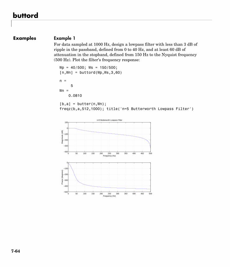
buttord
Examples Example 1For data sampled at 1000 Hz, design a lowpass filter with less than 3 dB of ripple in the passband, defined from 0 to 40 Hz, and at least 60 dB of attenuation in the stopband, defined from 150 Hz to the Nyquist frequency (500 Hz). Plot the filter’s frequency response:
Wp = 40/500; Ws = 150/500;[n,Wn] = buttord(Wp,Ws,3,60)
n = 5Wn = 0.0810
[b,a] = butter(n,Wn);freqz(b,a,512,1000); title('n=5 Butterworth Lowpass Filter')
0 50 100 150 200 250 300 350 400 450 500−500
−400
−300
−200
−100
0
Frequency (Hz)
Ph
ase
(d
eg
ree
s)
0 50 100 150 200 250 300 350 400 450 500−400
−300
−200
−100
0
100
Frequency (Hz)
Ma
gn
itud
e (
dB
)
n=5 Butterworth Lowpass Filter
7-64
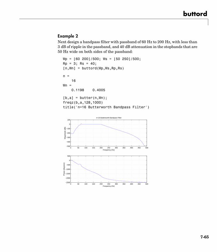
buttord
Example 2Next design a bandpass filter with passband of 60 Hz to 200 Hz, with less than 3 dB of ripple in the passband, and 40 dB attenuation in the stopbands that are 50 Hz wide on both sides of the passband:
Wp = [60 200]/500; Ws = [50 250]/500;Rp = 3; Rs = 40;[n,Wn] = buttord(Wp,Ws,Rp,Rs)
n = 16Wn = 0.1198 0.4005
[b,a] = butter(n,Wn);freqz(b,a,128,1000)title('n=16 Butterworth Bandpass Filter')
0 50 100 150 200 250 300 350 400 450 500−2500
−2000
−1500
−1000
−500
0
500
Frequency (Hz)
Ph
ase
(d
eg
ree
s)
0 50 100 150 200 250 300 350 400 450 500−500
−400
−300
−200
−100
0
100
Frequency (Hz)
Ma
gn
itud
e (
dB
)
n=16 Butterworth Bandpass Filter
7-65
buttord
Algorithm buttord’s order prediction formula is described in [1]. It operates in the analog domain for both analog and digital cases. For the digital case, it converts the frequency parameters to the s-domain before estimating the order and natural frequency, and then converts back to the z-domain.
buttord initially develops a lowpass filter prototype by transforming the passband frequencies of the desired filter to 1 rad/s (for lowpass and highpass filters) and to -1 and 1 rad/s (for bandpass and bandstop filters). It then computes the minimum order required for a lowpass filter to meet the stopband specification.
See Also butter, cheb1ord, cheb2ord, ellipord, kaiserord
References [1] Rabiner, L.R., and B. Gold. Theory and Application of Digital Signal Processing. Englewood Cliffs, NJ: Prentice-Hall, 1975. Pg. 227.
7-66
cceps
7ccepsPurpose Complex cepstral analysis
Syntax xhat = cceps(x)[xhat,nd] = cceps(x)[xhat,nd,xhat1] = cceps(x)[...] = cceps(x,n)
Description Cepstral analysis is a nonlinear signal processing technique that is applied most commonly in speech processing and homomorphic filtering [1].
xhat = cceps(x) returns the complex cepstrum of the (assumed real) sequence x. The input is altered, by the application of a linear phase term, to have no phase discontinuity at ±π radians. That is, it is circularly shifted (after zero padding) by some samples, if necessary, to have zero phase at π radians.
[xhat,nd] = cceps(x) returns the number of samples nd of (circular) delay added to x prior to finding the complex cepstrum.
[xhat,nd,xhat1] = cceps(x) returns a second complex cepstrum, computed using an alternate rooting algorithm, in xhat1. The alternate method ([1] p.795) is useful for short sequences that can be rooted and do not have zeros on the unit circle. For these signals, xhat1 can provide a verification of xhat.
[...] = cceps(x,n) zero pads x to length n and returns the length n complex cepstrum of x.
Algorithm cceps is an M-file implementation of algorithm 7.1 in [2]. A lengthy Fortran program reduces to these three lines of MATLAB code, which compose the core of cceps:
h = fft(x);logh = log(abs(h)) + sqrt(-1)*rcunwrap(angle(h));y = real(ifft(logh));
Note rcunwrap in the above code segment is a special version of unwrap that subtracts a straight line from the phase. rcunwrap is a local function within cceps and is not available for use from the MATLAB command line.
7-67

cceps
See Also icceps, hilbert, rceps, unwrap
References [1] Oppenheim, A.V., and R.W. Schafer. Discrete-Time Signal Processing. Upper Saddle River, NJ: Prentice-Hall, 1999, pp. 788-789.
[2] IEEE. Programs for Digital Signal Processing. IEEE Press. New York: John Wiley & Sons, 1979.
7-68
cell2sos
7cell2sosPurpose Convert a cell array for second-order sections to a second-order section matrix
Syntax m = cell2sos(c)
Description m = cell2sos(c) changes a 1-by-L cell array c consisting of 1-by-2 cell arrays into an L-by-6 second-order section matrix m. Matrix m takes the same form as the matrix generated by tf2sos. You can use m = cell2sos(c) to invert the results of c = sos2cell(m).
c must be a cell array of the form
c = b1 a1 b2 a2 ... bL aL
where both bi and ai are row vectors of at most length 3, and i = 1, 2, ..., L. The resulting matrix m is given by
m = [b1 a1;b2 a2; ... ;bL aL]
See Also sos2cell, tf2sos
7-69
cfirpm
7cfirpmPurpose Complex and nonlinear-phase equiripple FIR filter design
Syntax b = cfirpm(n,f,'fresp')b = cfirpm(n,f,'fresp',w)b = cfirpm(n,f,'fresp',p1,p2,...,w)b = cfirpm(n,f,a,w)b = cfirpm(...,'sym')b = cfirpm(...,'skip_stage2')b = cfirpm(...,'debug')b = cfirpm(...,lgrid)[b,delta,opt] = cfirpm(...)
Description cfirpm allows arbitrary frequency-domain constraints to be specified for the design of a possibly complex FIR filter. The Chebyshev (or minimax) filter error is optimized, producing equiripple FIR filter designs.
b = cfirpm(n,f,'fresp') returns a length n+1 FIR filter with the best approximation to the desired frequency response as returned by function fresp. f is a vector of frequency band edge pairs, specified in the range -1 and 1, where 1 corresponds to the normalized Nyquist frequency. The frequencies must be in increasing order, and f must have even length. The frequency bands span f(k) to f(k+1) for k odd; the intervals f(k+1) to f(k+2) for k odd are “transition bands” or “don’t care” regions during optimization.
b = cfirpm(n,f,'fresp',w) uses the real, non-negative weights in vector w to weight the fit in each frequency band. The length of w is half the length of f, so there is exactly one weight per band.
b = cfirpm(n,f,'fresp',p1,p2,...,...) supplies optional parameters p1, p2, ..., to the frequency response function fresp. Predefined 'fresp' frequency response functions are included for a number of common filter designs, as described below. For all of the predefined frequency response functions, the symmetry option 'sym' defaults to 'even' if no negative frequencies are contained in f and d = 0; otherwise 'sym' defaults to 'none'. (See the 'sym' option below for details.) For all of the predefined frequency response functions, d specifies a group-delay offset such that the filter response has a group delay of n/2+d in units of the sample interval. Negative values create less delay; positive values create more delay. By default d = 0:
7-70
cfirpm
• lowpass, highpass, bandpass, bandstop
These functions share a common syntax, exemplified below by the string 'lowpass'.
b = cfirpm(n,f,'lowpass',...) and
b = cfirpm(n,f,'lowpass',d,...) design a linear-phase (n/2+d delay) filter.
• multiband designs a linear-phase frequency response filter with arbitrary band amplitudes.
b = cfirpm(n,f,'multiband',a,...) and
b = cfirpm(n,f,'multiband',a,d,...) specify vector a containing the desired amplitudes at the band edges in f. The desired amplitude at frequencies between pairs of points f(k) and f(k+1) for k odd is the line segment connecting the points (f(k),a(k)) and (f(k+1),a(k+1)).
• differentiator designs a linear-phase differentiator. For these designs, zero-frequency must be in a transition band, and band weighting is set to be inversely proportional to frequency.
b = cfirpm(n,f,'differentiator',fs,...) and
b = cfirpm(n,f,'differentiator',fs,d,...) specify the sample rate fs used to determine the slope of the differentiator response. If omitted, fs defaults to 1.
• hilbfilt designs a linear-phase Hilbert transform filter response. For Hilbert designs, zero-frequency must be in a transition band.
b = cfirpm(n,f,'hilbfilt',...) and
b = cfirpm(N,F,'hilbfilt',d,...) design a linear-phase (n/2+d delay) Hilbert transform filter.
b = cfirpm(n,f,a,w) is a synonym for b = cfirpm(n,f,'multiband',a,w).
b = cfirpm(...,'sym') imposes a symmetry constraint on the impulse response of the design, where 'sym' may be one of the following:
• 'none' indicates no symmetry constraint. This is the default if any negative band edge frequencies are passed, or if fresp does not supply a default.
• 'even' indicates a real and even impulse response. This is the default for highpass, lowpass, bandpass, bandstop, and multiband designs.
7-71
cfirpm
• 'odd' indicates a real and odd impulse response. This is the default for Hilbert and differentiator designs.
• 'real' indicates conjugate symmetry for the frequency response
If any 'sym' option other than 'none' is specified, the band edges should be specified only over positive frequencies; the negative frequency region is filled in from symmetry. If a 'sym' option is not specified, the fresp function is queried for a default setting. Any user-supplied fresp function should return a valid 'sym'string when it is passed the string 'defaults' as the filter order N.
b = cfirpm(...,'skip_stage2') disables the second-stage optimization algorithm, which executes only when cfirpm determines that an optimal solution has not been reached by the standard firpm error-exchange. Disabling this algorithm may increase the speed of computation, but may incur a reduction in accuracy. By default, the second-stage optimization is enabled.
b = cfirpm(...,'debug') enables the display of intermediate results during the filter design, where 'debug' may be one of 'trace', 'plots', 'both', or 'off'. By default it is set to 'off'.
b = cfirpm(...,lgrid) uses the integer lgrid to control the density of the frequency grid, which has roughly 2^nextpow2(lgrid*n) frequency points. The default value for lgrid is 25. Note that the lgrid argument must be a 1-by-1 cell array.
Any combination of the 'sym', 'skip_stage2', 'debug', and lgrid options may be specified.
[b,delta] = cfirpm(...) returns the maximum ripple height delta.
[b,delta,opt] = cfirpm(...) returns a structure opt of optional results computed by cfirpm and contains the following fields.
Field Description
opt.fgrid Frequency grid vector used for the filter design optimization
opt.des Desired frequency response for each point in opt.fgrid
7-72
cfirpm
User-definable functions may be used, instead of the predefined frequency response functions for fresp. The function is called from within cfirpm using the following syntax
[dh,dw] = fresp(n,f,gf,w,p1,p2,...)
where:
• n is the filter order.
• f is the vector of frequency band edges that appear monotonically between -1 and 1, where 1 corresponds to the Nyquist frequency.
• gf is a vector of grid points that have been linearly interpolated over each specified frequency band by cfirpm. gf determines the frequency grid at which the response function must be evaluated. This is the same data returned by cfirpm in the fgrid field of the opt structure.
• w is a vector of real, positive weights, one per band, used during optimization. w is optional in the call to cfirpm; if not specified, it is set to unity weighting before being passed to fresp.
• dh and dw are the desired complex frequency response and band weight vectors, respectively, evaluated at each frequency in grid gf.
• p1, p2, ..., are optional parameters that may be passed to fresp.
Additionally, a preliminary call is made to fresp to determine the default symmetry property 'sym'. This call is made using the syntax:
sym = fresp('defaults',n,f,[],w,p1,p2,...)
The arguments may be used in determining an appropriate symmetry default as necessary. The function private/lowpass.m may be useful as a template for generating new frequency response functions.
opt.wt Weighting for each point in opt.fgrid
opt.H Actual frequency response for each point in opt.fgrid
opt.error Error at each point in opt.fgrid
opt.iextr Vector of indices into opt.fgrid for extremal frequencies
opt.fextr Vector of extremal frequencies
7-73
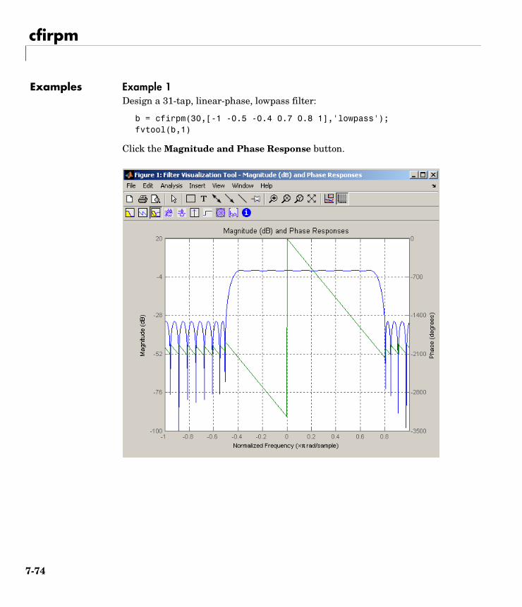
cfirpm
Examples Example 1Design a 31-tap, linear-phase, lowpass filter:
b = cfirpm(30,[-1 -0.5 -0.4 0.7 0.8 1],'lowpass');fvtool(b,1)
Click the Magnitude and Phase Response button.
7-74
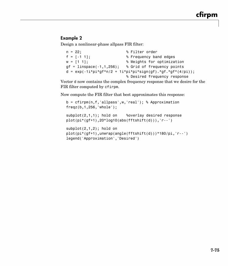
cfirpm
Example 2Design a nonlinear-phase allpass FIR filter:
n = 22; % Filter orderf = [-1 1]; % Frequency band edgesw = [1 1]; % Weights for optimizationgf = linspace(-1,1,256); % Grid of frequency points d = exp(-1i*pi*gf*n/2 + 1i*pi*pi*sign(gf).*gf.*gf*(4/pi));
% Desired frequency responseVector d now contains the complex frequency response that we desire for the FIR filter computed by cfirpm.
Now compute the FIR filter that best approximates this response:
b = cfirpm(n,f,'allpass',w,'real'); % Approximationfreqz(b,1,256,'whole');
subplot(2,1,1); hold on %overlay desired responseplot(pi*(gf+1),20*log10(abs(fftshift(d))),'r--')
subplot(2,1,2); hold onplot(pi*(gf+1),unwrap(angle(fftshift(d)))*180/pi,'r--')legend('Approximation','Desired')
7-75
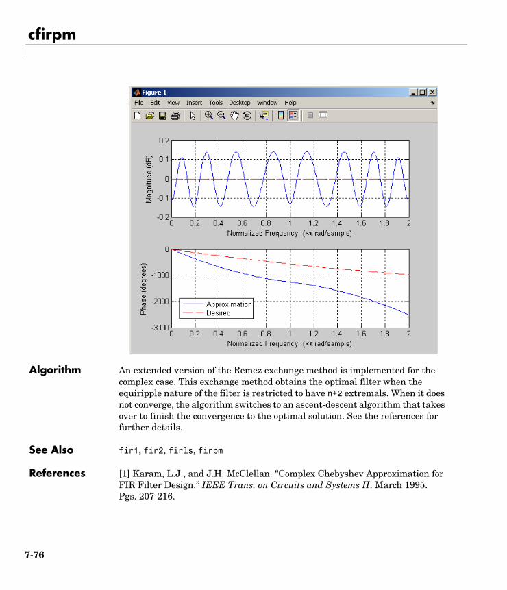
cfirpm
Algorithm An extended version of the Remez exchange method is implemented for the complex case. This exchange method obtains the optimal filter when the equiripple nature of the filter is restricted to have n+2 extremals. When it does not converge, the algorithm switches to an ascent-descent algorithm that takes over to finish the convergence to the optimal solution. See the references for further details.
See Also fir1, fir2, firls, firpm
References [1] Karam, L.J., and J.H. McClellan. “Complex Chebyshev Approximation for FIR Filter Design.” IEEE Trans. on Circuits and Systems II. March 1995. Pgs. 207-216.
7-76
cfirpm
[2] Karam, L.J. Design of Complex Digital FIR Filters in the Chebyshev Sense. Ph.D. Thesis, Georgia Institute of Technology, March 1995.
[3] Demjanjov, V.F., and V.N. Malozemov. Introduction to Minimax. New York: John Wiley & Sons, 1974.
7-77
cheb1ap
7cheb1apPurpose Chebyshev Type I analog lowpass filter prototype
Syntax [z,p,k] = cheb1ap(n,Rp)
Description [z,p,k] = cheb1ap(n,Rp) returns the poles and gain of an order n Chebyshev Type I analog lowpass filter prototype with Rp dB of ripple in the passband. The function returns the poles in the length n column vector p and the gain in scalar k. z is an empty matrix, because there are no zeros. The transfer function is
Chebyshev Type I filters are equiripple in the passband and monotonic in the stopband. The poles are evenly spaced about an ellipse in the left half plane. The Chebyshev Type I cutoff angular frequency is set to 1.0 for a normalized result. This is the frequency at which the passband ends and the filter has magnitude response of 10-Rp/20.
See Also besselap, buttap, cheby1, cheb2ap, ellipap
References [1] Parks, T.W., and C.S. Burrus. Digital Filter Design. New York: John Wiley & Sons, 1987. Chapter 7.
H s( )z s( )p s( )---------- k
s p 1( )–( ) s p 2( )–( ) s p n( )–( )--------------------------------------------------------------------------------= =
ω0
7-78
cheb1ord
7cheb1ordPurpose Calculate the order for a Chebyshev Type I filter
Syntax [n,Wn] = cheb1ord(Wp,Ws,Rp,Rs)[n,Wn] = cheb1ord(Wp,Ws,Rp,Rs,'s')
Description cheb1ord calculates the minimum order of a digital or analog Chebyshev Type I filter required to meet a set of filter design specifications.
Digital Domain
[n,Wn] = cheb1ord(Wp,Ws,Rp,Rs) returns the lowest order n of the Chebyshev Type I filter that loses no more than Rp dB in the passband and has at least Rs dB of attenuation in the stopband. The scalar (or vector) of corresponding cutoff frequencies Wn, is also returned. Use the output arguments n and Wn with the cheby1 function.
Choose the input arguments to specify the stopband and passband according to the following table.
Description of Stopband and Passband Filter Parameters
Parameter Description
Wp Passband corner frequency Wp, the cutoff frequency, is a scalar or a two-element vector with values between 0 and 1, with 1 corresponding to the normalized Nyquist frequency, π radians per sample.
Ws Stopband corner frequency Ws, is a scalar or a two-element vector with values between 0 and 1, with 1 corresponding to the normalized Nyquist frequency.
Rp Passband ripple, in decibels. This value is the maximum permissible passband loss in decibels.
Rs Stopband attenuation, in decibels. This value is the number of decibels the stopband is down from the passband.
7-79
cheb1ord
Use the following guide to specify filters of different types
If your filter specifications call for a bandpass or bandstop filter with unequal ripple in each of the passbands or stopbands, design separate lowpass and highpass filters according to the specifications in this table, and cascade the two filters together.
Analog Domain
[n,Wn] = cheb1ord(Wp,Ws,Rp,Rs,'s') finds the minimum order n and cutoff frequencies Wn for an analog Chebyshev Type I filter. You specify the frequencies Wp and Ws similar to those described in the Table , Description of Stopband and Passband Filter Parameters table above, only in this case you specify the frequency in radians per second, and the passband or the stopband can be infinite.
Use cheb1ord for lowpass, highpass, bandpass, and bandstop filters as described in the Table , Filter Type Stopband and Passband Specifications table above.
Examples For data sampled at 1000 Hz, design a lowpass filter with less than 3 dB of ripple in the passband defined from 0 to 40 Hz and at least 60 dB of ripple in the stopband defined from 150 Hz to the Nyquist frequency (500 Hz):
Wp = 40/500; Ws = 150/500;
Filter Type Stopband and Passband Specifications
Filter Type Stopband and Passband Conditions Stopband Passband
Lowpass Wp < Ws, both scalars (Ws,1) (0,Wp)
Highpass Wp > Ws, both scalars (0,Ws) (Wp,1)
Bandpass The interval specified by Ws contains the one specified by Wp (Ws(1) < Wp(1) < Wp(2) < Ws(2)).
(0,Ws(1)) and (Ws(2),1)
(Wp(1),Wp(2))
Bandstop The interval specified by Wp contains the one specified by Ws (Wp(1) < Ws(1) < Ws(2) < Wp(2)).
(0,Wp(1)) and (Wp(2),1)
(Ws(1),Ws(2))
7-80
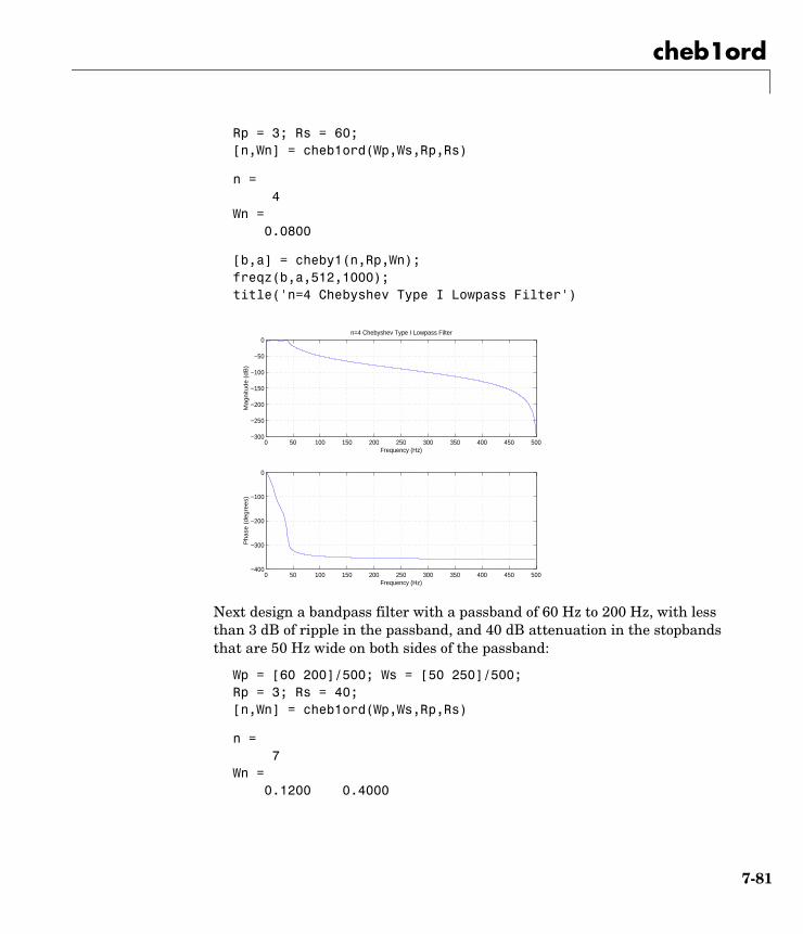
cheb1ord
Rp = 3; Rs = 60;[n,Wn] = cheb1ord(Wp,Ws,Rp,Rs)
n = 4Wn = 0.0800
[b,a] = cheby1(n,Rp,Wn);freqz(b,a,512,1000); title('n=4 Chebyshev Type I Lowpass Filter')
Next design a bandpass filter with a passband of 60 Hz to 200 Hz, with less than 3 dB of ripple in the passband, and 40 dB attenuation in the stopbands that are 50 Hz wide on both sides of the passband:
Wp = [60 200]/500; Ws = [50 250]/500;Rp = 3; Rs = 40;[n,Wn] = cheb1ord(Wp,Ws,Rp,Rs)
n = 7Wn = 0.1200 0.4000
0 50 100 150 200 250 300 350 400 450 500−400
−300
−200
−100
0
Frequency (Hz)
Ph
ase
(d
eg
ree
s)
0 50 100 150 200 250 300 350 400 450 500−300
−250
−200
−150
−100
−50
0
Frequency (Hz)
Ma
gn
itud
e (
dB
)
n=4 Chebyshev Type I Lowpass Filter
7-81
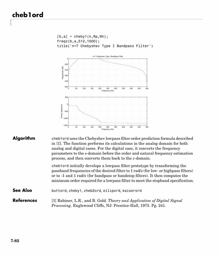
cheb1ord
[b,a] = cheby1(n,Rp,Wn);freqz(b,a,512,1000);title('n=7 Chebyshev Type I Bandpass Filter')
Algorithm cheb1ord uses the Chebyshev lowpass filter order prediction formula described in [1]. The function performs its calculations in the analog domain for both analog and digital cases. For the digital case, it converts the frequency parameters to the s-domain before the order and natural frequency estimation process, and then converts them back to the z-domain.
cheb1ord initially develops a lowpass filter prototype by transforming the passband frequencies of the desired filter to 1 rad/s (for low- or highpass filters) or to -1 and 1 rad/s (for bandpass or bandstop filters). It then computes the minimum order required for a lowpass filter to meet the stopband specification.
See Also buttord, cheby1, cheb2ord, ellipord, kaiserord
References [1] Rabiner, L.R., and B. Gold. Theory and Application of Digital Signal Processing. Englewood Cliffs, NJ: Prentice-Hall, 1975. Pg. 241.
0 50 100 150 200 250 300 350 400 450 500−1500
−1000
−500
0
500
Frequency (Hz)
Ph
ase
(d
eg
ree
s)
0 50 100 150 200 250 300 350 400 450 500−500
−400
−300
−200
−100
0
Frequency (Hz)
Ma
gn
itud
e (
dB
)
n=7 Chebyshev Type I Bandpass Filter
7-82
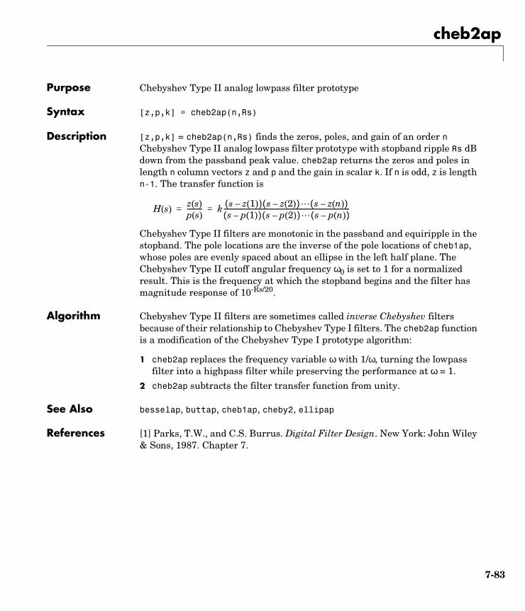
cheb2ap
7cheb2apPurpose Chebyshev Type II analog lowpass filter prototype
Syntax [z,p,k] = cheb2ap(n,Rs)
Description [z,p,k] = cheb2ap(n,Rs) finds the zeros, poles, and gain of an order n Chebyshev Type II analog lowpass filter prototype with stopband ripple Rs dB down from the passband peak value. cheb2ap returns the zeros and poles in length n column vectors z and p and the gain in scalar k. If n is odd, z is length n-1. The transfer function is
Chebyshev Type II filters are monotonic in the passband and equiripple in the stopband. The pole locations are the inverse of the pole locations of cheb1ap, whose poles are evenly spaced about an ellipse in the left half plane. The Chebyshev Type II cutoff angular frequency ω0 is set to 1 for a normalized result. This is the frequency at which the stopband begins and the filter has magnitude response of 10-Rs/20.
Algorithm Chebyshev Type II filters are sometimes called inverse Chebyshev filters because of their relationship to Chebyshev Type I filters. The cheb2ap function is a modification of the Chebyshev Type I prototype algorithm:
1 cheb2ap replaces the frequency variable ω with 1/ω, turning the lowpass filter into a highpass filter while preserving the performance at ω = 1.
2 cheb2ap subtracts the filter transfer function from unity.
See Also besselap, buttap, cheb1ap, cheby2, ellipap
References [1] Parks, T.W., and C.S. Burrus. Digital Filter Design. New York: John Wiley & Sons, 1987. Chapter 7.
H s( )z s( )p s( )---------- k s z 1( )–( ) s z 2( )–( ) s z n( )–( )
s p 1( )–( ) s p 2( )–( ) s p n( )–( )--------------------------------------------------------------------------------= =
7-83
cheb2ord
7cheb2ordPurpose Calculate the order for a Chebyshev Type II filter
Syntax [n,Wn] = cheb2ord(Wp,Ws,Rp,Rs)[n,Wn] = cheb2ord(Wp,Ws,Rp,Rs,'s')
Description cheb2ord calculates the minimum order of a digital or analog Chebyshev Type II filter required to meet a set of filter design specifications.
Digital Domain
[n,Wn] = cheb2ord(Wp,Ws,Rp,Rs) returns the lowest order n of the Chebyshev Type II filter that loses no more than Rp dB in the passband and has at least Rs dB of attenuation in the stopband. The scalar (or vector) of corresponding cutoff frequencies Wn, is also returned. Use the output arguments n and Wn in cheby2.
Choose the input arguments to specify the stopband and passband according to the following table.
Description of Stopband and Passband Filter Parameters
Parameter Description
Wp Passband corner frequency Wp, the cutoff frequency, is a scalar or a two-element vector with values between 0 and 1, with 1 corresponding to the normalized Nyquist frequency, π radians per sample.
Ws Stopband corner frequency Ws, is a scalar or a two-element vector with values between 0 and 1, with 1 corresponding to the normalized Nyquist frequency.
Rp Passband ripple, in decibels. This value is the maximum permissible passband loss in decibels.
Rs Stopband attenuation, in decibels. This value is the number of decibels the stopband is down from the passband.
7-84
cheb2ord
Use the following guide to specify filters of different types.
If your filter specifications call for a bandpass or bandstop filter with unequal ripple in each of the passbands or stopbands, design separate lowpass and highpass filters according to the specifications in this table, and cascade the two filters together.
Analog Domain
[n,Wn] = cheb2ord(Wp,Ws,Rp,Rs,'s') finds the minimum order n and cutoff frequencies Wn for an analog Chebyshev Type II filter. You specify the frequencies Wp and Ws similar to those described in the Table , Description of Stopband and Passband Filter Parameters table above, only in this case you specify the frequency in radians per second, and the passband or the stopband can be infinite.
Use cheb2ord for lowpass, highpass, bandpass, and bandstop filters as described in the Table , Filter Type Stopband and Passband Specifications table above.
Filter Type Stopband and Passband Specifications
Filter Type Stopband and Passband Conditions Stopband Passband
Lowpass Wp < Ws, both scalars (Ws,1) (0,Wp)
Highpass Wp > Ws, both scalars (0,Ws) (Wp,1)
Bandpass The interval specified by Ws contains the one specified by Wp (Ws(1) < Wp(1) < Wp(2) < Ws(2)).
(0,Ws(1)) and (Ws(2),1)
(Wp(1),Wp(2))
Bandstop The interval specified by Wp contains the one specified by Ws (Wp(1) < Ws(1) < Ws(2) < Wp(2)).
(0,Wp(1)) and (Wp(2),1)
(Ws(1),Ws(2))
7-85
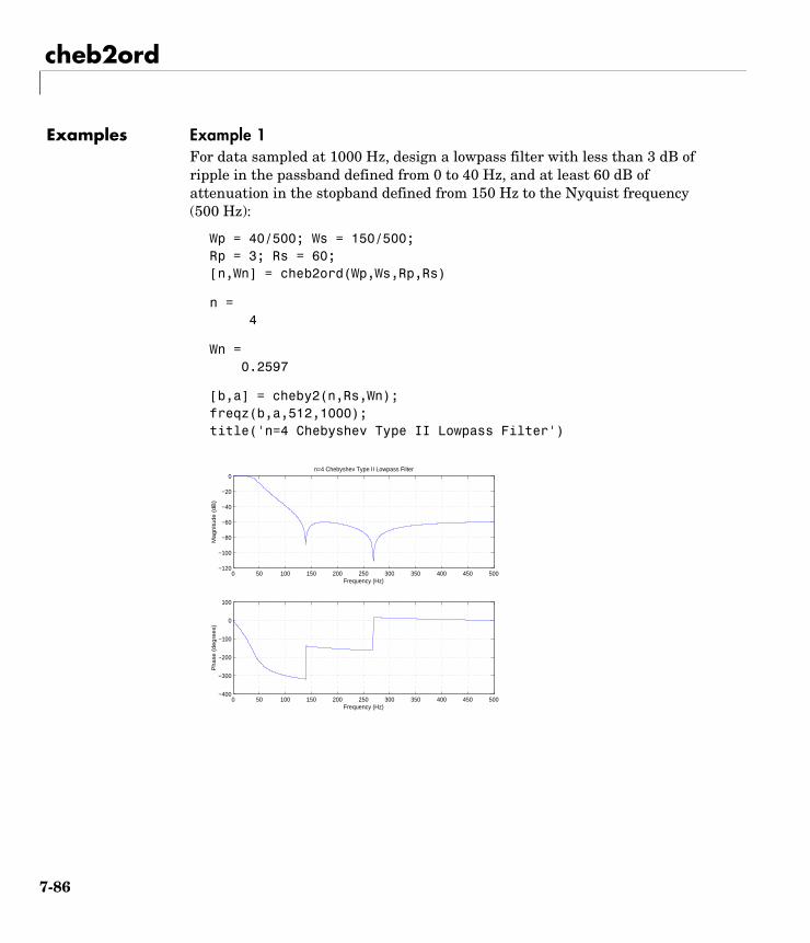
cheb2ord
Examples Example 1For data sampled at 1000 Hz, design a lowpass filter with less than 3 dB of ripple in the passband defined from 0 to 40 Hz, and at least 60 dB of attenuation in the stopband defined from 150 Hz to the Nyquist frequency (500 Hz):
Wp = 40/500; Ws = 150/500;Rp = 3; Rs = 60;[n,Wn] = cheb2ord(Wp,Ws,Rp,Rs)
n = 4
Wn = 0.2597
[b,a] = cheby2(n,Rs,Wn);freqz(b,a,512,1000); title('n=4 Chebyshev Type II Lowpass Filter')
0 50 100 150 200 250 300 350 400 450 500−400
−300
−200
−100
0
100
Frequency (Hz)
Ph
ase
(d
eg
ree
s)
0 50 100 150 200 250 300 350 400 450 500−120
−100
−80
−60
−40
−20
0
Frequency (Hz)
Ma
gn
itud
e (
dB
)
n=4 Chebyshev Type II Lowpass Filter
7-86
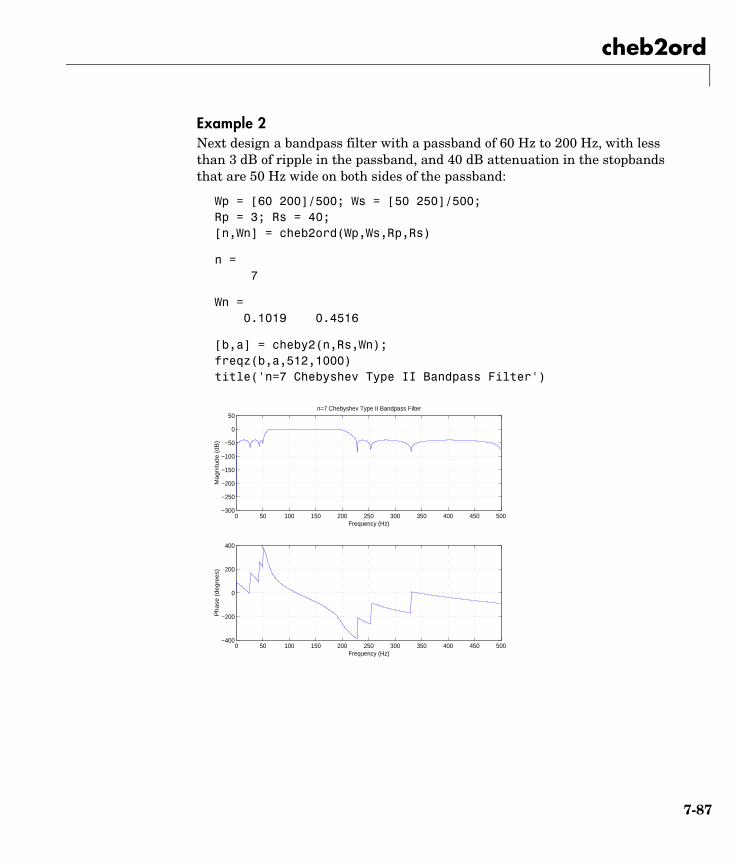
cheb2ord
Example 2Next design a bandpass filter with a passband of 60 Hz to 200 Hz, with less than 3 dB of ripple in the passband, and 40 dB attenuation in the stopbands that are 50 Hz wide on both sides of the passband:
Wp = [60 200]/500; Ws = [50 250]/500;Rp = 3; Rs = 40;[n,Wn] = cheb2ord(Wp,Ws,Rp,Rs)
n = 7
Wn = 0.1019 0.4516
[b,a] = cheby2(n,Rs,Wn);freqz(b,a,512,1000)title('n=7 Chebyshev Type II Bandpass Filter')
0 50 100 150 200 250 300 350 400 450 500−400
−200
0
200
400
Frequency (Hz)
Ph
ase
(d
eg
ree
s)
0 50 100 150 200 250 300 350 400 450 500−300
−250
−200
−150
−100
−50
0
50
Frequency (Hz)
Ma
gn
itud
e (
dB
)
n=7 Chebyshev Type II Bandpass Filter
7-87
cheb2ord
Algorithm cheb2ord uses the Chebyshev lowpass filter order prediction formula described in [1]. The function performs its calculations in the analog domain for both analog and digital cases. For the digital case, it converts the frequency parameters to the s-domain before the order and natural frequency estimation process, and then converts them back to the z-domain.
cheb2ord initially develops a lowpass filter prototype by transforming the stopband frequencies of the desired filter to 1 rad/s (for low- and highpass filters) and to -1 and 1 rad/s (for bandpass and bandstop filters). It then computes the minimum order required for a lowpass filter to meet the passband specification.
See Also buttord, cheb1ord, cheby2, ellipord, kaiserord
References [1] Rabiner, L.R., and B. Gold. Theory and Application of Digital Signal Processing. Englewood Cliffs, NJ: Prentice-Hall, 1975. Pg. 241.
7-88
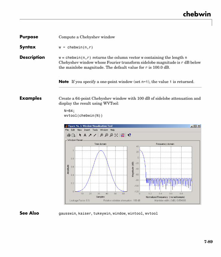
chebwin
7chebwinPurpose Compute a Chebyshev window
Syntax w = chebwin(n,r)
Description w = chebwin(n,r) returns the column vector w containing the length n Chebyshev window whose Fourier transform sidelobe magnitude is r dB below the mainlobe magnitude. The default value for r is 100.0 dB.
Note If you specify a one-point window (set n=1), the value 1 is returned.
Examples Create a 64-point Chebyshev window with 100 dB of sidelobe attenuation and display the result using WVTool:
N=64;wvtool(chebwin(N))
See Also gausswin, kaiser, tukeywin, window, wintool, wvtool
7-89

chebwin
References [1] IEEE. Programs for Digital Signal Processing. IEEE Press. New York: John Wiley & Sons, 1979. Program 5.2.
7-90
cheby1
7cheby1Purpose Chebyshev Type I filter design (passband ripple)
Syntax [b,a] = cheby1(n,Rp,Wn)[b,a] = cheby1(n,Rp,Wn,'ftype')[b,a] = cheby1(n,Rp,Wn,'s')[b,a] = cheby1(n,Rp,Wn,'ftype','s')[z,p,k] = cheby1(...)[A,B,C,D] = cheby1(...)
Description cheby1 designs lowpass, bandpass, highpass, and bandstop digital and analog Chebyshev Type I filters. Chebyshev Type I filters are equiripple in the passband and monotonic in the stopband. Type I filters roll off faster than type II filters, but at the expense of greater deviation from unity in the passband.
Digital Domain
[b,a] = cheby1(n,Rp,Wn) designs an order n Chebyshev lowpass digital Chebyshev filter with normalized cutoff frequency Wn and Rp dB of peak-to-peak ripple in the passband. It returns the filter coefficients in the length n+1 row vectors b and a, with coefficients in descending powers of z.
Normalized cutoff frequency is the frequency at which the magnitude response of the filter is equal to -Rp dB. For cheby1, the normalized cutoff frequency Wn is a number between 0 and 1, where 1 corresponds to the Nyquist frequency, π radians per sample. Smaller values of passband ripple Rp lead to wider transition widths (shallower rolloff characteristics).
If Wn is a two-element vector, Wn = [w1 w2], cheby1 returns an order 2*n bandpass filter with passband w1 < < w2.
[b,a] = cheby1(n,Rp,Wn,'ftype') designs a highpass , lowpass, or bandstop filter, where the string 'ftype' is one of the following
• 'high' for a highpass digital filter with normalized cutoff frequency Wn
• 'low' for a lowpass digital filter with normalized cutoff frequency Wn
H z( )B z( )A z( )----------- b 1( ) b 2( )z 1– b n 1+( )z n–+ + +
1 a 2( )z 1– a n 1+( )z n–+ + +------------------------------------------------------------------------------------= =
ω
7-91
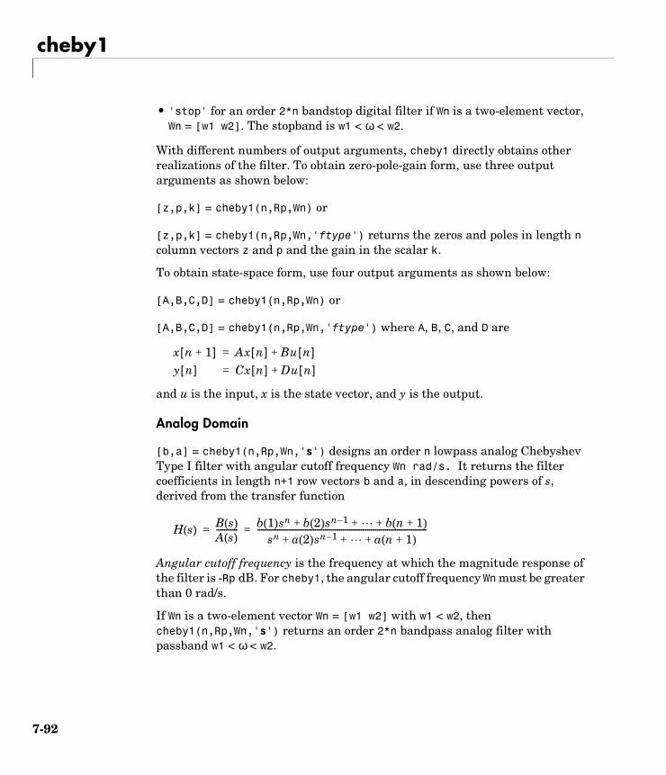
cheby1
• 'stop' for an order 2*n bandstop digital filter if Wn is a two-element vector, Wn = [w1 w2]. The stopband is w1 < ω < w2.
With different numbers of output arguments, cheby1 directly obtains other realizations of the filter. To obtain zero-pole-gain form, use three output arguments as shown below:
[z,p,k] = cheby1(n,Rp,Wn) or
[z,p,k] = cheby1(n,Rp,Wn,'ftype') returns the zeros and poles in length n column vectors z and p and the gain in the scalar k.
To obtain state-space form, use four output arguments as shown below:
[A,B,C,D] = cheby1(n,Rp,Wn) or
[A,B,C,D] = cheby1(n,Rp,Wn,'ftype') where A, B, C, and D are
and u is the input, x is the state vector, and y is the output.
Analog Domain
[b,a] = cheby1(n,Rp,Wn,'s') designs an order n lowpass analog Chebyshev Type I filter with angular cutoff frequency Wn rad/s. It returns the filter coefficients in length n+1 row vectors b and a, in descending powers of s, derived from the transfer function
Angular cutoff frequency is the frequency at which the magnitude response of the filter is -Rp dB. For cheby1, the angular cutoff frequency Wn must be greater than 0 rad/s.
If Wn is a two-element vector Wn = [w1 w2] with w1 < w2, then cheby1(n,Rp,Wn,'s') returns an order 2*n bandpass analog filter with passband w1 < ω < w2.
x n 1+[ ] Ax n[ ] Bu n[ ]+=
y n[ ] Cx n[ ] Du n[ ]+=
H s( )B s( )A s( )----------- b 1( )sn b 2( )sn 1– b n 1+( )+ + +
sn a 2( )sn 1– a n 1+( )+ + +-------------------------------------------------------------------------------------= =
7-92
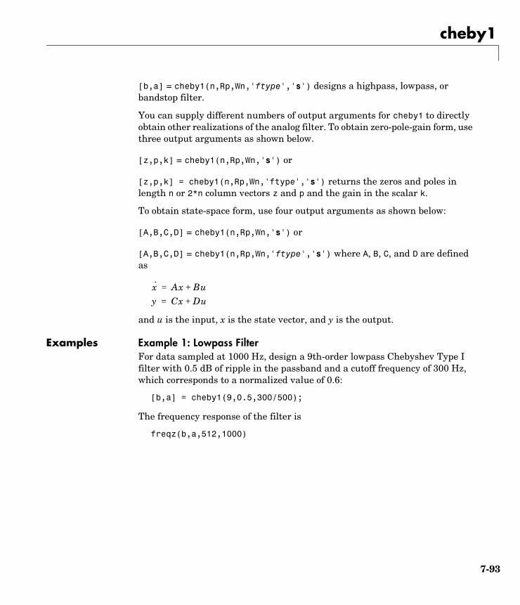
cheby1
[b,a] = cheby1(n,Rp,Wn,'ftype','s') designs a highpass, lowpass, or bandstop filter.
You can supply different numbers of output arguments for cheby1 to directly obtain other realizations of the analog filter. To obtain zero-pole-gain form, use three output arguments as shown below.
[z,p,k] = cheby1(n,Rp,Wn,'s') or
[z,p,k] = cheby1(n,Rp,Wn,'ftype','s') returns the zeros and poles in length n or 2*n column vectors z and p and the gain in the scalar k.
To obtain state-space form, use four output arguments as shown below:
[A,B,C,D] = cheby1(n,Rp,Wn,'s') or
[A,B,C,D] = cheby1(n,Rp,Wn,'ftype','s') where A, B, C, and D are defined as
and u is the input, x is the state vector, and y is the output.
Examples Example 1: Lowpass FilterFor data sampled at 1000 Hz, design a 9th-order lowpass Chebyshev Type I filter with 0.5 dB of ripple in the passband and a cutoff frequency of 300 Hz, which corresponds to a normalized value of 0.6:
[b,a] = cheby1(9,0.5,300/500);
The frequency response of the filter is
freqz(b,a,512,1000)
x· Ax Bu+=
y Cx Du+=
7-93
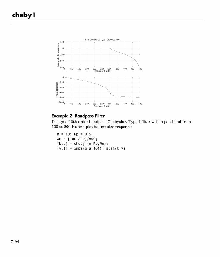
cheby1
Example 2: Bandpass FilterDesign a 10th-order bandpass Chebyshev Type I filter with a passband from 100 to 200 Hz and plot its impulse response:
n = 10; Rp = 0.5;Wn = [100 200]/500;[b,a] = cheby1(n,Rp,Wn);[y,t] = impz(b,a,101); stem(t,y)
0 50 100 150 200 250 300 350 400 450 500-1000
-800
-600
-400
-200
0
Frequency (Hertz)
Pha
se (
degr
ees)
0 50 100 150 200 250 300 350 400 450 500-300
-200
-100
0
100
Frequency (Hertz)
Mag
nitu
de R
espo
nse
(dB
)
n = 9 Chebyshev Type I Lowpass Filter
7-94
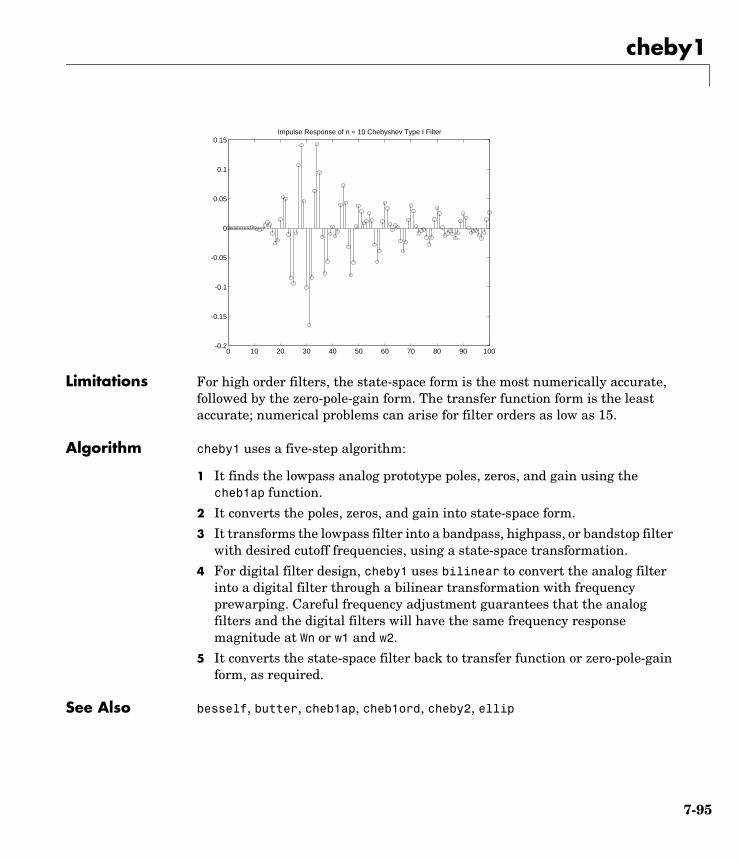
cheby1
Limitations For high order filters, the state-space form is the most numerically accurate, followed by the zero-pole-gain form. The transfer function form is the least accurate; numerical problems can arise for filter orders as low as 15.
Algorithm cheby1 uses a five-step algorithm:
1 It finds the lowpass analog prototype poles, zeros, and gain using the cheb1ap function.
2 It converts the poles, zeros, and gain into state-space form.
3 It transforms the lowpass filter into a bandpass, highpass, or bandstop filter with desired cutoff frequencies, using a state-space transformation.
4 For digital filter design, cheby1 uses bilinear to convert the analog filter into a digital filter through a bilinear transformation with frequency prewarping. Careful frequency adjustment guarantees that the analog filters and the digital filters will have the same frequency response magnitude at Wn or w1 and w2.
5 It converts the state-space filter back to transfer function or zero-pole-gain form, as required.
See Also besself, butter, cheb1ap, cheb1ord, cheby2, ellip
0 10 20 30 40 50 60 70 80 90 100-0.2
-0.15
-0.1
-0.05
0
0.05
0.1
0.15Impulse Response of n = 10 Chebyshev Type I Filter
7-95
cheby2
7cheby2Purpose Chebyshev Type II filter design (stopband ripple)
Syntax [b,a] = cheby2(n,Rs,Wn)[b,a] = cheby2(n,Rs,Wn,'ftype')[b,a] = cheby2(n,Rs,Wn,'s')[b,a] = cheby2(n,Rs,Wn,'ftype','s')[z,p,k] = cheby2(...)[A,B,C,D] = cheby2(...)
Description cheby2 designs lowpass, highpass, bandpass, and bandstop digital and analog Chebyshev Type II filters. Chebyshev Type II filters are monotonic in the passband and equiripple in the stopband. Type II filters do not roll off as fast as type I filters, but are free of passband ripple.
Digital Domain
[b,a] = cheby2(n,Rs,Wn) designs an order n lowpass digital Chebyshev Type II filter with normalized cutoff frequency Wn and stopband ripple Rs dB down from the peak passband value. It returns the filter coefficients in the length n+1 row vectors b and a, with coefficients in descending powers of z.
Normalized cutoff frequency is the beginning of the stopband, where the magnitude response of the filter is equal to -Rs dB. For cheby2, the normalized cutoff frequency Wn is a number between 0 and 1, where 1 corresponds to the Nyquist frequency. Larger values of stopband attenuation Rs lead to wider transition widths (shallower rolloff characteristics).
If Wn is a two-element vector, Wn = [w1 w2], cheby2 returns an order 2*n bandpass filter with passband w1 < ω< w2.
[b,a] = cheby2(n,Rs,Wn,'ftype') designs a highpass, lowpass, or bandstop filter, where the string 'ftype' is one of the following.
• 'high' for a highpass digital filter with normalized cutoff frequency Wn
• 'low' for a lowpass digital filter with normalized cutoff frequency Wn
H z( )B z( )A z( )----------- b 1( ) b 2( )z 1– b n 1+( )z n–+ + +
1 a 2( )z 1– a n 1+( )z n–+ + +------------------------------------------------------------------------------------= =
7-96
cheby2
• 'stop' for an order 2*n bandstop digital filter if Wn is a two-element vector, Wn = [w1 w2]. The stopband is w1 < ω < w2.
With different numbers of output arguments, cheby2 directly obtains other realizations of the filter. To obtain zero-pole-gain form, use three output arguments as shown below:
[z,p,k] = cheby2(n,Rs,Wn) or
[z,p,k] = cheby2(n,Rs,Wn,'ftype') returns the zeros and poles in length n column vectors z and p and the gain in the scalar k.
To obtain state-space form, use four output arguments as shown below.
[A,B,C,D] = cheby2(n,Rs,Wn) or
[A,B,C,D] = cheby2(n,Rs,Wn,'ftype') where A, B, C, and D are
and u is the input, x is the state vector, and y is the output.
Analog Domain
[b,a] = cheby2(n,Rs,Wn,'s') designs an order n lowpass analog Chebyshev Type II filter with angular cutoff frequency Wn. It returns the filter coefficients in the length n+1 row vectors b and a, with coefficients in descending powers of s, derived from the transfer function.
Angular cutoff frequency is the frequency at which the magnitude response of the filter is equal to -Rs dB. For cheby2, the angular cutoff frequency Wn must be greater than 0 rad/s.
If Wn is a two-element vector Wn = [w1 w2] with w1 < w2, then cheby2(n,Rs,Wn,'s') returns an order 2*n bandpass analog filter with passband w1 < ω < w2.
x n 1+[ ] Ax n[ ] Bu n[ ]+=
y n[ ] Cx n[ ] Du n[ ]+=
H s( )B s( )A s( )----------- b 1( )sn b 2( )sn 1– b n 1+( )+ + +
sn a 2( )sn 1– a n 1+( )+ + +-------------------------------------------------------------------------------------= =
7-97
cheby2
[b,a] = cheby2(n,Rs,Wn,'ftype','s') designs a highpass , lowpass, or bandstop filter.
With different numbers of output arguments, cheby2 directly obtains other realizations of the analog filter. To obtain zero-pole-gain form, use three output arguments as shown below:
[z,p,k] = cheby2(n,Rs,Wn,'s') or
[z,p,k] = cheby2(n,Rs,Wn,'ftype','s') returns the zeros and poles in length n or 2*n column vectors z and p and the gain in the scalar k.
To obtain state-space form, use four output arguments as shown below:
[A,B,C,D] = cheby2(n,Rs,Wn,'s') or
[A,B,C,D] = cheby2(n,Rs,Wn,'ftype','s') where A, B, C, and D are
and u is the input, x is the state vector, and y is the output.
Examples Example 1: Lowpass FilterFor data sampled at 1000 Hz, design a ninth-order lowpass Chebyshev Type II filter with stopband attenuation 20 dB down from the passband and a cutoff frequency of 300 Hz, which corresponds to a normalized value of 0.6:
[b,a] = cheby2(9,20,300/500);
The frequency response of the filter is
freqz(b,a,512,1000)
x· Ax Bu+=
y Cx Du+=
7-98
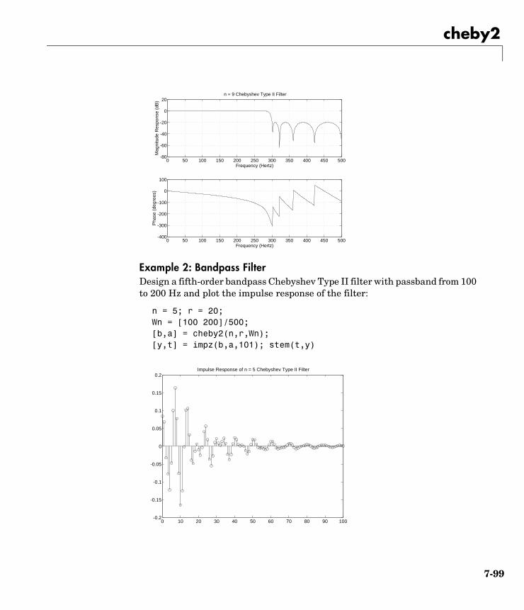
cheby2
Example 2: Bandpass FilterDesign a fifth-order bandpass Chebyshev Type II filter with passband from 100 to 200 Hz and plot the impulse response of the filter:
n = 5; r = 20;Wn = [100 200]/500;[b,a] = cheby2(n,r,Wn);[y,t] = impz(b,a,101); stem(t,y)
0 50 100 150 200 250 300 350 400 450 500-400
-300
-200
-100
0
100
Frequency (Hertz)
Pha
se (
degr
ees)
0 50 100 150 200 250 300 350 400 450 500-80
-60
-40
-20
0
20
Frequency (Hertz)
Mag
nitu
de R
espo
nse
(dB
)
n = 9 Chebyshev Type II Filter
0 10 20 30 40 50 60 70 80 90 100-0.2
-0.15
-0.1
-0.05
0
0.05
0.1
0.15
0.2Impulse Response of n = 5 Chebyshev Type II Filter
7-99
cheby2
Limitations For high order filters, the state-space form is the most numerically accurate, followed by the zero-pole-gain form. The transfer function coefficient form is the least accurate; numerical problems can arise for filter orders as low as 15.
Algorithm cheby2 uses a five-step algorithm:
1 It finds the lowpass analog prototype poles, zeros, and gain using the cheb2ap function.
2 It converts poles, zeros, and gain into state-space form.
3 It transforms the lowpass filter into a bandpass, highpass, or bandstop filter with desired cutoff frequencies, using a state-space transformation.
4 For digital filter design, cheby2 uses bilinear to convert the analog filter into a digital filter through a bilinear transformation with frequency prewarping. Careful frequency adjustment guarantees that the analog filters and the digital filters will have the same frequency response magnitude at Wn or w1 and w2.
5 It converts the state-space filter back to transfer function or zero-pole-gain form, as required.
See Also besself, butter, cheb2ap, cheb1ord, cheby1, ellip
7-100
chirp
7chirpPurpose Generate a swept-frequency cosine
Syntax y = chirp(t,f0,t1,f1)y = chirp(t,f0,t1,f1,'method')y = chirp(t,f0,t1,f1,'method',phi)y = chirp(t,f0,t1,f1,'quadratic',phi,'shape')
Description y = chirp(t,f0,t1,f1) generates samples of a linear swept-frequency cosine signal at the time instances defined in array t, where f0 is the instantaneous frequency at time 0, and f1 is the instantaneous frequency at time t1. f0 and f1 are both in hertz. If unspecified, f0 is 0, t1 is 1, and f1 is 100.
y = chirp(t,f0,t1,f1,'method') specifies alternative sweep method options, where method can be:
• linear, which specifies an instantaneous frequency sweep fi(t) given by
where
β ensures that the desired frequency breakpoint f1 at time t1 is maintained.
• quadratic, which specifies an instantaneous frequency sweep fi(t) given by
where
If f0 > f1 (downsweep), the default shape is convex. If f0 < f1 (upsweep), the default shape is concave.
• logarithmic specifies an instantaneous frequency sweep fi(t) given by
where
fi t( ) f0 βt+=
β f1 f0–( ) t1⁄=
fi t( ) f0 βt2+=
β f1 f0–( ) t12⁄=
fi t( ) f0 10βt+=
7-101
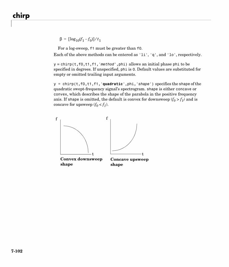
chirp
For a log-sweep, f1 must be greater than f0.
Each of the above methods can be entered as 'li', 'q', and 'lo', respectively.
y = chirp(t,f0,t1,f1,'method',phi) allows an initial phase phi to be specified in degrees. If unspecified, phi is 0. Default values are substituted for empty or omitted trailing input arguments.
y = chirp(t,f0,t1,f1,'quadratic',phi,'shape') specifies the shape of the quadratic swept-frequency signal’s spectrogram. shape is either concave or convex, which describes the shape of the parabola in the positive frequency axis. If shape is omitted, the default is convex for downsweep (f0 > f1) and is concave for upsweep (f0 < f1).
β log10 f1 f0–( )[ ] t1⁄=
Convex downsweep shape
Concave upsweep shape
t
f f
t
7-102
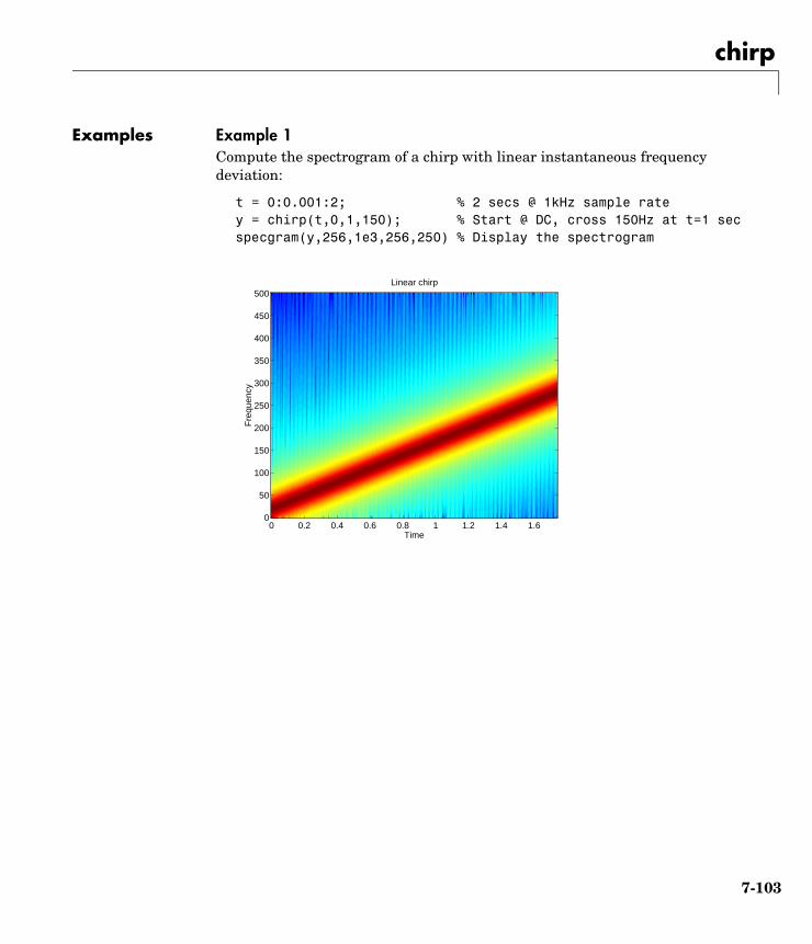
chirp
Examples Example 1Compute the spectrogram of a chirp with linear instantaneous frequency deviation:
t = 0:0.001:2; % 2 secs @ 1kHz sample ratey = chirp(t,0,1,150); % Start @ DC, cross 150Hz at t=1 secspecgram(y,256,1e3,256,250) % Display the spectrogram
Time
Fre
quen
cy
Linear chirp
0 0.2 0.4 0.6 0.8 1 1.2 1.4 1.60
50
100
150
200
250
300
350
400
450
500
7-103
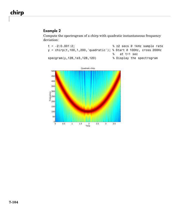
chirp
Example 2Compute the spectrogram of a chirp with quadratic instantaneous frequency deviation:
t = -2:0.001:2; % ±2 secs @ 1kHz sample ratey = chirp(t,100,1,200,'quadratic'); % Start @ 100Hz, cross 200Hz
% at t=1 secspecgram(y,128,1e3,128,120) % Display the spectrogram
Time
Fre
quen
cy
Quadratic chirp
0 0.5 1 1.5 2 2.5 3 3.50
50
100
150
200
250
300
350
400
450
500
7-104
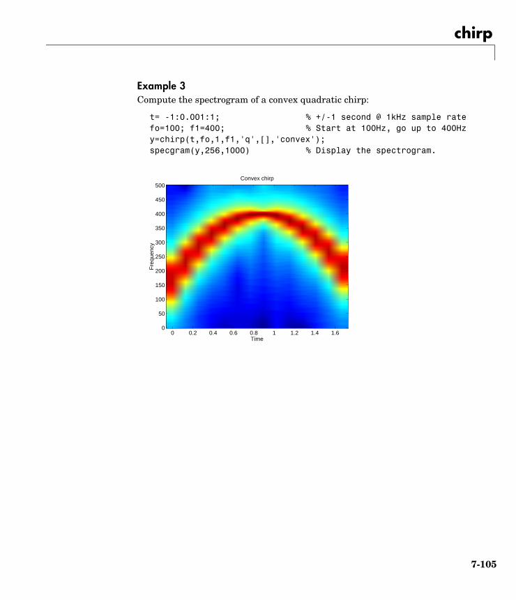
chirp
Example 3Compute the spectrogram of a convex quadratic chirp:
t= -1:0.001:1; % +/-1 second @ 1kHz sample ratefo=100; f1=400; % Start at 100Hz, go up to 400Hzy=chirp(t,fo,1,f1,'q',[],'convex');specgram(y,256,1000) % Display the spectrogram.
Time
Fre
quen
cy
Convex chirp
0 0.2 0.4 0.6 0.8 1 1.2 1.4 1.60
50
100
150
200
250
300
350
400
450
500
7-105
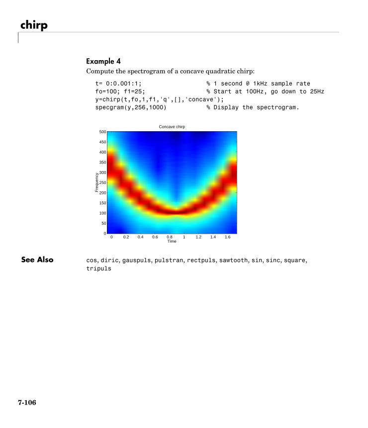
chirp
Example 4Compute the spectrogram of a concave quadratic chirp:
t= 0:0.001:1; % 1 second @ 1kHz sample ratefo=100; f1=25; % Start at 100Hz, go down to 25Hzy=chirp(t,fo,1,f1,'q',[],'concave');specgram(y,256,1000) % Display the spectrogram.
See Also cos, diric, gauspuls, pulstran, rectpuls, sawtooth, sin, sinc, square, tripuls
Time
Fre
quen
cy
Concave chirp
0 0.2 0.4 0.6 0.8 1 1.2 1.4 1.60
50
100
150
200
250
300
350
400
450
500
7-106

conv
7convPurpose Convolution and polynomial multiplication
conv is a MATLAB function.
7-107

conv2
7conv2Purpose Two-dimensional convolution
conv2 is a MATLAB function.
7-108
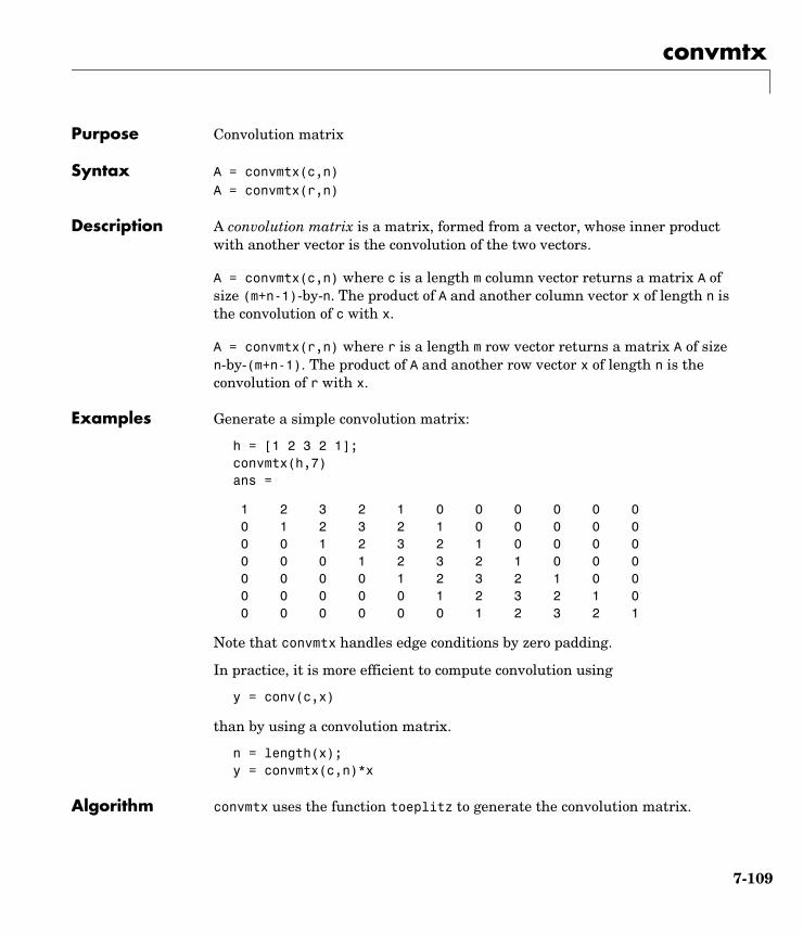
convmtx
7convmtxPurpose Convolution matrix
Syntax A = convmtx(c,n)A = convmtx(r,n)
Description A convolution matrix is a matrix, formed from a vector, whose inner product with another vector is the convolution of the two vectors.
A = convmtx(c,n) where c is a length m column vector returns a matrix A of size (m+n-1)-by-n. The product of A and another column vector x of length n is the convolution of c with x.
A = convmtx(r,n) where r is a length m row vector returns a matrix A of size n-by-(m+n-1). The product of A and another row vector x of length n is the convolution of r with x.
Examples Generate a simple convolution matrix:
h = [1 2 3 2 1];convmtx(h,7)ans =
1 2 3 2 1 0 0 0 0 0 0 0 1 2 3 2 1 0 0 0 0 0 0 0 1 2 3 2 1 0 0 0 0 0 0 0 1 2 3 2 1 0 0 0 0 0 0 0 1 2 3 2 1 0 0 0 0 0 0 0 1 2 3 2 1 0 0 0 0 0 0 0 1 2 3 2 1
Note that convmtx handles edge conditions by zero padding.
In practice, it is more efficient to compute convolution using
y = conv(c,x)
than by using a convolution matrix.
n = length(x);y = convmtx(c,n)*x
Algorithm convmtx uses the function toeplitz to generate the convolution matrix.
7-109

convmtx
See Also conv, convn, conv2, dftmtx
7-110

corrcoef
7corrcoefPurpose Compute the correlation coefficient matrix
corrcoef is a MATLAB function.
7-111
corrmtx
7corrmtxPurpose Compute a data matrix for autocorrelation matrix estimation
Syntax X = corrmtx(x,m)X = corrmtx(x,m,'method')[X,R] = corrmtx(...)
Description X = corrmtx(x,m) returns an (n+m)-by-(m+1) rectangular Toeplitz matrix X, such that X'X is a (biased) estimate of the autocorrelation matrix for the length n data vector x.
X = corrmtx(x,m,'method') computes the matrix X according to the method specified by the string 'method':
• 'autocorrelation': (default) X is the (n+m)-by-(m+1) rectangular Toeplitz matrix that generates an autocorrelation estimate for the length n data vector x, derived using prewindowed and postwindowed data, based on an mth order prediction error model.
• 'prewindowed': X is the n-by-(m+1) rectangular Toeplitz matrix that generates an autocorrelation estimate for the length n data vector x, derived using prewindowed data, based on an mth order prediction error model.
• 'postwindowed': X is the n-by-(m+1) rectangular Toeplitz matrix that generates an autocorrelation estimate for the length n data vector x, derived using postwindowed data, based on an mth order prediction error model.
• 'covariance': X is the (n-m)-by-(m+1) rectangular Toeplitz matrix that generates an autocorrelation estimate for the length n data vector x, derived using nonwindowed data, based on an mth order prediction error model.
• 'modified': X is the 2(n-m)-by-(m+1) modified rectangular Toeplitz matrix that generates an autocorrelation estimate for the length n data vector x, derived using forward and backward prediction error estimates, based on an mth order prediction error model.
[X,R] = corrmtx(...) also returns the (m+1)-by-(m+1) autocorrelation matrix estimate R, calculated as X'*X.
Examples randn('state',1); n=0:99; s=exp(i*pi/2*n)+2*exp(i*pi/4*n)+exp(i*pi/3*n)+randn(1,100); X=corrmtx(s,12,'mod');
7-112
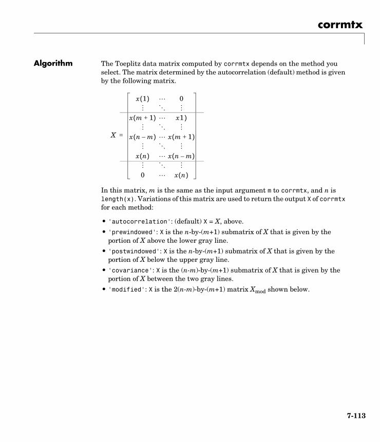
corrmtx
Algorithm The Toeplitz data matrix computed by corrmtx depends on the method you select. The matrix determined by the autocorrelation (default) method is given by the following matrix.
In this matrix, m is the same as the input argument m to corrmtx, and n is length(x). Variations of this matrix are used to return the output X of corrmtx for each method:
• 'autocorrelation': (default) X = X, above.
• 'prewindowed': X is the n-by-(m+1) submatrix of X that is given by the portion of X above the lower gray line.
• 'postwindowed': X is the n-by-(m+1) submatrix of X that is given by the portion of X below the upper gray line.
• 'covariance': X is the (n-m)-by-(m+1) submatrix of X that is given by the portion of X between the two gray lines.
• 'modified': X is the 2(n-m)-by-(m+1) matrix Xmod shown below.
X
x 1( ) 0
x m 1+( ) x1 )
x n m–( ) x m 1+( )
x n( ) x n m–( )
0 x n( )
=
7-113
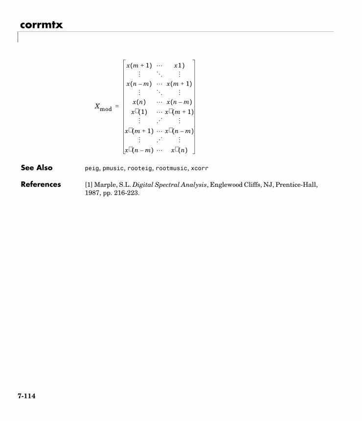
corrmtx
See Also peig, pmusic, rooteig, rootmusic, xcorr
References [1] Marple, S.L. Digital Spectral Analysis, Englewood Cliffs, NJ, Prentice-Hall, 1987, pp. 216-223.
Xmod
x m 1+( ) x1 )
x n m–( ) x m 1+( )
x n( ) x n m–( )x∗ 1( ) x∗ m 1+( )
x∗ m 1+( ) x∗ n m–( )
x∗ n m–( ) x∗ n( )
=
7-114

cov
7covPurpose Compute the covariance matrix
cov is a MATLAB function.
7-115

cplxpair
7cplxpairPurpose Group complex numbers into complex conjugate pairs
cplxpair is a MATLAB function.
7-116
cpsd
7cpsdPurpose Estimate the cross power spectral density (CPSD) of two signals
Syntax Pxy = cpsd(x,y)Pxy = cpsd(x,y,window)Pxy = cpsd(x,y,window,noverlap)[Pxy,W] = cpsd(x,y,window,noverlap,nfft)[Pxy,F] = cpsd(x,y,window,noverlap,nfft,fs)[...] = cpsd(..., twosided )cpsd(x,y,...)
Description Pxy = cpsd(x,y) estimates the cross power spectral density Pxy of the discrete-time signals x and y using the Welch’s averaged, modified periodogram method of spectral estimation. The cross power spectral density is the distribution of power per unit frequency.
For real x and y, cpsd returns a one-sided CPSD and for complex x or y, it returns a two-sided CPSD.
7-117
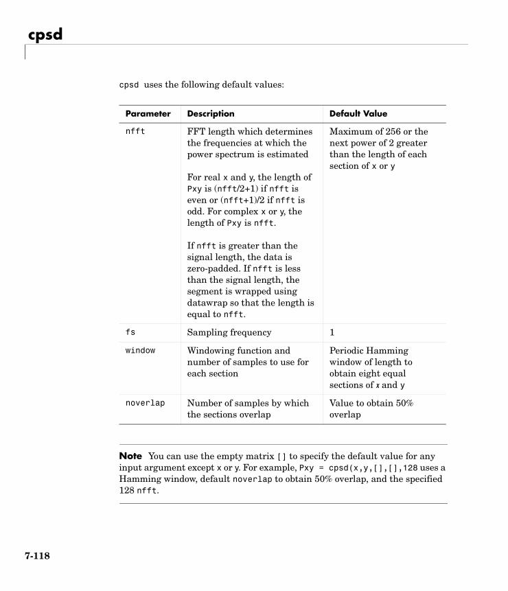
cpsd
cpsd uses the following default values:
Note You can use the empty matrix [] to specify the default value for any input argument except x or y. For example, Pxy = cpsd(x,y,[],[],128 uses a Hamming window, default noverlap to obtain 50% overlap, and the specified 128 nfft.
Parameter Description Default Value
nfft FFT length which determines the frequencies at which the power spectrum is estimated
For real x and y, the length of Pxy is (nfft/2+1) if nfft is even or (nfft+1)/2 if nfft is odd. For complex x or y, the length of Pxy is nfft.
If nfft is greater than the signal length, the data is zero-padded. If nfft is less than the signal length, the segment is wrapped using datawrap so that the length is equal to nfft.
Maximum of 256 or the next power of 2 greater than the length of each section of x or y
fs Sampling frequency 1
window Windowing function and number of samples to use for each section
Periodic Hamming window of length to obtain eight equal sections of x and y
noverlap Number of samples by which the sections overlap
Value to obtain 50% overlap
7-118
cpsd
Pxy = cpsd(x,y,window) specifies a windowing function, divides x and y into overlapping sections of the specified window length, and windows each section using the specified window function. If you supply a scalar for window, Pxy uses a Hamming window of that length. The x and y vectors are divided into eight equal sections of that length. If the signal cannot be sectioned evenly with 50% overlap, it is truncated.
Pxy = cpsd(x,y,window,noverlap) overlaps the sections of x by noverlap samples. noverlap must be an integer smaller than the length of window.
[Pxy,W] = cpsd(x,y,window,noverlap,nfft) uses the specified FFT length nfft in estimating the CPSD. It also returns W, which is the vector of normalized frequencies (in rad/sample) at which the CPSD is estimated. For real signals, the range of W is [0, pi] when nfft is even and [0, pi) when nfft is odd. For complex signals, the range of W is [0, 2*pi).
[Pxy,F] = cpsd(x,y,window,noverlap,nfft,fs) returns Pxy as a function of frequency and a vector F of frequencies at which the CPSD is estimated. fs is the sampling frequency in Hz. For real signals, the range of F is [0, fs/2] when nfft is even and [0, fs/2) when nfft is odd. For complex signals, the range of F is [0, fs).
[...] = cpsd(..., twosided ) returns the two-sided CPSD of real signals x and y. The length of the resulting Pxy is nfft and its range is [0, 2*pi) if you do not specify fs. If you specify fs, the range is [0,fs). Entering onesided for a real signal produces the default. You can place the onesided or twosided string in any position after the noverlap parameter.
cpsd(...) plots the CPSD versus frequency in the current figure window.
Examples Generate two colored noise signals and plot their CPSD with a confidence interval of 95%. Specify a length 1024 FFT, a 500 point triangular window with no overlap, and a sampling frequency of 10 Hz:
randn('state',0);h = fir1(30,0.2,rectwin(31));h1 = ones(1,10)/sqrt(10);r = randn(16384,1);x = filter(h1,1,r);y = filter(h,1,x);
7-119
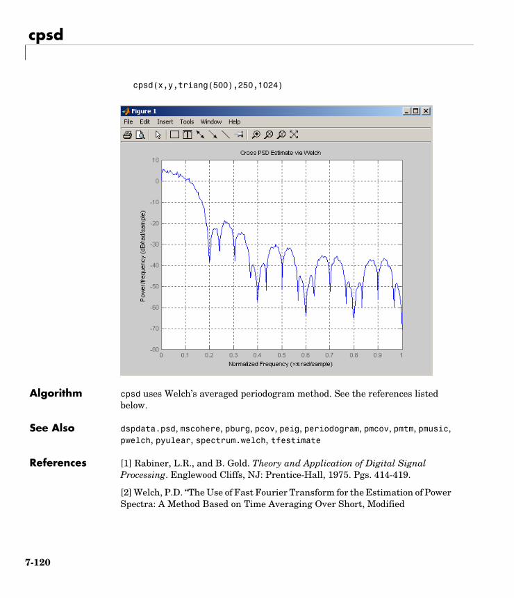
cpsd
cpsd(x,y,triang(500),250,1024)
Algorithm cpsd uses Welch’s averaged periodogram method. See the references listed below.
See Also dspdata.psd, mscohere, pburg, pcov, peig, periodogram, pmcov, pmtm, pmusic, pwelch, pyulear, spectrum.welch, tfestimate
References [1] Rabiner, L.R., and B. Gold. Theory and Application of Digital Signal Processing. Englewood Cliffs, NJ: Prentice-Hall, 1975. Pgs. 414-419.
[2] Welch, P.D. “The Use of Fast Fourier Transform for the Estimation of Power Spectra: A Method Based on Time Averaging Over Short, Modified
7-120
cpsd
Periodograms.” IEEE Trans. Audio Electroacoust. Vol. AU-15 (June 1967). Pgs. 70-73.
[3] Oppenheim, A.V., and R.W. Schafer. Discrete-Time Signal Processing. Upper Saddle River, NJ: Prentice-Hall, 1999, pp. 737.
7-121
czt
7cztPurpose Chirp z-transform
Syntax y = czt(x,m,w,a)y = czt(x)
Description y = czt(x,m,w,a) returns the chirp z-transform of signal x. The chirp z-transform is the z-transform of x along a spiral contour defined by w and a. m is a scalar that specifies the length of the transform, w is the ratio between points along the z-plane spiral contour of interest, and scalar a is the complex starting point on that contour. The contour, a spiral or “chirp” in the z-plane, is given by
z = a*(w.^-(0:m-1))
y = czt(x) uses the following default values:
• m = length(x)
• w = exp(j*2*pi/m)
• a = 1
With these defaults, czt returns the z-transform of x at m equally spaced points around the unit circle. This is equivalent to the discrete Fourier transform of x, or fft(x). The empty matrix [] specifies the default value for a parameter.
If x is a matrix, czt(x,m,w,a) transforms the columns of x.
Examples Create a random vector x of length 1013 and compute its DFT using czt:
randn('state',0);x = randn(1013,1);y = czt(x);
Use czt to zoom in on a narrow-band section (100 to 150 Hz) of a filter’s frequency response. First design the filter:
h = fir1(30,125/500,rectwin(31)); % filter
7-122
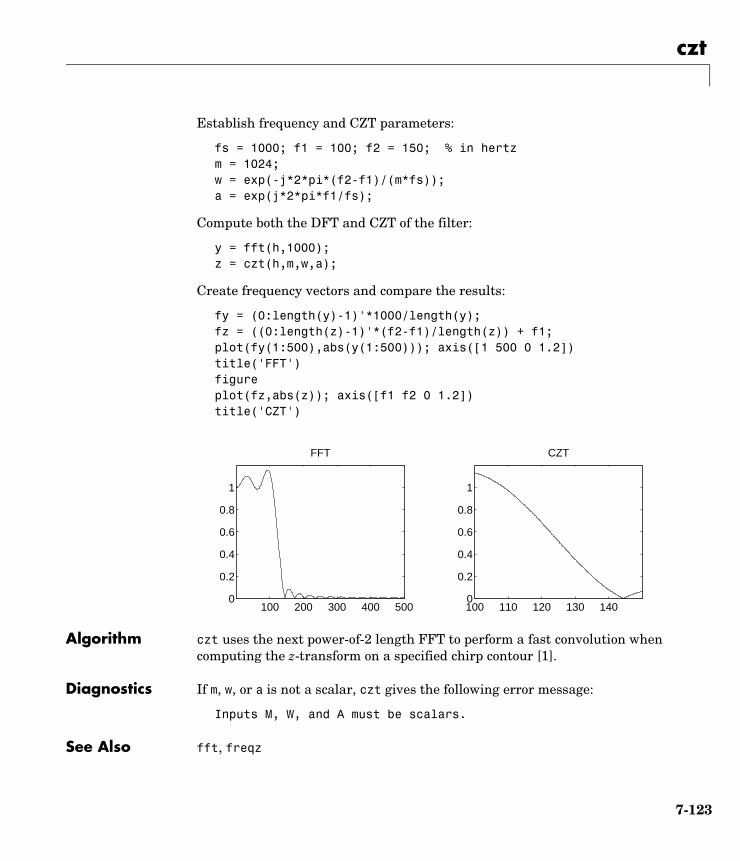
czt
Establish frequency and CZT parameters:
fs = 1000; f1 = 100; f2 = 150; % in hertzm = 1024;w = exp(-j*2*pi*(f2-f1)/(m*fs));a = exp(j*2*pi*f1/fs);
Compute both the DFT and CZT of the filter:
y = fft(h,1000);z = czt(h,m,w,a);
Create frequency vectors and compare the results:
fy = (0:length(y)-1)'*1000/length(y); fz = ((0:length(z)-1)'*(f2-f1)/length(z)) + f1;plot(fy(1:500),abs(y(1:500))); axis([1 500 0 1.2])title('FFT')figureplot(fz,abs(z)); axis([f1 f2 0 1.2])title('CZT')
Algorithm czt uses the next power-of-2 length FFT to perform a fast convolution when computing the z-transform on a specified chirp contour [1].
Diagnostics If m, w, or a is not a scalar, czt gives the following error message:
Inputs M, W, and A must be scalars.
See Also fft, freqz
100 200 300 400 5000
0.2
0.4
0.6
0.8
1
FFT
100 110 120 130 1400
0.2
0.4
0.6
0.8
1
CZT
7-123

czt
References [1] Rabiner, L.R., and B. Gold. Theory and Application of Digital Signal Processing. Englewood Cliffs, NJ: Prentice-Hall, 1975. Pgs. 393-399.
7-124
dct
7dctPurpose Discrete cosine transform (DCT)
Syntax y = dct(x)y = dct(x,n)
Description y = dct(x) returns the unitary discrete cosine transform of x
where
N is the length of x, and x and y are the same size. If x is a matrix, dct transforms its columns. The series is indexed from n = 1 and k = 1 instead of the usual n = 0 and k = 0 because MATLAB vectors run from 1 to N instead of from 0 to N- 1.
y = dct(x,n) pads or truncates x to length n before transforming.
The DCT is closely related to the discrete Fourier transform. You can often reconstruct a sequence very accurately from only a few DCT coefficients, a useful property for applications requiring data reduction.
y k( ) w k( ) x n( )π 2n 1–( ) k 1–( )
2N-------------------------------------------cos
n 1=
N
∑ k 1 … N, ,=,=
w k( )
1N
--------- k 1=,
2N---- 2 k N≤ ≤,
=
7-125

dct
Examples Find how many DCT coefficients represent 99% of the energy in a sequence:
x = (1:100) + 50*cos((1:100)*2*pi/40);X = dct(x);[XX,ind] = sort(abs(X)); ind = fliplr(ind);i = 1;while (norm([X(ind(1:i)) zeros(1,100-i)])/norm(X)<.99)
i = i + 1;end
i = 3
See Also fft, idct, dct2, idct2
References [1] Jain, A.K. Fundamentals of Digital Image Processing. Englewood Cliffs, NJ: Prentice-Hall, 1989.
[2] Pennebaker, W.B., and J.L. Mitchell. JPEG Still Image Data Compression Standard. New York, NY: Van Nostrand Reinhold, 1993. Chapter 4.
7-126
decimate
7decimatePurpose Decrease the sampling rate for a sequence (decimation)
Syntax y = decimate(x,r)y = decimate(x,r,n)y = decimate(x,r,'fir')y = decimate(x,r,n,'fir')
Description Decimation reduces the original sampling rate for a sequence to a lower rate, the opposite of interpolation. The decimation process filters the input data with a lowpass filter and then resamples the resulting smoothed signal at a lower rate.
y = decimate(x,r) reduces the sample rate of x by a factor r. The decimated vector y is r times shorter in length than the input vector x. By default, decimate employs an eighth-order lowpass Chebyshev Type I filter. It filters the input sequence in both the forward and reverse directions to remove all phase distortion, effectively doubling the filter order.
y = decimate(x,r,n) uses an order n Chebyshev filter. Orders above 13 are not recommended because of numerical instability. MATLAB displays a warning in this case.
y = decimate(x,r,'fir') uses a 30-point FIR filter, instead of the Chebyshev IIR filter. Here decimate filters the input sequence in only one direction. This technique conserves memory and is useful for working with long sequences.
y = decimate(x,r,n,'fir') uses a length n FIR filter.
Examples Decimate a signal by a factor of four:
t = 0:.00025:1; % Time vectorx = sin(2*pi*30*t) + sin(2*pi*60*t);y = decimate(x,4);
7-127
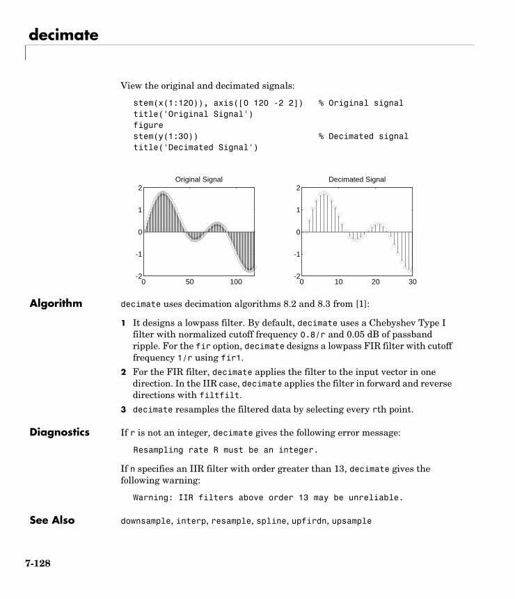
decimate
View the original and decimated signals:
stem(x(1:120)), axis([0 120 -2 2]) % Original signaltitle('Original Signal')figurestem(y(1:30)) % Decimated signaltitle('Decimated Signal')
Algorithm decimate uses decimation algorithms 8.2 and 8.3 from [1]:
1 It designs a lowpass filter. By default, decimate uses a Chebyshev Type I filter with normalized cutoff frequency 0.8/r and 0.05 dB of passband ripple. For the fir option, decimate designs a lowpass FIR filter with cutoff frequency 1/r using fir1.
2 For the FIR filter, decimate applies the filter to the input vector in one direction. In the IIR case, decimate applies the filter in forward and reverse directions with filtfilt.
3 decimate resamples the filtered data by selecting every rth point.
Diagnostics If r is not an integer, decimate gives the following error message:
Resampling rate R must be an integer.
If n specifies an IIR filter with order greater than 13, decimate gives the following warning:
Warning: IIR filters above order 13 may be unreliable.
See Also downsample, interp, resample, spline, upfirdn, upsample
0 50 100-2
-1
0
1
2Original Signal
0 10 20 30-2
-1
0
1
2Decimated Signal
7-128

decimate
References [1] IEEE. Programs for Digital Signal Processing. IEEE Press. New York: John Wiley & Sons, 1979. Chapter 8.
7-129

deconv
7deconvPurpose Deconvolution and polynomial division
deconv is a MATLAB function.
7-130
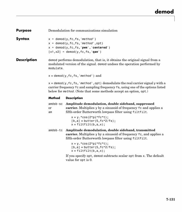
demod
7demodPurpose Demodulation for communications simulation
Syntax x = demod(y,fc,fs,'method')x = demod(y,fc,fs,'method',opt)x = demod(y,fc,fs,'pwm','centered')[x1,x2] = demod(y,fc,fs,'qam')
Description demod performs demodulation, that is, it obtains the original signal from a modulated version of the signal. demod undoes the operation performed by modulate.
x = demod(y,fc,fs,'method') and
x = demod(y,fc,fs,'method',opt) demodulate the real carrier signal y with a carrier frequency fc and sampling frequency fs, using one of the options listed below for method. (Note that some methods accept an option, opt.)
Method Description
amdsb-scoram
Amplitude demodulation, double sideband, suppressed carrier. Multiplies y by a sinusoid of frequency fc and applies a fifth-order Butterworth lowpass filter using filtfilt.
x = y.*cos(2*pi*fc*t);[b,a] = butter(5,fc*2/fs);x = filtfilt(b,a,x);
amdsb-tc Amplitude demodulation, double sideband, transmitted carrier. Multiplies y by a sinusoid of frequency fc, and applies a fifth-order Butterworth lowpass filter using filtfilt.
x = y.*cos(2*pi*fc*t);[b,a] = butter(5,fc*2/fs);x = filtfilt(b,a,x);
If you specify opt, demod subtracts scalar opt from x. The default value for opt is 0.
7-131
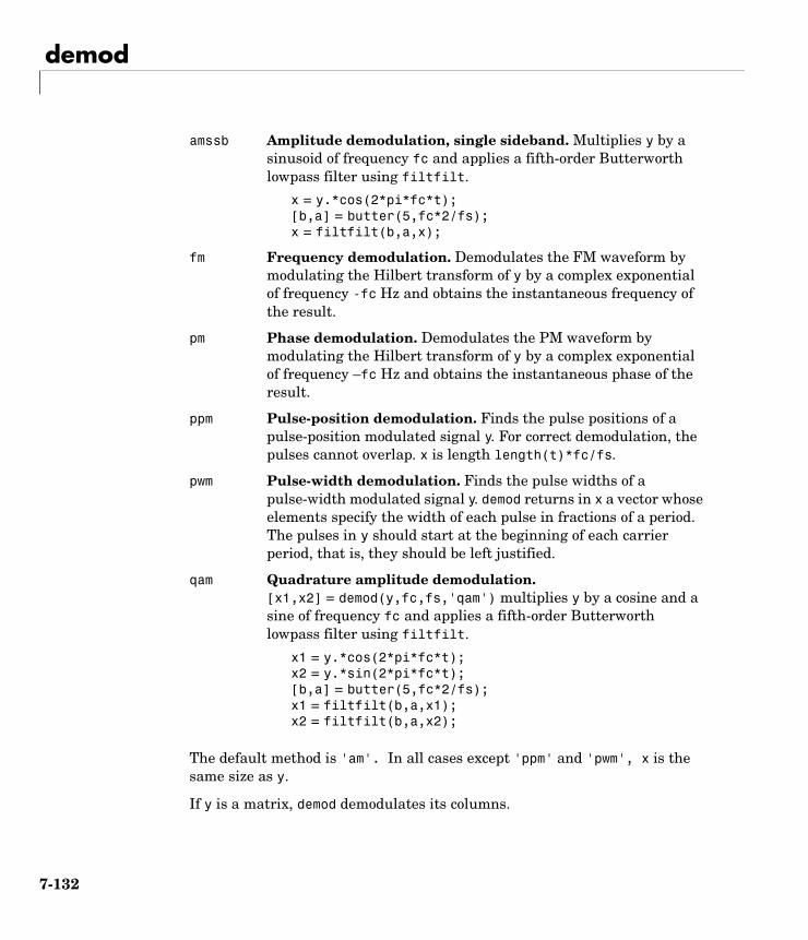
demod
The default method is 'am'. In all cases except 'ppm' and 'pwm', x is the same size as y.
If y is a matrix, demod demodulates its columns.
amssb Amplitude demodulation, single sideband. Multiplies y by a sinusoid of frequency fc and applies a fifth-order Butterworth lowpass filter using filtfilt.
x = y.*cos(2*pi*fc*t);[b,a] = butter(5,fc*2/fs);x = filtfilt(b,a,x);
fm Frequency demodulation. Demodulates the FM waveform by modulating the Hilbert transform of y by a complex exponential of frequency -fc Hz and obtains the instantaneous frequency of the result.
pm Phase demodulation. Demodulates the PM waveform by modulating the Hilbert transform of y by a complex exponential of frequency –fc Hz and obtains the instantaneous phase of the result.
ppm Pulse-position demodulation. Finds the pulse positions of a pulse-position modulated signal y. For correct demodulation, the pulses cannot overlap. x is length length(t)*fc/fs.
pwm Pulse-width demodulation. Finds the pulse widths of a pulse-width modulated signal y. demod returns in x a vector whose elements specify the width of each pulse in fractions of a period. The pulses in y should start at the beginning of each carrier period, that is, they should be left justified.
qam Quadrature amplitude demodulation.[x1,x2] = demod(y,fc,fs,'qam') multiplies y by a cosine and a sine of frequency fc and applies a fifth-order Butterworth lowpass filter using filtfilt.
x1 = y.*cos(2*pi*fc*t);x2 = y.*sin(2*pi*fc*t);[b,a] = butter(5,fc*2/fs);x1 = filtfilt(b,a,x1);x2 = filtfilt(b,a,x2);
7-132

demod
x = demod(y,fc,fs,'pwm','centered') finds the pulse widths assuming they are centered at the beginning of each period. x is length length(y)*fc/fs.
See Also modulate, vco, fskdemod, genqamdemod, mskdemod, pamdemod, pmdemod, qamdemod
7-133
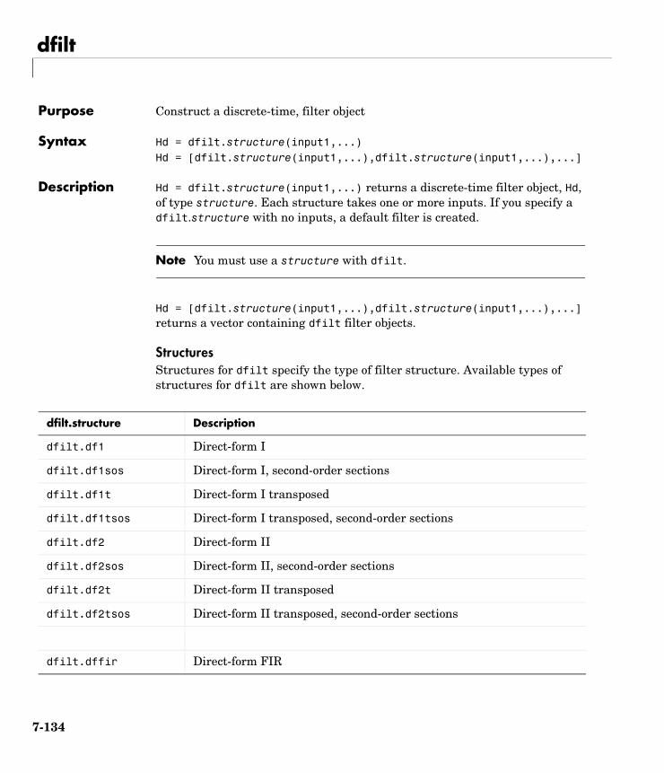
dfilt
7dfiltPurpose Construct a discrete-time, filter object
Syntax Hd = dfilt.structure(input1,...)Hd = [dfilt.structure(input1,...),dfilt.structure(input1,...),...]
Description Hd = dfilt.structure(input1,...) returns a discrete-time filter object, Hd, of type structure. Each structure takes one or more inputs. If you specify a dfilt.structure with no inputs, a default filter is created.
Note You must use a structure with dfilt.
Hd = [dfilt.structure(input1,...),dfilt.structure(input1,...),...] returns a vector containing dfilt filter objects.
StructuresStructures for dfilt specify the type of filter structure. Available types of structures for dfilt are shown below.
dfilt.structure Description
dfilt.df1 Direct-form I
dfilt.df1sos Direct-form I, second-order sections
dfilt.df1t Direct-form I transposed
dfilt.df1tsos Direct-form I transposed, second-order sections
dfilt.df2 Direct-form II
dfilt.df2sos Direct-form II, second-order sections
dfilt.df2t Direct-form II transposed
dfilt.df2tsos Direct-form II transposed, second-order sections
dfilt.dffir Direct-form FIR
7-134
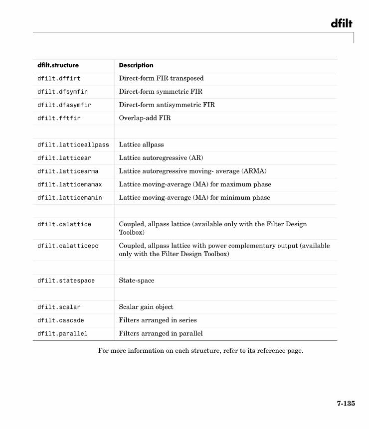
dfilt
For more information on each structure, refer to its reference page.
dfilt.dffirt Direct-form FIR transposed
dfilt.dfsymfir Direct-form symmetric FIR
dfilt.dfasymfir Direct-form antisymmetric FIR
dfilt.fftfir Overlap-add FIR
dfilt.latticeallpass Lattice allpass
dfilt.latticear Lattice autoregressive (AR)
dfilt.latticearma Lattice autoregressive moving- average (ARMA)
dfilt.latticemamax Lattice moving-average (MA) for maximum phase
dfilt.latticemamin Lattice moving-average (MA) for minimum phase
dfilt.calattice Coupled, allpass lattice (available only with the Filter Design Toolbox)
dfilt.calatticepc Coupled, allpass lattice with power complementary output (available only with the Filter Design Toolbox)
dfilt.statespace State-space
dfilt.scalar Scalar gain object
dfilt.cascade Filters arranged in series
dfilt.parallel Filters arranged in parallel
dfilt.structure Description
7-135
dfilt
MethodsMethods provide ways of performing functions directly on your dfilt object without having to specify the filter parameters again. You can apply these methods directly on the variable you assigned to your dfilt object.
For example, if you create a dfilt object, Hd, you can check whether it has linear phase with islinphase(Hd), view its frequency response plot with fvtool(Hd), or obtain its frequency response values with h=freqz(Hd). You can use all of the methods below in this way.
Note If your variable is a 1-D array dfilt filter objects, the method is applied to each object in the array. Only freqz, grpdelay, impz, is*, order, and stepz methods can be applied to arrays. The zplane method can be applied to an array only if it is used without outputs.
7-136
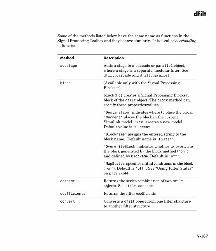
dfilt
Some of the methods listed below have the same name as functions in the Signal Processing Toolbox and they behave similarly. This is called overloading of functions.
Method Description
addstage Adds a stage to a cascade or parallel object, where a stage is a separate, modular filter. See dfilt.cascade and dfilt.parallel.
block (Available only with the Signal Processing Blockset)
block(Hd) creates a Signal Processing Blockset block of the dfilt object. The block method can specify these properties/values:
'Destination' indicates where to place the block. 'Current' places the block in the current Simulink model. 'New' creates a new model. Default value is 'Current'.
'Blockname' assigns the entered string to the block name. Default name is 'Filter'.
'OverwriteBlock'indicates whether to overwrite the block generated by the block method ('on') and defined by Blockame. Default is 'off'.
'MapStates' specifies initial conditions in the block ('on'). Default is 'off'. See “Using Filter States” on page 7-144.
cascade Returns the series combination of two dfilt objects. See dfilt.cascade.
coefficients Returns the filter coefficients
convert Converts a dfilt object from one filter structure to another filter structure
7-137
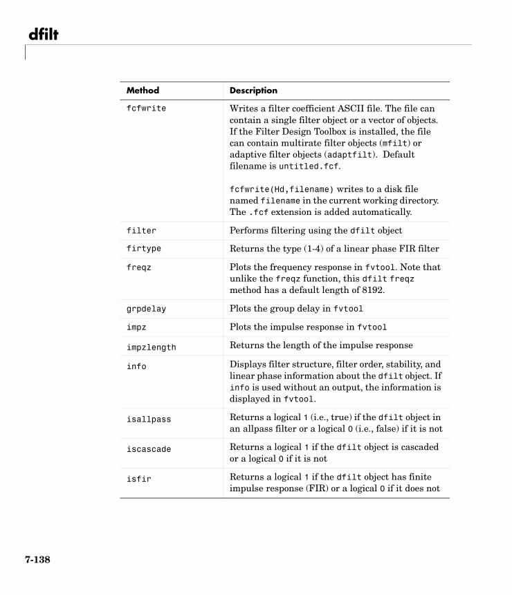
dfilt
fcfwrite Writes a filter coefficient ASCII file. The file can contain a single filter object or a vector of objects. If the Filter Design Toolbox is installed, the file can contain multirate filter objects (mfilt) or adaptive filter objects (adaptfilt). Default filename is untitled.fcf.
fcfwrite(Hd,filename) writes to a disk file named filename in the current working directory. The .fcf extension is added automatically.
filter Performs filtering using the dfilt object
firtype Returns the type (1-4) of a linear phase FIR filter
freqz Plots the frequency response in fvtool. Note that unlike the freqz function, this dfilt freqz method has a default length of 8192.
grpdelay Plots the group delay in fvtool
impz Plots the impulse response in fvtool
impzlength Returns the length of the impulse response
info Displays filter structure, filter order, stability, and linear phase information about the dfilt object. If info is used without an output, the information is displayed in fvtool.
isallpass Returns a logical 1 (i.e., true) if the dfilt object in an allpass filter or a logical 0 (i.e., false) if it is not
iscascade Returns a logical 1 if the dfilt object is cascaded or a logical 0 if it is not
isfir Returns a logical 1 if the dfilt object has finite impulse response (FIR) or a logical 0 if it does not
Method Description
7-138
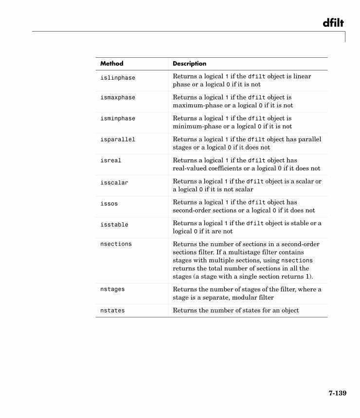
dfilt
islinphase Returns a logical 1 if the dfilt object is linear phase or a logical 0 if it is not
ismaxphase Returns a logical 1 if the dfilt object is maximum-phase or a logical 0 if it is not
isminphase Returns a logical 1 if the dfilt object is minimum-phase or a logical 0 if it is not
isparallel Returns a logical 1 if the dfilt object has parallel stages or a logical 0 if it does not
isreal Returns a logical 1 if the dfilt object has real-valued coefficients or a logical 0 if it does not
isscalar Returns a logical 1 if the dfilt object is a scalar or a logical 0 if it is not scalar
issos Returns a logical 1 if the dfilt object has second-order sections or a logical 0 if it does not
isstable Returns a logical 1 if the dfilt object is stable or a logical 0 if it are not
nsections Returns the number of sections in a second-order sections filter. If a multistage filter contains stages with multiple sections, using nsections returns the total number of sections in all the stages (a stage with a single section returns 1).
nstages Returns the number of stages of the filter, where a stage is a separate, modular filter
nstates Returns the number of states for an object
Method Description
7-139
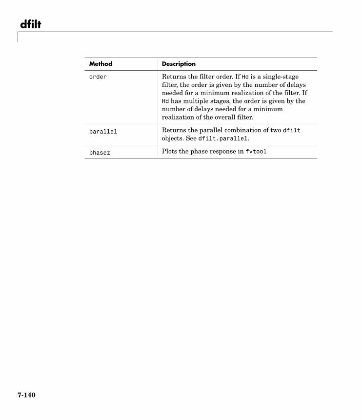
dfilt
order Returns the filter order. If Hd is a single-stage filter, the order is given by the number of delays needed for a minimum realization of the filter. If Hd has multiple stages, the order is given by the number of delays needed for a minimum realization of the overall filter.
parallel Returns the parallel combination of two dfilt objects. See dfilt.parallel.
phasez Plots the phase response in fvtool
Method Description
7-140
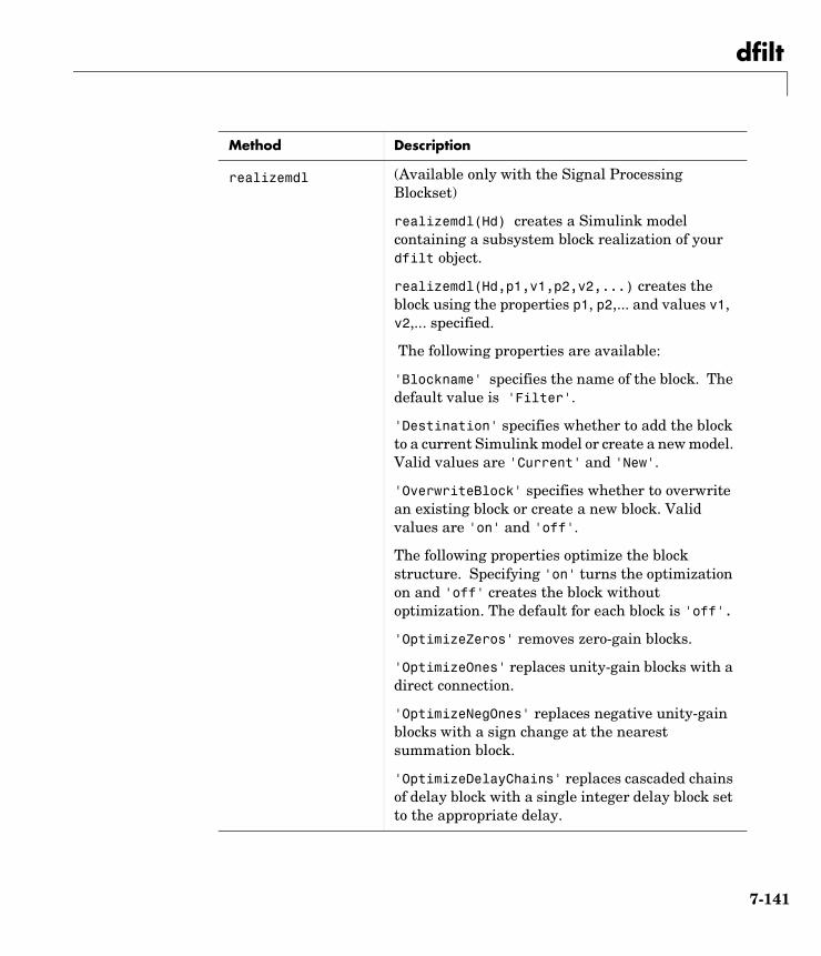
dfilt
realizemdl (Available only with the Signal Processing Blockset)
realizemdl(Hd) creates a Simulink model containing a subsystem block realization of your dfilt object.
realizemdl(Hd,p1,v1,p2,v2,...) creates the block using the properties p1, p2,... and values v1, v2,... specified.
The following properties are available:
'Blockname' specifies the name of the block. The default value is 'Filter'.
'Destination' specifies whether to add the block to a current Simulink model or create a new model. Valid values are 'Current' and 'New'.
'OverwriteBlock' specifies whether to overwrite an existing block or create a new block. Valid values are 'on' and 'off'.
The following properties optimize the block structure. Specifying 'on' turns the optimization on and 'off' creates the block without optimization. The default for each block is 'off'.
'OptimizeZeros' removes zero-gain blocks.
'OptimizeOnes' replaces unity-gain blocks with a direct connection.
'OptimizeNegOnes' replaces negative unity-gain blocks with a sign change at the nearest summation block.
'OptimizeDelayChains' replaces cascaded chains of delay block with a single integer delay block set to the appropriate delay.
Method Description
7-141
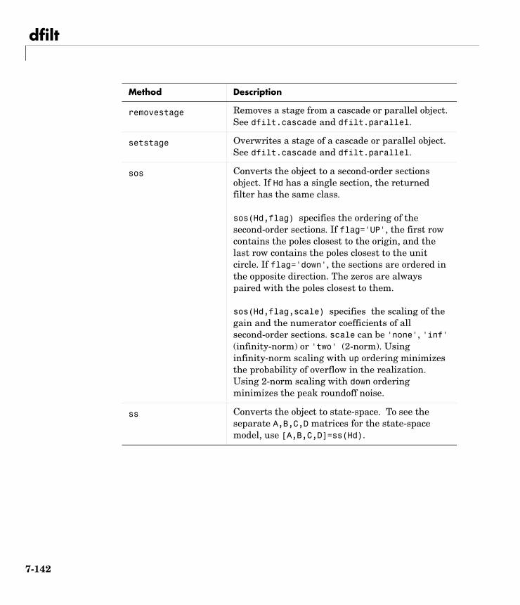
dfilt
removestage Removes a stage from a cascade or parallel object. See dfilt.cascade and dfilt.parallel.
setstage Overwrites a stage of a cascade or parallel object. See dfilt.cascade and dfilt.parallel.
sos Converts the object to a second-order sections object. If Hd has a single section, the returned filter has the same class.
sos(Hd,flag) specifies the ordering of the second-order sections. If flag='UP', the first row contains the poles closest to the origin, and the last row contains the poles closest to the unit circle. If flag='down', the sections are ordered in the opposite direction. The zeros are always paired with the poles closest to them. sos(Hd,flag,scale) specifies the scaling of the gain and the numerator coefficients of all second-order sections. scale can be 'none', 'inf' (infinity-norm) or 'two' (2-norm). Using infinity-norm scaling with up ordering minimizes the probability of overflow in the realization. Using 2-norm scaling with down ordering minimizes the peak roundoff noise.
ss Converts the object to state-space. To see the separate A,B,C,D matrices for the state-space model, use [A,B,C,D]=ss(Hd).
Method Description
7-142
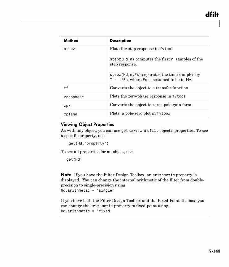
dfilt
Viewing Object PropertiesAs with any object, you can use get to view a dfilt object’s properties. To see a specific property, use
get(Hd,'property')
To see all properties for an object, use
get(Hd)
Note If you have the Filter Design Toolbox, an arithmetic property is displayed. You can change the internal arithmetic of the filter from double- precision to single-precision using:Hd.arithmetic = 'single'
If you have both the Filter Design Toolbox and the Fixed-Point Toolbox, you can change the arithmetic property to fixed-point using:Hd.arithmetic = 'fixed'
stepz Plots the step response in fvtool
stepz(Hd,n) computes the first n samples of the step response.
stepz(Hd,n,Fs) separates the time samples by T = 1/Fs, where Fs is assumed to be in Hz.
tf Converts the object to a transfer function
zerophase Plots the zero-phase response in fvtool
zpk Converts the object to zeros-pole-gain form
zplane Plots a pole-zero plot in fvtool
Method Description
7-143
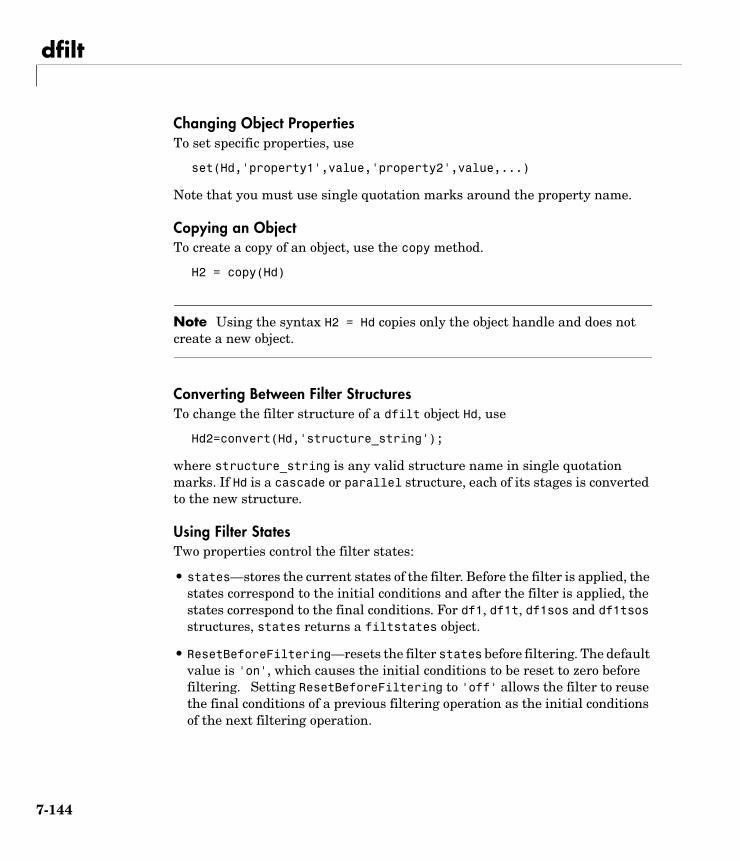
dfilt
Changing Object PropertiesTo set specific properties, use
set(Hd,'property1',value,'property2',value,...)
Note that you must use single quotation marks around the property name.
Copying an ObjectTo create a copy of an object, use the copy method.
H2 = copy(Hd)
Note Using the syntax H2 = Hd copies only the object handle and does not create a new object.
Converting Between Filter StructuresTo change the filter structure of a dfilt object Hd, use
Hd2=convert(Hd,'structure_string');
where structure_string is any valid structure name in single quotation marks. If Hd is a cascade or parallel structure, each of its stages is converted to the new structure.
Using Filter StatesTwo properties control the filter states:
• states—stores the current states of the filter. Before the filter is applied, the states correspond to the initial conditions and after the filter is applied, the states correspond to the final conditions. For df1, df1t, df1sos and df1tsos structures, states returns a filtstates object.
• ResetBeforeFiltering—resets the filter states before filtering. The default value is 'on', which causes the initial conditions to be reset to zero before filtering. Setting ResetBeforeFiltering to 'off' allows the filter to reuse the final conditions of a previous filtering operation as the initial conditions of the next filtering operation.
7-144
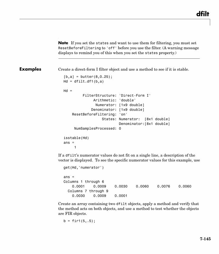
dfilt
Note If you set the states and want to use them for filtering, you must set ResetBeforeFiltering to 'off' before you use the filter. (A warning message displays to remind you of this when you set the states property.)
Examples Create a direct-form I filter object and use a method to see if it is stable.
[b,a] = butter(8,0.25);Hd = dfilt.df1(b,a) Hd = FilterStructure: 'Direct-Form I' Arithmetic: 'double' Numerator: [1x9 double] Denominator: [1x9 double] ResetBeforeFiltering: 'on' States: Numerator: [8x1 double] Denominator:[8x1 double] NumSamplesProcessed: 0
isstable(Hd)ans = 1
If a dfilt’s numerator values do not fit on a single line, a description of the vector is displayed. To see the specific numerator values for this example, use
get(Hd,'numerator')
ans =Columns 1 through 6 0.0001 0.0009 0.0030 0.0060 0.0076 0.0060 Columns 7 through 9 0.0030 0.0009 0.0001
Create an array containing two dfilt objects, apply a method and verify that the method acts on both objects, and use a method to test whether the objects are FIR objects.
b = fir1(5,.5);
7-145
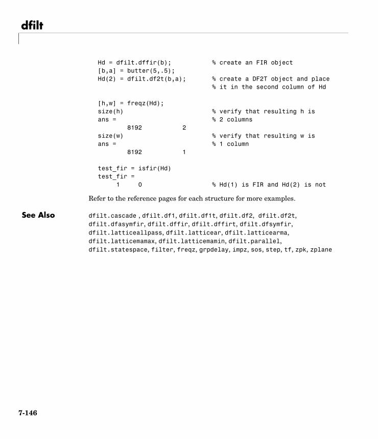
dfilt
Hd = dfilt.dffir(b); % create an FIR object[b,a] = butter(5,.5);Hd(2) = dfilt.df2t(b,a); % create a DF2T object and place
% it in the second column of Hd
[h,w] = freqz(Hd);size(h) % verify that resulting h isans = % 2 columns 8192 2size(w) % verify that resulting w isans = % 1 column 8192 1
test_fir = isfir(Hd)test_fir = 1 0 % Hd(1) is FIR and Hd(2) is not
Refer to the reference pages for each structure for more examples.
See Also dfilt.cascade , dfilt.df1, dfilt.df1t, dfilt.df2, dfilt.df2t, dfilt.dfasymfir, dfilt.dffir, dfilt.dffirt, dfilt.dfsymfir, dfilt.latticeallpass, dfilt.latticear, dfilt.latticearma, dfilt.latticemamax, dfilt.latticemamin, dfilt.parallel, dfilt.statespace, filter, freqz, grpdelay, impz, sos, step, tf, zpk, zplane
7-146
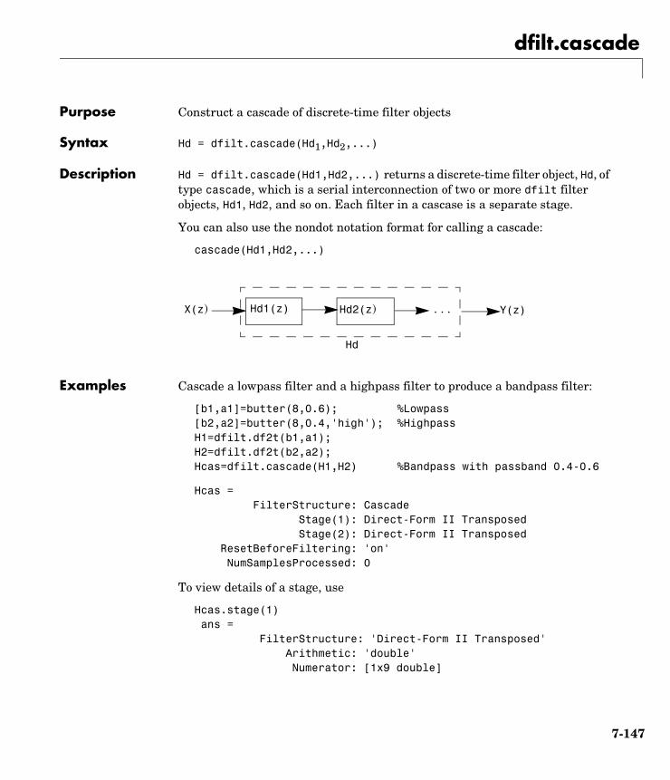
dfilt.cascade
7dfilt.cascadePurpose Construct a cascade of discrete-time filter objects
Syntax Hd = dfilt.cascade(Hd1,Hd2,...)
Description Hd = dfilt.cascade(Hd1,Hd2,...) returns a discrete-time filter object, Hd, of type cascade, which is a serial interconnection of two or more dfilt filter objects, Hd1, Hd2, and so on. Each filter in a cascase is a separate stage.
You can also use the nondot notation format for calling a cascade:
cascade(Hd1,Hd2,...)
Examples Cascade a lowpass filter and a highpass filter to produce a bandpass filter:
[b1,a1]=butter(8,0.6); %Lowpass[b2,a2]=butter(8,0.4,'high'); %HighpassH1=dfilt.df2t(b1,a1);H2=dfilt.df2t(b2,a2);Hcas=dfilt.cascade(H1,H2) %Bandpass with passband 0.4-0.6
Hcas = FilterStructure: Cascade Stage(1): Direct-Form II Transposed Stage(2): Direct-Form II Transposed ResetBeforeFiltering: 'on' NumSamplesProcessed: 0
To view details of a stage, use
Hcas.stage(1) ans = FilterStructure: 'Direct-Form II Transposed' Arithmetic: 'double' Numerator: [1x9 double]
X(z) Y(z)Hd1(z) Hd2(z)
Hd
. . .
7-147

dfilt.cascade
Denominator: [1x9 double] ResetBeforeFiltering: 'on' States: [8x1 double] NumSamplesProcessed: 0
See Also dfilt, dfilt.parallel, dfilt.scalar
7-148
dfilt.df1
7dfilt.df1Purpose Construct a discrete-time, direct-form I filter obImage comparing time and frequency responses of Blackman Hamming Hann and Flattop windowsject
Syntax Hd = dfilt.df1(b,a)Hd = dfilt.df1
Description Hd = dfilt.df1(b,a) returns a discrete-time, direct-form I filter object, Hd, with numerator coefficients b and denominator coefficients a. The filter states for this object are stored in a filtstates object.
Hd = dfilt.df1 returns a default, discrete-time, direct-form I filter object, Hd, with b=1 and a=1. This filter passes the input through to the output unchanged.
Note The leading coefficient of the denominator a(1) cannot be 0.
7-149
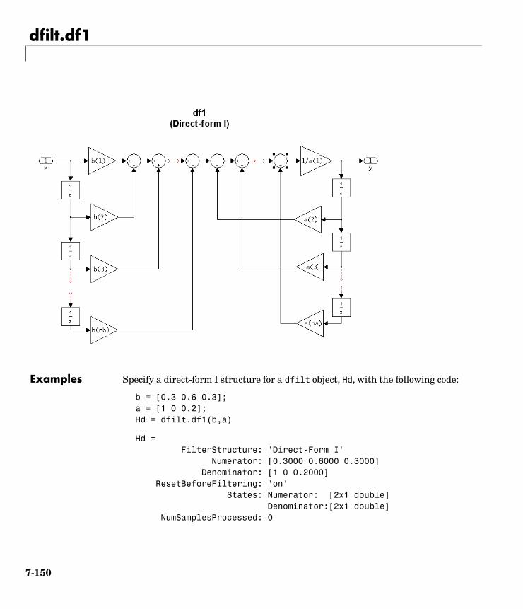
dfilt.df1
Examples Specify a direct-form I structure for a dfilt object, Hd, with the following code:
b = [0.3 0.6 0.3]; a = [1 0 0.2];Hd = dfilt.df1(b,a)
Hd = FilterStructure: 'Direct-Form I' Numerator: [0.3000 0.6000 0.3000] Denominator: [1 0 0.2000] ResetBeforeFiltering: 'on' States: Numerator: [2x1 double] Denominator:[2x1 double] NumSamplesProcessed: 0
7-150

dfilt.df1
See Also dfilt, dfilt.df1t, dfilt.df2, dfilt.df2t
7-151
dfilt.df1sos
7dfilt.df1sosPurpose Construct a discrete-time, second-order section, direct-form I filter object
Syntax Hd = dfilt.df1sos(s)Hd = dfilt.df1sos(b1,a1,b2,a2,...)Hd = dfilt.df1sos(...,g)
Description Hd = dfilt.df1sos(s) returns a discrete-time, second-order section, direct-form I filter object, Hd, with coefficients given in the s matrix. The filter states for this object are stored in a filtstates object.
Hd = dfilt.df1sos(b1,a1,b2,a2,...) returns a discrete-time, second-order section, direct-form I filter object, Hd, with coefficients for the first section given in the b1 and a1 vectors, for the second section given in the b2 and a2 vectors, etc.
Hd = dfilt.df1sos(...,g) includes a gain vector g. The elements of g are the gains for each section. The maximum length of g is the number of sections plus one. If g is not specified, all gains default to one.
Hd = dfilt.df1sos returns a default, discrete-time, second-order section, direct-form I filter object, Hd. This filter passes the input through to the output unchanged.
Note The leading coefficient of the denominator a(1) cannot be 0.
7-152
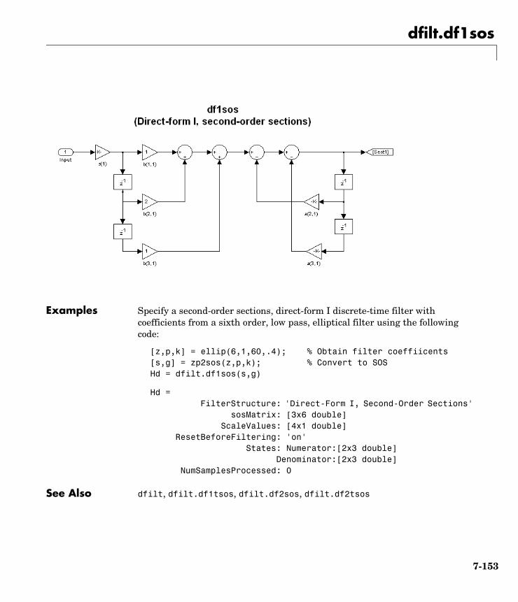
dfilt.df1sos
Examples Specify a second-order sections, direct-form I discrete-time filter with coefficients from a sixth order, low pass, elliptical filter using the following code:
[z,p,k] = ellip(6,1,60,.4); % Obtain filter coeffiicents[s,g] = zp2sos(z,p,k); % Convert to SOSHd = dfilt.df1sos(s,g)
Hd = FilterStructure: 'Direct-Form I, Second-Order Sections' sosMatrix: [3x6 double] ScaleValues: [4x1 double] ResetBeforeFiltering: 'on' States: Numerator:[2x3 double] Denominator:[2x3 double] NumSamplesProcessed: 0
See Also dfilt, dfilt.df1tsos, dfilt.df2sos, dfilt.df2tsos
7-153
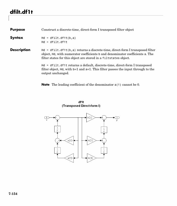
dfilt.df1t
7dfilt.df1tPurpose Construct a discrete-time, direct-form I transposed filter object
Syntax Hd = dfilt.df1t(b,a)Hd = dfilt.df1t
Description Hd = dfilt.df1t(b,a) returns a discrete-time, direct-form I transposed filter object, Hd, with numerator coefficients b and denominator coefficients a. The filter states for this object are stored in a filtstates object.
Hd = dfilt.df1t returns a default, discrete-time, direct-form I transposed filter object, Hd, with b=1 and a=1. This filter passes the input through to the output unchanged.
Note The leading coefficient of the denominator a(1) cannot be 0.
7-154
dfilt.df1t
Examples Specify a direct-form I transposed filter structure for a dfilt object, Hd, with the following code:
b = [0.3 0.6 0.3];a = [1 0 0.2];Hd = dfilt.df1t(b,a)
Hd = FilterStructure: 'Direct-Form I Transposed' Numerator: [0.3000 0.6000 0.3000] Denominator: [1 0 0.2000] ResetBeforeFiltering: 'on' States: Numerator: [2x1 double] Denominator: [2x1 double] NumSamplesProcessed: 0
See Also dfilt, dfilt.df1, dfilt.df2, dfilt.df2t
7-155
dfilt.df1tsos
7dfilt.df1tsosPurpose Construct a discrete-time, second-order section, direct-form I transposed filter object
Syntax Hd = dfilt.df1tsos(s)Hd = dfilt.df1tsos(b1,a1,b2,a2,...)Hd = dfilt.df1tsos(...,g)
Description Hd = dfilt.df1tsos(s) returns a discrete-time, second-order section, direct-form I, transposed filter object, Hd, with coefficients given in the s matrix. The filter states for this object are stored in a filtstates object.
Hd = dfilt.df1tsos(b1,a1,b2,a2,...) returns a discrete-time, second-order section, direct-form I, tranposed filter object, Hd, with coefficients for the first section given in the b1 and a1 vectors, for the second section given in the b2 and a2 vectors, etc.
Hd = dfilt.df1tsos(...,g) includes a gain vector g. The elements of g are the gains for each section. The maximum length of g is the number of sections plus one. If g is not specified, all gains default to one.
Hd = dfilt.df1tsos returns a default, discrete-time, second-order section, direct-form I, transposed filter object, Hd. This filter passes the input through to the output unchanged.
Note The leading coefficient of the denominator a(1) cannot be 0.
7-156
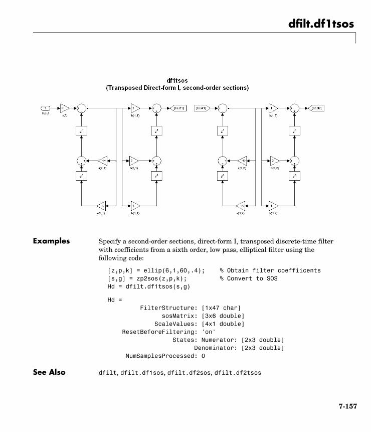
dfilt.df1tsos
Examples Specify a second-order sections, direct-form I, transposed discrete-time filter with coefficients from a sixth order, low pass, elliptical filter using the following code:
[z,p,k] = ellip(6,1,60,.4); % Obtain filter coeffiicents[s,g] = zp2sos(z,p,k); % Convert to SOSHd = dfilt.df1tsos(s,g)
Hd = FilterStructure: [1x47 char] sosMatrix: [3x6 double] ScaleValues: [4x1 double] ResetBeforeFiltering: 'on' States: Numerator: [2x3 double] Denominator: [2x3 double] NumSamplesProcessed: 0
See Also dfilt, dfilt.df1sos, dfilt.df2sos, dfilt.df2tsos
7-157

dfilt.df2
7dfilt.df2Purpose Construct a discrete-time, direct-form II filter object
Syntax Hd = dfilt.df2(b,a)Hd = dfilt.df2
Description Hd = dfilt.df2(b,a) returns a discrete-time, direct-form II filter object, Hd, with numerator coefficients b and denominator coefficients a.
Hd = dfilt.df2 returns a default, discrete-time, direct-form II filter object, Hd, with b=1 and a=1. This filter passes the input through to the output unchanged.
Note The leading coefficient of the denominator a(1) cannot be 0.
7-158
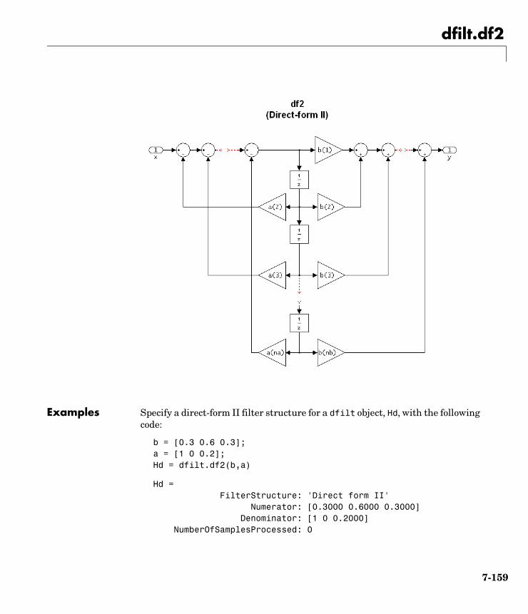
dfilt.df2
Examples Specify a direct-form II filter structure for a dfilt object, Hd, with the following code:
b = [0.3 0.6 0.3];a = [1 0 0.2];Hd = dfilt.df2(b,a)
Hd = FilterStructure: 'Direct form II' Numerator: [0.3000 0.6000 0.3000] Denominator: [1 0 0.2000] NumberOfSamplesProcessed: 0
7-159

dfilt.df2
ResetStates: 'on' States: [2x1 double]
See Also dfilt, dfilt.df1, dfilt.df1t, dfilt.df2t
7-160
dfilt.df2sos
7dfilt.df2sosPurpose Construct a discrete-time, second-order section, direct-form II filter object
Syntax Hd = dfilt.df2sos(s)Hd = dfilt.df2sos(b1,a1,b2,a2,...)Hd = dfilt.df2sos(...,g)
Description Hd = dfilt.df2sos(s) returns a discrete-time, second-order section, direct-form II filter object, Hd, with coefficients given in the s matrix.
Hd = dfilt.df2sos(b1,a1,b2,a2,...) returns a discrete-time, second-order section, direct-form II object, Hd, with coefficients for the first section given in the b1 and a1 vectors, for the second section given in the b2 and a2 vectors, etc.
Hd = dfilt.df2sos(...,g) includes a gain vector g. The elements of g are the gains for each section. The maximum length of g is the number of sections plus one. If g is not specified, all gains default to one.
Hd = dfilt.df2sos returns a default, discrete-time, second-order section, direct-form II filter object, Hd. This filter passes the input through to the output unchanged.
Note The leading coefficient of the denominator a(1) cannot be 0.
7-161
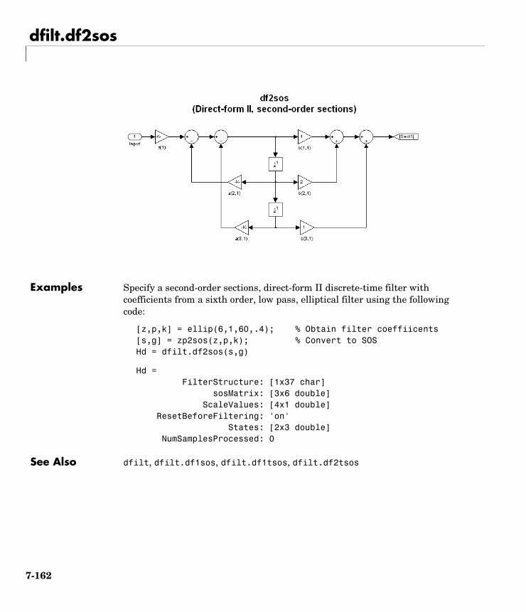
dfilt.df2sos
Examples Specify a second-order sections, direct-form II discrete-time filter with coefficients from a sixth order, low pass, elliptical filter using the following code:
[z,p,k] = ellip(6,1,60,.4); % Obtain filter coeffiicents[s,g] = zp2sos(z,p,k); % Convert to SOSHd = dfilt.df2sos(s,g)
Hd = FilterStructure: [1x37 char] sosMatrix: [3x6 double] ScaleValues: [4x1 double] ResetBeforeFiltering: 'on' States: [2x3 double] NumSamplesProcessed: 0
See Also dfilt, dfilt.df1sos, dfilt.df1tsos, dfilt.df2tsos
7-162
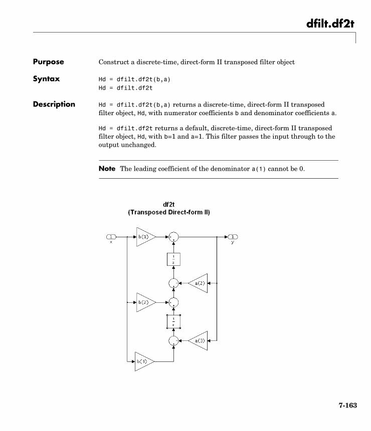
dfilt.df2t
7dfilt.df2tPurpose Construct a discrete-time, direct-form II transposed filter object
Syntax Hd = dfilt.df2t(b,a)Hd = dfilt.df2t
Description Hd = dfilt.df2t(b,a) returns a discrete-time, direct-form II transposed filter object, Hd, with numerator coefficients b and denominator coefficients a.
Hd = dfilt.df2t returns a default, discrete-time, direct-form II transposed filter object, Hd, with b=1 and a=1. This filter passes the input through to the output unchanged.
Note The leading coefficient of the denominator a(1) cannot be 0.
7-163
dfilt.df2t
Examples Specify a second-order direct-form II transposed filter structure for a dfilt object, Hd, with the following code:
b = [0.3 0.6 0.3];a = [1 0 0.2];Hd = dfilt.df2t(b,a)
Hd = FilterStructure: 'Direct form II transposed' Numerator: [0.3000 0.6000 0.3000] Denominator: [1 0 0.2000] NumberOfSamplesProcessed: 0 ResetStates: 'on' States: [2x1 double]
See Also dfilt, dfilt.df1, dfilt.df1t, dfilt.df2
7-164
dfilt.df2tsos
7dfilt.df2tsosPurpose Construct a discrete-time, second-order section, direct-form II transposed filter object
Syntax Hd = dfilt.df2tsos(s)Hd = dfilt.df2tsos(b1,a1,b2,a2,...)Hd = dfilt.df2tsos(...,g)
Description Hd = dfilt.df2sos(s) returns a discrete-time, second-order section, direct-form II, transposed filter object, Hd, with coefficients given in the s matrix.
Hd = dfilt.df2tsos(b1,a1,b2,a2,...) returns a discrete-time, second-order section, direct-form II, tranposed filter object, Hd, with coefficients for the first section given in the b1 and a1 vectors, for the second section given in the b2 and a2 vectors, etc.
Hd = dfilt.df2tsos(...,g) includes a gain vector g. The elements of g are the gains for each section. The maximum length of g is the number of sections plus one. If g is not specified, all gains default to one.
Hd = dfilt.df2tsos returns a default, discrete-time, second-order section, direct-form II, transposed filter object, Hd. This filter passes the input through to the output unchanged.
Note The leading coefficient of the denominator a(1) cannot be 0.
7-165
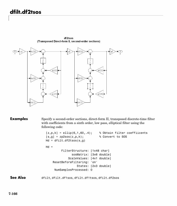
dfilt.df2tsos
Examples Specify a second-order sections, direct-form II, transposed discrete-time filter with coefficients from a sixth order, low pass, elliptical filter using the following code:
[z,p,k] = ellip(6,1,60,.4); % Obtain filter coeffiicents[s,g] = zp2sos(z,p,k); % Convert to SOSHd = dfilt.df2tsos(s,g)
Hd = FilterStructure: [1x48 char] sosMatrix: [3x6 double] ScaleValues: [4x1 double] ResetBeforeFiltering: 'on' States: [2x3 double] NumSamplesProcessed: 0
See Also dfilt, dfilt.df1sos, dfilt.df1tsos, dfilt.df2sos
7-166
dfilt.dfasymfir
7dfilt.dfasymfirPurpose Construct a discrete-time, direct-form antisymmetric FIR filter object
Syntax Hd = dfilt.dfasymfir(b)Hd = dfilt.dfasymfir
Description Hd = dfilt.dfasymfir(b) returns a discrete-time, direct-form, antisymmetric FIR filter object, Hd, with numerator coefficients b.
Hd = dfilt.dfasymfir returns a default, discrete-time, direct-form, antisymmetric FIR filter object, Hd, with b=1. This filter passes the input through to the output unchanged.
Note Only the first half of vector b is used because the second half is assumed to be antisymmetric. In the figure below for an odd number of coefficients, b(3) = 0, b(4) = -b(2) and b(5) = -b(1), and in the next figure for an even number of coefficients, b(4) = -b(3), b(5) = -b(2), and b(6) = -b(1).
7-167
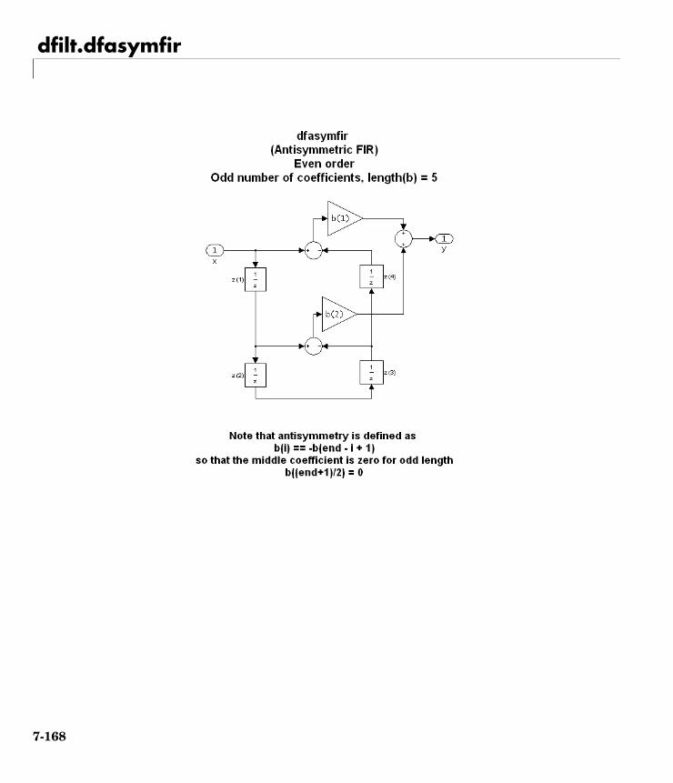
dfilt.dfasymfir
7-168
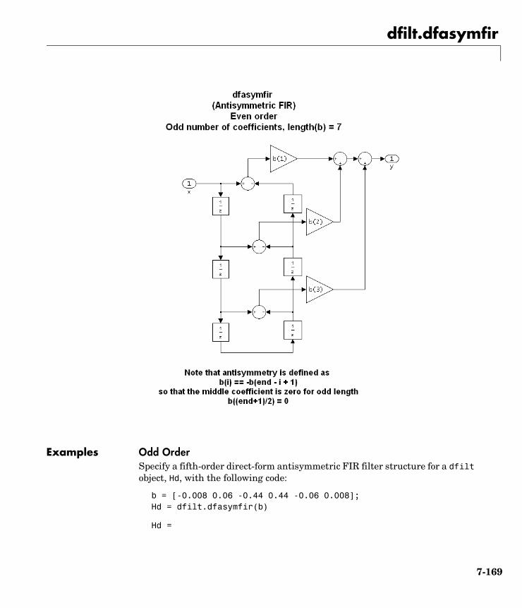
dfilt.dfasymfir
Examples Odd OrderSpecify a fifth-order direct-form antisymmetric FIR filter structure for a dfilt object, Hd, with the following code:
b = [-0.008 0.06 -0.44 0.44 -0.06 0.008];Hd = dfilt.dfasymfir(b)
Hd =
7-169
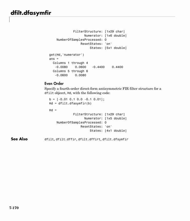
dfilt.dfasymfir
FilterStructure: [1x29 char] Numerator: [1x6 double] NumberOfSamplesProcessed: 0 ResetStates: 'on' States: [5x1 double]
get(Hd,'numerator')ans = Columns 1 through 4 -0.0080 0.0600 -0.4400 0.4400 Columns 5 through 6 -0.0600 0.0080
Even OrderSpecify a fourth-order direct-form antisymmetric FIR filter structure for a dfilt objecct, Hd, with the following code:
b = [-0.01 0.1 0.0 -0.1 0.01];Hd = dfilt.dfasymfir(b)
Hd = FilterStructure: [1x29 char] Numerator: [1x5 double] NumberOfSamplesProcessed: 0 ResetStates: 'on' States: [4x1 double]
See Also dfilt, dfilt.dffir, dfilt.dffirt, dfilt.dfsymfir
7-170
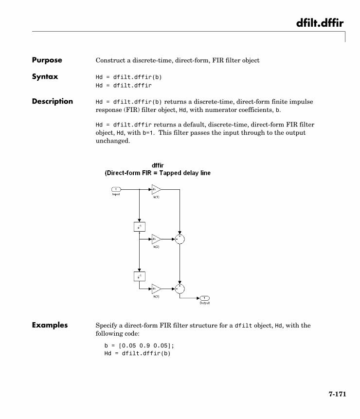
dfilt.dffir
7dfilt.dffirPurpose Construct a discrete-time, direct-form, FIR filter object
Syntax Hd = dfilt.dffir(b)Hd = dfilt.dffir
Description Hd = dfilt.dffir(b) returns a discrete-time, direct-form finite impulse response (FIR) filter object, Hd, with numerator coefficients, b.
Hd = dfilt.dffir returns a default, discrete-time, direct-form FIR filter object, Hd, with b=1. This filter passes the input through to the output unchanged.
Examples Specify a direct-form FIR filter structure for a dfilt object, Hd, with the following code:
b = [0.05 0.9 0.05];Hd = dfilt.dffir(b)
7-171

dfilt.dffir
Hd = FilterStructure: [1x15 char] Numerator: [1x3 double] NumberOfSamplesProcessed: 0 ResetStates: 'on' States: [2x1 double]
See Also dfilt, dfilt.dfasymfir, dfilt.dffirt, dfilt.dfsymfir
7-172
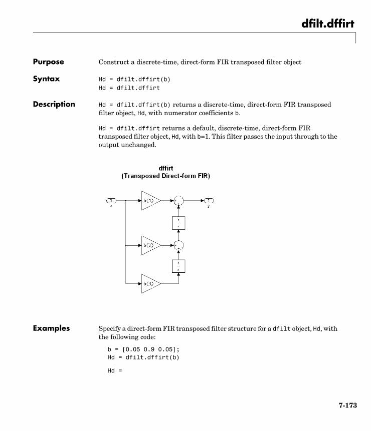
dfilt.dffirt
7dfilt.dffirtPurpose Construct a discrete-time, direct-form FIR transposed filter object
Syntax Hd = dfilt.dffirt(b)Hd = dfilt.dffirt
Description Hd = dfilt.dffirt(b) returns a discrete-time, direct-form FIR transposed filter object, Hd, with numerator coefficients b.
Hd = dfilt.dffirt returns a default, discrete-time, direct-form FIR transposed filter object, Hd, with b=1. This filter passes the input through to the output unchanged.
Examples Specify a direct-form FIR transposed filter structure for a dfilt object, Hd, with the following code:
b = [0.05 0.9 0.05];Hd = dfilt.dffirt(b)
Hd =
7-173

dfilt.dffirt
FilterStructure: [1x26 char] Numerator: [1x3 double] NumberOfSamplesProcessed: 0 ResetStates: 'on' States: [2x1 double]
See Also dfilt, dfilt.dffir, dfilt.dfasymfir, dfilt.dfsymfir
7-174
dfilt.dfsymfir
7dfilt.dfsymfirPurpose Construct a discrete-time, direct-form symmetric FIR filter object
Syntax Hd = dfilt.dfsymfir(b)Hd = dfilt.dfsymfir
Description Hd = dfilt.dfsymfir(b) returns a discrete-time, direct-form symmetric FIR filter object, Hd, with numerator coefficients b.
Hd = dfilt.dfsymfir returns a default, discrete-time, direct-form symmetric FIR filter object, Hd, with b=1. This filter passes the input through to the output unchanged.
Note Only the first half of vector b is used because the second half is assumed to be symmetric. In the figure below for an odd number of coefficients, b(3) = 0, b(4) = b(2) and b(5) = b(1), and in the next figure for an even number of coefficients, b(4) = b(3), b(5) = b(2), and b(6) = b(1).
7-175
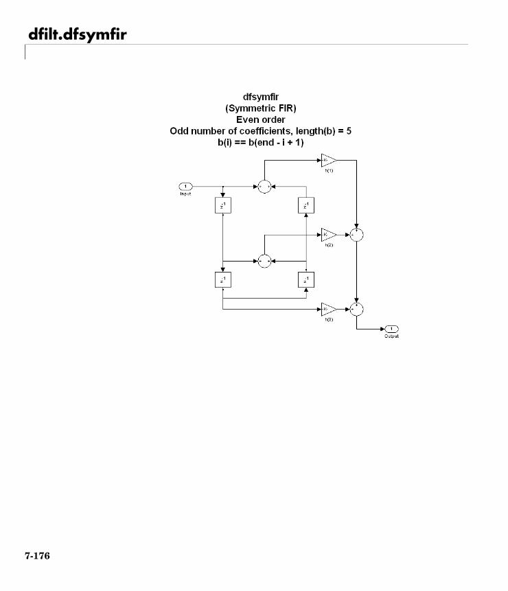
dfilt.dfsymfir
7-176
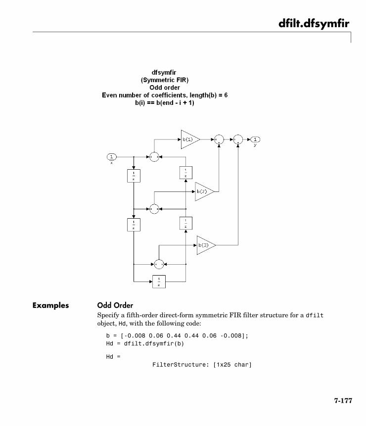
dfilt.dfsymfir
Examples Odd OrderSpecify a fifth-order direct-form symmetric FIR filter structure for a dfilt object, Hd, with the following code:
b = [-0.008 0.06 0.44 0.44 0.06 -0.008];Hd = dfilt.dfsymfir(b)
Hd = FilterStructure: [1x25 char]
7-177
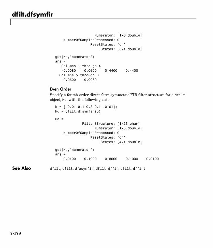
dfilt.dfsymfir
Numerator: [1x6 double] NumberOfSamplesProcessed: 0 ResetStates: 'on' States: [5x1 double]
get(Hd,'numerator')ans = Columns 1 through 4 -0.0080 0.0600 0.4400 0.4400 Columns 5 through 6 0.0600 -0.0080
Even OrderSpecify a fourth-order direct-form symmetric FIR filter structure for a dfilt object, Hd, with the following code:
b = [-0.01 0.1 0.8 0.1 -0.01];Hd = dfilt.dfsymfir(b)
Hd = FilterStructure: [1x25 char] Numerator: [1x5 double] NumberOfSamplesProcessed: 0 ResetStates: 'on' States: [4x1 double]
get(Hd,'numerator')ans = -0.0100 0.1000 0.8000 0.1000 -0.0100
See Also dfilt, dfilt.dfasymfir, dfilt.dffir, dfilt.dffirt
7-178
dfilt.fftfir
7dfilt.fftfirPurpose Construct a discrete-time, overlap-add, FIR filter object
Syntax Hd = dfilt.fftfir(b,len)Hd = dfilt.fftfir(b)Hd = dfilt.fftfir
Description This object uses the overlap-add method of block FIR filtering, which is very efficient for streaming data.
Hd = dfilt.fftfir(b,len) returns a discrete-time, FFT, FIR filter object, Hd, with numerator coefficients, b and block length, len. The block length is the number of input points to use for each overlap-add computation.
Hd = dfilt.fftfir(b) returns a discrete-time, FFT, FIR filter object, Hd, with numerator coefficients, b and block length, len=100.
Hd = dfilt.fftfir returns a default, discrete-time, FFT, FIR filter object, Hd, with the numerator b=1 and block length, len=100. This filter passes the input through to the output unchanged.
Note When you use a dfilt.fftfir object to filter, the input signal length must be an integer multiple of the object’s block length, len.
The resulting number of FFT points = ((filter length + the block length - 1). The filter is most efficient if the number of FFT points is a power of 2.
Examples Specify a second-order, FFT, FIR filter structure for a dfilt object, Hd, with the following code:
b = [0.05 0.9 0.05];len = 50;Hd = dfilt.fftfir(b,len)
Hd = FilterStructure: 'Overlap-Add FIR' Numerator: [0.0500 0.9000 0.0500] BlockLength: 50
7-179

dfilt.fftfir
NonProcessedSamples: [] NumberOfSamplesProcessed: 0 ResetStates: 'on' States: [2x1 double]
To view the frequency domain coefficients used in the filtering, use the following command.
fftcoeffs(Hd)
See Also dfilt, dfilt.dffir, dfilt.dfasymfir, dfilt.dffirt, dfilt.dfsymfir
7-180
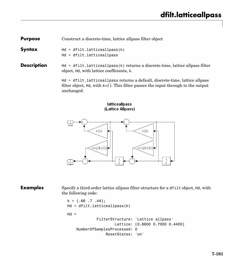
dfilt.latticeallpass
7dfilt.latticeallpassPurpose Construct a discrete-time, lattice allpass filter object
Syntax Hd = dfilt.latticeallpass(k)Hd = dfilt.latticeallpass
Description Hd = dfilt.latticeallpass(k) returns a discrete-time, lattice allpass filter object, Hd, with lattice coefficients, k.
Hd = dfilt.latticeallpass returns a default, discrete-time, lattice allpass filter object, Hd, with k=[ ]. This filter passes the input through to the output unchanged.
Examples Specify a third-order lattice allpass filter structure for a dfilt object, Hd, with the following code:
k = [.66 .7 .44];Hd = dfilt.latticeallpass(k)
Hd = FilterStructure: 'Lattice allpass' Lattice: [0.6600 0.7000 0.4400] NumberOfSamplesProcessed: 0 ResetStates: 'on'
7-181

dfilt.latticeallpass
States: [3x1 double]
See Also dfilt, dfilt.latticear, dfilt.latticearma, dfilt.latticemamax, dfilt.latticemamin
7-182
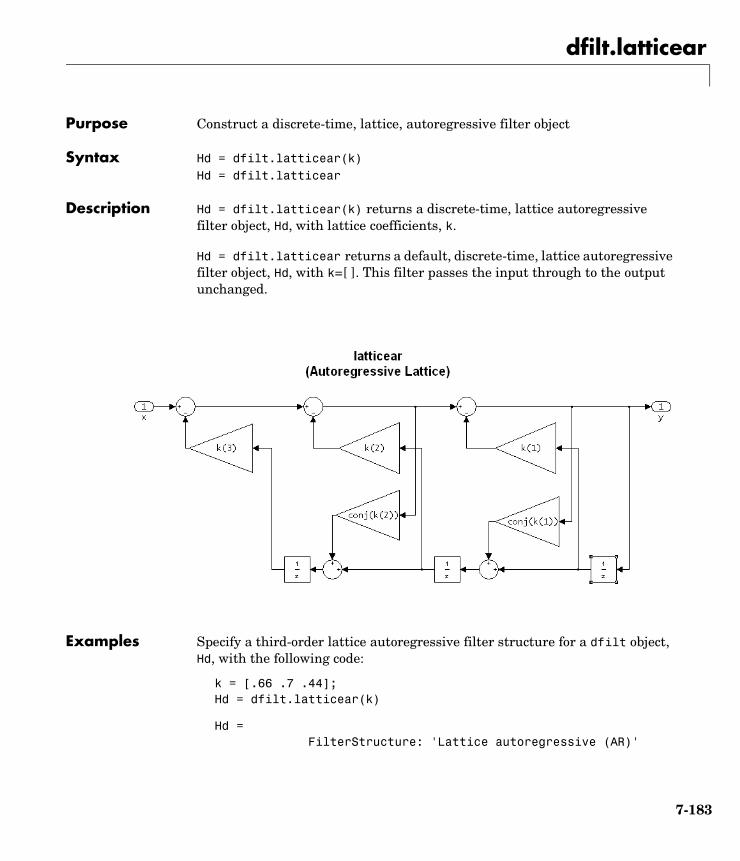
dfilt.latticear
7dfilt.latticearPurpose Construct a discrete-time, lattice, autoregressive filter object
Syntax Hd = dfilt.latticear(k)Hd = dfilt.latticear
Description Hd = dfilt.latticear(k) returns a discrete-time, lattice autoregressive filter object, Hd, with lattice coefficients, k.
Hd = dfilt.latticear returns a default, discrete-time, lattice autoregressive filter object, Hd, with k=[ ]. This filter passes the input through to the output unchanged.
Examples Specify a third-order lattice autoregressive filter structure for a dfilt object, Hd, with the following code:
k = [.66 .7 .44];Hd = dfilt.latticear(k)
Hd = FilterStructure: 'Lattice autoregressive (AR)'
7-183

dfilt.latticear
Lattice: [0.6600 0.7000 0.4400] NumberOfSamplesProcessed: 0 ResetStates: 'on' States: [3x1 double] Lattice: [0.6600 0.7000 0.4400]
See Also dfilt, dfilt.latticeallpass, dfilt.latticearma, dfilt.latticemamax, dfilt.latticemamin
7-184
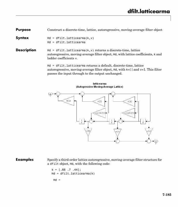
dfilt.latticearma
7dfilt.latticearmaPurpose Construct a discrete-time, lattice, autoregressive, moving-average filter object
Syntax Hd = dfilt.latticearma(k,v)Hd = dfilt.latticearma
Description Hd = dfilt.latticearma(k,v) returns a discrete-time, lattice autoregressive, moving-average filter object, Hd, with lattice coefficients, k and ladder coefficients v.
Hd = dfilt.latticearma returns a default, discrete-time, lattice autoregressive, moving-average filter object, Hd, with k=[ ] and v=1. This filter passes the input through to the output unchanged.
Examples Specify a third-order lattice autoregressive, moving-average filter structure for a dfilt object, Hd, with the following code:
k = [.66 .7 .44];Hd = dfilt.latticearma(k)
Hd =
7-185
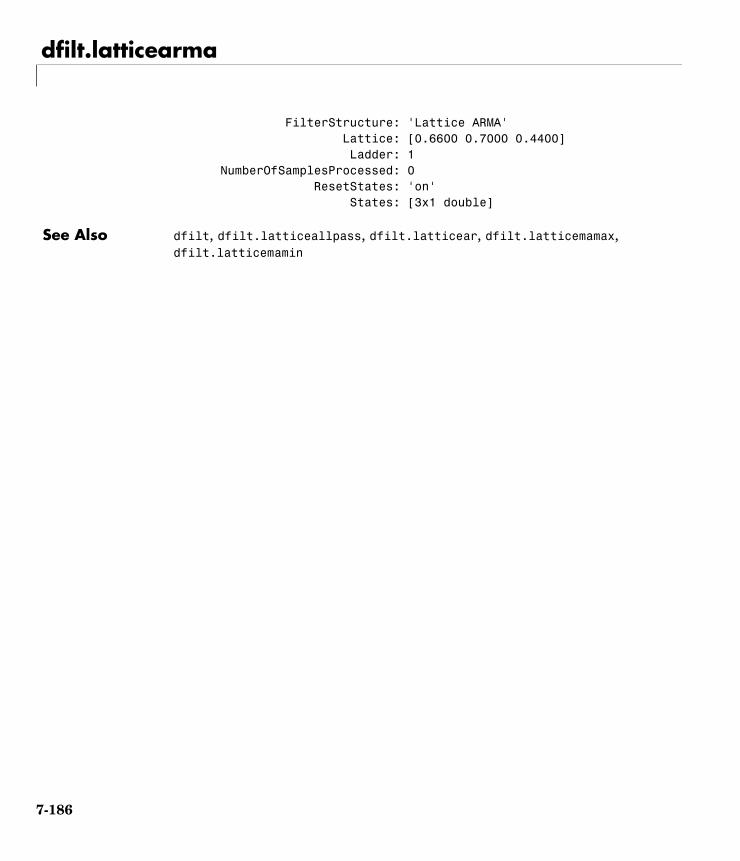
dfilt.latticearma
FilterStructure: 'Lattice ARMA' Lattice: [0.6600 0.7000 0.4400] Ladder: 1 NumberOfSamplesProcessed: 0 ResetStates: 'on' States: [3x1 double]
See Also dfilt, dfilt.latticeallpass, dfilt.latticear, dfilt.latticemamax, dfilt.latticemamin
7-186
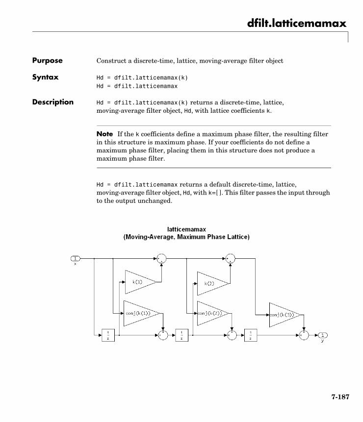
dfilt.latticemamax
7dfilt.latticemamaxPurpose Construct a discrete-time, lattice, moving-average filter object
Syntax Hd = dfilt.latticemamax(k)Hd = dfilt.latticemamax
Description Hd = dfilt.latticemamax(k) returns a discrete-time, lattice, moving-average filter object, Hd, with lattice coefficients k.
Note If the k coefficients define a maximum phase filter, the resulting filter in this structure is maximum phase. If your coefficients do not define a maximum phase filter, placing them in this structure does not produce a maximum phase filter.
Hd = dfilt.latticemamax returns a default discrete-time, lattice, moving-average filter object, Hd, with k=[ ]. This filter passes the input through to the output unchanged.
7-187
dfilt.latticemamax
Examples Specify a fourth-order lattice, moving-average, maximum phase filter structure for a dfilt object, Hd, with the following code:
k = [.66 .7 .44 .33];Hd = dfilt.latticemamax(k)
Hd = FilterStructure: 'Lattice maximum phase' Lattice: [1x4 double] NumberOfSamplesProcessed: 0 ResetStates: 'on' States: [4x1 double]
See Also dfilt, dfilt.latticeallpass, dfilt.latticear, dfilt.latticearma, dfilt.latticemamin
7-188
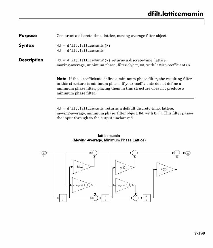
dfilt.latticemamin
7dfilt.latticemaminPurpose Construct a discrete-time, lattice, moving-average filter object
Syntax Hd = dfilt.latticemamin(k)Hd = dfilt.latticemamin
Description Hd = dfilt.latticemamin(k) returns a discrete-time, lattice, moving-average, minimum phase, filter object, Hd, with lattice coefficients k.
Note If the k coefficients define a minimum phase filter, the resulting filter in this structure is minimum phase. If your coefficients do not define a minimum phase filter, placing them in this structure does not produce a minimum phase filter.
Hd = dfilt.latticemamin returns a default discrete-time, lattice, moving-average, minimum phase, filter object, Hd, with k=[ ]. This filter passes the input through to the output unchanged.
7-189
dfilt.latticemamin
Examples Specify a third-order lattice, moving-average, minimup phase, filter structure for a dfilt object, Hd, with the following code:
k = [.66 .7 .44];Hd = dfilt.latticemamin(k)
Hd = FilterStructure: 'Lattice moving-average (MA)' Lattice: [0.6600 0.7000 0.4400] NumberOfSamplesProcessed: 0 ResetStates: 'on' States: [3x1 double]
See Also dfilt, dfilt.latticeallpass, dfilt.latticear, dfilt.latticearma, dfilt.latticemamax
7-190
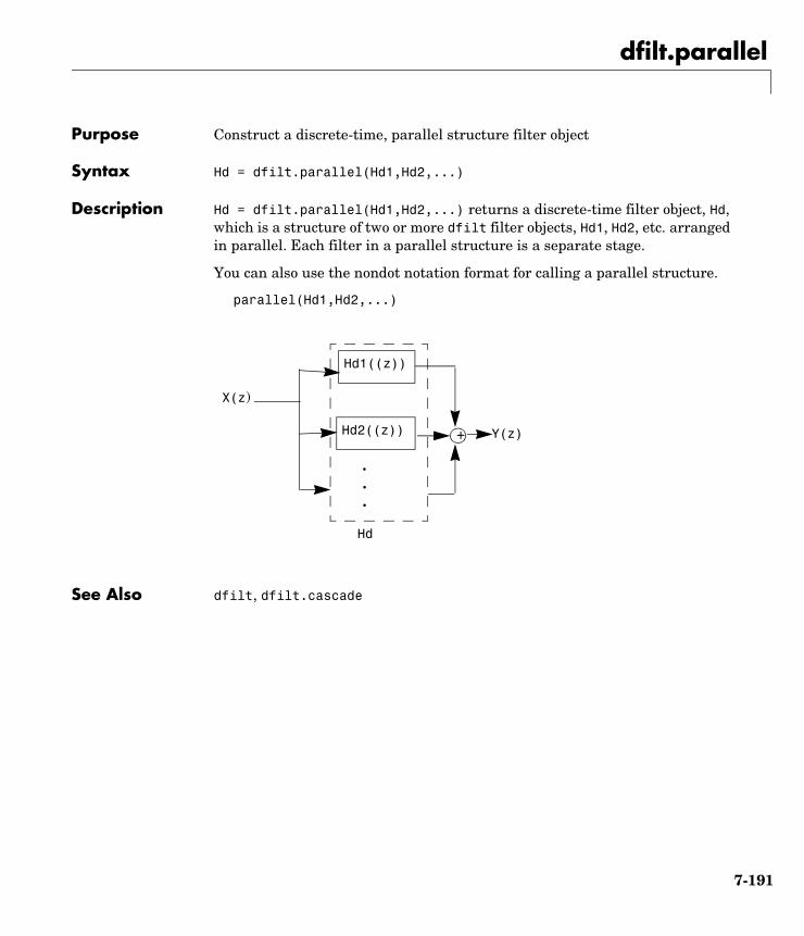
dfilt.parallel
7dfilt.parallelPurpose Construct a discrete-time, parallel structure filter object
Syntax Hd = dfilt.parallel(Hd1,Hd2,...)
Description Hd = dfilt.parallel(Hd1,Hd2,...) returns a discrete-time filter object, Hd, which is a structure of two or more dfilt filter objects, Hd1, Hd2, etc. arranged in parallel. Each filter in a parallel structure is a separate stage.
You can also use the nondot notation format for calling a parallel structure.
parallel(Hd1,Hd2,...)
See Also dfilt, dfilt.cascade
X(z)
Y(z)
Hd1((z))
Hd2((z)) +
Hd
. . .
7-191
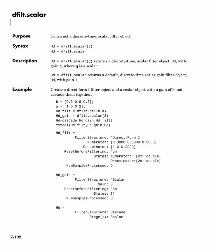
dfilt.scalar
7dfilt.scalarPurpose Construct a discrete-time, scalar filter object
Syntax Hd = dfilt.scalar(g)Hd = dfilt.scalar
Description Hd = dfilt.scalar(g) returns a discrete-time, scalar filter object, Hd, with gain g, where g is a scalar.
Hd = dfilt.scalar returns a default, discrete-time scalar gain filter object, Hd, with gain 1.
Example Create a direct-form I filter object and a scalar object with a gain of 3 and cascade them together.
b = [0.3 0.6 0.3];a = [1 0 0.2];Hd_filt = dfilt.df1(b,a)Hd_gain = dfilt.scalar(3)Hd=cascade(Hd_gain,Hd_filt)fvtool(Hd_filt,Hd_gain,Hd)
Hd_filt = FilterStructure: 'Direct-Form I' Numerator: [0.3000 0.6000 0.3000] Denominator: [1 0 0.2000] ResetBeforeFiltering: 'on' States: Numerator: [2x1 double] Denominator:[2x1 double] NumSamplesProcessed: 0
Hd_gain = FilterStructure: 'Scalar' Gain: 3 ResetBeforeFiltering: 'on' States: [] NumSamplesProcessed: 0
Hd = FilterStructure: Cascade Stage(1): Scalar
7-192
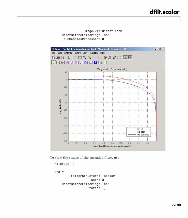
dfilt.scalar
Stage(2): Direct-Form I ResetBeforeFiltering: 'on' NumSamplesProcessed: 0
To view the stages of the cascaded filter, use
Hd.stage(1) ans = FilterStructure: 'Scalar' Gain: 3 ResetBeforeFiltering: 'on' States: []
7-193

dfilt.scalar
NumSamplesProcessed: 0
and
Hd.stage(2) ans = FilterStructure: 'Direct-Form I' Numerator: [1x3 double] Denominator: [1 0 0.2000] ResetBeforeFiltering: 'on' States: Numerator: [2x1 double] Denominator:[2x1 double] NumSamplesProcessed: 0
See Also dfilt, dfilt.cascade
7-194
dfilt.statespace
7dfilt.statespacePurpose Construct a discrete-time, state-space filter object
Syntax Hd = dfilt.statespace(A,B,C,D)Hd = dfilt.statespace
Description Hd = dfilt.statespace(A,B,C,D) returns a discrete-time state-space filter object, Hd, with rectangular arrays A, B, C and D.
A, B, C, and D are from the matrix or state-space form of a filter’s difference equations
where x(n) is the vector states at time n, u(n) is the input at time n, y is the output at time n, A is the state-transition matrix, B is the input-to-state transmission matrix, C is the state-to-output transmission matrix, and D is the input-to-ouput transmission matrix. For single-channel systems, A is an m-by-m matrix where m is the order of the filter, B is a column vector, C is a row vector, and D is a scalar.
Hd = dfilt.statespace returns a default, discrete-time state-space filter object, Hd, with A=[ ], B=[ ], C=[ ], and D=1. This filter passes the input through to the output unchanged.
x n 1+( ) Ax n( ) Bu n( )+=
y n( ) Cx n( ) Du n( )+=
7-195
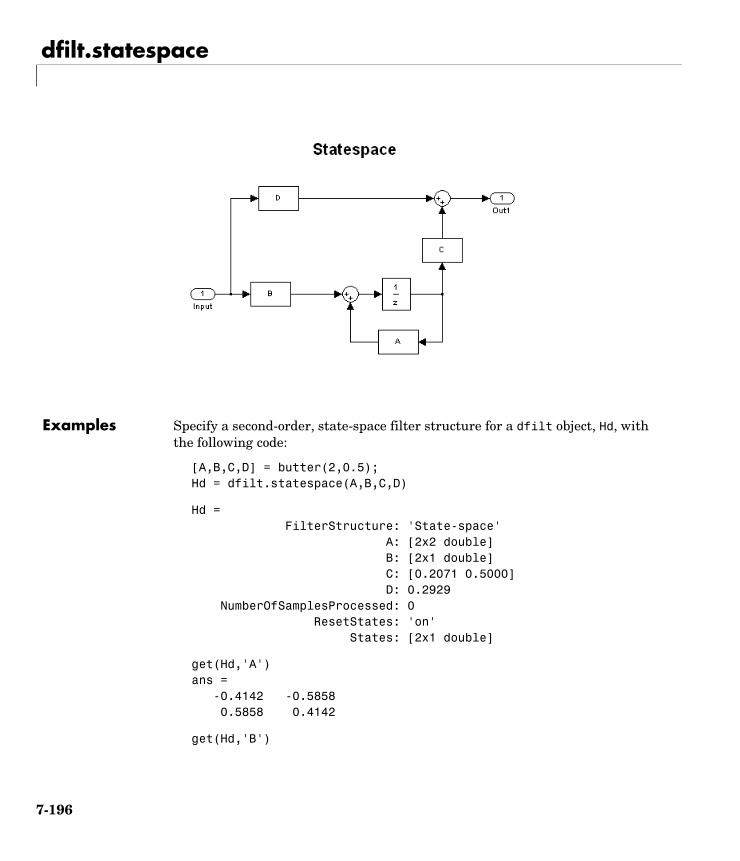
dfilt.statespace
Examples Specify a second-order, state-space filter structure for a dfilt object, Hd, with the following code:
[A,B,C,D] = butter(2,0.5);Hd = dfilt.statespace(A,B,C,D)
Hd = FilterStructure: 'State-space' A: [2x2 double] B: [2x1 double] C: [0.2071 0.5000] D: 0.2929 NumberOfSamplesProcessed: 0 ResetStates: 'on' States: [2x1 double]
get(Hd,'A')ans = -0.4142 -0.5858 0.5858 0.4142
get(Hd,'B')
7-196

dfilt.statespace
ans = 0.8284 0.8284
See Also dfilt
7-197
dftmtx
7dftmtxPurpose Discrete Fourier transform matrix
Syntax A = dftmtx(n)
Description A discrete Fourier transform matrix is a complex matrix of values around the unit circle, whose matrix product with a vector computes the discrete Fourier transform of the vector.
A = dftmtx(n) returns the n-by-n complex matrix A that, when multiplied into a length n column vector x.
y = A*x
computes the discrete Fourier transform of x.
The inverse discrete Fourier transform matrix is
Ai = conj(dftmtx(n))/n
Examples In practice, the discrete Fourier transform is computed more efficiently and uses less memory with an FFT algorithm
x = 1:256;y1 = fft(x);
than by using the Fourier transform matrix.
n = length(x);y2 = x*dftmtx(n);norm(y1-y2)
ans =1.8297e-009
Algorithm dftmtx takes the FFT of the identity matrix to generate the transform matrix.
See Also convmtx, fft
7-198
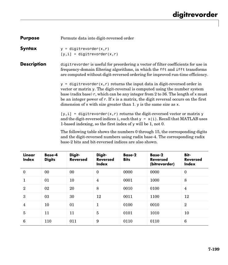
digitrevorder
7digitrevorderPurpose Permute data into digit-reversed order
Syntax y = digitrevorder(x,r)[y,i] = digitrevorder(x,r)
Description digitrevorder is useful for preordering a vector of filter coefficients for use in frequency-domain filtering algorithms, in which the fft and ifft transforms are computed without digit-reversed ordering for improved run-time efficiency.
y = digitrevorder(x,r) returns the input data in digit-reversed order in vector or matrix y. The digit-reversal is computed using the number system base (radix base) r, which can be any integer from 2 to 36. The length of x must be an integer power of r. If x is a matrix, the digit reversal occurs on the first dimension of x with size greater than 1. y is the same size as x.
[y,i] = digitrevorder(x,r) returns the digit-reversed vector or matrix y and the digit-reversed indices i, such that y = x(i). Recall that MATLAB uses 1-based indexing, so the first index of y will be 1, not 0.
The following table shows the numbers 0 through 15, the corresponding digits and the digit-reversed numbers using radix base-4. The corresponding radix base-2 bits and bit-reversed indices are also shown.
Linear Index
Base-4 Digits
Digit-Reversed
Digit-Reversed Index
Base-2 Bits
Base-2 Reversed (bitrevorder)
Bit-Reversed Index
0 00 00 0 0000 0000 0
1 01 10 4 0001 1000 8
2 02 20 8 0010 0100 4
3 03 30 12 0011 1100 12
4 10 01 1 0100 0010 2
5 11 11 5 0101 1010 10
6 110 011 9 0110 0110 6
7-199

digitrevorder
Examples Obtain the digit-reversed, radix base-3 ordered output of a vector containing 9 values:
x=[0:8]'; % Create a column vector[x,digitrevorder(x,3)]ans =
0 0 1 3 2 6 3 1 4 4 5 7 6 2 7 5 8 8
See Also bitrevorder, fft, ifft
7 13 31 13 0111 1110 14
8 20 02 2 1000 0001 1
9 21 12 6 1001 1001 9
10 22 22 10 1010 0101 5
11 23 32 14 1011 1101 13
12 30 03 3 1100 0011 3
13 31 13 7 1101 1011 11
14 32 23 11 1110 0111 7
15 33 33 15 1111 1111 15
Linear Index
Base-4 Digits
Digit-Reversed
Digit-Reversed Index
Base-2 Bits
Base-2 Reversed (bitrevorder)
Bit-Reversed Index
7-200
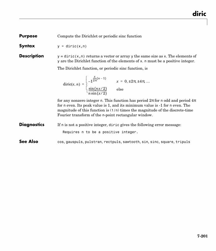
diric
7diricPurpose Compute the Dirichlet or periodic sinc function
Syntax y = diric(x,n)
Description y = diric(x,n) returns a vector or array y the same size as x. The elements of y are the Dirichlet function of the elements of x. n must be a positive integer.
The Dirichlet function, or periodic sinc function, is
for any nonzero integer n. This function has period 2π for n odd and period 4π for n even. Its peak value is 1, and its minimum value is -1 for n even. The magnitude of this function is (1/n) times the magnitude of the discrete-time Fourier transform of the n-point rectangular window.
Diagnostics If n is not a positive integer, diric gives the following error message:
Requires n to be a positive integer.
See Also cos, gauspuls, pulstran, rectpuls, sawtooth, sin, sinc, square, tripuls
diric x n,( )1–
x2π------- n 1–( )
x 0 2π± 4π± …, , ,=
nx 2⁄( )sinn x 2⁄( )sin---------------------------- else
=
7-201
downsample
7downsamplePurpose Decrease the sampling rate of the input signal
Syntax y = downsample(x,n)y = downsample(x,n,phase)
Description y = downsample(x,n) decreases the sampling rate of x by keeping every nth sample starting with the first sample. x can be a vector or a matrix. If x is a matrix, each column is considered a separate sequence.
y = downsample(x,n,phase) specifies the number of samples by which to offset the downsampled sequence. phase must be an integer from 0 to n-1.
Examples Decrease the sampling rate of a sequence by 3:
x = [1 2 3 4 5 6 7 8 9 10];y = downsample(x,3)
y =1 4 7 10
Decrease the sampling rate of the sequence by 3 and add a phase offset of 2:
y = downsample(x,3,2)
y =3 6 9
Decrease the sampling rate of a matrix by 3:
x = [1 2 3; 4 5 6; 7 8 9; 10 11 12];y = downsample(x,3);x,y
x =1 2 34 5 67 8 910 11 12
y = 1 2 310 11 12
7-202

downsample
See Also decimate, interp, interp1, resample, spline, upfirdn, upsample
7-203
dpss
7dpssPurpose Discrete prolate spheroidal sequences (Slepian sequences)
Syntax [e,v] = dpss(n,nw)[e,v] = dpss(n,nw,k)[e,v] = dpss(n,nw,[k1 k2])[e,v] = dpss(n,nw,'int')[e,v] = dpss(n,nw,'int',Ni)[e,v] = dpss(...,'trace')
Description [e,v] = dpss(n,nw) generates the first 2*nw discrete prolate spheroidal sequences (DPSS) of length n in the columns of e, and their corresponding concentrations in vector v. They are also generated in the DPSS MAT-file database dpss.mat. nw must be less than n/2.
[e,v] = dpss(n,nw,k) returns the k most band-limited discrete prolate spheroidal sequences. k must be an integer such that 1 ≤ k ≤ n.
[e,v] = dpss(n,nw,[k1 k2]) returns the k1st through the k2nd discrete prolate spheroidal sequences, where 1 ≤ k1 ≤ k2 ≤ n.
For all of the above forms:
• The Slepian sequences are calculated directly.
• The sequences are generated in the frequency band |ω| ≤ (2πW), where W = nw/n is the half-bandwidth and ω is in rad/sample.
• e(:,1) is the length n signal most concentrated in the frequency band |ω| ≤ (2πW) radians, e(:,2) is the signal orthogonal to e(:,1) that is most concentrated in this band, e(:,3) is the signal orthogonal to both e(:,1) and e(:,2) that is most concentrated in this band, etc.
• For multitaper spectral analysis, typical choices for nw are 2, 5/2, 3, 7/2, or 4.
[e,v] = dpss(n,nw,'int') uses the interpolation method specified by the string 'int' to compute e and v from the sequences in dpss.mat with length closest to n. The string 'int' can be either:
• 'spline': Use spline interpolation.
• 'linear': Use linear interpolation. This is much faster but less accurate than spline interpolation.
7-204
dpss
[e,v] = dpss(n,nw,'int',Ni) interpolates from existing length Ni sequences. The interpolation method 'linear' requires Ni > n.
[e,v] = dpss(...,'trace') uses the trailing string 'trace' to display which interpolation method DPSS uses. If you don’t specify the interpolation method, the display indicates that you are using the direct method.
Examples Example 1: Using dpss, dpssave, and dpssdirCreate a catalogue of 16 DPSS functions with nw = 4, and use spline interpolation on 10 of these functions while displaying the interpolation method you use. You can do this using dpss, dpsssave, and dpssdir:
% Create the catalogue of functions.[e,v] = dpss(16,4);
% Save e and v in a MAT-file. dpsssave(4,e,v);
% Find nw = 4. First create a structure called index.index = dpssdir;index.wlistsans = NW: 4 key: 1
% Use spline interpolation on 10 of the DPSS functions.[e1,v1] = dpss(10,4,'spline',size(e,1),'trace');
Example 2: Using dpss and dpssloadCreate a set of DPSS functions using dpss, and use the spline method on a subset of these functions. Use dpssload to load the MAT-file created by dpss:
% Create the catalogue of functions.[e,v] = dpss(16,4);
% Load dpss.mat, where e and v are saved. [e1,v1] = dpssload(16,4);
% Use spline interpolation on 10 of the DPSS functions.[e1,v1] = dpss(10,4,'spline');
See Also dpssclear, dpssdir, dpssload, dpsssave, pmtm
7-205

dpss
References [1] Percival, D.B., and A.T. Walden. Spectral Analysis for Physical Applications: Multitaper and Conventional Univariate Techniques. Cambridge: Cambridge University Press, 1993.
7-206

dpssclear
7dpssclearPurpose Remove discrete prolate spheroidal sequences from database
Syntax dpssclear(n,nw)
Description dpssclear(n,nw) removes sequences with length n and time-bandwidth product nw from the DPSS MAT-file database dpss.mat.
See Also dpss, dpssdir, dpssload, dpsssave
7-207
dpssdir
7dpssdirPurpose Discrete prolate spheroidal sequences database directory
Syntax dpssdirdpssdir(n)dpssdir(nw,'nw')dpssdir(n,nw)index = dpssdir
Description dpssdir manages the database directory that contains the generated DPSS samples in the DPSS MAT-file database dpss.mat.
dpssdir lists the directory of saved sequences in dpss.mat.
dpssdir(n) lists the sequences saved with length n.
dpssdir(nw,'nw') lists the sequences saved with time-bandwidth product nw.
dpssdir(n,nw) lists the sequences saved with length n and time-bandwidth product nw.
index = dpssdir is a structure array describing the DPSS database. Pass n and nw options as for the no output case to get a filtered index.
Examples See “Example 1: Using dpss, dpssave, and dpssdir” on page 7-205.
See Also dpss, dpssclear, dpssload, dpsssave
7-208
dpssload
7dpssloadPurpose Load discrete prolate spheroidal sequences from database
Syntax [e,v] = dpssload(n,nw)
Description [e,v] = dpssload(n,nw) loads all sequences with length n and time-bandwidth product nw in the columns of e and their corresponding concentrations in vector v from the DPSS MAT-file database dpss.mat.
Examples See “Example 2: Using dpss and dpssload” on page 7-205.
See Also dpss, dpssclear, dpssdir, dpsssave
7-209
dpsssave
7dpsssavePurpose Save discrete prolate spheroidal sequences in database
Syntax dpsssave(nw,e,v)status = dpsssave(nw,e,v)
Description dpsssave(nw,e,v) saves the sequences in the columns of e and their corresponding concentrations in vector v in the DPSS MAT-file database dpss.mat. It is not necessary to specify sequence length, because the length of the sequence is determined by the number of rows of e.
nw is the time-bandwidth product that was specified when the sequence was created using dpss.
status = dpsssave(nw,e,v) returns 0 if the save was successful and 1 if there was an error.
Examples See “Example 1: Using dpss, dpssave, and dpssdir” on page 7-205.
See Also dpss, dpssclear, dpssdir, dpssload
7-210
dspdata
7dspdataPurpose DSP data objects
Syntax Hs = dspdata.databoj(input1,...)
Description Hs = dspdata.dataobj(input1,...) returns a dspdata object Hs of type dataobj. This object contains all the parameter information needed for the specified type of dataobj. Each dataobj takes one or more inputs, which are described on the individual reference pages. If you do not specify any input values, the returned object has default property values appropriate for the particular dataobj type.
Note You must use a dataobj with dspdata.
Data ObjectsA data object (dataobj) for dspdata specifies the type of data stored in the object. Available dataobj types for dspdata are shown below.
For more information on each dataobj type, refer to its reference page.
MethodsMethods provide ways of performing functions directly on your dspdata object. You can apply these methods directly on the variable you assigned to your dspdata object.
dspdata.dataobj Description
dspdata.msspectrum Mean-square spectrum data (power)
dspdata.psd Power spectral density data (power/frequency)
dspdata.pseudospectrum Pseudospectrum data (power)
7-211
dspdata
.
Method Description
avgpower Note that this method applies only to dspdata.psd objects.
avgpower(Hs) computes the average power in a given frequency band. The technique uses a rectangle approximation of the integral of the Hs signal’s power spectral density (PSD). If the signal is a matrix, the computation is done on each column. The average power is the total signal power and the SpectrumType property determines whether the total average power is contained in the one-sided or two-sided spectrum. For aa one-sided spectrum, the range is [0,pi] for even number of frequency points and [0,pi) for odd. For a two-sided spectrum the range is [0,2pi).
avgpower(Hs,freqrange) specifies the frequency range over which to calculate the average power. freqrange is a two-element vector of the frequencies between which to calculate. If a frequency value does not match exactly the frequency in Hs, the next closest value is used. Note that the first frequency value in freqrange is included in the calculation and the second value is excluded.
centerdc centerdc(Hs) or centerdc(Hs,true) shifts the data and frequency values so that the DC component is at the center of the spectrum. If the SpectrumType property is 'onesided', it is changed to 'twosided' and then the DC component is centered.
centerdc(Hs,'false') shifts the data and frequency values so that the DC component is at the left edge of the spectrum.
7-212
dspdata
halfrange halfrange(Hs) converts the Hs spectrum to a spectrum calculated over half the Nyquist interval. All associated properties affected by the new frequency range are adjusted automatically. This method is used for dspdata.pseudospectrum objects.
Note that the spectrum is assumed to be from a real signal (that is, halfrange uses half the data points regardless of whether the data is symmetric).
normalizefreq normalizefreq(Hs) or normalizefreq(Hs,true) normalizes the frequency specifications in the Hs object to Fs so the frequencies are between 0 and 1. It also sets the NormalizedFrequency property to true.
normalizefreq(Hs,false) converts the frequencies to linear frequencies.
normalizefreq(Hs,false,Fs) sets a new sampling frequency Fs. This can be used only with false.
onesided onesided(Hs) converts the Hs spectrum to a spectrum calculated over half the Nyquist interval and containing the total signal power. All associated properties affected by the new frequency range are adjusted automatically. This method is used for dspdata.psd and dspdata.msspectrum objects.
Note that the spectrum is assumed to be from a real signal (that is, onesided uses half the data points regardless of whether the data is symmetric).
plot Displays the data graphically in a figure window.
Method Description
7-213
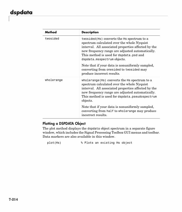
dspdata
Plotting a DSPDATA ObjectThe plot method displays the dspdata object spectrum in a separate figure window, which includes the Signal Processing Toolbox GUI menus and toolbar. Data markers are also available in this window.
plot(Hs) % Plots an existing Hs object
twosided twosided(Hs) converts the Hs spectrum to a spectrum calculated over the whole Nyquist interval. All associated properties affected by the new frequency range are adjusted automatically. This method is used for dspdata.psd and dspdata.msspectrum objects.
Note that if your data is nonuniformly sampled, converting from onesided to twosided may produce incorrect results.
wholerange wholerange(Hs) converts the Hs spectrum to a spectrum calculated over the whole Nyquist interval. All associated properties affected by the new frequency range are adjusted automatically. This method is used for dspdata.pseudospectrum objects.
Note that if your data is nonuniformly sampled, converting from half to wholerange may produce incorrect results.
Method Description
7-214
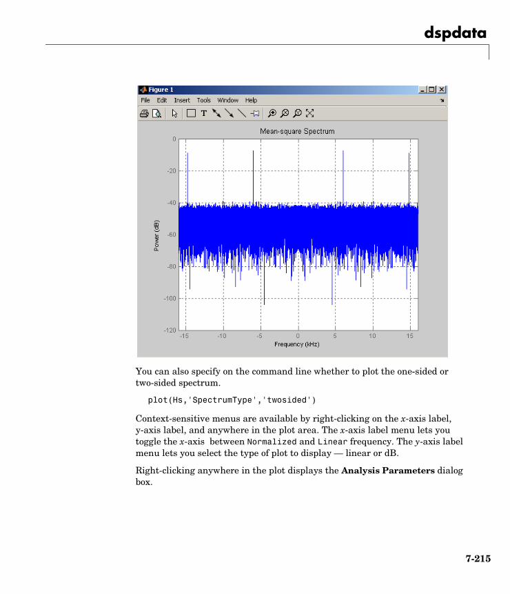
dspdata
You can also specify on the command line whether to plot the one-sided or two-sided spectrum.
plot(Hs,'SpectrumType','twosided')
Context-sensitive menus are available by right-clicking on the x-axis label, y-axis label, and anywhere in the plot area. The x-axis label menu lets you toggle the x-axis between Normalized and Linear frequency. The y-axis label menu lets you select the type of plot to display — linear or dB.
Right-clicking anywhere in the plot displays the Analysis Parameters dialog box.
7-215
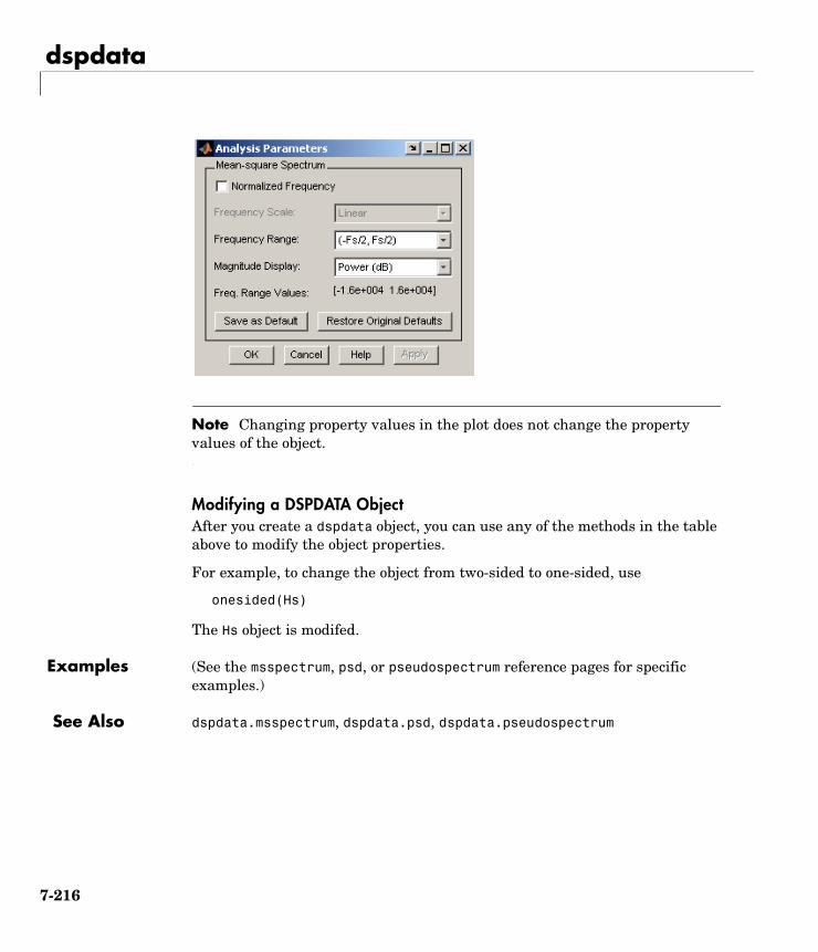
dspdata
Note Changing property values in the plot does not change the property values of the object.
Modifying a DSPDATA ObjectAfter you create a dspdata object, you can use any of the methods in the table above to modify the object properties.
For example, to change the object from two-sided to one-sided, use
onesided(Hs)
The Hs object is modifed.
Examples (See the msspectrum, psd, or pseudospectrum reference pages for specific examples.)
See Also dspdata.msspectrum, dspdata.psd, dspdata.pseudospectrum
7-216
dspdata.msspectrum
7dspdata.msspectrumPurpose Create a mean-square (power) spectrum dspdata object
Syntax Hmss = dspdata.msspectrum(Data)Hmss = dspdata.msspectrum(Data,Frequencies)Hmss = dspdata.msspectrum(...,'Fs',Fs)Hmss = dspdata.msspectrum(...,'SpectrumType',SpectrumType)Hmss = dspdata.msspectrum(...,'CenterDC',flag)
Description The mean-squared spectrum (MSS) is intended for discrete spectra. Unlike the power spectral density (PSD), the peaks in the MSS reflect the power in the signal at a given frequency. The MSS of a signal is the Fourier transform of that signal’s autocorrelation.
Hmss = dspdata.msspectrum(Data) uses the mean-square (power) spectrum data contained in Data, which can be in the form of a vector or a matrix, where each column is a separate set of data. Default values for other properties of the object are as follows:
7-217
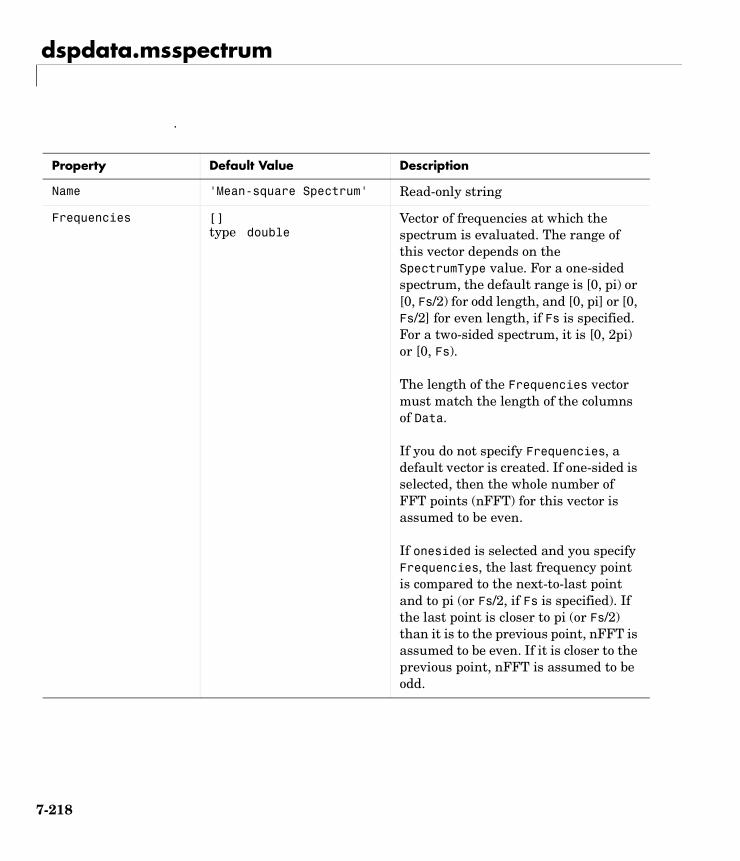
dspdata.msspectrum
.
Property Default Value Description
Name 'Mean-square Spectrum' Read-only string
Frequencies []type double
Vector of frequencies at which the spectrum is evaluated. The range of this vector depends on the SpectrumType value. For a one-sided spectrum, the default range is [0, pi) or [0, Fs/2) for odd length, and [0, pi] or [0, Fs/2] for even length, if Fs is specified. For a two-sided spectrum, it is [0, 2pi) or [0, Fs).
The length of the Frequencies vector must match the length of the columns of Data.
If you do not specify Frequencies, a default vector is created. If one-sided is selected, then the whole number of FFT points (nFFT) for this vector is assumed to be even.
If onesided is selected and you specify Frequencies, the last frequency point is compared to the next-to-last point and to pi (or Fs/2, if Fs is specified). If the last point is closer to pi (or Fs/2) than it is to the previous point, nFFT is assumed to be even. If it is closer to the previous point, nFFT is assumed to be odd.
7-218
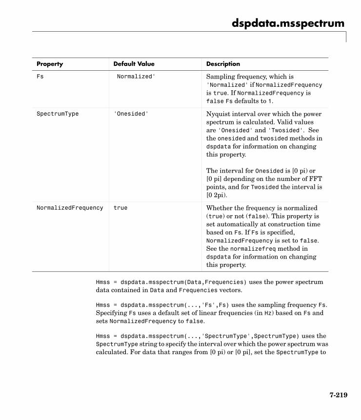
dspdata.msspectrum
Hmss = dspdata.msspectrum(Data,Frequencies) uses the power spectrum data contained in Data and Frequencies vectors.
Hmss = dspdata.msspectrum(...,'Fs',Fs) uses the sampling frequency Fs. Specifying Fs uses a default set of linear frequencies (in Hz) based on Fs and sets NormalizedFrequency to false.
Hmss = dspdata.msspectrum(...,'SpectrumType',SpectrumType) uses the SpectrumType string to specify the interval over which the power spectrum was calculated. For data that ranges from [0 pi) or [0 pi], set the SpectrumType to
Fs Normalized' Sampling frequency, which is 'Normalized' if NormalizedFrequency is true. If NormalizedFrequency is false Fs defaults to 1.
SpectrumType 'Onesided' Nyquist interval over which the power spectrum is calculated. Valid values are 'Onesided' and 'Twosided'. See the onesided and twosided methods in dspdata for information on changing this property.
The interval for Onesided is [0 pi) or [0 pi] depending on the number of FFT points, and for Twosided the interval is [0 2pi).
NormalizedFrequency true Whether the frequency is normalized (true) or not (false). This property is set automatically at construction time based on Fs. If Fs is specified, NormalizedFrequency is set to false. See the normalizefreq method in dspdata for information on changing this property.
Property Default Value Description
7-219
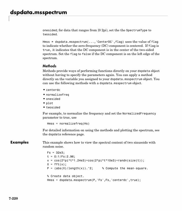
dspdata.msspectrum
onesided; for data that ranges from [0 2pi), set the the SpectrumType to twosided.
Hmss = dspdata.msspectrum(...,'CenterDC',flag) uses the value of flag to indicate whether the zero-frequency (DC) component is centered. If flag is true, it indicates that the DC component is in the center of the two-sided spectrum. Set the flag to false if the DC component is on the left edge of the spectrum.
MethodsMethods provide ways of performing functions directly on your dspdata object without having to specify the parameters again. You can apply a method directly on the variable you assigned to your dspdata.msspectrum object. You can use the following methods with a dspdata.msspectrum object.
• centerdc
• normalizefreq• onesided• plot• twosided
For example, to normalize the frequency and set the NormalizedFrequency parameter to true, use
Hmss = normalizefreq(Hs)
For detailed information on using the methods and plotting the spectrum, see the dspdata reference page.
Examples This example shows how to view the spectral content of two sinusoids with random noise.
Fs = 32e3;t = 0:1/Fs:2.96;x = cos(2*pi*t*1.24e3)+cos(2*pi*t*10e3)+randn(size(t));X = fft(x);P = (abs(X)/length(x)).^2; % Compute the mean-square.
% Create data object.Hmss = dspdata.msspectrum(P,'Fs',Fs,'centerdc',true);
7-220
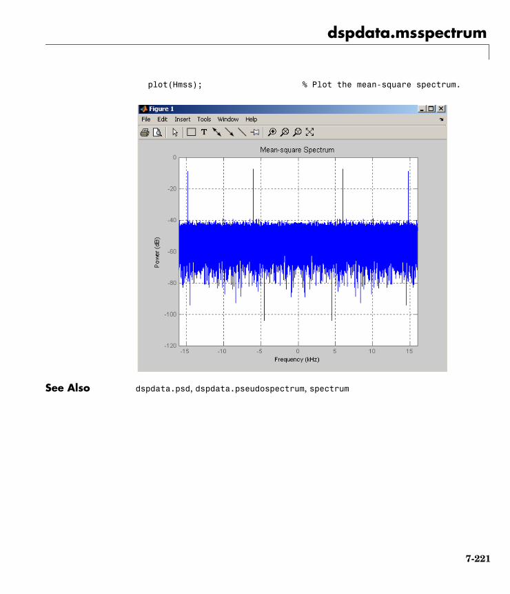
dspdata.msspectrum
plot(Hmss); % Plot the mean-square spectrum.
See Also dspdata.psd, dspdata.pseudospectrum, spectrum
7-221
dspdata.psd
7dspdata.psdPurpose Create a power spectral density dspdata object
Syntax Hpsd = dspdata.psd(Data)Hpsd = dspdata.psd(Data,Frequencies)Hpsd = dspdata.psd(...,'Fs',Fs)Hpsd = dspdata.psd(...,'SpectrumType',SpectrumType)Hpsd = dspdata.psd(...,'CenterDC',flag)
Description The power spectral density (PSD) is intended for continuous spectra. The integral of the PSD over a given frequency band computes the average power in the signal over that frequency band. In contrast to the mean-squared spectrum, the peaks in this spectra do not reflect the power at a given frequency. See the avgpower method of dspdata for more information.
A one-sided PSD contains the total power of the signal in the frequency interval from DC to half of the Nyquist rate. A two-sided PSD contains the total power in the frequency interval from DC to the Nyquist rate.
Hpsd = dspdata.psd(Data) uses the power spectral density data contained in Data, which can be in the form of a vector or a matrix, where each column is a separate set of data. Default values for other properties of the object are shown below:
7-222
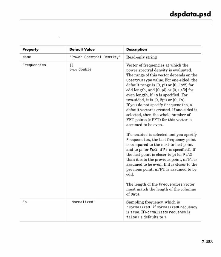
dspdata.psd
.
Property Default Value Description
Name 'Power Spectral Density' Read-only string
Frequencies []type double
Vector of frequencies at which the power spectral density is evaluated. The range of this vector depends on the SpectrumType value. For one-sided, the default range is [0, pi) or [0, Fs/2) for odd length, and [0, pi] or [0, Fs/2] for even length, if Fs is specified. For two-sided, it is [0, 2pi) or [0, Fs).If you do not specify Frequencies, a default vector is created. If one-sided is selected, then the whole number of FFT points (nFFT) for this vector is assumed to be even.
If onesided is selected and you specify Frequencies, the last frequency point is compared to the next-to-last point and to pi (or Fs/2, if Fs is specified). If the last point is closer to pi (or Fs/2) than it is to the previous point, nFFT is assumed to be even. If it is closer to the previous point, nFFT is assumed to be odd.
The length of the Frequencies vector must match the length of the columns of Data.
Fs Normalized' Sampling frequency, which is 'Normalized' if NormalizedFrequency is true. If NormalizedFrequency is false Fs defaults to 1.
7-223
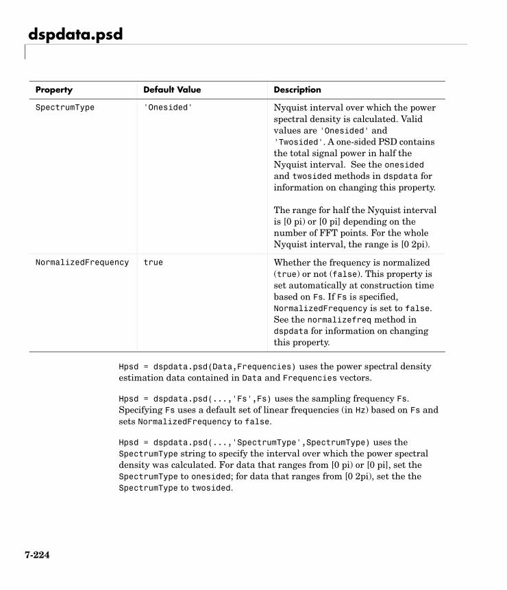
dspdata.psd
Hpsd = dspdata.psd(Data,Frequencies) uses the power spectral density estimation data contained in Data and Frequencies vectors.
Hpsd = dspdata.psd(...,'Fs',Fs) uses the sampling frequency Fs. Specifying Fs uses a default set of linear frequencies (in Hz) based on Fs and sets NormalizedFrequency to false.
Hpsd = dspdata.psd(...,'SpectrumType',SpectrumType) uses the SpectrumType string to specify the interval over which the power spectral density was calculated. For data that ranges from [0 pi) or [0 pi], set the SpectrumType to onesided; for data that ranges from [0 2pi), set the the SpectrumType to twosided.
SpectrumType 'Onesided' Nyquist interval over which the power spectral density is calculated. Valid values are 'Onesided' and 'Twosided'. A one-sided PSD contains the total signal power in half the Nyquist interval. See the onesided and twosided methods in dspdata for information on changing this property.
The range for half the Nyquist interval is [0 pi) or [0 pi] depending on the number of FFT points. For the whole Nyquist interval, the range is [0 2pi).
NormalizedFrequency true Whether the frequency is normalized (true) or not (false). This property is set automatically at construction time based on Fs. If Fs is specified, NormalizedFrequency is set to false. See the normalizefreq method in dspdata for information on changing this property.
Property Default Value Description
7-224
dspdata.psd
Hpsd = dspdata.psd(...,'CenterDC',flag) uses the value of flag to indicate whether the zero-frequency (DC) component is centered. If flag is true, it indicates that the DC component is in the center of the two-sided spectrum. Set the flag to false if the DC component is on the left edge of the spectrum.
MethodsMethods provide ways of performing functions directly on your dspdata object. You can apply a method directly on the variable you assigned to your dspdata.psd object. You can use the following methods with a dspdata.psd object.
• avgpower• centerdc• normalizefreq• onesided• plot• twosided
For example, to normalize the frequency and set the NormalizedFrequency parameter to true, use
Hpsd = normalizefreq(Hpsd)
For detailed information on using the methods and plotting the spectrum, see the dspdata reference page.
Examples Resolving Signal ComponentsUse the periodogram to estimate the power spectral density of a noisy sinusoidal signal with two frequency components and then store the results in a PSD data object and plot it.
Fs = 32e3;t = 0:1/Fs:2.96;x = cos(2*pi*t*1.24e3)+ cos(2*pi*t*10e3)+ randn(size(t));Pxx = periodogram(x);Hpsd = dspdata.psd(Pxx,'Fs',Fs); % Create a PSD data object.plot(Hpsd); % Plot the PSD data object.
7-225
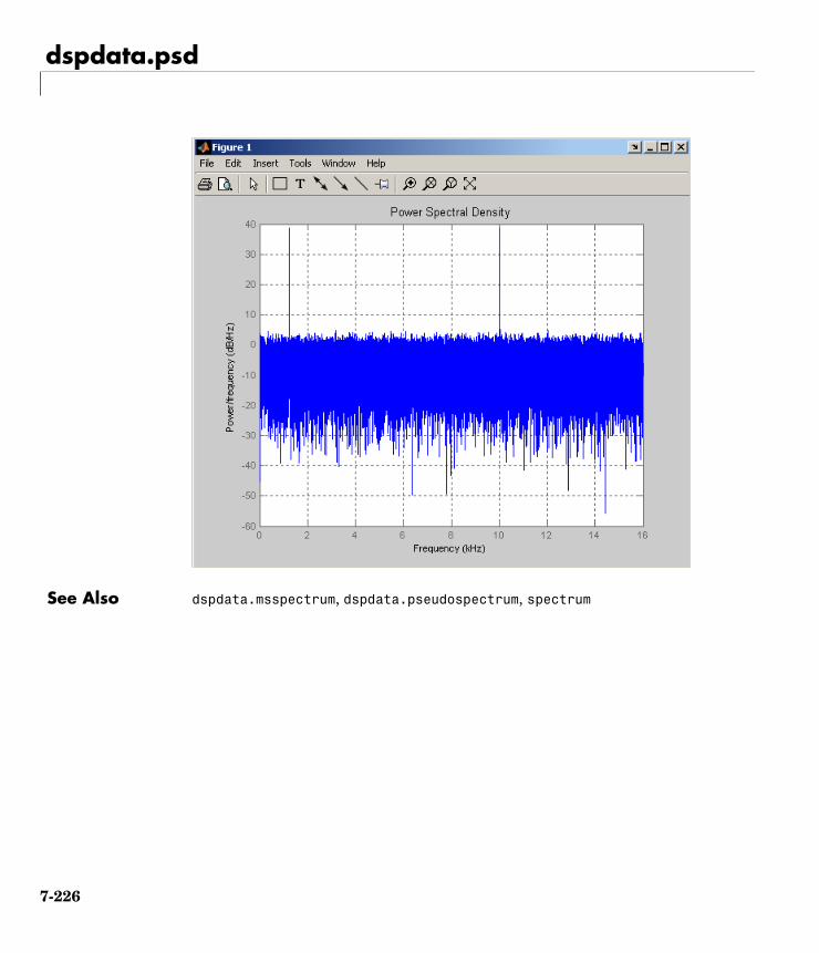
dspdata.psd
See Also dspdata.msspectrum, dspdata.pseudospectrum, spectrum
7-226
dspdata.pseudospectrum
7dspdata.pseudospectrumPurpose Create a pseudospectrum dspdata object
Syntax Hps = dspdata.pseudospectrum(Data)Hps = dspdata.pseudospectrum(Data,Frequencies)Hps = dspdata.pseudospectrum(...,'Fs',Fs)Hps = dspdata.pseudospectrum(...,'SpectrumRange',SpectrumRange)Hps = dspdata.pseudospectrum(...,'CenterDC',flag)
Description A pseudospectrum is an indicator of the presence of sinusoidal components in a signal.
Hps = dspdata.pseudospectrum(Data) uses the pseudospsectrum data contained in Data, which can be in the form of a vector or a matrix, where each column is a separate set of data. Default values for other properties of the object are:
7-227
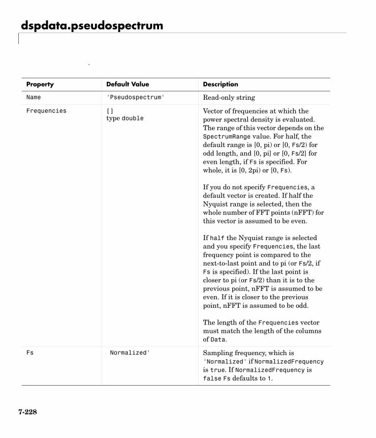
dspdata.pseudospectrum
.
Property Default Value Description
Name 'Pseudospectrum' Read-only string
Frequencies []type double
Vector of frequencies at which the power spectral density is evaluated. The range of this vector depends on the SpectrumRange value. For half, the default range is [0, pi) or [0, Fs/2) for odd length, and [0, pi] or [0, Fs/2] for even length, if Fs is specified. For whole, it is [0, 2pi) or [0, Fs).
If you do not specify Frequencies, a default vector is created. If half the Nyquist range is selected, then the whole number of FFT points (nFFT) for this vector is assumed to be even.
If half the Nyquist range is selected and you specify Frequencies, the last frequency point is compared to the next-to-last point and to pi (or Fs/2, if Fs is specified). If the last point is closer to pi (or Fs/2) than it is to the previous point, nFFT is assumed to be even. If it is closer to the previous point, nFFT is assumed to be odd.
The length of the Frequencies vector must match the length of the columns of Data.
Fs Normalized' Sampling frequency, which is 'Normalized' if NormalizedFrequency is true. If NormalizedFrequency is false Fs defaults to 1.
7-228
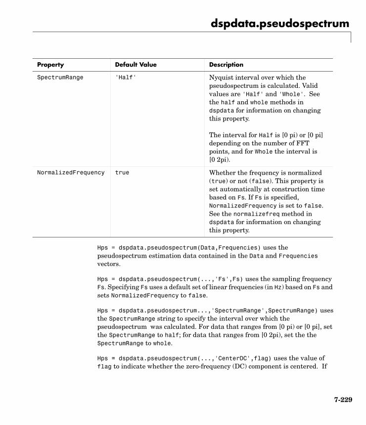
dspdata.pseudospectrum
Hps = dspdata.pseudospectrum(Data,Frequencies) uses the pseudospectrum estimation data contained in the Data and Frequencies vectors.
Hps = dspdata.pseudospectrum(...,'Fs',Fs) uses the sampling frequency Fs. Specifying Fs uses a default set of linear frequencies (in Hz) based on Fs and sets NormalizedFrequency to false.
Hps = dspdata.pseudospectrum...,'SpectrumRange',SpectrumRange) uses the SpectrumRange string to specify the interval over which the pseudospectrum was calculated. For data that ranges from [0 pi) or [0 pi], set the SpectrumRange to half; for data that ranges from [0 2pi), set the the SpectrumRange to whole.
Hps = dspdata.pseudospectrum(...,'CenterDC',flag) uses the value of flag to indicate whether the zero-frequency (DC) component is centered. If
SpectrumRange 'Half' Nyquist interval over which the pseudospectrum is calculated. Valid values are 'Half' and 'Whole'. See the half and whole methods in dspdata for information on changing this property.
The interval for Half is [0 pi) or [0 pi] depending on the number of FFT points, and for Whole the interval is [0 2pi).
NormalizedFrequency true Whether the frequency is normalized (true) or not (false). This property is set automatically at construction time based on Fs. If Fs is specified, NormalizedFrequency is set to false. See the normalizefreq method in dspdata for information on changing this property.
Property Default Value Description
7-229
dspdata.pseudospectrum
flag is true, it indicates that the DC component is in the center of the whole Nyquist range spectrum. Set the flag to false if the DC component is on the left edge of the spectrum.
MethodsMethods provide ways of performing functions directly on your dspdata object. You can apply a method directly on the variable you assigned to your dspdata.pseudospectrum object. You can use the following methods with a dspdata.pseudospectrum object.
• centerdc
• halfrange• normalizefreq• plot• wholerange
For example, to normalize the frequency and set the NormalizedFrequency parameter to true, use
Hps = normalizefreq(Hps)
For detailed information on using the methods and plotting the pseudospectrum, see the dspdata reference page.
Examples Storing and Plotting Pseudospectrum DataUse eigenanalysis to estimate the pseudospectrum of a noisy sinusoidal signal with two frequency components. Then store the results in a pseudospectrum data object and plot it.
Fs = 32e3;t = 0:1/Fs:2.96; x = cos(2*pi*t*1.24e3) + cos(2*pi*t*10e3) + randn(size(t)); P = pmusic(x,4);hps = dspdata.pseudospectrum(P,'Fs',Fs); % Create data object.plot(hps); % Plot the pseudospectrum.
7-230
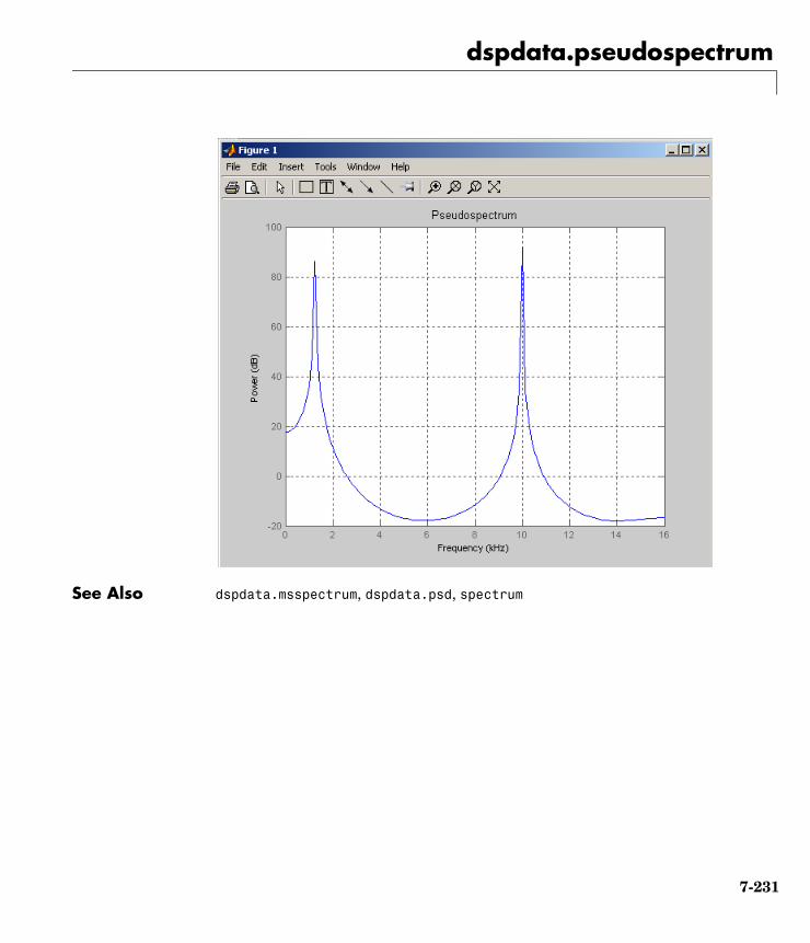
dspdata.pseudospectrum
See Also dspdata.msspectrum, dspdata.psd, spectrum
7-231
dspopts
7dspoptsPurpose DSP options objects
Syntax Hopts = dspopts.optsobj
Description Hopts = dspopts.optsobj returns a DSP options object Hopts of type optsobj. This DSP options object contains optional parameter information for the specified type of optsobj.
You create options objects via methods on other objects. For example,
Hopts = psdopts(Hs,X)
returns a spectrum object Hs options object. You can change the values of the Hopts object and then use this modified options object as an input to the psd method of a spectrum object Hs:
Hpsd = psd(Hs,X,psdopts)
Note You must use an optsobj with dspopts.
Options ObjectsAn options object (optsobj) for dspopts contain optional parameter values for the particular optsobj. Available optsobjs for dspopts are as follows:
• spectrum Spectrum options for any spectrum estimation method object. The spectrum object method to create this options object is psdopts and msspectrumopts. See spectrum for more information.
Properties and valid values of a dspopts.spectrum object are as follows:
- 'NFFT'—integer number of FFT points
- 'NormalizedFrequency'—whether frequency is normalized (true) or not (false)
- 'Fs'—sampling frequency, used only when 'NormalizedFrequency' is false. If 'NormalizedFrequency' is true, the value of Fs is 'Normalized'.
- 'SpectrumType' 'Onesided' for half the Nyquist interval or 'Twosided' for the whole Nyquist interval.
7-232
dspopts
• pseudospectrum Pseudospectrum options for spectrum.music and spectrum.eigenvector objects. The spectrum object method to create this options object is pseudospectrumopts. See spectrum for more information.
Properties and valid values of a dspopts.pseudospectrum object are as follows:
- 'NFFT'—integer number of FFT points
- 'NormalizedFreqeuncy'—whether frequency is normalized (true) or not (false)
- 'Fs'—sampling frequency, used only when 'NormalizedFrequency' is false. If 'NormalizedFrequency' is true, the value of Fs is 'Normalized'.
- 'SpectrumRange' 'Half' for half the Nyquist interval or 'Whole' for the whole Nyquist interval.
Modifying a DSPOPTS ObjectTo set specific properties, use
set(Hopts,'property1',value, 'property2',value,...)
or use the dot method
Hopts.property = value
where 'property1', 'property2', and property are the specific property names.
To view the options for a property use set without specifying a value
set(Hopts,'property')
Note that you must use single quotation marks around the property name if you are not using the dot method.
Another way to change an object’s properties is by using the inspect command, which opens the Property Inspector window where you can edit any property, except dynamic properties.
inspect(Hopts)
See Also spectrum, spectrum.burg, spectrum.cov, spectrum.eigenvector, spectrum.mcov, spectrum.mtm, spectrum.music, spectrum.periodogram, spectrum.welch, spectrum.yulear
7-233
ellip
7ellipPurpose Elliptic (Cauer) filter design
Syntax [b,a] = ellip(n,Rp,Rs,Wn)[b,a] = ellip(n,Rp,Rs,Wn,'ftype')[b,a] = ellip(n,Rp,Rs,Wn,'s')[b,a] = ellip(n,Rp,Rs,Wn,'ftype','s')[z,p,k] = ellip(...)[A,B,C,D] = ellip(...)
Description ellip designs lowpass, bandpass, highpass, and bandstop digital and analog elliptic filters. Elliptic filters offer steeper rolloff characteristics than Butterworth or Chebyshev filters, but are equiripple in both the pass- and stopbands. In general, elliptic filters meet given performance specifications with the lowest order of any filter type.
Digital Domain
[b,a] = ellip(n,Rp,Rs,Wn) designs an order n lowpass digital elliptic filter with normalized cutoff frequency Wn, Rp dB of ripple in the passband, and a stopband Rs dB down from the peak value in the passband. It returns the filter coefficients in the length n+1 row vectors b and a, with coefficients in descending powers of z.
The normalized cutoff frequency is the edge of the passband, at which the magnitude response of the filter is -Rp dB. For ellip, the normalized cutoff frequency Wn is a number between 0 and 1, where 1 corresponds to half the sampling frequency (Nyquist frequency). Smaller values of passband ripple Rp and larger values of stopband attenuation Rs both lead to wider transition widths (shallower rolloff characteristics).
If Wn is a two-element vector, Wn = [w1 w2], ellip returns an order 2*n bandpass filter with passband w1 < ω < w2.
[b,a] = ellip(n,Rp,Rs,Wn,'ftype') designs a highpass, lowpass, or bandstop filter, where the string 'ftype' is one of the following.
• 'high' for a highpass digital filter with normalized cutoff frequency Wn
H z( )B z( )A z( )----------- b 1( ) b 2( )z 1– b n 1+( )z n–+ + +
1 a 2( )z 1– a n 1+( )z n–+ + +------------------------------------------------------------------------------------= =
7-234

ellip
• 'low' for a lowpass digital filter with normalized cutoff frequency Wn
• 'stop' for an order 2*n bandstop digital filter if Wn is a two-element vector, Wn = [w1 w2]. The stopband is w1 < ω < w2.
With different numbers of output arguments, ellip directly obtains other realizations of the filter. To obtain zero-pole-gain form, use three output arguments as shown below.
[z,p,k] = ellip(n,Rp,Rs,Wn) or
[z,p,k] = ellip(n,Rp,Rs,Wn,'ftype') returns the zeros and poles in length n column vectors z and p and the gain in the scalar k.
To obtain state-space form, use four output arguments as shown below:
[A,B,C,D] = ellip(n,Rp,Rs,Wn) or
[A,B,C,D] = ellip(n,Rp,Rs,Wn,'ftype') where A, B, C, and D are
and u is the input, x is the state vector, and y is the output.
Analog Domain
[b,a] = ellip(n,Rp,Rs,Wn,'s') designs an order n lowpass analog elliptic filter with angular cutoff frequency Wn and returns the filter coefficients in the length n+1 row vectors b and a, in descending powers of s, derived from thistransfer function:
The angular cutoff frequency is the edge of the passband, at which the magnitude response of the filter is -Rp dB. For ellip, the angular cutoff frequency Wn must be greater than 0 rad/s.
If Wn is a two-element vector with w1 < w2, then ellip(n,Rp,Rs,Wn,'s') returns an order 2*n bandpass analog filter with passband w1 < ω < w2.
x n 1+[ ] Ax n[ ] Bu n[ ]+=
y n[ ] Cx n[ ] Du n[ ]+=
H s( )B s( )A s( )----------- b 1( )sn b 2( )sn 1– b n 1+( )+ + +
sn a 2( )sn 1– a n 1+( )+ + +-------------------------------------------------------------------------------------= =
7-235
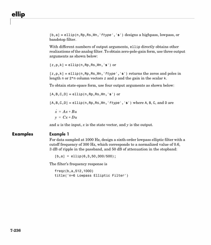
ellip
[b,a] = ellip(n,Rp,Rs,Wn,'ftype','s') designs a highpass, lowpass, or bandstop filter.
With different numbers of output arguments, ellip directly obtains other realizations of the analog filter. To obtain zero-pole-gain form, use three output arguments as shown below:
[z,p,k] = ellip(n,Rp,Rs,Wn,'s') or
[z,p,k] = ellip(n,Rp,Rs,Wn,'ftype','s') returns the zeros and poles in length n or 2*n column vectors z and p and the gain in the scalar k.
To obtain state-space form, use four output arguments as shown below:
[A,B,C,D] = ellip(n,Rp,Rs,Wn,'s') or
[A,B,C,D] = ellip(n,Rp,Rs,Wn,'ftype','s') where A, B, C, and D are
and u is the input, x is the state vector, and y is the output.
Examples Example 1For data sampled at 1000 Hz, design a sixth-order lowpass elliptic filter with a cutoff frequency of 300 Hz, which corresponds to a normalized value of 0.6, 3 dB of ripple in the passband, and 50 dB of attenuation in the stopband:
[b,a] = ellip(6,3,50,300/500);
The filter’s frequency response is
freqz(b,a,512,1000)title('n=6 Lowpass Elliptic Filter')
x· Ax Bu+=
y Cx Du+=
7-236
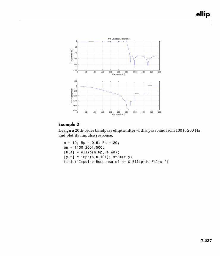
ellip
Example 2Design a 20th-order bandpass elliptic filter with a passband from 100 to 200 Hz and plot its impulse response:
n = 10; Rp = 0.5; Rs = 20;Wn = [100 200]/500;[b,a] = ellip(n,Rp,Rs,Wn);[y,t] = impz(b,a,101); stem(t,y)title('Impulse Response of n=10 Elliptic Filter')
0 50 100 150 200 250 300 350 400 450 500−500
−400
−300
−200
−100
0
100
Frequency (Hz)
Ph
ase
(d
eg
ree
s)0 50 100 150 200 250 300 350 400 450 500
−100
−80
−60
−40
−20
0
Frequency (Hz)
Ma
gn
itud
e (
dB
)
n=6 Lowpass Elliptic Filter
7-237
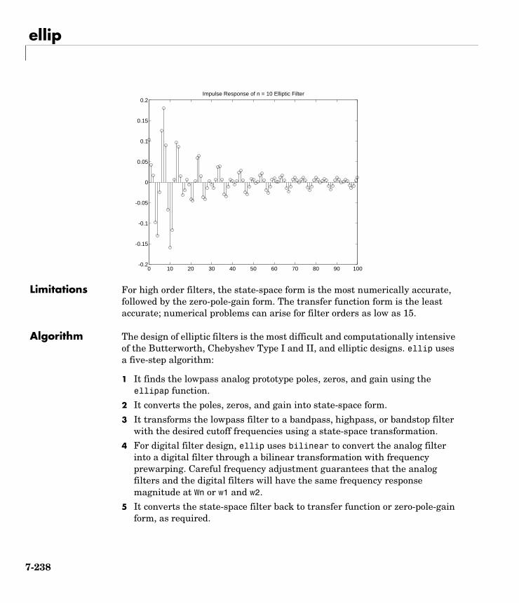
ellip
Limitations For high order filters, the state-space form is the most numerically accurate, followed by the zero-pole-gain form. The transfer function form is the least accurate; numerical problems can arise for filter orders as low as 15.
Algorithm The design of elliptic filters is the most difficult and computationally intensive of the Butterworth, Chebyshev Type I and II, and elliptic designs. ellip uses a five-step algorithm:
1 It finds the lowpass analog prototype poles, zeros, and gain using the ellipap function.
2 It converts the poles, zeros, and gain into state-space form.
3 It transforms the lowpass filter to a bandpass, highpass, or bandstop filter with the desired cutoff frequencies using a state-space transformation.
4 For digital filter design, ellip uses bilinear to convert the analog filter into a digital filter through a bilinear transformation with frequency prewarping. Careful frequency adjustment guarantees that the analog filters and the digital filters will have the same frequency response magnitude at Wn or w1 and w2.
5 It converts the state-space filter back to transfer function or zero-pole-gain form, as required.
0 10 20 30 40 50 60 70 80 90 100-0.2
-0.15
-0.1
-0.05
0
0.05
0.1
0.15
0.2Impulse Response of n = 10 Elliptic Filter
7-238

ellip
See Also besself, butter, cheby1, cheby2, ellipap, ellipord
7-239
ellipap
7ellipapPurpose Elliptic analog lowpass filter prototype
Syntax [z,p,k] = ellipap(n,Rp,Rs)
Description [z,p,k] = ellipap(n,Rp,Rs) returns the zeros, poles, and gain of an order n elliptic analog lowpass filter prototype, with Rp dB of ripple in the passband, and a stopband Rs dB down from the peak value in the passband. The zeros and poles are returned in length n column vectors z and p and the gain in scalar k. If n is odd, z is length n - 1. The transfer function is
Elliptic filters offer steeper rolloff characteristics than Butterworth and Chebyshev filters, but they are equiripple in both the passband and the stopband. Of the four classical filter types, elliptic filters usually meet a given set of filter performance specifications with the lowest filter order.
ellip sets the cutoff angular frequency of the elliptic filter to 1 for a normalized result. The cutoff angular frequency is the frequency at which the passband ends and the filter has a magnitude response of 10-Rp/20.
Algorithm ellipap uses the algorithm outlined in [1]. It employs the M-file ellipk to calculate the complete elliptic integral of the first kind and the M-file ellipj to calculate Jacobi elliptic functions.
See Also besselap, buttap, cheb1ap, cheb2ap, ellip
References [1] Parks, T.W., and C.S. Burrus. Digital Filter Design. New York: John Wiley & Sons, 1987. Chapter 7.
H s( )z s( )p s( )---------- k s z 1( )–( ) s z 2( )–( ) s z n( )–( )
s p 1( )–( ) s p 2( )–( ) s p n( )–( )--------------------------------------------------------------------------------= =
ω0
7-240
ellipord
7ellipordPurpose Calculate the minimum order for elliptic filters
Syntax [n,Wn] = ellipord(Wp,Ws,Rp,Rs)[n,Wn] = ellipord(Wp,Ws,Rp,Rs,'s')
Description ellipord calculates the minimum order of a digital or analog elliptic filter required to meet a set of filter design specifications.
Digital Domain
[n,Wn] = ellipord(Wp,Ws,Rp,Rs) returns the lowest order n of the elliptic filter that loses no more than Rp dB in the passband and has at least Rs dB of attenuation in the stopband. The scalar (or vector) of corresponding cutoff frequencies Wn, is also returned. Use the output arguments n and Wn in ellip.
Choose the input arguments to specify the stopband and passband according to the following table.
Description of Stopband and Passband Filter Parameters
Parameter Description
Wp Passband corner frequency Wp, the cutoff frequency, is a scalar or a two-element vector with values between 0 and 1, with 1 corresponding to the normalized Nyquist frequency, π radians per sample.
Ws Stopband corner frequency Ws, is a scalar or a two-element vector with values between 0 and 1, with 1 corresponding to the normalized Nyquist frequency.
Rp Passband ripple, in decibels. Twice this value specifies the maximum permissible passband width in decibels.
Rs Stopband attenuation, in decibels. This value is the number of decibels the stopband is attenuated with respect to the passband response.
7-241
ellipord
Use the following guide to specify filters of different types.
If your filter specifications call for a bandpass or bandstop filter with unequal ripple in each of the passbands or stopbands, design separate lowpass and highpass filters according to the specifications in this table, and cascade the two filters together.
Analog Domain
[n,Wn] = ellipord(Wp,Ws,Rp,Rs,'s') finds the minimum order n and cutoff frequencies Wn for an analog filter. You specify the frequencies Wp and Ws similar to those described in the Table , Description of Stopband and Passband Filter Parameters table above, only in this case you specify the frequency in radians per second, and the passband or the stopband can be infinite.
Use ellipord for lowpass, highpass, bandpass, and bandstop filters as described in the Table , Filter Type Stopband and Passband Specifications table above.
Filter Type Stopband and Passband Specifications
Filter Type Stopband and Passband Conditions Stopband Passband
Lowpass Wp < Ws, both scalars (Ws,1) (0,Wp)
Highpass Wp > Ws, both scalars (0,Ws) (Wp,1)
Bandpass The interval specified by Ws contains the one specified by Wp (Ws(1) < Wp(1) < Wp(2) < Ws(2)).
(0,Ws(1)) and (Ws(2),1)
(Wp(1),Wp(2))
Bandstop The interval specified by Wp contains the one specified by Ws (Wp(1) < Ws(1) < Ws(2) < Wp(2)).
(0,Wp(1)) and (Wp(2),1)
(Ws(1),Ws(2))
7-242
ellipord
Examples Example 1For 1000 Hz data, design a lowpass filter with less than 3 dB of ripple in the passband defined from 0 to 40 Hz and at least 60 dB of ripple in the stopband defined from 150 Hz to the Nyquist frequency (500 Hz):
Wp = 40/500; Ws = 150/500;Rp = 3; Rs = 60;[n,Wn] = ellipord(Wp,Ws,Rp,Rs)
n = 4
Wn = 0.0800
[b,a] = ellip(n,Rp,Rs,Wn);freqz(b,a,512,1000);title('n=4 Elliptic Lowpass Filter')
0 50 100 150 200 250 300 350 400 450 500−400
−300
−200
−100
0
100
Frequency (Hz)
Ph
ase
(d
eg
ree
s)
0 50 100 150 200 250 300 350 400 450 500−120
−100
−80
−60
−40
−20
0
Frequency (Hz)
Ma
gn
itud
e (
dB
)
n=4 Elliptic Lowpass Filter
7-243
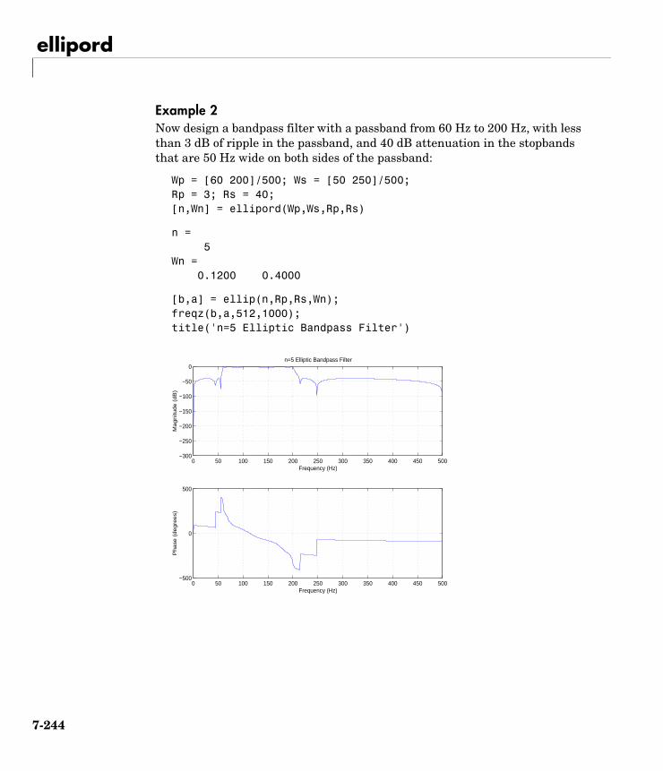
ellipord
Example 2Now design a bandpass filter with a passband from 60 Hz to 200 Hz, with less than 3 dB of ripple in the passband, and 40 dB attenuation in the stopbands that are 50 Hz wide on both sides of the passband:
Wp = [60 200]/500; Ws = [50 250]/500;Rp = 3; Rs = 40;[n,Wn] = ellipord(Wp,Ws,Rp,Rs)
n = 5Wn = 0.1200 0.4000
[b,a] = ellip(n,Rp,Rs,Wn);freqz(b,a,512,1000);title('n=5 Elliptic Bandpass Filter')
0 50 100 150 200 250 300 350 400 450 500−500
0
500
Frequency (Hz)
Ph
ase
(d
eg
ree
s)
0 50 100 150 200 250 300 350 400 450 500−300
−250
−200
−150
−100
−50
0
Frequency (Hz)
Ma
gn
itud
e (
dB
)
n=5 Elliptic Bandpass Filter
7-244
ellipord
Algorithm ellipord uses the elliptic lowpass filter order prediction formula described in [1]. The function performs its calculations in the analog domain for both the analog and digital cases. For the digital case, it converts the frequency parameters to the s-domain before estimating the order and natural frequencies, and then converts them back to the z-domain.
ellipord initially develops a lowpass filter prototype by transforming the passband frequencies of the desired filter to 1 rad/s (for low- and highpass filters) and to -1 and 1 rad/s (for bandpass and bandstop filters). It then computes the minimum order required for a lowpass filter to meet the stopband specification.
See Also buttord, cheb1ord, cheb2ord, ellip
References [1] Rabiner, L.R., and B. Gold. Theory and Application of Digital Signal Processing. Englewood Cliffs, NJ: Prentice-Hall, 1975. Pg. 241.
7-245
eqtflength
7eqtflengthPurpose Make the lengths of a transfer function’s numerator and denominator equal
Syntax [b,a] = eqtflength(num,den)[b,a,n,m] = eqtflength(num,den)
Description [b,a] = eqtflength(num,den) modifies the vector num and/or the vector den, so that the resulting output vectors b and a have the same length. The input vectors num and den may have different lengths. The vector num represents the numerator polynomial of a given discrete-time transfer function, and the vector den represents its denominator. The resulting numerator b and denominator a represent the same discrete-time transfer function, but these vectors have the same length.
[b,a,n,m] = eqtflength(num,den) modifies the vectors as above and also returns the numerator order n and the denominator m, not including any trailing zeros.
Use eqtflength to obtain a numerator and denominator of equal length before applying transfer function conversion functions such as tf2ss and tf2zp to discrete-time models.
Examples num = [1 0.5];den = [1 0.75 0.6 0];[b,a,n,m] = eqtflength(num,den)
b = 1.0000 0.5000 0
a = 1.0000 0.7500 0.6000
n = 1m = 2
Algorithm eqtflength(num,den) appends zeros to either num or den as necessary. If both num and den have trailing zeros in common, these are removed.
See Also tf2ss, tf2zp
7-246
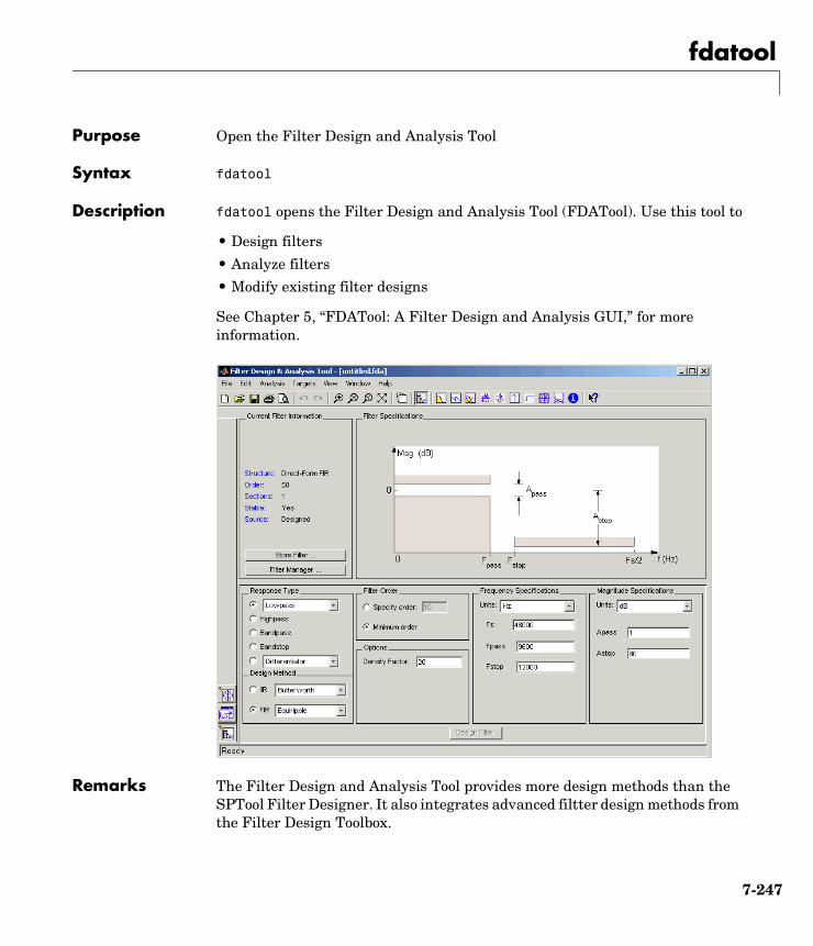
fdatool
7fdatoolPurpose Open the Filter Design and Analysis Tool
Syntax fdatool
Description fdatool opens the Filter Design and Analysis Tool (FDATool). Use this tool to
• Design filters
• Analyze filters
• Modify existing filter designs
See Chapter 5, “FDATool: A Filter Design and Analysis GUI,” for more information.
Remarks The Filter Design and Analysis Tool provides more design methods than the SPTool Filter Designer. It also integrates advanced filtter design methods from the Filter Design Toolbox.
7-247

fdatool
Note The Filter Design and Analysis Tool requires a screen resolution greater than 640 x 480.
See Also fvtool, sptool, wvtool
7-248

fft
7fftPurpose Compute the one-dimensional fast Fourier transform
fft is a MATLAB function.
7-249

fft2
7fft2Purpose Compute the two-dimensional fast Fourier transform
fft2 is a MATLAB function.
7-250
fftfilt
7fftfiltPurpose FFT-based FIR filtering using the overlap-add method
Syntax y = fftfilt(b,x)y = fftfilt(b,x,n)
Description fftfilt filters data using the efficient FFT-based method of overlap-add, a frequency domain filtering technique that works only for FIR filters.
y = fftfilt(b,x) filters the data in vector x with the filter described by coefficient vector b. It returns the data vector y. The operation performed by fftfilt is described in the time domain by the difference equation:
An equivalent representation is the z-transform or frequency domain description:
By default, fftfilt chooses an FFT length and data block length that guarantee efficient execution time.
y = fftfilt(b,x,n) uses an FFT length of nfft = 2^nextpow2(n) and a data block length of nfft - length(b) + 1.
fftfilt works for both real and complex inputs.
Examples Show that the results from fftfilt and filter are identical:
b = [1 2 3 4];x = [1 zeros(1,99)]';norm(fftfilt(b,x) - filter(b,1,x))
ans =9.5914e-15
y n( ) b 1( )x n( ) b 2( )x n 1–( ) b nb 1+( )x n nb–( )+ + +=
Y z( ) b 1( ) b 2( )z 1– b nb 1+( )z nb–+ + +( )X z( )=
7-251
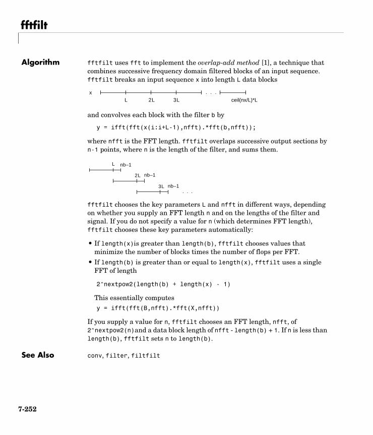
fftfilt
Algorithm fftfilt uses fft to implement the overlap-add method [1], a technique that combines successive frequency domain filtered blocks of an input sequence. fftfilt breaks an input sequence x into length L data blocks
and convolves each block with the filter b by
y = ifft(fft(x(i:i+L-1),nfft).*fft(b,nfft));
where nfft is the FFT length. fftfilt overlaps successive output sections by n-1 points, where n is the length of the filter, and sums them.
fftfilt chooses the key parameters L and nfft in different ways, depending on whether you supply an FFT length n and on the lengths of the filter and signal. If you do not specify a value for n (which determines FFT length), fftfilt chooses these key parameters automatically:
• If length(x)is greater than length(b), fftfilt chooses values that minimize the number of blocks times the number of flops per FFT.
• If length(b) is greater than or equal to length(x), fftfilt uses a single FFT of length
2^nextpow2(length(b) + length(x) - 1)
This essentially computesy = ifft(fft(B,nfft).*fft(X,nfft))
If you supply a value for n, fftfilt chooses an FFT length, nfft, of 2^nextpow2(n)and a data block length of nfft - length(b) + 1. If n is less than length(b), fftfilt sets n to length(b).
See Also conv, filter, filtfilt
xL 2L 3L ceil(nx/L)*L
. . .
nb–1L
nb–12L
nb–13L. . .
7-252

fftfilt
References [1] Oppenheim, A.V., and R.W. Schafer, Discrete-Time Signal Processing, Prentice-Hall, 1989.
7-253

fftshift
7fftshiftPurpose Rearrange the outputs of the FFT functions
fftshift is a MATLAB function.
7-254
filter
7filterPurpose Filter data with a recursive (IIR) or nonrecursive (FIR) filter
filter is a MATLAB function.
Signal-specific Information
Filter Method of DFILTFilter is also an overloaded method of the discrete-time filter object (dfilt). You can pass an object handle, data, and initial conditions into the filter method. Note, however, that the recommended method of passing initial conditions into a dfilt is by using the states method. For more information, see the dfilt reference page.
Filter NormalizationUsing filter on b and a coefficients normalizes the filter by forcing the a0 coefficient to be equal to 1.
Using the filter method on a dfilt object does not normalize the a0 coefficient.
7-255

filter2
7filter2Purpose Two-dimensional digital filtering
filter2 is a MATLAB function.
7-256
filternorm
7filternormPurpose Compute the 2-norm or infinity-norm of a digital filter
Syntax filternorm(b,a)filternorm(b,a,pnorm)
filternorm(b,a,2,tol)
Description A typical use for filter norms is in digital filter scaling to reduce quantization effects. Scaling often improves the signal-to-noise ratio of the filter without resulting in data overflow. You, also, can use the 2-norm to compute the energy of the impulse response of a filter.
filternorm(b,a) computes the 2-norm of the digital filter defined by the numerator coefficients in b and denominator coefficients in a.
filternorm(b,a,pnorm) computes the 2- or infinity-norm (inf-norm) of the digital filter, where pnorm is either 2 or inf.
filternorm(b,a,2,tol) computes the 2-norm of an IIR filter with the specified tolerance, tol. The tolerance can be specified only for IIR 2-norm computations. pnorm in this case must be 2. If tol is not specified, it defaults to 1e-8.
Examples Compute the 2-norm with a tolerance of 1e-10 of an IIR filter:
[b,a]=butter(5,.5);L2=filternorm(b,a,2,1e-10)
L2 =
0.7071
Compute the inf-norm of an FIR filter:
b=firpm(30,[.1 .9],[1 1],'Hilbert');Linf=filternorm(b,1,inf)
Linf =
1.0028
7-257
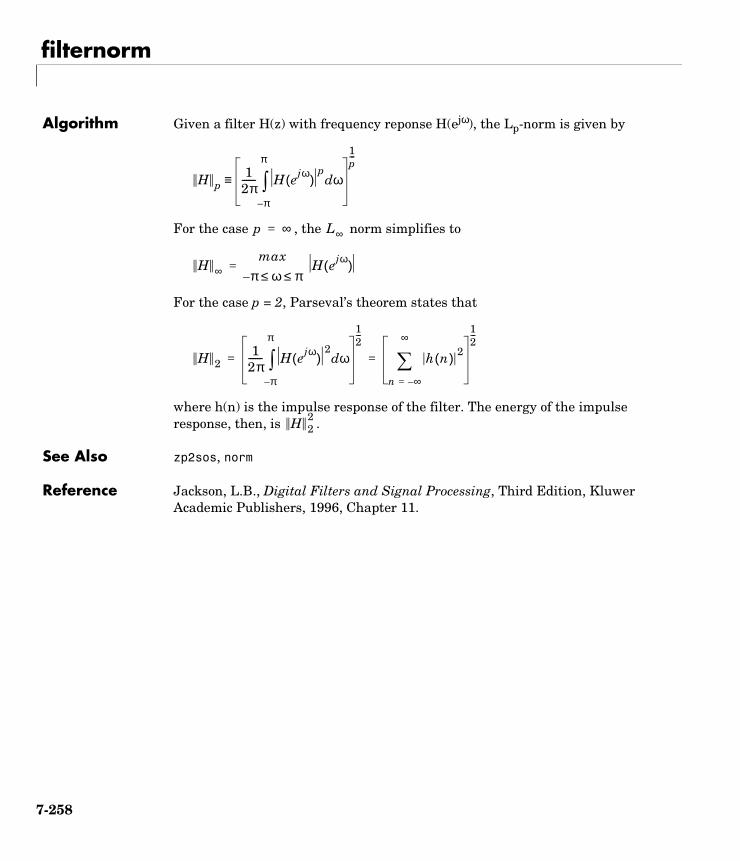
filternorm
Algorithm Given a filter H(z) with frequency reponse H(ejω), the Lp-norm is given by
For the case , the norm simplifies to
For the case p = 2, Parseval’s theorem states that
where h(n) is the impulse response of the filter. The energy of the impulse response, then, is .
See Also zp2sos, norm
Reference Jackson, L.B., Digital Filters and Signal Processing, Third Edition, Kluwer Academic Publishers, 1996, Chapter 11.
H p1
2π------ H ejω( )
pωd
π–
π
∫
1p---
≡
p ∞= L∞
H ∞max
π ω π≤ ≤–H ejω( )=
H 21
2π------ H ejω( )
2ωd
π–
π
∫
12---
h n( ) 2
n ∞–=
∞
∑
12---
= =
H 22
7-258
filtfilt
7filtfiltPurpose Zero-phase digital filtering
Syntax y = filtfilt(b,a,x)
Description y = filtfilt(b,a,x) performs zero-phase digital filtering by processing the input data in both the forward and reverse directions (see problem 5.39 in [1]). After filtering in the forward direction, it reverses the filtered sequence and runs it back through the filter. The resulting sequence has precisely zero-phase distortion and double the filter order. filtfilt minimizes start-up and ending transients by matching initial conditions, and works for both real and complex inputs.
Note that filtfilt should not be used with differentiator and Hilbert FIR filters, since the operation of these filters depends heavily on their phase response.
Algorithm filtfilt is an M-file that uses the filter function. In addition to the forward-reverse filtering, it attempts to minimize startup transients by adjusting initial conditions to match the DC component of the signal and by prepending several filter lengths of a flipped, reflected copy of the input signal.
See Also fftfilt, filter, filter2
References [1] Oppenheim, A.V., and R.W. Schafer, Discrete-Time Signal Processing, Prentice-Hall, 1989, pp. 311-312.
[2] Mitra, S.K., Digital Signal Processing, 2nd ed., McGraw-Hill, 2001, Sections 4.4.2 and 8.2.5.
[3] Gustafsson, F., “Determining the initial states in forward-backward filtering,” IEEE Transactions on Signal Processing, April 1996, Volume 44, Issue 4, pp. 988--992,
7-259
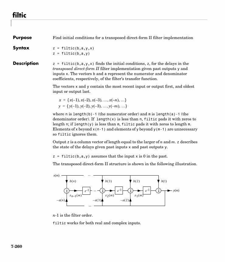
filtic
7filticPurpose Find initial conditions for a transposed direct-form II filter implementation
Syntax z = filtic(b,a,y,x)z = filtic(b,a,y)
Description z = filtic(b,a,y,x) finds the initial conditions, z, for the delays in the transposed direct-form II filter implementation given past outputs y and inputs x. The vectors b and a represent the numerator and denominator coefficients, respectively, of the filter’s transfer function.
The vectors x and y contain the most recent input or output first, and oldest input or output last.
where n is length(b)-1 (the numerator order) and m is length(a)-1 (the denominator order). If length(x) is less than n, filtic pads it with zeros to length n; if length(y) is less than m, filtic pads it with zeros to length m. Elements of x beyond x(n-1) and elements of y beyond y(m-1) are unnecessary so filtic ignores them.
Output z is a column vector of length equal to the larger of n and m. z describes the state of the delays given past inputs x and past outputs y.
z = filtic(b,a,y) assumes that the input x is 0 in the past.
The transposed direct-form II structure is shown in the following illustration.
n-1 is the filter order.
filtic works for both real and complex inputs.
x x 1–( ) x 2–( ) x 3–( ) … x n–( ) …, , , , , =
y y 1–( ) y 2–( ) y 3–( ) … y m–( ) …, , , , , =
Σ Σ Σz -1 z -1
x(m)
y(m)
b(3) b(2) b(1)
– a(3) – a(2)
z1(m)z2(m)Σ z -1
b(n)
–a(n)
zn -1(m)
...
...
...
7-260
filtic
Algorithm filtic performs a reverse difference equation to obtain the delay states z.
Diagnostics If any of the input arguments y, x, b, or a is not a vector (that is, if any argument is a scalar or array), filtic gives the following error message:
Requires vector inputs.
See Also filter, filtfilt
References Oppenheim, A.V., and R.W. Schafer, Discrete-Time Signal Processing, Prentice-Hall, 1989, pp. 296, 301-302.
7-261
filtstates
7filtstatesPurpose Filter states objects
Syntax Hs = filtstates.dfiir(numstates,denstates)
Description Hs = filtstates.dfiir(numstates,denstates) returns an IIR direct-form filter states object Hs with two properties—Numerator and Denominator, which contain the filter states. These two properties are column vectors with each column representing a separate channel of filter states. The number of states is always one less than the the number of filter numerator or denominator coefficients.
You can extract a filtstates object from the states property of an IIR direct-form I object with
Hd = dfilt.df1Hs = Hd.states
Note filtstates are used only with IIR Direct-form I filters (dfilt.df1, dfilt.df1t, dfilt.df1sos, and dfilt.df1tsos).
MethodsYou can use the following methods on a filtstates object.
Examples This example demonstrates the interaction of filtstates with a dfilt.df1 object.
Method Description
double Converts a filtstates object to a double-precision vector containing the values of the numerator and denominator states. The numerator states are listed first in this vector, followed by the denominator states.
single Converts a filtstates object to a single-precision vector containing the values of the numerator and denominator states. (This method is used with the Fitler Design Toolbox.)
7-262
filtstates
[b,a] = butter(4,0.5); % Design a butterworth filterHd = dfilt.df1(b,a); % Create a dfilt objectHs = Hd.states % Extract a filter states object from
% the dfilt states propertyHs.Numerator = [1,1,1,1]' % Modify the numerator statesHd.states = Hs % Set the modified states back to the
% original object
Dbl = double(Hs) % Create a double vector from states
See Also dfilt, dfilt.df1, dfilt.df1t, dfilt.df1sos, dfilt.df1tsos
7-263
fir1
7fir1Purpose Design a window-based finite impulse response filter
Syntax b = fir1(n,Wn)b = fir1(n,Wn,'ftype')b = fir1(n,Wn,window)b = fir1(n,Wn,'ftype',window)b = fir1(...,'normalization')
Description fir1 implements the classical method of windowed linear-phase FIR digital filter design [1]. It designs filters in standard lowpass, highpass, bandpass, and bandstop configurations. By default the filter is normalized so that the magnitude response of the filter at the center frequency of the passband is 0 dB.
Note Use fir2 for windowed filters with arbitrary frequency response.
b = fir1(n,Wn) returns row vector b containing the n+1 coefficients of an order n lowpass FIR filter. This is a Hamming-window based, linear-phase filter with normalized cutoff frequency Wn. The output filter coefficients, b, are ordered in descending powers of z.
Wn is a number between 0 and 1, where 1 corresponds to the Nyquist frequency.
If Wn is a two-element vector, Wn = [w1 w2], fir1 returns a bandpass filter with passband w1 < ω < w2.
If Wn is a multi-element vector, Wn = [w1 w2 w3 w4 w5 ... wn], fir1 returns an order n multiband filter with bands 0 < ω < w1, w1 < ω < w2, ..., wn < ω < 1.
By default, the filter is scaled so that the center of the first passband has a magnitude of exactly 1 after windowing.
b = fir1(n,Wn,'ftype') specifies a filter type, where 'ftype' is:
• 'high' for a highpass filter with cutoff frequency Wn.
B z( ) b 1( ) b 2( )z 1– b n 1+( )z n–+ + +=
7-264
fir1
• 'stop' for a bandstop filter, if Wn = [w1 w2]. The stopband frequency range is specified by this interval.
• 'DC-1' to make the first band of a multiband filter a passband.
• 'DC-0' to make the first band of a multiband filter a stopband.
fir1 always uses an even filter order for the highpass and bandstop configurations. This is because for odd orders, the frequency response at the Nyquist frequency is 0, which is inappropriate for highpass and bandstop filters. If you specify an odd-valued n, fir1 increments it by 1.
b = fir1(n,Wn,window) uses the window specified in column vector window for the design. The vector window must be n+1 elements long. If no window is specified, fir1 uses a Hamming window (see hamming) of length n+1.
b = fir1(n,Wn,'ftype',window) accepts both 'ftype' and window parameters.
b = fir1(...,'normalization') specifies whether or not the filter magnitude is normalized. The string 'normalization' can be the following:
• 'scale' (default): Normalize the filter so that the magnitude response of the filter at the center frequency of the passband is 0 dB.
• 'noscale': Do not normalize the filter.
The group delay of the FIR filter designed by fir1 is n/2.
Algorithm fir1 uses the window method of FIR filter design [1]. If w(n) denotes a window, where 1 ≤ n ≤ N, and the impulse response of the ideal filter is h(n), where h(n) is the inverse Fourier transform of the ideal frequency response, then the windowed digital filter coefficients are given by
b n( ) w n( )h n( ) 1 n N≤ ≤,=
7-265
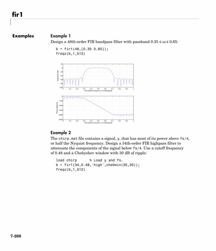
fir1
Examples Example 1Design a 48th-order FIR bandpass filter with passband 0.35 ≤ ω ≤ 0.65:
b = fir1(48,[0.35 0.65]);freqz(b,1,512)
Example 2The chirp.mat file contains a signal, y, that has most of its power above fs/4, or half the Nyquist frequency. Design a 34th-order FIR highpass filter to attenuate the components of the signal below fs/4. Use a cutoff frequency of 0.48 and a Chebyshev window with 30 dB of ripple:
load chirp % Load y and fs.b = fir1(34,0.48,'high',chebwin(35,30));freqz(b,1,512)
0 0.1 0.2 0.3 0.4 0.5 0.6 0.7 0.8 0.9 1−2500
−2000
−1500
−1000
−500
0
Normalized Frequency (×π rad/sample)
Pha
se (
degr
ees)
0 0.1 0.2 0.3 0.4 0.5 0.6 0.7 0.8 0.9 1−100
−80
−60
−40
−20
0
20
Normalized Frequency (×π rad/sample)
Mag
nitu
de (
dB)
7-266
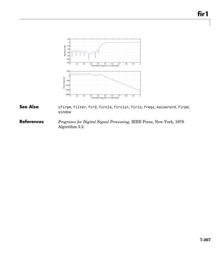
fir1
See Also cfirpm, filter, fir2, fircls, fircls1, firls, freqz, kaiserord, firpm, window
References Programs for Digital Signal Processing, IEEE Press, New York, 1979. Algorithm 5.2.
0 0.1 0.2 0.3 0.4 0.5 0.6 0.7 0.8 0.9 1−2000
−1500
−1000
−500
0
500
Normalized Frequency (×π rad/sample)
Pha
se (
degr
ees)
0 0.1 0.2 0.3 0.4 0.5 0.6 0.7 0.8 0.9 1−120
−100
−80
−60
−40
−20
0
20
Normalized Frequency (×π rad/sample)M
agni
tude
(dB
)
7-267
fir2
7fir2Purpose Design a frequency sampling-based finite impulse response filter
Syntax b = fir2(n,f,m)b = fir2(n,f,m,window)b = fir2(n,f,m,npt)b = fir2(n,f,m,npt,window)b = fir2(n,f,m,npt,lap)b = fir2(n,f,m,npt,lap,window)
Description fir2 designs frequency sampling-based digital FIR filters with arbitrarily shaped frequency response.
Note Use fir1 for windows-based standard lowpass, bandpass, highpass, and bandstop configurations.
b = fir2(n,f,m) returns row vector b containing the n+1 coefficients of an order n FIR filter. The frequency-magnitude characteristics of this filter match those given by vectors f and m:
• f is a vector of frequency points in the range from 0 to 1, where 1 corresponds to the Nyquist frequency. The first point of f must be 0 and the last point 1. The frequency points must be in increasing order.
• m is a vector containing the desired magnitude response at the points specified in f.
• f and m must be the same length.
• Duplicate frequency points are allowed, corresponding to steps in the frequency response.
Use plot(f,m) to view the filter shape.
The output filter coefficients, b, are ordered in descending powers of z.
fir2 always uses an even filter order for configurations with a passband at the Nyquist frequency. This is because for odd orders, the frequency response at
b z( ) b 1( ) b 2( )z 1– b n 1+( )z n–+ + +=
7-268
fir2
the Nyquist frequency is necessarily 0. If you specify an odd-valued n, fir2 increments it by 1.
b = fir2(n,f,m,window) uses the window specified in the column vector window. The vector window must be n+1 elements long. If no window is specified, fir2 uses a Hamming window (see hamming) of length n+1.
b = fir2(n,f,m,npt) or
b = fir2(n,f,m,npt,window) specifies the number of points, npt, for the grid onto which fir2 interpolates the frequency response, without or with a window specification.
b = fir2(n,f,m,npt,lap) and
b = fir2(n,f,m,npt,lap,window) specify the size of the region, lap, that fir2 inserts around duplicate frequency points, with or without a window specification.
See the “Algorithm” section for more on npt and lap.
Examples Design a 30th-order lowpass filter and overplot the desired frequency response with the actual frequency response:
f = [0 0.6 0.6 1]; m = [1 1 0 0];b = fir2(30,f,m);[h,w] = freqz(b,1,128);plot(f,m,w/pi,abs(h))legend('Ideal','fir2 Designed')title('Comparison of Frequency Response Magnitudes')
7-269
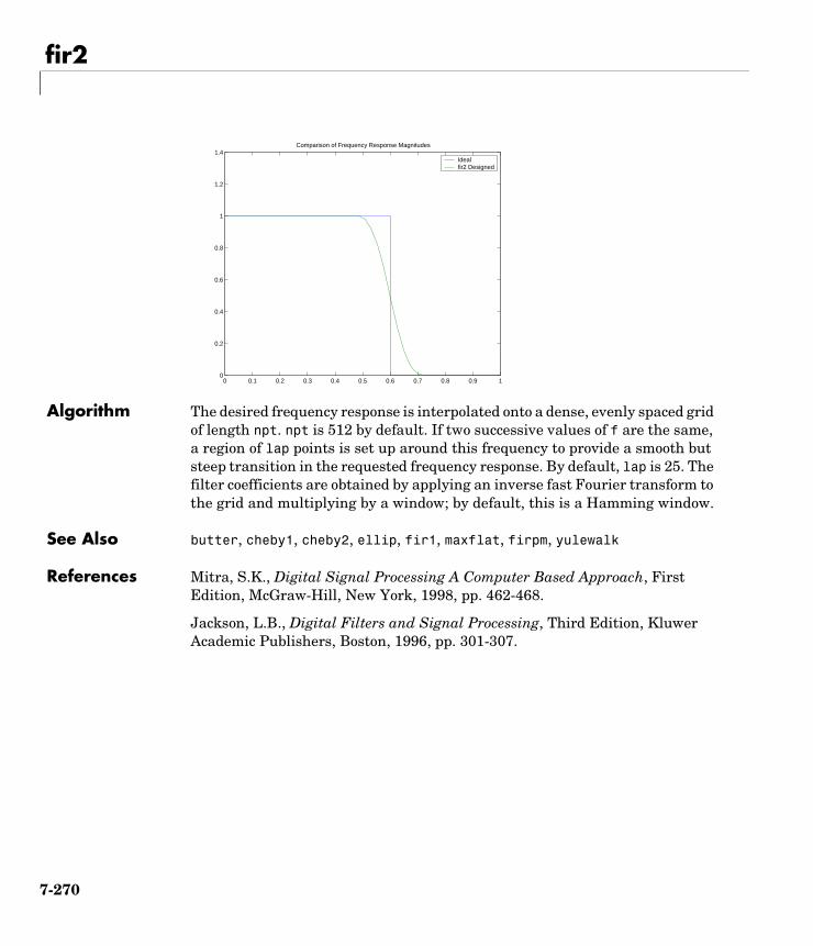
fir2
Algorithm The desired frequency response is interpolated onto a dense, evenly spaced grid of length npt. npt is 512 by default. If two successive values of f are the same, a region of lap points is set up around this frequency to provide a smooth but steep transition in the requested frequency response. By default, lap is 25. The filter coefficients are obtained by applying an inverse fast Fourier transform to the grid and multiplying by a window; by default, this is a Hamming window.
See Also butter, cheby1, cheby2, ellip, fir1, maxflat, firpm, yulewalk
References Mitra, S.K., Digital Signal Processing A Computer Based Approach, First Edition, McGraw-Hill, New York, 1998, pp. 462-468.
Jackson, L.B., Digital Filters and Signal Processing, Third Edition, Kluwer Academic Publishers, Boston, 1996, pp. 301-307.
0 0.1 0.2 0.3 0.4 0.5 0.6 0.7 0.8 0.9 10
0.2
0.4
0.6
0.8
1
1.2
1.4Comparison of Frequency Response Magnitudes
Ideal fir2 Designed
7-270
fircls
7firclsPurpose Constrained least square FIR filter design for multiband filters
Syntax b = fircls(n,f,amp,up,lo)fircls(n,f,amp,up,lo,'design_flag')
Description b = fircls(n,f,amp,up,lo) generates a length n+1 linear phase FIR filter b. The frequency-magnitude characteristics of this filter match those given by vectors f and amp:
• f is a vector of transition frequencies in the range from 0 to 1, where 1 corresponds to the Nyquist frequency. The first point of f must be 0 and the last point 1. The frequency points must be in increasing order.
• amp is a vector describing the piecewise constant desired amplitude of the frequency response. The length of amp is equal to the number of bands in the response and should be equal to length(f)-1.
• up and lo are vectors with the same length as amp. They define the upper and lower bounds for the frequency response in each band.
fircls always uses an even filter order for configurations with a passband at the Nyquist frequency. This is because for odd orders, the frequency response at the Nyquist frequency is necessarily 0. If you specify an odd-valued n, fircls increments it by 1.
fircls(n,f,amp,up,lo,'design_flag') enables you to monitor the filter design, where 'design_flag' can be
• 'trace', for a textual display of the design error at each iteration step.
• 'plots', for a collection of plots showing the filter’s full-band magnitude response and a zoomed view of the magnitude response in each sub-band. All plots are updated at each iteration step.
• 'both', for both the textual display and plots.
7-271
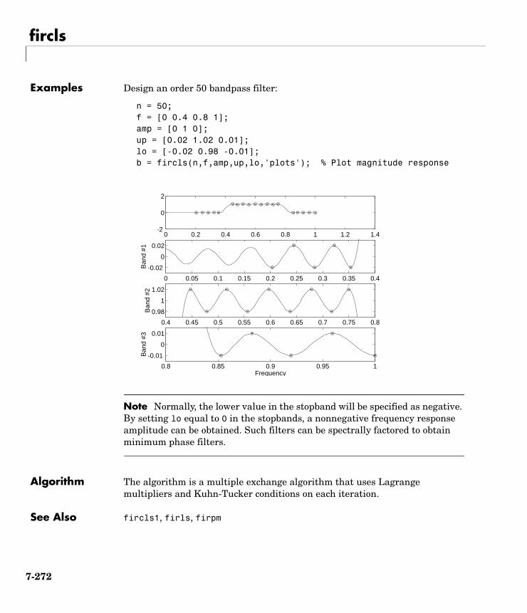
fircls
Examples Design an order 50 bandpass filter:
n = 50;f = [0 0.4 0.8 1];amp = [0 1 0];up = [0.02 1.02 0.01];lo = [-0.02 0.98 -0.01];b = fircls(n,f,amp,up,lo,'plots'); % Plot magnitude response
Note Normally, the lower value in the stopband will be specified as negative. By setting lo equal to 0 in the stopbands, a nonnegative frequency response amplitude can be obtained. Such filters can be spectrally factored to obtain minimum phase filters.
Algorithm The algorithm is a multiple exchange algorithm that uses Lagrange multipliers and Kuhn-Tucker conditions on each iteration.
See Also fircls1, firls, firpm
0 0.2 0.4 0.6 0.8 1 1.2 1.4-2
0
2
0 0.05 0.1 0.15 0.2 0.25 0.3 0.35 0.4
-0.02
0
0.02
Ban
d #1
0.4 0.45 0.5 0.55 0.6 0.65 0.7 0.75 0.8
0.98
1
1.02
Ban
d #2
0.8 0.85 0.9 0.95 1
-0.01
0
0.01
Ban
d #3
Frequency
7-272
fircls
References [1] Selesnick, I.W., M. Lang, and C.S. Burrus, “Constrained Least Square Design of FIR Filters without Specified Transition Bands,” Proceedings of the IEEE Int. Conf. Acoust., Speech, Signal Processing, Vol. 2 (May 1995), pp. 1260-1263.
[2] Selesnick, I.W., M. Lang, and C.S. Burrus. “Constrained Least Square Design of FIR Filters without Specified Transition Bands.” IEEE Transactions on Signal Processing, Vol. 44, No. 8 (August 1996).
7-273
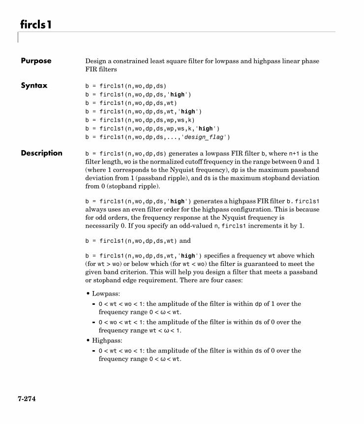
fircls1
7fircls1Purpose Design a constrained least square filter for lowpass and highpass linear phase FIR filters
Syntax b = fircls1(n,wo,dp,ds)b = fircls1(n,wo,dp,ds,'high')b = fircls1(n,wo,dp,ds,wt)b = fircls1(n,wo,dp,ds,wt,'high')b = fircls1(n,wo,dp,ds,wp,ws,k)b = fircls1(n,wo,dp,ds,wp,ws,k,'high')b = fircls1(n,wo,dp,ds,...,'design_flag')
Description b = fircls1(n,wo,dp,ds) generates a lowpass FIR filter b, where n+1 is the filter length, wo is the normalized cutoff frequency in the range between 0 and 1 (where 1 corresponds to the Nyquist frequency), dp is the maximum passband deviation from 1 (passband ripple), and ds is the maximum stopband deviation from 0 (stopband ripple).
b = fircls1(n,wo,dp,ds,'high') generates a highpass FIR filter b. fircls1 always uses an even filter order for the highpass configuration. This is because for odd orders, the frequency response at the Nyquist frequency is necessarily 0. If you specify an odd-valued n, fircls1 increments it by 1.
b = fircls1(n,wo,dp,ds,wt) and
b = fircls1(n,wo,dp,ds,wt,'high') specifies a frequency wt above which (for wt > wo) or below which (for wt < wo) the filter is guaranteed to meet the given band criterion. This will help you design a filter that meets a passband or stopband edge requirement. There are four cases:
• Lowpass:
- 0 < wt < wo < 1: the amplitude of the filter is within dp of 1 over the frequency range 0 < ω < wt.
- 0 < wo < wt < 1: the amplitude of the filter is within ds of 0 over the frequency range wt < ω < 1.
• Highpass:
- 0 < wt < wo < 1: the amplitude of the filter is within ds of 0 over the frequency range 0 < ω < wt.
7-274
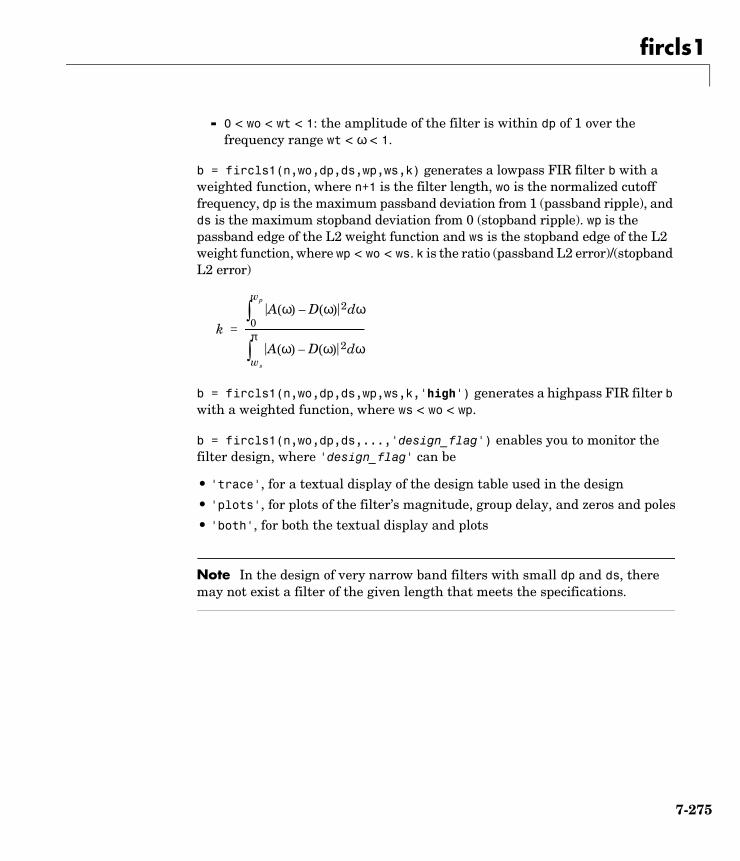
fircls1
- 0 < wo < wt < 1: the amplitude of the filter is within dp of 1 over the frequency range wt < ω < 1.
b = fircls1(n,wo,dp,ds,wp,ws,k) generates a lowpass FIR filter b with a weighted function, where n+1 is the filter length, wo is the normalized cutoff frequency, dp is the maximum passband deviation from 1 (passband ripple), and ds is the maximum stopband deviation from 0 (stopband ripple). wp is the passband edge of the L2 weight function and ws is the stopband edge of the L2 weight function, where wp < wo < ws. k is the ratio (passband L2 error)/(stopband L2 error)
b = fircls1(n,wo,dp,ds,wp,ws,k,'high') generates a highpass FIR filter b with a weighted function, where ws < wo < wp.
b = fircls1(n,wo,dp,ds,...,'design_flag') enables you to monitor the filter design, where 'design_flag' can be
• 'trace', for a textual display of the design table used in the design
• 'plots', for plots of the filter’s magnitude, group delay, and zeros and poles
• 'both', for both the textual display and plots
Note In the design of very narrow band filters with small dp and ds, there may not exist a filter of the given length that meets the specifications.
kA ω( ) D ω( )– 2 ωd
0
wp
∫
A ω( ) D ω( )– 2 ωdws
π
∫------------------------------------------------------=
7-275
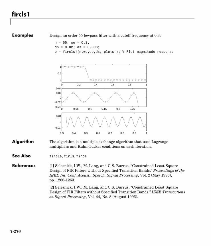
fircls1
Examples Design an order 55 lowpass filter with a cutoff frequency at 0.3:
n = 55; wo = 0.3;dp = 0.02; ds = 0.008;b = fircls1(n,wo,dp,ds,'plots'); % Plot magnitude response
Algorithm The algorithm is a multiple exchange algorithm that uses Lagrange multipliers and Kuhn-Tucker conditions on each iteration.
See Also fircls, firls, firpm
References [1] Selesnick, I.W., M. Lang, and C.S. Burrus, “Constrained Least Square Design of FIR Filters without Specified Transition Bands,” Proceedings of the IEEE Int. Conf. Acoust., Speech, Signal Processing, Vol. 2 (May 1995), pp. 1260-1263.
[2] Selesnick, I.W., M. Lang, and C.S. Burrus, “Constrained Least Square Design of FIR Filters without Specified Transition Bands,” IEEE Transactions on Signal Processing, Vol. 44, No. 8 (August 1996).
0 0.2 0.4 0.6 0.8 1
0
0.5
1
0 0.05 0.1 0.15 0.2 0.25-0.04
-0.02
0
0.02
0.04
0.3 0.4 0.5 0.6 0.7 0.8 0.9 1
-0.01
0
0.01
7-276
firgauss
7firgaussPurpose Design a FIR Gaussian digital filter
Syntax b = firgauss(k,n)[b,n] = firgauss(k,'minorder',v)
Description Gaussian filters are important in many signal processing, image processing, and communication applications. These filters are characterized by narrow bandwidths, sharp cutoffs, and low overshoots. A key feature of Gaussian filters is that the Fourier transform of a Gaussian is also a Gaussian, so the filter has the same response shape in both the time and frequency domains.
b = firgauss(k,n) returns an FIR filter whose impulse response approximates an ideal zero-mean Gaussian. Filters with this type of impulse response act as lowpass filters. The implementation of this filter is a cascade of k boxcar (uniform-coefficient) filters of integer length n. Increasing the number of cascades, k, or the length of each boxcar, n, produces a closer approximation to an ideal Gaussian. The filter is returned in vector b.
A 1-D Gaussian or Normal density function is defined as
where , σ is the standard deviation, and µ is the mean.
A measure of how well a lowpass filter rejects frequencies outside its passband is the ratio of the highest sidelobe level (HSSL) to the DC response . For firgauss, the HSSL is approximately -13.3 dB * k, where k is the number of cascaded filters, so for a cascade of four boxcars, the HSSL is -53 dB.
[b,n] = firgauss(k,'minorder',v) returns a Gaussian filter with variance, v. The variance is the sum of the variances of the convolutions (cascades) of the individual boxcar filters. Note that it is not the variance of the filter’s frequency response. The required 'minorder' flag causes firgauss to use the minimum length, n, to achieve the overall variance. When k >= 4, firgauss uses an optimization to determine the minimum length for each of the boxcar filters. This optimization produces an approximation to the ideal Gaussian impulse response that is minimal in the root mean square (rms) sense.
g x( ) 1σ 2π---------------e x µ–( )– 2 2σ⁄ 2
=
∞– x ∞≤ ≤
7-277
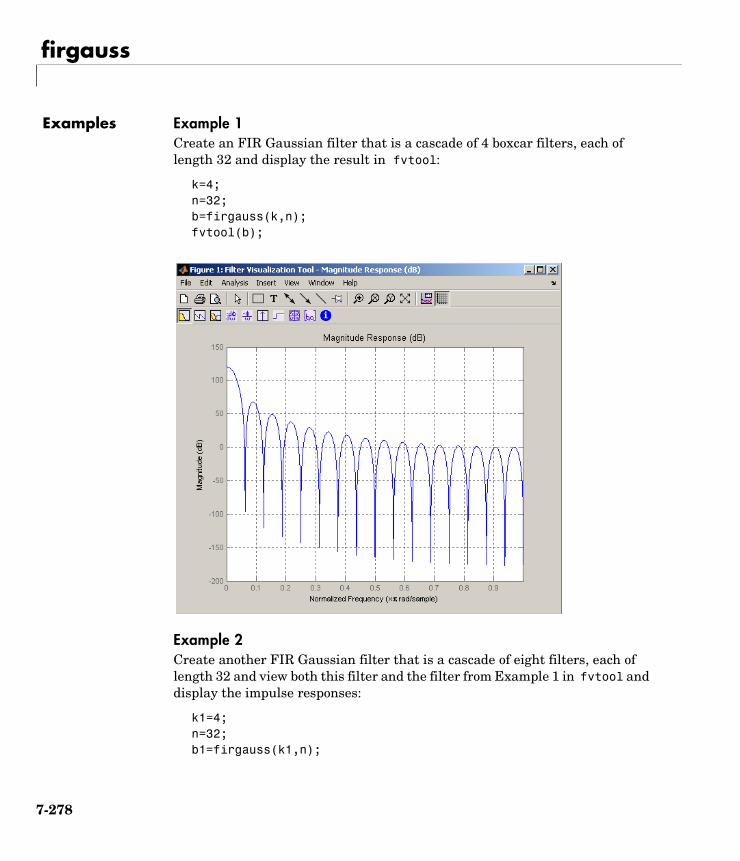
firgauss
Examples Example 1Create an FIR Gaussian filter that is a cascade of 4 boxcar filters, each of length 32 and display the result in fvtool:
k=4;n=32;b=firgauss(k,n);fvtool(b);
Example 2Create another FIR Gaussian filter that is a cascade of eight filters, each of length 32 and view both this filter and the filter from Example 1 in fvtool and display the impulse responses:
k1=4;n=32;b1=firgauss(k1,n);
7-278
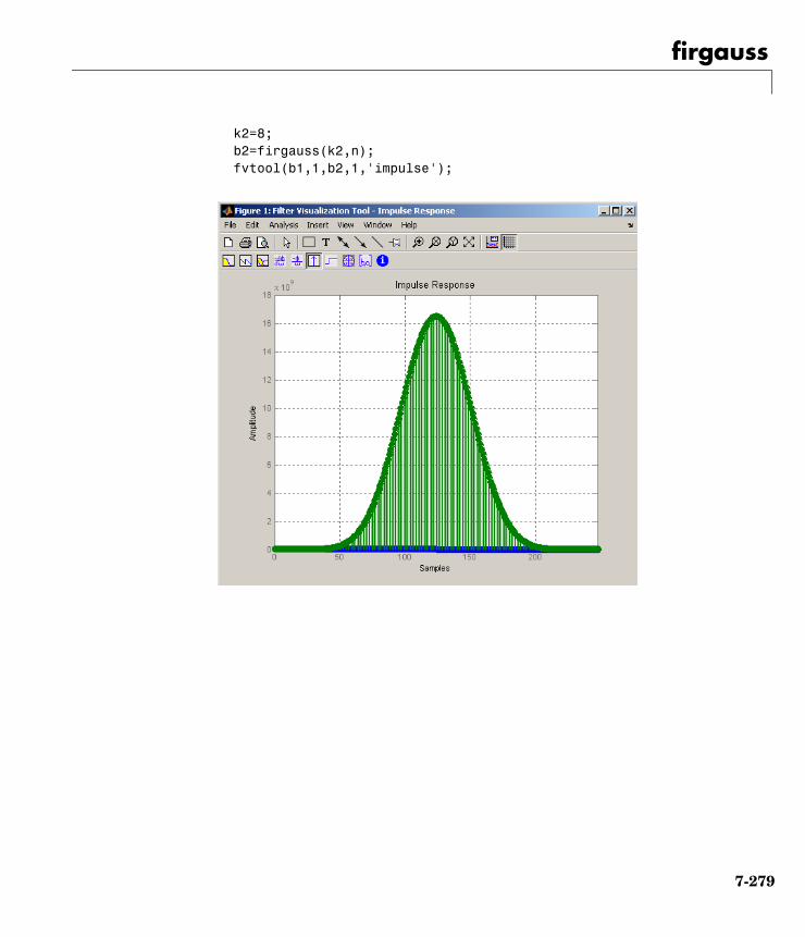
firgauss
k2=8;b2=firgauss(k2,n);fvtool(b1,1,b2,1,'impulse');
7-279
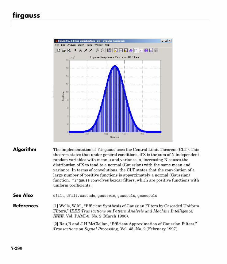
firgauss
Algorithm The implementation of firgauss uses the Central Limit Theorem (CLT). This theorem states that under general conditions, if X is the sum of N independent random variables with mean µ and variance σ, increasing N causes the distribution of X to tend to a normal (Gaussian) with the same mean and variance. In terms of convolutions, the CLT states that the convolution of a large number of positive functions is apporximately a normal (Gaussian) function. firgauss convolves boxcar filters, which are positive functions with uniform coefficients.
See Also dfilt, dfilt.cascade, gausswin, gauspuls, gmonopuls
References [1] Wells, W.M., “Efficient Synthesis of Gaussian Filters by Cascaded Uniform Filters,” IEEE Transactions on Pattern Analysis and Machine Intelligence, IEEE. Vol. PAMI-8, No. 2 (March 1986).
[2] Rau,R and J.H.McClellan, “Efficient Approximation of Gaussian Filters,” Transactions on Signal Processing, Vol. 45, No. 2 (February 1997).
7-280

firgauss
[3] Papoulis, A, Probability, Random Variables and Stochastic Processes, McGraw-Hill, 1991, pp. 214-215.
7-281
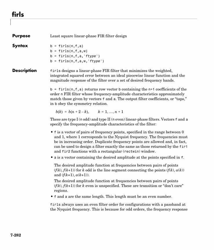
firls
7firlsPurpose Least square linear-phase FIR filter design
Syntax b = firls(n,f,a)b = firls(n,f,a,w)b = firls(n,f,a,'ftype')b = firls(n,f,a,w,'ftype')
Description firls designs a linear-phase FIR filter that minimizes the weighted, integrated squared error between an ideal piecewise linear function and the magnitude response of the filter over a set of desired frequency bands.
b = firls(n,f,a) returns row vector b containing the n+1 coefficients of the order n FIR filter whose frequency-amplitude characteristics approximately match those given by vectors f and a. The output filter coefficients, or “taps,” in b obey the symmetry relation.
These are type I (n odd) and type II (n even) linear-phase filters. Vectors f and a specify the frequency-amplitude characteristics of the filter:
• f is a vector of pairs of frequency points, specified in the range between 0 and 1, where 1 corresponds to the Nyquist frequency. The frequencies must be in increasing order. Duplicate frequency points are allowed and, in fact, can be used to design a filter exactly the same as those returned by the fir1 and fir2 functions with a rectangular (rectwin) window.
• a is a vector containing the desired amplitude at the points specified in f.
The desired amplitude function at frequencies between pairs of points (f(k), f(k+1)) for k odd is the line segment connecting the points (f(k), a(k)) and (f(k+1), a(k+1)).
The desired amplitude function at frequencies between pairs of points (f(k), f(k+1)) for k even is unspecified. These are transition or “don’t care” regions.
• f and a are the same length. This length must be an even number.
firls always uses an even filter order for configurations with a passband at the Nyquist frequency. This is because for odd orders, the frequency response
b k( ) b n 2 k–+( ) k 1= … n 1+, , ,=
7-282
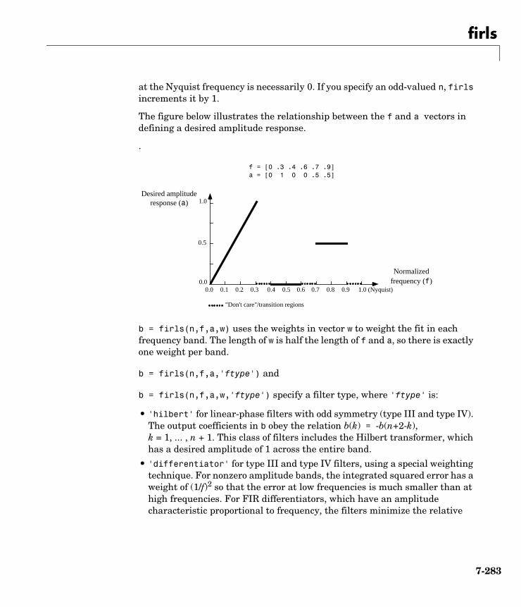
firls
at the Nyquist frequency is necessarily 0. If you specify an odd-valued n, firls increments it by 1.
The figure below illustrates the relationship between the f and a vectors in defining a desired amplitude response.
.
b = firls(n,f,a,w) uses the weights in vector w to weight the fit in each frequency band. The length of w is half the length of f and a, so there is exactly one weight per band.
b = firls(n,f,a,'ftype') and
b = firls(n,f,a,w,'ftype') specify a filter type, where 'ftype' is:
• 'hilbert' for linear-phase filters with odd symmetry (type III and type IV). The output coefficients in b obey the relation b(k) = -b(n+2-k), k = 1, ... , n + 1. This class of filters includes the Hilbert transformer, which has a desired amplitude of 1 across the entire band.
• 'differentiator' for type III and type IV filters, using a special weighting technique. For nonzero amplitude bands, the integrated squared error has a weight of (1/f)2 so that the error at low frequencies is much smaller than at high frequencies. For FIR differentiators, which have an amplitude characteristic proportional to frequency, the filters minimize the relative
1.0
0.0
Desired amplituderesponse (a)
Normalizedfrequency (f)
0.5
"Don't care"/transition regions
f = [0 .3 .4 .6 .7 .9]a = [0 1 0 0 .5 .5]
0.1 0.2 0.3 0.4 0.5 0.6 0.70.0 0.8 0.9 1.0 (Nyquist)
7-283
firls
integrated squared error (the integral of the square of the ratio of the error to the desired amplitude).
Examples Example 1Design an order 255 lowpass filter with transition band:
b = firls(255,[0 0.25 0.3 1],[1 1 0 0]);
Example 2Design a 31 coefficient differentiator:
b = firls(30,[0 0.9],[0 0.9],'differentiator');
Example 3Design a 24th-order anti-symmetric filter with piecewise linear passbands and plot the desired and actual frequency response:
F = [0 0.3 0.4 0.6 0.7 0.9]; A = [0 1 0 0 0.5 0.5];b = firls(24,F,A,'hilbert');for i=1:2:6, plot([F(i) F(i+1)],[A(i) A(i+1)],'--'), hold onend[H,f] = freqz(b,1,512,2);plot(f,abs(H)), grid on, hold offlegend('Ideal','firls Design')
7-284
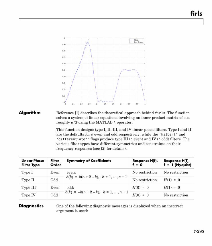
firls
Algorithm Reference [1] describes the theoretical approach behind firls. The function solves a system of linear equations involving an inner product matrix of size roughly n/2 using the MATLAB \ operator.
This function designs type I, II, III, and IV linear-phase filters. Type I and II are the defaults for n even and odd respectively, while the 'hilbert' and 'differentiator' flags produce type III (n even) and IV (n odd) filters. The various filter types have different symmetries and constraints on their frequency responses (see [2] for details).
Diagnostics One of the following diagnostic messages is displayed when an incorrect argument is used:
0 0.1 0.2 0.3 0.4 0.5 0.6 0.7 0.8 0.9 10
0.1
0.2
0.3
0.4
0.5
0.6
0.7
0.8
0.9
1Ideal firls Design
Linear Phase Filter Type
Filter Order
Symmetry of Coefficients Response H(f), f = 0
Response H(f), f = 1 (Nyquist)
Type I Even even: No restriction No restriction
Type II Odd No restriction H(1) = 0
Type III Even odd: H(0) = 0 H(1) = 0
Type IV Odd H(0) = 0 No restriction
b k( ) b n 2 k–+( ) k 1= … n 1+, , ,=
b k( ) b– n 2 k–+( ) k 1= … n 1+, , ,=
7-285
firls
F must be even length.F and A must be equal lengths.Requires symmetry to be 'hilbert' or 'differentiator'.Requires one weight per band.Frequencies in F must be nondecreasing.Frequencies in F must be in range [0,1].
A more serious warning message is
Warning: Matrix is close to singular or badly scaled.
This tends to happen when the product of the filter length and transition width grows large. In this case, the filter coefficients b might not represent the desired filter. You can check the filter by looking at its frequency response.
See Also fir1, fir2, firrcos, firpm
References [1] Parks, T.W., and C.S. Burrus, Digital Filter Design, John Wiley & Sons, 1987, pp. 54-83.
[2] Oppenheim, A.V., and R.W. Schafer, Discrete-Time Signal Processing, Prentice-Hall, 1989, pp. 256-266.
7-286
firpm
7firpmPurpose Compute the Parks-McClellan optimal FIR filter design
Syntax b = firpm(n,f,a)b = firpm(n,f,a,w)b = firpm(n,f,a,'ftype')b = firpm(n,f,a,w,'ftype')b = firpm(...,lgrid)b = firpm(n,f,'fresp',w)b = firpm(n,f,'fresp',w,'ftype')b = firpm(n,f,'fresp',p1,p2,...,w)b = firpm(n,f,'fresp',p1,p2,...,w,'ftype')[b,delta] = firpm(...)[b,delta,opt] = firpm(...)
Description firpm designs a linear-phase FIR filter using the Parks-McClellan algorithm [1]. The Parks-McClellan algorithm uses the firpm exchange algorithm and Chebyshev approximation theory to design filters with an optimal fit between the desired and actual frequency responses. The filters are optimal in the sense that the maximum error between the desired frequency response and the actual frequency response is minimized. Filters designed this way exhibit an equiripple behavior in their frequency responses and are sometimes called equiripple filters. firpm exhibits discontinuities at the head and tail of its impulse response due to this equiripple nature.
b = firpm(n,f,a) returns row vector b containing the n+1 coefficients of the order n FIR filter whose frequency-amplitude characteristics match those given by vectors f and a.
The output filter coefficients (taps) in b obey the symmetry relation:
b k( ) b n 2 k–+( ) k 1= … n 1+, , ,=
7-287
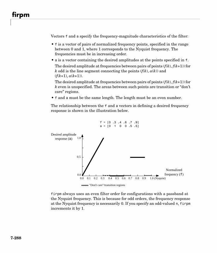
firpm
Vectors f and a specify the frequency-magnitude characteristics of the filter:
• f is a vector of pairs of normalized frequency points, specified in the range between 0 and 1, where 1 corresponds to the Nyquist frequency. The frequencies must be in increasing order.
• a is a vector containing the desired amplitudes at the points specified in f.
The desired amplitude at frequencies between pairs of points (f(k), f(k+1)) for k odd is the line segment connecting the points (f(k), a(k)) and (f(k+1), a(k+1)).
The desired amplitude at frequencies between pairs of points (f(k), f(k+1)) for k even is unspecified. The areas between such points are transition or “don’t care” regions.
• f and a must be the same length. The length must be an even number.
The relationship between the f and a vectors in defining a desired frequency response is shown in the illustration below.
firpm always uses an even filter order for configurations with a passband at the Nyquist frequency. This is because for odd orders, the frequency response at the Nyquist frequency is necessarily 0. If you specify an odd-valued n, firpm increments it by 1.
1.0
0.0
Desired amplituderesponse (a)
Normalizedfrequency (f)
0.5
"Don't care"/transition regions
f = [0 .3 .4 .6 .7 .9]a = [0 1 0 0 .5 .5]
0.1 0.2 0.3 0.4 0.5 0.6 0.70.0 0.8 0.9 1.0 (Nyquist)
7-288
firpm
firpm(n,f,a,w) uses the weights in vector w to weight the fit in each frequency band. The length of w is half the length of f and a, so there is exactly one weight per band.
b = firpm(n,f,a,'ftype') and
b = firpm(n,f,a,w,'ftype') specify a filter type, where 'ftype' is
• 'hilbert', for linear-phase filters with odd symmetry (type III and type IV)
The output coefficients in b obey the relation b(k) = -b(n+2-k), k = 1, ..., n + 1. This class of filters includes the Hilbert transformer, which has a desired amplitude of 1 across the entire band.
For example, h = firpm(30,[0.1 0.9],[1 1],'hilbert');
designs an approximate FIR Hilbert transformer of length 31.
• 'differentiator', for type III and type IV filters, using a special weighting technique
For nonzero amplitude bands, it weights the error by a factor of 1/f so that the error at low frequencies is much smaller than at high frequencies. For FIR differentiators, which have an amplitude characteristic proportional to frequency, these filters minimize the maximum relative error (the maximum of the ratio of the error to the desired amplitude).
b = firpm(...,lgrid) uses the integer lgrid to control the density of the frequency grid, which has roughly (lgrid*n)/(2*bw) frequency points, where bw is the fraction of the total frequency band interval [0,1] covered by f. Increasing lgrid often results in filters that more exactly match an equiripple filter, but that take longer to compute. The default value of 16 is the minimum value that should be specified for lgrid. Note that the lgrid argument must be a 1-by-1 cell array.
b = firpm(n,f,'fresp',w) returns row vector b containing the n+1 coefficients of the order n FIR filter whose frequency-amplitude characteristics best approximate the response specified by function fresp. The function is called from within firpm with the following syntax.
[dh,dw] = fresp(n,f,gf,w)
7-289
firpm
The arguments are similar to those for firpm:
• n is the filter order.
• f is the vector of normalized frequency band edges that appear monotonically between 0 and 1, where 1 is the Nyquist frequency.
• gf is a vector of grid points that have been linearly interpolated over each specified frequency band by firpm. gf determines the frequency grid at which the response function must be evaluated, and contains the same data returned by cfirpm in the fgrid field of the opt structure.
• w is a vector of real, positive weights, one per band, used during optimization. w is optional in the call to firpm; if not specified, it is set to unity weighting before being passed to fresp.
• dh and dw are the desired complex frequency response and band weight vectors, respectively, evaluated at each frequency in grid gf.
The predefined frequency response function fresp that firpm calls is remezfrf in the signal/private directory.
b = firpm(n,f,'fresp',p1,p2,...,w) allows you to specify additional parameters (p1, p2, etc.) to pass to fresp. Note that b = firpm(n,f,a,w) is a synonym for b = firpm(n,f,'firpmfrf',a,w), where a is a vector containing the desired amplitudes at the points specified in f.
b = firpm(n,f,'fresp',w,'ftype') and
b = firpm(n,f,'fresp',p1,p2,...,w,'ftype') design antisymmetric (odd) rather than symmetric (even) filters, where 'ftype' is either 'd' for a differentiator or 'h' for a Hilbert transformer.
In the absence of a specification for ftype, a preliminary call is made to fresp to determine the default symmetry property sym. This call is made using the syntax.
sym = fresp('defaults',n,f,[],w,p1,p2,...)
The arguments n, f, w, etc., may be used as necessary in determining an appropriate value for sym, which firpm expects to be either 'even' or 'odd'. If the fresp function does not support this calling syntax, firpm defaults to even symmetry.
7-290
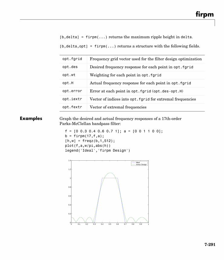
firpm
[b,delta] = firpm(...) returns the maximum ripple height in delta.
[b,delta,opt] = firpm(...) returns a structure with the following fields.
Examples Graph the desired and actual frequency responses of a 17th-order Parks-McClellan bandpass filter:
f = [0 0.3 0.4 0.6 0.7 1]; a = [0 0 1 1 0 0];b = firpm(17,f,a);[h,w] = freqz(b,1,512);plot(f,a,w/pi,abs(h))legend('Ideal','firpm Design')
opt.fgrid Frequency grid vector used for the filter design optimization
opt.des Desired frequency response for each point in opt.fgrid
opt.wt Weighting for each point in opt.fgrid
opt.H Actual frequency response for each point in opt.fgrid
opt.error Error at each point in opt.fgrid (opt.des-opt.H)
opt.iextr Vector of indices into opt.fgrid for extremal frequencies
opt.fextr Vector of extremal frequencies
0 0.1 0.2 0.3 0.4 0.5 0.6 0.7 0.8 0.9 10
0.2
0.4
0.6
0.8
1
1.2
1.4Ideal remez Design
7-291
firpm
Algorithm firpm is a MEX-file version of the original Fortran code from [1], altered to design arbitrarily long filters with arbitrarily many linear bands.
firpm designs type I, II, III, and IV linear-phase filters. Type I and type II are the defaults for n even and n odd, respectively, while type III (n even) and type IV (n odd) are obtained with the 'hilbert' and 'differentiator' flags. The different types of filters have different symmetries and certain constraints on their frequency responses (see [5] for more details).
Diagnostics If you get the following warning message,
- Failure to Converge -Probable cause is machine rounding error.
it is possible that the filter design may still be correct. Verify the design by checking its frequency response.
See Also butter, cheby1, cheby2, cfirpm, ellip, fir1, fir2, fircls, fircls1, firls, firrcos, firgr, firpmord, yulewalk
References [1] Programs for Digital Signal Processing, IEEE Press, New York, 1979, Algorithm 5.1.
[2] Selected Papers in Digital Signal Processing, II, IEEE Press, New York, 1979.
[3] Parks, T.W., and C.S. Burrus, Digital Filter Design, John Wiley & Sons, New York:, 1987, p. 83.
Linear Phase Filter Type
Filter Order
Symmetry of Coefficients Response H(f), f = 0
Response H(f), f = 1 (Nyquist)
Type I Even even: No restriction No restriction
Type II Odd No restriction H(1) = 0
Type III Even odd: H(0) = 0 H(1) = 0
Type IV Odd H(0) = 0 No restriction
b k( ) b n 2 k–+( ) k 1= … n 1+, , ,=
b k( ) b– n 2 k–+( ) k 1= … n 1+, , ,=
7-292

firpm
[4] Rabiner, L.R., J.H. McClellan, and T.W. Parks, “FIR Digital Filter Design Techniques Using Weighted Chebyshev Approximations,” Proc. IEEE 63 (1975).
[5] Oppenheim, A.V., and R.W. Schafer, Discrete-Time Signal Processing, Prentice-Hall, Englewood Cliffs, NJ, 1989, pp. 256-266.
7-293
firpmord
7firpmordPurpose Parks-McClellan optimal FIR filter order estimation
Syntax [n,fo,ao,w] = firpmord(f,a,dev)[n,fo,ao,w] = firpmord(f,a,dev,fs)c = firpmord(f,a,dev,fs,'cell')
Description [n,fo,ao,w] = firpmord(f,a,dev) finds the approximate order, normalized frequency band edges, frequency band amplitudes, and weights that meet input specifications f, a, and dev.
• f is a vector of frequency band edges (between 0 and fs/2, where fs is the sampling frequency), and a is a vector specifying the desired amplitude on the bands defined by f. The length of f is two less than twice the length of a. The desired function is piecewise constant.
• dev is a vector the same size as a that specifies the maximum allowable deviation or ripples between the frequency response and the desired amplitude of the output filter for each band.
Use firpm with the resulting order n, frequency vector fo, amplitude response vector ao, and weights w to design the filter b which approximately meets the specifications given by firpmord input parameters f, a, and dev.
b = firpm(n,fo,ao,w)
[n,fo,ao,w] = firpmord(f,a,dev,fs) specifies a sampling frequency fs. fs defaults to 2 Hz, implying a Nyquist frequency of 1 Hz. You can therefore specify band edges scaled to a particular application’s sampling frequency.
In some cases firpmord underestimates the order n. If the filter does not meet the specifications, try a higher order such as n+1 or n+2.
c = firpmord(f,a,dev,fs,'cell') generates a cell-array whose elements are the parameters to firpm.
Examples Example 1Design a minimum-order lowpass filter with a 500 Hz passband cutoff frequency and 600 Hz stopband cutoff frequency, with a sampling frequency of 2000 Hz, at least 40 dB attenuation in the stopband, and less than 3 dB of ripple in the passband:
7-294
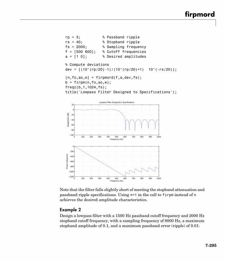
firpmord
rp = 3; % Passband ripplers = 40; % Stopband ripplefs = 2000; % Sampling frequencyf = [500 600]; % Cutoff frequenciesa = [1 0]; % Desired amplitudes
% Compute deviationsdev = [(10^(rp/20)-1)/(10^(rp/20)+1) 10^(-rs/20)];
[n,fo,ao,w] = firpmord(f,a,dev,fs);b = firpm(n,fo,ao,w);freqz(b,1,1024,fs);title('Lowpass Filter Designed to Specifications');
Note that the filter falls slightly short of meeting the stopband attenuation and passband ripple specifications. Using n+1 in the call to firpm instead of n achieves the desired amplitude characteristics.
Example 2Design a lowpass filter with a 1500 Hz passband cutoff frequency and 2000 Hz stopband cutoff frequency, with a sampling frequency of 8000 Hz, a maximum stopband amplitude of 0.1, and a maximum passband error (ripple) of 0.01:
0 100 200 300 400 500 600 700 800 900 1000−1200
−1000
−800
−600
−400
−200
0
Frequency (Hz)
Ph
ase
(d
eg
ree
s)
0 100 200 300 400 500 600 700 800 900 1000−100
−80
−60
−40
−20
0
20
Frequency (Hz)
Ma
gn
itud
e (
dB
)
Lowpass Filter Designed to Specifications
7-295
firpmord
[n,fo,ao,w] = firpmord([1500 2000],[1 0],[0.01 0.1],8000 );b = firpm(n,fo,ao,w);
This is equivalent to
c = firpmord( [1500 2000],[1 0],[0.01 0.1],8000,'cell');b = firpm(c:);
Note In some cases, firpmord underestimates or overestimates the order n. If the filter does not meet the specifications, try a higher order such as n+1 or n+2.
Results are inaccurate if the cutoff frequencies are near 0 or the Nyquist frequency.
Algorithm firpmord uses the algorithm suggested in [1]. This method is inaccurate for band edges close to either 0 or the Nyquist frequency (fs/2).
See Also buttord, cheb1ord, cheb2ord, ellipord, kaiserord, firpm
References [1] Rabiner, L.R., and O. Herrmann, “The Predictability of Certain Optimum Finite Impulse Response Digital Filters,” IEEE Trans. on Circuit Theory, Vol. CT-20, No. 4 (July 1973), pp. 401-408.
[2] Rabiner, L.R., and B. Gold. Theory and Application of Digital Signal Processing. Englewood Cliffs, NJ: Prentice-Hall, 1975, pp. 156-157.
7-296
firrcos
7firrcosPurpose Raised cosine FIR filter design
Syntax b = firrcos(n,F0,df,fs)b = firrcos(n,F0,df,fs,'bandwidth')b = firrcos(n,F0,df)b = firrcos(n,F0,r,fs,'rolloff')b = firrcos(...,'type')b = firrcos(...,'type',delay)b = firrcos(...,'type',delay,window)[b,a] = firrcos(...)
Description b = firrcos(n,F0,df,fs) or, equivalently,
b = firrcos(n,F0,df,fs,'bandwidth') returns an order n lowpass linear-phase FIR filter with a raised cosine transition band. The filter has cutoff frequency F0, transition bandwidth df, and sampling frequency fs, all in hertz. df must be small enough so that F0 ± df/2 is between 0 and fs/2. The coefficients in b are normalized so that the nominal passband gain is always equal to 1. Specify fs as the empty vector [] to use the default value fs = 2.
b = firrcos(n,F0,df) uses a default sampling frequency of fs = 2.
b = firrcos(n,F0,r,fs,'rolloff') interprets the third argument, r, as the rolloff factor instead of the transition bandwidth, df. r must be in the range [0,1].
b = firrcos(...,'type') designs either a normal raised cosine filter or a square root raised cosine filter according to how you specify of the string 'type'. Specify 'type' as:
• 'normal', for a regular raised cosine filter. This is the default, and is also in effect when the 'type' argument is left empty, [].
• 'sqrt', for a square root raised cosine filter.
b = firrcos(...,'type',delay) specifies an integer delay in the range [0,n+1]. The default is n/2 for even n and (n+1)/2 for odd n.
b = firrcos(...,'type',delay,window) applies a length n+1 window to the designed filter to reduce the ripple in the frequency response. window must be
7-297
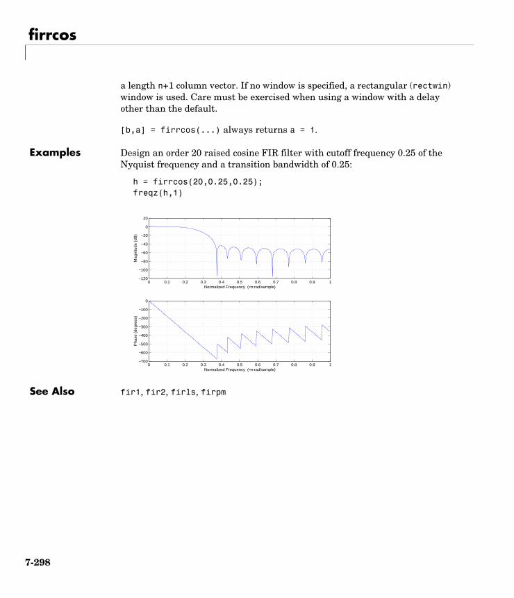
firrcos
a length n+1 column vector. If no window is specified, a rectangular (rectwin) window is used. Care must be exercised when using a window with a delay other than the default.
[b,a] = firrcos(...) always returns a = 1.
Examples Design an order 20 raised cosine FIR filter with cutoff frequency 0.25 of the Nyquist frequency and a transition bandwidth of 0.25:
h = firrcos(20,0.25,0.25);freqz(h,1)
See Also fir1, fir2, firls, firpm
0 0.1 0.2 0.3 0.4 0.5 0.6 0.7 0.8 0.9 1−700
−600
−500
−400
−300
−200
−100
0
Normalized Frequency (×π rad/sample)
Pha
se (
degr
ees)
0 0.1 0.2 0.3 0.4 0.5 0.6 0.7 0.8 0.9 1−120
−100
−80
−60
−40
−20
0
20
Normalized Frequency (×π rad/sample)
Mag
nitu
de (
dB)
7-298
flattopwin
7flattopwinPurpose Compute a Flat Top weighted window.
Syntax w = flattopwin(n)w = flattopwin(n,'sflag')
Description Flat Top windows have very low passband ripple (< 0.01 dB) and are used primarily for calibration purposes. Their bandwidth is approximately 2.5 times wider than a Hann window.
w = flattopwin(n) returns the n-point symmetric Flat Top window in column vector w.
w = flattopwin(n,sflag) returns the n-point symmetric Flat Top window using sflag window sampling, where sflag is either 'symmetric' or 'periodic'.
Algorithm Flat top windows are summations of cosines. The coefficients of a flat top window are computed from the following equation
where and elsewhere.
Examples Create a 64-point, symmetric Flat Top window and view the window using WVTool:
w = flattopwin(64); wvtool(w);
w t( ) 1 1.93 2πtT
--------- 1.29 4πt
T--------- 0.388 6πt
T--------- 0.0322 8πt
T--------- cos+cos–cos+cos–=
0 t T≤ ≤ w t( ) 0=
7-299
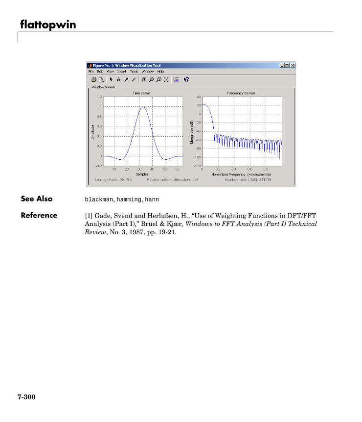
flattopwin
See Also blackman, hamming, hann
Reference [1] Gade, Svend and Herlufsen, H., “Use of Weighting Functions in DFT/FFT Analysis (Part I),” Brüel & Kjær, Windows to FFT Analysis (Part I) Technical Review, No. 3, 1987, pp. 19-21.
7-300
freqs
7freqsPurpose Frequency response of analog filters
Syntax h = freqs(b,a,w)[h,w] = freqs(b,a)[h,w] = freqs(b,a,f)freqs(b,a)
Description freqs returns the complex frequency response H(jω) (Laplace transform) of an analog filter
given the numerator and denominator coefficients in vectors b and a.
h = freqs(b,a,w) returns the complex frequency response of the analog filter specified by coefficient vectors b and a. freqs evaluates the frequency response along the imaginary axis in the complex plane at the angular frequencies in rad/sec specified in real vector w, which must contain more than one frequency.
[h,w] = freqs(b,a) automatically picks a set of 200 frequency points w on which to compute the frequency response h.
[h,w] = freqs(b,a,f) picks f number of frequencies on which to compute the frequency response h.
freqs with no output arguments plots the magnitude and phase response versus frequency in the current figure window.
freqs works only for real input systems and positive frequencies.
Examples Find and graph the frequency response of the transfer function given by:
a = [1 0.4 1];b = [0.2 0.3 1];w = logspace(-1,1);freqs(b,a,w)
H s( )B s( )A s( )----------- b 1( )sn b 2( )sn 1– b n 1+( )+ + +
a 1( )sm a 2( )sm 1– a m 1+( )+ + +-------------------------------------------------------------------------------------------= =
H s( )0.2s2 0.3s 1+ +
s2 0.4s 1+ +-----------------------------------------=
7-301
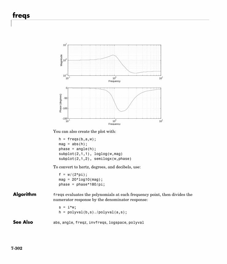
freqs
You can also create the plot with:
h = freqs(b,a,w);mag = abs(h);phase = angle(h);subplot(2,1,1), loglog(w,mag)subplot(2,1,2), semilogx(w,phase)
To convert to hertz, degrees, and decibels, use:
f = w/(2*pi);mag = 20*log10(mag);phase = phase*180/pi;
Algorithm freqs evaluates the polynomials at each frequency point, then divides the numerator response by the denominator response:
s = i*w;h = polyval(b,s)./polyval(a,s);
See Also abs, angle, freqz, invfreqs, logspace, polyval
10-1
100
101
10-1
100
101
Frequency
Mag
nitu
de
10-1
100
101
-150
-100
-50
0
Frequency
Pha
se (
degr
ees)
7-302

freqspace
7freqspacePurpose Frequency spacing for frequency response
freqspace is a MATLAB function.
7-303
freqz
7freqzPurpose Compute the frequency response of digital filters
Syntax [h,w]= freqz(b,a,l)h = freqz(b,a,w)[h,w] = freqz(b,a,l,'whole')[h,f] = freqz(b,a,l,fs)h = freqz(b,a,f,fs)[h,f] = freqz(b,a,l,'whole',fs)freqz(b,a,...)freqz(Hd)
Description [h,w] = freqz(b,a,l) returns the frequency response vector h and the corresponding angular frequency vector w for the digital filter whose transfer function is determined by the (real or complex) numerator and denominator polynomials represented in the vectors b and a, respectively. The vectors h and w are both of length l. The angular frequency vector w has values ranging from 0 to π radians per sample. When you don’t specify the integer l, or you specify it as the empty vector [], the frequency response is calculated using the default value of 512 samples.
h = freqz(b,a,w) returns the frequency response vector h calculated at the frequencies (in radians per sample) supplied by the vector w. The vector w can have any length.
[h,w] = freqz(b,a,l,'whole') uses n sample points around the entire unit circle to calculate the frequency response. The frequency vector w has length l and has values ranging from 0 to 2π radians per sample.
[h,f] = freqz(b,a,l,fs) returns the frequency response vector h and the corresponding frequency vector f for the digital filter whose transfer function is determined by the (real or complex) numerator and denominator polynomials represented in the vectors b and a, respectively. The vectors h and f are both of length l. For this syntax, the frequency response is calculated using the sampling frequency specified by the scalar fs (in hertz). The frequency vector f is calculated in units of hertz (Hz). The frequency vector f has values ranging from 0 to fs/2 Hz.
7-304
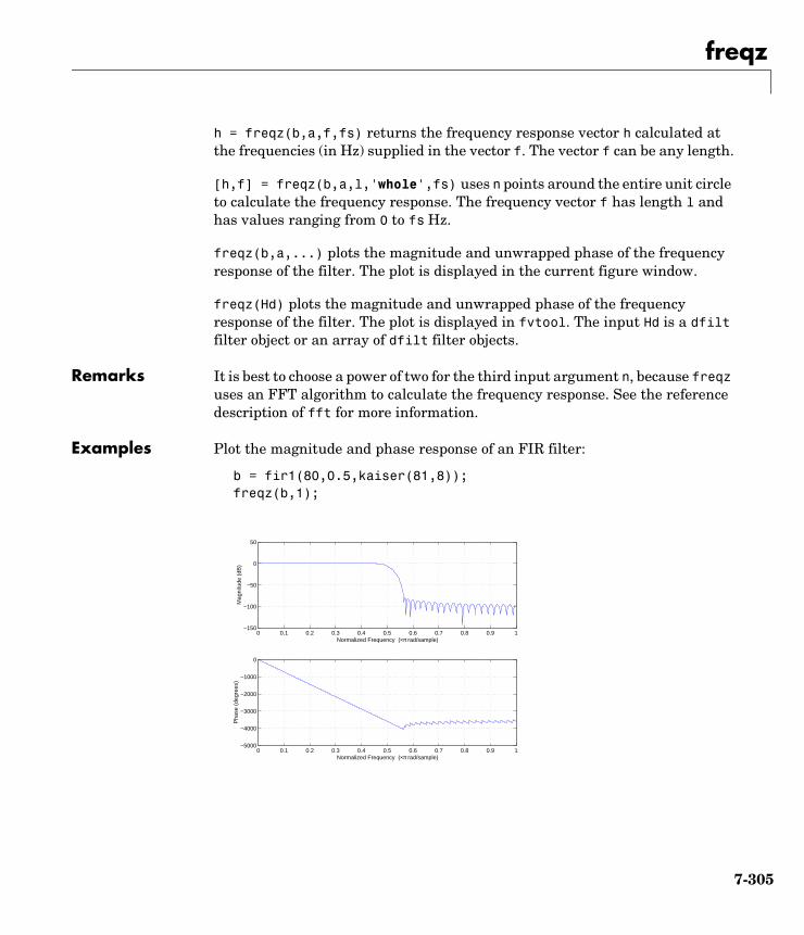
freqz
h = freqz(b,a,f,fs) returns the frequency response vector h calculated at the frequencies (in Hz) supplied in the vector f. The vector f can be any length.
[h,f] = freqz(b,a,l,'whole',fs) uses n points around the entire unit circle to calculate the frequency response. The frequency vector f has length l and has values ranging from 0 to fs Hz.
freqz(b,a,...) plots the magnitude and unwrapped phase of the frequency response of the filter. The plot is displayed in the current figure window.
freqz(Hd) plots the magnitude and unwrapped phase of the frequency response of the filter. The plot is displayed in fvtool. The input Hd is a dfilt filter object or an array of dfilt filter objects.
Remarks It is best to choose a power of two for the third input argument n, because freqz uses an FFT algorithm to calculate the frequency response. See the reference description of fft for more information.
Examples Plot the magnitude and phase response of an FIR filter:
b = fir1(80,0.5,kaiser(81,8));freqz(b,1);
0 0.1 0.2 0.3 0.4 0.5 0.6 0.7 0.8 0.9 1−5000
−4000
−3000
−2000
−1000
0
Normalized Frequency (×π rad/sample)
Pha
se (
degr
ees)
0 0.1 0.2 0.3 0.4 0.5 0.6 0.7 0.8 0.9 1−150
−100
−50
0
50
Normalized Frequency (×π rad/sample)
Mag
nitu
de (
dB)
7-305
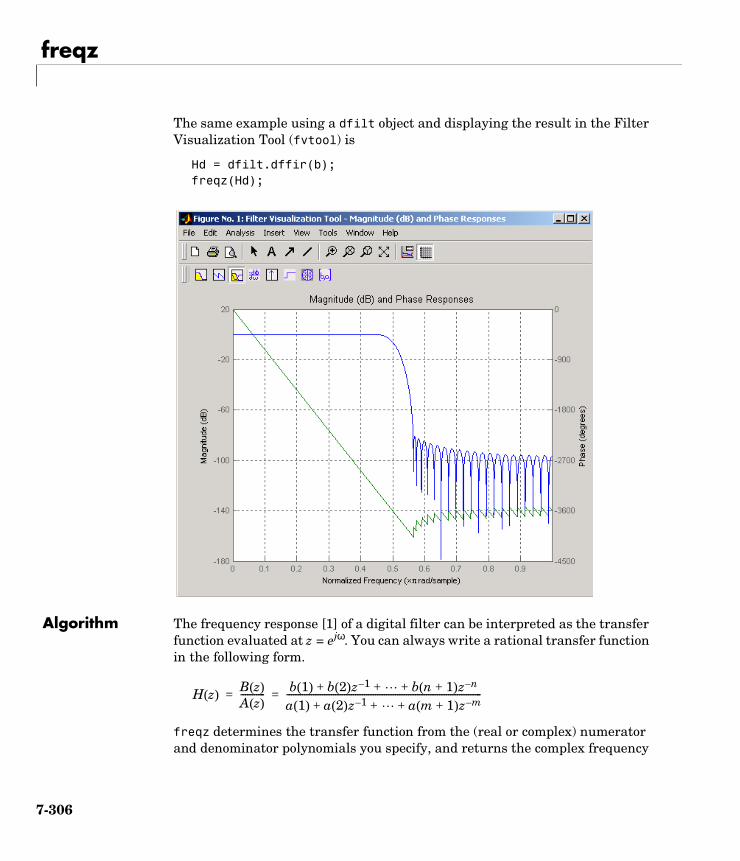
freqz
The same example using a dfilt object and displaying the result in the Filter Visualization Tool (fvtool) is
Hd = dfilt.dffir(b);freqz(Hd);
Algorithm The frequency response [1] of a digital filter can be interpreted as the transfer function evaluated at z = ejω. You can always write a rational transfer function in the following form.
freqz determines the transfer function from the (real or complex) numerator and denominator polynomials you specify, and returns the complex frequency
H z( )B z( )A z( )----------- b 1( ) b 2( )z 1– b n 1+( )z n–+ + +
a 1( ) a 2( )z 1– a m 1+( )z m–+ + +----------------------------------------------------------------------------------------= =
7-306
freqz
response H(ejω) of a digital filter. The frequency response is evaluated at sample points determined by the syntax that you use.
freqz generally uses an FFT algorithm to compute the frequency response whenever you don’t supply a vector of frequencies as an input argument. It computes the frequency response as the ratio of the transformed numerator and denominator coefficients, padded with zeros to the desired length.
When you do supply a vector of frequencies as an input argument, then freqz evaluates the polynomials at each frequency point using Horner’s method of nested polynomial evaluation [1], dividing the numerator response by the denominator response.
See Also abs, angle, fft, filter, freqs, impz, invfreqs, logspace
References [1] Oppenheim, A.V., and R.W. Schafer, Discrete-Time Signal Processing, Prentice-Hall, 1989, pp. 203-205.
7-307
fvtool
7fvtoolPurpose Open the Filter Visualization Tool (FVTool)
Syntax fvtool(b,a)fvtool(b1,a1,b2,a2,...bn,an)fvtool(Hd1,Hd2,...)h = fvtool(...)
Description fvtool(b,a) opens FVTool and computes the magnitude response of the digital filter defined with numerator, b and denominator, a. Using FVTool you can display the phase response, group delay, impulse response, step response, pole-zero plot, and coefficients of the filter. You can export the displayed response to a file with Export on the File menu.
fvtool(b1,a1,b2,a2,...bn,an) opens FVTool and computes the magnitude responses of multiple filters defined with numerators, b1...bn and denominators, a1...an.
fvtool(Hd1,Hd2,...) opens FVTool and computes the magnitude responses of the filters in the dfilt objects Hd1, Hd2, etc. If you have the Filter Design Toolbox installed, you can also use fvtool(H1,H2,...) to analyze quantized filter objects (dfilt with arithmetic set to 'single'), multirate filter (mfilt) objects, and adaptive filter (adaptfilt) objects.
h = fvtool(...) returns a figure handle h. You can use this handle to interact with FVTool from the command line. See “Controlling FVTool from the MATLAB Command Line” below.
7-308
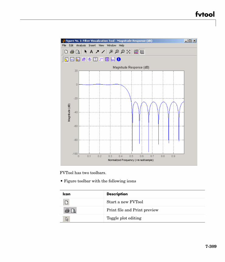
fvtool
FVTool has two toolbars.
• Figure toolbar with the following icons
Icon Description
Start a new FVTool
Print file and Print preview
Toggle plot editing
7-309
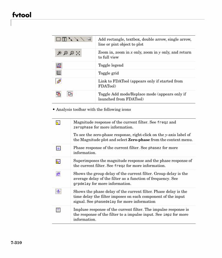
fvtool
• Analysis toolbar with the following icons
Add rectangle, textbox, double arrow, single arrow, line or pint object to plot
Zoom in, zoom in x only, zoom in y only, and return to full view
Toggle legend
Toggle grid
Link to FDATool (appears only if started from FDATool)
Toggle Add mode/Replace mode (appears only if launched from FDATool)
Magnitude response of the current filter. See freqz and zerophase for more information.
To see the zero-phase response, right-click on the y-axis label of the Magnitude plot and select Zero-phase from the context menu.
Phase response of the current filter. See phasez for more information.
Superimposes the magnitude response and the phase response of the current filter. See freqz for more information.
Shows the group delay of the current filter. Group delay is the average delay of the filter as a function of frequency. See grpdelay for more information.
Shows the phase delay of the current filter. Phase delay is the time delay the filter imposes on each component of the input signal. See phasedelay for more information
Impluse response of the current filter. The impulse response is the response of the filter to a impulse input. See impz for more information.
7-310
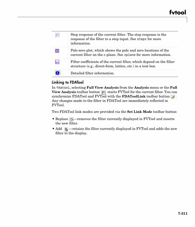
fvtool
Linking to FDAToolIn fdatool, selecting Full View Analysis from the Analysis menu or the Full View Analysis toolbar button starts FVTool for the current filter. You can synchronize FDATool and FVTool with the FDAToolLink toolbar button . Any changes made to the filter in FDATool are immediately reflected in FVTool.
Two FDATool link modes are provided via the Set Link Mode toolbar button:
• Replace —removes the filter currently displayed in FVTool and inserts the new filter.
• Add —retains the filter currently displayed in FVTool and adds the new filter to the display.
Step response of the current filter. The step response is the response of the filter to a step input. See stepz for more information.
Pole-zero plot, which shows the pole and zero locations of the current filter on the z-plane. See zplane for more information.
Filter coefficients of the current filter, which depend on the filter structure (e.g., direct-form, lattice, etc.) in a text box.
Detailed filter information.
7-311
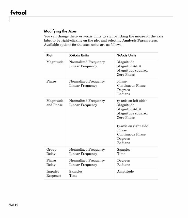
fvtool
Modifying the AxesYou can change the x- or y-axis units by right-clicking the mouse on the axis label or by right-clicking on the plot and selecting Analysis Parameters. Available options for the axes units are as follows.
Plot X-Axis Units Y-Axis Units
Magnitude Normalized FrequencyLinear Frequency
MagnitudeMagnitude(dB)Magnitude squaredZero-Phase
Phase Normalized FrequencyLinear Frequency
PhaseContinuous PhaseDegreesRadians
Magnitude and Phase
Normalized FrequencyLinear Frequency
(y-axis on left side)MagnitudeMagnitude(dB)Magnitude squaredZero-Phase
(y-axis on right side)PhaseContinuous PhaseDegreesRadians
Group Delay
Normalized FrequencyLinear Frequency
SamplesTime
Phase Delay
Normalized FrequencyLinear Frequency
DegreesRadians
Impulse Response
SamplesTime
Amplitude
7-312
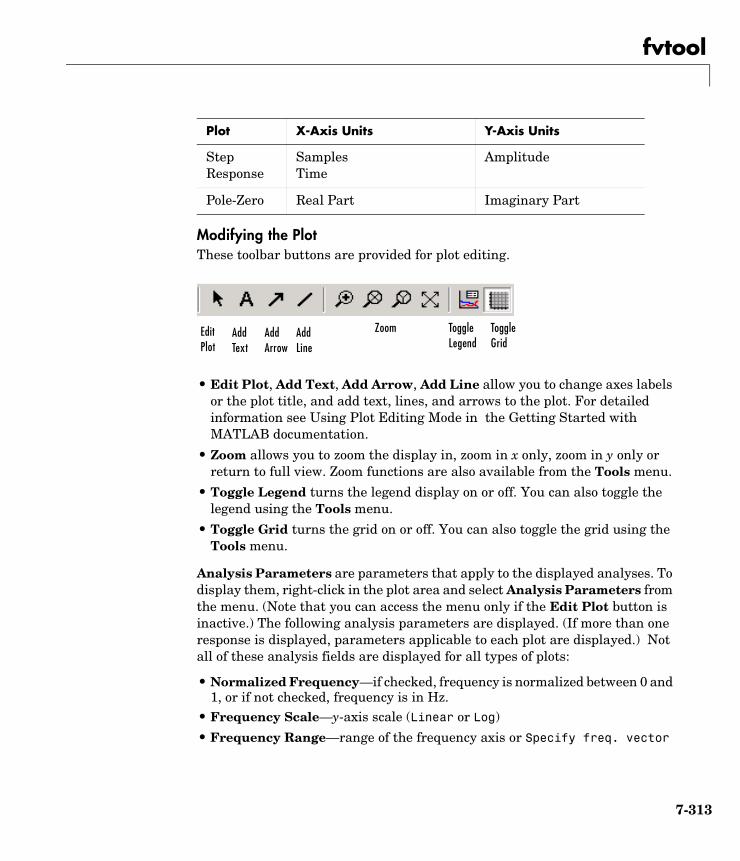
fvtool
Modifying the PlotThese toolbar buttons are provided for plot editing.
• Edit Plot, Add Text, Add Arrow, Add Line allow you to change axes labels or the plot title, and add text, lines, and arrows to the plot. For detailed information see Using Plot Editing Mode in the Getting Started with MATLAB documentation.
• Zoom allows you to zoom the display in, zoom in x only, zoom in y only or return to full view. Zoom functions are also available from the Tools menu.
• Toggle Legend turns the legend display on or off. You can also toggle the legend using the Tools menu.
• Toggle Grid turns the grid on or off. You can also toggle the grid using the Tools menu.
Analysis Parameters are parameters that apply to the displayed analyses. To display them, right-click in the plot area and select Analysis Parameters from the menu. (Note that you can access the menu only if the Edit Plot button is inactive.) The following analysis parameters are displayed. (If more than one response is displayed, parameters applicable to each plot are displayed.) Not all of these analysis fields are displayed for all types of plots:
• Normalized Frequency—if checked, frequency is normalized between 0 and 1, or if not checked, frequency is in Hz.
• Frequency Scale—y-axis scale (Linear or Log)
• Frequency Range—range of the frequency axis or Specify freq. vector
Step Response
SamplesTime
Amplitude
Pole-Zero Real Part Imaginary Part
Plot X-Axis Units Y-Axis Units
Edit Plot
Add Text
Add Arrow
Add Line
Zoom Toggle Legend
Toggle Grid
7-313
fvtool
• Number of Points—number of samples used to compute the response
• Frequency Vector—vector to use for plotting, if Specify freq. vector is selected in Frequency Range.
• Magnitude Display—y-axis units (Magnitude, Magnitude (dB), Magnitude squared, or Zero-Phase)
• Phase Display—type of phase plot (Phase or Continuous Phase)
• Phase Units—y-axis units (Degrees or Radians)
• Group Delay Units—y-axis units (Samples or Time)
• Specify Length—length type of impulse or step response (Default or Specified)
• Length—number of points to use for the impulse or step response
In addition to the above analysis parameters, you can change the plot type for Impulse and Step Response plots by right-clicking and selecting Line with Marker, Stem or Line from the context menu. You can change the x-axis units by right-clicking on the x-axis label and selecting Samples or Time.
To save the displayed parameters as the default values to use when FDATool or FVTool is opened, click Save as default.
To restore the MATLAB-defined default values, click Restore original defaults.
Data Markers display information about a particular point in the plot. See “Using Data Markers” on page 5-16 for more information.
When FVTool is started from FDATool, you can use Design Masks to display filter specifications on a Magnitude plot. See “Analyzing the Filter” on page 5-15 for more information.
Overlaying a ResponseYou can overlay a second response on the plot by selecting Overlay Analysis from the Analysis menu and selecting an available response. A second y-axis is added to the right side of the response plot. The Analysis Parameters dialog box shows parameters for the x-axis and both y-axes.
7-314
fvtool
Controlling FVTool from the MATLAB Command LineAfter you obtain the handle for FVTool, you can control some aspects of FVTool from the command line. In addition to the standard Handle Graphics properties (see Handle Graphics in the MATLAB documentation), FVTool has the following properties:
• 'Filters' — returns a cell array of the filters in FVTool.
• 'Analysis' — displays the specified type of analysis plot. The following table lists the analyses and corresponding analysis strings.
• 'Grid' — controls whether the grid is 'on' or 'off'
• 'Legend' — controls whether the legend is 'on' or 'off'
• 'Fs' — controls the sampling frequency of filters in FVTool. The sampling frequency vector must be of the same length as the number of filters or a
Analysis Type Analysis String
Magnitude plot 'magnitude'
Phase plot 'phase'
Magnitude and Phase plot freq'
Group Delay plot 'grpdelay'
Phase Delay plot phasedelay'
Impulse response plot 'impulse'
Step response plot 'step'
Pole-Zero plot 'polezero'
Filter coefficients 'coefficients'
Filter information 'info'
Magnitude response estimate (available only with Filter Design Toolbox)
'magestimate'
Round-off noise power (available only with Filter Design Toolbox)
'noisepower'
7-315
fvtool
scalar value. If it is a vector, each value is applied to its corresponding filter. If it is a scalar, the same value is applied to all filters.
Note You can change other properties of FVTool from the command line using the set function. Use get(h) to view property tags and current property settings.
You can use the following methods with the FVTool handle.
addfilter(h,filtobj) adds a new filter to FVTool. The new filter, filtobj, must be a dfilt filter object. You can specify the sampling frequency of the new filter with addfilter(h,filtobj,'Fs',10)
setfilter(h,filtobj) replaces the filter in FVTool with the filter specified in filtobj. You can set the sampling frequency as described above.
deletefilter(h, index) deletes the filter at the FVTool cell array index location.
legend(h,str1,str2,...) creates a legend in FVTool by associating str1 with filter 1, str2 with filter 2, etc.
For more information on using FVTool from the command line, see the demo fvtooldemo.
Examples Example 1Display the magnitude response of an elliptic filter, starting FVTool from the command line:
[b,a]=ellip(6,3,50,300/500);fvtool(b,a);
7-316
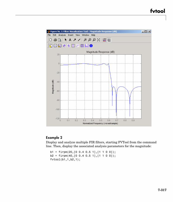
fvtool
Example 2Display and analyze multiple FIR filters, starting FVTool from the command line. Then, display the associated analysis parameters for the magnitude:
b1 = firpm(20,[0 0.4 0.5 1],[1 1 0 0]); b2 = firpm(40,[0 0.4 0.5 1],[1 1 0 0]); fvtool(b1,1,b2,1);
7-317
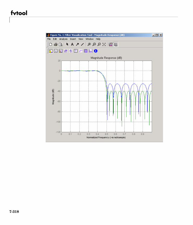
fvtool
7-318
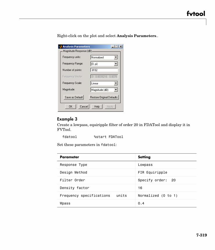
fvtool
Right-click on the plot and select Analysis Parameters..
Example 3Create a lowpass, equiripple filter of order 20 in FDATool and display it in FVTool.
fdatool %start FDATool
Set these parameters in fdatool:
Parameter Setting
Response Type Lowpass
Design Method FIR Equiripple
Filter Order Specify order: 20
Density factor 16
Frequency specifications units Normalized (0 to 1)
Wpass 0.4
7-319
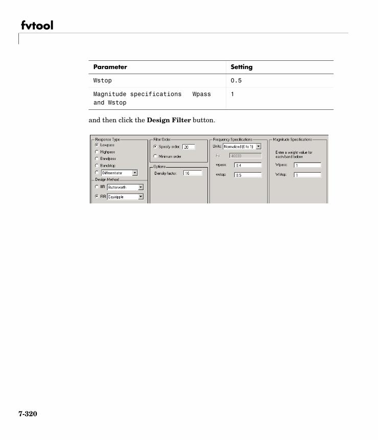
fvtool
and then click the Design Filter button.
Wstop 0.5
Magnitude specifications Wpass and Wstop
1
Parameter Setting
7-320
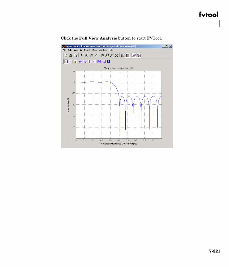
fvtool
Click the Full View Analysis button to start FVTool.
7-321
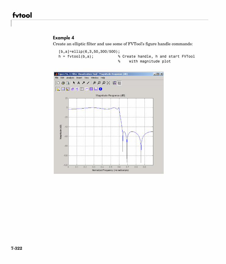
fvtool
Example 4Create an elliptic filter and use some of FVTool’s figure handle commands:
[b,a]=ellip(6,3,50,300/500);h = fvtool(b,a); % Create handle, h and start FVTool
% with magnitude plot
7-322
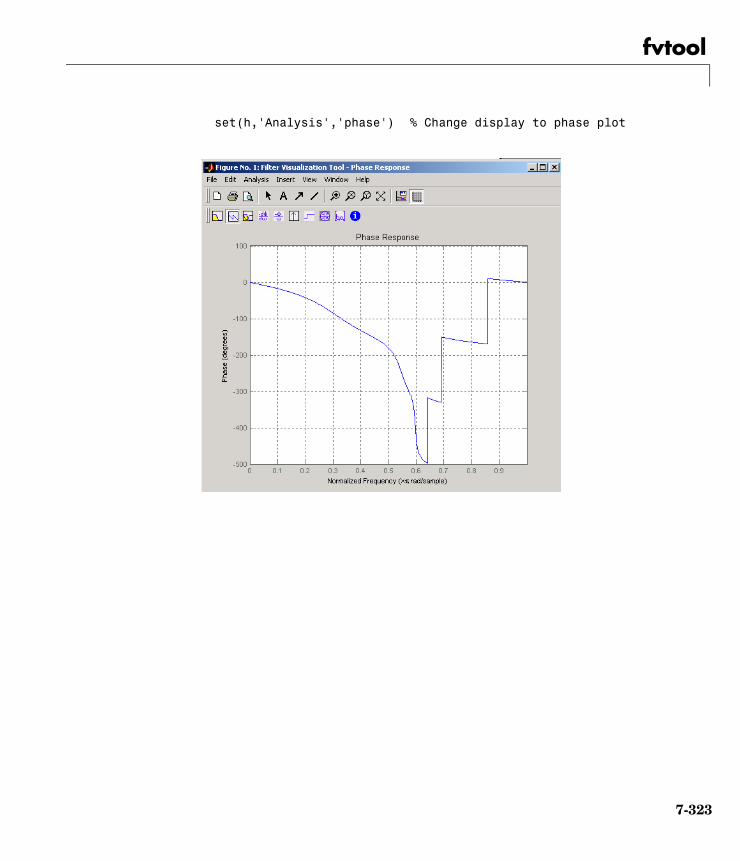
fvtool
set(h,'Analysis','phase') % Change display to phase plot
7-323
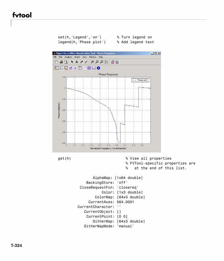
fvtool
set(h,'Legend','on') % Turn legend onlegend(h,'Phase plot') % Add legend text
get(h) % View all properties% FVTool-specific properties are% at the end of this list.
AlphaMap: [1x64 double] BackingStore: 'off' CloseRequestFcn: 'closereq' Color: [1x3 double] ColorMap: [64x3 double] CurrentAxes: 564.0001 CurrentCharacter: '' CurrentObject: [] CurrentPoint: [0 0] DitherMap: [64x3 double] DitherMapMode: 'manual'
7-324
fvtool
DoubleBuffer: 'on' FileName: '' FixedColors: [11x3 double] IntegerHandle: 'on' InvertHardcopy: 'on' KeyPressFcn: '' MenuBar: 'none' MinColormap: 64 Name: [1x42 char] NextPlot: 'new' NumberTitle: 'on' PaperUnits: 'inches' PaperOrientation: 'portrait' PaperPosition: [1x4 double] PaperPositionMode: 'manual' PaperSize: [8.5000 11] PaperType: 'usletter' Pointer: 'arrow' PointerShapeCData: [16x16 double] PointerShapeHotSpot: [1 1] Position: [360 292 560 420] Renderer: 'painters' RendererMode: 'auto' Resize: 'on' ResizeFcn: '' SelectionType: 'normal' ShareColors: 'on' Units: 'pixels' WindowButtonDownFcn: '' WindowButtonMotionFcn: '' WindowButtonUpFcn: '' WindowStyle: 'normal' BeingDeleted: 'off' ButtonDownFcn: '' Children: [15x1 double] Clipping: 'on' CreateFcn: '' DeleteFcn: '' BusyAction: 'queue' HandleVisibility: 'on'
7-325

fvtool
HitTest: 'on' Interruptible: 'on' Parent: 0 Selected: 'off' SelectionHighlight: 'on' Tag: [1x23 char] UIContextMenu: [] UserData: [] Visible: 'on' AnalysisToolbar: 'on' FigureToolbar: 'on' Filters: [1x1 dfilt.df2t] Analysis: 'phase' OverlayedAnalysis: '' Grid: 'on' Legend: 'off' DesignMask: 'off' FrequencyRange: '[0, pi)' NumberofPoints: 8192 FrequencyVector: [1x256 double] FrequencyUnits: 'Normalized' FrequencyScale: 'Linear' PhaseUnits: 'Degrees' PhaseDisplay: 'Phase'
See Also fdatool, sptool
7-326
gauspuls
7gauspulsPurpose Generate a Gaussian-modulated sinusoidal pulse
Syntax yi = gauspuls(t,fc,bw)yi = gauspuls(t,fc,bw,bwr)[yi,yq] = gauspuls(...)[yi,yq,ye] = gauspuls(...)tc = gauspuls('cutoff',fc,bw,bwr,tpe)
Description gauspuls generates Gaussian-modulated sinusoidal pulses.
yi = gauspuls(t,fc,bw) returns a unity-amplitude Gaussian RF pulse at the times indicated in array t, with a center frequency fc in hertz and a fractional bandwidth bw, which must be greater than 0. The default value for fc is 1000 Hz and for bw is 0.5.
yi = gauspuls(t,fc,bw,bwr) returns a unity-amplitude Gaussian RF pulse with a fractional bandwidth of bw as measured at a level of bwr dB with respect to the normalized signal peak. The fractional bandwidth reference level bwr must be less than 0, because it indicates a reference level less than the peak (unity) envelope amplitude. The default value for bwr is -6 dB.
[yi,yq] = gauspuls(...) returns both the in-phase and quadrature pulses.
[yi,yq,ye] = gauspuls(...) returns the RF signal envelope.
tc = gauspuls('cutoff',fc,bw,bwr,tpe) returns the cutoff time tc (greater than or equal to 0) at which the trailing pulse envelope falls below tpe dB with respect to the peak envelope amplitude. The trailing pulse envelope level tpe must be less than 0, because it indicates a reference level less than the peak (unity) envelope amplitude. The default value for tpe is -60 dB.
Remarks Default values are substituted for empty or omitted trailing input arguments.
7-327
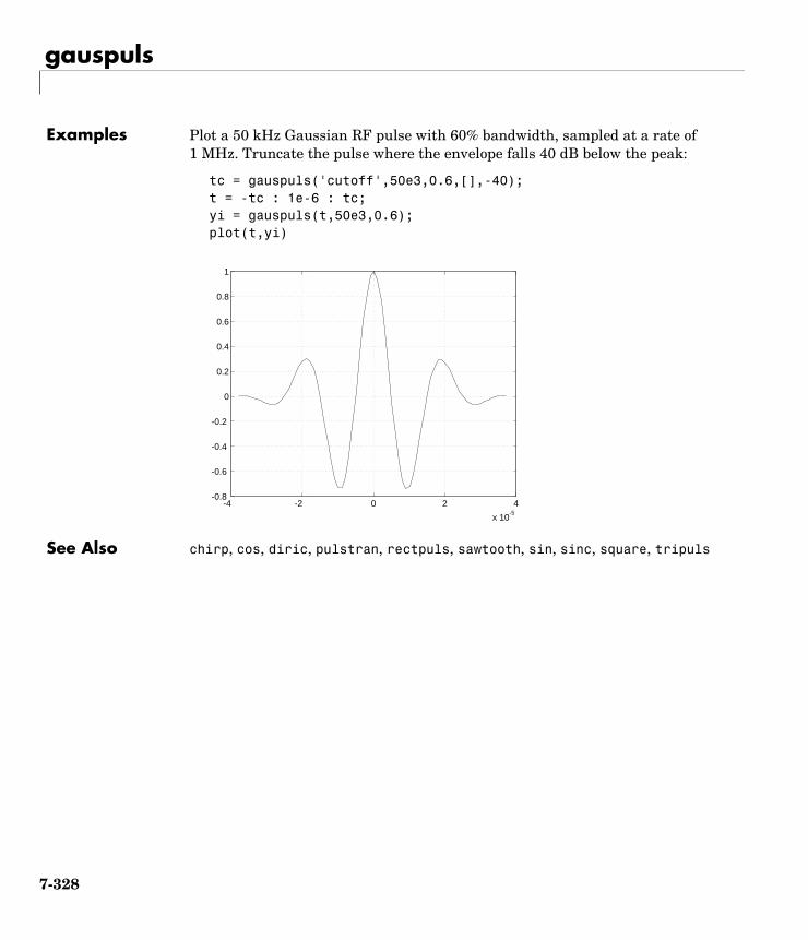
gauspuls
Examples Plot a 50 kHz Gaussian RF pulse with 60% bandwidth, sampled at a rate of 1 MHz. Truncate the pulse where the envelope falls 40 dB below the peak:
tc = gauspuls('cutoff',50e3,0.6,[],-40); t = -tc : 1e-6 : tc; yi = gauspuls(t,50e3,0.6); plot(t,yi)
See Also chirp, cos, diric, pulstran, rectpuls, sawtooth, sin, sinc, square, tripuls
-4 -2 0 2 4
x 10-5
-0.8
-0.6
-0.4
-0.2
0
0.2
0.4
0.6
0.8
1
7-328
gausswin
7gausswinPurpose Compute a Gaussian window
Syntax w = gausswin(n)w = gausswin(n,α)
Description w = gausswin(n) returns an n-point Gaussian window in the column vector w. n is a positive integer. The coefficients of a Gaussian window are computed from the following equation.
where and .
w = gausswin(n,α) returns an n-point Gaussian window where α is the reciprocal of the standard deviation. The width of the window is inversely related to the value of α; a larger value of α produces a more narrow window. If α is omitted, it defaults to 2.5.
Note If the window appears to be clipped, increase the number of points (n) used for gausswin(n) .
Examples Create a 64-point Gaussian window and display the result in WVTool:
N=64;wvtool(gausswin(N))
w k 1+ e
12---– α
k N2----–
N 2⁄--------------
2
=
0 k N≤ ≤ α 2≥
7-329
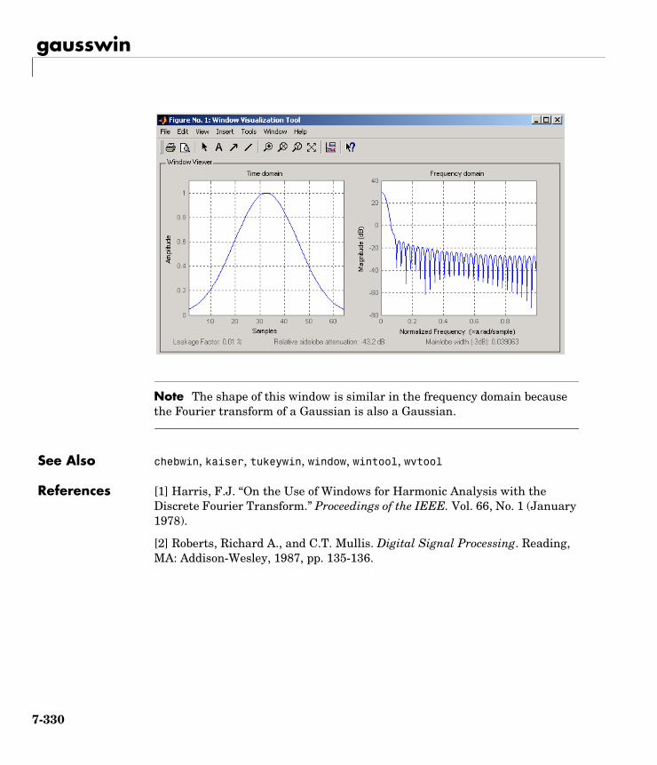
gausswin
Note The shape of this window is similar in the frequency domain because the Fourier transform of a Gaussian is also a Gaussian.
See Also chebwin, kaiser, tukeywin, window, wintool, wvtool
References [1] Harris, F.J. “On the Use of Windows for Harmonic Analysis with the Discrete Fourier Transform.” Proceedings of the IEEE. Vol. 66, No. 1 (January 1978).
[2] Roberts, Richard A., and C.T. Mullis. Digital Signal Processing. Reading, MA: Addison-Wesley, 1987, pp. 135-136.
7-330
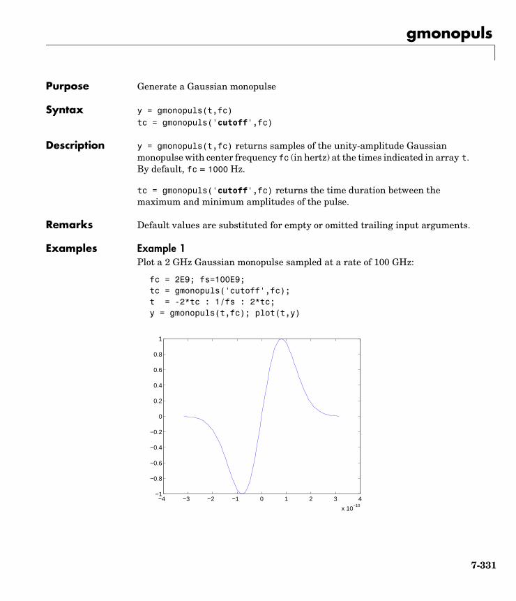
gmonopuls
7gmonopulsPurpose Generate a Gaussian monopulse
Syntax y = gmonopuls(t,fc)tc = gmonopuls('cutoff',fc)
Description y = gmonopuls(t,fc) returns samples of the unity-amplitude Gaussian monopulse with center frequency fc (in hertz) at the times indicated in array t. By default, fc = 1000 Hz.
tc = gmonopuls('cutoff',fc) returns the time duration between the maximum and minimum amplitudes of the pulse.
Remarks Default values are substituted for empty or omitted trailing input arguments.
Examples Example 1Plot a 2 GHz Gaussian monopulse sampled at a rate of 100 GHz:
fc = 2E9; fs=100E9;tc = gmonopuls('cutoff',fc);t = -2*tc : 1/fs : 2*tc;y = gmonopuls(t,fc); plot(t,y)
−4 −3 −2 −1 0 1 2 3 4
x 10−10
−1
−0.8
−0.6
−0.4
−0.2
0
0.2
0.4
0.6
0.8
1
7-331
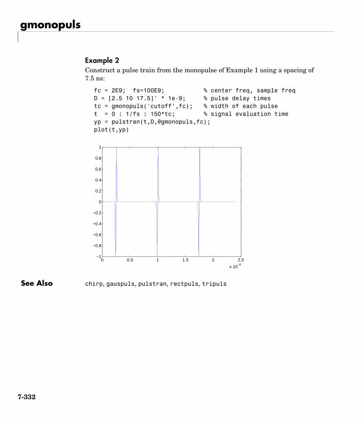
gmonopuls
Example 2Construct a pulse train from the monopulse of Example 1 using a spacing of 7.5 ns:
fc = 2E9; fs=100E9; % center freq, sample freqD = [2.5 10 17.5]' * 1e-9; % pulse delay timestc = gmonopuls('cutoff',fc); % width of each pulset = 0 : 1/fs : 150*tc; % signal evaluation timeyp = pulstran(t,D,@gmonopuls,fc);plot(t,yp)
See Also chirp, gauspuls, pulstran, rectpuls, tripuls
0 0.5 1 1.5 2 2.5
x 10−8
−1
−0.8
−0.6
−0.4
−0.2
0
0.2
0.4
0.6
0.8
1
7-332
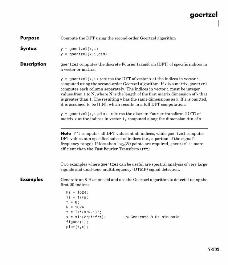
goertzel
7goertzelPurpose Compute the DFT using the second-order Goertzel algorithm
Syntax y = goertzel(x,i)y = goertzel(x,i,dim)
Description goertzel computes the discrete Fourier transform (DFT) of specific indices in a vector or matrix.
y = goertzel(x,i) returns the DFT of vector x at the indices in vector i, computed using the second-order Goertzel algorithm. If x is a matrix, goertzel computes each column separately. The indices in vector i must be integer values from 1 to N, where N is the length of the first matrix dimension of x that is greater than 1. The resulting y has the same dimensions as x. If i is omitted, it is assumed to be [1:N], which results in a full DFT computation.
y = goertzel(x,i,dim) returns the discrete Fourier transform (DFT) of matrix x at the indices in vector i, computed along the dimension dim of x.
Note fft computes all DFT values at all indices, while goertzel computes DFT values at a specified subset of indices (i.e., a portion of the signal’s frequency range). If less than log2(N) points are required, goertzel is more efficient than the Fast Fourier Transform (fft).
Two examples where goertzel can be useful are spectral analysis of very large signals and dual-tone multifrequency (DTMF) signal detection.
Examples Generate an 8-Hz sinusoid and use the Goertzel algorithm to detect it using the first 20 indices:
Fs = 1024;Ts = 1/Fs;f = 8;N = 1024;t = Ts*(0:N-1)';x = sin(2*pi*f*t); % Generate 8 Hz sinusoidfigure(1);plot(t,x);
7-333
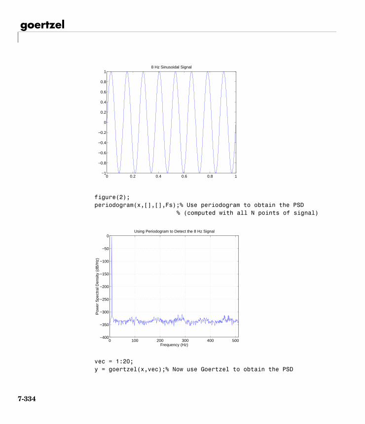
goertzel
figure(2);periodogram(x,[],[],Fs);% Use periodogram to obtain the PSD
% (computed with all N points of signal)
vec = 1:20;y = goertzel(x,vec);% Now use Goertzel to obtain the PSD
0 0.2 0.4 0.6 0.8 1−1
−0.8
−0.6
−0.4
−0.2
0
0.2
0.4
0.6
0.8
18 Hz Sinusoidal Signal
0 100 200 300 400 500−400
−350
−300
−250
−200
−150
−100
−50
0
Frequency (Hz)
Pow
er S
pect
ral D
ensi
ty (
dB/H
z)
Using Periodogram to Detect the 8 Hz Signal
7-334
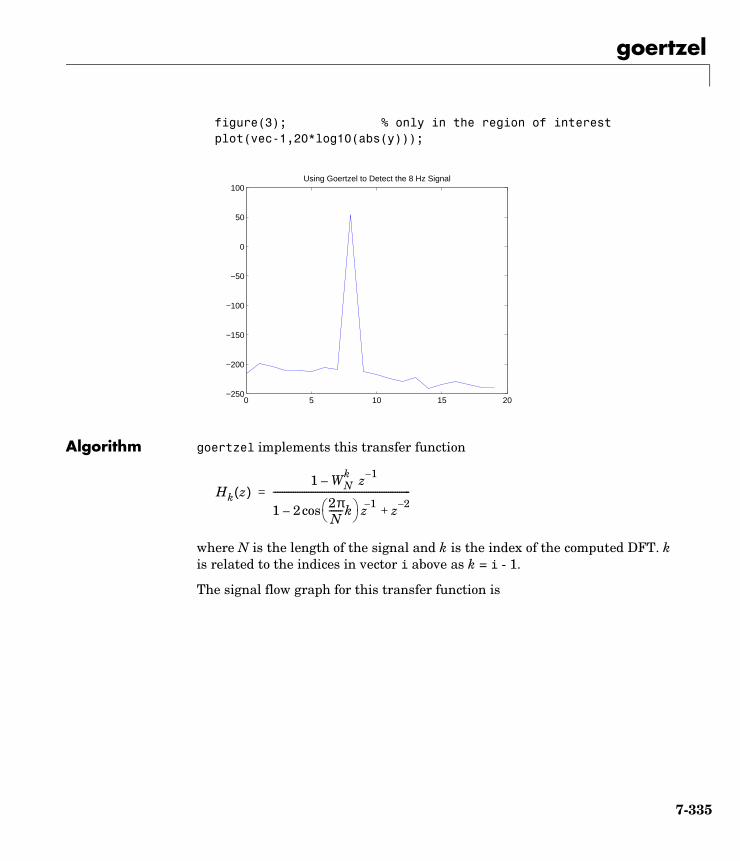
goertzel
figure(3); % only in the region of interestplot(vec-1,20*log10(abs(y)));
Algorithm goertzel implements this transfer function
where N is the length of the signal and k is the index of the computed DFT. k is related to the indices in vector i above as k = i - 1.
The signal flow graph for this transfer function is
0 5 10 15 20−250
−200
−150
−100
−50
0
50
100Using Goertzel to Detect the 8 Hz Signal
Hk z( )1 WN
k z 1––
1 2 2πN------k z 1– z 2–
+cos–
--------------------------------------------------------------=
7-335
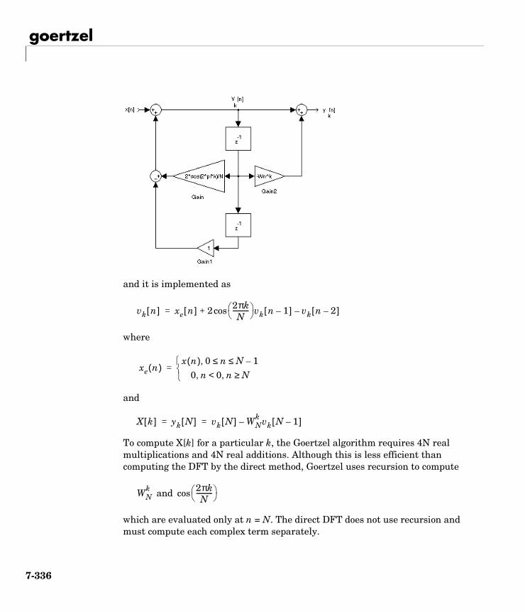
goertzel
and it is implemented as
where
and
To compute X[k] for a particular k, the Goertzel algorithm requires 4N real multiplications and 4N real additions. Although this is less efficient than computing the DFT by the direct method, Goertzel uses recursion to compute
and
which are evaluated only at n = N. The direct DFT does not use recursion and must compute each complex term separately.
vk n[ ] xe n[ ] 2 2πkN
---------- vk n 1–[ ] vk n 2–[ ]–cos+=
xe n( )x n( ) 0, n N 1–≤ ≤
0 n 0 n N≥,<,
=
X k[ ] yk N[ ] vk N[ ] WNk vk N 1–[ ]–= =
WNk 2πk
N---------- cos
7-336

goertzel
See Also fft, fft2
7-337

goertzel
References [1] Burrus, C.S. and T.W. Parks. DFT/FFT and Convolution Algorithms. John Wiley & Sons, 1985, pp. 32-26.
[2] Mitra, Sanjit K. Digital Signal Processing: A Computer-Based Approach. New York, NY: McGraw-Hill, 1998, pp. 520-523.
7-338
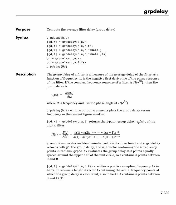
grpdelay
7grpdelayPurpose Compute the average filter delay (group delay)
Syntax grpdelay(b,a)[gd,w] = grpdelay(b,a,n)[gd,f] = grpdelay(b,a,n,fs)[gd,w] = grpdelay(b,a,n,'whole')[gd,f] = grpdelay(b,a,n,'whole',fs)gd = grpdelay(b,a,w)gd = grpdelay(b,a,f,fs)grpdelay(Hd)
Description The group delay of a filter is a measure of the average delay of the filter as a function of frequency. It is the negative first derivative of the phase response of the filter. If the complex frequency response of a filter is , then the group delay is
where ω is frequency and θ is the phase angle of .
grpdelay(b,a) with no output arguments plots the group delay versus frequency in the current figure window.
[gd,w] = grpdelay(b,a,l) returns the i-point group delay, , of the digital filter
given the numerator and denominator coefficients in vectors b and a. grpdelay returns both gd, the group delay, and w, a vector containing the n frequency points in radians. grpdelay evaluates the group delay at n points equally spaced around the upper half of the unit circle, so w contains n points between 0 and π.
[gd,f] = grpdelay(b,a,n,fs) specifies a positive sampling frequency fs in hertz. It returns a length n vector f containing the actual frequency points at which the group delay is calculated, also in hertz. f contains n points between 0 and fs/2.
H ejω( )
τg ω( )dθ ω( )
dω---------------–=
H ejω( )
τg ω( )
H z( )B z( )A z( )----------- b 1( ) b 2( )z 1– b n 1+( )z n–+ + +
a 1( ) a 2( )z 1– a m 1+( )z m–+ + +----------------------------------------------------------------------------------------= =
7-339
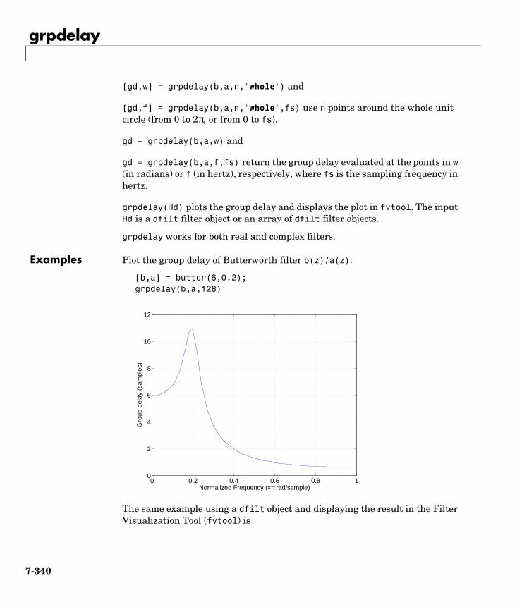
grpdelay
[gd,w] = grpdelay(b,a,n,'whole') and
[gd,f] = grpdelay(b,a,n,'whole',fs) use n points around the whole unit circle (from 0 to 2π, or from 0 to fs).
gd = grpdelay(b,a,w) and
gd = grpdelay(b,a,f,fs) return the group delay evaluated at the points in w (in radians) or f (in hertz), respectively, where fs is the sampling frequency in hertz.
grpdelay(Hd) plots the group delay and displays the plot in fvtool. The input Hd is a dfilt filter object or an array of dfilt filter objects.
grpdelay works for both real and complex filters.
Examples Plot the group delay of Butterworth filter b(z)/a(z):
[b,a] = butter(6,0.2);grpdelay(b,a,128)
The same example using a dfilt object and displaying the result in the Filter Visualization Tool (fvtool) is
0 0.2 0.4 0.6 0.8 10
2
4
6
8
10
12
Normalized Frequency (×π rad/sample)
Gro
up d
elay
(sa
mpl
es)
7-340
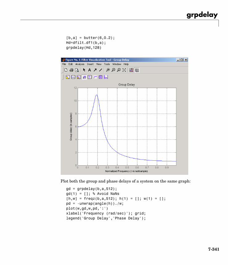
grpdelay
[b,a] = butter(6,0.2);Hd=dfilt.df1(b,a);grpdelay(Hd,128)
Plot both the group and phase delays of a system on the same graph:
gd = grpdelay(b,a,512);gd(1) = []; % Avoid NaNs[h,w] = freqz(b,a,512); h(1) = []; w(1) = [];pd = -unwrap(angle(h))./w;plot(w,gd,w,pd,':')xlabel('Frequency (rad/sec)'); grid;legend('Group Delay','Phase Delay');
7-341
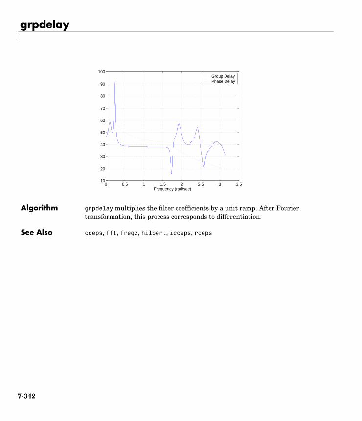
grpdelay
Algorithm grpdelay multiplies the filter coefficients by a unit ramp. After Fourier transformation, this process corresponds to differentiation.
See Also cceps, fft, freqz, hilbert, icceps, rceps
0 0.5 1 1.5 2 2.5 3 3.510
20
30
40
50
60
70
80
90
100
Frequency (rad/sec)
Group DelayPhase Delay
7-342
hamming
7hammingPurpose Compute a Hamming window
Syntax w = hamming(n)w = hamming(n,'sflag')
Description w = hamming(n) returns an n-point symmetric Hamming window in the column vector w. n should be a positive integer. The coefficients of a Hamming window are computed from the following equation.
w = hamming(n,'sflag') returns an n-point Hamming window using the window sampling specified by 'sflag', which can be either 'periodic' or 'symmetric' (the default). When 'periodic' is specified, hamming computes a length n+1 window and returns the first n points.
Note If you specify a one-point window (n=1), the value 1 is returned.
Examples Create a 64-point Hamming window and display the result in WVTool:
N=64;wvtool(hamming(N))
w k 1+[ ] 0.54 0.46 2π kn 1–-------------
cos– k 0= … n 1–, , ,=
7-343
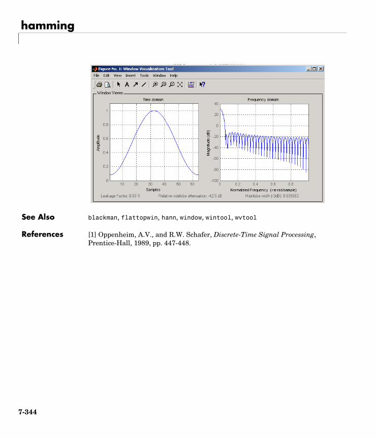
hamming
See Also blackman, flattopwin, hann, window, wintool, wvtool
References [1] Oppenheim, A.V., and R.W. Schafer, Discrete-Time Signal Processing, Prentice-Hall, 1989, pp. 447-448.
7-344
hann
7hannPurpose Compute a Hann (Hanning) window
Syntax w = hann(n)w = hann(n,'sflag')
Description w = hann(n) returns an n-point symmetric Hann window in the column vector w. n must be a positive integer. The coefficients of a Hann window are computed from the following equation.
w = hann(n,'sflag') returns an n-point Hann window using the window sampling specified by 'sflag', which can be either 'periodic' or 'symmetric' (the default). When 'periodic' is specified, hann computes a length n+1 window and returns the first n points.
Note If you specify a one-point window (n=1), the value 1 is returned.
Examples Create a 64-point Hann window and display the result in WVTool:
N=64;wvtool(hann(N))
w k 1+[ ] 0.5 1 2π kn 1–-------------
cos– k 0= … n 1–, , ,=
7-345
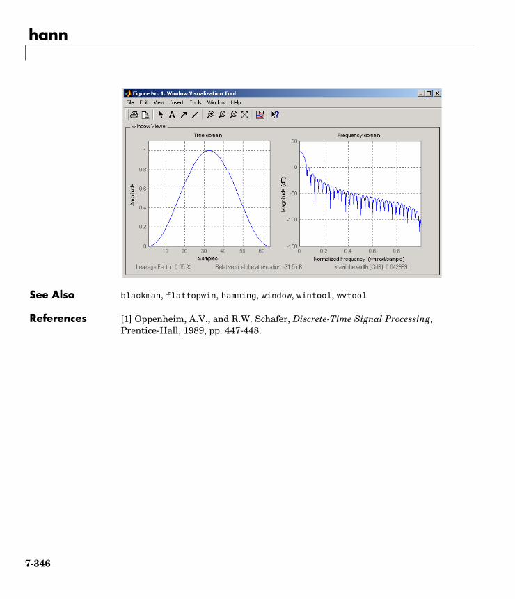
hann
See Also blackman, flattopwin, hamming, window, wintool, wvtool
References [1] Oppenheim, A.V., and R.W. Schafer, Discrete-Time Signal Processing, Prentice-Hall, 1989, pp. 447-448.
7-346
hilbert
7hilbertPurpose Compute the discrete-time analytic signal using the Hilbert transform
Syntax x = hilbert(xr)x = hilbert(xr,n)
Description x = hilbert(xr) returns a complex helical sequence, sometimes called the analytic signal, from a real data sequence. The analytic signal x = xr + i*xi has a real part, xr, which is the original data, and an imaginary part, xi, which contains the Hilbert transform. The imaginary part is a version of the original real sequence with a 90° phase shift. Sines are therefore transformed to cosines and vice versa. The Hilbert transformed series has the same amplitude and frequency content as the original real data and includes phase information that depends on the phase of the original data.
If xr is a matrix, x = hilbert(xr) operates columnwise on the matrix, finding the Hilbert transform of each column.
x = hilbert(xr,n) uses an n point FFT to compute the Hilbert transform. The input data xr is zero-padded or truncated to length n, as appropriate.
The Hilbert transform is useful in calculating instantaneous attributes of a time series, especially the amplitude and frequency. The instantaneous amplitude is the amplitude of the complex Hilbert transform; the instantaneous frequency is the time rate of change of the instantaneous phase angle. For a pure sinusoid, the instantaneous amplitude and frequency are constant. The instantaneous phase, however, is a sawtooth, reflecting the way in which the local phase angle varies linearly over a single cycle. For mixtures of sinusoids, the attributes are short term, or local, averages spanning no more than two or three points.
Reference [1] describes the Kolmogorov method for minimum phase reconstruction, which involves taking the Hilbert transform of the logarithm of the spectral density of a time series. The toolbox function rceps performs this reconstruction.
For a discrete-time analytic signal x, the last half of fft(x) is zero, and the first (DC) and center (Nyquist) elements of fft(x) are purely real.
Examples xr = [1 2 3 4];x = hilbert(xr)
7-347
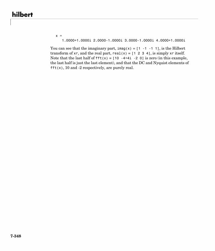
hilbert
x = 1.0000+1.0000i 2.0000-1.0000i 3.0000-1.0000i 4.0000+1.0000i
You can see that the imaginary part, imag(x) = [1 -1 -1 1], is the Hilbert transform of xr, and the real part, real(x) = [1 2 3 4], is simply xr itself. Note that the last half of fft(x) = [10 -4+4i -2 0] is zero (in this example, the last half is just the last element), and that the DC and Nyquist elements of fft(x), 10 and -2 respectively, are purely real.
7-348
hilbert
Algorithm The analytic signal for a sequence x has a one-sided Fourier transform, that is, negative frequencies are 0. To approximate the analytic signal, hilbert calculates the FFT of the input sequence, replaces those FFT coefficients that correspond to negative frequencies with zeros, and calculates the inverse FFT of the result.
In detail, hilbert uses a four-step algorithm:
1 It calculates the FFT of the input sequence, storing the result in a vector x.
2 It creates a vector h whose elements h(i) have the values:
- 1 for i = 1, (n/2)+1
- 2 for i = 2, 3, ... , (n/2)
- 0 for i = (n/2)+2, ... , n
3 It calculates the element-wise product of x and h.
4 It calculates the inverse FFT of the sequence obtained in step 3 and returns the first n elements of the result.
If the input data xr is a matrix, hilbert operates in a similar manner, extending each step above to handle the matrix case.
See Also fft, ifft, rceps
7-349

hilbert
References [1] Claerbout, J.F., Fundamentals of Geophysical Data Processing, McGraw-Hill, 1976, pp. 59-62.
[2] Marple, S.L., “Computing the discrete-time analytic signal via FFT,” IEEE Transactions on Signal Processing, Vol. 47, No. 9 (September 1999), pp. 2600-2603.
[3] Oppenheim, A.V., and R.W. Schafer, Discrete-Time Signal Processing, 2nd ed., Prentice-Hall, 1998.
7-350
icceps
7iccepsPurpose Inverse complex cepstrum
Syntax x = icceps(xhat,nd)
Description x = icceps(xhat,nd) returns the inverse complex cepstrum of the (assumed real) sequence xhat, removing nd samples of delay. If xhat was obtained with cceps(x), then the amount of delay that was added to x was the element of round(unwrap(angle(fft(x)))/pi) corresponding to π radians.
See Also cceps, hilbert, rceps, unwrap
References [1] Oppenheim, A.V., and R.W. Schafer, Discrete-Time Signal Processing, Prentice-Hall, 1989.
7-351
idct
7idctPurpose Inverse discrete cosine transform
Syntax x = idct(y)x = idct(y,n)
Description The inverse discrete cosine transform reconstructs a sequence from its discrete cosine transform (DCT) coefficients. The idct function is the inverse of the dct function.
x = idct(y) returns the inverse discrete cosine transform of y
where
and N = length(x), which is the same as length(y). The series is indexed from n = 1 and k = 1 instead of the usual n = 0 and k = 0 because MATLAB vectors run from 1 to N instead of from 0 to N-1.
x = idct(y,n) appends zeros or truncates the vector y to length n before transforming.
If y is a matrix, idct transforms its columns.
See Also dct, dct2, idct2, ifft
References [1] Jain, A.K., Fundamentals of Digital Image Processing, Prentice-Hall, 1989.
[2] Pennebaker, W.B., and J.L. Mitchell, JPEG Still Image Data Compression Standard, Van Nostrand Reinhold, 1993, Chapter 4.
x n( ) w k( )y k( )π 2n 1–( ) k 1–( )
2N-------------------------------------------cos
k 1=
N
∑ n 1 … N, ,=,=
w k( )
1N
--------- k 1=,
2N---- 2 k N≤ ≤,
=
7-352

ifft
7ifftPurpose One-dimensional inverse fast Fourier transform
ifft is a MATLAB function.
7-353

ifft2
7ifft2Purpose Two-dimensional inverse fast Fourier transform
ifft2 is a MATLAB function.
7-354
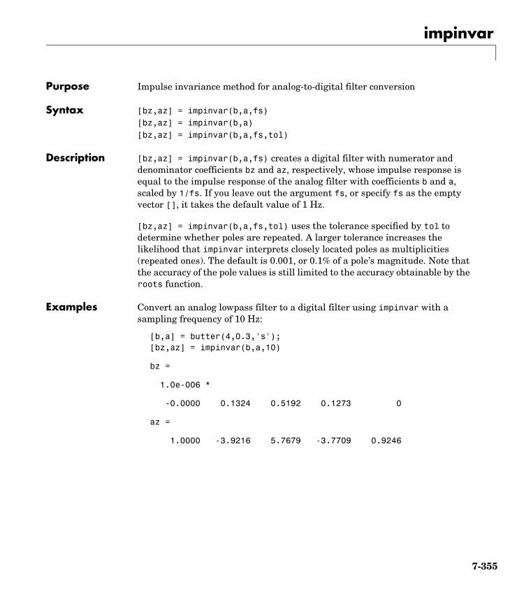
impinvar
7impinvarPurpose Impulse invariance method for analog-to-digital filter conversion
Syntax [bz,az] = impinvar(b,a,fs)[bz,az] = impinvar(b,a)[bz,az] = impinvar(b,a,fs,tol)
Description [bz,az] = impinvar(b,a,fs) creates a digital filter with numerator and denominator coefficients bz and az, respectively, whose impulse response is equal to the impulse response of the analog filter with coefficients b and a, scaled by 1/fs. If you leave out the argument fs, or specify fs as the empty vector [], it takes the default value of 1 Hz.
[bz,az] = impinvar(b,a,fs,tol) uses the tolerance specified by tol to determine whether poles are repeated. A larger tolerance increases the likelihood that impinvar interprets closely located poles as multiplicities (repeated ones). The default is 0.001, or 0.1% of a pole’s magnitude. Note that the accuracy of the pole values is still limited to the accuracy obtainable by the roots function.
Examples Convert an analog lowpass filter to a digital filter using impinvar with a sampling frequency of 10 Hz:
[b,a] = butter(4,0.3,'s');[bz,az] = impinvar(b,a,10)
bz =
1.0e-006 *
-0.0000 0.1324 0.5192 0.1273 0
az =
1.0000 -3.9216 5.7679 -3.7709 0.9246
7-355
impinvar
Algorithm impinvar performs the impulse-invariant method of analog-to-digital transfer function conversion discussed in reference [1]:
1 It finds the partial fraction expansion of the system represented by b and a.
2 It replaces the poles p by the poles exp(p/fs).
3 It finds the transfer function coefficients of the system from the residues from step 1 and the poles from step 2.
See Also bilinear, lp2bp, lp2bs, lp2hp, lp2lp
References [1] Parks, T.W., and C.S. Burrus, Digital Filter Design, John Wiley & Sons, 1987, pp. 206-209.
7-356
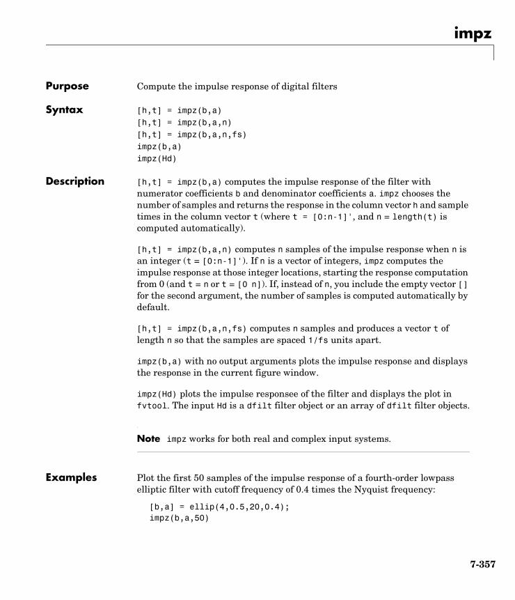
impz
7impzPurpose Compute the impulse response of digital filters
Syntax [h,t] = impz(b,a)[h,t] = impz(b,a,n)[h,t] = impz(b,a,n,fs)impz(b,a)impz(Hd)
Description [h,t] = impz(b,a) computes the impulse response of the filter with numerator coefficients b and denominator coefficients a. impz chooses the number of samples and returns the response in the column vector h and sample times in the column vector t (where t = [0:n-1]', and n = length(t) is computed automatically).
[h,t] = impz(b,a,n) computes n samples of the impulse response when n is an integer (t = [0:n-1]'). If n is a vector of integers, impz computes the impulse response at those integer locations, starting the response computation from 0 (and t = n or t = [0 n]). If, instead of n, you include the empty vector [] for the second argument, the number of samples is computed automatically by default.
[h,t] = impz(b,a,n,fs) computes n samples and produces a vector t of length n so that the samples are spaced 1/fs units apart.
impz(b,a) with no output arguments plots the impulse response and displays the response in the current figure window.
impz(Hd) plots the impulse responsee of the filter and displays the plot in fvtool. The input Hd is a dfilt filter object or an array of dfilt filter objects.
Note impz works for both real and complex input systems.
Examples Plot the first 50 samples of the impulse response of a fourth-order lowpass elliptic filter with cutoff frequency of 0.4 times the Nyquist frequency:
[b,a] = ellip(4,0.5,20,0.4);impz(b,a,50)
7-357
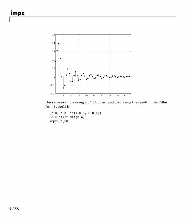
impz
The same example using a dfilt object and displaying the result in the Filter Tool (fvtool) is
[b,a] = ellip(4,0.5,20,0.4);Hd = dfilt.df1(b,a)impz(Hd,50)
0 5 10 15 20 25 30 35 40 45-0.2
-0.1
0
0.1
0.2
0.3
0.4
0.5
7-358
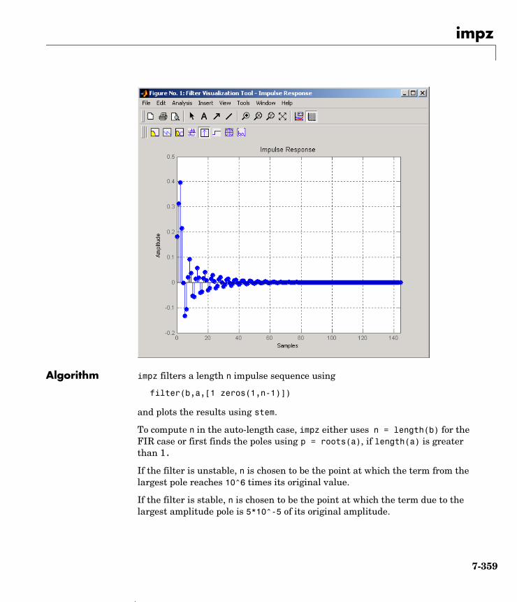
impz
Algorithm impz filters a length n impulse sequence using
filter(b,a,[1 zeros(1,n-1)])
and plots the results using stem.
To compute n in the auto-length case, impz either uses n = length(b) for the FIR case or first finds the poles using p = roots(a), if length(a) is greater than 1.
If the filter is unstable, n is chosen to be the point at which the term from the largest pole reaches 10^6 times its original value.
If the filter is stable, n is chosen to be the point at which the term due to the largest amplitude pole is 5*10^-5 of its original amplitude.
7-359

impz
If the filter is oscillatory (poles on the unit circle only), impz computes five periods of the slowest oscillation.
If the filter has both oscillatory and damped terms, n is chosen to equal five periods of the slowest oscillation or the point at which the term due to the largest (nonunity) amplitude pole is 5*10^-5 of its original amplitude, whichever is greater.
impz also allows for delays in the numerator polynomial. The number of delays is incorporated into the computation for the number of samples.
See Also impulse, stem
7-360
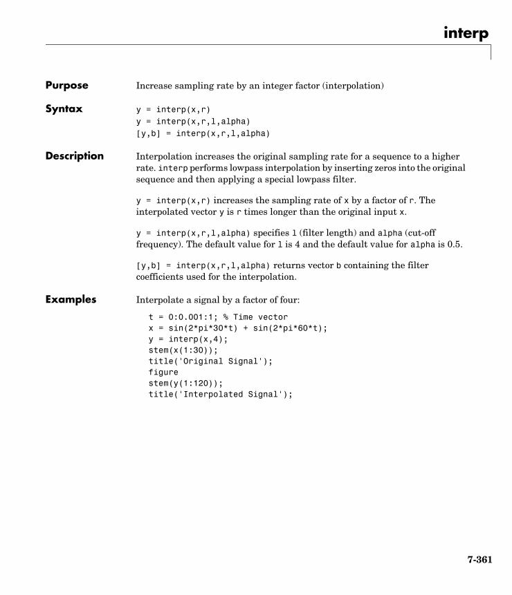
interp
7interpPurpose Increase sampling rate by an integer factor (interpolation)
Syntax y = interp(x,r)y = interp(x,r,l,alpha)[y,b] = interp(x,r,l,alpha)
Description Interpolation increases the original sampling rate for a sequence to a higher rate. interp performs lowpass interpolation by inserting zeros into the original sequence and then applying a special lowpass filter.
y = interp(x,r) increases the sampling rate of x by a factor of r. The interpolated vector y is r times longer than the original input x.
y = interp(x,r,l,alpha) specifies l (filter length) and alpha (cut-off frequency). The default value for l is 4 and the default value for alpha is 0.5.
[y,b] = interp(x,r,l,alpha) returns vector b containing the filter coefficients used for the interpolation.
Examples Interpolate a signal by a factor of four:
t = 0:0.001:1; % Time vectorx = sin(2*pi*30*t) + sin(2*pi*60*t);y = interp(x,4);stem(x(1:30)); title('Original Signal');figurestem(y(1:120)); title('Interpolated Signal');
7-361
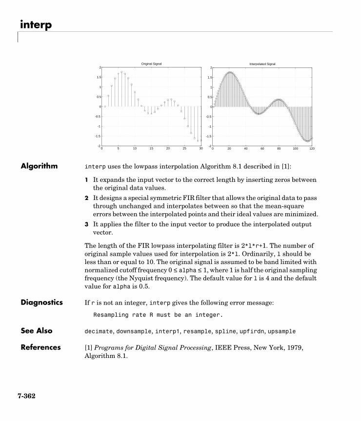
interp
Algorithm interp uses the lowpass interpolation Algorithm 8.1 described in [1]:
1 It expands the input vector to the correct length by inserting zeros between the original data values.
2 It designs a special symmetric FIR filter that allows the original data to pass through unchanged and interpolates between so that the mean-square errors between the interpolated points and their ideal values are minimized.
3 It applies the filter to the input vector to produce the interpolated output vector.
The length of the FIR lowpass interpolating filter is 2*l*r+1. The number of original sample values used for interpolation is 2*l. Ordinarily, l should be less than or equal to 10. The original signal is assumed to be band limited with normalized cutoff frequency 0 ≤ alpha ≤ 1, where 1 is half the original sampling frequency (the Nyquist frequency). The default value for l is 4 and the default value for alpha is 0.5.
Diagnostics If r is not an integer, interp gives the following error message:
Resampling rate R must be an integer.
See Also decimate, downsample, interp1, resample, spline, upfirdn, upsample
References [1] Programs for Digital Signal Processing, IEEE Press, New York, 1979, Algorithm 8.1.
0 20 40 60 80 100 120-2
-1.5
-1
-0.5
0
0.5
1
1.5
2Interpolated Signal
0 5 10 15 20 25 30-2
-1.5
-1
-0.5
0
0.5
1
1.5
2Original Signal
7-362
intfilt
7intfiltPurpose Interpolation FIR filter design
Syntax b = intfilt(r,l,alpha)b = intfilt(r,n,'Lagrange')
Description b = intfilt(r,l,alpha) designs a linear phase FIR filter that performs ideal bandlimited interpolation using the nearest 2*l nonzero samples, when used on a sequence interleaved with r-1 consecutive zeros every r samples. It assumes an original bandlimitedness of alpha times the Nyquist frequency. The returned filter is identical to that used by interp.
b = intfilt(r,n,'Lagrange') or
b = intfilt(r,n,'l') designs an FIR filter that performs nth-order Lagrange polynomial interpolation on a sequence interleaved with r-1 consecutive zeros every r samples. b has length (n + 1)*r for n even, and length (n + 1)*r-1 for n odd.
Both types of filters are basically lowpass and are intended for interpolation and decimation.
Examples Design a digital interpolation filter to upsample a signal by four, using the bandlimited method:
alpha = 0.5; % "Bandlimitedness" factorh1 = intfilt(4,2,alpha); % Bandlimited interpolation
The filter h1 works best when the original signal is bandlimited to alpha times the Nyquist frequency. Create a bandlimited noise signal:
randn('state',0)x = filter(fir1(40,0.5),1,randn(200,1)); % Bandlimit
Now zero pad the signal with three zeros between every sample. The resulting sequence is four times the length of x:
xr = reshape([x zeros(length(x),3)]',4*length(x),1);
Interpolate using the filter command:
y = filter(h1,1,xr);
7-363
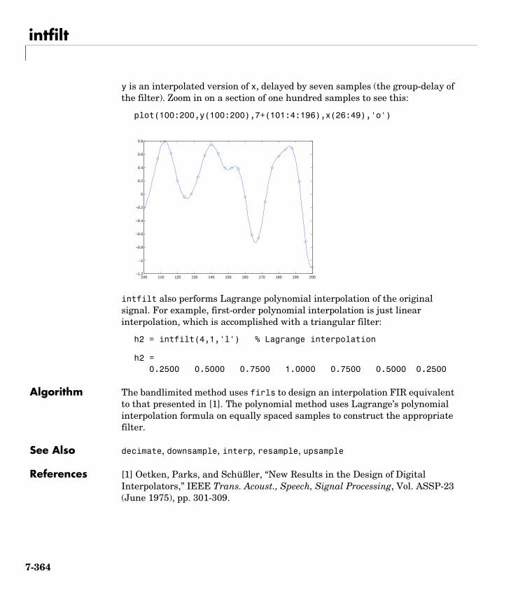
intfilt
y is an interpolated version of x, delayed by seven samples (the group-delay of the filter). Zoom in on a section of one hundred samples to see this:
plot(100:200,y(100:200),7+(101:4:196),x(26:49),'o')
intfilt also performs Lagrange polynomial interpolation of the original signal. For example, first-order polynomial interpolation is just linear interpolation, which is accomplished with a triangular filter:
h2 = intfilt(4,1,'l') % Lagrange interpolation
h2 = 0.2500 0.5000 0.7500 1.0000 0.7500 0.5000 0.2500
Algorithm The bandlimited method uses firls to design an interpolation FIR equivalent to that presented in [1]. The polynomial method uses Lagrange’s polynomial interpolation formula on equally spaced samples to construct the appropriate filter.
See Also decimate, downsample, interp, resample, upsample
References [1] Oetken, Parks, and Schüßler, “New Results in the Design of Digital Interpolators,” IEEE Trans. Acoust., Speech, Signal Processing, Vol. ASSP-23 (June 1975), pp. 301-309.
100 110 120 130 140 150 160 170 180 190 200−1.2
−1
−0.8
−0.6
−0.4
−0.2
0
0.2
0.4
0.6
0.8
7-364

invfreqs
7invfreqsPurpose Identify continuous-time filter parameters from frequency response data
Syntax [b,a] = invfreqs(h,w,n,m)[b,a] = invfreqs(h,w,n,m,wt)[b,a] = invfreqs(h,w,n,m,wt,iter)[b,a] = invfreqs(h,w,n,m,wt,iter,tol)[b,a] = invfreqs(h,w,n,m,wt,iter,tol,'trace')
[b,a] = invfreqs(h,w,'complex',n,m,...)
Description invfreqs is the inverse operation of freqs. It finds a continuous-time transfer function that corresponds to a given complex frequency response. From a laboratory analysis standpoint, invfreqs is useful in converting magnitude and phase data into transfer functions.
[b,a] = invfreqs(h,w,n,m) returns the real numerator and denominator coefficient vectors b and a of the transfer function
whose complex frequency response is given in vector h at the frequency points specified in vector w. Scalars n and m specify the desired orders of the numerator and denominator polynomials.
Frequency is specified in radians between 0 and π, and the length of h must be the same as the length of w. invfreqs uses conj(h) at -w to ensure the proper frequency domain symmetry for a real filter.
[b,a] = invfreqs(h,w,n,m,wt) weights the fit-errors versus frequency, where wt is a vector of weighting factors the same length as w.
[b,a] = invfreqs(h,w,n,m,wt,iter) and
[b,a] = invfreqs(h,w,n,m,wt,iter,tol) provide a superior algorithm that guarantees stability of the resulting linear system and searches for the best fit using a numerical, iterative scheme. The iter parameter tells invfreqs to end the iteration when the solution has converged, or after iter iterations, whichever comes first. invfreqs defines convergence as occurring when the norm of the (modified) gradient vector is less than tol, where tol is an optional parameter that defaults to 0.01. To obtain a weight vector of all ones, use
H s( )B s( )A s( )----------- b 1( )sn b 2( )sn 1– b n 1+( )+ + +
a 1( )sm a 2( )sm 1– a m 1+( )+ + +------------------------------------------------------------------------------------------= =
7-365
invfreqs
invfreqs(h,w,n,m,[],iter,tol)
[b,a] = invfreqs(h,w,n,m,wt,iter,tol,'trace') displays a textual progress report of the iteration.
[b,a] = invfreqs(h,w,'complex',n,m,...) creates a complex filter. In this case no symmetry is enforced, and the frequency is specified in radians between -π and π.
Remarks When building higher order models using high frequencies, it is important to scale the frequencies, dividing by a factor such as half the highest frequency present in w, so as to obtain well conditioned values of a and b. This corresponds to a rescaling of time.
Examples Example 1Convert a simple transfer function to frequency response data and then back to the original filter coefficients:
a = [1 2 3 2 1 4]; b = [1 2 3 2 3];[h,w] = freqs(b,a,64);[bb,aa] = invfreqs(h,w,4,5)
bb =
1.0000 2.0000 3.0000 2.0000 3.0000
aa =
1.0000 2.0000 3.0000 2.0000 1.0000 4.0000
7-366
invfreqs
Notice that bb and aa are equivalent to b and a, respectively. However, aa has poles in the left half-plane and thus the system is unstable. Use invfreqs’s iterative algorithm to find a stable approximation to the system:
[bbb,aaa] = invfreqs(h,w,4,5,[],30)
bbb =
0.6816 2.1015 2.6694 0.9113 -0.1218
aaa =
1.0000 3.4676 7.4060 6.2102 2.5413 0.0001
Example 2Suppose you have two vectors, mag and phase, that contain magnitude and phase data gathered in a laboratory, and a third vector w of frequencies. You can convert the data into a continuous-time transfer function using invfreqs:
[b,a] = invfreqs(mag.*exp(j*phase),w,2,3);
Algorithm By default, invfreqs uses an equation error method to identify the best model from the data. This finds b and a in
by creating a system of linear equations and solving them with the MATLAB \ operator. Here A(w(k)) and B(w(k)) are the Fourier transforms of the polynomials a and b, respectively, at the frequency w(k), and n is the number of frequency points (the length of h and w). This algorithm is based on Levi [1]. Several variants have been suggested in the literature, where the weighting function wt gives less attention to high frequencies.
minb a,
wt k( ) h k( )A w k( )( ) B w k( )( )– 2
k 1=
n
∑
7-367
invfreqs
The superior (“output-error”) algorithm uses the damped Gauss-Newton method for iterative search [2], with the output of the first algorithm as the initial estimate. This solves the direct problem of minimizing the weighted sum of the squared error between the actual and the desired frequency response points.
See Also freqs, freqz, invfreqz, prony
References [1] Levi, E.C., “Complex-Curve Fitting,” IRE Trans. on Automatic Control, Vol. AC-4 (1959), pp. 37-44.
[2] Dennis, J.E., Jr., and R.B. Schnabel. Numerical Methods for Unconstrained Optimization and Nonlinear Equations. Englewood Cliffs, NJ: Prentice-Hall, 1983.
minb a,
wt k( ) h k( )B w k( )( )A w k( )( )--------------------–
2
k 1=
n
∑
7-368
invfreqz
7invfreqzPurpose Identify discrete-time filter parameters from frequency response data
Syntax [b,a] = invfreqz(h,w,n,m)[b,a] = invfreqz(h,w,n,m,wt)[b,a] = invfreqz(h,w,n,m,wt,iter)[b,a] = invfreqz(h,w,n,m,wt,iter,tol)[b,a] = invfreqz(h,w,n,m,wt,iter,tol,'trace')[b,a] = invfreqz(h,w,'complex',n,m,...)
Description invfreqz is the inverse operation of freqz; it finds a discrete-time transfer function that corresponds to a given complex frequency response. From a laboratory analysis standpoint, invfreqz can be used to convert magnitude and phase data into transfer functions.
[b,a] = invfreqz(h,w,n,m) returns the real numerator and denominator coefficients in vectors b and a of the transfer function
whose complex frequency response is given in vector h at the frequency points specified in vector w. Scalars n and m specify the desired orders of the numerator and denominator polynomials.
Frequency is specified in radians between 0 and π, and the length of h must be the same as the length of w. invfreqz uses conj(h) at -w to ensure the proper frequency domain symmetry for a real filter.
[b,a] = invfreqz(h,w,n,m,wt) weights the fit-errors versus frequency, where wt is a vector of weighting factors the same length as w.
[b,a] = invfreqz(h,w,n,m,wt,iter) and
[b,a] = invfreqz(h,w,n,m,wt,iter,tol) provide a superior algorithm that guarantees stability of the resulting linear system and searches for the best fit using a numerical, iterative scheme. The iter parameter tells invfreqz to end the iteration when the solution has converged, or after iter iterations, whichever comes first. invfreqz defines convergence as occurring when the norm of the (modified) gradient vector is less than tol, where tol is an optional parameter that defaults to 0.01. To obtain a weight vector of all ones, use
H z( )B z( )A z( )----------- b 1( ) b 2( )z 1– b n 1+( )z n–+ + +
a 1( ) a 2( )z 1– a m 1+( )z m–+ + +----------------------------------------------------------------------------------------= =
7-369
invfreqz
invfreqz(h,w,n,m,[],iter,tol)
[b,a] = invfreqz(h,w,n,m,wt,iter,tol,'trace') displays a textual progress report of the iteration.
[b,a] = invfreqz(h,w,'complex',n,m,...) creates a complex filter. In this case no symmetry is enforced, and the frequency is specified in radians between -π and π.
Examples Convert a simple transfer function to frequency response data and then back to the original filter coefficients:
a = [1 2 3 2 1 4]; b = [1 2 3 2 3];[h,w] = freqz(b,a,64);[bb,aa] = invfreqz(h,w,4,5)
bb =
1.0000 2.0000 3.0000 2.0000 3.0000
aa =
1.0000 2.0000 3.0000 2.0000 1.0000 4.0000
Notice that bb and aa are equivalent to b and a, respectively. However, aa has poles outside the unit circle and thus the system is unstable. Use invfreqz’s iterative algorithm to find a stable approximation to the system:
[bbb,aaa] = invfreqz(h,w,4,5,[],30)
bbb =
0.2427 0.2788 0.0069 0.0971 0.1980
aaa =
1.0000 -0.8944 0.6954 0.9997 -0.8933 0.6949
Algorithm By default, invfreqz uses an equation error method to identify the best model from the data. This finds b and a in
7-370
invfreqz
by creating a system of linear equations and solving them with the MATLAB \ operator. Here A(ω(k)) and B(ω(k)) are the Fourier transforms of the polynomials a and b, respectively, at the frequency ω(k), and n is the number of frequency points (the length of h and w). This algorithm is a based on Levi [1].
The superior (“output-error”) algorithm uses the damped Gauss-Newton method for iterative search [2], with the output of the first algorithm as the initial estimate. This solves the direct problem of minimizing the weighted sum of the squared error between the actual and the desired frequency response points.
See Also freqs, freqz, invfreqz, prony
References [1] Levi, E.C., “Complex-Curve Fitting,” IRE Trans. on Automatic Control, Vol. AC-4 (1959), pp. 37-44.
[2] Dennis, J.E., Jr., and R.B. Schnabel, Numerical Methods for Unconstrained Optimization and Nonlinear Equations, Prentice-Hall, 1983.
minb a,
wt k( ) h k( )A ω k( )( ) B ω k( )( )– 2
k 1=
n
∑
minb a,
wt k( ) h k( )B ω k( )( )A ω k( )( )-------------------–
2
k 1=
n
∑
7-371
is2rc
7is2rcPurpose Convert inverse sine parameters to reflection coefficients
Syntax k = is2rc(isin)
Description k = is2rc(isin) returns a vector of reflection coefficients k from a vector of inverse sine parameters isin.
Examples isin = [0.2000 0.8727 0.0020 0.0052 -0.0052];k = is2rc(isin)
k = 0.3090 0.9801 0.0031 0.0082 -0.0082
See Also ac2rc, lar2rc, poly2rc, rc2is
References [1] Deller, J.R., J.G. Proakis, and J.H.L. Hansen, “Discrete-Time Processing of Speech Signals,” Prentice-Hall, 1993.
7-372
kaiser
7kaiserPurpose Compute a Kaiser window
Syntax w = kaiser(n,beta)
Description w = kaiser(n,beta) returns an n-point Kaiser (I0 – sinh) window in the column vector w. beta is the Kaiser window β parameter that affects the sidelobe attenuation of the Fourier transform of the window. The default value for beta is 0.5.
To obtain a Kaiser window that designs an FIR filter with sidelobe height -α dB, use the following β.
Increasing beta widens the main lobe and decreases the amplitude of the sidelobes (increases the attenuation).
Examples Create a 200-point Kaiser window with a beta of 2.5 and display the result using WVTool:
w = kaiser(200,2.5);wvtool(w)
β0.1102 α 8.7–( ), α 50>0.5842 α 21–( )0.4 0.07886 α 21–( )+ , 50 α 21≥ ≥0, α 21<
=
7-373
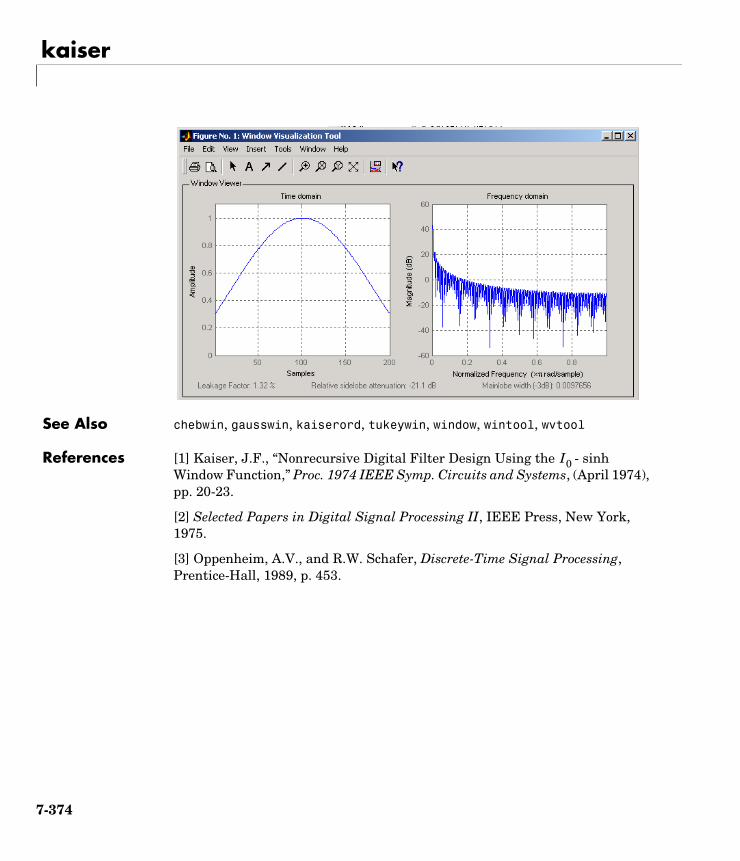
kaiser
See Also chebwin, gausswin, kaiserord, tukeywin, window, wintool, wvtool
References [1] Kaiser, J.F., “Nonrecursive Digital Filter Design Using the - sinh Window Function,” Proc. 1974 IEEE Symp. Circuits and Systems, (April 1974), pp. 20-23.
[2] Selected Papers in Digital Signal Processing II, IEEE Press, New York, 1975.
[3] Oppenheim, A.V., and R.W. Schafer, Discrete-Time Signal Processing, Prentice-Hall, 1989, p. 453.
I0
7-374
kaiserord
7kaiserordPurpose Estimate parameters for an FIR filter design with a Kaiser window
Syntax [n,Wn,beta,ftype] = kaiserord(f,a,dev)[n,Wn,beta,ftype] = kaiserord(f,a,dev,fs)c = kaiserord(f,a,dev,fs,'cell')
Description kaiserord returns a filter order n and beta parameter to specify a Kaiser window for use with the fir1 function. Given a set of specifications in the frequency domain, kaiserord estimates the minimum FIR filter order that will approximately meet the specifications. kaiserord converts the given filter specifications into passband and stopband ripples and converts cutoff frequencies into the form needed for windowed FIR filter design.
[n,Wn,beta,ftype] = kaiserord(f,a,dev) finds the approximate order n, normalized frequency band edges Wn, and weights that meet input specifications f, a, and dev. f is a vector of band edges and a is a vector specifying the desired amplitude on the bands defined by f. The length of f is twice the length of a, minus 2. Together, f and a define a desired piecewise constant response function. dev is a vector the same size as a that specifies the maximum allowable error or deviation between the frequency response of the output filter and its desired amplitude, for each band. The entries in dev specify the passband ripple and the stopband attenuation. You specify each entry in dev as a positive number, representing absolute filter gain (not in decibels).
Note If, in the vector dev, you specify unequal deviations across bands, the minimum specified deviation is used, since the Kaiser window method is constrained to produce filters with minimum deviation in all of the bands.
fir1 can use the resulting order n, frequency vector Wn, multiband magnitude type ftype, and the Kaiser window parameter beta. The ftype string is intended for use with fir1; it is equal to 'high' for a highpass filter and 'stop' for a bandstop filter. For multiband filters, it can be equal to 'dc-0' when the first band is a stopband (starting at f = 0) or 'dc-1' when the first band is a passband.
7-375
kaiserord
To design an FIR filter b that approximately meets the specifications given by kaiser parameters f, a, and dev, use the following command.
b = fir1(n,Wn,kaiser(n+1,beta),ftype,'noscale')
[n,Wn,beta,ftype] = kaiserord(f,a,dev,fs) uses a sampling frequency fs in Hz. If you don’t specify the argument fs, or if you specify it as the empty vector [], it defaults to 2 Hz, and the Nyquist frequency is 1 Hz. You can use this syntax to specify band edges scaled to a particular application’s sampling frequency. The frequency band edges in f must be from 0 to fs/2.
c = kaiserord(f,a,dev,fs,'cell') is a cell-array whose elements are the parameters to fir1.
Note In some cases, kaiserord underestimates or overestimates the order n. If the filter does not meet the specifications, try a higher order such as n+1, n+2, and so on, or a try lower order.
Results are inaccurate if the cutoff frequencies are near 0 or the Nyquist frequency, or if dev is large (greater than 10%).
Remarks Be careful to distinguish between the meanings of filter length and filter order. The filter length is the number of impulse response samples in the FIR filter. Generally, the impulse response is indexed from n = 0 to n = L-1, where L is the filter length. The filter order is the highest power in a z-transform representation of the filter. For an FIR transfer function, this representation is a polynomial in z, where the highest power is zL-1 and the lowest power is z0. The filter order is one less than the length (L-1) and is also equal to the number of zeros of the z polynomial.
Examples Example 1Design a lowpass filter with passband defined from 0 to 1 kHz and stopband defined from 1500 Hz to 4 kHz. Specify a passband ripple of 5% and a stopband attenuation of 40 dB:
fsamp = 8000;
7-376
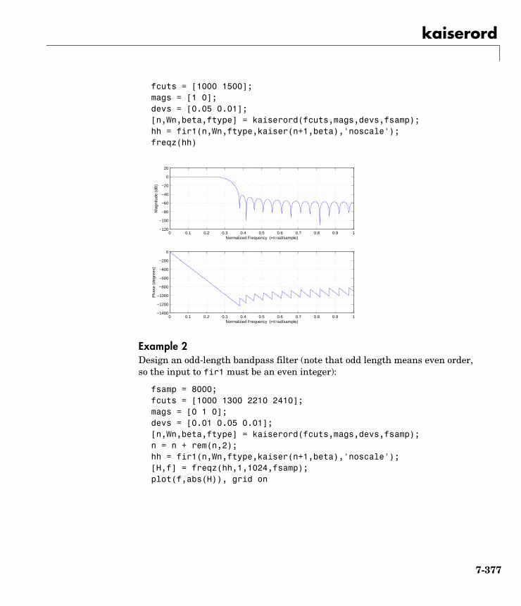
kaiserord
fcuts = [1000 1500];mags = [1 0];devs = [0.05 0.01];[n,Wn,beta,ftype] = kaiserord(fcuts,mags,devs,fsamp);hh = fir1(n,Wn,ftype,kaiser(n+1,beta),'noscale');freqz(hh)
Example 2Design an odd-length bandpass filter (note that odd length means even order, so the input to fir1 must be an even integer):
fsamp = 8000;fcuts = [1000 1300 2210 2410];mags = [0 1 0];devs = [0.01 0.05 0.01];[n,Wn,beta,ftype] = kaiserord(fcuts,mags,devs,fsamp);n = n + rem(n,2);hh = fir1(n,Wn,ftype,kaiser(n+1,beta),'noscale');[H,f] = freqz(hh,1,1024,fsamp);plot(f,abs(H)), grid on
0 0.1 0.2 0.3 0.4 0.5 0.6 0.7 0.8 0.9 1−1400
−1200
−1000
−800
−600
−400
−200
0
Normalized Frequency (×π rad/sample)
Pha
se (
degr
ees)
0 0.1 0.2 0.3 0.4 0.5 0.6 0.7 0.8 0.9 1−120
−100
−80
−60
−40
−20
0
20
Normalized Frequency (×π rad/sample)
Mag
nitu
de (
dB)
7-377
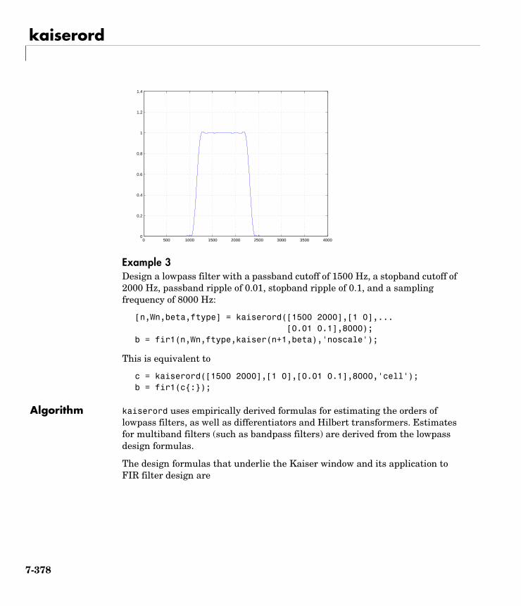
kaiserord
Example 3Design a lowpass filter with a passband cutoff of 1500 Hz, a stopband cutoff of 2000 Hz, passband ripple of 0.01, stopband ripple of 0.1, and a sampling frequency of 8000 Hz:
[n,Wn,beta,ftype] = kaiserord([1500 2000],[1 0],...[0.01 0.1],8000);
b = fir1(n,Wn,ftype,kaiser(n+1,beta),'noscale');
This is equivalent to
c = kaiserord([1500 2000],[1 0],[0.01 0.1],8000,'cell');b = fir1(c:);
Algorithm kaiserord uses empirically derived formulas for estimating the orders of lowpass filters, as well as differentiators and Hilbert transformers. Estimates for multiband filters (such as bandpass filters) are derived from the lowpass design formulas.
The design formulas that underlie the Kaiser window and its application to FIR filter design are
0 500 1000 1500 2000 2500 3000 3500 40000
0.2
0.4
0.6
0.8
1
1.2
1.4
7-378
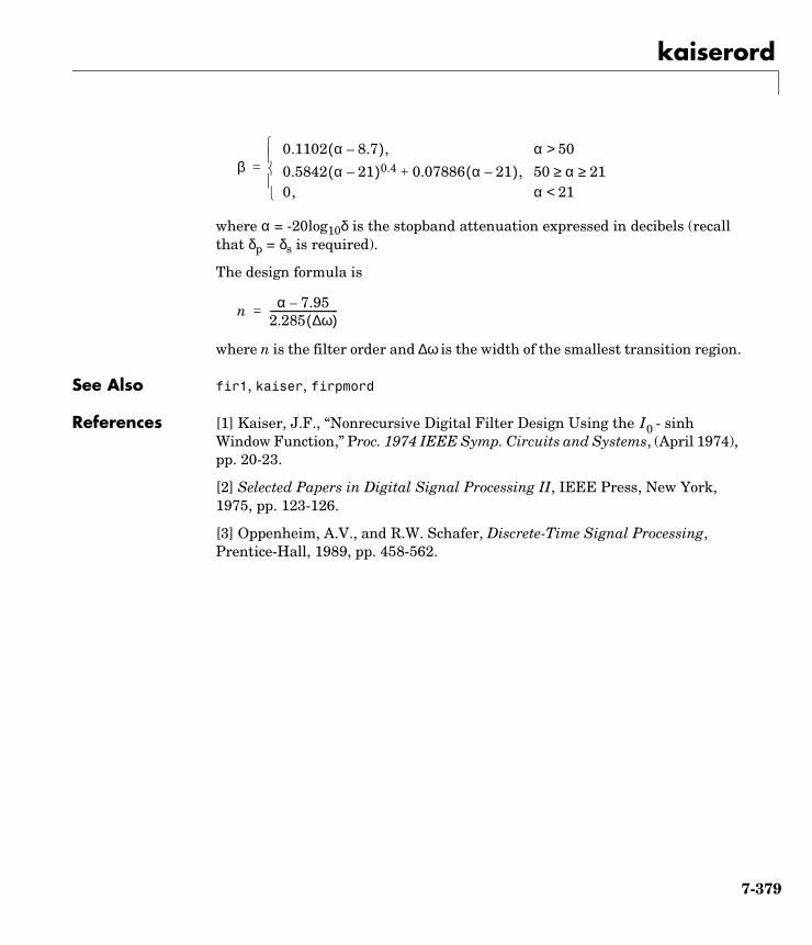
kaiserord
where α = -20log10δ is the stopband attenuation expressed in decibels (recall that δp = δs is required).
The design formula is
where n is the filter order and ∆ω is the width of the smallest transition region.
See Also fir1, kaiser, firpmord
References [1] Kaiser, J.F., “Nonrecursive Digital Filter Design Using the - sinh Window Function,” Proc. 1974 IEEE Symp. Circuits and Systems, (April 1974), pp. 20-23.
[2] Selected Papers in Digital Signal Processing II, IEEE Press, New York, 1975, pp. 123-126.
[3] Oppenheim, A.V., and R.W. Schafer, Discrete-Time Signal Processing, Prentice-Hall, 1989, pp. 458-562.
β0.1102 α 8.7–( ), α 50>0.5842 α 21–( )0.4 0.07886 α 21–( )+ , 50 α 21≥ ≥0, α 21<
=
n α 7.95–2.285 ω∆( )----------------------------=
I0
7-379
lar2rc
7lar2rcPurpose Convert log area ratio parameters to reflection coefficients
Syntax k = lar2rc(g)
Description k = lar2rc(g) returns a vector of reflection coefficients k from a vector of log area ratio parameters g.
Examples g = [0.6389 4.5989 0.0063 0.0163 -0.0163];k = lar2rc(g)
k = 0.3090 0.9801 0.0031 0.0081 -0.0081
See Also ac2rc, is2rc, poly2rc, rc2lar
References [1] Deller, J.R., J.G. Proakis, and J.H.L. Hansen, “Discrete-Time Processing of Speech Signals,” Prentice-Hall, 1993.
7-380
latc2tf
7latc2tfPurpose Convert lattice filter parameters to transfer function form
Syntax [num,den] = latc2tf(k,v)[num,den] = latc2tf(k,'iiroption')num = latc2tf(k,'firoption')num = latc2tf(k)
Description [num,den] = latc2tf(k,v) finds the transfer function numerator num and denominator den from the IIR lattice coefficients k and ladder coefficients v.
[num,den] = latc2tf(k,'iiroption') produces an IIR filter transfer function according to the value of the string 'iiroption':
• 'allpole': Produces an all-pole filter transfer function from the associated all-pole IIR lattice filter coefficients k.
• 'allpass': Produces an allpass filter transfer function from the associated allpass IIR lattice filter coefficients k.
num = latc2tf(k,'firoption') produces an FIR filter according to the value of the string 'firoption':
• 'min': Produces a minimum-phase FIR filter numerator from the associated minimum-phase FIR lattice filter coefficients k.
• 'max': Produces a maximum-phase FIR filter numerator from the associated maximum-phase FIR lattice filter coefficients k.
• 'FIR': Produces a general FIR filter numerator from the lattice filter coefficients k (default, if you leave off the string altogether).
See Also latcfilt, tf2latc
7-381
latcfilt
7latcfiltPurpose Lattice and lattice-ladder filter implementation
Syntax [f,g] = latcfilt(k,x)[f,g] = latcfilt(k,v,x)[f,g] = latcfilt(k,1,x)[f,g,zf] = latcfilt(...,'ic',zi)
Description When filtering data, lattice coefficients can be used to represent
• FIR filters
• All-pole IIR filters
• Allpass IIR filters
• General IIR filters
[f,g] = latcfilt(k,x) filters x with the FIR lattice coefficients in the vector k. f is the forward lattice filter result and g is the backward filter result. If , f corresponds to the minimum-phase output, and g corresponds to the maximum-phase output.
If k and x are vectors, the result is a (signal) vector. Matrix arguments are permitted under the following rules:
• If x is a matrix and k is a vector, each column of x is processed through the lattice filter specified by k.
• If x is a vector and k is a matrix, each column of k is used to filter x, and a signal matrix is returned.
• If x and k are both matrices with the same number of columns, then the ith column of k is used to filter the ith column of x. A signal matrix is returned.
[f,g] = latcfilt(k,v,x) filters x with the IIR lattice coefficients k and ladder coefficients v. k and v must be vectors, while x can be a signal matrix.
[f,g] = latcfilt(k,1,x) filters x with the IIR lattice specified by k, where k and x can be vectors or matrices. f is the all-pole lattice filter result and g is the allpass filter result.
[f,g,zf] = latcfilt(...,'ic',zi) accepts a length-k vector zi specifying the initial condition of the lattice states. Output zf is a length-k vector specifying the final condition of the lattice states.
k 1≤
7-382

latcfilt
See Also filter, latc2tf, tf2latc
7-383
levinson
7levinsonPurpose Compute the Levinson-Durbin recursion
Syntax a = levinson(r,n)[a,e] = levinson(r,n)[a,e,k] = levinson(r,n)
Description The Levinson-Durbin recursion is an algorithm for finding an all-pole IIR filter with a prescribed deterministic autocorrelation sequence. It has applications in filter design, coding, and spectral estimation. The filter that levinson produces is minimum phase.
a = levinson(r,n) finds the coefficients of an nth-order autoregressive linear process which has r as its autocorrelation sequence. r is a real or complex deterministic autocorrelation sequence. If r is a matrix, levinson finds the coefficients for each column of r and returns them in the rows of a. n is the order of denominator polynomial A(z); that is, a = [1 a(2) ... a(n+1)]. The filter coefficients are ordered in descending powers of z.
[a,e] = levinson(r,n) returns the prediction error, e, of order n.
[a,e.k] = levinson(r,n) returns the reflection coefficients k as a column vector of length n.
Note k is computed internally while computing the a coefficients, so returning k simultaneously is more efficient than converting a to k with tf2latc.
Algorithm levinson solves the symmetric Toeplitz system of linear equations
H z( )1
A z( )----------- 1
1 a 2( )z 1– a n 1+( )z n–+ + +-----------------------------------------------------------------------------= =
7-384
levinson
where r = [r(1) ... r(n+1)] is the input autocorrelation vector, and r(i)* denotes the complex conjugate of r(i). The algorithm requires O(n2) flops and is thus much more efficient than the MATLAB \ command for large n. However, the levinson function uses \ for low orders to provide the fastest possible execution.
r 1( ) r 2( )∗ r n( )
∗
r 2( ) r 1( ) r n 1–( )∗
r n( ) r 2( ) r 1( )
a 2( )
a 3( )
a n 1+( )
r 2( )–
r 3( )–
r n 1+( )–
=
7-385

levinson
See Also lpc, prony, rlevinson, schurrc, stmcb
References [1] Ljung, L., System Identification: Theory for the User, Prentice-Hall, 1987, pp. 278-280.
7-386
lp2bp
7lp2bpPurpose Transform lowpass analog filters to bandpass
Syntax [bt,at] = lp2bp(b,a,Wo,Bw)[At,Bt,Ct,Dt] = lp2bp(A,B,C,D,Wo,Bw)
Description lp2bp transforms analog lowpass filter prototypes with a cutoff angular frequency of 1 rad/s into bandpass filters with desired bandwidth and center frequency. The transformation is one step in the digital filter design process for the butter, cheby1, cheby2, and ellip functions.
lp2bp can perform the transformation on two different linear system representations: transfer function form and state-space form. In both cases, the input system must be an analog filter prototype.
Transfer Function Form (Polynomial)
[bt,at] = lp2bp(b,a,Wo,Bw) transforms an analog lowpass filter prototype given by polynomial coefficients into a bandpass filter with center frequency Wo and bandwidth Bw. Row vectors b and a specify the coefficients of the numerator and denominator of the prototype in descending powers of s.
Scalars Wo and Bw specify the center frequency and bandwidth in units of rad/s. For a filter with lower band edge w1 and upper band edge w2, use Wo = sqrt(w1*w2) and Bw = w2-w1.
lp2bp returns the frequency transformed filter in row vectors bt and at.
State-Space Form
[At,Bt,Ct,Dt] = lp2bp(A,B,C,D,Wo,Bw) converts the continuous-time state-space lowpass filter prototype in matrices A, B, C, D shown below
b s( )a s( )---------- b 1( )sn b n( )s b n 1+( )+ + +
a 1( )sm a m( )s a m 1+( )+ + +---------------------------------------------------------------------------------=
x· Ax Bu+=
y Cx Du+=
7-387
lp2bp
into a bandpass filter with center frequency Wo and bandwidth Bw. For a filter with lower band edge w1 and upper band edge w2, use Wo = sqrt(w1*w2) and Bw = w2-w1.
The bandpass filter is returned in matrices At, Bt, Ct, Dt.
Algorithm lp2bp is a highly accurate state-space formulation of the classic analog filter frequency transformation. Consider the state-space system
where u is the input, x is the state vector, and y is the output. The Laplace transform of the first equation (assuming zero initial conditions) is
Now if a bandpass filter is to have center frequency ω0 and bandwidth Bw, the standard s-domain transformation is
where Q = ω0/Bw and p = s/ω0. Substituting this for s in the Laplace transformed state-space equation, and considering the operator p as d/dt results in
or
Now define
which, when substituted, leads to
x· Ax Bu+=
y Cx Du+=
sX s( ) AX s( ) BU s( )+=
s Q p2 1+( ) p⁄=
Qx·· Qx+ A·x Bu·+=
Qx·· A·
– x B– u· Qx–=
Qω· Qx–=
Qx· Ax Qω Bu+ +=
7-388
lp2bp
The last two equations give equations of state. Write them in standard form and multiply the differential equations by ω0 to recover the time/frequency scaling represented by p and find state matrices for the bandpass filter:
Q = Wo/Bw; [ma,m] = size(A);At = Wo*[A/Q eye(ma,m);-eye(ma,m) zeros(ma,m)];Bt = Wo*[B/Q; zeros(ma,n)];Ct = [C zeros(mc,ma)];Dt = d;
If the input to lp2bp is in transfer function form, the function transforms it into state-space form before applying this algorithm.
See Also bilinear, impinvar, lp2bs, lp2hp, lp2lp
7-389
lp2bs
7lp2bsPurpose Transform lowpass analog filters to bandstop
Syntax [bt,at] = lp2bs(b,a,Wo,Bw)[At,Bt,Ct,Dt] = lp2bs(A,B,C,D,Wo,Bw)
Description lp2bs transforms analog lowpass filter prototypes with a cutoff angular frequency of 1 rad/s into bandstop filters with desired bandwidth and center frequency. The transformation is one step in the digital filter design process for the butter, cheby1, cheby2, and ellip functions.
lp2bs can perform the transformation on two different linear system representations: transfer function form and state-space form. In both cases, the input system must be an analog filter prototype.
Transfer Function Form (Polynomial)
[bt,at] = lp2bs(b,a,Wo,Bw) transforms an analog lowpass filter prototype given by polynomial coefficients into a bandstop filter with center frequency Wo and bandwidth Bw. Row vectors b and a specify the coefficients of the numerator and denominator of the prototype in descending powers of s.
Scalars Wo and Bw specify the center frequency and bandwidth in units of radians/second. For a filter with lower band edge w1 and upper band edge w2, use Wo = sqrt(w1*w2) and Bw = w2-w1.
lp2bs returns the frequency transformed filter in row vectors bt and at.
State-Space Form
[At,Bt,Ct,Dt] = lp2bs(A,B,C,D,Wo,Bw) converts the continuous-time state-space lowpass filter prototype in matrices A, B, C, D shown below
b s( )a s( )---------- b 1( )sn b n( )s b n 1+( )+ + +
a 1( )sm a m( )s a m 1+( )+ + +---------------------------------------------------------------------------------=
x· Ax Bu+=
y Cx Du+=
7-390
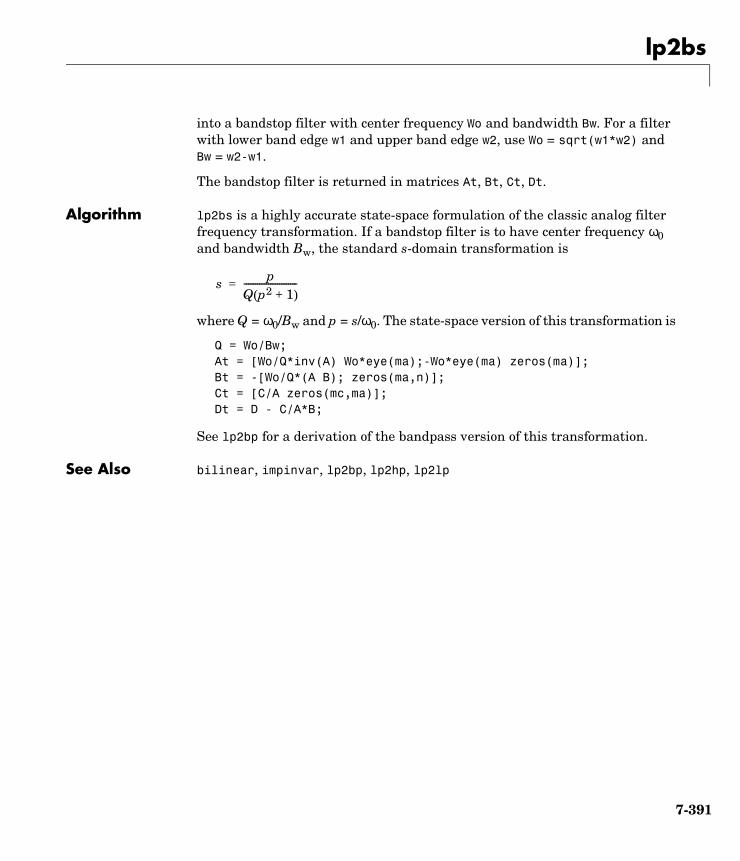
lp2bs
into a bandstop filter with center frequency Wo and bandwidth Bw. For a filter with lower band edge w1 and upper band edge w2, use Wo = sqrt(w1*w2) and Bw = w2-w1.
The bandstop filter is returned in matrices At, Bt, Ct, Dt.
Algorithm lp2bs is a highly accurate state-space formulation of the classic analog filter frequency transformation. If a bandstop filter is to have center frequency ω0 and bandwidth Bw, the standard s-domain transformation is
where Q = ω0/Bw and p = s/ω0. The state-space version of this transformation is
Q = Wo/Bw;At = [Wo/Q*inv(A) Wo*eye(ma);-Wo*eye(ma) zeros(ma)];Bt = -[Wo/Q*(A B); zeros(ma,n)];Ct = [C/A zeros(mc,ma)];Dt = D - C/A*B;
See lp2bp for a derivation of the bandpass version of this transformation.
See Also bilinear, impinvar, lp2bp, lp2hp, lp2lp
s pQ p2 1+( )------------------------=
7-391
lp2hp
7lp2hpPurpose Transform lowpass analog filters to highpass
Syntax [bt,at] = lp2hp(b,a,Wo)[At,Bt,Ct,Dt] = lp2hp(A,B,C,D,Wo)
Description lp2hp transforms analog lowpass filter prototypes with a cutoff angular frequency of 1 rad/s into highpass filters with desired cutoff angular frequency. The transformation is one step in the digital filter design process for the butter, cheby1, cheby2, and ellip functions.
The lp2hp function can perform the transformation on two different linear system representations: transfer function form and state-space form. In both cases, the input system must be an analog filter prototype.
Transfer Function Form (Polynomial)
[bt,at] = lp2hp(b,a,Wo) transforms an analog lowpass filter prototype given by polynomial coefficients into a highpass filter with cutoff angular frequency Wo. Row vectors b and a specify the coefficients of the numerator and denominator of the prototype in descending powers of s.
Scalar Wo specifies the cutoff angular frequency in units of radians/second. The frequency transformed filter is returned in row vectors bt and at.
State-Space Form
[At,Bt,Ct,Dt] = lp2hp(A,B,C,D,Wo) converts the continuous-time state-space lowpass filter prototype in matrices A, B, C, D below
into a highpass filter with cutoff angular frequency Wo. The highpass filter is returned in matrices At, Bt, Ct, Dt.
b s( )a s( )---------- b 1( )sn b n( )s b n 1+( )+ + +
a 1( )sm a m( )s a m 1+( )+ + +---------------------------------------------------------------------------------=
x· Ax Bu+=
y Cx Du+=
7-392
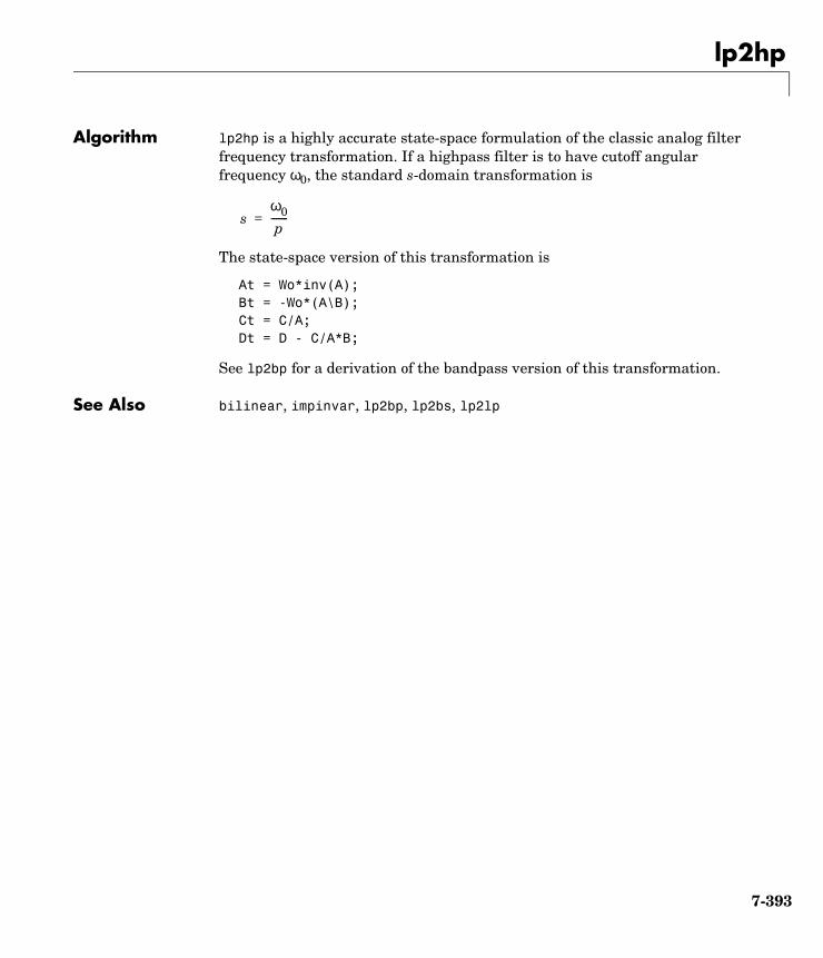
lp2hp
Algorithm lp2hp is a highly accurate state-space formulation of the classic analog filter frequency transformation. If a highpass filter is to have cutoff angular frequency ω0, the standard s-domain transformation is
The state-space version of this transformation is
At = Wo*inv(A);Bt = -Wo*(A\B);Ct = C/A;Dt = D - C/A*B;
See lp2bp for a derivation of the bandpass version of this transformation.
See Also bilinear, impinvar, lp2bp, lp2bs, lp2lp
sω0p
-------=
7-393
lp2lp
7lp2lpPurpose Change the cut-off frequency for a lowpass analog filter
Syntax [bt,at] = lp2lp(b,a,Wo)[At,Bt,Ct,Dt] = lp2lp(A,B,C,D,Wo)
Description lp2lp transforms an analog lowpass filter prototype with a cutoff angular frequency of 1 rad/s into a lowpass filter with any specified cutoff angular frequency. The transformation is one step in the digital filter design process for the butter, cheby1, cheby2, and ellip functions.
The lp2lp function can perform the transformation on two different linear system representations: transfer function form and state-space form. In both cases, the input system must be an analog filter prototype.
Transfer Function Form (Polynomial)
[bt,at] = lp2lp(b,a,Wo) transforms an analog lowpass filter prototype given by polynomial coefficients into a lowpass filter with cutoff angular frequency Wo. Row vectors b and a specify the coefficients of the numerator and denominator of the prototype in descending powers of s.
Scalar Wo specifies the cutoff angular frequency in units of radians/second. lp2lp returns the frequency transformed filter in row vectors bt and at.
State-Space Form
[At,Bt,Ct,Dt] = lp2lp(A,B,C,D,Wo) converts the continuous-time state-space lowpass filter prototype in matrices A, B, C, D below
into a lowpass filter with cutoff angular frequency Wo. lp2lp returns the lowpass filter in matrices At, Bt, Ct, Dt.
b s( )a s( )---------- b 1( )sn b n( )s b n 1+( )+ + +
a 1( )sm a m( )s a m 1+( )+ + +---------------------------------------------------------------------------------=
x· Ax Bu+=
y Cx Du+=
7-394
lp2lp
Algorithm lp2lp is a highly accurate state-space formulation of the classic analog filter frequency transformation. If a lowpass filter is to have cutoff angular frequency ω0, the standard s-domain transformation is
The state-space version of this transformation is
At = Wo*A;Bt = Wo*B;Ct = C;Dt = D;
See lp2bp for a derivation of the bandpass version of this transformation.
See Also bilinear, impinvar, lp2bp, lp2bs, lp2hp
s p ω0⁄=
7-395
lpc
7lpcPurpose Compute linear prediction filter coefficients
Syntax [a,g] = lpc(x,p)
Description lpc determines the coefficients of a forward linear predictor by minimizing the prediction error in the least squares sense. It has applications in filter design and speech coding.
[a,g] = lpc(x,p) finds the coefficients of a pth-order linear predictor (FIR filter) that predicts the current value of the real-valued time series x based on past samples.
p is the order of the prediction filter polynomial, a = [1 a(2) ... a(p+1)]. If p is unspecified, lpc uses as a default p = length(x)-1. If x is a matrix containing a separate signal in each column, lpc returns a model estimate for each column in the rows of matrix a and a row vector of prediction error variances g.
Examples Estimate a data series using a third-order forward predictor, and compare to the original signal.
First, create the signal data as the output of an autoregressive process driven by white noise. Use the last 4096 samples of the AR process output to avoid start-up transients:
randn('state',0);noise = randn(50000,1); % Normalized white Gaussian noisex = filter(1,[1 1/2 1/3 1/4],noise);x = x(45904:50000);
Compute the predictor coefficients, estimated signal, prediction error, and autocorrelation sequence of the prediction error:
a = lpc(x,3);
est_x = filter([0 -a(2:end)],1,x); % Estimated signale = x - est_x; % Prediction error[acs,lags] = xcorr(e,'coeff'); % ACS of prediction error
x n( ) a– 2( )x n 1–( ) a– 3( )x n 2–( ) – a p 1+( )x n p–( )–=
7-396
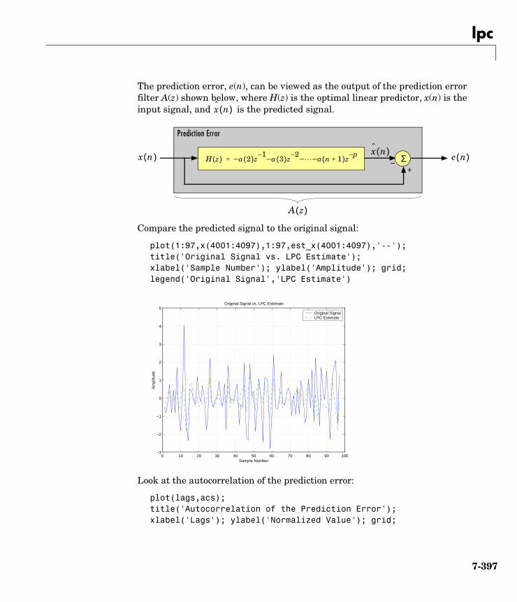
lpc
The prediction error, e(n), can be viewed as the output of the prediction error filter A(z) shown below, where H(z) is the optimal linear predictor, x(n) is the input signal, and is the predicted signal.
Compare the predicted signal to the original signal:
plot(1:97,x(4001:4097),1:97,est_x(4001:4097),'--');title('Original Signal vs. LPC Estimate');xlabel('Sample Number'); ylabel('Amplitude'); grid;legend('Original Signal','LPC Estimate')
Look at the autocorrelation of the prediction error:
plot(lags,acs); title('Autocorrelation of the Prediction Error');xlabel('Lags'); ylabel('Normalized Value'); grid;
x n( )
H z( ) a– 2( )z 1–a– 3( )z 2– – a– n 1+( )z p–
= Σx n( )x n( )
–+
e n( )
Prediction Error
A z( )
0 10 20 30 40 50 60 70 80 90 100−3
−2
−1
0
1
2
3
4
5Original Signal vs. LPC Estimate
Sample Number
Am
plitu
de
Original SignalLPC Estimate
7-397
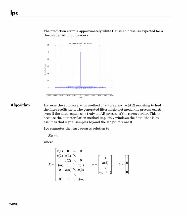
lpc
The prediction error is approximately white Gaussian noise, as expected for a third-order AR input process.
Algorithm lpc uses the autocorrelation method of autoregressive (AR) modeling to find the filter coefficients. The generated filter might not model the process exactly even if the data sequence is truly an AR process of the correct order. This is because the autocorrelation method implicitly windows the data, that is, it assumes that signal samples beyond the length of x are 0.
lpc computes the least squares solution to
where
−5000 −4000 −3000 −2000 −1000 0 1000 2000 3000 4000 5000−0.2
0
0.2
0.4
0.6
0.8
1
1.2Autocorrelation of the Prediction Error
Lags
Nor
mal
ized
Val
ue
Xa b≈
X
x 1( ) 0 0x 2( ) x 1( )
x 2( ) 0x m( ) x 1( )
0 x m( ) x 2( )
0 0 x m( )
= a
1a 2( )
a p 1+( )
= b
10
0
=, ,
7-398
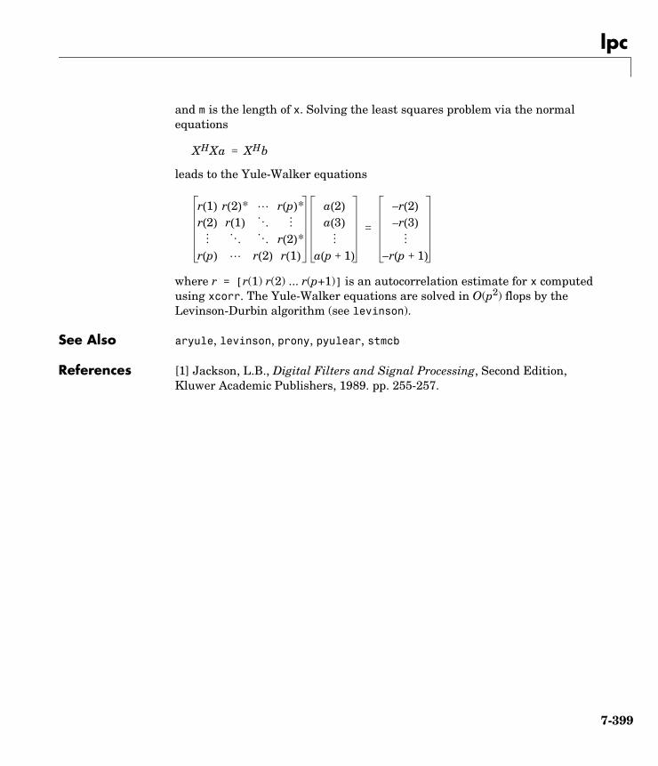
lpc
and m is the length of x. Solving the least squares problem via the normal equations
leads to the Yule-Walker equations
where r = [r(1) r(2) ... r(p+1)] is an autocorrelation estimate for x computed using xcorr. The Yule-Walker equations are solved in O(p2) flops by the Levinson-Durbin algorithm (see levinson).
See Also aryule, levinson, prony, pyulear, stmcb
References [1] Jackson, L.B., Digital Filters and Signal Processing, Second Edition, Kluwer Academic Publishers, 1989. pp. 255-257.
XHXa XHb=
r 1( ) r 2( )* r p( )*r 2( ) r 1( )
r 2( )*r p( ) r 2( ) r 1( )
a 2( )
a 3( )
a p 1+( )
r 2( )–
r 3( )–
r p 1+( )–
=
7-399
lsf2poly
7lsf2polyPurpose Convert line spectral frequencies to prediction filter coefficients
Syntax a = lsf2poly(lsf)
Description a = lsf2poly(lsf) returns a vector a containing the prediction filter coefficients from a vector lsf of line spectral frequencies.
Examples lsf = [0.7842 1.5605 1.8776 1.8984 2.3593];a = lsf2poly(lsf)
a = 1.0000 0.6148 0.9899 0.0001 0.0031 -0.0081
See Also ac2poly, poly2lsf, rc2poly
References [1] Deller, J.R., J.G. Proakis, and J.H.L. Hansen, “Discrete-Time Processing of Speech Signals,” Prentice-Hall, 1993.
[2] Rabiner, L.R., and R.W. Schafer, “Digital Processing of Speech Signals,” Prentice-Hall, 1978.
7-400
maxflat
7maxflatPurpose Generalized digital Butterworth filter design
Syntax [b,a] = maxflat(n,m,Wn)b = maxflat(n,'sym',Wn)[b,a,b1,b2] = maxflat(n,m,Wn)[b,a,b1,b2,sos,g] = maxflat(n,m,Wn)[...] = maxflat(n,m,Wn,'design_flag')
Description [b,a] = maxflat(n,m,Wn) is a lowpass Butterworth filter with numerator and denominator coefficients b and a of orders n and m respectively. Wn is the normalized cutoff frequency at which the magnitude response of the filter is equal to (approx. -3 dB). Wn must be between 0 and 1, where 1 corresponds to the Nyquist frequency.
b = maxflat(n,'sym',Wn) is a symmetric FIR Butterworth filter. n must be even, and Wn is restricted to a subinterval of [0,1]. The function raises an error if Wn is specified outside of this subinterval.
[b,a,b1,b2] = maxflat(n,m,Wn) returns two polynomials b1 and b2 whose product is equal to the numerator polynomial b (that is, b = conv(b1,b2)). b1 contains all the zeros at z = -1, and b2 contains all the other zeros.
[b,a,b1,b2,sos,g] = maxflat(n,m,Wn) returns the second-order sections representation of the filter as the filter matrix sos and the gain g.
[...] = maxflat(n,m,Wn,'design_flag') enables you to monitor the filter design, where 'design_flag' is
• 'trace' for a textual display of the design table used in the design
• 'plots' for plots of the filter’s magnitude, group delay, and zeros and poles
• 'both' for both the textual display and plots
Examples n = 10; m = 2; Wn = 0.2;[b,a] = maxflat(n,m,Wn)fvtool(b,a) % Display the magnitude plot
1 2⁄
7-401
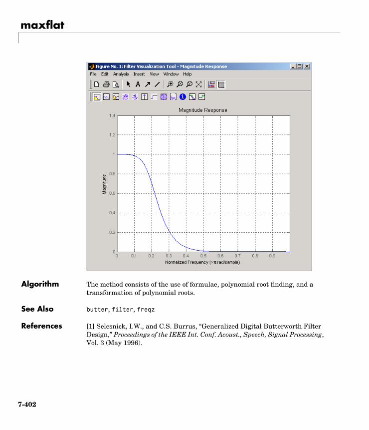
maxflat
Algorithm The method consists of the use of formulae, polynomial root finding, and a transformation of polynomial roots.
See Also butter, filter, freqz
References [1] Selesnick, I.W., and C.S. Burrus, “Generalized Digital Butterworth Filter Design,” Proceedings of the IEEE Int. Conf. Acoust., Speech, Signal Processing, Vol. 3 (May 1996).
7-402
medfilt1
7medfilt1Purpose One-dimensional median filtering
Syntax y = medfilt1(x,n)y = medfilt1(x,n,blksz)
y = medfilt1(x,n,blksz,dim)
Description y = medfilt1(x,n) applies an order n one-dimensional median filter to vector x; the function considers the signal to be 0 beyond the end points. Output y has the same length as x.
For n odd, y(k) is the median of x(k-(n-1)/2:k+(n-1)/2).
For n even, y(k) is the median of x(k-n/2), x(k-(n/2)+1), ..., x(k+(n/2)-1). In this case, medfilt1 sorts the numbers, then takes the average of the n/2 and (n/2)+1 elements.
The default for n is 3.
y = medfilt1(x,n,blksz) uses a for-loop to compute blksz (block size) output samples at a time. Use blksz << length(x) if you are low on memory, since medfilt1 uses a working matrix of size n-by-blksz. By default, blksz = length(x); this provides the fastest execution if you have sufficient memory.
If x is a matrix, medfilt1 median filters its columns using
y(:,i) = medfilt1(x(:,i),n,blksz)
in a loop over the columns of x.
y = medfilt1(x,n,blksz,dim) specifies the dimension, dim, along which the filter operates.
See Also filter, medfilt2, median
References [1] Pratt, W.K., Digital Image Processing, John Wiley & Sons, 1978, pp. 330-333.
7-403
modulate
7modulatePurpose Modulation for communications simulation
Syntax y = modulate(x,fc,fs,'method')y = modulate(x,fc,fs,'method',opt)[y,t] = modulate(x,fc,fs)
Description y = modulate(x,fc,fs,'method') and
y = modulate(x,fc,fs,'method',opt) modulate the real message signal x with a carrier frequency fc and sampling frequency fs, using one of the options listed below for 'method'. Note that some methods accept an option, opt...
Method Description
amdsb-scor
am
Amplitude modulation, double sideband, suppressed carrier. Multiplies x by a sinusoid of frequency fc.
y = x.*cos(2*pi*fc*t)
amdsb-tc Amplitude modulation, double sideband, transmitted carrier. Subtracts scalar opt from x and multiplies the result by a sinusoid of frequency fc.
y = (x-opt).*cos(2*pi*fc*t)
If the opt parameter is not present, modulate uses a default of min(min(x)) so that the message signal (x-opt) is entirely nonnegative and has a minimum value of 0.
amssb Amplitude modulation, single sideband. Multiplies x by a sinusoid of frequency fc and adds the result to the Hilbert transform of x multiplied by a phase shifted sinusoid of frequency fc.
y =x.*cos(2*pi*fc*t)+imag(hilbert(x)).*sin(2*pi*fc*t)
This effectively removes the upper sideband.
7-404
modulate
fm Frequency modulation. Creates a sinusoid with instantaneous frequency that varies with the message signal x.
y = cos(2*pi*fc*t + opt*cumsum(x))
cumsum is a rectangular approximation to the integral of x. modulate uses opt as the constant of frequency modulation. If opt is not present, modulate uses a default of
opt = (fc/fs)*2*pi/(max(max(x)))
so the maximum frequency excursion from fc is fc Hz.
pm Phase modulation. Creates a sinusoid of frequency fc whose phase varies with the message signal x.
y = cos(2*pi*fc*t + opt*x)
modulate uses opt as the constant of phase modulation. If opt is not present, modulate uses a default of
opt = pi/(max(max(x)))
so the maximum phase excursion is π radians.
pwm Pulse-width modulation. Creates a pulse-width modulated signal from the pulse widths in x. The elements of x must be between 0 and 1, specifying the width of each pulse in fractions of a period. The pulses start at the beginning of each period, that is, they are left justified.
modulate(x,fc,fs,'pwm','centered')
yields pulses centered at the beginning of each period. y is length length(x)*fs/fc.
ppm Pulse-position modulation. Creates a pulse-position modulated signal from the pulse positions in x. The elements of x must be between 0 and 1, specifying the left edge of each pulse in fractions of a period. opt is a scalar between 0 and 1 that specifies the length of each pulse in fractions of a period. The default for opt is 0.1. y is length length(x)*fs/fc.
qam Quadrature amplitude modulation. Creates a quadrature amplitude modulated signal from signals x and opt.
y = x.*cos(2*pi*fc*t) + opt.*sin(2*pi*fc*t)
opt must be the same size as x.
7-405

modulate
If you do not specify 'method', then modulate assumes am. Except for the pwm and ptm cases, y is the same size as x.
If x is an array, modulate modulates its columns.
[y,t] = modulate(x,fc,fs) returns the internal time vector t that modulate uses in its computations.
See Also demod, vco, fskdemod, genqamdemod, mskdemod, pamdemod, pmdemod, qamdemod
7-406
mscohere
7mscoherePurpose Estimate magnitude squared coherence function between two signals
Syntax Cxy = mscohere(x,y)Cxy = mscohere(x,y,window)Cxy = mscohere(x,y,window,noverlap)[Cxy,W] = mscohere(x,y,window,noverlap,nfft)[Cxy,F] = mscohere(x,y,window,noverlap,nfft,fs)[...] = mscohere(x,y,...,'whole')mscohere(x,y,...)
Description Cxy = mscohere(x,y) finds the magnitude squared coherence estimate Cxy of the input signals x and y using Welch’s averaged, modified periodogram method. The magnitude squared coherence estimate is a function of frequency with values between 0 and 1 that indicates how well x corresponds to y at each frequency. The coherence is a function of the power spectral density (Pxx and Pyy) of x and y and the cross power spectral density (Pxy) of x and y.
x and y must be the same length. For real x and y, mscohere returns a one-sided coherence estimate and for complex x or y, it returns a two-sided estimate.
Cxy f( )Pxy f( ) 2
Pxx f( )Pyy f( )-------------------------------=
7-407
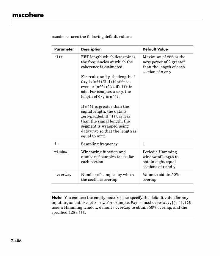
mscohere
mscohere uses the following default values:
Note You can use the empty matrix [] to specify the default value for any input argument except x or y. For example, Pxy = mschoere(x,y,[],[],128 uses a Hamming window, default noverlap to obtain 50% overlap, and the specified 128 nfft.
Parameter Description Default Value
nfft FFT length which determines the frequencies at which the coherence is estimated
For real x and y, the length of Cxy is (nfft/2+1) if nfft is even or (nfft+1)/2 if nfft is odd. For complex x or y, the length of Cxy is nfft.
If nfft is greater than the signal length, the data is zero-padded. If nfft is less than the signal length, the segment is wrapped using datawrap so that the length is equal to nfft.
Maximum of 256 or the next power of 2 greater than the length of each section of x or y
fs Sampling frequency 1
window Windowing function and number of samples to use for each section
Periodic Hamming window of length to obtain eight equal sections of x and y
noverlap Number of samples by which the sections overlap
Value to obtain 50% overlap
7-408
mscohere
Cxy = mscohere(x,y,window) specifies a windowing function, divides x and y into equal overlapping sections of the specified window length, and windows each section using the specified window function. If you supply a scalar for window, Cxy uses a Hamming window of that length. mscohere zero pads the sections if the window length exceeds nfft.
Cxy = mscohere(x,y,window,noverlap) overlaps the sections of x by noverlap samples. noverlap must be an integer smaller than the length of window.
[Pxy,W] = mscohere(x,y,window,noverlap,nfft) uses the specified FFT length nfft to calculate the coherence estimate. It also returns W, which is the vector of normalized frequencies (in rad/sample) at which the coherence is estimated. For real x and y, Cxy length is (nfft/2 +1) if nfft is even and if nfft is odd, the length is (nfft+1)/2. For complex x or y, the length of Cxy is nfft. For real signals, the range of W is [0, pi] when nfft is even and [0, pi) when nfft is odd. For complex signals, the range of W is [0, 2*pi).
[Cxy,F] = mscohere(x,y,window,noverlap,nfft,fs) returns Cxy as a function of frequency and a vector F of frequencies at which the coherence is estimated. fs is the sampling frequency in Hz. For real signals, the range of F is [0, fs/2] when nfft is even and [0, fs/2) when nfft is odd. For complex signals, the range of F is [0, fs).
[...] = mscohere(x,y,...,'whole') returns a coherence estimate with frequencies that range over the whole Nyquist interval. Specifying 'half' uses half the Nyquist interval.
mscohere(...) plots the magnitude squared coherence versus frequency in the current figure window.
Note If you use mscohere on two linearly related signals [1] with a single, non-overlapping window, the output for all frequencies is Cxy = 1.
Examples Compute and plot the coherence estimate between two colored noise sequences x and y:
7-409
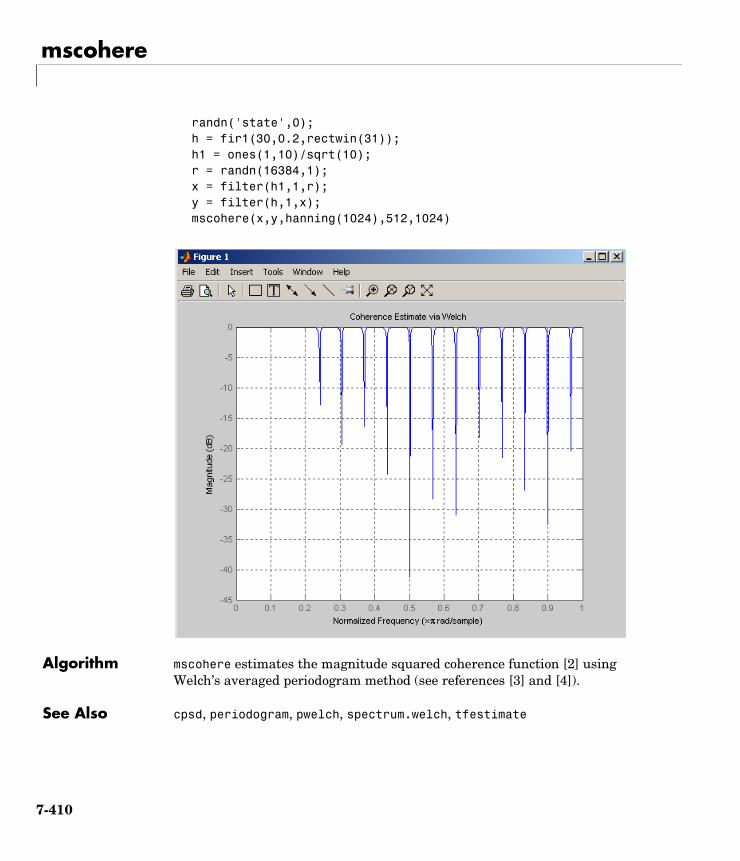
mscohere
randn('state',0);h = fir1(30,0.2,rectwin(31));h1 = ones(1,10)/sqrt(10);r = randn(16384,1);x = filter(h1,1,r);y = filter(h,1,x);mscohere(x,y,hanning(1024),512,1024)
Algorithm mscohere estimates the magnitude squared coherence function [2] using Welch’s averaged periodogram method (see references [3] and [4]).
See Also cpsd, periodogram, pwelch, spectrum.welch, tfestimate
7-410
mscohere
References [1] Stoica, P., and R. Moses. Introduction to Spectral Analysis. Upper Saddle River, NJ: Prentice-Hall, 1997. Pgs. 61-64.
[2] Kay, S.M. Modern Spectral Estimation. Englewood Cliffs, NJ: Prentice-Hall, 1988. Pg. 454.
[3] Rabiner, L.R., and B. Gold. Theory and Application of Digital Signal Processing. Englewood Cliffs, NJ: Prentice-Hall, 1975.
[4] Welch, P.D. “The Use of Fast Fourier Transform for the Estimation of Power Spectra: A Method Based on Time Averaging Over Short, Modified Periodograms.” IEEE Trans. Audio Electroacoust. Vol. AU-15 (June 1967). Pgs. 70-73.
7-411
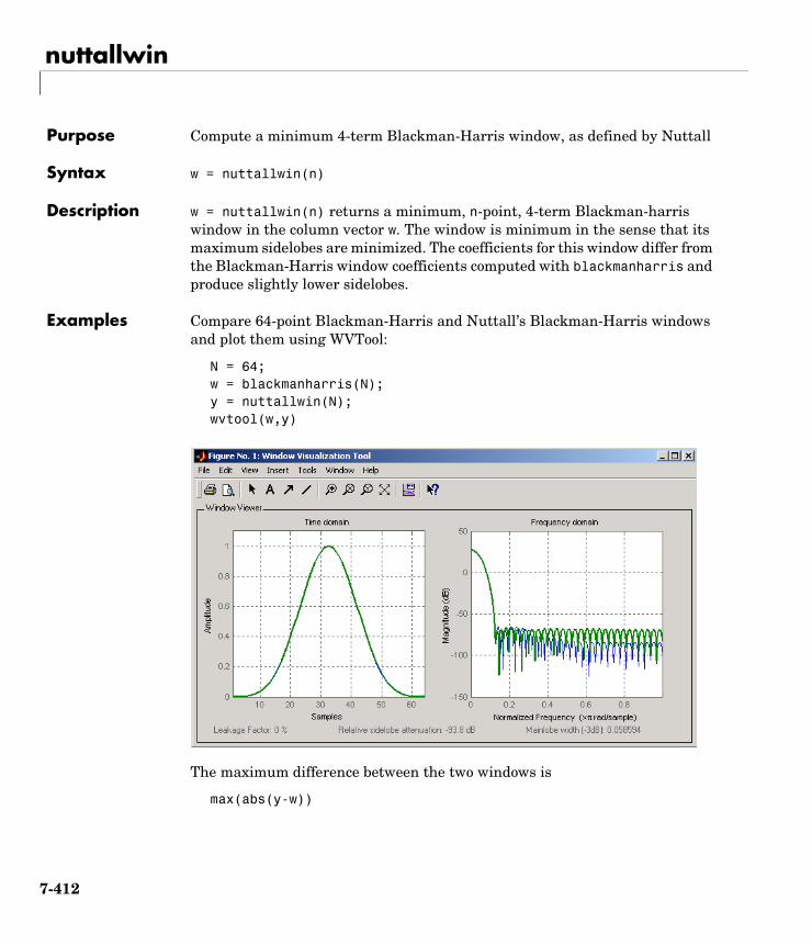
nuttallwin
7nuttallwinPurpose Compute a minimum 4-term Blackman-Harris window, as defined by Nuttall
Syntax w = nuttallwin(n)
Description w = nuttallwin(n) returns a minimum, n-point, 4-term Blackman-harris window in the column vector w. The window is minimum in the sense that its maximum sidelobes are minimized. The coefficients for this window differ from the Blackman-Harris window coefficients computed with blackmanharris and produce slightly lower sidelobes.
Examples Compare 64-point Blackman-Harris and Nuttall’s Blackman-Harris windows and plot them using WVTool:
N = 64;w = blackmanharris(N);y = nuttallwin(N);wvtool(w,y)
The maximum difference between the two windows is
max(abs(y-w))
7-412
nuttallwin
ans =
0.0099
Algorithm The equation for computing the coefficients of a minimum 4-term Blackman-harris window, according to Nuttall, is
where .
The coefficients for this window are
a0 = 0.3635819a1 = 0.4891775a2 = 0.1365995a3 = .0106411
See Also barthannwin, bartlett, blackmanharris, bohmanwin, parzenwin, rectwin, triang, window, wintool, wvtool
References [1] Nuttall, Albert H. “Some Windows with Very Good Sidelobe Behavoir.” IEEE Transactions on Acoustics, Speech, and Signal Processing. Vol. ASSP-29 (February 1981). pp. 84-91.
w k 1+[ ] a0 a1 2π kn 1–-------------
a2 4π kn 1–-------------
cos a3 6π kn 1–-------------
cos–+cos–=
0 k n 1–( )≤ ≤
7-413
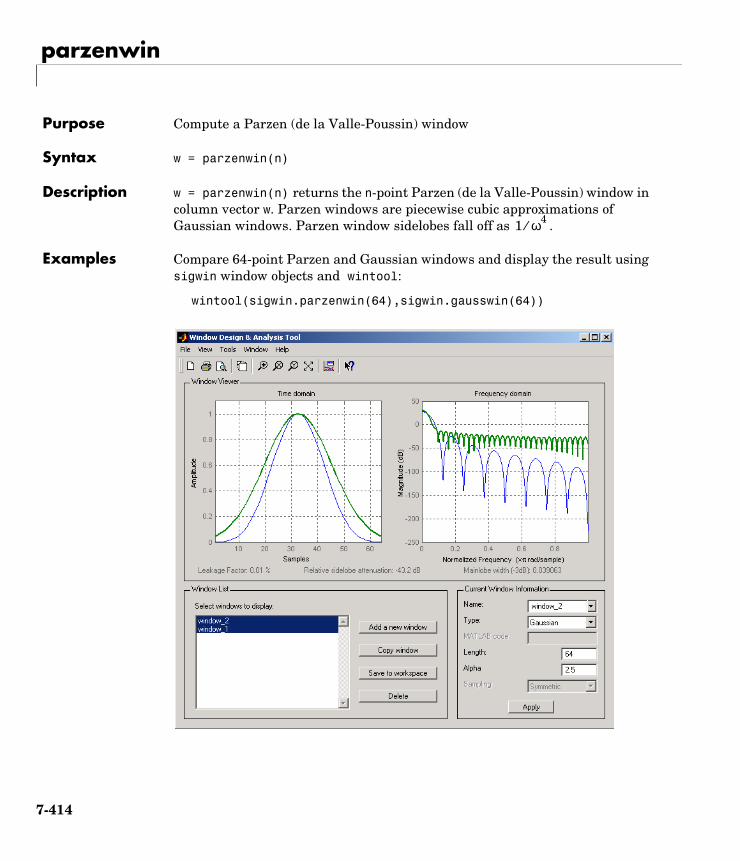
parzenwin
7parzenwinPurpose Compute a Parzen (de la Valle-Poussin) window
Syntax w = parzenwin(n)
Description w = parzenwin(n) returns the n-point Parzen (de la Valle-Poussin) window in column vector w. Parzen windows are piecewise cubic approximations of Gaussian windows. Parzen window sidelobes fall off as .
Examples Compare 64-point Parzen and Gaussian windows and display the result using sigwin window objects and wintool:
wintool(sigwin.parzenwin(64),sigwin.gausswin(64))
1 ω4⁄
7-414
parzenwin
Algorithm The Parzen window is defined as
See Also barthannwin, bartlett, blackmanharris, bohmanwin, nuttallwin, rectwin, triang, window, wintool, wvtool
References Harris, F.J. “On the Use of Windows for Harmonic Analysis with the Discrete Fourier Transform.” Proceedings of the IEEE. Vol. 66, No. 1 (January 1978).
w n( ) 1.0 6 nN 2⁄------------
21.0 n
N 2⁄------------– 0 n N
4----≤ ≤–=
w n( ) 2 1.0 nN 2⁄------------–
3 N4---- n N
2----≤ ≤=
7-415
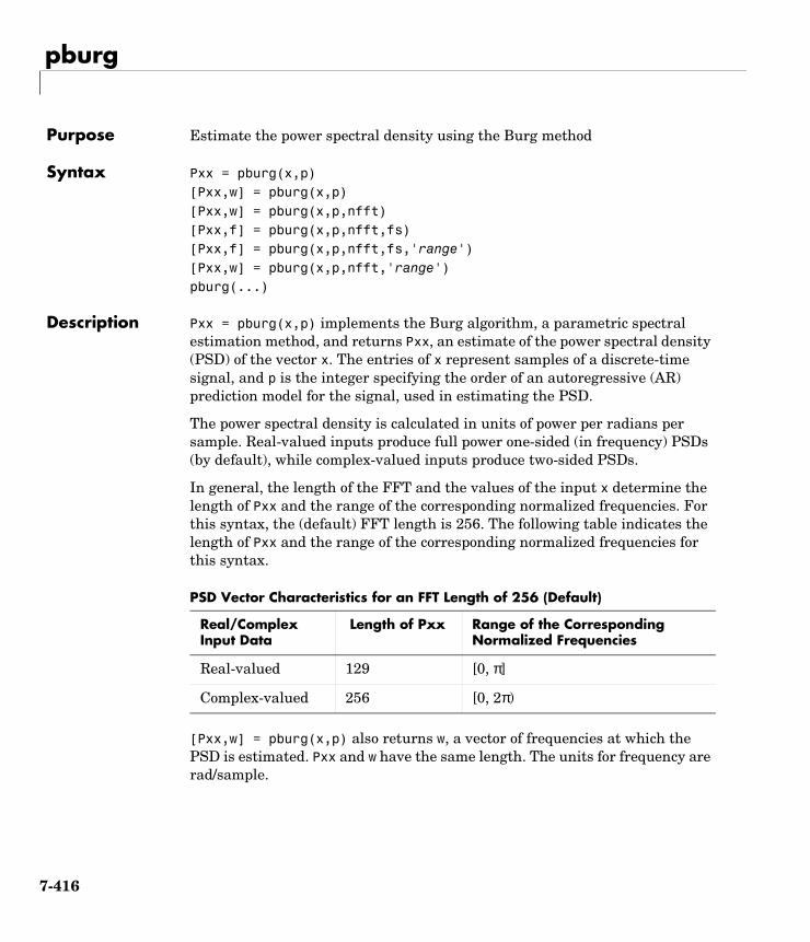
pburg
7pburgPurpose Estimate the power spectral density using the Burg method
Syntax Pxx = pburg(x,p)[Pxx,w] = pburg(x,p)[Pxx,w] = pburg(x,p,nfft)[Pxx,f] = pburg(x,p,nfft,fs)[Pxx,f] = pburg(x,p,nfft,fs,'range')[Pxx,w] = pburg(x,p,nfft,'range')pburg(...)
Description Pxx = pburg(x,p) implements the Burg algorithm, a parametric spectral estimation method, and returns Pxx, an estimate of the power spectral density (PSD) of the vector x. The entries of x represent samples of a discrete-time signal, and p is the integer specifying the order of an autoregressive (AR) prediction model for the signal, used in estimating the PSD.
The power spectral density is calculated in units of power per radians per sample. Real-valued inputs produce full power one-sided (in frequency) PSDs (by default), while complex-valued inputs produce two-sided PSDs.
In general, the length of the FFT and the values of the input x determine the length of Pxx and the range of the corresponding normalized frequencies. For this syntax, the (default) FFT length is 256. The following table indicates the length of Pxx and the range of the corresponding normalized frequencies for this syntax.
[Pxx,w] = pburg(x,p) also returns w, a vector of frequencies at which the PSD is estimated. Pxx and w have the same length. The units for frequency are rad/sample.
PSD Vector Characteristics for an FFT Length of 256 (Default)
Real/Complex Input Data
Length of Pxx Range of the Corresponding Normalized Frequencies
Real-valued 129 [0, π]
Complex-valued 256 [0, 2π)
7-416
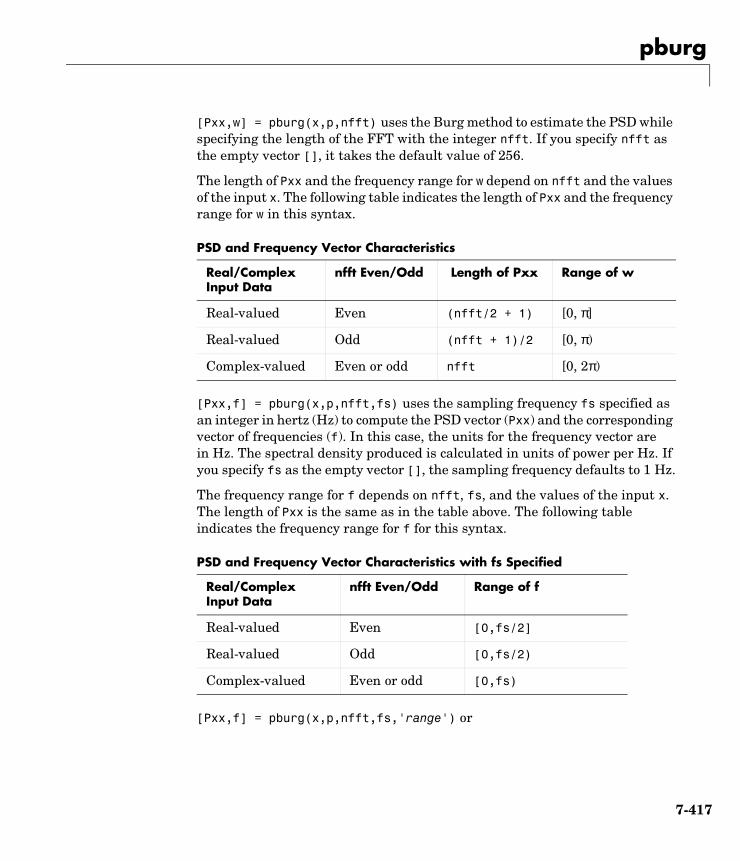
pburg
[Pxx,w] = pburg(x,p,nfft) uses the Burg method to estimate the PSD while specifying the length of the FFT with the integer nfft. If you specify nfft as the empty vector [], it takes the default value of 256.
The length of Pxx and the frequency range for w depend on nfft and the values of the input x. The following table indicates the length of Pxx and the frequency range for w in this syntax.
[Pxx,f] = pburg(x,p,nfft,fs) uses the sampling frequency fs specified as an integer in hertz (Hz) to compute the PSD vector (Pxx) and the corresponding vector of frequencies (f). In this case, the units for the frequency vector are in Hz. The spectral density produced is calculated in units of power per Hz. If you specify fs as the empty vector [], the sampling frequency defaults to 1 Hz.
The frequency range for f depends on nfft, fs, and the values of the input x. The length of Pxx is the same as in the table above. The following table indicates the frequency range for f for this syntax.
[Pxx,f] = pburg(x,p,nfft,fs,'range') or
PSD and Frequency Vector Characteristics
Real/Complex Input Data
nfft Even/Odd Length of Pxx Range of w
Real-valued Even (nfft/2 + 1) [0, π]
Real-valued Odd (nfft + 1)/2 [0, π)
Complex-valued Even or odd nfft [0, 2π)
PSD and Frequency Vector Characteristics with fs Specified
Real/Complex Input Data
nfft Even/Odd Range of f
Real-valued Even [0,fs/2]
Real-valued Odd [0,fs/2)
Complex-valued Even or odd [0,fs)
7-417
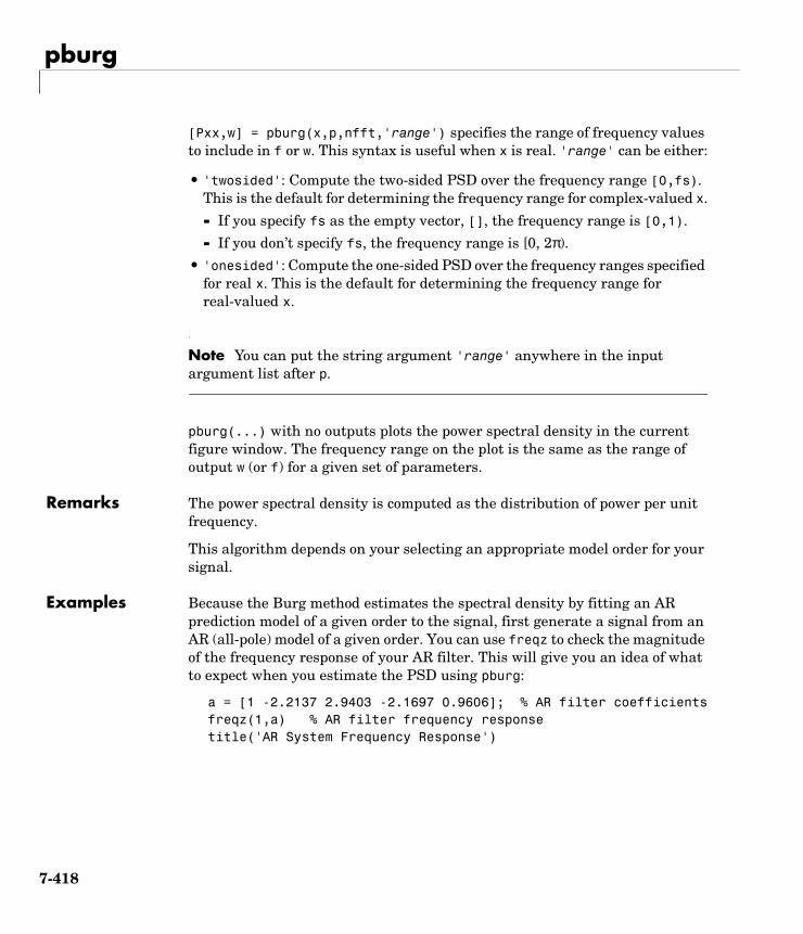
pburg
[Pxx,w] = pburg(x,p,nfft,'range') specifies the range of frequency values to include in f or w. This syntax is useful when x is real. 'range' can be either:
• 'twosided': Compute the two-sided PSD over the frequency range [0,fs). This is the default for determining the frequency range for complex-valued x.
- If you specify fs as the empty vector, [], the frequency range is [0,1).
- If you don’t specify fs, the frequency range is [0, 2π).
• 'onesided': Compute the one-sided PSD over the frequency ranges specified for real x. This is the default for determining the frequency range for real-valued x.
Note You can put the string argument 'range' anywhere in the input argument list after p.
pburg(...) with no outputs plots the power spectral density in the current figure window. The frequency range on the plot is the same as the range of output w (or f) for a given set of parameters.
Remarks The power spectral density is computed as the distribution of power per unit frequency.
This algorithm depends on your selecting an appropriate model order for your signal.
Examples Because the Burg method estimates the spectral density by fitting an AR prediction model of a given order to the signal, first generate a signal from an AR (all-pole) model of a given order. You can use freqz to check the magnitude of the frequency response of your AR filter. This will give you an idea of what to expect when you estimate the PSD using pburg:
a = [1 -2.2137 2.9403 -2.1697 0.9606]; % AR filter coefficientsfreqz(1,a) % AR filter frequency responsetitle('AR System Frequency Response')
7-418
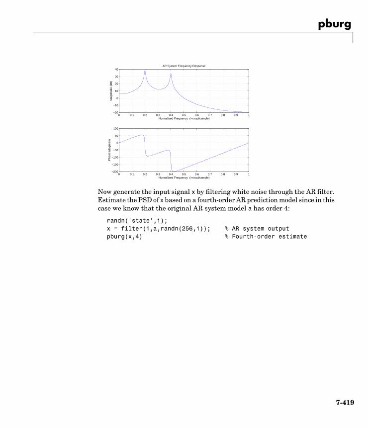
pburg
Now generate the input signal x by filtering white noise through the AR filter. Estimate the PSD of x based on a fourth-order AR prediction model since in this case we know that the original AR system model a has order 4:
randn('state',1);x = filter(1,a,randn(256,1)); % AR system outputpburg(x,4) % Fourth-order estimate
0 0.1 0.2 0.3 0.4 0.5 0.6 0.7 0.8 0.9 1−200
−150
−100
−50
0
50
100
Normalized Frequency (×π rad/sample)
Pha
se (
degr
ees)
0 0.1 0.2 0.3 0.4 0.5 0.6 0.7 0.8 0.9 1−20
−10
0
10
20
30
40
Normalized Frequency (×π rad/sample)
Mag
nitu
de (
dB)
AR System Frequency Response
7-419
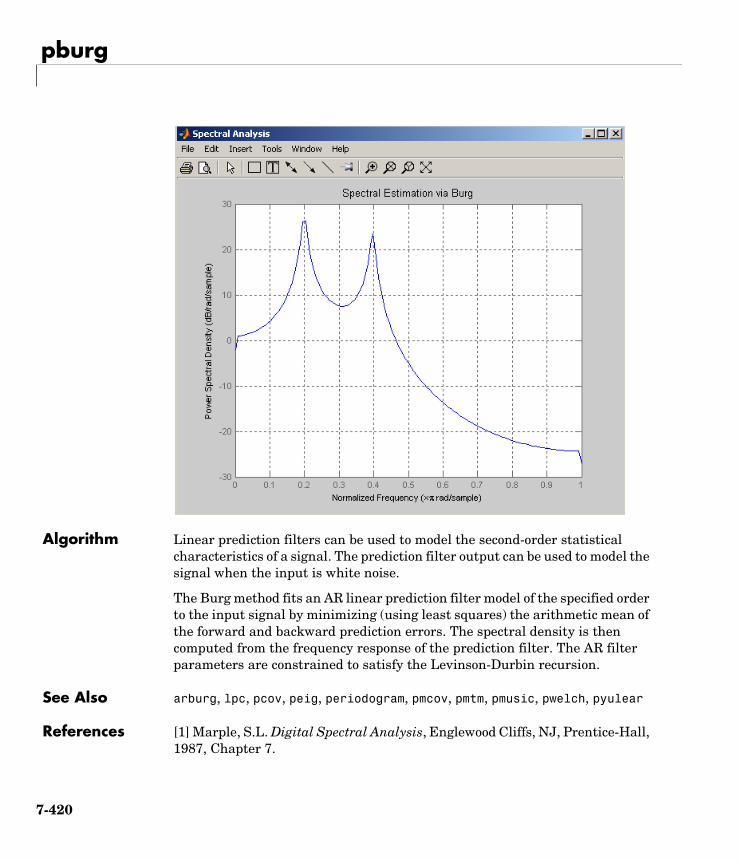
pburg
Algorithm Linear prediction filters can be used to model the second-order statistical characteristics of a signal. The prediction filter output can be used to model the signal when the input is white noise.
The Burg method fits an AR linear prediction filter model of the specified order to the input signal by minimizing (using least squares) the arithmetic mean of the forward and backward prediction errors. The spectral density is then computed from the frequency response of the prediction filter. The AR filter parameters are constrained to satisfy the Levinson-Durbin recursion.
See Also arburg, lpc, pcov, peig, periodogram, pmcov, pmtm, pmusic, pwelch, pyulear
References [1] Marple, S.L. Digital Spectral Analysis, Englewood Cliffs, NJ, Prentice-Hall, 1987, Chapter 7.
7-420

pburg
[2] Stoica, P., and R.L. Moses, Introduction to Spectral Analysis, Prentice-Hall, 1997.
7-421
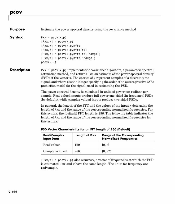
pcov
7pcovPurpose Estimate the power spectral density using the covariance method
Syntax Pxx = pcov(x,p)[Pxx,w] = pcov(x,p)[Pxx,w] = pcov(x,p,nfft)[Pxx,f] = pcov(x,p,nfft,fs)[Pxx,f] = pcov(x,p,nfft,fs,'range')[Pxx,w] = pcov(x,p,nfft,'range')pcov(...)
Description Pxx = pcov(x,p) implements the covariance algorithm, a parametric spectral estimation method, and returns Pxx, an estimate of the power spectral density (PSD) of the vector x. The entries of x represent samples of a discrete-time signal, and where p is the integer specifying the order of an autoregressive (AR) prediction model for the signal, used in estimating the PSD.
The power spectral density is calculated in units of power per radians per sample. Real-valued inputs produce full power one-sided (in frequency) PSDs (by default), while complex-valued inputs produce two-sided PSDs.
In general, the length of the FFT and the values of the input x determine the length of Pxx and the range of the corresponding normalized frequencies. For this syntax, the (default) FFT length is 256. The following table indicates the length of Pxx and the range of the corresponding normalized frequencies for this syntax.
[Pxx,w] = pcov(x,p) also returns w, a vector of frequencies at which the PSD is estimated. Pxx and w have the same length. The units for frequency are rad/sample.
PSD Vector Characteristics for an FFT Length of 256 (Default)
Real/Complex Input Data
Length of Pxx Range of the Corresponding Normalized Frequencies
Real-valued 129 [0, π]
Complex-valued 256 [0, 2π)
7-422
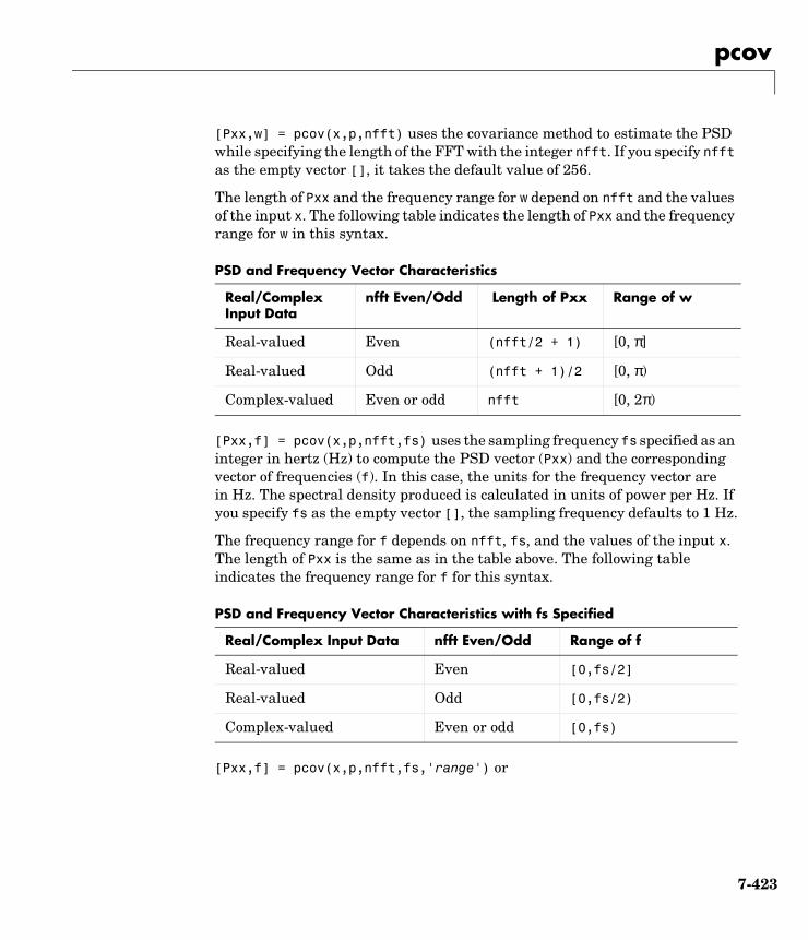
pcov
[Pxx,w] = pcov(x,p,nfft) uses the covariance method to estimate the PSD while specifying the length of the FFT with the integer nfft. If you specify nfft as the empty vector [], it takes the default value of 256.
The length of Pxx and the frequency range for w depend on nfft and the values of the input x. The following table indicates the length of Pxx and the frequency range for w in this syntax.
[Pxx,f] = pcov(x,p,nfft,fs) uses the sampling frequency fs specified as an integer in hertz (Hz) to compute the PSD vector (Pxx) and the corresponding vector of frequencies (f). In this case, the units for the frequency vector are in Hz. The spectral density produced is calculated in units of power per Hz. If you specify fs as the empty vector [], the sampling frequency defaults to 1 Hz.
The frequency range for f depends on nfft, fs, and the values of the input x. The length of Pxx is the same as in the table above. The following table indicates the frequency range for f for this syntax.
[Pxx,f] = pcov(x,p,nfft,fs,'range') or
PSD and Frequency Vector Characteristics
Real/Complex Input Data
nfft Even/Odd Length of Pxx Range of w
Real-valued Even (nfft/2 + 1) [0, π]
Real-valued Odd (nfft + 1)/2 [0, π)
Complex-valued Even or odd nfft [0, 2π)
PSD and Frequency Vector Characteristics with fs Specified
Real/Complex Input Data nfft Even/Odd Range of f
Real-valued Even [0,fs/2]
Real-valued Odd [0,fs/2)
Complex-valued Even or odd [0,fs)
7-423
pcov
[Pxx,w] = pcov(x,p,nfft,'range') specifies the range of frequency values to include in f or w. This syntax is useful when x is real. 'range' can be either:
• 'twosided': Compute the two-sided PSD over the frequency range [0,fs). This is the default for determining the frequency range for complex-valued x.
- If you specify fs as the empty vector, [], the frequency range is [0,1).
- If you don’t specify fs, the frequency range is [0, 2π).
• 'onesided': Compute the one-sided PSD over the frequency ranges specified for real x. This is the default for determining the frequency range for real-valued x.
Note You can put the string argument 'range' anywhere in the input argument list after p.
pcov(...) with no outputs plots the power spectral density in the current figure window. The frequency range on the plot is the same as the range of output w (or f) for a given set of parameters.
Remarks The power spectral density is computed as the distribution of power per unit frequency.
This algorithm depends on your selecting an appropriate model order for your signal.
Examples Because the covariance method estimates the spectral density by fitting an AR prediction model of a given order to the signal, first generate a signal from an AR (all-pole) model of a given order. You can use freqz to check the magnitude of the frequency response of your AR filter. This will give you an idea of what to expect when you estimate the PSD using pcov:
a = [1 -2.2137 2.9403 -2.1697 0.9606]; % AR filter coefficientsfreqz(1,a) % AR filter frequency responsetitle('AR System Frequency Response')
7-424
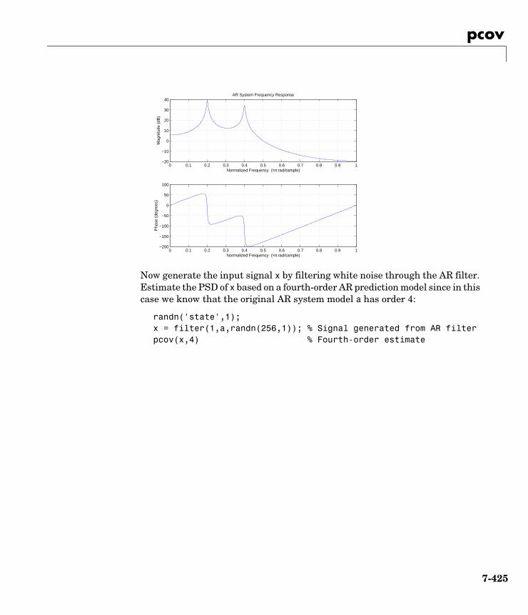
pcov
Now generate the input signal x by filtering white noise through the AR filter. Estimate the PSD of x based on a fourth-order AR prediction model since in this case we know that the original AR system model a has order 4:
randn('state',1);x = filter(1,a,randn(256,1)); % Signal generated from AR filter pcov(x,4) % Fourth-order estimate
0 0.1 0.2 0.3 0.4 0.5 0.6 0.7 0.8 0.9 1−200
−150
−100
−50
0
50
100
Normalized Frequency (×π rad/sample)
Pha
se (
degr
ees)
0 0.1 0.2 0.3 0.4 0.5 0.6 0.7 0.8 0.9 1−20
−10
0
10
20
30
40
Normalized Frequency (×π rad/sample)
Mag
nitu
de (
dB)
AR System Frequency Response
7-425
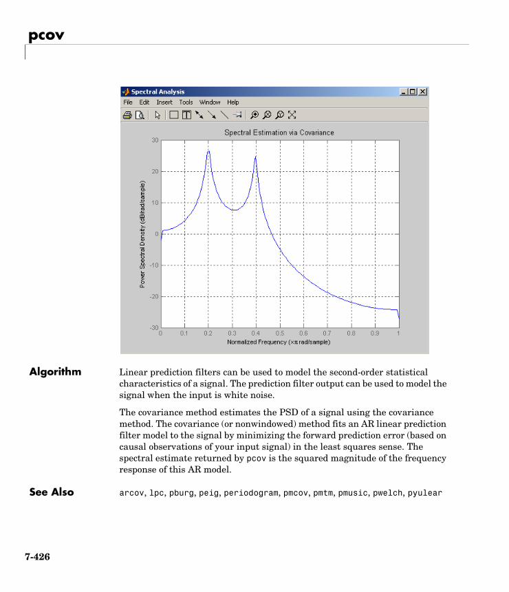
pcov
Algorithm Linear prediction filters can be used to model the second-order statistical characteristics of a signal. The prediction filter output can be used to model the signal when the input is white noise.
The covariance method estimates the PSD of a signal using the covariance method. The covariance (or nonwindowed) method fits an AR linear prediction filter model to the signal by minimizing the forward prediction error (based on causal observations of your input signal) in the least squares sense. The spectral estimate returned by pcov is the squared magnitude of the frequency response of this AR model.
See Also arcov, lpc, pburg, peig, periodogram, pmcov, pmtm, pmusic, pwelch, pyulear
7-426

pcov
References [1] Marple, S.L. Digital Spectral Analysis, Englewood Cliffs, NJ, Prentice-Hall, 1987, Chapter 7.
[2] Stoica, P., and R.L. Moses, Introduction to Spectral Analysis, Prentice-Hall, 1997.
7-427
peig
7peigPurpose Estimate the pseudospectrum using the eigenvector method
Syntax [S,w] = peig(x,p)[S,w] = peig(...,nfft)[S,f] = peig(x,p,nfft,fs)[S,f] = peig(...,'corr')[S,f] = peig(x,p,nfft,fs,nwin,noverlap)[...] = peig(...,'range')[...,v,e] = peig(...)peig(...)
Description [S,w] = peig(x,p) implements the eigenvector spectral estimation method and returns S, the pseudospectrum estimate of the input signal x, and w, a vector of normalized frequencies (in rad/sample) at which the pseudospectrum is evaluated. The pseudospectrum is calculated using estimates of the eigenvectors of a correlation matrix associated with the input data x, where x is specified as either:
• A row or column vector representing one observation of the signal
• A rectangular array for which each row of x represents a separate observation of the signal (for example, each row is one output of an array of sensors, as in array processing), such that x'*x is an estimate of the correlation matrix
Note You can use the output of corrmtx to generate such an array x.
You can specify the second input argument p as either:
• A scalar integer. In this case, the signal subspace dimension is p.
• A two-element vector. In this case, p(2), the second element of p, represents a threshold that is multiplied by λmin, the smallest estimated eigenvalue of the signal’s correlation matrix. Eigenvalues below the threshold λmin*p(2) are assigned to the noise subspace. In this case, p(1) specifies the maximum dimension of the signal subspace.
7-428
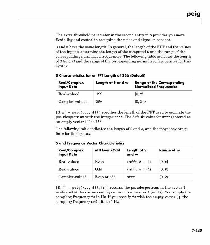
peig
The extra threshold parameter in the second entry in p provides you more flexibility and control in assigning the noise and signal subspaces.
S and w have the same length. In general, the length of the FFT and the values of the input x determine the length of the computed S and the range of the corresponding normalized frequencies. The following table indicates the length of S (and w) and the range of the corresponding normalized frequencies for this syntax.
[S,w] = peig(...,nfft) specifies the length of the FFT used to estimate the pseudospectrum with the integer nfft. The default value for nfft (entered as an empty vector []) is 256.
The following table indicates the length of S and w, and the frequency range for w for this syntax.
[S,f] = peig(x,p,nfft,fs)) returns the pseudospectrum in the vector S evaluated at the corresponding vector of frequencies f (in Hz). You supply the sampling frequency fs in Hz. If you specify fs with the empty vector [], the sampling frequency defaults to 1 Hz.
S Characteristics for an FFT Length of 256 (Default)
Real/Complex Input Data
Length of S and w Range of the Corresponding Normalized Frequencies
Real-valued 129 [0, π]
Complex-valued 256 [0, 2π)
S and Frequency Vector Characteristics
Real/Complex Input Data
nfft Even/Odd Length of S and w
Range of w
Real-valued Even (nfft/2 + 1) [0, π]
Real-valued Odd (nfft + 1)/2 [0, π)
Complex-valued Even or odd nfft [0, 2π)
7-429
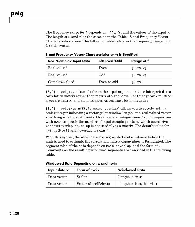
peig
The frequency range for f depends on nfft, fs, and the values of the input x. The length of S (and f) is the same as in the Table , S and Frequency Vector Characteristics above. The following table indicates the frequency range for f for this syntax.
[S,f] = peig(...,'corr') forces the input argument x to be interpreted as a correlation matrix rather than matrix of signal data. For this syntax x must be a square matrix, and all of its eigenvalues must be nonnegative.
[S,f] = peig(x,p,nfft,fs,nwin,noverlap) allows you to specify nwin, a scalar integer indicating a rectangular window length, or a real-valued vector specifying window coefficients. Use the scalar integer noverlap in conjunction with nwin to specify the number of input sample points by which successive windows overlap. noverlap is not used if x is a matrix. The default value for nwin is 2*p(1) and noverlap is nwin-1.
With this syntax, the input data x is segmented and windowed before the matrix used to estimate the correlation matrix eigenvalues is formulated. The segmentation of the data depends on nwin, noverlap, and the form of x. Comments on the resulting windowed segments are described in the following table.
S and Frequency Vector Characteristics with fs Specified
Real/Complex Input Data nfft Even/Odd Range of f
Real-valued Even [0,fs/2]
Real-valued Odd [0,fs/2)
Complex-valued Even or odd [0,fs)
Windowed Data Depending on x and nwin
Input data x Form of nwin Windowed Data
Data vector Scalar Length is nwin
Data vector Vector of coefficients Length is length(nwin)
7-430
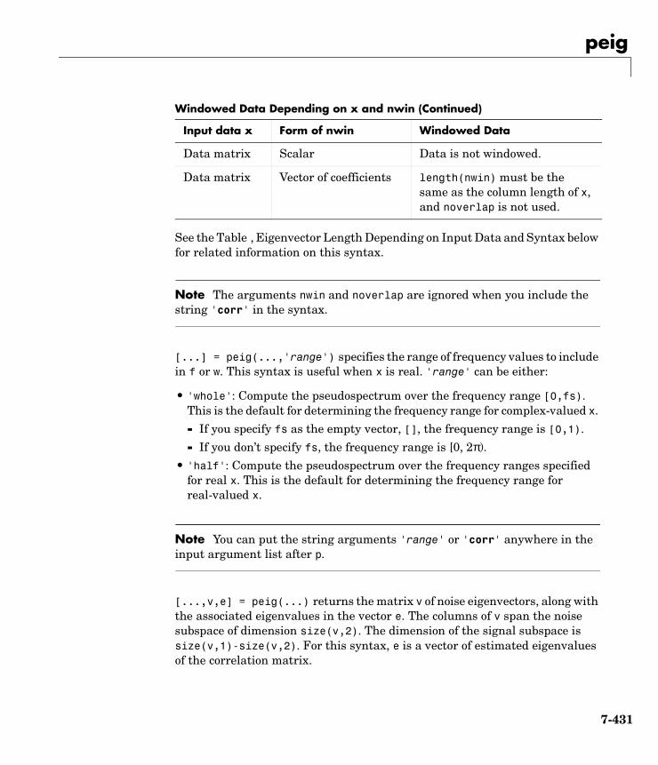
peig
See the Table , Eigenvector Length Depending on Input Data and Syntax below for related information on this syntax.
Note The arguments nwin and noverlap are ignored when you include the string 'corr' in the syntax.
[...] = peig(...,'range') specifies the range of frequency values to include in f or w. This syntax is useful when x is real. 'range' can be either:
• 'whole': Compute the pseudospectrum over the frequency range [0,fs). This is the default for determining the frequency range for complex-valued x.
- If you specify fs as the empty vector, [], the frequency range is [0,1).
- If you don’t specify fs, the frequency range is [0, 2π).
• 'half': Compute the pseudospectrum over the frequency ranges specified for real x. This is the default for determining the frequency range for real-valued x.
Note You can put the string arguments 'range' or 'corr' anywhere in the input argument list after p.
[...,v,e] = peig(...) returns the matrix v of noise eigenvectors, along with the associated eigenvalues in the vector e. The columns of v span the noise subspace of dimension size(v,2). The dimension of the signal subspace is size(v,1)-size(v,2). For this syntax, e is a vector of estimated eigenvalues of the correlation matrix.
Data matrix Scalar Data is not windowed.
Data matrix Vector of coefficients length(nwin) must be the same as the column length of x, and noverlap is not used.
Windowed Data Depending on x and nwin (Continued)
Input data x Form of nwin Windowed Data
7-431
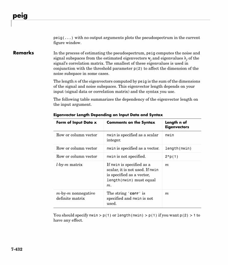
peig
peig(...) with no output arguments plots the pseudospectrum in the current figure window.
Remarks In the process of estimating the pseudospectrum, peig computes the noise and signal subspaces from the estimated eigenvectors vj and eigenvalues λj of the signal’s correlation matrix. The smallest of these eigenvalues is used in conjunction with the threshold parameter p(2) to affect the dimension of the noise subspace in some cases.
The length n of the eigenvectors computed by peig is the sum of the dimensions of the signal and noise subspaces. This eigenvector length depends on your input (signal data or correlation matrix) and the syntax you use.
The following table summarizes the dependency of the eigenvector length on the input argument.
You should specify nwin > p(1) or length(nwin) > p(1) if you want p(2) > 1 to have any effect.
Eigenvector Length Depending on Input Data and Syntax
Form of Input Data x Comments on the Syntax Length n of Eigenvectors
Row or column vector nwin is specified as a scalar integer.
nwin
Row or column vector nwin is specified as a vector. length(nwin)
Row or column vector nwin is not specified. 2*p(1)
l-by-m matrix If nwin is specified as a scalar, it is not used. If nwin is specified as a vector, length(nwin) must equal m.
m
m-by-m nonnegative definite matrix
The string 'corr' is specified and nwin is not used.
m
7-432
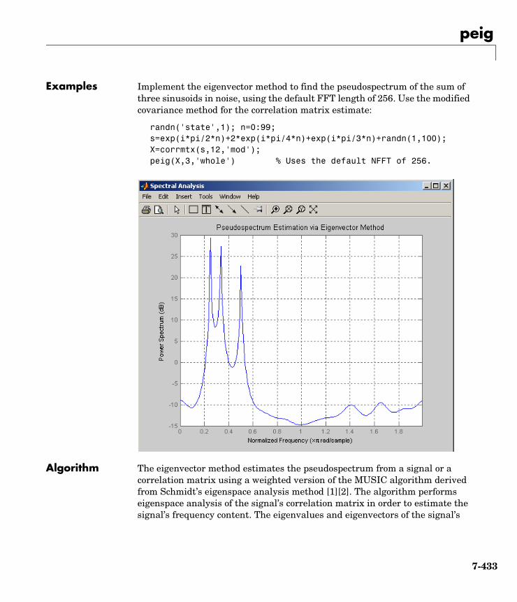
peig
Examples Implement the eigenvector method to find the pseudospectrum of the sum of three sinusoids in noise, using the default FFT length of 256. Use the modified covariance method for the correlation matrix estimate:
randn('state',1); n=0:99; s=exp(i*pi/2*n)+2*exp(i*pi/4*n)+exp(i*pi/3*n)+randn(1,100); X=corrmtx(s,12,'mod'); peig(X,3,'whole') % Uses the default NFFT of 256.
Algorithm The eigenvector method estimates the pseudospectrum from a signal or a correlation matrix using a weighted version of the MUSIC algorithm derived from Schmidt’s eigenspace analysis method [1][2]. The algorithm performs eigenspace analysis of the signal’s correlation matrix in order to estimate the signal’s frequency content. The eigenvalues and eigenvectors of the signal’s
7-433
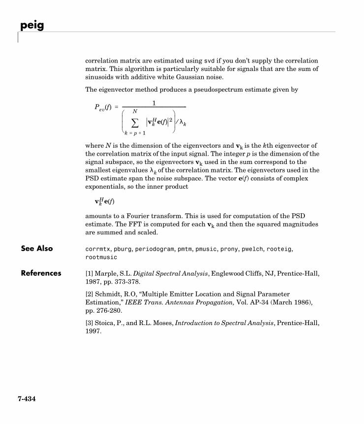
peig
correlation matrix are estimated using svd if you don’t supply the correlation matrix. This algorithm is particularly suitable for signals that are the sum of sinusoids with additive white Gaussian noise.
The eigenvector method produces a pseudospectrum estimate given by
where N is the dimension of the eigenvectors and vk is the kth eigenvector of the correlation matrix of the input signal. The integer p is the dimension of the signal subspace, so the eigenvectors vk used in the sum correspond to the smallest eigenvalues of the correlation matrix. The eigenvectors used in the PSD estimate span the noise subspace. The vector e(f) consists of complex exponentials, so the inner product
amounts to a Fourier transform. This is used for computation of the PSD estimate. The FFT is computed for each vk and then the squared magnitudes are summed and scaled.
See Also corrmtx, pburg, periodogram, pmtm, pmusic, prony, pwelch, rooteig, rootmusic
References [1] Marple, S.L. Digital Spectral Analysis, Englewood Cliffs, NJ, Prentice-Hall, 1987, pp. 373-378.
[2] Schmidt, R.O, “Multiple Emitter Location and Signal Parameter Estimation,” IEEE Trans. Antennas Propagation, Vol. AP-34 (March 1986), pp. 276-280.
[3] Stoica, P., and R.L. Moses, Introduction to Spectral Analysis, Prentice-Hall, 1997.
Pev f( )1
vkHe f( ) 2
k p 1+=
N
∑
λk⁄
-----------------------------------------------------------=
λk
vkHe f( )
7-434
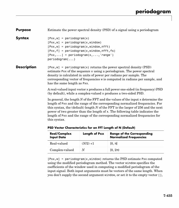
periodogram
7periodogramPurpose Estimate the power spectral density (PSD) of a signal using a periodogram
Syntax [Pxx,w] = periodogram(x)[Pxx,w] = periodogram(x,window)[Pxx,w] = periodogram(x,window,nfft)[Pxx,f] = periodogram(x,window,nfft,fs)[Pxx,...] = periodogram(x,...,'range')periodogram(...)
Description [Pxx,w] = periodogram(x) returns the power spectral density (PSD) estimate Pxx of the sequence x using a periodogram. The power spectral density is calculated in units of power per radians per sample. The corresponding vector of frequencies w is computed in radians per sample, and has the same length as Pxx.
A real-valued input vector x produces a full power one-sided (in frequency) PSD (by default), while a complex-valued x produces a two-sided PSD.
In general, the length N of the FFT and the values of the input x determine the length of Pxx and the range of the corresponding normalized frequencies. For this syntax, the (default) length N of the FFT is the larger of 256 and the next power of two greater than the length of x. The following table indicates the length of Pxx and the range of the corresponding normalized frequencies for this syntax.
[Pxx,w] = periodogram(x,window) returns the PSD estimate Pxx computed using the modified periodogram method. The vector window specifies the coefficients of the window used in computing a modified periodogram of the input signal. Both input arguments must be vectors of the same length. When you don’t supply the second argument window, or set it to the empty vector [],
PSD Vector Characteristics for an FFT Length of N (Default)
Real/Complex Input Data
Length of Pxx Range of the Corresponding Normalized Frequencies
Real-valued (N/2) +1 [0, π]
Complex-valued N [0, 2π)
7-435
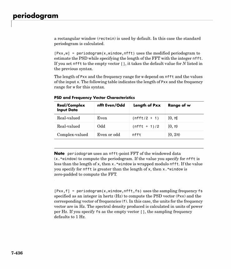
periodogram
a rectangular window (rectwin) is used by default. In this case the standard periodogram is calculated.
[Pxx,w] = periodogram(x,window,nfft) uses the modified periodogram to estimate the PSD while specifying the length of the FFT with the integer nfft. If you set nfft to the empty vector [], it takes the default value for N listed in the previous syntax.
The length of Pxx and the frequency range for w depend on nfft and the values of the input x. The following table indicates the length of Pxx and the frequency range for w for this syntax.
Note periodogram uses an nfft-point FFT of the windowed data (x.*window) to compute the periodogram. If the value you specify for nfft is less than the length of x, then x.*window is wrapped modulo nfft. If the value you specify for nfft is greater than the length of x, then x.*window is zero-padded to compute the FFT.
[Pxx,f] = periodogram(x,window,nfft,fs) uses the sampling frequency fs specified as an integer in hertz (Hz) to compute the PSD vector (Pxx) and the corresponding vector of frequencies (f). In this case, the units for the frequency vector are in Hz. The spectral density produced is calculated in units of power per Hz. If you specify fs as the empty vector [], the sampling frequency defaults to 1 Hz.
PSD and Frequency Vector Characteristics
Real/Complex Input Data
nfft Even/Odd Length of Pxx Range of w
Real-valued Even (nfft/2 + 1) [0, π]
Real-valued Odd (nfft + 1)/2 [0, π)
Complex-valued Even or odd nfft [0, 2π)
7-436
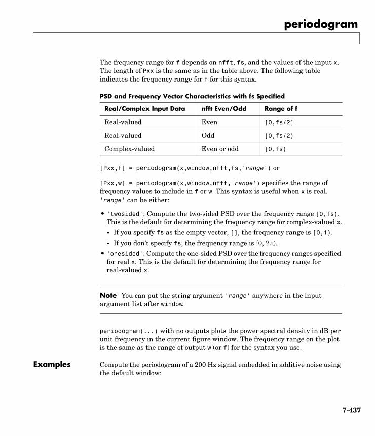
periodogram
The frequency range for f depends on nfft, fs, and the values of the input x. The length of Pxx is the same as in the table above. The following table indicates the frequency range for f for this syntax.
[Pxx,f] = periodogram(x,window,nfft,fs,'range') or
[Pxx,w] = periodogram(x,window,nfft,'range') specifies the range of frequency values to include in f or w. This syntax is useful when x is real. 'range' can be either:
• 'twosided': Compute the two-sided PSD over the frequency range [0,fs). This is the default for determining the frequency range for complex-valued x.
- If you specify fs as the empty vector, [], the frequency range is [0,1).
- If you don’t specify fs, the frequency range is [0, 2π).
• 'onesided': Compute the one-sided PSD over the frequency ranges specified for real x. This is the default for determining the frequency range for real-valued x.
Note You can put the string argument 'range' anywhere in the input argument list after window.
periodogram(...) with no outputs plots the power spectral density in dB per unit frequency in the current figure window. The frequency range on the plot is the same as the range of output w (or f) for the syntax you use.
Examples Compute the periodogram of a 200 Hz signal embedded in additive noise using the default window:
PSD and Frequency Vector Characteristics with fs Specified
Real/Complex Input Data nfft Even/Odd Range of f
Real-valued Even [0,fs/2]
Real-valued Odd [0,fs/2)
Complex-valued Even or odd [0,fs)
7-437
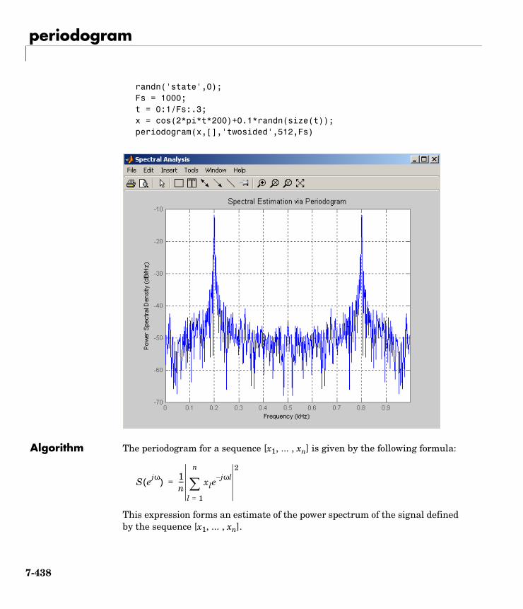
periodogram
randn('state',0);Fs = 1000; t = 0:1/Fs:.3;x = cos(2*pi*t*200)+0.1*randn(size(t)); periodogram(x,[],'twosided',512,Fs)
Algorithm The periodogram for a sequence [x1, ... , xn] is given by the following formula:
This expression forms an estimate of the power spectrum of the signal defined by the sequence [x1, ... , xn].
S ejω( ) 1n--- xle
jωl–
l 1=
n
∑2
=
7-438
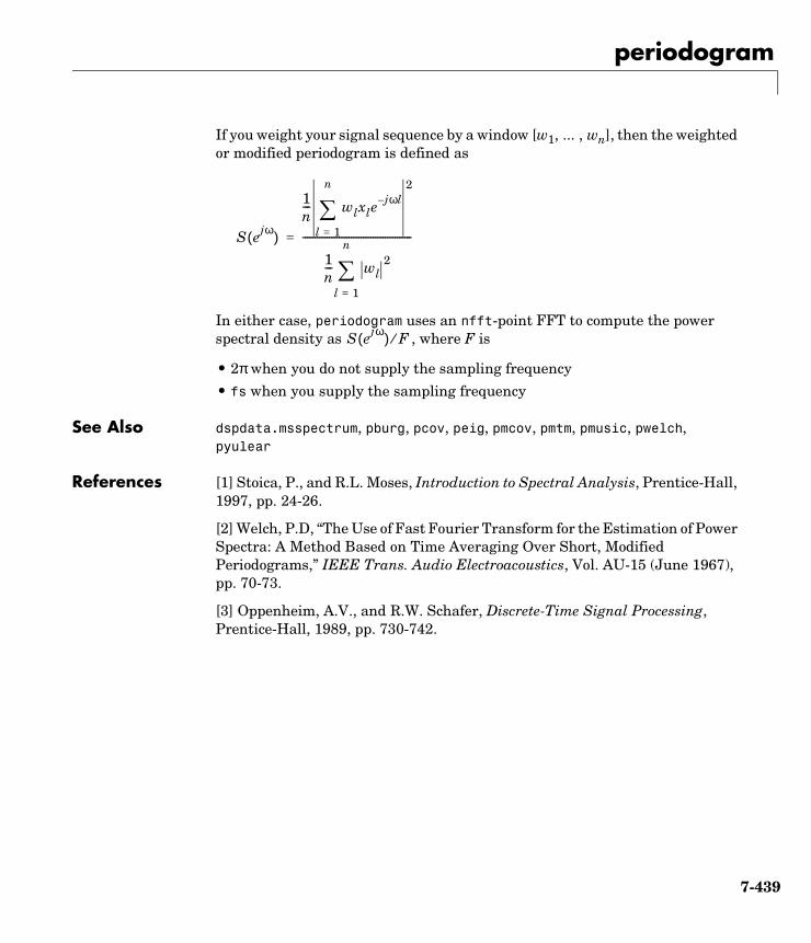
periodogram
If you weight your signal sequence by a window [w1, ... , wn], then the weighted or modified periodogram is defined as
In either case, periodogram uses an nfft-point FFT to compute the power spectral density as , where F is
• 2π when you do not supply the sampling frequency
• fs when you supply the sampling frequency
See Also dspdata.msspectrum, pburg, pcov, peig, pmcov, pmtm, pmusic, pwelch, pyulear
References [1] Stoica, P., and R.L. Moses, Introduction to Spectral Analysis, Prentice-Hall, 1997, pp. 24-26.
[2] Welch, P.D, “The Use of Fast Fourier Transform for the Estimation of Power Spectra: A Method Based on Time Averaging Over Short, Modified Periodograms,” IEEE Trans. Audio Electroacoustics, Vol. AU-15 (June 1967), pp. 70-73.
[3] Oppenheim, A.V., and R.W. Schafer, Discrete-Time Signal Processing, Prentice-Hall, 1989, pp. 730-742.
S ejω( )
1n--- wlxle
jωl–
l 1=
n
∑2
1n--- wl
2
l 1=
n
∑
---------------------------------------------=
S ejω( ) F⁄
7-439
phasedelay
7phasedelayPurpose Compute the phase delay of a digital filter
Syntax [phi,w] = phasedelay(b,a,n)[phi,w] = phasedelay(b,a,n,'whole')phi = phasedelay(b,a,w)[phi,f] = phasedelay(b,a,n,fs)[phi,f] = phasedelay(b,a,n,'whole',fs)phi = phasedelay(b,a,f,fs)[phi,w,s] = phasedelay(...)[phi,f,s] = phasedelay(...)phasedelay(b,a,...)
Description [phi,w] = phasedelay(b,a,n) returns the n-point phase delay response vector phi and the n-point frequency reponse vector w (in radians/sample) of the filter defined by numerator coefficients b and denominator coefficients a. The phase delay response is evaluated at n equally spaced points around the upper half of the unit circle. If n is omitted, it defaults to 512.
[phi,w] = phasedelay(b,a,n,'whole') uses n equally spaced points around the whole unit circle.
phi = phasedelay(b,a,w) returns the phase delay response at frequencies specified in vector w (in radians/sample). The frequencies are normally between 0 and π.
[phi,f] = phasedelay(b,a,n,fs) and [phi,f] = phasedelay(b,a,n,'whole',fs) return the phase delay vector f (in Hz), using the sampling frequency fs (in Hz).
phi = phasedelay(b,a,f,fs) returns the phase delay response at the frequencies specified in vector f (in Hz), using the sampling frequency fs (in Hz)..
[phi,w,s] = phasedelay(...) and [phi,f,s] = phasedelay(...) return plotting information, where s is a structure with fields you can change to display different frequency response plots.
phasedelay(b,a,...) with no output arguments, plots the phase delay response of the filter.
7-440
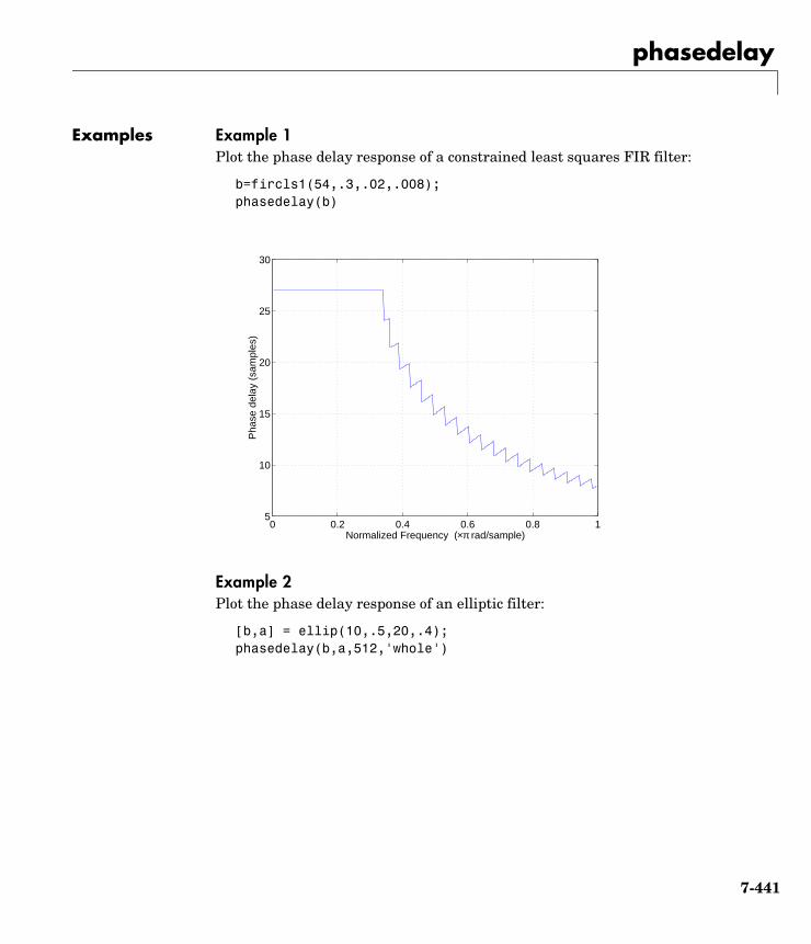
phasedelay
Examples Example 1Plot the phase delay response of a constrained least squares FIR filter:
b=fircls1(54,.3,.02,.008); phasedelay(b)
Example 2Plot the phase delay response of an elliptic filter:
[b,a] = ellip(10,.5,20,.4); phasedelay(b,a,512,'whole')
0 0.2 0.4 0.6 0.8 15
10
15
20
25
30
Normalized Frequency (×π rad/sample)
Pha
se d
elay
(sa
mpl
es)
7-441
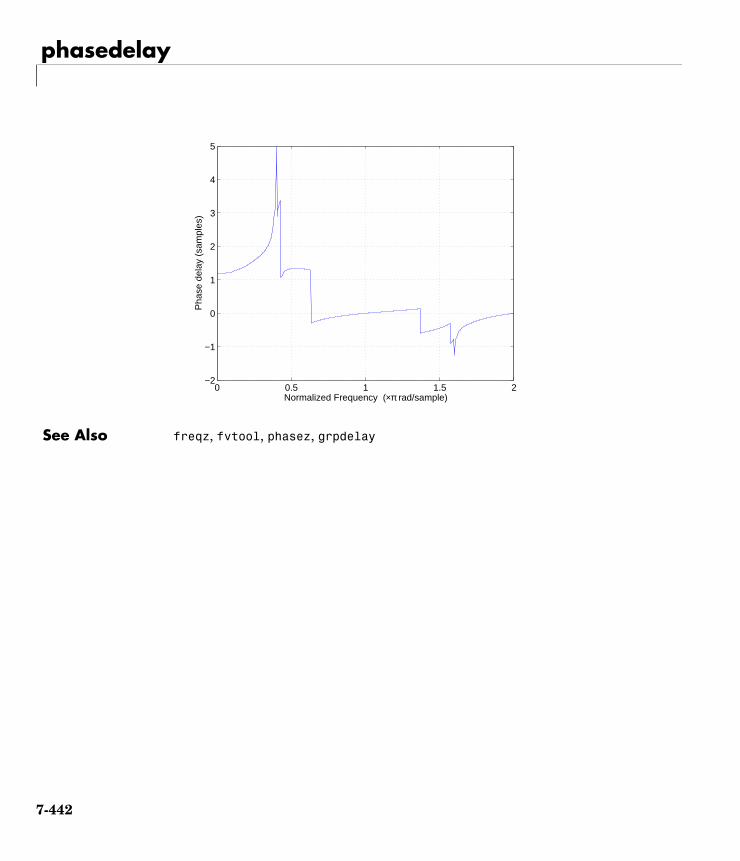
phasedelay
See Also freqz, fvtool, phasez, grpdelay
0 0.5 1 1.5 2−2
−1
0
1
2
3
4
5
Normalized Frequency (×π rad/sample)
Pha
se d
elay
(sa
mpl
es)
7-442
phasez
7phasezPurpose Compute the phase response of a digital filter
Syntax [phi,w] = phasez(b,a,n)[phi,w] = phasez(b,a,n,'whole')phi = phasez(b,a,w)[phi,f] = phasez(b,a,n,fs)[phi,f] = phasez(b,a,n,'whole',fs)phi = phasez(b,a,f,fs)[phi,w,s] = phasez(...)[phi,f,s] = phasez(...)phasez(b,a,...)phasez(Hd)
Description [phi,w] = phasez(b,a,n) returns the n-point phase response vector phi and the n-point frequency reponse vector w (in radians/sample) of the filter defined by numerator coefficients b and denominator coefficients a. The phase response is evaluated at n equally spaced points around the upper half of the unit circle. If n is omitted, it defaults to 512.
[phi,w] = phasez(b,a,n,'whole') uses n equally spaced points around the whole unit circle.
phi = phasez(b,a,w) returns the phase response at frequencies specified in vector w (in radians/sample). The frequencies are normally between 0 and π.
[phi,f] = phasez(b,a,n,fs) and [phi,f] = phasez(b,a,n,'whole',fs) return the phase vector f (in Hz), using the sampling frequency fs (in Hz).
phi = phasez(b,a,f,fs) returns the phase response at the frequencies specified in vector f (in Hz), using the sampling frequency fs (in Hz)..
[phi,w,s] = phasez(...) and [phi,f,s] = phasez(...) return plotting information, where s is a structure with fields you can change to display different frequency response plots.
phasez(b,a,...) with no output arguments, plots the phase response of the filter in the current filter window.
7-443
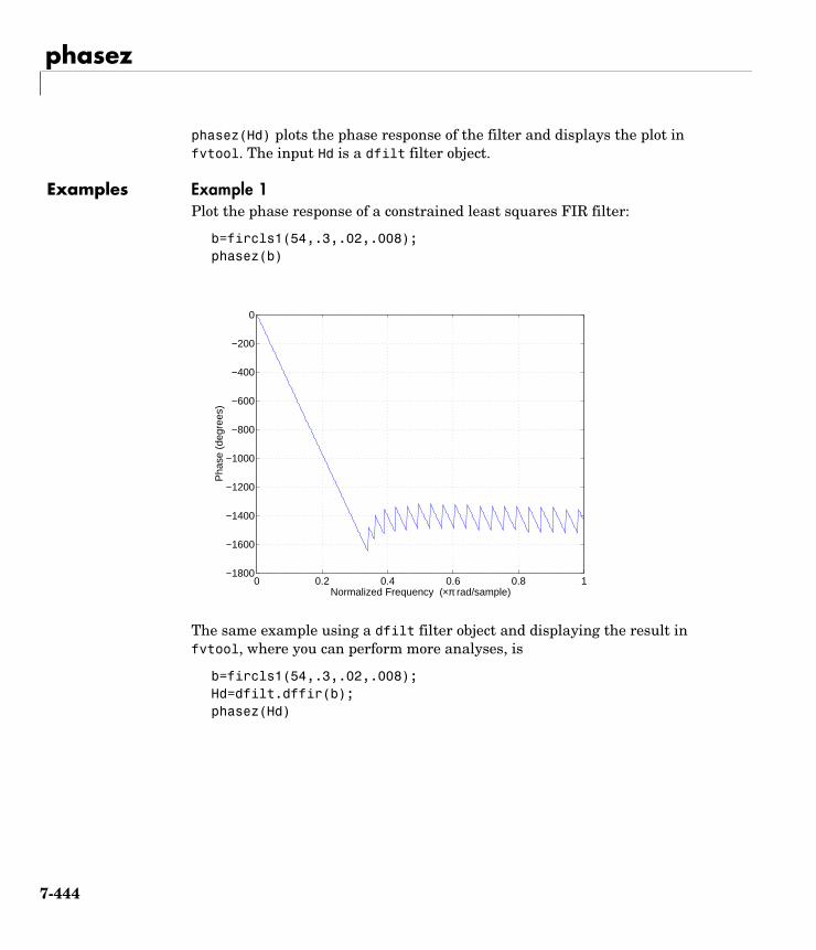
phasez
phasez(Hd) plots the phase response of the filter and displays the plot in fvtool. The input Hd is a dfilt filter object.
Examples Example 1Plot the phase response of a constrained least squares FIR filter:
b=fircls1(54,.3,.02,.008); phasez(b)
The same example using a dfilt filter object and displaying the result in fvtool, where you can perform more analyses, is
b=fircls1(54,.3,.02,.008); Hd=dfilt.dffir(b);phasez(Hd)
0 0.2 0.4 0.6 0.8 1−1800
−1600
−1400
−1200
−1000
−800
−600
−400
−200
0
Normalized Frequency (×π rad/sample)
Pha
se (
degr
ees)
7-444
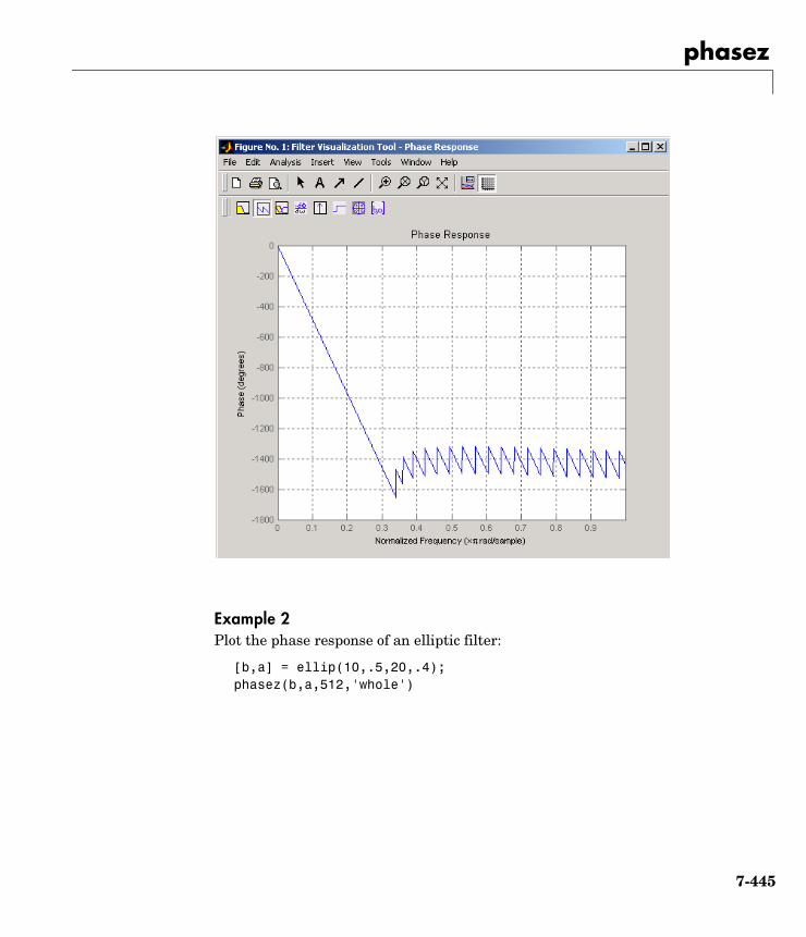
phasez
Example 2Plot the phase response of an elliptic filter:
[b,a] = ellip(10,.5,20,.4); phasez(b,a,512,'whole')
7-445
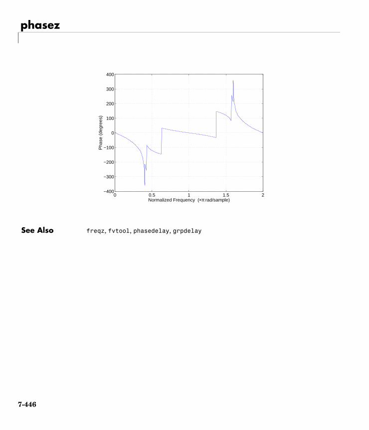
phasez
See Also freqz, fvtool, phasedelay, grpdelay
0 0.5 1 1.5 2−400
−300
−200
−100
0
100
200
300
400
Normalized Frequency (×π rad/sample)
Pha
se (
degr
ees)
7-446
pmcov
7pmcovPurpose Estimate the power spectral density using the modified covariance method
Syntax Pxx = pmcov(x,p)[Pxx,w] = pmcov(x,p)[Pxx,w] = pmcov(x,p,nfft)[Pxx,f] = pmcov(x,p,nfft,fs)[Pxx,f] = pmcov(x,p,nfft,fs,'range')[Pxx,w] = pmcov(x,p,nfft,'range')pmcov(...)
Description Pxx = pmcov(x,p) implements the modified covariance algorithm, a parametric spectral estimation method, and returns Pxx, an estimate of the power spectral density (PSD) of the vector x. The entries of x represent samples of a discrete-time signal, and p is the integer specifying the order of an autoregressive (AR) prediction model for the signal, used in estimating the PSD.
The power spectral density is calculated in units of power per radians per sample. Real-valued inputs produce full power one-sided (in frequency) PSDs (by default), while complex-valued inputs produce two-sided PSDs.
In general, the length of the FFT and the values of the input x determine the length of Pxx and the range of the corresponding normalized frequencies. For this syntax, the (default) FFT length is 256. The following table indicates the length of Pxx and the range of the corresponding normalized frequencies for this syntax.
[Pxx,w] = pmcov(x,p) also returns w, a vector of frequencies at which the PSD is estimated. Pxx and w have the same length. The units for frequency are rad/sample.
PSD Vector Characteristics for an FFT Length of 256 (Default)
Real/Complex Input Data
Length of Pxx Range of the Corresponding Normalized Frequencies
Real-valued 129 [0, π]
Complex-valued 256 [0, 2π)
7-447
pmcov
[Pxx,w] = pmcov(x,p,nfft) uses the covariance method to estimate the PSD while specifying the length of the FFT with the integer nfft. If you specify nfft as the empty vector [], it takes the default value of 256.
The length of Pxx and the frequency range for w depend on nfft and the values of the input x. The following table indicates the length of Pxx and the frequency range for w for this syntax.
[Pxx,f] = pmcov(x,p,nfft,fs) uses the sampling frequency fs specified as an integer in hertz (Hz) to compute the PSD vector (Pxx) and the corresponding vector of frequencies (f). In this case, the units for the frequency vector are in Hz. The spectral density produced is calculated in units of power per Hz. If you specify fs as the empty vector [], the sampling frequency defaults to 1 Hz.
The frequency range for f depends on nfft, fs, and the values of the input x. The length of Pxx is the same as in the Table , PSD and Frequency Vector Characteristics above. The following table indicates the frequency range for f in this syntax.
[Pxx,f] = pmcov(x,p,nfft,fs,'range') or
PSD and Frequency Vector Characteristics
Real/Complex Input Data
nfft Even/Odd Length of Pxx Range of w
Real-valued Even (nfft/2 + 1) [0, π]
Real-valued Odd (nfft + 1)/2 [0, π)
Complex-valued Even or odd nfft [0, 2π)
PSD and Frequency Vector Characteristics with fs Specified
Real/Complex Input Data nfft Even/Odd Range of f
Real-valued Even [0,fs/2]
Real-valued Odd [0,fs/2)
Complex-valued Even or odd [0,fs)
7-448
pmcov
[Pxx,w] = pmcov(x,p,nfft,'range') specifies the range of frequency values to include in f or w. This syntax is useful when x is real. 'range' can be either:
• 'twosided': Compute the two-sided PSD over the frequency range [0,fs). This is the default for determining the frequency range for complex-valued x.
- If you specify fs as the empty vector, [], the frequency range is [0,1).
- If you don’t specify fs, the frequency range is [0, 2π).
• 'onesided': Compute the one-sided PSD over the frequency ranges specified for real x. This is the default for determining the frequency range for real-valued x.
Note You can put the string argument 'range' anywhere in the input argument list after p.
pmcov(...) with no outputs plots the power spectral density in the current figure window. The frequency range on the plot is the same as the range of output w (or f) for a given set of parameters.
Remarks The power spectral density is computed as the distribution of power per unit frequency.
This algorithm depends on your selecting an appropriate model order for your signal.
Examples Because the modified covariance method estimates the spectral density by fitting an AR prediction model of a given order to the signal, first generate a signal from an AR (all-pole) model of a given order. You can use freqz to check the magnitude of the frequency response of your AR filter. This will give you an idea of what to expect when you estimate the PSD using pmcov:
a = [1 -2.2137 2.9403 -2.1697 0.9606]; % AR filter coefficientsfreqz(1,a) % AR filter frequency responsetitle('AR System Frequency Response')
7-449
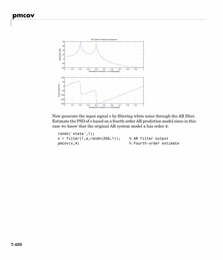
pmcov
Now generate the input signal x by filtering white noise through the AR filter. Estimate the PSD of x based on a fourth-order AR prediction model since in this case we know that the original AR system model a has order 4:
randn('state',1);x = filter(1,a,randn(256,1)); % AR filter outputpmcov(x,4) % Fourth-order estimate
0 0.1 0.2 0.3 0.4 0.5 0.6 0.7 0.8 0.9 1−200
−150
−100
−50
0
50
100
Normalized Frequency (×π rad/sample)
Pha
se (
degr
ees)
0 0.1 0.2 0.3 0.4 0.5 0.6 0.7 0.8 0.9 1−20
−10
0
10
20
30
40
Normalized Frequency (×π rad/sample)
Mag
nitu
de (
dB)
AR System Frequency Response
7-450
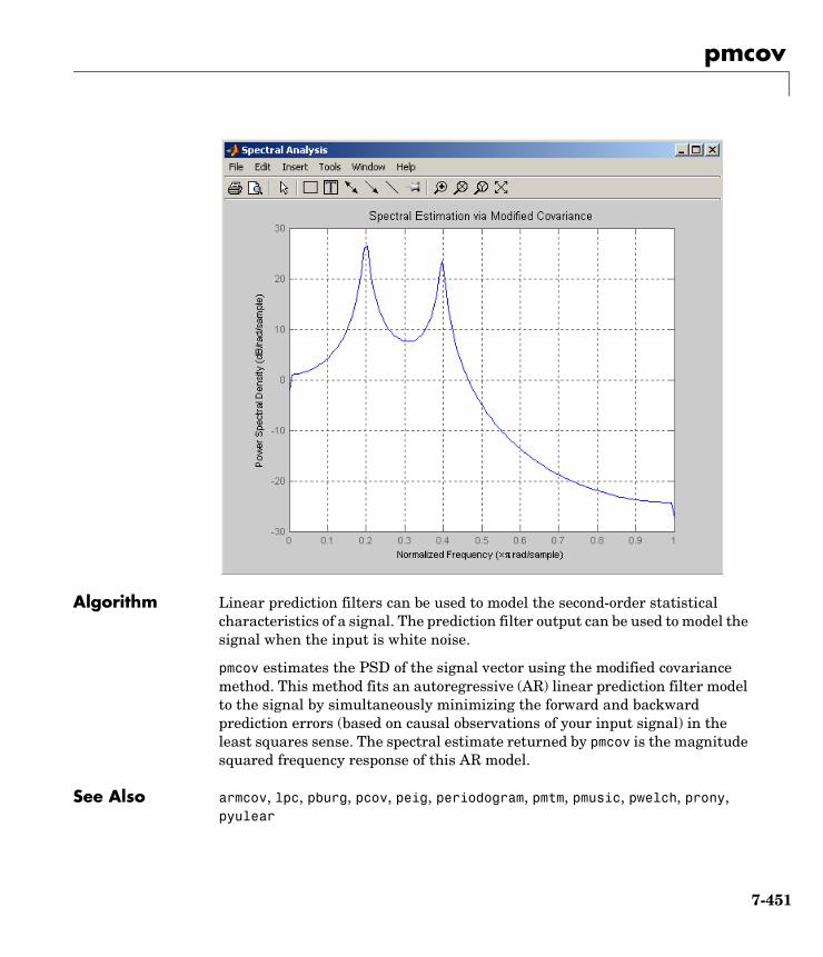
pmcov
Algorithm Linear prediction filters can be used to model the second-order statistical characteristics of a signal. The prediction filter output can be used to model the signal when the input is white noise.
pmcov estimates the PSD of the signal vector using the modified covariance method. This method fits an autoregressive (AR) linear prediction filter model to the signal by simultaneously minimizing the forward and backward prediction errors (based on causal observations of your input signal) in the least squares sense. The spectral estimate returned by pmcov is the magnitude squared frequency response of this AR model.
See Also armcov, lpc, pburg, pcov, peig, periodogram, pmtm, pmusic, pwelch, prony, pyulear
7-451

pmcov
References [1] Marple, S.L. Digital Spectral Analysis, Englewood Cliffs, NJ, Prentice-Hall, 1987, Chapter 7.
[2] Stoica, P., and R.L. Moses, Introduction to Spectral Analysis, Prentice-Hall, 1997.
7-452
pmtm
7pmtmPurpose Estimate the power spectral density using the multitaper method (MTM)
Syntax [Pxx,w] = pmtm(x,nw)[Pxx,w] = pmtm(x,nw,nfft)[Pxx,f] = pmtm(x,nw,nfft,fs)[Pxx,Pxxc,f] = pmtm(x,nw,nfft,fs)[Pxx,Pxxc,f] = pmtm(x,nw,nfft,fs,p)[Pxx,Pxxc,f] = pmtm(x,e,v,nfft,fs,p)[Pxx,Pxxc,f] = pmtm(x,dpss_params,nfft,fs,p)[...] = pmtm(...,'method')[...] = pmtm(...,'range')pmtm(...)
Description pmtm estimates the power spectral density (PSD) of the time series x using the multitaper method (MTM) described in [1]. This method uses linear or nonlinear combinations of modified periodograms to estimate the PSD. These periodograms are computed using a sequence of orthogonal tapers (windows in the frequency domain) specified from the discrete prolate spheroidal sequences (see dpss).
[Pxx,w] = pmtm(x,nw) estimates the PSD Pxx for the input signal x, using 2*nw-1 discrete prolate spheroidal sequences as data tapers for the multitaper estimation method. nw is the time-bandwidth product for the discrete prolate spheroidal sequences. If you specify nw as the empty vector [], a default value of 4 is used. Other typical choices are 2, 5/2, 3, or 7/2. pmtm also returns w, a vector of frequencies at which the PSD is estimated. Pxx and w have the same length. The units for frequency are rad/sample.
The power spectral density is calculated in units of power per radians per sample. Real-valued inputs produce (by default) full power one-sided (in frequency) PSDs, while complex-valued inputs produce two-sided PSDs.
In general, the length N of the FFT and the values of the input x determine the length of Pxx and the range of the corresponding normalized frequencies. For this syntax, the (default) length N of the FFT is the larger of 256 and the next power of two greater than the length of the segment. The following table
7-453
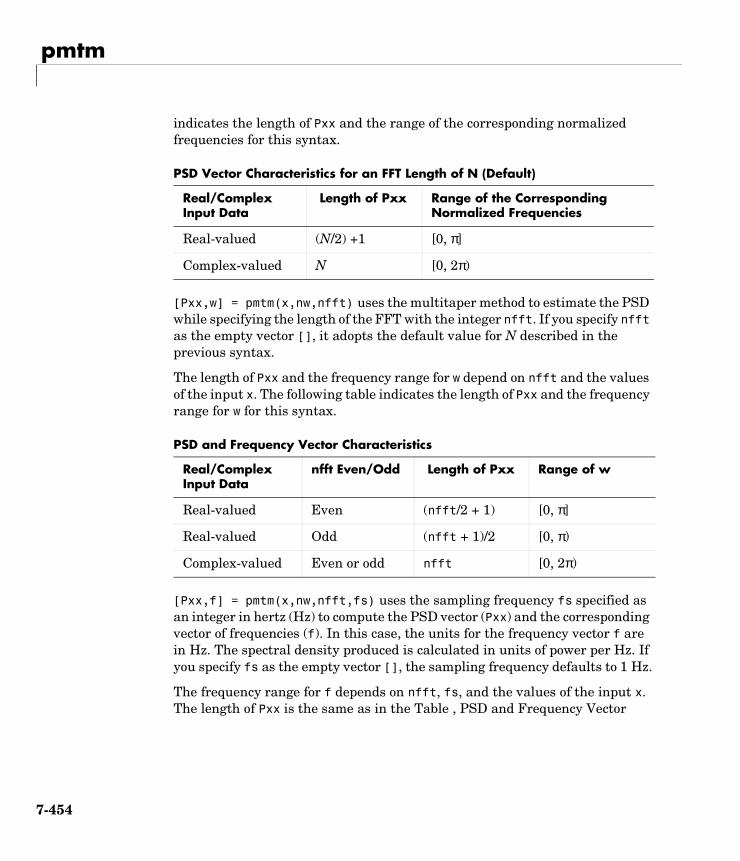
pmtm
indicates the length of Pxx and the range of the corresponding normalized frequencies for this syntax.
[Pxx,w] = pmtm(x,nw,nfft) uses the multitaper method to estimate the PSD while specifying the length of the FFT with the integer nfft. If you specify nfft as the empty vector [], it adopts the default value for N described in the previous syntax.
The length of Pxx and the frequency range for w depend on nfft and the values of the input x. The following table indicates the length of Pxx and the frequency range for w for this syntax.
[Pxx,f] = pmtm(x,nw,nfft,fs) uses the sampling frequency fs specified as an integer in hertz (Hz) to compute the PSD vector (Pxx) and the corresponding vector of frequencies (f). In this case, the units for the frequency vector f are in Hz. The spectral density produced is calculated in units of power per Hz. If you specify fs as the empty vector [], the sampling frequency defaults to 1 Hz.
The frequency range for f depends on nfft, fs, and the values of the input x. The length of Pxx is the same as in the Table , PSD and Frequency Vector
PSD Vector Characteristics for an FFT Length of N (Default)
Real/Complex Input Data
Length of Pxx Range of the Corresponding Normalized Frequencies
Real-valued (N/2) +1 [0, π]
Complex-valued N [0, 2π)
PSD and Frequency Vector Characteristics
Real/Complex Input Data
nfft Even/Odd Length of Pxx Range of w
Real-valued Even (nfft/2 + 1) [0, π]
Real-valued Odd (nfft + 1)/2 [0, π)
Complex-valued Even or odd nfft [0, 2π)
7-454
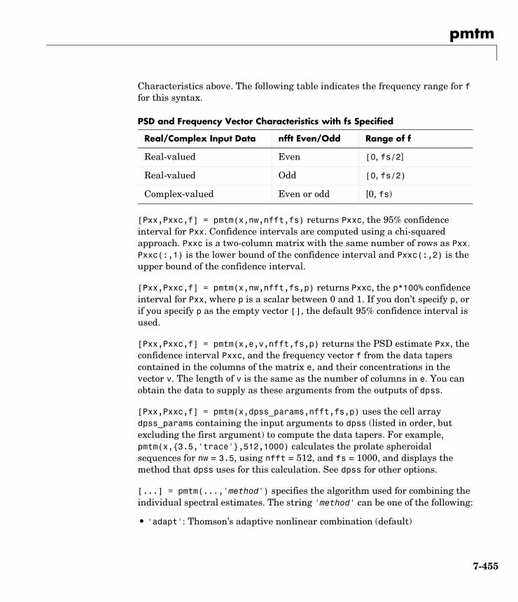
pmtm
Characteristics above. The following table indicates the frequency range for f for this syntax.
[Pxx,Pxxc,f] = pmtm(x,nw,nfft,fs) returns Pxxc, the 95% confidence interval for Pxx. Confidence intervals are computed using a chi-squared approach. Pxxc is a two-column matrix with the same number of rows as Pxx. Pxxc(:,1) is the lower bound of the confidence interval and Pxxc(:,2) is the upper bound of the confidence interval.
[Pxx,Pxxc,f] = pmtm(x,nw,nfft,fs,p) returns Pxxc, the p*100% confidence interval for Pxx, where p is a scalar between 0 and 1. If you don’t specify p, or if you specify p as the empty vector [], the default 95% confidence interval is used.
[Pxx,Pxxc,f] = pmtm(x,e,v,nfft,fs,p) returns the PSD estimate Pxx, the confidence interval Pxxc, and the frequency vector f from the data tapers contained in the columns of the matrix e, and their concentrations in the vector v. The length of v is the same as the number of columns in e. You can obtain the data to supply as these arguments from the outputs of dpss.
[Pxx,Pxxc,f] = pmtm(x,dpss_params,nfft,fs,p) uses the cell array dpss_params containing the input arguments to dpss (listed in order, but excluding the first argument) to compute the data tapers. For example, pmtm(x,3.5,'trace',512,1000) calculates the prolate spheroidal sequences for nw = 3.5, using nfft = 512, and fs = 1000, and displays the method that dpss uses for this calculation. See dpss for other options.
[...] = pmtm(...,'method') specifies the algorithm used for combining the individual spectral estimates. The string 'method' can be one of the following:
• 'adapt': Thomson’s adaptive nonlinear combination (default)
PSD and Frequency Vector Characteristics with fs Specified
Real/Complex Input Data nfft Even/Odd Range of f
Real-valued Even [0, fs/2]
Real-valued Odd [0, fs/2)
Complex-valued Even or odd [0, fs)
7-455
pmtm
• 'unity': A linear combination of the weighted periodograms with unity weights
• 'eigen': A linear combination of the weighted periodograms with eigenvalue weights
[...] = pmtm(...,'range') specifies the range of frequency values to include in f or w. This syntax is useful when x is real. 'range' can be either:
• 'twosided': Compute the two-sided PSD over the frequency range [0,fs). This is the default for determining the frequency range for complex-valued x.
- If you specify fs as the empty vector, [], the frequency range is [0,1).
- If you don’t specify fs, the frequency range is [0, 2π).
• 'onesided': Compute the one-sided PSD over the frequency ranges specified for real x. This is the default for determining the frequency range for real-valued x.
Note You can put the string arguments 'range' or 'method' anywhere after the input argument nw or v.
pmtm(...) with no output arguments plots the PSD estimate and the confidence intervals in the current figure window. If you don’t specify fs, the 95% confidence interval is plotted. If you do specify fs, the confidence intervals plotted depend on the value of p.
7-456
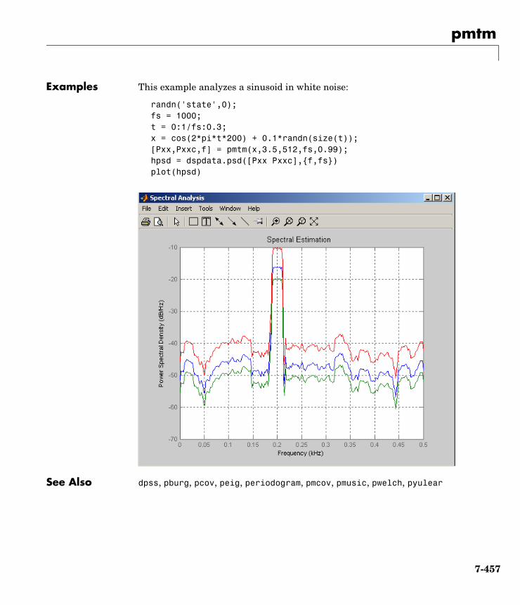
pmtm
Examples This example analyzes a sinusoid in white noise:
randn('state',0);fs = 1000; t = 0:1/fs:0.3;x = cos(2*pi*t*200) + 0.1*randn(size(t));[Pxx,Pxxc,f] = pmtm(x,3.5,512,fs,0.99);hpsd = dspdata.psd([Pxx Pxxc],f,fs)plot(hpsd)
See Also dpss, pburg, pcov, peig, periodogram, pmcov, pmusic, pwelch, pyulear
7-457

pmtm
References [1] Percival, D.B., and A.T. Walden, Spectral Analysis for Physical Applications: Multitaper and Conventional Univariate Techniques, Cambridge University Press, 1993.
[2] Thomson, D.J., “Spectrum estimation and harmonic analysis,” Proceedings of the IEEE, Vol. 70 (1982), pp. 1055-1096.
7-458
pmusic
7pmusicPurpose Estimate the pseudospectrum using the MUSIC algorithm
Syntax [S,w] = pmusic(x,p)[S,w] = pmusic(...,nfft)[S,f] = pmusic(x,p,nfft,fs))[S,f] = pmusic(...,'corr')[S,f] = pmusic(x,p,nfft,fs,nwin,noverlap)[...] = pmusic(...,'range')[...,v,e] = pmusic(...)pmusic(...)
Description [S,w] = pmusic(x,p) implements the MUSIC (Multiple Signal Classification) algorithm and returns S, the pseudospectrum estimate of the input signal x, and a vector w of normalized frequencies (in rad/sample) at which the pseudospectrum is evaluated. The pseudospectrum is calculated using estimates of the eigenvectors of a correlation matrix associated with the input data x, where x is specified as either:
• A row or column vector representing one observation of the signal
• A rectangular array for which each row of x represents a separate observation of the signal (for example, each row is one output of an array of sensors, as in array processing), such that x'*x is an estimate of the correlation matrix
Note You can use the output of corrmtx to generate such an array x.
You can specify the second input argument p as either:
• A scalar integer. In this case, the signal subspace dimension is p.
• A two-element vector. In this case, p(2), the second element of p, represents a threshold that is multiplied by λmin, the smallest estimated eigenvalue of the signal’s correlation matrix. Eigenvalues below the threshold λmin*p(2) are assigned to the noise subspace. In this case, p(1) specifies the maximum dimension of the signal subspace.
7-459
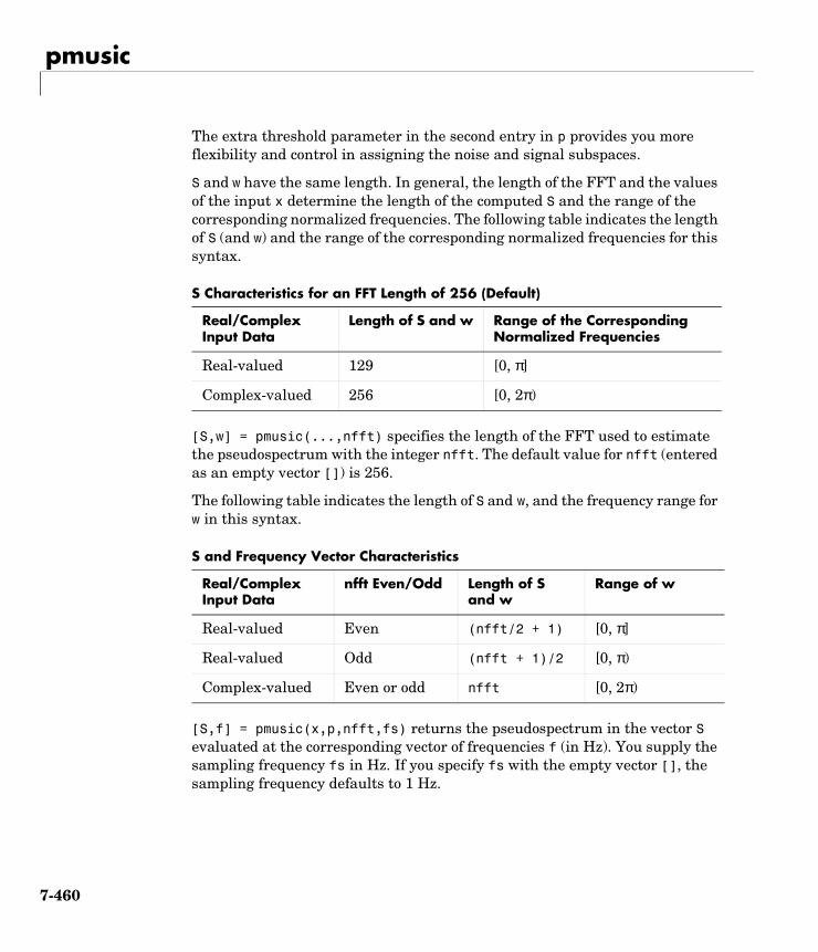
pmusic
The extra threshold parameter in the second entry in p provides you more flexibility and control in assigning the noise and signal subspaces.
S and w have the same length. In general, the length of the FFT and the values of the input x determine the length of the computed S and the range of the corresponding normalized frequencies. The following table indicates the length of S (and w) and the range of the corresponding normalized frequencies for this syntax.
[S,w] = pmusic(...,nfft) specifies the length of the FFT used to estimate the pseudospectrum with the integer nfft. The default value for nfft (entered as an empty vector []) is 256.
The following table indicates the length of S and w, and the frequency range for w in this syntax.
[S,f] = pmusic(x,p,nfft,fs) returns the pseudospectrum in the vector S evaluated at the corresponding vector of frequencies f (in Hz). You supply the sampling frequency fs in Hz. If you specify fs with the empty vector [], the sampling frequency defaults to 1 Hz.
S Characteristics for an FFT Length of 256 (Default)
Real/Complex Input Data
Length of S and w Range of the Corresponding Normalized Frequencies
Real-valued 129 [0, π]
Complex-valued 256 [0, 2π)
S and Frequency Vector Characteristics
Real/Complex Input Data
nfft Even/Odd Length of S and w
Range of w
Real-valued Even (nfft/2 + 1) [0, π]
Real-valued Odd (nfft + 1)/2 [0, π)
Complex-valued Even or odd nfft [0, 2π)
7-460
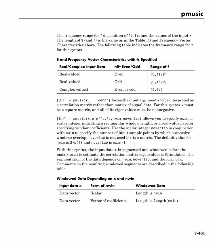
pmusic
The frequency range for f depends on nfft, fs, and the values of the input x. The length of S (and f) is the same as in the Table , S and Frequency Vector Characteristics above. The following table indicates the frequency range for f for this syntax.
[S,f] = pmusic(...,'corr') forces the input argument x to be interpreted as a correlation matrix rather than matrix of signal data. For this syntax x must be a square matrix, and all of its eigenvalues must be nonnegative.
[S,f] = pmusic(x,p,nfft,fs,nwin,noverlap) allows you to specify nwin, a scalar integer indicating a rectangular window length, or a real-valued vector specifying window coefficients. Use the scalar integer noverlap in conjunction with nwin to specify the number of input sample points by which successive windows overlap. noverlap is not used if x is a matrix. The default value for nwin is 2*p(1) and noverlap is nwin-1.
With this syntax, the input data x is segmented and windowed before the matrix used to estimate the correlation matrix eigenvalues is formulated. The segmentation of the data depends on nwin, noverlap, and the form of x. Comments on the resulting windowed segments are described in the following table.
S and Frequency Vector Characteristics with fs Specified
Real/Complex Input Data nfft Even/Odd Range of f
Real-valued Even [0,fs/2]
Real-valued Odd [0,fs/2)
Complex-valued Even or odd [0,fs)
Windowed Data Depending on x and nwin
Input data x Form of nwin Windowed Data
Data vector Scalar Length is nwin
Data vector Vector of coefficients Length is length(nwin)
7-461
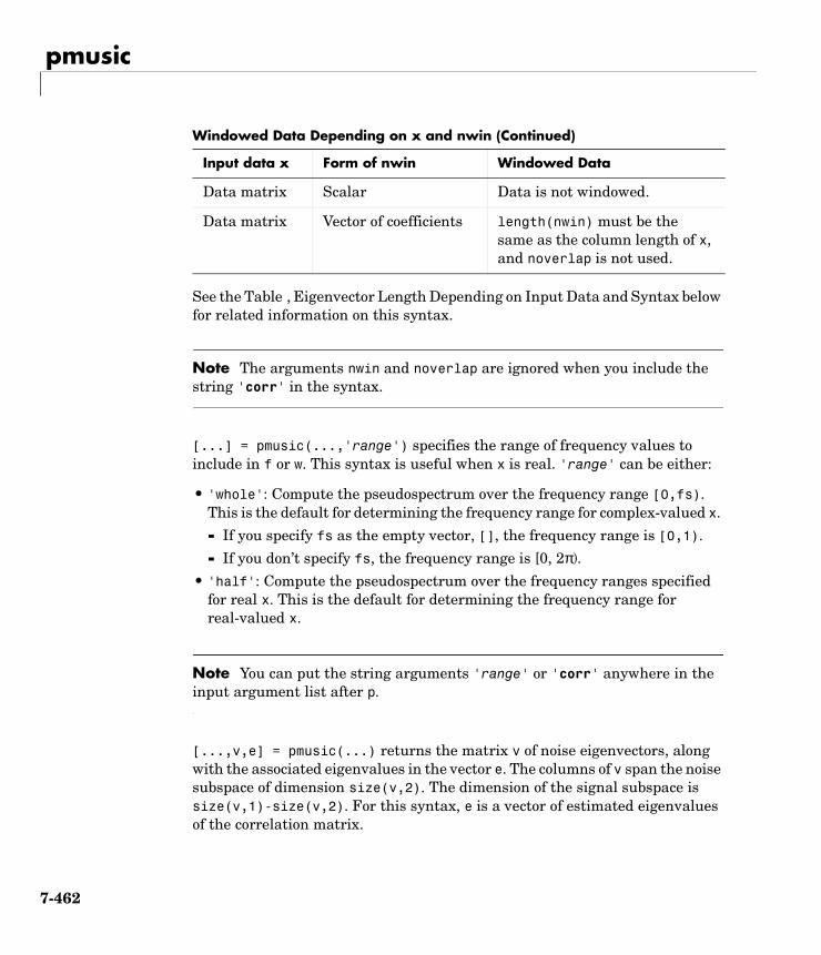
pmusic
See the Table , Eigenvector Length Depending on Input Data and Syntax below for related information on this syntax.
Note The arguments nwin and noverlap are ignored when you include the string 'corr' in the syntax.
[...] = pmusic(...,'range') specifies the range of frequency values to include in f or w. This syntax is useful when x is real. 'range' can be either:
• 'whole': Compute the pseudospectrum over the frequency range [0,fs). This is the default for determining the frequency range for complex-valued x.
- If you specify fs as the empty vector, [], the frequency range is [0,1).
- If you don’t specify fs, the frequency range is [0, 2π).
• 'half': Compute the pseudospectrum over the frequency ranges specified for real x. This is the default for determining the frequency range for real-valued x.
Note You can put the string arguments 'range' or 'corr' anywhere in the input argument list after p.
[...,v,e] = pmusic(...) returns the matrix v of noise eigenvectors, along with the associated eigenvalues in the vector e. The columns of v span the noise subspace of dimension size(v,2). The dimension of the signal subspace is size(v,1)-size(v,2). For this syntax, e is a vector of estimated eigenvalues of the correlation matrix.
Data matrix Scalar Data is not windowed.
Data matrix Vector of coefficients length(nwin) must be the same as the column length of x, and noverlap is not used.
Windowed Data Depending on x and nwin (Continued)
Input data x Form of nwin Windowed Data
7-462
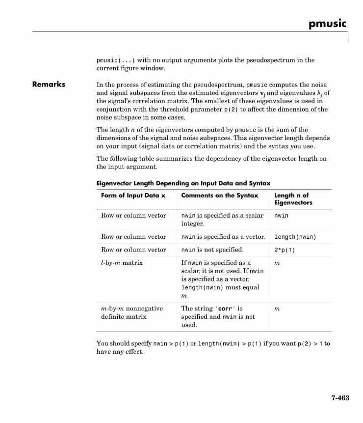
pmusic
pmusic(...) with no output arguments plots the pseudospectrum in the current figure window.
Remarks In the process of estimating the pseudospectrum, pmusic computes the noise and signal subspaces from the estimated eigenvectors vj and eigenvalues λj of the signal’s correlation matrix. The smallest of these eigenvalues is used in conjunction with the threshold parameter p(2) to affect the dimension of the noise subspace in some cases.
The length n of the eigenvectors computed by pmusic is the sum of the dimensions of the signal and noise subspaces. This eigenvector length depends on your input (signal data or correlation matrix) and the syntax you use.
The following table summarizes the dependency of the eigenvector length on the input argument.
You should specify nwin > p(1) or length(nwin) > p(1) if you want p(2) > 1 to have any effect.
Eigenvector Length Depending on Input Data and Syntax
Form of Input Data x Comments on the Syntax Length n of Eigenvectors
Row or column vector nwin is specified as a scalar integer.
nwin
Row or column vector nwin is specified as a vector. length(nwin)
Row or column vector nwin is not specified. 2*p(1)
l-by-m matrix If nwin is specified as a scalar, it is not used. If nwin is specified as a vector, length(nwin) must equal m.
m
m-by-m nonnegative definite matrix
The string 'corr' is specified and nwin is not used.
m
7-463
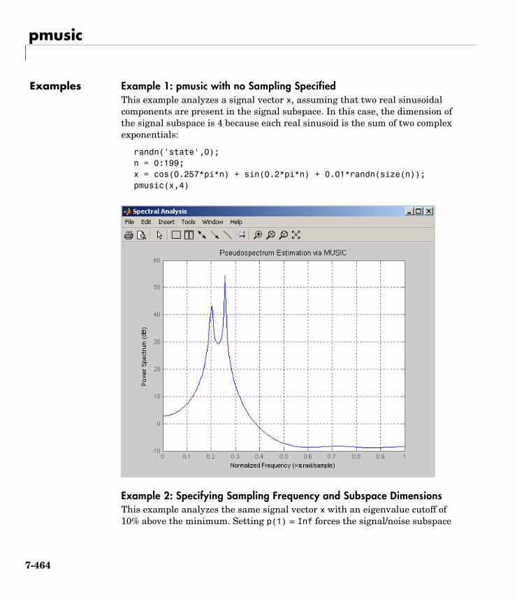
pmusic
Examples Example 1: pmusic with no Sampling SpecifiedThis example analyzes a signal vector x, assuming that two real sinusoidal components are present in the signal subspace. In this case, the dimension of the signal subspace is 4 because each real sinusoid is the sum of two complex exponentials:
randn('state',0);n = 0:199;x = cos(0.257*pi*n) + sin(0.2*pi*n) + 0.01*randn(size(n));pmusic(x,4)
Example 2: Specifying Sampling Frequency and Subspace DimensionsThis example analyzes the same signal vector x with an eigenvalue cutoff of 10% above the minimum. Setting p(1) = Inf forces the signal/noise subspace
7-464
pmusic
decision to be based on the threshold parameter p(2). Specify the eigenvectors of length 7 using the nwin argument, and set the sampling frequency fs to 8 kHz:
randn('state',0);n = 0:199;x = cos(0.257*pi*n) + sin(0.2*pi*n) + 0.01*randn(size(n));[P,f] = pmusic(x,[Inf,1.1],[],8000,7); % Window length = 7
Example 3: Entering a Correlation MatrixSupply a positive definite correlation matrix R for estimating the spectral density. Use the default 256 samples:
R = toeplitz(cos(0.1*pi*[0:6])) + 0.1*eye(7);[P,f] = pmusic(R,4,'corr');
Example 4: Entering a Signal Data Matrix Generated from corrmtxEnter a signal data matrix Xm generated from data using corrmtx:
randn('state',0);n = 0:699;x = cos(0.257*pi*(n)) + 0.1*randn(size(n));Xm = corrmtx(x,7,'mod');[P,w] = pmusic(Xm,2);
Example 5: Using Windowing to Create the Effect of a Signal Data MatrixUse the same signal, but let pmusic form the 100-by-7 data matrix using its windowing input arguments. In addition, specify an FFT of length 512:
randn('state',0);n = 0:699;x = cos(0.257*pi*(n)) + 0.1*randn(size(n));[PP,ff] = pmusic(x,2,512,[],7,0);
Algorithm The name MUSIC is an acronym for MUltiple SIgnal Classification. The MUSIC algorithm estimates the pseudospectrum from a signal or a correlation matrix using Schmidt’s eigenspace analysis method [1]. The algorithm performs eigenspace analysis of the signal’s correlation matrix in order to estimate the signal’s frequency content. This algorithm is particularly suitable for signals that are the sum of sinusoids with additive white Gaussian noise.
7-465
pmusic
The eigenvalues and eigenvectors of the signal’s correlation matrix are estimated if you don’t supply the correlation matrix.
The MUSIC pseudospectrum estimate is given by
where N is the dimension of the eigenvectors and vk is the k-th eigenvector of the correlation matrix. The integer p is the dimension of the signal subspace, so the eigenvectors vk used in the sum correspond to the smallest eigenvalues and also span the noise subspace. The vector e(f) consists of complex exponentials, so the inner product
amounts to a Fourier transform. This is used for computation of the pseudospectrum estimate. The FFT is computed for each vk and then the squared magnitudes are summed.
See Also corrmtx, pburg, peig, periodogram, pmtm, prony, pwelch, rooteig, rootmusic
References [1] Marple, S.L. Digital Spectral Analysis, Englewood Cliffs, NJ, Prentice-Hall, 1987, pp. 373-378.
[2] Schmidt, R.O, “Multiple Emitter Location and Signal Parameter Estimation,” IEEE Trans. Antennas Propagation, Vol. AP-34 (March 1986), pp. 276-280.
[3] Stoica, P., and R.L. Moses, Introduction to Spectral Analysis, Prentice-Hall, Englewood Cliffs, NJ, 1997.
Pmusic f( )1
eH f( ) vkvkH
k p 1+=
N
∑
e f( )
---------------------------------------------------------------- 1
vkHe f( ) 2
k p 1+=
N
∑
-------------------------------------------= =
vkHe f( )
7-466
poly2ac
7poly2acPurpose Convert a prediction filter polynomial to an autocorrelation sequence
Syntax r = poly2ac(a,efinal)
Description r = poly2ac(a,efinal) finds the autocorrelation vector r corresponding to the prediction filter polynomial a. The autocorrelation sequence produced is approximately the same as that of the output of the autoregressive prediction filter whose coefficients are determined by a. poly2ac also produces the final length(r) step prediction error efinal. If a(1) is not equal to 1, poly2ac normalizes the prediction filter polynomial by a(1). a(1) cannot be 0.
Remarks You can apply this function to both real and complex polynomials.
Examples a = [1.0000 0.6147 0.9898 0.0004 0.0034 -0.0077];efinal = 0.2;r = poly2ac(a,efinal)
r = 5.5917 -1.7277 -4.4231 4.3985 1.6426 -5.3126
See Also ac2poly, poly2rc, rc2ac
References [1] Kay, S.M. Modern Spectral Estimation, Englewood Cliffs, NJ, Prentice-Hall, 1988.
7-467
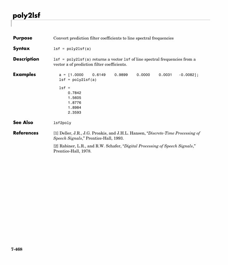
poly2lsf
7poly2lsfPurpose Convert prediction filter coefficients to line spectral frequencies
Syntax lsf = poly2lsf(a)
Description lsf = poly2lsf(a) returns a vector lsf of line spectral frequencies from a vector a of prediction filter coefficients.
Examples a = [1.0000 0.6149 0.9899 0.0000 0.0031 -0.0082];lsf = poly2lsf(a)
lsf = 0.7842 1.5605 1.8776 1.8984 2.3593
See Also lsf2poly
References [1] Deller, J.R., J.G. Proakis, and J.H.L. Hansen, “Discrete-Time Processing of Speech Signals,” Prentice-Hall, 1993.
[2] Rabiner, L.R., and R.W. Schafer, “Digital Processing of Speech Signals,” Prentice-Hall, 1978.
7-468
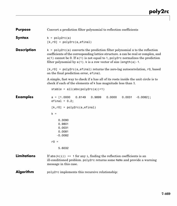
poly2rc
7poly2rcPurpose Convert a prediction filter polynomial to reflection coefficients
Syntax k = poly2rc(a)[k,r0] = poly2rc(a,efinal)
Description k = poly2rc(a) converts the prediction filter polynomial a to the reflection coefficients of the corresponding lattice structure. a can be real or complex, and a(1) cannot be 0. If a(1) is not equal to 1, poly2rc normalizes the prediction filter polynomial by a(1). k is a row vector of size length(a)-1.
[k,r0] = poly2rc(a,efinal) returns the zero-lag autocorrelation, r0, based on the final prediction error, efinal.
A simple, fast way to check if a has all of its roots inside the unit circle is to check if each of the elements of k has magnitude less than 1.
stable = all(abs(poly2rc(a))<1)
Examples a = [1.0000 0.6149 0.9899 0.0000 0.0031 -0.0082];efinal = 0.2;
[k,r0] = poly2rc(a,efinal)
k =
0.3090 0.9801 0.0031 0.0081 -0.0082
r0 =
5.6032
Limitations If abs(k(i)) == 1 for any i, finding the reflection coefficients is an ill-conditioned problem. poly2rc returns some NaNs and provide a warning message in this case.
Algorithm poly2rc implements this recursive relationship:
7-469
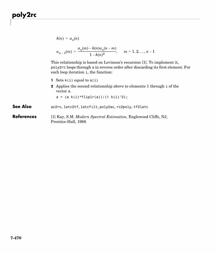
poly2rc
This relationship is based on Levinson’s recursion [1]. To implement it, poly2rc loops through a in reverse order after discarding its first element. For each loop iteration i, the function:
1 Sets k(i) equal to a(i)
2 Applies the second relationship above to elements 1 through i of the vector a.a = (a k(i)*fliplr(a))/(1 k(i)^2);
See Also ac2rc, latc2tf, latcfilt, poly2ac, rc2poly, tf2latc
References [1] Kay, S.M. Modern Spectral Estimation, Englewood Cliffs, NJ, Prentice-Hall, 1988.
k n( ) an n( )=
an 1– m( )an m( ) k n( )an n m–( )–
1 k n( )2–---------------------------------------------------------- m 1= 2 … n 1–, , , ,=
7-470
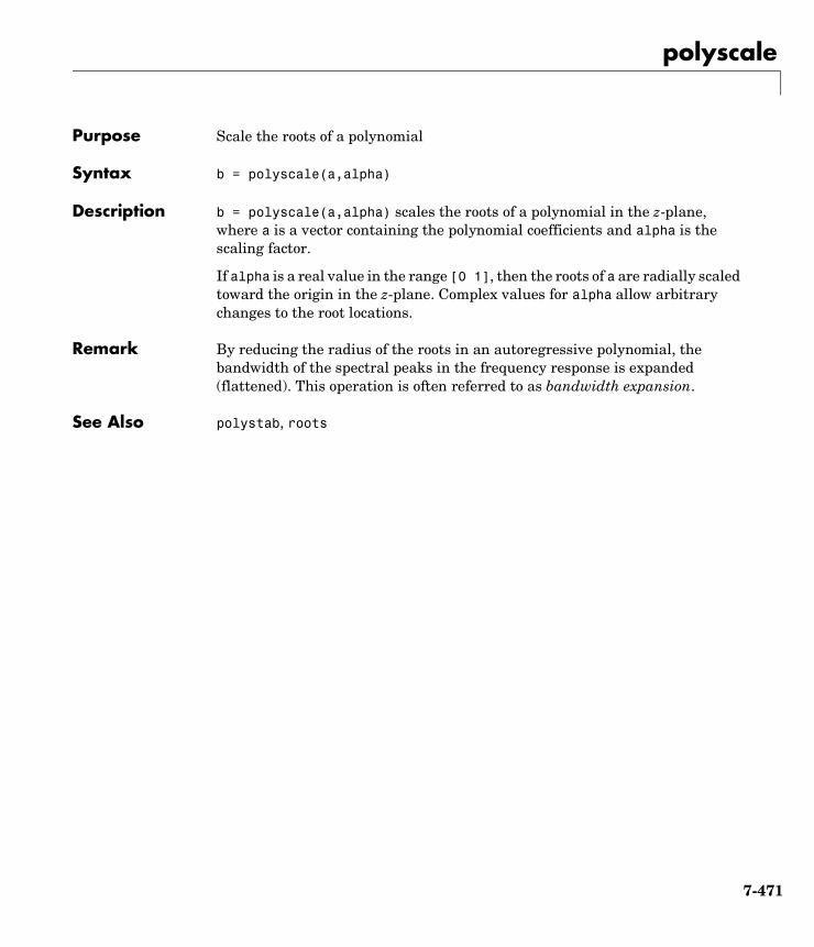
polyscale
7polyscalePurpose Scale the roots of a polynomial
Syntax b = polyscale(a,alpha)
Description b = polyscale(a,alpha) scales the roots of a polynomial in the z-plane, where a is a vector containing the polynomial coefficients and alpha is the scaling factor.
If alpha is a real value in the range [0 1], then the roots of a are radially scaled toward the origin in the z-plane. Complex values for alpha allow arbitrary changes to the root locations.
Remark By reducing the radius of the roots in an autoregressive polynomial, the bandwidth of the spectral peaks in the frequency response is expanded (flattened). This operation is often referred to as bandwidth expansion.
See Also polystab, roots
7-471
polystab
7polystabPurpose Stabilize polynomial
Syntax b = polystab(a)
Description polystab stabilizes a polynomial with respect to the unit circle; it reflects roots with magnitudes greater than 1 inside the unit circle.
b = polystab(a) returns a row vector b containing the stabilized polynomial, where a is a vector of polynomial coefficients, normally in the z-domain.
Examples polystab can convert a linear-phase filter into a minimum-phase filter with the same magnitude response:
h = fir1(25,0.4);hmin = polystab(h) * norm(h)/norm(polystab(h));
Algorithm polystab finds the roots of the polynomial and maps those roots found outside the unit circle to the inside of the unit circle:
v = roots(a);vs = 0.5*(sign(abs(v)-1)+1);v = (1-vs).*v + vs./conj(v);b = a(1)*poly(v);
See Also roots
a z( ) a 1( ) a 2( )z 1– a m 1+( )z m–+ + +=
7-472
prony
7pronyPurpose Prony’s method for time domain IIR filter design
Syntax [b,a] = prony(h,n,m)
Description Prony’s method is an algorithm for finding an IIR filter with a prescribed time domain impulse response. It has applications in filter design, exponential signal modeling, and system identification (parametric modeling).
[b,a] = prony(h,n,m) finds a filter with numerator order n, denominator order m, and the time domain impulse response in h. If the length of h is less than the largest order (n or m), h is padded with zeros. prony returns the filter coefficients in row vectors b and a, of length n + 1 and m + 1, respectively. The filter coefficients are in descending powers of z.
Examples Recover the coefficients of a Butterworth filter from its impulse response:
[b,a] = butter(4,0.2)
b =0.0048 0.0193 0.0289 0.0193 0.0048
a =1.0000 -2.3695 2.3140 -1.0547 0.1874
h = filter(b,a,[1 zeros(1,25)]);[bb,aa] = prony(h,4,4)
bb =0.0048 0.0193 0.0289 0.0193 0.0048
ab =1.0000 -2.3695 2.3140 -1.0547 0.1874
Algorithm prony implements the method described in reference [1]. This method uses a variation of the covariance method of AR modeling to find the denominator coefficients a and then finds the numerator coefficients b for which the impulse
H z( )B z( )A z( )----------- b 1( ) b 2( )z 1– b n 1+( )z n–+ + +
a 1( ) a 2( )z 1– a m 1+( )z m–+ + +----------------------------------------------------------------------------------------= =
7-473

prony
response of the output filter matches exactly the first n + 1 samples of x. The filter is not necessarily stable, but potentially can recover the coefficients exactly if the data sequence is truly an autoregressive moving-average (ARMA) process of the correct order.
See Also butter, cheby1, cheby2, ellip, invfreqz, levinson, lpc, stmcb
References [1] Parks, T.W., and C.S. Burrus, Digital Filter Design, John Wiley & Sons, 1987, pp. 226-228.
7-474
pulstran
7pulstranPurpose Generate a pulse train
Syntax y = pulstran(t,d,'func')y = pulstran(t,d,'func',p1,p2,...)y = pulstran(t,d,p,fs)y = pulstran(t,d,p)
Description pulstran generates pulse trains from continuous functions or sampled prototype pulses.
y = pulstran(t,d,'func') generates a pulse train based on samples of a continuous function, 'func', where 'func' is
• 'gauspuls', for generating a Gaussian-modulated sinusoidal pulse
• 'rectpuls', for generating a sampled aperiodic rectangle
• 'tripuls', for generating a sampled aperiodic triangle
pulstran is evaluated length(d) times and returns the sum of the evaluations y = func(t-d(1)) + func(t-d(2)) + ...
The function is evaluated over the range of argument values specified in array t, after removing a scalar argument offset taken from the vector d. Note that func must be a vectorized function that can take an array t as an argument.
An optional gain factor may be applied to each delayed evaluation by specifying d as a two-column matrix, with the offset defined in column 1 and associated gain in column 2 of d. Note that a row vector will be interpreted as specifying delays only.
pulstran(t,d,'func',p1,p2,...) allows additional parameters to be passed to 'func' as necessary. For example:
func(t-d(1),p1,p2,...) + func(t-d(2),p1,p2,...) + ...
pulstran(t,d,p,fs) generates a pulse train that is the sum of multiple delayed interpolations of the prototype pulse in vector p, sampled at the rate fs, where p spans the time interval [0,(length(p)-1)/fs], and its samples are identically 0 outside this interval. By default, linear interpolation is used for generating delays.
7-475
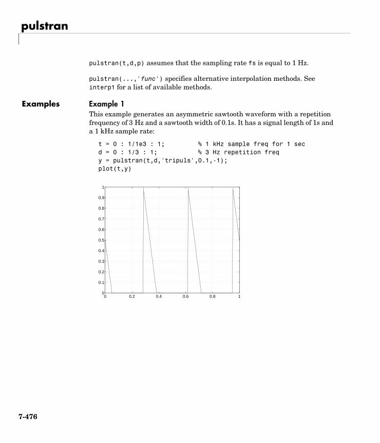
pulstran
pulstran(t,d,p) assumes that the sampling rate fs is equal to 1 Hz.
pulstran(...,'func') specifies alternative interpolation methods. See interp1 for a list of available methods.
Examples Example 1This example generates an asymmetric sawtooth waveform with a repetition frequency of 3 Hz and a sawtooth width of 0.1s. It has a signal length of 1s and a 1 kHz sample rate:
t = 0 : 1/1e3 : 1; % 1 kHz sample freq for 1 sec d = 0 : 1/3 : 1; % 3 Hz repetition freq y = pulstran(t,d,'tripuls',0.1,-1);plot(t,y)
0 0.2 0.4 0.6 0.8 10
0.1
0.2
0.3
0.4
0.5
0.6
0.7
0.8
0.9
1
7-476
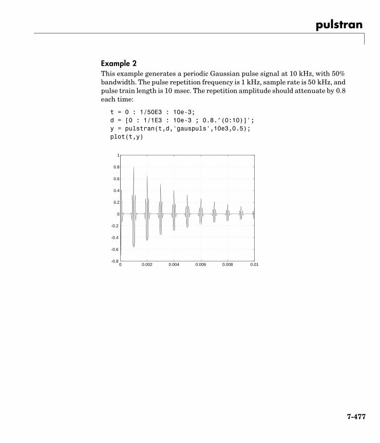
pulstran
Example 2This example generates a periodic Gaussian pulse signal at 10 kHz, with 50% bandwidth. The pulse repetition frequency is 1 kHz, sample rate is 50 kHz, and pulse train length is 10 msec. The repetition amplitude should attenuate by 0.8 each time:
t = 0 : 1/50E3 : 10e-3;d = [0 : 1/1E3 : 10e-3 ; 0.8.^(0:10)]';y = pulstran(t,d,'gauspuls',10e3,0.5); plot(t,y)
0 0.002 0.004 0.006 0.008 0.01-0.8
-0.6
-0.4
-0.2
0
0.2
0.4
0.6
0.8
1
7-477
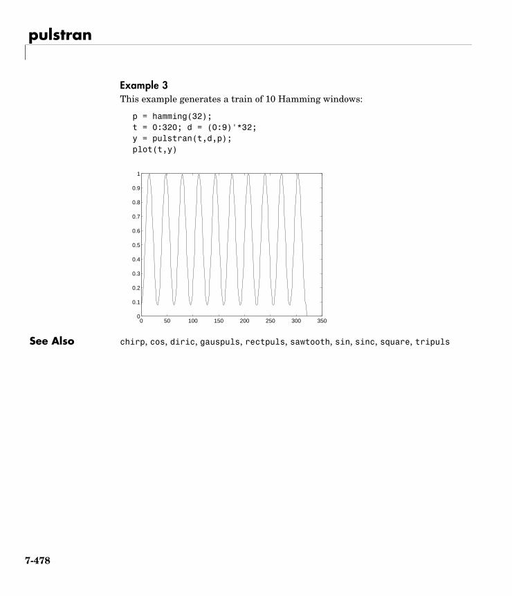
pulstran
Example 3This example generates a train of 10 Hamming windows:
p = hamming(32);t = 0:320; d = (0:9)'*32;y = pulstran(t,d,p);plot(t,y)
See Also chirp, cos, diric, gauspuls, rectpuls, sawtooth, sin, sinc, square, tripuls
0 50 100 150 200 250 300 3500
0.1
0.2
0.3
0.4
0.5
0.6
0.7
0.8
0.9
1
7-478
pwelch
7pwelchPurpose Estimate the power spectral density (PSD) of a signal using Welch’s method
Syntax [Pxx,w] = pwelch(x)[Pxx,w] = pwelch(x,window)[Pxx,w] = pwelch(x,window,noverlap)[Pxx,w] = pwelch(x,window,noverlap,nfft)[Pxx,f] = pwelch(x,window,noverlap,nfft,fs)[...] = pwelch(x,window,noverlap,...,'range')pwelch(...)
Description Note pwelch computes the power spectral density, not the power spectrum. The difference between them is discussed in “Spectral Analysis” on page 3-5.
[Pxx,w] = pwelch(x) estimates the power spectral density Pxx of the input signal vector x using Welch’s averaged modified periodogram method of spectral estimation. With this syntax:
• The vector x is segmented into eight sections of equal length, each with 50% overlap.
• Any remaining (trailing) entries in x that cannot be included in the eight segments of equal length are discarded.
• Each segment is windowed with a Hamming window (see hamming) that is the same length as the segment.
The power spectral density is calculated in units of power per radians per sample. The corresponding vector of frequencies w is computed in radians per sample, and has the same length as Pxx.
A real-valued input vector x produces a full power one-sided (in frequency) PSD (by default), while a complex-valued x produces a two-sided PSD.
In general, the length N of the FFT and the values of the input x determine the length of Pxx and the range of the corresponding normalized frequencies. For this syntax, the (default) length N of the FFT is the larger of 256 and the next power of two greater than the length of the segment. The following table
7-479
pwelch
indicates the length of Pxx and the range of the corresponding normalized frequencies for this syntax.
[Pxx,w] = pwelch(x,window) calculates the modified periodogram using either:
• The window length window for the Hamming window when window is a positive integer
• The window weights specified in window when window is a vector
With this syntax, the input vector x is divided into an integer number of segments with 50% overlap, and each segment is the same length as the window. Entries in x that are left over after it is divided into segments are discarded. If you specify window as the empty vector [], then the signal data is divided into eight segments, and a Hamming window is used on each one.
[Pxx,w] = pwelch(x,window,noverlap) divides x into segments according to window, and uses the integer noverlap to specify the number of signal samples (elements of x) that are common to two adjacent segments. noverlap must be less than the length of the window you specify. If you specify noverlap as the empty vector [], then pwelch determines the segments of x so that there is 50% overlap (default).
[Pxx,w] = pwelch(x,window,noverlap,nfft) uses Welch’s method to estimate the PSD while specifying the length of the FFT with the integer nfft. If you set nfft to the empty vector [], it adopts the default value for N listed in the previous syntax.
PSD Vector Characteristics for an FFT Length of N (Default)
Real/Complex Input Data
Length of Pxx Range of the Corresponding Normalized Frequencies
Real-valued (N/2) +1 [0, π]
Complex-valued N [0, 2π)
7-480
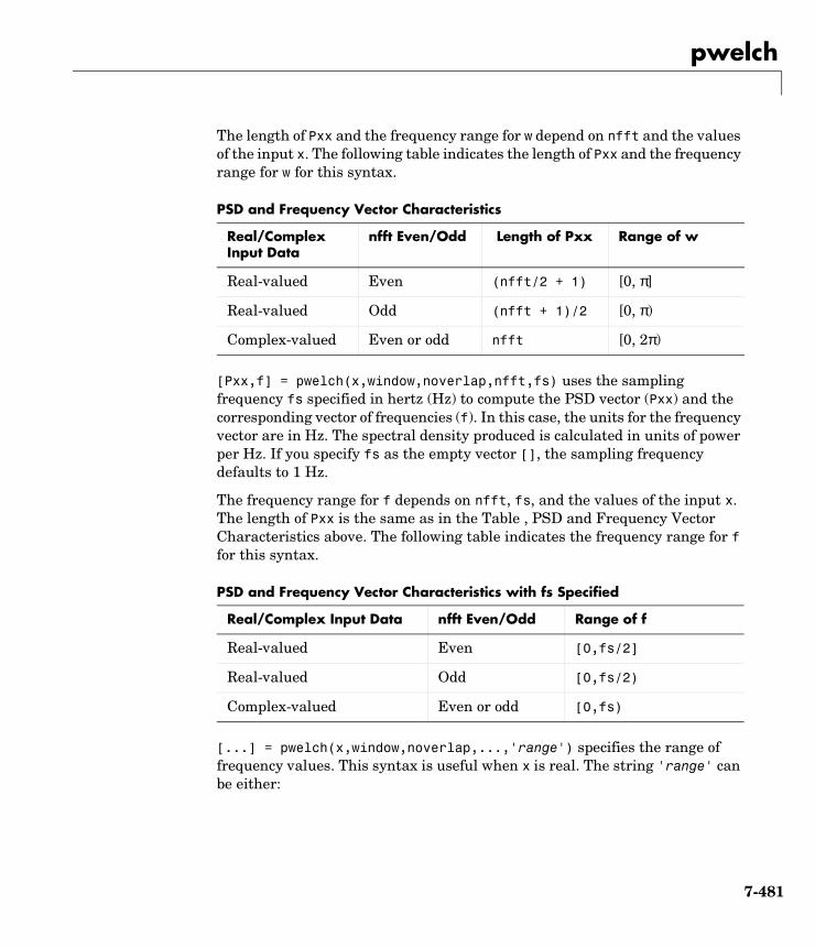
pwelch
The length of Pxx and the frequency range for w depend on nfft and the values of the input x. The following table indicates the length of Pxx and the frequency range for w for this syntax.
[Pxx,f] = pwelch(x,window,noverlap,nfft,fs) uses the sampling frequency fs specified in hertz (Hz) to compute the PSD vector (Pxx) and the corresponding vector of frequencies (f). In this case, the units for the frequency vector are in Hz. The spectral density produced is calculated in units of power per Hz. If you specify fs as the empty vector [], the sampling frequency defaults to 1 Hz.
The frequency range for f depends on nfft, fs, and the values of the input x. The length of Pxx is the same as in the Table , PSD and Frequency Vector Characteristics above. The following table indicates the frequency range for f for this syntax.
[...] = pwelch(x,window,noverlap,...,'range') specifies the range of frequency values. This syntax is useful when x is real. The string 'range' can be either:
PSD and Frequency Vector Characteristics
Real/Complex Input Data
nfft Even/Odd Length of Pxx Range of w
Real-valued Even (nfft/2 + 1) [0, π]
Real-valued Odd (nfft + 1)/2 [0, π)
Complex-valued Even or odd nfft [0, 2π)
PSD and Frequency Vector Characteristics with fs Specified
Real/Complex Input Data nfft Even/Odd Range of f
Real-valued Even [0,fs/2]
Real-valued Odd [0,fs/2)
Complex-valued Even or odd [0,fs)
7-481
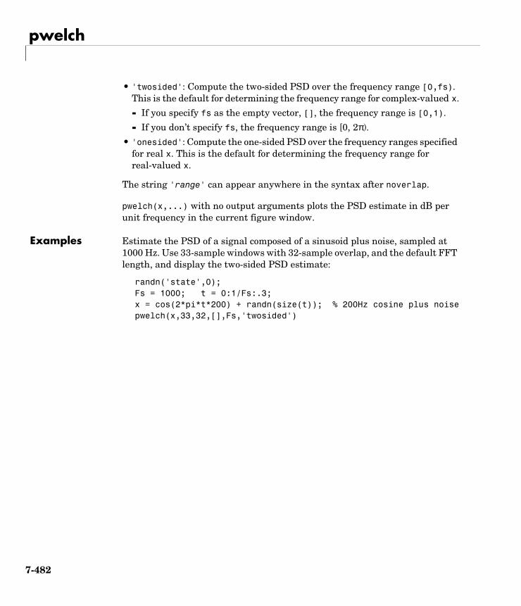
pwelch
• 'twosided': Compute the two-sided PSD over the frequency range [0,fs). This is the default for determining the frequency range for complex-valued x.
- If you specify fs as the empty vector, [], the frequency range is [0,1).
- If you don’t specify fs, the frequency range is [0, 2π).
• 'onesided': Compute the one-sided PSD over the frequency ranges specified for real x. This is the default for determining the frequency range for real-valued x.
The string 'range' can appear anywhere in the syntax after noverlap.
pwelch(x,...) with no output arguments plots the PSD estimate in dB per unit frequency in the current figure window.
Examples Estimate the PSD of a signal composed of a sinusoid plus noise, sampled at 1000 Hz. Use 33-sample windows with 32-sample overlap, and the default FFT length, and display the two-sided PSD estimate:
randn('state',0);Fs = 1000; t = 0:1/Fs:.3;x = cos(2*pi*t*200) + randn(size(t)); % 200Hz cosine plus noisepwelch(x,33,32,[],Fs,'twosided')
7-482
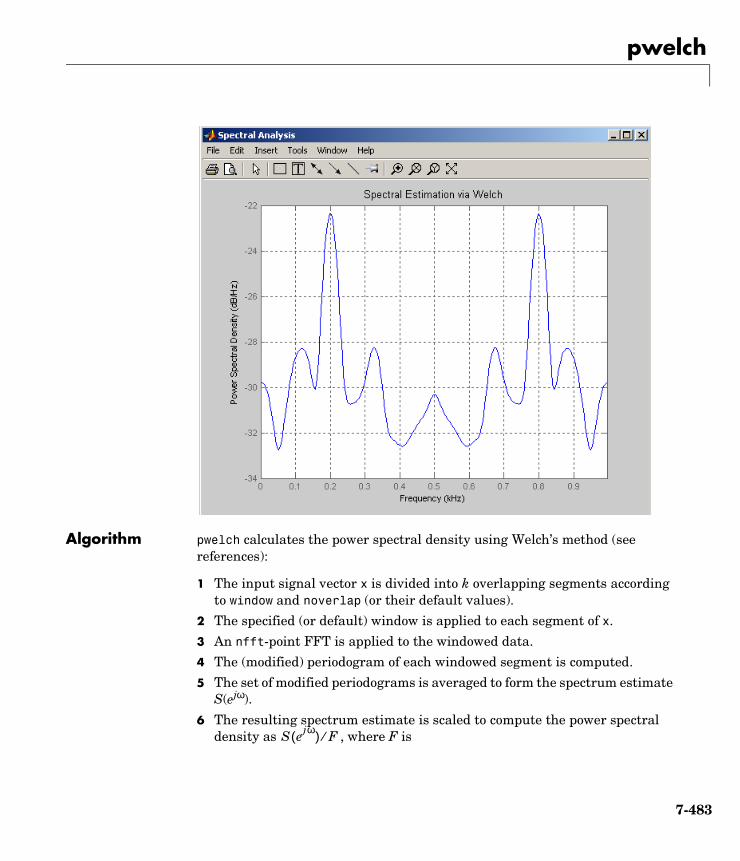
pwelch
Algorithm pwelch calculates the power spectral density using Welch’s method (see references):
1 The input signal vector x is divided into k overlapping segments according to window and noverlap (or their default values).
2 The specified (or default) window is applied to each segment of x.
3 An nfft-point FFT is applied to the windowed data.
4 The (modified) periodogram of each windowed segment is computed.
5 The set of modified periodograms is averaged to form the spectrum estimate S(ejω).
6 The resulting spectrum estimate is scaled to compute the power spectral density as , where F isS ejω( ) F⁄
7-483

pwelch
- 2π when you do not supply the sampling frequency
- fs when you supply the sampling frequency
The number of segments k that x is divided into is calculated as:
• Eight if you don’t specify window, or if you specify it as the empty vector []
• if you specify window as a nonempty vector or a scalar
In this equation, m is the length of the signal vector x, o is the number of overlapping samples (noverlap), and l is the length of each segment (the window length).
See Also dspdata.msspectrum, pburg, pcov, peig, periodogram, pmcov, pmtm, pmusic, pyulear
References [1] Hayes, M., Statistical Digital Signal Processing and Modeling, John Wiley & Sons, 1996.
[2] Stoica, P., and R.L. Moses, Introduction to Spectral Analysis, Prentice-Hall, Englewood Cliffs, NJ, 1997, pp. 52-54.
[3] Welch, P.D, “The Use of Fast Fourier Transform for the Estimation of Power Spectra: A Method Based on Time Averaging Over Short, Modified Periodograms,” IEEE Trans. Audio Electroacoustics, Vol. AU-15 (June 1967), pp. 70-73.
k m o–l o–
--------------=
7-484
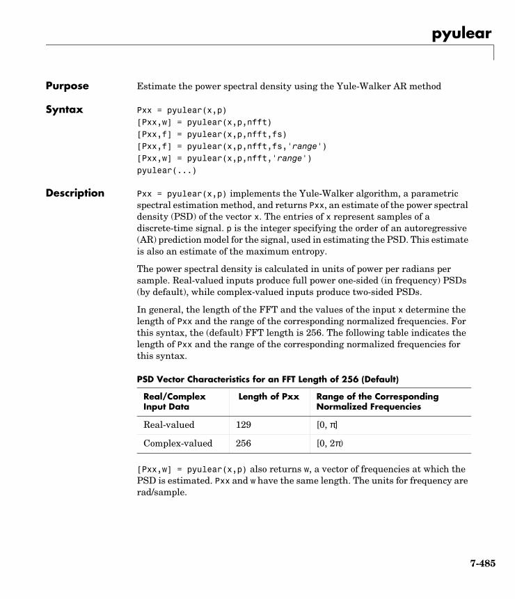
pyulear
7pyulearPurpose Estimate the power spectral density using the Yule-Walker AR method
Syntax Pxx = pyulear(x,p)[Pxx,w] = pyulear(x,p,nfft)[Pxx,f] = pyulear(x,p,nfft,fs)[Pxx,f] = pyulear(x,p,nfft,fs,'range')[Pxx,w] = pyulear(x,p,nfft,'range')pyulear(...)
Description Pxx = pyulear(x,p) implements the Yule-Walker algorithm, a parametric spectral estimation method, and returns Pxx, an estimate of the power spectral density (PSD) of the vector x. The entries of x represent samples of a discrete-time signal. p is the integer specifying the order of an autoregressive (AR) prediction model for the signal, used in estimating the PSD. This estimate is also an estimate of the maximum entropy.
The power spectral density is calculated in units of power per radians per sample. Real-valued inputs produce full power one-sided (in frequency) PSDs (by default), while complex-valued inputs produce two-sided PSDs.
In general, the length of the FFT and the values of the input x determine the length of Pxx and the range of the corresponding normalized frequencies. For this syntax, the (default) FFT length is 256. The following table indicates the length of Pxx and the range of the corresponding normalized frequencies for this syntax.
[Pxx,w] = pyulear(x,p) also returns w, a vector of frequencies at which the PSD is estimated. Pxx and w have the same length. The units for frequency are rad/sample.
PSD Vector Characteristics for an FFT Length of 256 (Default)
Real/Complex Input Data
Length of Pxx Range of the Corresponding Normalized Frequencies
Real-valued 129 [0, π]
Complex-valued 256 [0, 2π)
7-485
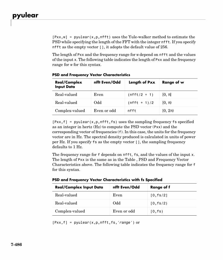
pyulear
[Pxx,w] = pyulear(x,p,nfft) uses the Yule-walker method to estimate the PSD while specifying the length of the FFT with the integer nfft. If you specify nfft as the empty vector [], it adopts the default value of 256.
The length of Pxx and the frequency range for w depend on nfft and the values of the input x. The following table indicates the length of Pxx and the frequency range for w for this syntax.
[Pxx,f] = pyulear(x,p,nfft,fs) uses the sampling frequency fs specified as an integer in hertz (Hz) to compute the PSD vector (Pxx) and the corresponding vector of frequencies (f). In this case, the units for the frequency vector are in Hz. The spectral density produced is calculated in units of power per Hz. If you specify fs as the empty vector [], the sampling frequency defaults to 1 Hz.
The frequency range for f depends on nfft, fs, and the values of the input x. The length of Pxx is the same as in the Table , PSD and Frequency Vector Characteristics above. The following table indicates the frequency range for f for this syntax.
[Pxx,f] = pyulear(x,p,nfft,fs,'range') or
PSD and Frequency Vector Characteristics
Real/Complex Input Data
nfft Even/Odd Length of Pxx Range of w
Real-valued Even (nfft/2 + 1) [0, π]
Real-valued Odd (nfft + 1)/2 [0, π)
Complex-valued Even or odd nfft [0, 2π)
PSD and Frequency Vector Characteristics with fs Specified
Real/Complex Input Data nfft Even/Odd Range of f
Real-valued Even [0,fs/2]
Real-valued Odd [0,fs/2)
Complex-valued Even or odd [0,fs)
7-486
pyulear
[Pxx,w] = pyulear(x,p,nfft,'range') specifies the range of frequency values to include in f or w. This syntax is useful when x is real. 'range' can be either:
• 'twosided': Compute the two-sided PSD over the frequency range [0,fs). This is the default for determining the frequency range for complex-valued x.
- If you specify fs as the empty vector, [], the frequency range is [0,1).
- If you don’t specify fs, the frequency range is [0, 2π).
• 'onesided': Compute the one-sided PSD over the frequency ranges specified for real x. This is the default for determining the frequency range for real-valued x.
Note You can put the string argument 'range' anywhere in the input argument list after p.
pyulear(...) plots the power spectral density in the current figure window. The frequency range on the plot is the same as the range of output w (or f) for a given set of parameters.
Remarks The power spectral density is computed as the distribution of power per unit frequency.
This algorithm depends on your selecting an appropriate model order for your signal.
Examples Because the Yule-walker method estimates the spectral density by fitting an AR prediction model of a given order to the signal, first generate a signal from an AR (all-pole) model of a given order. You can use freqz to check the magnitude of the frequency response of your AR filter. This will give you an idea of what to expect when you estimate the PSD using pyulear:
a = [1 -2.2137 2.9403 -2.1697 0.9606]; % AR filter coefficientsfreqz(1,a) % AR filter frequency responsetitle('AR System Frequency Response')
7-487

pyulear
Now generate the input signal x by filtering white noise through the AR filter. Estimate the PSD of x based on a fourth-order AR prediction model, since in this case, we know that the original AR system model a has order 4:
randn('state',1);x = filter(1,a,randn(256,1)); % AR system outputpyulear(x,4) % Fourth-order estimate
0 0.1 0.2 0.3 0.4 0.5 0.6 0.7 0.8 0.9 1−200
−150
−100
−50
0
50
100
Normalized Frequency (×π rad/sample)
Pha
se (
degr
ees)
0 0.1 0.2 0.3 0.4 0.5 0.6 0.7 0.8 0.9 1−20
−10
0
10
20
30
40
Normalized Frequency (×π rad/sample)
Mag
nitu
de (
dB)
AR System Frequency Response
7-488
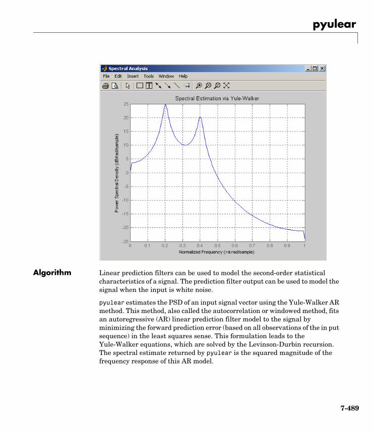
pyulear
Algorithm Linear prediction filters can be used to model the second-order statistical characteristics of a signal. The prediction filter output can be used to model the signal when the input is white noise.
pyulear estimates the PSD of an input signal vector using the Yule-Walker AR method. This method, also called the autocorrelation or windowed method, fits an autoregressive (AR) linear prediction filter model to the signal by minimizing the forward prediction error (based on all observations of the in put sequence) in the least squares sense. This formulation leads to the Yule-Walker equations, which are solved by the Levinson-Durbin recursion. The spectral estimate returned by pyulear is the squared magnitude of the frequency response of this AR model.
7-489

pyulear
See Also aryule, lpc, pburg, pcov, peig, periodogram, pmcov, pmtm, pmusic, prony, pwelch
References [1] Marple, S.L., Digital Spectral Analysis, Prentice-Hall, 1987, Chapter 7.
[2] Stoica, P., and R.L. Moses, Introduction to Spectral Analysis, Prentice-Hall, 1997.
7-490

pyulear
7-491
rc2ac
7rc2acPurpose Convert reflection coefficients to an autocorrelation sequence
Syntax r = rc2ac(k,r0)
Description r = rc2ac(k,r0) finds the autocorrelation coefficients, r, of the output of the discrete-time prediction error filter from the lattice-form reflection coefficients k and initial zero-lag autocorrelation r0.
Examples k = [0.3090 0.9800 0.0031 0.0082 -0.0082];r0 = 0.1;a = rc2ac(k,r0)
a = 0.1000 -0.0309 -0.0791 0.0787 0.0294 -0.0950
See Also ac2rc, poly2ac, rc2poly
References [1] Kay, S.M., Modern Spectral Estimation, Prentice-Hall, Englewood Cliffs, NJ, 1988.
7-492
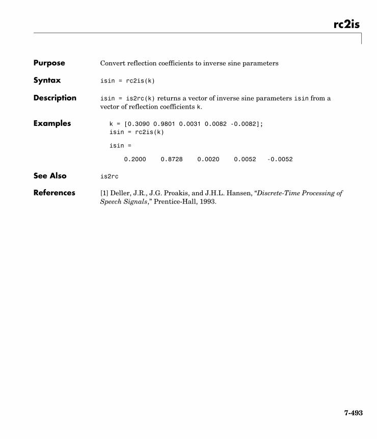
rc2is
7rc2isPurpose Convert reflection coefficients to inverse sine parameters
Syntax isin = rc2is(k)
Description isin = is2rc(k) returns a vector of inverse sine parameters isin from a vector of reflection coefficients k.
Examples k = [0.3090 0.9801 0.0031 0.0082 -0.0082];isin = rc2is(k)
isin =
0.2000 0.8728 0.0020 0.0052 -0.0052
See Also is2rc
References [1] Deller, J.R., J.G. Proakis, and J.H.L. Hansen, “Discrete-Time Processing of Speech Signals,” Prentice-Hall, 1993.
7-493
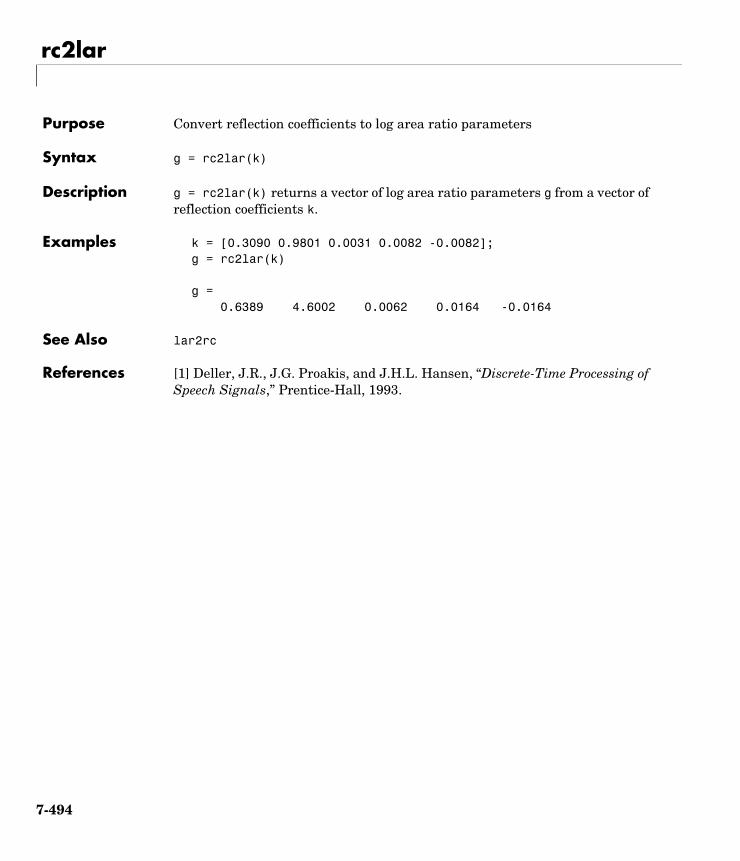
rc2lar
7rc2larPurpose Convert reflection coefficients to log area ratio parameters
Syntax g = rc2lar(k)
Description g = rc2lar(k) returns a vector of log area ratio parameters g from a vector of reflection coefficients k.
Examples k = [0.3090 0.9801 0.0031 0.0082 -0.0082];g = rc2lar(k)
g = 0.6389 4.6002 0.0062 0.0164 -0.0164
See Also lar2rc
References [1] Deller, J.R., J.G. Proakis, and J.H.L. Hansen, “Discrete-Time Processing of Speech Signals,” Prentice-Hall, 1993.
7-494
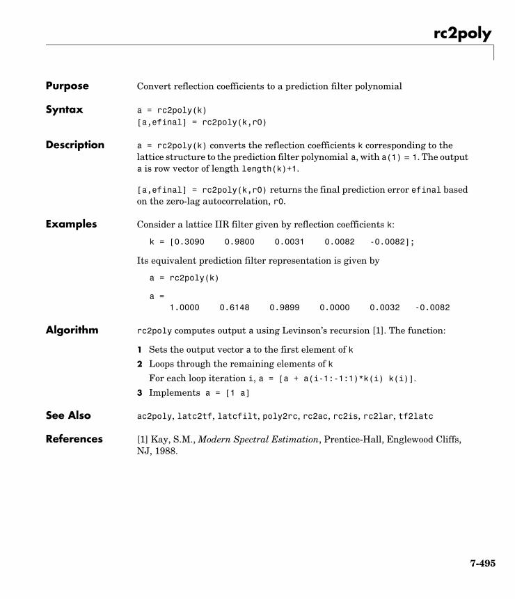
rc2poly
7rc2polyPurpose Convert reflection coefficients to a prediction filter polynomial
Syntax a = rc2poly(k)[a,efinal] = rc2poly(k,r0)
Description a = rc2poly(k) converts the reflection coefficients k corresponding to the lattice structure to the prediction filter polynomial a, with a(1) = 1. The output a is row vector of length length(k)+1.
[a,efinal] = rc2poly(k,r0) returns the final prediction error efinal based on the zero-lag autocorrelation, r0.
Examples Consider a lattice IIR filter given by reflection coefficients k:
k = [0.3090 0.9800 0.0031 0.0082 -0.0082];
Its equivalent prediction filter representation is given by
a = rc2poly(k)
a = 1.0000 0.6148 0.9899 0.0000 0.0032 -0.0082
Algorithm rc2poly computes output a using Levinson’s recursion [1]. The function:
1 Sets the output vector a to the first element of k
2 Loops through the remaining elements of k
For each loop iteration i, a = [a + a(i-1:-1:1)*k(i) k(i)].
3 Implements a = [1 a]
See Also ac2poly, latc2tf, latcfilt, poly2rc, rc2ac, rc2is, rc2lar, tf2latc
References [1] Kay, S.M., Modern Spectral Estimation, Prentice-Hall, Englewood Cliffs, NJ, 1988.
7-495
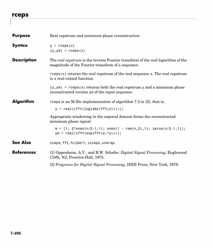
rceps
7rcepsPurpose Real cepstrum and minimum phase reconstruction
Syntax y = rceps(x)[y,ym] = rceps(x)
Description The real cepstrum is the inverse Fourier transform of the real logarithm of the magnitude of the Fourier transform of a sequence.
rceps(x) returns the real cepstrum of the real sequence x. The real cepstrum is a real-valued function.
[y,ym] = rceps(x) returns both the real cepstrum y and a minimum phase reconstructed version ym of the input sequence.
Algorithm rceps is an M-file implementation of algorithm 7.2 in [2], that is,
y = real(ifft(log(abs(fft(x)))));
Appropriate windowing in the cepstral domain forms the reconstructed minimum phase signal:
w = [1; 2*ones(n/2-1,1); ones(1 - rem(n,2),1); zeros(n/2-1,1)];ym = real(ifft(exp(fft(w.*y))));
See Also cceps, fft, hilbert, icceps, unwrap
References [1] Oppenheim, A.V., and R.W. Schafer, Digital Signal Processing, Englewood Cliffs, NJ, Prentice-Hall, 1975.
[2] Programs for Digital Signal Processing, IEEE Press, New York, 1979.
7-496
rectpuls
7rectpulsPurpose Generate a sampled aperiodic rectangle
Syntax y = rectpuls(t)y = rectpuls(t,w)
Description y = rectpuls(t) returns a continuous, aperiodic, unity-height rectangular pulse at the sample times indicated in array t, centered about t = 0 and with a default width of 1. Note that the interval of non-zero amplitude is defined to be open on the right, that is, rectpuls(-0.5) = 1 while rectpuls(0.5) = 0.
y = rectpuls(t,w) generates a rectangle of width w.
rectpuls is typically used in conjunction with the pulse train generating function pulstran.
See Also chirp, cos, diric, gauspuls, pulstran, sawtooth, sin, sinc, square, tripuls
7-497

rectwin
7rectwinPurpose Compute a rectangular window
Syntax w = rectwin(n)
Description w = rectwin(n) returns a rectangular window of length n in the column vector w. This function is provided for completeness; a rectangular window is equivalent to no window at all.
Algorithm w = ones(n,1);
See Also barthannwin, bartlett, blackmanharris, bohmanwin, nuttallwin, parzenwin, triang, window, wintool, wvtool
References [1] Oppenheim, A.V., and R.W. Schafer. Discrete-Time Signal Processing. Upper Saddle River, NJ: Prentice-Hall, 1999, pp. 468-471.
7-498
resample
7resamplePurpose Change sampling rate by any rational factor
Syntax y = resample(x,p,q)y = resample(x,p,q,n)y = resample(x,p,q,n,beta)y = resample(x,p,q,b)[y,b] = resample(x,p,q)
Description y = resample(x,p,q) resamples the sequence in vector x at p/q times the original sampling rate, using a polyphase filter implementation. p and q must be positive integers. The length of y is equal to ceil(length(x)*p/q). If x is a matrix, resample works down the columns of x.
resample applies an anti-aliasing (lowpass) FIR filter to x during the resampling process. It designs the filter using firls with a Kaiser window.
y = resample(x,p,q,n) uses n terms on either side of the current sample, x(k), to perform the resampling. The length of the FIR filter resample uses is proportional to n; larger values of n provide better accuracy at the expense of more computation time. The default for n is 10. If you let n = 0, resample performs a nearest-neighbor interpolation
y(k) = x(round((k-1)*q/p)+1)
where y(k) = 0 if the index to x is greater than length(x).
y = resample(x,p,q,n,beta) uses beta as the design parameter for the Kaiser window that resample employs in designing the lowpass filter. The default for beta is 5.
y = resample(x,p,q,b) filters x using the vector of filter coefficients b.
[y,b] = resample(x,p,q) returns the vector b, which contains the coefficients of the filter applied to x during the resampling process.
Examples Resample a simple linear sequence at 3/2 the original rate:
fs1 = 10; % Original sampling frequency in Hzt1 = 0:1/fs1:1; % Time vectorx = t1; % Define a linear sequencey = resample(x,3,2); % Now resample it
7-499
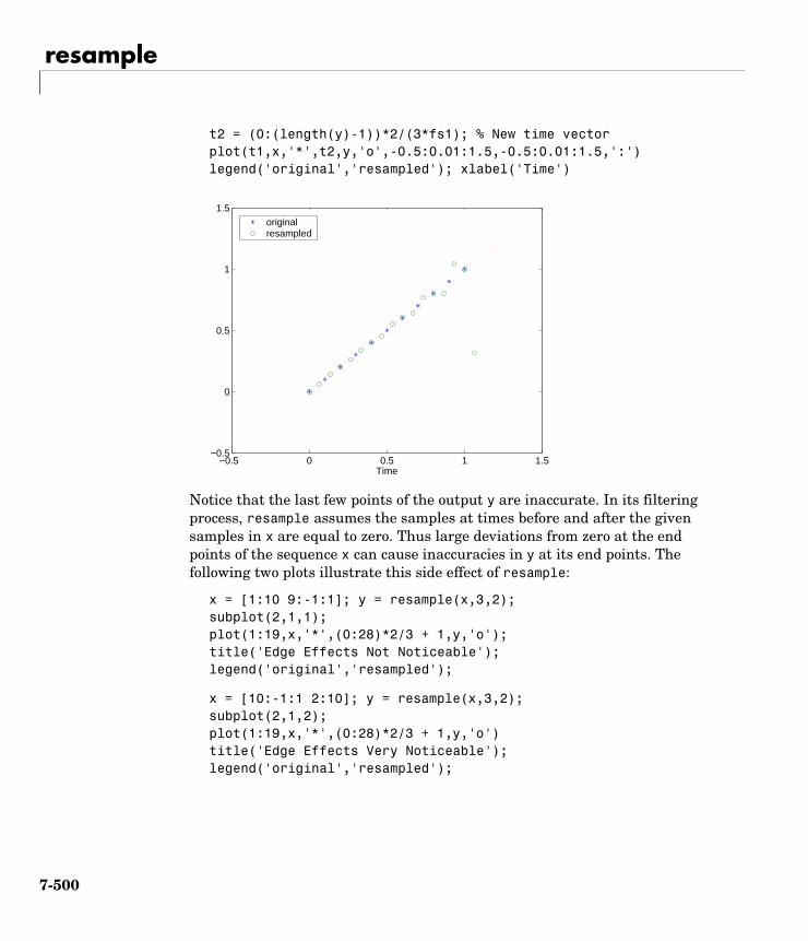
resample
t2 = (0:(length(y)-1))*2/(3*fs1); % New time vectorplot(t1,x,'*',t2,y,'o',-0.5:0.01:1.5,-0.5:0.01:1.5,':')legend('original','resampled'); xlabel('Time')
Notice that the last few points of the output y are inaccurate. In its filtering process, resample assumes the samples at times before and after the given samples in x are equal to zero. Thus large deviations from zero at the end points of the sequence x can cause inaccuracies in y at its end points. The following two plots illustrate this side effect of resample:
x = [1:10 9:-1:1]; y = resample(x,3,2);subplot(2,1,1);plot(1:19,x,'*',(0:28)*2/3 + 1,y,'o');title('Edge Effects Not Noticeable');legend('original','resampled');
x = [10:-1:1 2:10]; y = resample(x,3,2);subplot(2,1,2);plot(1:19,x,'*',(0:28)*2/3 + 1,y,'o')title('Edge Effects Very Noticeable');legend('original','resampled');
−0.5 0 0.5 1 1.5−0.5
0
0.5
1
1.5
Time
original resampled
7-500
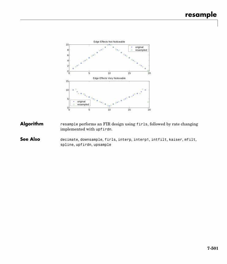
resample
Algorithm resample performs an FIR design using firls, followed by rate changing implemented with upfirdn.
See Also decimate, downsample, firls, interp, interp1, intfilt, kaiser, mfilt, spline, upfirdn, upsample
0 5 10 15 200
2
4
6
8
10Edge Effects Not Noticeable
original resampled
0 5 10 15 200
5
10
15Edge Effects Very Noticeable
original resampled
7-501
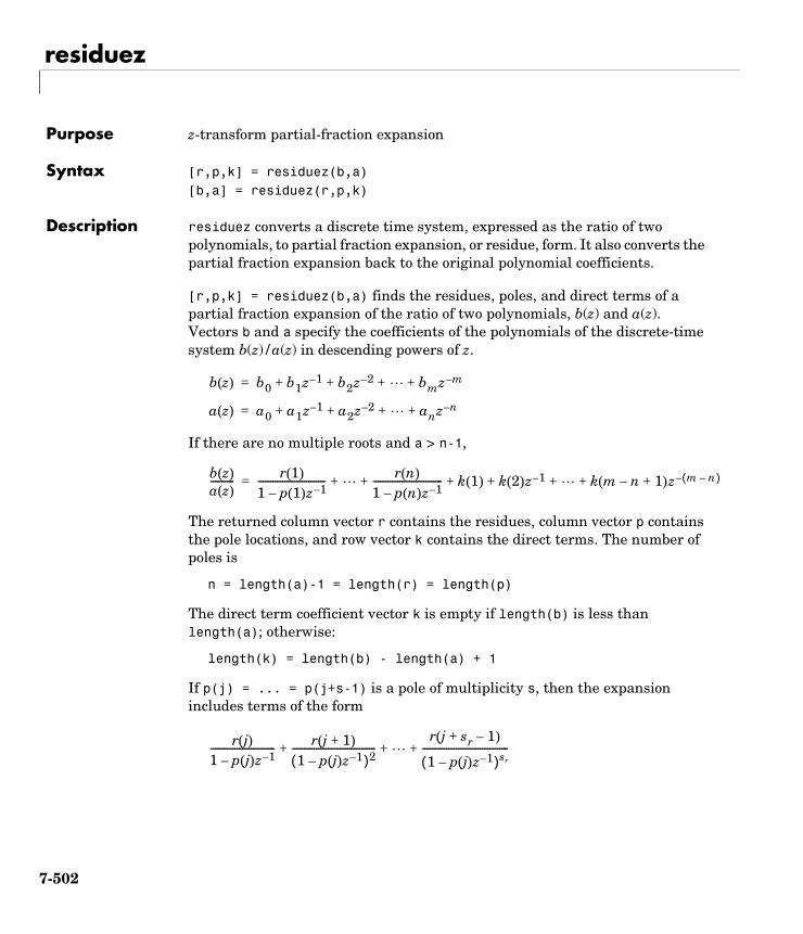
residuez
7residuezPurpose z-transform partial-fraction expansion
Syntax [r,p,k] = residuez(b,a)[b,a] = residuez(r,p,k)
Description residuez converts a discrete time system, expressed as the ratio of two polynomials, to partial fraction expansion, or residue, form. It also converts the partial fraction expansion back to the original polynomial coefficients.
[r,p,k] = residuez(b,a) finds the residues, poles, and direct terms of a partial fraction expansion of the ratio of two polynomials, b(z) and a(z). Vectors b and a specify the coefficients of the polynomials of the discrete-time system b(z)/a(z) in descending powers of z.
If there are no multiple roots and a > n-1,
The returned column vector r contains the residues, column vector p contains the pole locations, and row vector k contains the direct terms. The number of poles is
n = length(a)-1 = length(r) = length(p)
The direct term coefficient vector k is empty if length(b) is less than length(a); otherwise:
length(k) = length(b) - length(a) + 1
If p(j) = ... = p(j+s-1) is a pole of multiplicity s, then the expansion includes terms of the form
b z( ) b0 b1z 1– b2z 2– bmz m–+ + + +=
a z( ) a0 a1z 1– a2z 2– anz n–+ + + +=
b z( )a z( )---------- r 1( )
1 p 1( )z 1––---------------------------- r n( )
1 p n( )z 1––----------------------------- k 1( ) k 2( )z 1– k m n 1+–( )z m n–( )–+ + + + + +=
r j( )1 p j( )z 1––--------------------------- r j 1+( )
1 p j( )z 1––( )2-----------------------------------
r j sr 1–+( )
1 p j( )z 1––( )sr------------------------------------+ + +
7-502
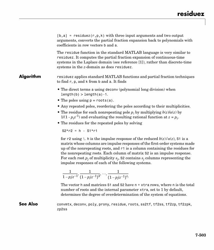
residuez
[b,a] = residuez(r,p,k) with three input arguments and two output arguments, converts the partial fraction expansion back to polynomials with coefficients in row vectors b and a.
The residue function in the standard MATLAB language is very similar to residuez. It computes the partial fraction expansion of continuous-time systems in the Laplace domain (see reference [1]), rather than discrete-time systems in the z-domain as does residuez.
Algorithm residuez applies standard MATLAB functions and partial fraction techniques to find r, p, and k from b and a. It finds
• The direct terms a using deconv (polynomial long division) when length(b) > length(a)-1.
• The poles using p = roots(a).
• Any repeated poles, reordering the poles according to their multiplicities.
• The residue for each nonrepeating pole pi by multiplying b(z)/a(z) by 1/(1 - piz
-1) and evaluating the resulting rational function at z = pi.
• The residues for the repeated poles by solving
S2*r2 = h - S1*r1
for r2 using \. h is the impulse response of the reduced b(z)/a(z), S1 is a matrix whose columns are impulse responses of the first-order systems made up of the nonrepeating roots, and r1 is a column containing the residues for the nonrepeating roots. Each column of matrix S2 is an impulse response. For each root pj of multiplicity sj, S2 contains sj columns representing the impulse responses of each of the following systems.
The vector h and matrices S1 and S2 have n + xtra rows, where n is the total number of roots and the internal parameter xtra, set to 1 by default, determines the degree of overdetermination of the system of equations.
See Also convmtx, deconv, poly, prony, residue, roots, ss2tf, tf2ss, tf2zp, tf2zpk, zp2ss
11 pjz 1––----------------------- 1
1 pjz 1––( )2------------------------------- 1
1 pjz 1––( )sj--------------------------------, , ,
7-503

residuez
References [1] Oppenheim, A.V., and R.W. Schafer, Digital Signal Processing, Prentice-Hall, Englewood Cliffs, NJ, 1975, pp. 166-170.
7-504
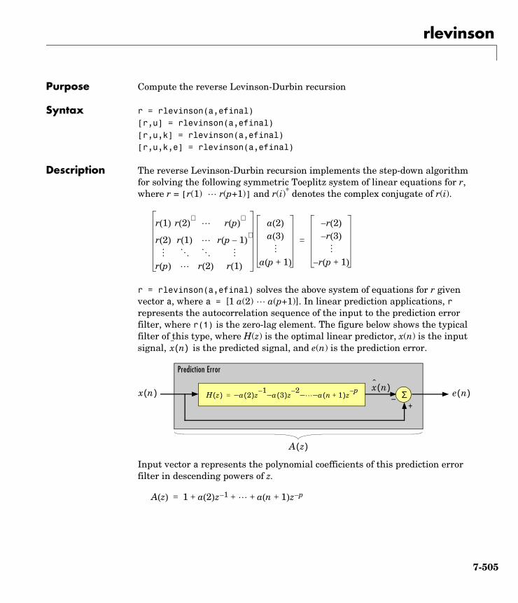
rlevinson
7rlevinsonPurpose Compute the reverse Levinson-Durbin recursion
Syntax r = rlevinson(a,efinal)[r,u] = rlevinson(a,efinal)[r,u,k] = rlevinson(a,efinal)[r,u,k,e] = rlevinson(a,efinal)
Description The reverse Levinson-Durbin recursion implements the step-down algorithm for solving the following symmetric Toeplitz system of linear equations for r, where r = [r(1) r(p+1)] and r(i)* denotes the complex conjugate of r(i).
r = rlevinson(a,efinal) solves the above system of equations for r given vector a, where a = [1 a(2) a(p+1)]. In linear prediction applications, r represents the autocorrelation sequence of the input to the prediction error filter, where r(1) is the zero-lag element. The figure below shows the typical filter of this type, where H(z) is the optimal linear predictor, x(n) is the input signal, is the predicted signal, and e(n) is the prediction error.
Input vector a represents the polynomial coefficients of this prediction error filter in descending powers of z.
r 1( ) r 2( )∗ r p( )
∗
r 2( ) r 1( ) r p 1–( )∗
r p( ) r 2( ) r 1( )
a 2( )
a 3( )
a p 1+( )
r 2( )–
r 3( )–
r p 1+( )–
=
x n( )
H z( ) a– 2( )z 1–a– 3( )z 2– – a– n 1+( )z p–
= Σx n( )x n( )
–+
e n( )
Prediction Error
A z( )
A z( ) 1 a 2( )z 1– a n 1+( )z p–+ + +=
7-505
rlevinson
The filter must be minimum phase to generate a valid autocorrelation sequence. efinal is the scalar prediction error power, which is equal to the variance of the prediction error signal, σ2(e).
[r,u] = rlevinson(a,efinal) returns upper triangular matrix U from the UDU* decomposition
where
and E is a diagonal matrix with elements returned in output e (see below). This decomposition permits the efficient evaluation of the inverse of the autocorrelation matrix, R-1.
Output matrix u contains the prediction filter polynomial, a, from each iteration of the reverse Levinson-Durbin recursion
where ai(j) is the jth coefficient of the ith order prediction filter polynomial (i.e., step i in the recursion). For example, the 5th order prediction filter polynomial is
a5 = u(5:-1:1,5)'
Note that u(p+1:-1:1,p+1)' is the input polynomial coefficient vector a.
R 1– UE 1– U∗=
R
r 1( ) r 2( )∗ r p( )
∗
r 2( ) r 1( ) r p 1–( )∗
r p( ) r 2( ) r 1( )
=
U
a1 1( )∗ a2 2( )∗ ap 1+ p 1+( )∗
0 a2 1( )∗ ap 1+ p( )∗
0 0 ap 1+ p 1–( )∗
0 0 ap 1+ 1( )∗
=
7-506
rlevinson
[r,u,k] = rlevinson(a,efinal) returns a vector k of length (p+1) containing the reflection coefficients. The reflection coefficients are the conjugates of the values in the first row of u.
k = conj(u(1,2:end))
[r,u,k,e] = rlevinson(a,efinal) returns a vector of length p+1 containing the prediction errors from each iteration of the reverse Levinson-Durbin recursion: e(1) is the prediction error from the first-order model, e(2) is the prediction error from the second-order model, and so on.
These prediction error values form the diagonal of the matrix E in the UDU* decomposition of R-1.
See Also levinson, lpc, prony, stmcb
References [1] Kay, S.M., Modern Spectral Estimation: Theory and Application, Prentice-Hall, Englewood Cliffs, NJ, 1988.
R 1– UE 1– U∗=
7-507
rooteig
7rooteigPurpose Estimate frequency and power content using the eigenvector method
Syntax [w,pow] = rooteig(x,p)[f,pow] = rooteig(...,fs)[w,pow] = rooteig(...,'corr')
Description [w,pow] = rooteig(x,p) estimates the frequency content in the time samples of a signal x, and returns w, a vector of frequencies in rad/sample, and the corresponding signal power in the vector pow in units of power, such as volts^2. The input signal x is specified either as:
• A row or column vector representing one observation of the signal
• A rectangular array for which each row of x represents a separate observation of the signal (for example, each row is one output of an array of sensors, as in array processing), such that x'*x is an estimate of the correlation matrix
Note You can use the output of corrmtx to generate such an array x.
You can specify the second input argument p as either:
• A scalar integer. In this case, the signal subspace dimension is p.
• A two-element vector. In this case, p(2), the second element of p, represents a threshold that is multiplied by λmin, the smallest estimated eigenvalue of the signal’s correlation matrix. Eigenvalues below the threshold λmin*p(2) are assigned to the noise subspace. In this case, p(1) specifies the maximum dimension of the signal subspace.
The extra threshold parameter in the second entry in p provides you more flexibility and control in assigning the noise and signal subspaces.
The length of the vector w is the computed dimension of the signal subspace. For real-valued input data x, the length of the corresponding power vector pow is given by
length(pow) = 0.5*length(w)
For complex-valued input data x, pow and w have the same length.
7-508
rooteig
[f,pow] = rooteig(...,fs) returns the vector of frequencies f calculated in Hz. You supply the sampling frequency fs in Hz. If you specify fs with the empty vector [], the sampling frequency defaults to 1 Hz.
[w,pow] = rooteig(...,'corr') forces the input argument x to be interpreted as a correlation matrix rather than a matrix of signal data. For this syntax, you must supply a square matrix for x, and all of its eigenvalues must be nonnegative.
Note You can place the string 'corr' anywhere after p.
Examples Find the frequency content in a signal composed of three complex exponentials in noise. Use the modified covariance method to estimate the correlation matrix used by the eigenvector method:
randn('state',1); n=0:99; s = exp(i*pi/2*n)+2*exp(i*pi/4*n)+exp(i*pi/3*n)+randn(1,100);
% Estimate correlation matrix using modified covariance method.
X=corrmtx(s,12,'mod'); [W,P] = rooteig(X,3)
W = 0.7811 1.5767 1.0554
P = 3.9971 1.1362 1.4102
Algorithm The eigenvector method used by rooteig is the same as that used by peig. The algorithm performs eigenspace analysis of the signal’s correlation matrix in order to estimate the signal’s frequency content.
The difference between peig and rooteig is:
7-509

rooteig
• peig returns the pseudospectrum at all frequency samples.
• rooteig returns the estimated discrete frequency spectrum, along with the corresponding signal power estimates.
rooteig is most useful for frequency estimation of signals made up of a sum of sinusoids embedded in additive white Gaussian noise.
See Also corrmtx, peig, pmusic, powerest method of spectrum, rootmusic, spectrum.eigenvector
7-510
rootmusic
7rootmusicPurpose Estimate frequency and power content using the root MUSIC algorithm
Syntax [w,pow] = rootmusic(x,p)[f,pow] = rootmusic(...,fs)[w,pow] = rootmusic(...,'corr')
Description [w,pow] = rootmusic(x,p) estimates the frequency content in the time samples of a signal x, and returns w, a vector of frequencies in rad/sample, and the corresponding signal power in the vector pow in dB per rad/sample. The input signal x is specified either as:
• A row or column vector representing one observation of the signal
• A rectangular array for which each row of x represents a separate observation of the signal (for example, each row is one output of an array of sensors, as in array processing), such that x'*x is an estimate of the correlation matrix
Note You can use the output of corrmtx to generate such an array x.
The second input argument, p is the number of complex sinusoids in x. You can specify p as either:
• A scalar integer. In this case, the signal subspace dimension is p.
• A two-element vector. In this case, p(2), the second element of p, represents a threshold that is multiplied by λmin, the smallest estimated eigenvalue of the signal’s correlation matrix. Eigenvalues below the threshold λmin*p(2) are assigned to the noise subspace. In this case, p(1) specifies the maximum dimension of the signal subspace.
The extra threshold parameter in the second entry in p provides you more flexibility and control in assigning the noise and signal subspaces.
The length of the vector w is the computed dimension of the signal subspace. For real-valued input data x, the length of the corresponding power vector pow is given by
length(pow) = 0.5*length(w)
7-511
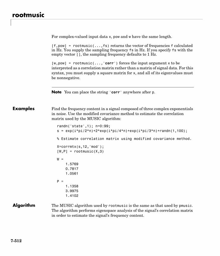
rootmusic
For complex-valued input data x, pow and w have the same length.
[f,pow] = rootmusic(...,fs) returns the vector of frequencies f calculated in Hz. You supply the sampling frequency fs in Hz. If you specify fs with the empty vector [], the sampling frequency defaults to 1 Hz.
[w,pow] = rootmusic(...,'corr') forces the input argument x to be interpreted as a correlation matrix rather than a matrix of signal data. For this syntax, you must supply a square matrix for x, and all of its eigenvalues must be nonnegative.
Note You can place the string 'corr' anywhere after p.
Examples Find the frequency content in a signal composed of three complex exponentials in noise. Use the modified covariance method to estimate the correlation matrix used by the MUSIC algorithm:
randn('state',1); n=0:99; s = exp(i*pi/2*n)+2*exp(i*pi/4*n)+exp(i*pi/3*n)+randn(1,100);
% Estimate correlation matrix using modified covariance method.
X=corrmtx(s,12,'mod'); [W,P] = rootmusic(X,3)
W = 1.5769 0.7817 1.0561
P = 1.1358 3.9975 1.4102
Algorithm The MUSIC algorithm used by rootmusic is the same as that used by pmusic. The algorithm performs eigenspace analysis of the signal’s correlation matrix in order to estimate the signal’s frequency content.
7-512
rootmusic
The difference between pmusic and rootmusic is:
• pmusic returns the pseudospectrum at all frequency samples.
• rootmusic returns the estimated discrete frequency spectrum, along with the corresponding signal power estimates.
rootmusic is most useful for frequency estimation of signals made up of a sum of sinusoids embedded in additive white Gaussian noise.
Diagnostics If the input signal, x is real and an odd number of sinusoids, p is specified, this error message is displayed
Real signals require an even number p of complex sinusoids.
See Also corrmtx, peig, pmusic, powerest method of spectrum, rooteig, spectrum.music
7-513
sawtooth
7sawtoothPurpose Generate a sawtooth or triangle wave
Syntax x = sawtooth(t)x = sawtooth(t,width)
Description sawtooth(t) generates a sawtooth wave with period 2π for the elements of time vector t. sawtooth(t) is similar to sin(t), but creates a sawtooth wave with peaks of -1 and 1 instead of a sine wave. The sawtooth wave is defined to be -1 at multiples of 2π and to increase linearly with time with a slope of 1/π at all other times.
sawtooth(t,width) generates a modified triangle wave where width, a scalar parameter between 0 and 1, determines the point between 0 and 2π at which the maximum occurs. The function increases from -1 to 1 on the interval 0 to 2π*width, then decreases linearly from 1 to -1 on the interval 2π*width to 2π. Thus a parameter of 0.5 specifies a standard triangle wave, symmetric about time instant π with peak-to-peak amplitude of 1. sawtooth(t,1) is equivalent to sawtooth(t).
See Also chirp, cos, diric, gauspuls, pulstran, rectpuls, sin, sinc, square, tripuls
7-514
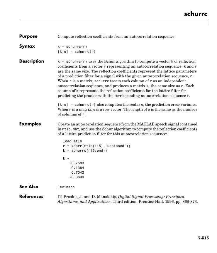
schurrc
7schurrcPurpose Compute reflection coefficients from an autocorrelation sequence
Syntax k = schurrc(r)[k,e] = schurrc(r)
Description k = schurrc(r) uses the Schur algorithm to compute a vector k of reflection coefficients from a vector r representing an autocorrelation sequence. k and r are the same size. The reflection coefficients represent the lattice parameters of a prediction filter for a signal with the given autocorrelation sequence, r. When r is a matrix, schurrc treats each column of r as an independent autocorrelation sequence, and produces a matrix k, the same size as r. Each column of k represents the reflection coefficients for the lattice filter for predicting the process with the corresponding autocorrelation sequence r.
[k,e] = schurrc(r) also computes the scalar e, the prediction error variance. When r is a matrix, e is a row vector. The length of e is the same as the number of columns of r.
Examples Create an autocorrelation sequence from the MATLAB speech signal contained in mtlb.mat, and use the Schur algorithm to compute the reflection coefficients of a lattice prediction filter for this autocorrelation sequence:
load mtlbr = xcorr(mtlb(1:5),'unbiased');k = schurrc(r(5:end))
k = -0.7583 0.1384 0.7042 -0.3699
See Also levinson
References [1] Proakis, J. and D. Manolakis, Digital Signal Processing: Principles, Algorithms, and Applications, Third edition, Prentice-Hall, 1996, pp. 868-873.
7-515
seqperiod
7seqperiodPurpose Compute the period of a sequence
Syntax p = seqperiod(x)[p,num] = seqperiod(x)
Description p = seqperiod(x) returns the integer p that corresponds to the period of the sequence in a vector x. The period p is computed as the minimum length of a subsequence x(1:p) of x that repeats itself continuously every p samples in x. The length of x does not have to be a multiple of p, so that an incomplete repetition is permitted at the end of x. If the sequence x is not periodic, then p = length(x).
• If x is a matrix, then seqperiod checks for periodicity along each column of x. The resulting output p is a row vector with the same number of columns as x.
• If x is a multidimensional array, then seqperiod checks for periodicity along the first nonsingleton dimension of x. In this case:
- p is a multidimensional array of integers with a leading singleton dimension.
- The lengths of the remaining dimensions of p correspond to those of the dimensions of x after the first nonsingleton one.
[p,num] = seqperiod(x) also returns the number num of repetitions of x(1:p) in x. num might not be an integer.
Examples x = [4 0 1 6; 2 0 2 7; 4 0 1 5; 2 0 5 6];
p = seqperiod(x)
p = 2 1 4 3
The result implies:
• The first column of x has period 2.
• The second column of x has period 1.
• The third column of x is not periodic, so p(3) is just the number of rows of x.
7-516

seqperiod
• The fourth column of x has period 3, although the last (second) repetition of the periodic sequence is incomplete.
7-517
sgolay
7sgolayPurpose Savitzky-Golay filter design
Syntax b = sgolay(k,f)b = sgolay(k,f,w)[b,g] = sgolay(...)
Description b = sgolay(k,f) designs a Savitzky-Golay FIR smoothing filter b. The polynomial order k must be less than the frame size, f, which must be odd. If k = f-1, the designed filter produces no smoothing. The output, b, is an f-by-f matrix whose rows represent the time-varying FIR filter coefficients. In a smoothing filter implementation (for example, sgolayfilt), the last (f-1)/2 rows (each an FIR filter) are applied to the signal during the startup transient, and the first (f-1)/2 rows are applied to the signal during the terminal transient. The center row is applied to the signal in the steady state.
b = sgolay(k,f,w) specifies a weighting vector w with length f, which contains the real, positive-valued weights to be used during the least-squares minimization.
[b,g] = sgolay(...) [returns the matrix g of differentiation filters. Each column of g is a differentiation filter for derivatives of order p-1 where p is the column index. Given a signal x of length f, you can find an estimate of the pth order derivative, xp, of its middle value from:
xp((f+1)/2) = (factorial(p)) * g(:,p+1)' * x
Remarks Savitzky-Golay smoothing filters (also called digital smoothing polynomial filters or least squares smoothing filters) are typically used to “smooth out” a noisy signal whose frequency span (without noise) is large. In this type of application, Savitzky-Golay smoothing filters perform much better than standard averaging FIR filters, which tend to filter out a significant portion of the signal’s high frequency content along with the noise. Although Savitzky-Golay filters are more effective at preserving the pertinent high frequency components of the signal, they are less successful than standard averaging FIR filters at rejecting noise.
Savitzky-Golay filters are optimal in the sense that they minimize the least-squares error in fitting a polynomial to each frame of noisy data.
7-518
sgolay
Examples Use sgolay to smooth a noisy sinusoid and display the result and the first and second derivatives:
N = 4;F = 21;[b,g]=sgolay(N,F);x=5*sin(.4*pi*0:.2:199);y=x+randn(1,996); % Noisy sinusoid
for n = (F+1)/2:996-(F+1)/2,% Zero-th order derivative (equivalent to sgolayfilt except% that it doesn't compute transients)
z0(n)=g(:,1)'*y(n - (F+1)/2 + 1: n + (F+1)/2 - 1)';% 1st order derivative
z1(n)=g(:,2)'*y(n - (F+1)/2 + 1: n + (F+1)/2 - 1)';% 2nd order derivative
z2(n)=2*g(:,3)'*y(n - (F+1)/2 + 1: n + (F+1)/2 - 1)';end
plot([x(1:length(z0))',y(1:length(z0))',z0'])legend('Noiseless sinusoid','Noisy sinusoid',...'Smoothed sinusoid')figureplot([diff(x(1:length(z0)+1))',z1'])legend('Noiseless first-order derivative',...'Smoothed first-order derivative')figureplot([diff(diff(x(1:length(z0)+2)))',z2'])legend('Noiseless second-order derivative',...'Smoothed second-order derivative')
Note The figures below are zoomed to show more detail.
7-519
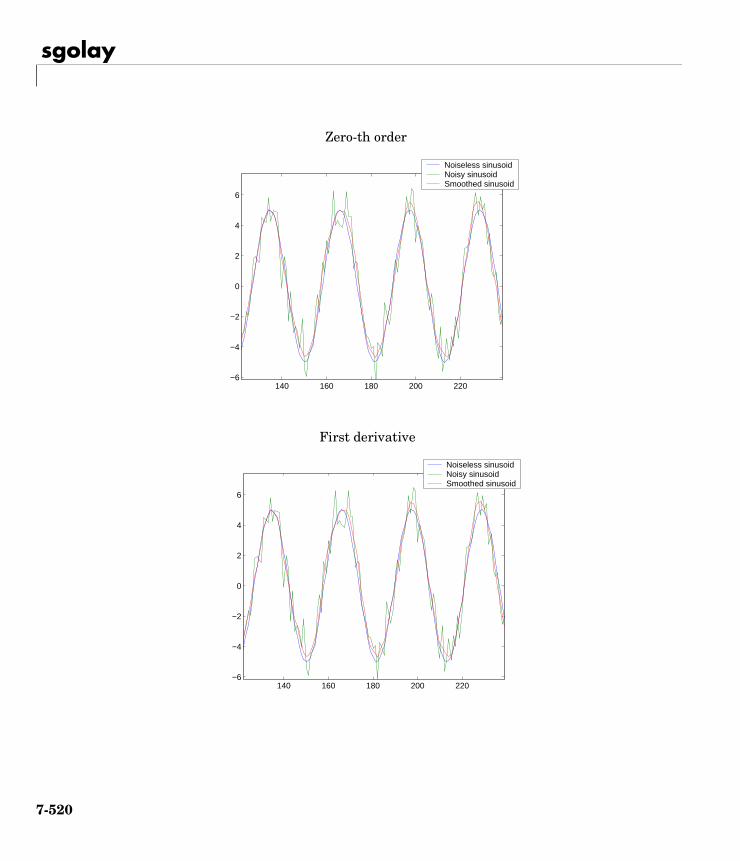
sgolay
140 160 180 200 220−6
−4
−2
0
2
4
6
Noiseless sinusoidNoisy sinusoidSmoothed sinusoid
Zero-th order
140 160 180 200 220−6
−4
−2
0
2
4
6
Noiseless sinusoidNoisy sinusoidSmoothed sinusoid
First derivative
7-520
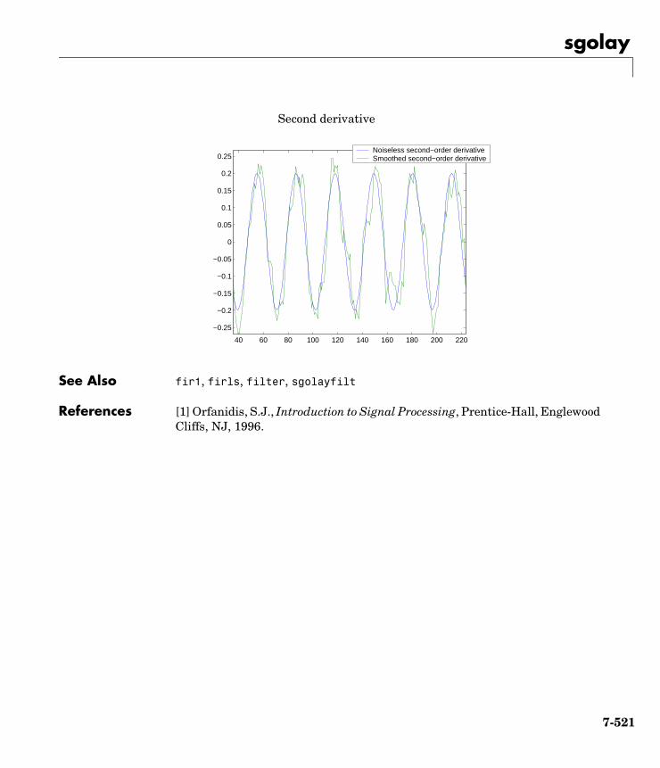
sgolay
See Also fir1, firls, filter, sgolayfilt
References [1] Orfanidis, S.J., Introduction to Signal Processing, Prentice-Hall, Englewood Cliffs, NJ, 1996.
40 60 80 100 120 140 160 180 200 220
−0.25
−0.2
−0.15
−0.1
−0.05
0
0.05
0.1
0.15
0.2
0.25Noiseless second−order derivativeSmoothed second−order derivative
Second derivative
7-521
sgolayfilt
7sgolayfiltPurpose Savitzky-Golay filtering
Syntax y = sgolayfilt(x,k,f)y = sgolayfilt(x,k,f,w)y = sgolayfilt(x,k,f,w,dim)
Description y = sgolayfilt(x,k,f) applies a Savitzky-Golay FIR smoothing filter to the data in vector x. If x is a matrix, sgolayfilt operates on each column. The polynomial order k must be less than the frame size, f, which must be odd. If k = f-1, the filter produces no smoothing.
y = sgolayfilt(x,k,f,w) specifies a weighting vector w with length f, which contains the real, positive-valued weights to be used during the least-squares minimization. If w is not specified or if it is specified as empty, [], w defaults to an identity matrix.
y = sgolayfilt(x,k,f,w,dim) specifies the dimension, dim, along which the filter operates. If dim is not specified, sgolayfilt operates along the first non-singleton dimension; that is, dimension 1 for column vectors and nontrivial matrices, and dimension 2 for row vectors.
Remarks Savitzky-Golay smoothing filters (also called digital smoothing polynomial filters or least-squares smoothing filters) are typically used to “smooth out” a noisy signal whose frequency span (without noise) is large. In this type of application, Savitzky-Golay smoothing filters perform much better than standard averaging FIR filters, which tend to filter out a significant portion of the signal’s high frequency content along with the noise. Although Savitzky-Golay filters are more effective at preserving the pertinent high frequency components of the signal, they are less successful than standard averaging FIR filters at rejecting noise.
Savitzky-Golay filters are optimal in the sense that they minimize the least-squares error in fitting a polynomial to frames of noisy data.
Examples Smooth the mtlb signal by applying a cubic Savitzky-Golay filter to data frames of length 41:
load mtlb % Load the data.smtlb = sgolayfilt(mtlb,3,41); % Apply the 3rd-order filter.
7-522
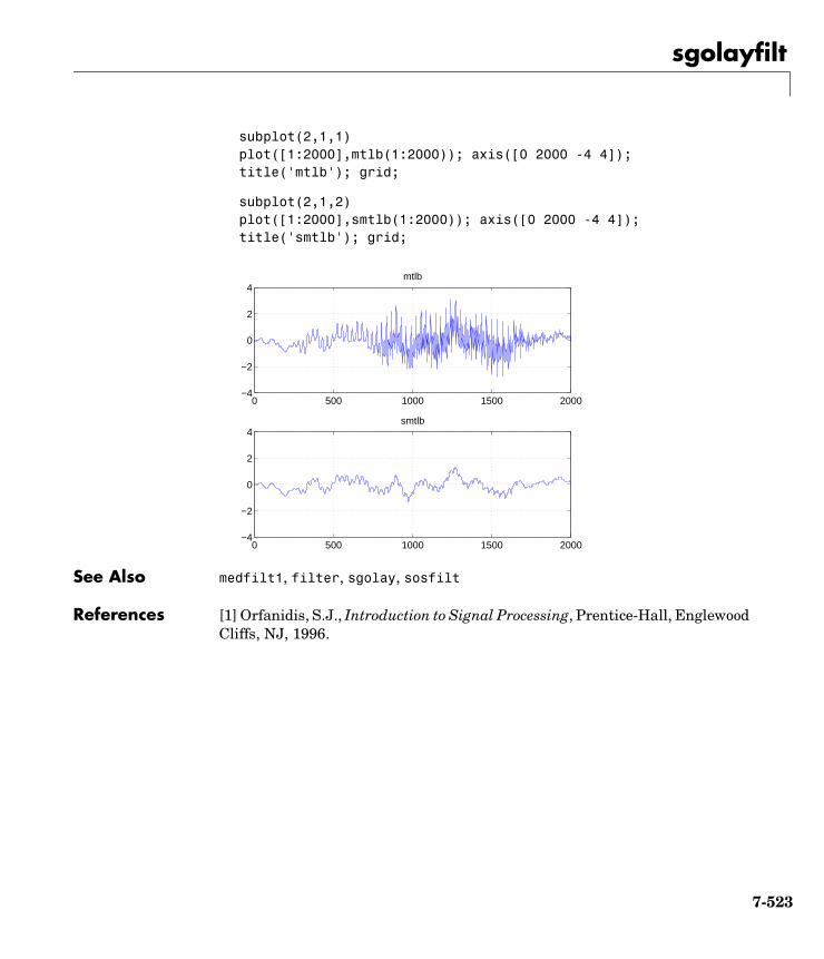
sgolayfilt
subplot(2,1,1)plot([1:2000],mtlb(1:2000)); axis([0 2000 -4 4]);title('mtlb'); grid;
subplot(2,1,2)plot([1:2000],smtlb(1:2000)); axis([0 2000 -4 4]);title('smtlb'); grid;
See Also medfilt1, filter, sgolay, sosfilt
References [1] Orfanidis, S.J., Introduction to Signal Processing, Prentice-Hall, Englewood Cliffs, NJ, 1996.
0 500 1000 1500 2000−4
−2
0
2
4mtlb
0 500 1000 1500 2000−4
−2
0
2
4smtlb
7-523
sigwin
7sigwinPurpose Construct a window object
Syntax w = sigwin.window(input1,...)
Description w = sigwin.window returns a window object, w, of type window. Each window takes one or more inputs. If you specify a sigwin.window with no inputs, a default window of length 64 is created.
Note You must use a window with sigwin.
Constructorswindow for sigwin specifies the type of window. All windows in the Signal Processing Toolbox are available for use with sigwin. For a complete list, see the window reference page.
MethodsMethods provide ways of performing functions directly on your sigwin object without having to specify the window parameters again. You can apply this method directly on the variable you assigned to your sigwin object.
Method Description
generate Returns a column vector of values representing the window.
info Returns information about the window object.
winwrite Writes an ASCII file that contains window weights for a single window object or a vector of window objects. Default filename is untitled.wf.
winwrite(Hd,filename) writes to a disk file named filename in the current working directory. The .wf extension is added automatically.
7-524
sigwin
Viewing Object ParametersAs with any object, you can use get to view a sigwin object’s parameters. To see a specific parameter,
get(w,'parameter')
or to see all parameters for an object,
get(w)
Changing Object ParametersTo set specific parameters,
set(w,'parameter1',value,'parameter2',value,...)
Note that you must use single quotation marks around the parameter name.
Examples Create a default Bartlett window and view the results in the Window Visualization Tool (wvtool). See bartlett for information on Bartlett windows:
w=sigwin.bartlett
w = Length: 64 Name: 'Bartlett'
wvtool(w)
7-525
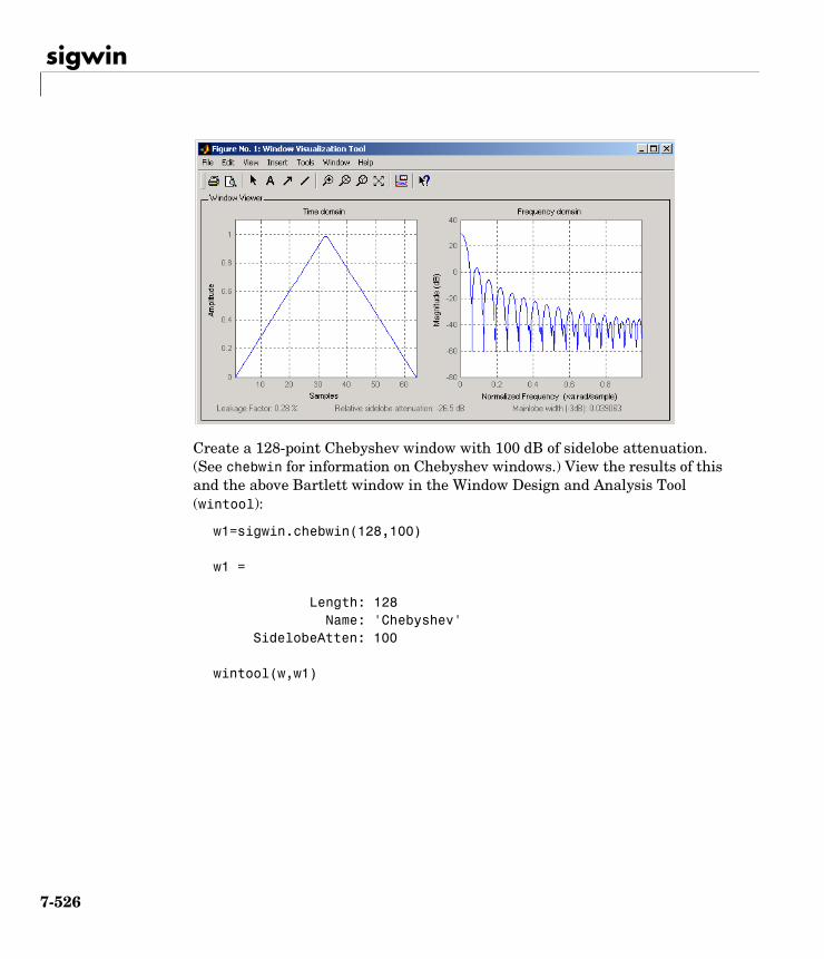
sigwin
Create a 128-point Chebyshev window with 100 dB of sidelobe attenuation. (See chebwin for information on Chebyshev windows.) View the results of this and the above Bartlett window in the Window Design and Analysis Tool (wintool):
w1=sigwin.chebwin(128,100)
w1 = Length: 128 Name: 'Chebyshev'
SidelobeAtten: 100
wintool(w,w1)
7-526
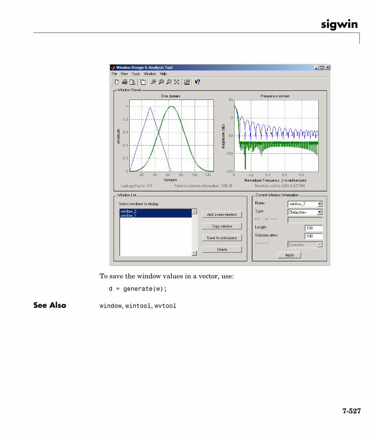
sigwin
To save the window values in a vector, use:
d = generate(w);
See Also window, wintool, wvtool
7-527
sinc
7sincPurpose Sinc function
Syntax y = sinc(x)
Description sinc computes the sinc function of an input vector or array, where the sinc function is
This function is the continuous inverse Fourier transform of the rectangular pulse of width 2π and height 1.
y = sinc(x) returns an array y the same size as x, whose elements are the sinc function of the elements of x.
The space of functions bandlimited in the frequency range is spanned by the infinite (yet countable) set of sinc functions shifted by integers. Thus any such bandlimited function g(t) can be reconstructed from its samples at integer spacings.
Examples Perform ideal bandlimited interpolation by assuming that the signal to be interpolated is 0 outside of the given time interval and that it has been sampled at exactly the Nyquist frequency:
t = (1:10)'; % A column vector of time samplesrandn('state',0);x = randn(size(t)); % A column vector of data
ts = linspace(-5,15,600)'; % times at which to interpolate data
sinc t( )1 t 0=,
πt( )sinπt
------------------- t 0≠,
=
sinc t( )1
2π------ ejωt ωd
π–
π
∫=
ω π– π[ , ]∈
g t( ) g n( )sinc t n–( )
n ∞–=
∞
∑=
7-528
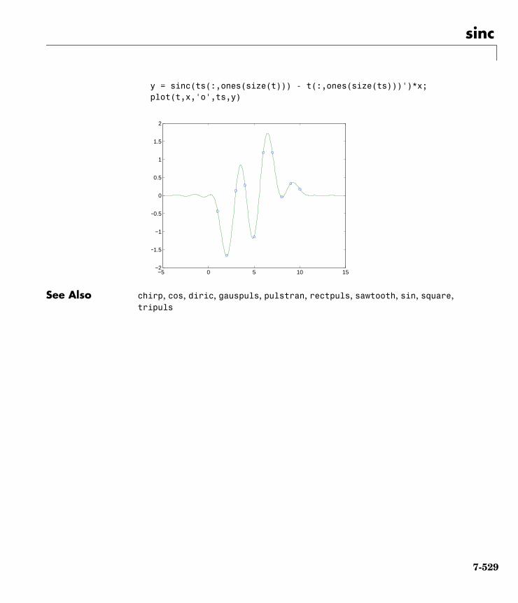
sinc
y = sinc(ts(:,ones(size(t))) - t(:,ones(size(ts)))')*x;plot(t,x,'o',ts,y)
See Also chirp, cos, diric, gauspuls, pulstran, rectpuls, sawtooth, sin, square, tripuls
−5 0 5 10 15−2
−1.5
−1
−0.5
0
0.5
1
1.5
2
7-529

sos2cell
7sos2cellPurpose Convert a second-order section matrix to cell arrays
Syntax c = sos2cell(m)
c = sos2cell(m,g)
Description c = sos2cell(m) changes an L-by-6 second-order section matrix m generated by tf2sos into a 1-by-L cell array of 1-by-2 cell arrays c. You can use c to specify a quantized filter with L cascaded second-order sections.
The matrix m should have the form
m = [b1 a1;b2 a2; ... ;bL aL]
where both bi and ai, with i = 1, ..., L, are 1-by-3 row vectors. The resulting c is a 1-by-L cell array of cells of the form
c = b1 a1 b2 a2 ... bL aL
c = sos2cell(m,g) with the optional gain term g, prepends the constant value g to c. When you use the added gain term in the command, c is a 1-by-L cell array of cells of the form
c = g,1 b1,a1 b2,a2...bL,aL
Examples Use sos2cell to convert the 2-by-6 second-order section matrix produced by tf2sos into a 1-by-2 cell array c of cells. Display the second entry in the first cell in c:
[b,a] = ellip(4,0.5,20,0.6);m = tf2sos(b,a);c = sos2cell(m);c12
ans =
1.0000 0.1677 0.2575
See Also tf2sos, cell2sos
7-530
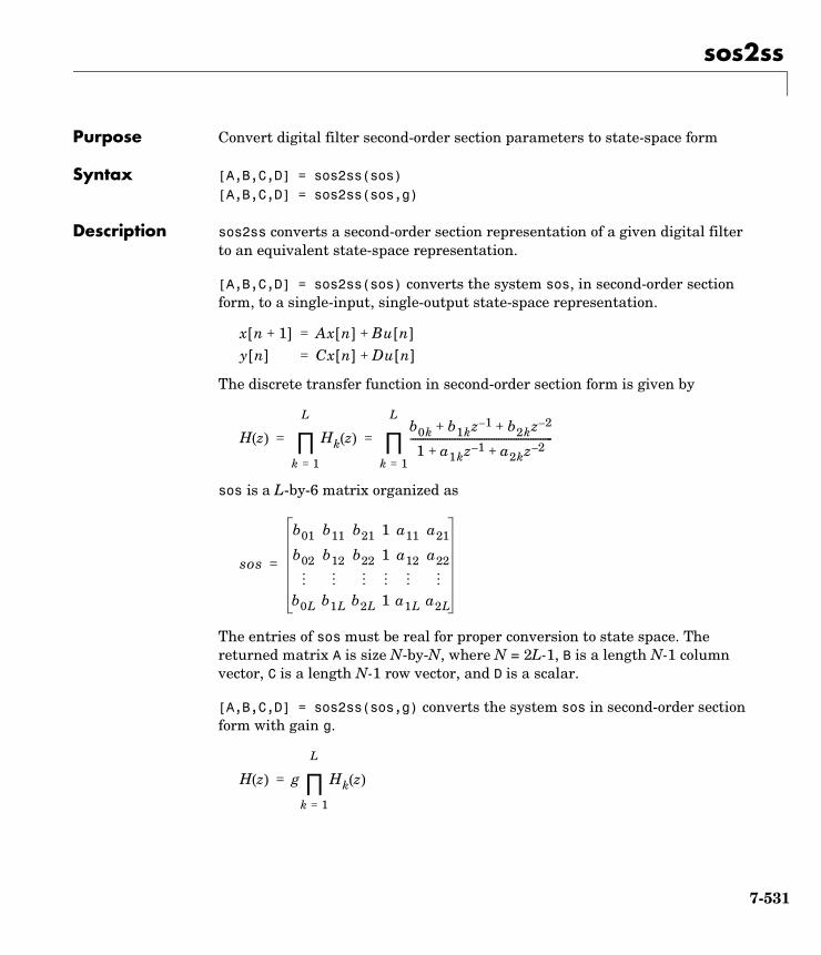
sos2ss
7sos2ssPurpose Convert digital filter second-order section parameters to state-space form
Syntax [A,B,C,D] = sos2ss(sos)[A,B,C,D] = sos2ss(sos,g)
Description sos2ss converts a second-order section representation of a given digital filter to an equivalent state-space representation.
[A,B,C,D] = sos2ss(sos) converts the system sos, in second-order section form, to a single-input, single-output state-space representation.
The discrete transfer function in second-order section form is given by
sos is a L-by-6 matrix organized as
The entries of sos must be real for proper conversion to state space. The returned matrix A is size N-by-N, where N = 2L-1, B is a length N-1 column vector, C is a length N-1 row vector, and D is a scalar.
[A,B,C,D] = sos2ss(sos,g) converts the system sos in second-order section form with gain g.
x n 1+[ ] Ax n[ ] Bu n[ ]+=
y n[ ] Cx n[ ] Du n[ ]+=
H z( ) Hk z( )
k 1=
L
∏b0k b1kz 1– b2kz 2–+ +
1 a1kz 1– a2kz 2–+ +----------------------------------------------------------
k 1=
L
∏= =
sos
b01 b11 b21 1 a11 a21
b02 b12 b22 1 a12 a22
b0L b1L b2L 1 a1L a2L
=
H z( ) g Hk z( )
k 1=
L
∏=
7-531
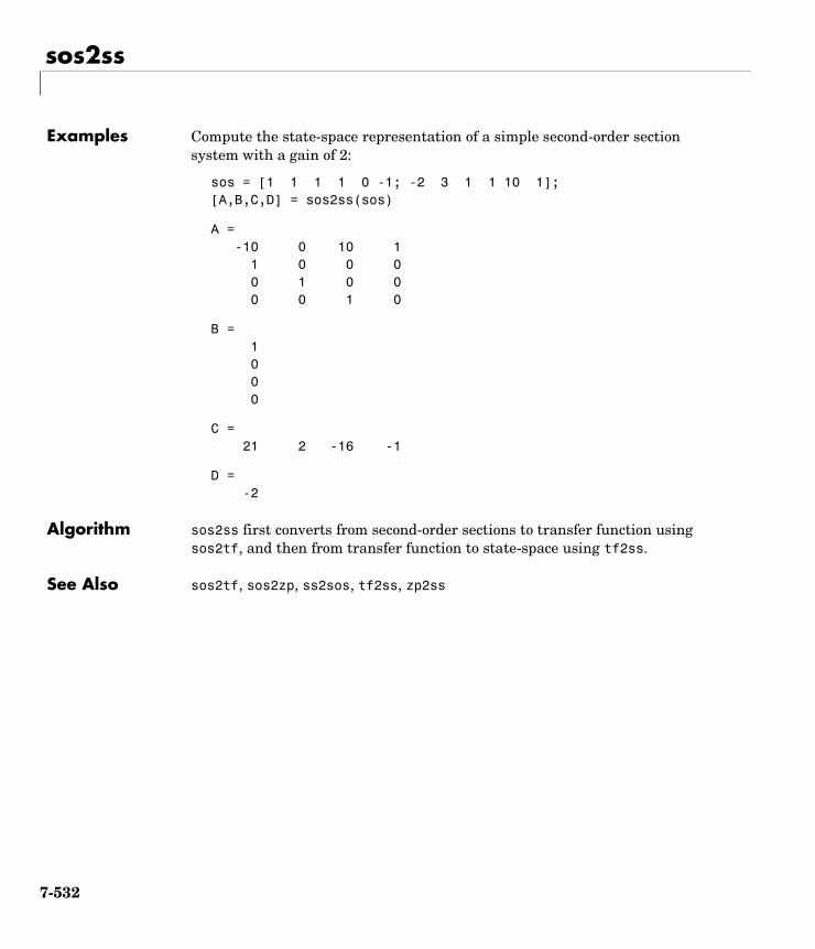
sos2ss
Examples Compute the state-space representation of a simple second-order section system with a gain of 2:
sos = [1 1 1 1 0 -1; -2 3 1 1 10 1];[A,B,C,D] = sos2ss(sos)
A = -10 0 10 1 1 0 0 0 0 1 0 0 0 0 1 0
B = 1 0 0 0
C = 21 2 -16 -1
D = -2
Algorithm sos2ss first converts from second-order sections to transfer function using sos2tf, and then from transfer function to state-space using tf2ss.
See Also sos2tf, sos2zp, ss2sos, tf2ss, zp2ss
7-532
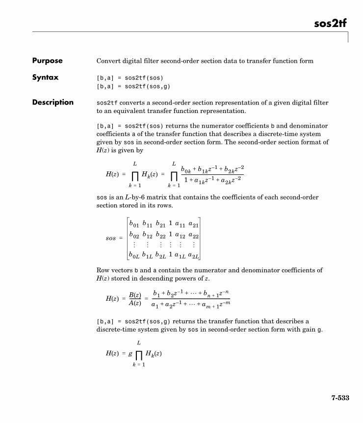
sos2tf
7sos2tfPurpose Convert digital filter second-order section data to transfer function form
Syntax [b,a] = sos2tf(sos)[b,a] = sos2tf(sos,g)
Description sos2tf converts a second-order section representation of a given digital filter to an equivalent transfer function representation.
[b,a] = sos2tf(sos) returns the numerator coefficients b and denominator coefficients a of the transfer function that describes a discrete-time system given by sos in second-order section form. The second-order section format of H(z) is given by
sos is an L-by-6 matrix that contains the coefficients of each second-order section stored in its rows.
Row vectors b and a contain the numerator and denominator coefficients of H(z) stored in descending powers of z.
[b,a] = sos2tf(sos,g) returns the transfer function that describes a discrete-time system given by sos in second-order section form with gain g.
H z( ) Hk z( )
k 1=
L
∏b0k b1kz 1– b2kz 2–+ +
1 a1kz 1– a2kz 2–+ +----------------------------------------------------------
k 1=
L
∏= =
sos
b01 b11 b21 1 a11 a21
b02 b12 b22 1 a12 a22
b0L b1L b2L 1 a1L a2L
=
H z( )B z( )A z( )-----------
b1 b2z 1– bn 1+ z n–+ + +
a1 a2z 1– am 1+ z m–+ + +------------------------------------------------------------------------= =
H z( ) g Hk z( )
k 1=
L
∏=
7-533
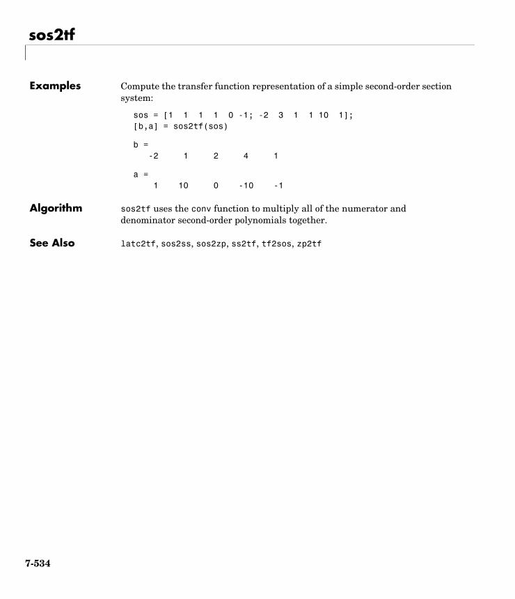
sos2tf
Examples Compute the transfer function representation of a simple second-order section system:
sos = [1 1 1 1 0 -1; -2 3 1 1 10 1];[b,a] = sos2tf(sos)
b = -2 1 2 4 1
a = 1 10 0 -10 -1
Algorithm sos2tf uses the conv function to multiply all of the numerator and denominator second-order polynomials together.
See Also latc2tf, sos2ss, sos2zp, ss2tf, tf2sos, zp2tf
7-534
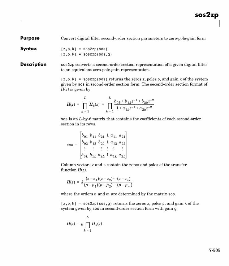
sos2zp
7sos2zpPurpose Convert digital filter second-order section parameters to zero-pole-gain form
Syntax [z,p,k] = sos2zp(sos)[z,p,k] = sos2zp(sos,g)
Description sos2zp converts a second-order section representation of a given digital filter to an equivalent zero-pole-gain representation.
[z,p,k] = sos2zp(sos) returns the zeros z, poles p, and gain k of the system given by sos in second-order section form. The second-order section format of H(z) is given by
sos is an L-by-6 matrix that contains the coefficients of each second-order section in its rows.
Column vectors z and p contain the zeros and poles of the transfer function H(z).
where the orders n and m are determined by the matrix sos.
[z,p,k] = sos2zp(sos,g) returns the zeros z, poles p, and gain k of the system given by sos in second-order section form with gain g.
H z( ) Hk z( )
k 1=
L
∏b0k b1kz 1– b2kz 2–+ +
1 a1kz 1– a2kz 2–+ +----------------------------------------------------------
k 1=
L
∏= =
sos
b01 b11 b21 1 a11 a21
b02 b12 b22 1 a12 a22
b0L b1L b2L 1 a1L a2L
=
H z( ) kz z1–( ) z z2–( ) z zn–( )
p p1–( ) p p2–( ) p pm–( )----------------------------------------------------------------------=
H z( ) g Hk z( )
k 1=
L
∏=
7-535
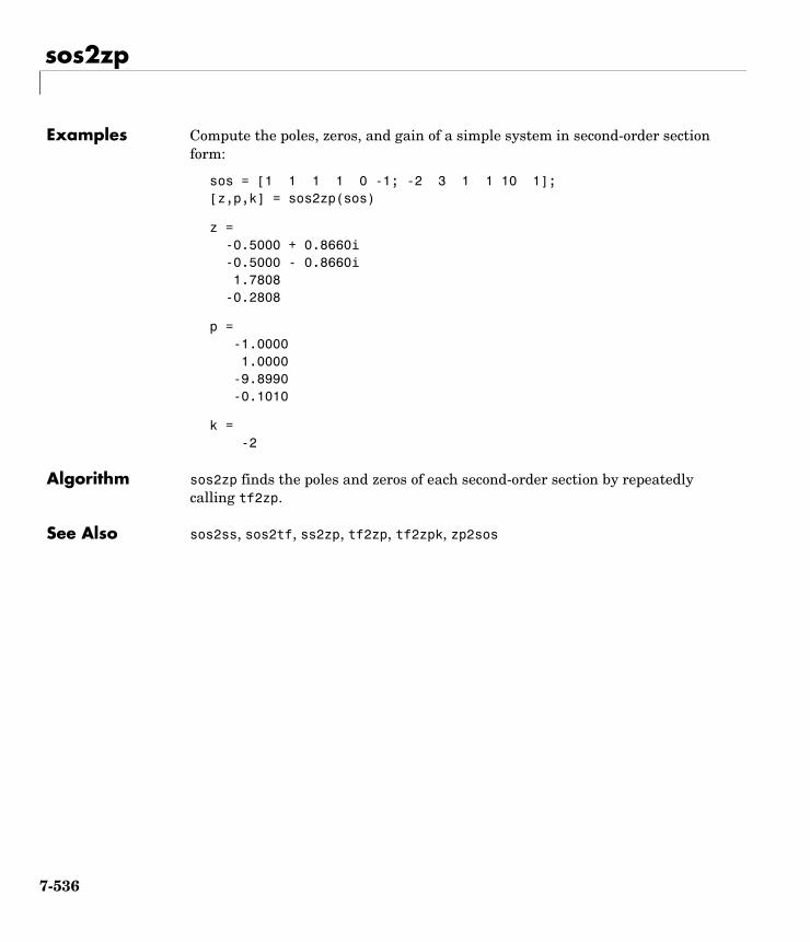
sos2zp
Examples Compute the poles, zeros, and gain of a simple system in second-order section form:
sos = [1 1 1 1 0 -1; -2 3 1 1 10 1];[z,p,k] = sos2zp(sos)
z = -0.5000 + 0.8660i -0.5000 - 0.8660i 1.7808 -0.2808
p = -1.0000 1.0000 -9.8990 -0.1010
k = -2
Algorithm sos2zp finds the poles and zeros of each second-order section by repeatedly calling tf2zp.
See Also sos2ss, sos2tf, ss2zp, tf2zp, tf2zpk, zp2sos
7-536
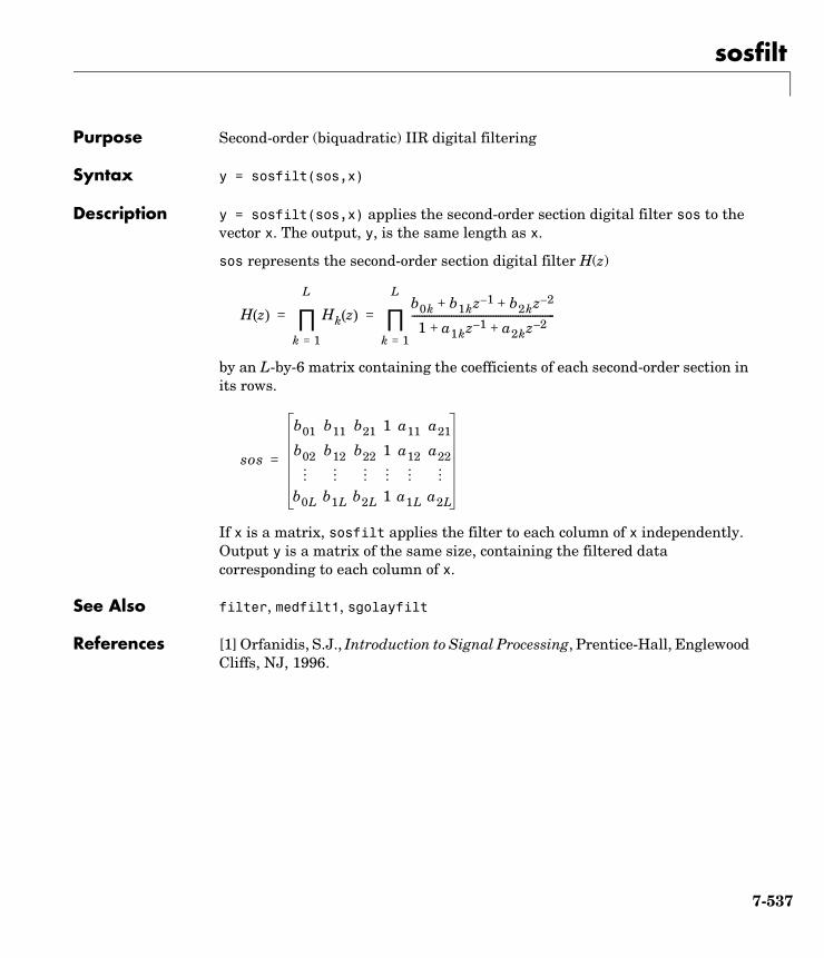
sosfilt
7sosfiltPurpose Second-order (biquadratic) IIR digital filtering
Syntax y = sosfilt(sos,x)
Description y = sosfilt(sos,x) applies the second-order section digital filter sos to the vector x. The output, y, is the same length as x.
sos represents the second-order section digital filter H(z)
by an L-by-6 matrix containing the coefficients of each second-order section in its rows.
If x is a matrix, sosfilt applies the filter to each column of x independently. Output y is a matrix of the same size, containing the filtered data corresponding to each column of x.
See Also filter, medfilt1, sgolayfilt
References [1] Orfanidis, S.J., Introduction to Signal Processing, Prentice-Hall, Englewood Cliffs, NJ, 1996.
H z( ) Hk z( )
k 1=
L
∏b0k b1kz 1– b2kz 2–+ +
1 a1kz 1– a2kz 2–+ +----------------------------------------------------------
k 1=
L
∏= =
sos
b01 b11 b21 1 a11 a21
b02 b12 b22 1 a12 a22
b0L b1L b2L 1 a1L a2L
=
7-537
specgram
7specgramPurpose Time-dependent frequency analysis (spectrogram)
Syntax B = specgram(a)B = specgram(a,nfft)[B,f] = specgram(a,nfft,fs)[B,f,t] = specgram(a,nfft,fs)B = specgram(a,nfft,fs,window)B = specgram(a,nfft,fs,window,numoverlap)specgram(a)B = specgram(a,f,fs,window,numoverlap)
Description specgram computes the windowed discrete-time Fourier transform of a signal using a sliding window. The spectrogram is the magnitude of this function.
B = specgram(a) calculates the windowed discrete-time Fourier transform for the signal in vector a. This syntax uses the default values:
• nfft = min(256,length(a)) • fs = 2
• window is a periodic Hann (Hanning) window of length nfft.• numoverlap = length(window)/2
nfft specifies the FFT length that specgram uses. This value determines the frequencies at which the discrete-time Fourier transform is computed. fs is a scalar that specifies the sampling frequency. window specifies a windowing function and the number of samples specgram uses in its sectioning of vector a. numoverlap is the number of samples by which the sections overlap. Any arguments that you omit from the end of the input parameter list use the default values shown above.
If a is real, specgram computes the discrete-time Fourier transform at positive frequencies only. If n is even, specgram returns nfft/2+1 rows (including the zero and Nyquist frequency terms). If n is odd, specgram returns nfft/2 rows. The number of columns in B is
k = fix((n-numoverlap)/(length(window)-numoverlap))
If a is complex, specgram computes the discrete-time Fourier transform at both positive and negative frequencies. In this case, B is a complex matrix with nfft
7-538
specgram
rows. Time increases linearly across the columns of B, starting with sample 1 in column 1. Frequency increases linearly down the rows, starting at 0.
B = specgram(a,nfft) uses the specified FFT length nfft in its calculations.
[B,f] = specgram(a,nfft,fs) returns a vector f of frequencies at which the function computes the discrete-time Fourier transform. fs has no effect on the output B; it is a frequency scaling multiplier.
[B,f,t] = specgram(a,nfft,fs) returns frequency and time vectors f and t respectively. t is a column vector of scaled times, with length equal to the number of columns of B. t(j) is the earliest time at which the jth window intersects a. t(1) is always equal to 0.
B = specgram(a,nfft,fs,window) specifies a windowing function and the number of samples per section of the x vector. If you supply a scalar for window, specgram uses a Hann window of that length. The length of the window must be less than or equal to nfft.
B = specgram(a,nfft,fs,window,numoverlap) overlaps the sections of x by numoverlap samples.
You can use the empty matrix [] to specify the default value for any input argument. For example,
B = specgram(x,[],10000)
is equivalent to
B = specgram(x)
but with a sampling frequency of 10,000 Hz instead of the default 2 Hz.
specgram(...) with no output arguments displays the scaled logarithm of the spectrogram in the current figure window using
imagesc(t,f,20*log10(abs(b))), axis xy, colormap(jet)
The axis xy mode displays the low-frequency content of the first portion of the signal in the lower-left corner of the axes. specgram uses fs to label the axes according to true time and frequency.
7-539
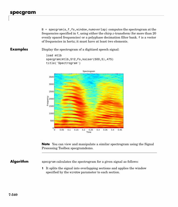
specgram
B = specgram(a,f,fs,window,numoverlap) computes the spectrogram at the frequencies specified in f, using either the chirp z-transform (for more than 20 evenly spaced frequencies) or a polyphase decimation filter bank. f is a vector of frequencies in hertz; it must have at least two elements.
Examples Display the spectrogram of a digitized speech signal:
load mtlbspecgram(mtlb,512,Fs,kaiser(500,5),475)title('Spectrogram')
Note You can view and manipulate a similar spectrogram using the Signal Processing Toolbox specgramdemo.
Algorithm specgram calculates the spectrogram for a given signal as follows:
1 It splits the signal into overlapping sections and applies the window specified by the window parameter to each section.
Time
Fre
quen
cy
Spectrogram
0 0.05 0.1 0.15 0.2 0.25 0.3 0.35 0.4 0.450
500
1000
1500
2000
2500
3000
3500
7-540
specgram
2 It computes the discrete-time Fourier transform of each section with a length nfft FFT to produce an estimate of the short-term frequency content of the signal; these transforms make up the columns of B. The quantity (length(window) - numoverlap) specifies by how many samples specgram shifts the window.
3 For real input, specgram truncates the spectrogram to the first nfft/2 + 1 points for nfft even and (nfft + 1)/2 for nfft odd.
Diagnostics An appropriate diagnostic message is displayed when incorrect arguments are used:
Requires window's length to be no greater than the FFT length.Requires NOVERLAP to be strictly less than the window length.Requires positive integer values for NFFT and NOVERLAP.Requires vector input.
See Also mscohere, cpsd, pwelch, tfestimate
References [1] Oppenheim, A.V., and R.W. Schafer, Discrete-Time Signal Processing, Prentice-Hall, Englewood Cliffs, NJ, 1989, pp. 713-718.
[2] Rabiner, L.R., and R.W. Schafer, Digital Processing of Speech Signals, Prentice-Hall, Englewood Cliffs, NJ, 1978.
7-541
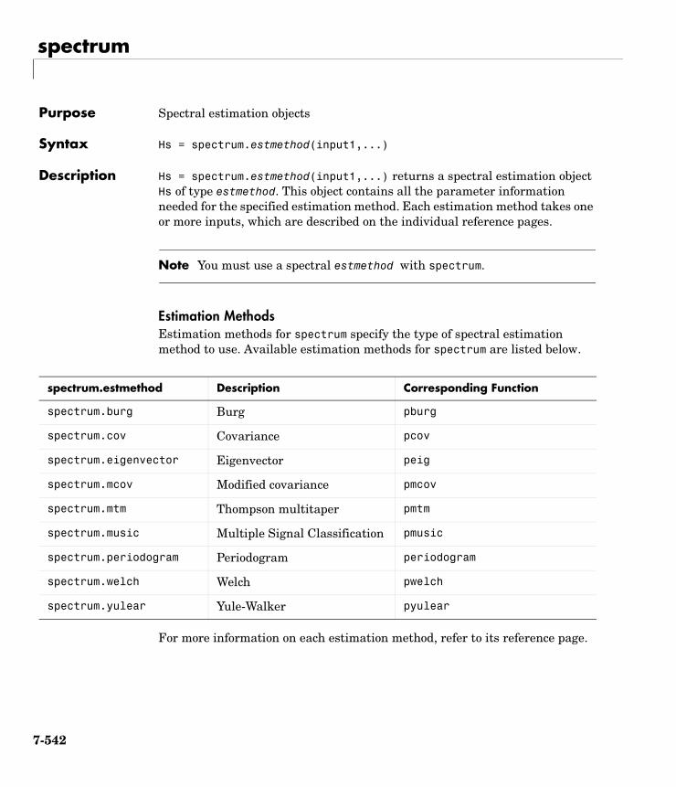
spectrum
7spectrumPurpose Spectral estimation objects
Syntax Hs = spectrum.estmethod(input1,...)
Description Hs = spectrum.estmethod(input1,...) returns a spectral estimation object Hs of type estmethod. This object contains all the parameter information needed for the specified estimation method. Each estimation method takes one or more inputs, which are described on the individual reference pages.
Note You must use a spectral estmethod with spectrum.
Estimation MethodsEstimation methods for spectrum specify the type of spectral estimation method to use. Available estimation methods for spectrum are listed below.
For more information on each estimation method, refer to its reference page.
spectrum.estmethod Description Corresponding Function
spectrum.burg Burg pburg
spectrum.cov Covariance pcov
spectrum.eigenvector Eigenvector peig
spectrum.mcov Modified covariance pmcov
spectrum.mtm Thompson multitaper pmtm
spectrum.music Multiple Signal Classification pmusic
spectrum.periodogram Periodogram periodogram
spectrum.welch Welch pwelch
spectrum.yulear Yule-Walker pyulear
7-542

spectrum
Note For estimation methods that use overlap and window length inputs, you specify the number of overlap samples as a percent overlap and you specify the segment length instead of the window length.
For estimation methods that use windows, if the window uses an additional parameter, a property is dynamically added to the spectrum object for that parameter. You can change that property using set (see Changing Object Properties on page 550).
MethodsMethods provide ways of performing functions directly on your spectrum object without having to specify the spectral estimation parameters again. You can apply these methods directly on the variable you assigned to your spectrum object. For more information on any of these methods, use the syntax help spectrum/estmethod at the MATLAB prompt.
7-543
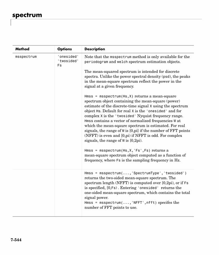
spectrum
Method Options Description
msspectrum 'onesided''twosided'Fs
Note that the msspectrum method is only available for the periodogram and welch spectrum estimation objects.
The mean-squared spectrum is intended for discrete spectra. Unlike the power spectral density (psd), the peaks in the mean-square spectrum reflect the power in the signal at a given frequency.
Hmss = msspectrum(Hs,X) returns a mean-square spectrum object containing the mean-square (power) estimate of the discrete-time signal X using the spectrum object Hs. Default for real X is the 'onesided' and for complex X is the 'twosided' Nyquist frequency range. Hmss contains a vector of normalized frequencies W at which the mean-sqaure spectrum is estimated. For real signals, the range of W is [0,pi] if the number of FFT points (NFFT) is even and [0,pi) if NFFT is odd. For complex signals, the range of W is [0,2pi).
Hmss = msspectrum(Hs,X,'Fs',Fs) returns a mean-square spectrum object computed as a function of frequency, where Fs is the sampling frequency in Hz.
Hmss = msspectrum(...,'SpectrumType','twosided') returns the two-sided mean-square spectrum. The spectrum length (NFFT) is computed over [0,2pi), or if Fs is specified, [0,Fs) . Entering 'onesided' returns the one-sided mean-square spectrum, which contains the total signal power.Hmss = msspectrum(...,'NFFT',nfft) specifes the number of FFT points to use.
7-544
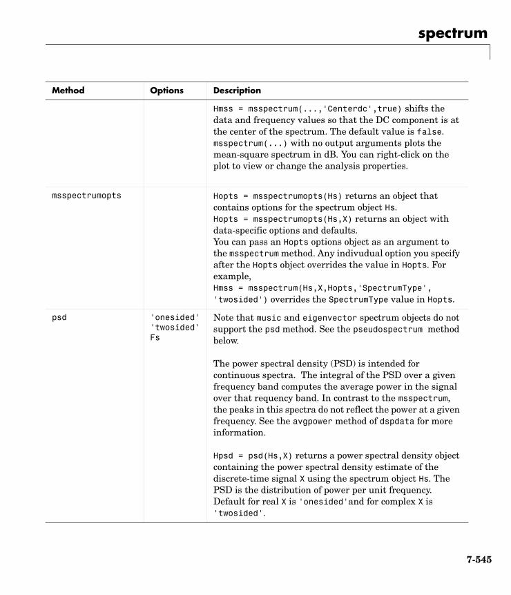
spectrum
Hmss = msspectrum(...,'Centerdc',true) shifts the data and frequency values so that the DC component is at the center of the spectrum. The default value is false.msspectrum(...) with no output arguments plots the mean-square spectrum in dB. You can right-click on the plot to view or change the analysis properties.
msspectrumopts Hopts = msspectrumopts(Hs) returns an object that contains options for the spectrum object Hs.Hopts = msspectrumopts(Hs,X) returns an object with data-specific options and defaults.You can pass an Hopts options object as an argument to the msspectrum method. Any indivudual option you specify after the Hopts object overrides the value in Hopts. For example, Hmss = msspectrum(Hs,X,Hopts,'SpectrumType', 'twosided') overrides the SpectrumType value in Hopts.
psd 'onesided''twosided'Fs
Note that music and eigenvector spectrum objects do not support the psd method. See the pseudospectrum method below.
The power spectral density (PSD) is intended for continuous spectra. The integral of the PSD over a given frequency band computes the average power in the signal over that requency band. In contrast to the msspectrum, the peaks in this spectra do not reflect the power at a given frequency. See the avgpower method of dspdata for more information.
Hpsd = psd(Hs,X) returns a power spectral density object containing the power spectral density estimate of the discrete-time signal X using the spectrum object Hs. The PSD is the distribution of power per unit frequency. Default for real X is 'onesided'and for complex X is 'twosided'.
Method Options Description
7-545
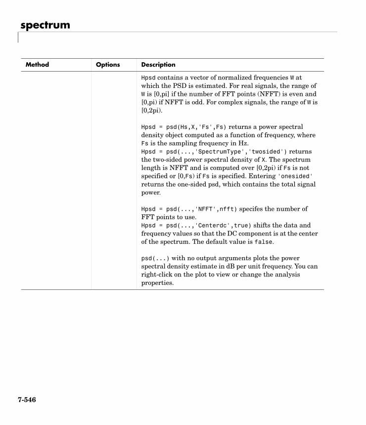
spectrum
Hpsd contains a vector of normalized frequencies W at which the PSD is estimated. For real signals, the range of W is [0,pi] if the number of FFT points (NFFT) is even and [0,pi) if NFFT is odd. For complex signals, the range of W is [0,2pi).
Hpsd = psd(Hs,X,'Fs',Fs) returns a power spectral density object computed as a function of frequency, where Fs is the sampling frequency in Hz.Hpsd = psd(...,'SpectrumType','twosided') returns the two-sided power spectral density of X. The spectrum length is NFFT and is computed over [0,2pi) if Fs is not specified or [0,Fs) if Fs is specified. Entering 'onesided' returns the one-sided psd, which contains the total signal power.
Hpsd = psd(...,'NFFT',nfft) specifes the number of FFT points to use.Hpsd = psd(...,'Centerdc',true) shifts the data and frequency values so that the DC component is at the center of the spectrum. The default value is false.
psd(...) with no output arguments plots the power spectral density estimate in dB per unit frequency. You can right-click on the plot to view or change the analysis properties.
Method Options Description
7-546
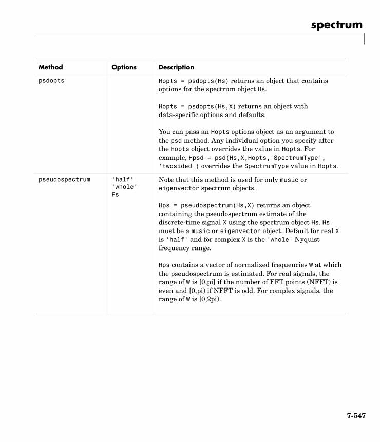
spectrum
psdopts Hopts = psdopts(Hs) returns an object that contains options for the spectrum object Hs.
Hopts = psdopts(Hs,X) returns an object with data-specific options and defaults.
You can pass an Hopts options object as an argument to the psd method. Any individual option you specify after the Hopts object overrides the value in Hopts. For example, Hpsd = psd(Hs,X,Hopts,'SpectrumType', 'twosided') overrides the SpectrumType value in Hopts.
pseudospectrum 'half''whole'Fs
Note that this method is used for only music or eigenvector spectrum objects.
Hps = pseudospectrum(Hs,X) returns an object containing the pseudospectrum estimate of the discrete-time signal X using the spectrum object Hs. Hs must be a music or eigenvector object. Default for real X is 'half' and for complex X is the 'whole' Nyquist frequency range.
Hps contains a vector of normalized frequencies W at which the pseudospectrum is estimated. For real signals, the range of W is [0,pi] if the number of FFT points (NFFT) is even and [0,pi) if NFFT is odd. For complex signals, the range of W is [0,2pi).
Method Options Description
7-547

spectrum
Hps = pseudospectrum(Hs,X,'Fs',Fs) returns a pseudospectrum object computed as a function of frequency, where Fs is the sampling frequency in Hz.Hmps = pseudospectrum(...,'SpectrumRange','whole') returns the pseudospectrum over the whole Nyquist range. The spectrum length is NFFT and is computed over [0,2pi) if Fs is not specified or [0,Fs) if Fs is specified. Entering 'half' returns the pseudospectrum calculated over half the Nyquist range.
Hps = pseudospectrum(...,'NFFT',nfft) specifes the number of FFT points to use
Hps = pseudospectrum(...,'Centerdc',true) shifts the data and frequency values so that the DC component is at the center of the spectrum. The default value is false.pseudospectrum(...) with no output arguments plots the pseudospectrum in dB. You can right-click on the plot to view or change the analysis properties.
Method Options Description
7-548
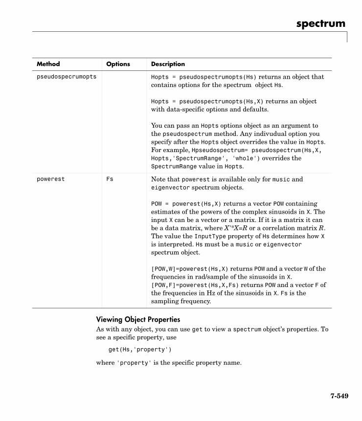
spectrum
Viewing Object PropertiesAs with any object, you can use get to view a spectrum object’s properties. To see a specific property, use
get(Hs,'property')
where 'property' is the specific property name.
pseudospecrumopts Hopts = pseudospectrumopts(Hs) returns an object that contains options for the spectrum object Hs.
Hopts = pseudospectrumopts(Hs,X) returns an object with data-specific options and defaults.
You can pass an Hopts options object as an argument to the pseudospectrum method. Any indivudual option you specify after the Hopts object overrides the value in Hopts. For example, Hpseudospectrum= pseudospectrum(Hs,X,Hopts,'SpectrumRange', 'whole') overrides the SpectrumRange value in Hopts.
powerest Fs Note that powerest is available only for music and eigenvector spectrum objects.
POW = powerest(Hs,X) returns a vector POW containing estimates of the powers of the complex sinusoids in X. The input X can be a vector or a matrix. If it is a matrix it can be a data matrix, where X'*X=R or a correlation matrix R. The value the InputType property of Hs determines how X is interpreted. Hs must be a music or eigenvector spectrum object.
[POW,W]=powerest(Hs,X) returns POW and a vector W of the frequencies in rad/sample of the sinusoids in X. [POW,F]=powerest(Hs,X,Fs) returns POW and a vector F of the frequencies in Hz of the sinusoids in X. Fs is the sampling frequency.
Method Options Description
7-549
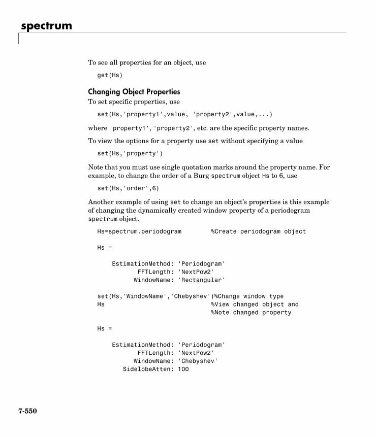
spectrum
To see all properties for an object, use
get(Hs)
Changing Object PropertiesTo set specific properties, use
set(Hs,'property1',value, 'property2',value,...)
where 'property1', 'property2', etc. are the specific property names.
To view the options for a property use set without specifying a value
set(Hs,'property')
Note that you must use single quotation marks around the property name. For example, to change the order of a Burg spectrum object Hs to 6, use
set(Hs,'order',6)
Another example of using set to change an object’s properties is this example of changing the dynamically created window property of a periodogram spectrum object.
Hs=spectrum.periodogram %Create periodogram object
Hs =
EstimationMethod: 'Periodogram' FFTLength: 'NextPow2' WindowName: 'Rectangular'
set(Hs,'WindowName','Chebyshev')%Change window typeHs %View changed object and
%Note changed property
Hs =
EstimationMethod: 'Periodogram' FFTLength: 'NextPow2' WindowName: 'Chebyshev' SidelobeAtten: 100
7-550
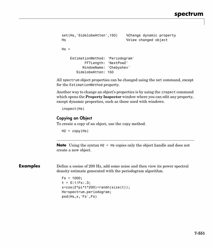
spectrum
set(Hs,'SidelobeAtten',150) %Change dynamic propertyHs %View changed object
Hs =
EstimationMethod: 'Periodogram' FFTLength: 'NextPow2' WindowName: 'Chebyshev' SidelobeAtten: 150
All spectrum object properties can be changed using the set command, except for the EstimationMethod property.
Another way to change an object’s properties is by using the inspect command which opens the Property Inspector window where you can edit any property, except dynamic properties, such as those used with windows.
inspect(Hs)
Copying an ObjectTo create a copy of an object, use the copy method.
H2 = copy(Hs)
Note Using the syntax H2 = Hs copies only the object handle and does not create a new object.
Examples Define a cosine of 200 Hz, add some noise and then view its power spectral density estimate generated with the periodogram algorithm.
Fs = 1000;t = 0:1/Fs:.3;x=cos(2*pi*t*200)+randn(size(t));Hs=spectrum.periodogram;psd(Hs,x,'Fs',Fs)
7-551
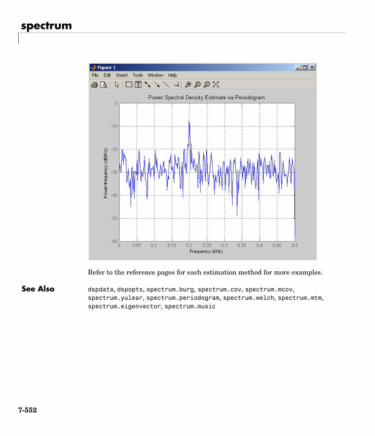
spectrum
Refer to the reference pages for each estimation method for more examples.
See Also dspdata, dspopts, spectrum.burg, spectrum.cov, spectrum.mcov, spectrum.yulear, spectrum.periodogram, spectrum.welch, spectrum.mtm, spectrum.eigenvector, spectrum.music
7-552
spectrum.burg
7spectrum.burgPurpose Construct a Burg spectrum object
Syntax Hs = spectrum.burgHs = spectrum.burg(order)Hs = spectrum.burg(order,FFTLength)
Description Hs = spectrum.burg returns a default Burg spectrum object, Hs, that defines the parameters for the Burg parametric spectral estimation algorithm. The Burg algorithm estimates the spectral content by fitting an auto-regressive (AR) linear prediction filter model of a given order to the signal.
Hs = spectrum.burg(order) returns a spectrum object, Hs with the specified order and the FFTLength determined using NextPow2. The default value for order is 4.
Hs = spectrum.burg(order,FFTLength) returns a spectrum object, Hs with the specified order of the AR model and the specified way of determining the FFTLength. Valid values of the FFTLength string are:
Note See pburg for more information on the Burg algorithm.
Examples Define a fourth order auto-regressive model and view its power spectral density using the Burg algorithm.
randn('state',1);
FFTLength string Description
'InputLength' Use the length of the input signal as the FFT length
'NextPow2' Use the next power of two greater than the input signal length as the FFT length. This is the default value.
'UserDefined' Use the FFT length provided as an input to the psd method or via a dspopts object.
7-553
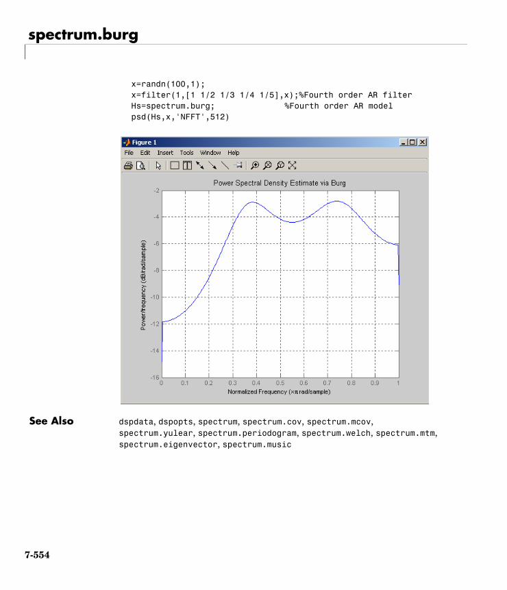
spectrum.burg
x=randn(100,1);x=filter(1,[1 1/2 1/3 1/4 1/5],x);%Fourth order AR filterHs=spectrum.burg; %Fourth order AR modelpsd(Hs,x,'NFFT',512)
See Also dspdata, dspopts, spectrum, spectrum.cov, spectrum.mcov, spectrum.yulear, spectrum.periodogram, spectrum.welch, spectrum.mtm, spectrum.eigenvector, spectrum.music
7-554
spectrum.cov
7spectrum.covPurpose Construct a covariance spectrum object
Syntax Hs = spectrum.covHs = spectrum.cov(order)Hs = spectrum.cov(order,FFTLength)
Description Hs = spectrum.cov returns a default covariance spectrum object, Hs, that defines the parameters for the covariance spectral estimation algorithm. The covariance algorithm estimates the spectral content by fitting an auto-regressive (AR) linear prediction model of a given order to the signal.
Hs = spectrum.cov(order) returns a spectrum object, Hs with the specified order and the FFTLength determined using NextPow2. The default value for order is 4.
Hs = spectrum.cov(order,FFTLength) returns a covariance spectrum object, Hs with the order of the covariance model and the specified way of determining the FFTLength. Valid values of the FFTLength string are:
Note See pcov for more information on the covariance algorithm.
Examples Define a fourth order auto-regressive model and view its power spectral density using the covariance algorithm.
randn('state',1);
FFTLength string Description
'InputLength' Use the length of the input signal as the FFT length
'NextPow2' Use the next power of two greater than the input signal length as the FFT length. This is the default value.
'UserDefined' Use the FFT length provided as an input to the psd method or via a dspopts object.
7-555
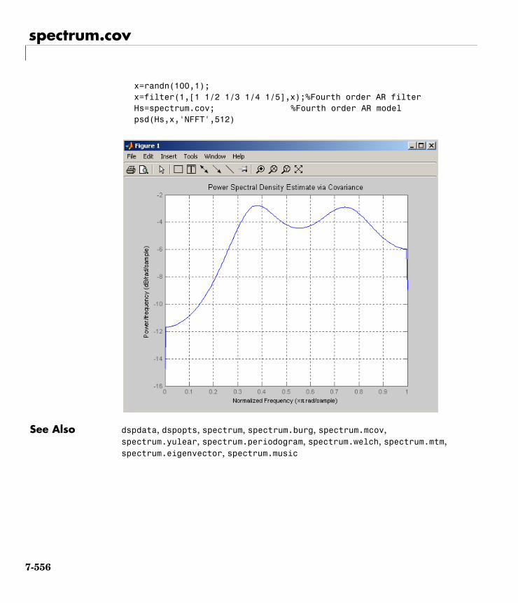
spectrum.cov
x=randn(100,1);x=filter(1,[1 1/2 1/3 1/4 1/5],x);%Fourth order AR filterHs=spectrum.cov; %Fourth order AR modelpsd(Hs,x,'NFFT',512)
See Also dspdata, dspopts, spectrum, spectrum.burg, spectrum.mcov, spectrum.yulear, spectrum.periodogram, spectrum.welch, spectrum.mtm, spectrum.eigenvector, spectrum.music
7-556
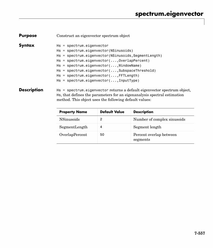
spectrum.eigenvector
7spectrum.eigenvectorPurpose Construct an eigenvector spectrum object
Syntax Hs = spectrum.eigenvectorHs = spectrum.eigenvector(NSinusoids)Hs = spectrum.eigenvector(NSinusoids,SegmentLength)Hs = spectrum.eigenvector(...,OverlapPercent)Hs = spectrum.eigenvector(...,WindowName)Hs = spectrum.eigenvector(...,SubspaceThreshold)Hs = spectrum.eigenvector(...,FFTLength)Hs = spectrum.eigenvector(...,InputType)
Description Hs = spectrum.eigenvector returns a default eigenvector spectrum object, Hs, that defines the parameters for an eigenanalysis spectral estimation method. This object uses the following default values:
Property Name Default Value Description
NSinusoids 2 Number of complex sinusoids
SegmentLength 4 Segment length
OverlapPercent 50 Percent overlap between segments
7-557
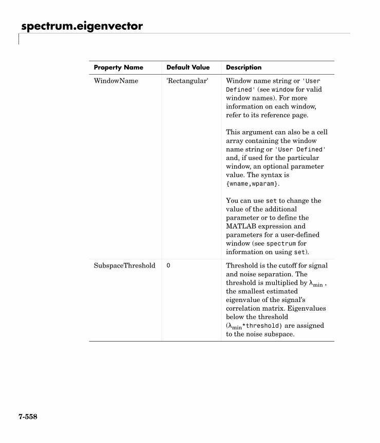
spectrum.eigenvector
WindowName 'Rectangular' Window name string or 'User Defined' (see window for valid window names). For more information on each window, refer to its reference page.
This argument can also be a cell array containing the window name string or 'User Defined' and, if used for the particular window, an optional parameter value. The syntax is wname,wparam.
You can use set to change the value of the additional parameter or to define the MATLAB expression and parameters for a user-defined window (see spectrum for information on using set).
SubspaceThreshold 0 Threshold is the cutoff for signal and noise separation. The threshold is multiplied by λmin , the smallest estimated eigenvalue of the signal’s correlation matrix. Eigenvalues below the threshold (λmin*threshold) are assigned to the noise subspace.
Property Name Default Value Description
7-558
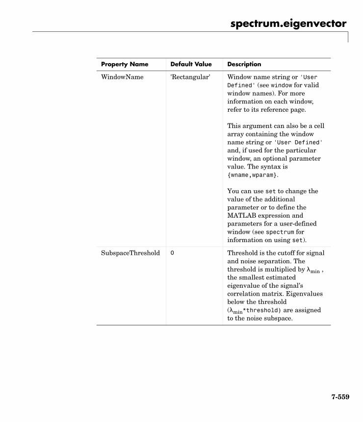
spectrum.eigenvector
WindowName 'Rectangular' Window name string or 'User Defined' (see window for valid window names). For more information on each window, refer to its reference page.
This argument can also be a cell array containing the window name string or 'User Defined' and, if used for the particular window, an optional parameter value. The syntax is wname,wparam.
You can use set to change the value of the additional parameter or to define the MATLAB expression and parameters for a user-defined window (see spectrum for information on using set).
SubspaceThreshold 0 Threshold is the cutoff for signal and noise separation. The threshold is multiplied by λmin , the smallest estimated eigenvalue of the signal’s correlation matrix. Eigenvalues below the threshold (λmin*threshold) are assigned to the noise subspace.
Property Name Default Value Description
7-559
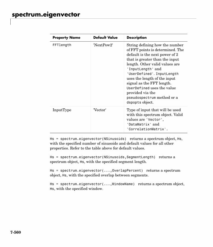
spectrum.eigenvector
Hs = spectrum.eigenvector(NSinusoids) returns a spectrum object, Hs, with the specified number of sinusoids and default values for all other properties. Refer to the table above for default values.
Hs = spectrum.eigenvector(NSinusoids,SegmentLength) returns a spectrum object, Hs, with the specified segment length.
Hs = spectrum.eigenvector(...,OverlapPercent) returns a spectrum object, Hs, with the specified overlap between segments.
Hs = spectrum.eigenvector(...,WindowName) returns a spectrum object, Hs, with the specified window.
FFTlength 'NextPow2' String defining how the number of FFT points is determined. The default is the next power of 2 that is greater than the input length. Other valid values are 'InputLength' and 'UserDefined'. InputLength uses the length of the input signal as the FFT length. UserDefined uses the value provided via the pseudospectrum method or a dspopts object.
InputType 'Vector' Type of input that will be used with this spectrum object. Valid values are 'Vector', 'DataMatrix' and 'CorrelationMatrix'.
Property Name Default Value Description
7-560
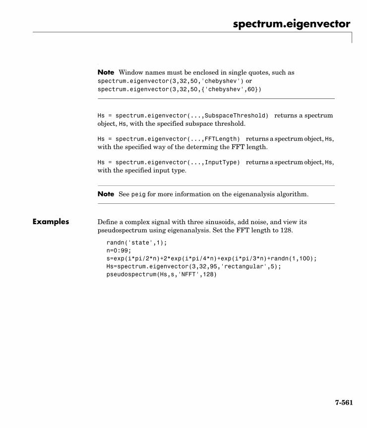
spectrum.eigenvector
Note Window names must be enclosed in single quotes, such as spectrum.eigenvector(3,32,50,'chebyshev') or spectrum.eigenvector(3,32,50,'chebyshev',60)
Hs = spectrum.eigenvector(...,SubspaceThreshold) returns a spectrum object, Hs, with the specified subspace threshold.
Hs = spectrum.eigenvector(...,FFTLength) returns a spectrum object, Hs, with the specified way of the determing the FFT length.
Hs = spectrum.eigenvector(...,InputType) returns a spectrum object, Hs, with the specified input type.
Note See peig for more information on the eigenanalysis algorithm.
Examples Define a complex signal with three sinusoids, add noise, and view its pseudospectrum using eigenanalysis. Set the FFT length to 128.
randn('state',1);n=0:99;s=exp(i*pi/2*n)+2*exp(i*pi/4*n)+exp(i*pi/3*n)+randn(1,100);Hs=spectrum.eigenvector(3,32,95,'rectangular',5);pseudospectrum(Hs,s,'NFFT',128)
7-561
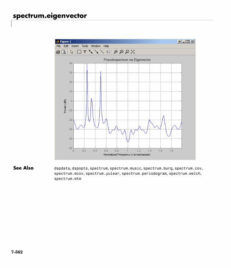
spectrum.eigenvector
See Also dspdata, dspopts, spectrum, spectrum.music, spectrum.burg, spectrum.cov, spectrum.mcov, spectrum.yulear, spectrum.periodogram, spectrum.welch, spectrum.mtm
7-562
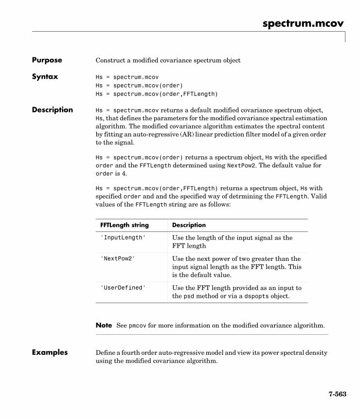
spectrum.mcov
7spectrum.mcovPurpose Construct a modified covariance spectrum object
Syntax Hs = spectrum.mcovHs = spectrum.mcov(order)Hs = spectrum.mcov(order,FFTLength)
Description Hs = spectrum.mcov returns a default modified covariance spectrum object, Hs, that defines the parameters for the modified covariance spectral estimation algorithm. The modified covariance algorithm estimates the spectral content by fitting an auto-regressive (AR) linear prediction filter model of a given order to the signal.
Hs = spectrum.mcov(order) returns a spectrum object, Hs with the specified order and the FFTLength determined using NextPow2. The default value for order is 4.
Hs = spectrum.mcov(order,FFTLength) returns a spectrum object, Hs with specified order and and the specified way of detrmining the FFTLength. Valid values of the FFTLength string are as follows:
Note See pmcov for more information on the modified covariance algorithm.
Examples Define a fourth order auto-regressive model and view its power spectral density using the modified covariance algorithm.
FFTLength string Description
'InputLength' Use the length of the input signal as the FFT length
'NextPow2' Use the next power of two greater than the input signal length as the FFT length. This is the default value.
'UserDefined' Use the FFT length provided as an input to the psd method or via a dspopts object.
7-563
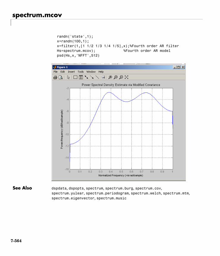
spectrum.mcov
randn('state',1);x=randn(100,1);x=filter(1,[1 1/2 1/3 1/4 1/5],x);%Fourth order AR filterHs=spectrum.mcov); %Fourth order AR modelpsd(Hs,x,'NFFT',512)
See Also dspdata, dspopts, spectrum, spectrum.burg, spectrum.cov, spectrum.yulear, spectrum.periodogram, spectrum.welch, spectrum.mtm, spectrum.eigenvector, spectrum.music
7-564
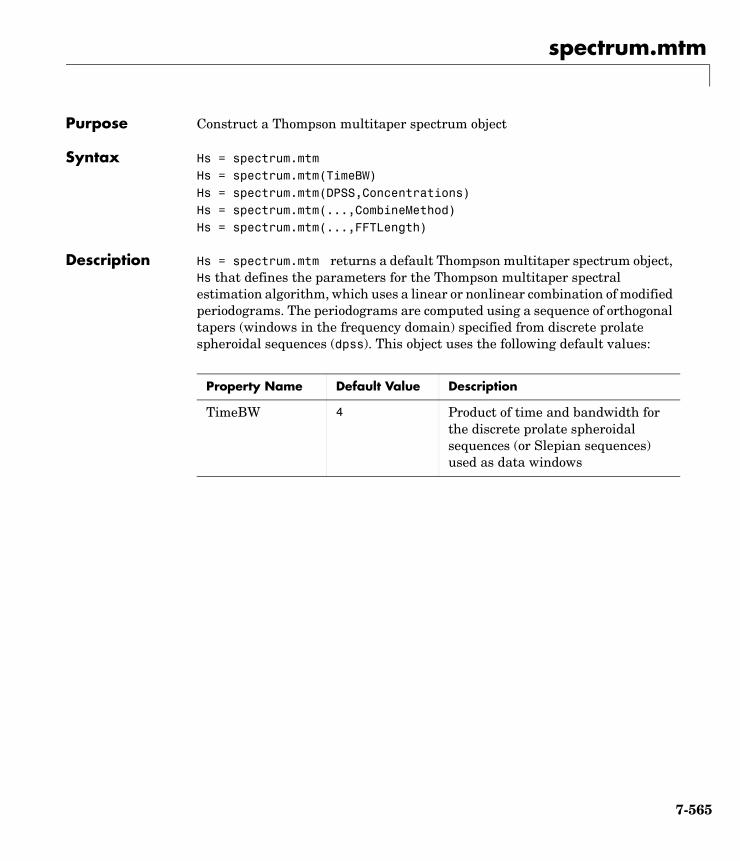
spectrum.mtm
7spectrum.mtmPurpose Construct a Thompson multitaper spectrum object
Syntax Hs = spectrum.mtmHs = spectrum.mtm(TimeBW)Hs = spectrum.mtm(DPSS,Concentrations)Hs = spectrum.mtm(...,CombineMethod)Hs = spectrum.mtm(...,FFTLength)
Description Hs = spectrum.mtm returns a default Thompson multitaper spectrum object, Hs that defines the parameters for the Thompson multitaper spectral estimation algorithm, which uses a linear or nonlinear combination of modified periodograms. The periodograms are computed using a sequence of orthogonal tapers (windows in the frequency domain) specified from discrete prolate spheroidal sequences (dpss). This object uses the following default values:
Property Name Default Value Description
TimeBW 4 Product of time and bandwidth for the discrete prolate spheroidal sequences (or Slepian sequences) used as data windows
7-565
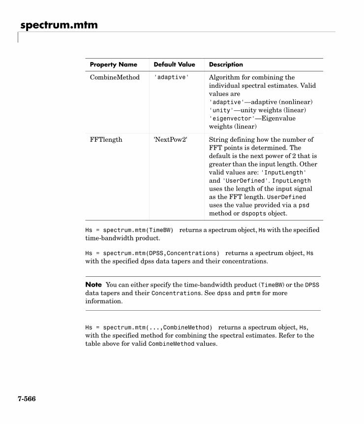
spectrum.mtm
Hs = spectrum.mtm(TimeBW) returns a spectrum object, Hs with the specified time-bandwidth product.
Hs = spectrum.mtm(DPSS,Concentrations) returns a spectrum object, Hs with the specified dpss data tapers and their concentrations.
Note You can either specify the time-bandwidth product (TimeBW) or the DPSS data tapers and their Concentrations. See dpss and pmtm for more information.
Hs = spectrum.mtm(...,CombineMethod) returns a spectrum object, Hs, with the specified method for combining the spectral estimates. Refer to the table above for valid CombineMethod values.
CombineMethod 'adaptive' Algorithm for combining the individual spectral estimates. Valid values are 'adaptive'—adaptive (nonlinear)'unity'—unity weights (linear)'eigenvector'—Eigenvalue weights (linear)
FFTlength 'NextPow2' String defining how the number of FFT points is determined. The default is the next power of 2 that is greater than the input length. Other valid values are: 'InputLength' and 'UserDefined'. InputLength uses the length of the input signal as the FFT length. UserDefined uses the value provided via a psd method or dspopts object.
Property Name Default Value Description
7-566
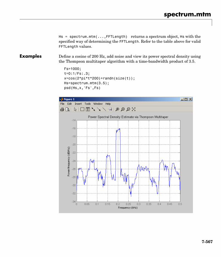
spectrum.mtm
Hs = spectrum.mtm(...,FFTLength) returns a spectrum object, Hs with the specified way of determining the FFTLength. Refer to the table above for valid FFTLength values.
Examples Define a cosine of 200 Hz, add noise and view its power spectral density using the Thompson multitaper algorithm with a time-bandwidth product of 3.5.
Fs=1000;t=0:1/Fs:.3;x=cos(2*pi*t*200)+randn(size(t));Hs=spectrum.mtm(3.5);psd(Hs,x,'Fs',Fs)
7-567

spectrum.mtm
The above example could be done by specifying the data tapers and concentrations instead of the time-bandwidth product.
Fs=1000;t=0:1/Fs:.3;x=cos(2*pi*t*200)+randn(size(t));[e,v]=dpss(length(x),3.5);Hs=spectrum.mtm(e,v);psd(Hs,x,Fs)
See Also dspdata, dspopts, spectrum, spectrum.periodogram, spectrum.welch, spectrum.burg, spectrum.cov, spectrum.mcov, spectrum.yulear, spectrum.eigenvector, spectrum.music
7-568
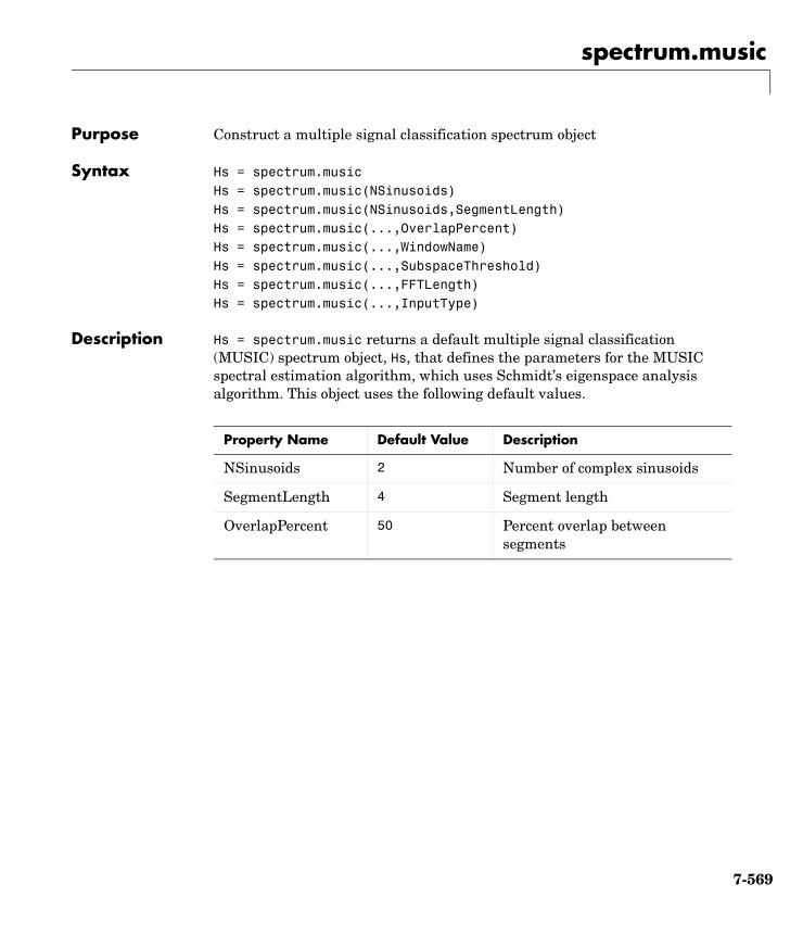
spectrum.music
7spectrum.musicPurpose Construct a multiple signal classification spectrum object
Syntax Hs = spectrum.musicHs = spectrum.music(NSinusoids)Hs = spectrum.music(NSinusoids,SegmentLength)Hs = spectrum.music(...,OverlapPercent)Hs = spectrum.music(...,WindowName)Hs = spectrum.music(...,SubspaceThreshold)Hs = spectrum.music(...,FFTLength)Hs = spectrum.music(...,InputType)
Description Hs = spectrum.music returns a default multiple signal classification (MUSIC) spectrum object, Hs, that defines the parameters for the MUSIC spectral estimation algorithm, which uses Schmidt’s eigenspace analysis algorithm. This object uses the following default values.
Property Name Default Value Description
NSinusoids 2 Number of complex sinusoids
SegmentLength 4 Segment length
OverlapPercent 50 Percent overlap between segments
7-569
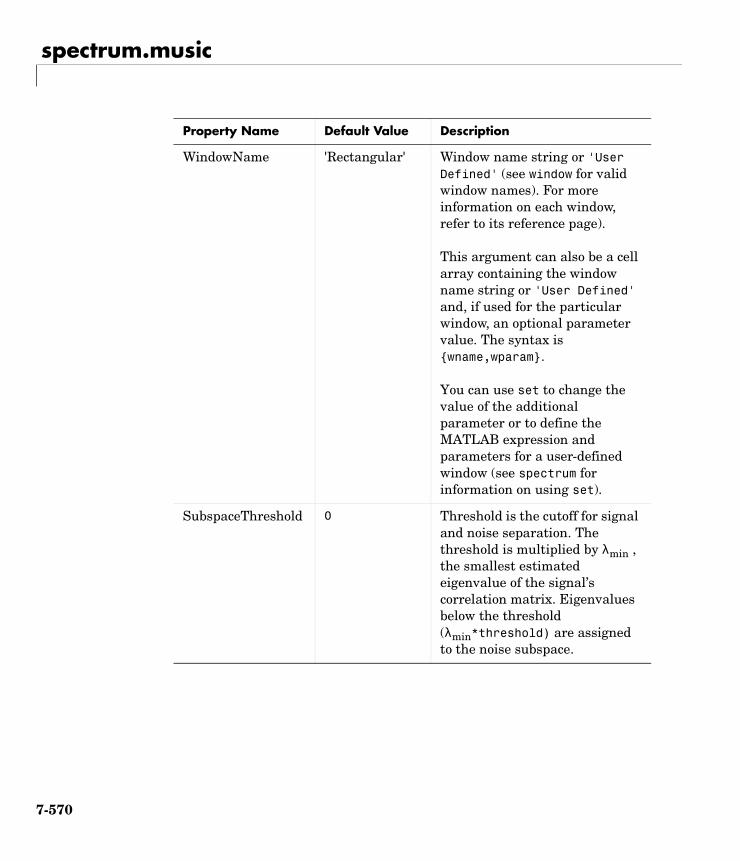
spectrum.music
WindowName 'Rectangular' Window name string or 'User Defined' (see window for valid window names). For more information on each window, refer to its reference page).
This argument can also be a cell array containing the window name string or 'User Defined' and, if used for the particular window, an optional parameter value. The syntax is wname,wparam.
You can use set to change the value of the additional parameter or to define the MATLAB expression and parameters for a user-defined window (see spectrum for information on using set).
SubspaceThreshold 0 Threshold is the cutoff for signal and noise separation. The threshold is multiplied by λmin , the smallest estimated eigenvalue of the signal’s correlation matrix. Eigenvalues below the threshold (λmin*threshold) are assigned to the noise subspace.
Property Name Default Value Description
7-570
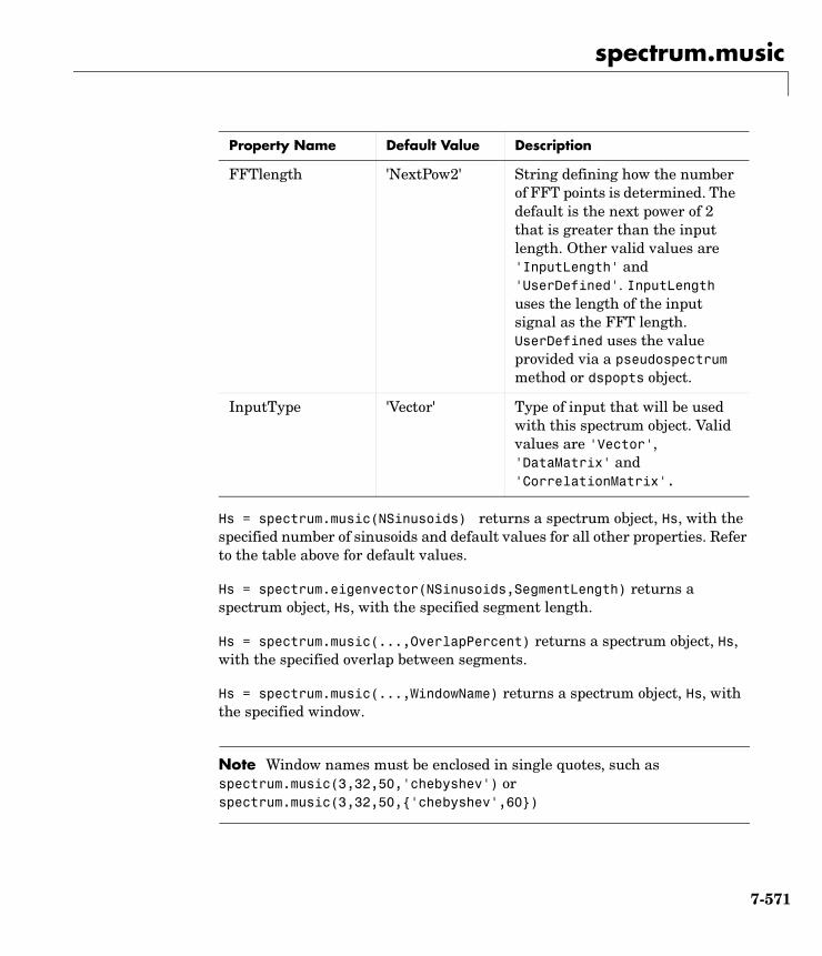
spectrum.music
Hs = spectrum.music(NSinusoids) returns a spectrum object, Hs, with the specified number of sinusoids and default values for all other properties. Refer to the table above for default values.
Hs = spectrum.eigenvector(NSinusoids,SegmentLength) returns a spectrum object, Hs, with the specified segment length.
Hs = spectrum.music(...,OverlapPercent) returns a spectrum object, Hs, with the specified overlap between segments.
Hs = spectrum.music(...,WindowName) returns a spectrum object, Hs, with the specified window.
Note Window names must be enclosed in single quotes, such as spectrum.music(3,32,50,'chebyshev') or spectrum.music(3,32,50,'chebyshev',60)
FFTlength 'NextPow2' String defining how the number of FFT points is determined. The default is the next power of 2 that is greater than the input length. Other valid values are 'InputLength' and 'UserDefined'. InputLength uses the length of the input signal as the FFT length. UserDefined uses the value provided via a pseudospectrum method or dspopts object.
InputType 'Vector' Type of input that will be used with this spectrum object. Valid values are 'Vector', 'DataMatrix' and 'CorrelationMatrix'.
Property Name Default Value Description
7-571

spectrum.music
Hs = spectrum.music(...,SubspaceThreshold) returns a spectrum object, Hs, with the specified subspace threshold.
Hs = spectrum.music(...,FFTLength) returns a spectrum object, Hs, with the specified FFT length type.
Hs = spectrum.music(...,InputType) returns a spectrum object, Hs, with the specified input type.
Note See pmusic for more information on the MUSIC algorithm.
Examples Define a complex signal with three sinusoids, add noise, and estimate its pseudospectrum using the MUSIC algorithm.
randn('state',1);n=0:99;s=exp(i*pi/2*n)+2*exp(i*pi/4*n)+exp(i*pi/3*n)+randn(1,100);Hs=spectrum.music(3);pseudospectrum(Hs,s,'NFFT',512)
7-572
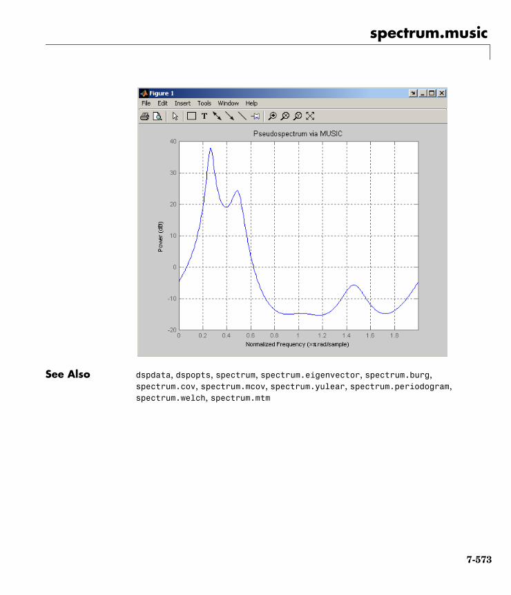
spectrum.music
See Also dspdata, dspopts, spectrum, spectrum.eigenvector, spectrum.burg, spectrum.cov, spectrum.mcov, spectrum.yulear, spectrum.periodogram, spectrum.welch, spectrum.mtm
7-573
spectrum.periodogram
7spectrum.periodogramPurpose Construct a periodogram spectrum object
Syntax Hs = spectrum.periodogramHs = spectrum.periodogram(winname)Hs = spectrum.periodogram(winname,winparameter)Hs = spectrum.periodogram(...,FFTLength)
Description Hs = spectrum.periodogram returns a default periodogram spectrum object, Hs, that defines the parameters for theperiodogram spectral estimation method. This default object uses a rectangular window and a default FFT length equal to the next power of 2 (NextPow2) that is greater than the input length.
Hs = spectrum.periodogram(winname) returns a spectrum object, Hs, that uses the specified window. If the window uses an optional associated window parameter, it is set to the default value. This object uses the default FFT length.
Hs = spectrum.periodogram(winname,winparameter) returns a spectrum object, Hs, that uses the specified window and optional associated window parameter, if any. You specify the window and window parameter in a cell array with a windowname string and the parameter value. This object uses the default FFT length.
Valid windowname strings are any valid window in the Signal Processing Toolbox or a user-defined window. Refer to the corresponding window function page for window parameter information.
You can use set to change the value of the additional parameter or to define the MATLAB expression and parameters for a user-defined window (see spectrum for information on using set).
Note Window names must be enclosed in single quotes, such as spectrum.periodogram('tukey') orspectrum.periodogram('tukey',0.7)
7-574
spectrum.periodogram
Hs = spectrum.periodogram(...,FFTLength) returns a spectrum object, Hs that uses the specified way of determining the FFTLength. Valid values of the FFTLength string are as follows.
Note See periodogram for more information on the periodogram algorithm.
Examples Define a cosine of 200 Hz, add noise and view its spectral content using the periodogram spectral estimation technique.
Fs=1000;t=0:1/Fs:.3;x=cos(2*pi*t*200)+randn(size(t));Hs=spectrum.periodogram; % Use default valuespsd(Hs,x,'Fs',Fs)
FFTLength string Description
'InputLength' Use the length of the input signal as the FFT length
'NextPow2' Use the next power of two greater than the input signal length as the FFT length. This is the default value.
'UserDefined' Use the FFT length provided as an input to the psd method or via a dspopts object.
7-575
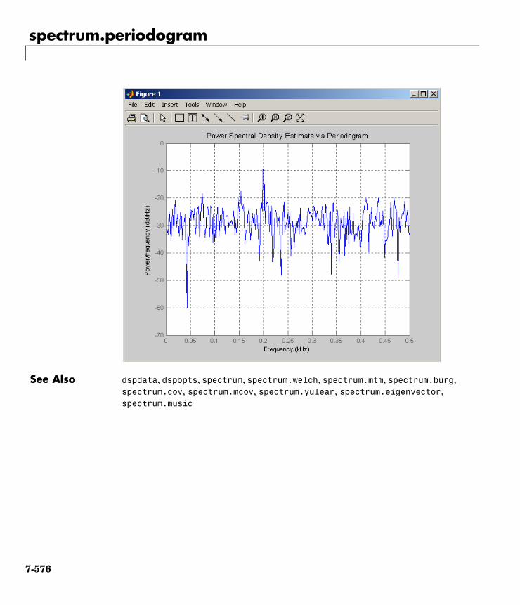
spectrum.periodogram
See Also dspdata, dspopts, spectrum, spectrum.welch, spectrum.mtm, spectrum.burg, spectrum.cov, spectrum.mcov, spectrum.yulear, spectrum.eigenvector, spectrum.music
7-576
spectrum.welch
7spectrum.welchPurpose Construct a Welch spectrum object
Syntax Hs = spectrum.welchHs = spectrum.welch(WindowName)Hs = spectrum.welch(WindowName,winparam)Hs = spectrum.welch(...,SegmentLength)Hs = spectrum.welch(...,OverlapPercent)Hs = spectrum.welch(...,FFTLength)
Description Hs = spectrum.welch returns a default Welch spectrum object, Hs, that defines the parameters for Welch’s averaged, modified periodogram spectral estimation method. The object uses these default values.
Property Name Default Value Description
WindowName 'Hamming',SamplingFlag: symmetric
Window name string or 'User Defined' (see window for valid window names). If the window uses an optional property, it is set to the default value.
WindowName,winparam
Cell array containing WindowName and optional window parameter
'Hamming',SamplingFlag: symmetric
Cell array containing the window name string or 'User Defined' and, if used for the particular window, an optional parameter value. (See window for valid window names and for more information on each window, refer to its reference page.)
You can use set to change the value of the additional parameter or to define the MATLAB expression and parameters for a user-defined window. (See spectrum for information on using set.)
7-577
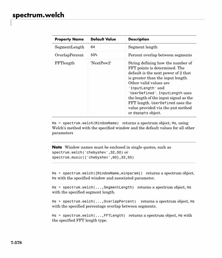
spectrum.welch
Hs = spectrum.welch(WindowName) returns a spectrum object, Hs, using Welch’s method with the specified window and the default values for all other parameters
Note Window names must be enclosed in single quotes, such as spectrum.welch('chebyshev',32,50) or spectrum.music('chebyshev',60,32,50)
Hs = spectrum.welch(WindowName,winparam) returns a spectrum object, Hs with the specified window and associated parameter.
Hs = spectrum.welch(...,SegmentLength) returns a spectrum object, Hs with the specified segment length.
Hs = spectrum.welch(...,OverlapPercent) returns a spectrum object, Hs with the specified percentage overlap between segments.
Hs = spectrum.welch(...,FFTLength) returns a spectrum object, Hs with the specified FFT length type.
SegmentLength 64 Segment length
OverlapPercent 50% Percent overlap between segments
FFTlength 'NextPow2' String defining how the number of FFT points is determined. The default is the next power of 2 that is greater than the input length. Other valid values are 'InputLength' and 'UserDefined'. InputLength uses the length of the input signal as the FFT length. UserDefined uses the value provided via the psd method or dspopts object.
Property Name Default Value Description
7-578
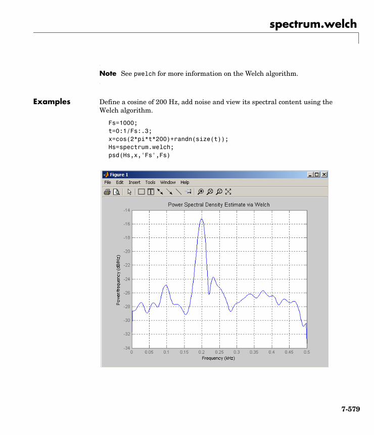
spectrum.welch
Note See pwelch for more information on the Welch algorithm.
Examples Define a cosine of 200 Hz, add noise and view its spectral content using the Welch algorithm.
Fs=1000;t=0:1/Fs:.3;x=cos(2*pi*t*200)+randn(size(t));Hs=spectrum.welch;psd(Hs,x,'Fs',Fs)
7-579

spectrum.welch
See Also dspdata, dspopts, spectrum, spectrum.periodogram, spectrum.mtm, spectrum.burg, spectrum.cov, spectrum.mcov, spectrum.yulear, spectrum.eigenvector, spectrum.music
7-580
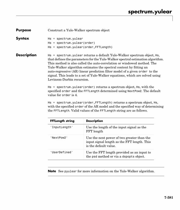
spectrum.yulear
7spectrum.yulearPurpose Construct a Yule-Walker spectrum object
Syntax Hs = spectrum.yulearHs = spectrum.yulear(order)Hs = spectrum.yulear(order,FFTLength)
Description Hs = spectrum.yulear returns a default Yule-Walker spectrum object, Hs, that defines the parameters for the Yule-Walker spectral estimation algorithm. This method is also called the auto-correlation or windowed method. The Yule-Walker algorithm estimates the spectral content by fitting an auto-regressive (AR) linear prediction filter model of a given order to the signal. This leads to a set of Yule-Walker equations, which are solved using Levinson-Durbin recursion.
Hs = spectrum.yulear(order) returns a spectrum object, Hs, with the specified order and the FFTLength determined using NextPow2. The default value for order is 4.
Hs = spectrum.yulear(order,FFTLength) returns a spectrum object, Hs, with the specified order of the AR model and the specified way of determining the FFTLength. Valid values of the FFTLength string are as follows.
Note See pyulear for more information on the Yule-Walker algorithm.
FFTLength string Description
'InputLength' Use the length of the input signal as the FFT length
'NextPow2' Use the next power of two greater than the input signal length as the FFT length. This is the default value.
'UserDefined' Use the FFT length provided as an input to the psd method or via a dspopts object.
7-581
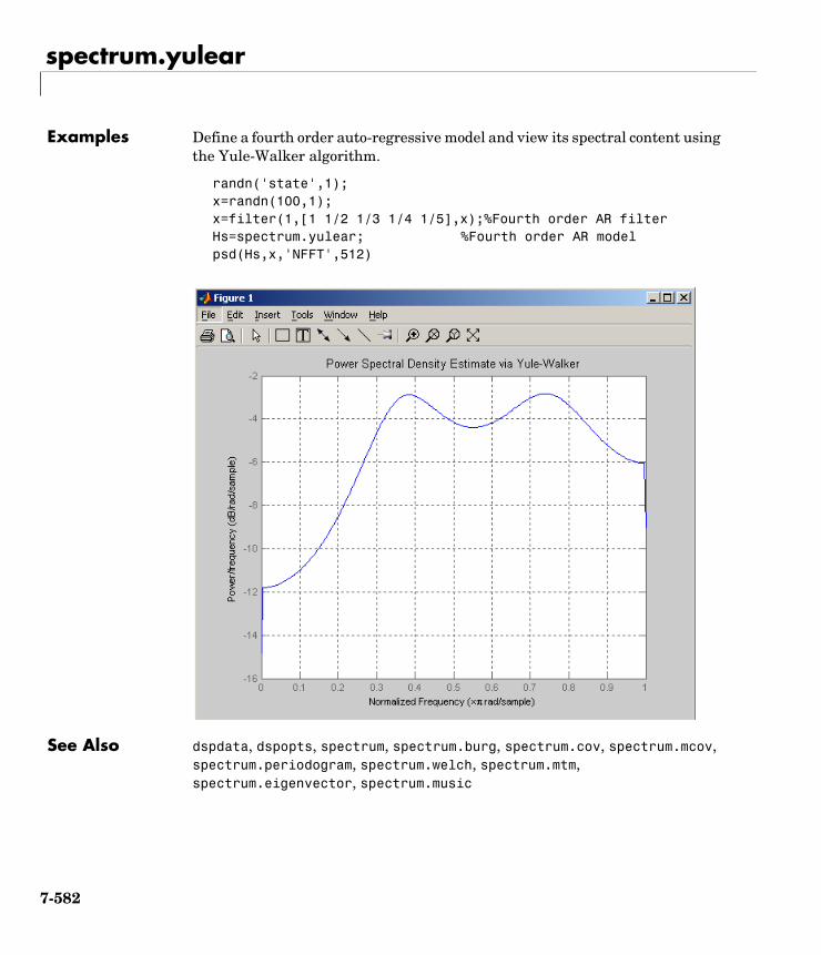
spectrum.yulear
Examples Define a fourth order auto-regressive model and view its spectral content using the Yule-Walker algorithm.
randn('state',1);x=randn(100,1);x=filter(1,[1 1/2 1/3 1/4 1/5],x);%Fourth order AR filterHs=spectrum.yulear; %Fourth order AR modelpsd(Hs,x,'NFFT',512)
See Also dspdata, dspopts, spectrum, spectrum.burg, spectrum.cov, spectrum.mcov, spectrum.periodogram, spectrum.welch, spectrum.mtm, spectrum.eigenvector, spectrum.music
7-582
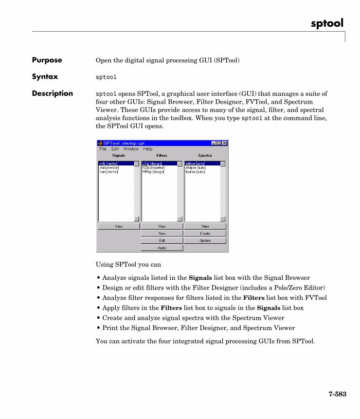
sptool
7sptoolPurpose Open the digital signal processing GUI (SPTool)
Syntax sptool
Description sptool opens SPTool, a graphical user interface (GUI) that manages a suite of four other GUIs: Signal Browser, Filter Designer, FVTool, and Spectrum Viewer. These GUIs provide access to many of the signal, filter, and spectral analysis functions in the toolbox. When you type sptool at the command line, the SPTool GUI opens.
Using SPTool you can
• Analyze signals listed in the Signals list box with the Signal Browser
• Design or edit filters with the Filter Designer (includes a Pole/Zero Editor)
• Analyze filter responses for filters listed in the Filters list box with FVTool
• Apply filters in the Filters list box to signals in the Signals list box
• Create and analyze signal spectra with the Spectrum Viewer
• Print the Signal Browser, Filter Designer, and Spectrum Viewer
You can activate the four integrated signal processing GUIs from SPTool.
7-583
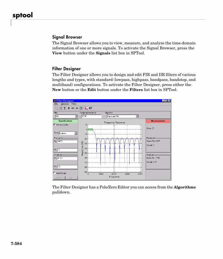
sptool
Signal BrowserThe Signal Browser allows you to view, measure, and analyze the time-domain information of one or more signals. To activate the Signal Browser, press the View button under the Signals list box in SPTool.
Filter DesignerThe Filter Designer allows you to design and edit FIR and IIR filters of various lengths and types, with standard (lowpass, highpass, bandpass, bandstop, and multiband) configurations. To activate the Filter Designer, press either the New button or the Edit button under the Filters list box in SPTool.
The Filter Designer has a Pole/Zero Editor you can access from the Algorithms pulldown.
7-584
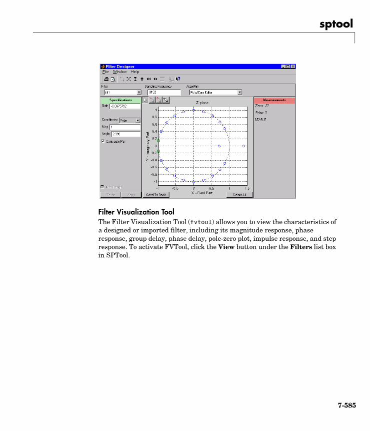
sptool
Filter Visualization ToolThe Filter Visualization Tool (fvtool) allows you to view the characteristics of a designed or imported filter, including its magnitude response, phase response, group delay, phase delay, pole-zero plot, impulse response, and step response. To activate FVTool, click the View button under the Filters list box in SPTool.
7-585
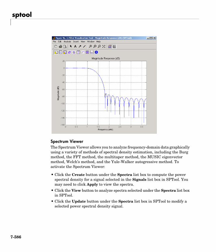
sptool
Spectrum ViewerThe Spectrum Viewer allows you to analyze frequency-domain data graphically using a variety of methods of spectral density estimation, including the Burg method, the FFT method, the multitaper method, the MUSIC eigenvector method, Welch’s method, and the Yule-Walker autogressive method. To activate the Spectrum Viewer:
• Click the Create button under the Spectra list box to compute the power spectral density for a signal selected in the Signals list box in SPTool. You may need to click Apply to view the spectra.
• Click the View button to analyze spectra selected under the Spectra list box in SPTool.
• Click the Update button under the Spectra list box in SPTool to modify a selected power spectral density signal.
7-586
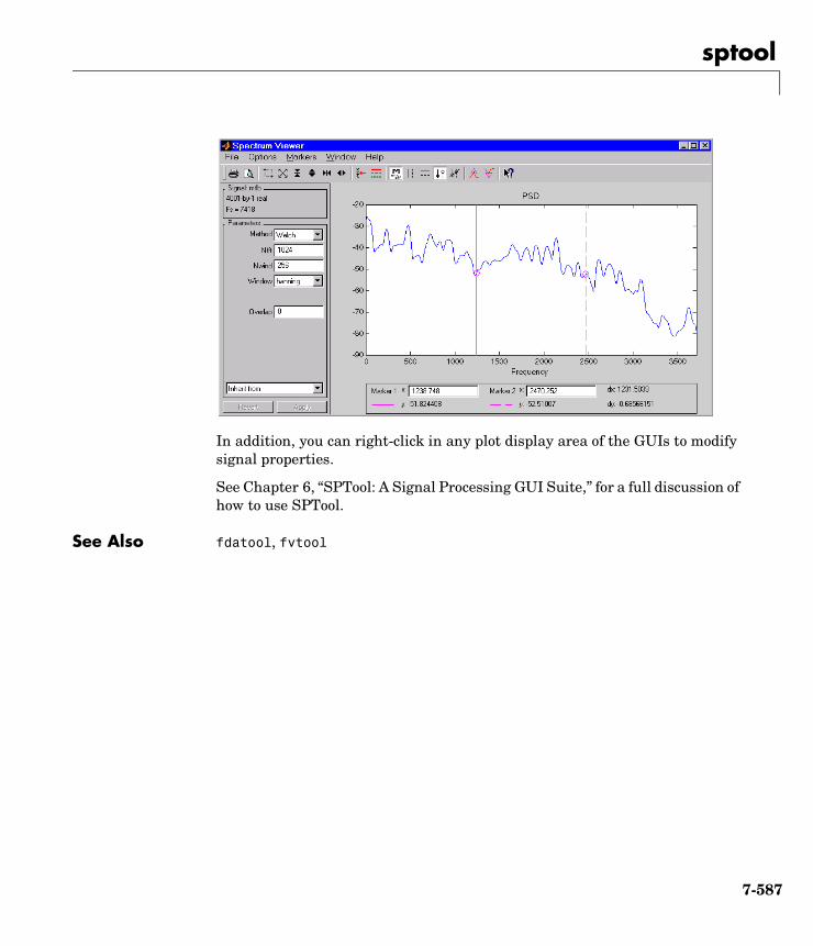
sptool
In addition, you can right-click in any plot display area of the GUIs to modify signal properties.
See Chapter 6, “SPTool: A Signal Processing GUI Suite,” for a full discussion of how to use SPTool.
See Also fdatool, fvtool
7-587
square
7squarePurpose Generate a square wave
Syntax x = square(t)x = square(t,duty)
Description x = square(t) generates a square wave with period 2π for the elements of time vector t. square(t) is similar to sin(t), but creates a square wave with peaks of ±1 instead of a sine wave.
x = square(t,duty) generates a square wave with specified duty cycle, duty, which is a number between 0 and 100. The duty cycle is the percent of the period in which the signal is positive.
See Also chirp, cos, diric, gauspuls, pulstran, rectpuls, sawtooth, sin, square, tripuls
7-588
ss2sos
7ss2sosPurpose Convert digital filter state-space parameters to second-order sections form
Syntax [sos,g] = ss2sos(A,B,C,D)[sos,g] = ss2sos(A,B,C,D,iu)[sos,g] = ss2sos(A,B,C,D,'order')[sos,g] = ss2sos(A,B,C,D,iu,'order')[sos,g] = ss2sos(A,B,C,D,iu,'order','scale')sos = ss2sos(...)
Description ss2sos converts a state-space representation of a given digital filter to an equivalent second-order section representation.
[sos,g] = ss2sos(A,B,C,D) finds a matrix sos in second-order section form with gain g that is equivalent to the state-space system represented by input arguments A, B, C, and D. The input system must be single output and real. sos is an L-by-6 matrix
whose rows contain the numerator and denominator coefficients bik and aik of the second-order sections of H(z).
[sos,g] = ss2sos(A,B,C,D,iu) specifies a scalar iu that determines which input of the state-space system A, B, C, D is used in the conversion. The default for iu is 1.
[sos,g] = ss2sos(A,B,C,D,'order') and
[sos,g] = ss2sos(A,B,C,D,iu,'order') specify the order of the rows in sos, where 'order' is
sos
b01 b11 b21 1 a11 a21
b02 b12 b22 1 a12 a22
b0L b1L b2L 1 a1L a2L
=
H z( ) g Hk z( )
k 1=
L
∏ gb0k b1kz 1– b2kz 2–+ +
1 a1kz 1– a2kz 2–+ +----------------------------------------------------------
k 1=
L
∏= =
7-589
ss2sos
• 'down', to order the sections so the first row of sos contains the poles closest to the unit circle
• 'up', to order the sections so the first row of sos contains the poles farthest from the unit circle (default)
The zeros are always paired with the poles closest to them.
[sos,g] = ss2sos(A,B,C,D,iu,'order','scale') specifies the desired scaling of the gain and the numerator coefficients of all second-order sections, where 'scale' is
• 'none', to apply no scaling (default)
• 'inf', to apply infinity-norm scaling
• 'two', to apply 2-norm scaling
Using infinity-norm scaling in conjunction with up-ordering minimizes the probability of overflow in the realization. Using 2-norm scaling in conjunction with down-ordering minimizes the peak round-off noise.
Note Infinity-norm and 2-norm scaling are appropriate only for direct-form II implementations.
sos = ss2sos(...) embeds the overall system gain, g, in the first section, H1(z), so that
Note Embedding the gain in the first section when scaling a direct-form II structure is not recommended and may result in erratic scaling. To avoid embedding the gain, use ss2sos with two outputs.
Examples Find a second-order section form of a Butterworth lowpass filter:
H z( ) Hk z( )
k 1=
L
∏=
7-590
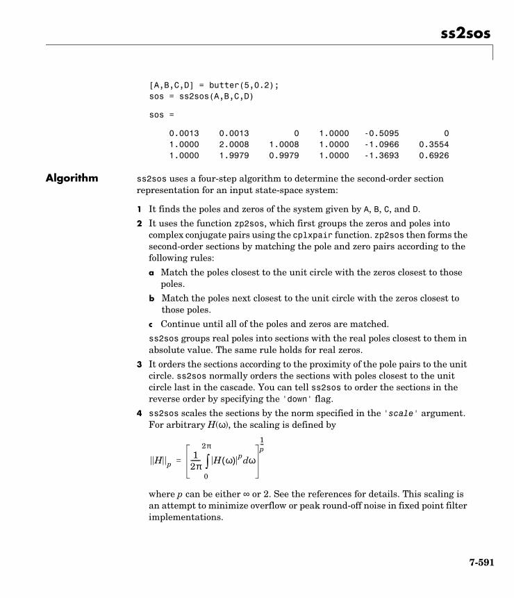
ss2sos
[A,B,C,D] = butter(5,0.2);sos = ss2sos(A,B,C,D)
sos =
0.0013 0.0013 0 1.0000 -0.5095 0 1.0000 2.0008 1.0008 1.0000 -1.0966 0.3554 1.0000 1.9979 0.9979 1.0000 -1.3693 0.6926
Algorithm ss2sos uses a four-step algorithm to determine the second-order section representation for an input state-space system:
1 It finds the poles and zeros of the system given by A, B, C, and D.
2 It uses the function zp2sos, which first groups the zeros and poles into complex conjugate pairs using the cplxpair function. zp2sos then forms the second-order sections by matching the pole and zero pairs according to the following rules:
a Match the poles closest to the unit circle with the zeros closest to those poles.
b Match the poles next closest to the unit circle with the zeros closest to those poles.
c Continue until all of the poles and zeros are matched.
ss2sos groups real poles into sections with the real poles closest to them in absolute value. The same rule holds for real zeros.
3 It orders the sections according to the proximity of the pole pairs to the unit circle. ss2sos normally orders the sections with poles closest to the unit circle last in the cascade. You can tell ss2sos to order the sections in the reverse order by specifying the 'down' flag.
4 ss2sos scales the sections by the norm specified in the 'scale' argument. For arbitrary H(ω), the scaling is defined by
where p can be either ∞ or 2. See the references for details. This scaling is an attempt to minimize overflow or peak round-off noise in fixed point filter implementations.
H p1
2π------ H ω( ) p ωd
0
2π
∫
1p---
=
7-591

ss2sos
Diagnostics If there is more than one input to the system, ss2sos gives the following error message:
State-space system must have only one input.
See Also cplxpair, sos2ss, ss2tf, ss2zp, tf2sos, zp2sos
References [1] Jackson, L.B., Digital Filters and Signal Processing, 3rd ed., Kluwer Academic Publishers, Boston, 1996. Chapter 11.
[2] Mitra, S.K., Digital Signal Processing: A Computer-Based Approach, McGraw-Hill, New York, 1998. Chapter 9.
[3] Vaidyanathan, P.P.,“Robust Digital Filter Structures,” Handbook for Digital Signal Processing, S.K. Mitra and J.F. Kaiser, ed., John Wiley & Sons, New York, 1993, Chapter 7.
7-592
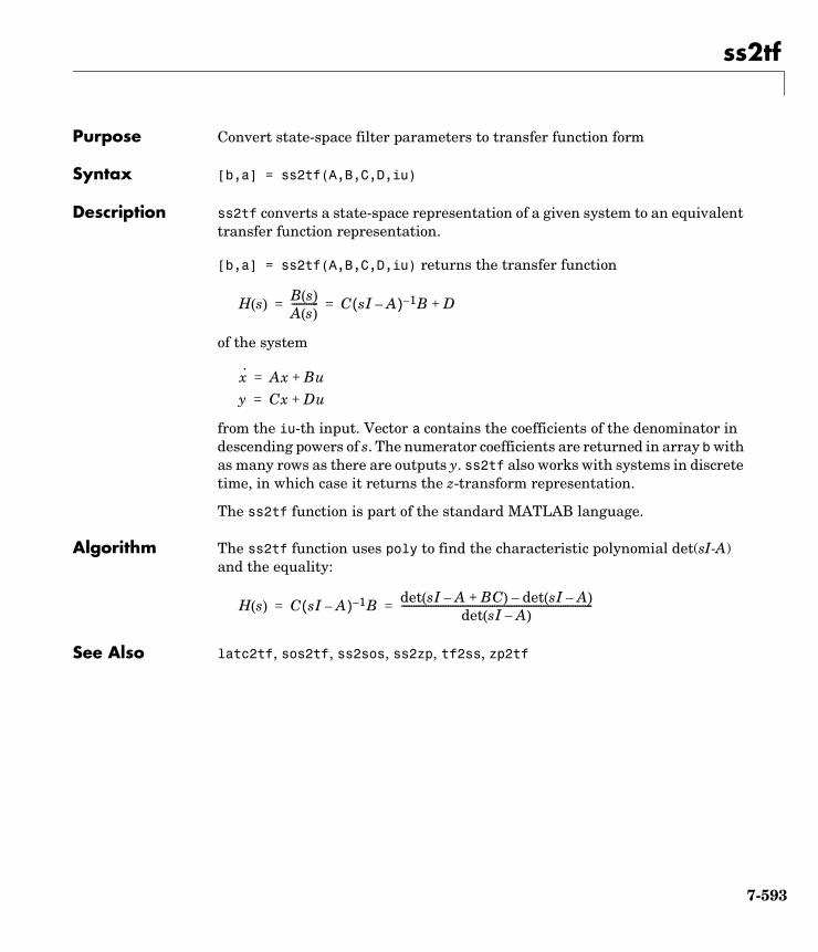
ss2tf
7ss2tfPurpose Convert state-space filter parameters to transfer function form
Syntax [b,a] = ss2tf(A,B,C,D,iu)
Description ss2tf converts a state-space representation of a given system to an equivalent transfer function representation.
[b,a] = ss2tf(A,B,C,D,iu) returns the transfer function
of the system
from the iu-th input. Vector a contains the coefficients of the denominator in descending powers of s. The numerator coefficients are returned in array b with as many rows as there are outputs y. ss2tf also works with systems in discrete time, in which case it returns the z-transform representation.
The ss2tf function is part of the standard MATLAB language.
Algorithm The ss2tf function uses poly to find the characteristic polynomial det(sI-A) and the equality:
See Also latc2tf, sos2tf, ss2sos, ss2zp, tf2ss, zp2tf
H s( )B s( )A s( )----------- C sI A–( ) 1– B D+= =
x· Ax Bu+=
y Cx Du+=
H s( ) C sI A–( ) 1– B det sI A– BC+( ) det sI A–( )–det sI A–( )
------------------------------------------------------------------------------= =
7-593
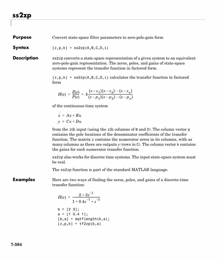
ss2zp
7ss2zpPurpose Convert state-space filter parameters to zero-pole-gain form
Syntax [z,p,k] = ss2zp(A,B,C,D,i)
Description ss2zp converts a state-space representation of a given system to an equivalent zero-pole-gain representation. The zeros, poles, and gains of state-space systems represent the transfer function in factored form.
[z,p,k] = ss2zp(A,B,C,D,i) calculates the transfer function in factored form
of the continuous-time system
from the ith input (using the ith columns of B and D). The column vector p contains the pole locations of the denominator coefficients of the transfer function. The matrix z contains the numerator zeros in its columns, with as many columns as there are outputs y (rows in C). The column vector k contains the gains for each numerator transfer function.
ss2zp also works for discrete time systems. The input state-space system must be real.
The ss2zp function is part of the standard MATLAB language.
Examples Here are two ways of finding the zeros, poles, and gains of a discrete-time transfer function:
b = [2 3]; a = [1 0.4 1];[b,a] = eqtflength(b,a);[z,p,k] = tf2zp(b,a)
H s( )Z s( )P s( )---------- k
s z1–( ) s z2–( ) s zn–( )s p1–( ) s p2–( ) s pn–( )
------------------------------------------------------------------= =
x· Ax Bu+=
y Cx Du+=
H z( )2 3z 1–
+
1 0.4z 1– z 2–+ +
-----------------------------------------=
7-594
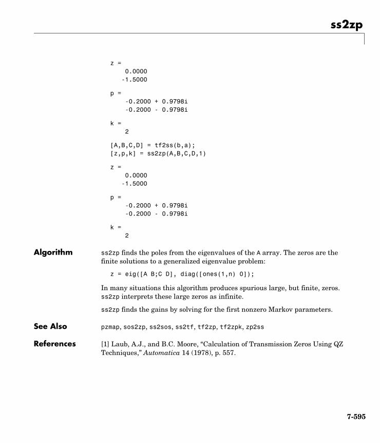
ss2zp
z = 0.0000 -1.5000
p =-0.2000 + 0.9798i-0.2000 - 0.9798i
k =2
[A,B,C,D] = tf2ss(b,a);[z,p,k] = ss2zp(A,B,C,D,1)
z = 0.0000 -1.5000
p =-0.2000 + 0.9798i-0.2000 - 0.9798i
k =2
Algorithm ss2zp finds the poles from the eigenvalues of the A array. The zeros are the finite solutions to a generalized eigenvalue problem:
z = eig([A B;C D], diag([ones(1,n) 0]);
In many situations this algorithm produces spurious large, but finite, zeros. ss2zp interprets these large zeros as infinite.
ss2zp finds the gains by solving for the first nonzero Markov parameters.
See Also pzmap, sos2zp, ss2sos, ss2tf, tf2zp, tf2zpk, zp2ss
References [1] Laub, A.J., and B.C. Moore, “Calculation of Transmission Zeros Using QZ Techniques,” Automatica 14 (1978), p. 557.
7-595
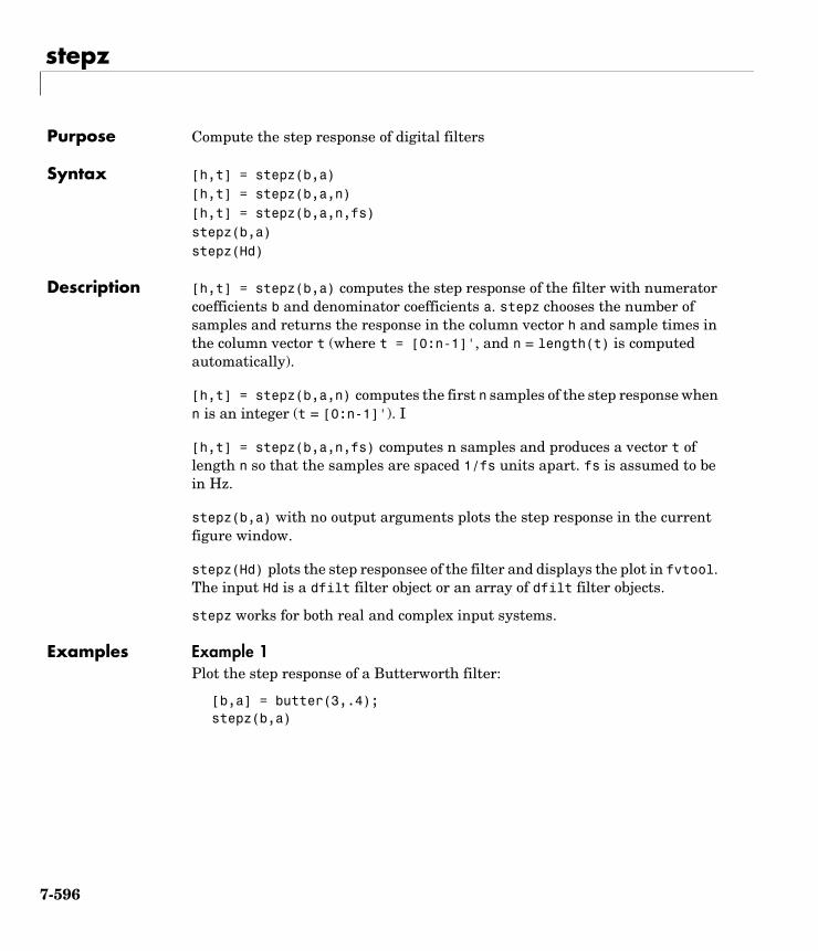
stepz
7stepzPurpose Compute the step response of digital filters
Syntax [h,t] = stepz(b,a)[h,t] = stepz(b,a,n)[h,t] = stepz(b,a,n,fs)stepz(b,a)stepz(Hd)
Description [h,t] = stepz(b,a) computes the step response of the filter with numerator coefficients b and denominator coefficients a. stepz chooses the number of samples and returns the response in the column vector h and sample times in the column vector t (where t = [0:n-1]', and n = length(t) is computed automatically).
[h,t] = stepz(b,a,n) computes the first n samples of the step response when n is an integer (t = [0:n-1]'). I
[h,t] = stepz(b,a,n,fs) computes n samples and produces a vector t of length n so that the samples are spaced 1/fs units apart. fs is assumed to be in Hz.
stepz(b,a) with no output arguments plots the step response in the current figure window.
stepz(Hd) plots the step responsee of the filter and displays the plot in fvtool. The input Hd is a dfilt filter object or an array of dfilt filter objects.
stepz works for both real and complex input systems.
Examples Example 1Plot the step response of a Butterworth filter:
[b,a] = butter(3,.4);stepz(b,a)
7-596
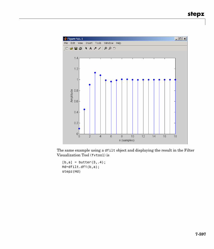
stepz
The same example using a dfilt object and displaying the result in the Filter Visualization Tool (fvtool) is
[b,a] = butter(3,.4);Hd=dfilt.df1(b,a);stepz(Hd)
7-597
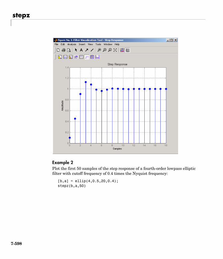
stepz
Example 2Plot the first 50 samples of the step response of a fourth-order lowpass elliptic filter with cutoff frequency of 0.4 times the Nyquist frequency:
[b,a] = ellip(4,0.5,20,0.4);stepz(b,a,50)
7-598
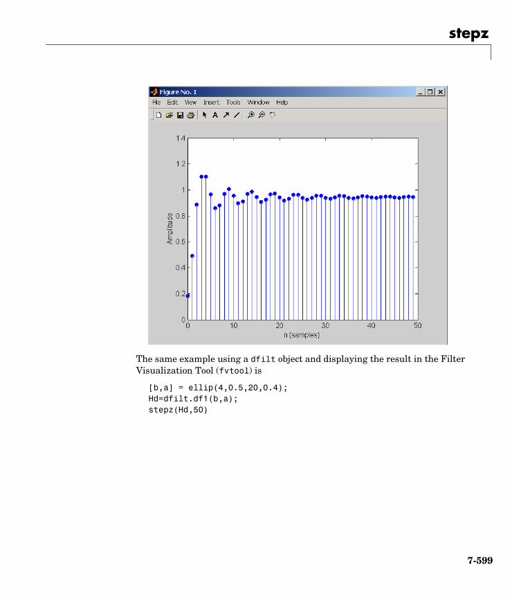
stepz
The same example using a dfilt object and displaying the result in the Filter Visualization Tool (fvtool) is
[b,a] = ellip(4,0.5,20,0.4);Hd=dfilt.df1(b,a);stepz(Hd,50)
7-599
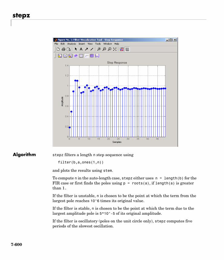
stepz
Algorithm stepz filters a length n step sequence using
filter(b,a,ones(1,n))
and plots the results using stem.
To compute n in the auto-length case, stepz either uses n = length(b) for the FIR case or first finds the poles using p = roots(a), if length(a) is greater than 1.
If the filter is unstable, n is chosen to be the point at which the term from the largest pole reaches 10^6 times its original value.
If the filter is stable, n is chosen to be the point at which the term due to the largest amplitude pole is 5*10^-5 of its original amplitude.
If the filter is oscillatory (poles on the unit circle only), stepz computes five periods of the slowest oscillation.
7-600

stepz
If the filter has both oscillatory and damped terms, n is chosen to equal five periods of the slowest oscillation or the point at which the term due to the largest (nonunity) amplitude pole is 5*10^-5 of its original amplitude, whichever is greater.
stepz also allows for delays in the numerator polynomial. The number of delays is incorporated into the computation for the number of samples.
See Also freqz, grpdelay, impz, phasez, zplane
7-601
stmcb
7stmcbPurpose Compute a linear model using Steiglitz-McBride iteration
Syntax [b,a] = stmcb(h,nb,na)[b,a] = stmcb(y,x,nb,na)[b,a] = stmcb(h,nb,na,niter)[b,a] = stmcb(y,x,nb,na,niter)[b,a] = stmcb(h,nb,na,niter,ai)[b,a] = stmcb(y,x,nb,na,niter,ai)
Description Steiglitz-McBride iteration is an algorithm for finding an IIR filter with a prescribed time domain impulse response. It has applications in both filter design and system identification (parametric modeling).
[b,a] = stmcb(h,nb,na) finds the coefficients b and a of the system b(z)/a(z) with approximate impulse response h, exactly nb zeros, and exactly na poles.
[b,a] = stmcb(y,x,nb,na) finds the system coefficients b and a of the system that, given x as input, has y as output. x and y must be the same length.
[b,a] = stmcb(h,nb,na,niter) and
[b,a] = stmcb(y,x,nb,na,niter) use niter iterations. The default for niter is 5.
[b,a] = stmcb(h,nb,na,niter,ai) and
[b,a] = stmcb(y,x,nb,na,niter,ai) use the vector ai as the initial estimate of the denominator coefficients. If ai is not specified, stmcb uses the output argument from [b,ai] = prony(h,0,na) as the vector ai.
stmcb returns the IIR filter coefficients in length nb+1 and na+1 row vectors b and a. The filter coefficients are ordered in descending powers of z.
Examples Approximate the impulse response of a Butterworth filter with a system of lower order:
[b,a] = butter(6,0.2);
H z( )B z( )A z( )----------- b 1( ) b 2( )z 1– b nb 1+( )z nb–+ + +
a 1( ) a 2( )z 1– a na 1+( )z na–+ + +--------------------------------------------------------------------------------------------= =
7-602
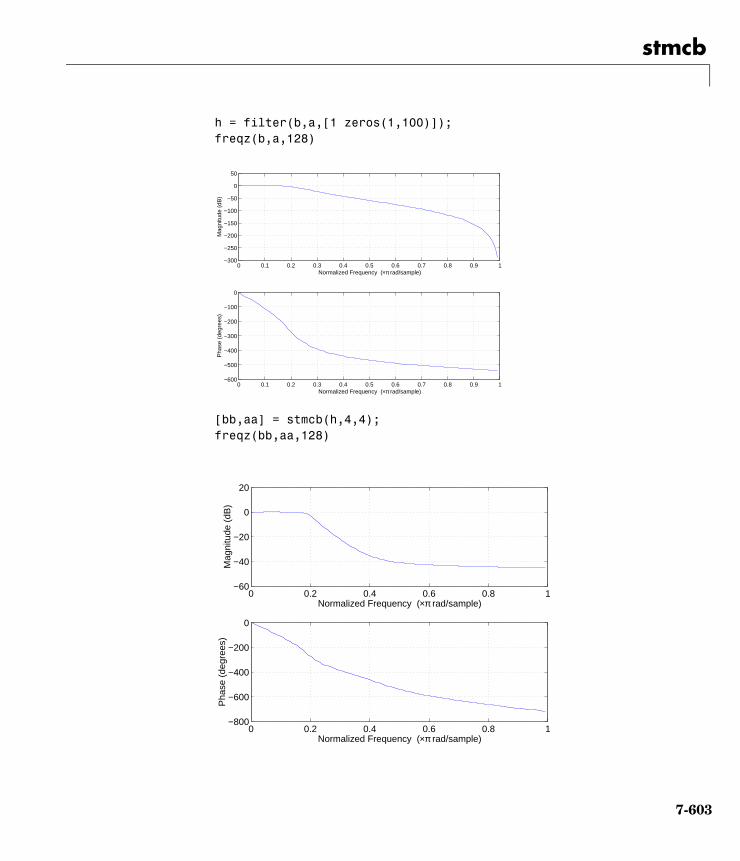
stmcb
h = filter(b,a,[1 zeros(1,100)]);freqz(b,a,128)
[bb,aa] = stmcb(h,4,4);freqz(bb,aa,128)
0 0.1 0.2 0.3 0.4 0.5 0.6 0.7 0.8 0.9 1−600
−500
−400
−300
−200
−100
0
Normalized Frequency (×π rad/sample)
Pha
se (
degr
ees)
0 0.1 0.2 0.3 0.4 0.5 0.6 0.7 0.8 0.9 1−300
−250
−200
−150
−100
−50
0
50
Normalized Frequency (×π rad/sample)
Mag
nitu
de (
dB)
0 0.2 0.4 0.6 0.8 1−800
−600
−400
−200
0
Normalized Frequency (×π rad/sample)
Pha
se (
degr
ees)
0 0.2 0.4 0.6 0.8 1−60
−40
−20
0
20
Normalized Frequency (×π rad/sample)
Mag
nitu
de (
dB)
7-603
stmcb
Algorithm stmcb attempts to minimize the squared error between the impulse response h of b(z)/a(z) and the input signal x.
stmcb iterates using two steps:
1 It prefilters h and x using 1/a(z).
2 It solves a system of linear equations for b and a using \.
stmcb repeats this process niter times. No checking is done to see if the b and a coefficients have converged in fewer than niter iterations.
Diagnostics If x and y have different lengths, stmcb produces this error message,
Input signal X and output signal Y must have the same length.
See Also levinson, lpc, aryule, prony
References [1] Steiglitz, K., and L.E. McBride, “A Technique for the Identification of Linear Systems,” IEEE Trans. Automatic Control, Vol. AC-10 (1965), pp. 461-464.
[2] Ljung, L., System Identification: Theory for the User, Prentice-Hall, Englewood Cliffs, NJ, 1987, p. 297.
mina b,
x i( ) h i( )– 2
i 0=
∞
∑
7-604
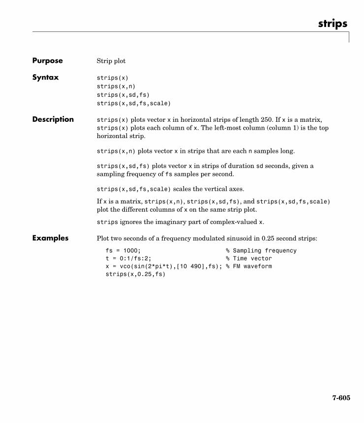
strips
7stripsPurpose Strip plot
Syntax strips(x)strips(x,n)strips(x,sd,fs)strips(x,sd,fs,scale)
Description strips(x) plots vector x in horizontal strips of length 250. If x is a matrix, strips(x) plots each column of x. The left-most column (column 1) is the top horizontal strip.
strips(x,n) plots vector x in strips that are each n samples long.
strips(x,sd,fs) plots vector x in strips of duration sd seconds, given a sampling frequency of fs samples per second.
strips(x,sd,fs,scale) scales the vertical axes.
If x is a matrix, strips(x,n), strips(x,sd,fs), and strips(x,sd,fs,scale) plot the different columns of x on the same strip plot.
strips ignores the imaginary part of complex-valued x.
Examples Plot two seconds of a frequency modulated sinusoid in 0.25 second strips:
fs = 1000; % Sampling frequencyt = 0:1/fs:2; % Time vectorx = vco(sin(2*pi*t),[10 490],fs); % FM waveformstrips(x,0.25,fs)
7-605
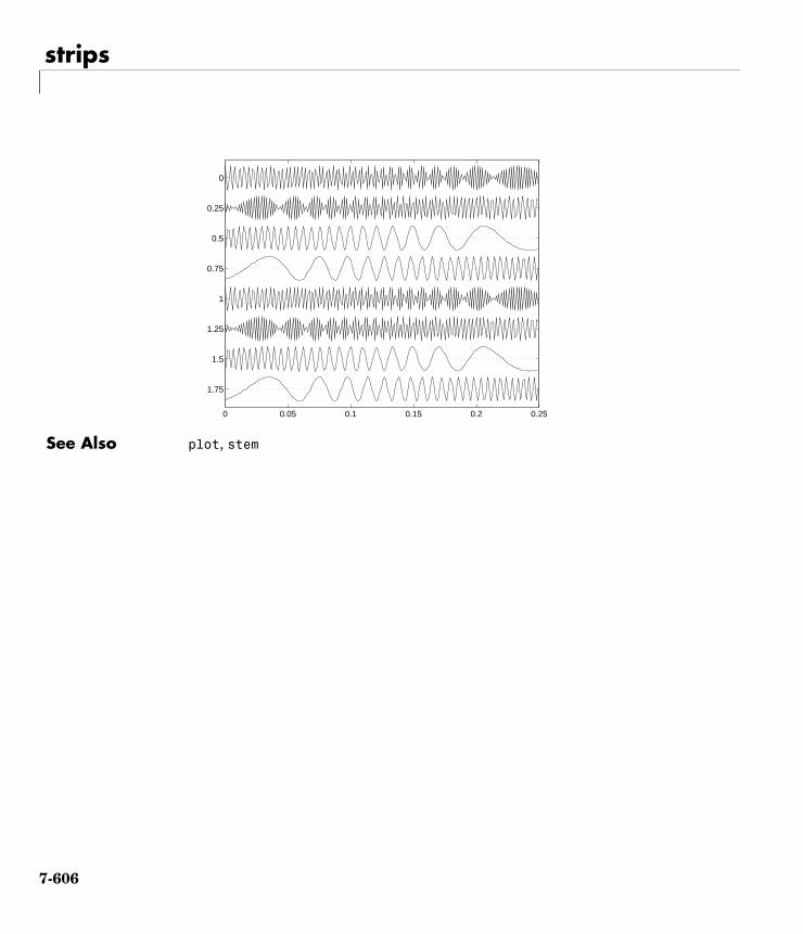
strips
See Also plot, stem
0 0.05 0.1 0.15 0.2 0.25
1.75
1.5
1.25
1
0.75
0.5
0.25
0
7-606
tf2latc
7tf2latcPurpose Convert transfer function filter parameters to lattice filter form
Syntax [k,v] = tf2latc(b,a)k = tf2latc(1,a)[k,v] = tf2latc(1,a)k = tf2latc(b)k = tf2latc(b,'phase')
Description [k,v] = tf2latc(b,a) finds the lattice parameters k and the ladder parameters v for an IIR (ARMA) lattice-ladder filter, normalized by a(1). Note that an error is generated if one or more of the lattice parameters are exactly equal to 1.
k = tf2latc(1,a) finds the lattice parameters k for an IIR all-pole (AR) lattice filter.
[k,v] = tf2latc(1,a) returns the scalar ladder coefficient at the correct position in vector v. All other elements of v are zero.
k = tf2latc(b) finds the lattice parameters k for an FIR (MA) lattice filter, normalized by b(1).
k = tf2latc(b,'phase') specifies the type of FIR (MA) lattice filter, where 'phase' is
• 'max', for a maximum phase filter.
• 'min', for a minimum phase filter.
See Also latc2tf, latcfilt, tf2sos, tf2ss, tf2zp, tf2zpk
7-607
tf2sos
7tf2sosPurpose Convert digital filter transfer function data to second-order sections form
Syntax [sos,g] = tf2sos(b,a)[sos,g] = tf2sos(b,a,'order')[sos,g] = tf2sos(b,a,'order','scale')sos = tf2sos(...)
Description tf2sos converts a transfer function representation of a given digital filter to an equivalent second-order section representation.
[sos,g] = tf2sos(b,a) finds a matrix sos in second-order section form with gain g that is equivalent to the digital filter represented by transfer function coefficient vectors a and b.
sos is an L-by-6 matrix
whose rows contain the numerator and denominator coefficients bik and aik of the second-order sections of H(z).
[sos,g] = tf2sos(b,a,'order') specifies the order of the rows in sos, where 'order' is
• 'down', to order the sections so the first row of sos contains the poles closest to the unit circle
H z( )B z( )A z( )-----------
b1 b2z 1– bn 1+ z n–+ + +
a1 a2z 1– am 1+ z m–+ + +------------------------------------------------------------------------= =
sos
b01 b11 b21 1 a11 a21
b02 b12 b22 1 a12 a22
b0L b1L b2L 1 a1L a2L
=
H z( ) g Hk z( )
k 1=
L
∏ gb0k b1kz 1– b2kz 2–+ +
1 a1kz 1– a2kz 2–+ +----------------------------------------------------------
k 1=
L
∏= =
7-608
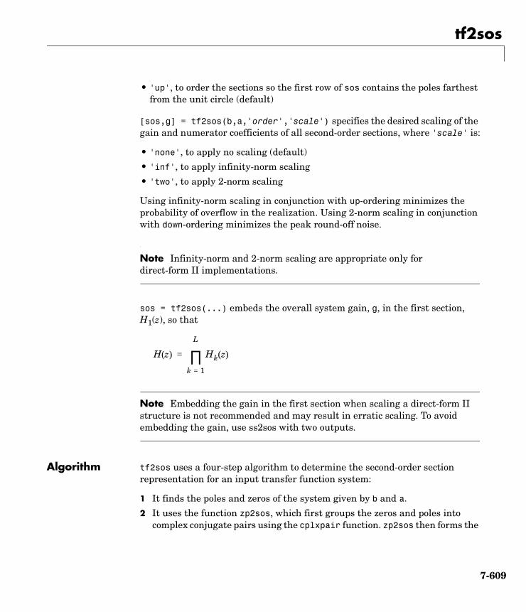
tf2sos
• 'up', to order the sections so the first row of sos contains the poles farthest from the unit circle (default)
[sos,g] = tf2sos(b,a,'order','scale') specifies the desired scaling of the gain and numerator coefficients of all second-order sections, where 'scale' is:
• 'none', to apply no scaling (default)
• 'inf', to apply infinity-norm scaling
• 'two', to apply 2-norm scaling
Using infinity-norm scaling in conjunction with up-ordering minimizes the probability of overflow in the realization. Using 2-norm scaling in conjunction with down-ordering minimizes the peak round-off noise.
Note Infinity-norm and 2-norm scaling are appropriate only for direct-form II implementations.
sos = tf2sos(...) embeds the overall system gain, g, in the first section, H1(z), so that
Note Embedding the gain in the first section when scaling a direct-form II structure is not recommended and may result in erratic scaling. To avoid embedding the gain, use ss2sos with two outputs.
Algorithm tf2sos uses a four-step algorithm to determine the second-order section representation for an input transfer function system:
1 It finds the poles and zeros of the system given by b and a.
2 It uses the function zp2sos, which first groups the zeros and poles into complex conjugate pairs using the cplxpair function. zp2sos then forms the
H z( ) Hk z( )
k 1=
L
∏=
7-609
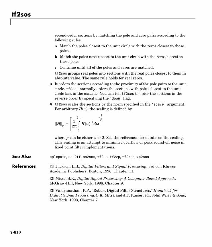
tf2sos
second-order sections by matching the pole and zero pairs according to the following rules:
a Match the poles closest to the unit circle with the zeros closest to those poles.
b Match the poles next closest to the unit circle with the zeros closest to those poles.
c Continue until all of the poles and zeros are matched.
tf2sos groups real poles into sections with the real poles closest to them in absolute value. The same rule holds for real zeros.
3 It orders the sections according to the proximity of the pole pairs to the unit circle. tf2sos normally orders the sections with poles closest to the unit circle last in the cascade. You can tell tf2sos to order the sections in the reverse order by specifying the 'down' flag.
4 tf2sos scales the sections by the norm specified in the 'scale' argument. For arbitrary H(ω), the scaling is defined by
where p can be either ∞ or 2. See the references for details on the scaling. This scaling is an attempt to minimize overflow or peak round-off noise in fixed point filter implementations.
See Also cplxpair, sos2tf, ss2sos, tf2ss, tf2zp, tf2zpk, zp2sos
References [1] Jackson, L.B., Digital Filters and Signal Processing, 3rd ed., Kluwer Academic Publishers, Boston, 1996, Chapter 11.
[2] Mitra, S.K., Digital Signal Processing: A Computer-Based Approach, McGraw-Hill, New York, 1998, Chapter 9.
[3] Vaidyanathan, P.P., “Robust Digital Filter Structures,” Handbook for Digital Signal Processing, S.K. Mitra and J.F. Kaiser, ed., John Wiley & Sons, New York, 1993, Chapter 7.
H p1
2π------ H ω( ) p ωd
0
2π
∫
1p---
=
7-610
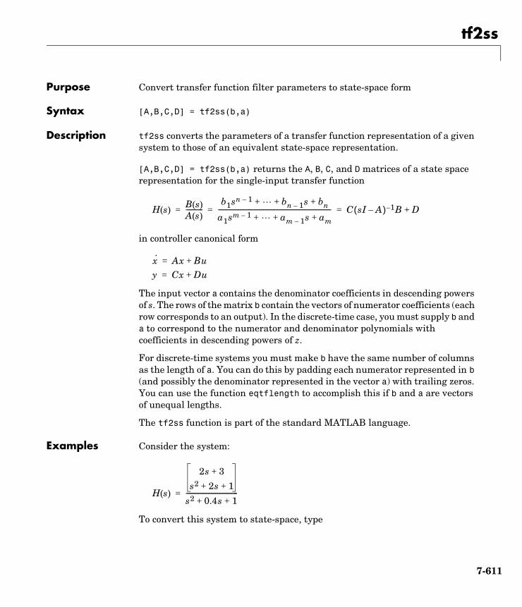
tf2ss
7tf2ssPurpose Convert transfer function filter parameters to state-space form
Syntax [A,B,C,D] = tf2ss(b,a)
Description tf2ss converts the parameters of a transfer function representation of a given system to those of an equivalent state-space representation.
[A,B,C,D] = tf2ss(b,a) returns the A, B, C, and D matrices of a state space representation for the single-input transfer function
in controller canonical form
The input vector a contains the denominator coefficients in descending powers of s. The rows of the matrix b contain the vectors of numerator coefficients (each row corresponds to an output). In the discrete-time case, you must supply b and a to correspond to the numerator and denominator polynomials with coefficients in descending powers of z.
For discrete-time systems you must make b have the same number of columns as the length of a. You can do this by padding each numerator represented in b (and possibly the denominator represented in the vector a) with trailing zeros. You can use the function eqtflength to accomplish this if b and a are vectors of unequal lengths.
The tf2ss function is part of the standard MATLAB language.
Examples Consider the system:
To convert this system to state-space, type
H s( )B s( )A s( )-----------
b1sn 1– bn 1– s bn+ + +
a1sm 1– am 1– s am+ + +------------------------------------------------------------------------ C sI A–( ) 1– B D+= = =
x· Ax Bu+=
y Cx Du+=
H s( )
2s 3+
s2 2s 1+ +
s2 0.4s 1+ +---------------------------------=
7-611
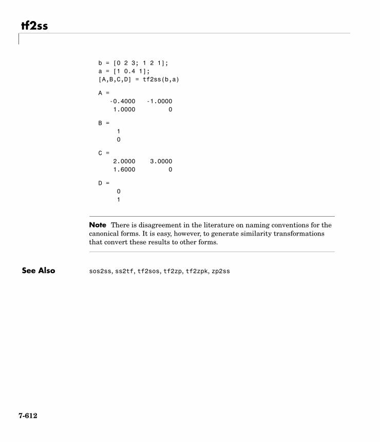
tf2ss
b = [0 2 3; 1 2 1];a = [1 0.4 1];[A,B,C,D] = tf2ss(b,a)
A = -0.4000 -1.0000 1.0000 0
B = 1 0
C = 2.0000 3.0000 1.6000 0
D = 0 1
Note There is disagreement in the literature on naming conventions for the canonical forms. It is easy, however, to generate similarity transformations that convert these results to other forms.
See Also sos2ss, ss2tf, tf2sos, tf2zp, tf2zpk, zp2ss
7-612
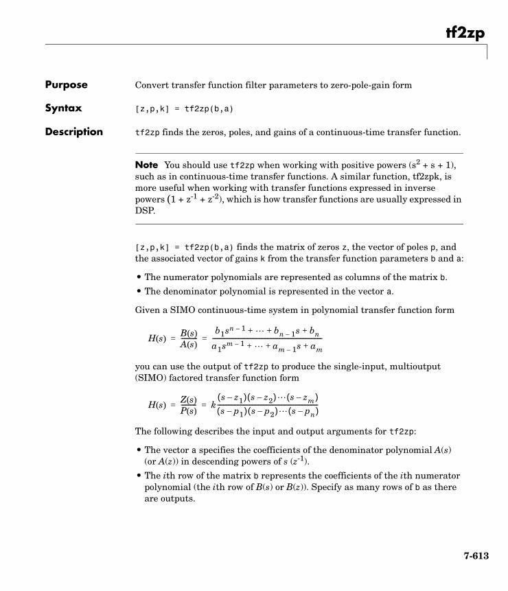
tf2zp
7tf2zpPurpose Convert transfer function filter parameters to zero-pole-gain form
Syntax [z,p,k] = tf2zp(b,a)
Description tf2zp finds the zeros, poles, and gains of a continuous-time transfer function.
Note You should use tf2zp when working with positive powers (s2 + s + 1), such as in continuous-time transfer functions. A similar function, tf2zpk, is more useful when working with transfer functions expressed in inverse powers (1 + z-1 + z-2), which is how transfer functions are usually expressed in DSP.
[z,p,k] = tf2zp(b,a) finds the matrix of zeros z, the vector of poles p, and the associated vector of gains k from the transfer function parameters b and a:
• The numerator polynomials are represented as columns of the matrix b.
• The denominator polynomial is represented in the vector a.
Given a SIMO continuous-time system in polynomial transfer function form
you can use the output of tf2zp to produce the single-input, multioutput (SIMO) factored transfer function form
The following describes the input and output arguments for tf2zp:
• The vector a specifies the coefficients of the denominator polynomial A(s) (or A(z)) in descending powers of s (z-1).
• The ith row of the matrix b represents the coefficients of the ith numerator polynomial (the ith row of B(s) or B(z)). Specify as many rows of b as there are outputs.
H s( )B s( )A s( )-----------
b1sn 1– bn 1– s bn+ + +
a1sm 1– am 1– s am+ + +------------------------------------------------------------------------= =
H s( )Z s( )P s( )---------- k
s z1–( ) s z2–( ) s zm–( )s p1–( ) s p2–( ) s pn–( )
------------------------------------------------------------------= =
7-613
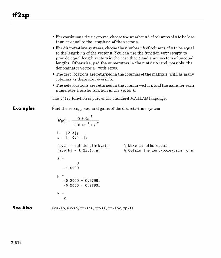
tf2zp
• For continuous-time systems, choose the number nb of columns of b to be less than or equal to the length na of the vector a.
• For discrete-time systems, choose the number nb of columns of b to be equal to the length na of the vector a. You can use the function eqtflength to provide equal length vectors in the case that b and a are vectors of unequal lengths. Otherwise, pad the numerators in the matrix b (and, possibly, the denominator vector a) with zeros.
• The zero locations are returned in the columns of the matrix z, with as many columns as there are rows in b.
• The pole locations are returned in the column vector p and the gains for each numerator transfer function in the vector k.
The tf2zp function is part of the standard MATLAB language.
Examples Find the zeros, poles, and gains of the discrete-time system:
b = [2 3];a = [1 0.4 1];
[b,a] = eqtflength(b,a); % Make lengths equal.[z,p,k] = tf2zp(b,a) % Obtain the zero-pole-gain form.
z = 0 -1.5000
p = -0.2000 + 0.9798i -0.2000 - 0.9798i
k = 2
See Also sos2zp, ss2zp, tf2sos, tf2ss, tf2zpk, zp2tf
H z( )2 3z 1–
+
1 0.4z 1– z 2–+ +
-----------------------------------------=
7-614
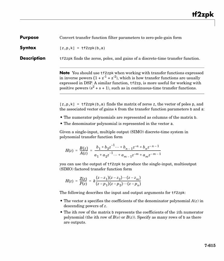
tf2zpk
7tf2zpkPurpose Convert transfer function filter parameters to zero-pole-gain form
Syntax [z,p,k] = tf2zpk(b,a)
Description tf2zpk finds the zeros, poles, and gains of a discrete-time transfer function.
Note You should use tf2zpk when working with transfer functions expressed in inverse powers (1 + z-1 + z-2), which is how transfer functions are usually expressed in DSP. A similar function, tf2zp, is more useful for working with positive powers (s2 + s + 1), such as in continuous-time transfer functions.
[z,p,k] = tf2zpk(b,a) finds the matrix of zeros z, the vector of poles p, and the associated vector of gains k from the transfer function parameters b and a:
• The numerator polynomials are represented as columns of the matrix b.
• The denominator polynomial is represented in the vector a.
Given a single-input, multiple output (SIMO) discrete-time system in polynomial transfer function form
you can use the output of tf2zpk to produce the single-input, multioutput (SIMO) factored transfer function form
The following describes the input and output arguments for tf2zpk:
• The vector a specifies the coefficients of the denominator polynomial A(z) in descending powers of z.
• The ith row of the matrix b represents the coefficients of the ith numerator polynomial (the ith row of B(s) or B(z)). Specify as many rows of b as there are outputs.
H z( )B z( )A z( )------------
b1 b2z 1– bn 1– z n– bnz n– 1–+ + +
a1 a2z 1– am 1– z m– amz m– 1–+ + +---------------------------------------------------------------------------------------------------= =
H z( )Z z( )P z( )---------- k
z z1–( ) z z2–( ) z zm–( )z p1–( ) z p2–( ) z pn–( )
-------------------------------------------------------------------= =
7-615

tf2zpk
• The zero locations are returned in the columns of the matrix z, with as many columns as there are rows in b.
• The pole locations are returned in the column vector p and the gains for each numerator transfer function in the vector k.
Examples Find the poles, zeros, and gain of a Butterworth filter:
[b,a] = butter(3,.4);[z,p,k] = tf2zpk(b,a)
z = -1.0000 -1.0000 + 0.0000i -1.0000 - 0.0000i
p = 0.2094 + 0.5582i 0.2094 - 0.5582i 0.1584
k = 0.0985
See Also sos2zp, ss2zp, tf2sos, tf2ss, tf2zp, zp2tf
7-616
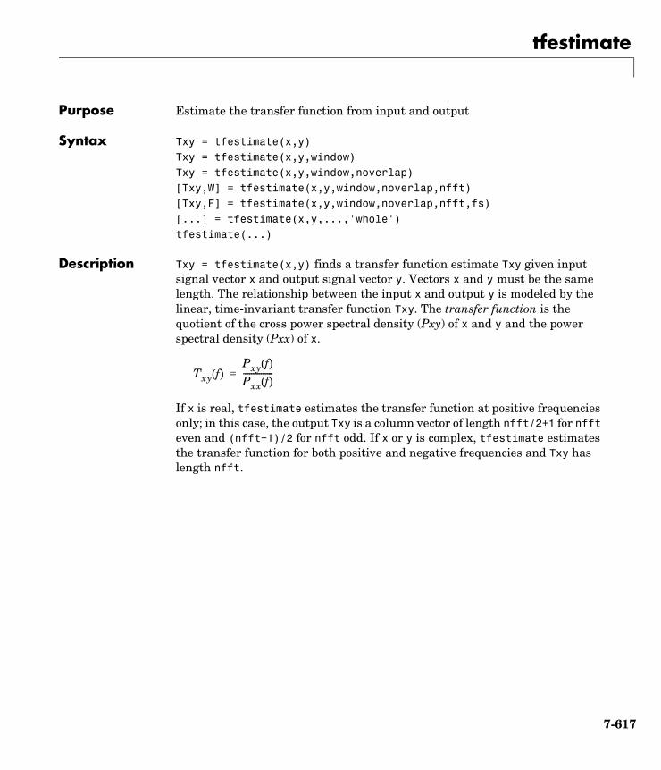
tfestimate
7tfestimatePurpose Estimate the transfer function from input and output
Syntax Txy = tfestimate(x,y)Txy = tfestimate(x,y,window)Txy = tfestimate(x,y,window,noverlap)[Txy,W] = tfestimate(x,y,window,noverlap,nfft)[Txy,F] = tfestimate(x,y,window,noverlap,nfft,fs)[...] = tfestimate(x,y,...,'whole')tfestimate(...)
Description Txy = tfestimate(x,y) finds a transfer function estimate Txy given input signal vector x and output signal vector y. Vectors x and y must be the same length. The relationship between the input x and output y is modeled by the linear, time-invariant transfer function Txy. The transfer function is the quotient of the cross power spectral density (Pxy) of x and y and the power spectral density (Pxx) of x.
If x is real, tfestimate estimates the transfer function at positive frequencies only; in this case, the output Txy is a column vector of length nfft/2+1 for nfft even and (nfft+1)/2 for nfft odd. If x or y is complex, tfestimate estimates the transfer function for both positive and negative frequencies and Txy has length nfft.
Txy f( )Pxy f( )
Pxx f( )---------------=
7-617
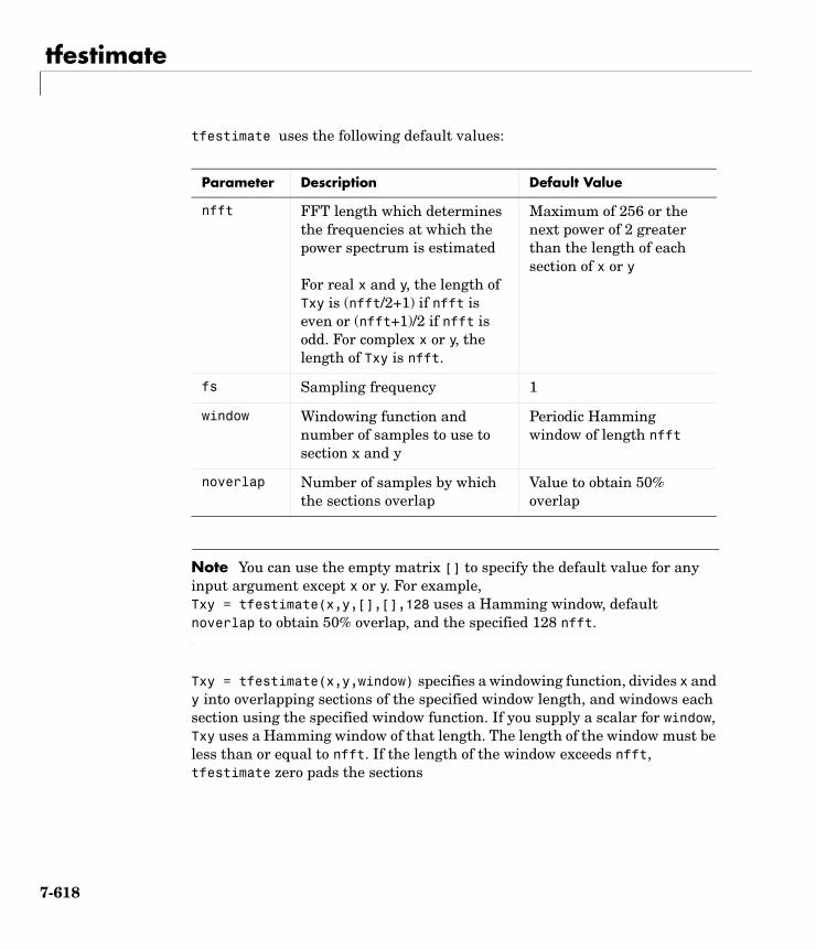
tfestimate
tfestimate uses the following default values:
Note You can use the empty matrix [] to specify the default value for any input argument except x or y. For example, Txy = tfestimate(x,y,[],[],128 uses a Hamming window, default noverlap to obtain 50% overlap, and the specified 128 nfft.
Txy = tfestimate(x,y,window) specifies a windowing function, divides x and y into overlapping sections of the specified window length, and windows each section using the specified window function. If you supply a scalar for window, Txy uses a Hamming window of that length. The length of the window must be less than or equal to nfft. If the length of the window exceeds nfft, tfestimate zero pads the sections
Parameter Description Default Value
nfft FFT length which determines the frequencies at which the power spectrum is estimated
For real x and y, the length of Txy is (nfft/2+1) if nfft is even or (nfft+1)/2 if nfft is odd. For complex x or y, the length of Txy is nfft.
Maximum of 256 or the next power of 2 greater than the length of each section of x or y
fs Sampling frequency 1
window Windowing function and number of samples to use to section x and y
Periodic Hamming window of length nfft
noverlap Number of samples by which the sections overlap
Value to obtain 50% overlap
7-618
tfestimate
Txy = tfestimate(x,y,window,noverlap) overlaps the sections of x by noverlap samples. noverlap must be an integer smaller than the length of window.
[Txy,W] = tfestimate(x,y,window,noverlap,nfft) uses the specified FFT length nfft in estimating the PSD and CPSD estimates for the transfer function. It also returns W, which is the vector of normalized frequencies (inrad/sample) at which the tfestimate is estimated. For real signals, the range of W is [0, pi] when nfft is even and [0, pi) when nfft is odd. For complex signals, the range of W is [0, 2pi).
[Txy,F] = tfestimate(x,y,window,noverlap,nfft,fs) returns Txy as a function of frequency and a vector F of frequencies at which tfestimate estimates the transfer function. fs is the sampling frequency in Hz. F is the same size as Txy, so plot(f,Txy) plots the transfer function estimate versus properly scaled frequency. For real signals, the range of F is [0, fs/2] when nfft is even and [0, fs/2) when nfft is odd. For complex signals, the range of F is [0, fs).
[...] = tfestimate(x,y,...,'whole') returns a transfer function estimate with frequencies that range over the whole Nyquist interval. Specifying 'half' uses half the Nyquist interval.
tfestimate(...) with no output arguments plots the transfer function estimate in the current figure window.
Examples Compute and plot the transfer function estimate between two colored noise sequences x and y:
h = fir1(30,0.2,rectwin(31));x = randn(16384,1);y = filter(h,1,x);tfestimate(x,y,1024,[],[],512)
7-619
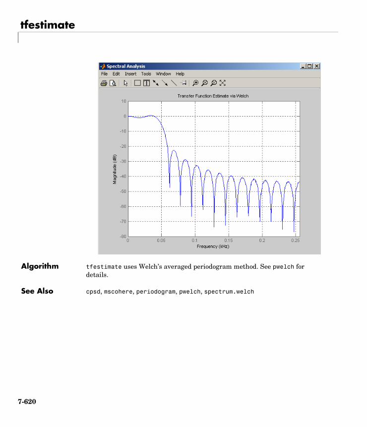
tfestimate
Algorithm tfestimate uses Welch’s averaged periodogram method. See pwelch for details.
See Also cpsd, mscohere, periodogram, pwelch, spectrum.welch
7-620
triang
7triangPurpose Compute a triangular window
Syntax w = triang(n)
Description triang(n) returns an n-point triangular window in the column vector w. The coefficients of a triangular window are:
For n odd:
For n even:
The triangular window is very similar to a Bartlett window. The Bartlett window always ends with zeros at samples 1 and n, while the triangular window is nonzero at those points. For n odd, the center n-2 points of triang(n-2) are equivalent to bartlett(n).
Examples Create a 200-point triangular window and plot the result using WVTool.
N=200;wvtool(triang(N))
w k[ ]
2kn 1+------------- 1 k n 1+
2-------------≤ ≤,
2 n k 1+–( )n 1+
------------------------------- n 1+2
------------- k< n≤,
=
w k[ ]
2k 1–n
---------------- 1 k n2---≤ ≤,
2 n k–( ) 1+n
------------------------------- n2--- 1+ k n≤ ≤,
=
7-621
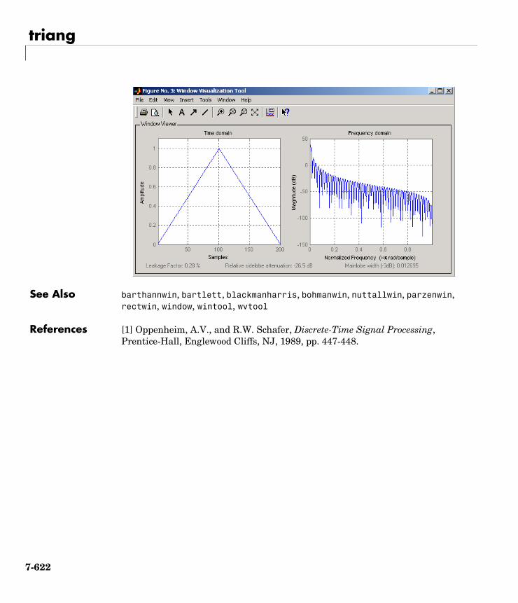
triang
See Also barthannwin, bartlett, blackmanharris, bohmanwin, nuttallwin, parzenwin, rectwin, window, wintool, wvtool
References [1] Oppenheim, A.V., and R.W. Schafer, Discrete-Time Signal Processing, Prentice-Hall, Englewood Cliffs, NJ, 1989, pp. 447-448.
7-622
tripuls
7tripulsPurpose Generate a sampled aperiodic triangle
Syntax y = tripuls(T)y = tripuls(T,w)y = tripuls(T,w,s)
Description y = tripuls(T) returns a continuous, aperiodic, symmetric, unity-height triangular pulse at the times indicated in array T, centered about T=0 and with a default width of 1.
y = tripuls(T,w) generates a triangular pulse of width w.
y = tripuls(T,w,s) generates a triangular pulse with skew s, where -1 < s < 1. When s is 0, a symmetric triangular pulse is generated.
See Also chirp, cos, diric, gauspuls, pulstran, rectpuls, sawtooth, sin, square, tripuls
7-623
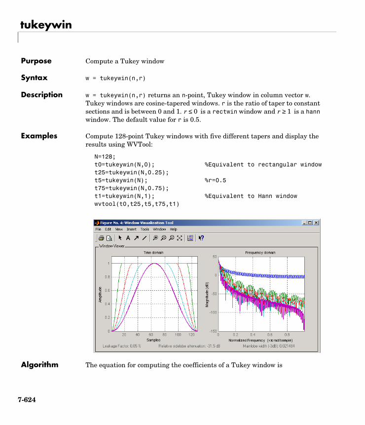
tukeywin
7tukeywinPurpose Compute a Tukey window
Syntax w = tukeywin(n,r)
Description w = tukeywin(n,r) returns an n-point, Tukey window in column vector w. Tukey windows are cosine-tapered windows. r is the ratio of taper to constant sections and is between 0 and 1. is a rectwin window and is a hann window. The default value for r is 0.5.
Examples Compute 128-point Tukey windows with five different tapers and display the results using WVTool:
N=128;t0=tukeywin(N,0); %Equivalent to rectangular windowt25=tukeywin(N,0.25);t5=tukeywin(N); %r=0.5t75=tukeywin(N,0.75);t1=tukeywin(N,1); %Equivalent to Hann windowwvtool(t0,t25,t5,t75,t1)
Algorithm The equation for computing the coefficients of a Tukey window is
r 0≤ r 1≥
7-624
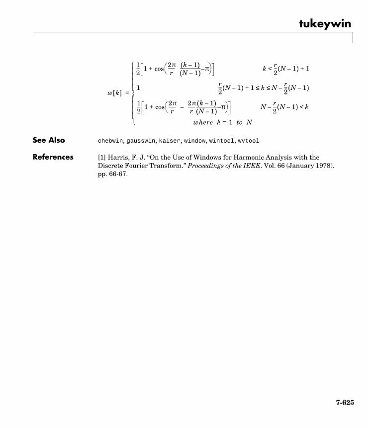
tukeywin
See Also chebwin, gausswin, kaiser, window, wintool, wvtool
References [1] Harris, F. J. “On the Use of Windows for Harmonic Analysis with the Discrete Fourier Transform.” Proceedings of the IEEE. Vol. 66 (January 1978). pp. 66-67.
w k[ ]
12--- 1 2π
r------ k 1–( )
N 1–( )------------------- π–
cos+ k r2--- N 1–( ) 1+<
1 r2--- N 1–( ) 1+ k N r
2--- N 1–( )–≤ ≤
12--- 1 2π
r------ 2π
r------–
k 1–( )N 1–( )
------------------- π– cos+ N r
2--- N 1–( )– k<
where k 1= to N
=
7-625
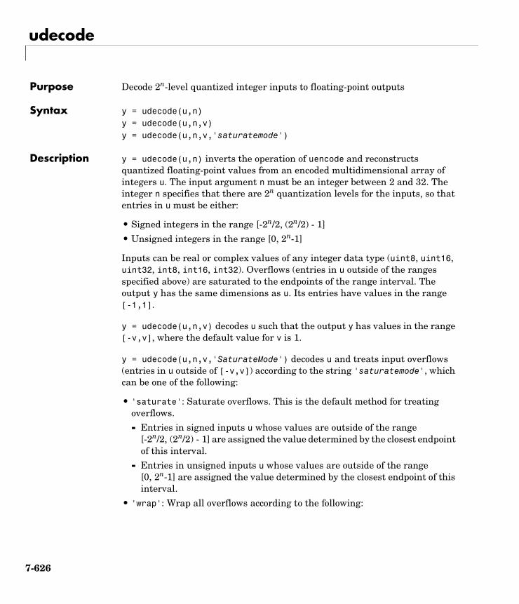
udecode
7udecodePurpose Decode 2n-level quantized integer inputs to floating-point outputs
Syntax y = udecode(u,n)y = udecode(u,n,v)y = udecode(u,n,v,'saturatemode')
Description y = udecode(u,n) inverts the operation of uencode and reconstructs quantized floating-point values from an encoded multidimensional array of integers u. The input argument n must be an integer between 2 and 32. The integer n specifies that there are 2n quantization levels for the inputs, so that entries in u must be either:
• Signed integers in the range [-2n/2, (2n/2) - 1]
• Unsigned integers in the range [0, 2n-1]
Inputs can be real or complex values of any integer data type (uint8, uint16, uint32, int8, int16, int32). Overflows (entries in u outside of the ranges specified above) are saturated to the endpoints of the range interval. The output y has the same dimensions as u. Its entries have values in the range [-1,1].
y = udecode(u,n,v) decodes u such that the output y has values in the range [-v,v], where the default value for v is 1.
y = udecode(u,n,v,'SaturateMode') decodes u and treats input overflows (entries in u outside of [-v,v]) according to the string 'saturatemode', which can be one of the following:
• 'saturate': Saturate overflows. This is the default method for treating overflows.
- Entries in signed inputs u whose values are outside of the range [-2n/2, (2n/2) - 1] are assigned the value determined by the closest endpoint of this interval.
- Entries in unsigned inputs u whose values are outside of the range [0, 2n-1] are assigned the value determined by the closest endpoint of this interval.
• 'wrap': Wrap all overflows according to the following:
7-626
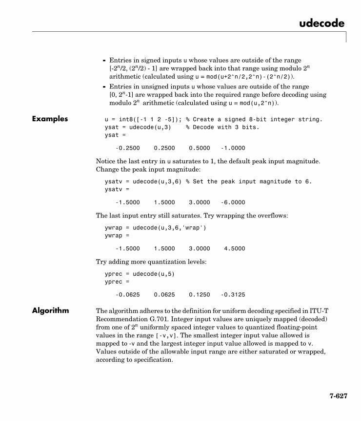
udecode
- Entries in signed inputs u whose values are outside of the range [-2n/2, (2n/2) - 1] are wrapped back into that range using modulo 2n
arithmetic (calculated using u = mod(u+2^n/2,2^n)-(2^n/2)).
- Entries in unsigned inputs u whose values are outside of the range [0, 2n-1] are wrapped back into the required range before decoding using modulo 2n arithmetic (calculated using u = mod(u,2^n)).
Examples u = int8([-1 1 2 -5]); % Create a signed 8-bit integer string.ysat = udecode(u,3) % Decode with 3 bits.ysat =
-0.2500 0.2500 0.5000 -1.0000
Notice the last entry in u saturates to 1, the default peak input magnitude. Change the peak input magnitude:
ysatv = udecode(u,3,6) % Set the peak input magnitude to 6.ysatv =
-1.5000 1.5000 3.0000 -6.0000
The last input entry still saturates. Try wrapping the overflows:
ywrap = udecode(u,3,6,'wrap')ywrap =
-1.5000 1.5000 3.0000 4.5000
Try adding more quantization levels:
yprec = udecode(u,5)yprec =
-0.0625 0.0625 0.1250 -0.3125
Algorithm The algorithm adheres to the definition for uniform decoding specified in ITU-T Recommendation G.701. Integer input values are uniquely mapped (decoded) from one of 2n uniformly spaced integer values to quantized floating-point values in the range [-v,v]. The smallest integer input value allowed is mapped to -v and the largest integer input value allowed is mapped to v. Values outside of the allowable input range are either saturated or wrapped, according to specification.
7-627
udecode
The real and imaginary components of complex inputs are decoded independently.
See Also uencode
References General Aspects of Digital Transmission Systems: Vocabulary of Digital Transmission and Multiplexing, and Pulse Code Modulation (PCM) Terms, International Telecommunication Union, ITU-T Recommendation G.701, March, 1993.
7-628
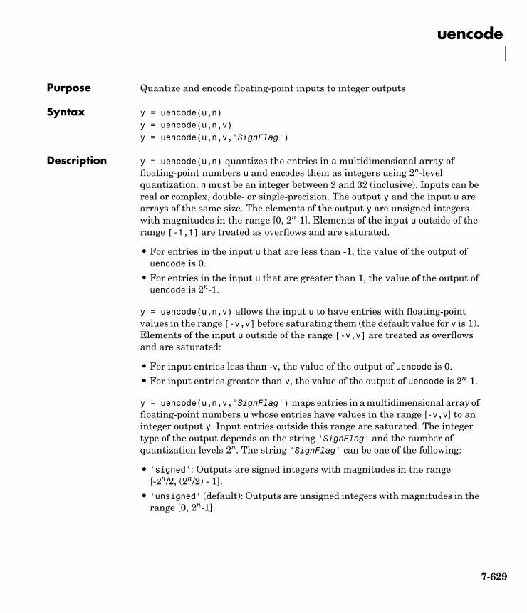
uencode
7uencodePurpose Quantize and encode floating-point inputs to integer outputs
Syntax y = uencode(u,n)y = uencode(u,n,v)y = uencode(u,n,v,'SignFlag')
Description y = uencode(u,n) quantizes the entries in a multidimensional array of floating-point numbers u and encodes them as integers using 2n-level quantization. n must be an integer between 2 and 32 (inclusive). Inputs can be real or complex, double- or single-precision. The output y and the input u are arrays of the same size. The elements of the output y are unsigned integers with magnitudes in the range [0, 2n-1]. Elements of the input u outside of the range [-1,1] are treated as overflows and are saturated.
• For entries in the input u that are less than -1, the value of the output of uencode is 0.
• For entries in the input u that are greater than 1, the value of the output of uencode is 2n-1.
y = uencode(u,n,v) allows the input u to have entries with floating-point values in the range [-v,v] before saturating them (the default value for v is 1). Elements of the input u outside of the range [-v,v] are treated as overflows and are saturated:
• For input entries less than -v, the value of the output of uencode is 0.
• For input entries greater than v, the value of the output of uencode is 2n-1.
y = uencode(u,n,v,'SignFlag') maps entries in a multidimensional array of floating-point numbers u whose entries have values in the range [-v,v] to an integer output y. Input entries outside this range are saturated. The integer type of the output depends on the string 'SignFlag' and the number of quantization levels 2n. The string 'SignFlag' can be one of the following:
• 'signed': Outputs are signed integers with magnitudes in the range [-2n/2, (2n/2) - 1].
• 'unsigned' (default): Outputs are unsigned integers with magnitudes in the range [0, 2n-1].
7-629
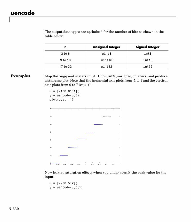
uencode
The output data types are optimized for the number of bits as shown in the table below.
Examples Map floating-point scalars in [-1, 1] to uint8 (unsigned) integers, and produce a staircase plot. Note that the horizontal axis plots from -1 to 1 and the vertical axis plots from 0 to 7 (2^3-1):
u = [-1:0.01:1];y = uencode(u,3);plot(u,y,'.')
Now look at saturation effects when you under specify the peak value for the input:
u = [-2:0.5:2];y = uencode(u,5,1)
n Unsigned Integer Signed Integer
2 to 8 uint8 int8
9 to 16 uint16 int16
17 to 32 uint32 int32
−1 −0.8 −0.6 −0.4 −0.2 0 0.2 0.4 0.6 0.8 10
1
2
3
4
5
6
7
7-630
uencode
y = 0 0 0 8 16 24 31 31 31
Now look at the output for
u = [-2:0.5:2];y = uencode(u,5,2,'signed')
y = -8 -4 0 4 8 12 16 20 23
Algorithm uencode maps the floating-point input value to an integer value determined by the requirement for 2n levels of quantization. This encoding adheres to the definition for uniform encoding specified in ITU-T Recommendation G.701. The input range [-v,v] is divided into 2n evenly spaced intervals. Input entries in the range [-v,v] are first quantized according to this subdivision of the input range, and then mapped to one of 2n integers. The range of the output depends on whether or not you specify that you want signed integers.
See Also udecode
References General Aspects of Digital Transmission Systems: Vocabulary of Digital Transmission and Multiplexing, and Pulse Code Modulation (PCM) Terms, International Telecommunication Union, ITU-T Recommendation G.701, March, 1993.
7-631

unwrap
7unwrapPurpose Unwrap phase angles
unwrap is a MATLAB function.
7-632
upfirdn
7upfirdnPurpose Upsample, apply an FIR filter, and downsample
Syntax yout = upfirdn(xin,h)yout = upfirdn(xin,h,p)yout = upfirdn(xin,h,p,q)
Description upfirdn performs a cascade of three operations:
1 Upsampling the input data in the matrix xin by a factor of the integer p (inserting zeros)
2 FIR filtering the upsampled signal data with the impulse response sequence given in the vector or matrix h
3 Downsampling the result by a factor of the integer q (throwing away samples)
upfirdn has been implemented as a MEX-file for maximum speed, so only the outputs actually needed are computed. The FIR filter is usually a lowpass filter, which you must design using another function such as firpm or fir1.
Note The function resample performs an FIR design using firls, followed by rate changing implemented with upfirdn.
yout = upfirdn(xin,h) filters the input signal xin with the FIR filter having impulse response h. If xin is a row or column vector, then it represents a single signal. If xin is a matrix, then each column is filtered independently. If h is a row or column vector, then it represents one FIR filter. If h is a matrix, then each column is a separate FIR impulse response sequence. If yout is a row or column vector, then it represents one signal. If yout is a matrix, then each column is a separate output. No upsampling or downsampling is implemented with this syntax.
yout = upfirdn(xin,h,p) specifies the integer upsampling factor p, where p has a default value of 1.
yout = upfirdn(xin,h,p,q) specifies the integer downsampling factor q, where q has a default value of 1.
7-633
upfirdn
Note Since upfirdn performs convolution and rate changing, the yout signals have a different length than xin. The number of rows of yout is approximately p/q times the number of rows of xin.
Remarks Usually the inputs xin and the filter h are vectors, in which case only one output signal is produced. However, when these arguments are arrays, each column is treated as a separate signal or filter. Valid combinations are:
1 xin is a vector and h is a vector.
There is one filter and one signal, so the function convolves xin with h. The output signal yout is a row vector if xin is a row; otherwise, yout is a column vector.
2 xin is a matrix and h is a vector.
There is one filter and many signals, so the function convolves h with each column of xin. The resulting yout will be an matrix with the same number of columns as xin.
3 xin is a vector and h is a matrix.
There are many filters and one signal, so the function convolves each column of h with xin. The resulting yout will be an matrix with the same number of columns as h.
4 xin is a matrix and h is a matrix, both with the same number of columns.
There are many filters and many signals, so the function convolves corresponding columns of xin and h. The resulting yout is an matrix with the same number of columns as xin and h.
Examples If both p and q are equal to 1 (that is, there is no rate changing), the result is ordinary convolution of two signals (equivalent to conv):
yy = upfirdn(xx,hh);
This example implements a seven-channel filter bank by convolving seven different filters with one input signal, then downsamples by five:
% Assume that hh is an L-by-7 array of filters.yy = upfirdn(xx,hh,1,5);
7-634
upfirdn
Implement a rate change from 44.1 kHz (CD sampling rate) to 48 kHz (DAT rate), a ratio of 160/147. This requires a lowpass filter with cutoff frequency at ωc = 2π/160:
% Design lowpass filter with cutoff at 1/160th of fs.
hh = fir1(300,1/160); % Need a very long lowpass filteryy = upfirdn(xx,hh,160,147);
In this example, the filter design and resampling are separate steps. Note that resample would do both steps as one.
Algorithm upfirdn uses a polyphase interpolation structure. The number of multiply-add operations in the polyphase structure is approximately (LhLx-pLx)/q where Lh and Lx are the lengths of h[n] and x[n], respectively.
A more accurate flops count is computed in the program, but the actual count is still approximate. For long signals x[n], the formula is often exact.
Diagnostics If p and q are large and do not have many common factors, you may see this message:
Filter length is too large - reduce problem complexity.
Instead, you should use an interpolation function, such as interp1, to perform the resampling and then filter the input.
See Also conv, decimate, downsample, filter, interp, intfilt, resample, upsample
References [1] Crochiere, R.E., and L.R. Rabiner, Multi-Rate Signal Processing, Prentice-Hall, Englewood Cliffs, NJ, 1983, pp. 88-91.
[2] Crochiere, R.E., “A General Program to Perform Sampling Rate Conversion of Data by Rational Ratios,” Programs for Digital Signal Processing, IEEE Press, New York, 1979, pp. 8.2-1 to 8.2-7.
7-635
upsample
7upsamplePurpose Increase the sampling rate of the input signal
Syntax y = upsample(x,n)y = upsample(x,n,phase)
Description y = upsample(x,n) increases the sampling rate of x by inserting n-1 zeros between samples. x can be a vector or a matrix. If x is a matrix, each column is considered a separate sequence. The upsampled y has x*n samples.
y = upsample(x,n,phase) specifies the number of samples by which to offset the upsampled sequence. phase must be an integer from 0 to n-1.
Examples Increase the sampling rate of a sequence by 3:
x = [1 2 3 4];y = upsample(x,3);x,y
x =1 2 3 4
y =1 0 0 2 0 0 3 0 0 4 0 0
Increase the sampling rate of the sequence by 3 and add a phase offset of 2:
x = [1 2 3 4];y = upsample(x,3,2);x,y
x =1 2 3 4
y =0 0 1 0 0 2 0 0 3 0 0 4
Increase the sampling rate of a matrix by 3:
x = [1 2; 3 4; 5 6;];y = upsample(x,3);x,y
x =
7-636

upsample
1 23 45 6
y = 1 20 00 03 40 00 05 60 00 0
See Also decimate, downsample, interp, interp1, resample, spline, upfirdn
7-637
vco
7vcoPurpose Voltage controlled oscillator
Syntax y = vco(x,fc,fs)y = vco(x,[Fmin Fmax],fs)
Description y = vco(x,fc,fs) creates a signal that oscillates at a frequency determined by the real input vector or array x with sampling frequency fs. fc is the carrier or reference frequency; when x is 0, y is an fc Hz cosine with amplitude 1 sampled at fs Hz. x ranges from -1 to 1, where x = -1 corresponds to 0 frequency output, x = 0 corresponds to fc, and x = 1 corresponds to 2*fc. Output y is the same size as x.
y = vco(x,[Fmin Fmax],fs) scales the frequency modulation range so that ±1 values of x yield oscillations of Fmin Hz and Fmax Hz respectively. For best results, Fmin and Fmax should be in the range 0 to fs/2.
By default, fs is 1 and fc is fs/4.
If x is a matrix, vco produces a matrix whose columns oscillate according to the columns of x.
Examples Generate two seconds of a signal sampled at 10,000 samples/second whose instantaneous frequency is a triangle function of time:
fs = 10000;t = 0:1/fs:2;x = vco(sawtooth(2*pi*t,0.75),[0.1 0.4]*fs,fs);
Plot the spectrogram of the generated signal:
specgram(x,512,fs,kaiser(256,5),220)
7-638
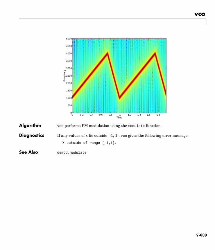
vco
Algorithm vco performs FM modulation using the modulate function.
Diagnostics If any values of x lie outside [-1, 1], vco gives the following error message.
X outside of range [-1,1].
See Also demod, modulate
Time
Fre
quen
cy
0 0.2 0.4 0.6 0.8 1 1.2 1.4 1.6 1.80
500
1000
1500
2000
2500
3000
3500
4000
4500
5000
7-639
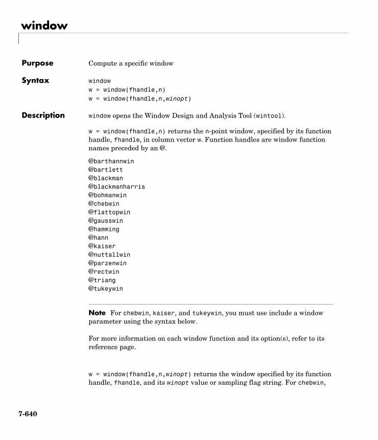
window
7windowPurpose Compute a specific window
Syntax windoww = window(fhandle,n)w = window(fhandle,n,winopt)
Description window opens the Window Design and Analysis Tool (wintool).
w = window(fhandle,n) returns the n-point window, specified by its function handle, fhandle, in column vector w. Function handles are window function names preceded by an @.
@barthannwin @bartlett @blackman @blackmanharris @bohmanwin @chebwin @flattopwin @gausswin @hamming @hann @kaiser @nuttallwin @parzenwin @rectwin @triang @tukeywin
Note For chebwin, kaiser, and tukeywin, you must use include a window parameter using the syntax below.
For more information on each window function and its option(s), refer to its reference page.
w = window(fhandle,n,winopt) returns the window specified by its function handle, fhandle, and its winopt value or sampling flag string. For chebwin,
7-640
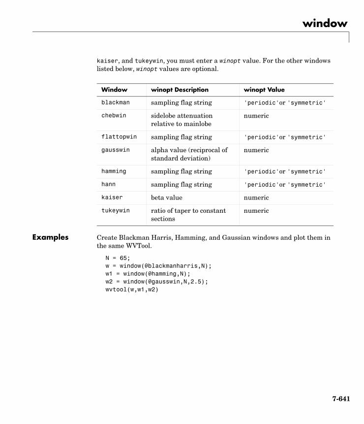
window
kaiser, and tukeywin, you must enter a winopt value. For the other windows listed below, winopt values are optional.
Examples Create Blackman Harris, Hamming, and Gaussian windows and plot them in the same WVTool.
N = 65;w = window(@blackmanharris,N);w1 = window(@hamming,N); w2 = window(@gausswin,N,2.5); wvtool(w,w1,w2)
Window winopt Description winopt Value
blackman sampling flag string 'periodic'or 'symmetric'
chebwin sidelobe attenuation relative to mainlobe
numeric
flattopwin sampling flag string 'periodic'or 'symmetric'
gausswin alpha value (reciprocal of standard deviation)
numeric
hamming sampling flag string 'periodic'or 'symmetric'
hann sampling flag string 'periodic'or 'symmetric'
kaiser beta value numeric
tukeywin ratio of taper to constant sections
numeric
7-641
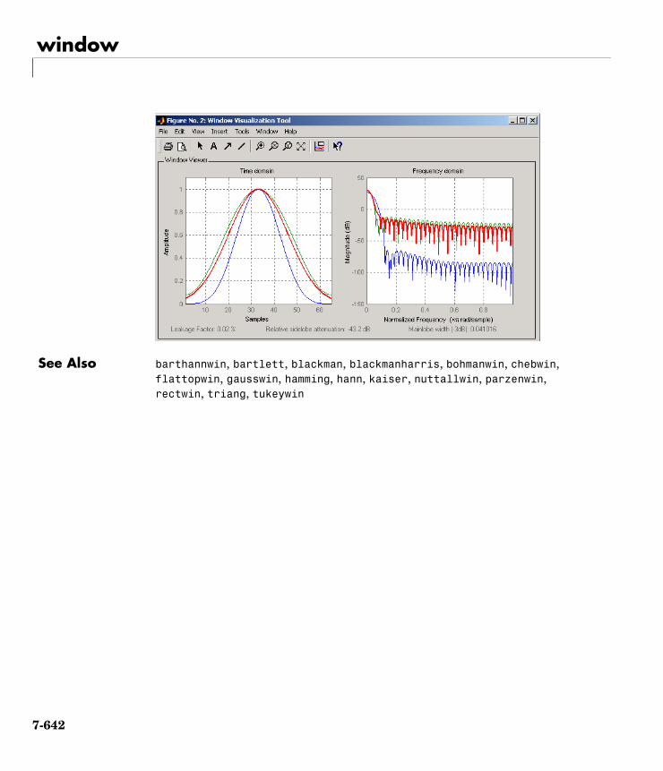
window
See Also barthannwin, bartlett, blackman, blackmanharris, bohmanwin, chebwin, flattopwin, gausswin, hamming, hann, kaiser, nuttallwin, parzenwin, rectwin, triang, tukeywin
7-642
wintool
7wintoolPurpose Open the Window Design and Analysis Tool (WinTool)
Syntax wintoolwintool(obj1,obj2,...)
Description wintool opens WinTool, a graphical user interface (GUI) for designing and analyzing spectral windows. It opens with a default 64-point Hamming window.
wintool(obj1,obj2,...) opens WinTool with the sigwin window object(s) specified in obj1, obj2, etc.
Note A related tool, wvtool, is available for displaying, annotating, or printing windows.
7-643
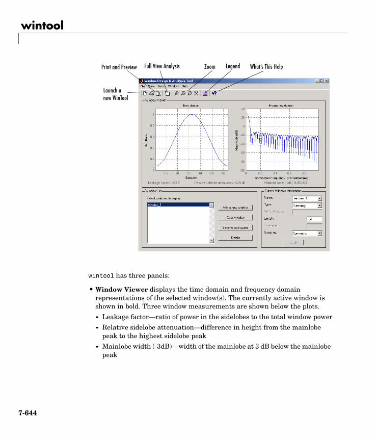
wintool
wintool has three panels:
• Window Viewer displays the time domain and frequency domain representations of the selected window(s). The currently active window is shown in bold. Three window measurements are shown below the plots.
- Leakage factor—ratio of power in the sidelobes to the total window power
- Relative sidelobe attenuation—difference in height from the mainlobe peak to the highest sidelobe peak
- Mainlobe width (-3dB)—width of the mainlobe at 3 dB below the mainlobe peak
Legend What’s This HelpZoom
Launch a new WinTool
Print and Preview Full View Analysis
7-644

wintool
• Window List lists the windows available for display in the Window Viewer. Highlight one or more windows to display them. The Window List buttons are:
- Add a new window—adds a default Hamming window with length 64 and symmetric sampling. You can change the information for this window by applying changes made in the Current Window Information panel.
- Copy window—copies the selected window(s).
- Save to workspace—saves the selected window(s) as vector(s) to the MATLAB workspace. The name of the window in wintool is used as the vector name.
- Delete—removes the selected window(s) from the window list.
• Current Window Information displays information about the currently active window. The active window name is shown in the Name field. To make another window active, select its name from the Name menu.
Window ParametersEach window is defined by the parameters in the Current Window Information panel. You can change the current window’s characteristics by changing its parameters and clicking Apply. The parameters of the current window are
- Name—name of the window. The name is used for the legend in the Window Viewer, in the Window List, and for the vector saved to the workspace. You can either select a name from the menu or type the desired name in the edit box.
- Type—algorithm for the window. Select the type from the menu. All windows in the Signal Processing Toolbox are available.
- MATLAB code—any valid MATLAB expression that returns a vector defining the window if Type = User Defined.
- Length—number of samples.
- Parameter—additional parameter for windows that require it, such as Chebyshev, which requires you to specify the sidelobe attenuation. Note that the title “Parameter” changes to the appropriate parameter name.
- Sampling—type of sampling to use for generalized cosine windows (Hamming, Hann, and Blackman)—Periodic or Symmetric. Periodic
7-645
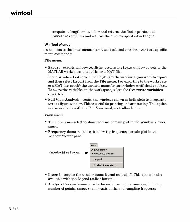
wintool
computes a length n+1 window and returns the first n points, and Symmetric computes and returns the n points specified in Length.
WinTool MenusIn addition to the usual menus items, wintool contains these wintool-specific menu commands:
File menu:
• Export—exports window coefficent vectors or sigwin window objects to the MATLAB workspace, a text file, or a MAT-file.
In the Window List in WinTool, highlight the window(s) you want to export and then select Export from the File menu. For exporting to the workspace or a MAT-file, specify the variable name for each window coefficient or object. To overwrite variables in the workspace, select the Overwrite variables check box.
• Full View Analysis—copies the windows shown in both plots to a separate wvtool figure window. This is useful for printing and annotating. This option is also available with the Full View Analysis toolbar button.
View menu:
• Time domain—select to show the time domain plot in the Window Viewer panel.
• Frequency domain—select to show the frequency domain plot in the Window Viewer panel.
• Legend—toggles the window name legend on and off. This option is also available with the Legend toolbar button.
• Analysis Parameters—controls the response plot parameters, including number of points, range, x- and y-axis units, and sampling frequency.
Checked plot(s) are displayed.
7-646
wintool
You can also access the Analysis Parameters by right-clicking on the x-axis label of a plot in the Window Viewer panel. The X-axis units for the time domain plot depend on the selected Sampling Frequency units.
Tools menu:
• Zoom In—zooms in along both x- and y-axes.
• Zoom X—zooms in along the x-axis only. Drag the mouse in the x direction to select the zoom area.
• Zoom Y—zooms in along the y-axis only. Drag the mouse in the y direction to select the zoom area.
• Full View—returns to full view.
See Also window, wvtool
Frequency Domain Time Domain
Hz sec
kHz ms
MHz µs
GHz picosec
7-647
wvtool
7wvtoolPurpose Open the Window Visualization Tool (WVTool)
Syntax wvtool(winname(n))wvtool(winname1(n),winname2(n),...winnamem(n))h = wvtool(...)
Description wvtool(winname(n)) opens WVTool with the time and frequency domain plots of the n-length window specified in winname, which can be any window in the Signal Processing Toolbox. For a list of valid window names, see the window function. In the wvtool command, do not precede the window name with @.
wvtool(winname1(n),winname2(n),...winnamem(n)) opens WVTool with a time-domain plot and a frequency-domain plot that contain all the windows specified in winname1,...winnamem. The plots are shown on the same axes so that window characteristics can be compared and contrasted easily. WVTool is useful for displaying, annotating, and printing window responses.
h = wvtool(...) returns the Handle Graphics figure handle h.
Note A related tool, wintool, is available for designing and analyzing windows.
7-648
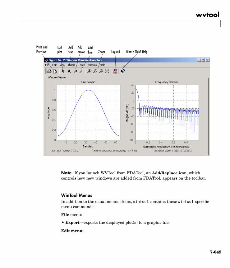
wvtool
Note If you launch WVTool from FDATool, an Add/Replace icon, which controls how new windows are added from FDATool, appears on the toolbar.
WinTool MenusIn addition to the usual menus items, wintool contains these wintool-specific menu commands:
File menu:
• Export—exports the displayed plot(s) to a graphic file.
Edit menu:
Legend What’s This? HelpZoomPrint and Preview
Edit plot
Add text
Add arrow
Add line
7-649
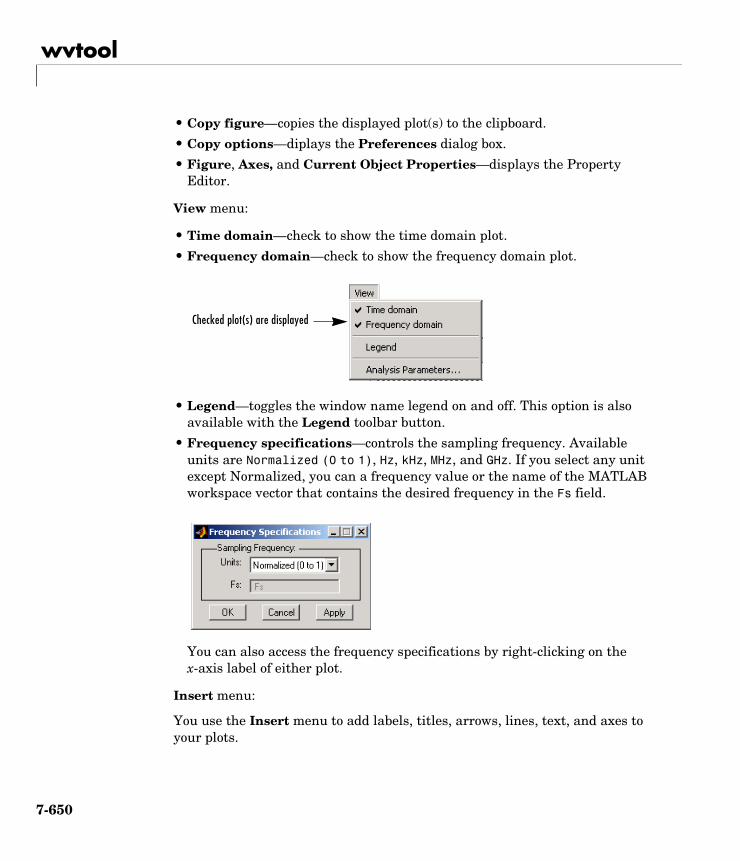
wvtool
• Copy figure—copies the displayed plot(s) to the clipboard.
• Copy options—diplays the Preferences dialog box.
• Figure, Axes, and Current Object Properties—displays the Property Editor.
View menu:
• Time domain—check to show the time domain plot.
• Frequency domain—check to show the frequency domain plot.
• Legend—toggles the window name legend on and off. This option is also available with the Legend toolbar button.
• Frequency specifications—controls the sampling frequency. Available units are Normalized (0 to 1), Hz, kHz, MHz, and GHz. If you select any unit except Normalized, you can a frequency value or the name of the MATLAB workspace vector that contains the desired frequency in the Fs field.
You can also access the frequency specifications by right-clicking on the x-axis label of either plot.
Insert menu:
You use the Insert menu to add labels, titles, arrows, lines, text, and axes to your plots.
Checked plot(s) are displayed
7-650
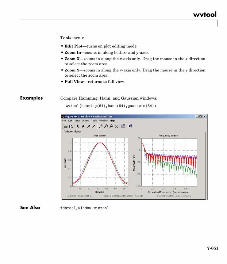
wvtool
Tools menu:
• Edit Plot—turns on plot editing mode
• Zoom In—zooms in along both x- and y-axes.
• Zoom X—zooms in along the x-axis only. Drag the mouse in the x direction to select the zoom area.
• Zoom Y—zooms in along the y-axis only. Drag the mouse in the y direction to select the zoom area.
• Full View—returns to full view.
Examples Compare Hamming, Hann, and Gaussian windows:
wvtool(hamming(64),hann(64),gausswin(64))
See Also fdatool, window, wintool
7-651
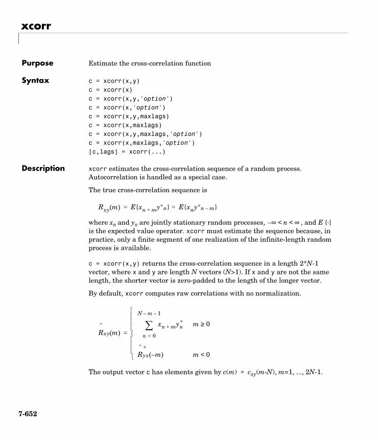
xcorr
7xcorrPurpose Estimate the cross-correlation function
Syntax c = xcorr(x,y)c = xcorr(x)c = xcorr(x,y,'option')c = xcorr(x,'option')c = xcorr(x,y,maxlags)c = xcorr(x,maxlags)c = xcorr(x,y,maxlags,'option')c = xcorr(x,maxlags,'option')[c,lags] = xcorr(...)
Description xcorr estimates the cross-correlation sequence of a random process. Autocorrelation is handled as a special case.
The true cross-correlation sequence is
where xn and yn are jointly stationary random processes, , and E · is the expected value operator. xcorr must estimate the sequence because, in practice, only a finite segment of one realization of the infinite-length random process is available.
c = xcorr(x,y) returns the cross-correlation sequence in a length 2*N-1 vector, where x and y are length N vectors (N>1). If x and y are not the same length, the shorter vector is zero-padded to the length of the longer vector.
By default, xcorr computes raw correlations with no normalization.
The output vector c has elements given by c(m) = cxy(m-N), m=1, ..., 2N-1.
Rxy m( ) Exn m+ y*n Exny*n m– ==
∞– n ∞< <
Rˆ
xy m( )xn m+ yn
*
n 0=
N m– 1–
∑ m 0≥
Rˆ
yx*
m–( ) m 0<
=
7-652
xcorr
In general, the correlation function requires normalization to produce an accurate estimate (see below).
c = xcorr(x) is the autocorrelation sequence for the vector x. If x is an N-by-P matrix, c is a matrix with 2N-1 rows whose P2 columns contain the cross-correlation sequences for all combinations of the columns of x. For more information on matrix processing with xcorr, see “Multiple Channels” on page 3-4.
c = xcorr(x,y,'option') specifies a normalization option for the cross-correlation, where 'option' is
• 'biased': Biased estimate of the cross-correlation function
• 'unbiased': Unbiased estimate of the cross-correlation function
• 'coeff': Normalizes the sequence so the autocorrelations at zero lag are identically 1.0.
• 'none', to use the raw, unscaled cross-correlations (default)
See reference [1] for more information on the properties of biased and unbiased correlation estimates.
c = xcorr(x,'option') specifies one of the above normalization options for the autocorrelation.
c = xcorr(x,y,maxlags) returns the cross-correlation sequence over the lag range [-maxlags:maxlags]. Output c has length 2*maxlags+1.
c = xcorr(x,maxlags) returns the autocorrelation sequence over the lag range [-maxlags:maxlags]. Output c has length 2*maxlags+1. If x is an N-by-P matrix, c is a matrix with 2*maxlags+1 rows whose P2 columns contain the autocorrelation sequences for all combinations of the columns of x.
c = xcorr(x,y,maxlags,'option') specifies both a maximum number of lags and a scaling option for the cross-correlation.
cxy biased, m( )1N----cxy m( )=
cxy unbiased, m( )1
N m–-------------------cxy m( )=
7-653
xcorr
c = xcorr(x,maxlags,'option') specifies both a maximum number of lags and a scaling option for the autocorrelation.
[c,lags] = xcorr(...) returns a vector of the lag indices at which c was estimated, with the range [-maxlags:maxlags]. When maxlags is not specified, the range of lags is [-N+1:N-1].
In all cases, the cross-correlation or autocorrelation computed by xcorr has the zeroth lag in the middle of the sequence, at element or row maxlags+1 (element or row N if maxlags is not specified).
Examples The second output, lags, is useful for plotting the cross-correlation or autocorrelation. For example, the estimated autocorrelation of zero-mean Gaussian white noise cww(m) can be displayed for -10 ≤ m ≤ 10 using:
ww = randn(1000,1);[c_ww,lags] = xcorr(ww,10,'coeff');stem(lags,c_ww)
Swapping the x and y input arguments reverses (and conjugates) the output correlation sequence. For row vectors, the resulting sequences are reversed left to right; for column vectors, up and down. The following example illustrates this property (mat2str is used for a compact display of complex numbers):
x = [1,2i,3]; y = [4,5,6];[c1,lags] = xcorr(x,y);c1 = mat2str(c1,2), lagsc1 =
[6-i*8.9e-016 5+i*12 22+i*10 15+i*8 12+i*8.9e-016]lags = -2 -1 0 1 2c2 = conj(fliplr(xcorr(y,x)));c2 = mat2str(c2,2)c2 =
[6-i*8.9e-016 5+i*12 22+i*10 15+i*8 12+i*8.9e-016]
For the case where input argument x is a matrix, the output columns are arranged so that extracting a row and rearranging it into a square array produces the cross-correlation matrix corresponding to the lag of the chosen row. For example, the cross-correlation at zero lag can be retrieved by:
randn('state',0)
7-654
xcorr
X = randn(2,2);[M,P] = size(X);c = xcorr(X);c0 = zeros(P); c0(:) = c(M,:) % Extract zero-lag row
c0 = 2.9613 -0.5334 -0.5334 0.0985
You can calculate the matrix of correlation coefficients that the MATLAB function corrcoef generates by substituting:
c = xcov(X,'coef')
in the last example. The function xcov subtracts the mean and then calls xcorr.
Use fftshift to move the second half of the sequence starting at the zeroth lag to the front of the sequence. fftshift swaps the first and second halves of a sequence.
Algorithm For more information on estimating covariance and correlation functions, see [1].
See Also conv, corrcoef, cov, xcorr2, xcov
References [1] Orfanidis, S.J., Optimum Signal Processing. An Introduction. 2nd Edition, Prentice-Hall, Englewood Cliffs, NJ, 1996.
7-655

xcorr2
7xcorr2Purpose Estimate the two-dimensional cross-correlation
Syntax C = xcorr2(A)C = xcorr2(A,B)
Description C = xcorr2(A,B) returns the cross-correlation of matrices A and B with no scaling. xcorr2 is the two-dimensional version of xcorr. It has its maximum value when the two matrices are aligned so that they are shaped as similarly as possible.
xcorr2(A) is the autocorrelation matrix of input matrix A. It is identical to xcorr2(A,A).
See Also conv2, filter2, xcorr
7-656
xcov
7xcovPurpose Estimate the cross-covariance function (mean-removed cross-correlation)
Syntax v = xcov(x,y)v = xcov(x)v = xcov(x,'option')[c,lags] = xcov(x,y,maxlags)[c,lags] = xcov(x,maxlags)[c,lags] = xcov(x,y,maxlags,'option')
Description xcov estimates the cross-covariance sequence of random processes. Autocovariance is handled as a special case.
The true cross-covariance sequence is the cross-correlation of mean-removed sequences
where and are the mean values of the two stationary random processes, and E· is the expected value operator. xcov estimates the sequence because, in practice, access is available to only a finite segment of the infinite-length random process.
v = xcov(x,y) returns the cross-covariance sequence in a length 2N-1 vector, where x and y are length N vectors. For information on how arrays are processed with xcov, see “Multiple Channels” on page 3-4.
v = xcov(x) is the autocovariance sequence for the vector x. Where x is an N-by-P array, v = xcov(x) returns an array with 2N-1 rows whose P2 columns contain the cross-covariance sequences for all combinations of the columns of x.
By default, xcov computes raw covariances with no normalization. For a length N vector
φxy µ( ) E xn m+ µx–( ) yn µy–( )* =
µx µy
cxy m( )x n m+( )
1N---- xi
i 0=
N 1–
∑–
yn* 1
N---- yi
*
i 0=
N 1–
∑–
n 0=
N m– 1–
∑ m 0≥
cyx* m–( ) m 0<
=
7-657
xcov
The output vector c has elements given by c(m) = cxy(m-N), m = 1, ..., 2N-1.
The covariance function requires normalization to estimate the function properly.
v = xcov(x,'option') specifies a scaling option, where 'option' is
• 'biased', for biased estimates of the cross-covariance function
• 'unbiased', for unbiased estimates of the cross-covariance function
• 'coeff', to normalize the sequence so the auto-covariances at zero lag are identically 1.0
• 'none', to use the raw, unscaled cross-covariances (default)
See [1] for more information on the properties of biased and unbiased correlation and covariance estimates.
[c,lags] = xcov(x,y,maxlags) where x and y are length m vectors, returns the cross-covariance sequence in a length 2*maxlags+1 vector c. lags is a vector of the lag indices where c was estimated, that is, [-maxlags:maxlags].
[c,lags] = xcov(x,maxlags) is the autocovariance sequence over the range of lags [-maxlags:maxlags].
[c,lags] = xcov(x,maxlags) where x is an m-by-p array, returns array c with 2*maxlags+1 rows whose P2 columns contain the cross-covariance sequences for all combinations of the columns of x.
[c,lags] = xcov(x,y,maxlags,'option') specifies a scaling option, where 'option' is the last input argument.
In all cases, xcov gives an output such that the zeroth lag of the covariance vector is in the middle of the sequence, at element or row maxlag+1 or at m.
Examples The second output lags is useful when plotting. For example, the estimated autocovariance of uniform white noise cww(m) can be displayed for -10 ≤ m ≤ 10 using:
ww = randn(1000,1); % Generate uniform noise with mean = 1/2.[cov_ww,lags] = xcov(ww,10,'coeff');stem(lags,cov_ww)
7-658
xcov
Algorithm xcov computes the mean of its inputs, subtracts the mean, and then calls xcorr. For more information on estimating covariance and correlation functions, see [1].
Diagnostics xcov does not check for any errors other than the correct number of input arguments. Instead, it relies on the error checking in xcorr.
See Also conv, corrcoef, cov, xcorr, xcorr2
References [1] Orfanidis, S.J., Optimum Signal Processing. An Introduction. 2nd Edition, Prentice-Hall, Englewood Cliffs, NJ, 1996.
7-659
yulewalk
7yulewalkPurpose Recursive digital filter design
Syntax [b,a] = yulewalk(n,f,m)
Description yulewalk designs recursive IIR digital filters using a least-squares fit to a specified frequency response.
[b,a] = yulewalk(n,f,m) returns row vectors b and a containing the n+1 coefficients of the order n IIR filter whose frequency-magnitude characteristics approximately match those given in vectors f and m:
• f is a vector of frequency points, specified in the range between 0 and 1, where 1 corresponds to half the sample frequency (the Nyquist frequency). The first point of f must be 0 and the last point 1, with all intermediate points in increasing order. Duplicate frequency points are allowed, corresponding to steps in the frequency response.
• m is a vector containing the desired magnitude response at the points specified in f.
• f and m must be the same length.
• plot(f,m) displays the filter shape.
The output filter coefficients are ordered in descending powers of z.
When specifying the frequency response, avoid excessively sharp transitions from passband to stopband. You may need to experiment with the slope of the transition region to get the best filter design.
Examples Design an 8th-order lowpass filter and overplot the desired frequency response with the actual frequency response:
f = [0 0.6 0.6 1];m = [1 1 0 0];[b,a] = yulewalk(8,f,m);[h,w] = freqz(b,a,128);plot(f,m,w/pi,abs(h),'--')legend('Ideal','yulewalk Designed')title('Comparison of Frequency Response Magnitudes')
B z( )A z( )----------- b 1( ) b 2( )z 1– b n 1+( )z n–+ + +
a 1( ) a 2( )z 1– a n 1+( )z n–+ + +-------------------------------------------------------------------------------------=
7-660
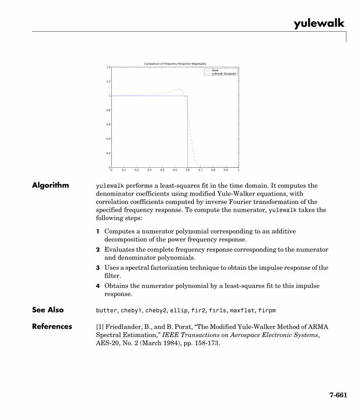
yulewalk
Algorithm yulewalk performs a least-squares fit in the time domain. It computes the denominator coefficients using modified Yule-Walker equations, with correlation coefficients computed by inverse Fourier transformation of the specified frequency response. To compute the numerator, yulewalk takes the following steps:
1 Computes a numerator polynomial corresponding to an additive decomposition of the power frequency response.
2 Evaluates the complete frequency response corresponding to the numerator and denominator polynomials.
3 Uses a spectral factorization technique to obtain the impulse response of the filter.
4 Obtains the numerator polynomial by a least-squares fit to this impulse response.
See Also butter, cheby1, cheby2, ellip, fir2, firls, maxflat, firpm
References [1] Friedlander, B., and B. Porat, “The Modified Yule-Walker Method of ARMA Spectral Estimation,” IEEE Transactions on Aerospace Electronic Systems, AES-20, No. 2 (March 1984), pp. 158-173.
0 0.1 0.2 0.3 0.4 0.5 0.6 0.7 0.8 0.9 10
0.2
0.4
0.6
0.8
1
1.2
1.4Comparison of Frequency Response Magnitudes
Ideal yulewalk Designed
7-661
zerophase
7zerophasePurpose Return the zero-phase response of a real filter
Syntax [Hr,w] = zerophase(b,a)[Hr,w] = zerophase(b,a,nfft)[Hr,w] = zerophase(b,a,nfft,'whole')[Hr,w] = zerophase(b,a,w)[Hr,f] = zerophase(...,fs)[Hr,w,phi] = zerophase(...)zerophase(...)
Description [Hr,w] = zerophase(b,a) returns the zero-phase response Hr, and the frequency vector w (in radians/sample) at which Hr is computed, given a filter defined by numerator b and denominator a. For FIR filters where a=1, you can omit the value a from the command. The zero-phase response is evaluated at 512 equally spaced points on the upper half of the unit circle.
The zero-phase response, Hr(w), is related to the frequency response, H(w) by
,
where is the frequency response, Hr(ω) is the zero-phase response and ϕ(w) is the continuous phase.
Note The zero-phase response is always real, but it is not the equivalent of the magnitude response. The former can be negative while the latter cannot be negative.
[Hr,w] = zerophase(b,a,nfft) returns the zero-phase response Hr and frequency vector w (radians/sample), using nfft frequency points on the upper half of the unit circle.
[Hr,w] = zerophase(b,a,nfft,'whole') returns the zero-phase response Hr and frequency vector w (radians/sample), using nfft frequency points around the whole unit circle.
[Hr,w] = zerophase(b,a,w) returns the zero-phase response Hr and frequency vector w (radians/sample) at frequencies in vector w.
H ejω( ) Hr ω( ) ejϕ ω( )=
H ejω( )
7-662
zerophase
[Hr,f] = zerophase(...,fs) returns the zero-phase response Hr and frequency vector f (Hz), using the sampling frequency fs (in Hz), to determine the frequency vector f (in Hz) at which Hr is computed.
[Hr,w,phi] = zerophase(...) returns the zero-phase response Hr, frequency vector w (rad/sample), and the continuous phase component, phi. (Note that this quantity is not equivalent to the phase response of the filter when the zero-phase response is negative.)
zerophase(...) with no output arguments, plots the zero-phase response versus frequency.
Examples Example 1Plot the zero-phase response of a constrained least squares FIR filter:
b=fircls1(54,.3,.02,.008);zerophase(b);
Example 2Plot the zero-phase response of an elliptic filter:
[b,a]=ellip(10,.5,20,.4;zerophase(b,a,512,'whole');
See Also freqs, freqz, fvtool, grpdelay, invfreqz, phasedelay, phasez
7-663
zp2sos
7zp2sosPurpose Convert digital filter zero-pole-gain parameters to second-order sections form
Syntax [sos,g] = zp2sos(z,p,k)[sos,g] = zp2sos(z,p,k,'order')[sos,g] = zp2sos(z,p,k,'order','scale')sos = zp2sos(...)
Description zp2sos converts a discrete-time zero-pole-gain representation of a given digital filter to an equivalent second-order section representation.
Use [sos,g] = zp2sos(z,p,k) to obtain a matrix sos in second-order section form with gain g equivalent to the discrete-time zero-pole-gain filter represented by input arguments z, p, and k. Vectors z and p contain the zeros and poles of the filter’s transfer function H(z), not necessarily in any particular order.
where n and m are the lengths of z and p, respectively, and k is a scalar gain. The zeros and poles must be real or complex conjugate pairs. sos is an L-by-6 matrix
whose rows contain the numerator and denominator coefficients bik and aik of the second-order sections of H(z).
The number L of rows of the matrix sos is the closest integer greater than or equal to the maximum of n/2 and m/2.
H z( ) kz z1–( ) z z2–( ) z zn–( )z p1–( ) z p2–( ) z pm–( )
--------------------------------------------------------------------=
sos
b01 b11 b21 1 a11 a21
b02 b12 b22 1 a12 a22
b0L b1L b2L 1 a1L a2L
=
H z( ) g Hk z( )
k 1=
L
∏ gb0k b1kz 1– b2kz 2–+ +
1 a1kz 1– a2kz 2–+ +----------------------------------------------------------
k 1=
L
∏= =
7-664
zp2sos
[sos,g] = zp2sos(z,p,k,'order') specifies the order of the rows in sos, where 'order' is
• 'down', to order the sections so the first row of sos contains the poles closest to the unit circle
• 'up', to order the sections so the first row of sos contains the poles farthest from the unit circle (default)
[sos,g] = zp2sos(z,p,k,'order','scale') specifies the desired scaling of the gain and the numerator coefficients of all second-order sections, where 'scale' is
• 'none', to apply no scaling (default)
• 'inf', to apply infinity-norm scaling
• 'two', to apply 2-norm scaling
Using infinity-norm scaling in conjunction with up-ordering minimizes the probability of overflow in the realization. Using 2-norm scaling in conjunction with down-ordering minimizes the peak round-off noise.
Note Infinity-norm and 2-norm scaling are appropriate only for direct-form II implementations.
sos = zp2sos(...) embeds the overall system gain, g, in the first section, H1(z), so that
Note Embedding the gain in the first section when scaling a direct-form II structure is not recommended and may result in erratic scaling. To avoid embedding the gain, use ss2sos with two outputs.
H z( ) Hk z( )
k 1=
L
∏=
7-665
zp2sos
Examples Find a second-order section form of a Butterworth lowpass filter:
[z,p,k] = butter(5,0.2);sos = zp2sos(z,p,k);
Algorithm zp2sos uses a four-step algorithm to determine the second-order section representation for an input zero-pole-gain system:
1 It groups the zeros and poles into complex conjugate pairs using the cplxpair function.
2 It forms the second-order section by matching the pole and zero pairs according to the following rules:
a Match the poles closest to the unit circle with the zeros closest to those poles.
b Match the poles next closest to the unit circle with the zeros closest to those poles.
c Continue until all of the poles and zeros are matched.
zp2sos groups real poles into sections with the real poles closest to them in absolute value. The same rule holds for real zeros.
3 It orders the sections according to the proximity of the pole pairs to the unit circle. zp2sos normally orders the sections with poles closest to the unit circle last in the cascade. You can tell zp2sos to order the sections in the reverse order by specifying the down flag.
4 zp2sos scales the sections by the norm specified in the 'scale' argument. For arbitrary H(ω), the scaling is defined by
where p can be either ∞ or 2. See the references for details on the scaling. This scaling is an attempt to minimize overflow or peak round-off noise in fixed point filter implementations.
See Also cplxpair, filternorm, sos2zp, ss2sos, tf2sos, zp2ss, zp2tf
H p1
2π------ H ω( ) p ωd
0
2π
∫
1p---
=
7-666

zp2sos
References [1] Jackson, L.B., Digital Filters and Signal Processing, 3rd ed., Kluwer Academic Publishers, Boston, 1996, Chapter 11.
[2] Mitra, S.K., Digital Signal Processing: A Computer-Based Approach, McGraw-Hill, New York, 1998, Chapter 9.
[3] Vaidyanathan, P.P., “Robust Digital Filter Structures,” Handbook for Digital Signal Processing, S.K. Mitra and J.F. Kaiser, ed., John Wiley & Sons, New York, 1993, Chapter 7.
7-667
zp2ss
7zp2ssPurpose Convert zero-pole-gain filter parameters to state-space form
Syntax [A,B,C,D] = zp2ss(z,p,k)
Description zp2ss converts a zero-pole-gain representation of a given system to an equivalent state-space representation.
[A,B,C,D] = zp2ss(z,p,k) finds a single input, multiple output, state-space representation
given a system in factored transfer function form.
Column vector p specifies the pole locations, and matrix z the zero locations with as many columns as there are outputs. The gains for each numerator transfer function are in vector k. The A, B, C, and D matrices are returned in controller canonical form.
Inf values may be used as place holders in z if some columns have fewer zeros than others.
Algorithm zp2ss, for single-input systems, groups complex pairs together into two-by-two blocks down the diagonal of the A matrix. This requires the zeros and poles to be real or complex conjugate pairs.
See Also sos2ss, ss2zp, tf2ss, zp2sos, zp2tf
x· Ax Bu+=
y Cx Du+=
H s( )Z s( )P s( )---------- k
s z1–( ) s z2–( ) s zn–( )s p1–( ) s p2–( ) s pn–( )
------------------------------------------------------------------= =
7-668
zp2tf
7zp2tfPurpose Convert zero-pole-gain filter parameters to transfer function form
Syntax [b,a] = zp2tf(z,p,k)
Description zp2tf forms transfer function polynomials from the zeros, poles, and gains of a system in factored form.
[b,a] = zp2tf(z,p,k) finds a rational transfer function
given a system in factored transfer function form
Column vector p specifies the pole locations, and matrix z specifies the zero locations, with as many columns as there are outputs. The gains for each numerator transfer function are in vector k. The zeros and poles must be real or come in complex conjugate pairs. The polynomial denominator coefficients are returned in row vector a and the polynomial numerator coefficients are returned in matrix b, which has as many rows as there are columns of z.
Inf values can be used as place holders in z if some columns have fewer zeros than others.
Algorithm The system is converted to transfer function form using poly with p and the columns of z.
See Also sos2tf, ss2tf, tf2zp, tf2zpk, zp2sos, zp2ss
B s( )A s( )-----------
b1s n 1–( ) b n 1–( )s bn+ + +
a1s m 1–( ) a m 1–( )s am+ + +--------------------------------------------------------------------------------=
H s( )Z s( )P s( )---------- k
s z1–( ) s z2–( ) s zm–( )s p1–( ) s p2–( ) s pn–( )
------------------------------------------------------------------= =
7-669
zplane
7zplanePurpose Zero-pole plot
Syntax zplane(z,p)zplane(b,a)zplane(Hd)[hz,hp,ht] = zplane(z,p)
Description This function displays the poles and zeros of discrete-time systems.
zplane(z,p) plots the zeros specified in column vector z and the poles specified in column vector p in the current figure window. The symbol 'o' represents a zero and the symbol 'x' represents a pole. The plot includes the unit circle for reference. If z and p are arrays, zplane plots the poles and zeros in the columns of z and p in different colors.
You can override the automatic scaling of zplane using
axis([xmin xmax ymin ymax])
or
set(gca,'ylim',[ymin ymax])
or
set(gca,'xlim',[xmin xmax])
after calling zplane. This is useful in the case where one or a few of the zeros or poles have such a large magnitude that the others are grouped tightly around the origin and are hard to distinguish.
zplane(b,a) where b and a are row vectors, first uses roots to find the zeros and poles of the transfer function represented by numerator coefficients b and denominator coefficients a.
zplane(Hd) finds the zeros and poles of the transfer function represented by the dfilt filter object Hd. The pole-zero plot is displayed in fvtool.
[hz,hp,ht] = zplane(z,p) returns vectors of handles to the zero lines, hz, and the pole lines, hp. ht is a vector of handles to the axes/unit circle line and to text objects, which are present when there are multiple zeros or poles. If there are no zeros or no poles, hz or hp is the empty matrix [].
7-670
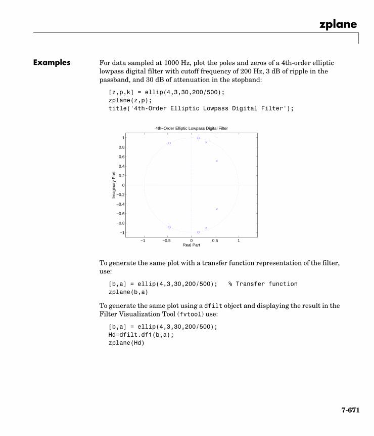
zplane
Examples For data sampled at 1000 Hz, plot the poles and zeros of a 4th-order elliptic lowpass digital filter with cutoff frequency of 200 Hz, 3 dB of ripple in the passband, and 30 dB of attenuation in the stopband:
[z,p,k] = ellip(4,3,30,200/500);zplane(z,p);title('4th-Order Elliptic Lowpass Digital Filter');
To generate the same plot with a transfer function representation of the filter, use:
[b,a] = ellip(4,3,30,200/500); % Transfer functionzplane(b,a)
To generate the same plot using a dfilt object and displaying the result in the Filter Visualization Tool (fvtool) use:
[b,a] = ellip(4,3,30,200/500);Hd=dfilt.df1(b,a);zplane(Hd)
−1 −0.5 0 0.5 1
−1
−0.8
−0.6
−0.4
−0.2
0
0.2
0.4
0.6
0.8
1
Real Part
Imag
inar
y P
art
4th−Order Elliptic Lowpass Digital Filter
7-671
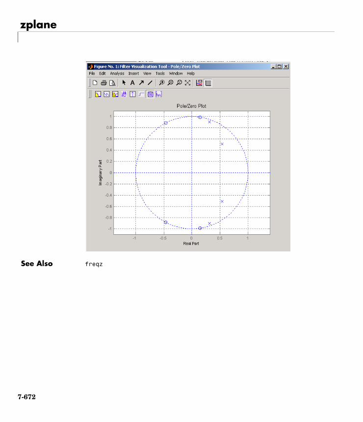
zplane
See Also freqz
7-672

A
Technical Conventions
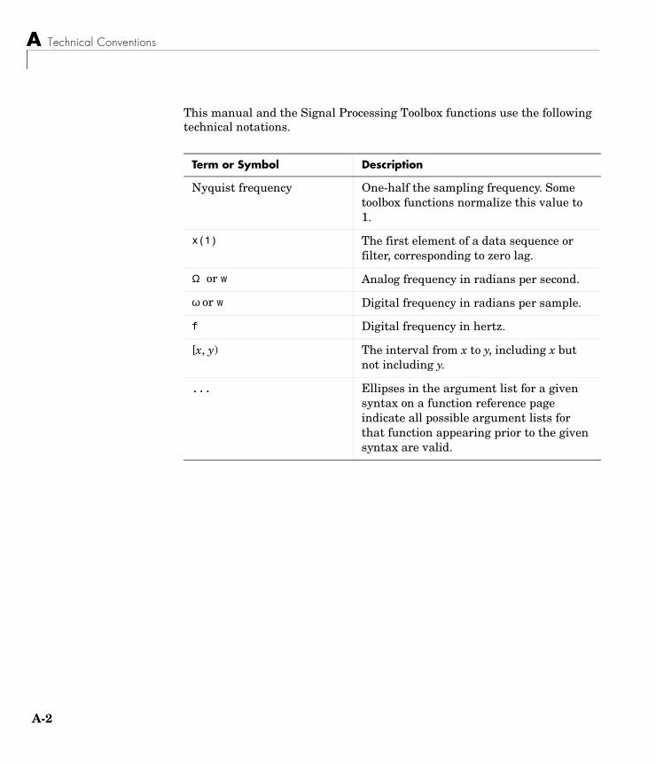
A Technical Conventions
A-2
This manual and the Signal Processing Toolbox functions use the following technical notations.
Term or Symbol Description
Nyquist frequency One-half the sampling frequency. Some toolbox functions normalize this value to 1.
x(1) The first element of a data sequence or filter, corresponding to zero lag.
Ω or w Analog frequency in radians per second.
ω or w Digital frequency in radians per sample.
f Digital frequency in hertz.
[x, y) The interval from x to y, including x but not including y.
... Ellipses in the argument list for a given syntax on a function reference page indicate all possible argument lists for that function appearing prior to the given syntax are valid.
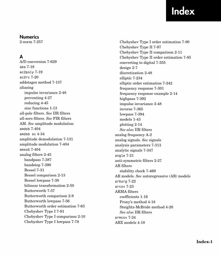
Index
Numerics2-norm 7-257
AA/D conversion 7-629abs 7-18ac2poly 7-19ac2rc 7-20addstages method 7-137aliasing
impulse invariance 2-48preventing 4-27reducing 4-45sinc functions 1-13
all-pole filters. See IIR filtersall-zero filters. See FIR filtersAM. See amplitude modulationamdsb 7-404amdsb sc 4-34amplitude demodulation 7-131amplitude modulation 7-404amssb 7-404analog filters 2-45
bandpass 7-387bandstop 7-390Bessel 7-31Bessel comparison 2-13Bessel lowpass 7-30bilinear transformation 2-50Butterworth 7-57Butterworth comparison 2-9Butterworth lowpass 7-56Butterworth order estimation 7-63Chebyshev Type I 7-91Chebyshev Type I comparison 2-10Chebyshev Type I lowpass 7-78
Chebyshev Type I order estimation 7-80Chebyshev Type II 7-97Chebyshev Type II comparison 2-11Chebyshev Type II order estimation 7-85converting to digital 7-355design 2-7discretization 2-48elliptic 7-234elliptic order estimation 7-242frequency response 7-301frequency response example 2-14highpass 7-392impulse invariance 2-48inverse 7-365lowpass 7-394models 1-43plotting 2-14See also IIR filters
analog frequency A-2analog signals. See signalsanalysis parameters 7-313analytic signals 7-347angle 7-21anti-symmetric filters 2-27AR filters
stability check 7-469AR models. See autoregressive (AR) modelsarburg 7-22arcov 7-23ARMA filters
coefficients 1-16Prony’s method 4-18Steiglitz-McBride method 4-20See also IIR filters
armcov 7-24ARX models 4-18
Index-1
Index
Ind
aryule 7-25ASCII files
importing 1-14autocorrelation 7-653
convert from LP coefficients 7-467convert from reflection coefficients 7-492convert to LP coefficients 7-19convert to reflection coefficients 7-20estimation 3-4multiple channel filters 3-4two-dimensional 7-656variance 3-4
autocovariance 7-657multiple channels 3-4
autoregressive (AR) modelsBurg method 7-22coefficients 1-16covariance method 7-23modified covariance method 7-24power spectral density (Burg method) 7-416power spectral density (covariance method)
7-422power spectral density (modified covariance
method) 7-447power spectral density (Yule-Walker method)
7-485Yule-Walker method 7-25See also IIR filters
autoregressive moving-average (ARMA) filters. See ARMA filters
avgpower method 7-212
ex-2
Bband edges
prewarping 2-51bandpass filters
Bessel 7-31Butterworth 7-57Chebyshev Type I 7-91Chebyshev Type I example 2-47Chebyshev Type II 7-96design 2-6elliptic 7-234FIR 2-22FIR example 7-266impulse invariance 2-49transform from lowpass 7-387
bandstop filtersBessel 7-31Butterworth 7-58Chebyshev Type I 7-92Chebyshev Type II 7-97elliptic 7-235FIR 7-265transform from lowpass 7-390
bandwidth 2-47barthannwin 7-26bartlett 7-28Bartlett windows
comparison 4-2Bartlett-Hann windows 7-26
comparison 4-2Bessel filters 7-31
characteristics 2-13limitations 7-33lowpass 7-30prototype 7-30
besselap 7-30besself 7-31
Index
bias 3-3linear prediction 4-17power spectral density 3-16variance trade-off 3-4Welch 3-23
bilinear 7-34bilinear transformations 7-34
characteristics 2-50output 7-35prewarping 7-34prewarping example 2-51
bit reversal 7-39bitrevorder 7-39blackman 7-41Blackman windows 7-41
comparison 4-2blackmanharris 7-43Blackman-Harris windows 7-43
comparison 4-2Nuttall 7-412
block method 7-137Bohman windows 7-45
comparison 4-2bohmanwin 7-45boxcar windows. See rectangular windowsbrackets A-2buffer 7-47Burg method
characteristics 3-36example 3-37spectral estimation 3-7Welch’s method comparison 3-38
Burg spectrum object 7-553buttap 7-56butter 7-57
Butterworth filters 7-57characteristics 2-9comparison 2-9generalized 2-15limitations 7-61lowpass 7-56order estimation 7-62
buttord 7-62
CC header file generation 5-35canonical forms 1-18
naming conventions 7-612carrier frequency 4-34carrier signals 4-34cascade method 7-137cascades 1-39Cauer filters. See elliptic filterscceps 7-67cell2sos 7-69center frequency 2-47centerdc method 7-212cepstrum
characteristics 4-28complex 4-28example 4-28inverse 4-30inverse function 7-496real 4-29reconstructing 4-30
cfirpm 7-70cheb1ap 7-78cheb1ord 7-79cheb2ap 7-83cheb2ord 7-84chebwin 7-89
Index-3
Index
Ind
cheby1 7-91cheby2 7-96Chebyshev error minimization 7-287Chebyshev Type I filters 7-91
characteristics 2-10example 2-47lowpass 7-78order estimation 7-79
Chebyshev Type II filters 7-96characteristics 2-11limitations 7-95order estimation 2-7
Chebyshev windows 7-89comparison 4-2
chirp 7-101chirp signals 1-10chirp z-transforms 7-122
characteristics 4-41coding
PCM 7-629coefficients
accessing filter 6-35convert autocorrelation to filter 7-19convert filter to autocorrelation 7-467convert filter to reflection 7-469convert reflection to autocorrelation 7-492convert reflection to filter 7-495filter 1-16lattice 1-39linear prediction 7-396reflection 7-20
coefficients method 7-137coherence 7-407
definition 3-29linearly dependent data 3-29
colorsSPTool 6-51
ex-4
communicationsapplications 4-34modeling 4-15simulation 7-131See also modulation, demodulation, voltage
controlled oscillationcompact disc
standards 4-26compaction
discrete cosine transform 4-44complex envelope. See Hilbert transformscontext-sensitive help 6-7continuous signals. See signalscontinuous-time filters. See analog filtersconv 7-107conv2 7-108conversions
autocorrelation to filter coefficients 7-19autocorrelation to reflection coefficients 7-20errors 5-24filter coefficients to autocorrelation 7-467filter coefficients to reflection coefficients 7-469functions (table) 1-44reflection coefficients to autocorrelation 7-492reflection coefficients to filter coefficients 7-495second-order section to zero-pole-gain 7-535second-order sections to state-space 7-531second-order sections to transfer functions
7-533state-space to second-order sections 7-589state-space to zero-pole-gain 7-594transfer functions to lattice 7-607transfer functions to second-order sections
7-608transfer functions to state-space 7-611zero-pole-gain to second-order sections 7-664zero-pole-gain to state-space 7-668
Index
convert method 7-137convmtx 7-109convolution
cross-correlation 3-2filtering 1-15matrix 1-42matrix function (convmtx) 7-109
corrcoef 7-111correlation
bias 3-3cross-correlation 7-652linear prediction 4-17matrices
covariance method 7-112modified covariance method 7-112
See also autocorrelation, cross-correlationcorrelation matrices 7-112corrmtx 7-112corrmtx 7-112cosine windows 4-7cov 7-115covariance
definition 3-8methods 3-41See also autocovariance, cross-covarianceSee also modified covariance method
covariance spectrum object 7-555, 7-563cplxpair 7-116cpsd 7-117cross power spectral density 7-117
definition 3-27cross spectral density
definition 3-27See also power spectral density, spectral
estimation
cross-correlation 7-652comparison to cross-covariance 3-2estimation bias 3-3filters, multiple channels 3-4normalization 3-4two-dimensional 7-656
cross-covariance 7-657comparison to cross-correlation 3-2multiple channels 3-4
cutoff frequencydefinition 7-31
czt 7-122czt. See chirp z-transforms
Ddata
markers 5-16multichannel matrix 1-5multichannel signals 1-8time vectors 1-7vectors 1-5
DC component suppression 1-48dct 7-125de la Valle-Poussin windowSee Parzen windowsdecimate 7-127decimation 7-127decode 7-626deconv 7-130deconvolution 4-40default session
SPTool 6-51delays
group 1-30noninteger 2-29phase 1-31signals 2-28
Index-5
Index
Ind
demod 7-131demod 7-131demodulation 7-131
example 4-35phase 7-132pulse position 7-132pulse width 7-132quadrature amplitude 7-132
dfilt 7-134cascade 7-147convert structures 7-144copying 7-144df1 7-149df1sos 7-152df1t 7-154df1tsos 7-156df2 7-158df2sos 7-161df2tsos 7-165direct-form antisymmetric FIR 7-167direct-form FIR transposed 7-173direct-form II transposed (df2t) 7-163direct-form IIR 7-171direct-form symmetric FIR 7-175FFT FIR 7-179filter implementation 2-53lattice allpass 7-181lattice ARMA 7-185lattice autoregressive 7-183lattice moving-average maximum 7-187lattice moving-average minimum 7-189methods 7-136parallel 7-191scalar 7-192state space 7-195structures 7-134
dfilt.cascade 7-147
ex-6
dfilt.df1 7-149dfilt.df1sos 7-152dfilt.df1t 7-154dfilt.df1tsos 7-156dfilt.df2 7-158dfilt.df2sos 7-161dfilt.df2t 7-163dfilt.df2tsos 7-165dfilt.dfasymfir 7-167dfilt.dffir 7-171dfilt.dffirt 7-173dfilt.dfsymfir 7-175dfilt.fftfir 7-179dfilt.latticeallpass 7-181dfilt.latticear 7-183dfilt.latticearma 7-185dfilt.latticemamax 7-187dfilt.latticemamin 7-189dfilt.parallel 7-191dfilt.scalar 7-192dfilt.statespace 7-195dft. See discrete Fourier transformsdftmtx 7-198difference equations 1-34differentiators
definition 2-29least square linear-phase FIR 7-283Parks-McClellan FIR 7-289
digit reversal 7-199digital audio tape standards 4-26digital filters
anti-causal 1-21Butterworth 7-57Butterworth order estimation 7-62cascade 1-39Chebyshev Type I order estimation
7-79
Index
Chebyshev Type II 7-96Chebyshev Type II order estimation 7-84coefficients 1-16comparison to IIR 2-17convolution 1-15convolution matrices 1-42design 2-2elliptic 7-234elliptic order estimation 7-241equiripple FIR order estimation 7-294FFT FIR overlap-add 7-251FIR design 2-17fixed-point implementation 1-39frequency response 1-26group delay 1-30, 7-339identification from frequency data 7-369IIR
comparison to FIR 2-4IIR design 2-4implementation with filter 1-15impulse response 7-357impulse response definition 1-24initial conditions 1-18lattice/ladder structures 1-39models 1-34order 1-16phase delay definition 1-31poles 1-35second-order sections 1-39specifications 2-7state-space 1-36time-domain representation 1-17transfer functions representation 1-16transients 1-23transposed direct-form II structures 1-18types 1-16zero-phase 7-259
zero-phase implementation 1-21zero-pole analysis 1-32zeros 1-35See also FIR filters, IIR filters
digital frequency A-2digitrevorder 7-199diric 7-201Dirichlet functions 7-201
definition 1-13discrete cosine transforms 7-125
definition 4-43example 4-44inverse 7-352reconstruct signals 4-44
discrete cosine transforms (DCT)energy compaction property 4-44
discrete Fourier transformsalgorithms 1-47definition 1-46eigenvector equivalent 3-43goertzel 1-48IIR filter implementation 1-23inverse two-dimensional 1-48magnitude 1-47matrix 7-198phase 1-47power spectrum estimation 3-9signal length dependencies 1-47spectral analysis 3-5time-dependent 4-32two-dimensional 1-48See also fast Fourier transforms (FFT), fft
discrete prolate spheroidal sequences See dpss
Index-7
Index
Ind
discretization 7-355bilinear transformations 2-50filters 2-48impulse invariance 2-48
dpssdpss.mat file 3-27example 3-27
dpss 7-204dpssclear 7-207dpssdir 7-208dpssload 7-209dpsssave 7-210dspdata
mean-square spectrum 7-217psd 7-222pseudospectrum 7-227
dspdata 7-211dspdata object 7-211dspdata.msspectrum 7-217dspdata.psd 7-222dspdata.pseudospectrum 7-227dspopts 7-232dspopts object 7-232duty cycles 1-9
Eecho detection 4-28edge effects 1-23eigenanalysis 3-43
frequency estimation 3-43eigenvector method 7-428
definition 3-42root MUSIC 7-508spectral estimation 3-7See also multiple signal classification method
Eigenvector spectrum object 7-557
ex-8
ellip 7-234ellipap 7-240ellipord 7-241elliptic filters 7-234
definition 2-12limitations 7-238order estimation 7-241
encoding 7-629eqtflength 7-246equiripple
Chebyshev Type I filters 2-10Chebyshev Type II filters 2-11Chebyshev windows 4-14elliptic filters 2-12elliptic filters (analog) 7-240elliptic filters (Cauer) 7-234Parks-McClellan design 7-287
equiripple filtersdefinition 2-23
error minimization 2-23weighted frequency bands 2-27
estimationcovariance method 7-23cross spectral density 3-27modified covariance method 7-24nonparametric 3-7parametric 3-7spectral density 3-7transfer functions 3-27Yule-Walker method 7-25See also parametric modeling
exportfilter 5-31window 7-646
Index
Ffast Fourier Transforms
Goertzel algorithm 7-333fast Fourier transforms 1-46
example 1-47frequency response 1-26implementation 1-23output 1-48
fcfwrite method 7-138FDATool
analysis buttons 5-15analysis functions 5-15computing coefficients 5-14design methods 5-9exporting filters 5-31filter architecture 5-24filter design specification 5-10filter implementation 5-24filter order specification 5-10filter realization 5-24filters structure 5-24frequency response specification 5-12group delay 5-15importing coefficients 5-27importing filters 5-27impulse response 5-15magnitude response 5-15M-files 5-38opening 5-7phase delay 5-15phase response 5-15pole-zero plots 5-15response type 5-8saving coefficients 5-31second analysis 5-15sessions 5-41step response 5-15
fdatool 7-247FFT. See fast Fourier transforms 1-23fftfilt 7-251fftshift 7-254filter
initial conditions 7-144overlap-add 7-179second-order sections 7-537states 7-144, 7-262
filter 1-18, 7-255filter coefficients
convert from reflection coefficients 7-495convert to reflection coefficients 7-469
filter design. See FDATool 5-2Filter Designer 6-11
edit 6-42filters
saving 6-34FIR methods 6-11IIR methods 6-11introduction 7-584redesign 6-50sample frequency 6-36spectra 6-12start 6-12types 6-11
filter method 7-138Filter Viewer
introduction 7-585open 6-14printing 6-28see FVTool 6-14
Filter Visualization Tool (FVTool) 7-308filter2 7-256filternorm 7-257filters
filter function 1-17
Index-9
Index
Ind
analog 2-9analog lowpass 7-30analog lowpass prototype 7-56anti-causal 1-21anti-symmetric 2-27bit reversal 7-39Butterworth 7-57Butterworth (generalized) 2-15Butterworth order 7-62C header file 5-35Chebyshev Type I 7-91Chebyshev Type I lowpass prototype 7-78Chebyshev Type I order 7-79Chebyshev Type II 7-96Chebyshev Type II order 7-84coefficients 1-16, 1-17coefficients in SPTool 6-35convert coefficients to autocorrelation 7-467convolution 1-15design 2-5, 6-11digit reversal 7-199discretization 2-48elliptic 7-234elliptic order 7-241equiripple 2-23export to MAT-file 5-33export to text file 5-33export to workspace 5-31filter and filtfilt comparison 1-21FIR 7-287FIR design 2-23FIR single band 2-22frequency data 7-365frequency domain 1-23frequency transformations 2-45fvtool 7-308Gaussian 7-277
ex-10
implementation 2-53importing to SPTool 6-40initial conditions 1-18, 7-260inverse analog 7-365inverse discrete-time 7-369lattice/ladder 1-39linear phase 2-18linear phase types 2-18linear prediction 4-17linear system models 1-34linear time-invariant digital 1-3median 4-33, 7-403minimax 2-23minimum phase 7-472name 5-17norm 7-257numerator and denominator length 7-246objects 7-134order 1-16overlap-add 7-251phase delay 7-440phase distortion removal 1-20phase modulation 4-30phase response 7-443pole-zero editor 5-20sampling frequency 5-17saving 5-39Savitzky-Golay 7-522Savitzky-Golay design 7-518Schur realizations 7-515second-order sections 1-39second-order sections IIR 7-537SPTool Filter Designer 6-11step response 7-596structures 2-53types 1-16viewing 7-308
Index
zero phase response 7-662zero-phase 7-259zero-phase implementation 1-21See also FDATool, FIR filters, IIR filters, digital
filters, analog filtersfiltfilt 7-259
filter comparison 1-21filtic 7-260, 7-262filtstates object 7-262FIR filters 2-17
arbitrary response 2-38complex response 7-70constrained least square 2-31differentiators 2-29equiripple 2-23example 6-21frequency domain 1-20, 1-23frequency response 7-268Gaussian 7-277Hilbert transformers 2-27IIR filter comparison 2-17implementation 1-18interpolation 7-363Kaiser windows 4-12lattice/ladder 1-39least square and equiripple comparison 2-24least square linear phase 7-282least square multiband 2-34least square weighted 2-36linear phase 2-18linear phase Parks-McClellan 7-287multiband 2-23multiband example 2-22nonlinear phase response 7-70order estimation 7-294overlap-add 7-251Parks-McClellan method 7-287
reduced delay response 2-41resample 1-20SPTool Filter Designer 6-11standard band 2-22types 7-292window-based 7-264windowing method 2-19
fir1
example 2-21fircls 7-271fircls1 7-274firgauss 7-277firls 7-282
cfirpm comparison 2-24differentiators 2-29weight vectors 2-27
firpm 2-17, 2-24, 7-287differentiators 2-29filter characteristics 7-292firls, comparison to 2-24Hilbert transformers 2-27order estimation 7-294weight vectors 2-27
firpmord 2-17, 7-294firrcos 7-297firtype method 7-138flattopwin 7-299FM. See frequency modulationfopen 1-14Fourier transforms. See discrete Fourier
transforms, fast Fourier transformsfread 1-14freqs 7-301freqspace 7-303frequency 7-288
analog A-2angular 2-2
Index-11
Index
Ind
carrier 4-34, 7-404, 7-638center 2-47cutoff 2-45digital A-2estimation
eigenanalysis 3-43eigenvector (EV) method 3-42multiple signal classification (MUSIC)
method 3-42normalization 2-2Nyquist 2-2, A-2prewarping 7-34vectors 2-26, 7-268, 7-271, 7-660
frequency analysis, time-dependent 7-538frequency demodulation 7-132frequency domain
duality with time-domain 1-23filters 1-23FIR filtering 1-20transformation functions 2-45, 7-387, 7-390,
7-392, 7-394example 2-47lowpass to bandpass 7-387lowpass to bandstop 7-390lowpass to highpass 7-392
frequency domain based modeling. See parametric modeling
frequency modulation 7-405frequency response 1-26, 2-14, 7-268
Bessel filters 2-13Butterworth filters 2-9Chebyshev Type I filters 2-10Chebyshev Type II filters 2-11elliptic filters 2-12error minimization 2-23evaluating 1-26example 1-27
ex-12
inverse 7-365Kaiser window 4-10linear phase 2-18magnitude 1-29monotonic 2-9multiband 2-14phase 1-29
unwrapping 1-30plotting 1-27sampling frequency 1-26
frequency vectors 7-288freqz 1-26, 7-304
sampling frequencies 1-26sampling frequency 1-26
freqz method 7-138From Disk radio button 6-44fscanf 1-14fvtool 7-308
Ggains, scalar 1-35gauspuls 1-10, 1-11, 7-327Gaussian filter 7-277Gaussian monopulse 7-331Gaussian window 7-329Gauss-Newton method 7-368, 7-371gausswin 4-2, 7-329generalized Butterworth filters 2-15generalized cosine windows 4-7generalized filters 2-5generate method 7-524Gibbs effect 2-20
reduced by window 4-2gmonopuls 7-331goertzel 7-333graphical user interface (GUI) 1-4
Index
See also interactive tools, SPToolgroup delay 1-30, 2-18, 7-339
example 1-31passband 2-13
grpdelay 1-31, 7-339grpdelay method 7-138GUI-based tools. See interactive tools
Hhalfrange method 7-213hamming 4-2, 7-343Hamming windows 2-20, 3-18, 4-7, 7-343hann 4-2hann 7-345Hann windows 7-345Hanning windows 4-7, 7-345hanning. See hannhighpass filters 2-6, 7-63, 7-80, 7-85, 7-242
Bessel 7-31Butterworth 7-57Chebyshev Type I 7-91Chebyshev Type II 7-96elliptic 7-234FIR 2-22, 7-266lowpass, transformation from 7-392
hilbert 2-28, 4-45example 4-45
Hilbert transformers 7-283, 7-289Hilbert transforms 4-41, 4-45, 7-347
analytic signals, of 2-28example 4-45instantaneous attributes 4-46
homomorphic systems 4-28Hz 7-417, 7-423, 7-448, 7-486
Iicceps 4-28, 4-30, 7-351
example 4-31idct 4-43, 7-352ideal lowpass filters 2-19
See also lowpass filtersifft 1-46, 7-353
samples, specifying 1-48ifft2 1-48, 7-354IIR filters 2-4, 2-5, 2-7, 2-9, 2-14
Bessel 2-13Butterworth 2-7, 2-9Butterworth, generalized 2-15Chebyshev 2-7, 2-10, 2-11Chebyshev Type I 2-10Chebyshev Type II 2-11design 2-6, 2-44elliptic 2-7, 2-12Filter Designer 6-11filter types, comparison 2-9FIR filters, comparison to 2-4frequency response 2-14implementation
frequency domain 1-23zero-phase 1-21
lattice/ladder 1-39Levinson-Durbin recursion 7-384maximally flat 2-15multiband 2-14order estimation 2-7plotting responses 2-14Prony’s method 7-473specifications 2-7Steiglitz-McBride iteration 7-602Yule-Walker 2-14, 7-660See also direct design
image processing 1-48
Index-13
Index
Ind
impinvar 2-5, 7-355Import dialog box
From Disk radio button 6-44Workspace Contents list 6-22
impulse invariance 2-48, 7-355limitations 2-49
impulse response 1-24, 7-357computing with filter 1-24impulse invariance 2-48lowpass filters, ideal 2-19
impz 7-357impz method 7-138impzlength method 7-138indexing 1-16inf-norm 7-257info method 7-138, 7-524initial conditions 1-18, 1-19, 1-22, 7-144, 7-260instantaneous attributes 4-46interactive tools 1-4, 6-3
example 6-21Filter Design and Analysis Tool (FDATool)
5-2Filter Designer 6-11Filter Viewer 7-585Signal Browser 7-584Spectrum Viewer 6-18, 7-586SPTool 7-583
interp 7-361interpolation 7-361
bandlimited 7-528bandlimited example 7-528FIR filter for 7-363FIR filters 7-363
interval notation A-2intfilt 7-363inverse cepstrum, complex 4-30inverse discrete cosine transforms 7-352
ex-14
accuracy of signal reconstruction 4-45inverse discrete Fourier transforms 1-46
ifft 1-46matrices 7-198two-dimensional 1-48
inverse filters 7-369, 7-473analog 7-365digital 7-369
inverse Fourier transforms, continuous. See sincinverse-sine parameters
reflection coefficients, transformations from 7-372
reflection coefficients, transformations to 7-493invfreqs 2-5, 4-16, 4-22, 7-365invfreqz 2-5, 4-16, 4-22, 7-369is2rc 7-372isallpass method 7-138iscascade method 7-138isfir method 7-138islinphase method 7-139ismaxphase method 7-139isminphase method 7-139isparallel method 7-139isreal method 7-139isscalar method 7-139issos method 7-139isstable method 7-139
Kkaiser 4-2, 7-373
example 4-9Kaiser window 3-19Kaiser windows 4-9, 7-373
beta parameter 4-9, 7-373example 4-9FIR filters 4-12
Index
frequency response 4-10kaiserord 2-17, 7-375
Lladder filters. See lattice/ladder filtersLagrange interpolation filter 7-363Laplace transforms 1-43
state-space forms 1-43lar2rc 7-380latc2tf 1-42, 1-44, 7-381latcfilt 1-20, 1-42, 7-382lattice/ladder filters 1-39, 1-40, 1-44
coefficients 1-40latcfilt 1-42Schur algorithm 7-515transfer functions, conversions from 7-607
least squares method, FIR filters 7-282, 7-285length
filter numerator and denominator equalization 7-246
levinson 4-16, 7-384parametric modeling 4-17
Levinson-Durbin recursion 4-17, 7-384, 7-505line spectral frequencies
prediction polynomial coefficients, transformation from 7-468
prediction polynomial coefficients, transformation to 7-400
line style, SPTool 6-51linear models. See modelslinear phase 2-17, 2-18, 7-282
characteristics 2-18filters 7-287
linear prediction coefficients 7-396linear prediction modeling 4-17linear predictive coding 4-17
linear system transformations. See conversionsload 1-14log area ration parameters
reflection coefficients, transformations from 7-380
reflection coefficients, transformations to 7-494
lowpass filters 2-6, 7-63, 7-80, 7-85, 7-242Bessel 7-31Butterworth 7-57Chebyshev Type I 7-91Chebyshev Type II 7-96cutoff frequency, translation of 7-394decimation 7-127elliptic 7-234, 7-235FIR 2-22ideal 2-19impulse invariance 2-49impulse response 2-19interpolation 7-361
lp2bp 2-5, 2-46, 7-387example 2-47
lp2bs 2-5, 2-46, 7-390lp2hp 2-5, 2-46, 7-392lp2lp 2-5, 2-46, 7-394lpc 2-5, 4-16, 7-396
See also linear predictive coding, Prony’s method
LPC. See linear prediction coefficientslse 7-331lsf2poly 7-400
Mmagnitude
Fourier transforms 1-47frequency response 1-29
Index-15
Index
Ind
plots 6-50transfer functions 3-27, 3-28vectors 2-26, 7-268, 7-271, 7-660
manufacturing 4-15match frequency (for prewarping) 7-34MAT-files
dpss.mat 3-27format, converting to 1-14importing 1-14SPTool 6-44
matricesconvolution 1-42, 7-109data 1-5, 1-8discrete Fourier transforms 7-198inverse discrete Fourier transforms 7-198
matrix forms. See state-space formsmaxflat 2-5, 2-15, 7-401maximally flat filters 2-15maximum entropy estimate 3-34, 7-485mean-square spectrum 7-217medfilt1 4-33, 7-403median filters 4-33, 7-403MEX-files 1-14M-files 1-4, 5-38minimax method, FIR filters 2-23
See also Parks-McClellan methodminimum phase 7-472models 1-34
autoregressive 7-22, 7-23, 7-24, 7-25Burg method 7-416, 7-420covariance method 7-422modified covariance method 7-447, 7-451Yule-Walker AR method 7-485, 7-489
bilinear transformations 2-50transformations 2-50
modified covariance method 3-41example 3-41
ex-16
modulate 4-34, 4-35, 7-404example 4-35method flags 4-34
modulation 4-34, 7-404amplitude 4-34
See also amplitude modulationexample 4-35frequency 4-35phase 4-35pulse position 4-35pulse width 4-35quadrature amplitude 4-35results of 4-35signals 4-34, 7-404
moving-average (MA) filters 1-16See also FIR filters
mscohere 7-407msspectrum method 7-544msspectrumopts method 7-545MTM. See multitaper methodmultiband filters
FIR 2-22FIR, with transition bands 2-23IIR 2-14
multichannel data 1-8multiple signal classification method (MUSIC) 3-7,
3-9, 3-42, 7-459, 7-465correlation matrices 7-112eigenvector method 7-428, 7-433root music 7-511
multiplicity, of zeros and poles 6-49multirate filters 1-20
banks 1-20multitaper method (MTM) 3-7, 3-8, 3-24
average power, conservation of 3-26example 3-25Welch’s method, comparison to 3-27
Index
multi-taper spectrum object 7-565MUSIC algorithm. See multiple signal
classification methodMUSIC spectrum object 7-569
Nnonrecursive filters. See FIR filtersnormalization 3-3
correlation 3-4, 7-653power spectral density 3-16, 3-17, 3-23
normalizefreq method 7-213nsections method 7-139nstages method 7-139nstates method 7-139Nuttall windows 7-412nuttallwin 4-2, 7-412Nyquist frequency 2-2, 7-234, A-2Nyquist interval 7-234
Oobject
changing properties 7-144, 7-550copying 7-551dspdata 7-211dspopts 7-232filter 7-134filtstates 7-262spectrum 7-542viewing properties 7-143, 7-549window 7-524
onesided method 7-213options object 7-232order
bit reversed 7-39digit reversed 7-199
estimation 2-7, 7-294Butterworth 7-62Chebyshev Type I 7-79elliptic 7-241, 7-246
filters, of 1-16, 2-7order method 7-140oscillators, voltage controlled 7-638overlap-add filter 7-179overlap-add method
FIR filter implementation 1-23FIR filters 7-251
PPanner check box, Signal Browser 6-51parallel method 7-140parametric modeling 4-15, 7-369
applications 4-15covariance method 7-23frequency domain based 4-22modified covariance method 7-24summary 2-5techniques 4-15time-domain based 4-17
linear predictive coding 4-17, 4-18Steiglitz-McBride method 4-20Yule-Walker method 7-25
parentheses, indicating open interval A-2Parks-McClellan method 2-23, 7-287partial fraction expansion 1-37, 1-43, 1-44, 7-502
determining with residue 1-43example 1-38
Parzen window 7-414parzenwin 4-2, 7-414passband 7-62, 7-79, 7-84, 7-241
equiripple 2-10, 2-12group delay 2-13
Index-17
Index
Ind
pburg 7-416example 3-37
PCM 7-629pcov 7-422
example 3-41peig 7-428period, finding in a sequence 7-516periodic sinc functions 7-201
See also Dirichlet functionsperiodogram
spectrum object 7-574periodogram 7-435periodograms 3-9, 7-435, 7-439phase
delays 1-31, 2-18, 7-339example 1-31
demodulation 7-132distortion
eliminating 1-20, 1-21FIR filters 1-21IIR filters 1-21
Fourier transforms 1-47frequency response 1-29modulation 4-35, 7-405
filters 4-30transfer functions, of 3-27unwrapping 1-29
phase delay 7-440phase response 7-443phasedelay 7-440phasez 7-443phasez method 7-140plot method 7-213plots
analog filters 2-14cepstrum, complex 4-29coherence function 3-29
ex-18
DFT 1-47frequency response 1-27group delay 1-31magnitude 1-29, 6-50phase 1-29
delays 1-31strip plots 7-605transfer functions 3-28zero-pole 1-32, 7-670
plug-ins 6-51pm 4-35pmcov 7-447
example 3-41p-model. See parametric modelingpmtm 7-453pmusic 7-459pole-zero editor 5-20pole-zero filters. See IIR filterspoly 1-35, 1-44poly2ac 7-467poly2lsf 7-468poly2rc 7-469polynomials
division 4-40roots 1-35, 1-44scaling 7-472stability check 7-469stabilization 7-471
polyphase filtering techniques 1-20polyscale 7-471polystab 7-472power spectral density 3-5, 7-222
bias 3-16, 3-23estimation
Burg method 3-8, 3-36, 7-416covariance method 3-8, 3-41, 7-422modified covariance method 3-8, 7-447
Index
multitaper method 3-24, 7-453MUSIC method 3-42, 7-459root music 7-508, 7-511Welch’s method 3-8, 3-20, 3-23Yule-Walker AR method 3-8, 3-34, 7-485
multitaper method 3-8MUSIC method 3-9normalization 3-16, 3-17, 3-23plots 6-18Spectrum Viewer 6-18SPTool 6-43units of 3-6
powerest method 7-549ppm 4-35prediction filters 4-17prediction polynomials
line spectral frequencies, transformations from 7-400
line spectral frequencies, transformations to 7-468
Preferences menu item 6-51prewarping 7-34Print dialog box 6-29, 6-31Print Preview window
Signal Browser preferences 6-29Spectrum Viewer 6-31
printing, Spectrum Viewer 6-54prolate-spheroidal windows 4-9prony 2-5, 4-16, 4-18, 7-473Prony’s method 4-18, 7-473
modeling 4-18psd method 7-545psdopts method 7-547pseudospectrum 7-227, 7-465
eigenvector method 7-428, 7-433MUSIC algorithm 7-465
pseudospectrum method 7-547
pseudospectrumopts method 7-549pulse position demodulation 7-132pulse position modulation 4-35pulse time modulation 7-405pulse train generator 7-475pulse trains
generating 1-11pulstran 1-11
pulse width demodulation 7-132pulse width modulation 4-35, 7-405pulstran 1-11, 7-475pwelch 7-479pwm 4-35pyulear 7-485
example 3-34, 3-37
Qqam 4-35quadrature amplitude demodulation 7-132quadrature amplitude modulation 4-35, 7-405quantization 7-257, 7-626, 7-629
PCM 7-629quantized filters
second-order sectionscoefficients in a cell array 7-530coefficients in a matrix 7-69
Rradar applications 4-32raised cosine filters 7-297range notation A-2rc2ac 7-492rc2is 7-493rc2lar 7-494rc2poly 7-495
Index-19
Index
Ind
rceps 4-28, 4-29, 7-496realizemdl method 7-141rebuffering 7-47rectangular windows 2-19, 4-3, 7-498rectpuls 7-497rectwin 4-2, 7-498
example 4-3recursive filters. See IIR filtersRedo 5-14references 1-49, 3-45, 4-47reflection coefficients 1-39, 1-40
converting to autocorrelation sequence 7-492filter coefficients, conversions from 7-469,
7-495inverse sine parameters, transformation from
7-493inverse sine parameters, transformation to
7-372log area ratio parameters, transformation
from 7-494log area ratio parameters, transformation to
7-380Schur algorithm 7-515
Remez exchange algorithm 2-23, 7-287removestage method 7-142resample 7-499resampling 4-26, 7-499
FIR filters 1-20See also decimation, interpolation
residue 1-43residue forms. See partial fraction expansionresiduez 1-44, 7-502rlevinson 7-505root MUSIC 7-511
eigenvector method 7-508rooteig 7-508rootmusic 7-511
ex-20
roots 1-35, 1-44polynomials 1-35
rulerspositioning 6-54Signal Browser 6-51Spectrum Viewer 6-51
Ssampling frequency 5-17
changingnoninteger resampling factors 4-26, 7-499with upfirdn 1-20
decreasing 7-202decreasing by integer factor 7-127FIR filters 1-20freqz 1-28increasing 7-361, 7-636irregularly spaced data 4-27Nyquist interval 7-234range 1-28spacing 1-28
saved filters 5-39saving data
Spectrum Viewer 6-38Savitzky-Golay filters 7-518, 7-522sawtooth 1-9, 7-508, 7-514sawtooth wave 1-9scaling 7-471schur 7-515Schur algorithm 7-515schurrc 7-515second-order section forms 1-39, 1-44
filters 7-537matrices 1-39SPTool 6-42state-space forms, conversions from 7-589
Index
state-space forms, conversions to 7-531transfer functions, conversions from 7-533,
7-608zero-pole-gain forms, conversions from 7-664zero-pole-gain forms, conversions to 7-535
second-order sectionscoefficients in cell arrays 7-530coefficients in matrices 7-69convert to 5-25filter 7-537
seqperiod 7-516setstage method 7-142sgolay 7-518sgolayfilt 7-522Signal Browser 6-8, 7-584
axis labels 6-51markers, preferences 6-51opening 6-8overview 6-8Panner, preferences 6-51Print Preview window 6-29printing 6-9, 6-27, 6-28, 6-54signals, measuring 6-53zooming, preferences 6-51
Signal Processing Toolbox 1-2signals 2-28
adding noise 1-7analytic 4-45, 7-347aperiodic 1-10applications 4-45array 6-8buffering 7-47carrier 4-34, 7-131chirp 1-10continuous (analog) 1-3differentiators 2-29diric 1-13
discrete (digital) 1-3generating 1-8linear swept-frequency cosine. See chirpmeasurements 6-53modulation 4-34, 7-404multichannel 3-4periodic 1-9plotting 1-7properties 4-45pulstran 1-11rebuffering 7-47reconstruction
DCT coefficients, from 4-44minimum phase 4-30, 7-496
representing 1-5multichannel 1-5single channel 1-5
sawtooth 1-9, 7-514example 1-9
sinc 1-12sinusoidal 1-7, 1-10
pulse, Gaussian-modulated 1-10square wave 1-9, 7-588triangle 7-514
sigwin 7-524structures 7-524
sinc 1-12, 7-528bandlimited interpolation example 7-528
sinc functions 1-12, 7-528basic example 1-12Dirichlet 7-201
Slepian sequences. See discrete prolate spheroidal sequences
sonar applications 4-32sos method 7-142sos2cell 7-530sos2ss 1-44, 7-531
Index-21
Index
Ind
sos2tf 1-44, 7-533sos2zp 1-44, 7-535sosfilt 7-537specgram 4-32, 7-538
example 4-32, 7-638specification lines. See Filter Designerspecifications, filters 2-7spectral analysis 3-5
cross spectral density 3-27power spectrum 3-5Spectrum Viewer 6-18See also spectral estimation
spectral density 3-5measurements 6-53Spectrum Viewer 6-18units of 3-6See also power spectral density, cross spectral
densityspectral density plots 6-18spectral estimation 3-9
Burg method 3-8, 3-36, 7-416, 7-417covariance method 7-23, 7-422, 7-426eigenvector method 7-428, 7-429, 7-433modified covariance method 3-8, 7-24, 7-447multitaper method 3-8, 7-453MUSIC algorithm 7-459, 7-465MUSIC method 3-9, 7-460nonparametric
multiple signal classification method (MUSIC) 3-7
multitaper method (MTM) 3-7Welch’s method 3-7
periodograms 7-439root MUSIC 7-508, 7-511Welch’s method 3-7, 3-8, 3-20, 3-23, 3-27,
7-479, 7-483
ex-22
Yule-Walker AR method 2-14, 3-7, 3-8, 3-34, 7-25, 7-485, 7-486
spectrogram 4-32, 7-538example 4-32, 7-638
spectrummean-square 7-217psd 7-222pseudospectrum 7-227
spectrum
burg 7-553cov 7-555eigenvector 7-557estimation methods 7-211, 7-232, 7-542mcov 7-563methods 7-543mtm 7-565music 7-569periodogram 7-574welch 7-577yulear 7-581
spectrum object 7-542Spectrum Viewer 6-18, 7-586
activating 6-18axis parameters 6-51markers, preferences 6-51measurements 6-53opening 6-18overview 6-18Print Preview 6-31printing 6-18, 6-28, 6-54rulers 6-53spectra structures 6-38spectral density plots 6-18windows 6-19zooming 6-51
spectrum.mtm
example 3-25
Index
speech processing 4-15, 4-27spline 4-27SPTool 6-3, 7-583
colors, customizing 6-51context-sensitive help 6-7customizing 6-51data
entering 1-14objects 6-45selecting 6-45
data structures 6-4editing 6-46example 6-21exporting data 1-14, 6-33filter design 6-23filtering 6-25filters 6-40
coefficients 6-35importing 6-23, 6-40parameters 6-35specifications 6-36
filters, saving 6-34help 6-7Import dialog 6-22importing 1-14, 6-21, 6-23, 6-40items, selecting 6-45line style, customizing 6-51MAT-files 6-44MATLAB workspace 6-4multiselection of items 6-45operation 6-4preferences 6-51Preferences menu item 6-51Print dialog box 6-29, 6-31printing 6-28
filters 6-29spectra 6-29
right-click edit menu 6-46rulers 6-53sample frequency 6-36saving 6-33second-order section forms 6-42Signal Browser 6-27signals
analysis 6-27measurements 6-53playing 6-28
sound 6-28spectra
analyzing 6-29importing 6-23
spectral densitiesimporting 6-40, 6-43plots 6-43
Spectrum Viewer 6-29state-space forms 6-41transfer functions
exporting 6-35specifying 6-41
workspace 6-4zero-pole-gain forms 6-41
sptool 7-583square 1-9, 7-588square wave 1-9ss method 7-142ss2sos 1-44, 7-589ss2tf 1-44, 7-593ss2zp 1-44, 7-594stability check
polynomials 7-469stabilization 7-472standards, digital audio tape 4-26startup transients, reducing 1-22, 7-259state-space forms 1-36, 1-43, 1-44
Index-23
Index
Ind
scalar 1-36second-order section forms, conversions from
7-531second-order section forms, conversions to
7-589SPTool 6-41transfer functions, conversions to 7-611zero-pole-gain forms, conversions from 7-668zero-pole-gain forms, convertions to 7-594
statistical operations 3-2See also autocorrelation sequences,
cross-correlation sequences, cross-covariance
Steiglitz-McBride method 4-20, 7-602step response 7-596stepz 7-596stepz method 7-143stmcb 2-5, 4-16, 4-20, 7-602stopband 7-62, 7-79, 7-84, 7-241
equiripple 2-11, 2-12strip plots 7-605strips 7-605structures
converting 1-45, 5-24lattice/ladder 1-39
structures, digital filterslattice/ladder 1-39transposed direct-form II 1-18
swept-frequency cosine generator. See chirpsystem identification 4-18system models. See models
Ttapers, PSD estimates 3-24taps 2-18tf method 7-143
ex-24
tf2latc 1-40, 1-44, 7-607tf2sos 7-608tf2ss 1-44, 7-611tf2zp 1-44, 7-613tfestimate 3-27, 7-617time series attributes 4-46time-domain based modeling. See parametric
modelingtoolboxes
Control Systems Toolbox 1-37Signal Processing Toolbox 1-2Symbolic Math Toolbox 7-30
transfer function estimate 7-617transfer functions 1-16, 1-34, 1-37, 1-44
coefficients 1-16, 6-35estimation 7-617
using Welch’s method 3-27factoring 1-35lattice forms, conversions to 7-607second-order section forms, conversions from
7-533second-order section forms, conversions to
7-608SPTool 6-41state-space forms, conversions to 7-611zero-pole-gain forms 1-35
transformationsbilinear 2-50, 7-34discrete/continuous 2-50frequency 2-45, 7-387, 7-390, 7-392, 7-394models, between 1-44
transforms 4-41chirp z-transforms (CZT) 4-41, 7-122discrete cosine 7-125discrete Fourier 1-46Hilbert 4-45, 7-347inverse discrete cosine 4-43, 7-352
Index
transients, filters 1-23transition band 2-24transposed direct-form II
initial conditions 7-260transposed direct-form II structure 1-18triang 4-2, 7-621
example 4-4triangular windows 7-621tripuls 7-623Tukey 7-624tukeywin 4-2, 7-624two-dimensional operations
discrete Fourier transforms 1-48inverse discrete Fourier transforms 1-48
two-dimensional signal processing 1-48twosided method 7-214
Uudecode 7-626uencode 7-629Undo 5-14uniform encoding 7-629unit circle 7-472unit impulse function 1-8unit ramp function 1-8unit sample, multichannel representation 1-8unit step function 1-8units of power spectral density (PSD) 3-6unwrap 1-29, 7-632upfirdn 1-20, 4-27, 7-633upsample 7-636
Vvariables
load from disk 6-44
variance 3-4vco 4-34, 4-38, 7-204, 7-638vectors
data 1-5, 1-7frequency 2-26, 7-268, 7-271, 7-288, 7-660indexing 1-16, A-2magnitude 2-26, 7-268, 7-271, 7-660weighting 7-283
voltage controlled oscillators 4-38, 7-638
Wwaveforms. See signalsWelch spectrum object 7-577Welch’s method 3-8, 3-20
bias 3-23Burg method, comparison to 3-38MTM method, comparison to 3-27normalization 3-23power spectral density estimation 3-7, 3-23,
3-27, 7-483system identification, nonparametric 3-27Yule-Walker AR method, comparison to 3-34
white noise 1-7wholerange method 7-214window 7-640windows
Bartlett 4-4, 7-28Bartlett-Hanning 7-26Blackman 4-7, 7-41Blackman-Harris 7-43, 7-412blackmanharris vs. nuttallwin 7-43, 7-412Bohman 7-45boxcar 2-19Chebyshev 4-14, 7-89cosine 4-7de la Valle-Poussin 7-414
Index-25
Index
Ind
designing 7-643filters 2-19FIR filters 2-19
bandpass 7-264bandstop 7-265highpass 7-264lowpass 7-264multiband filters 2-22single band design 2-22
fir1 2-22flat top weighted 7-299Gaussian 7-329Hamming 2-20, 3-18, 4-7, 7-343Hann 7-345Hanning 4-7, 7-345Kaiser 3-19, 4-9, 7-373Nuttall 7-412object 7-524Parzen 7-414periodograms 3-12, 3-17prolate-spheroidal 4-9rectangular 2-19, 7-498shapes 4-3triangular 7-621Tukey 7-624viewing 7-648wintool 7-643wvtool 7-648
wintool 7-643winwrite method 7-524Workspace Contents list 6-22wvtool 7-648
ex-26
Xxcorr 7-652xcorr2 7-656xcov 7-657
Yyulewalk 7-660
example 2-15Yule-Walker AR method
description 3-34example 3-37Welch’s method comparison 3-34
Yule-Walker spectrum object 7-581
Zzero frequency component, centering 1-48zero-order hold. See averaging filterszero-phase
filtering 7-259response 7-662
zerophase 7-662zerophase method 7-143zero-pole
analysis 7-670multiplicity 6-49plots 1-32transfer functions 1-35
zero-pole-gain 1-35zero-pole-gain forms 1-43
convert from second-order sections 7-535convert from state-space 7-594convert to second-order sections 7-664convert to state-space 7-668SPTool 6-41
zoom

Index
SPTool 6-51zp2sos 7-664zp2ss 7-668zp2tf 7-669zpk method 7-143zplane 7-670zplane method 7-143z-transforms
chirp z 4-41czt function 7-122definition 1-34discrete Fourier transforms 1-46equation 1-16
Index-27