Embed Size (px)
Citation preview
Signaling and Scheduling for EÆcient Bulk Data Transfer in
Circuit-switched Networks
by Reinette Grobler
Supervised by Prof. M. Veeraraghavan, Prof. D.G. Kourie and Prof. J. Roos
Department of Computer Science
M.Sc Computer Science
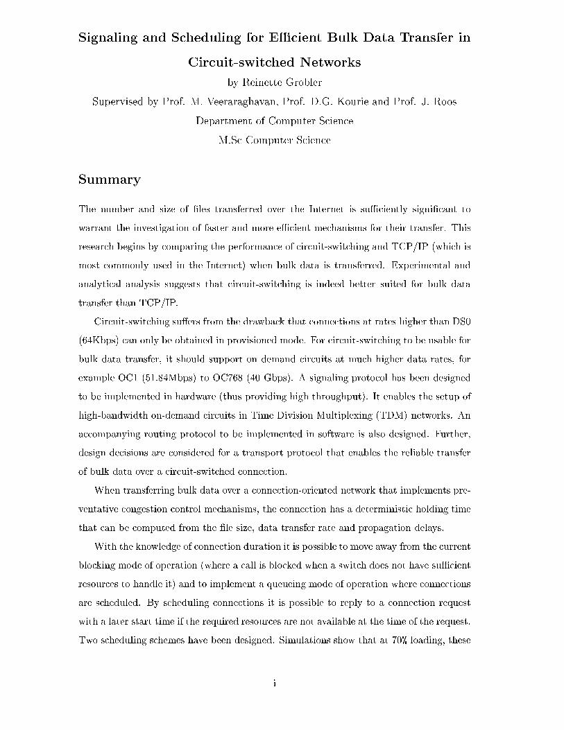
Summary
The number and size of �les transferred over the Internet is suÆciently signi�cant to
warrant the investigation of faster and more eÆcient mechanisms for their transfer. This
research begins by comparing the performance of circuit-switching and TCP/IP (which is
most commonly used in the Internet) when bulk data is transferred. Experimental and
analytical analysis suggests that circuit-switching is indeed better suited for bulk data
transfer than TCP/IP.
Circuit-switching su�ers from the drawback that connections at rates higher than DS0
(64Kbps) can only be obtained in provisioned mode. For circuit-switching to be usable for
bulk data transfer, it should support on demand circuits at much higher data rates, for
example OC1 (51.84Mbps) to OC768 (40 Gbps). A signaling protocol has been designed
to be implemented in hardware (thus providing high throughput). It enables the setup of
high-bandwidth on-demand circuits in Time Division Multiplexing (TDM) networks. An
accompanying routing protocol to be implemented in software is also designed. Further,
design decisions are considered for a transport protocol that enables the reliable transfer
of bulk data over a circuit-switched connection.
When transferring bulk data over a connection-oriented network that implements pre-
ventative congestion control mechanisms, the connection has a deterministic holding time
that can be computed from the �le size, data transfer rate and propagation delays.
With the knowledge of connection duration it is possible to move away from the current
blocking mode of operation (where a call is blocked when a switch does not have suÆcient
resources to handle it) and to implement a queueing mode of operation where connections
are scheduled. By scheduling connections it is possible to reply to a connection request
with a later start time if the required resources are not available at the time of the request.
Two scheduling schemes have been designed. Simulations show that at 70% loading, these
i

schemes o�er start time delays that are up to 85% smaller and channel utilization of up to
37% larger than a simple queueing mode of operation where call holding times are ignored
when connections are set up.
ii
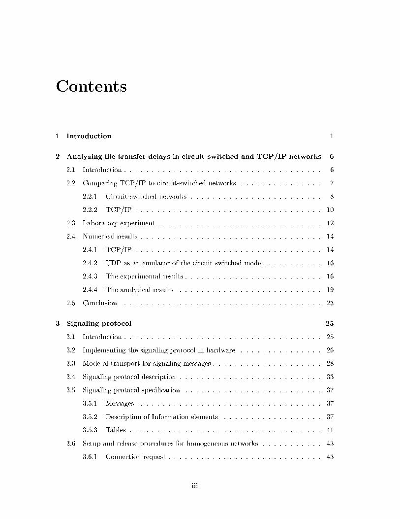
Contents
1 Introduction 1
2 Analyzing �le transfer delays in circuit-switched and TCP/IP networks 6
2.1 Introduction . . . . . . . . . . . . . . . . . . . . . . . . . . . . . . . . . . . . 6
2.2 Comparing TCP/IP to circuit-switched networks . . . . . . . . . . . . . . . 7
2.2.1 Circuit-switched networks . . . . . . . . . . . . . . . . . . . . . . . . 8
2.2.2 TCP/IP . . . . . . . . . . . . . . . . . . . . . . . . . . . . . . . . . . 10
2.3 Laboratory experiment . . . . . . . . . . . . . . . . . . . . . . . . . . . . . . 12
2.4 Numerical results . . . . . . . . . . . . . . . . . . . . . . . . . . . . . . . . . 14
2.4.1 TCP/IP . . . . . . . . . . . . . . . . . . . . . . . . . . . . . . . . . . 14
2.4.2 UDP as an emulator of the circuit switched mode . . . . . . . . . . . 16
2.4.3 The experimental results . . . . . . . . . . . . . . . . . . . . . . . . . 16
2.4.4 The analytical results . . . . . . . . . . . . . . . . . . . . . . . . . . 19
2.5 Conclusion . . . . . . . . . . . . . . . . . . . . . . . . . . . . . . . . . . . . 23
3 Signaling protocol 25
3.1 Introduction . . . . . . . . . . . . . . . . . . . . . . . . . . . . . . . . . . . . 25
3.2 Implementing the signaling protocol in hardware . . . . . . . . . . . . . . . 26
3.3 Mode of transport for signaling messages . . . . . . . . . . . . . . . . . . . . 28
3.4 Signaling protocol description . . . . . . . . . . . . . . . . . . . . . . . . . . 33
3.5 Signaling protocol speci�cation . . . . . . . . . . . . . . . . . . . . . . . . . 37
3.5.1 Messages . . . . . . . . . . . . . . . . . . . . . . . . . . . . . . . . . 37
3.5.2 Description of Information elements . . . . . . . . . . . . . . . . . . 37
3.5.3 Tables . . . . . . . . . . . . . . . . . . . . . . . . . . . . . . . . . . . 41
3.6 Setup and release procedures for homogeneous networks . . . . . . . . . . . 43
3.6.1 Connection request . . . . . . . . . . . . . . . . . . . . . . . . . . . . 43
iii
3.6.2 Connection establishment . . . . . . . . . . . . . . . . . . . . . . . . 44
3.6.3 Clearing a connection . . . . . . . . . . . . . . . . . . . . . . . . . . 44
3.7 Error conditions . . . . . . . . . . . . . . . . . . . . . . . . . . . . . . . . . 46
3.7.1 Cause values . . . . . . . . . . . . . . . . . . . . . . . . . . . . . . . 47
3.7.2 Timers . . . . . . . . . . . . . . . . . . . . . . . . . . . . . . . . . . . 47
3.7.3 Handling of error conditions . . . . . . . . . . . . . . . . . . . . . . . 49
3.8 Maximum bandwidth selection . . . . . . . . . . . . . . . . . . . . . . . . . 51
3.9 Improvements to signaling protocol . . . . . . . . . . . . . . . . . . . . . . . 52
3.9.1 Routing through heterogenous nodes . . . . . . . . . . . . . . . . . . 52
3.9.2 Transport of signaling messages . . . . . . . . . . . . . . . . . . . . . 55
3.10 Conclusion . . . . . . . . . . . . . . . . . . . . . . . . . . . . . . . . . . . . 56
4 Routing protocol 57
4.1 Introduction . . . . . . . . . . . . . . . . . . . . . . . . . . . . . . . . . . . . 57
4.2 Addressing . . . . . . . . . . . . . . . . . . . . . . . . . . . . . . . . . . . . 58
4.3 Design decisions . . . . . . . . . . . . . . . . . . . . . . . . . . . . . . . . . 61
4.4 Protocol description . . . . . . . . . . . . . . . . . . . . . . . . . . . . . . . 64
4.4.1 Routing database and directed graph . . . . . . . . . . . . . . . . . . 65
4.4.2 Constructing the shortest path tree . . . . . . . . . . . . . . . . . . . 69
4.4.3 Routing table . . . . . . . . . . . . . . . . . . . . . . . . . . . . . . . 71
4.5 Future work . . . . . . . . . . . . . . . . . . . . . . . . . . . . . . . . . . . . 73
5 Scheduling calls with known holding times 77
5.1 Introduction . . . . . . . . . . . . . . . . . . . . . . . . . . . . . . . . . . . . 77
5.2 Motivating applications . . . . . . . . . . . . . . . . . . . . . . . . . . . . . 79
5.3 Proposed algorithm . . . . . . . . . . . . . . . . . . . . . . . . . . . . . . . . 82
5.4 Extensions . . . . . . . . . . . . . . . . . . . . . . . . . . . . . . . . . . . . . 91
5.4.1 Request for start time included in connection request . . . . . . . . 91
5.4.2 More than one switch in the network . . . . . . . . . . . . . . . . . . 91
5.5 Connection setup schemes . . . . . . . . . . . . . . . . . . . . . . . . . . . . 93
5.5.1 The kTwait scheme . . . . . . . . . . . . . . . . . . . . . . . . . . . . 94
5.5.2 The kTwait � Tmax scheme . . . . . . . . . . . . . . . . . . . . . . . . 95
5.5.3 The F scheme . . . . . . . . . . . . . . . . . . . . . . . . . . . . . . 95
5.5.4 The timeslots scheme . . . . . . . . . . . . . . . . . . . . . . . . . . 101
iv
5.6 Simulation and results . . . . . . . . . . . . . . . . . . . . . . . . . . . . . . 104
5.6.1 Network model . . . . . . . . . . . . . . . . . . . . . . . . . . . . . . 104
5.6.2 Results . . . . . . . . . . . . . . . . . . . . . . . . . . . . . . . . . . 105
5.7 Further extensions and future work . . . . . . . . . . . . . . . . . . . . . . . 112
5.7.1 Switch programming delay . . . . . . . . . . . . . . . . . . . . . . . 112
5.7.2 Propagation delay computation . . . . . . . . . . . . . . . . . . . . . 113
5.7.3 Time . . . . . . . . . . . . . . . . . . . . . . . . . . . . . . . . . . . . 113
5.8 Summary and Conclusions . . . . . . . . . . . . . . . . . . . . . . . . . . . . 114
6 Further work: The transport layer 116
6.1 Introduction . . . . . . . . . . . . . . . . . . . . . . . . . . . . . . . . . . . . 116
6.2 Protocol requirements . . . . . . . . . . . . . . . . . . . . . . . . . . . . . . 117
6.3 Conclusion . . . . . . . . . . . . . . . . . . . . . . . . . . . . . . . . . . . . 120
7 Conclusion 121
Bibliography 123
v
List of Tables
1.1 Classi�cation of networking techniques . . . . . . . . . . . . . . . . . . . . . 1
1.2 Classi�cation of data transfers . . . . . . . . . . . . . . . . . . . . . . . . . . 2
2.1 Values used for �le sizes (f) in comparison of circuit-switching and TCP/IP 17
2.2 Parameters used in analytical comparison of circuit-switching and TCP . . 20
3.1 Description of parameters in SEND primitive [10] . . . . . . . . . . . . . . . 30
3.2 Description of parameters in RECV primitive [10] . . . . . . . . . . . . . . 31
3.3 Routing table . . . . . . . . . . . . . . . . . . . . . . . . . . . . . . . . . . . 34
3.4 Available bandwidth table including cost . . . . . . . . . . . . . . . . . . . . 35
3.5 Connectivity table . . . . . . . . . . . . . . . . . . . . . . . . . . . . . . . . 36
3.6 Switch mapping table . . . . . . . . . . . . . . . . . . . . . . . . . . . . . . 36
3.7 SETUP . . . . . . . . . . . . . . . . . . . . . . . . . . . . . . . . . . . . . . 37
3.8 SETUP SUCCESS . . . . . . . . . . . . . . . . . . . . . . . . . . . . . . . . 38
3.9 RELEASE . . . . . . . . . . . . . . . . . . . . . . . . . . . . . . . . . . . . . 38
3.10 RELEASE CONFIRM . . . . . . . . . . . . . . . . . . . . . . . . . . . . . . 38
3.11 Message types . . . . . . . . . . . . . . . . . . . . . . . . . . . . . . . . . . . 39
3.12 State table . . . . . . . . . . . . . . . . . . . . . . . . . . . . . . . . . . . . 42
3.13 Cause classes . . . . . . . . . . . . . . . . . . . . . . . . . . . . . . . . . . . 47
3.14 Cause values . . . . . . . . . . . . . . . . . . . . . . . . . . . . . . . . . . . 48
3.15 Routing table of switch 3 . . . . . . . . . . . . . . . . . . . . . . . . . . . . 54
4.1 ipS to ipR mapping table kept by SONET switch 1 . . . . . . . . . . . . . . 61
4.2 Available bandwidth table including cost . . . . . . . . . . . . . . . . . . . . 65
4.3 Routing database entry for node D from network depicted in Figure 4.2 . . 66
4.4 Routing update message . . . . . . . . . . . . . . . . . . . . . . . . . . . . . 68
4.5 Possible values for the cross connect rate of a switch . . . . . . . . . . . . . 69
vi
4.6 Directed graph . . . . . . . . . . . . . . . . . . . . . . . . . . . . . . . . . . 69
4.7 Predecessor list for SwitchB . . . . . . . . . . . . . . . . . . . . . . . . . . . 71
4.8 Routing table for node B . . . . . . . . . . . . . . . . . . . . . . . . . . . . 74
4.9 Routing table for Switch3 . . . . . . . . . . . . . . . . . . . . . . . . . . . . 75
5.1 Classi�cation of data transfers . . . . . . . . . . . . . . . . . . . . . . . . . . 80
5.2 Di�erent loads introduced by interference traÆc . . . . . . . . . . . . . . . . 106
5.3 Parameters used in simulation of connection setup schemes . . . . . . . . . 106
vii
List of Figures
1.1 Chapter layout . . . . . . . . . . . . . . . . . . . . . . . . . . . . . . . . . . 5
2.1 Emission delays, TCP/IP vs. circuit switching . . . . . . . . . . . . . . . . 8
2.2 Network con�guration used when transferring �le with TCP/IP . . . . . . . 13
2.3 Network con�guration used when transferring �le with UDP . . . . . . . . . 13
2.4 Establishing a TCP connection . . . . . . . . . . . . . . . . . . . . . . . . . 14
2.5 Closing a TCP connection . . . . . . . . . . . . . . . . . . . . . . . . . . . . 15
2.6 Comparison of transport protocols TCP and UDP . . . . . . . . . . . . . . 18
2.7 E�ect of propagation delay on TCP and circuit switching . . . . . . . . . . 21
2.8 E�ect of propagation delay on TCP and circuit switching, smaller �les . . . 22
2.9 E�ect of emission delay on TCP and circuit switching . . . . . . . . . . . . 22
2.10 E�ect of emission delay on TCP and circuit switching, smaller �les . . . . . 22
3.1 Ideal network in which signaling protocol will be used . . . . . . . . . . . . 28
3.2 Typical network in which signaling protocol will be used . . . . . . . . . . . 29
3.3 Primitives used between signaling process and IP module . . . . . . . . . . 29
3.4 Connectivity information . . . . . . . . . . . . . . . . . . . . . . . . . . . . 36
3.5 Signaling protocol state transition diagram . . . . . . . . . . . . . . . . . . 42
3.6 preceding/succeeding . . . . . . . . . . . . . . . . . . . . . . . . . . . . . . . 43
3.7 Successful setup of a connection . . . . . . . . . . . . . . . . . . . . . . . . . 44
3.8 Unsuccessful setup of a connection . . . . . . . . . . . . . . . . . . . . . . . 45
3.9 Normal connection release . . . . . . . . . . . . . . . . . . . . . . . . . . . . 45
3.10 Connection release by an intermediate node . . . . . . . . . . . . . . . . . . 46
3.11 Connection setup with minimum and maximum bandwidth requirements . . 52
3.12 Connection setup in heterogenous network . . . . . . . . . . . . . . . . . . . 53
3.13 Connection setup in large heterogenous network . . . . . . . . . . . . . . . . 54
viii
4.1 Routing network . . . . . . . . . . . . . . . . . . . . . . . . . . . . . . . . . 58
4.2 Example network con�guration for routing protocol . . . . . . . . . . . . . . 65
4.3 Shortest path tree constructed by node B . . . . . . . . . . . . . . . . . . . 71
4.4 Shortest path tree constructed by node B, with extra node . . . . . . . . . 72
4.5 Shortest path tree constructed by Switch3 . . . . . . . . . . . . . . . . . . . 74
5.1 A simple one switch network . . . . . . . . . . . . . . . . . . . . . . . . . . 83
5.2 Block diagram of a switch . . . . . . . . . . . . . . . . . . . . . . . . . . . . 84
5.3 Keys used in ow diagrams . . . . . . . . . . . . . . . . . . . . . . . . . . . 85
5.4 Flow chart for the message handling module in a one switch network . . . . 86
5.5 Flow chart for the message handling module in a one switch network, with
error handling . . . . . . . . . . . . . . . . . . . . . . . . . . . . . . . . . . . 87
5.6 Route lookup process included in the routing module . . . . . . . . . . . . . 88
5.7 Process to program the switch fabric in the switch programming module . . 88
5.8 Scheduling process included in the CAC module for a one switch network . 89
5.9 Process in the CAC module to undo the changes made by the scheduling
process . . . . . . . . . . . . . . . . . . . . . . . . . . . . . . . . . . . . . . 90
5.10 Scheduling process (allowing for a host to request a start time) included in
the CAC module for a one switch network . . . . . . . . . . . . . . . . . . . 92
5.11 Successful setup of a connection . . . . . . . . . . . . . . . . . . . . . . . . . 93
5.12 Connection setup at the ingress switch of a connection (F scheme) . . . . . 98
5.13 Process in the CAC module to update the changes made by the scheduling
process in the reverse direction . . . . . . . . . . . . . . . . . . . . . . . . . 99
5.14 Example of scheduled connection setup . . . . . . . . . . . . . . . . . . . . . 100
5.15 Available bandwidth of Switch1, interface i . . . . . . . . . . . . . . . . . . 101
5.16 Available bandwidth of Switch2, interface i . . . . . . . . . . . . . . . . . . 103
5.17 Network model . . . . . . . . . . . . . . . . . . . . . . . . . . . . . . . . . . 105
5.18 Percentage of calls blocked using di�erent connection setup schemes . . . . 107
5.19 Percentage of calls blocked using di�erent connection setup schemes, con-
stant mean interarrival times . . . . . . . . . . . . . . . . . . . . . . . . . . 108
5.20 Queueing delay experienced by connection requests for connections requir-
ing channel Switch1 -> Switch2 . . . . . . . . . . . . . . . . . . . . . . . . . 109
5.21 Start time delays for all connection setup schemes . . . . . . . . . . . . . . 109
ix
5.22 Start time delays for all connection setup schemes, constant mean interar-
rival times . . . . . . . . . . . . . . . . . . . . . . . . . . . . . . . . . . . . . 111
5.23 Utilization of channel Switch1->Switch2 . . . . . . . . . . . . . . . . . . . . 111
6.1 Transport layer in a connection oriented circuit switched network . . . . . . 118
x
Acronyms
ATM Asynchronous Transfer Mode
CAC Connection Admission Control
CL Connectionless
CO Connection oriented
ICMP Internet Control Message Protocol
IETF Internet Engineering Task Force
IP Internet Protocol
OSPF Open Shortest Path First
PDH Plesiochronous Digital Hierarchy
PSTN Public Switched Telephone Network
QoS Quality of Service
RIP Routing Information Protocol
SCTP Stream Control Transmission Protocol
SDH Synchronous Digital Hierarchy
SONET Synchronous Optical Network
TCP Transmission Control Protocol
TDM Time Division Multiplexing
TOS Type of Service
xi
TTL Time To Live
UDP User Datagram Protocol
WDM Wavelength Division Multiplexing
xii
Chapter 1
Introduction
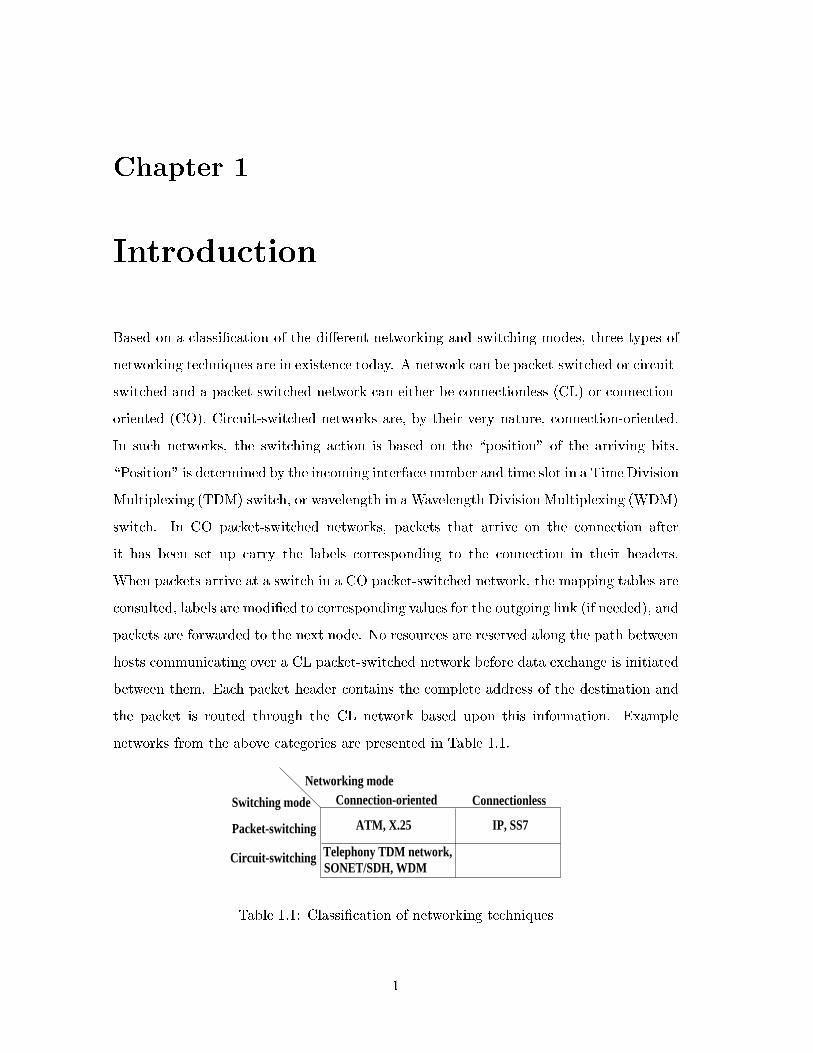
Based on a classi�cation of the di�erent networking and switching modes, three types of
networking techniques are in existence today. A network can be packet-switched or circuit-
switched and a packet-switched network can either be connectionless (CL) or connection-
oriented (CO). Circuit-switched networks are, by their very nature, connection-oriented.
In such networks, the switching action is based on the \position" of the arriving bits.
\Position" is determined by the incoming interface number and time slot in a Time Division
Multiplexing (TDM) switch, or wavelength in a Wavelength Division Multiplexing (WDM)
switch. In CO packet-switched networks, packets that arrive on the connection after
it has been set up carry the labels corresponding to the connection in their headers.
When packets arrive at a switch in a CO packet-switched network, the mapping tables are
consulted, labels are modi�ed to corresponding values for the outgoing link (if needed), and
packets are forwarded to the next node. No resources are reserved along the path between
hosts communicating over a CL packet-switched network before data exchange is initiated
between them. Each packet header contains the complete address of the destination and
the packet is routed through the CL network based upon this information. Example
networks from the above categories are presented in Table 1.1.
Networking mode
Switching mode Connection-oriented Connectionless
Packet-switching
Circuit-switching Telephony TDM network,
ATM, X.25 IP, SS7
SONET/SDH, WDM
Table 1.1: Classi�cation of networking techniques
1
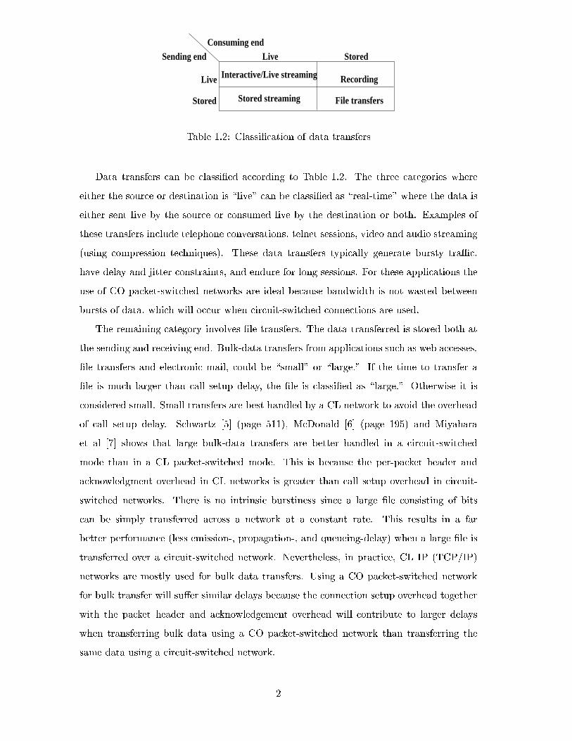
Recording
Sending endConsuming end
Live Stored
Stored
Live
File transfersStored streaming
Interactive/Live streaming
Table 1.2: Classi�cation of data transfers
Data transfers can be classi�ed according to Table 1.2. The three categories where
either the source or destination is \live" can be classi�ed as \real-time" where the data is
either sent live by the source or consumed live by the destination or both. Examples of
these transfers include telephone conversations, telnet sessions, video and audio streaming
(using compression techniques). These data transfers typically generate bursty traÆc,
have delay and jitter constraints, and endure for long sessions. For these applications the
use of CO packet-switched networks are ideal because bandwidth is not wasted between
bursts of data, which will occur when circuit-switched connections are used.
The remaining category involves �le transfers. The data transferred is stored both at
the sending and receiving end. Bulk-data transfers from applications such as web accesses,
�le transfers and electronic mail, could be \small" or \large." If the time to transfer a
�le is much larger than call setup delay, the �le is classi�ed as \large." Otherwise it is
considered small. Small transfers are best handled by a CL network to avoid the overhead
of call setup delay. Schwartz [5] (page 511), McDonald [6] (page 195) and Miyahara
et al [7] shows that large bulk-data transfers are better handled in a circuit-switched
mode than in a CL packet-switched mode. This is because the per-packet header and
acknowledgment overhead in CL networks is greater than call setup overhead in circuit-
switched networks. There is no intrinsic burstiness since a large �le consisting of bits
can be simply transferred across a network at a constant rate. This results in a far
better performance (less emission-, propagation-, and queueing-delay) when a large �le is
transferred over a circuit-switched network. Nevertheless, in practice, CL IP (TCP/IP)
networks are mostly used for bulk data transfers. Using a CO packet-switched network
for bulk transfer will su�er similar delays because the connection setup overhead together
with the packet header and acknowledgement overhead will contribute to larger delays
when transferring bulk data using a CO packet-switched network than transferring the
same data using a circuit-switched network.
2
Two types of circuit-switched networks are in use today. Time Division Multiplex-
ing (TDM) is the simplest circuit-switched network where the switching action is per-
formed based on the incoming interface number and time slot. Wavelength Division
Multiplexing (WDM) switches base their switching decision on the incoming interface
number and wavelength of the arriving bits. Currently, in both types of circuit-switched
networks, on demand (referred to as \switched" mode of operation as opposed to \pro-
visioned" mode) circuits can only be obtained at the DS0 (64 Kbps) rate, and the only
application that uses switched circuits is telephony. All higher rate circuits are used in
provisioned (hardwired) mode where circuits are established a priori across the network
and are changed infrequently.
To support large bulk-data transfers from applications such as web accesses, �le trans-
fers and electronic mail, a network will have to accommodate high-bandwidth (higher than
DS0) on-demand circuits between any two nodes of the network. Considering that the high-
speed circuit-switched network, Synchronous Optical Networks/Synchronous Digital Hier-
archy (SONET/SDH), is able to provide circuits with bandwidth from OC1(51.84Mbps) up
to OC768 (40 Gbps), there is a need for a mechanism to set up on-demand circuits for the
bene�t of increasing performance experienced by �le transfer applications. Transferring a
large �le over even the least-bandwidth SONET circuit (51.84Mbps) will improve delays
considerably when compared to the commonly used TCP protocol over the connectionless
IP network.
In a CO network, connection setup and release procedures, along with the associated
message exchanges, constitute the signaling protocol. Moving away from the telephony ap-
plication, a new signaling protocol is required for the circuit-switched networks to support
these high-bandwidth on-demand circuits.
Signaling protocols are typically implemented in software. This is due to the com-
plexity of signaling messages, and the amount of state information that needs to be kept
by all switches participating in connection setup. The fact that signaling protocols are
implemented in software points to a shortcoming in circuit-switched networks. Switch
fabrics are continually improved to handle data at faster speeds, but that is only after a
connection has been set up. Implementing signaling protocols in hardware could signi�-
cantly increase switches' call handling capabilities. The expected increase in call handling
capacities of switches will dramatically a�ect the role circuit-switched networks play in
future data transfer applications. This dissertation presents a novel signaling protocol
3
intended for hardware implementation.
In support of the new signaling protocol, an accompanying routing protocol (to be
implemented in software) is designed. The routing protocol provides enough information
to the signaling protocol for eÆcient connection setup along the shortest path between the
source and destination.
An experimental analysis of circuit-switching, done as part of this research, suggest-
s that an improvement in network utilization can be expected based on an important
characteristic of �le transfer applications. The characteristic of interest is that if a �le is
transferred over a circuit-switched network (that implements preventative congestion con-
trol as opposed to reactive congestion control in TCP/IP networks), the holding time of
the required connection can be deduced from the �le size. In connection-oriented networks,
connections are admitted without knowledge of the call holding time. If resources are not
available, the connection request is simply denied and connection release procedures are
initiated by the signaling protocol. This dissertation explores the option of queueing calls
in connection-oriented networks instead of blocking them when network resources are una-
vailable. A simple call queueing algorithm is to hold up call setup messages at each switch
along an end-to-end path until resources become available. This approach is used in the
analysis described in Miyahara et al's paper [7]. This scheme su�ers from poor network
utilization and long call queueing delays. However, if calls have known holding times, it
is possible to design call scheduling algorithms that result in reduced call queueing delays
and improved network utilization. Algorithms for such call scheduling are proposed and
the quantitative bene�ts of algorithms that exploit knowledge of call holding times are
demonstrated.
The author was a member of the CATT (Center for Advanced Technology in Telecom-
munications) research group at Polytechnic University, Brooklyn, New York, and is re-
sponsible for the design of the signaling protocol, the supporting routing protocol as well
as the design and simulation of the scheduling algorithms. The scheduling algorithms
presented in Chapter 5 has a US patent pending, reference number IDS 122874. Other
CATT team members are currently exploring hardware implementation of the signaling
protocol presented in Chapter 3, and busy designing a transport protocol to be used over
a circuit for bulk data transfers.
Chapter 2 explores the performance gains that can be expected when a circuit-switched
network is used for bulk data transfers. To provide a better understanding of the per-
4
Chapter 2Analyzing file transfer delays in
circuit-switched and TCP/IP networks.
Chapter 6Further work:
Transport layer
Chapter 3
Signaling protocol
Chapter 5Scheduling calls with known holding times
Chapter 4
Routing protocol
Figure 1.1: Chapter layout
formance gains an experiment was designed to compare data transfer characteristics of
TCP/IP and circuit-switched networks. Chapter 3 introduces the signaling protocol for
use in a connection-oriented circuit-switched network, in this case a TDM network, and
Chapter 4 provides a solution for the supporting routing protocol. Chapter 5 describes
some solutions that can be used to improve connection admission by making use of the
holding time of the connection to schedule the start of a connection for a later time if the
requested resources are not available at the time of connection request. Chapter 6 notes
future work, which is the transport protocol that is required to enable the reliable transfer
of data over a circuit-switched network.
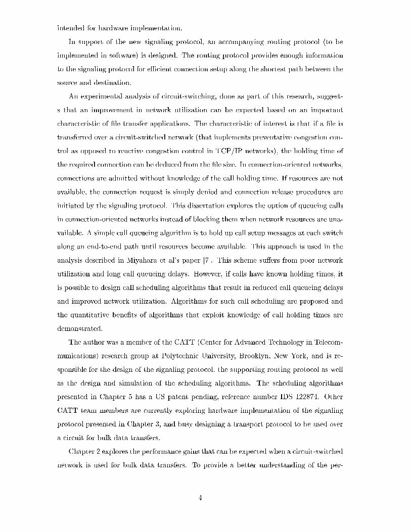
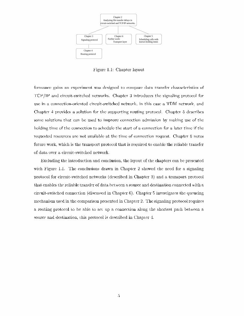
Excluding the introduction and conclusion, the layout of the chapters can be presented
with Figure 1.1. The conclusions drawn in Chapter 2 showed the need for a signaling
protocol for circuit-switched networks (described in Chapter 3) and a transport protocol
that enables the reliable transfer of data between a source and destination connected with a
circuit-switched connection (discussed in Chapter 6). Chapter 5 investigates the queueing
mechanism used in the comparison presented in Chapter 2. The signaling protocol requires
a routing protocol to be able to set up a connection along the shortest path between a
source and destination, this protocol is described in Chapter 4.
5
Chapter 2
Analyzing �le transfer delays in
circuit-switched and TCP/IP
networks
2.1 Introduction
Chapter 2Analyzing file transfer delays in
circuit-switched and TCP/IP networks.
Chapter 6Further work:
Transport layer
Chapter 3
Signaling protocol
Chapter 5Scheduling calls with known holding times
Chapter 4
Routing protocol
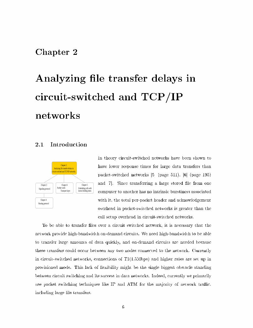
In theory circuit-switched networks have been shown to
have lower response times for large data transfers than
packet-switched networks [5] (page 511), [6] (page 195)
and [7]. Since transferring a large stored �le from one
computer to another has no intrinsic burstiness associated
with it, the total per-packet header and acknowledgement
overhead in packet-switched networks is greater than the
call setup overhead in circuit-switched networks.
To be able to transfer �les over a circuit switched network, it is necessary that the
network provide high-bandwidth on-demand circuits. We need high-bandwidth to be able
to transfer large amounts of data quickly, and on-demand circuits are needed because
these transfers could occur between any two nodes connected to the network. Currently
in circuit-switched networks, connections of T1(1.5Mbps) and higher rates are set up in
provisioned mode. This lack of exibility might be the single biggest obstacle standing
between circuit switching and its success in data networks. Indeed, currently we primarily
use packet switching techniques like IP and ATM for the majority of network traÆc,
including large �le transfers.
6
This chapter attempts to associate real world numbers with the comparisons in [5] and
[7], starting by moving from general packet switching techniques to TCP/IP. TCP/IP is
currently the packet switching technique of choice when large �les are transferred over the
Internet. Comparing TCP/IP to circuit-switching under laboratory conditions is intended
to help us understand the performance we currently experience and to anticipate the
performance we should expect if we decided to make use of circuit-switching for all large
�le transfers. Note that in this discussion, a large �le is considered to be a �le for which
the total transfer time of the per-packet overhead and the acknowledgement overhead is
greater than the call setup overhead in circuit-switched networks.
Due to the unavailability of a circuit-switched network that provides high-bandwidth
on-demand circuits, we used UDP together with a simple network con�guration to simulate
circuit-switching. Section 2.2 describes the equations we designed for the comparison,
Section 2.3 introduces the reader to the testing environment and the goals of the speci�c
tests, Section 2.4 describes the results of the tests and Section 2.5 is the conclusion.
2.2 Comparing TCP/IP to circuit-switched networks
When transferring a �le, delay can be categorized as follows:
� propagation delay
� emission delay
� queueing delay
� processing delay
In a large network with long round trip times, propagation delay will have a signi�cant
in uence on the transfer time when TCP/IP is used. This is because of the presence of
ACK messages. Before the maximum window size is used by the client, the propagation
delay incurred by the ACKs will be signi�cant.
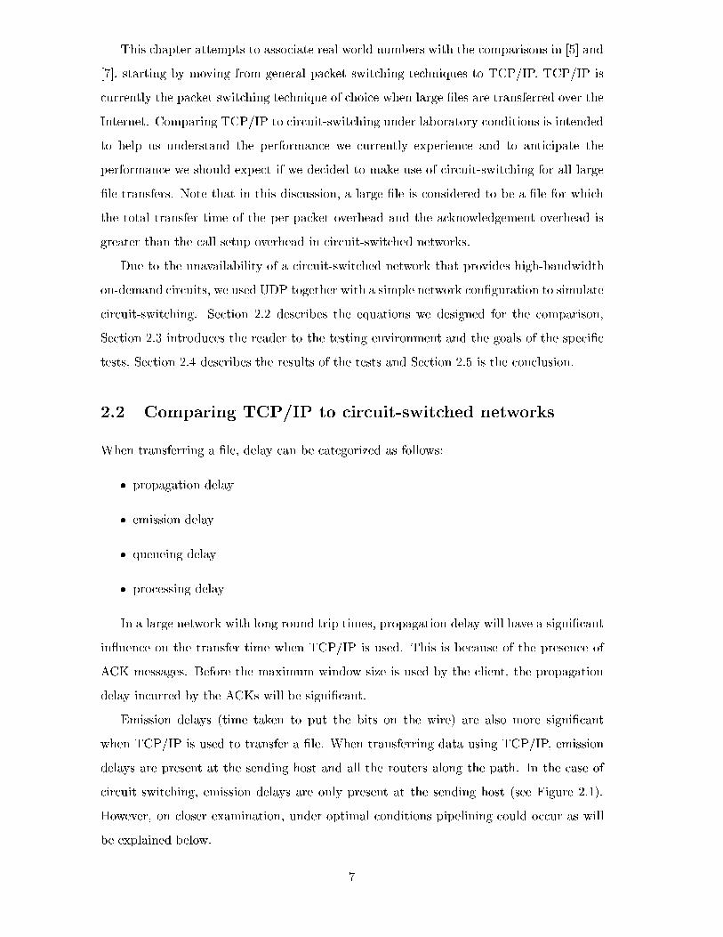
Emission delays (time taken to put the bits on the wire) are also more signi�cant
when TCP/IP is used to transfer a �le. When transferring data using TCP/IP, emission
delays are present at the sending host and all the routers along the path. In the case of
circuit switching, emission delays are only present at the sending host (see Figure 2.1).
However, on closer examination, under optimal conditions pipelining could occur as will
be explained below.
7

X X XEH EH
R R REH EH
Emission delay
Figure 2.1: Emission delays, TCP/IP vs. circuit switching
The queueing and processing delays (experienced at routers when incoming packets
are queued and processed) are also only present when sending the �le via TCP/IP, not
when the �le is sent using circuit switching. Once a circuit has been set up between the
source and destination hosts, the data is switched by each intermediate switch without it
experiencing queueing and processing delays.
To better understand the total time taken to transfer a large �le using TCP/IP vs. a
fast circuit, we �rst propose mathematical models of the time delays in each respective
case. Sections 2.2.1 and 2.2.2 present the mathematical models for circuit-switching and
TCP/IP respectively.
2.2.1 Circuit-switched networks
Tckt = Tsetup + kTwait + Ttransfer (f) (2.1)
Tsetup = kTproc + Tr:t:prop + 2 (k + 1)
�s+ ovhd
rate
�(2.2)
Ttransfer (f) =Tr:t:prop
2+
f + ovhd
rate(2.3)
In the above equations, all the times (T ) are the average times, s is the length of the
signaling message, f is the �le size, Tr:t:prop denotes the round-trip propagation delay and k
indicates the number of switches. Twait is the time to wait for the requested resources to be
freed (assuming a queueing mode of operation is used, as opposed to a call blocking mode).
Tproc indicates the total processing delay that includes route determination, Connection
8
Admission Control (CAC) and switch programming, incurred at a switch to set up a
connection.
The overhead (ovhd) included in Equation (2.2) and (2.3) is the overhead introduced
by the data link layer (for example SONET). If the transport layer implements a FEC
(Forward Error Correction) scheme (supplemented with NAKs), the overhead will include
more than just the headers added by the lower protocol layers.
Equation (2.1) is the total time needed to transfer a �le using a circuit. Together with
the processing delay (Tproc) experienced by a connection request captured in the term
Tsetup, the signaling message requesting the connection is also placed in a queue at each
switch to wait for the required resources to be released. Only when the connection request
reaches the head of the queue, and its requested resources are available, will the request
be passed on to the next switch. Hence the term kTwait.
Equation (2.2) includes the processing delay at switches, propagation delay, and emis-
sion delay (which is the length of signaling messages divided by the data rate used for
signaling). It is assumed that a circuit is set up using two messages: typically a SETUP is
sent in the forward direction from the source to the destination; if all the switches along
the path and the destination are able to handle the connection, a SETUP SUCCESS mes-
sage is sent in the reverse direction from the destination to the source. After processing
each of these messages at each switch, a signaling message has to be re-introduced to the
circuit-switched network. This has the consequence that the emission delay is computed
for each switch (each switch places the signaling message \on the wire" to the next switch)
as well as for the end hosts responsible for sending the message. Thus signaling messages
have to be placed on (k + 1) links during connection setup in both the forward and reverse
directions. Hence the term 2 (k + 1).
During �le transfer (see Equation (2.3)), there is no queueing delay since these are
circuit switches and only emission and propagation delays are incurred. The emission delay
is also only incurred at the sending host. This is because after a circuit has been set up, the
host initially places the bits on the wire after which it is switched by each intermediate
node without experiencing queueing, processing or emission delays. It is assumed that
the �le transfer is initiated from the sending host, and the connection is closed by the
sending host after the error free �le transmission has completed. The consequence of this
assumption is that the �le transfer does not include a round trip delay, but only delay for
transfer in one direction.
9
Time to release a circuit incurs the same three delays as to set up a circuit. When
the sending host closes the connection, it sends a message with its request to its ingress
switch. After receiving a reply to this message, the connection is considered closed by the
sending host. The total time for release is not directly included in the �le transfer delay
model given here, but the e�ect of release messages on queueing delays of setup messages
should be considered.
2.2.2 TCP/IP
The following equations are obtained if it is assumed that there is no loss of packets and
hence that the congestion window grows steadily with the sender sending 1 segment, and
then 2, and then 4 and so on, until the whole �le is sent. One ACK is assumed for
each \group" of segments. It is also assumed that ssthresh is not reached and that TCP
continues operating in slow start. In these equations k indicates the number of routers, m
indicates the maximum segment size (in bytes) in TCP/IP and e-e indicates end-to-end.
TTCP = Te�esetup + Ttransfer (f) + Te�eclose (2.4)
Equation (2.4) is the total time needed to transfer a �le using TCP.
Te�esetup = Te�eproc + Tr:t:prop: + 3 (k + 1)
�s+ ovhd
rate
�(2.5)
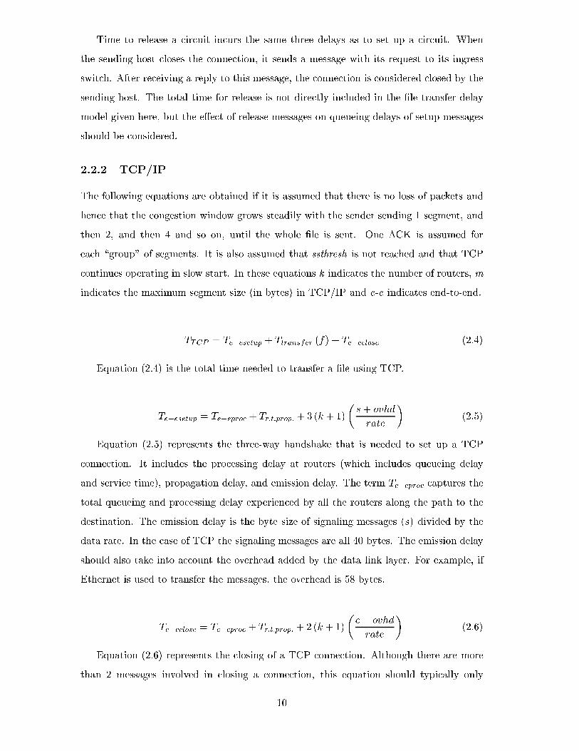
Equation (2.5) represents the three-way handshake that is needed to set up a TCP
connection. It includes the processing delay at routers (which includes queueing delay
and service time), propagation delay, and emission delay. The term Te�eproc captures the
total queueing and processing delay experienced by all the routers along the path to the
destination. The emission delay is the byte size of signaling messages (s) divided by the
data rate. In the case of TCP the signaling messages are all 40 bytes. The emission delay
should also take into account the overhead added by the data link layer. For example, if
Ethernet is used to transfer the messages, the overhead is 58 bytes.
Te�eclose = Te�eproc + Tr:t:prop: + 2 (k + 1)
�c+ ovhd
rate
�(2.6)
Equation (2.6) represents the closing of a TCP connection. Although there are more
than 2 messages involved in closing a connection, this equation should typically only
10
correspond to the last 2 messages. This is because only the last two messages do not
contain data or acknowledgements corresponding to received data. The time delays caused
by other segments responsible for closing the connection are included in the �le transfer
time computation. The time taken to close a TCP connection incurs the same three delay
components as were discussed in setting up a connection.
Ttransfer (f) = NTr:t:prop + Temission + Ttotal�svc + Tack (2.7)
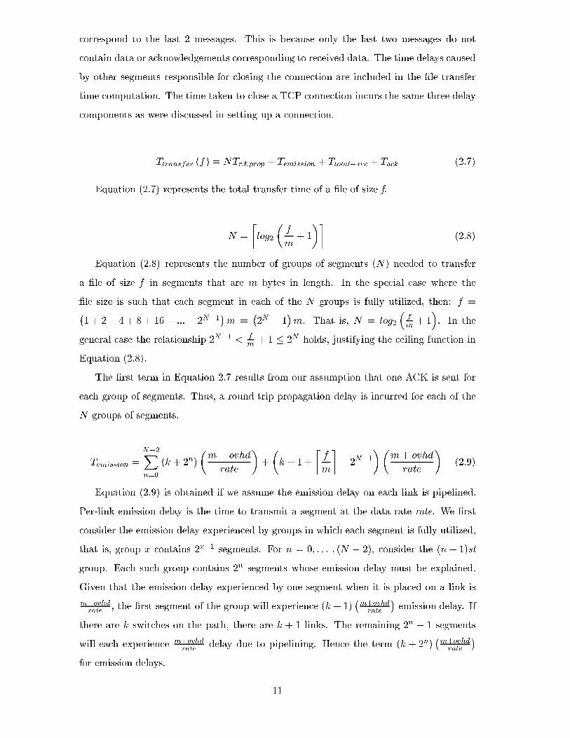
Equation (2.7) represents the total transfer time of a �le of size f.
N =
�log2
�f
m+ 1
��(2.8)
Equation (2.8) represents the number of groups of segments (N) needed to transfer
a �le of size f in segments that are m bytes in length. In the special case where the
�le size is such that each segment in each of the N groups is fully utilized, then: f =�1 + 2 + 4 + 8 + 16 + :::+ 2N�1
�m =
�2N � 1
�m. That is, N = log2
�fm+ 1
�. In the
general case the relationship 2N�1 < fm+ 1 � 2N holds, justifying the ceiling function in
Equation (2.8).
The �rst term in Equation 2.7 results from our assumption that one ACK is sent for
each group of segments. Thus, a round trip propagation delay is incurred for each of the
N groups of segments.
Temission =
N�2Xn=0
(k + 2n)
�m+ ovhd
rate
�+
�k + 1 +
�f
m
�� 2N�1
��m+ ovhd
rate
�(2.9)
Equation (2.9) is obtained if we assume the emission delay on each link is pipelined.
Per-link emission delay is the time to transmit a segment at the data rate rate. We �rst
consider the emission delay experienced by groups in which each segment is fully utilized,
that is, group x contains 2x�1 segments. For n = 0; : : : ; (N � 2), consider the (n+ 1)st
group. Each such group contains 2n segments whose emission delay must be explained.
Given that the emission delay experienced by one segment when it is placed on a link is
m+ovhdrate
, the �rst segment of the group will experience (k + 1)�m+ovhdrate
�emission delay. If
there are k switches on the path, there are k + 1 links. The remaining 2n � 1 segments
will each experience m+ovhdrate
delay due to pipelining. Hence the term (k + 2n)�m+ovhdrate
�for emission delays.
11
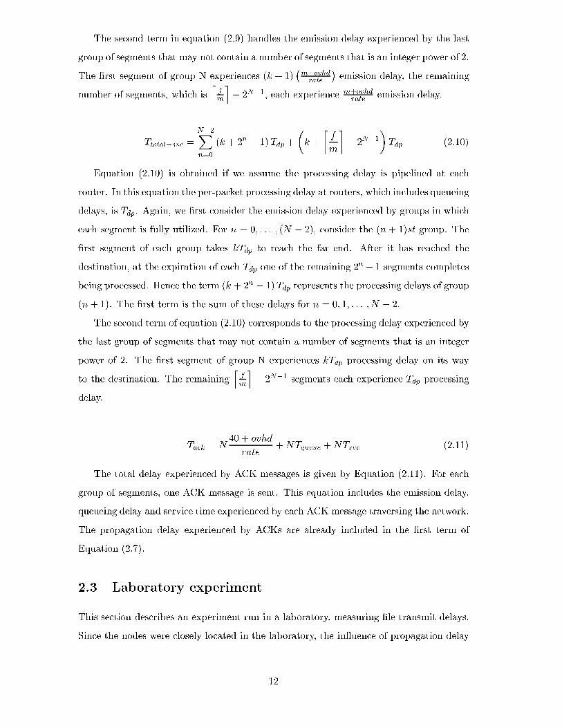
The second term in equation (2.9) handles the emission delay experienced by the last
group of segments that may not contain a number of segments that is an integer power of 2.
The �rst segment of group N experiences (k + 1)�m+ovhdrate
�emission delay, the remaining
number of segments, which islfm
m� 2N�1, each experience m+ovhd
rateemission delay.
Ttotal�svc =
N�2Xn=0
(k + 2n � 1) Tdp +
�k +
�f
m
�� 2N�1
�Tdp (2.10)
Equation (2.10) is obtained if we assume the processing delay is pipelined at each
router. In this equation the per-packet processing delay at routers, which includes queueing
delays, is Tdp. Again, we �rst consider the emission delay experienced by groups in which
each segment is fully utilized. For n = 0; : : : ; (N � 2), consider the (n+ 1)st group. The
�rst segment of each group takes kTdp to reach the far end. After it has reached the
destination, at the expiration of each Tdp one of the remaining 2n � 1 segments completes
being processed. Hence the term (k + 2n � 1) Tdp represents the processing delays of group
(n+ 1). The �rst term is the sum of these delays for n = 0; 1; : : : ; N � 2.
The second term of equation (2.10) corresponds to the processing delay experienced by
the last group of segments that may not contain a number of segments that is an integer
power of 2. The �rst segment of group N experiences kTdp processing delay on its way
to the destination. The remaininglfm
m� 2N�1 segments each experience Tdp processing
delay.
Tack = N40 + ovhd
rate+NTqueue +NTsvc (2.11)
The total delay experienced by ACK messages is given by Equation (2.11). For each
group of segments, one ACK message is sent. This equation includes the emission delay,
queueing delay and service time experienced by each ACK message traversing the network.
The propagation delay experienced by ACKs are already included in the �rst term of
Equation (2.7).
2.3 Laboratory experiment
This section describes an experiment run in a laboratory, measuring �le transmit delays.
Since the nodes were closely located in the laboratory, the in uence of propagation delay
12
on the overall transmission time was negligible. Instead, the emission and queueing delays
were kept in mind when the network con�guration was made.
Tests were conducted with a Sun SPARC4 workstation, an Intel PIII500 workstation
and two Cisco 2500 routers, all connected with 10 Mbps Ethernet.
In all experiments the term \server" refers to the machine that sends a large �le to
the \client" that requested the �le.
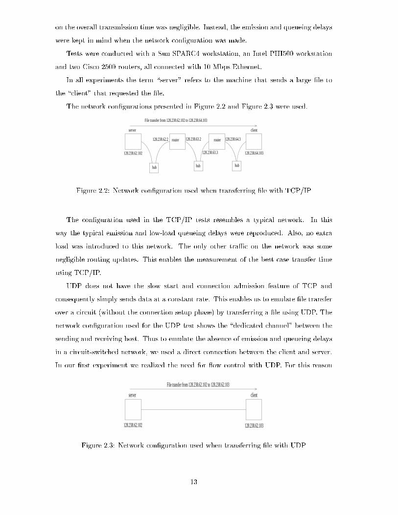
The network con�gurations presented in Figure 2.2 and Figure 2.3 were used.
hub
router
hub hub
server
File transfer from 128.238.62.102 to 128.238.64.103
128.238.62.102
128.238.62.2 router
128.238.63.3
128.238.64.3
128.238.64.103
client
128.238.63.2
Figure 2.2: Network con�guration used when transferring �le with TCP/IP
The con�guration used in the TCP/IP tests resembles a typical network. In this
way the typical emission and low-load queueing delays were reproduced. Also, no extra
load was introduced to this network. The only other traÆc on the network was some
negligible routing updates. This enables the measurement of the best case transfer time
using TCP/IP.
UDP does not have the slow start and connection admission feature of TCP and
consequently simply sends data at a constant rate. This enables us to emulate �le transfer
over a circuit (without the connection setup phase) by transferring a �le using UDP. The
network con�guration used for the UDP test shows the \dedicated channel" between the
sending and receiving host. Thus to emulate the absence of emission and queueing delays
in a circuit-switched network, we used a direct connection between the client and server.
In our �rst experiment we realized the need for ow control with UDP. For this reason
server client
128.238.62.102
File transfer from 128.238.62.102 to 128.238.62.103
128.238.62.103
Figure 2.3: Network con�guration used when transferring �le with UDP
13
13:44:38.354435 128.238.62.102.32788 > 128.238.64.103.6234: S
1569190891:1569190891(0) win 8760 <mss 1460> (DF)
13:44:38.354482 128.238.64.103.6234 > 128.238.62.102.32788: S
169214293:169214293(0) ack 1569190892 win 32120
<mss 1460> (DF)
13:44:38.356011 128.238.62.102.32788 > 128.238.64.103.6234: .
ack 1 win 8760 (DF)
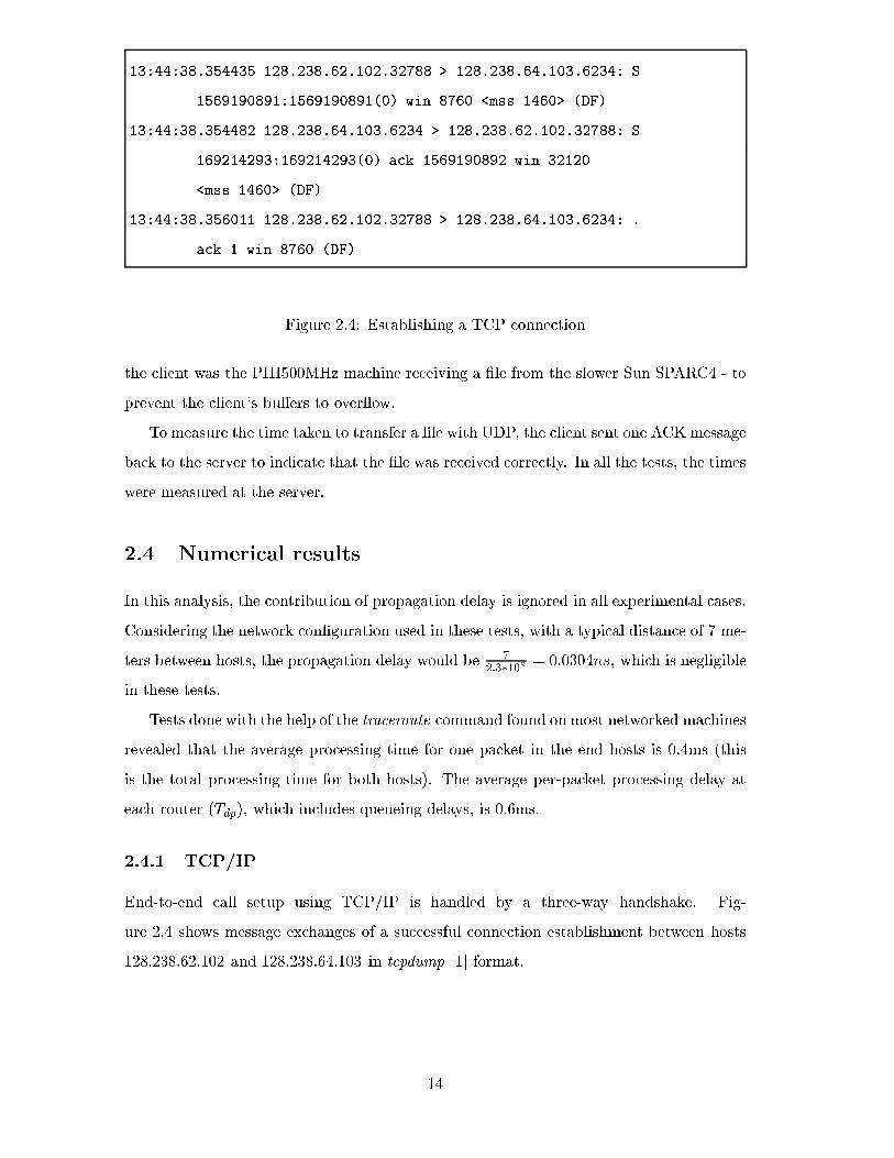
Figure 2.4: Establishing a TCP connection
the client was the PIII500MHz machine receiving a �le from the slower Sun SPARC4 - to
prevent the client's bu�ers to over ow.
To measure the time taken to transfer a �le with UDP, the client sent one ACK message
back to the server to indicate that the �le was received correctly. In all the tests, the times
were measured at the server.
2.4 Numerical results
In this analysis, the contribution of propagation delay is ignored in all experimental cases.
Considering the network con�guration used in these tests, with a typical distance of 7 me-
ters between hosts, the propagation delay would be 7
2:3�108= 0:0304ns, which is negligible
in these tests.
Tests done with the help of the traceroute command found on most networked machines
revealed that the average processing time for one packet in the end hosts is 0.4ms (this
is the total processing time for both hosts). The average per-packet processing delay at
each router (Tdp), which includes queueing delays, is 0.6ms.
2.4.1 TCP/IP
End-to-end call setup using TCP/IP is handled by a three-way handshake. Fig-
ure 2.4 shows message exchanges of a successful connection establishment between hosts
128.238.62.102 and 128.238.64.103 in tcpdump [1] format.
14
13:44:51.427515 128.238.62.102.32788 > 128.238.64.103.6234: F
9730049:9731181(1132) ack 1 win 8760 (DF)
13:44:51.427536 128.238.64.103.6234 > 128.238.62.102.32788: .
ack 9731182 win 30987 (DF)
13:44:51.427775 128.238.64.103.6234 > 128.238.62.102.32788: F
1:1(0) ack 9731182 win 32120 (DF)
13:44:51.429244 128.238.62.102.32788 > 128.238.64.103.6234: .
ack 2 win 8760 (DF)
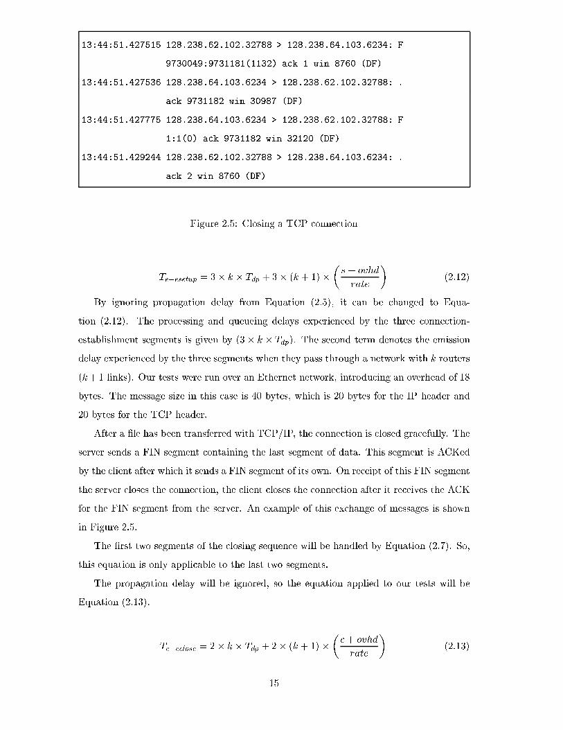
Figure 2.5: Closing a TCP connection
Te�esetup = 3� k � Tdp + 3� (k + 1)�
�s+ ovhd
rate
�(2.12)
By ignoring propagation delay from Equation (2.5), it can be changed to Equa-
tion (2.12). The processing and queueing delays experienced by the three connection-
establishment segments is given by (3� k � Tdp). The second term denotes the emission
delay experienced by the three segments when they pass through a network with k routers
(k+1 links). Our tests were run over an Ethernet network, introducing an overhead of 18
bytes. The message size in this case is 40 bytes, which is 20 bytes for the IP header and
20 bytes for the TCP header.
After a �le has been transferred with TCP/IP, the connection is closed gracefully. The
server sends a FIN segment containing the last segment of data. This segment is ACKed
by the client after which it sends a FIN segment of its own. On receipt of this FIN segment
the server closes the connection, the client closes the connection after it receives the ACK
for the FIN segment from the server. An example of this exchange of messages is shown
in Figure 2.5.
The �rst two segments of the closing sequence will be handled by Equation (2.7). So,
this equation is only applicable to the last two segments.
The propagation delay will be ignored, so the equation applied to our tests will be
Equation (2.13).
Te�eclose = 2� k � Tdp + 2� (k + 1)�
�c+ ovhd
rate
�(2.13)
15
In Equation (2.13) the processing and queueing delay experienced by the last two
segments is given by (2� k � Tdp), and the second term denotes the emission delay expe-
rienced by the two segments when they pass through a network with k routers.
The TCP/IP implementation used for the tests implemented the ACK strategy of
\ACK every other segment." This is di�erent from our assumption used in Section 2.2,
which stated that an ACK is generated for every group of segments. In none of our tests
was delay introduced at the server due to a late acknowledgement. For this reason, the
term Tack shall be ignored in our analysis. This change to Equation (2.7), together with
the removal of the term containing propagation delay produces Equation (2.14) in which
the emission and processing delays are represented. Equations (2.9) and (2.10) respectively
model these delays.
Ttransfer (f) = Ttotal�svc + Temission (2.14)
2.4.2 UDP as an emulator of the circuit switched mode
There is no connection setup phase in UDP, so the total transfer time can be given by
Equation (2.15) which is similar to Equation (2.3) (the equation for the time taken to
transfer a �le of size f over a circuit switched network). The reason why the propagation
delay is not halved to indicate the transfer time is because, in the UDP case, an ACK
message is sent from the client to the server to indicate successful receipt of the data.
The propagation delay will still be ignored due to its insigni�cant size, so the equations
can be thought of as exactly the same in the laboratory environment. The second term
of Equation (2.16) shows the ACK that is sent from the client to the server to indicate
successful receipt of the �le.
Ttransfer = Tr:t:prop +f + ovhd
rate(2.15)
f = filesize+ 512 (2.16)
2.4.3 The experimental results
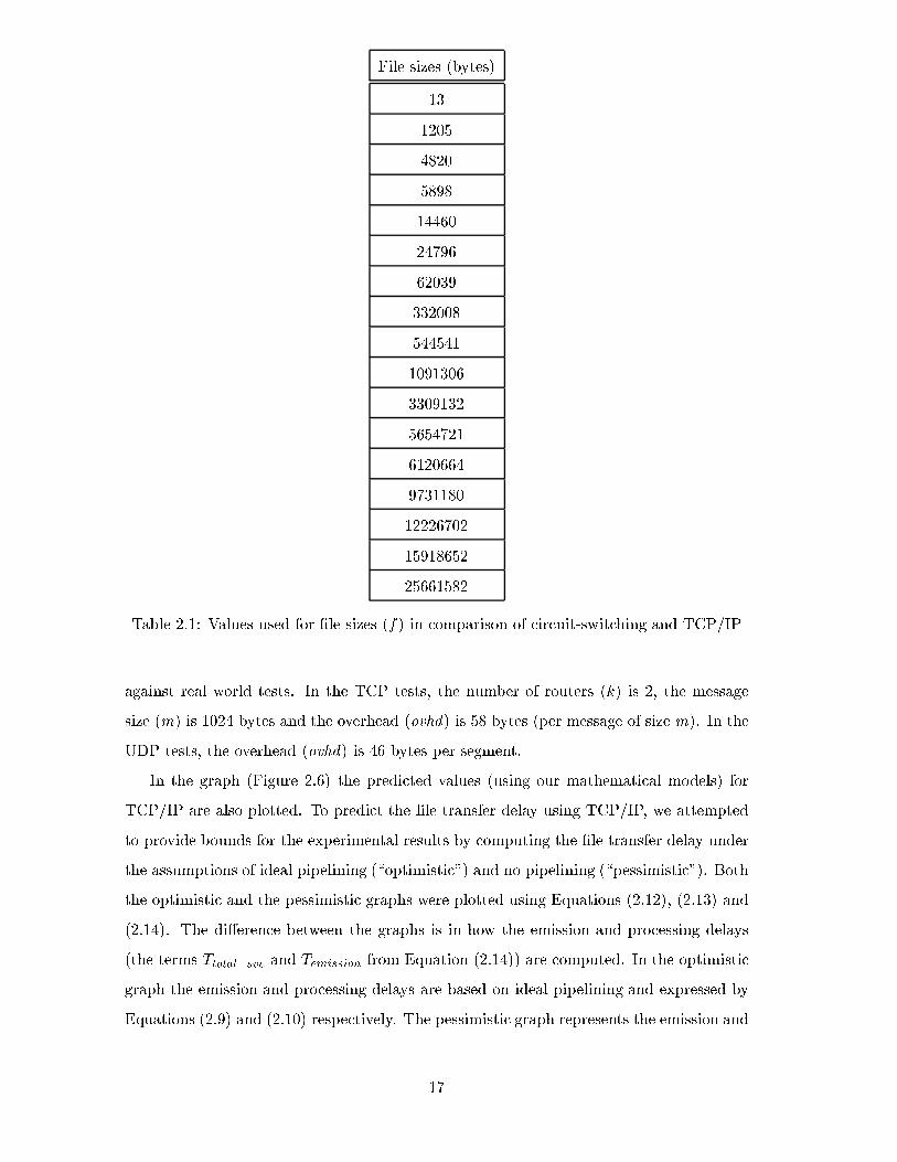
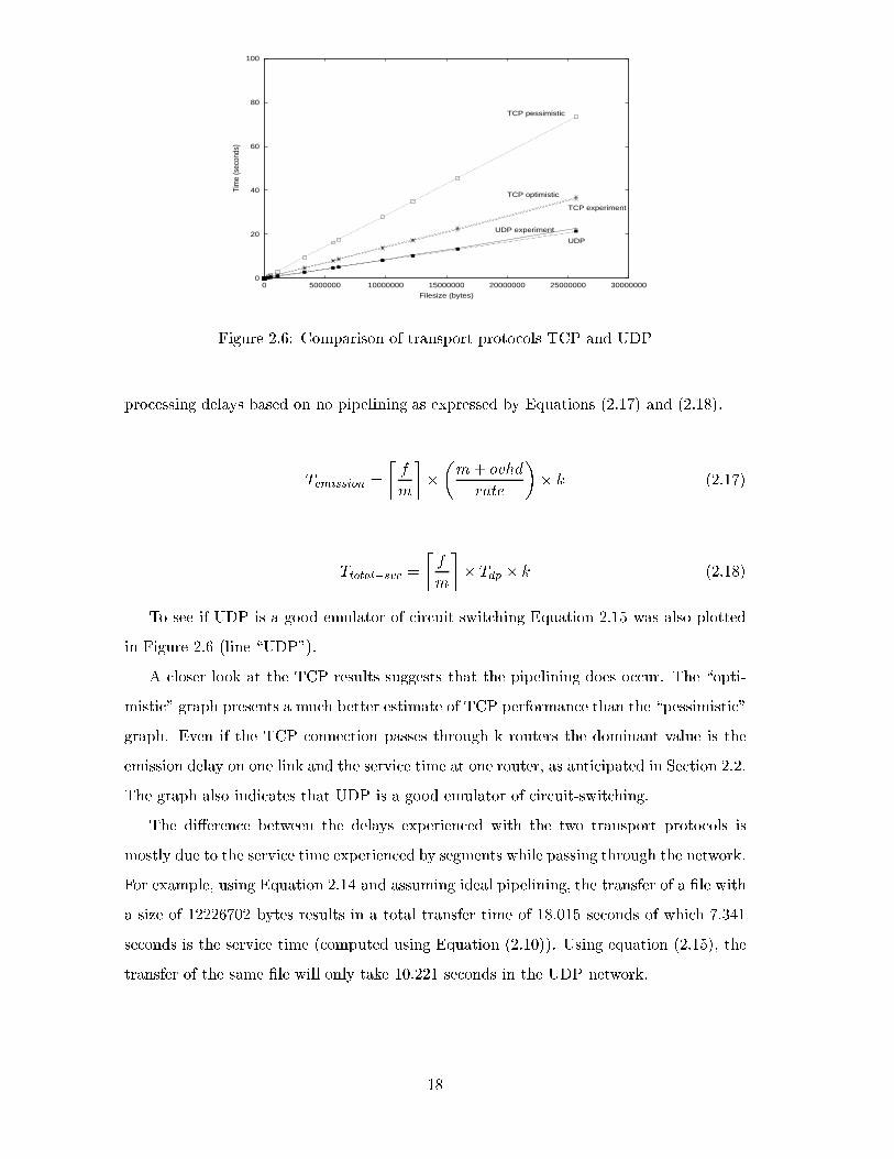
Figure 2.6 shows the results for di�erent �le sizes f given in Table 2.1, ranging from 13 to
25661582 bytes, and the corresponding experiments done to compare the predicted values
16
File sizes (bytes)
13
1205
4820
5898
14460
24796
62039
332008
544541
1091306
3309132
5654721
6120664
9731180
12226702
15918652
25661582
Table 2.1: Values used for �le sizes (f) in comparison of circuit-switching and TCP/IP
against real world tests. In the TCP tests, the number of routers (k) is 2, the message
size (m) is 1024 bytes and the overhead (ovhd) is 58 bytes (per message of size m). In the
UDP tests, the overhead (ovhd) is 46 bytes per segment.
In the graph (Figure 2.6) the predicted values (using our mathematical models) for
TCP/IP are also plotted. To predict the �le transfer delay using TCP/IP, we attempted
to provide bounds for the experimental results by computing the �le transfer delay under
the assumptions of ideal pipelining (\optimistic") and no pipelining (\pessimistic"). Both
the optimistic and the pessimistic graphs were plotted using Equations (2.12), (2.13) and
(2.14). The di�erence between the graphs is in how the emission and processing delays
(the terms Ttotal�svc and Temission from Equation (2.14)) are computed. In the optimistic
graph the emission and processing delays are based on ideal pipelining and expressed by
Equations (2.9) and (2.10) respectively. The pessimistic graph represents the emission and
17
0
20
40
60
80
100
0 5000000 10000000 15000000 20000000 25000000 30000000
Tim
e (s
econ
ds)
Filesize (bytes)
UDP experiment
TCP experiment
TCP optimistic
TCP pessimistic
UDP
Figure 2.6: Comparison of transport protocols TCP and UDP
processing delays based on no pipelining as expressed by Equations (2.17) and (2.18).
Temission =
�f
m
��
�m+ ovhd
rate
�� k (2.17)
Ttotal�svc =
�f
m
�� Tdp � k (2.18)
To see if UDP is a good emulator of circuit-switching Equation 2.15 was also plotted
in Figure 2.6 (line \UDP").
A closer look at the TCP results suggests that the pipelining does occur. The \opti-
mistic" graph presents a much better estimate of TCP performance than the \pessimistic"
graph. Even if the TCP connection passes through k routers the dominant value is the
emission delay on one link and the service time at one router, as anticipated in Section 2.2.
The graph also indicates that UDP is a good emulator of circuit-switching.
The di�erence between the delays experienced with the two transport protocols is
mostly due to the service time experienced by segments while passing through the network.
For example, using Equation 2.14 and assuming ideal pipelining, the transfer of a �le with
a size of 12226702 bytes results in a total transfer time of 18.015 seconds of which 7.341
seconds is the service time (computed using Equation (2.10)). Using equation (2.15), the
transfer of the same �le will only take 10.221 seconds in the UDP network.
18
2.4.4 The analytical results
The laboratory did not allow much freedom to note the behaviour of the two transport
protocols under operational conditions where large propagation delays might occur or a
large number of routers might be in place (for analysis of emission delays in TCP/IP).
Nevertheless, the experimental results from the previous section suggest that our equations
provide a good estimate of the delay we can expect when a �le is transferred using TCP/IP
and a circuit-switched network. Thus, we continue to apply our equations with variables
that indicate di�erent network conditions and con�gurations. This allows us to compare
the performance of TCP/IP to circuit switching more thoroughly.
The two network conditions of most interest are large propagation delays and large
emission delays (large number of hops in a TCP/IP network). In a TCP/IP network,
large propagation delays typically coincide with many hops. To divide the contributions
made to the total delay by the propagation and emission delays respectively, two scenar-
ios are explored and the behaviour of TCP/IP and circuit-switching in each scenario is
examined. Firstly, a network with large propagation delays, but few intermediate hops
was investigated. Secondly, a network with a large number of hops, but a relative smaller
propagation delay was used.
The baseline for these analytical investigations was obtained from the following ex-
periments. Testing with traceroute and ping revealed that the average round trip time
between a certain machine in the USA and a certain machine in Europe is 554.5 ms.
Another traceroute test between a machine in the USA and a machine in South Africa
revealed a hop count of 22.
The same round trip time and number of hops is assumed in the circuit switching and
TCP/IP computations. It is assumed that circuit switching is done with SONET (thus
introducing a 4.4% overhead). The same rate of 10Mbps is also assumed in the formulae
for computing circuit switching and TCP/IP times. It is assumed that 100ms of queueing
and processing (parameter Tproc from Equation (2.2)) is required at each circuit switch to
be able to set up a connection.
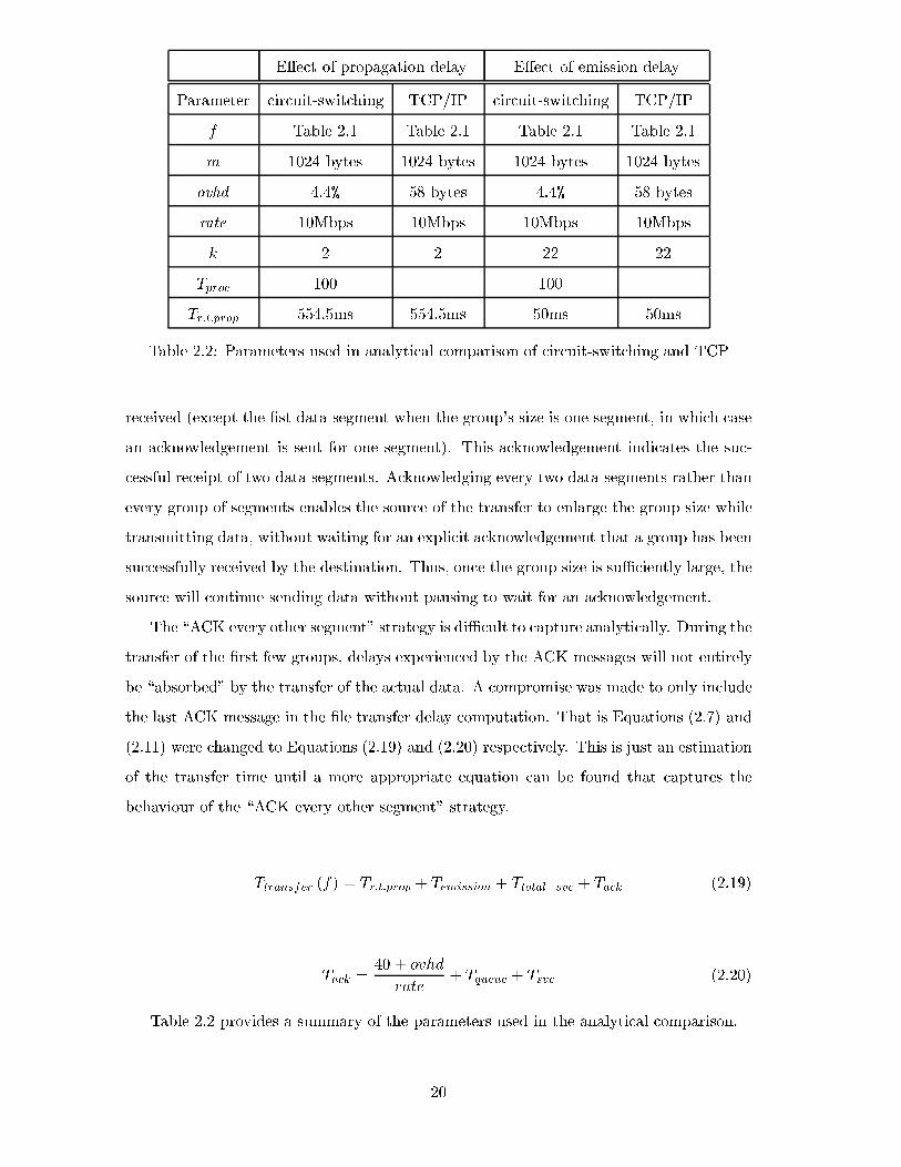
In each scenario the analysis of TCP was conducted for two implementations. In the
�rst implementation there is only one ACK sent for each group of segments (using Equa-
tion (2.7)). The second implementation considered was the \ACK every other segment"
strategy commonly used in TCP implementations. When making use of this strategy, the
destination of a �le transfer sends an acknowledgement for every second data segment
19
E�ect of propagation delay E�ect of emission delay
Parameter circuit-switching TCP/IP circuit-switching TCP/IP
f Table 2.1 Table 2.1 Table 2.1 Table 2.1
m 1024 bytes 1024 bytes 1024 bytes 1024 bytes
ovhd 4.4% 58 bytes 4.4% 58 bytes
rate 10Mbps 10Mbps 10Mbps 10Mbps
k 2 2 22 22
Tproc 100 100
Tr:t:prop 554.5ms 554.5ms 50ms 50ms
Table 2.2: Parameters used in analytical comparison of circuit-switching and TCP
received (except the �st data segment when the group's size is one segment, in which case
an acknowledgement is sent for one segment). This acknowledgement indicates the suc-
cessful receipt of two data segments. Acknowledging every two data segments rather than
every group of segments enables the source of the transfer to enlarge the group size while
transmitting data, without waiting for an explicit acknowledgement that a group has been
successfully received by the destination. Thus, once the group size is suÆciently large, the
source will continue sending data without pausing to wait for an acknowledgement.
The \ACK every other segment" strategy is diÆcult to capture analytically. During the
transfer of the �rst few groups, delays experienced by the ACK messages will not entirely
be \absorbed" by the transfer of the actual data. A compromise was made to only include
the last ACK message in the �le transfer delay computation. That is Equations (2.7) and
(2.11) were changed to Equations (2.19) and (2.20) respectively. This is just an estimation
of the transfer time until a more appropriate equation can be found that captures the
behaviour of the \ACK every other segment" strategy.
Ttransfer (f) = Tr:t:prop + Temission + Ttotal�svc + Tack (2.19)
Tack =40 + ovhd
rate+ Tqueue + Tsvc (2.20)
Table 2.2 provides a summary of the parameters used in the analytical comparison.
20
0
5
10
15
20
25
30
35
40
45
50
0 5000000 10000000 15000000 20000000 25000000 30000000 35000000
Tim
e (s
econ
ds)
Filesize (bytes)
Circuit switchingTCP ack every group
TCP ack 2nd segment
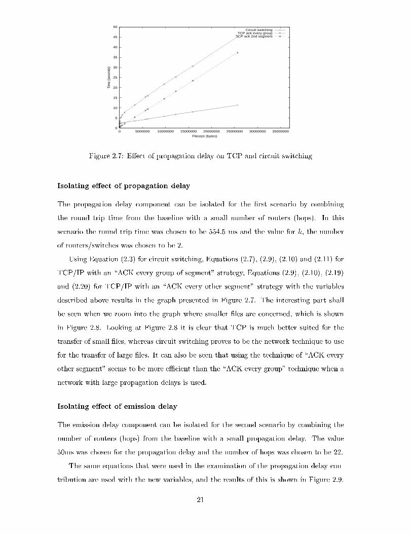
Figure 2.7: E�ect of propagation delay on TCP and circuit switching
Isolating e�ect of propagation delay
The propagation delay component can be isolated for the �rst scenario by combining
the round trip time from the baseline with a small number of routers (hops). In this
scenario the round trip time was chosen to be 554.5 ms and the value for k, the number
of routers/switches was chosen to be 2.
Using Equation (2.3) for circuit switching, Equations (2.7), (2.9), (2.10) and (2.11) for
TCP/IP with an \ACK every group of segment" strategy, Equations (2.9), (2.10), (2.19)
and (2.20) for TCP/IP with an \ACK every other segment" strategy with the variables
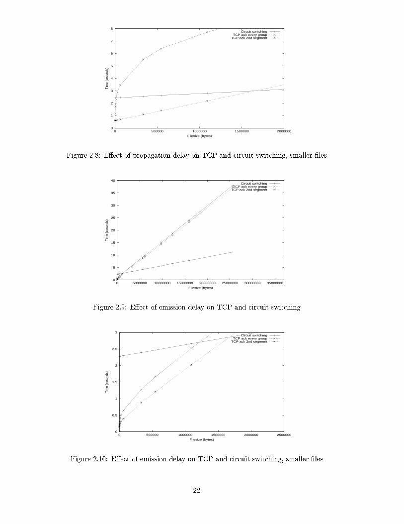
described above results in the graph presented in Figure 2.7. The interesting part shall
be seen when we zoom into the graph where smaller �les are concerned, which is shown
in Figure 2.8. Looking at Figure 2.8 it is clear that TCP is much better suited for the
transfer of small �les, whereas circuit switching proves to be the network technique to use
for the transfer of large �les. It can also be seen that using the technique of \ACK every
other segment" seems to be more eÆcient than the \ACK every group" technique when a
network with large propagation delays is used.
Isolating e�ect of emission delay
The emission delay component can be isolated for the second scenario by combining the
number of routers (hops) from the baseline with a small propagation delay. The value
50ms was chosen for the propagation delay and the number of hops was chosen to be 22.
The same equations that were used in the examination of the propagation delay con-
tribution are used with the new variables, and the results of this is shown in Figure 2.9.
21
0
1
2
3
4
5
6
7
8
0 500000 1000000 1500000 2000000
Tim
e (s
econ
ds)
Filesize (bytes)
Circuit switchingTCP ack every group
TCP ack 2nd segment
Figure 2.8: E�ect of propagation delay on TCP and circuit switching, smaller �les
0
5
10
15
20
25
30
35
40
0 5000000 10000000 15000000 20000000 25000000 30000000 35000000
Tim
e (s
econ
ds)
Filesize (bytes)
Circuit switchingTCP ack every group
TCP ack 2nd segment
Figure 2.9: E�ect of emission delay on TCP and circuit switching
0
0.5
1
1.5
2
2.5
3
0 500000 1000000 1500000 2000000 2500000
Tim
e (s
econ
ds)
Filesize (bytes)
Circuit switchingTCP ack every group
TCP ack 2nd segment
Figure 2.10: E�ect of emission delay on TCP and circuit switching, smaller �les
22
Again, a section of the graph is shown in Figure 2.10. The point at which the emission
delay when using TCP/IP becomes more signi�cant than the call setup delay in circuit
switching can be seen clearly in Figure 2.10. Sending any �le larger than the �le size at
that point (just over 1GB) with circuit switching will result in smaller delays than using
TCP/IP.
2.5 Conclusion
Queueing delays has changed over the years. In particular with the introduction of di�er-
entiated services it became necessary that all packet classi�cation actions be performed
at \wire speed" [8]. Thus, the processing of incoming packets has become fast enough
to keep up with the rate of incoming packets. Queueing delay is instead incurred at the
output port where the link insertion time and the number of packets destined for that link
determine the queueing delay. An analysis of the contribution of queueing delay to the
total delay is absent in the foregoing investigation. However such an analysis is unlikely
to a�ect the broad conclusions to be drawn from the investigation. This is because the
impact of queueing delay in circuit-switched networks is only present during connection
setup. During data transfer, all data is switched without experiencing queueing delay. On
the other hand, queueing delay will always contribute to the delay experienced by data
transfers over CL packet-switched networks.
Thus the evidence we have seen generally suggests that circuit switching is better suited
for large �le transfers than TCP. Using TCP, emission, propagation and queueing delay
all contribute signi�cantly to the total delay when a large �le is transferred . Propagation
delay and call setup time does contribute to the total delay experienced when a large �le
is transferred using circuit switching. The result of interest is the fact that there is always
a certain �le size, that serves as the dividing marker between TCP and circuit switching.
Transferring any �le larger than this size using circuit switching will result in transfer
speeds faster than if TCP was used.
The need for transferring large �les increases every day. Workstations are current-
ly equipped with more storage space than would have been imagined a few years ago.
There has also been an increase in the number of large �le transfers over the internet.
The increase is caused, for example, by the increase in occurrence of multimedia content
available for free and by the availability of large software packages for download over the
internet. Continuing this trend, the need to use circuit-switching will come to the fore
23

more forcefully. However, as pointed out at the start of this chapter, circuit switching as
a strategy can only succeed in an environment that provides high-bandwidth on-demand
circuits. Chapter 3 will propose a potential way of achieving this, based on appropriate
original protocols.
24
Chapter 3
Signaling protocol
3.1 Introduction
Chapter 2Analyzing file transfer delays in
circuit-switched and TCP/IP networks.
Chapter 6Further work:
Transport layer
Chapter 3
Signaling protocol
Chapter 5Scheduling calls with known holding times
Chapter 4
Routing protocol
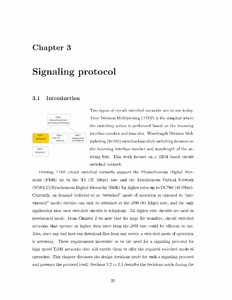
Two types of circuit switched networks are in use today.
Time Division Multiplexing (TDM) is the simplest where
the switching action is performed based on the incoming
interface number and time slot. Wavelength Division Mul-
tiplexing (WDM) switches base their switching decision on
the incoming interface number and wavelength of the ar-
riving bits. This work focuses on a TDM based circuit
switched network.
Existing TDM circuit switched networks support the Plesiochronous Digital Hier-
archy (PDH) up to the T3 (45 Mbps) rate and the Synchronous Optical Network
(SONET)/Synchronous Digital Hierarchy (SDH) for higher rates up to OC768 (40 Gbps).
Currently, on demand (referred to as \switched" mode of operation as opposed to \pro-
visioned" mode) circuits can only be obtained at the DS0 (64 Kbps) rate, and the only
application that uses switched circuits is telephony. All higher rate circuits are used in
provisioned mode. From Chapter 2 we note that for large �le transfers, circuit switched
networks that operate at higher data rates than the DS0 rate could be eÆcient to use.
Also, since any end host can download �les from any server, a switched mode of operation
is necessary. These requirements introduce us to the need for a signaling protocol for
high speed TDM networks that will enable them to o�er the required switched mode of
operation. This chapter discusses the design decisions made for such a signaling protocol
and presents the protocol itself. Sections 3.2 to 3.4 describe the decisions made during the
25
design of the signaling protocol and an overview of the protocol itself. Sections 3.5 to 3.8
explain the protocol speci�cation, and Section 3.9 introduces some future improvements
to the signaling protocol.
3.2 Implementing the signaling protocol in hardware
One of the early decisions we made before designing the signaling protocol was to imple-
ment the protocol in hardware. Typically signaling protocols are implemented in software
due to the complexity of the protocols and the need to keep the implementation ex-
ible for evolution reasons. On the other hand, hardware implementations would yield
a performance improvement so signi�cant that the role and use of high speed circuit
switched networks would change dramatically. To obtain such a performance gain while
retaining some exibility we recommend the use of recon�gurable hardware such as Field
Programmable Gate Arrays (FPGAs).
Hardware implementations of networking protocols are on the rise. It has been quite
common to implement physical-layer and data-link layer protocols in hardware. For ex-
ample, Ethernet chips have been available for a long time for use in network interface
cards. An Ethernet chip in a network interface card plugged into a host (workstation or
pc) simply performs a 6 byte (MAC) address matching function. Chips are also avail-
able to perform Ethernet switching, where frames are switched on their destination MAC
addresses.
Moving up the protocol stack, network-layer protocols are now being implemented
in hardware. First, chipsets were created for ATM header processing as well as ATM
switching. ATM is the network-layer protocol of a packet-switched Connection-Oriented
(CO) network. In such networks, since a connection is �rst set up, the identi�ers on
which the switching is performed are simpler than in a packet-switched connectionless
network-layer protocol, where switching is performed on destination addresses as in IP.
More recently, network-layer protocols for even connectionless networks, such as IP, are
being implemented in hardware. The throughput of IP routers (now called IP \switches")
is greatly improved with hardware implementations. Also, the latency incurred per packet,
which includes queueing and processing delays at each switch, is reduced. Thus there are
many advantages to hardware implementations of networking protocols. Loss of exibility
as protocols are upgraded is cited as the main drawback of hardware implementations.
However, now with recon�gurable hardware, this drawback should no longer be a serious
26
concern. It is also feasible to use hardware only for the basic operations of the protocol
and relegate more complex and infrequent operations (for example, processing of options
�elds in the IP header) to software.
All of the protocols discussed above are used to carry user data, and are hence re-
ferred to as \user-plane" protocols. Our interest is in applying this same technique of
improving performance through hardware implementations to \control-plane" protocols.
Signaling protocols are control-plane protocols used to set up and release connections.
These protocols are only needed in CO networks.
Current implementations of signaling protocols for both circuit-switched and packet-
switched CO networks are done in software. Call setup signaling messages are queued
at processors associated with switches and handled typically on a �rst-come-�rst-serve
basis. Queueing delays are incurred under moderate and heavy load conditions. These
delays add up across the switches dominating propagation delays and causing end-to-
end call setup delays to be signi�cant. Also, the processors handling signaling messages
often become bottlenecks [2]-[4]. Hardware implementations of signaling protocols will
greatly help improve both call setup delays and call handling capacities. By implementing
the signaling protocol in hardware the throughput will increase signi�cantly, thus a CO
network will be able to admit more connections in a time period.
There are many challenges to implementing signaling protocols in hardware that have
not been encountered in hardware implementations of user-plane protocols. The main
di�erence is that in handling signaling protocols, the hardware needs to maintain state
information of connections, whereas all the user-plane protocols implemented in hardware
are stateless. Ethernet frames, ATM cells and IP datagrams are simply forwarded without
any state being maintained for each packet or \ ow".
The work items to provide a practical environment for such a signaling protocol include:
1. speci�cation of a signaling protocol
2. implementation of the signaling protocol in hardware (using FPGAs)
3. design and analysis of how these signaling protocol chips can be used in a switch
controller, and
4. design and analysis of end-to-end applications that can use high bandwidth on-
demand circuits.
27
Circuit Circuit Circuitswitch switch switch
End hostA
End host
B
Figure 3.1: Ideal network in which signaling protocol will be used
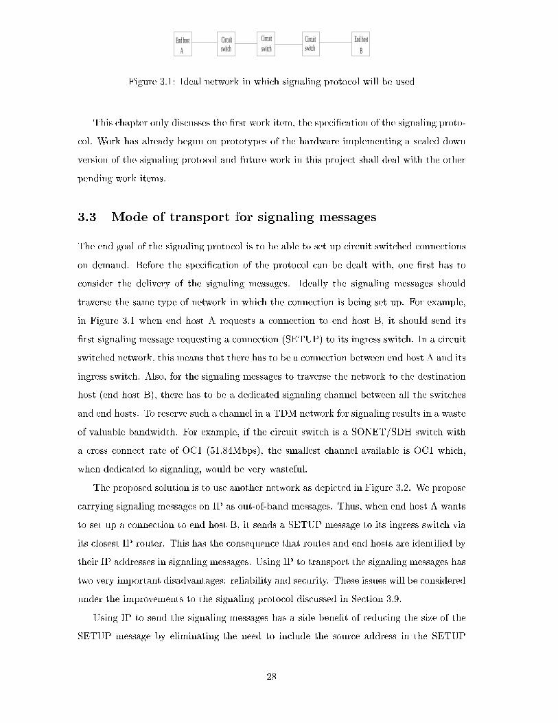
This chapter only discusses the �rst work item, the speci�cation of the signaling proto-
col. Work has already begun on prototypes of the hardware implementing a scaled down
version of the signaling protocol and future work in this project shall deal with the other
pending work items.
3.3 Mode of transport for signaling messages
The end goal of the signaling protocol is to be able to set up circuit switched connections
on demand. Before the speci�cation of the protocol can be dealt with, one �rst has to
consider the delivery of the signaling messages. Ideally the signaling messages should
traverse the same type of network in which the connection is being set up. For example,
in Figure 3.1 when end host A requests a connection to end host B, it should send its
�rst signaling message requesting a connection (SETUP) to its ingress switch. In a circuit
switched network, this means that there has to be a connection between end host A and its
ingress switch. Also, for the signaling messages to traverse the network to the destination
host (end host B), there has to be a dedicated signaling channel between all the switches
and end hosts. To reserve such a channel in a TDM network for signaling results in a waste
of valuable bandwidth. For example, if the circuit switch is a SONET/SDH switch with
a cross connect rate of OC1 (51.84Mbps), the smallest channel available is OC1 which,
when dedicated to signaling, would be very wasteful.
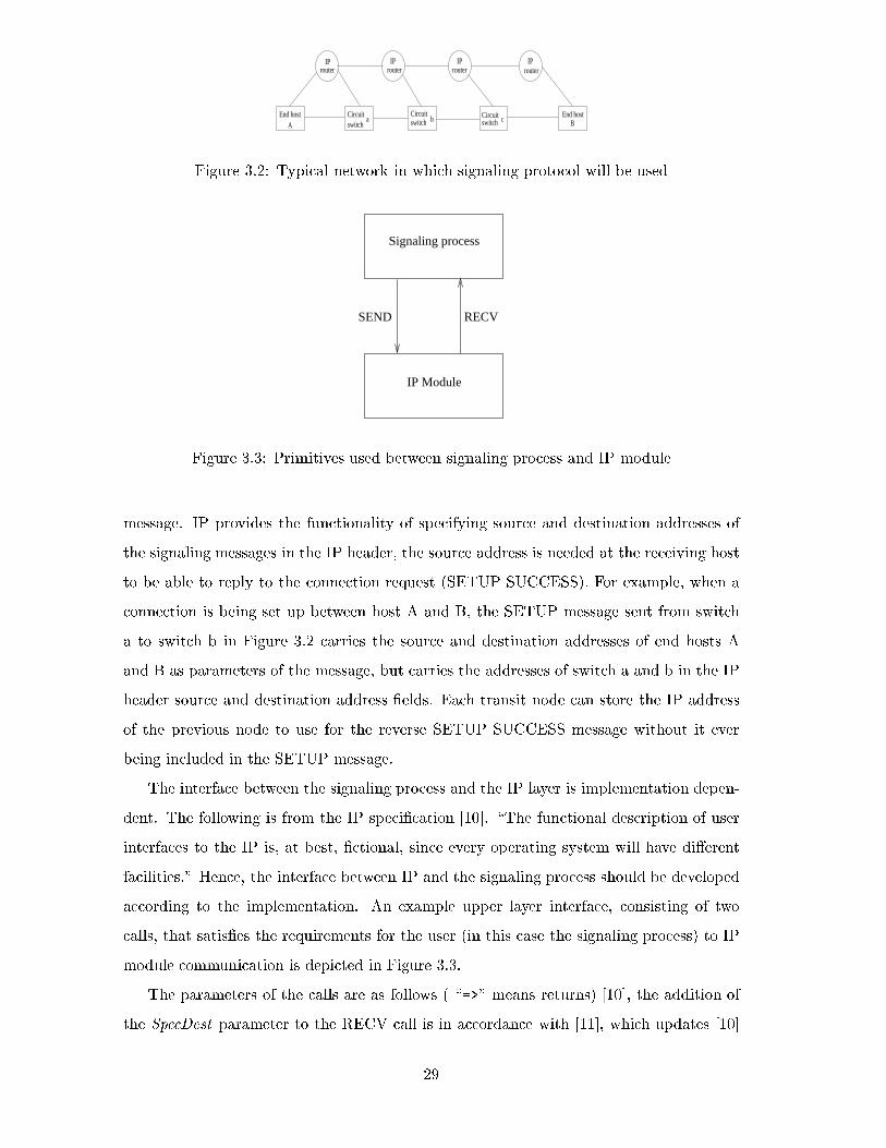
The proposed solution is to use another network as depicted in Figure 3.2. We propose
carrying signaling messages on IP as out-of-band messages. Thus, when end host A wants
to set up a connection to end host B, it sends a SETUP message to its ingress switch via
its closest IP router. This has the consequence that routes and end hosts are identi�ed by
their IP addresses in signaling messages. Using IP to transport the signaling messages has
two very important disadvantages: reliability and security. These issues will be considered
under the improvements to the signaling protocol discussed in Section 3.9.
Using IP to send the signaling messages has a side bene�t of reducing the size of the
SETUP message by eliminating the need to include the source address in the SETUP
28
IP IP IP IProuterrouterrouterrouter
End hostA
End hostB
Circuitswitch switch
Circuit Circuitswitcha b c
Figure 3.2: Typical network in which signaling protocol will be used
SEND RECV
Signaling process
IP Module
Figure 3.3: Primitives used between signaling process and IP module
message. IP provides the functionality of specifying source and destination addresses of
the signaling messages in the IP header, the source address is needed at the receiving host
to be able to reply to the connection request (SETUP SUCCESS). For example, when a
connection is being set up between host A and B, the SETUP message sent from switch
a to switch b in Figure 3.2 carries the source and destination addresses of end hosts A
and B as parameters of the message, but carries the addresses of switch a and b in the IP
header source and destination address �elds. Each transit node can store the IP address
of the previous node to use for the reverse SETUP SUCCESS message without it ever
being included in the SETUP message.
The interface between the signaling process and the IP layer is implementation depen-
dent. The following is from the IP speci�cation [10]. \The functional description of user
interfaces to the IP is, at best, �ctional, since every operating system will have di�erent
facilities." Hence, the interface between IP and the signaling process should be developed
according to the implementation. An example upper layer interface, consisting of two
calls, that satis�es the requirements for the user (in this case the signaling process) to IP
module communication is depicted in Figure 3.3.
The parameters of the calls are as follows ( \=>" means returns) [10], the addition of
the SpecDest parameter to the RECV call is in accordance with [11], which updates [10]
29
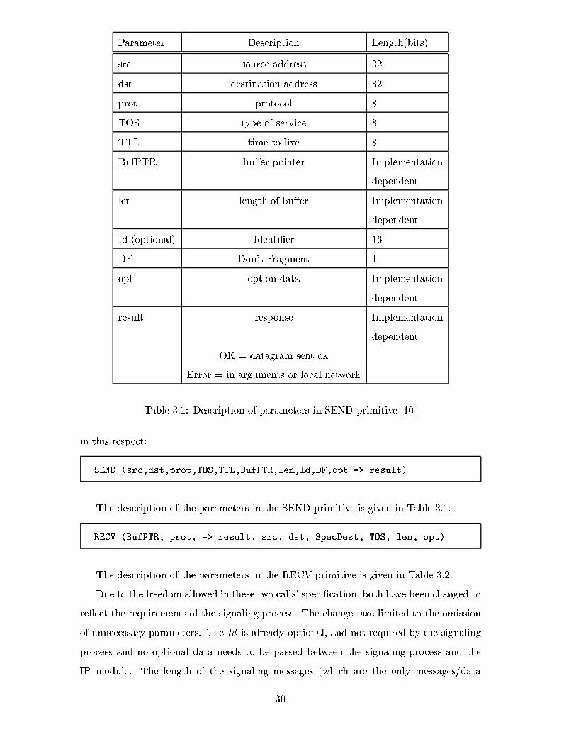
Parameter Description Length(bits)
src source address 32
dst destination address 32
prot protocol 8
TOS type of service 8
TTL time to live 8
BufPTR bu�er pointer Implementation
dependent
len length of bu�er Implementation
dependent
Id (optional) Identi�er 16
DF Don't Fragment 1
opt option data Implementation
dependent
result response Implementation
dependent
OK = datagram sent ok
Error = in arguments or local network
Table 3.1: Description of parameters in SEND primitive [10]
in this respect:
SEND (src,dst,prot,TOS,TTL,BufPTR,len,Id,DF,opt => result)
The description of the parameters in the SEND primitive is given in Table 3.1.
RECV (BufPTR, prot, => result, src, dst, SpecDest, TOS, len, opt)
The description of the parameters in the RECV primitive is given in Table 3.2.
Due to the freedom allowed in these two calls' speci�cation, both have been changed to
re ect the requirements of the signaling process. The changes are limited to the omission
of unnecessary parameters. The Id is already optional, and not required by the signaling
process and no optional data needs to be passed between the signaling process and the
IP module. The length of the signaling messages (which are the only messages/data
30
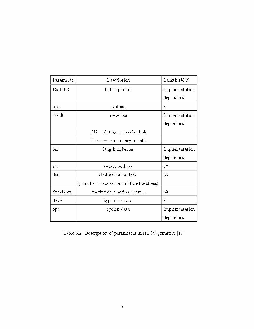
Parameter Description Length (bits)
BufPTR bu�er pointer Implementation
dependent
prot protocol 8
result response Implementation
dependent
OK = datagram received ok
Error = error in arguments
len length of bu�er Implementation
dependent
src source address 32
dst destination address 32
(may be broadcast or multicast address)
SpecDest speci�c destination address 32
TOS type of service 8
opt option data Implementation
dependent
Table 3.2: Description of parameters in RECV primitive [10]
31
passed between the signaling process and the IP module) is either included in the signaling
message itself, or it can be deduced from the message type. This eliminates the need for
the IP module to include the length of the message when it is passed to the signaling
process (the RECV primitive). The remaining parameters have the same description and
length as before. The SEND call has been changed to:
SEND (src,dst,prot,TOS,TTL,BufPTR,len,DF => result)
The RECV call have been changed to the following:
RECV (BufPTR, prot, => result, src, dst, SpecDest)
Other implementation decisions are:
� The Type of Service (TOS) parameter indicates to the IP network the quality of
service desired for the data transfer. It shall always be set to 0001 0100 which
indicates a request for low delay and high reliability when a signaling message is
transferred.
� The len parameter will be a 16 bit value that is an exact copy of the message length
information element in the SETUP message. For all the other messages, it shall
contain the length of the signaling message.
� The usage of two destination address parameters (dst and SpecDest) in the RECV
call is required due to the IP facility for broadcasting and multicasting. The speci�c-
destination address (SpecDest) is de�ned to be the destination address (dst) in the
IP header unless the header contains a broadcast or multicast address, in which case
the speci�c-destination is an IP address assigned to the physical interface on which
the datagram arrived [11]. No signaling message should be destined for a multicast
group or sent as a broadcast message over the network. For this reason, the signaling
message shall immediately be discarded when the two destination parameters are not
equal.
� Use 8 bits for the result parameter, and the value 200 shall indicate success.
� The protocol value of 253 will be used to indicate the signaling layer. This value is
currently unassigned according to [21].
32
� When data is passed to the IP layer, the TTL parameter will always be set to 16.
This number indicates the maximum acceptable number of routers between TDM
switches.
� The DF parameter shall always be set to 1, which indicates that this message may
not be fragmented by the IP network. This is because the maximum size for the
SETUP message is 407 bytes and given that the IP speci�cation, [10], dictates that
all hosts must be prepared to accept datagrams of up to 576 bytes, the message will
never need to be fragmented by the IP network (even if a maximum sized header is
included in the datagram).
3.4 Signaling protocol description
This signaling protocol is intended to be used in a circuit-switched CO network where
connections are used for large �le transfers, which have been proven to be the ideal appli-
cation for high speed circuit-switched CO networks. Also, in a quest for a simple design
of this protocol, a homogeneous network (where all the switches operate at the same cross
connect rate) is assumed to be the target network. Changes to the signaling protocol when
it is used in a heterogenous network will be discussed under the improvements to the sig-
naling protocol in Section 3.9. With the above implementation considerations, certain
assumptions can be made in the design of this protocol. They are:
� Only unidirectional two-party connections are allowed. The reason for this is that
the primary application is large �le transfers. Connections would then primarily be
needed to transfer a large �le from a server to a client.
� The setup requests are generated by the sending end of the unidirectional connec-
tions.
� The bandwidth requested in a SETUP message is either equal to, or an integral
multiple of the (homogeneous network) switch cross connect rate. The bandwidth
can be requested with the speci�cation of a range that indicates minimum and max-
imum bandwidth requirements. Using these two parameters, the network attempts
to allocate the maximum requested bandwidth. If any node along the path of the
connection cannot provide the requested bandwidth, the highest bandwidth less than
the maximum requested and larger or equal to the minimum requested is reserved.
33
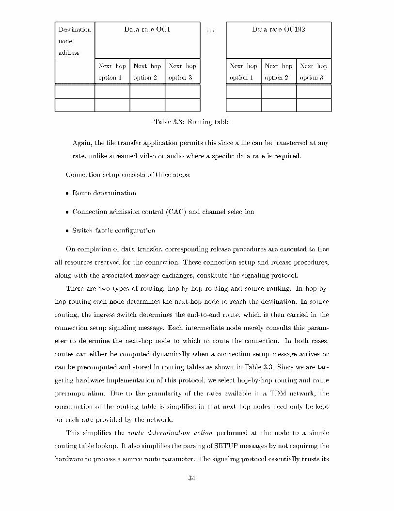
Destination
node
address
Data rate OC1 : : : Data rate OC192
Next hop
option 1
Next hop
option 2
Next hop
option 3
Next hop
option 1
Next hop
option 2
Next hop
option 3
Table 3.3: Routing table
Again, the �le transfer application permits this since a �le can be transferred at any
rate, unlike streamed video or audio where a speci�c data rate is required.
Connection setup consists of three steps:
� Route determination
� Connection admission control (CAC) and channel selection
� Switch fabric con�guration
On completion of data transfer, corresponding release procedures are executed to free
all resources reserved for the connection. These connection setup and release procedures,
along with the associated message exchanges, constitute the signaling protocol.
There are two types of routing, hop-by-hop routing and source routing. In hop-by-
hop routing each node determines the next-hop node to reach the destination. In source
routing, the ingress switch determines the end-to-end route, which is then carried in the
connection setup signaling message. Each intermediate node merely consults this param-
eter to determine the next-hop node to which to route the connection. In both cases,
routes can either be computed dynamically when a connection setup message arrives or
can be precomputed and stored in routing tables as shown in Table 3.3. Since we are tar-
geting hardware implementation of this protocol, we select hop-by-hop routing and route
precomputation. Due to the granularity of the rates available in a TDM network, the
construction of the routing table is simpli�ed in that next hop nodes need only be kept
for each rate provided by the network.
This simpli�es the route determination action performed at the node to a simple
routing table lookup. It also simpli�es the parsing of SETUP messages by not requiring the
hardware to process a source route parameter. The signaling protocol essentially trusts its
34
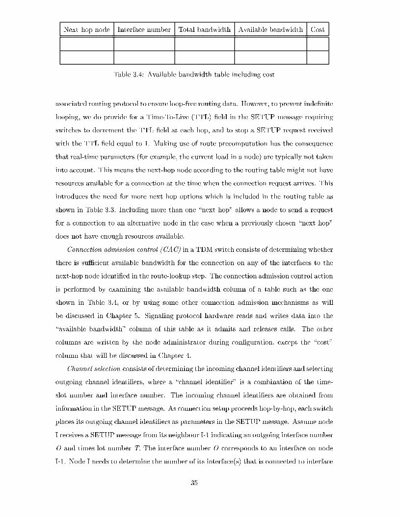
Next hop node Interface number Total bandwidth Available bandwidth Cost
Table 3.4: Available bandwidth table including cost
associated routing protocol to ensure loop-free routing data. However, to prevent inde�nite
looping, we do provide for a Time-To-Live (TTL) �eld in the SETUP message requiring
switches to decrement the TTL �eld at each hop, and to stop a SETUP request received
with the TTL �eld equal to 1. Making use of route precomputation has the consequence
that real-time parameters (for example, the current load in a node) are typically not taken
into account. This means the next-hop node according to the routing table might not have
resources available for a connection at the time when the connection request arrives. This
introduces the need for more next hop options which is included in the routing table as
shown in Table 3.3. Including more than one \next hop" allows a node to send a request
for a connection to an alternative node in the case when a previously chosen \next hop"
does not have enough resources available.
Connection admission control (CAC) in a TDM switch consists of determining whether
there is suÆcient available bandwidth for the connection on any of the interfaces to the
next-hop node identi�ed in the route-lookup step. The connection admission control action
is performed by examining the available bandwidth column of a table such as the one
shown in Table 3.4, or by using some other connection admission mechanisms as will
be discussed in Chapter 5. Signaling protocol hardware reads and writes data into the
\available bandwidth" column of this table as it admits and releases calls. The other
columns are written by the node administrator during con�guration, except the \cost"
column that will be discussed in Chapter 4.
Channel selection consists of determining the incoming channel identi�ers and selecting
outgoing channel identi�ers, where a \channel identi�er" is a combination of the time-
slot number and interface number. The incoming channel identi�ers are obtained from
information in the SETUPmessage. As connection setup proceeds hop-by-hop, each switch
places its outgoing channel identi�ers as parameters in the SETUP message. Assume node
I receives a SETUPmessage from its neighbour I-1 indicating an outgoing interface number
O and times lot number T. The interface number O corresponds to an interface on node
I-1. Node I needs to determine the number of its interface(s) that is connected to interface
35
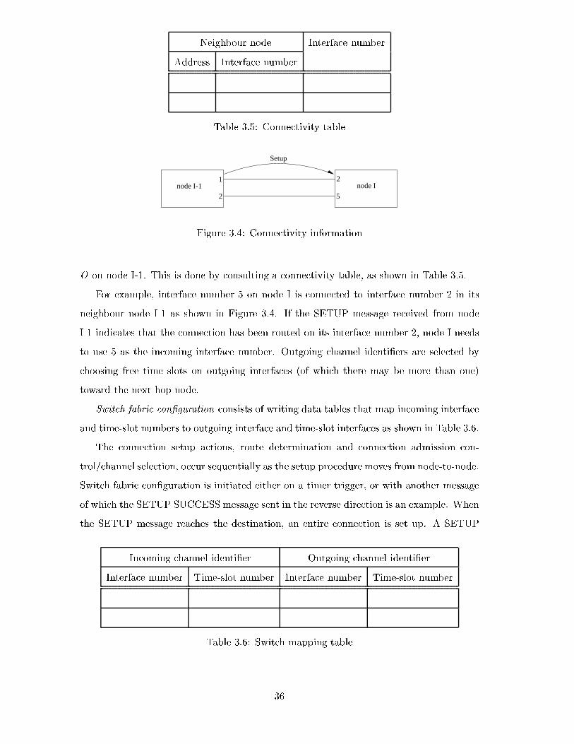
Neighbour node Interface number
Address Interface number
Table 3.5: Connectivity table
node Inode I-11
2
2
5
Setup
Figure 3.4: Connectivity information
O on node I-1. This is done by consulting a connectivity table, as shown in Table 3.5.
For example, interface number 5 on node I is connected to interface number 2 in its
neighbour node I-1 as shown in Figure 3.4. If the SETUP message received from node
I-1 indicates that the connection has been routed on its interface number 2, node I needs
to use 5 as the incoming interface number. Outgoing channel identi�ers are selected by
choosing free time slots on outgoing interfaces (of which there may be more than one)
toward the next hop node.
Switch fabric con�guration consists of writing data tables that map incoming interface
and time-slot numbers to outgoing interface and time-slot interfaces as shown in Table 3.6.
The connection setup actions, route determination and connection admission con-
trol/channel selection, occur sequentially as the setup procedure moves from node-to-node.
Switch fabric con�guration is initiated either on a timer trigger, or with another message
of which the SETUP SUCCESS message sent in the reverse direction is an example. When
the SETUP message reaches the destination, an entire connection is set up. A SETUP
Incoming channel identi�er Outgoing channel identi�er
Interface number Time-slot number Interface number Time-slot number
Table 3.6: Switch mapping table
36
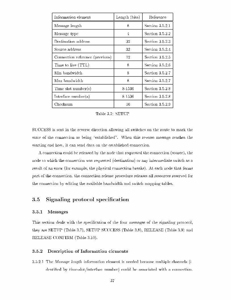
Information element Length (bits) Reference
Message length 8 Section 3.5.2.1
Message type 4 Section 3.5.2.2
Destination address 32 Section 3.5.2.3
Source address 32 Section 3.5.2.4
Connection reference (previous) 12 Section 3.5.2.5
Time to live (TTL) 8 Section 3.5.2.6
Min bandwidth 8 Section 3.5.2.7
Max bandwidth 8 Section 3.5.2.7
Time slot number(s) 8-1536 Section 3.5.2.8
Interface number(s) 8-1536 Section 3.5.2.8
Checksum 16 Section 3.5.2.9
Table 3.7: SETUP
SUCCESS is sent in the reverse direction allowing all switches on the route to mark the
state of the connection as being \established". When this reverse message reaches the
starting end host, it can send data on the established connection.
A connection could be released by the node that requested the connection (source), the
node to which the connection was requested (destination) or any intermediate switch as a
result of an error (for example, the physical connection breaks). At each node that forms
part of the connection, the connection release procedure releases all resources reserved for
the connection by editing the available bandwidth and switch mapping tables.
3.5 Signaling protocol speci�cation
3.5.1 Messages
This section deals with the speci�cation of the four messages of the signaling protocol,
they are SETUP (Table 3.7), SETUP SUCCESS (Table 3.8), RELEASE (Table 3.9) and
RELEASE CONFIRM (Table 3.10).
3.5.2 Description of Information elements
3.5.2.1 The Message length information element is needed because multiple channels (i-
denti�ed by time-slot/interface number) could be associated with a connection.
37
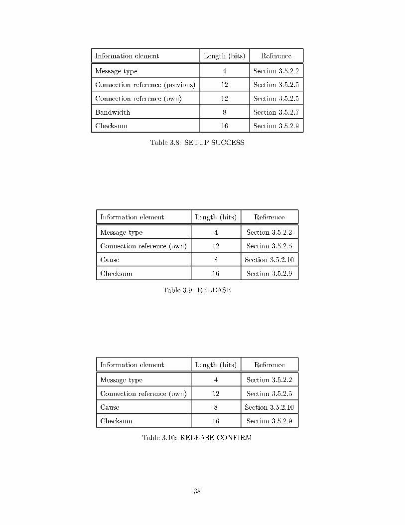
Information element Length (bits) Reference
Message type 4 Section 3.5.2.2
Connection reference (previous) 12 Section 3.5.2.5
Connection reference (own) 12 Section 3.5.2.5
Bandwidth 8 Section 3.5.2.7
Checksum 16 Section 3.5.2.9
Table 3.8: SETUP SUCCESS
Information element Length (bits) Reference
Message type 4 Section 3.5.2.2
Connection reference (own) 12 Section 3.5.2.5
Cause 8 Section 3.5.2.10
Checksum 16 Section 3.5.2.9
Table 3.9: RELEASE
Information element Length (bits) Reference
Message type 4 Section 3.5.2.2
Connection reference (own) 12 Section 3.5.2.5
Cause 8 Section 3.5.2.10
Checksum 16 Section 3.5.2.9
Table 3.10: RELEASE CONFIRM
38
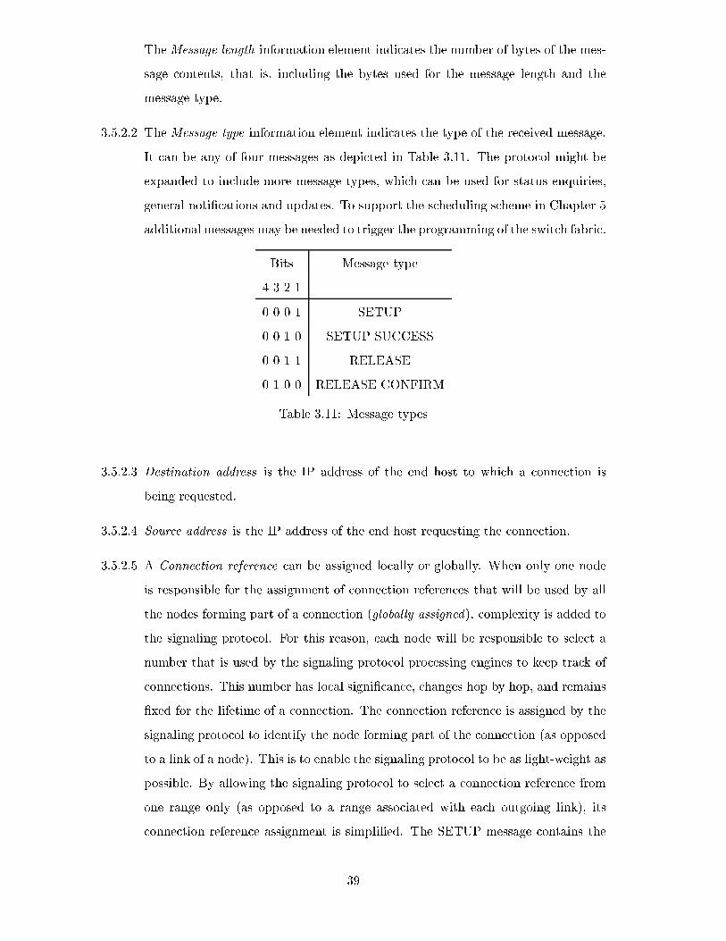
The Message length information element indicates the number of bytes of the mes-
sage contents, that is, including the bytes used for the message length and the
message type.
3.5.2.2 The Message type information element indicates the type of the received message.
It can be any of four messages as depicted in Table 3.11. The protocol might be
expanded to include more message types, which can be used for status enquiries,
general noti�cations and updates. To support the scheduling scheme in Chapter 5
additional messages may be needed to trigger the programming of the switch fabric.
Bits Message type
4 3 2 1
0 0 0 1 SETUP
0 0 1 0 SETUP SUCCESS
0 0 1 1 RELEASE
0 1 0 0 RELEASE CONFIRM
Table 3.11: Message types
3.5.2.3 Destination address is the IP address of the end host to which a connection is
being requested.
3.5.2.4 Source address is the IP address of the end host requesting the connection.
3.5.2.5 A Connection reference can be assigned locally or globally. When only one node
is responsible for the assignment of connection references that will be used by all
the nodes forming part of a connection (globally assigned), complexity is added to
the signaling protocol. For this reason, each node will be responsible to select a
number that is used by the signaling protocol processing engines to keep track of
connections. This number has local signi�cance, changes hop by hop, and remains
�xed for the lifetime of a connection. The connection reference is assigned by the
signaling protocol to identify the node forming part of the connection (as opposed
to a link of a node). This is to enable the signaling protocol to be as light-weight as
possible. By allowing the signaling protocol to select a connection reference from
one range only (as opposed to a range associated with each outgoing link), its
connection reference assignment is simpli�ed. The SETUP message contains the
39
connection reference being used by the node that sent the message. The RELEASE
and RELEASE CONFIRM messages contain the connection reference being used
by the node to which the message is sent. In reply to a SETUP message, the
SETUP SUCCESS message to the previous node contains the connection reference
of the node to which the message is being sent (which is the same as the one
included in the received SETUP message), and the connection reference reserved
for the connection by the node that sent the SETUP SUCCESS message. That
is, the SETUP SUCCESS message sent from node i to node i � 1 contains the
connection references assigned by node i and node i� 1.
3.5.2.6 The Time to live (TTL) information element is used to prevent inde�nite looping.
It is decremented at every node, and if it reaches the value 1 at any transit node
(which is any node except the end nodes), the setup is deemed a failure.
3.5.2.7 TheMin bandwidth andMax bandwidth information elements contain the minimum
and maximum bandwidths requested for the connection in the SETUP message.
The Bandwidth information element in the SETUP SUCCESS message contains
the bandwidth agreed on for the connection. These information elements should
contain the bandwidth in multiples of OC1 connections. Thus, when an OC48
connection is requested, the bandwidth (minimum and maximum) �eld shall con-
tain \00110000". This allows for a request for a connection with bandwidth of up
to OC192.
3.5.2.8 The time-slot number(s) and interface number(s) information elements contain
the values selected for the channels that will carry user data. Like connection
references, these numbers also change at each hop. We allow for multiple numbers
in case the requested bandwidth is greater than the switch cross connect rate.
3.5.2.9 A checksum information element allows for error checking on the received mes-
sage. If the checksum fails, the message is immediately discarded by the signaling
process.
3.5.2.10 The cause information element indicates to the receiver of a RELEASE or
RELEASE CONFIRM message the reason why the connection is being cleared.
These values can follow the messages as de�ned in ITU-T Recommendation Q.2610.
According to this recommendation, the information element has a variable length,
40
but we shall only need the de�nitions of the di�erent types of errors and their
respective values.
3.5.2.11 The Multi-tag parameter present bit indicates if the multi-path tag parameter is
present. It is set to 1 if the parameter is present.
3.5.3 Tables
The signaling protocol relies on the use of �ve tables, four of which have been discussed
in Section 3.4, they are:
1. Routing table, Table 3.3;
2. Available Bandwidth table, Table 3.4;
3. Connectivity table, Table 3.5;
4. Switch mapping table, Table 3.6; and
5. State table, Table 3.12.
The state of every connection being established, released, or in use is maintained both
at the end hosts and at the switches. The state diagram for the signaling protocol is as
shown in Figure 3.5. In the Setup received state, two of the connection setup actions are
performed. The third connection setup action (switch programming) is performed in the
Established state. In the Release received state, the release actions are performed.
A state table such as the one shown in Table 3.12 is updated each time a signaling
message is received. Since connection references are local, the connection references used
by the previous and next nodes forming part of the connection are stored in the state
table. The signaling protocol will always use the connection reference it assigned to the
node (own) as an index to this table.
The state entry indicates the state of each connection with a number assigned to each of
the states shown in Figure 3.5. The bandwidth, previous- and next-node address �elds are
maintained for each connection. The last column stores the outgoing channel identi�ers
of which there could be many per connection.
There are six states de�ned for this protocol. They are:
1. Closed No connection exits
41
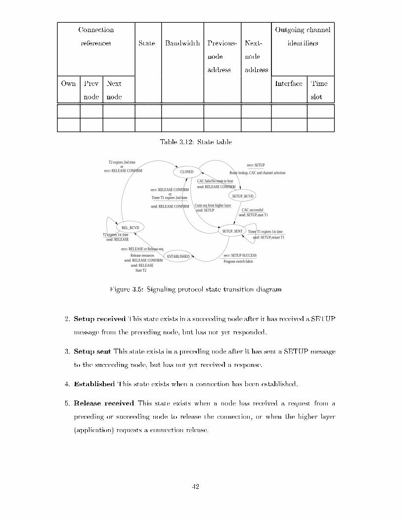
Connection Outgoing channel
references State Bandwidth Previous-
node
address
Next-
node
address
identi�ers
Own Prev
node
Next
node
Interface Time
slot
Table 3.12: State table
CLOSED
SETUP_RCVD
SETUP_SENT
ESTABLISHED
REL_RCVD
CAC fails/No route to host
Timer T1 expires 1st time
Conn req from higher layer
T2 expires 1st time
orT2 expires 2nd time
Program switch fabric
Route lookup, CAC and channel selection
send: SETUP,start T1
send: SETUP,restart T1
send: SETUP
recv: SETUP SUCCESS
send: RELEASE
recv: RELEASE CONFIRM
recv: RELEASE CONFIRMor
Timer T1 expires 2nd time
recv: RELEASE or Release-req
Release resourcessend: RELEASE CONFIRM
send: RELEASEStart T2
CAC successful
recv: SETUP
send: RELEASE CONFIRM
send: RELEASE CONFIRM
Figure 3.5: Signaling protocol state transition diagram
2. Setup received This state exists in a succeeding node after it has received a SETUP
message from the preceding node, but has not yet responded.
3. Setup sent This state exists in a preceding node after it has sent a SETUP message
to the succeeding node, but has not yet received a response.
4. Established This state exists when a connection has been established.
5. Release received This state exists when a node has received a request from a
preceding or succeeding node to release the connection, or when the higher layer
(application) requests a connection release.
42
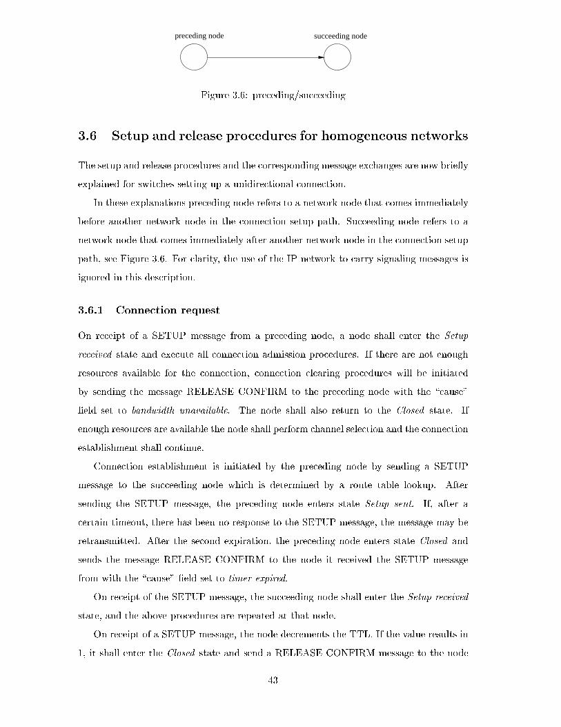
preceding node succeeding node
Figure 3.6: preceding/succeeding
3.6 Setup and release procedures for homogeneous networks
The setup and release procedures and the corresponding message exchanges are now brie y
explained for switches setting up a unidirectional connection.
In these explanations preceding node refers to a network node that comes immediately
before another network node in the connection setup path. Succeeding node refers to a
network node that comes immediately after another network node in the connection setup
path, see Figure 3.6. For clarity, the use of the IP network to carry signaling messages is
ignored in this description.
3.6.1 Connection request
On receipt of a SETUP message from a preceding node, a node shall enter the Setup
received state and execute all connection admission procedures. If there are not enough
resources available for the connection, connection clearing procedures will be initiated
by sending the message RELEASE CONFIRM to the preceding node with the \cause"
�eld set to bandwidth unavailable. The node shall also return to the Closed state. If
enough resources are available the node shall perform channel selection and the connection
establishment shall continue.
Connection establishment is initiated by the preceding node by sending a SETUP
message to the succeeding node which is determined by a route table lookup. After
sending the SETUP message, the preceding node enters state Setup sent. If, after a
certain timeout, there has been no response to the SETUP message, the message may be
retransmitted. After the second expiration, the preceding node enters state Closed and
sends the message RELEASE CONFIRM to the node it received the SETUP message
from with the \cause" �eld set to timer expired.
On receipt of the SETUP message, the succeeding node shall enter the Setup received
state, and the above procedures are repeated at that node.
On receipt of a SETUP message, the node decrements the TTL. If the value results in
1, it shall enter the Closed state and send a RELEASE CONFIRM message to the node
43
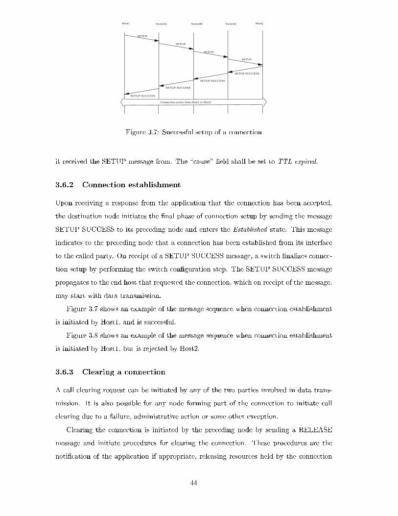
SETUP
SETUP
SETUP
SETUP
Host1 SwitchA SwitchB SwitchC Host2
SETUP SUCCESS
SETUP SUCCESS
SETUP SUCCESS
SETUP SUCCESS
Connection active from Host1 to Host2
Figure 3.7: Successful setup of a connection
it received the SETUP message from. The \cause" �eld shall be set to TTL expired.
3.6.2 Connection establishment
Upon receiving a response from the application that the connection has been accepted,
the destination node initiates the �nal phase of connection setup by sending the message
SETUP SUCCESS to its preceding node and enters the Established state. This message
indicates to the preceding node that a connection has been established from its interface
to the called party. On receipt of a SETUP SUCCESS message, a switch �nalizes connec-
tion setup by performing the switch con�guration step. The SETUP SUCCESS message
propagates to the end host that requested the connection, which on receipt of the message,
may start with data transmission.
Figure 3.7 shows an example of the message sequence when connection establishment
is initiated by Host1, and is successful.
Figure 3.8 shows an example of the message sequence when connection establishment
is initiated by Host1, but is rejected by Host2.
3.6.3 Clearing a connection
A call clearing request can be initiated by any of the two parties involved in data trans-
mission. It is also possible for any node forming part of the connection to initiate call
clearing due to a failure, administrative action or some other exception.
Clearing the connection is initiated by the preceding node by sending a RELEASE
message and initiate procedures for clearing the connection. These procedures are the
noti�cation of the application if appropriate, releasing resources held by the connection
44
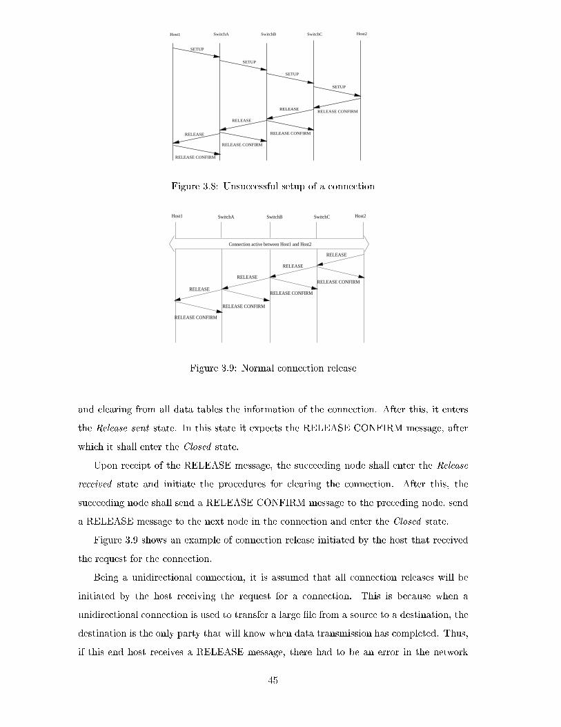
RELEASE CONFIRM
SETUP
RELEASE
RELEASE
RELEASE
SETUP
SETUP
SETUP
Host2SwitchCSwitchBSwitchAHost1
RELEASE CONFIRM
RELEASE CONFIRM
RELEASE CONFIRM
Figure 3.8: Unsuccessful setup of a connection
SwitchB SwitchC Host2SwitchAHost1
Connection active between Host1 and Host2
RELEASE
RELEASE
RELEASE CONFIRM
RELEASE
RELEASE CONFIRM
RELEASE
RELEASE CONFIRM
RELEASE CONFIRM
Figure 3.9: Normal connection release
and clearing from all data tables the information of the connection. After this, it enters
the Release sent state. In this state it expects the RELEASE CONFIRM message, after
which it shall enter the Closed state.
Upon receipt of the RELEASE message, the succeeding node shall enter the Release
received state and initiate the procedures for clearing the connection. After this, the
succeeding node shall send a RELEASE CONFIRM message to the preceding node, send
a RELEASE message to the next node in the connection and enter the Closed state.
Figure 3.9 shows an example of connection release initiated by the host that received
the request for the connection.
Being a unidirectional connection, it is assumed that all connection releases will be
initiated by the host receiving the request for a connection. This is because when a
unidirectional connection is used to transfer a large �le from a source to a destination, the
destination is the only party that will know when data transmission has completed. Thus,
if this end host receives a RELEASE message, there had to be an error in the network
45
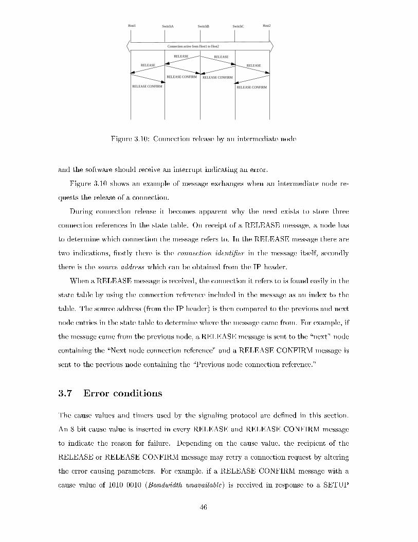
RELEASE
RELEASE
RELEASE CONFIRM
SwitchC Host2SwitchBSwitchAHost1
RELEASE CONFIRM
RELEASE CONFIRM RELEASE CONFIRM
RELEASE
RELEASE
Connection active from Host1 to Host2
Figure 3.10: Connection release by an intermediate node
and the software should receive an interrupt indicating an error.
Figure 3.10 shows an example of message exchanges when an intermediate node re-
quests the release of a connection.
During connection release it becomes apparent why the need exists to store three
connection references in the state table. On receipt of a RELEASE message, a node has
to determine which connection the message refers to. In the RELEASE message there are
two indications, �rstly there is the connection identi�er in the message itself, secondly
there is the source address which can be obtained from the IP header.
When a RELEASE message is received, the connection it refers to is found easily in the
state table by using the connection reference included in the message as an index to the
table. The source address (from the IP header) is then compared to the previous and next
node entries in the state table to determine where the message came from. For example, if
the message came from the previous node, a RELEASE message is sent to the \next" node
containing the \Next node connection reference" and a RELEASE CONFIRM message is
sent to the previous node containing the \Previous node connection reference."
3.7 Error conditions
The cause values and timers used by the signaling protocol are de�ned in this section.
An 8 bit cause value is inserted in every RELEASE and RELEASE CONFIRM message
to indicate the reason for failure. Depending on the cause value, the recipient of the
RELEASE or RELEASE CONFIRM message may retry a connection request by altering
the error causing parameters. For example, if a RELEASE CONFIRM message with a
cause value of 1010 0010 (Bandwidth unavailable) is received in response to a SETUP
46
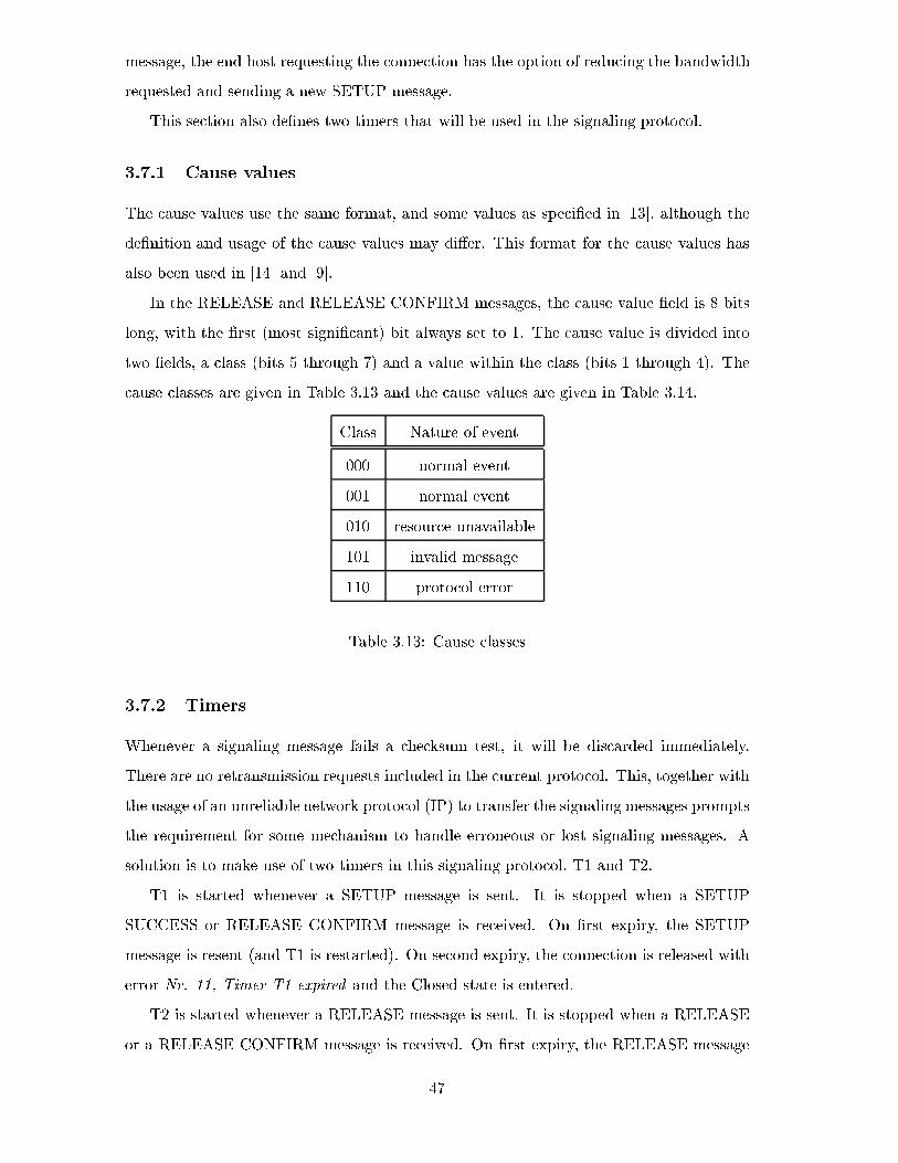
message, the end host requesting the connection has the option of reducing the bandwidth
requested and sending a new SETUP message.
This section also de�nes two timers that will be used in the signaling protocol.
3.7.1 Cause values
The cause values use the same format, and some values as speci�ed in [13], although the
de�nition and usage of the cause values may di�er. This format for the cause values has
also been used in [14] and [9].
In the RELEASE and RELEASE CONFIRM messages, the cause value �eld is 8 bits
long, with the �rst (most signi�cant) bit always set to 1. The cause value is divided into
two �elds, a class (bits 5 through 7) and a value within the class (bits 1 through 4). The
cause classes are given in Table 3.13 and the cause values are given in Table 3.14.
Class Nature of event
000 normal event
001 normal event
010 resource unavailable
101 invalid message
110 protocol error
Table 3.13: Cause classes
3.7.2 Timers
Whenever a signaling message fails a checksum test, it will be discarded immediately.
There are no retransmission requests included in the current protocol. This, together with
the usage of an unreliable network protocol (IP) to transfer the signaling messages prompts
the requirement for some mechanism to handle erroneous or lost signaling messages. A
solution is to make use of two timers in this signaling protocol, T1 and T2.
T1 is started whenever a SETUP message is sent. It is stopped when a SETUP
SUCCESS or RELEASE CONFIRM message is received. On �rst expiry, the SETUP
message is resent (and T1 is restarted). On second expiry, the connection is released with
error Nr. 11, Timer T1 expired and the Closed state is entered.
T2 is started whenever a RELEASE message is sent. It is stopped when a RELEASE
or a RELEASE CONFIRM message is received. On �rst expiry, the RELEASE message
47
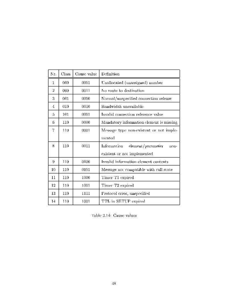
Nr. Class Cause value De�nition
1 000 0001 Unallocated (unassigned) number
2 000 0011 No route to destination
3 001 0000 Normal/unspeci�ed connection release
4 010 0010 Bandwidth unavailable
5 101 0001 Invalid connection reference value
6 110 0000 Mandatory information element is missing
7 110 0001 Message type non-existent or not imple-
mented
8 110 0011 Information element/parameter non-
existent or not implemented
9 110 0100 Invalid information element contents
10 110 0101 Message not compatible with call state
11 110 1000 Timer T1 expired
12 110 1001 Timer T2 expired
13 110 1111 Protocol error, unspeci�ed
14 110 1001 TTL in SETUP expired
Table 3.14: Cause values
48
is resent (and T2 restarted). On second expiry, the connection is released with error Nr.
12, Timer T2 expired and the Closed state is entered.
The usage of timers becomes more apparent in the case when no reply is received for
a RELEASE message. It is now possible for a connection to be released by a node, but
if its communication with its neighbour is interrupted during the connection release, the
neighbour will have resources reserved for the connection inde�nitely. The addition of
the T2 timer will only be able to solve this problem if we have a reliable network or a
reliable transport protocol for the signaling messages. Section 3.9 shall attempt to solve
this problem by introducing a reliable transport protocol.
3.7.3 Handling of error conditions
This section describes the actions to be taken when certain errors occur during connection
setup.
� Whenever the integrity check of a message (using the included checksum) fails, the
message shall be discarded.
� When a SETUP message is received with an illegal destination address, for example
127.0.0.1, a RELEASE CONFIRM message will be sent to the previous node with
cause value Nr. 1, \Unallocated (unassigned) number".
� If there is no entry in the routing table that matches the destination node, a
RELEASE CONFIRM will be sent to the previous node with cause value Nr. 2,
\No route to destination".
� A RELEASE CONFIRM message with cause value Nr. 4, \Bandwidth unavailable"
will be sent to the previous node if there is insuÆcient bandwidth available on the
outgoing interface connected to the next hop.
� If a RELEASE message is received indicating a connection reference value which
is not recognized as an active connection, or a connection setup in progress, a
RELEASE CONFIRM message with cause value Nr. 5, \Invalid connection ref-
erence value" is sent in reply. Remain in the Closed state.
� If a SETUP SUCCESS message is received indicating a connection reference value
which is not recognized as a connection setup in progress, a RELEASE CONFIRM
49
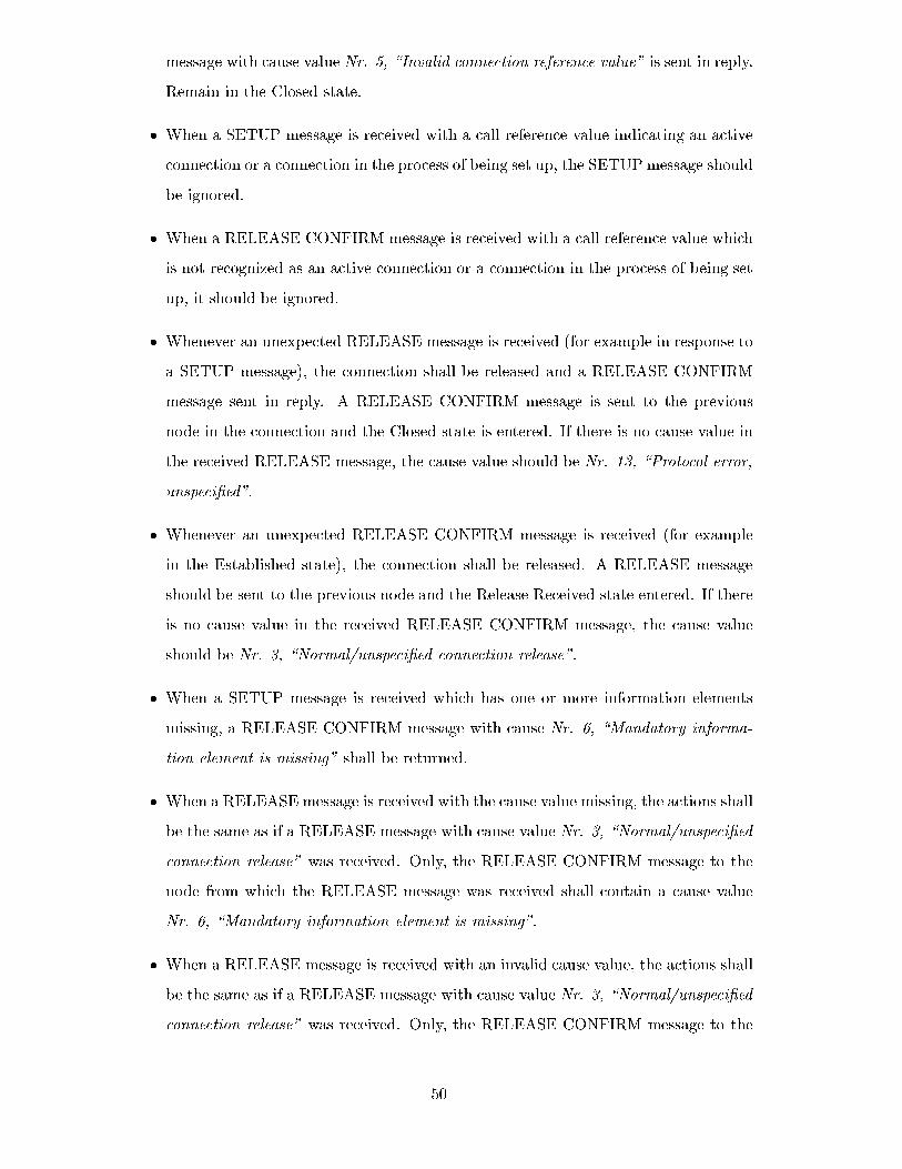
message with cause value Nr. 5, \Invalid connection reference value" is sent in reply.
Remain in the Closed state.
� When a SETUP message is received with a call reference value indicating an active
connection or a connection in the process of being set up, the SETUP message should
be ignored.
� When a RELEASE CONFIRM message is received with a call reference value which
is not recognized as an active connection or a connection in the process of being set
up, it should be ignored.
� Whenever an unexpected RELEASE message is received (for example in response to
a SETUP message), the connection shall be released and a RELEASE CONFIRM
message sent in reply. A RELEASE CONFIRM message is sent to the previous
node in the connection and the Closed state is entered. If there is no cause value in
the received RELEASE message, the cause value should be Nr. 13, \Protocol error,
unspeci�ed".
� Whenever an unexpected RELEASE CONFIRM message is received (for example
in the Established state), the connection shall be released. A RELEASE message
should be sent to the previous node and the Release Received state entered. If there
is no cause value in the received RELEASE CONFIRM message, the cause value
should be Nr. 3, \Normal/unspeci�ed connection release".
� When a SETUP message is received which has one or more information elements
missing, a RELEASE CONFIRM message with cause Nr. 6, \Mandatory informa-
tion element is missing" shall be returned.
� When a RELEASE message is received with the cause value missing, the actions shall
be the same as if a RELEASE message with cause value Nr. 3, \Normal/unspeci�ed
connection release" was received. Only, the RELEASE CONFIRM message to the
node from which the RELEASE message was received shall contain a cause value
Nr. 6, \Mandatory information element is missing".
� When a RELEASE message is received with an invalid cause value, the actions shall
be the same as if a RELEASE message with cause value Nr. 3, \Normal/unspeci�ed
connection release" was received. Only, the RELEASE CONFIRM message to the
50
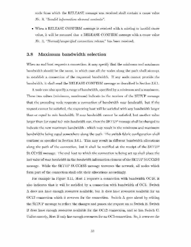
node from which the RELEASE message was received shall contain a cause value
Nr. 9, \Invalid information element contents".
� When a RELEASE CONFIRM message is received with a missing or invalid cause
value, it will be assumed that a RELEASE CONFIRM message with a cause value
Nr. 3, \Normal/unspeci�ed connection release" has been received.
3.8 Maximum bandwidth selection
When an end host requests a connection, it may specify that the minimum and maximum
bandwidth should be the same, in which case all the nodes along the path shall attempt
to establish a connection of the requested bandwidth. If any node cannot provide the
bandwidth, it shall send the RELEASE CONFIRM message as described in Section 3.6.1.
A node can also specify a range of bandwidth, speci�ed by a minimum and a maximum.
These two values (minimum, maximum) indicate to the receiver of the SETUP message
that the preceding node requests a connection of bandwidth max bandwidth, but if the
request cannot be satis�ed, the requesting host will be satis�ed with any bandwidth larger
than or equal to min bandwidth. If max bandwidth cannot be satis�ed, but another value
larger than (or equal to) min bandwidth can, then the SETUP message shall be changed to
indicate the new maximum bandwidth - which may result in the minimum and maximum
bandwidths being equal somewhere along the path. The switch fabric con�guration shall
continue as speci�ed in Section 3.6.1. This may result in di�erent bandwidth allocations
along the path of the connection, but it shall be recti�ed at the receipt of the SETUP
SUCCESS message. The end host to which the connection is being set up shall place the
last value ofmax bandwidth in the bandwidth information element of the SETUP SUCCESS
message. While the SETUP SUCCESS message traverses the network, all nodes which
form part of the connection shall edit their allocations accordingly.
For example in Figure 3.11, Host 1 requests a connection with bandwidth OC48, it
also indicates that it will be satis�ed by a connection with bandwidth of OC3. Switch
A does not have enough resources available, but it does have resources available for an
OC12 connection which it reserves for the connection. Switch A goes ahead by editing
the SETUP message to re ect the changes and passes the request on to Switch B. Switch
B does have enough resources available for the OC12 connection, and so has Switch C.
Unfortunately, Host B only has enough resources for an OC3 connection. So, it reserves the
51
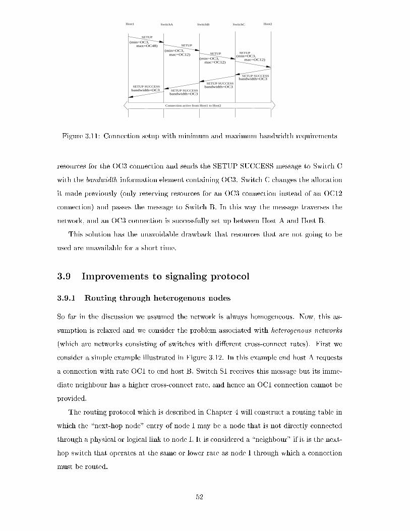
SETUP
SETUP
SETUP
Host1 SwitchA SwitchB SwitchC Host2
SETUP SUCCESS
SETUP SUCCESS
SETUP SUCCESS
SETUP SUCCESS
(min=OC3,
SETUP(min=OC3,
(min=OC3,(min=OC3,mac=OC12)
mac=OC12)mac=OC12)
bandwidth=OC3
bandwidth=OC3
bandwidth=OC3bandwidth=OC3
Connection active from Host1 to Host2
max=OC48)
Figure 3.11: Connection setup with minimum and maximum bandwidth requirements
resources for the OC3 connection and sends the SETUP SUCCESS message to Switch C
with the bandwidth information element containing OC3. Switch C changes the allocation
it made previously (only reserving resources for an OC3 connection instead of an OC12
connection) and passes the message to Switch B. In this way the message traverses the
network, and an OC3 connection is successfully set up between Host A and Host B.
This solution has the unavoidable drawback that resources that are not going to be
used are unavailable for a short time.
3.9 Improvements to signaling protocol
3.9.1 Routing through heterogenous nodes
So far in the discussion we assumed the network is always homogeneous. Now, this as-
sumption is relaxed and we consider the problem associated with heterogenous networks
(which are networks consisting of switches with di�erent cross-connect rates). First we
consider a simple example illustrated in Figure 3.12. In this example end host A requests
a connection with rate OC1 to end host B. Switch S1 receives this message but its imme-
diate neighbour has a higher cross-connect rate, and hence an OC1 connection cannot be
provided.
The routing protocol which is described in Chapter 4 will construct a routing table in
which the \next-hop node" entry of node I may be a node that is not directly connected
through a physical or logical link to node I. It is considered a \neighbour" if it is the next-
hop switch that operates at the same or lower rate as node I through which a connection
must be routed.
52
S1 S1
S2S2
S3 S3
OC1 OC1 OC1 OC1
OC12OC12
Step 1: Set up an OC12 through neighbor S2 Step 2: Set up an OC1 on the new logical OC12 link
Setup(OC1)
Setup(OC12)
Setup(OC1)Setup(OC1)
Setup(OC1)
Setup(OC12)
SetupSuccess
SetupSuccess
between S1 and S3
EHA
EHB
EH EHA B
Figure 3.12: Connection setup in heterogenous network
Connection setup in a heterogenous network can now be explained as follows. If the
\next-hop node" entry in the routing table indicates a node that is not an immediate
neighbour of node I (physically or logically) as determined by examining the connectivity
table, the routing table is queried again to locate which immediate neighbour should
be used to reach the \next-hop node" of node I. Assume that node J is the immediate
neighbour and node K is the \next-hop node". Node I must determine the cross-connect
rate of node J and request a connection setup at this rate between itself and node K. Once
this is complete, the setting up of the lower rate connection can proceed over the newly
created logical link between nodes I and K.
In the example of Figure 3.12, the routing table of switch S1 will look as follows. For
data rate OC1 and destination B the \next-hop node" shall be given as S3. According to
the information in the connectivity table (Table 3.5) S3 is not a neighbour of S1. So, it
has to search the routing table again to look for the entry where S3 is a destination. The
lowest data rate at which there is an entry for S3 shall be used as the requested rate when
a connection is set up between itself and S3. Once this connection is established, nodes
S1 and S3 become immediate neighbours on this newly created logical link. Switch S1 can
then send the OC1 Setup request to switch S3 for further routing as shown in Step 2 of
Figure 3.12.
Another example is given in Figure 3.13. In this example end host A starts by sending
a setup request to switch S1 for a connection of rate OC12 to end host B. Switches S1, S2
and S3 can all handle the connection requirements due to their cross-connect rates being
smaller or equal to the requested rate. We shall follow the progress of the connection setup
from switch S3.
Switch S3 receives the setup request for an OC12 connection, to pass the connection
setup request on to the next hop it queries the routing table. The routing table has an
53
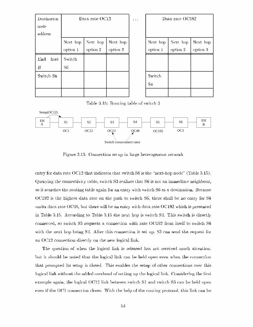
Destination
node
address
Data rate OC12 : : : Data rate OC192
Next hop
option 1
Next hop
option 2
Next hop
option 3
Next hop
option 1
Next hop
option 2
Next hop
option 3
End host
B
Switch
S6
Switch S6 Switch
S4
Table 3.15: Routing table of switch 3
OC12OC1 OC12 OC48 OC192 OC3
S1 S2 S3 S4 S5 S6A BEH EH
Switch crossconnect rates
Setup(OC12)
Figure 3.13: Connection setup in large heterogenous network
entry for data rate OC12 that indicates that switch S6 is the \next-hop node" (Table 3.15).
Querying the connectivity table, switch S3 realizes that S6 is not an immediate neighbour,
so it searches the routing table again for an entry with switch S6 as a destination. Because
OC192 is the highest data rate on the path to switch S6, there shall be no entry for S6
under data rate OC48, but there will be an entry with data rate OC192 which is presented
in Table 3.15. According to Table 3.15 the next hop is switch S4. This switch is directly
connected, so switch S3 requests a connection with rate OC192 from itself to switch S6
with the next hop being S4. After this connection is set up, S3 can send the request for
an OC12 connection directly on the new logical link.
The question of when the logical link is released has not received much attention,
but it should be noted that the logical link can be held open even when the connection
that prompted its setup is closed. This enables the setup of other connections over this
logical link without the added overhead of setting up the logical link. Considering the �rst
example again, the logical OC12 link between switch S1 and switch S3 can be held open
even if the OC1 connection closes. With the help of the routing protocol, this link can be
54
advertised, and new OC1 connections can be set up over it. Once the last OC1 connection
closes, a timer can be started, if no new requests for OC1 connections are received before
the timer's expiration, the logical link can be closed.
Note that when a connection passes through a switch with a lower crossconnect rate,
for example by realizing an OC12 connection as 12 OC1 connections, some mechanism
of multiplexing/demultiplexing is required. These actions have been assumed to occur
transparently because of the synchronous nature of the SONET network.
3.9.2 Transport of signaling messages
Transporting the signaling messages over the IP network has already introduced two im-
portant limitations. Firstly, using IP without TCP implies unreliable transmission. The
network does not provide any guarantee that the signaling message will reach its destina-
tion, there is no indication if the signaling message has reached its destination and if the
message reaches the destination, there is no guarantee the data is intact. As described
in Section 3.7.2, the unreliable nature of the network can cause some switches to waste
valuable resources. The second limitation is security. Although this is not the focus of
this research, the lack of authentication mechanisms, together with the use of a public
network for the transport of the signaling messages might introduce some security risks,
for example denial of service attacks, to the circuit switched network. The use of a private
IP network just to transport signaling messages is wasteful of resources.
The IETF Signaling Transport working group is currently working on the Stream Con-
trol Transmission Protocol (SCTP) [22]. SCTP started out as a transport protocol for
PSTN signaling messages over the IP network, but the capabilities of this protocol will
solve the problems introduced when only IP is used to transfer the signaling messages.
SCTP provides acknowledged error-free non-duplicated transfer of user data and is re-
sistant to ooding and masquerade attacks [22]. However, with our goal for hardware
implementation, it still needs to be determined if SCTP or TCP can be implemented in
hardware.
Another option is to carry the signaling messages using SONET. Inside a SONET frame
there are three section overhead bytes (named D1, D2 and D3) and eight line overhead
bytes (named D4 to D12). These bytes are termed the section data communications
channel (DCC) and line data communication channel (DCC) respectively and are used for
operations, administration, maintenance and provisioning (OAM&P). Carrying signaling
55
messages on one of these point-to-point DCC channels will eliminate the need for an IP
network.
3.10 Conclusion
Signaling protocols in current TDM networks only provide low-bandwidth (DS0) circuits
on demand to one application (telephony). This chapter describes a new hardware imple-
mentable signaling protocol that is able to provide high-bandwidth on-demand circuits for
applications such as bulk data transfers. The signaling protocol presented in this chapter
requires a supporting routing protocol. The routing protocol that will be presented in
Chapter 4 is responsible for the creation of the routing table entries that are required by
the signaling protocol.
56
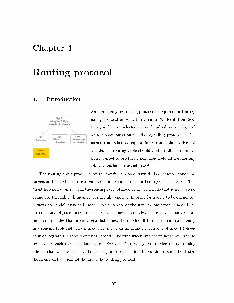
Chapter 4
Routing protocol
4.1 Introduction
Chapter 2Analyzing file transfer delays in
circuit-switched and TCP/IP networks.
Chapter 6Further work:
Transport layer
Chapter 3
Signaling protocol
Chapter 5Scheduling calls with known holding times
Chapter 4
Routing protocol
An accompanying routing protocol is required for the sig-
naling protocol presented in Chapter 3. Recall from Sec-
tion 3.4 that we selected to use hop-by-hop routing and
route precomputation for the signaling protocol. This
means that when a request for a connection arrives at
a node, the routing table should contain all the informa-
tion required to produce a next-hop node address for any
address reachable through itself.
The routing table produced by the routing protocol should also contain enough in-
formation to be able to accommodate connection setup in a heterogenous network. The
\next-hop node" entry, J, in the routing table of node I may be a node that is not directly
connected through a physical or logical link to node I. In order for node J to be considered
a \next-hop node" by node I, node J must operate at the same or lower rate as node I. As
a result, on a physical path from node I to the next-hop node J there may be one or more
intervening nodes that are not regarded as next-hop nodes. If the \next-hop node" entry
in a routing table indicates a node that is not an immediate neighbour of node I (physi-
cally or logically), a second entry is needed indicating which immediate neighbour should
be used to reach the \next-hop node". Section 4.2 starts by introducing the addressing
scheme that will be used by the routing protocol, Section 4.3 continues with the design
decisions, and Section 4.4 describes the routing protocol.
57
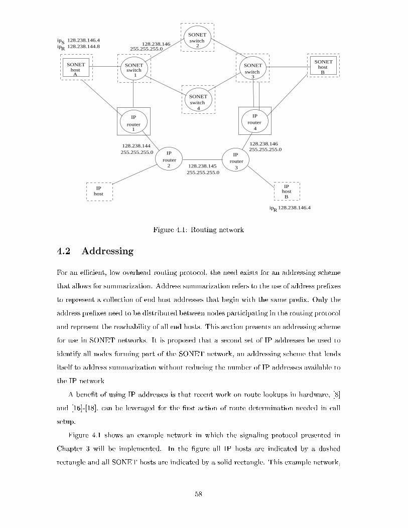
IP IP
IP IP
SONETswitch
SONETswitch
SONETswitch
IP
SONEThost
SONETswitch
router router
router router
host
128.238.145
128.238.144 128.238.146
1
2
3
4
1
2 3
4
128.238.146
A
ip 128.238.146.4SRip 128.238.144.8
255.255.255.0
255.255.255.0255.255.255.0
255.255.255.0
IPhostB
ip 128.238.146.4R
SONEThost
B
Figure 4.1: Routing network
4.2 Addressing
For an eÆcient, low overhead routing protocol, the need exists for an addressing scheme
that allows for summarization. Address summarization refers to the use of address pre�xes
to represent a collection of end host addresses that begin with the same pre�x. Only the
address pre�xes need to be distributed between nodes participating in the routing protocol
and represent the reachability of all end hosts. This section presents an addressing scheme
for use in SONET networks. It is proposed that a second set of IP addresses be used to
identify all nodes forming part of the SONET network, an addressing scheme that lends
itself to address summarization without reducing the number of IP addresses available to
the IP network
A bene�t of using IP addresses is that recent work on route lookups in hardware, [8]
and [16]-[18], can be leveraged for the �rst action of route determination needed in call
setup.
Figure 4.1 shows an example network in which the signaling protocol presented in
Chapter 3 will be implemented. In the �gure all IP hosts are indicated by a dashed
rectangle and all SONET hosts are indicated by a solid rectangle. This example network,
58
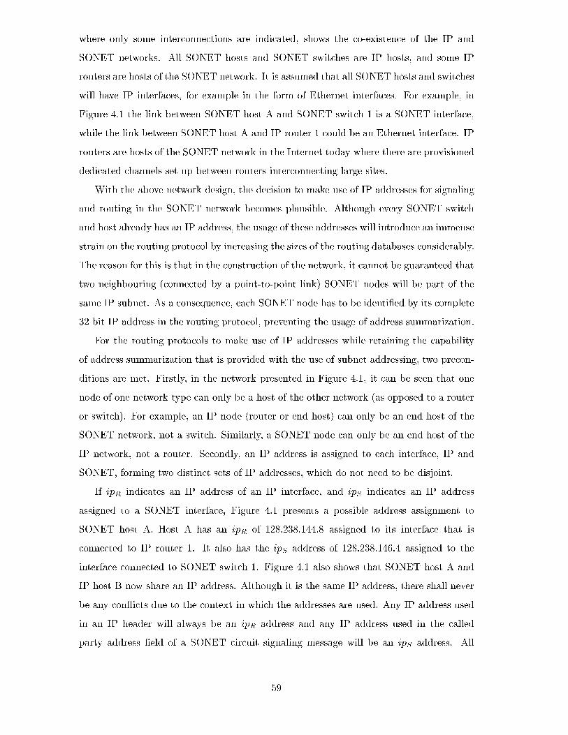
where only some interconnections are indicated, shows the co-existence of the IP and
SONET networks. All SONET hosts and SONET switches are IP hosts, and some IP
routers are hosts of the SONET network. It is assumed that all SONET hosts and switches
will have IP interfaces, for example in the form of Ethernet interfaces. For example, in
Figure 4.1 the link between SONET host A and SONET switch 1 is a SONET interface,
while the link between SONET host A and IP router 1 could be an Ethernet interface. IP
routers are hosts of the SONET network in the Internet today where there are provisioned
dedicated channels set up between routers interconnecting large sites.
With the above network design, the decision to make use of IP addresses for signaling
and routing in the SONET network becomes plausible. Although every SONET switch
and host already has an IP address, the usage of these addresses will introduce an immense
strain on the routing protocol by increasing the sizes of the routing databases considerably.
The reason for this is that in the construction of the network, it cannot be guaranteed that
two neighbouring (connected by a point-to-point link) SONET nodes will be part of the
same IP subnet. As a consequence, each SONET node has to be identi�ed by its complete
32 bit IP address in the routing protocol, preventing the usage of address summarization.
For the routing protocols to make use of IP addresses while retaining the capability
of address summarization that is provided with the use of subnet addressing, two precon-
ditions are met. Firstly, in the network presented in Figure 4.1, it can be seen that one
node of one network type can only be a host of the other network (as opposed to a router
or switch). For example, an IP node (router or end host) can only be an end host of the
SONET network, not a switch. Similarly, a SONET node can only be an end host of the
IP network, not a router. Secondly, an IP address is assigned to each interface, IP and
SONET, forming two distinct sets of IP addresses, which do not need to be disjoint.
If ipR indicates an IP address of an IP interface, and ipS indicates an IP address
assigned to a SONET interface, Figure 4.1 presents a possible address assignment to
SONET host A. Host A has an ipR of 128.238.144.8 assigned to its interface that is
connected to IP router 1. It also has the ipS address of 128.238.146.4 assigned to the
interface connected to SONET switch 1. Figure 4.1 also shows that SONET host A and
IP host B now share an IP address. Although it is the same IP address, there shall never
be any con icts due to the context in which the addresses are used. Any IP address used
in an IP header will always be an ipR address and any IP address used in the called
party address �eld of a SONET circuit signaling message will be an ipS address. All
59
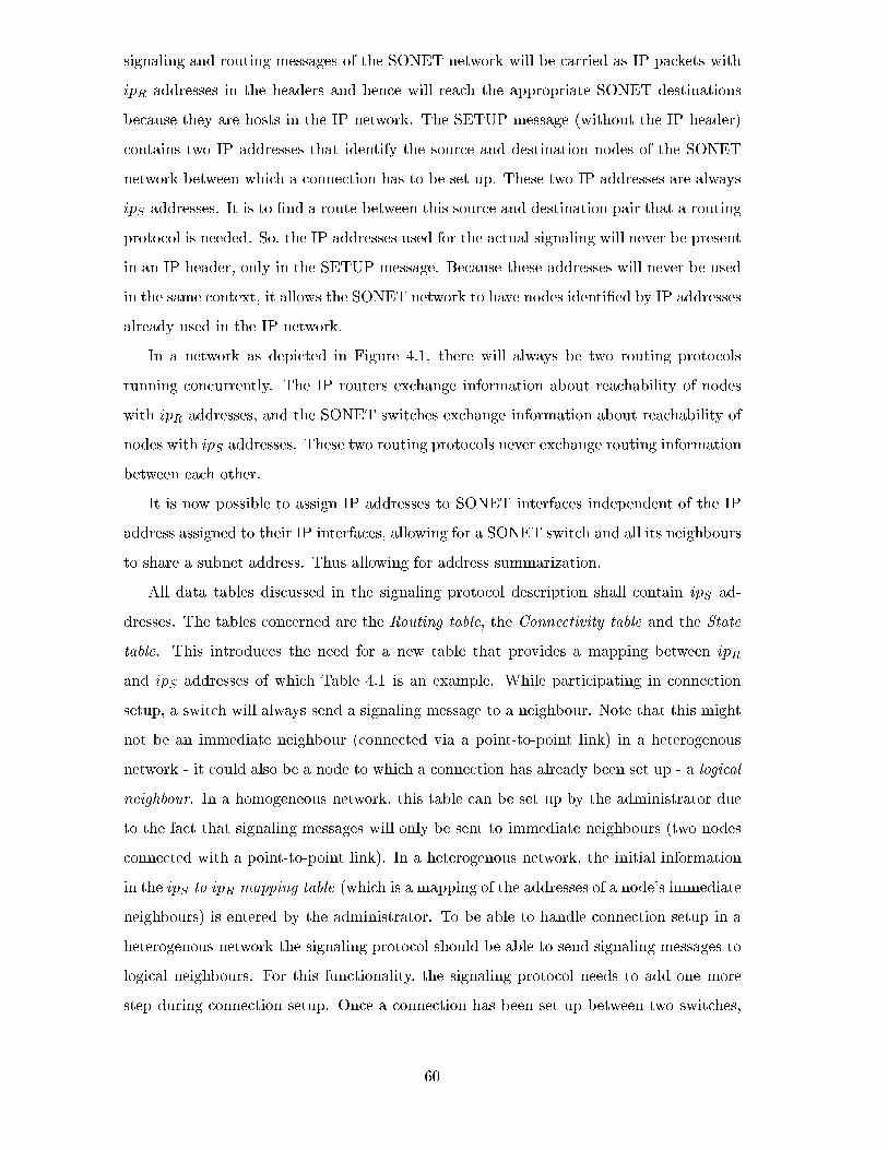
signaling and routing messages of the SONET network will be carried as IP packets with
ipR addresses in the headers and hence will reach the appropriate SONET destinations
because they are hosts in the IP network. The SETUP message (without the IP header)
contains two IP addresses that identify the source and destination nodes of the SONET
network between which a connection has to be set up. These two IP addresses are always
ipS addresses. It is to �nd a route between this source and destination pair that a routing
protocol is needed. So, the IP addresses used for the actual signaling will never be present
in an IP header, only in the SETUP message. Because these addresses will never be used
in the same context, it allows the SONET network to have nodes identi�ed by IP addresses
already used in the IP network.
In a network as depicted in Figure 4.1, there will always be two routing protocols
running concurrently. The IP routers exchange information about reachability of nodes
with ipR addresses, and the SONET switches exchange information about reachability of
nodes with ipS addresses. These two routing protocols never exchange routing information
between each other.
It is now possible to assign IP addresses to SONET interfaces independent of the IP
address assigned to their IP interfaces, allowing for a SONET switch and all its neighbours
to share a subnet address. Thus allowing for address summarization.
All data tables discussed in the signaling protocol description shall contain ipS ad-
dresses. The tables concerned are the Routing table, the Connectivity table and the State
table. This introduces the need for a new table that provides a mapping between ipR
and ipS addresses of which Table 4.1 is an example. While participating in connection
setup, a switch will always send a signaling message to a neighbour. Note that this might
not be an immediate neighbour (connected via a point-to-point link) in a heterogenous
network - it could also be a node to which a connection has already been set up - a logical
neighbour. In a homogeneous network, this table can be set up by the administrator due
to the fact that signaling messages will only be sent to immediate neighbours (two nodes
connected with a point-to-point link). In a heterogenous network, the initial information
in the ipS to ipR mapping table (which is a mapping of the addresses of a node's immediate
neighbours) is entered by the administrator. To be able to handle connection setup in a
heterogenous network the signaling protocol should be able to send signaling messages to
logical neighbours. For this functionality, the signaling protocol needs to add one more
step during connection setup. Once a connection has been set up between two switches,
60
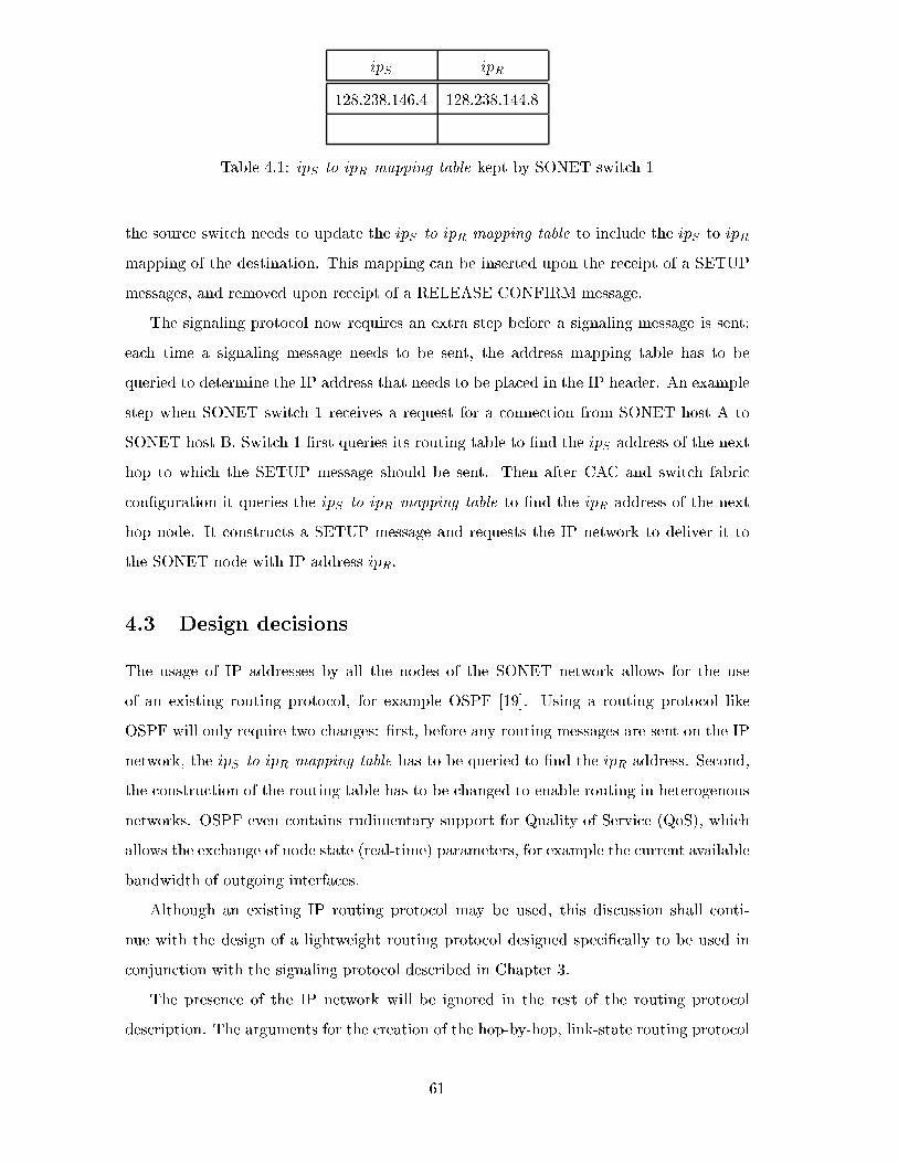
ipS ipR
128.238.146.4 128.238.144.8
Table 4.1: ipS to ipR mapping table kept by SONET switch 1
the source switch needs to update the ipS to ipR mapping table to include the ipS to ipR
mapping of the destination. This mapping can be inserted upon the receipt of a SETUP
messages, and removed upon receipt of a RELEASE CONFIRM message.
The signaling protocol now requires an extra step before a signaling message is sent:
each time a signaling message needs to be sent, the address mapping table has to be
queried to determine the IP address that needs to be placed in the IP header. An example
step when SONET switch 1 receives a request for a connection from SONET host A to
SONET host B. Switch 1 �rst queries its routing table to �nd the ipS address of the next
hop to which the SETUP message should be sent. Then after CAC and switch fabric
con�guration it queries the ipS to ipR mapping table to �nd the ipR address of the next
hop node. It constructs a SETUP message and requests the IP network to deliver it to
the SONET node with IP address ipR.
4.3 Design decisions
The usage of IP addresses by all the nodes of the SONET network allows for the use
of an existing routing protocol, for example OSPF [19]. Using a routing protocol like
OSPF will only require two changes: �rst, before any routing messages are sent on the IP
network, the ipS to ipR mapping table has to be queried to �nd the ipR address. Second,
the construction of the routing table has to be changed to enable routing in heterogenous
networks. OSPF even contains rudimentary support for Quality of Service (QoS), which
allows the exchange of node state (real-time) parameters, for example the current available
bandwidth of outgoing interfaces.
Although an existing IP routing protocol may be used, this discussion shall conti-
nue with the design of a lightweight routing protocol designed speci�cally to be used in
conjunction with the signaling protocol described in Chapter 3.
The presence of the IP network will be ignored in the rest of the routing protocol
description. The arguments for the creation of the hop-by-hop, link-state routing protocol
61
that creates a routing table by constructing a shortest path tree is described next.
Section 3.4 brie y mentioned the decision that the options of route precomputa-
tion and hop-by-hop routing (as opposed to source routing) will be used in the routing
protocol. Using SONET it is possible to make full use of route precomputation due to the
granularity of the multiplexing rates. As depicted in Table 3.3, next-hop entries are only
kept for the SONET rates of OC1, OC3, OC12, OC48 and OC192. This simpli�es the
connection setup procedure in that the route determination step is just a table lookup.
There are two reasons for the decision of hop-by-hop routing. Firstly, by using hop-by-hop
routing the parsing of the SETUP message is simpli�ed at each hop allowing for hardware
implementation. Secondly, when source routing is used it is possible that conditions change
as connection setup proceeds from a given source node toward a destination, and by the
time the setup request reaches an intermediate node, the selected source route is no longer
available, in which case crankbacks are needed. Crankbacks require the management of
more state information, which leads to increased hardware complexity.
The routing protocol should be executed in parallel by all the SONET switches, without
segmenting the network. This allows all the nodes to have an identical copy of the routing
database. The reason that the current routing protocol proposal requires a at network
structure (no segmentation) is for simplicity. The moment a network is segmented, the
di�erent \areas" can receive summarized information regarding the real time parameters
in the other areas. Because the information is summarized, some mechanism similar to
Generic CAC (GCAC) from PNNI needs to be applied to a connection request before
it is passed on to the next hop (together with the CAC performed by the node itself).
GCAC allows a node to predict the outcome of the actual CAC performed at another
switching system given that node's advertised additive link metrics. Performing GCAC
will add complexity to the signaling protocol, and will heighten the risk that the real CAC
performed by a switch further along the path (possibly in another area) may fail. This
failure will introduce crankback. A at network structure avoids this problem.
Routing databases tend to be very large. Using a routing protocol to distribute real
time parameters, for example the available bandwidth of an interface, requires the pro-
tocol to always have up to date information in the database and to respond quickly to
any changes in the database. A distance-vector routing protocol such as RIP [20] would
be ineÆcient when used in large networks (large routing databases). A distance-vector
algorithm, such as the Bellman-Ford algorithm used by RIP, does not perform well when
62
there is a large database and a topology change occurs or a change in a node's real time
parameters occurs. This is because a change in the network results in a convergence period
which might not be fast enough for the routing protocol to be usable.
In distance-vector algorithms, each node keeps a table with an entry for every possible
destination reachable though itself. The entry indicates the distance to the destination
and the next-hop node to the destination. The distances are continually compared and
updated as routing update messages are received by a node. Once a topology change
occurs (for example a link goes down), and the changes to the distances are distributes
through the network, the routing tables will not immediately see the change because some
nodes will still consider the link as active and re ect that in their advertisements. This is
the cause of the convergence period that is the time for a node's routing table to re ect
the correct distance values to the a�ected destinations.
It is thus proposed to make use of a link state routing algorithm. In this algorithm
each node has an identical routing database containing the identity (address) and con-
nectivity of each node in the network from which a routing table is constructed. The
routing table entries are calculated by constructing a shortest path tree. By using a link
state routing algorithm, any changes in the network topology or real-time parameters of
nodes in the network will be received by all the nodes executing the routing protocol very
quickly, thus enabling all the nodes to have the most up to date information regarding
topology and real time parameters. With this information the routing protocol is able to
make more accurate routing decisions than a distance-vector routing protocol.
Information distributed by the switching systems participating in the routing protocol
should contain enough detail about their respective identity (reachability) and capabil-
ity. Information concerning individual end hosts' capability (for example an end host's
interface rate) cannot be distributed due to the usage of address summarization. This
information (identity and capability) can also be described as nodal information and in
this implementation it describes the node's address (the ipS address) and the cross con-
nect rate of the switching system. Together with the nodal information, the protocol also
distributes topological information, which is information regarding the links between the
switching systems. The topological information is a non-negative cost assigned to an out-
going interface based upon the amount of available bandwidth at the interface: the higher
the available bandwidth of an interface, the lower the cost value. A lower cost value thus
indicates a higher probability for this interface to be chosen.
63
At initialization, a node advertises that it has an available bandwidth equal to the
interface rate (resulting in a low cost value). It is proposed that the distribution of
subsequent topological information be based upon threshold computations. That is the
node participating in the routing protocol should not send a routing update message every
time a connection is admitted or released. Only when the available bandwidth reaches a
certain threshold should it send out a routing update message containing a higher cost
value to indicate a change in its available bandwidth.
As with the signaling protocol, the routing protocol also makes use of the IP network to
distribute routing database updates. Considering the delay involved in the connectionless
network, the usage real-time parameters might introduce some connection setup failures.
For example, if node I passes a connection request to node I+1 based on the information
in its routing database that states that node I+1 does have enough bandwidth available,
and at the same time , node I+1 sends out a routing update message that it does not have
enough bandwidth available - the connection request will fail. For this reason multiple
next hop entries are kept in the routing table. If the connection request fails, the setup
request is reconstructed and sent to the second (or third) option for a next hop node.
4.4 Protocol description
The routing protocol will be described through its four components. All the switching
systems in the network have an identical routing database that describes the nodal and
topological information of each node in the network. This database allows each node to
construct a directed graph representing the network. From this directed graph, each
switching system constructs the shortest path tree with itself as the root, and using
this tree it is now possible to compute the routing table entries.
An example network is shown in Figure 4.2. This example, and all the examples in
this chapter will refer to the switching systems by their names (SwitchA, SwitchB, etc.).
Note that this representation is used to simplify the explanations, an implementation
would use the IP (ipS) addresses. Each directed line indicates a unidirectional connection
between two switching systems. A cost is associated with each outgoing interface. The
cross connect rates are also depicted because these values play an important role in the
construction of the routing table.
64

10
6
7
1
2
3
45
8
9
6
Switch A
Switch B
Switch D
Switch C
Switch E
OC3
OC3
OC1
OC1
OC1
Figure 4.2: Example network con�guration for routing protocol
Next hop node Interface number Total bandwidth Available bandwidth Cost
Table 4.2: Available bandwidth table including cost
4.4.1 Routing database and directed graph
For this routing protocol, each switching system needs to know to which other nodes it is
directly connected. This information is currently stored in the Connectivity and Available
bandwidth tables used by the signaling protocol. All connections will be unidirectional,
so we are only interested in the succeeding, directly connected nodes. This information
is stored in the Available bandwidth table. The cost associated with an interface is pro-
grammed into the Available bandwidth table, Table 3.4, of which Table 4.2 is a copy. The
cost is a decreasing function of the available bandwidth of an interface - the higher the
available bandwidth, the lower the cost.
For each node n (including itself) in the network, the routing database of each switching
system in the network contains information indicated by the �rst column of Table 4.3.
� Node id refers to the ipS address of node n.
� The sequence number characterizes the last routing update concerning node n.
65
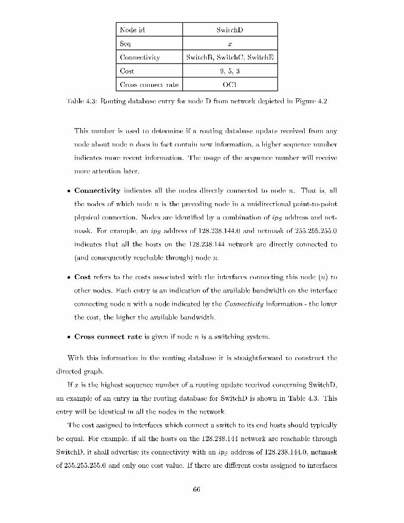
Node id SwitchD
Seq x
Connectivity SwitchB, SwitchC, SwitchE
Cost 9, 5, 3
Cross connect rate OC1
Table 4.3: Routing database entry for node D from network depicted in Figure 4.2
This number is used to determine if a routing database update received from any
node about node n does in fact contain new information, a higher sequence number
indicates more recent information. The usage of the sequence number will receive
more attention later.
� Connectivity indicates all the nodes directly connected to node n. That is, all
the nodes of which node n is the preceding node in a unidirectional point-to-point
physical connection. Nodes are identi�ed by a combination of ipS address and net-
mask. For example, an ipS address of 128.238.144.0 and netmask of 255.255.255.0
indicates that all the hosts on the 128.238.144 network are directly connected to
(and consequently reachable through) node n.
� Cost refers to the costs associated with the interfaces connecting this node (n) to
other nodes. Each entry is an indication of the available bandwidth on the interface
connecting node n with a node indicated by the Connectivity information - the lower
the cost, the higher the available bandwidth.
� Cross connect rate is given if node n is a switching system.
With this information in the routing database it is straightforward to construct the
directed graph.
If x is the highest sequence number of a routing update received concerning SwitchD,
an example of an entry in the routing database for SwitchD is shown in Table 4.3. This
entry will be identical in all the nodes in the network.
The cost assigned to interfaces which connect a switch to its end hosts should typically
be equal. For example, if all the hosts on the 128.238.144 network are reachable through
SwitchD, it shall advertise its connectivity with an ipS address of 128.238.144.0, netmask
of 255.255.255.0 and only one cost value. If there are di�erent costs assigned to interfaces
66
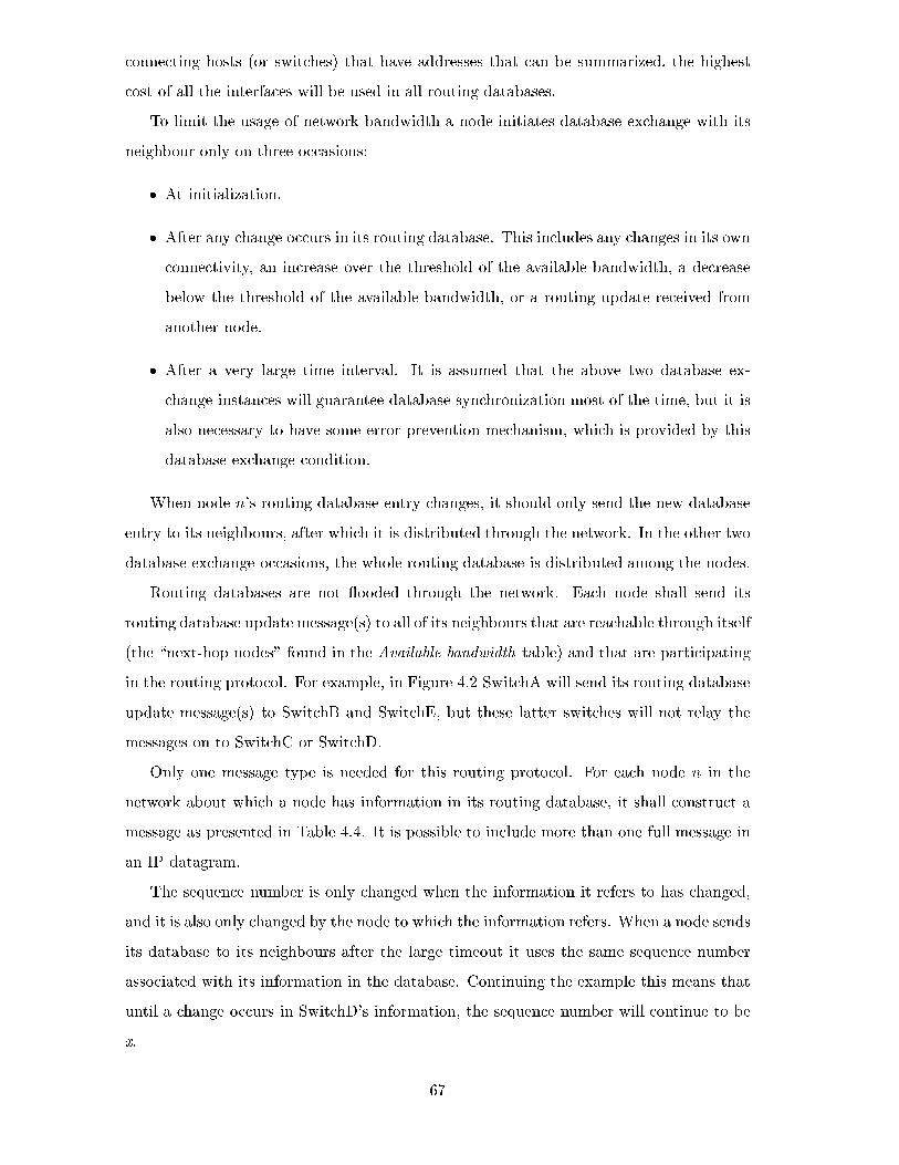
connecting hosts (or switches) that have addresses that can be summarized, the highest
cost of all the interfaces will be used in all routing databases.
To limit the usage of network bandwidth a node initiates database exchange with its
neighbour only on three occasions:
� At initialization.
� After any change occurs in its routing database. This includes any changes in its own
connectivity, an increase over the threshold of the available bandwidth, a decrease
below the threshold of the available bandwidth, or a routing update received from
another node.
� After a very large time interval. It is assumed that the above two database ex-
change instances will guarantee database synchronization most of the time, but it is
also necessary to have some error prevention mechanism, which is provided by this
database exchange condition.
When node n's routing database entry changes, it should only send the new database
entry to its neighbours, after which it is distributed through the network. In the other two
database exchange occasions, the whole routing database is distributed among the nodes.
Routing databases are not ooded through the network. Each node shall send its
routing database update message(s) to all of its neighbours that are reachable through itself
(the \next-hop nodes" found in the Available bandwidth table) and that are participating
in the routing protocol. For example, in Figure 4.2 SwitchA will send its routing database
update message(s) to SwitchB and SwitchE, but these latter switches will not relay the
messages on to SwitchC or SwitchD.
Only one message type is needed for this routing protocol. For each node n in the
network about which a node has information in its routing database, it shall construct a
message as presented in Table 4.4. It is possible to include more than one full message in
an IP datagram.
The sequence number is only changed when the information it refers to has changed,
and it is also only changed by the node to which the information refers. When a node sends
its database to its neighbours after the large timeout it uses the same sequence number
associated with its information in the database. Continuing the example this means that
until a change occurs in SwitchD's information, the sequence number will continue to be
x.
67
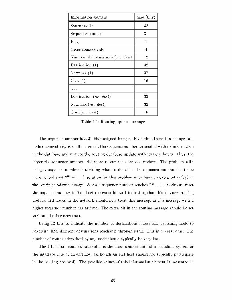
Information element Size (bits)
Source node 32
Sequence number 31
Flag 1
Cross connect rate 4
Number of destinations (nr. dest) 12
Destination (1) 32
Netmask (1) 32
Cost (1) 16
: : :
Destination (nr. dest) 32
Netmask (nr. dest) 32
Cost (nr. dest) 16
Table 4.4: Routing update message
The sequence number is a 31 bit unsigned integer. Each time there is a change in a
node's connectivity it shall increment the sequence number associated with its information
in the database and initiate the routing database update with its neighbours. Thus, the
larger the sequence number, the more recent the database update. The problem with
using a sequence number is deciding what to do when the sequence number has to be
incremented past 231 � 1. A solution for this problem is to have an extra bit (Flag) in
the routing update message. When a sequence number reaches 231 � 1 a node can reset
the sequence number to 0 and set the extra bit to 1 indicating that this is a new routing
update. All nodes in the network should now treat this message as if a message with a
higher sequence number has arrived. The extra bit in the routing message should be set
to 0 on all other occasions.
Using 12 bits to indicate the number of destinations allows any switching node to
advertise 4095 di�erent destinations reachable through itself. This is a worst case. The
number of routes advertised by any node should typically be very low.
The 4 bit cross connect rate value is the cross connect rate of a switching system or
the interface rate of an end host (although an end host should not typically participate
in the routing protocol). The possible values of this information element is presented in
68
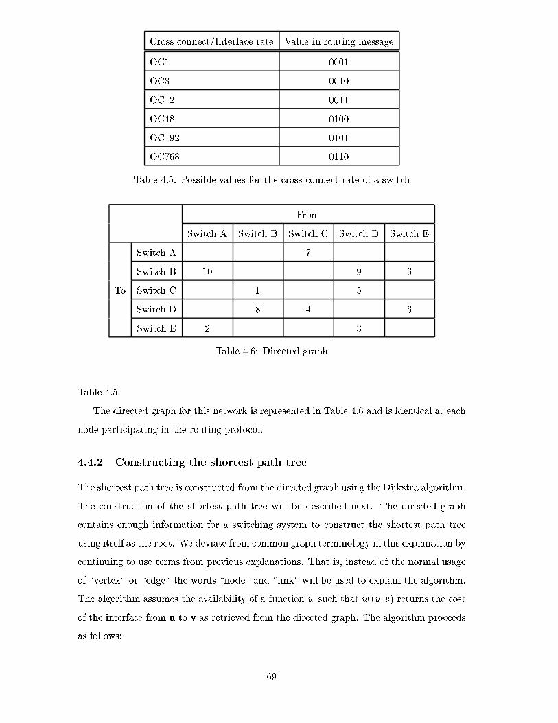
Cross connect/Interface rate Value in routing message
OC1 0001
OC3 0010
OC12 0011
OC48 0100
OC192 0101
OC768 0110
Table 4.5: Possible values for the cross connect rate of a switch
From
Switch A Switch B Switch C Switch D Switch E
Switch A 7
Switch B 10 9 6
To Switch C 1 5
Switch D 8 4 6
Switch E 2 3
Table 4.6: Directed graph
Table 4.5.
The directed graph for this network is represented in Table 4.6 and is identical at each
node participating in the routing protocol.
4.4.2 Constructing the shortest path tree
The shortest path tree is constructed from the directed graph using the Dijkstra algorithm.
The construction of the shortest path tree will be described next. The directed graph
contains enough information for a switching system to construct the shortest path tree
using itself as the root. We deviate from common graph terminology in this explanation by
continuing to use terms from previous explanations. That is, instead of the normal usage
of \vertex" or \edge" the words \node" and \link" will be used to explain the algorithm.
The algorithm assumes the availability of a function w such that w (u; v) returns the cost
of the interface from u to v as retrieved from the directed graph. The algorithm proceeds
as follows:
69
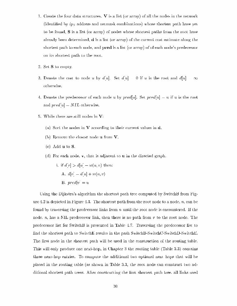
1. Create the four data structures. V is a list (or array) of all the nodes in the network
(identi�ed by ipS address and netmask combinations) whose shortest path have yet
to be found, S is a list (or array) of nodes whose shortest paths from the root have
already been determined, d is a list (or array) of the current cost estimate along the
shortest path to each node, and pred is a list (or array) of of each node's predecessor
on its shortest path to the root.
2. Set S to empty.
3. Denote the cost to node u by d[u]. Set d[u] = 0 if u is the root and d[u] = 1
otherwise.
4. Denote the predecessor of each node u by pred[u]. Set pred[u] = u if u is the root
and pred[u] = NIL otherwise.
5. While there are still nodes in V:
(a) Sort the nodes in V according to their current values in d.
(b) Remove the closest node u from V.
(c) Add u to S.
(d) For each node, v, that is adjacent to u in the directed graph.
i. if d[v] > d[u] + w(u; v) then:
A. d[v] = d[u] + w(u; v)
B. pred[v] = u
Using the Dijkstra's algorithm the shortest path tree computed by SwitchB from Fig-
ure 4.2 is depicted in Figure 4.3. The shortest path from the root node to a node, n, can be
found by traversing the predecessor links from n until the root node is encountered. If the
node, n, has a NIL predecessor link, then there is no path from x to the root node. The
predecessor list for SwitchB is presented in Table 4.7. Traversing the predecessor list to
�nd the shortest path to SwitchE results in the path SwitchB-SwitchC-SwitchD-SwitchE.
The �rst node in the shortest path will be used in the construction of the routing table.
This will only produce one next-hop, in Chapter 3 the routing table (Table 3.3) contains
three next-hop entries. To compute the additional two optional next hops that will be
placed in the routing table (as shown in Table 3.3, the root node can construct two ad-
ditional shortest path trees. After constructing the �rst shortest path tree, all links used
70
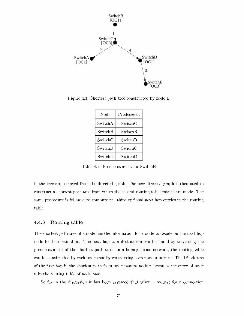
1
7 4
3
[OC1]
[OC3]
[OC1]SwitchA[OC1]
SwitchC
SwitchB
SwitchD
SwitchE[OC3]
Figure 4.3: Shortest path tree constructed by node B
Node Predecessor
SwitchA SwitchC
SwitchB SwitchB
SwitchC SwitchB
SwitchD SwitchC
SwitchE SwitchD
Table 4.7: Predecessor list for SwitchB
in the tree are removed from the directed graph. The new directed graph is then used to
construct a shortest path tree from which the second routing table entries are made. The
same procedure is followed to compute the third optional next hop entries in the routing
table.
4.4.3 Routing table
The shortest path tree of a node has the information for a node to decide on the next hop
node to the destination. The next hop to a destination can be found by traversing the
predecessor list of the shortest path tree. In a homogeneous network, the routing table
can be constructed by each node root by considering each node n in turn. The IP address
of the �rst hop in the shortest path from node root to node n becomes the entry of node
n in the routing table of node root.
So far in the discussion it has been assumed that when a request for a connection
71
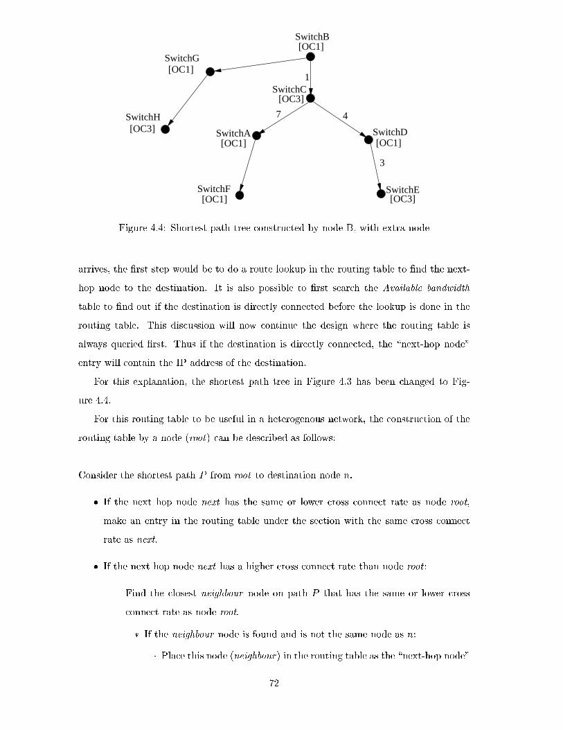
1
7 4
3
[OC1]
[OC3]
[OC1]SwitchA[OC1]
SwitchC
SwitchB
SwitchD
SwitchE[OC3][OC1]
SwitchF
[OC1]SwitchG
[OC3]SwitchH
Figure 4.4: Shortest path tree constructed by node B, with extra node
arrives, the �rst step would be to do a route lookup in the routing table to �nd the next-
hop node to the destination. It is also possible to �rst search the Available bandwidth
table to �nd out if the destination is directly connected before the lookup is done in the
routing table. This discussion will now continue the design where the routing table is
always queried �rst. Thus if the destination is directly connected, the \next-hop node"
entry will contain the IP address of the destination.
For this explanation, the shortest path tree in Figure 4.3 has been changed to Fig-
ure 4.4.
For this routing table to be useful in a heterogenous network, the construction of the
routing table by a node (root) can be described as follows:
Consider the shortest path P from root to destination node n.
� If the next hop node next has the same or lower cross connect rate as node root,
make an entry in the routing table under the section with the same cross connect
rate as next.
� If the next hop node next has a higher cross connect rate than node root :
{ Find the closest neighbour node on path P that has the same or lower cross
connect rate as node root.
� If the neighbour node is found and is not the same node as n:
� Place this node (neighbour) in the routing table as the \next-hop node"
72

used to reach node n. This entry is made at the crossconnect rate of
neighbour.
� Search the path from root to neighbour for the node with the highest
cross connect rate (highrate).
� Place next in the routing table as the next-hop node to reach neighbour.
This entry is made at the cross connect rate section highrate.
� If the neighbour node turns out to be n or if no neighbour node is found:
� Search for the node with the highest cross connect on path P
� Place the entry for the next hop node next in the routing table at this
cross connect rate section.
When SwitchB constructs the routing table according to the shortest path tree depicted
in Figure 4.4, it will proceed as follows. The �rst node it considers is SwitchC, which has
a higher cross connect rate than SwitchB. As explained above, SwitchB shall search the
path to SwitchC for a neighbour, there is no neighbour on this path, and the highest cross
connect rate is OC3 - so an entry for SwitchC will be made in the routing table block
under the rate OC3. Next, consider node SwitchF. Again, the next hop node (SwitchC)
has a higher cross connect rate than SwitchB. Searching the path for a node that has
the same or lower cross connect rate than SwitchB reveals that SwitchA is the neighbour,
an entry is made in the routing table indicating that SwitchA is the \next-hop node"
to SwitchF. Searching for the node with the highest cross connect rate on the path to
SwitchA produces SwitchC. So, an entry in the OC3 section will indicate that SwitchC is
the \next-hop node" for SwitchA. The resulting routing table for SwitchB in Figure 4.4 is
presented in Table 4.8.
Another example network is depicted in Figure 4.5. This example network contains
a path that is similar to the path describing the signaling protocol's operation in a het-
erogenous network given in Chapter 3. The path from Switch3 to Switch6 discussed in
Section 3.9.1 can be found in Figure 4.5. The corresponding routing table is given in
Table 4.9.
4.5 Future work
The segmentation of the network is a functionality that is required in a routing protocol
when it operates in a large network. Without network segmentation the routing databases
73
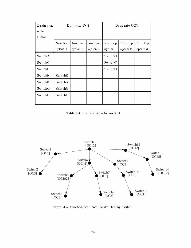
Destination
node
address
Data rate OC1 Data rate OC3
Next hop
option 1
Next hop
option 2
Next hop
option 3
Next hop
option 1
Next hop
option 2
Next hop
option 3
SwitchA SwitchC
SwitchC SwitchC
SwitchD SwitchC
SwitchE SwitchD
SwitchF SwitchA
SwitchG SwitchG
SwitchH SwitchG
Table 4.8: Routing table for node B
Switch3
[OC1]
[OC3]
Switch4
Switch5
Switch6
[OC12]
[OC3]
Switch1
Switch2
Switch8[OC3]
Switch7[OC1]
Switch9
Switch10
Switch11
Switch12
Switch13
Switch14
[OC3]
[OC3]
[OC1]
[OC48]
[OC12]
[OC12]
[OC192]
[OC48]
Figure 4.5: Shortest path tree constructed by Switch3
74
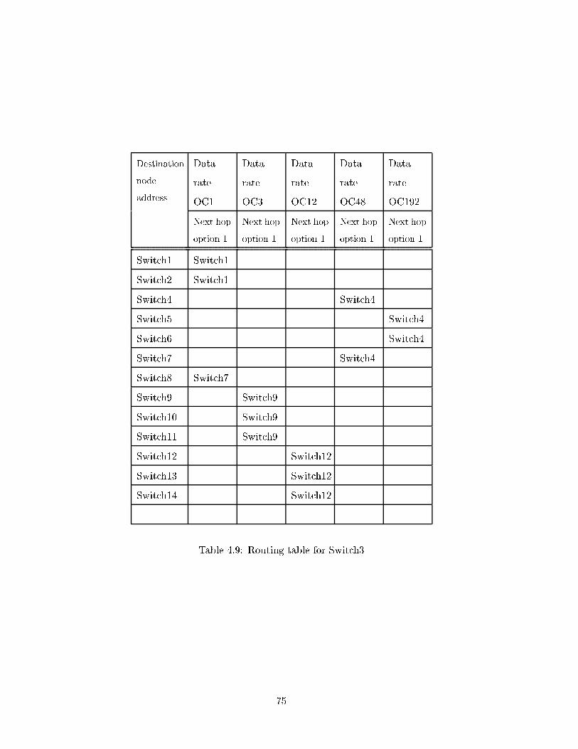
Destination
node
address
Data
rate
OC1
Data
rate
OC3
Data
rate
OC12
Data
rate
OC48
Data
rate
OC192
Next hop
option 1
Next hop
option 1
Next hop
option 1
Next hop
option 1
Next hop
option 1
Switch1 Switch1
Switch2 Switch1
Switch4 Switch4
Switch5 Switch4
Switch6 Switch4
Switch7 Switch4
Switch8 Switch7
Switch9 Switch9
Switch10 Switch9
Switch11 Switch9
Switch12 Switch12
Switch13 Switch12
Switch14 Switch12
Table 4.9: Routing table for Switch3
75
tend to grow very large. Despite route precomputation being used, this step (route pre-
computation) could still consume a lot of resources, even if nodes only exchange a small
number of routing updates. The �rst step in adding his functionality would be to spec-
ify the usage of IP addresses in the network segments, and secondly, the creation of the
routing table has to be re-examined. The costs advertised between network segments will
contain summaries of the cost values in the particular network segment - the next hop
entry in the routing table should now contain the next hop to a network path that is most
likely to be able to handle the connection based on more relaxed parameters that basic
CAC.
In Section 3.9.1 an improvement to the routing protocol was brie y mentioned. The
second improvement to the routing protocol concerns connections that have already been
set up between switches in the form of logical links (links that have been used to set
up lower rate connections over switches with high cross connect rates) and provisioned
connections. An improvement to the routing protocol would be to exchange information
regarding available bandwidth on connections that have already been set up, not just
available bandwidth of the interfaces. For example, if a unidirectional OC12 connection is
set up between two switches (from switch I to switch I+1), and only one OC1 connection
is currently active on it, switch I can advertise that it is directly connected to switch I+1
(even if there are switches between them), and the cost of the link is again a function of
the available bandwidth of the connection.
76
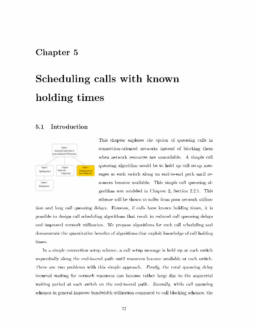
Chapter 5
Scheduling calls with known
holding times
5.1 Introduction
Chapter 2Analyzing file transfer delays in
circuit-switched and TCP/IP networks.
Chapter 6Further work:
Transport layer
Chapter 3
Signaling protocol
Chapter 5Scheduling calls with known holding times
Chapter 4
Routing protocol
This chapter explores the option of queueing calls in
connection-oriented networks instead of blocking them
when network resources are unavailable. A simple call
queueing algorithm would be to hold up call setup mes-
sages at each switch along an end-to-end path until re-
sources become available. This simple call queueing al-
gorithm was modeled in Chapter 2, Section 2.2.1. This
scheme will be shown to su�er from poor network utiliza-
tion and long call queueing delays. However, if calls have known holding times, it is
possible to design call scheduling algorithms that result in reduced call queueing delays
and improved network utilization. We propose algorithms for such call scheduling and
demonstrate the quantitative bene�ts of algorithms that exploit knowledge of call holding
times.
In a simple connection setup scheme, a call setup message is held up at each switch
sequentially along the end-to-end path until resources become available at each switch.
There are two problems with this simple approach. Firstly, the total queueing delay
incurred waiting for network resources can become rather large due to the sequential
waiting period at each switch on the end-to-end path. Secondly, while call queueing
schemes in general improve bandwidth utilization compared to call blocking schemes, the
77
kTwait scheme will not achieve the maximum improvement possible. The kTwait scheme
was �rst used in Miyahara et al's paper [7] for the comparison between circuit-switching
and CL packet-switching for large �le transfers. In this scheme the signaling message
requesting the connection is placed in a queue at each switch to wait for the required
resources to be released. Only when the connection request reaches the head of the queue,
and its requested resources are available, will the request be passed on to the next switch.
Hence the term kTwait. The reason an improvement in bandwidth utilization can be
expected in call queueing schemes is that by having bu�ers to queue calls, less bandwidth
is needed than for a strictly call blocking scheme. The reason why the kTwait scheme does
not take full advantage of this improvement is that upstream switches hold resources while
waiting for downstream switches to admit a call instead of using the wait period to admit
shorter calls that only traverse upstream segments.
To overcome these two problems, we started looking for ways to improve the call
queueing algorithm. This led us to consider options where the switches agree upon a
delayed start time for a given call c, and allow other calls sharing segments of the end-to-
end path of call c to use the network resources for other calls before call c starts. This
would decrease call queueing delays and allow for the utilization gains of call queueing to
be realized. However, scheduling calls for a delayed start time with mutual agreement at
all the switches on the end-to-end path is only possible if call holding times are known.
A switch cannot guarantee that resources will be available for a new call c at some later
point in time if it does not know when existing calls will complete. Hence, we focus on the
call queueing/scheduling problem for calls with known holding times that can be identi�ed
when satisfying the following two characteristics:
� The data from the sending end of the call should be \stored," as opposed to \live."
� The CO network should use preventive congestion control as opposed to reactive.
We continued to design a call scheduling algorithm when call holding times are known.
Such an algorithm could coexist with a traditional call admission control algorithm for
calls with unknown holding times by partitioning network resources for calls with known
holding times from resources for calls with unknown holding times.
This proposed method for scheduling connections can be used in any type of
connection-oriented (CO) network. CO networks are networks where resources are re-
served for a connection between end hosts before any data transmission may start. These
78
networks can either be packet-switched (for example ATM or X.25 networks) or circuit-
switched (for example SONET or WDM networks).
The motivating applications for such an algorithm are described in in Section 5.2.
Section 5.3 describes the proposed algorithm as applied to a simple one-switch network,
Section 5.4 continues by explaining some extensions to the algorithm, which includes the
algorithm's behaviour in a network where multiple switches are involved. Some solutions to
the distributed computing problem are proposed in Section 5.5 and Section 5.6 provides
the results of simulations run to determine the feasibility of the solutions. Section 5.7
introduces some problems that still need to be solved. Conclusions are made in Section 5.8.
5.2 Motivating applications
While the motivation for this work came from our interest in supporting end-to-end
large �le transfers on high-speed circuit-switched networks, we considered the question
of whether there are other applications for which call holding times are known. Two
characteristics of calls have been identi�ed that allows us to determine the call holding
time:
� The data from the sending end of the call should be \stored," as opposed to \live."
� The CO network should use preventive congestion control as opposed to reactive.
Consider the �rst characteristic. Table 5.1 shows that the sending end and consuming end
of any two-party (as opposed to multi-party) data transfer can each be \live" or \stored."
If both ends are live and the communication is bidirectional, we classify such sessions
as interactive. An example of this category is telephony, where the call holding time is
unknown. Given that both ends are \live" and both ends can send traÆc, the call could
hold for any length of time. If both ends are live, but the communication is unidirectional,
we refer to this case as a live streaming data transfer. An example is listening to/viewing
a live radio/TV broadcast. The next category shown in Table 5.1 is recording, where
the source is live, but the receiver is a storing device. In both the live streaming and
recording categories, the call holding time may or may not be known since it depends on
the duration of the live \event." For e.g., the duration of coverage of a live parade could
be known a priori and advertised by the audio/video distributor; on the other hand, the
duration of a sporting event, for e.g., a tennis match, is not known beforehand. Therefore,
in general we assume that if the sending end is \live," call holding times are unknown.
79
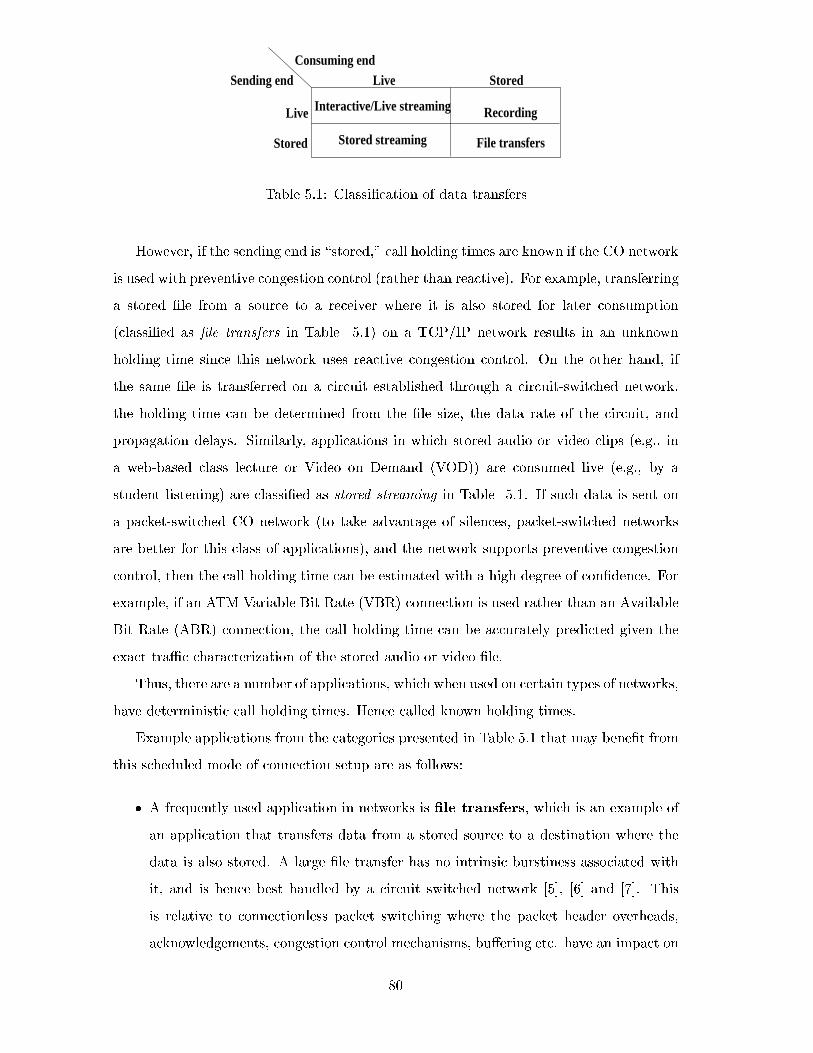
Recording
Sending endConsuming end
Live Stored
Stored
Live
File transfersStored streaming
Interactive/Live streaming
Table 5.1: Classi�cation of data transfers
However, if the sending end is \stored," call holding times are known if the CO network
is used with preventive congestion control (rather than reactive). For example, transferring
a stored �le from a source to a receiver where it is also stored for later consumption
(classi�ed as �le transfers in Table 5.1) on a TCP/IP network results in an unknown
holding time since this network uses reactive congestion control. On the other hand, if
the same �le is transferred on a circuit established through a circuit-switched network,
the holding time can be determined from the �le size, the data rate of the circuit, and
propagation delays. Similarly, applications in which stored audio or video clips (e.g., in
a web-based class lecture or Video on Demand (VOD)) are consumed live (e.g., by a
student listening) are classi�ed as stored streaming in Table 5.1. If such data is sent on
a packet-switched CO network (to take advantage of silences, packet-switched networks
are better for this class of applications), and the network supports preventive congestion
control, then the call holding time can be estimated with a high degree of con�dence. For
example, if an ATM Variable Bit Rate (VBR) connection is used rather than an Available
Bit Rate (ABR) connection, the call holding time can be accurately predicted given the
exact traÆc characterization of the stored audio or video �le.
Thus, there are a number of applications, which when used on certain types of networks,
have deterministic call holding times. Hence called known holding times.
Example applications from the categories presented in Table 5.1 that may bene�t from
this scheduled mode of connection setup are as follows:
� A frequently used application in networks is �le transfers, which is an example of
an application that transfers data from a stored source to a destination where the
data is also stored. A large �le transfer has no intrinsic burstiness associated with
it, and is hence best handled by a circuit switched network [5], [6] and [7]. This
is relative to connectionless packet switching where the packet header overheads,
acknowledgements, congestion control mechanisms, bu�ering etc. have an impact on
80
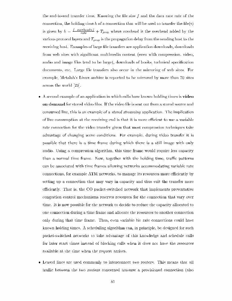
the end-to-end transfer time. Knowing the �le size f and the data rate rate of the
connection, the holding time h of a connection that will be used to transfer the �le(s)
is given by h = f+overhead�frate
+ Tprop where overhead is the overhead added by the
various protocol layers and Tprop is the propagation delay from the sending host to the
receiving host. Examples of large �le transfers are application downloads, downloads
from web sites with signi�cant multimedia content (even with compression, video,
audio and image �les tend to be large), downloads of books, technical speci�cation
documents, etc. Large �le transfers also occur in the mirroring of web sites. For
example, Metalab's Linux archive is reported to be mirrored by more than 70 sites
across the world [23].
� A second example of an application in which calls have known holding times is video
on demand for stored video �les. If the video �le is sent out from a stored source and
consumed live, this is an example of a stored streaming application. The implication
of live consumption at the receiving end is that it is more eÆcient to use a variable
rate connection for the video transfer given that most compression techniques take
advantage of changing scene conditions. For example, during video transfer it is
possible that there is a time frame during which there is a still image with only
audio. Using a compression algorithm, this time frame would require less capacity
than a normal time frame. Now, together with the holding time, traÆc patterns
can be associated with time frames allowing networks accommodating variable rate
connections, for example ATM networks, to manage its resources more eÆciently by
setting up a connection that may vary in capacity and thus suit the transfer more
eÆciently. That is, the CO packet-switched network that implements preventative
congestion control mechanisms reserves resources for the connection that vary over
time. It is now possible for the network to decide to reduce the capacity allocated to
one connection during a time frame and allocate the resources to another connection
only during that time frame. Thus, even variable bit rate connections could have
known holding times. A scheduling algorithm can, in principle, be designed for such
packet-switched networks to take advantage of this knowledge and schedule calls
for later start times instead of blocking calls when it does not have the resources
available at the time when the request arrives.
� Leased lines are used commonly to interconnect two routers. This means that all
traÆc between the two routers concerned traverse a provisioned connection (also
81
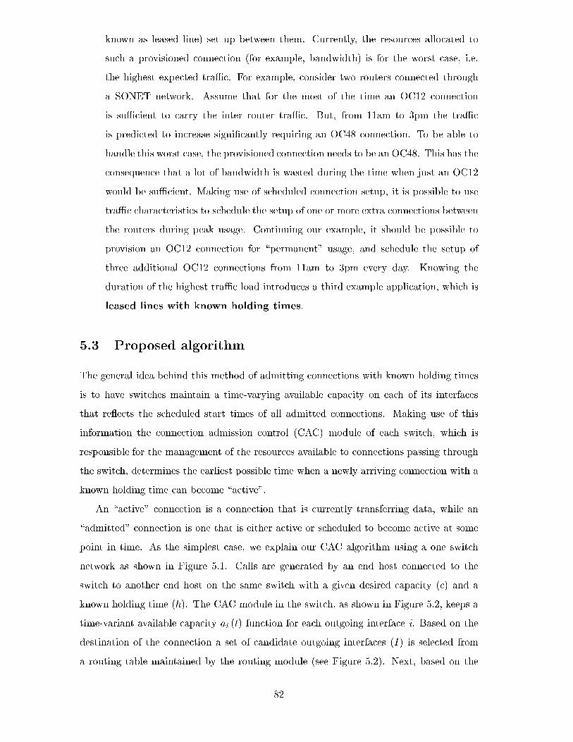
known as leased line) set up between them. Currently, the resources allocated to
such a provisioned connection (for example, bandwidth) is for the worst case, i.e.
the highest expected traÆc. For example, consider two routers connected through
a SONET network. Assume that for the most of the time an OC12 connection
is suÆcient to carry the inter router traÆc. But, from 11am to 3pm the traÆc
is predicted to increase signi�cantly requiring an OC48 connection. To be able to
handle this worst case, the provisioned connection needs to be an OC48. This has the
consequence that a lot of bandwidth is wasted during the time when just an OC12
would be suÆcient. Making use of scheduled connection setup, it is possible to use
traÆc characteristics to schedule the setup of one or more extra connections between
the routers during peak usage. Continuing our example, it should be possible to
provision an OC12 connection for \permanent" usage, and schedule the setup of
three additional OC12 connections from 11am to 3pm every day. Knowing the
duration of the highest traÆc load introduces a third example application, which is
leased lines with known holding times.
5.3 Proposed algorithm
The general idea behind this method of admitting connections with known holding times
is to have switches maintain a time-varying available capacity on each of its interfaces
that re ects the scheduled start times of all admitted connections. Making use of this
information the connection admission control (CAC) module of each switch, which is
responsible for the management of the resources available to connections passing through
the switch, determines the earliest possible time when a newly arriving connection with a
known holding time can become \active".
An \active" connection is a connection that is currently transferring data, while an
\admitted" connection is one that is either active or scheduled to become active at some
point in time. As the simplest case, we explain our CAC algorithm using a one switch
network as shown in Figure 5.1. Calls are generated by an end host connected to the
switch to another end host on the same switch with a given desired capacity (c) and a
known holding time (h). The CAC module in the switch, as shown in Figure 5.2, keeps a
time-variant available capacity ai (t) function for each outgoing interface i. Based on the
destination of the connection a set of candidate outgoing interfaces (I ) is selected from
a routing table maintained by the routing module (see Figure 5.2). Next, based on the
82
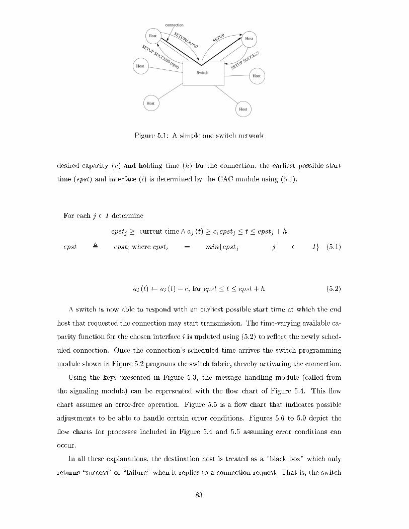
Switch
Host
Host
HostHost
Host
HostSETUP
SETUP SUCCESS
SETUP SUCCESS (epst)
connection
SETUP(c,h,req)
Figure 5.1: A simple one switch network
desired capacity (c) and holding time (h) for the connection, the earliest possible start
time (epst) and interface (i) is determined by the CAC module using (5.1).
For each j 2 I determine
epstj � current time ^ aj (t) � c; epstj � t � epstj + h
epst , epsti where epsti = minfepstj j j 2 Ig (5.1)
ai (t) ai (t)� c, for epst � t � epst+ h (5.2)
A switch is now able to respond with an earliest possible start time at which the end
host that requested the connection may start transmission. The time-varying available ca-
pacity function for the chosen interface i is updated using (5.2) to re ect the newly sched-
uled connection. Once the connection's scheduled time arrives the switch programming
module shown in Figure 5.2 programs the switch fabric, thereby activating the connection.
Using the keys presented in Figure 5.3, the message handling module (called from
the signaling module) can be represented with the ow chart of Figure 5.4. This ow
chart assumes an error-free operation. Figure 5.5 is a ow chart that indicates possible
adjustments to be able to handle certain error conditions. Figures 5.6 to 5.9 depict the
ow charts for processes included in Figure 5.4 and 5.5 assuming error conditions can
occur.
In all these explanations, the destination host is treated as a \black box" which only
returns \success" or \failure" when it replies to a connection request. That is, the switch
83
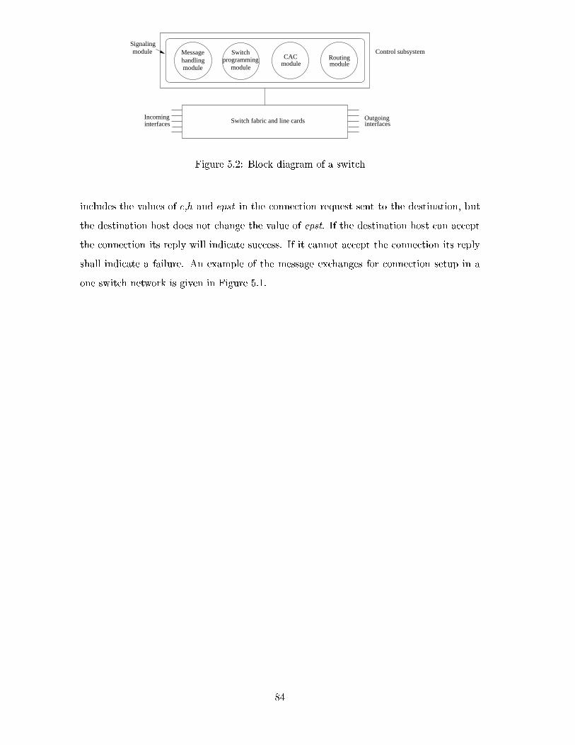
Signalingmodule
Routingmodule
CACmodule
Switchprogramming
module
Messagehandlingmodule
interfacesOutgoing
Control subsystem
Incominginterfaces Switch fabric and line cards
Figure 5.2: Block diagram of a switch
includes the values of c,h and epst in the connection request sent to the destination, but
the destination host does not change the value of epst. If the destination host can accept
the connection its reply will indicate success. If it cannot accept the connection its reply
shall indicate a failure. An example of the message exchanges for connection setup in a
one switch network is given in Figure 5.1.
84
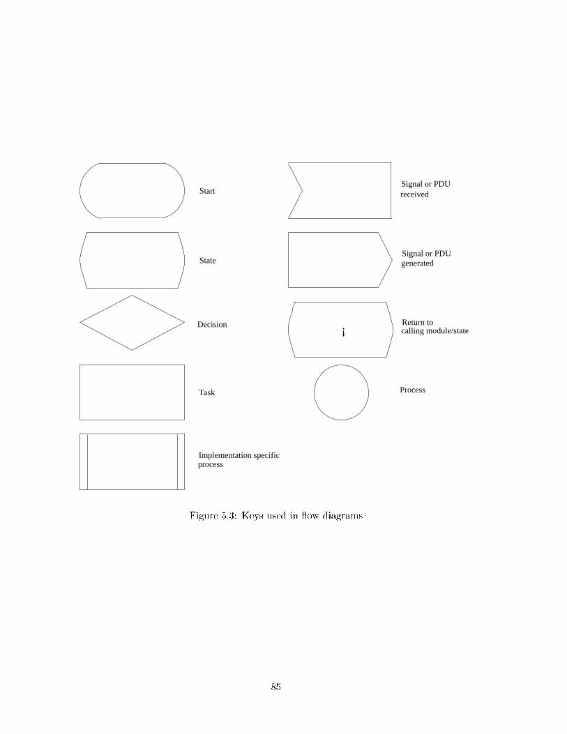
!
Start
State
Decision
Task
Implementation specificprocess
Signal or PDU received
Signal or PDUgenerated
Return to
Process
calling module/state
Figure 5.3: Keys used in ow diagrams
85

lookupRoute
Scheduleconnection
(CAC)
Pass connection requeston to next hop, include
Receive success reply
1
Send success reply tohost requesting the con-nection. Include value ofepst.
2values for c, h and epst
current time < epst ?
Yes
No
Programswitch
Connection active
arrives with requestedcapacity (c) and holdingtime (h).
returned.
destination address (d).do a route lookup for Invoke routing module to
A set of interfaces (I) is
Handleincomingmessages
Message handling modulehas been invoked by thesignaling module to handleconnection setup request.
to schedule connection.Invoke CAC module
Invoke switch programmingmodule to program theswitch fabric.
!
Return with success tothe signaling module.
Request for new connec-tion (n) to destination (d)
Figure 5.4: Flow chart for the message handling module in a one switch network
86
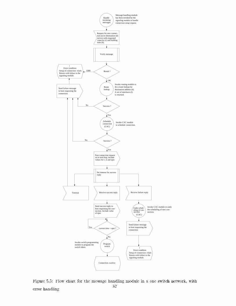
Setup of connection fails
!
Error condition
signaling module.Return with failure to the
n
Setup of connection fails
!
Error condition
signaling module.Return with failure to the
n
Verify message
Result ?ERR
OK
Routelookup
Success ?No
Yes
Scheduleconnection
(CAC)
Success ?No
Yes
Pass connection requeston to next hop, include
reply
Receive success replyTimeout
Send success reply tohost requesting the con-nection. Include valueof epst.
Receive failure reply
current time < epst ?Yes
No
switchProgram
Undo sched-uling of con-nection
(CAC)
Send failure messageto host requesting theconnection
Send failure messageto host requesting theconnection
messagesincomingHandle
Message handling modulehas been invoked by thesignaling module to handleconnection setup request.
Request for new connec-tion (n) to destination (d)arrives with requestedcapacity (c) and holdingtime (h).
Invoke routing module todo a route lookup fordestination address (d). A set of interfaces (I)is returned.
Invoke CAC moduleto schedule connection.
Set timeout for success
Invoke CAC module to undo the scheduling of new con-nection.
Invoke switch programmingmodule to program the switch fabric.
Connection activen
values for c, h and epst.
Figure 5.5: Flow chart for the message handling module in a one switch network, with
error handling87
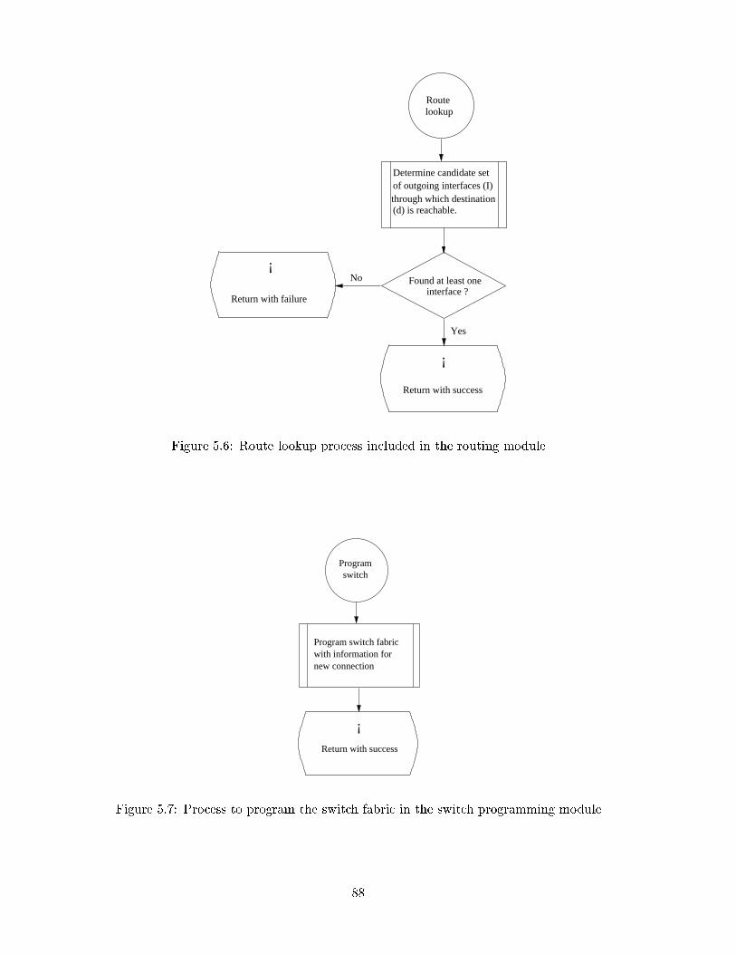
Routelookup
!
!
Return with failure
Return with success
Yes
No
Determine candidate setof outgoing interfaces (I)through which destination(d) is reachable.
Found at least oneinterface ?
Figure 5.6: Route lookup process included in the routing module
!
Return with success
Programswitch
Program switch fabricwith information for new connection
Figure 5.7: Process to program the switch fabric in the switch programming module
88

!
Return with failure
Yes
No
Scheduleconnection
(CAC)
epst found ?
from epst until epst+hReserve capacity c
!
Return with success
Compute epst for connec- 1
2
available capacity function
ted within set I.i i
tion using (5.1)
a (t) for interface selec-
update time variant Using (5.2),
Figure 5.8: Scheduling process included in the CAC module for a one switch network
89
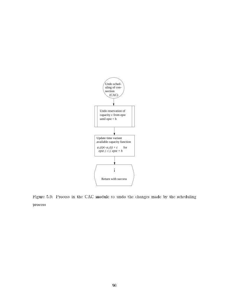
!
Return with success
Undo sched-uling of con-nection
(CAC)
Undo reservation of capacity c from epst until epst + h
Update time variantavailable capacity function
foriepst < t < epst + h
ia (t) a (t) + c
Figure 5.9: Process in the CAC module to undo the changes made by the scheduling
process
90
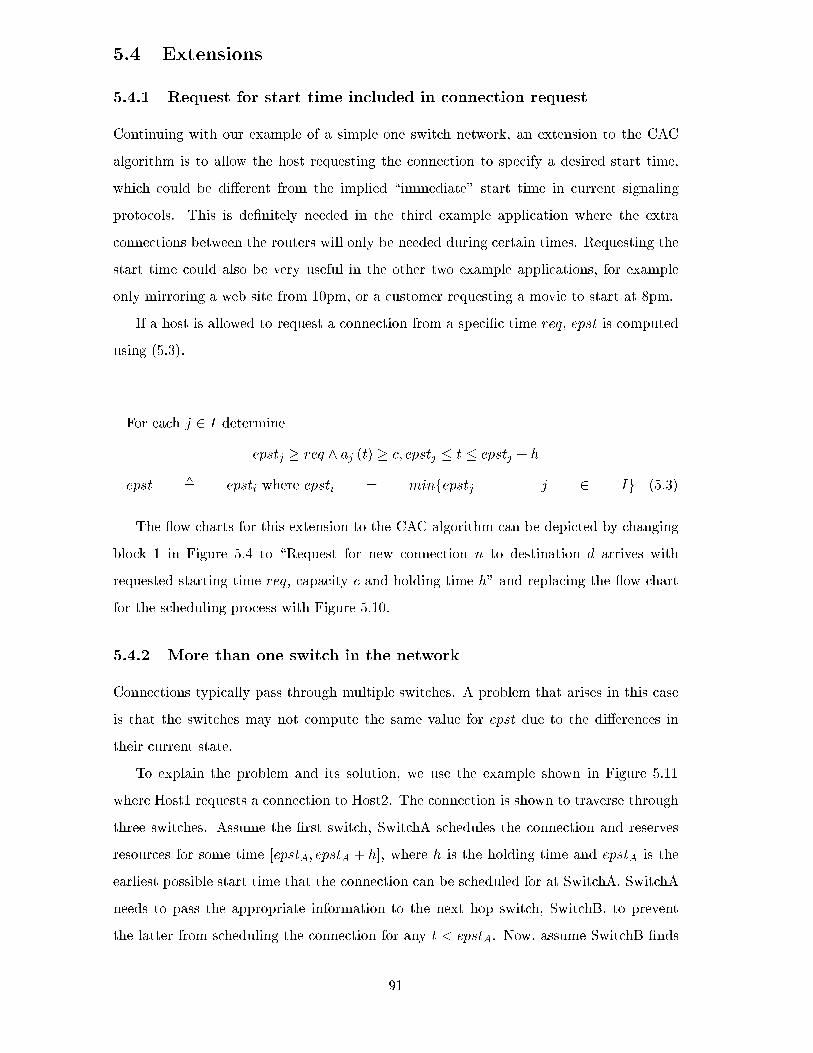
5.4 Extensions
5.4.1 Request for start time included in connection request
Continuing with our example of a simple one switch network, an extension to the CAC
algorithm is to allow the host requesting the connection to specify a desired start time,
which could be di�erent from the implied \immediate" start time in current signaling
protocols. This is de�nitely needed in the third example application where the extra
connections between the routers will only be needed during certain times. Requesting the
start time could also be very useful in the other two example applications, for example
only mirroring a web site from 10pm, or a customer requesting a movie to start at 8pm.
If a host is allowed to request a connection from a speci�c time req, epst is computed
using (5.3).
For each j 2 I determine
epstj � req ^ aj (t) � c; epstj � t � epstj + h
epst , epsti where epsti = minfepstj j j 2 Ig (5.3)
The ow charts for this extension to the CAC algorithm can be depicted by changing
block 1 in Figure 5.4 to \Request for new connection n to destination d arrives with
requested starting time req, capacity c and holding time h" and replacing the ow chart
for the scheduling process with Figure 5.10.
5.4.2 More than one switch in the network
Connections typically pass through multiple switches. A problem that arises in this case
is that the switches may not compute the same value for epst due to the di�erences in
their current state.
To explain the problem and its solution, we use the example shown in Figure 5.11
where Host1 requests a connection to Host2. The connection is shown to traverse through
three switches. Assume the �rst switch, SwitchA schedules the connection and reserves
resources for some time [epstA; epstA + h], where h is the holding time and epstA is the
earliest possible start time that the connection can be scheduled for at SwitchA. SwitchA
needs to pass the appropriate information to the next hop switch, SwitchB, to prevent
the latter from scheduling the connection for any t < epstA. Now, assume SwitchB �nds
91
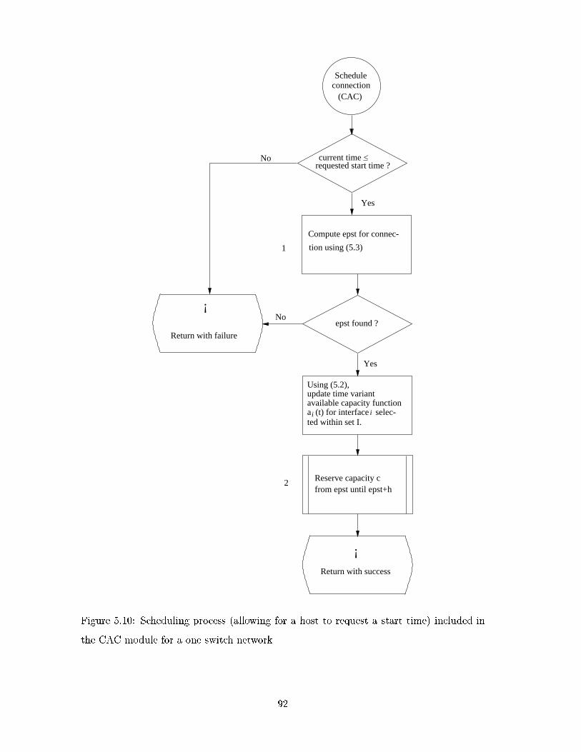
Scheduleconnection
(CAC)
requested start time ?
Compute epst for connec-
!
Return with failure
Yes
Noepst found ?
from epst until epst+hReserve capacity c
!
Return with success
1
2
No
Yes
current time <
update time variantavailable capacity function
ted within set I.ia (t) for interface selec-i
tion using (5.3)
Using (5.2),
Figure 5.10: Scheduling process (allowing for a host to request a start time) included in
the CAC module for a one switch network
92
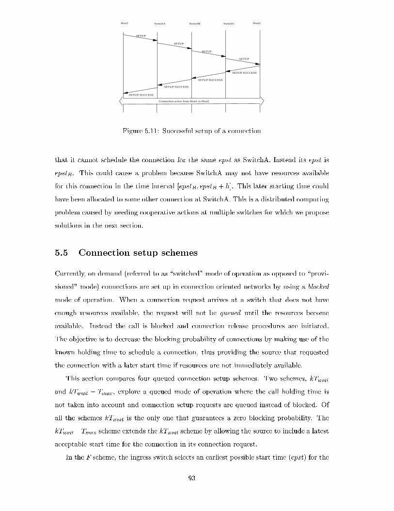
SETUP
SETUP
SETUP
SETUP
Host1 SwitchA SwitchB SwitchC Host2
SETUP SUCCESS
SETUP SUCCESS
SETUP SUCCESS
SETUP SUCCESS
Connection active from Host1 to Host2
Figure 5.11: Successful setup of a connection
that it cannot schedule the connection for the same epst as SwitchA. Instead its epst is
epstB. This could cause a problem because SwitchA may not have resources available
for this connection in the time interval [epstB; epstB + h]. This later starting time could
have been allocated to some other connection at SwitchA. This is a distributed computing
problem caused by needing cooperative actions at multiple switches for which we propose
solutions in the next section.
5.5 Connection setup schemes
Currently, on demand (referred to as \switched" mode of operation as opposed to \provi-
sioned" mode) connections are set up in connection-oriented networks by using a blocked
mode of operation. When a connection request arrives at a switch that does not have
enough resources available, the request will not be queued until the resources become
available. Instead the call is blocked and connection release procedures are initiated.
The objective is to decrease the blocking probability of connections by making use of the
known holding time to schedule a connection, thus providing the source that requested
the connection with a later start time if resources are not immediately available.
This section compares four queued connection setup schemes. Two schemes, kTwait
and kTwait � Tmax, explore a queued mode of operation where the call holding time is
not taken into account and connection setup requests are queued instead of blocked. Of
all the schemes kTwait is the only one that guarantees a zero blocking probability. The
kTwait�Tmax scheme extends the kTwait scheme by allowing the source to include a latest
acceptable start time for the connection in its connection request.
In the F scheme, the ingress switch selects an earliest possible start time (epst) for the
93
connection such that is has resources available for the connection from epst to epst+h+F ,
where h is the holding time of the call and F is some large time value. It holds the resources
for this connection for this large time period hoping that the downstream switches will
select an epst within this large time period. If a large enough value of F is selected, the
probability of success will be high.
In the timeslots scheme, the ingress switch selects multiple time ranges during which
it can accommodate the call. Each downstream switch checks to see if it has available
resources for one or more of these time ranges. Each switch along the path may narrow
the time ranges until �nally there exists at least one common time range (of length equal
to the call holding time) during which the required resources are available at all switches.
An analogy can be drawn between these scheduling schemes and the scheduling of a
meeting involving several people. With the meeting duration known to all involved, one
way to schedule its start is for the �rst person to send out a memo stating that he/she
has \the whole of next week" available. Another solution is for the memo to read, \I
am free from 2pm to 4pm Monday, 8am to 1pm Tuesday, and the whole of the following
week." Tentatively, the sender of the memo holds these time ranges for this meeting until
a response arrives from all other participants. The �rst solution corresponds to the F
scheme and the second solution corresponds to the timeslots scheme.
The F and timeslots schemes are call queueing schemes in that calls wait for resources,
but they also block calls if the selected F value or number of time ranges is not large enough
for success. These can be augmented with negotiations (i.e., multiple signaling exchanges
on the same path), and/or searches on multiple paths to reduce call blocking probability.
5.5.1 The kTwait scheme
The kTwait scheme is the simplest queued connection setup scheme. In this scheme, switch-
es do not take call holding times into account when connections are admitted. Instead,
on receipt of a connection request it is placed in the queue of the interface that should be
used by the connection. When the bandwidth requested by the connection request at the
head of the queue becomes available, it is reserved for the connection and the connection
request is passed on to the succeeding switch, or destination host. When the connection
request reaches the destination host, a connection has already been set up from the source
to the destination. If the destination host accepts the connection, it sends a success mes-
sage back to the source. As this success message traverses the network towards the source
94
the connection is usually marked as \established". On receipt of the success message,
the source can immediately start with data transmission. If Twait is the average time a
connection request waits in a queue for resources to become available, and k indicates the
number of switches on the connection, then the term kTwait forms a large part of the total
connection setup time, hence the name kTwait as described in Chapter 2, Section 2.2.1.
5.5.2 The kTwait � Tmax scheme
The second queued connection setup scheme is designed by slightly modifying the kTwait
scheme. When sending a connection request to its ingress switch, a source host might
expect the connection to be established before a certain time. For example, the source host
might request that a connection be established at most 50 seconds from when it requested
it. This connection setup scheme also does not take the holding time into account when a
connection is set up, but provides the source requesting the connection some control over
the start time of the connection, hence named the kTwait�Tmax connection setup scheme.
The kTwait � Tmax scheme works in the same manner as the kTwait scheme except that
the source host is allowed to include a time, Tmax, in its connection request. The value
of Tmax indicates the latest possible time that the source would accept as a start time
for this connection. As in the kTwait scheme, switches place a connection request in the
queue of the interface that should be used by the connection. The action taken when the
connection request is at the head of the queue, and its requested bandwidth is available,
di�ers in that the switch �rst checks if its current time is later than the time Tmax included
in the connection request. If the current time is later, connection release procedures are
initiated.
5.5.3 The F scheme
The �rst queued connection setup scheme that takes advantage of the call holding time
is called the F scheme. In this solution the requested resources are reserved for a longer
period of time than its holding time, until reverse messages are received, during the con-
nection setup procedure. In the forward phase of connection setup resources are held for
a long enough time period that if a downstream switch selects a later value for epst, there
is some likelihood that the earlier (upstream) switches of the path will have the resources
available. Resources are held for this large time period only for the short duration it takes
for the setup request to reach the destination and the reply (setup success) to return.
95
Using a large �nish time during the scheduling of a connection works as follows: a host
requests a connection from its ingress switch to a destination with the optional inclusion
of a start time; the ingress switch selects a large time range (starting with the earliest
time greater or equal to the requested start time) during which it is able to accommodate
the connection. On receipt of a time range a switch searches for the largest time range
inside the range it received from the preceding switch during which it can accommodate the
connection. This time range is included in the connection request passed to the succeeding
switch, or destination host.
The computation of epst changes in that a pre-assigned value F is added to the holding
time by the ingress switch, where F is a very large extra holding time. When a host
requests a connection to destination d from time req with capacity c and holding time
h, (5.4) can now be used at the �rst (ingress) switch to compute epst. The time-varying
available capacity function for the chosen interface is updated using (5.5) in which Tend =
epst+ h+ F .
For each j 2 I determine
epstj � req ^ aj (t) � c; epstj � t � epstj + h+ F
epst , epsti where epsti = minfepstj j j 2 Ig (5.4)
ai (t) ai (t)� c, for epst � t � Tend (5.5)
When the resources are reserved for this connection at the ingress switch, it indicates
that this connection reserves capacity c from epst to epst+h+F . To enable all the switches
in the connection to agree to the same value for epst, the value of epst, the holding time
(h) and the time Tend are included in the connection request message passed to the second
switch in the connection. The switch receiving this message shall handle this request as if
a request for a connection from time epst, as included in the connection request, has been
received.
The setup request traverses the network and each switch along the path computes
a (possibly) new value for epst and looks for the largest time period � F but � h,
during which it will have enough resources available. If found, the requested resources
are reserved for this connection (using (5.5)) for the period (epstnew, epstnew+h+Fnew),
96
and the connection request containing epstnew, Fnew + h and h are passed on to the next
hop. If a switch is unable to �nd a time period during which it can accommodate the
connection, the call is blocked and release procedures are initiated. If the destination host
accepts the request for a connection from the source, the �nal value of epst is passed from
switch to switch until the source is noti�ed of the new value of epst.
As those success reply messages traverse the network to the source, all the switches
change their resource reservation tables to re ect the new start time (the new value of
epst), and the �nish time to be epst + h. If epstlocal indicates the earliest possible start
time as computed by a switch in the forward direction of the signaling procedure, and epst
is the earliest possible start time it received in the success reply message, the time-varying
available capacity function is updated using (5.6) and (5.7).
ai (t) ai (t) + c, for epstlocal � t < epst (5.6)
ai (t) ai (t) + c, for epst+ h � t < Tend (5.7)
The ow chart for the message handling module for the ingress switch is given in
Figure 5.12. Block 1 in the scheduling process (given in Figure 5.10) changes to \Compute
epst for connection n using Equation (5.4)", and block 2 changes to \Reserve capacity c
from epst until epst + h + F.". The ow chart for the process \Update resource reservation
and a(t)" is depicted in Figure 5.13.
Figure 5.14 shows an example of scheduled connection setup using the F scheme. For
this example, the value of F is 5 hours. End host A requests a connection with a holding
time of one hour starting at 6pm, switch 1 computes that it will have enough resources
available from 6pm until 12pm, which it reserves. The setup request message traverses
the network, and every time epst is increased due to the unavailability of resources. At
switch 2 resources are reserved from 7pm until 12pm, and epst is set to 7pm. When the
setup request message reaches end host B, epst is already 9pm. End host B accepts the
connection and the success reply from switch 4 contains the �nal value of epst (9pm). As
this reply message traverses the network, each node forming part of the connection now
changes its respective resource reservations to indicate that the connection will be active
from 9pm until 10pm.
97

Send success reply tohost requesting the con-nection. Include value ofepst.
current time < epst ?
Yes
No
Programswitch
Connection active
Invoke switch programmingmodule to program theswitch fabric.
!
Return with success tothe signaling module.
lookupRoute
Scheduleconnection
(CAC)
Pass connection requeston to next hop, include
Receive success reply
1
2
arrives with requested
returned.
destination address (d).do a route lookup for Invoke routing module to
A set of interfaces (I) is
Handleincomingmessages
Message handling modulehas been invoked by thesignaling module to handleconnection setup request.
to schedule connection.Invoke CAC module
Request for new connec-tion (n) to destination (d)
capacity (c), holding time (h), start time (req).
(CAC)vation and a(t)source reser-Update re-
to update the schedulinginformation.
Invoke CAC module
values for c, h, epst and Tend
Figure 5.12: Connection setup at the ingress switch of a connection (F scheme)
98
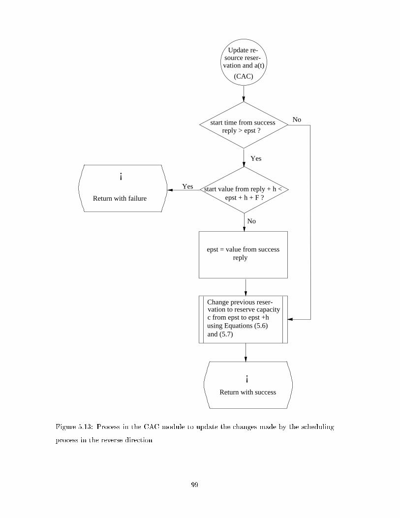
!
Return with failure
Return with success
!
Update re-
vation and a(t)source reser-
(CAC)
reply
start time from success
Yes
epst + h + F ?
Yes
No
epst = value from success
No
reply > epst ?
start value from reply + h <
Change previous reser-vation to reserve capacityc from epst to epst +husing Equations (5.6)and (5.7)
Figure 5.13: Process in the CAC module to update the changes made by the scheduling
process in the reverse direction
99
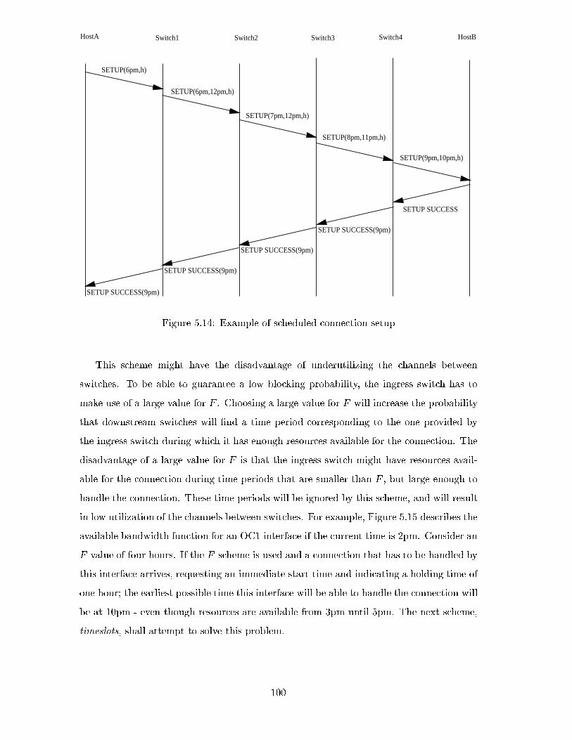
HostA Switch1 Switch2 Switch3 Switch4 HostB
SETUP SUCCESS(9pm)
SETUP SUCCESS(9pm)
SETUP SUCCESS(9pm)
SETUP SUCCESS(9pm)
SETUP(6pm,h)
SETUP SUCCESS
SETUP(6pm,12pm,h)
SETUP(7pm,12pm,h)
SETUP(8pm,11pm,h)
SETUP(9pm,10pm,h)
Figure 5.14: Example of scheduled connection setup
This scheme might have the disadvantage of underutilizing the channels between
switches. To be able to guarantee a low blocking probability, the ingress switch has to
make use of a large value for F . Choosing a large value for F will increase the probability
that downstream switches will �nd a time period corresponding to the one provided by
the ingress switch during which it has enough resources available for the connection. The
disadvantage of a large value for F is that the ingress switch might have resources avail-
able for the connection during time periods that are smaller than F , but large enough to
handle the connection. These time periods will be ignored by this scheme, and will result
in low utilization of the channels between switches. For example, Figure 5.15 describes the
available bandwidth function for an OC1 interface if the current time is 2pm. Consider an
F value of four hours. If the F scheme is used and a connection that has to be handled by
this interface arrives, requesting an immediate start time and indicating a holding time of
one hour; the earliest possible time this interface will be able to handle the connection will
be at 10pm - even though resources are available from 3pm until 5pm. The next scheme,
timeslots, shall attempt to solve this problem.
100
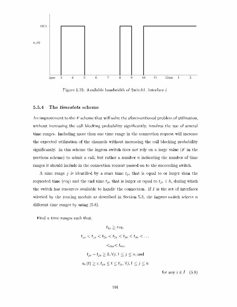
a (t)i
OC1
43 5 6 7 8 9 10 11 1 22pm 12am
Figure 5.15: Available bandwidth of Switch1, interface i
5.5.4 The timeslots scheme
An improvement to the F scheme that will solve the aforementioned problem of utilization,
without increasing the call blocking probability signi�cantly, involves the use of several
time ranges. Including more than one time range in the connection request will increase
the expected utilization of the channels without increasing the call blocking probability
signi�cantly. In this scheme the ingress switch does not rely on a large value (F in the
previous scheme) to admit a call, but rather a number n indicating the number of time
ranges it should include in the connection request passed on to the succeeding switch.
A time range j is identi�ed by a start time tjs that is equal to or larger than the
requested time (req) and the end time tje that is larger or equal to tjs + h, during which
the switch has resources available to handle the connection. If I is the set of interfaces
selected by the routing module as described in Section 5.3, the ingress switch selects n
di�erent time ranges by using (5.8).
Find n time ranges such that,
t1s � req;
t1s < t1e < t2s < t2e < t3s < t3e < : : :
<tns< tne;
tje � tjs � h;8j; 1 � j � n; and
ai (t) � c; tjs � t � tje;8j; 1 � j � n
for any i 2 I (5.8)
101
Upon �nding n time ranges, (t1s; t1e), (t2s; t2e),: : : , (tns; tne), the required resources
are reserved using (5.9).
ai (t) ai (t) � c, for tjs � t � tje , for 1 � j � n (5.9)
The n time ranges are sent in the connection setup message to the next switch along
with the holding time h. On receipt of a connection request containing time ranges, an
intermediate switch attempts to admit the call during each of the time ranges or any part
of each range greater than or equal to the holding time. The matching time ranges are
passed on to the succeeding switch. If no matching time ranges are found, the call is
blocked and connection release procedures are initiated.
For example, if Figure 5.15 describes the available bandwidth function of an OC1
interface of Switch1 and a connection request arrives requesting an immediate start time
for an OC1 connection lasting one hour, the timeslots scheme enables the switch to pass
the connection request to the succeeding switch containing the time ranges [3pm,5pm],
[8pm,9pm] and [10pm,1] in the case when n = 3. On receipt of a connection request
containing time ranges, a switch shall attempt to admit the call during each of the time
ranges or any part of it greater than or equal to the holding time. The matching time
ranges (of which there could now be more than n) are passed on to the succeeding switch.
If no matching time ranges are found, connection release procedures are initiated. For
example, Figure 5.16 shows the available bandwidth function of Switch2 before it received
the connection request from Switch1. On receipt of the connection request, Switch2 shall
admit the call during the timeslots [4pm,5pm], [10pm,12am] and [1am,2am]. The new
time ranges are then passed to the succeeding switch.
If, after passing through all switches on the end-to-end path a time range greater than
the holding time is found, the destination is o�ered the call. If it accepts, it creates a
success message with the start time of the earliest time range in the connection request
it received (epst). As this message traverses the network each switch releases reserved
102
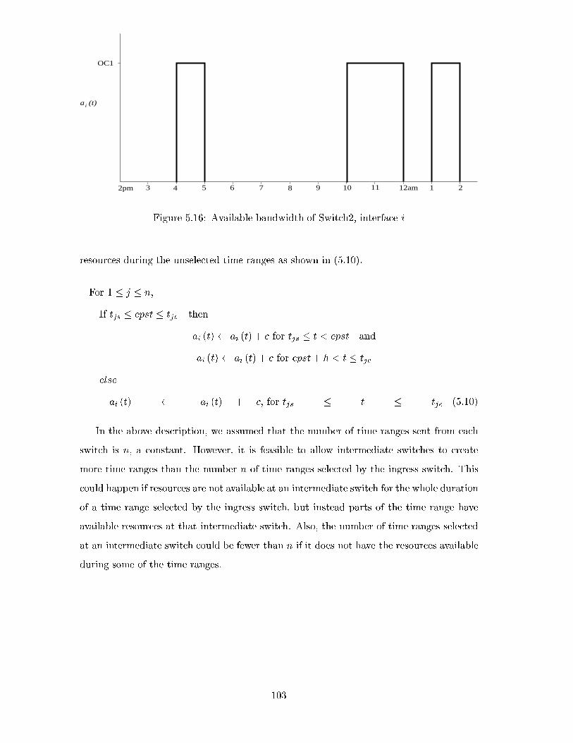
a (t)i
OC1
43 5 6 7 8 9 10 11 1 22pm 12am
Figure 5.16: Available bandwidth of Switch2, interface i
resources during the unselected time ranges as shown in (5.10).
For 1 � j � n;
If tjs � epst � tje then
ai (t) ai (t) + c for tjs � t < epst and
ai (t) ai (t) + c for epst+ h < t � tje
else
ai (t) ai (t) + c, for tjs � t � tje (5.10)
In the above description, we assumed that the number of time ranges sent from each
switch is n, a constant. However, it is feasible to allow intermediate switches to create
more time ranges than the number n of time ranges selected by the ingress switch. This
could happen if resources are not available at an intermediate switch for the whole duration
of a time range selected by the ingress switch, but instead parts of the time range have
available resources at that intermediate switch. Also, the number of time ranges selected
at an intermediate switch could be fewer than n if it does not have the resources available
during some of the time ranges.
103
5.6 Simulation and results
5.6.1 Network model
A comparison of the four di�erent connection setup schemes was done using simulation
with the help of the discrete event simulator OPNET Modeler [24]. The network model
studied is presented in Figure 5.17. It is a circuit-switched connection-oriented network
implementing a very simpli�ed CAC mechanism in which each channel is able to provide
one \bandwidth unit", which is requested by a connection. An analogy can be drawn
between this network and a SONET (Synchronous Optical NETwork) network in which
all the channels are OC1 channels. The network model consists of four switches and
all the links shown in Figure 5.17 are unidirectional channels providing one bandwidth
unit. In general networks will have much higher channel capacities. We chose only one
bandwidth unit for the interfaces to decrease the startup settling time of the simulations.
Connections were set up and released between Source and Dest, and between srcx and
destx. The connections between Source and Dest were studied (hence called study traÆc),
and the connections between srcx and destx were created as \interference traÆc" to create
a more realistic network model. Interarrival times of the connection setup requests and
the holding times of the connections are assumed to be exponentially distributed. The
destinations always accepted any connection, allowing us to concentrate on the CAC
performed by the switches.
The mean call interarrival time and mean holding time for the study traÆc was kept
constant through all the simulations while the mean call interarrival time and holding
times of the interference traÆc was varied. This allowed us to simulate the behaviour of
the di�erent connection setup schemes' under di�erent load conditions. The mean call
interarrival time used by Source was 25 seconds and the mean holding time was 5 seconds.
This computes to a mean load of 20% introduced to the network by Source.
Table 5.2 presents the combinations of mean holding time and mean interarrival time
used for the interference traÆc generated by src1, src2 and src3. During each simulation
run each of the sources generating interference traÆc did so using the same mean holding
time and mean interarrival time. With these di�erent load conditions, the OC1 channels
between switches will experience load varying from 25% to 95%, while the load on the
channel between Switch4 and Dest is kept constant at 20%.
Table 5.3 presents the parameters used for each scheduling scheme. There are no
parameters for the kTwait scheme. The parameter Dmax for the kTwait � Tmax scheme
104
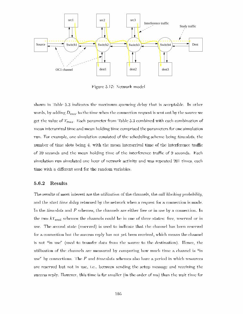
Switch1 Switch2 Switch3Source
src1
dest1
src2 src3
dest2
Switch4
dest3
Dest
Interference trafficStudy traffic
OC1 channel
Figure 5.17: Network model
shown in Table 5.3 indicates the maximum queueing delay that is acceptable. In other
words, by addingDmax to the time when the connection request is sent out by the source we
get the value of Tmax. Each parameter from Table 5.3 combined with each combination of
mean interarrival time and mean holding time comprised the parameters for one simulation
run. For example, one simulation consisted of the scheduling scheme being timeslots, the
number of time slots being 4, with the mean interarrival time of the interference traÆc
of 20 seconds and the mean holding time of the interference traÆc of 9 seconds. Each
simulation run simulated one hour of network activity and was repeated 201 times, each
time with a di�erent seed for the random variables.
5.6.2 Results
The results of most interest are the utilization of the channels, the call blocking probability,
and the start time delay returned by the network when a request for a connection is made.
In the timeslots and F schemes, the channels are either free or in use by a connection. In
the two kTwait schemes the channels could be in one of three states: free, reserved or in
use. The second state (reserved) is used to indicate that the channel has been reserved
for a connection but the success reply has not yet been received, which means the channel
is not \in use" (used to transfer data from the source to the destination). Hence, the
utilization of the channels are measured by computing how much time a channel is \in
use" by connections. The F and timeslots schemes also have a period in which resources
are reserved but not in use, i.e., between sending the setup message and receiving the
success reply. However, this time is far smaller (in the order of ms) than the wait time for
105
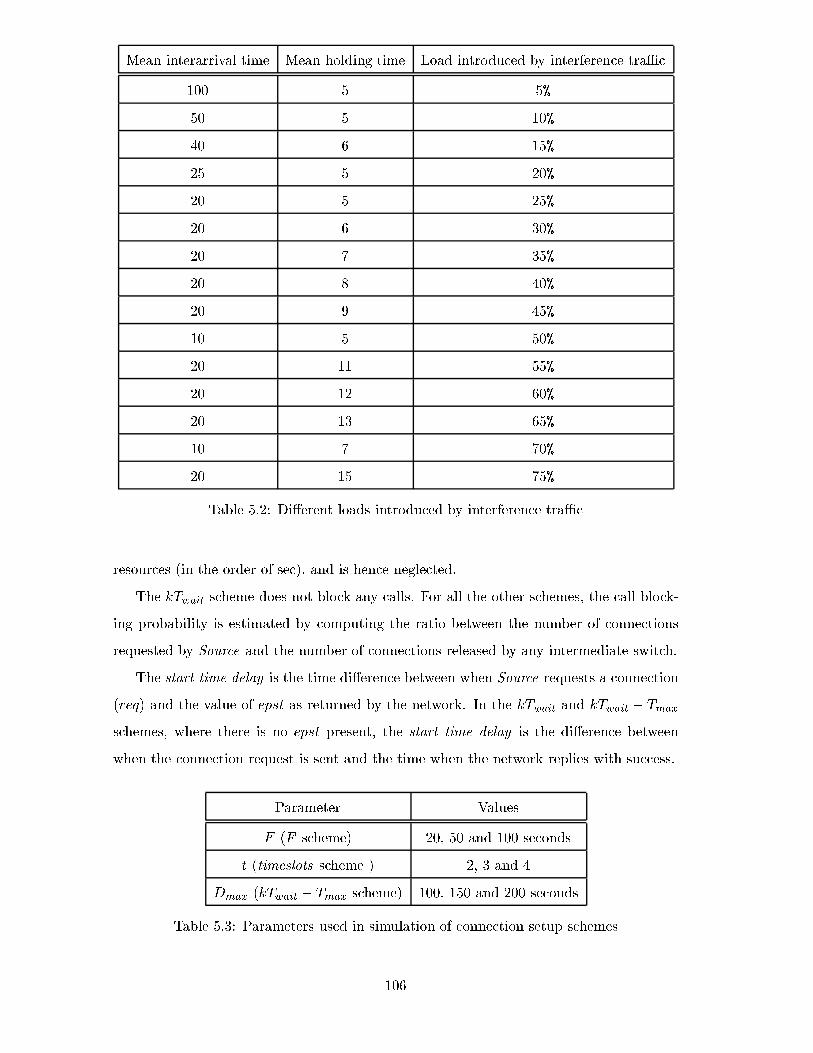
Mean interarrival time Mean holding time Load introduced by interference traÆc
100 5 5%
50 5 10%
40 6 15%
25 5 20%
20 5 25%
20 6 30%
20 7 35%
20 8 40%
20 9 45%
10 5 50%
20 11 55%
20 12 60%
20 13 65%
10 7 70%
20 15 75%
Table 5.2: Di�erent loads introduced by interference traÆc
resources (in the order of sec), and is hence neglected.
The kTwait scheme does not block any calls. For all the other schemes, the call block-
ing probability is estimated by computing the ratio between the number of connections
requested by Source and the number of connections released by any intermediate switch.
The start time delay is the time di�erence between when Source requests a connection
(req) and the value of epst as returned by the network. In the kTwait and kTwait � Tmax
schemes, where there is no epst present, the start time delay is the di�erence between
when the connection request is sent and the time when the network replies with success.
Parameter Values
F (F scheme) 20, 50 and 100 seconds
t (timeslots scheme ) 2, 3 and 4
Dmax (kTwait � Tmax scheme) 100, 150 and 200 seconds
Table 5.3: Parameters used in simulation of connection setup schemes
106

0
10
20
30
40
50
60
70
80
90
100
5/100 6/40 5/50 5/25 5/20 6/20 7/20 8/20 9/20 5/10 11/2012/2013/20 7/10 15/20
Bloc
ked
calls
(%)
mean holding time/mean interarrival time of "interference traffic"
F=20F=50
F=100t=2t=3t=4
Tmax=100Tmax=150Tmax=200
Figure 5.18: Percentage of calls blocked using di�erent connection setup schemes
Figure 5.18 shows the percentage of calls blocked when each connection setup scheme
is used. The kTwait � Tmax scheme performs the worst, even with the usage of a Dmax
value of 200 seconds the blocking percentage is almost 90%. The reason for this high
blocking rate can be explained by looking at the queue at Switch1 in which connection
requests requiring access to the channel that connects Switch1 to Switch2 are placed.
With an increase in interference traÆc, this queue grows very large and causes connection
requests to experience delays larger than the Dmax value used, causing the connection
to be blocked. Due to the poor performance of the kTwait � Tmax scheme (as shown in
Fig. 5.20) we dismiss it from further comparisons.
The call blocking percentages of the F scheme proves that increasing the value of F
decreases the call blocking probability signi�cantly. With the usage of a large F value
by Switch1, the chances that a succeeding switch can admit a call during the same time
Switch1 is able to admit it increases signi�cantly. Using a small F value (for example 20
seconds) when the average call holding time is large (13 or 15 seconds) serves to increase
call blocking.
Increasing the number of time ranges used by the timeslots scheme decreases blocking
probability signi�cantly. Increasing the number of time ranges selected by the ingress
switch improves the chances that an intermediate switch will �nd an overlapping time
107
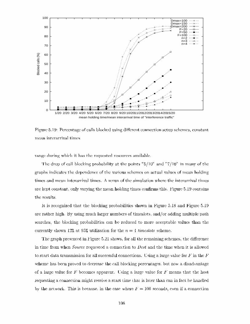
0
10
20
30
40
50
60
70
80
90
100
1/20 2/20 3/20 4/20 5/20 6/20 7/20 8/20 9/20 10/2011/2012/2013/2014/2015/20
Bloc
ked
calls
(%)
mean holding time/mean interarrival time of "interference traffic"
Dmax=100Dmax=150Dmax=200
F=20F=50
F=100n=2n=3n=4
Figure 5.19: Percentage of calls blocked using di�erent connection setup schemes, constant
mean interarrival times
range during which it has the requested resources available.
The drop of call blocking probability at the points "5/10" and "7/10" in many of the
graphs indicates the dependence of the various schemes on actual values of mean holding
times and mean interarrival times. A rerun of the simulation where the interarrival times
are kept constant, only varying the mean holding times con�rms this. Figure 5.19 contains
the results.
It is recognized that the blocking probabilities shown in Figure 5.18 and Figure 5.19
are rather high. By using much larger numbers of timeslots, and/or adding multiple path
searches, the blocking probabilities can be reduced to more acceptable values than the
currently shown 12% at 95% utilization for the n = 4 timeslots scheme.
The graph presented in Figure 5.21 shows, for all the remaining schemes, the di�erence
in time from when Source requested a connection to Dest and the time when it is allowed
to start data transmission for all successful connections. Using a large value for F in the F
scheme has been proved to decrease the call blocking percentages, but now a disadvantage
of a large value for F becomes apparent. Using a large value for F means that the host
requesting a connection might receive a start time that is later than can in fact be handled
by the network. This is because, in the case where F = 100 seconds, even if a connection
108
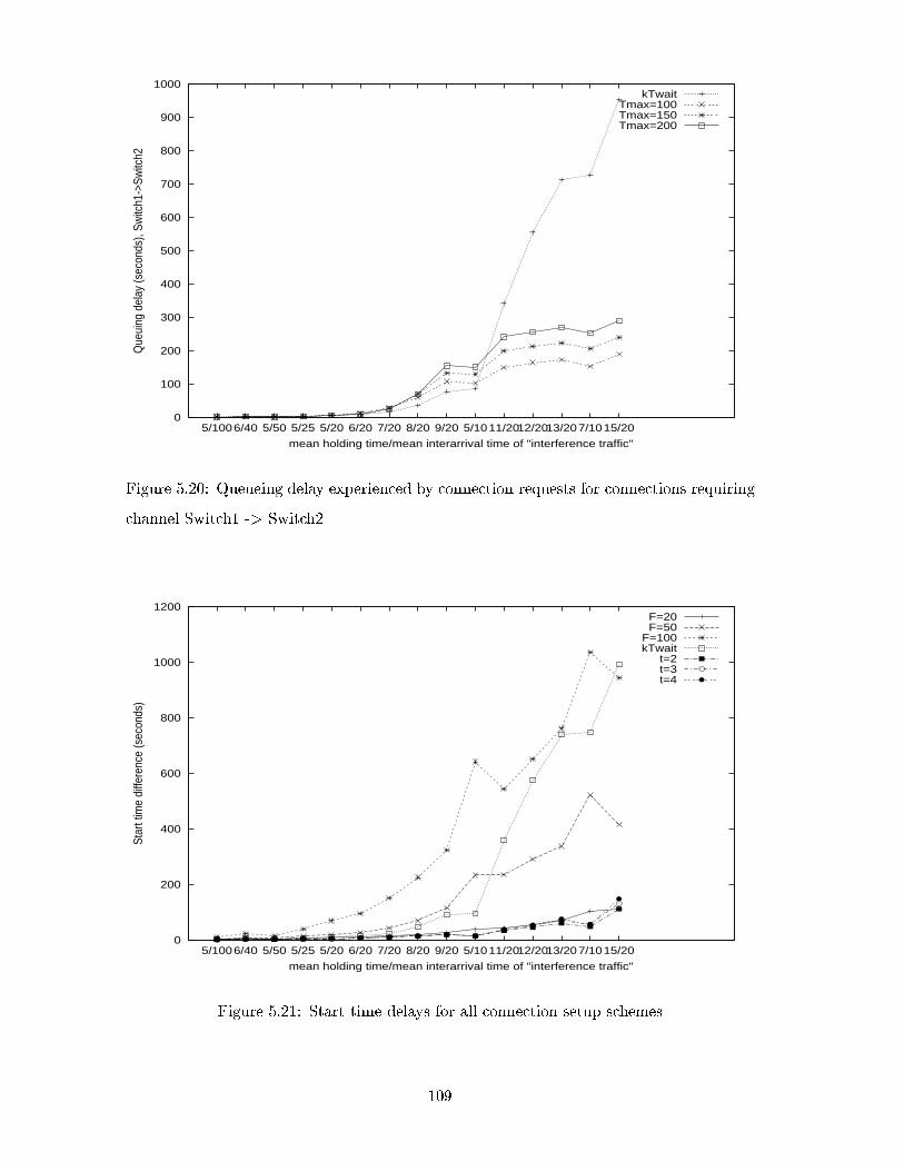
0
100
200
300
400
500
600
700
800
900
1000
5/1006/40 5/50 5/25 5/20 6/20 7/20 8/20 9/20 5/1011/2012/2013/207/1015/20
Que
uing
del
ay (s
econ
ds),
Switc
h1->
Switc
h2
mean holding time/mean interarrival time of "interference traffic"
kTwaitTmax=100Tmax=150Tmax=200
Figure 5.20: Queueing delay experienced by connection requests for connections requiring
channel Switch1 -> Switch2
0
200
400
600
800
1000
1200
5/1006/40 5/50 5/25 5/20 6/20 7/20 8/20 9/20 5/1011/2012/2013/207/1015/20
Star
t tim
e di
ffere
nce
(sec
onds
)
mean holding time/mean interarrival time of "interference traffic"
F=20F=50
F=100kTwait
t=2t=3t=4
Figure 5.21: Start time delays for all connection setup schemes
109
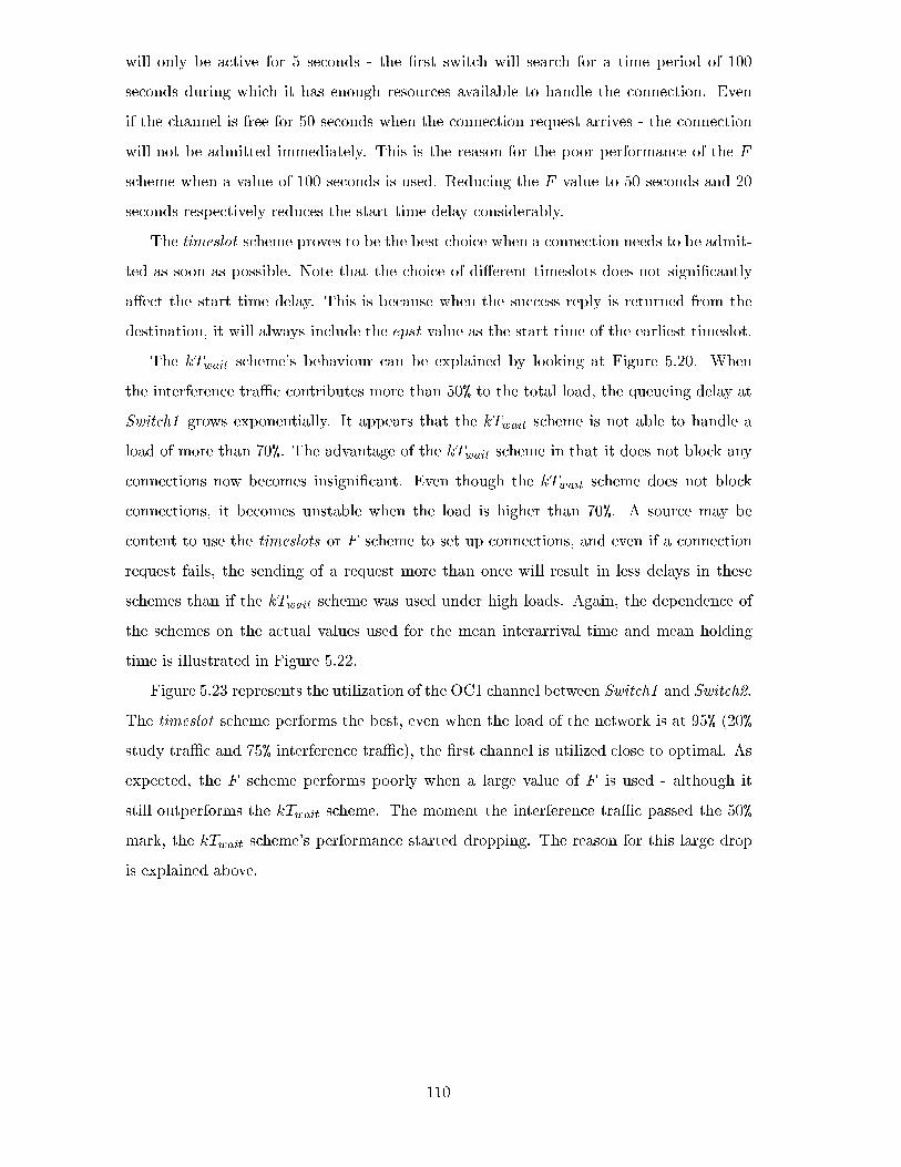
will only be active for 5 seconds - the �rst switch will search for a time period of 100
seconds during which it has enough resources available to handle the connection. Even
if the channel is free for 50 seconds when the connection request arrives - the connection
will not be admitted immediately. This is the reason for the poor performance of the F
scheme when a value of 100 seconds is used. Reducing the F value to 50 seconds and 20
seconds respectively reduces the start time delay considerably.
The timeslot scheme proves to be the best choice when a connection needs to be admit-
ted as soon as possible. Note that the choice of di�erent timeslots does not signi�cantly
a�ect the start time delay. This is because when the success reply is returned from the
destination, it will always include the epst value as the start time of the earliest timeslot.
The kTwait scheme's behaviour can be explained by looking at Figure 5.20. When
the interference traÆc contributes more than 50% to the total load, the queueing delay at
Switch1 grows exponentially. It appears that the kTwait scheme is not able to handle a
load of more than 70%. The advantage of the kTwait scheme in that it does not block any
connections now becomes insigni�cant. Even though the kTwait scheme does not block
connections, it becomes unstable when the load is higher than 70%. A source may be
content to use the timeslots or F scheme to set up connections, and even if a connection
request fails, the sending of a request more than once will result in less delays in these
schemes than if the kTwait scheme was used under high loads. Again, the dependence of
the schemes on the actual values used for the mean interarrival time and mean holding
time is illustrated in Figure 5.22.
Figure 5.23 represents the utilization of the OC1 channel between Switch1 and Switch2.
The timeslot scheme performs the best, even when the load of the network is at 95% (20%
study traÆc and 75% interference traÆc), the �rst channel is utilized close to optimal. As
expected, the F scheme performs poorly when a large value of F is used - although it
still outperforms the kTwait scheme. The moment the interference traÆc passed the 50%
mark, the kTwait scheme's performance started dropping. The reason for this large drop
is explained above.
110
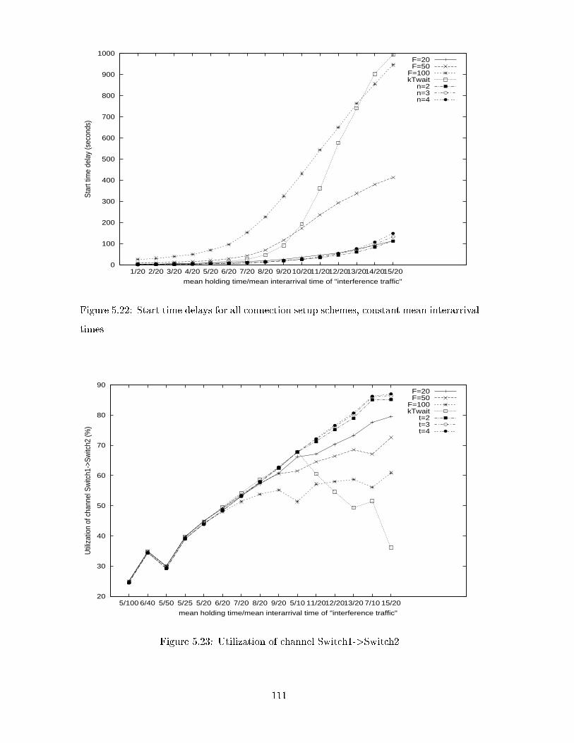
0
100
200
300
400
500
600
700
800
900
1000
1/20 2/20 3/20 4/20 5/20 6/20 7/20 8/20 9/2010/2011/2012/2013/2014/2015/20
Star
t tim
e de
lay
(sec
onds
)
mean holding time/mean interarrival time of "interference traffic"
F=20F=50
F=100kTwait
n=2n=3n=4
Figure 5.22: Start time delays for all connection setup schemes, constant mean interarrival
times
20
30
40
50
60
70
80
90
5/100 6/40 5/50 5/25 5/20 6/20 7/20 8/20 9/20 5/10 11/2012/2013/20 7/10 15/20
Util
izat
ion
of c
hann
el S
witc
h1->
Switc
h2 (%
)
mean holding time/mean interarrival time of "interference traffic"
F=20F=50
F=100kTwait
t=2t=3t=4
Figure 5.23: Utilization of channel Switch1->Switch2
111
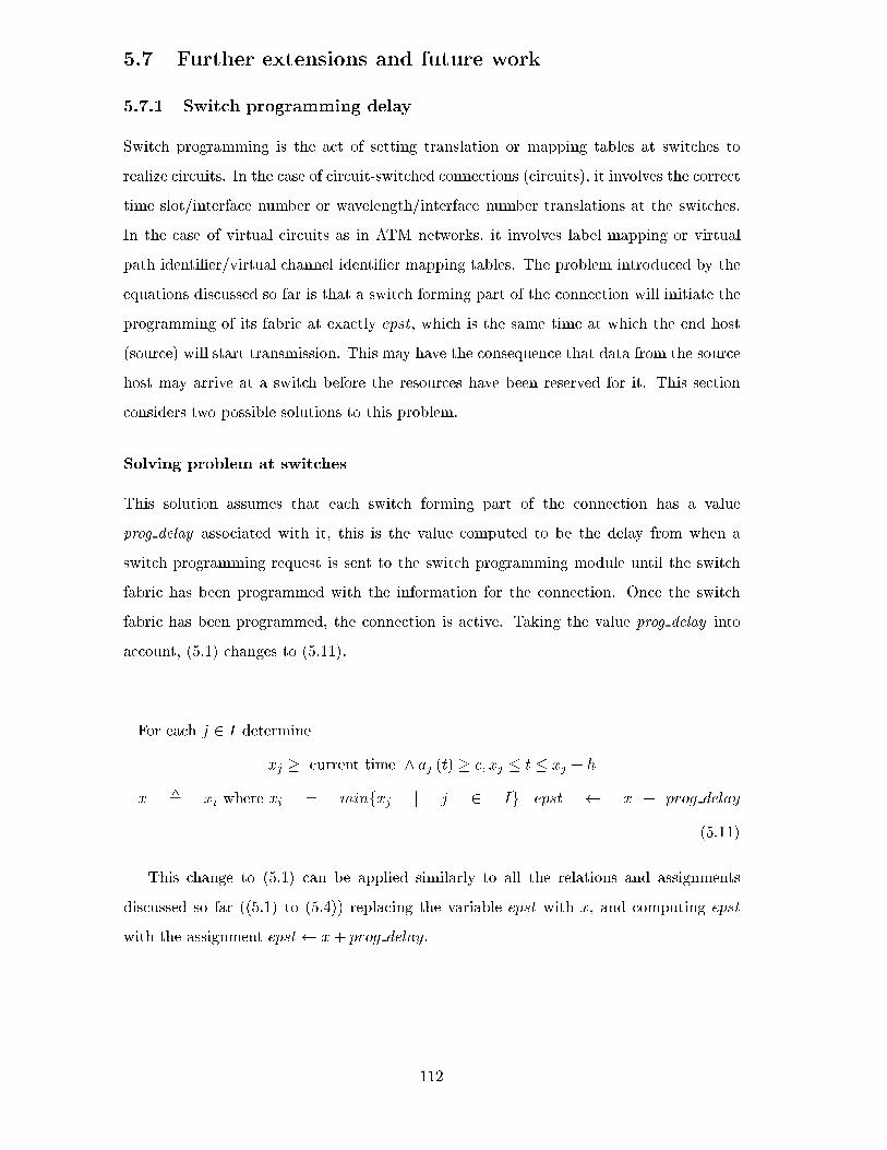
5.7 Further extensions and future work
5.7.1 Switch programming delay
Switch programming is the act of setting translation or mapping tables at switches to
realize circuits. In the case of circuit-switched connections (circuits), it involves the correct
time slot/interface number or wavelength/interface number translations at the switches.
In the case of virtual circuits as in ATM networks, it involves label mapping or virtual
path identi�er/virtual channel identi�er mapping tables. The problem introduced by the
equations discussed so far is that a switch forming part of the connection will initiate the
programming of its fabric at exactly epst, which is the same time at which the end host
(source) will start transmission. This may have the consequence that data from the source
host may arrive at a switch before the resources have been reserved for it. This section
considers two possible solutions to this problem.
Solving problem at switches
This solution assumes that each switch forming part of the connection has a value
prog delay associated with it, this is the value computed to be the delay from when a
switch programming request is sent to the switch programming module until the switch
fabric has been programmed with the information for the connection. Once the switch
fabric has been programmed, the connection is active. Taking the value prog delay into
account, (5.1) changes to (5.11).
For each j 2 I determine
xj � current time ^ aj (t) � c; xj � t � xj + h
x , xi where xi = minfxj j j 2 Ig epst x + prog delay
(5.11)
This change to (5.1) can be applied similarly to all the relations and assignments
discussed so far ((5.1) to (5.4)) replacing the variable epst with x, and computing epst
with the assignment epst x+ prog delay.
112
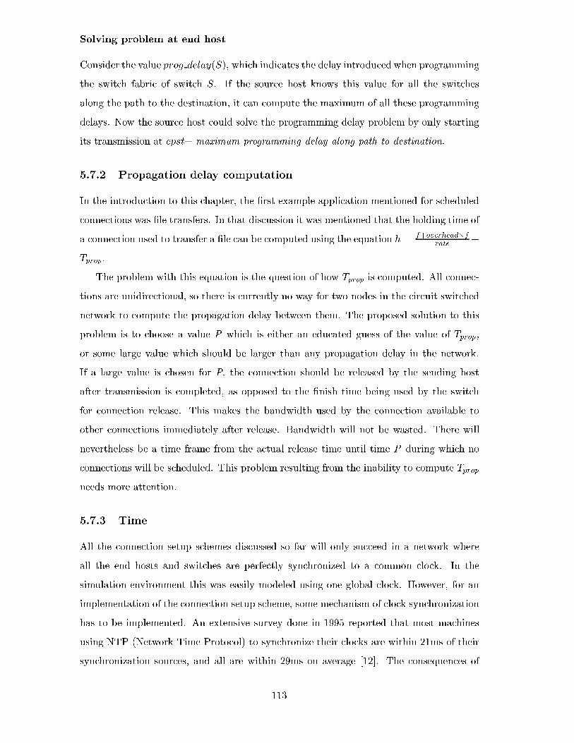
Solving problem at end host
Consider the value prog delay(S), which indicates the delay introduced when programming
the switch fabric of switch S. If the source host knows this value for all the switches
along the path to the destination, it can compute the maximum of all these programming
delays. Now the source host could solve the programming delay problem by only starting
its transmission at epst+ maximum programming delay along path to destination.
5.7.2 Propagation delay computation
In the introduction to this chapter, the �rst example application mentioned for scheduled
connections was �le transfers. In that discussion it was mentioned that the holding time of
a connection used to transfer a �le can be computed using the equation h = f+overhead�frate
+
Tprop.
The problem with this equation is the question of how Tprop is computed. All connec-
tions are unidirectional, so there is currently no way for two nodes in the circuit switched
network to compute the propagation delay between them. The proposed solution to this
problem is to choose a value P which is either an educated guess of the value of Tprop,
or some large value which should be larger than any propagation delay in the network.
If a large value is chosen for P, the connection should be released by the sending host
after transmission is completed, as opposed to the �nish time being used by the switch
for connection release. This makes the bandwidth used by the connection available to
other connections immediately after release. Bandwidth will not be wasted. There will
nevertheless be a time frame from the actual release time until time P during which no
connections will be scheduled. This problem resulting from the inability to compute Tprop
needs more attention.
5.7.3 Time
All the connection setup schemes discussed so far will only succeed in a network where
all the end hosts and switches are perfectly synchronized to a common clock. In the
simulation environment this was easily modeled using one global clock. However, for an
implementation of the connection setup scheme, some mechanism of clock synchronization
has to be implemented. An extensive survey done in 1995 reported that most machines
using NTP (Network Time Protocol) to synchronize their clocks are within 21ms of their
synchronization sources, and all are within 29ms on average [12]. The consequences of
113
di�erent times at switches have not been examined, but it is expected that the scheduling
mechanisms will not perform well in such an environment. This is because situations may
arise when data is received before a connection is set up, or a connection is closed before
data transmission is completed. Mechanisms that use relative time values or some such
approach are needed to deal with these time di�erences.
5.8 Summary and Conclusions
This chapter described various scheduling algorithms for calls with known holding times.
To support multiple-switch connections, two scheduling alternatives, the F scheme and
timeslots scheme, were proposed. In the F scheme, resources are reserved for a long
period F , longer than the call holding time, to guarantee that all switches would �nd a
start time for the connection within this long period. In the timeslots scheme, multiple
time ranges when the ingress switch can support the call are selected and sent downstream
in the signaling message. Each intermediate switch then selects a subset from within this
set, until the destination is reached. These two schemes were compared against a simple
call queueing scheme, the kTwait scheme, which does not assume knowledge of call holding
times, and a variant of this scheme. A simulation study of the schemes showed that
(a) signi�cant gains are possible by using knowledge of known call holding times, if that
is available, and (b) of the two alternatives proposed for scheduling calls with known
holding times, the timeslots scheme proved to be the better alternative. The kTwait
scheme becomes unstable when the traÆc load exceeds 70%. At 70% loading, the timeslots
algorithm that uses knowledge of holding times can o�er start time delays that are 85%
smaller than with the kTwait that does not assume knowledge of call holding times. Also,
the timeslots scheme can be used with traÆc loads of 95%. As a result, at 70% load a
channel utilization increase of 37% is possible using schemes that exploit knowledge of call
holding times, when compared to the kTwait scheme. The reason we consider the timeslots
scheme the winner over the F scheme, is that at large values of F , call blocking is low,
but the start time delay is high, and with small values of F , the inverse is true. On the
other hand, in the timeslots scheme, both the call blocking probability and the start time
delay are relatively low for all loads tested. Its drawback over the F scheme lies in the
increased signaling overhead, which might be negligible if few time slots are used.
The novelty of this work lies in its introduction of call queueing and providing delayed
starts for connections. It culminates in a proposal to use known call holding times while
114

scheduling to improve both network resource utilization and call queueing delays.
115
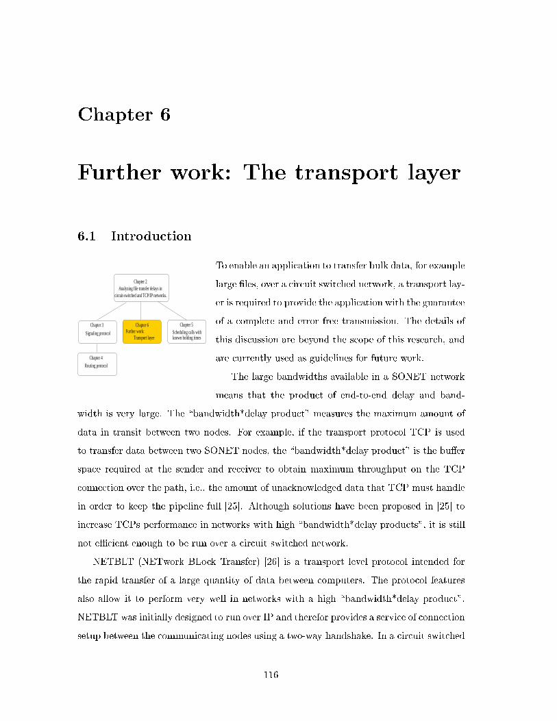
Chapter 6
Further work: The transport layer
6.1 Introduction
Chapter 2Analyzing file transfer delays in
circuit-switched and TCP/IP networks.
Chapter 6Further work:
Transport layer
Chapter 3
Signaling protocol
Chapter 5Scheduling calls with known holding times
Chapter 4
Routing protocol
To enable an application to transfer bulk data, for example
large �les, over a circuit switched network, a transport lay-
er is required to provide the application with the guarantee
of a complete and error free transmission. The details of
this discussion are beyond the scope of this research, and
are currently used as guidelines for future work.
The large bandwidths available in a SONET network
means that the product of end-to-end delay and band-
width is very large. The \bandwidth*delay product" measures the maximum amount of
data in transit between two nodes. For example, if the transport protocol TCP is used
to transfer data between two SONET nodes, the \bandwidth*delay product" is the bu�er
space required at the sender and receiver to obtain maximum throughput on the TCP
connection over the path, i.e., the amount of unacknowledged data that TCP must handle
in order to keep the pipeline full [25]. Although solutions have been proposed in [25] to
increase TCPs performance in networks with high \bandwidth*delay products", it is still
not eÆcient enough to be run over a circuit switched network.
NETBLT (NETwork BLock Transfer) [26] is a transport level protocol intended for
the rapid transfer of a large quantity of data between computers. The protocol features
also allow it to perform very well in networks with a high \bandwidth*delay product".
NETBLT was initially designed to run over IP and therefor provides a service of connection
setup between the communicating nodes using a two-way handshake. In a circuit switched
116
network, the transport layer does not need to set up a connection between the transport
entities due to the fact that a (network layer) connection has already been set up between
the communicating nodes.
Instead of examining more transport protocols to �nd an ideal protocol to be used
for �le transfers in a circuit switched network, the functions of transport protocols are
examined. Section 6.2 brie y discusses the transport layer capabilities that are envisioned
to be ideal when a circuit switched network is used to transfer bulk data. These capabilities
are currently being evaluated by the CATT research group for the design of a new transport
protocol.
6.2 Protocol requirements
The transport protocol is responsible for guaranteeing a reliable data transport service
between two nodes connected with a uni-directional (from the source to the destination)
channel. A uni-directional link limits the communication between the two transport enti-
ties, but creating a bi-directional link between the transport entities will result in a waste
of bandwidth. For example, the smallest channel available in a SONET network is OC1
(51.84Mbps), which, when dedicated to communication between transport entities for the
whole duration of a �le transfer, will be very wasteful. Recall that all the nodes forming
part of the SONET network will have interfaces connecting them to the IP network. It is
therefore proposed that all messages from the destination transport entity to the source
transport entity be sent over an IP network. These messages are few during a �le transfer.
They should not add an excessive load to the IP network.
Figure 6.1 shows the paths TPDUs (Transport Protocol Data Units) will follow between
two nodes connected by a network layer connection.
The services provided by a transport protocol are:
� connection management, which is a mechanism needed to maintain state information
regarding the data transfer at the source and destination;
� ow control to avoid bu�er over ows at the destination;
� acknowledgements received by the source that indicate the reception of data (suc-
cessful or unsuccessful) by the destination;
� error handling that includes error detection and recovery schemes;
117
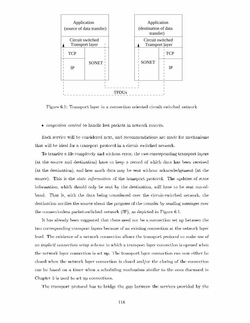
Application(source of data transfer)
Application(destination of data
transfer)
TPDUs
Transport layerCircuit switched
TCP
SONET SONET
TCP
IPIP
Circuit switchedTransport layer
Figure 6.1: Transport layer in a connection oriented circuit switched network
� congestion control to handle lost packets in network routers.
Each service will be considered next, and recommendations are made for mechanisms
that will be ideal for a transport protocol in a circuit switched network.
To transfer a �le completely and without error, the two corresponding transport layers
(at the source and destination) have to keep a record of which data has been received
(at the destination), and how much data may be sent without acknowledgement (at the
source). This is the state information of the transport protocol. The updates of state
information, which should only be sent by the destination, will have to be sent out-of-
band. That is, with the data being transferred over the circuit-switched network, the
destination noti�es the source about the progress of the transfer by sending messages over
the connectionless packet-switched network (IP), as depicted in Figure 6.1.
It has already been suggested that there need not be a connection set up between the
two corresponding transport layers because of an existing connection at the network layer
level. The existence of a network connection allows the transport protocol to make use of
an implicit connection setup scheme in which a transport layer connection is opened when
the network layer connection is set up. The transport layer connection can now either be
closed when the network layer connection is closed and/or the closing of the connection
can be based on a timer when a scheduling mechanism similar to the ones discussed in
Chapter 5 is used to set up connections.
The transport protocol has to bridge the gap between the services provided by the
118
network layer, and the services required by higher layers [27]. In our target application
of �le transfer over a circuit switched network, it is assumed that when the (transport
layer) connection is set up, the applications would already have agreed on the transfer
rate acceptable to both the source and destination, which has been negotiated during
the setup of the network layer connection. The decision to use an implicit transport
layer connection setup scheme implies that all transport layer parameters that need to be
negotiated are agreed to during network layer connection setup.
The rate at which the destination can accept data is taken into account when the
circuit is set up. Because a circuit-switched network is used to transfer the data, the
network will never become congested due to the reservation of resources in the network.
But, once a connection is set up between the network layers of the source and destination,
it is possible that, (due to variations in host tasks activity) the destination might not
be able to accept data at the rate it had been able to handle when the network layer
connection was set up. Thus, some ow control mechanism needs to be introduced to
enable the destination to notify the source that it needs to limit the data transmission.
For ow control, the mechanism of rate control is ideal. Using rate control the destination
can ask the source to send data at a lower rate. For example, if an OC12 connection has
been set up between the source and destination, the destination can request the source to
send data at OC1 rate. This has the consequence that some resources might be wasted in
the circuit-switched network during the times that the destination is not able to handle
the initial data rate.
Data being transferred over a circuit-switched network will never be delivered out of
sequence. This leaves the transport protocol with two responsibilities. First, all the data
sent by the source has to reach the destination application free of bit errors (error free de-
livery). Second, all data transmitted by the source has to reach the destination (complete
delivery). The usage of sequence numbers is required for error correction. Byte-based
sequence numbers (as used in TCP) allows for eÆcient error correction by indicating the
exact amount of data that is missing or containing errors, but considering the amount
of bytes that could be in transit between two nodes in a SONET network, the sequence
numbers will get really large. Thus a packet based sequence numbering scheme is pro-
posed. Because the TPDUs will always arrive in sequence, a missing packet will be easily
discovered. The destination can request the retransmission of a missing packet by sending
a NAK (Negative Acknowledgement) to the source on the IP network. By making use of
119

NAKs, as opposed to positive acknowledgements (ACKs) only used for data received error
free and in sequence, the signaling load is reduced considerably.
Additionally each TPDU could include a FEC (Forward Error Correction) code that
is able to handle the most frequently occurring error patterns. When an error is encoun-
tered in a TPDU, a NAK is sent to the source requesting a retransmission of the packet
(identi�ed by its sequence number), similarly to the mechanism summarized in [28].
To determine if all the data transmitted by the source has reached the destination
(complete delivery), it is proposed that all TPDUs are always the same length, except
possibly the last TPDU. The last TPDU also includes an indication to report that it is
the last TPDU of the transmission, thus indicating a complete transmission. Once the
transport protocol receives this indication, it can signal the SONET signaling process to
close the network layer connection. Given that circuits are best used with continuous
traÆc (rather than bursty), our thinking is that it is appropriate to disconnect the circuit
when transmission is done.
6.3 Conclusion
Only a few design decisions have been considered for the transport protocol. The decisions
should result in a light-weight transport protocol that allows for the complete and error
free data delivery in a circuit switched network. The interfaces between the transport
layer and the network and application layers still needs to be de�ned, as well as the detail
of all the mechanisms described above.
120
Chapter 7
Conclusion
This research set out to �nd eÆcient mechanisms for bulk data transfer. An analytical
and experimental analysis of �le transfer delay in circuit-switched and TCP/IP networks
suggested that circuit-switching is ideally suited for bulk data transfer.
To enable TDM networks to be used for bulk data transfer, a mechanism is required
to enable the setting up of high-bandwidth on-demand circuits. This is because switched
connections (as opposed to provisioned connections) are currently only available at the
low rate of DS0(64Kbps) while data rates of OC1(51.84Mbps) to OC768(40Gbps) would
be ideal for bulk data transfer. A signaling and supporting routing protocol that enables
on demand setup of circuits with rates of OC1 to OC192 was designed to reach this
goal. For high throughput and a general increase in eÆciency, the signaling protocol was
designed to be implemented in hardware, and the routing tables used by it are updated
by a routing protocol that was designed to be implemented in software. The signaling
protocol is currently being implemented in hardware by the CATT research group.
Bulk data has the characteristic that when it is transferred over a connection-oriented
network that implements preventative congestion control mechanisms (as opposed to re-
active congestion control as implemented in TCP/IP networks), the duration or holding
time of the connection can be determined by using the �lesize, data rate and propagation
delays.
Two scheduling algorithms were designed that use these known holding times. These
algorithms enable a switch to reply with a later start time if it is unable to accommodate
the connection request at the time of its arrival. The scheduling algorithms are simulated
and compared to a simple queueing mechanism where a connection request is queued until
its requested resources become available, only then being forwarded to the next hop of the
121
connection.
The use of such scheduling is shown to improve the eÆciency of bulk data transfer in
connection-oriented networks. The simulations show that at 70% loading, these schemes
o�er start time delays that are up to 85% smaller and channel utilization of up to 37%
larger than a simple queueing mode of operation where call holding times are ignored
when connections are set up.
The evidence thus suggests that with appropriate signaling and scheduling, eÆcient
bulk data transfer can be achieved on circuit-switched networks. Of course, a suitable
transport protocol would be required to enable the reliable transfer of data between two
hosts. While the ideal characteristics of such a protocol have been described in this
dissertation, details of its design and implementation remain a matter for future research.
122

Bibliography
[1] Lawrence Berkeley National Laboratory Network Research Group, \Tcpdump ver.
3.4", ftp://ftp.ee.lbl.gov/tcpdump.tar.Z
[2] D. Niehaus, A. Battou, A. McFarland, B. Decina, H. Dardy, V. Sirkay, B. Edwards,
\Performance Benchmarking of Signaling in ATM Networks," IEEE Communications
Magazine, August 1997, pp. 134-143.
[3] H Ren-Hung, J. F. Kurose, D. Towsley, \On Call-Processing Delay in High Speed
Networks," IEEE/ACM Trans. on Networking, Vol. 3, No. 6, December 1995, pp.
628-639.
[4] Gmsli Hjalmtsson and K. K. Ramakrishnan, \UNITE - An Architecture for
Lightweight Signaling in ATM Networks," in Proceedings of IEEE Infocom'98, San
Francisco, CA.
[5] Mischa Schwartz, \Telecommunication Networks," Addison-Wesley Publishing Com-
pany, 1988.
[6] Editor: John C. McDonald, \Fundamentals of Digital Switching," Plenum Press,
1983.
[7] H. Miyahara, T. Hasegawa, and Y. Teshigawara, \A Comparative Evaluation of
Switching Methods in Computer Communication Networks," IEEE ICC, San Fran-
cisco, pp. 6-6-6-10, June 1975.
[8] T. V. Lakshman and D. Stiliadis,\High-speed policy-based packet forwarding using
eÆcient multi-dimensional range matching," Proceedings of ACM SIGCOMM'98, pp.
203-214.
[9] \Private Network-Network Interface Speci�cation Version 1.0, " The ATM Forum.
123
[10] \ Internet Protocol, DARPA Internet program, Protocol speci�cation", RFC 791,
September 1981.
[11] Editor: R. Braden, \Requirements for Internet Hosts { Communication Layers", RFC
1122, October 1989.
[12] David L. Mills, Ajit Thyagarjan and Brian C. Hu�man, \Internet timekeeping around
the globe," Proc. Precision Time and Time Interval (PTTI) Applications and Plan-
ning Meeting, Long Beach CA, December 1997.
[13] ITU-T Recommendation Q.850, \ Usage of Cause and Location in the Digital Sub-
scriber Signalling System No. 1 and the Signalling System No. 7 ISDN User Part".
[14] ITU-T Recommendation Q.2931, \B-ISDN DSS2 User-Network Interface (UNI) Layer
3 Speci�cations for Basic Call/Connection Control."
[15] K. Thompson, G.J. Miller and R. Wilder, \Wide-Area Internet TraÆc Patterns and
Characteristics," IEEE Network November/December 1997, pp.10-23.
[16] Marcel Waldvogel, G. Varghese, J. Turner, B. Plattner, \Scalable High-Speed IP
Routing Lookups," Proceedings of ACM SIGCOMM, Sep. 1997.
[17] P. Gupta, S. Lin and N. Mckeown, \Routing Lookups in Hardware at Memory Access
Speeds," Proceedings of IEEE INFOCOM 1998.
[18] A. McAuley and P. Francis, \Fast Routing Table Lookup using CAMs," Proceedings
of IEEE INFOCOM, pp. 1382-1391, 1993.
[19] J. Moy, \OSPF Version 2," RFC 2328, April 1998.
[20] C. Hedrick, \Routing Information Protocol, " RFC 1058, June 1988.
[21] J. Postel, \Assigned numbers, " RFC 790, September 1981.
[22] \Stream Control Transmission Protocol," Internet-Draft, April 2000 expires October
2000.
[23] \http://metalab.unc.edu/pub/Linux/MIRRORS.html", accessed 20 March 2000
[24] Opnet Technologies, Inc., \OPNET modeler,"
http://www.opnet.com/products/modeler/home.html.
124
[25] V. Jacobson, R. Braden and D. Borman, \TCP extensions for high performance,"
RFC1323, May 1992.
[26] D.D. Clark, M.L. Lambert and L. Zhang, \NETBLT: A bulk data transfer protocol,"
RFC998, March 1987.
[27] W.A. Doeringer, D. Dykeman, M. Kaiserswerth, B.W. Meister, H. Rudin and R.
Williamson, \A survey of light-weight transport protocols for high-speed networks,"
IEEE transactions on communications, vol. 38, no. 11, pp.2025-2039, November 1990.
[28] D.J. Costello, J. Hagenauer, H. Imai and S.B. Wicker, \Applications of error-control
coding," IEEE transactions on information theory, vol. 44, no. 6, pp.2531-2560, Oc-
tober 1998.
125