Signals and Systems: IntroductionCEN340: Signals and Systems; Ghulam Muhammad 18 1.2 Transformations of the Independent Variable The transformationofasignalis one of the central concepts

Signals and Systems: Introduction

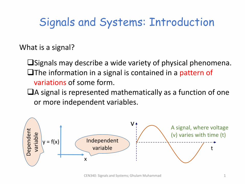
What is a signal?

Signals may describe a wide variety of physical phenomena.The information in a signal is contained in a pattern of

variations of some form.A signal is represented mathematically as a function of one

or more independent variables.

x

y = f(x) Independent variable

Dep

en

den

t va

riab

le

t

vA signal, where voltage (v) varies with time (t)

CEN340: Signals and Systems; Ghulam Muhammad 1

0 100 200 300 400-1

-0.5

0

0.5

1

Time (ms)

Am

plit

ud

e

Time (ms)

Am

plit

ud

e, m

V

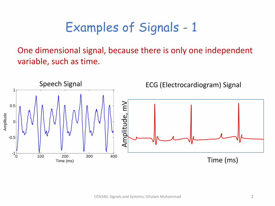
Examples of Signals - 1


Speech Signal ECG (Electrocardiogram) Signal

One dimensional signal, because there is only one independent variable, such as time.


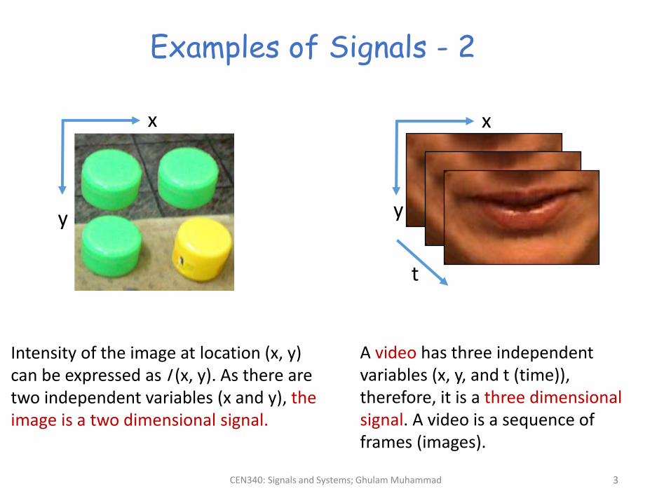
Examples of Signals - 2

x

y

Intensity of the image at location (x, y) can be expressed as I (x, y). As there are two independent variables (x and y), the image is a two dimensional signal.

x

y

t

A video has three independent variables (x, y, and t (time)), therefore, it is a three dimensional signal. A video is a sequence of frames (images).


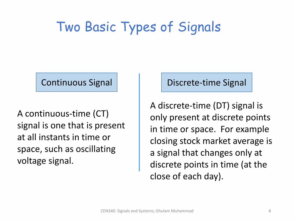
Two Basic Types of Signals

Continuous Signal Discrete-time Signal

A continuous-time (CT) signal is one that is present at all instants in time or space, such as oscillating voltage signal.

A discrete-time (DT) signal is only present at discrete points in time or space. For example closing stock market average is a signal that changes only at discrete points in time (at the close of each day).

Continuous time

Co

nti

nu

ou

s am

plit

ud

e

Discrete time

Co

nti

nu

ou

s am

plit

ud

e

Discrete time

Dis

cret

e am

plit

ud

e

Continuous Signal

Discrete-time Signal

Digital Signal


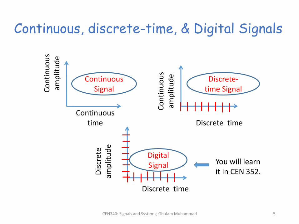
Continuous, discrete-time, & Digital Signals

You will learn it in CEN 352.


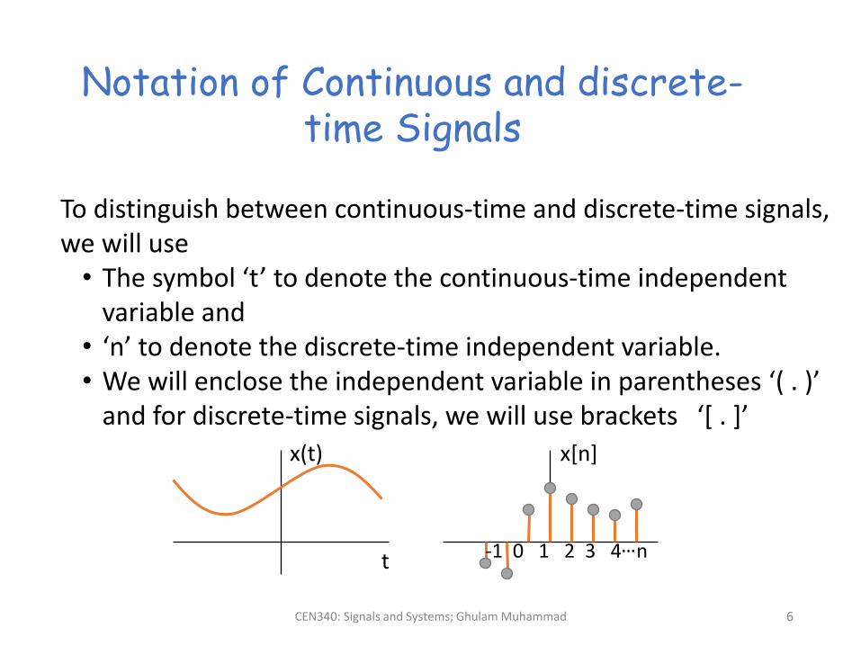
Notation of Continuous and discrete-time Signals

To distinguish between continuous-time and discrete-time signals, we will use• The symbol ‘t’ to denote the continuous-time independent

variable and• ‘n’ to denote the discrete-time independent variable.• We will enclose the independent variable in parentheses ‘( . )’

and for discrete-time signals, we will use brackets ‘[ . ]’

x(t) x[n]

t -1 0 1 2 3 4 n…


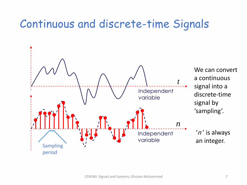
Continuous and discrete-time Signals

tIndependent

variable

Independent

variable

n

Sampling period

We can convert a continuous signal into a discrete-time signal by ‘sampling’.

‘n ’ is always an integer.


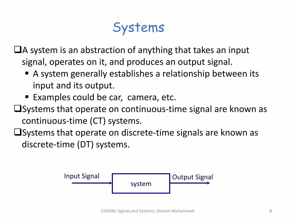
A system is an abstraction of anything that takes an input signal, operates on it, and produces an output signal. A system generally establishes a relationship between its

input and its output. Examples could be car, camera, etc.

Systems that operate on continuous-time signal are known as continuous-time (CT) systems.

Systems that operate on discrete-time signals are known as discrete-time (DT) systems.

Systems

systemInput Signal Output Signal


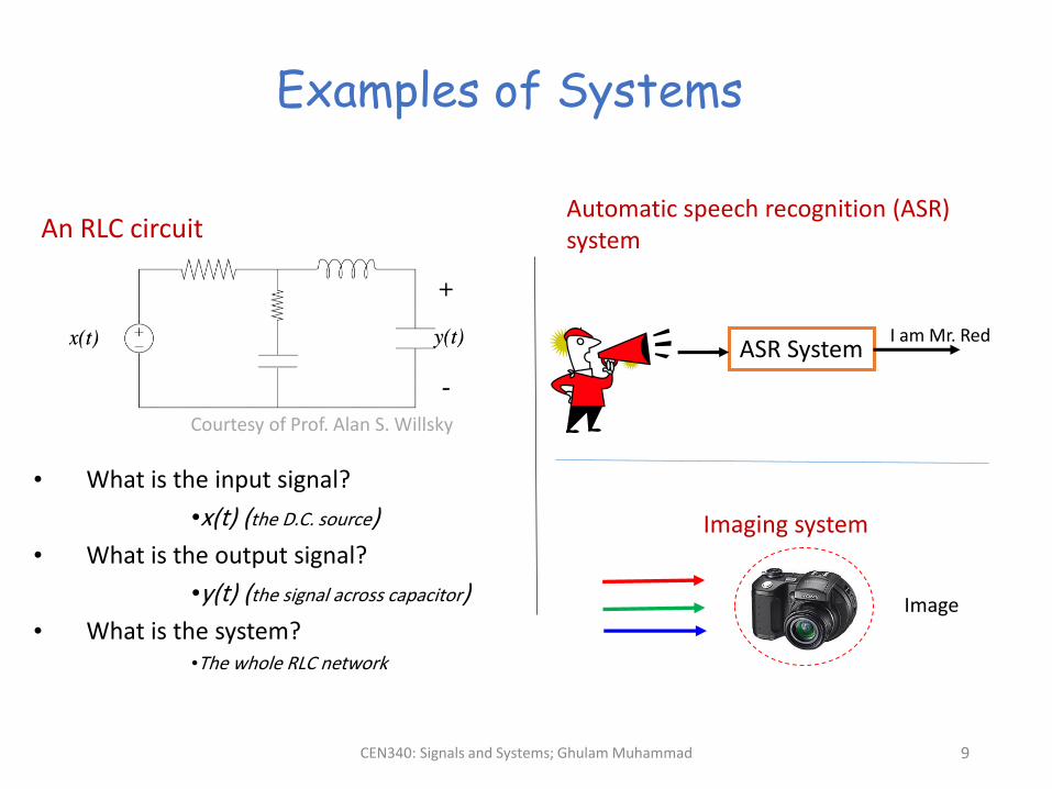
Examples of Systems

An RLC circuit

• What is the input signal?

•x(t) (the D.C. source)

• What is the output signal?

•y(t) (the signal across capacitor)

• What is the system? •The whole RLC network

Courtesy of Prof. Alan S. Willsky

Automatic speech recognition (ASR) system

ASR SystemI am Mr. Red

Image

Imaging system


Drill - 1

1. Most of the signals in this physical world is ……………. (CT signals / DT signals). Choose

the right one.

2. Mention four systems other than those mentioned in the slides.

3. Mention three signals other than those mentioned in the slides.

4. How can we convert a CT signal into a DT signal?

5. Can a system have multiple inputs and multiple outputs?

6. What do you mean by time-domain signal and spatial-domain signal?


• Matlab ® is a software tool for computation in science and engineering.

• Developed, published and trademarked by The MathWorks, Inc.

• Originally developed as a “Matrix Laboratory” but now used in applications in almost all areas of science and engineering.

• It has a rich collection of tool boxes covering basic mathematics, graphics, differential equations, electric/electronic circuits, partial differential equations, simulation problems, control systems, signal processing, image processing, statistics, symbolic computations, etc.

• http://www.mathworks.com/help/pdf_doc/matlab/getstart.pdf

• http://www.mathworks.com/academia/student_center/tutorials/launchpad.html

MATLAB

http://www.mathworks.com/help/pdf_doc/matlab/getstart.pdf

http://www.mathworks.com/academia/student_center/tutorials/launchpad.html


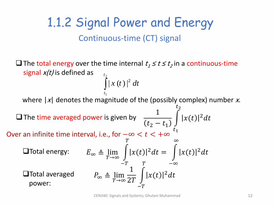
1.1.2 Signal Power and Energy

The total energy over the time internal t1 ≤ t ≤ t2 in a continuous-time signal x(t) is defined as

where |x| denotes the magnitude of the (possibly complex) number x.

2

1

2| ( ) |

t

t

x t dt

1

𝑡2 − 𝑡1න

𝑡1

𝑡2

ሻ𝑥(𝑡 2𝑑𝑡The time averaged power is given by

Continuous-time (CT) signal

Over an infinite time interval, i.e., for −∞ < 𝑡 < +∞

𝐸∞ ≜ lim𝑇→∞

න

−𝑇

𝑇

ሻ𝑥(𝑡 2𝑑𝑡 = න

−∞

∞

ሻ𝑥(𝑡 2𝑑𝑡Total energy:

𝑃∞ ≜ lim𝑇→∞

1

2𝑇න

−𝑇

𝑇

ሻ𝑥(𝑡 2𝑑𝑡Total averaged power:


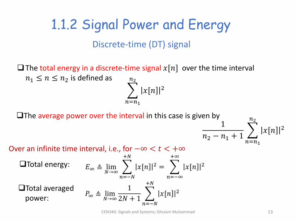
1.1.2 Signal Power and Energy

Discrete-time (DT) signal

The total energy in a discrete-time signal 𝑥[𝑛] over the time interval 𝑛1 ≤ 𝑛 ≤ 𝑛2 is defined as

𝑛=𝑛1

𝑛2

]𝑥[𝑛 2

The average power over the interval in this case is given by1

𝑛2 − 𝑛1 + 1

𝑛=𝑛1

𝑛2

]𝑥[𝑛 2

Over an infinite time interval, i.e., for −∞ < 𝑡 < +∞

Total energy:

Total averaged power:

𝐸∞ ≜ lim𝑁→∞

𝑛=−𝑁

+𝑁

]𝑥[𝑛 2 =

𝑛=−∞

+∞

]𝑥[𝑛 2

𝑃∞ ≜ lim𝑁→∞

1

2𝑁 + 1

𝑛=−𝑁

+𝑁

]𝑥[𝑛 2

CEN340: Signals and Systems; Ghulam Muhammad

14

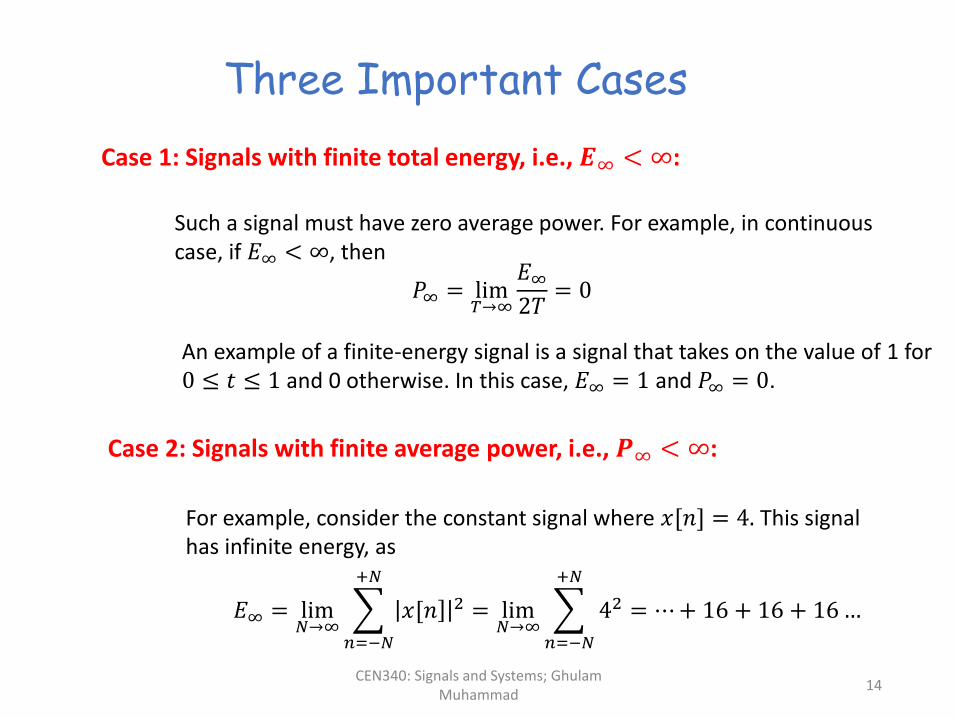
Three Important Cases

Case 1: Signals with finite total energy, i.e., 𝑬∞ < ∞:

Such a signal must have zero average power. For example, in continuous case, if 𝐸∞ < ∞, then

𝑃∞ = lim𝑇→∞

𝐸∞2𝑇

= 0

An example of a finite-energy signal is a signal that takes on the value of 1 for 0 ≤ 𝑡 ≤ 1 and 0 otherwise. In this case, 𝐸∞ = 1 and 𝑃∞ = 0.

Case 2: Signals with finite average power, i.e., 𝑷∞ < ∞:

For example, consider the constant signal where 𝑥[𝑛] = 4. This signal has infinite energy, as

𝐸∞ = lim𝑁→∞

𝑛=−𝑁

+𝑁

]𝑥[𝑛 2 = lim𝑁→∞

𝑛=−𝑁

+𝑁

42 = ⋯+ 16 + 16 + 16…


15

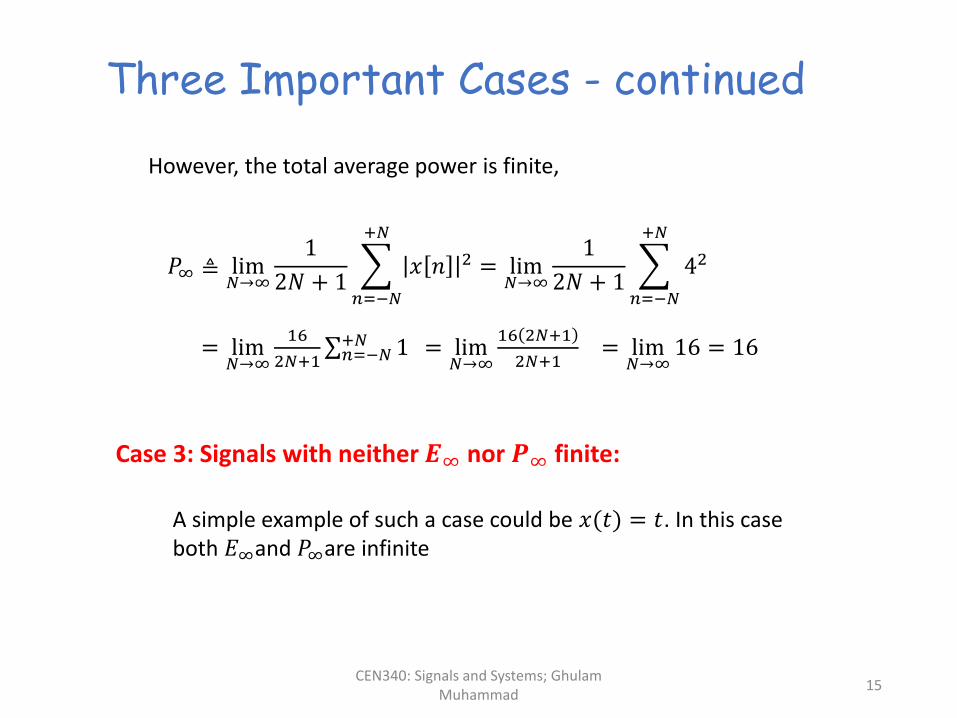
However, the total average power is finite,

Three Important Cases - continued

𝑃∞ ≜ lim𝑁→∞

1

2𝑁 + 1

𝑛=−𝑁

+𝑁

𝑥 𝑛 2 = lim𝑁→∞

1

2𝑁 + 1

𝑛=−𝑁

+𝑁

42

= lim𝑁→∞

16

2𝑁+1σ𝑛=−𝑁+𝑁 1 = lim

𝑁→∞

16 2𝑁+1

2𝑁+1= lim

𝑁→∞16 = 16

Case 3: Signals with neither 𝑬∞ nor 𝑷∞ finite:

A simple example of such a case could be 𝑥(𝑡ሻ = 𝑡. In this case both 𝐸∞and 𝑃∞are infinite


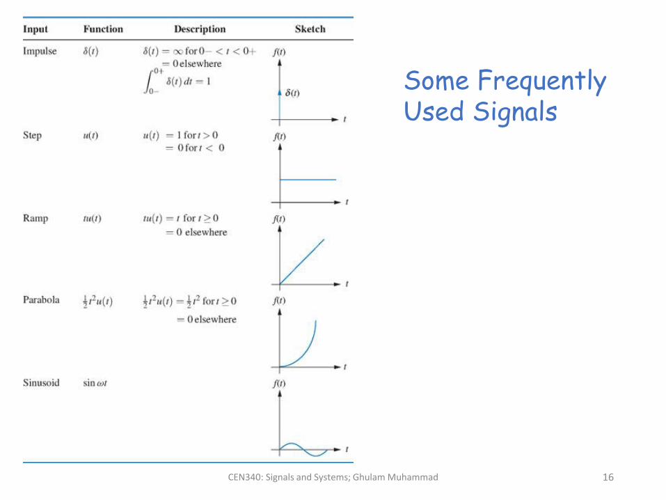
Some Frequently Used Signals


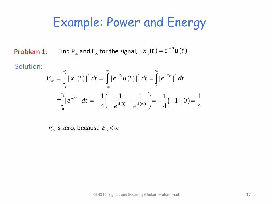
Example: Power and Energy

Problem 1: Find P and E for the signal,2

1( ) ( )tx t e u t

Solution:

2 2 2 2 2

1

0

4

4(0) 4( )

0

| ( ) | | ( ) | | |

1 1 1 1 1 = | | 1 0

4 4 4

t t

t

E x t dt e u t dt e dt

e dte e

P is zero, because E <


18

1.2 Transformations of the Independent Variable

The transformation of a signal is one of the central concepts in

the field of signals and systems.

We will focus on a very limited but important class of signal transformations that involves the modifications of the independent variable, i.e., the time axis.

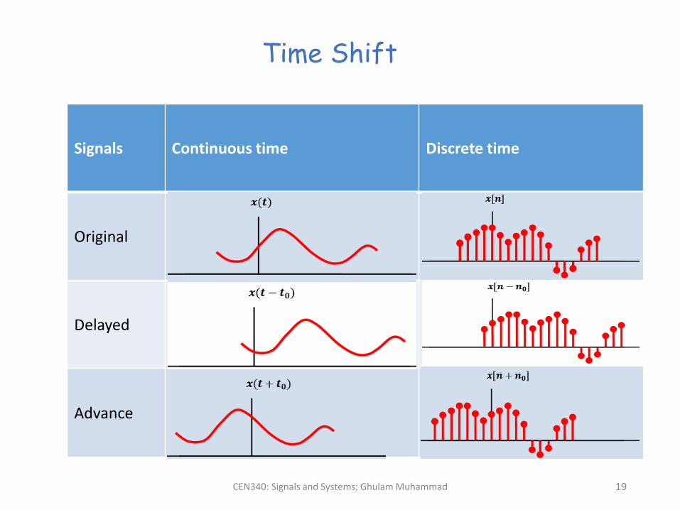
(A) Time Shift

The original and the shifted signals are identical in shape, but are displaced or shifted along the time-axis with respect to each other. Signals could be termed as delayed or advanced in this case.


Time Shift

Signals Continuous time Discrete time

Original

Delayed

Advance


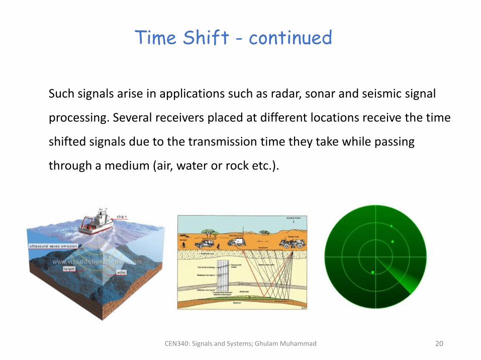
Time Shift - continued

Such signals arise in applications such as radar, sonar and seismic signal

processing. Several receivers placed at different locations receive the time

shifted signals due to the transmission time they take while passing

through a medium (air, water or rock etc.).


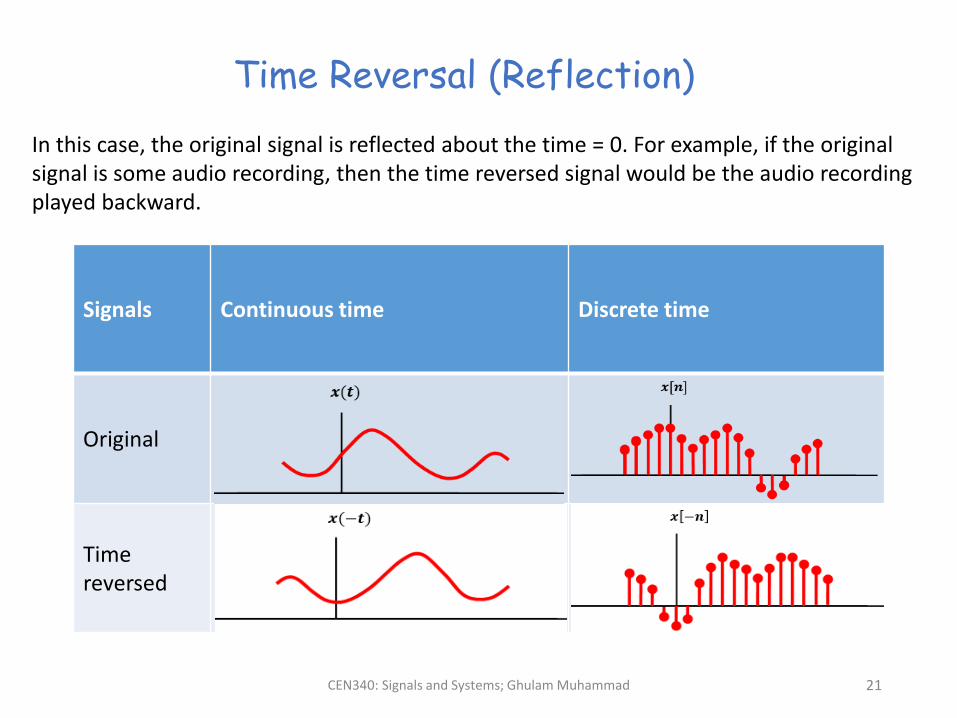
Time Reversal (Reflection)

In this case, the original signal is reflected about the time = 0. For example, if the original signal is some audio recording, then the time reversed signal would be the audio recording played backward.

Signals Continuous time Discrete time

Original

Time reversed


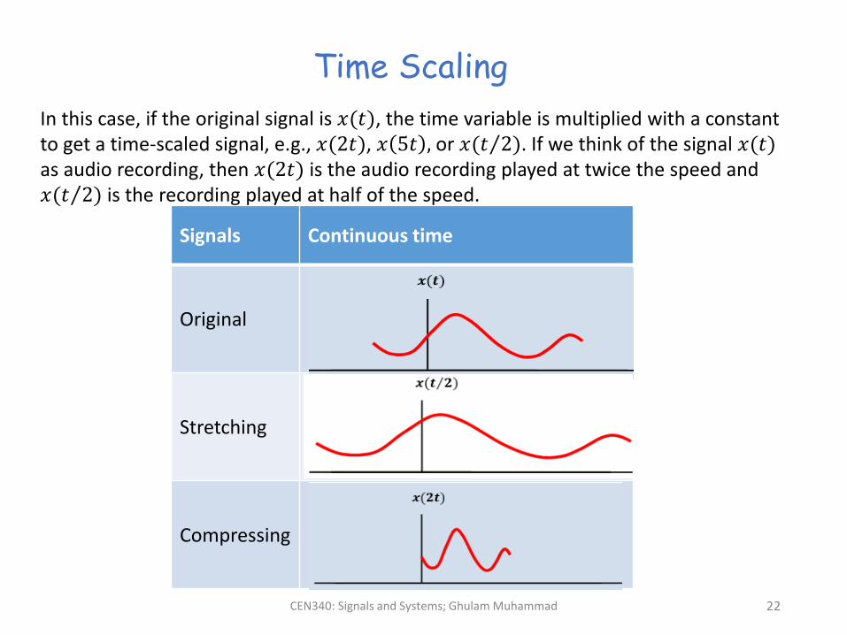
Time Scaling

In this case, if the original signal is 𝑥(𝑡ሻ, the time variable is multiplied with a constant to get a time-scaled signal, e.g., 𝑥(2𝑡ሻ, 𝑥 5𝑡 , or 𝑥( Τ𝑡 2ሻ. If we think of the signal 𝑥(𝑡ሻas audio recording, then 𝑥(2𝑡ሻ is the audio recording played at twice the speed and 𝑥( Τ𝑡 2ሻ is the recording played at half of the speed.

Signals Continuous time

Original

Stretching

Compressing


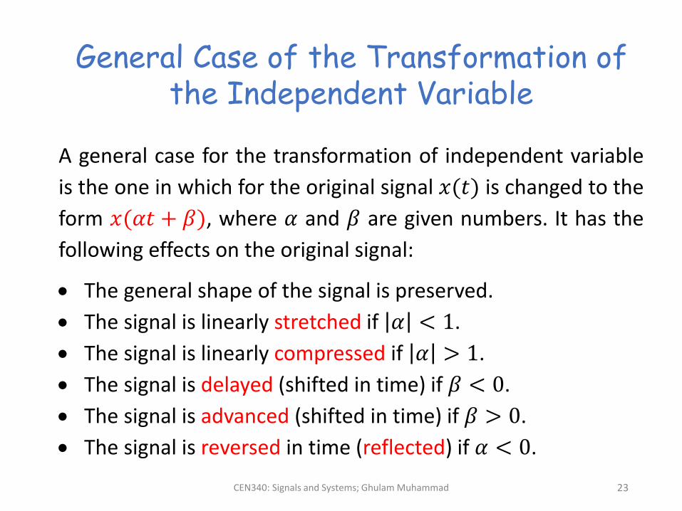
General Case of the Transformation of the Independent Variable

A general case for the transformation of independent variable

is the one in which for the original signal 𝑥(𝑡ሻ is changed to the

form 𝑥(𝛼𝑡 + 𝛽ሻ, where 𝛼 and 𝛽 are given numbers. It has the

following effects on the original signal:

The general shape of the signal is preserved.

The signal is linearly stretched if 𝛼 < 1.

The signal is linearly compressed if 𝛼 > 1.

The signal is delayed (shifted in time) if 𝛽 < 0.

The signal is advanced (shifted in time) if 𝛽 > 0.

The signal is reversed in time (reflected) if 𝛼 < 0.


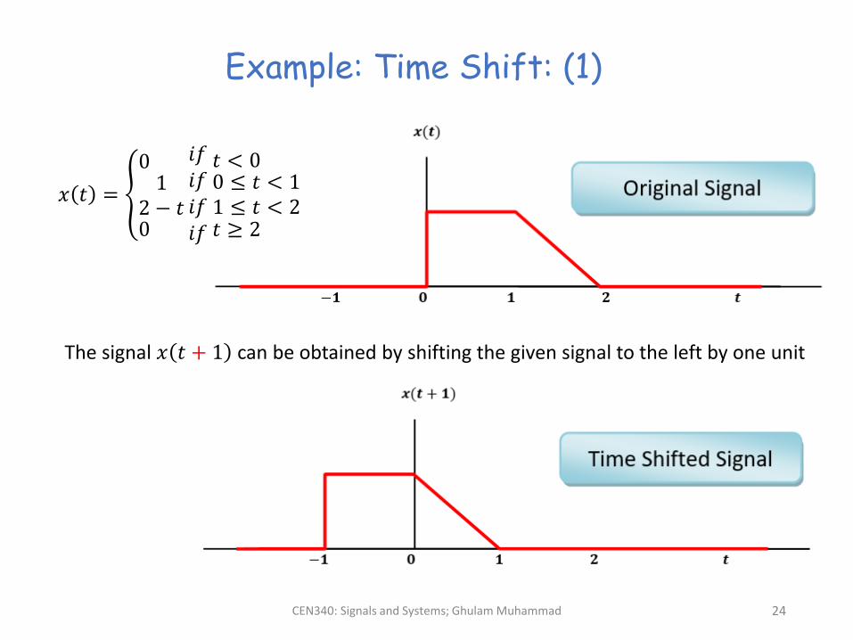
Example: Time Shift: (1)

𝑥 𝑡 = ൞

01

2 − 𝑡0

𝑖𝑓𝑖𝑓𝑖𝑓𝑖𝑓

𝑡 < 00 ≤ 𝑡 < 11 ≤ 𝑡 < 2𝑡 ≥ 2

The signal 𝑥 𝑡 + 1 can be obtained by shifting the given signal to the left by one unit


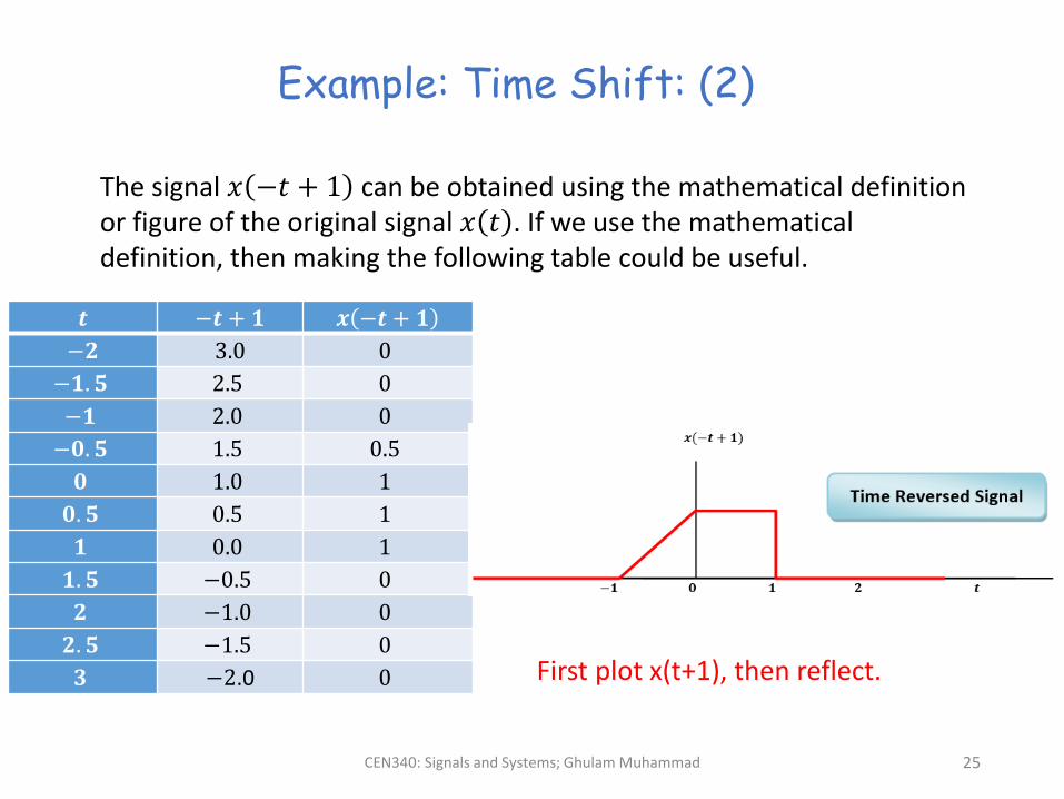
Example: Time Shift: (2)

The signal 𝑥 −𝑡 + 1 can be obtained using the mathematical definition or figure of the original signal 𝑥 𝑡 . If we use the mathematical definition, then making the following table could be useful.

𝒕 −𝒕 + 𝟏 𝒙 −𝒕 + 𝟏

−𝟐 3.0 0

−𝟏. 𝟓 2.5 0

−𝟏 2.0 0

−𝟎. 𝟓 1.5 0.5

𝟎 1.0 1

𝟎. 𝟓 0.5 1

𝟏 0.0 1

𝟏. 𝟓 −0.5 0

𝟐 −1.0 0

𝟐. 𝟓 −1.5 0

𝟑 −2.0 0 First plot x(t+1), then reflect.


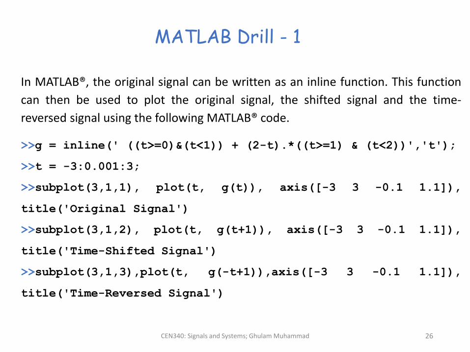
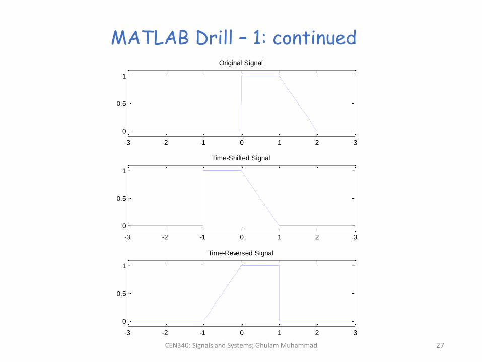
MATLAB Drill - 1

In MATLAB®, the original signal can be written as an inline function. This function

can then be used to plot the original signal, the shifted signal and the time-

reversed signal using the following MATLAB® code.

>>g = inline(' ((t>=0)&(t<1)) + (2-t).*((t>=1) & (t<2))','t');

>>t = -3:0.001:3;

>>subplot(3,1,1), plot(t, g(t)), axis([-3 3 -0.1 1.1]),

title('Original Signal')

>>subplot(3,1,2), plot(t, g(t+1)), axis([-3 3 -0.1 1.1]),

title('Time-Shifted Signal')

>>subplot(3,1,3),plot(t, g(-t+1)),axis([-3 3 -0.1 1.1]),

title('Time-Reversed Signal')


MATLAB Drill – 1: continued

-3 -2 -1 0 1 2 3

0

0.5

1

Original Signal

-3 -2 -1 0 1 2 3

0

0.5

1

Time-Shifted Signal

-3 -2 -1 0 1 2 3

0

0.5

1

Time-Reversed Signal


28

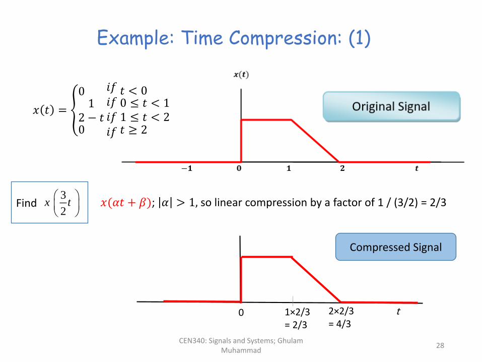
Example: Time Compression: (1)

𝑥 𝑡 = ൞

01

2 − 𝑡0

𝑖𝑓𝑖𝑓𝑖𝑓𝑖𝑓

𝑡 < 00 ≤ 𝑡 < 11 ≤ 𝑡 < 2𝑡 ≥ 2

Find 3

2x t

𝑥(𝛼𝑡 + 𝛽ሻ; 𝛼 > 1, so linear compression by a factor of 1 / (3/2) = 2/3

0 1×2/3 = 2/3

2×2/3 = 4/3

t

Compressed Signal


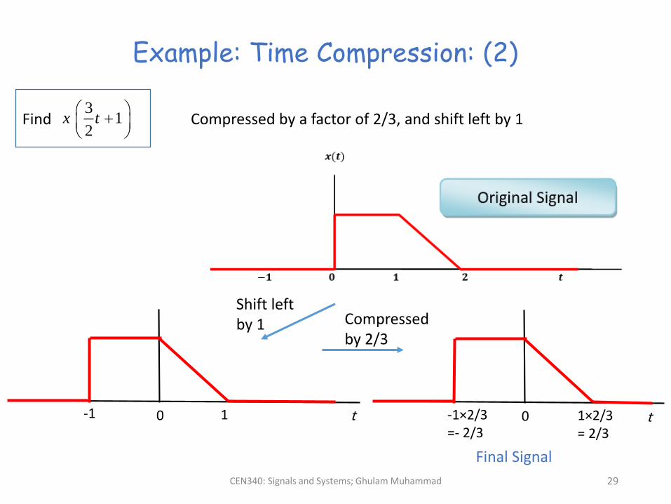
Example: Time Compression: (2)

Find 3

12

x t

Compressed by a factor of 2/3, and shift left by 1

0 1 t 0-1×2/3 =- 2/3

1×2/3 = 2/3

t-1

Shift left by 1 Compressed

by 2/3

Final Signal


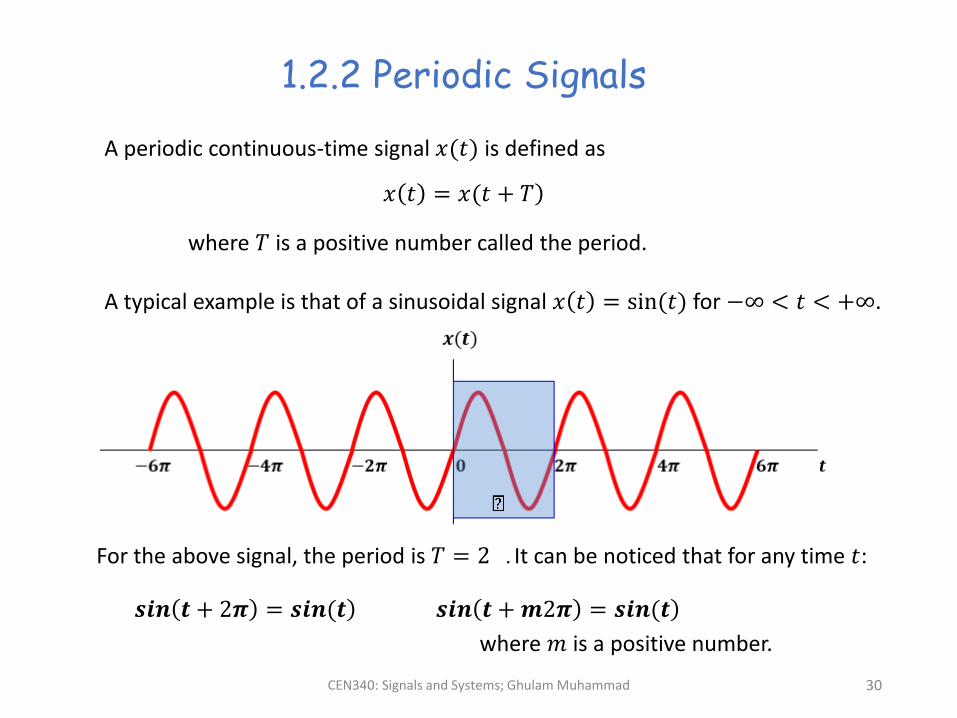
1.2.2 Periodic Signals

A periodic continuous-time signal 𝑥(𝑡ሻ is defined as

ሻ𝑥 𝑡 = 𝑥(𝑡 + 𝑇

where 𝑇 is a positive number called the period.

A typical example is that of a sinusoidal signal 𝑥 𝑡 = sin(𝑡ሻ for −∞ < 𝑡 < +∞.

For the above signal, the period is 𝑇 = 2 . It can be noticed that for any time 𝑡:

ሻ𝒔𝒊𝒏 𝒕 + 2𝝅 = 𝒔𝒊𝒏(𝒕 ሻ𝒔𝒊𝒏 𝒕 +𝒎2𝝅 = 𝒔𝒊𝒏(𝒕

where 𝑚 is a positive number.


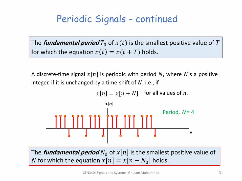
Periodic Signals - continued

The fundamental period 𝑇0 of 𝑥(𝑡ሻ is the smallest positive value of 𝑇

for which the equation 𝑥 𝑡 = 𝑥(𝑡 + 𝑇ሻ holds.

A discrete-time signal 𝑥[𝑛] is periodic with period 𝑁, where 𝑁is a positive

integer, if it is unchanged by a time-shift of 𝑁, i.e., if

]𝑥 𝑛 = 𝑥[𝑛 + 𝑁 for all values of 𝑛.

The fundamental period 𝑁0 of 𝑥[𝑛] is the smallest positive value of 𝑁 for which the equation 𝑥[𝑛] = 𝑥[𝑛 + 𝑁0] holds.

Period, N = 4


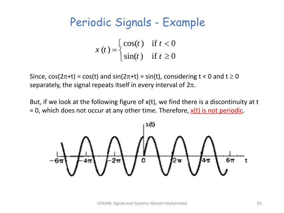
Periodic Signals - Example

cos( ) if 0( )

sin( ) if 0

t tx t

t t

Since, cos(2+t) = cos(t) and sin(2+t) = sin(t), considering t < 0 and t 0 separately, the signal repeats itself in every interval of 2.

But, if we look at the following figure of x(t), we find there is a discontinuity at t = 0, which does not occur at any other time. Therefore, x(t) is not periodic.


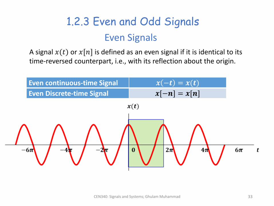
1.2.3 Even and Odd Signals

A signal 𝑥(𝑡ሻ or 𝑥[𝑛] is defined as an even signal if it is identical to its time-reversed counterpart, i.e., with its reflection about the origin.

Even Signals

Even continuous-time Signal 𝒙 −𝒕 = 𝒙(𝒕ሻ

Even Discrete-time Signal 𝒙[−𝒏] = 𝒙[𝒏]


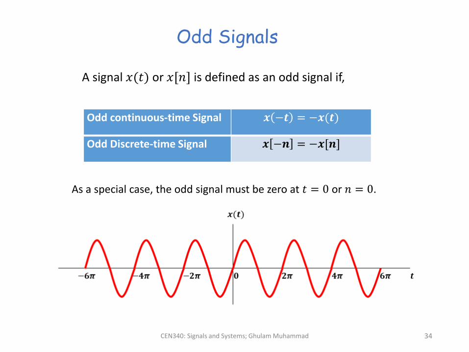
Odd Signals

A signal 𝑥(𝑡ሻ or 𝑥[𝑛] is defined as an odd signal if,

Odd continuous-time Signal 𝒙 −𝒕 = −𝒙(𝒕ሻ

Odd Discrete-time Signal 𝒙 −𝒏 = −𝒙[𝒏]

As a special case, the odd signal must be zero at 𝑡 = 0 or 𝑛 = 0.


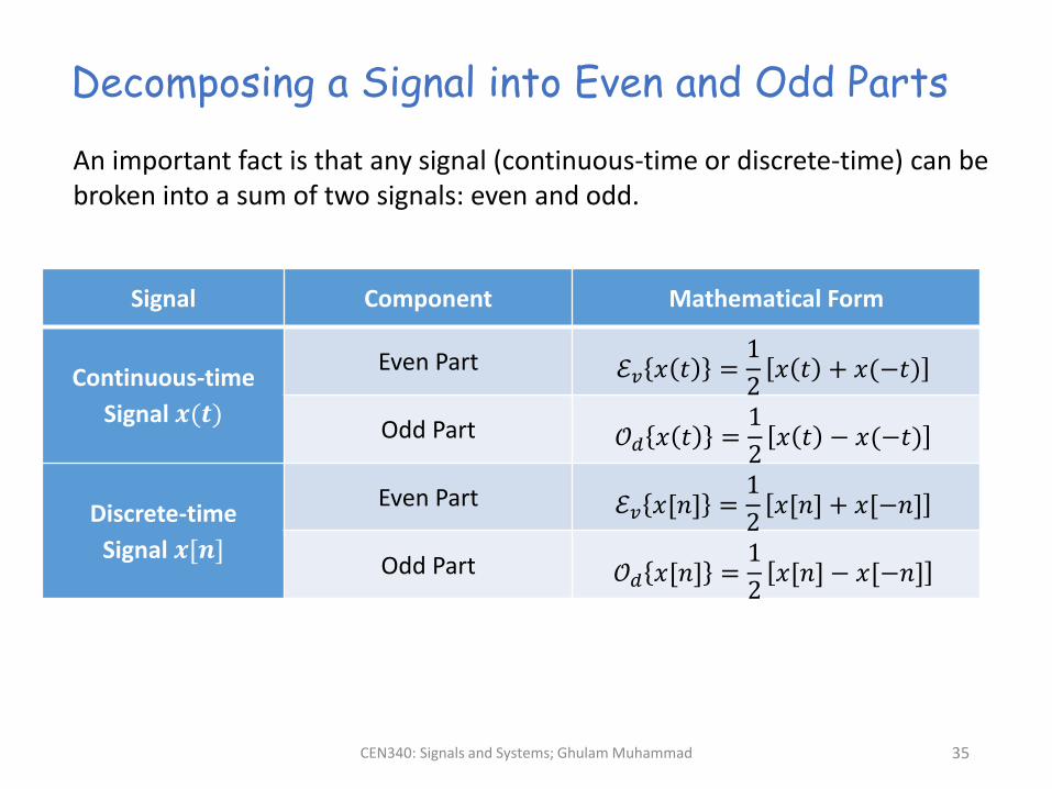
Decomposing a Signal into Even and Odd Parts

An important fact is that any signal (continuous-time or discrete-time) can be broken into a sum of two signals: even and odd.

Signal Component Mathematical Form

Continuous-time

Signal 𝒙(𝒕ሻ

Even Part ℰ𝑣 𝑥 𝑡 =1

2𝑥 𝑡 + 𝑥(−𝑡ሻ

Odd Part 𝒪𝑑 𝑥 𝑡 =1

2𝑥 𝑡 − 𝑥(−𝑡ሻ

Discrete-time

Signal 𝒙[𝒏]

Even Part ℰ𝑣 𝑥[𝑛] =1

2𝑥[𝑛] + 𝑥[−𝑛]

Odd Part 𝒪𝑑 𝑥[𝑛] =1

2𝑥[𝑛] − 𝑥[−𝑛]


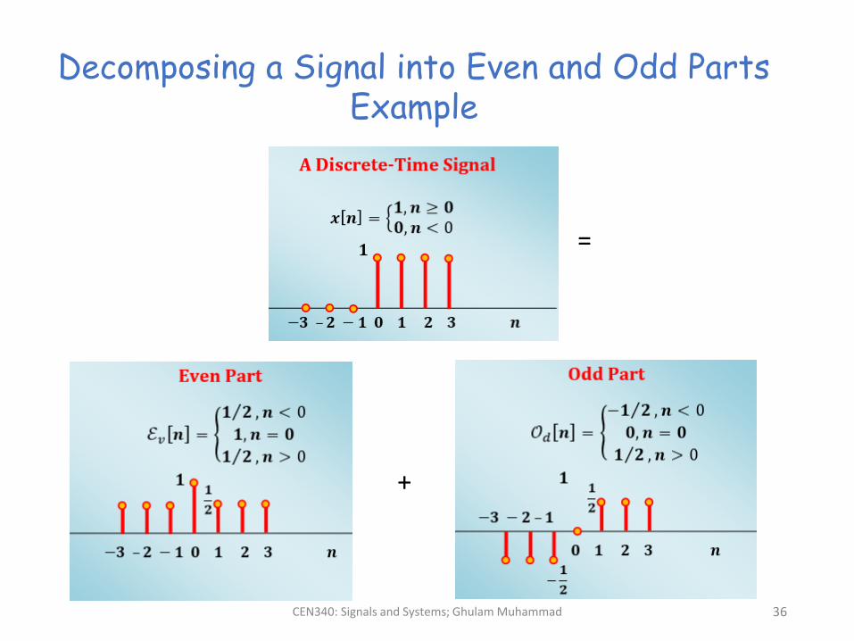
Decomposing a Signal into Even and Odd PartsExample

+

=


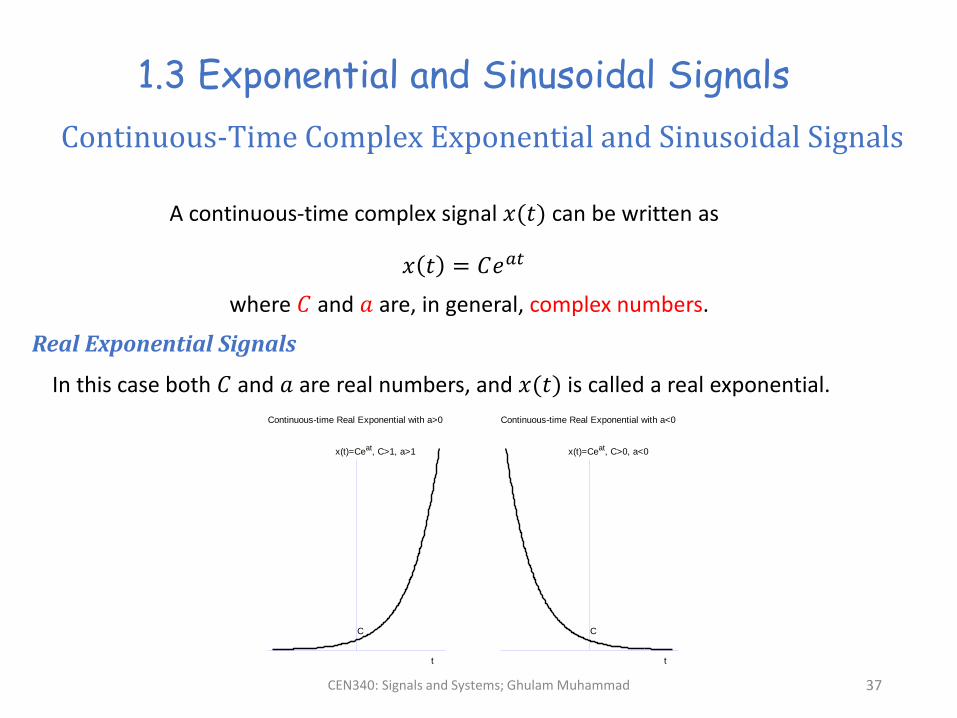
1.3 Exponential and Sinusoidal Signals

Continuous-Time Complex Exponential and Sinusoidal Signals

A continuous-time complex signal 𝑥(𝑡ሻ can be written as

𝑥 𝑡 = 𝐶𝑒𝑎𝑡

where 𝐶 and 𝑎 are, in general, complex numbers.

In this case both 𝐶 and 𝑎 are real numbers, and 𝑥(𝑡ሻ is called a real exponential.

Real Exponential Signals

Continuous-time Real Exponential with a>0

C

x(t)=Ceat, C>1, a>1

t

Continuous-time Real Exponential with a<0

C

x(t)=Ceat, C>0, a<0

t


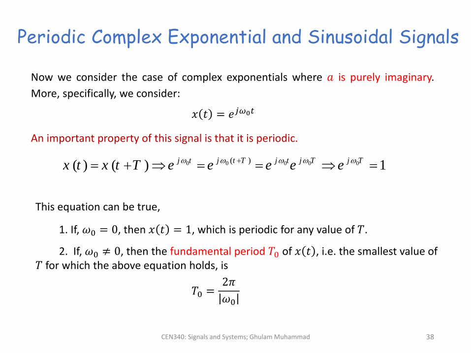
Periodic Complex Exponential and Sinusoidal Signals

Now we consider the case of complex exponentials where 𝑎 is purely imaginary.

More, specifically, we consider:

𝑥 𝑡 = 𝑒𝑗𝜔0𝑡

An important property of this signal is that it is periodic.

0 0 0 0 0( )( ) ( ) 1

j t j t T j t j T j Tx t x t T e e e e e

This equation can be true,

1. If, 𝜔0 = 0, then 𝑥 𝑡 = 1, which is periodic for any value of 𝑇.

2. If, 𝜔0 ≠ 0, then the fundamental period 𝑇0 of 𝑥 𝑡 , i.e. the smallest value of 𝑇 for which the above equation holds, is

𝑇0 =2𝜋

𝜔0


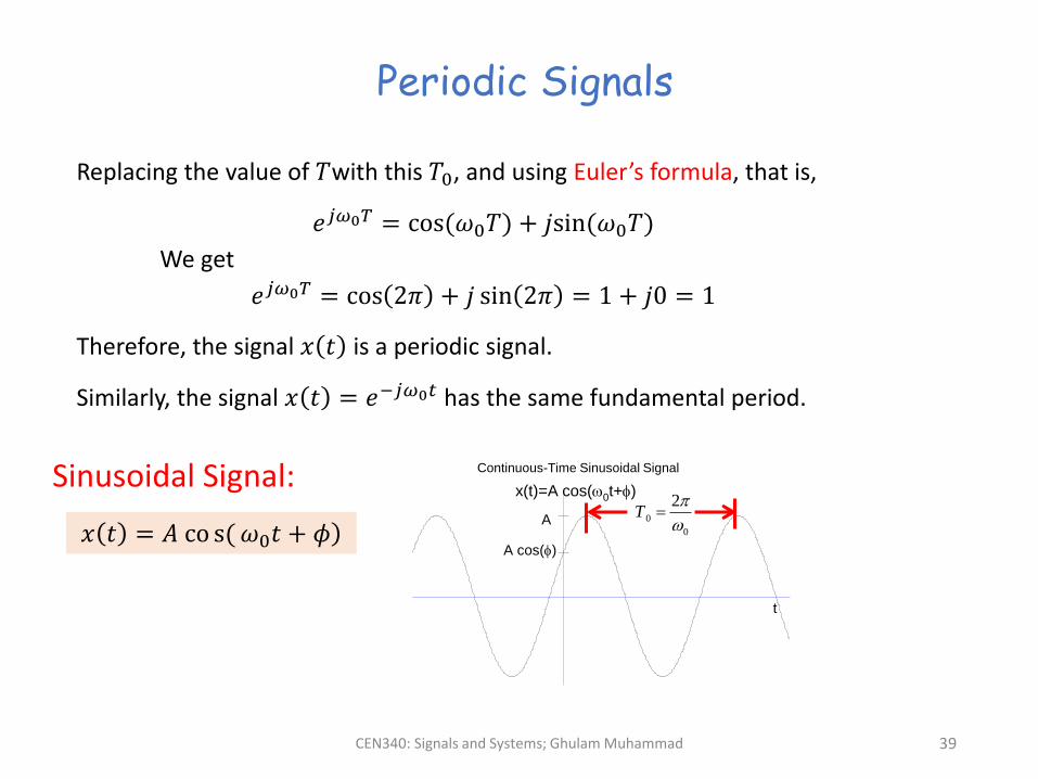
Periodic Signals

Replacing the value of 𝑇with this 𝑇0, and using Euler’s formula, that is,

𝑒𝑗𝜔0𝑇 = cos(𝜔0𝑇ሻ + 𝑗sin(𝜔0𝑇ሻ

We get

𝑒𝑗𝜔0𝑇 = cos 2𝜋 + 𝑗 sin 2𝜋 = 1 + 𝑗0 = 1

Therefore, the signal 𝑥 𝑡 is a periodic signal.

Similarly, the signal 𝑥 𝑡 = 𝑒−𝑗𝜔0𝑡 has the same fundamental period.

Sinusoidal Signal:

ሻ𝑥 𝑡 = 𝐴 co s(𝜔0𝑡 + 𝜙

Continuous-Time Sinusoidal Signal

x(t)=A cos(0t+)

t

A

A cos()

0

0

2T


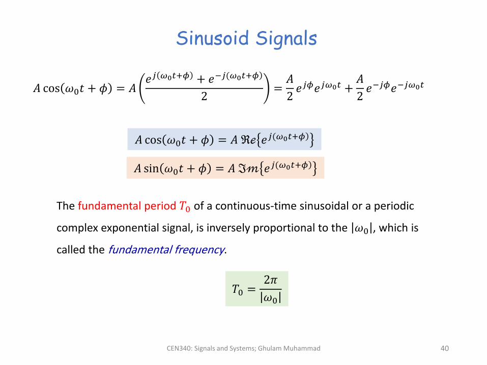
𝐴 cos 𝜔0𝑡 + 𝜙 = 𝐴𝑒𝑗 𝜔0𝑡+𝜙 + 𝑒 ሻ−𝑗(𝜔0𝑡+𝜙

2=𝐴

2𝑒𝑗𝜙𝑒𝑗𝜔0𝑡 +

𝐴

2𝑒−𝑗𝜙𝑒−𝑗𝜔0𝑡

Sinusoid Signals

𝐴 cos 𝜔0𝑡 + 𝜙 = 𝐴 ℜℯ 𝑒 ሻ𝑗(𝜔0𝑡+𝜙

𝐴 sin 𝜔0𝑡 + 𝜙 = 𝐴 ℑ𝓂 𝑒 ሻ𝑗(𝜔0𝑡+𝜙

The fundamental period 𝑇0 of a continuous-time sinusoidal or a periodic

complex exponential signal, is inversely proportional to the 𝜔0 , which is

called the fundamental frequency.

𝑇0 =2𝜋

𝜔0


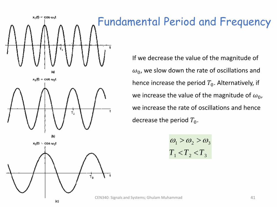
If we decrease the value of the magnitude of

𝜔0, we slow down the rate of oscillations and

hence increase the period 𝑇0. Alternatively, if

we increase the value of the magnitude of 𝜔0,

we increase the rate of oscillations and hence

decrease the period 𝑇0.

Fundamental Period and Frequency

1 2 3

1 2 3T T T


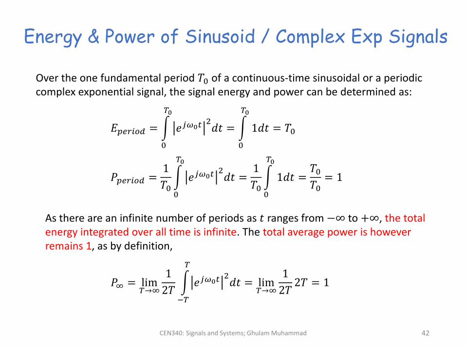
Energy & Power of Sinusoid / Complex Exp Signals

Over the one fundamental period 𝑇0 of a continuous-time sinusoidal or a periodic complex exponential signal, the signal energy and power can be determined as:

𝐸𝑝𝑒𝑟𝑖𝑜𝑑 = න

0

𝑇0

𝑒𝑗𝜔0𝑡2𝑑𝑡 = න

0

𝑇0

1𝑑𝑡 = 𝑇0

𝑃𝑝𝑒𝑟𝑖𝑜𝑑 =1

𝑇0න

0

𝑇0

𝑒𝑗𝜔0𝑡2𝑑𝑡 =

1

𝑇0න

0

𝑇0

1𝑑𝑡 =𝑇0𝑇0

= 1

As there are an infinite number of periods as 𝑡 ranges from −∞ to +∞, the total energy integrated over all time is infinite. The total average power is however remains 1, as by definition,

𝑃∞ = lim𝑇→∞

1

2𝑇න

−𝑇

𝑇

𝑒𝑗𝜔0𝑡2𝑑𝑡 = lim

𝑇→∞

1

2𝑇2𝑇 = 1


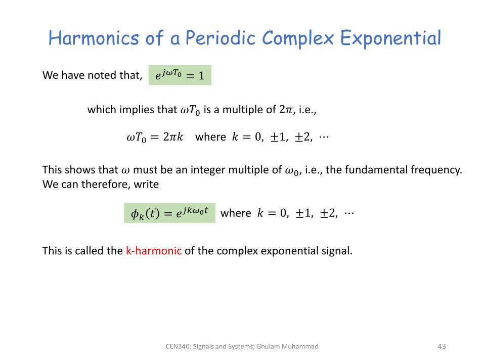
Harmonics of a Periodic Complex Exponential

We have noted that, 𝑒𝑗𝜔𝑇0 = 1

which implies that 𝜔𝑇0 is a multiple of 2𝜋, i.e.,

𝜔𝑇0 = 2𝜋𝑘 where 𝑘 = 0, ±1, ±2, ⋯

This shows that 𝜔 must be an integer multiple of 𝜔0, i.e., the fundamental frequency. We can therefore, write

𝜙𝑘 𝑡 = 𝑒𝑗𝑘𝜔0𝑡 where 𝑘 = 0, ±1, ±2, ⋯

This is called the k-harmonic of the complex exponential signal.


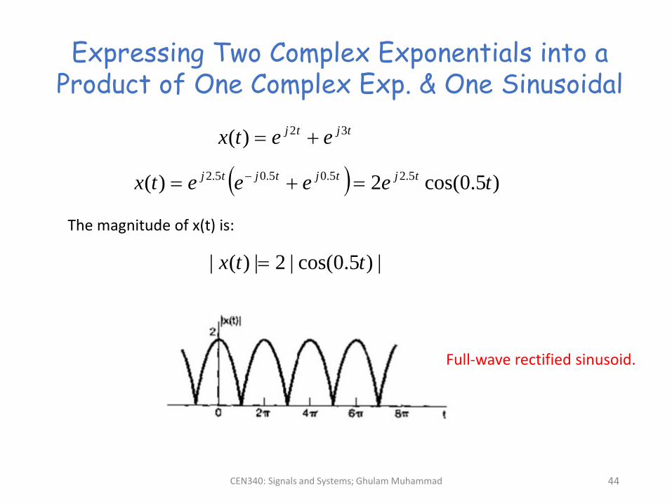
Expressing Two Complex Exponentials into a Product of One Complex Exp. & One Sinusoidal

tjtj eetx 32)(

)5.0cos(2)( 5.25.05.05.2 teeeetx tjtjtjtj

|)5.0cos(|2|)(| ttx

The magnitude of x(t) is:

Full-wave rectified sinusoid.


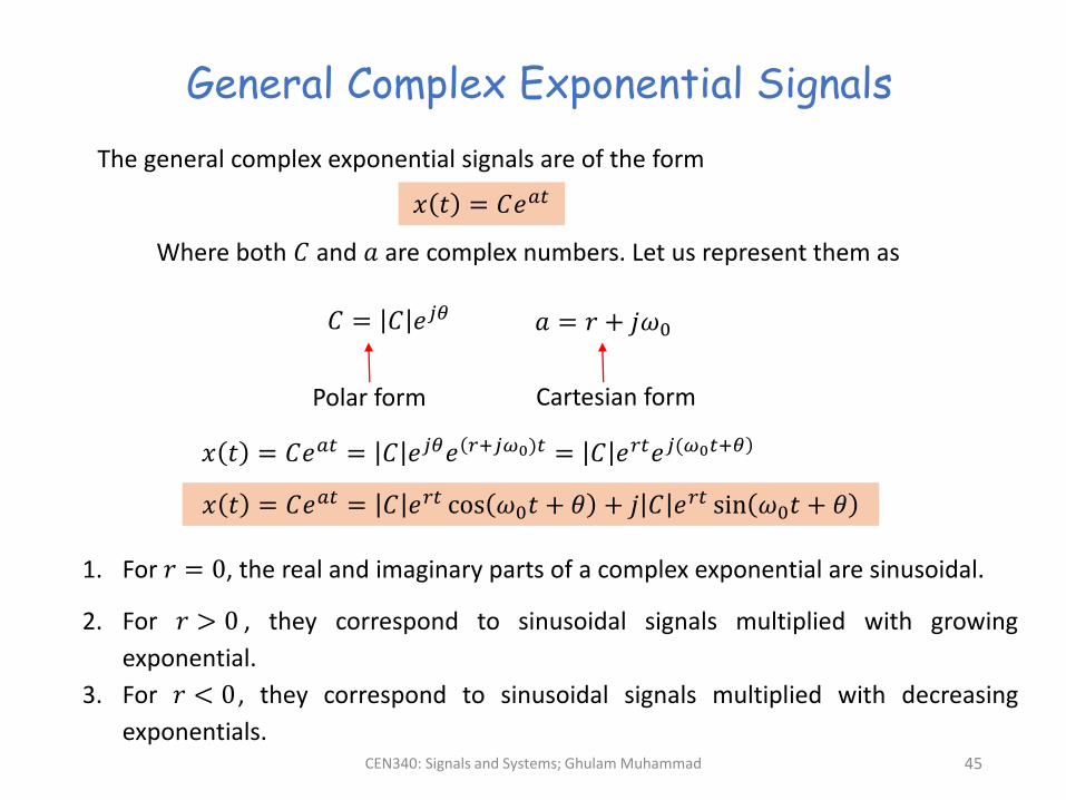
General Complex Exponential Signals

The general complex exponential signals are of the form

𝑥 𝑡 = 𝐶𝑒𝑎𝑡

Where both 𝐶 and 𝑎 are complex numbers. Let us represent them as

𝐶 = 𝐶 𝑒𝑗𝜃 𝑎 = 𝑟 + 𝑗𝜔0

Polar form Cartesian form

𝑥 𝑡 = 𝐶𝑒𝑎𝑡 = 𝐶 𝑒𝑗𝜃𝑒(𝑟+𝑗𝜔0ሻ𝑡 = 𝐶 𝑒𝑟𝑡𝑒 ሻ𝑗(𝜔0𝑡+𝜃

𝑥 𝑡 = 𝐶𝑒𝑎𝑡 = 𝐶 𝑒𝑟𝑡 cos 𝜔0𝑡 + 𝜃 + 𝑗 𝐶 𝑒𝑟𝑡 sin 𝜔0𝑡 + 𝜃

1. For 𝑟 = 0, the real and imaginary parts of a complex exponential are sinusoidal.

2. For 𝑟 > 0 , they correspond to sinusoidal signals multiplied with growing

exponential.

3. For 𝑟 < 0 , they correspond to sinusoidal signals multiplied with decreasing

exponentials.


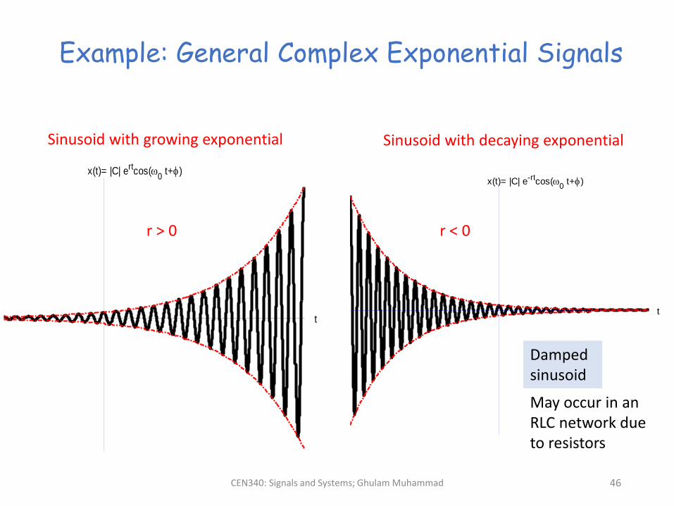
x(t)= |C| ertcos(0 t+)

t

x(t)= |C| e-rtcos(0 t+)

t

Example: General Complex Exponential Signals

Sinusoid with growing exponential Sinusoid with decaying exponential

r > 0 r < 0

Damped sinusoid

May occur in an RLC network due to resistors


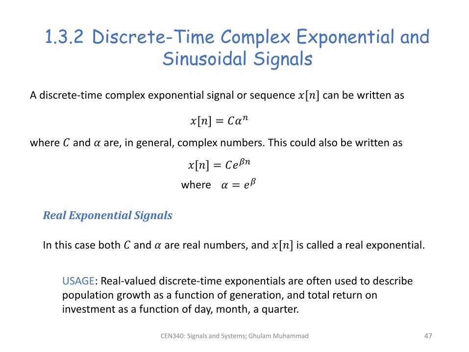
1.3.2 Discrete-Time Complex Exponential and Sinusoidal Signals

A discrete-time complex exponential signal or sequence 𝑥[𝑛] can be written as

𝑥[𝑛] = 𝐶𝛼𝑛

where 𝐶 and 𝛼 are, in general, complex numbers. This could also be written as

𝑥[𝑛] = 𝐶𝑒𝛽𝑛

where 𝛼 = 𝑒𝛽

Real Exponential Signals

In this case both 𝐶 and 𝛼 are real numbers, and 𝑥[𝑛] is called a real exponential.

USAGE: Real-valued discrete-time exponentials are often used to describe population growth as a function of generation, and total return on investment as a function of day, month, a quarter.


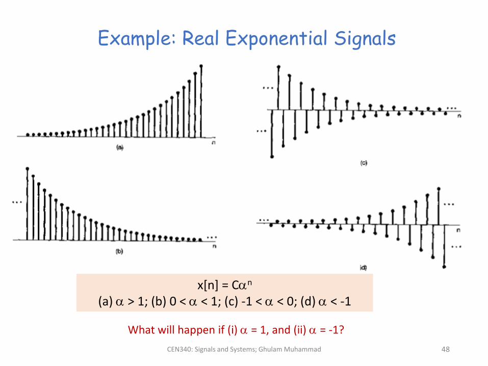
x[n] = Cn

(a) > 1; (b) 0 < < 1; (c) -1 < < 0; (d) < -1

Example: Real Exponential Signals

What will happen if (i) = 1, and (ii) = -1?


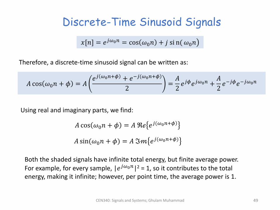
Discrete-Time Sinusoid Signals

൯𝑥[𝑛] = 𝑒𝑗𝜔0𝑛 = cos 𝜔0𝑛 + 𝑗 si n(𝜔0𝑛

𝐴 cos 𝜔0𝑛 + 𝜙 = 𝐴𝑒𝑗 𝜔0𝑛+𝜙 + 𝑒 ሻ−𝑗(𝜔0𝑛+𝜙

2=𝐴

2𝑒𝑗𝜙𝑒𝑗𝜔0𝑛 +

𝐴

2𝑒−𝑗𝜙𝑒−𝑗𝜔0𝑛

Therefore, a discrete-time sinusoid signal can be written as:

𝐴 sin(𝜔0𝑛 + 𝜙ሻ = 𝐴 ℑ𝓂 𝑒𝑗(𝜔0𝑛+𝜙ሻ

𝐴 cos 𝜔0𝑛 + 𝜙 = 𝐴 ℜℯ 𝑒 ሻ𝑗(𝜔0𝑛+𝜙

Using real and imaginary parts, we find:

Both the shaded signals have infinite total energy, but finite average power.

For example, for every sample, |𝑒𝑗𝜔0𝑛|2 = 1, so it contributes to the total energy, making it infinite; however, per point time, the average power is 1.


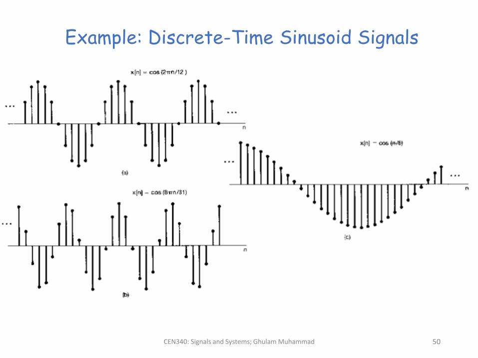
Example: Discrete-Time Sinusoid Signals


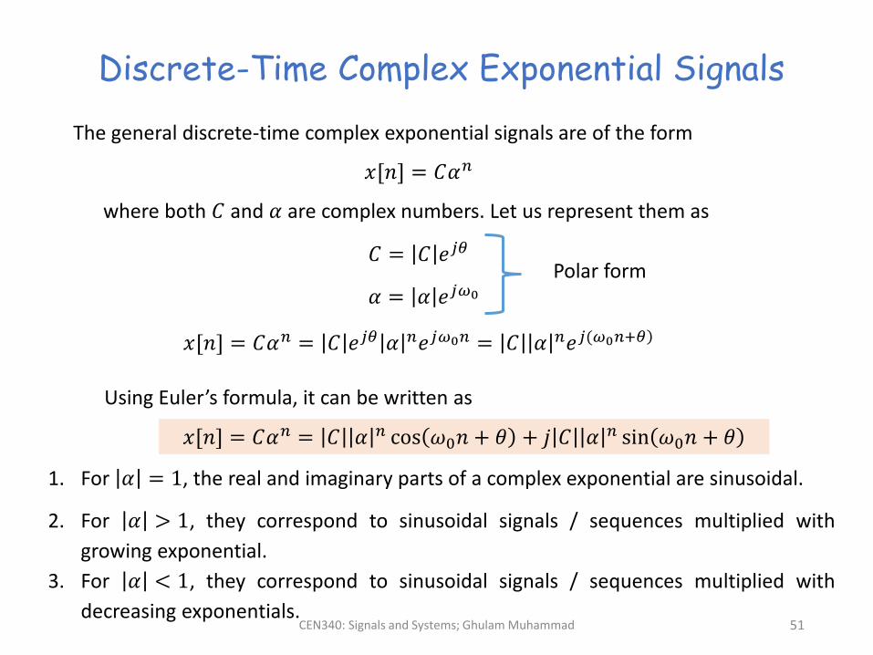
Discrete-Time Complex Exponential Signals

The general discrete-time complex exponential signals are of the form

𝑥[𝑛] = 𝐶𝛼𝑛

where both 𝐶 and 𝛼 are complex numbers. Let us represent them as

𝐶 = 𝐶 𝑒𝑗𝜃

𝛼 = 𝛼 𝑒𝑗𝜔0

𝑥[𝑛] = 𝐶𝛼𝑛 = 𝐶 𝑒𝑗𝜃 𝛼 𝑛𝑒𝑗𝜔0𝑛 = 𝐶 𝛼 𝑛𝑒 ሻ𝑗(𝜔0𝑛+𝜃

Polar form

Using Euler’s formula, it can be written as

𝑥[𝑛] = 𝐶𝛼𝑛 = 𝐶 𝛼 𝑛 cos 𝜔0𝑛 + 𝜃 + 𝑗 𝐶 𝛼 𝑛 sin 𝜔0𝑛 + 𝜃

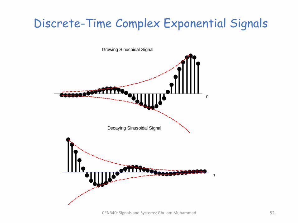
1. For 𝛼 = 1, the real and imaginary parts of a complex exponential are sinusoidal.

2. For 𝛼 > 1, they correspond to sinusoidal signals / sequences multiplied with

growing exponential.

3. For 𝛼 < 1, they correspond to sinusoidal signals / sequences multiplied with

decreasing exponentials.



Growing Sinusoidal Signal

n

Decaying Sinusoidal Signal

n

Growing Sinusoidal Signal

n

Decaying Sinusoidal Signal

n



There are many similarities between continuous-time and discrete-time signals. But also there are many important differences. One of them is related with the

discrete-time exponential signal 𝑒𝑗𝜔0𝑛

The following properties were found with regard to the continuous-time

exponential signal 𝑒𝑗𝜔0𝑡:

1. The larger the magnitude of 𝜔0, the higher is the rate of oscillations in the

signal;

2. 𝑒𝑗𝜔0𝑡 is periodic for any value of 𝜔0.

To see the difference for the first property, consider the discrete-time complex exponential:

𝑒𝑗(𝜔0+2𝜋ሻ𝑛 = 𝑒𝑗2𝜋𝑛𝑒𝑗𝜔0𝑛 = 𝑒𝑗𝜔0𝑛

This shows that the exponential at 𝜔0 + 2𝜋 is the same as that at frequency 𝜔0



In case of continuous-time exponential, the signals 𝑒𝑗𝜔0𝑡 are all distinct for distinct values of 𝜔0.

In discrete-time, these signals are not distinct. In fact, the signal with frequency

𝜔0 is identical to signals with frequencies 𝜔0 ± 2𝜋, 𝜔0 ± 4𝜋 and so on.

Therefore, in considering discrete-time complex exponentials, we need only

consider a frequency interval of size 2𝜋. The most commonly used 2𝜋 intervals

are 0 ≤ 𝜔0 ≤ 2𝜋 or the interval −𝜋 ≤ 𝜔0 ≤ 𝜋.

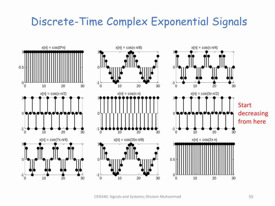
As 𝜔0 is gradually increased, the rate of oscillations in the discrete-time signal

does not keep on increasing. If 𝜔0 is increased from 0 to 2𝜋, the rate of

oscillations first increase and then decreases.

Note in particular that for 𝜔0 = 𝜋 or for any odd multiple of 𝜋,

𝑒𝑗𝜋𝑛 = 𝑒𝑗𝜋𝑛= −1 𝑛

so that the signal oscillates rapidly, changing sign at each point in time.



0 10 20 300

0.5

1x[n] = cos(0*n)

0 10 20 30-1

0

1x[n] = cos( n/8)

0 10 20 30-1

0

1x[n] = cos( n/4)

0 10 20 30-1

0

1x[n] = cos( n/2)

0 10 20 30-1

0

1x[n] = cos( n)

0 10 20 30-1

0

1x[n] = cos(3 n/2)

0 10 20 30-1

0

1x[n] = cos(7 n/4)

0 10 20 30-1

0

1x[n] = cos(15 n/8)

0 10 20 300

0.5

1x[n] = cos(2 n)

Start decreasing from here


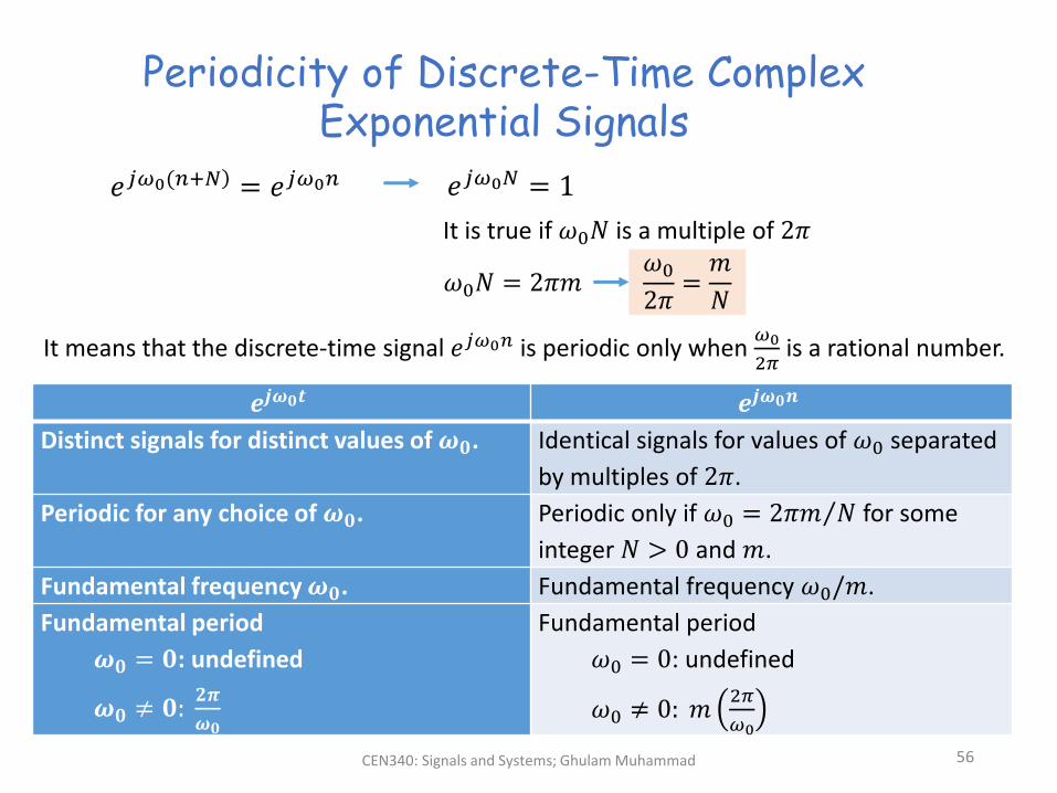
Periodicity of Discrete-Time Complex Exponential Signals

𝑒 ሻ𝑗𝜔0(𝑛+𝑁 = 𝑒𝑗𝜔0𝑛 𝑒𝑗𝜔0𝑁 = 1

It is true if 𝜔0𝑁 is a multiple of 2𝜋

𝜔0𝑁 = 2𝜋𝑚𝜔0

2𝜋=𝑚

𝑁

It means that the discrete-time signal 𝑒𝑗𝜔0𝑛 is periodic only when 𝜔0

2𝜋is a rational number.

𝒆𝒋𝝎𝟎𝒕 𝒆𝒋𝝎𝟎𝒏

Distinct signals for distinct values of 𝝎𝟎. Identical signals for values of 𝜔0 separated

by multiples of 2𝜋.

Periodic for any choice of 𝝎𝟎. Periodic only if 𝜔0 = Τ2𝜋𝑚 𝑁 for some

integer 𝑁 > 0 and 𝑚.

Fundamental frequency 𝝎𝟎. Fundamental frequency 𝜔0/𝑚.

Fundamental period

𝝎𝟎 = 𝟎: undefined

𝝎𝟎 ≠ 𝟎:𝟐𝝅

𝝎𝟎

Fundamental period

𝜔0 = 0: undefined

𝜔0 ≠ 0: 𝑚2𝜋

𝜔0


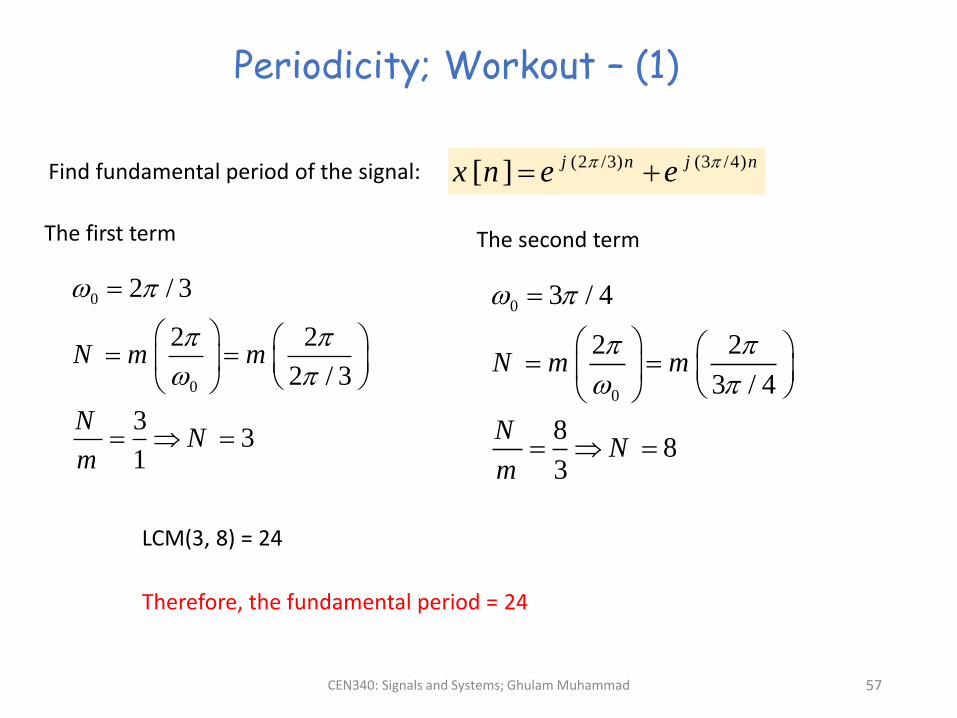
Periodicity; Workout – (1)

Find fundamental period of the signal: (2 /3) (3 /4)[ ] j n j nx n e e

The first term

0

0

2 / 3

2 2

2 / 3

33

1

N m m

NN

m

0

0

3 / 4

2 2

3 / 4

88

3

N m m

NN

m

LCM(3, 8) = 24

Therefore, the fundamental period = 24

The second term


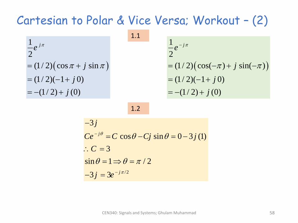
Cartesian to Polar & Vice Versa; Workout – (2)

1

2

(1/ 2) cos sin

(1/ 2)( 1 0)

(1/ 2) (0)

je

j

j

j

1

2

(1/ 2) cos( ) sin( )

(1/ 2)( 1 0)

(1/ 2) (0)

je

j

j

j

/2

3

cos sin 0 3 (1)

3

sin 1 / 2

3 3

j

j

j

Ce C Cj j

C

j e

1.1

1.2


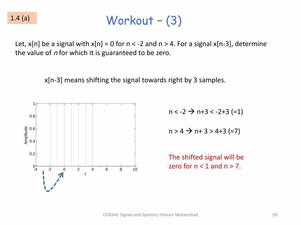
Workout – (3)

Let, x[n] be a signal with x[n] = 0 for n < -2 and n > 4. For a signal x[n-3], determine the value of n for which it is guaranteed to be zero.

x[n-3] means shifting the signal towards right by 3 samples.

-4 -2 0 2 4 6 8 100

0.2

0.4

0.6

0.8

1

t

Am

plit

ud

e

n < -2 n+3 < -2+3 (=1)

n > 4 n+ 3 > 4+3 (=7)

The shifted signal will be zero for n < 1 and n > 7.

1.4 (a)


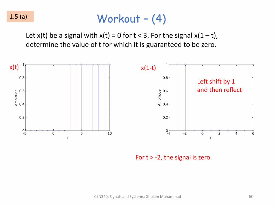
Workout – (4)

Let x(t) be a signal with x(t) = 0 for t < 3. For the signal x(1 – t), determine the value of t for which it is guaranteed to be zero.

-5 0 5 100

0.2

0.4

0.6

0.8

1

t

Am

plit

ud

e

-4 -2 0 2 4 60

0.2

0.4

0.6

0.8

1

t

Am

plit

ud

e

x(t) x(1-t)

Left shift by 1 and then reflect

For t > -2, the signal is zero.

1.5 (a)

-4 -2 0 2 4 60

0.2

0.4

0.6

0.8

1

t

Am

plit

ud

e

-5 0 5 100

0.2

0.4

0.6

0.8

1

t

Am

plit

ud

e


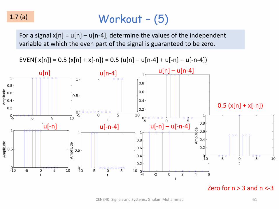
Workout – (5)

For a signal x[n] = u[n] – u[n-4], determine the values of the independent variable at which the even part of the signal is guaranteed to be zero.

EVEN{ x[n]} = 0.5 (x[n] + x[-n]) = 0.5 (u[n] – u[n-4] + u[-n] – u[-n-4])

-5 0 5 100

0.5

1

t

Am

plit

ud

e

-10 -5 0 5 100

0.5

1

t

Am

plit

ud

e

-10 -5 0 5 100

0.5

1

t

Am

plit

ud

e

-5 0 5 100

0.2

0.4

0.6

0.8

1

t

Am

plit

ud

e

-10 -5 0 5 100

0.2

0.4

0.6

0.8

1

t

Am

plit

ud

e

u[n]

u[-n]

u[n-4]

u[-n-4]

u[n] – u[n-4]

u[-n] – u[-n-4]

0.5 (x[n] + x[-n])

Zero for n > 3 and n <-3

1.7 (a)


Workout – (6)

For a signal x(t) = sin(0.5t), determine the values of the independent variable at which the even part of the signal is guaranteed to be zero.

1.7 (b)

-30 -20 -10 0 10 20 30-1

-0.5

0

0.5

1

t

Am

plit

ud

e

It is always an odd signal, so the even part is zero for all values of t.


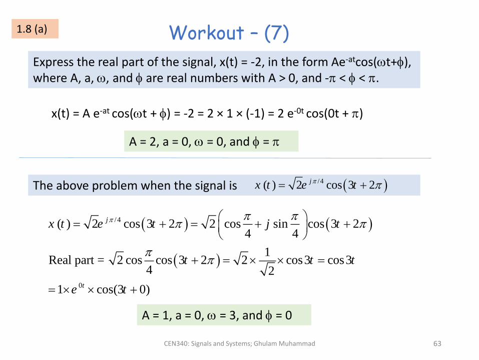
Workout – (7)

Express the real part of the signal, x(t) = -2, in the form Ae-atcos(t+), where A, a, , and are real numbers with A > 0, and - < < .

1.8 (a)

x(t) = A e-at cos(t + ) = -2 = 2 × 1 × (-1) = 2 e-0t cos(0t + )

A = 2, a = 0, = 0, and =

The above problem when the signal is /4( ) 2 cos 3 2jx t e t

/4

0

( ) 2 cos 3 2 2 cos sin cos 3 24 4

1Real part = 2 cos cos 3 2 2 cos3 cos3

4 2

1 cos(3 0)

j

t

x t e t j t

t t t

e t

A = 1, a = 0, = 3, and = 0


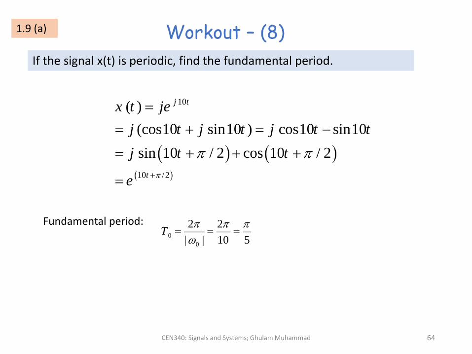
Workout – (8)

If the signal x(t) is periodic, find the fundamental period.

10

10 /2

( )

(cos10 sin10 ) cos10 sin10

sin 10 / 2 cos 10 / 2

j t

t

x t je

j t j t j t t

j t t

e

Fundamental period:0

0

2 2

| | 10 5T

1.9 (a)


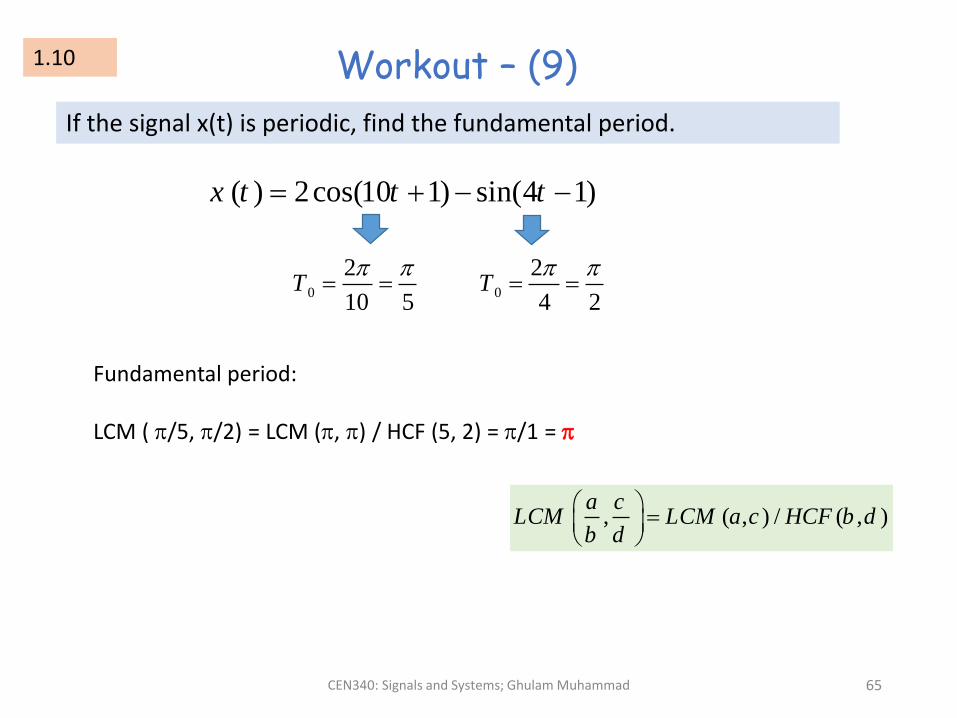
Workout – (9)

If the signal x(t) is periodic, find the fundamental period.

1.10

( ) 2cos(10 1) sin(4 1)x t t t

0

2

10 5T

0

2

4 2T

Fundamental period:

LCM ( /5, /2) = LCM (, ) / HCF (5, 2) = /1 =

, ( , ) / ( , )a c

LCM LCM a c HCF b db d


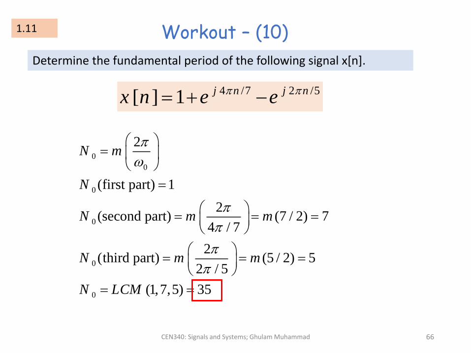
Workout – (10)

Determine the fundamental period of the following signal x[n].

1.11

4 /7 2 /5[ ] 1 j n j nx n e e

0

0

0

0

0

0

2

(first part) 1

2(second part) (7 / 2) 7

4 / 7

2(third part) (5 / 2) 5

2 / 5

(1,7,5) 35

N m

N

N m m

N m m

N LCM


Acknowledgement

The slides are prepared based on the following textbook:

• Alan V. Oppenheim, Alan S. Willsky, with S. Hamid Nawab, Signals & Systems, 2nd Edition, Prentice-Hall, Inc., 1997.

Special thanks to

• Prof. Anwar M. Mirza, former faculty member, College of Computer and Information Sciences, King Saud University

• Dr. Abdul Wadood Abdul Waheed, faculty member, College of Computer and Information Sciences, King Saud University

Documents

Signals and Systems: IntroductionCEN340: Signals and Systems; Ghulam Muhammad 18 1.2 Transformations of the Independent Variable The transformationofasignalis one of the central concepts