Signature of chaos in the semi quantum behavior of a ... · mental physics, nuclear physics and quantum chemistry as well. The definition and observation of chaotic be-havior in classical

Vol.2, No.3, 145-154 (2010) Natural Science http://dx.doi.org/10.4236/ns.2010.23024

Copyright © 2010 SciRes. OPEN ACCESS

Signature of chaos in the semi quantum behavior of a classically regular triple well heterostructure

Tiokeng Olivier Lekeufack1, Serge Bruno Yamgoue2, Timoleon Crepin Kofane1,3

1Laboratory of Mechanics, Department of Physics, Faculty of Science, University of Yaounde I, Yaounde, Cameroon; [email protected] 2Department of Physics Higher, Teacher’s Training College, Bamenda, Cameroon 3The Abdus Salam International Center for Theoretical Physics, Trieste, Italy

Received 28 December 2009; revised 14 January 2010; accepted 25 January 2010.

ABSTRACT

We analyze the phenomenon of semiquantum chaos in the classically regular triple well model from classical to quantum. His dynamics is very rich because it provides areas of regular be-havior, chaotic ones and multiple quantum tun-neling depending on the energy of the system as the Planck’s constant varies from 0 to 1. The Time Dependent Variational Principle TDVP using generalized Gaussian trial wave function, which, in many-body theory leads to the Hartree Fock Approximation TDHF, is added to the tech-niques of Gaussian effective potentials and both are used to study the system. The extended classical system with fluctuation variables non- linearly coupled to the average variables exhibit energy dependent transitions between regular behavior and semi quantum chaos monitored by bifurcation diagram together with some numerical indicators.

Keywords: Nonlinear Dynamics; Semi Quantum Chaos; Effective Potential

1. INTRODUCTION

The quantum computer science, the quantal dynamics of hetero-structures, the mesoscopic behavior of some sys-tems, the chaotic entropy production in open quantum systems, the zero momentum (long wavelength) part of the problem of pair production of charged scalar parti-cles by a strong external electric field [1], the quantum suppression of diffusion (dynamic localization) [2] and the quantum unique ergodicity in statistical thermody-namics are good candidates for a wide range of the study and the application of semiquantum chaos in experi-mental physics, nuclear physics and quantum chemistry as well. The definition and observation of chaotic be-havior in classical systems are familiar and well under-

stood [3,4]. However, the proper definition of chaos for quantum systems and its experimental manifestations are still unclear [5-8]. We use the term semiquantum chaos to refer to the study of the quantum dynamics of systems whose classical limit is regular (restriction to Hamilto-nian systems).

Over the last years, different approaches of studying chaos in classical and quantum systems have attracted increasing attention. For example, we have the prob-lem of pair production of particles by strong external electric field, the two particles interaction through a biquadratic coupling, i.e., a two-degrees of freedom system of which one is classical and the other purely quantum non linearly coupled and which exhibit chaos [9-11]. In addition, great attention is focused on a sys-tem of two particles non-linearly coupled, whose clas-sical limit is chaotic, involving quantum properties. This is the case for the authors of [9], who studied the duality wave/particle to take into account the quantum dynamics, then combined Quantum Theory of Motion (QTM) with Quantum Fluid Dynamics (QFD) in clas-sical chaos, and found quantum parameters being cha-otic. For the full quantum dynamics, only experimental studies have been done up till date on hetero-structures undergoing multiple tunneling resonance, and leading to different approaches of building quantum computers [12,13]. In addition to all the aforementioned routes of analyzing non-classical chaos, many theories and for-malisms are always used. One of the most important of these routes is the time dependent variational approach, which, in the many body theory, leads to the TDHF using a Gaussian trial wave function [14-20]. The ap-pearance of this wave function has provided great and interesting results not only in general universe physics field, but also in nuclear physics and quantum chemis-try [14,16]. This usage generally integrates the mean field theory [21-24]. The signature of the Gaussian Effective potential GEP [1,17,25,26] is also a good indicator of non-classical chaos. In fact, effective po-tentials [26] are used to assess the impact of quantum

mailto:[email protected]�

T. O. Lekeufack et al. / Natural Science 2 (2010) 145-154


146

effects such as zero point fluctuation and tunneling on the magnitude and the geometry of classical potentials for which they are an extension because carrying quantum corrections. Since some of the diagnostics [17,27,28] for chaos are based on the geometry of the potential, the effective potential techniques are espe-cially powerful in combination with such method.

Our aim in this paper is to study the semiquantal dy-namics of a triple-well potential hetero－structure. We introduce additional (fluctuation) degrees of freedom at order of the Planck’s constant, representing quantum counterpart. The non-linear coupled system of the first order autonomous flow is obtained and both analytically and numerically studied. The complete dynamics of the coupled quantum and classical oscillators is described by a classical effective Hamiltonian, which is the expecta-tion value of the quantum Hamiltonian or equivalently the Dirac’s action. The utilization of the (GEP) to draw the scheme of the system evolution provides fixed points, tunneling and multiple resonant. The numerical simula-tions are sometimes in good agreement, and bear some-what surprises.

Our paper is organized as follows: in Section 2, we briefly describe our model of triple-well hetero-structure and apply the time dependent variational principle from which we obtain our basic set of equations. Sec-tion 3 presents some analytical considerations and in-troduces the GEP. Section 4 contains numerical simu-lations to confirm assumptions made earlier in the previous sections. Finally, Section 5 summarizes the main results of the paper and provides discussion with perspectives for future works.

2. MODEL AND EQUATIONS

This section is to describe the triple-well hetero-structure model and draw the basic set of motions equations. Het-ero-structures, besides offering very interesting new technological perspectives, represent a unique opportu-nity to study fundamental question of mechanics such as many-body interaction, resonant tunneling, ergodicity and chaos [29-31]. A triple quantum well structure TQWS, all like a double quantum well structure DQWS constructed by the authors of the reference [13], can be constructed under several practical apparatus with GaAs/ AlGaAs. Physically, the structure presents the diagram of a tri-stable potential energy, which is the potential energy including stable and unstable equilibrium posi-tions:

2 4 6( )2! 4! 6!

A B CV Q Q Q Q (1)

where Q is the coordinate and ( )V Q the potential en-

ergy; A , B , and C are physical parameters on which depends the numerous variety of configurations. This type of potential is called 6 potential and exhibits several configurations according to the values of the

constants A, B, and C. On the one hand, we can have mono- and bi-stable catastrophic potentials i.e. one and two potential wells, respectively. It corresponds to cases of beams, flexible or breakable structures. On the other hand, we have mono-, bi- and tri-stable non-catastrophic configurations, and it corresponds for example to the potentials of O-H chemical bound in ice. It can also de-scribe the dynamics of some rigid structures, oscillators, hetero structures as well. We focus our attention on triple well configuration in order to study its various usages, to find out the importance and the rich dynamics offered by the additive potential well considering its symmetry. Note that more extensive works have recently been done

on the 6 potential [32-34] and good results were ob-tained about its higher precisions brought in the study of the various systems described by it. The graph of Fig-ure.1 shows the potential energy. Our case belongs to mesoscopic physics, which deals with systems that are macroscopic but retain essential quantum features [30].

Consider a particle submitted to that potential energy. The classical action is given by:

QVt

QdtS

2

2

1 (2)

From this action, we can derive the Lagrangian and through the Euler-Lagrange equations with respect to the coordinates, we come out with the first order autono-mous system flow. This is the classical approach of our problem. It is obvious to realize, by solving the Sch- rödinger equation, that the corresponding quantum dy-namics looks regular no matter whether this classical system behaves regularly or not:

tQQVdQ

dtQ

ti ;

2

1;

2

2

(3)

As explained in the introduction, it is quite an interesting and difficult approach to find whether our system bears quantum features or not. It corresponds to a situation where a classical oscillator interacts with quantum one through bi-cubic non-linear coupling. This necessitates the introduction of additive degrees of freedom, namely

Figure 1. The triple well oscillator potential, Eq.1 with A=1.0; B=0.0706 and C=0.0034.



147

fluctuation ones. Their quantum nature belongs to the significance of the Planck’s constant . We introduce classical and quantum coordinates [18]

Qtq ; 22 QQtG (4)

Together with classical and quantum momenta [18]

Pt ;

Q

itp (5)

The < > has the sense of the mean value. We now consider a trial wave function, particularly the one that has been successfully introduced by Gauss [15,18,35] and whose results were in good convenience with the physics of the considered system

qQP

iqQNtQ

2

2

1exp, (6)

With 112

2G t i t from the authors of [15].

This wave function has to satisfy usual quantum re-quirements such as the normalization condition and the Heisenberg uncertainty principle. The normalization condition gives 4

12 GN and the mean values are

easily calculated

Q q t ; i p tQ

;

2 2Q q G t ; i pq Gt

Moreover, the uncertainty principle is obtained:

2

1

212

12

1212222 4

4

1

GGGPPQQ

2

412

21

2 G

Q , P , G and are variational parameters and

we demand that their variation vanishes at infinity. We now turn to the derivation of appropriate semi

quantum equations of motion. The TDHF or Gaussian variational approximation can easily be performed with the help of Dirac’s variational principle [15]. We require the effective action

tHt

itdtS eff (7)

to be stationary against arbitrary variation of a nor-malized wave function which vanishes at t :

0Seff

for all , with 1 . This is equ-

ivalent to the exact time dependent Schrödinger equation. With this variational principle, one can solve the quan-tum mechanical time evolution problem approximately by restricting the variation of the wave function to a sub space of Hilbert space. The effective action is therefore given by:

qVG

GHqpdtS cleff

22

2

12

8

qVG

qVG 6

334

22

488

(8)

where

qVp

pqH cl 2

,2

; n

nn

Q

VV

(9)

This contains higher order additive term in 33G symbolizing higher quantum correction as compared to Eq.6 of [18] and Eq.18 of [35]. The appearance of the additive term may increase the richness of the studied systems dynamics. The semi quantum variational equa-tions of motion are therefore derived via the Euler La-grange equation for the effective action, Eq.9, by inde-pendent variation with respect to Q , P , G and :

qVG

qVG

qVG

GG

qVG

qVG

qVp

pq

622

4222

522

3

1642

12

8

1

4

162

(10)

As compared to Eq.7 of [18] and Eqs.22-25 of [35], there appear additive non-linear terms. We expect more corrections on the dynamics of the aforementioned stud-ied system. The above equations are the TDHF ones because using the Gaussian wave function in Dirac’s principle. The validity of this TDHF approximation, which has been widely tested [11,18] by being applied to various quantum mechanical problems and drawing good results, is awaited here. Since the equations are highly nonlinear, we expect the trajectories to be regular and irregular providing chaotic behavior. It is important to note that our equations are coupled, showing the link between classical and quantum interactions. At 0 classical limit, only the first two equations remain, con-firming that the fluctuation variables are responsible for quantum effects. In addition, the Ehrenfest theorem is then verified to confirm the validity of our system [17]. 3. GEP AND THEORETICAL ANALYSIS The purpose of this section is to derive the Gaussian Effective Potential (GEP) and to report some analytical considerations, which may help to better understand the dynamics of the semiquantum equations of motion.

3.1. The Static GEP

The variety of techniques used to study dynamical sys-tems comes about because the measures (such as K en-tropy [36], Lyapunov numbers [36-39]), the diagnostics (the Melnikov functions [38-40]), and the signatures of chaos, which generally lie in phase space, are dynamic and have no direct interpretation in quantum dynamics. We consider a parallel approach, that of using classical techniques of analysis by reducing the problem to that of an effective classical system i.e. looking at Hamiltons’ equations in a modified potential. Effective potentials are therefore used to assess the impact of quantum ef-



148

fects such as zero-point fluctuations and tunneling on the magnitude and the geometry of the classical potentials. It was introduced by Stevenson [26] and successfully tested in the Henon Heiles and four leg potentials prob-lem. Most of the diagnostics for chaos are based on the geometry of the potential. The effective potential tech-nique is especially powerful in combination with such method [17]. The idea of Stevenson is to approximate the effective potential of a system by using Gaussian wave function. In general, the effective potential of a system gives us a picture of how the quantum fluctua-tions modify the classical potential. Following the con-served total energy for our non-dissipative model with its complicated functions of q , p , G and , we

choose the simplest initial conditions with zero momenta 000 ttp ; then, evaluating the initial total energy

2

22

2 QQVE

we have:

CG

qC

BG

qC

qB

AG

GqVGqE

482824228),(

332

2242

(11)

At the minima of the classical potential, (i.e. q = 0 or q = ± 17.2, numerically), we obtain the initial energy for the correspondent minimum q = 0,

33

22

48828)( G

CG

BG

A

GGEq

(12)

which is a function of the initial value of G: this is the relevant control parameter for our model. We now derive the GEP. In analogy to a classical system, we consider the effective potential which is defined as the total minus the kinetic energy, from Eq.8, the kinetic part being zero according to the initial conditions. Thus,

qC

qB

AG

GqVGqEGqVeff 24228

,, 42

CG

qC

BG

4828

332

22

(13)

In Figure 2, we present equipotentials for the GEP corresponding to couples of (q,G) varying through

Figure2. The effective semi-quantum potential (GEP), Eq.13 restricted in the q-G positive plane.

Eq.10 for the same conservative energy. It shows how the classical potential is modified.

In the particular case of a potential well, the Heisen-berg uncertainty principle implies that, if the centroid is concentrated in a small region ΔQ then the uncertainty on the conjugate momentum ΔP is very large ΔP ≥ ћ/2ΔQ; there appears a large kinetic contribution in the total energy. In the triple well, the quantum fluctuations lower the potential barriers such that a particle with clas-sical insufficient energy to spray over the barrier finds it possible: that is quantum tunnel effect [21-24]. The most interesting features are the valleys in the potential energy surface that lead to the saddle point regions separating the three effective potential wells. They are observable at q = 10.9, corresponding to the maximum of the classical potential. The GEP, in its analytical expression, shows the quantum corrections on the classical potential. New phenomena are expected as shown in Figure 2. In some situations, this potential is shown to exhibit chaotic be-havior for some restricted energy ranges [41]. According to the graph, we expect multiple quantum tunnel effects, as well as energy (medium value) dependent transitions between regular and chaotic motion in the GEP; this needs to be confirmed in the numerical study. Quantum tunneling must be observable in our system, for energy range between the potential wells. Since the potential has symmetric wells, we expect on resonance [18] tun-neling process to occur. One can also explain this using

the static effective potential effV q that is obtained by

eliminating G in ,effV q G via. From Eq.13:

q

Cq

BA

qG

qGqVqVeff

24228

~ 42

C

qGq

CB

qG

4828

332

22

(14)

where G(q) is the solution of the following equation:

02

242

8

2

42

2422

324

CGq

Cq

BA

CGq

CB

CG

(15)

Figure 3, we realise that qVeff~ (Static GEP) changes

from qV and GqVeff , as if there were a phase transition.

Figure 3. The static effective potential.



149

3.2. Fix Points and Instabilities

Our potential shows the classical contribution plus the higher order quantum corrections. Note that the num-ber of valleys is in increase as compared to the one in [35]; so does the number of fixed points by two. This increase was earlier predicted by those authors be-cause of the higher order term corrections considered ( 33G ) in the GEP. In the fix points’ theory, a hetero structure bears additive properties whose importance is over the aim of this paper. Nevertheless, we focus on the variety of its usage while considering it. Our system offers various possibilities and useful aspects therewith into its rich dynamics (see stationary condi-tions 0 Gqp ). Concavities observed in the pic-

ture are good diagnostics for chaos [30-32]. Really, since there are various combinations of initial conditions cor-responding to the same total energy, numerically unob-servable chaos may exist at all energies. Nevertheless, it did not happen so; that is why it was difficult to find energy ranges where chaos occurred. As G increases in the GEP, three minima appear in the half plane, corre-sponding to the well minima of the original problem; two saddle points also emerge, interestingly. In addition, the pq, system, as driven by the ,G system, is like

a non-linearly driven Duffing oscillator [17,39] with back reaction. With these ingredients, added to the highly non-linearity, it is not surprising that our semi quantum equations exhibit chaos. On the other hand, the instabilities are important and their study is based on the motion equations Eq.10 in the second order form to show the similarity to coupled oscillators:

0

02

2

GG

qq

eff

eff

(16)

with

4222

2

12026

1

82q

CqC

GBC

GB

GAeff

(17)

and 2

22422

42122 G

CGq

CBq

CBqAeff

(18)

Two coupled parametric oscillators then describe the dynamic of the system. Both oscillators can become un-stable due to exponentially growing modes for a finite range of initial values for q and G. Taking the both ef-fective mass squared terms to be negative, gives the conditions

21

42

1

4 32²

²

16

45

8

2

12²

3

132²

²

16

45

8

2

12²

3

1

A

CB

Cq

C

BqGA

CB

Cq

C

Bq

(19) with the range

41

41

²

²290

²

²290

C

B

C

Aq

C

B

C

A (20)

for Eq.17; and

21

42

14 32

²

²16

3

8

2

12²

32

²

²16

3

8

2

12²

C

A

C

Bq

C

BqG

C

A

C

Bq

C

Bq

(21) with the range

41

41

²

²26

²

²26

C

B

C

Aq

C

B

C

A (22)

for Eq.18. The both ranges of q indicate the relationship among

the parameters A, B and C to be satisfied for a given po-tential in order to present oscillations with possible in-stabilities:

0²

²2

C

B

C

A that is CBA 2

² (23)

For G to remain positive, the previous conditions give

21

4

21

4

32

²

²16

45

8

2

12²0

32²

²

16

45

8

2

12²

3

10

C

A

C

Bq

C

BqG

C

AB

Cq

C

BqG

(24) Hence, the instability zone added to the q range ob-

tained from Eq.17 gives

21

4 32

²

²16

45

8

2

12²

3

10

C

A

C

Bq

C

BqG (25)

Note that our parameters satisfy the condition Eq.23 and the q range for instability is 9.10q or 9.10q ,

corresponding to domains containing the two extreme classical potential wells. We can conclude that the equi-librium positions q = 17.2 and q =17.2 of our potential are unstable ones. Nevertheless, note that condition Eq.25 provides the criterion not only for a better choice of ini-tial G, but also for sensitivity to initial conditions.

4. NUMERICAL STUDIES

In this section, we present the results obtained by direct numerical integrations of our semi quantum equations of motion. Numerical integration is necessary for us in or-der to confirm the estimates of the theoretical predictions and/or to obtain other results in domains where the GEP, and the analytical study cannot be successful. In fact, it is the principal mean that allows knowing about the ex-act behavior of the solutions for non-trivial nonlinear ordinary differential (semi quantum) equations Eq.16.

Unfortunately, unlike an analytical relation from which one can discuss the appearance of chaos for different initial conditions, the numerical integration has the draw back of requiring a discrete variation of the control pa-rameter of the system. Consequently, numerically study-ing such a semi quantum system for several values of its control parameter, which may vary within intervals of relatively long length, will demand a cumbersome quan-tity of plots. Thus, despite the fact that we focus great



150

attention only on the influence of the control parameter, the numerical description involves quite a large number of plots, where lie the key results of this paper. The fourth-order Runge - Kutta algorithm is the scheme we have used. The time step is fixed at Δt = 1e – 3. We al-ways fixed 000 ttp initially and chose G, together with various values for q to represent initial configurations corresponding to varying total energy. Generally, we did not explore the full set of all initial conditions at a given energy. This would require much more extensive numerical calculations which is beyond the scope of the present paper.

We have used five standard indicators including Bi-furcation diagrams, phase portraits, frequency spectrum, Poincare sections displays and computation of maximal Lyapunov exponent to characterize the long time dy-namics of our model under slight perturbation of initial conditions. These indicators complement each other in the following way: The bifurcation diagram indicates a range where values can be found to obtain regular or chaotic behavior; phase portraits are basically used to appreciate the shape of trajectories in the phase space on which the system evolves in time. They may be suffi-cient to state whether the dynamic is regular or not.

Nevertheless, they are not practical when the phase space is of dimension greater than two. Moreover, we cannot easily distinguish roughly between chaotic states and some quasi-periodic ones using only phase portraits. Poincare surfaces of section are useful to determine in particular the periodicity of the systems evolution. Strange attractors correspond to surfaces of section made up of an infinite number of points that occupy a bounded do-main of the cross section without forming a smooth closed curve. They may be chaotic or not. Thus, we need the maximal Lyapunov exponent to know the nature of the strange attractor, in this case. The frequency spec-trum is also useful here to determine, in particular, the value of the frequency in the case of regular periodic motion. Regular spacing shows regular motion.

For a system of first order equations of the form

,X F X t , where 1 2, ,..........T

nX X X X , the Lya-

punov exponents are defined as the asymptotic values of the eigen values of the solution of the matrix differential equation FB D X t B , assuming the initial condi-

tions nnIB 0 , where nnI is the n × n square identity

matrix. tXDF represents the Jacobean matrix of the

function F evaluated at the solution X(t). The involved Eigenvalues can be computed using the code stated by Wolf et al. [37,40].

A chaotic state is the one for which at least one expo-nent is positive. The bifurcation diagram (see Figure 4) shows here the increase of chaotic behavior of the sys-tem when moving from classical ( =0) to quantum ( =1). We present here phase portraits and correspond-

ing Poincare sections in the phase space planes of the two conjugate pairs of variable pq, and ,G for

some values of the total energy closer to the minimum of the classical potential energy. Figure 5 shows some regularity in the motion of the centroid at low energies. The first row presents the phase space at E = 4, G = 0.4 together with the corresponding frequency spectrum, which is regularly spaced; indicating regularity. Indeed, the value of the Lyapunov exponent is negative -0.0004. The remaining rows indicate the aspects of the Poincare sections in the both phase spaces for energies 0.9; 4 and 5, respectively. The motion still looks regular and pre-

Figure 4. Bifurcation diagrams as ћ moves from 0 to 1, for (a): q = 0.01, G = 0.1, (b): q = 0.01, G = 0.1, (c): q = 5.3, G = 0.09, (d): q = 17.2, G = 0.09.

Figure 5. Phase portrait and frequency spectrum in the first line for E = 4, G = 0.4; Poincaré sections in the remaining lines and from top to bottom for E = 0.9, G = 1.2; E = 4, G=1.2 and E = 5, G = 4.



151

sents a double periodicity with negative values of Lyapunov exponent. This situation is somewhat evident and the analytical studies predicted it. Once the energy keeps increasing, around the secondary minimum E = 12, G = 2.2, the motion starts to be irregular as shown in Figure 6 with multi-periodicity. The number of fixed points (five) is clearly observable at this particular state. Regular spacing starts vanishing in the frequency spec-trum; Poincare sections present separate closed curves; the Lyapunov exponent remains negative with oscilla-tions over the positive values. This is a sort of phase tran-sition. The significance of this type of motion lies on the definition of KAM tori. At E = 17, G = 10.8, there is chaos (see Figure 7) since the frequency spectrum has irregular spacing and the Lyapunov exponent is positive (not shown).

An attractor seems to appear in its limit cycle around the secondary minimum of the potential energy. However, just at E = 17.49, G = 0.39, regular motion appears once more (see Figure 8) with negative Lyapunov exponent and a four－periodic motion in Poincare sections. Around E = 18 and E = 19, strange attractor seems to appear, once more, as plotted in Figure 9. We find it strange and cha-otic since the Lyapunov exponent shifts from positive value ( + 0.224 at E = 19) to negative value (－0.0005 at E = 19.5). Regular motion is then observed at E=19.5. The particle located in the right potential well evolves regu-larly, and, chaotically sprays out from the right to the left well and remains there in highly chaotic

Figure 6. Phase portrait and Poincaré sections in the two first lines and at last, frequency spectrum with Lyapunov exponent for E = 12, G = 2.2.

Figure 7. Phase portrait and Poincaré sections for E = 17, G = 10.8.

Figure 8. Poincaré sections and Lyapunov exponent for E = 17.49, G = 0.39.



152

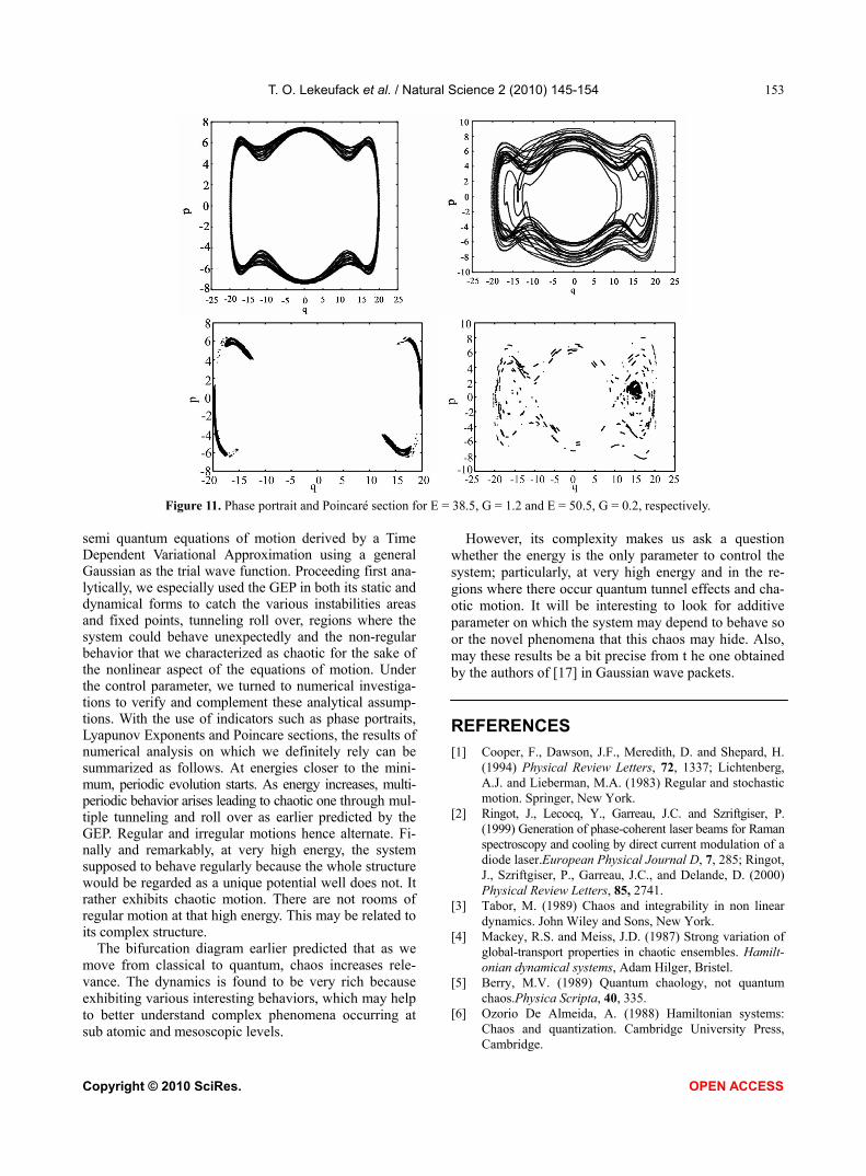
evolution as indicated in Figure 10, with Lyapunov ex-ponent equal to + 0.2295. Multiple quantum tunneling arises from E = 20 to E = 23. Between E = 25 and E = 37, chaos dominates with complicated trajectories and positive Lyapunov exponents + 0.264 and + 0.297 (not shown). At very high energy, chaos persists (see Figure 11) in its different forms of limit cycle, KAM tori or attractors. It is surprising here because, analytically, regular behavior at high energy was awaited. The energy dependent regu-

lar and chaotic behaviors hence alternate and make the dynamics very rich. 5. CONCLUSIONS In this paper, we have analyzed the dynamics of a semi quantum system that has the interesting feature of pos-sessing three potential wells. We focused our attention, in particular, on the non-linearity of the basic set of the

Figure 9. Phase portrait for E = 18, G = 0.09; E = 19, G = 4 and E = 19.5, G = 0.2, respectively and at last, Poincaré section for E = 19.5, G = 0.2.

Figure 10. Phase portrait for E = 20, G = 6.3; E = 22, G = 0.2 and E = 23, G = 0.39, respectively.



153

Figure 11. Phase portrait and Poincaré section for E = 38.5, G = 1.2 and E = 50.5, G = 0.2, respectively.

semi quantum equations of motion derived by a Time Dependent Variational Approximation using a general Gaussian as the trial wave function. Proceeding first ana-lytically, we especially used the GEP in both its static and dynamical forms to catch the various instabilities areas and fixed points, tunneling roll over, regions where the system could behave unexpectedly and the non-regular behavior that we characterized as chaotic for the sake of the nonlinear aspect of the equations of motion. Under the control parameter, we turned to numerical investiga-tions to verify and complement these analytical assump-tions. With the use of indicators such as phase portraits, Lyapunov Exponents and Poincare sections, the results of numerical analysis on which we definitely rely can be summarized as follows. At energies closer to the mini-mum, periodic evolution starts. As energy increases, multi- periodic behavior arises leading to chaotic one through mul-tiple tunneling and roll over as earlier predicted by the GEP. Regular and irregular motions hence alternate. Fi-nally and remarkably, at very high energy, the system supposed to behave regularly because the whole structure would be regarded as a unique potential well does not. It rather exhibits chaotic motion. There are not rooms of regular motion at that high energy. This may be related to its complex structure.

The bifurcation diagram earlier predicted that as we move from classical to quantum, chaos increases rele-vance. The dynamics is found to be very rich because exhibiting various interesting behaviors, which may help to better understand complex phenomena occurring at sub atomic and mesoscopic levels.

However, its complexity makes us ask a question whether the energy is the only parameter to control the system; particularly, at very high energy and in the re-gions where there occur quantum tunnel effects and cha-otic motion. It will be interesting to look for additive parameter on which the system may depend to behave so or the novel phenomena that this chaos may hide. Also, may these results be a bit precise from t he one obtained by the authors of [17] in Gaussian wave packets.

REFERENCES

[1] Cooper, F., Dawson, J.F., Meredith, D. and Shepard, H. (1994) Physical Review Letters, 72, 1337; Lichtenberg, A.J. and Lieberman, M.A. (1983) Regular and stochastic motion. Springer, New York.

[2] Ringot, J., Lecocq, Y., Garreau, J.C. and Szriftgiser, P. (1999) Generation of phase-coherent laser beams for Raman spectroscopy and cooling by direct current modulation of a diode laser.European Physical Journal D, 7, 285; Ringot, J., Szriftgiser, P., Garreau, J.C., and Delande, D. (2000) Physical Review Letters, 85, 2741.

[3] Tabor, M. (1989) Chaos and integrability in non linear dynamics. John Wiley and Sons, New York.

[4] Mackey, R.S. and Meiss, J.D. (1987) Strong variation of global-transport properties in chaotic ensembles. Hamilt- onian dynamical systems, Adam Hilger, Bristel.

[5] Berry, M.V. (1989) Quantum chaology, not quantum chaos.Physica Scripta, 40, 335.

[6] Ozorio De Almeida, A. (1988) Hamiltonian systems: Chaos and quantization. Cambridge University Press, Cambridge.



154

[7] Gutzwiller, M.C. (1990) Chaos in classical and quantum mechanics. Springer Verlag, New York.

[8] Reichl, L.E. (1992) The transition to chaos in conservative classical systems: Quantum manifestations. Springer Verlag, New York.

[9] Sengupta, S. and Chattaraj, P.K. (1996) Physics Letters A, 215, 119.

[10] Kluger, Y., Eisenberg, J.M., Svetisky, B., Cooper, F. and Mottola, E. (1991) Physical Review Letters, 67, 2427.

[11] Pradhan, T. and Khare, A.V. (1973) American Journal of Physics, 41, 59.

[12] Jona Lasinio, G., Presilla, C. and Capasso, F. (1992). Physical Review Letters, 68, 2269.

[13] Leo, K., Shah, J., Gobel, E.O., Damen, T.C., Schmitt S., Ring, Schafer, W. and Kholer, K. (1991) Physical Review Letters, 66, 201.

[14] Elze, H.T. (1995) Quantum decoherence, entropy and thermalization in strong interactions at high energy. Nuclear Physics B, 436, 213; Nuclear Physics B, 39, 169.

[15] Jackiw, R. and Kerman, A. (1978) Physics Letters A, 71, 158.

[16] Heller, E.J. (1975) Calculations and mathematical techniques in atomic and molecular physics. Journal of Chemical Physics, 62, 1544; Heller, E.J. and Sundberg, R.L. (1985) Chaotic behavior in quantum systems. Plenum Press, New York, 255.

[17] Pattanayak, A.K. and Schieve, W.C. (1994) Physical Review Letters, 72, 2855; (1992) Physical Review Letters, 46, 1821, Proceedings from workshop in honor of Sundarshan., E.G.G. Gleeson, A.M., Ed., (world scientific, Singapore, in press).

[18] Cooper, F., Pi, S.Y. and Stancioff, P.N. (1986) Physical Review D, 34, 3831.

[19] Kovner, A. and Roseinstein, B. (1983) Physical Review D, 39, 2332.

[20] Littlejohn, R.G. (1988) Physical Review Letters, 61, 2159.

[21] Tannoudji, C.C., Diu, B. and Laloe, F. (1988) Quantum mechanics, Ed., Masson.

[22] Perez, J.P. and Saint Crieq Chery, N. (1986) Relativity and Quantisation, University Paul Sabatier, Toulouse, Ed., Masson.

[23] Gaudaire, M. (1969) Propriete de la matiere: Onde et Matiere, Colorado Dunod University, Orsay.

[24] Ott, E. (1997) Chaos in dynamical systems. Cambridge University Press, Cambridge.

[25] Carlson, L. and Schieve, W.C. (1989) Physical Review A,

40, 5896. [26] Stevenson, P. (1984) Physical Review D, 30, 1712; (1985)

Physical Review D, 32, 1389. [27] Toda, M. (1974) Instability of trajectories of the lattice

with cubic nonlinearity. Physics Letters A, 48, 335. [28] Brumer, P. and Duff, J.N. (1976) Journal of Chemical

Physics, 65, 3566. [29] Capasso, F. and Datta, S. (1990) Bandgap and interface

engineering for advanced electronic and photonic devices.Physics Today, 43(2), 74.

[30] Kramer, B. (1991) Quantum coherence in mesoscopic systems. Plenum, New York.

[31] Presilla, C., Jona – Lasinio, G.. and Capasso, F. (1991) Nonlinear feedback oscillations in resonant tunneling through double barriers.Physical Review B, 43, 5200

[32] Tchoukuegno, R. and Woafo, P. (2002) Physical D 167, 86; Tchoukuegno, R., Nana, B.R. and Woafo, P. (2002) Physical Review A, 304, 362; (2003) International Journal of Non-Linear Mechanics, 38, 531.

[33] Jing, Z.J., Yang, Z.Y. and Jiang, T. (2006) Bifurcation and chaos in discrete-time predator–prey system.Chaos, Solitons and Fractals, 27, 722.

[34] Sun, Z.K., Xu, W. and Yang, X.L. (2006) Chaos, Solitons and Fractals, 27, 778.

[35] Blum, T.C. and Elze, H.T. (1996) Semiquantum chaos in the double well.Physical Review E, 53, 3123.

[36] Zaslavsky, G.M. (1985) Chaos in dynamic systems. Harwood Academic, Chur, Switzerland.

[37] Wolf, A., Swift, J. B., Swinney, H.L. and Vastano, J.A. (1985) Determining Lyapunov exponents from a time series.Physical Review D, 16, 285.

[38] Melnikov, V.K. (1963) On the stability of a center for time-periodic perturbations. Transactions of the Moscow Mathematical Society, 12, 1.

[39] Gucken, H. J. and Holmes, P. (1983) Nonlinear oscillations, dynamical systems and bifurcations of vector fields. Springer Verlag, Berlin.

[40] Yamgoue, S.B. and Kofane, T.C. (2002) The subharmonic Melnikov theory for damped and driven oscillators revisited .International Journal of Bifurcation and Chaos, 8, 1915; (2003) Chaos, Solitons & Fractals, 17, 155.

[41] Churchill, R.C., Pecelli, G. and Rod, L. (1975) J. Diff. Eqs. 17, 329; (1977) J. Diff. Eqs. 24, 329; Churchill, R.C. and Rod, D.L. (1976) Ibid. 21, 39; (1976) Ibid. 21, 66; (1980) Ibid. 37, 23.

Documents

Signature of chaos in the semi quantum behavior of a ... · mental physics, nuclear physics and quantum chemistry as well. The definition and observation of chaotic be-havior in classical