Embed Size (px)
Citation preview

Postal address: Dr.A.M.Selvam, B1 Aradhana, 42/2A Shivajinagar, Pune 411 005,
India
Signatures of Universal Characteristics of Fractal
Fluctuations in Global Mean Monthly
Temperature Anomalies
A. M. Selvam
Deputy Director (Retired)
Indian Institute of Tropical Meteorology, Pune 411 008, India
Email: [email protected]
Web sites: http://www.geocities.com/amselvam
http://amselvam.tripod.com/index.html
Running head: Universal characteristics of fractal fluctuations
Selfsimilar space-time fractal fluctuations are generic to dynamical systems in nature
such as atmospheric flows, heartbeat patterns, population dynamics, etc. The physics
of the long-range correlations intrinsic to fractal fluctuations is not yet identified. It is
important to quantify the physics underlying the irregular fractal fluctuations for
predictability studies. A general systems theory for fractals visualizes the emergence
of successively larger scale fluctuations to result from the space-time integration of
enclosed smaller scale fluctuations. The model predictions are as follows. The
probability distribution and the power spectrum for fractal fluctuations is the same
inverse power law function incorporating the golden mean. The predicted distribution
is close to the Gaussian distribution for small-scale fluctuations but exhibits fat long
tail for large-scale fluctuations with higher probability of occurrence than predicted
by Gaussian distribution. Since the power (variance i.e. square of eddy amplitude)
spectrum also represents the probability densities as in the case of quantum systems
such as the electron or photon, fractal fluctuations exhibit quantumlike chaos. The
fine structure constant for spectrum of fractal fluctuations is a function of the golden
mean and is analogous to atomic spectra equal to about 1/137. Global gridded time
series data sets of monthly mean temperatures for the period 1880 – 2007/2008 are
analysed to show that data sets and corresponding power spectra exhibit distributions
close to the model predicted inverse power law distribution. The model predicted and
observed universal spectrum for interannual variability rules out linear secular trends
in global monthly mean temperatures. Global warming results in intensification of
fluctuations of all scales and manifested immediately in high frequency fluctuations.
Key words: fractals and statistical normal distribution, power law distributions, long-
range correlations and fat tail distributions, golden mean and fractal fluctuations

1
Signatures of Universal Characteristics of Fractal
Fluctuations in Global Monthly Mean
Temperature Data
A. M. Selvam
Deputy Director (Retired)
Indian Institute of Tropical Meteorology, Pune 411 008, India
Email: [email protected]
Web sites: http://www.geocities.com/amselvam
http://amselvam.tripod.com/index.html
Selfsimilar space-time fractal fluctuations are generic to dynamical systems in nature
such as atmospheric flows, heartbeat patterns, population dynamics, etc. The physics
of the long-range correlations intrinsic to fractal fluctuations is not yet identified. It is
important to quantify the physics underlying the irregular fractal fluctuations for
predictability studies. A general systems theory for fractals visualizes the emergence
of successively larger scale fluctuations to result from the space-time integration of
enclosed smaller scale fluctuations. The model predictions are as follows. The
probability distribution and the power spectrum for fractal fluctuations is the same
inverse power law function incorporating the golden mean. The predicted distribution
is close to the Gaussian distribution for small-scale fluctuations but exhibits fat long
tail for large-scale fluctuations with higher probability of occurrence than predicted
by Gaussian distribution. Since the power (variance, i.e. square of eddy amplitude)
spectrum also represents the probability densities as in the case of quantum systems
such as the electron or photon, fractal fluctuations exhibit quantumlike chaos. The
fine structure constant for spectrum of fractal fluctuations is a function of the golden
mean and is analogous to atomic spectra equal to about 1/137. Global gridded time
series data sets of monthly mean temperatures for the period 1880 – 2007/2008 are
analysed to show that data sets and corresponding power spectra exhibit distributions
close to the model predicted inverse power law distribution. The model predicted and
observed universal spectrum for interannual variability rules out linear secular trends
in global monthly mean temperatures. Global warming results in intensification of
fluctuations of all scales and manifested immediately in high frequency fluctuations.
1. Introduction
Dynamical systems in nature such as atmospheric flows, heartbeat patterns,
population dynamics, stock market indices, DNA base A, C, G, T sequence pattern,
etc., exhibit irregular space-time fluctuations on all scales and exact quantification of
the fluctuation pattern for predictability purposes has not yet been achieved.
Traditionally, the Gaussian probability distribution is used for a broad quantification
of the data set variability in terms of the sample mean and variance. The fractal or
selfsimilar nature of space-time fluctuations was identified by Mandelbrot (1975) in
the 1970s. Representative examples of fractal fluctuations of monthly mean
temperatures for the period 1880 to 2007/2008 are shown Fig. 1.

2
Fig. 1: Representative examples of fractal fluctuations of Global gridded monthly mean
temperature anomalies for the period 1880 – 2007/2008
Fractal fluctuations (Fig. 1) show a zigzag selfsimilar pattern of successive
increase followed by decrease on all scales (space-time), for example in atmospheric
flows, cycles of increase and decrease in meteorological parameters such as wind,
temperature, etc. occur from the turbulence scale of millimeters-seconds to climate
scales of thousands of kilometers-years. The power spectra of fractal fluctuations
exhibit inverse power law of the form f-α
where f is the frequency and α is a constant.
Inverse power law for power spectra indicate long-range space-time correlations or

3
scale invariance for the scale range for which α is a constant, i.e., the amplitudes of
the eddy fluctuations in this scale range are a function of the scale factor α alone. In
general the value of α is different for different scale ranges indicating multifractal
structure for the fluctuations. The long-range space-time correlations exhibited by
dynamical systems are identified as self-organized criticality (Bak et al., 1988;
Schroeder, 1990). The physics of self-organized criticality is not yet identified. The
physics of fractal fluctuations generic to dynamical systems in nature is not yet
identified and traditional statistical, mathematical theories do not provide adequate
tools for identification and quantitative description of the observed universal
properties of fractal structures observed in all fields of science and other areas of
human interest. A recently developed general systems theory for fractal space-time
fluctuations (Selvam, 1990, 2005, 2007; Selvam and Fadnavis, 1998) shows that the
larger scale fluctuation can be visualized to emerge from the space-time averaging of
enclosed small scale fluctuations, thereby generating a hierarchy of selfsimilar
fluctuations manifested as the observed eddy continuum in power spectral analyses of
fractal fluctuations. Such a concept results in inverse power law form incorporating
the golden mean τ for the space-time fluctuation pattern and also for the power spectra
of the fluctuations (Sec. 3). The predicted distribution is close to the Gaussian
distribution for small-scale fluctuations, but exhibits fat long tail for large-scale
fluctuations. Analyses of extensive data sets of Global gridded data sets of monthly
mean temperatures for the period 1880 – 2007/2008 show that the space/time data sets
follow closely, but not exactly the statistical normal distribution, particularly in the
region of normalized deviations t greater than 2, the t values being computed as equal
to (x-av)/sd where av and sd denote respectively the mean and standard deviation of
the variable x. The general systems theory, originally developed for turbulent fluid
flows, provides universal quantification of physics underlying fractal fluctuations and
is applicable to all dynamical systems in nature independent of its physical, chemical,
electrical, or any other intrinsic characteristic. In the following, Sec. 2 gives a
summary of traditional statistical and mathematical theories/techniques used for
analysis and quantification of space-time fluctuation data sets. The general systems
theory for fractal space-time fluctuations is described in Sec. 3. Sec. 4 deals with data
and analyses techniques. Discussion and conclusions of results are presented in Sec.
5.
2. Statistical methods for data analysis
Dynamical systems such as atmospheric flows, stock markets, heartbeat patterns,
population growth, traffic flows, etc., exhibit irregular space-time fluctuation patterns.
Quantification of the space-time fluctuation pattern will help predictability studies, in
particular for events which affect day-to-day human life such as extreme weather
events, stock market crashes, traffic jams, etc. The analysis of data sets and broad
quantification in terms of probabilities belongs to the field of statistics. Early attempts
resulted in identification of the following two quantitative (mathematical)
distributions which approximately fit data sets from a wide range of scientific and
other disciplines of study. The first is the well known statistical normal distribution
and the second is the power law distribution associated with the recently identified
‘fractals’ or selfsimilar characteristic of data sets in general. In the following, a
summary is given of the history and merits of the two distributions.

4
2.1 Statistical normal distribution
Historically, our present day methods of handling experimental data have their roots
about four hundred years ago. At that time scientists began to calculate the odds in
gambling games. From those studies emerged the theory of probability and
subsequently the theory of statistics. These new statistical ideas suggested a different
and more powerful experimental approach. The basic idea was that in some
experiments random errors would make the value measured a bit higher and in other
experiments random errors would make the value measured a bit lower. Combining
these values by computing the average of the different experimental results would
make the errors cancel and the average would be closer to the "right" value than the
result of any one experiment (Liebovitch and Scheurle, 2000).
Abraham de Moivre, an 18th century statistician and consultant to gamblers made
the first recorded discovery of the normal curve of error (or the bell curve because of
its shape) in 1733. The normal distribution is the limiting case of the binomial
distribution resulting from random operations such as flipping coins or rolling dice.
Serious interest in the distribution of errors on the part of mathematicians such as
Laplace and Gauss awaited the early nineteenth century when astronomers found the
bell curve to be a useful tool to take into consideration the errors they made in their
observations of the orbits of the planets (Goertzel and Fashing, 1981, 1986). The
importance of the normal curve stems primarily from the fact that the distributions of
many natural phenomena are at least approximately normally distributed. This normal
distribution concept has molded how we analyze experimental data over the last two
hundred years. We have come to think of data as having values most of which are
near an average value, with a few values that are smaller, and a few that are larger.
The probability density function PDF(x) is the probability that any measurement has a
value between x and x + dx. We suppose that the PDF of the data has a normal
distribution. Most quantitative research involves the use of statistical methods
presuming independence among data points and Gaussian ‘normal’ distributions
(Andriani and McKelvey, 2007). The Gaussian distribution is reliably characterized
by its stable mean and finite variance (Greene, 2002). Normal distributions place a
trivial amount of probability far from the mean and hence the mean is representative
of most observations. Even the largest deviations, which are exceptionally rare, are
still only about a factor of two from the mean in either direction and are well
characterized by quoting a simple standard deviation (Clauset, Shalizi, and Newman,
2007). However, apparently rare real life catastrophic events such as major earth
quakes, stock market crashes, heavy rainfall events, etc., occur more frequently than
indicated by the normal curve, i.e., they exhibit a probability distribution with a fat
tail. Fat tails indicate a power law pattern and interdependence. The “tails” of a
power-law curve — the regions to either side that correspond to large fluctuations —
fall off very slowly in comparison with those of the bell curve (Buchanan, 2004). The
normal distribution is therefore an inadequate model for extreme departures from the
mean.
The following references are cited by Goertzel and Fashing (1981, 1986) to show
that the bell curve is an empirical model without supporting theoretical basis: (i)
Modern texts usually recognize that there is no theoretical justification for the use of
the normal curve, but justify using it as a convenience (Cronbach, 1970). (ii) The bell
curve came to be generally accepted, as M. Lippmnan remarked to Poincare (Bradley,
1969), because "...the experimenters fancy that it is a theorem in mathematics and the
mathematicians that it is an experimental fact”. (iii) Karl Pearson (best known today
for the invention of the product-moment correlation coefficient) used his newly

5
developed Chi Square test to check how closely a number of empirical distributions
of supposedly random errors fitted the bell curve. He found that many of the
distributions that had been cited in the literature as fitting the normal curve were
actually significantly different from it, and concluded that "the normal curve of error
possesses no special fitness for describing errors or deviations such as arise either in
observing practice or in nature" (Pearson, 1900).
2.2 Fractal fluctuations and statistical analysis
Fractals are the latest development in statistics. The space-time fluctuation pattern in
dynamical systems was shown to have a selfsimilar or fractal structure in the 1970s
(Mandelbrot, 1975). The larger scale fluctuation consists of smaller scale fluctuations
identical in shape to the larger scale. An appreciation of the properties of fractals is
changing the most basic ways we analyze and interpret data from experiments and is
leading to new insights into understanding physical, chemical, biological,
psychological, and social systems. Fractal systems extend over many scales and so
cannot be characterized by a single characteristic average number (Liebovitch and
Scheurle, 2000). Further, the selfsimilar fluctuations imply long-range space-time
correlations or interdependence. Therefore, the Gaussian distribution will not be
applicable for description of fractal data sets. However, the bell curve still continues
to be used for approximate quantitative characterization of data which are now
identified as fractal space-time fluctuations.
2.2.1 Power laws and fat tails
Fractals conform to power laws. A power law is a relationship in which one quantity
A is proportional to another B taken to some power n; that is, A~Bn (Buchanan, 2004).
One of the oldest scaling laws in geophysics is the Omori law (Omori, 1895). This
law describes the temporal distribution of the number of after-shocks, which occur
after a larger earthquake (i.e., main-shock) by a scaling relationship. Richardson
(1960) came close to the concept of fractals when he noted that the estimated length
of an irregular coastline scales with the length of the measuring unit. Andriani and
McKelvey (2007) have given exhaustive references to earliest known work on power
law relationships summarized as follows. Pareto (1897) first noticed power laws and
fat tails in economics. Cities follow a power law when ranked by population
(Auerbach, 1913). Dynamics of earthquakes follow power law (Gutenberg and
Richter, 1944) and Zipf (1949) found that a power law applies to word frequencies
(Estoup (1916), had earlier found a similar relationship). Mandelbrot (1963)
rediscovered them in the 20th century, spurring a small wave of interest in finance
(Fama, 1965; Montroll and Shlesinger, 1984). However, the rise of the ‘standard’
model (Gaussian) of efficient markets, sent power law models into obscurity. This
lasted until the 1990s, when the occurrence of catastrophic events, such as the 1987
and 1998 financial crashes, that were difficult to explain with the ‘standard’ models
(Bouchaud et al., 1998), re-kindled the fractal model (Mandelbrot and Hudson, 2004).
Sornette (1995) cites the works of Mandelbrot (1983), Aharony and Feder (1989)
and Riste and Sherrington (1991) and states that observation that many natural
phenomena have size distributions that are power laws, has been taken as a
fundamental indication of an underlying self-similarity. A power law distribution
indicates the absence of a characteristic size and as a consequence that there is no
upper limit on the size of events. The largest events of a power law distribution
completely dominate the underlying physical process; for instance, fluid-driven
erosion is dominated by the largest floods and most deformation at plate boundaries

6
takes place through the agency of the largest earthquakes. It is a matter of debate
whether power law distributions, which are valid descriptions of the numerous small
and intermediate events, can be extrapolated to large events; the largest events are,
almost by definition, undersampled.
A power law world is dominated by extreme events ignored in a Gaussian-world.
In fact, the fat tails of power law distributions make large extreme events orders-of-
magnitude more likely. Theories explaining power laws are also scale-free. This is to
say, the same explanation (theory) applies at all levels of analysis (Andriani and
McKelvey, 2007).
2.2.2 Scale-free theory for power laws with fat, long tails
A scale-free theory for the observed fractal fluctuations in atmospheric flows shows
that the observed long-range spatiotemporal correlations are intrinsic to quantumlike
chaos governing fluid flows. The model concepts are independent of the exact details
such as the chemical, physical, physiological and other properties of the dynamical
system and therefore provide a general systems theory applicable to all real world and
computed dynamical systems in nature (Selvam, 1998, 1999, 2001a, b, 2002a, b,
2004, 2005, 2007; Selvam et al., 2000). The model is based on the concept that the
irregular fractal fluctuations may be visualized to result from the superimposition of
an eddy continuum, i.e., a hierarchy of eddy circulations generated at each level by
the space-time integration of enclosed small-scale eddy fluctuations. Such a concept
of space-time fluctuation averaged distributions should follow statistical normal
distribution according to Central Limit Theorem in traditional Statistical theory
(Ruhla, 1992). Also, traditional statistical/mathematical theory predicts that the
Gaussian, its Fourier transform and therefore Fourier transform associated power
spectrum are the same distributions. The Fourier transform of normal distribution is
essentially a normal distribution. A power spectrum is based on the Fourier transform,
which expresses the relationship between time (space) domain and frequency domain
description of any physical process (Phillips, 2005; Riley, Hobson and Bence, 2006).
However, the model (Sec. 3) visualises the eddy growth process in successive stages
of unit length-step growth with ordered two-way energy feedback between the larger
and smaller scale eddies and derives a power law probability distribution P which is
close to the Gaussian for small deviations and gives the observed fat, long tail for
large fluctuations. Further, the model predicts the power spectrum of the eddy
continuum also to follow the power law probability distribution P.
In summary, the model predicts the following:
• The eddy continuum consists of an overall logarithmic spiral trajectory with
the quasiperiodic Penrose tiling pattern for the internal structure.
• The successively larger eddy space-time scales follow the Fibonacci number
series.
• The probability distribution P of fractal domains for the nth
step of eddy
growth is equal to τ-4n where τ is the golden mean equal to (1+√5)/2 (≈1.618).
The eddy growth step n represents the normalized deviation t in traditional
statistical theory. The normalized deviation t represents the departure of the
variable from the mean in terms of the standard deviation of the distribution
assumed to follow normal distribution characteristics for many real world
space-time events. There is progressive decrease in the probability of
occurrence of events with increase in corresponding normalized deviation t.
Space-time events with normalized deviation t greater than 2 occur with a
probability of 5 percent or less and may be categorized as extreme events

7
associated in general with widespread (space-time) damage and loss. The
model predicted probability distribution P is close to the statistical normal
distribution for t values less than 2 and greater than normal distribution for t
more than 2, thereby giving a fat, long tail. There is non-zero probability of
occurrence of very large events.
• The inverse of probability distribution P, namely, τ4n represents the relative
eddy energy flux in the large eddy fractal (small scale fine structure) domain.
There is progressive decrease in the probability of occurrence of successive
stages of eddy growth associated with progressively larger domains of fractal
(small scale fine structure) eddy energy flux and at sufficiently large growth
stage trigger catastrophic extreme events such as heavy rainfall, stock market
crashes, traffic jams, etc., in real world situations.
• The power spectrum of fractal fluctuations also follows the same distribution
P as for the distribution of fractal fluctuations. The square of the eddy
amplitude (variance) represents the eddy energy and therefore the eddy
probability density P. Such a result that the additive amplitudes of eddies
when squared represent probabilities, is exhibited by the sub-atomic dynamics
of quantum systems such as the electron or proton (Maddox, 1988, 1993; Rae,
1988). Therefore fractal fluctuations are signatures of quantumlike chaos in
dynamical systems.
• The fine structure constant for spectrum of fractal fluctuations is a function of
the golden mean and is analogous to that of atomic spectra equal to about
1/137.
• The universal algorithm for self-organized criticality is expressed in terms of
the universal Feigenbaum’s constants (Feigenbaum, 1980) a and d as
da π=22 where the fractional volume intermittency of occurrence πd
contributes to the total variance 2a2 of fractal structures. The Feigenbaum’s
constants are expressed as functions of the golden mean. The probability
distribution P of fractal domains is also expressed in terms of the
Feigenbaum’s constants a and d. The details of the model are summarized in
the following section (Sec. 3).
3. A general systems theory for fractal fluctuations
The fractal space-time fluctuations of dynamical systems may be visualized to result
from the superimposition of an ensemble of eddies (sine waves), namely an eddy
continuum. The relationship between large and small eddy circulation parameters are
obtained on the basis of Townsend’s (1956) concept that large eddies are envelopes
enclosing turbulent eddy (small-scale) fluctuations (Fig. 2).

8
Fig. 2: Physical concept of eddy growth process by the self-sustaining process
of ordered energy feedback between the larger and smaller scales, the smaller
scales forming the internal circulations of larger scales. The figure shows a
uniform distribution of dominant turbulent scale eddies of length scale 2r.
Larger-eddy circulations such as ABCD form as coherent structures sustained
by the enclosed turbulent eddies.
The relationship between root mean square (r. m. s.) circulation speeds W and w*
respectively of large and turbulent eddies of respective radii R and r is then given as
2
*
2 2w
R
rW
π= (1)
The dynamical evolution of space-time fractal structures is quantified in terms of
ordered energy flow between fluctuations of all scales in Eq. (1), because the square
of the eddy circulation speed represents the eddy energy (kinetic). A hierarchical
continuum of eddies is generated by the integration of successively larger enclosed
turbulent eddy circulations. Such a concept of space-time fluctuation averaged
distributions should follow statistical normal distribution according to Central Limit
Theorem in traditional Statistical theory (Ruhla, 1992). Also, traditional
statistical/mathematical theory predicts that the Gaussian, its Fourier transform and
therefore Fourier transform associated power spectrum are the same distributions.
However, the general systems theory (Selvam, 1998, 1999, 2001a, 2001b, 2002a,
2002b, 2004, 2005, 2007; Selvam et al., 2000) visualises the eddy growth process in
successive stages of unit length-step growth with ordered two-way energy feedback
between the larger and smaller scale eddies and derives a power law probability
distribution P which is close to the Gaussian for small deviations and gives the
observed fat, long tail for large fluctuations. Further, the model predicts the power
spectrum of the eddy continuum also to follow the power law probability distribution
P. Therefore the additive amplitudes of the eddies when squared (variance), represent

9
the probability distribution similar to the subatomic dynamics of quantum systems
such as the electron or photon. Fractal fluctuations therefore exhibit quantumlike
chaos.
The above-described analogy of quantumlike mechanics for dynamical systems is
similar to the concept of a subquantum level of fluctuations whose space-time
organization gives rise to the observed manifestation of subatomic phenomena, i.e.,
quantum systems as order out of chaos phenomena (Grossing, 1989).
3.1 Quasicrystalline structure of the eddy continuum
The turbulent eddy circulation speed and radius increase with the progressive growth
of the large eddy (Selvam, 1990, 2007). The successively larger turbulent
fluctuations, which form the internal structure of the growing large eddy, may be
computed (Eq. 1) as
22
d2W
R
Rw
π=∗ (2)
During each length step growth dR, the small-scale energizing perturbation Wn at
the nth
instant generates the large-scale perturbation Wn+1 of radius R where
∑=n
RR1
d since successive length-scale doubling gives rise to R. Eq. 2 may be
written in terms of the successive turbulent circulation speeds Wn and Wn+1 as
22
1d2
nn WR
RW
π=+ (3)
The angular turning dθ inherent to eddy circulation for each length step growth is
equal to dR/R. The perturbation dR is generated by the small-scale acceleration Wn at
any instant n and therefore dR=Wn. Starting with the unit value for dR the successive
Wn, Wn+1, R, and dθ values are computed from Eq. 3 and are given in Table 1.
Table 1. The computed spatial growth of the strange-attractor design traced by the macro-scale
dynamical system of atmospheric flows as shown in Fig. 3.
R Wn dR dθ Wn+1 θ 1.000 1.000 1.000 1.000 1.254 1.000
2.000 1.254 1.254 0.627 1.985 1.627
3.254 1.985 1.985 0.610 3.186 2.237
5.239 3.186 3.186 0.608 5.121 2.845
8.425 5.121 5.121 0.608 8.234 3.453
13.546 8.234 8.234 0.608 13.239 4.061
21.780 13.239 13.239 0.608 21.286 4.669
35.019 21.286 21.286 0.608 34.225 5.277
56.305 34.225 34.225 0.608 55.029 5.885
90.530 55.029 55.029 0.608 88.479 6.493
It is seen that the successive values of the circulation speed W and radius R of the
growing turbulent eddy follow the Fibonacci mathematical number series such that
Rn+1=Rn+Rn-1 and Rn+1/Rn is equal to the golden mean τ, which is equal to [(1 + √5)/2]
≅ (1.618). Further, the successive W and R values form the geometrical progression
R0(1+τ+τ2+τ3
+τ4+ ....) where R0 is the initial value of the turbulent eddy radius.
Turbulent eddy growth from primary perturbation ORO starting from the origin O
(Fig. 3) gives rise to compensating return circulations OR1R2 on either side of ORO,

10
thereby generating the large eddy radius OR1 such that OR1/ORO=τ and
ROOR1=π/5=ROR1O. Therefore, short-range circulation balance requirements
generate successively larger circulation patterns with precise geometry that is
governed by the Fibonacci mathematical number series, which is identified as a
signature of the universal period doubling route to chaos in fluid flows, in particular
atmospheric flows. It is seen from Fig. 3 that five such successive length step growths
give successively increasing radii OR1, OR2, OR3, OR4 and OR5 tracing out one
complete vortex-roll circulation such that the scale ratio OR5/ORO is equal to τ5=11.1.
The envelope R1R2R3R4R5 (Fig. 3) of a dominant large eddy (or vortex roll) is found
to fit the logarithmic spiral R=R0ebθ
where R0=ORO, b=tan δ with δ the crossing angle
equal to π/5, and the angular turning θ for each length step growth is equal to π/5. The
successively larger eddy radii may be subdivided again in the golden mean ratio. The
internal structure of large-eddy circulations is therefore made up of balanced small-
scale circulations tracing out the well-known quasi-periodic Penrose tiling pattern
identified as the quasi-crystalline structure in condensed matter physics. A complete
description of the atmospheric flow field is given by the quasi-periodic cycles with
Fibonacci winding numbers.
3.2 Model predictions
The model predictions (Selvam, 1990, 2005, 2007; Selvam and Fadnavis, 1998) are
3.2.1 Quasiperiodic Penrose tiling pattern
Atmospheric flows trace an overall logarithmic spiral trajectory OROR1R2R3R4R5
simultaneously in clockwise and anti-clockwise directions with the quasi-periodic
Penrose tiling pattern (Steinhardt, 1997) for the internal structure shown in Fig. 3.
The spiral flow structure can be
visualized as an eddy continuum generated
by successive length step growths ORO,
OR1, OR2, OR3,….respectively equal to R1,
R2, R3,….which follow Fibonacci
mathematical series such that Rn+1=Rn+Rn-1
and Rn+1/Rn=τ where τ is the golden mean
equal to (1+√5)/2 (≈1.618). Considering a
normalized length step equal to 1 for the
last stage of eddy growth, the successively
decreasing radial length steps can be
expressed as 1, 1/τ, 1/τ2, 1/τ3
, ……The
normalized eddy continuum comprises of
fluctuation length scales 1, 1/τ, 1/τ2, ……..
The probability of occurrence is equal to
1/τ and 1/τ2 respectively for eddy length
scale 1/τ in any one or both rotational
(clockwise and anti-clockwise) directions. Eddy fluctuation length of amplitude 1/τ
has a probability of occurrence equal to 1/τ2 in both rotational directions, i.e., the
square of eddy amplitude represents the probability of occurrence in the eddy
continuum. Similar result is observed in the subatomic dynamics of quantum systems
which are visualized to consist of the superimposition of eddy fluctuations in wave
trains (eddy continuum).
Fig. 3. The quasiperiodic Penrose tiling pattern
11
3.2.2 Logarithmic spiral pattern underlying fractal fluctuations
The overall logarithmic spiral flow structure (Fig. 1) is given by the relation
zk
wW ln∗= (4)
In Eq. (4) the constant k is the steady state fractional volume dilution of large eddy by
inherent turbulent eddy fluctuations and z is the length scale ratio R/r. The constant k
is equal to 1/τ2 (≅ 0.382) and is identified as the universal constant for deterministic
chaos in fluid flows. The steady state emergence of fractal structures is therefore
equal to
2.621
≅k
(5)
In Eq. (4), W represents the standard deviation of eddy fluctuations, since W is
computed as the instantaneous r. m. s. (root mean square) eddy perturbation amplitude
with reference to the earlier step of eddy growth. For two successive stages of eddy
growth starting from primary perturbation w∗, the ratio of the standard deviations Wn+1
and Wn is given from Eq. (4) as (n+1)/n. Denoting by σ the standard deviation of eddy
fluctuations at the reference level (n=1) the standard deviations of eddy fluctuations
for successive stages of eddy growth are given as integer multiples of σ, i.e., σ, 2σ,
3σ, etc. and correspond respectively to
3,....2,1,0,deviationdardtansnormalisedlstatistica =t (6)
The conventional power spectrum plotted as the variance versus the frequency in
log-log scale will now represent the eddy probability density on logarithmic scale
versus the standard deviation of the eddy fluctuations on linear scale since the
logarithm of the eddy wavelength represents the standard deviation, i.e., the r. m. s.
value of eddy fluctuations (Eq. 4). The r. m. s. value of eddy fluctuations can be
represented in terms of statistical normal distribution as follows. A normalized
standard deviation t=0 corresponds to cumulative percentage probability density
equal to 50 for the mean value of the distribution. Since the logarithm of the
wavelength represents the r. m. s. value of eddy fluctuations the normalized standard
deviation t is defined for the eddy energy as
1log
log
50
−=T
Lt (7)
In Eq. (7) L is the time period (or wavelength) and T50 is the period up to which the
cumulative percentage contribution to total variance is equal to 50 and t = 0. LogT50
also represents the mean value for the r. m. s. eddy fluctuations and is consistent with
the concept of the mean level represented by r. m. s. eddy fluctuations. Spectra of
time series of meteorological parameters when plotted as cumulative percentage
contribution to total variance versus t have been shown to follow closely the model
predicted universal spectrum (Selvam and Fadnavis, 1998) which is identified as a
signature of quantumlike chaos.
12
3.2.3 Universal Feigenbaum’s constants and probability distribution function for
fractal fluctuations
Selvam (1993, 2007) has shown that Eq. (1) represents the universal algorithm for
deterministic chaos in dynamical systems and is expressed in terms of the universal
Feigenbaum’s (1980) constants a and d as follows. The successive length step
growths generating the eddy continuum OROR1R2R3R4R5 (Fig. 1) analogous to the
period doubling route to chaos (growth) is initiated and sustained by the turbulent
(fine scale) eddy acceleration w∗, which then propagates by the inherent property of
inertia of the medium of propagation. Therefore, the statistical parameters mean,
variance, skewness and kurtosis of the perturbation field in the medium of
propagation are given by 432 and ∗∗∗∗ ww,ww , respectively. The associated dynamics of
the perturbation field can be described by the following parameters. The perturbation
speed ∗w (motion) per second (unit time) sustained by its inertia represents the mass, 2
∗w the acceleration or force, 3
∗w the angular momentum or potential energy, and 4
∗w the spin angular momentum, since an eddy motion has an inherent curvature to its
trajectory.
It is shown that Feigenbaum’s constant a is equal to (Selvam, 1993, 2007)
11
22
RW
RWa = (8)
In Eq. (8) the subscripts 1 and 2 refer to two successive stages of eddy growth.
Feigenbaum’s constant a as defined above represents the steady state emergence of
fractional Euclidean structures. Considering dynamical eddy growth processes,
Feigenbaum’s constant a also represents the steady state fractional outward mass
dispersion rate and a2 represents the energy flux into the environment generated by
the persistent primary perturbation W1. Considering both clockwise and
counterclockwise rotations, the total energy flux into the environment is equal to 2a2.
In statistical terminology, 2a2 represents the variance of fractal structures for both
clockwise and counterclockwise rotation directions.
The probability of occurrence Ptot of fractal domain W1R1 in the total larger eddy
domain WnRn in any (irrespective of positive or negative) direction is equal to
n
nn
totRW
RWP
211 −τ==
Therefore the probability P of occurrence of fractal domain W1R1 in the total larger
eddy domain WnRn in any one direction (either positive or negative) is equal to
n
nnRW
RWP 4
2
11 −τ=
= (9)
The Feigenbaum’s constant d is shown to be equal to (Selvam, 1993, 2007)
3
1
4
1
3
2
4
2
RW
RWd = (10)

13
Eq. (10) represents the fractional volume intermittency of occurrence of fractal
structures for each length step growth. Feigenbaum’s constant d also represents the
relative spin angular momentum of the growing large eddy structures as explained
earlier.
Eq. (1) may now be written as
( ) ( )34
34
22
22
dd2
Rw
RW
Rw
RW
∗∗
π= (11)
In Eq. (11) dR equal to r represents the incremental growth in radius for each
length step growth, i.e., r relates to the earlier stage of eddy growth.
The Feigenbaum’s constant d represented by R/r is equal to
34
34
rw
RWd
∗
= (12)
For two successive stages of eddy growth
3
1
4
1
3
2
4
2
RW
RWd = (13)
From Eq. (1)
2
*
2
2
2
2
*
1
2
1
2
2
wR
rW
wR
rW
π=
π=
(14)
Therefore
2
1
2
1
2
2
R
R
W
W= (15)
Substituting in Eq. (13)
2
1
2
1
2
2
2
2
3
1
2
1
3
2
2
2
2
1
3
1
2
1
3
2
2
2
2
1
2
2
3
1
4
1
3
2
4
2
RW
RW
RW
RW
R
R
RW
RW
W
W
RW
RWd ==== (16)
The Feigenbaum’s constant d represents the scale ratio R2/R1 and the inverse of the
Feigenbaum’s constant d equal to R1/R2 represents the probability (Prob)1 of
occurrence of length scale R1 in the total fluctuation length domain R2 for the first
eddy growth step as given in the following
( ) 4
2
2
2
2
2
1
2
1
2
11
1 −τ====RW
RW
dR
RProb (17)

14
In general for the nth
eddy growth step, the probability (Prob)n of occurrence of
length scale R1 in the total fluctuation length domain Rn is given as
( ) n
nnn
nRW
RW
R
RProb
4
22
2
1
2
11 −τ=== (18)
The above equation for probability (Prob)n also represents, for the nth
eddy growth
step, the following statistical and dynamical quantities of the growing large eddy with
respect to the initial perturbation domain: (i) the statistical relative variance of fractal
structures, (ii) probability of occurrence of fractal domain in either positive or
negative direction, and (iii) the inverse of (Prob)n represents the organised fractal
(fine scale) energy flux in the overall large scale eddy domain. Large scale energy
flux therefore occurs not in bulk, but in organized internal fine scale circulation
structures identified as fractals.
Substituting the Feigenbaum’s constants a and d defined above (Eqs. 8 and 10),
Eq. (11) can be written as
da π=22 (19)
In Eq. (19) πd, the relative volume intermittency of occurrence contributes to the total
variance 2a2 of fractal structures.
In terms of eddy dynamics, the above equation states that during each length step
growth, the energy flux into the environment equal to 2a2 contributes to generate
relative spin angular momentum equal to πd of the growing fractal structures. Each
length step growth is therefore associated with a factor of 2a2 equal to 2τ
4 ( ≅
13.70820393) increase in energy flux in the associated fractal domain. Ten such
length step growths results in the formation of robust (self-sustaining) dominant
bidirectional large eddy circulation OROR1R2R3R4R5 (Fig. 1) associated with a factor
of 20a2 equal to 137.08203 increase in eddy energy flux. This non-dimensional
constant factor characterizing successive dominant eddy energy increments is
analogous to the fine structure constant ∝-1
(Ford, 1968) observed in atomic spectra,
where the spacing (energy) intervals between adjacent spectral lines is proportional to
the non-dimensional fine structure constant equal to approximately 1/137. Further, the
probability of nth
length step eddy growth is given by a-2n
(≅6.8541-n
) while the
associated increase in eddy energy flux into the environment is equal to a2n
((≅6.8541n). Extreme events occur for large number of length step growths n with
small probability of occurrence and are associated with large energy release in the
fractal domain. Each length step growth is associated with one-tenth of fine structure
constant energy increment equal to 2a2 (∝
-1/10 ≅ 13.7082) for bidirectional eddy
circulation, or equal to one-twentieth of fine structure constant energy increment
equal to a2 (∝
-1/20 ≅ 6.8541) in any one direction, i.e., positive or negative. The
energy increase between two successive eddy length step growths may be expressed
as a function of (a2)
2, i.e., proportional to the square of the fine structure constant ∝
-1.
In the spectra of many atoms, what appears with coarse observations to be a single
spectral line proves, with finer observation, to be a group of two or more closely
spaced lines. The spacing of these fine-structure lines relative to the coarse spacing in
the spectrum is proportional to the square of fine structure constant, for which reason
this combination is called the fine-structure constant. We now know that the
significance of the fine-structure constant goes beyond atomic spectra (Ford, 1968).

15
It was shown at Eq. (5) (Sec. 3.2.2) above that the steady state emergence of fractal
structures in fluid flows is equal to 1/k (=τ2) and therefore the Feigenbaum’s constant
a is equal to
2.6212 ==τ=k
a (20)
3.2.4 Universal Feigenbaum’s constants and power spectra of fractal fluctuations
The power spectra of fluctuations in fluid flows can now be quantified in terms of
universal Feigenbaum’s constant a as follows.
The normalized variance and therefore the statistical probability distribution is
represented by (from Eq. 9)
taP
2−= (21)
In Eq. (21) P is the probability density corresponding to normalized standard
deviation t. The graph of P versus t will represent the power spectrum. The slope S of
the power spectrum is equal to
Pt
PS −≈=
d
d (22)
The power spectrum therefore follows inverse power law form, the slope
decreasing with increase in t. Increase in t corresponds to large eddies (low
frequencies) and is consistent with observed decrease in slope at low frequencies in
dynamical systems.
The probability distribution of fractal fluctuations (Eq. 18) is therefore the same as
variance spectrum (Eq. 21) of fractal fluctuations.
The steady state emergence of fractal structures for each length step growth for any
one direction of rotation (either clockwise or anticlockwise) is equal to
22
2τ=
a
since the corresponding value for both direction is equal to a (Eqs. 5 and 20 ).
The emerging fractal space-time structures have moment coefficient of kurtosis
given by the fourth moment equal to
32.9356162
824
≈=τ=
τ
The moment coefficient of skewness for the fractal space-time structures is equal
to zero for the symmetric eddy circulations. Moment coefficient of kurtosis equal to 3
and moment coefficient of skewness equal to zero characterize the statistical normal
distribution. The model predicted power law distribution for fractal fluctuations is
close to the Gaussian distribution.

16
3.2.5 The power spectrum and probability distribution of fractal fluctuations are the
same
The relationship between Feigenbaum’s constant a and power spectra may also be
derived as follows.
The steady state emergence of fractal structures is equal to the Feigenbaum’s constant
a (Eqs. 5 and 20). The relative variance of fractal structure which also represents the
probability P of occurrence of bidirectional fractal domain for each length step growth
is then equal to 1/a2. The normalized variance
na2
1 will now represent the statistical
probability density for the nth
step growth according to model predicted quantumlike
mechanics for fluid flows. Model predicted probability density values P are computed
as
n
naP
4
2
1 −τ== (23)
or
tP
4−τ= (24)
In Eq. (24) t is the normalized standard deviation (Eq. 6). The model predicted P
values corresponding to normalised deviation t values less than 2 are slightly less than
the corresponding statistical normal distribution values while the P values are
noticeably larger for normalised deviation t values greater than 2 (Table 2 and Fig. 4)
and may explain the reported fat tail for probability distributions of various physical
parameters (Buchanan, 2004). The model predicted P values plotted on a linear scale
(Y-axis) shows close agreement with the corresponding statistical normal probability
values as seen in Fig.4 (left side). The model predicted P values plotted on a
logarithmic scale (Y-axis) shows fat tail distribution for normalised deviation t values
greater than 2 as seen in Fig.4 (right side).
Table 2: Model predicted and statistical normal probability density distributions
growth step normalized
deviation cumulative probability densities (%)
n t
model predicted
P = τ-4t statistical normal
distribution
1 1 14.5898 15.8655
2 2 2.1286 2.2750
3 3 0.3106 0.1350
4 4 0.0453 0.0032
5 5 0.0066 ≈ 0.0

17
Fig. 4: Comparison of statistical normal distribution and computed (theoretical) probability density
distribution. The same figure is plotted on the right side with logarithmic scale for the probability
axis (Y-axis) to show clearly that for normalized deviation t values greater than 2 the computed
probability densities are greater than the corresponding statistical normal distribution values.
4. Data and analysis
4.1 Data sets used for the study
Gridded temperature anomalies for mean temperatures obtained from the GHCN V2
(http://www.ncdc.noaa.gov/oa/climate/ghcn-monthly/index.php and
ftp://ftp.ncdc.noaa.gov/pub/data/ghcn/v2/) monthly temperature data sets for 129
years (1880 to 2008) the months January to May and for 128 years (1880 to 2008) for
the months June to December were used for the study. Details of the data set as given
in the ‘README_GRID_TEMP’ text document are as follows. GHCN homogeneity
adjusted data was the primary source for developing the gridded fields. In grid boxes
without homogeneity adjusted data, GHCN raw data was used to provide additional
coverage when possible. Each month of data consists of 2592 gridded data points
produced on a 5 X 5 degree basis for the entire globe (72 longitude X 36 latitude grid
boxes).
Gridded data for every month from January 1880 to the most recent month (May
2008 in the present study) is available. The data are temperature anomalies in degrees
Celsius. Each gridded value was multiplied by 100 and written to file as an integer.
Missing values are represented by the value -32768.
There are two options: grid_1880_YYYY.dat.gz (used in the present study), where
YYYY is the current year and the values are calculated using the first difference
method, and anom-grid-1880-current.dat.gz which uses the "anomaly" method.
The data are formatted by year, month, latitude and longitude. There are twelve
longitude grid values per line, so there are 6 lines (72/12 = 6) for each of the 36
latitude bands. Longitude values are written from 180 W to 180 E, and latitude values

18
from 90 N to 90 S. Data for each month is preceded by a label containing the month
and year of the gridded data.
for year = begyr to endyr
for month = 1 to 12
format(2i5) month,year
for ylat = 1 to 36 (85-90N,80-85N,...,80-85S,85-90S)
format(12i5) 180-175W,175-170W,...,130-125W,125-120W
format(12i5) 120-115W,175-170W,...,70-65W,65-60W
format(12i5) 60-55W,55-50W,...,10-5W,5-0W
format(12i5) 0-5E,5-10E,...,50-55E,55-60E
format(12i5) 60-65E,65-70E,...,110-115E,115-120E
format(12i5) 120-125E,125-130E,...,170-175E,175-180E
Each file has been compressed using 'gzip'. They can be uncompressed with
'WinZip' for those using Windows 95 (and above) or with 'gzip' from most UNIX
platforms. The FORTRAN utility program 'read_gridded.f' can be downloaded to
assist in extracting data of interest. This program allows the user to extract non-
missing values for selected months and write the data to an ascii output file. The
latitude and longitude of the center of each corresponding grid box accompanies each
gridded value in the output file.
We calculated these anomalies with respect to the period 1961 - 1990 using the
First Difference Method, an approach developed to maximize the use of available
station records (Peterson and Vose, 1997; Peterson et al., 1998a; Peterson et al.,
1998b). The First Difference Method involves calculating a series of calendar-month
differences in temperature between successive years of station data (FDyr = Tyr -
Tyr-1). For example, when creating a station's first difference series for mean
February temperature, we subtract the station's February 1880 temperature from the
station's February 1881 temperature to create a February 1881 first difference value.
First difference values for subsequent years are calculated in the same fashion by
subtracting the station's preceding year temperature for all available years of station
data.
For each year and month we sum the 'first difference' value of all stations located
within the appropriate 5 X 5 degree box and divide by the total number of stations in
the box to get an unweighted first difference value for each grid box. We then
calculate a cumulative sum of these gridded first difference values for all years from
1880 to 1998 to produce a time series for each grid box. The cumulative sum is
calculated for each grid box and each month of gridded first difference data
independently through time. Each grid box time series is then adjusted to create
anomalies with respect to the period 1961 - 1990.
We developed this gridded data set to produce the most accurate time series
possible. However, this required that we treat months and grid boxes independently
through time. The use of this data is most appropriate for analyzing the change in
temperature within a particular grid box, or set of grid boxes, over a span of years. If
one is more interested in analyzing temperature changes within individual years, e.g.,
the change in temperature between February and March, 1908, or between two
regions in 1908, we recommend that the GHCN station data be used directly.

19
4.2 Analyses and results
4.2.1`Frequency distribution
Each data set (month-wise temperature time series for the period 1800 to 2008 for the
months January to May and for the period 1800 to 2007 for the months June to
December) was represented as the frequency of occurrence f(i) in a suitable number n
of class intervals x(i), i=1, n covering the range of values from minimum to the
maximum in the data set. The class interval x(i) represents dataset values in the range
x(i) ± ∆x, where ∆x is a constant. The average av and standard deviation sd for the
data set is computed as
[ ]
∑
∑ ×=
n
n
if
ifixav
1
1
)(
)()(
[ ]{ }
∑
∑ ×−=
n
n
if
ifavixsd
1
1
2
)(
)()(
The normalized deviation t values for class intervals t(i) were then computed as
sd
avixit
−=
)()(
The cumulative percentage probabilities of occurrence cmax(i) and cmin(i)
corresponding to the normalized deviation t values were then computed starting
respectively from the maximum (i=n) and minimum (i=1) class interval values as
follows.
[ ]
[ ]0.100
)()(
)()()(
1
×∑ ×
∑ ×=
n
i
n
ifix
ifixicmax
[ ]
[ ]0.100
)()(
)()()(
1
1 ×∑ ×
∑ ×=
n
i
ifix
ifixicmin
The cmax and cmin distributions with respect to the normalized deviation t values
were computed for each month for all grid points including grid points which did not
have continuous time series data. The total number of grid points available for the
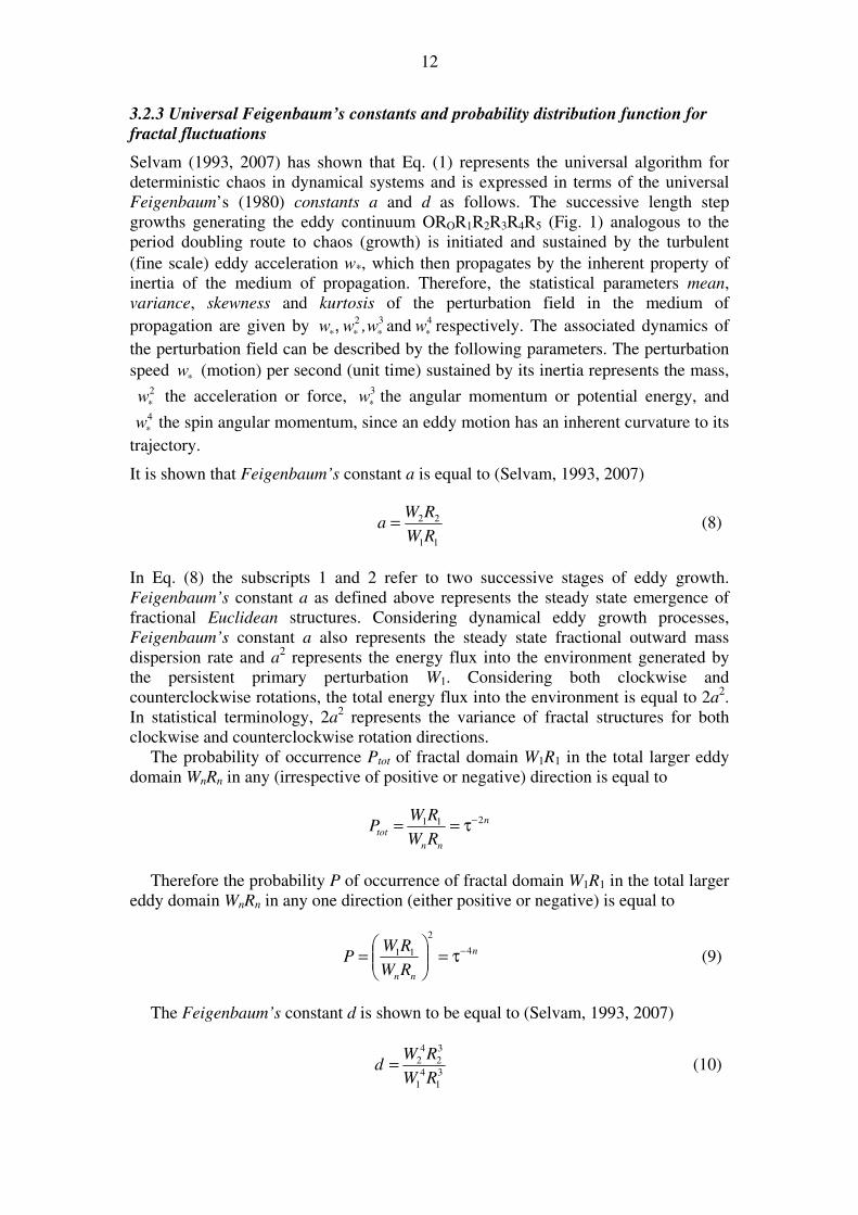
study for the months January to December is given in Fig. 5. The average and
standard deviation of cmax(i) and cmin(i) for each normalized deviation t(i) values
were then computed for each month from the corresponding distributions for all the
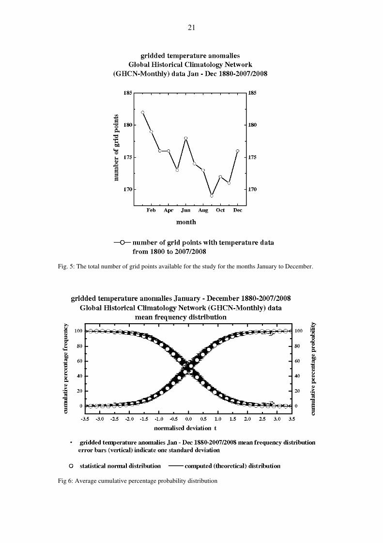
available grid points for the month. The average cumulative percentage probability
values cmax(i) and cmin(i) plotted with respect to corresponding normalized deviation
t(i) values with linear axes are shown in Fig. 6 and on logarithmic scale for the

20
probability axis in the tail region, i.e. normalized deviation t(i) values greater than 2 in
Fig. 7 for positive extremes t(i) = 2 to 4, and in Fig. 8 for negative extremes t(i) = -2
to -4. The standard deviation of each mean cmax(i) and cmin(i) value is shown as a
vertical error bar on either side of the mean in Figs. 6 to 8. The figures also contain
the statistical normal distribution and the computed theoretical distribution (Eq. 24)
for comparison. The figures show clearly the appreciable positive departure of
observed probability densities from the statistical normal distribution for extreme
values at normalised deviation t values more than 2 (Figs. 7 and 8). The observed
extreme values corresponding to t(i) values greater than 2 for cmax(i) and cmin(i)
distributions were compared for ‘goodness of fit’ with computed theoretical
distribution and statistical normal distribution as follows. For cmax(i) and cmin(i)
values, where standard deviation is available (no of observed values more than one),
if the observed distribution included the computed theoretical (statistical normal)
distribution within twice the standard deviation on either side of the mean then it was
assumed to be the same as the computed theoretical (statistical normal) distribution at
5% level of significance within measurement errors. The number of observed
distribution values which included the computed theoretical values and/or the
statistical normal distribution values within twice the standard deviation on either side
of the mean was determined. The total and percentage numbers of observed extreme
values same as computed theoretical and statistical normal distributions are given in
Fig. 9 for positive and negative tail regions (normalized deviation t greater than 2) for
the 12 months January to December. The percentage number of observed extreme
value points same as model predicted computed is more than the percentage number
of extreme value points same as statistical normal distribution for all the 12 months.
The observed distribution is closer to the model predicted theoretical than the
statistical normal distribution.
4.2.2 Continuous periodogram power spectral analyses
The power spectra of frequency distribution of monthly mean data sets were
computed accurately by an elementary, but very powerful method of analysis
developed by Jenkinson (1977) which provides a quasi-continuous form of the
classical periodogram allowing systematic allocation of the total variance and degrees
of freedom of the data series to logarithmically spaced elements of the frequency
range (0.5, 0). The cumulative percentage contribution to total variance was computed
starting from the high frequency side of the spectrum. The power spectra were plotted
as cumulative percentage contribution to total variance versus the normalized standard
deviation t equal to ( ) 1loglog 50 −TL where L is the period in years and 50T is the
period up to which the cumulative percentage contribution to total variance is equal to
50 (Eq. 7). The statistical Chi-Square test (Spiegel, 1961) was applied to determine
the ‘goodness of fit’ of variance spectra with statistical normal distribution which is
close to model predicted variance spectrum (Eqs. 21 and 24).
21
Fig. 5: The total number of grid points available for the study for the months January to December.
Fig 6: Average cumulative percentage probability distribution

22
Fig 7: Average cumulative percentage probability values on logarithmic scale for the probability axis in
the positive tail region (extreme events), i.e., normalized deviation t values greater than 2
23
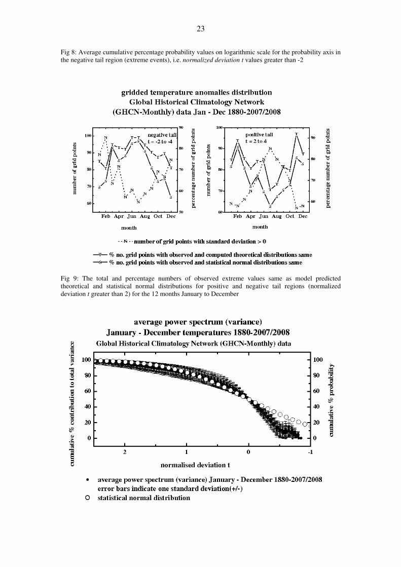
Fig 8: Average cumulative percentage probability values on logarithmic scale for the probability axis in
the negative tail region (extreme events), i.e. normalized deviation t values greater than -2
Fig 9: The total and percentage numbers of observed extreme values same as model predicted
theoretical and statistical normal distributions for positive and negative tail regions (normalized
deviation t greater than 2) for the 12 months January to December

24
Fig. 10: Average power (variance) spectrum with vertical error bars indicating one standard deviation
on either side of the mean. The statistical normal distribution is also shown in the figure for
comparison.
Fig. 11: The total number of grid points and the percentage number of grid points with variance spectra
same as statistical normal distribution.
5. Discussion and conclusions
Dynamical systems in nature exhibit selfsimilar fractal fluctuations for all space-time
scales and the corresponding power spectra follow inverse power law form signifying
long-range space-time correlations identified as self-organized criticality. The physics
of self-organized criticality is not yet identified. The Gaussian probability distribution
used widely for analysis and description of large data sets is found to significantly
underestimate the probabilities of occurrence of extreme events such as stock market
crashes, earthquakes, heavy rainfall, etc. Further, the assumptions underlying the
normal distribution such as fixed mean and standard deviation, independence of data,
are not valid for real world fractal data sets exhibiting a scale-free power law
distribution with fat tails. It is important to identify and quantify the fractal
distribution characteristics of dynamical systems for predictability studies.
A recently developed general systems theory for fractal space-time fluctuations
(Selvam, 1990, 2005, 2007; Selvam and Fadnavis, 1998) shows that the larger scale
fluctuation can be visualized to emerge from the space-time averaging of enclosed
small scale fluctuations, thereby generating a hierarchy of selfsimilar fluctuations
manifested as the observed eddy continuum in power spectral analyses of fractal
fluctuations.
The model predictions are as follows.
• The probability distribution function P of fractal fluctuations follow inverse
power law form τ-4t where τ is the golden mean, and t, the normalized

25
deviation is equal to (x-av/sd) where av and sd are respectively the average
and standard deviation of the distribution. The predicted distribution is close to
the Gaussian distribution for small-scale fluctuations (normalized deviation t
less than 2), but exhibits fat long tail for large-scale fluctuations (normalized
deviation t more than 2) with higher probability of occurrence than predicted
by Gaussian distribution. There is always a non-zero probability of occurrence
of very large amplitude, damage causing extreme events.
• The inverse of the probability distribution function, i.e. 1/P equal to τ4t
represents the domain size extent of the internal fine scale (fractal)
fluctuations of amplitude t (normalized deviation). High intensity extreme
events corresponding to t values more than 2 occur with less probability over a
larger size domain and are associated with widespread damage and loss such
as in heavy rainfall, earthquakes, traffic jams, etc.
• The power spectra of fractal fluctuations (Sec. 3) also follow inverse power
law form τ-4t and t, the normalized deviation is expressed in terms of
component periodicities L as t = {(log L/log T50)-1} where T50 is the period
upto which the cumulative percentage contribution to total variance is equal to
50. Since the power (variance, i.e., square of eddy amplitude) spectrum also
represents the probability densities as in the case of quantum systems such as
the electron or photon, fractal fluctuations exhibit quantumlike chaos.
• The precise geometry of the quasiperiodic Penrose tiling pattern underlie
fractal fluctuations tracing out robust (self-sustaining) dominant bidirectional
large eddy circulation OROR1R2R3R4R5 (Fig. 1) associated with a factor of
20a2 (20τ4) equal to 137.08203 increase in eddy energy flux. This non-
dimensional dominant eddy energy flux is analogous to and almost equal to
the fine structure constant ∝-1
of atomic spectra; the energy spacing intervals
between successive atomic spectral lines. Further, the energy increase between
two successive fine strucure eddy length step growths internal to the dominant
large eddy domain may be expressed as a function of (a2)2, i.e., proportional to
the square of the fine structure constant ∝-1
. In the spectra of many atoms,
what appears with coarse observations to be a single spectral line proves, with
finer observation, to be a group of two or more closely spaced lines. The
spacing of these fine-structure lines relative to the coarse spacing in the
spectrum is proportional to the square of fine structure constant, for which
reason this combination is called the fine-structure constant (Ford, 1968).
Analysis of historic (1880 -2008) data sets of global monthly mean temperature
(GHCN V2) time series show that the data follow closely, but not exactly the
statistical normal distribution in the region of normalized deviations t less than 2 (Fig.
6). For normalized deviations t greater than 2, the data exhibit significantly larger
probabilities as compared to the normal distribution and closer to the model predicted
probability distribution (Figs 7 and 8). A simple t test for ‘goodness of fit’ of the
extreme values (normalized deviation t > 2) of the observed distribution with model
predicted (theoretical) and also the statistical normal distribution shows that more
number of data points exhibit significant (at 5% level) ‘goodness of fit’ with the
model predicted (theoretical) distribution than with the normal distribution (Fig. 9).
The mean power spectra follow closely the statistical normal distribution for the
twelve months (Fig. 10). The power spectra mostly cover the region for normalized
deviation t less than 2 where the model predicted theoretical distribution is close to
the statistical normal distribution. A majority (more than 90%) of the power spectra
follow closely statistical normal distribution (Fig. 11) consistent with model

26
prediction of quantumlike chaos, i.e., variance or square of eddy amplitude represents
the probability distribution, a signature of quantum systems. The model predicted and
observed universal spectrum for interannual variability rules out linear secular trends
in global monthly mean temperatures. Global warming results in intensification of
fluctuations of all scales and manifested immediately in high frequency fluctuations.
The general systems theory, originally developed for turbulent fluid flows, provides
universal quantification of physics underlying fractal fluctuations and is applicable to
all dynamical systems in nature independent of its physical, chemical, electrical, or
any other intrinsic characteristic.
Acknowledgement
The author is grateful to Dr. A. S. R. Murty for encouragement during the course of
this study.
References A. Aharony and J. Feder, eds, Fractals in Physics, (North Holland, Amsterdam), Physica D 38 (1989) 1-3.
P. Andriani and B. McKelvey, Beyond Gaussian averages: Redirecting management research toward extreme
events and power laws, Journal of International Business Studies 38 (2007) 1212–1230.
F. Auerbach, Das Gesetz Der Bevolkerungskoncentration, Petermanns Geographische Mitteilungen 59 (1913) 74–
76.
P. C. Bak, C. Tang and K. Wiesenfeld, Self-organized criticality, Phys. Rev. A. 38 (1988) 364 - 374.
J. P. Bouchaud, D. Sornette, C. Walter and J. P. Aguilar, Taming large events: Optimal portfolio theory for
strongly fluctuating assets, International Journal of Theoretical and Applied Finance 1(1) (1998) 25–41.
J. V. Bradley, Distribution-free Statistical Tests, (Englewood Cliffs, Prentice-Hall, N.J., 1968).
M. Buchanan, Power laws and the new science of complexity management, Strategy and Business Issue 34 (2004)
70-79.
A. Clauset, C. R. Shalizi and M. E. J. Newman, Power-law distributions in empirical data, arXiv:0706.1062v1
[physics.data-an] 2007.
L. Cronbach, Essentials of Psychological Testing, (Harper & Row, New York, 1970).
J. B. Estoup, Gammes Stenographiques, (Institut Stenographique de France, Paris, 1916).
E. F. Fama, The behavior of stock-market prices, Journal of Business 38 (1965) 34–105.
M. J. Feigenbaum, Universal behavior in nonlinear systems, Los Alamos Sci. 1 (1980) 4-27.
K. W. Ford, Basic Physics, (Blaisdell Publishing Company, Waltham, Massachusetts, USA, 1968, p. 775)
T. Goertzel and J. Fashing, The myth of the normal curve: A theoretical critique and examination of its role in
teaching and research, Humanity and Society 5 (1981) 14-31; reprinted in Readings in Humanist Sociology,
General Hall, 1986. http://crab.rutgers.edu/~goertzel/normalcurve.htm 4/29/2007
W. H. Greene, Econometric Analysis, 5th ed. (Prentice-Hall, Englewood Cliffs, NJ, 2002).
G. Grossing, Quantum systems as order out of chaos phenomena, Il Nuovo Cimento 103B (1989) 497-510.
B. Gutenberg and R. F. Richter, Frequency of earthquakes in California, Bulletin of the Seismological Society of
America 34 (1944) 185–188.
L. S. Liebovitch and D. Scheurle, Two lessons from fractals and chaos, Complexity 5(4) (2000) 34–43.
J. Maddox, Licence to slang Copenhagen? Nature 332 (1988) 581.
J. Maddox, Can quantum theory be understood? Nature 361 (1993) 493.
B. B. Mandelbrot, The variation of certain speculative prices, Journal of Business 36 (1963) 394–419.
B. B. Mandelbrot, Les Objets Fractals: Forme, Hasard et Dimension, (Flammarion, Paris, 1975).
B. B. Mandelbrot, The Fractal Geometry of Nature, (Freeman, New York, 1983).
B. B. Mandelbrot and R. L. Hudson, The (Mis)Behavior of Markets: A Fractal View of Risk, Ruin and Reward,
(Profile, London, 2004).
E. Montroll and M. Shlesinger, On the wonderful world of random walks, in J. L. Lebowitz and E. W. Montroll
(eds.) Nonequilibrium Phenomena II, from Stochastic to Hydrodynamics, (North Holland, Amsterdam, 1984)
pp. 1–121.
F. Omori, On the aftershocks of earthquakes, J. Coll. Sci. 7 (1895) 111.
V. Pareto, Cours d'Economie Politique, (Rouge, Paris, 1897).
K. Pearson, The Grammar of Science, 2nd ed. (Adam and Charles Black, London, 1900).
T. C. Peterson and R. S. Vose, An overview of the global historical climatology network temperature database,
Bull. Am. Meteorol. Soc. 78 (1997) 2837–2849.

27
T. C. Peterson, R. Vose, R. Schmoyer and V. Razuvae, Global Historical Climatology Network (GHCN) quality
control of monthly temperature data, Int. J. Climatol. 18 (1998a) 1169–1179.
T. C. Peterson, T. R. Karl, P. F. Jamason, R. Knight, D. R. Easterling, The first difference method: maximizing
station density for the calculation of long-term global temperature change, Journal of Geophysical Research
103 (1998b) 25967–25974.
T. Phillips, The Mathematical Uncertainty Principle, Monthly Essays on Mathematical Topics, November 2005,
American Mayhematical Society. http://www.ams.org/featurecolumn/archive/uncertainty.html
A. Rae, Quantum-Physics: Illusion or Reality? (Cambridge University Press, New York, 1988).
L. F. Richardson, The problem of contiguity: An appendix to statistics of deadly quarrels, in General Systems -
Year Book of The Society for General Systems Research V, eds. L. Von Bertalanffy and A. Rapoport, (Ann
Arbor, MI, 1960), pp. 139-187.
K. F. Riley, M. P. Hobson and S. J. Bence, Mathematical Methods for Physics and Engineering, 3rd ed.
(Cambridge University Press, USA, 2006).
T. Riste and D. Sherrington, eds., Spontaneous formation of space-time structures and criticality, Proc. NATO
ASI, Geilo, Norway, (Kluwer, Dordrecht, 1991).
C. Ruhla, The Physics of Chance, (Oxford University Press, 1992) p.217.
M. Schroeder, Fractals, Chaos and Power-laws, (W. H. Freeman and Co., N. Y., 1990).
A. M. Selvam, Deterministic chaos, fractals and quantumlike mechanics in atmospheric flows, Can. J. Phys. 68
(1990) 831-841. http://xxx.lanl.gov/html/physics/0010046
A. M. Selvam, Universal quantification for deterministic chaos in dynamical systems, Applied Math. Modelling 17
(1993) 642-649. http://xxx.lanl.gov/html/physics/0008010
A. M. Selvam and S. Fadnavis, Signatures of a universal spectrum for atmospheric inter-annual variability in some
disparate climatic regimes, Meteorology and Atmospheric Physics 66 (1998) 87-112.
http://xxx.lanl.gov/abs/chao-dyn/9805028
A. M. Selvam and S. Fadnavis, Superstrings, cantorian-fractal spacetime and quantum-like chaos in atmospheric
flows, Chaos Solitons and Fractals 10 (1999) 1321-1334. http://xxx.lanl.gov/abs/chao-dyn/9806002
A. M. Selvam, D. Sen and S. M. S. Mody, Critical fluctuations in daily incidence of acute myocardial infarction,
Chaos, Solitons and Fractals 11 (2000) 1175-1182. http://xxx.lanl.gov/abs/chao-dyn/9810017
A. M. Selvam, Quantum-like chaos in prime number distribution and in turbulent fluid flows, Apeiron 8 (2001a)
29-64. http://redshift.vif.com/JournalFiles/V08NO3PDF/V08N3SEL.PDF
http://xxx.lanl.gov/html/physics/0005067
A. M. Selvam, Signatures of quantum-like chaos in spacing intervals of non-trivial Riemann zeta zeros and in
turbulent fluid flows, Apeiron 8 (2001b) 10-40.
http://redshift.vif.com/JournalFiles/V08NO4PDF/V08N4SEL.PDF http://xxx.lanl.gov/html/physics/0102028
A. M. Selvam, Cantorian fractal space-time fluctuations in turbulent fluid flows and the kinetic theory of gases,
Apeiron 9 (2002a) 1-20. http://redshift.vif.com/JournalFiles/V09NO2PDF/V09N2sel.PDF
http://xxx.lanl.gov/html/physics/9912035
A. M. Selvam, Quantumlike chaos in the frequency distributions of the bases A, C, G, T in Drosophila DNA,
Apeiron 9 (2002b) 103-148. http://redshift.vif.com/JournalFiles/V09NO4PDF/V09N4sel.pdf
http://arxiv.org/html/physics/0210068
A. M. Selvam, Quantumlike Chaos in the Frequency Distributions of the Bases A, C, G, T in human chromosome
1 DNA, Apeiron 11 (2004) 134-146. http://redshift.vif.com/JournalFiles/V11NO3PDF/V11N3SEL.PDF
http://arxiv.org/html/physics/0211066
A. M. Selvam, A general systems theory for chaos, quantum mechanics and gravity for dynamical systems of all
space-time scales, ELECTROMAGNETIC PHENOMENA 5, No.2(15) (2005) 160-176.
http://arxiv.org/pdf/physics/0503028
A. M. Selvam, Chaotic Climate Dynamics, (Luniver Press, UK, 2007).
D. Sornette, L. Knopoff, Y. Kagan and C. Vanneste, Rank-Ordering statistics of extreme events: application to the
distribution of large earthquakes, arXiv:cond-mat/9510035v1, 6 Oct 1995.
M. R. Spiegel, Statistics, Schaum’s Outline Series in Mathematics, (McGraw-Hill, NY, 1961) pp.359.
P. Steinhardt, Crazy crystals, New Scientist 25 Jan. (1997) 32-35.
A. A. Townsend, The Structure of Turbulent Shear Flow, 2nd ed. (Cambridge University Press, London, U.K.,
1956) pp.115-130.
G. K. Zipf, Human Behavior and the Principle of Least Effort, (Hafner, New York, 1949).