Embed Size (px)
Citation preview
Learning ObjectivesAfter reading this chapter, you should be able to:
1. Identify the four steps of hypothesis testing.
2. Define null hypothesis, alternative hypothesis, level of significance, test statistic, p value, and statistical significance.
3. Define Type I error and Type II error, and identify the type of error that researchers control.
4. Calculate the one-sample z test and interpret the results.
5. Distinguish between a one-tailed test and a two-tailed test, and explain why a Type III error is possible only with one-tailed tests.
6. Elucidate effect size and compute a Cohen’s d for the one-sample z test.
7. Define power and identify six factors that influence power.
8. Summarize the results of a one-sample z test in APA format.
7 Hypothesis TestingSignificance, Effect Size, and Power
cosmin4000/iStock/Thinkstock
Copyright ©2019 by SAGE Publications, Inc. This work may not be reproduced or distributed in any form or by any means without express written permission of the publisher.
Do not
copy
, pos
t, or d
istrib
ute
Chapter 7: Hypothesis Testing 191
Chapter Outline7.1 Inferential Statistics and Hypothesis Testing
7.2 Four Steps to Hypothesis Testing
7.3 Hypothesis Testing and Sampling Distributions
7.4 Making a Decision: Types of Error
7.5 Testing for Significance: Examples Using the z Test
7.6 Research in Focus: Directional Versus Nondirectional Tests
7.7 Measuring the Size of an Effect: Cohen’s d
7.8 Effect Size, Power, and Sample Size
7.9 Additional Factors That Increase Power
7.10 SPSS in Focus: A Preview for Chapters 8 to 14
7.11 APA in Focus: Reporting the Test Statistic and Effect Size
The word hypothesis is loosely used in everyday language to describe an educated guess. We often informally state hypotheses about behaviors (e.g., who is the most outgoing among your friends) and events (e.g., which team will win the big game). Informally stating hypotheses in everyday language helps us describe or organize our understanding of the behav-iors and events we experience from day to day.
In science, hypotheses are stated and tested more formally with the purpose of acquiring knowledge. The value of understanding the basic structure of the scientific process requires an understanding of how researchers test their hypotheses. Behavioral science is about under-standing behaviors and events. You are in many ways a behavioral sci-entist in that you already hypothesize about many behaviors and events, albeit informally. Formally, hypothesis testing in science is similar to a board game, which has many rules to control, manage, and organize how you are allowed to move game pieces on a game board. Most board games, for example, have rules that tell you how many spaces you can move on the game board at most at a time, and what to do if you pick up a certain card or land on a certain spot on the game board. The rules, in essence, define the game. Each board game makes most sense if players follow the rules.
Likewise, in science, we ultimately want to gain an understanding of the behaviors and events we observe. The steps we follow in hypothesis testing allow us to gain this understanding and draw conclusions from our observations with certainty. In a board game, we follow rules to establish a winner; in hypothesis testing, we follow rules or steps to establish con-clusions from the observations we make. In this chapter, we explore the nature of hypothesis testing as it is used in science and the types of infor-mation it provides about the observations we make.
Master the content.edge.sagepub.com/priviteraess2e
Copyright ©2019 by SAGE Publications, Inc. This work may not be reproduced or distributed in any form or by any means without express written permission of the publisher.
Do not
copy
, pos
t, or d
istrib
ute
192 Part II: Probability and the Foundations of Inferential Statistics
7.1 InferentIal StatIStIcS and HypotHeSIS teStIngWe use inferential statistics because it allows us to observe samples to learn more about the behavior in populations that are often too large or inaccessible to observe. We use samples because we know how they are related to populations. For example, suppose the average score on a stan-dardized exam in a given population is 150. In Chapter 6, we showed that the sample mean is an unbiased estimator of the population mean—if we select a random sample from a population, then on average the value of the sample mean will equal the value of the population mean. In our exam-ple, if we select a random sample from this population with a mean of 150, then, on average, the value of a sample mean will equal 150. On the basis of the central limit theorem, we know that the probability of selecting any other sample mean value from this population is normally distributed.
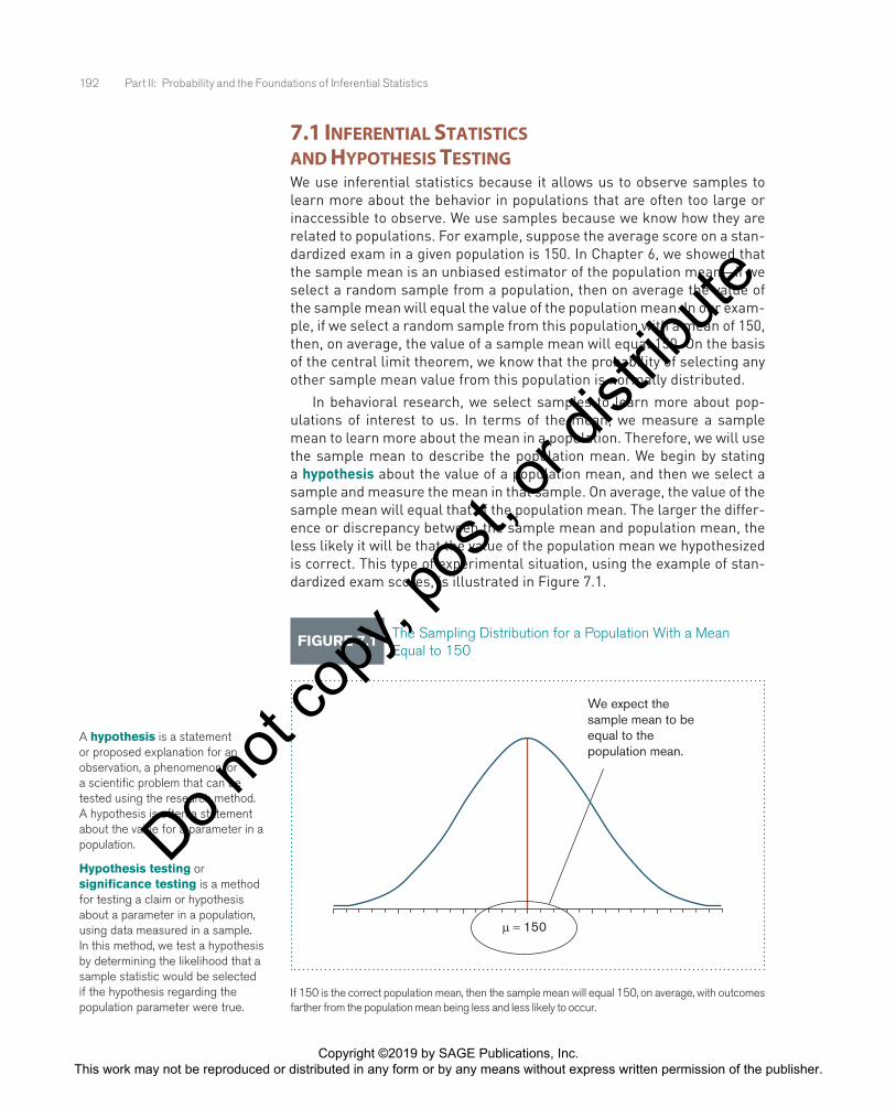
In behavioral research, we select samples to learn more about pop-ulations of interest to us. In terms of the mean, we measure a sample mean to learn more about the mean in a population. Therefore, we will use the sample mean to describe the population mean. We begin by stating a hypothesis about the value of a population mean, and then we select a sample and measure the mean in that sample. On average, the value of the sample mean will equal that of the population mean. The larger the differ-ence or discrepancy between the sample mean and population mean, the less likely it will be that the value of the population mean we hypothesized is correct. This type of experimental situation, using the example of stan-dardized exam scores, is illustrated in Figure 7.1.
FIGURE 7.1 The Sampling Distribution for a Population With a Mean Equal to 150
µ = 150
We expect the sample mean to be equal to the population mean.
If 150 is the correct population mean, then the sample mean will equal 150, on average, with outcomes farther from the population mean being less and less likely to occur.
A hypothesis is a statement or proposed explanation for an observation, a phenomenon, or a scientific problem that can be tested using the research method. A hypothesis is often a statement about the value for a parameter in a population.
Hypothesis testing or significance testing is a method for testing a claim or hypothesis about a parameter in a population, using data measured in a sample. In this method, we test a hypothesis by determining the likelihood that a sample statistic would be selected if the hypothesis regarding the population parameter were true.
Copyright ©2019 by SAGE Publications, Inc. This work may not be reproduced or distributed in any form or by any means without express written permission of the publisher.
Do not
copy
, pos
t, or d
istrib
ute
Chapter 7: Hypothesis Testing 193
The method of evaluating samples to learn more about characteristics in a given population is called hypothesis testing. Hypothesis testing is really a systematic way to test claims or ideas about a group or population. To illus-trate, let us use a simple example concerning social media use. According to estimates reported by Mediakix (2016), the average consumer spends roughly 120 minutes (or 2 hours) a day on social media. Suppose we want to test if pre-millennial-generation consumers use social media comparably to the average consumer. To make a test, we record the time (in minutes) that a sample of pre-millennial consumers use social media per day, and compare this to the average of 120 minutes per day that all consumers (the population) use social media. The mean we measure for these pre-millen-nial consumers is a sample mean. We can then compare the mean in our sample to the population mean for all consumers (µ = 120 minutes).
The method of hypothesis testing can be summarized in four steps. We describe each of these four steps in greater detail in Section 7.2.
1. To begin, we identify a hypothesis or claim that we feel should be tested. For example, we decide to test whether the mean number of minutes per day that pre-millennial consumers spend on social media is 120 minutes per day (i.e., the average for all consumers).
2. We select a criterion upon which we decide whether the hypothesis being tested should be accepted or not. For example, the hypothe-sis is whether or not pre-millennial consumers spend 120 minutes using social media per day. If pre-millennial consumers use social media similar to the average consumer, then we expect the sam-ple mean will be about 120 minutes. If pre-millennial consumers spend more or less than 120 minutes using social media per day, then we expect the sample mean will be some value much lower or higher than 120 minutes. However, at what point do we decide that the discrepancy between the sample mean and 120 minutes (i.e., the population mean) is so big that we can reject the notion that pre-millennial consumers use social media similar to the average consumer? In Step 2 of hypothesis testing, we answer this question.
3. Select a sample from the population and measure the sample mean. For example, we can select a sample of 1,000 pre-millennial consumers and measure the mean time (in minutes) that they use social media per day.
4. Compare what we observe in the sample to what we expect to observe if the claim we are testing—that pre-millennial consum-ers spend 120 minutes using social media per day—is true. We expect the sample mean will be around 120 minutes. The smaller the discrepancy between the sample mean and population mean, the more likely we are to decide that pre-millennial consumers use social media similar to the average consumer (i.e., about 120 min-utes per day). The larger the discrepancy between the sample mean and population mean, the more likely we are to decide to reject that claim.
Hypothesis testing or significance testing is a method for testing a claim or hypothesis about a parameter in a population, using data measured in a sample. In this method, we test a hypothesis by determining the likelihood that a sample statistic would be selected if the hypothesis regarding the population parameter were true.
Copyright ©2019 by SAGE Publications, Inc. This work may not be reproduced or distributed in any form or by any means without express written permission of the publisher.
Do not
copy
, pos
t, or d
istrib
ute
194 Part II: Probability and the Foundations of Inferential Statistics
7.2 four StepS to HypotHeSIS teStIngThe goal of hypothesis testing is to determine the likelihood that a sam-ple statistic would be selected if the hypothesis regarding a population parameter were true. In this section, we describe the four steps of hypoth-esis testing that were briefly introduced in Section 7.1:
Step 1: State the hypotheses.
Step 2: Set the criteria for a decision.
Step 3: Compute the test statistic.
Step 4: Make a decision.
Step 1: State the hypotheses. We begin by stating the value of a population mean in a null hypothesis, which we presume is true. For the example of social media use, we can state the null hypothesis that pre-millennial consumers use an average of 120 minutes of social media per day:
H0: µ = 120.
This is a starting point so that we can decide whether or not the null hypothesis is likely to be true, similar to the presumption of innocence in a courtroom. When a defendant is on trial, the jury starts by assuming that the defendant is innocent. The basis of the decision is to determine whether this assumption is true. Likewise, in hypothesis testing, we start by assuming that the hypothesis or claim we are testing is true. This is stated in the null hypothesis. The basis of the decision is to determine whether this assumption is likely to be true.
The key reason we are testing the null hypothesis is because we think it is wrong. We state what we think is wrong about the null hypothesis in an alternative hypothesis. In a courtroom, the defendant is assumed to be innocent (this is the null hypothesis so to speak), so the burden is on a prosecutor to conduct a trial to show evidence that the defendant is not innocent. In a similar way, we assume the null hypothesis is true, placing the burden on the researcher to conduct a study to show evidence that the null hypothesis is unlikely to be true. Regardless, we always make a decision about the null hypothesis (that it is likely or unlikely to be true). The alternative hypothesis is needed for Step 2.
LEARNING CHECK 1
1. On average, what do we expect the sample mean to be equal to?
2. True or false: Researchers select a sample from a population to learn more about characteristics in that sample.
Answers: 1. The population mean; 2. False. Researchers select a sample from a population to learn more about characteristics in the population from which the sample was selected.
FYIHypothesis testing is a method of testing whether hypotheses about a population parameter are likely to be true.
The null hypothesis (H0), stated as the null, is a statement about a population parameter, such as the population mean, that is assumed to be true, and a hypothesis test is structured to decide whether or not to reject this assumption.
An alternative hypothesis (H1) is a statement that directly contradicts a null hypothesis by stating that the actual value of a population parameter is less than, greater than, or not equal to the value stated in the null hypothesis.
Copyright ©2019 by SAGE Publications, Inc. This work may not be reproduced or distributed in any form or by any means without express written permission of the publisher.
Do not
copy
, pos
t, or d
istrib
ute
Chapter 7: Hypothesis Testing 195
The null and alternative hypotheses must encompass all possibilities for the population mean. For the example of social media use, we can state that the value in the null hypothesis is not equal to (≠) 120 minutes. In this way, the null hypothesis value (µ = 120 minutes) and the alternative hypothesis value (µ ≠ 120) encompass all possible values for the popula-tion mean. If we believe that pre-millennial consumers use more than (>) or less than (<) 120 minutes of social media per day, then we can make a “greater than” or “less than” statement in the alternative hypothesis—this type of alternative is described in Example 7.2 (page 206). Regardless of the decision alternative, the null and alternative hypotheses must encompass all possibilities for the value of the population mean.
FYIIn hypothesis testing, we conduct
a study to test whether the null hypothesis is likely to be true.
MAKING SENSE TESTING THE NULL HYPOTHESIS
A decision made in hypothesis testing relates to the null hypothesis. This means two things in terms of making a decision:
1. Decisions are made about the null hypothesis. Using the courtroom analogy, a jury decides whether a defendant is guilty or not guilty. The jury does not make a decision of guilty or innocent because the defendant is assumed to be innocent. All evidence presented in a trial is to show that a defendant is guilty. The evidence either shows guilt (decision: guilty) or does not (decision: not guilty). In a similar way, the null hypothesis is assumed to be correct. A researcher conducts a study showing evidence that this assumption is unlikely (we reject the null hypothesis) or fails to do so (we retain the null hypothesis).
2. The bias is to do nothing. Using the courtroom analogy, for the same reason the courts would rather let the guilty go free than send the innocent to prison, researchers would rather do nothing (accept previous notions of truth stated by a null hypothesis) than make statements that are not correct. For this reason, we assume the null hypothesis is correct, thereby placing the burden on the researcher to demonstrate that the null hypothesis is not likely to be correct. Keep in mind, however, that when we retain the null hypothesis, this does not mean that the null hypothesis is correct. Instead, it means that there is insufficient evidence to reject it; it is not possible to prove the null hypothesis.
Step 2: Set the criteria for a decision. To set the criteria for a decision, we state the level of significance for a hypothesis test. This is similar to the crite-rion that jurors use in a criminal trial. Jurors decide whether the evidence presented shows guilt beyond a reasonable doubt (this is the criterion). Likewise, in hypothesis testing, we collect data to test whether or not the null hypothesis is retained, based on the likelihood of selecting a sample mean from a population (the likelihood is the criterion). The likelihood or level of significance is typically set at 5% in behavioral research studies. When the probability of obtaining a sample mean would be less than 5% if the null hypothesis were true, then we conclude that the sample we selected is too unlikely, and thus we reject the null hypothesis.
The alternative hypothesis is identified so that the criterion can be spe-cifically stated. Remember that the sample mean will equal the population mean on average if the null hypothesis is true. All other possible values of the sample mean are normally distributed (central limit theorem). The empirical rule tells us that at least 95% of all sample means fall within
Level of significance, or significance level, is a criterion of judgment upon which a decision is made regarding the value stated in a null hypothesis. The criterion is based on the probability of obtaining a statistic measured in a sample if the value stated in the null hypothesis were true.
Copyright ©2019 by SAGE Publications, Inc. This work may not be reproduced or distributed in any form or by any means without express written permission of the publisher.
Do not
copy
, pos
t, or d
istrib
ute
196 Part II: Probability and the Foundations of Inferential Statistics
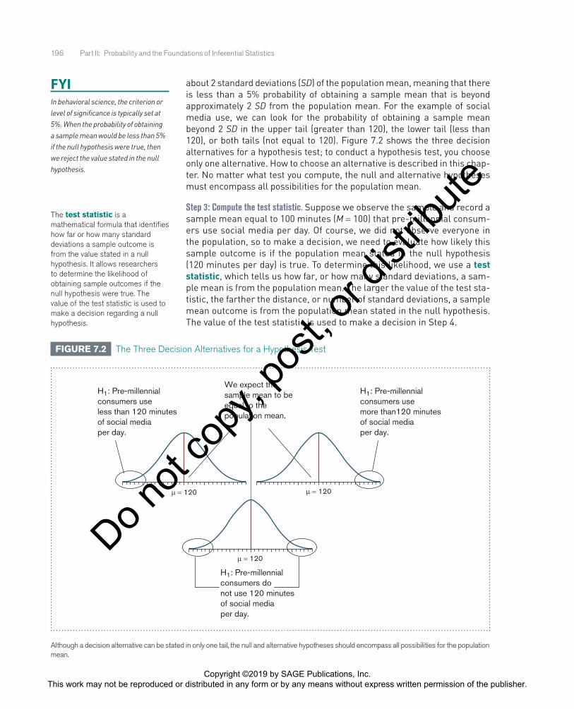
about 2 standard deviations (SD) of the population mean, meaning that there is less than a 5% probability of obtaining a sample mean that is beyond approximately 2 SD from the population mean. For the example of social media use, we can look for the probability of obtaining a sample mean beyond 2 SD in the upper tail (greater than 120), the lower tail (less than 120), or both tails (not equal to 120). Figure 7.2 shows the three decision alternatives for a hypothesis test; to conduct a hypothesis test, you choose only one alternative. How to choose an alternative is described in this chap-ter. No matter what test you compute, the null and alternative hypotheses must encompass all possibilities for the population mean.
Step 3: Compute the test statistic. Suppose we observe the sample and record a sample mean equal to 100 minutes (M = 100) that pre-millennial consum-ers use social media per day. Of course, we did not observe everyone in the population, so to make a decision, we need to evaluate how likely this sample outcome is if the population mean stated in the null hypothesis (120 minutes per day) is true. To determine this likelihood, we use a test statistic, which tells us how far, or how many standard deviations, a sam-ple mean is from the population mean. The larger the value of the test sta-tistic, the farther the distance, or number of standard deviations, a sample mean outcome is from the population mean stated in the null hypothesis. The value of the test statistic is used to make a decision in Step 4.
FYIIn behavioral science, the criterion or level of significance is typically set at 5%. When the probability of obtaining a sample mean would be less than 5% if the null hypothesis were true, then we reject the value stated in the null hypothesis.
The test statistic is a mathematical formula that identifies how far or how many standard deviations a sample outcome is from the value stated in a null hypothesis. It allows researchers to determine the likelihood of obtaining sample outcomes if the null hypothesis were true. The value of the test statistic is used to make a decision regarding a null hypothesis.
FIGURE 7.2 The Three Decision Alternatives for a Hypothesis Test
µ = 120
We expect the sample mean to be equal to the population mean.
µ = 120
µ = 120
H1: Pre-millennialconsumers usemore than120 minutes of social media per day.
H1: Pre-millennialconsumers useless than 120 minutes of social media per day.
H1: Pre-millennialconsumers donot use 120 minutes of social media per day.
Although a decision alternative can be stated in only one tail, the null and alternative hypotheses should encompass all possibilities for the population mean.
Copyright ©2019 by SAGE Publications, Inc. This work may not be reproduced or distributed in any form or by any means without express written permission of the publisher.
Do not
copy
, pos
t, or d
istrib
ute
Chapter 7: Hypothesis Testing 197
Step 4: Make a decision. We use the value of the test statistic to make a deci-sion about the null hypothesis. The decision is based on the probability of obtaining a sample mean, given that the value stated in the null hypothesis is true. If the probability of obtaining a sample mean is less than or equal to 5% when the null hypothesis is true, then the decision is to reject the null hypothesis. If the probability of obtaining a sample mean is greater than 5% when the null hypothesis is true, then the decision is to retain the null hypothesis. In sum, there are two decisions a researcher can make:
1. Reject the null hypothesis. The sample mean is associated with a low probability of occurrence when the null hypothesis is true. For this decision, we conclude that the value stated in the null hypoth-esis is wrong; it is rejected.
2. Retain the null hypothesis. The sample mean is associated with a high probability of occurrence when the null hypothesis is true. For this decision, we conclude that there is insufficient evidence to reject the null hypothesis; this does not mean that the null hypoth-esis is correct. It is not possible to prove the null hypothesis.
The probability of obtaining a sample mean, given that the value stated in the null hypothesis is true, is stated by the p value. The p value is a probability: It varies between 0 and 1 and can never be negative. In Step 2, we stated the criterion or probability of obtaining a sample mean at which point we will decide to reject the value stated in the null hypothesis, which is typically set at 5% in behavioral research. To make a decision, we com-pare the p value to the criterion we set in Step 2.
When the p value is less than 5% (p < .05), we reject the null hypothesis, and when p = .05, the decision is also to reject the null hypothesis. When the p value is greater than 5% (p > .05), we retain the null hypothesis. The decision to reject or retain the null hypothesis is called significance. When the p value is less than or equal to .05, we reach significance; the decision is to reject the null hypothesis. When the p value is greater than .05, we fail to reach significance; the decision is to retain the null hypothesis. Figure 7.3 summarizes the four steps of hypothesis testing.
FYIWe use the value of the test statistic
to make a decision regarding the null hypothesis.
FYIResearchers make decisions
regarding the null hypothesis. The decision can be to retain the null
(p > .05) or reject the null (p ≤ .05).
A p value is the probability of obtaining a sample outcome, given that the value stated in the null hypothesis is true. The p value for obtaining a sample outcome is compared to the level of significance or criterion for making a decision.
Significance, or statistical significance, describes a decision made concerning a value stated in the null hypothesis. When the null hypothesis is rejected, we reach significance. When the null hypothesis is retained, we fail to reach significance.
LEARNING CHECK 2
1. State the four steps of hypothesis testing.
2. The decision in hypothesis testing is to retain or reject which hypothesis: null or alternative?
3. The criterion or level of significance in behavioral research is typically set at what probability value?
4. A test statistic is associated with a p value less than .05. What is the decision for this hypothesis test?
5. If the null hypothesis is rejected, did we reach significance?
Answers: 1. Step 1: State the hypotheses. Step 2: Set the criteria for a decision. Step 3: Compute the test statistic. Step 4: Make a decision; 2. Null hypothesis; 3. The level of significance is typically set at .05; 4. Reject the null hypothesis; 5. Yes.
Copyright ©2019 by SAGE Publications, Inc. This work may not be reproduced or distributed in any form or by any means without express written permission of the publisher.
Do not
copy
, pos
t, or d
istrib
ute
198 Part II: Probability and the Foundations of Inferential Statistics
7.3 HypotHeSIS teStIng and SamplIng dIStrIbutIonSThe application of hypothesis testing is rooted in an understanding of the sampling distribution of the mean. In Chapter 6, we showed three characteristics of the mean, two of which are particularly relevant in this section:
1. The sample mean is an unbiased estimator of the population mean. On average, a randomly selected sample will have a mean equal to that in the population. In hypothesis testing, we begin by stating the null hypothesis. We expect that, if the null hypothe-sis is true, then a random sample selected from a given popula-tion will have a sample mean equal to the value stated in the null hypothesis.
2. Regardless of the distribution in a given population, the sampling distribution of the sample mean is approximately normal. Hence,
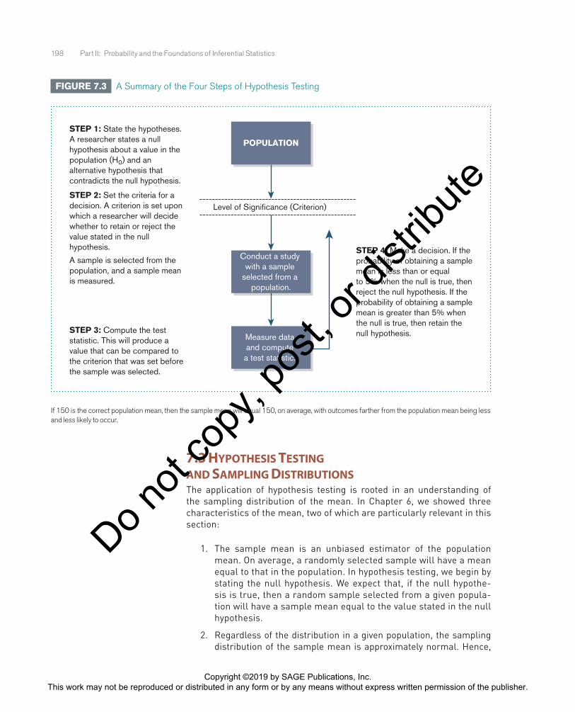
FIGURE 7.3 A Summary of the Four Steps of Hypothesis Testing
-------------------------------------------------- Level of Significance (Criterion)
--------------------------------------------------
POPULATION
STEP 1: State the hypotheses. A researcher states a null hypothesis about a value in the population (H0) and an alternative hypothesis that contradicts the null hypothesis.
Conduct a study with a sample
selected from a population.
STEP 2: Set the criteria for a decision. A criterion is set uponwhich a researcher will decide whether to retain or reject the value stated in the null hypothesis.
A sample is selected from thepopulation, and a sample mean is measured.
Measure data and compute a test statistic.
STEP 3: Compute the test statistic. This will produce a value that can be compared to the criterion that was set before the sample was selected.
STEP 4: Make a decision. If theprobability of obtaining a samplemean is less than or equalto 5% when the null is true, thenreject the null hypothesis. If theprobability of obtaining a samplemean is greater than 5% whenthe null is true, then retain thenull hypothesis.
If 150 is the correct population mean, then the sample mean will equal 150, on average, with outcomes farther from the population mean being less and less likely to occur.
Copyright ©2019 by SAGE Publications, Inc. This work may not be reproduced or distributed in any form or by any means without express written permission of the publisher.
Do not
copy
, pos
t, or d
istrib
ute
Chapter 7: Hypothesis Testing 199
the probabilities of all other possible sample means we could select are normally distributed. Using this distribution, we can therefore state an alternative hypothesis to locate the probability of obtaining sample means with less than a 5% chance of being selected if the value stated in the null hypothesis is true. Figure 7.2 shows that we can identify sample mean outcomes in one or both tails using the normal distribution.
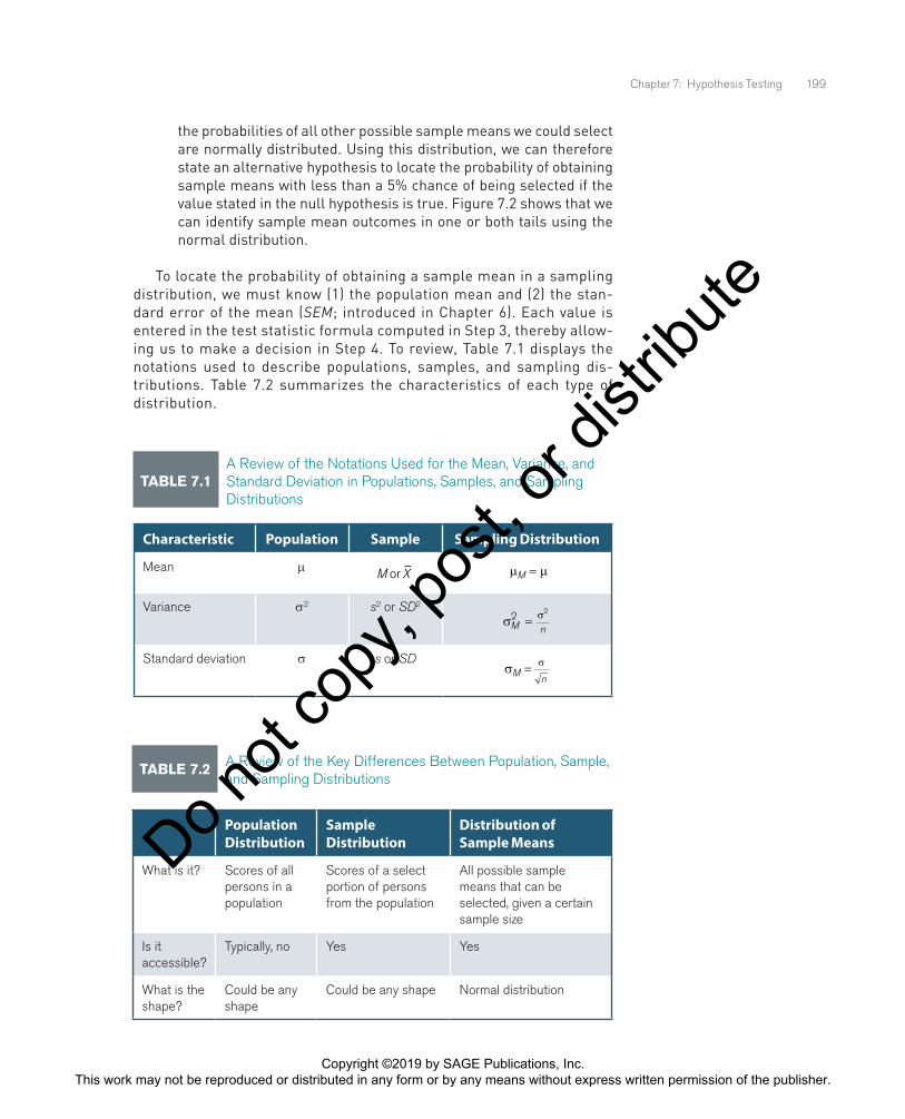
To locate the probability of obtaining a sample mean in a sampling distribution, we must know (1) the population mean and (2) the stan-dard error of the mean (SEM; introduced in Chapter 6). Each value is entered in the test statistic formula computed in Step 3, thereby allow-ing us to make a decision in Step 4. To review, Table 7.1 displays the notations used to describe populations, samples, and sampling dis-tributions. Table 7.2 summarizes the characteristics of each type of distribution.
TABLE 7.1 A Review of the Notations Used for the Mean, Variance, and Standard Deviation in Populations, Samples, and Sampling Distributions
Characteristic Population Sample Sampling Distribution
Mean µ M Xor µ µM =
Variance σ2 s2 or SD2
σ σM n2 2
=
Standard deviation σ s or SDσ σ
Mn
=
TABLE 7.2 A Review of the Key Differences Between Population, Sample, and Sampling Distributions
Population Distribution
Sample Distribution
Distribution of Sample Means
What is it? Scores of all persons in a population
Scores of a select portion of persons from the population
All possible sample means that can be selected, given a certain sample size
Is it accessible?
Typically, no Yes Yes
What is the shape?
Could be any shape
Could be any shape Normal distribution
Copyright ©2019 by SAGE Publications, Inc. This work may not be reproduced or distributed in any form or by any means without express written permission of the publisher.
Do not
copy
, pos
t, or d
istrib
ute
200 Part II: Probability and the Foundations of Inferential Statistics
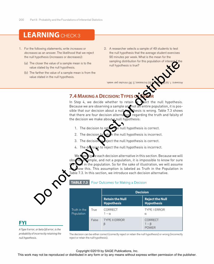
7.4 makIng a decISIon: typeS of errorIn Step 4, we decide whether to retain or reject the null hypothesis. Because we are observing a sample and not an entire population, it is pos-sible that our decision about a null hypothesis is wrong. Table 7.3 shows that there are four decision alternatives regarding the truth and falsity of the decision we make about a null hypothesis:
1. The decision to retain the null hypothesis is correct.
2. The decision to retain the null hypothesis is incorrect.
3. The decision to reject the null hypothesis is correct.
4. The decision to reject the null hypothesis is incorrect.
We investigate each decision alternative in this section. Because we will observe a sample, and not a population, it is impossible to know for sure the truth in the population. So for the sake of illustration, we will assume we know this. This assumption is labeled as Truth in the Population in Table 7.3. In this section, we introduce each decision alternative.
LEARNING CHECK 3
1. For the following statements, write increases or decreases as an answer. The likelihood that we reject the null hypothesis (increases or decreases):
(a) The closer the value of a sample mean is to the value stated by the null hypothesis.
(b) The farther the value of a sample mean is from the value stated in the null hypothesis.
2. A researcher selects a sample of 49 students to test the null hypothesis that the average student exercises 90 minutes per week. What is the mean for the sampling distribution for this population of interest if the null hypothesis is true?
Answers: 1. (a) Decreases, (b) Increases; 2. 90 minutes per week. TABLE 7.3 Four Outcomes for Making a Decision
Decision
Retain the Null Hypothesis
Reject the Null Hypothesis
Truth in the Population
True CORRECT1 − α
TYPE I ERRORα
False TYPE II ERRORβ
CORRECT1 − βPOWER
The decision can be either correct (correctly reject or retain the null hypothesis) or wrong (incorrectly reject or retain the null hypothesis).
FYIA Type II error, or beta (β) error, is the probability of incorrectly retaining the null hypothesis.
Copyright ©2019 by SAGE Publications, Inc. This work may not be reproduced or distributed in any form or by any means without express written permission of the publisher.
Do not
copy
, pos
t, or d
istrib
ute
Chapter 7: Hypothesis Testing 201
Decision: Retain the Null HypothesisWhen we decide to retain the null hypothesis, we can be correct or incor-rect. The correct decision is to retain a true null hypothesis. This deci-sion is called a null result or null finding. This is usually an uninteresting decision because the decision is to retain what we already assumed. For this reason, a null result alone is rarely published in scientific journals for behavioral research.
The incorrect decision is to retain a false null hypothesis: a “false negative” finding. This decision is an example of a Type II error, or beta (β) error. With each test we make, there is always some probabil-ity that the decision is a Type II error. In this decision, we decide not to reject previous notions of truth that are in fact false. While this type of error is often regarded as less problematic than a Type I error (defined in the next paragraph), it can be problematic in many fields, such as in medicine where testing of treatments could mean life or death for patients.
Decision: Reject the Null HypothesisWhen we decide to reject the null hypothesis, we can be correct or incor-rect. The incorrect decision is to reject a true null hypothesis: a “false positive” finding. This decision is an example of a Type I error. With each test we make, there is always some probability that our decision is a Type I error. A researcher who makes this error decides to reject previous notions of truth that are in fact true. Using the courtroom analogy, making this type of error is analogous to finding an innocent person guilty. To minimize this error, we therefore place the burden on the researcher to demonstrate evidence that the null hypothesis is indeed false.
Because we assume the null hypothesis is true, we control for Type I error by stating a level of significance. The level we set, called the alpha level (symbolized as α), is the largest probability of commit-ting a Type I error that we will allow and still decide to reject the null hypothesis. This criterion is usually set at .05 (α = .05) in behavioral research. To make a decision, we compare the alpha level (or criterion) to the p value (the actual likelihood of obtaining a sample mean, if the null were true). When the p value is less than the criterion of α = .05, we decide to reject the null hypothesis; otherwise, we retain the null hypothesis.
The correct decision is to reject a false null hypothesis. In other words, we decide that the null hypothesis is false when it is indeed false. This decision is called the power of the decision-making process because it is the decision we aim for. Remember that we are only test-ing the null hypothesis because we think it is wrong. Deciding to reject a false null hypothesis, then, is the power, inasmuch as we learn the most about populations when we accurately reject false notions of truth about them. This decision is the most published result in behavioral research.
FYIResearchers directly control for the
probability of a Type I error by stating an alpha (α) level.
FYIThe power in hypothesis testing is
the probability of correctly rejecting a value stated in the null hypothesis.
Type II error, or beta (β) error, is the probability of retaining a null hypothesis that is actually false.
Type I error is the probability of rejecting a null hypothesis that is actually true. Researchers directly control for the probability of committing this type of error by stating an alpha level.
An alpha (α) level is the level of significance or criterion for a hypothesis test. It is the largest probability of committing a Type I error that we will allow and still decide to reject the null hypothesis.
The power in hypothesis testing is the probability of rejecting a false null hypothesis. Specifically, it is the probability that a randomly selected sample will show that the null hypothesis is false when the null hypothesis is indeed false.
Copyright ©2019 by SAGE Publications, Inc. This work may not be reproduced or distributed in any form or by any means without express written permission of the publisher.
Do not
copy
, pos
t, or d
istrib
ute
202 Part II: Probability and the Foundations of Inferential Statistics
7.5 teStIng for SIgnIfIcance: exampleS uSIng tHe z teStWe use hypothesis testing to make decisions about parameters in a pop-ulation. The type of test statistic we use in hypothesis testing depends largely on what is known in a population. When we know the mean and standard deviation in a single population, we can use the one-sample z test, which we use in this section to illustrate the four steps of hypothe-sis testing.
Recall that we can state one of three alternative hypotheses: A popu-lation mean is greater than (>), less than (<), or not equal to (≠) the value stated in a null hypothesis. The alternative hypothesis determines which tail of a sampling distribution to place the level of significance in, as illus-trated in Figure 7.2. In this section, we will use an example for a directional and a nondirectional hypothesis test.
Nondirectional Tests (H1: ≠)In Example 7.1, we use the one-sample z test for a nondirectional, or two-tailed, test, where the alternative hypothesis is stated as not equal to (≠) the null hypothesis. For this test, we will place the level of significance in both tails of the sampling distribution. We are therefore interested in any alternative to the null hypothesis. This is the most common alternative hypothesis tested in behavioral science.
Example 7.1
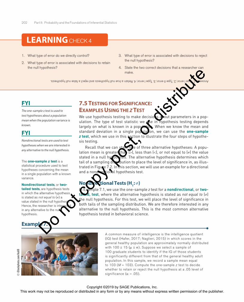
A common measure of intelligence is the intelligence quotient (IQ) test (Hafer, 2017; Naglieri, 2015) in which scores in the general healthy population are approximately normally distributed with 100 ± 15 (µ ± σ) . Suppose we select a sample of 100 graduate students to identify if the IQ of those students is significantly different from that of the general healthy adult population. In this sample, we record a sample mean equal to 103 (M = 103) . Compute the one-sample z test to decide whether to retain or reject the null hypothesis at a .05 level of significance (α = .05) .
LEARNING CHECK 4
1. What type of error do we directly control?
2. What type of error is associated with decisions to retain the null hypothesis?
3. What type of error is associated with decisions to reject the null hypothesis?
4. State the two correct decisions that a researcher can make.
Answers: 1. Type I error; 2. Type II error; 3. Type I error; 4. Retain a true null hypothesis and reject a false null hypothesis.
The one-sample z test is a statistical procedure used to test hypotheses concerning the mean in a single population with a known variance.
Nondirectional tests, or two-tailed tests, are hypothesis tests in which the alternative hypothesis is stated as not equal to (≠) a value stated in the null hypothesis. Hence, the researcher is interested in any alternative to the null hypothesis.
FYIThe one-sample z test is used to test hypotheses about a population mean when the population variance is known.
FYINondirectional tests are used to test hypotheses when we are interested in any alternative to the null hypothesis.
iS
tock
phot
o.com
/kali
9
Copyright ©2019 by SAGE Publications, Inc. This work may not be reproduced or distributed in any form or by any means without express written permission of the publisher.
Do not
copy
, pos
t, or d
istrib
ute
Chapter 7: Hypothesis Testing 203
Step 1: State the hypotheses. The population mean IQ score is 100; therefore, µ = 100 is the null hypothesis. We are testing whether the null hypothesis is (=) or is not (≠) likely to be true among graduate students:
H0: µ = 100 Mean IQ scores are equal to 100 in the population of graduate students.
H1: µ ≠ 100 Mean IQ scores are not equal to 100 in the population of graduate students.
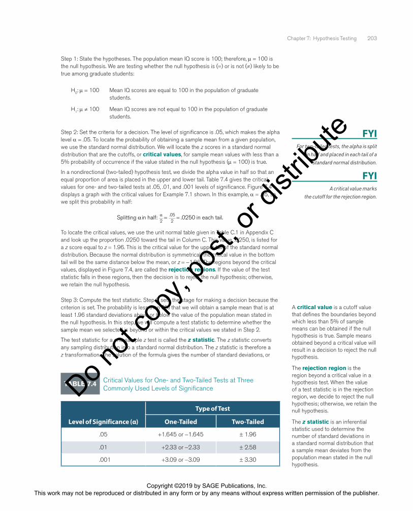
Step 2: Set the criteria for a decision. The level of significance is .05, which makes the alpha level α = .05. To locate the probability of obtaining a sample mean from a given population, we use the standard normal distribution. We will locate the z scores in a standard normal distribution that are the cutoffs, or critical values, for sample mean values with less than a 5% probability of occurrence if the value stated in the null hypothesis (µ = 100) is true.
In a nondirectional (two-tailed) hypothesis test, we divide the alpha value in half so that an equal proportion of area is placed in the upper and lower tail. Table 7.4 gives the critical values for one- and two-tailed tests at .05, .01, and .001 levels of significance. Figure 7.4 displays a graph with the critical values for Example 7.1 shown. In this example, α = .05, so we split this probability in half:
Splitting in half: in each tail.α α2
052
0250= =. .
To locate the critical values, we use the unit normal table given in Table C.1 in Appendix C and look up the proportion .0250 toward the tail in Column C. This value, .0250, is listed for a z score equal to z = 1.96. This is the critical value for the upper tail of the standard normal distribution. Because the normal distribution is symmetrical, the critical value in the bottom tail will be the same distance below the mean, or z = −1.96. The regions beyond the critical values, displayed in Figure 7.4, are called the rejection regions. If the value of the test statistic falls in these regions, then the decision is to reject the null hypothesis; otherwise, we retain the null hypothesis.
Step 3: Compute the test statistic. Step 2 sets the stage for making a decision because the criterion is set. The probability is less than 5% that we will obtain a sample mean that is at least 1.96 standard deviations above or below the value of the population mean stated in the null hypothesis. In this step, we will compute a test statistic to determine whether the sample mean we selected is beyond or within the critical values we stated in Step 2.
The test statistic for a one-sample z test is called the z statistic. The z statistic converts any sampling distribution into a standard normal distribution. The z statistic is therefore a z transformation. The solution of the formula gives the number of standard deviations, or
A critical value is a cutoff value that defines the boundaries beyond which less than 5% of sample means can be obtained if the null hypothesis is true. Sample means obtained beyond a critical value will result in a decision to reject the null hypothesis.
The rejection region is the region beyond a critical value in a hypothesis test. When the value of a test statistic is in the rejection region, we decide to reject the null hypothesis; otherwise, we retain the null hypothesis.
The z statistic is an inferential statistic used to determine the number of standard deviations in a standard normal distribution that a sample mean deviates from the population mean stated in the null hypothesis.
TABLE 7.4 Critical Values for One- and Two-Tailed Tests at Three Commonly Used Levels of Significance
Type of Test
Level of Significance (α) One-Tailed Two-Tailed
.05 +1.645 or −1.645 ± 1.96
.01 +2.33 or −2.33 ± 2.58
.001 +3.09 or −3.09 ± 3.30
FYIFor two-tailed tests, the alpha is split
in half and placed in each tail of a standard normal distribution.
FYIA critical value marks
the cutoff for the rejection region.
Copyright ©2019 by SAGE Publications, Inc. This work may not be reproduced or distributed in any form or by any means without express written permission of the publisher.
Do not
copy
, pos
t, or d
istrib
ute

204 Part II: Probability and the Foundations of Inferential Statistics
z scores, that a sample mean falls above or below the population mean stated in the null hypothesis. We can then compare the value of the z statistic, called the obtained value, to the critical values we determined in Step 2. The z statistic formula is the sample mean minus the population mean stated in the null hypothesis, divided by the standard error of the mean:
z statistic: obtz MM
M n= =−µ
σσσ, .where
To calculate the z statistic, first compute the standard error (σM), which is the denominator for the z statistic:
σMn
= ==σ 15
1001 50. .
Then compute the z statistic by substituting the values of the sample mean, M = 103; the population mean stated by the null hypothesis, µ = 100; and the standard error we just calculated, σM = 1.50:
zM
Mobt = =
−=
−µ
σ
1032.00
100
1 50..
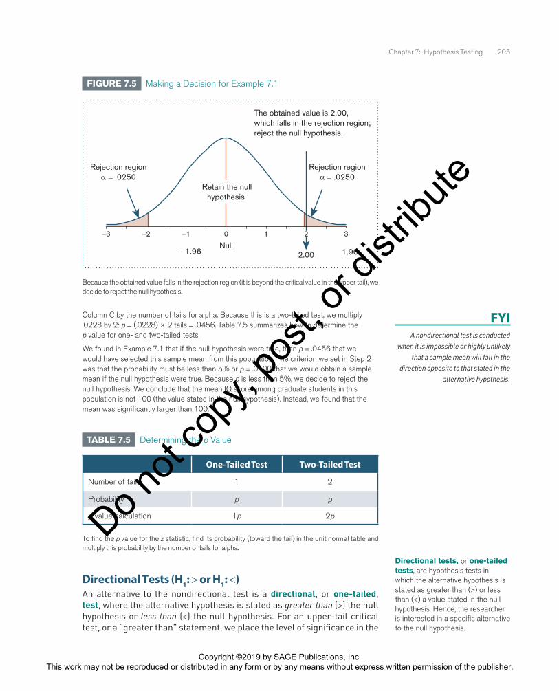
Step 4: Make a decision. To make a decision, we compare the obtained value to the critical values. We reject the null hypothesis if the obtained value exceeds a critical value. Figure 7.5 shows that the obtained value (zobt = 2.00) is greater than the critical value; it falls in the rejection region. The decision for this test is to reject the null hypothesis.
The probability of obtaining zobt = 2.00 is stated by the p value. To locate the p value or probability of obtaining the z statistic, we refer to the unit normal table in Table C.1 in Appendix C. Look for a z score equal to 2.00 in Column A, then locate the probability toward the tail in Column C. The value is .0228. Finally, multiply the value given in
FIGURE 7.4 The Critical Values (± 1.96) for a Nondirectional (two-tailed) Test With a .05 Level of Significance
Critical values for a nondirectional (two-tailed) test with α = .05
−1.96 1.96
Rejection region α = .0250
Rejection region α = .0250
0−1−2−3Null
21 3
The obtained value is the value of a test statistic. This value is compared to the critical value(s) of a hypothesis test to make a decision. When the obtained value exceeds a critical value, we decide to reject the null hypothesis; otherwise, we retain the null hypothesis.
FYIThe z statistic measures the number of standard deviations, or z scores, that a sample mean falls above or below the population mean stated in the null hypothesis.
Copyright ©2019 by SAGE Publications, Inc. This work may not be reproduced or distributed in any form or by any means without express written permission of the publisher.
Do not
copy
, pos
t, or d
istrib
ute
Chapter 7: Hypothesis Testing 205
Column C by the number of tails for alpha. Because this is a two-tailed test, we multiply .0228 by 2: p = (.0228) × 2 tails = .0456. Table 7.5 summarizes how to determine the p value for one- and two-tailed tests.
We found in Example 7.1 that if the null hypothesis were true, then p = .0456 that we would have selected this sample mean from this population. The criterion we set in Step 2 was that the probability must be less than 5% or p = .0500 that we would obtain a sample mean if the null hypothesis were true. Because p is less than 5%, we decide to reject the null hypothesis. We conclude that the mean IQ score among graduate students in this population is not 100 (the value stated in the null hypothesis). Instead, we found that the mean was significantly larger than 100.
FIGURE 7.5 Making a Decision for Example 7.1
The obtained value is 2.00,which falls in the rejection region;reject the null hypothesis.
Rejection region α = .0250
Rejection region α = .0250
0−1 1 3−2−3
2.00Null
Retain the nullhypothesis
2
−1.96 1.96
Because the obtained value falls in the rejection region (it is beyond the critical value in the upper tail), we decide to reject the null hypothesis.
FYIA nondirectional test is conducted
when it is impossible or highly unlikely that a sample mean will fall in the
direction opposite to that stated in the alternative hypothesis.
TABLE 7.5 Determining the p Value
One-Tailed Test Two-Tailed Test
Number of tails 1 2
Probability p p
p value calculation 1p 2p
To find the p value for the z statistic, find its probability (toward the tail) in the unit normal table and multiply this probability by the number of tails for alpha.
Directional Tests (H1: > or H1: <)An alternative to the nondirectional test is a directional, or one-tailed, test, where the alternative hypothesis is stated as greater than (>) the null hypothesis or less than (<) the null hypothesis. For an upper-tail critical test, or a “greater than” statement, we place the level of significance in the
Directional tests, or one-tailed tests, are hypothesis tests in which the alternative hypothesis is stated as greater than (>) or less than (<) a value stated in the null hypothesis. Hence, the researcher is interested in a specific alternative to the null hypothesis.
Copyright ©2019 by SAGE Publications, Inc. This work may not be reproduced or distributed in any form or by any means without express written permission of the publisher.
Do not
copy
, pos
t, or d
istrib
ute

206 Part II: Probability and the Foundations of Inferential Statistics
upper tail of the sampling distribution. So we are interested in any alter-native greater than the value stated in the null hypothesis. This test can be used when it is impossible or highly unlikely that a sample mean will fall below the population mean stated in the null hypothesis.
For a lower-tail critical test, or a “less than” statement, we place the level of significance or critical value in the lower tail of the sampling dis-tribution. So we are interested in any alternative less than the value stated in the null hypothesis. This test can be used when it is impossible or highly unlikely that a sample mean will fall above the population mean stated in the null hypothesis.
To illustrate how to make a decision using the one-tailed test, we work in Example 7.2 with an example in which such a test could be used.
Example 7.2
Researchers in areas of child development and education are often interested in evaluating methods to promote reading proficiency and academic success (Crosnoe, Benner, & Davis-Kean, 2016; Phillips, Norris, Hayward, & Lovell, 2017). Suppose, for example, researchers were interested in looking at improvement in reading proficiency among elementary school students following a reading program. In this example, the reading program should, if anything, improve reading skills, so if any outcome were possible, it should be to see improvement. For this reason, we could use a one-tailed test to evaluate these data. Suppose elementary school children in the general population show reading proficiency increases of 12 ± 4 (µ ± σ) points on a given standardized measure. If we select a sample of 25 elementary school children in the reading program and record a sample mean improvement in reading proficiency equal to 14
(M = 14) points, then we compute the one-sample z test at a .05 level of significance to determine if the reading program was effective.
Step 1: State the hypotheses. The population mean is 12, and we are testing whether the alternative is greater than (>) this value:
H0: µ ≤ 12 With the reading program, mean improvement is at most 12 points in the population.
H1: µ > 12 With the reading program, mean improvement is greater than 12 points in the population.
Notice a key change for one-tailed tests: The null hypothesis encompasses outcomes in all directions that are opposite the alternative hypothesis. In other words, the directional statement is incorporated into the statement of both hypotheses. In this example, the reading program is intended to improve reading proficiency. Therefore, a one-tailed test is used because there is a specific, expected, logical direction for the effect if the reading program were effective. The null hypothesis therefore states that the expected effect will not occur (that mean improvement will be at most 12 points), and the alternative hypothesis states that the expected effect will occur (that mean improvement will be greater than 12 points).
Step 2: Set the criteria for a decision. The level of significance is .05, which makes the alpha level α = .05. To determine the critical value for an upper-tail critical test, we locate the probability .0500 toward the tail in Column C in the unit normal table in Table C.1 in
iS
tock
phot
o.com
/ Mar
i
Copyright ©2019 by SAGE Publications, Inc. This work may not be reproduced or distributed in any form or by any means without express written permission of the publisher.
Do not
copy
, pos
t, or d
istrib
ute
Chapter 7: Hypothesis Testing 207
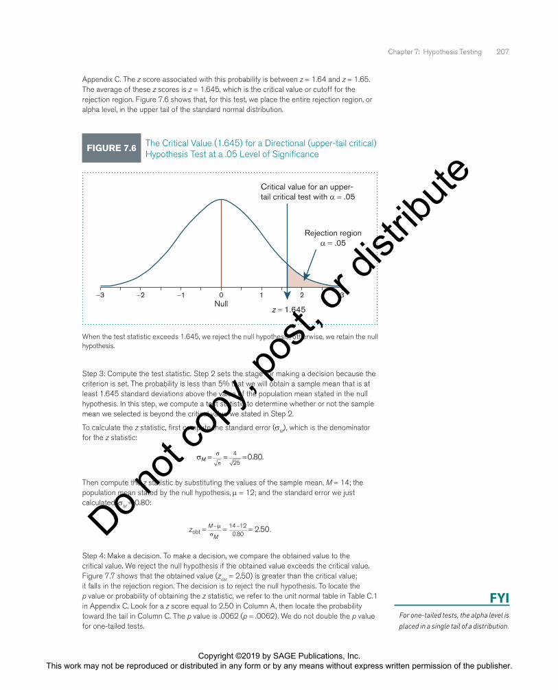
Appendix C. The z score associated with this probability is between z = 1.64 and z = 1.65. The average of these z scores is z = 1.645, which is the critical value or cutoff for the rejection region. Figure 7.6 shows that, for this test, we place the entire rejection region, or alpha level, in the upper tail of the standard normal distribution.
FIGURE 7.6 The Critical Value (1.645) for a Directional (upper-tail critical) Hypothesis Test at a .05 Level of Significance
z = 1.645
Critical value for an upper-tail critical test with α = .05
Rejection region α = .05
0−1−2−3Null
21 3
When the test statistic exceeds 1.645, we reject the null hypothesis; otherwise, we retain the null hypothesis.
Step 3: Compute the test statistic. Step 2 sets the stage for making a decision because the criterion is set. The probability is less than 5% that we will obtain a sample mean that is at least 1.645 standard deviations above the value of the population mean stated in the null hypothesis. In this step, we compute a test statistic to determine whether or not the sample mean we selected is beyond the critical value we stated in Step 2.
To calculate the z statistic, first compute the standard error (σM), which is the denominator for the z statistic:
σMn
= = =σ 4
250 80. .
Then compute the z statistic by substituting the values of the sample mean, M = 14; the population mean stated by the null hypothesis, µ = 12; and the standard error we just calculated, σM = 0.80:
z M
Mobt 2.50= = =− −µ
σ14 12
0 80..
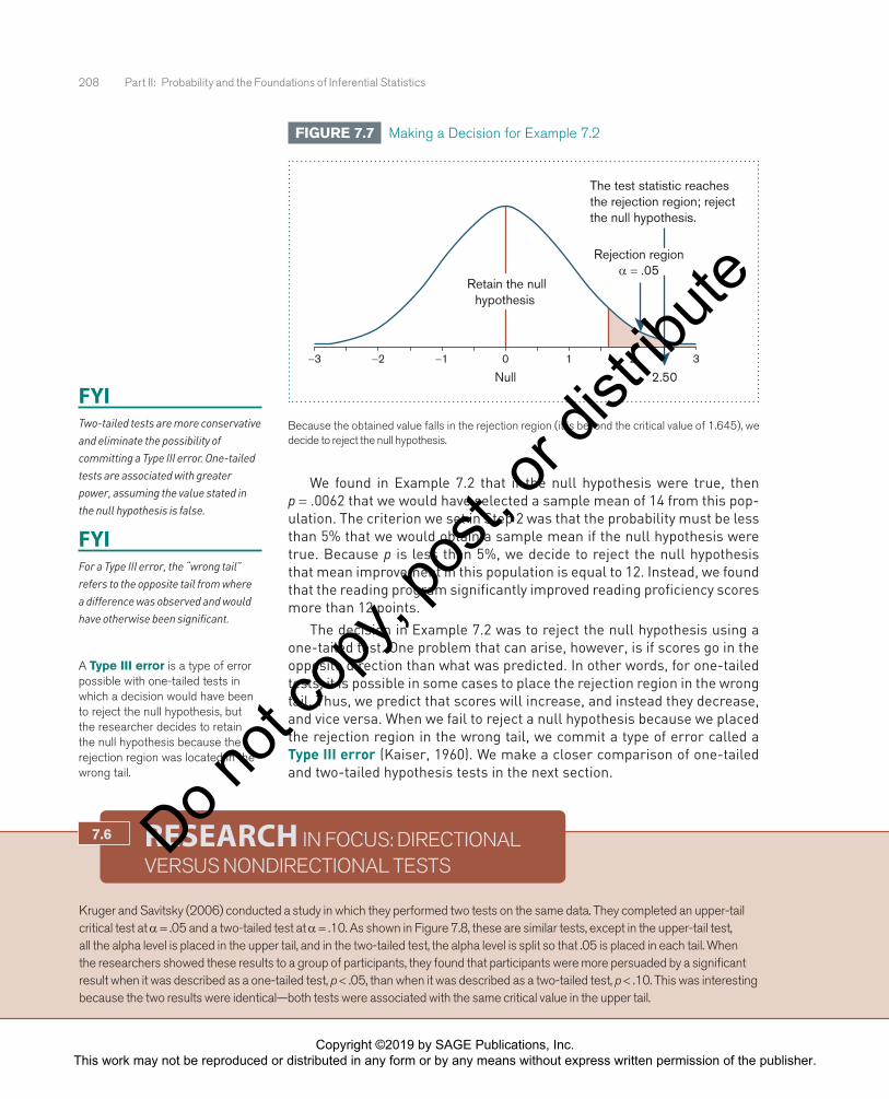
Step 4: Make a decision. To make a decision, we compare the obtained value to the critical value. We reject the null hypothesis if the obtained value exceeds the critical value. Figure 7.7 shows that the obtained value (zobt = 2.50) is greater than the critical value; it falls in the rejection region. The decision is to reject the null hypothesis. To locate the p value or probability of obtaining the z statistic, we refer to the unit normal table in Table C.1 in Appendix C. Look for a z score equal to 2.50 in Column A, then locate the probability toward the tail in Column C. The p value is .0062 (p = .0062). We do not double the p value for one-tailed tests.
FYIFor one-tailed tests, the alpha level is placed in a single tail of a distribution.
Copyright ©2019 by SAGE Publications, Inc. This work may not be reproduced or distributed in any form or by any means without express written permission of the publisher.
Do not
copy
, pos
t, or d
istrib
ute
208 Part II: Probability and the Foundations of Inferential Statistics
We found in Example 7.2 that if the null hypothesis were true, then p = .0062 that we would have selected a sample mean of 14 from this pop-ulation. The criterion we set in Step 2 was that the probability must be less than 5% that we would obtain a sample mean if the null hypothesis were true. Because p is less than 5%, we decide to reject the null hypothesis that mean improvement in this population is equal to 12. Instead, we found that the reading program significantly improved reading proficiency scores more than 12 points.
The decision in Example 7.2 was to reject the null hypothesis using a one-tailed test. One problem that can arise, however, is if scores go in the opposite direction than what was predicted. In other words, for one-tailed tests, it is possible in some cases to place the rejection region in the wrong tail. Thus, we predict that scores will increase, and instead they decrease, and vice versa. When we fail to reject a null hypothesis because we placed the rejection region in the wrong tail, we commit a type of error called a Type III error (Kaiser, 1960). We make a closer comparison of one-tailed and two-tailed hypothesis tests in the next section.
FYITwo-tailed tests are more conservative and eliminate the possibility of committing a Type III error. One-tailed tests are associated with greater power, assuming the value stated in the null hypothesis is false.
FYIFor a Type III error, the “wrong tail” refers to the opposite tail from where a difference was observed and would have otherwise been significant.
FIGURE 7.7 Making a Decision for Example 7.2
The test statistic reaches the rejection region; reject the null hypothesis.
0−1 1 2 3−2−3
2.50Null
Retain the nullhypothesis
Rejection region α = .05
Because the obtained value falls in the rejection region (it is beyond the critical value of 1.645), we decide to reject the null hypothesis.
A Type III error is a type of error possible with one-tailed tests in which a decision would have been to reject the null hypothesis, but the researcher decides to retain the null hypothesis because the rejection region was located in the wrong tail.
7.6 RESEARCH IN FOCUS: DIRECTIONAL VERSUS NONDIRECTIONAL TESTS
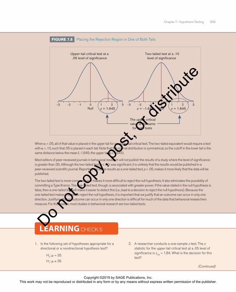
Kruger and Savitsky (2006) conducted a study in which they performed two tests on the same data. They completed an upper-tail critical test at α = .05 and a two-tailed test at α = .10. As shown in Figure 7.8, these are similar tests, except in the upper-tail test, all the alpha level is placed in the upper tail, and in the two-tailed test, the alpha level is split so that .05 is placed in each tail. When the researchers showed these results to a group of participants, they found that participants were more persuaded by a significant result when it was described as a one-tailed test, p < .05, than when it was described as a two-tailed test, p < .10. This was interesting because the two results were identical—both tests were associated with the same critical value in the upper tail.
Copyright ©2019 by SAGE Publications, Inc. This work may not be reproduced or distributed in any form or by any means without express written permission of the publisher.
Do not
copy
, pos
t, or d
istrib
ute
Chapter 7: Hypothesis Testing 209
When α = .05, all of that value is placed in the upper tail for an upper-tail critical test. The two-tailed equivalent would require a test with α = .10, such that .05 is placed in each tail. Note that the normal distribution is symmetrical, so the cutoff in the lower tail is the same distance below the mean (−1.645; the upper tail is +1.645).
Most editors of peer-reviewed journals in behavioral research will not publish the results of a study where the level of significance is greater than .05. Although the two-tailed test, p < .10, was significant, it is unlikely that the results would be published in a peer-reviewed scientific journal. Reporting the same results as a one-tailed test, p < .05, makes it more likely that the data will be published.
The two-tailed test is more conservative; it makes it more difficult to reject the null hypothesis. It also eliminates the possibility of committing a Type III error. The one-tailed test, though, is associated with greater power. If the value stated in the null hypothesis is false, then a one-tailed test will make it easier to detect this (i.e., lead to a decision to reject the null hypothesis). Because the one-tailed test makes it easier to reject the null hypothesis, it is important that we justify that an outcome can occur in only one direction. Justifying that an outcome can occur in only one direction is difficult for much of the data that behavioral researchers measure. For this reason, most studies in behavioral research are two-tailed tests.
FIGURE 7.8 Placing the Rejection Region in One of Both Tails
z = 1.645 z = −1.645
Upper-tail critical test at a.05 level of significance
Two-tailed test at a .10level of significance
The upper criticalvalue is the same
for both tests
0−1−2−3Null
21 3z = 1.645
0−1−2−3Null
21 3
LEARNING CHECK 5
1. Is the following set of hypotheses appropriate for a directional or a nondirectional hypothesis test?
H0: µ = 35
H1: µ ≠ 35
2. A researcher conducts a one-sample z test. The z statistic for the upper-tail critical test at a .05 level of significance is zobt = 1.84. What is the decision for this test?
(Continued)
Copyright ©2019 by SAGE Publications, Inc. This work may not be reproduced or distributed in any form or by any means without express written permission of the publisher.
Do not
copy
, pos
t, or d
istrib
ute
210 Part II: Probability and the Foundations of Inferential Statistics
7.7 meaSurIng tHe SIze of an effect: coHen’S dA decision to reject the null hypothesis means that an effect is sig-nificant. For a one-sample test, an effect is the difference between a sample mean and the population mean stated in the null hypothesis. In Examples 7.1 and 7.2 we found a significant effect, meaning that the sample mean was significantly larger than the value stated in the null hypothesis. Hypothesis testing identifies whether or not an effect exists in a population. When a sample mean would be likely to occur if the null hypothesis were true (p > .05), we decide that an effect does not exist in a population; the effect is not significant. When a sample mean would be unlikely to occur if the null hypothesis were true (typically less than a 5% likelihood, p < .05), we decide that an effect does exist in a population; the effect is significant. Hypothesis testing does not, however, inform us of how big the effect is.
To determine the size of an effect, we compute effect size. There are two ways to calculate the size of an effect. We can determine
1. how far scores shifted in the population, and
2. the percent of variance that can be explained by a given variable.
Effect size is most meaningfully reported with significant effects when the decision was to reject the null hypothesis. If an effect is not significant, as in instances when we retain the null hypothesis, then we are concluding that an effect does not exist in a population. It makes little sense to com-pute the size of an effect that we just concluded does not exist. In this sec-tion, we describe how far scores shifted in the population using a measure of effect size called Cohen’s d.
Cohen’s d measures the number of standard deviations an effect is shifted above or below the population mean stated by the null hypothesis. The formula for Cohen’s d replaces the standard error in the denominator of the test statistic with the population standard deviation (J. Cohen, 1988):
Cohen’s d M= −µσ
.
3. A researcher conducts a hypothesis test and finds that p = .0689. What is the decision for a hypothesis test at a .05 level of significance?
4. Which type of test, one-tailed or two-tailed, is susceptible to the possibility of committing a Type III error?
Answers: 1. A nondirectional (two-tailed) test; 2. Reject the null hypothesis; 3. Retain the null hypothesis; 4. One-tailed test.
(Continued)
For a single sample, an effect is the difference between a sample mean and the population mean stated in the null hypothesis. In hypothesis testing, an effect is not significant when we retain the null hypothesis; an effect is significant when we reject the null hypothesis.
Effect size is a statistical measure of the size of an effect in a population, which allows researchers to describe how far scores shifted in the population, or the percent of variance that can be explained by a given variable.
Cohen’s d is a measure of effect size in terms of the number of standard deviations that mean scores shifted above or below the population mean stated by the null hypothesis. The larger the value of d, the larger the effect in the population.
Copyright ©2019 by SAGE Publications, Inc. This work may not be reproduced or distributed in any form or by any means without express written permission of the publisher.
Do not
copy
, pos
t, or d
istrib
ute
Chapter 7: Hypothesis Testing 211
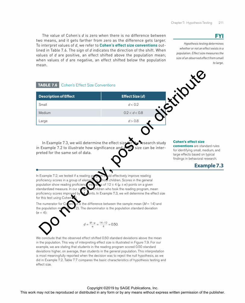
The value of Cohen’s d is zero when there is no difference between two means, and it gets farther from zero as the difference gets larger. To interpret values of d, we refer to Cohen’s effect size conventions out-lined in Table 7.6. The sign of d indicates the direction of the shift. When values of d are positive, an effect shifted above the population mean; when values of d are negative, an effect shifted below the population mean.
FYIHypothesis testing determines
whether or not an effect exists in a population. Effect size measures the size of an observed effect from small
to large.
TABLE 7.6 Cohen’s Effect Size Conventions
Description of Effect Effect Size (d)
Small d < 0.2
Medium 0.2 < d < 0.8
Large d > 0.8
In Example 7.3, we will determine the effect size for the research study in Example 7.2 to illustrate how significance and effect size can be inter-preted for the same set of data.
Example 7.3
In Example 7.2, we tested if a reading program could effectively improve reading proficiency scores in a group of elementary school children. Scores in the general population show reading proficiency increases of 12 ± 4 (µ ± σ) points on a given standardized measure. In our sample of children who took the reading program, mean proficiency scores improved by 14 points. In Example 7.3, we will determine the effect size for this test using Cohen’s d.
The numerator for Cohen’s d is the difference between the sample mean (M = 14) and the population mean (µ = 12). The denominator is the population standard deviation (σ = 4):
d M= = =− −µσ
14 124
0.50.
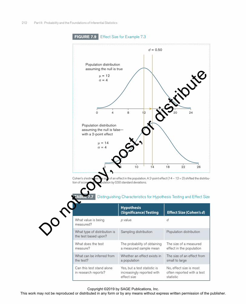
We conclude that the observed effect shifted 0.50 standard deviations above the mean in the population. This way of interpreting effect size is illustrated in Figure 7.9. For our example, we are stating that students in the reading program scored 0.50 standard deviations higher, on average, than students in the general population. This interpretation is most meaningfully reported when the decision was to reject the null hypothesis, as we did in Example 7.2. Table 7.7 compares the basic characteristics of hypothesis testing and effect size.
Cohen’s effect size conventions are standard rules for identifying small, medium, and large effects based on typical findings in behavioral research.
Copyright ©2019 by SAGE Publications, Inc. This work may not be reproduced or distributed in any form or by any means without express written permission of the publisher.
Do not
copy
, pos
t, or d
istrib
ute
212 Part II: Probability and the Foundations of Inferential Statistics
FIGURE 7.9 Effect Size for Example 7.3
Population distribution assuming the null is false—with a 2-point effect
d = 0.50
Population distributionassuming the null is true
µ = 12σ = 4
µ = 14σ = 4
0 4 8 16 20 24
2 6 10 18 22 26
12
14
Cohen’s d estimates the size of an effect in the population. A 2-point effect (14 − 12 = 2) shifted the distribu-tion of scores in the population by 0.50 standard deviations.
TABLE 7.7 Distinguishing Characteristics for Hypothesis Testing and Effect Size
Hypothesis (Significance) Testing Effect Size (Cohen’s d)
What value is being measured?
p value d
What type of distribution is the test based upon?
Sampling distribution Population distribution
What does the test measure?
The probability of obtaining a measured sample mean
The size of a measured effect in the population
What can be inferred from the test?
Whether an effect exists in a population
The size of an effect from small to large
Can this test stand alone in research reports?
Yes, but a test statistic is increasingly reported with effect size
No, effect size is most often reported with a test statistic
Copyright ©2019 by SAGE Publications, Inc. This work may not be reproduced or distributed in any form or by any means without express written permission of the publisher.
Do not
copy
, pos
t, or d
istrib
ute
Chapter 7: Hypothesis Testing 213
7.8 effect SIze, power, and Sample SIzeOne advantage of knowing effect size, d, is that its value can be used to determine the power of detecting an effect in hypothesis testing. The likelihood of detecting an effect, called power, is critical in behavioral research because it lets the researcher know the probability that a ran-domly selected sample will lead to a decision to reject the null hypothesis, if the null hypothesis is false. In this section, we describe how effect size and sample size are related to power.
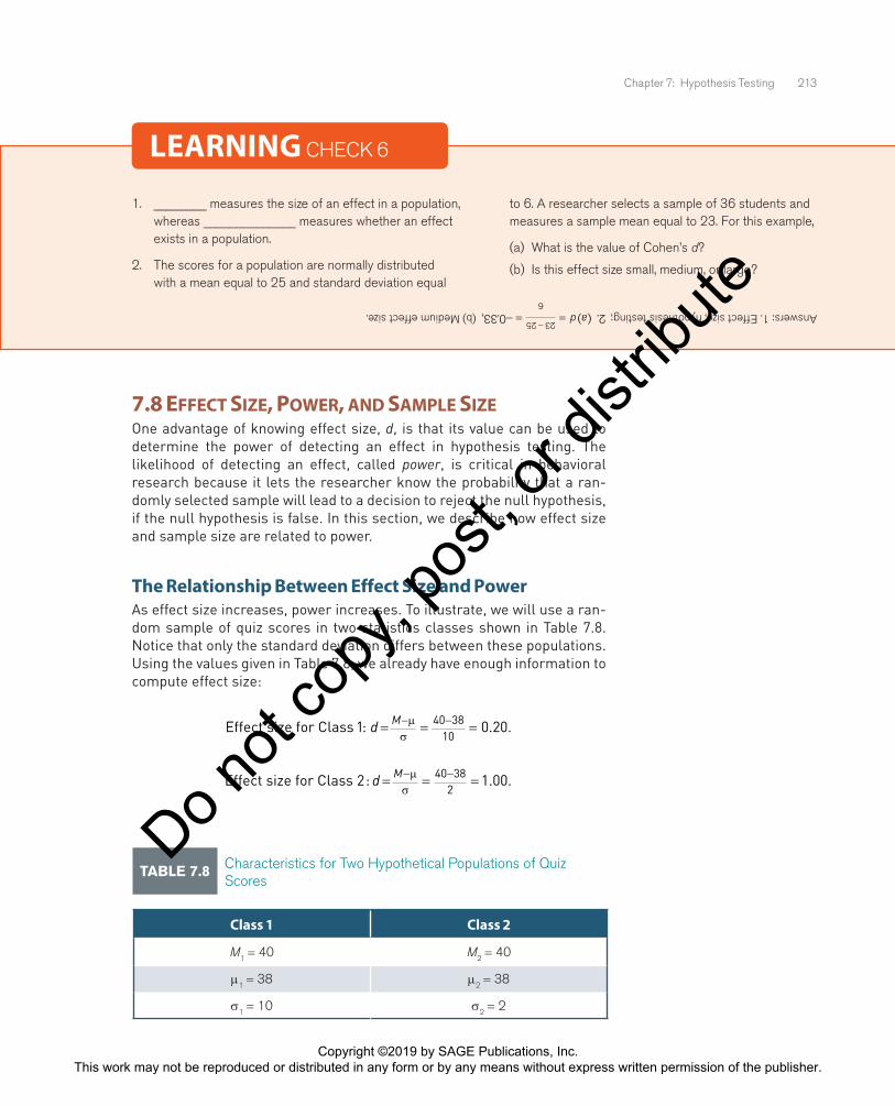
The Relationship Between Effect Size and PowerAs effect size increases, power increases. To illustrate, we will use a ran-dom sample of quiz scores in two statistics classes shown in Table 7.8. Notice that only the standard deviation differs between these populations. Using the values given in Table 7.8, we already have enough information to compute effect size:
Effect size for Class :1 0.2038d M= = =− −µσ
4010
.
Effect size for Class 2: d M= = =− −µσ
40 382
1 00. .
LEARNING CHECK 6
1. ________ measures the size of an effect in a population, whereas ______________ measures whether an effect exists in a population.
2. The scores for a population are normally distributed with a mean equal to 25 and standard deviation equal
to 6. A researcher selects a sample of 36 students and measures a sample mean equal to 23. For this example,
(a) What is the value of Cohen’s d?
(b) Is this effect size small, medium, or large?
Answers: 1. Effect size, hypothesis testing; 2.()0.33,2325
6ad==−
− (b) Medium effect size.
TABLE 7.8 Characteristics for Two Hypothetical Populations of Quiz Scores
Class 1 Class 2
M1 = 40 M2 = 40
µ1 = 38 µ2 = 38
σ1 = 10 σ2 = 2
Copyright ©2019 by SAGE Publications, Inc. This work may not be reproduced or distributed in any form or by any means without express written permission of the publisher.
Do not
copy
, pos
t, or d
istrib
ute
214 Part II: Probability and the Foundations of Inferential Statistics
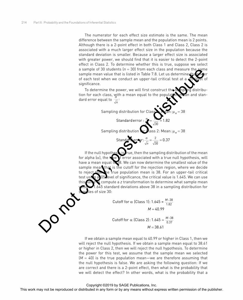
The numerator for each effect size estimate is the same. The mean difference between the sample mean and the population mean is 2 points. Although there is a 2-point effect in both Class 1 and Class 2, Class 2 is associated with a much larger effect size in the population because the standard deviation is smaller. Because a larger effect size is associated with greater power, we should find that it is easier to detect the 2-point effect in Class 2. To determine whether this is true, suppose we select a sample of 30 students (n = 30) from each class and measure the same sample mean value that is listed in Table 7.8. Let us determine the power of each test when we conduct an upper-tail critical test at a .05 level of significance.
To determine the power, we will first construct the sampling distribu-tion for each class, with a mean equal to the population mean and stan-dard error equal to
σ
n:
Sampling distribution for Class 1: Mean: µM = 38
Standard error : 1.8210
30
σ
n= =
Sampling distribution for Class 2: Mean: µM = 38
Standard error: σ
n= =2 0.37
30
If the null hypothesis is true, then the sampling distribution of the mean for alpha (α), the type of error associated with a true null hypothesis, will have a mean equal to 38. We can now determine the smallest value of the sample mean that is the cutoff for the rejection region, where we decide to reject that the true population mean is 38. For an upper-tail critical test using a .05 level of significance, the critical value is 1.645. We can use this value to compute a z transformation to determine what sample mean value is 1.645 standard deviations above 38 in a sampling distribution for samples of size 30:
Cutoff for (Class 1): 1.645 =α M
M
−
=
381 82
40 99.
.
Cutoff for Class : 1.645
38.61
38 ( 2)α =
=
M
M
−0 37.
If we obtain a sample mean equal to 40.99 or higher in Class 1, then we will reject the null hypothesis. If we obtain a sample mean equal to 38.61 or higher in Class 2, then we will reject the null hypothesis. To determine the power for this test, we assume that the sample mean we selected (M = 40) is the true population mean—we are therefore assuming that the null hypothesis is false. We are asking the following question: If we are correct and there is a 2-point effect, then what is the probability that we will detect the effect? In other words, what is the probability that a
Copyright ©2019 by SAGE Publications, Inc. This work may not be reproduced or distributed in any form or by any means without express written permission of the publisher.
Do not
copy
, pos
t, or d
istrib
ute
Chapter 7: Hypothesis Testing 215
sample randomly selected from this population will lead to a decision to reject the null hypothesis?
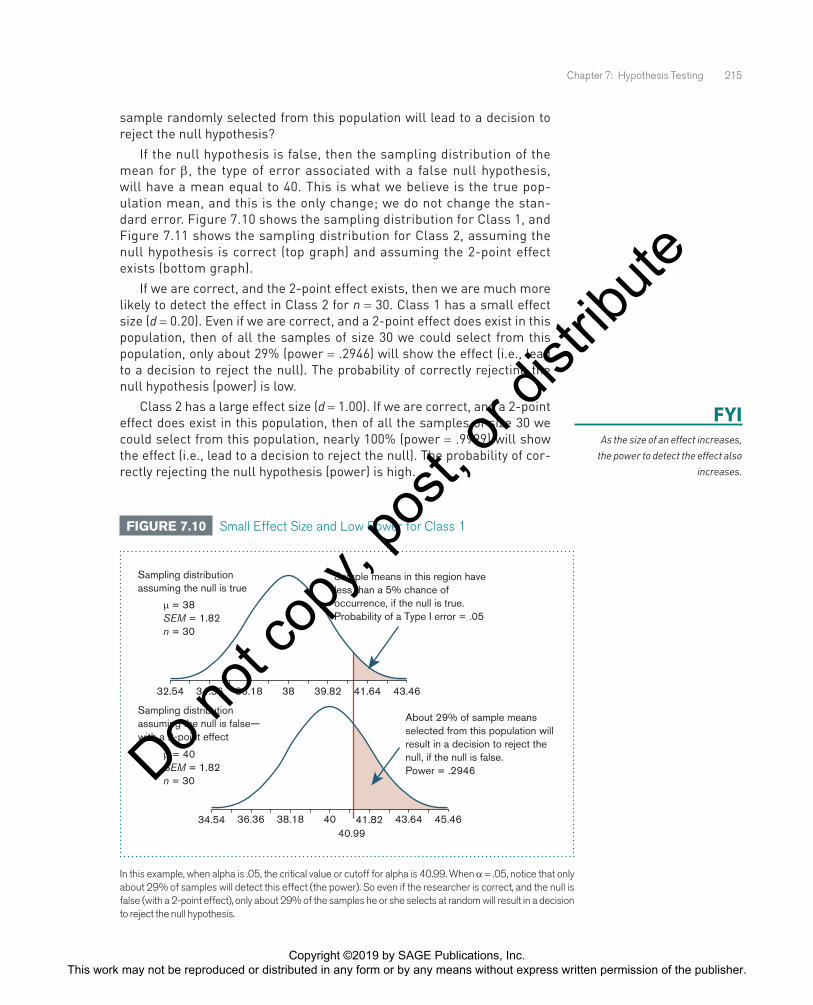
If the null hypothesis is false, then the sampling distribution of the mean for β, the type of error associated with a false null hypothesis, will have a mean equal to 40. This is what we believe is the true pop-ulation mean, and this is the only change; we do not change the stan-dard error. Figure 7.10 shows the sampling distribution for Class 1, and Figure 7.11 shows the sampling distribution for Class 2, assuming the null hypothesis is correct (top graph) and assuming the 2-point effect exists (bottom graph).
If we are correct, and the 2-point effect exists, then we are much more likely to detect the effect in Class 2 for n = 30. Class 1 has a small effect size (d = 0.20). Even if we are correct, and a 2-point effect does exist in this population, then of all the samples of size 30 we could select from this population, only about 29% (power = .2946) will show the effect (i.e., lead to a decision to reject the null). The probability of correctly rejecting the null hypothesis (power) is low.
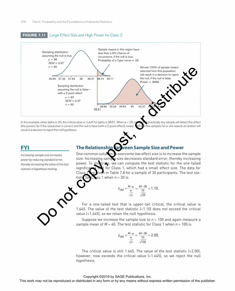
Class 2 has a large effect size (d = 1.00). If we are correct, and a 2-point effect does exist in this population, then of all the samples of size 30 we could select from this population, nearly 100% (power = .9999) will show the effect (i.e., lead to a decision to reject the null). The probability of cor-rectly rejecting the null hypothesis (power) is high.
FYIAs the size of an effect increases,
the power to detect the effect also increases.
FIGURE 7.10 Small Effect Size and Low Power for Class 1
Sample means in this region have less than a 5% chance of occurrence, if the null is true. Probability of a Type I error = .05
About 29% of sample means selected from this population will result in a decision to reject the null, if the null is false. Power = .2946
Sampling distribution assuming the null is false—with a 2-point effect
Sampling distributionassuming the null is true
µ = 38SEM = 1.82 n = 30
µ = 40SEM = 1.82n = 30
32.54 34.36 36.18 38 39.82 41.64 43.46
4040.99
41.82 43.64 45.4634.54 36.36 38.18
In this example, when alpha is .05, the critical value or cutoff for alpha is 40.99. When α = .05, notice that only about 29% of samples will detect this effect (the power). So even if the researcher is correct, and the null is false (with a 2-point effect), only about 29% of the samples he or she selects at random will result in a decision to reject the null hypothesis.
Copyright ©2019 by SAGE Publications, Inc. This work may not be reproduced or distributed in any form or by any means without express written permission of the publisher.
Do not
copy
, pos
t, or d
istrib
ute
216 Part II: Probability and the Foundations of Inferential Statistics
The Relationship Between Sample Size and PowerOne common solution to overcome low effect size is to increase the sample size. Increasing sample size decreases standard error, thereby increasing power. To illustrate, we can compute the test statistic for the one-tailed significance test for Class 1, which had a small effect size. The data for Class 1 are given in Table 7.8 for a sample of 30 participants. The test sta-tistic for Class 1 when n = 30 is
z M
n
obt 1.10.= = =− −µσ
40 3810
30
For a one-tailed test that is upper-tail critical, the critical value is 1.645. The value of the test statistic (+1.10) does not exceed the critical value (+1.645), so we retain the null hypothesis.
Suppose we increase the sample size to n = 100 and again measure a sample mean of M = 40. The test statistic for Class 1 when n = 100 is
z M
n
obt 2.00= = =− −µσ
40 3810
100
.
The critical value is still 1.645. The value of the test statistic (+2.00), however, now exceeds the critical value (+1.645), so we reject the null hypothesis.
FIGURE 7.11 Large Effect Size and High Power for Class 2
Sample means in this region have less than a 5% chance of occurrence, if the null is true. Probability of a Type I error = .05
Almost 100% of sample means selected from this population will result in a decision to reject the null, if the null is false. Power = .9999
Sampling distribution assuming the null is false—with a 2-point effect
Sampling distributionassuming the null is true
µ = 38SEM = 0.37n = 30
µ = 40SEM = 0.37n = 30
36.89 37.26 37.63 38 38.37 39.11
40 40.37 40.74 41.1138.8938.61
39.26 39.63
38.74
In this example, when alpha is .05, the critical value or cutoff for alpha is 38.61. When α = .05, notice that practically any sample will detect this effect (the power). So if the researcher is correct, and the null is false (with a 2-point effect), nearly 100% of the samples he or she selects at random will result in a decision to reject the null hypothesis.
FYIIncreasing sample size increases power by reducing standard error, thereby increasing the value of the test statistic in hypothesis testing.
Copyright ©2019 by SAGE Publications, Inc. This work may not be reproduced or distributed in any form or by any means without express written permission of the publisher.
Do not
copy
, pos
t, or d
istrib
ute

Chapter 7: Hypothesis Testing 217
Notice that increasing the sample size alone led to a decision to reject the null hypothesis, despite testing for a small effect size in the popu-lation. Hence, increasing sample size increases power: It makes it more likely that we will detect an effect, assuming that an effect exists in a given population.
LEARNING CHECK 7
1. As effect size increases, what happens to the power?
2. As effect size decreases, what happens to the power?
3. When a population is associated with a small effect size, what can a researcher do to increase the power of the study?
4. True or false: The effect size, power, and sample size of a study can affect the decisions we make in hypothesis testing.
Answers: 1. Power increases; 2. Power decreases; 3. Increase the sample size (n); 4. True.
7.9 addItIonal factorS tHat IncreaSe powerThe power is the likelihood of detecting an effect. Behavioral research often requires a great deal of time and money to select, observe, measure, and analyze data. For this reason, the institutions that offer substantial funding for research studies want to know that they are spending their money wisely and that researchers conduct studies that will show results. Consequently, to receive a research grant, researchers are often required to state the likelihood that they will detect an effect they are studying, assuming they are correct. In other words, researchers must disclose the power of their studies.
The typical standard for power is .80. Researchers try to make sure that at least 80% of the samples they select will show an effect when an effect exists in a population. In Section 7.8, we showed that increasing effect size and sample size increases power. In this section, we introduce four additional factors that influence power.
Increasing Power: Increase Effect Size, Sample Size, and AlphaIncreasing effect size, sample size, and the alpha level will increase power. Section 7.8 showed that increasing effect size and sample size increases power; here we discuss increasing alpha. The alpha level is the probability of a Type I error, and it is the rejection region for a hypothesis test. The larger the rejection region, the greater the likelihood of rejecting the null hypothesis, and the greater the power will be. Hence, increasing the size
FYITo increase power, increase effect size,
sample size, and alpha; and decrease beta, population standard deviation,
and standard error.
Copyright ©2019 by SAGE Publications, Inc. This work may not be reproduced or distributed in any form or by any means without express written permission of the publisher.
Do not
copy
, pos
t, or d
istrib
ute
218 Part II: Probability and the Foundations of Inferential Statistics
of the rejection region in the upper tail in Example 7.2 (by placing all of the rejection region in one tail) increased the power of that hypothesis test. Similarly, increasing alpha will increase the size of the rejection region, thereby increasing power. That being said, it is widely accepted that alpha can never be stated at a value larger than .05. Simply increasing alpha is not a practical solution to increase power. Instead, the more practical solutions are to increase sample size, or structure your study to observe a large effect between groups.
Increasing Power: Decrease Beta, Standard Deviation (σ), and Standard ErrorDecreasing beta error (β) increases power. In Table 7.3, β is given as the probability of a Type II error, and 1 − β is given as the power. The lower β is, the greater the solution will be for 1 − β. For example, say β = .20. In this case, 1 − β = (1 − .20) = .80. If we decrease β, say, to β = .10, the power will increase: 1 − β = (1 − .10) = .90. Hence, decreasing beta error increases power.
Decreasing the population standard deviation (σ) and standard error (σM) will also increase power. The population standard deviation is the numerator for computing standard error. Decreasing the population stan-dard deviation will decrease the standard error, thereby increasing the value of the test statistic. To illustrate, suppose that we select a sample from a population of students with quiz scores equal to 10 ± 8 (µ ± σ). We select a sample of 16 students from this population and measure a sample mean equal to 12. In this example, the standard error is
σ σM
n= = =8
162 00. .
To compute the z statistic, we subtract the sample mean from the pop-ulation mean and divide by the standard error:
z M
Mobt
12 1.00.= = =− −µσ
102
An obtained value equal to 1.00 does not exceed the critical value for a one-tailed test (critical value = 1.645) or a two-tailed test (critical values = ±1.96). The decision is to retain the null hypothesis.
If the population standard deviation is smaller, the standard error will be smaller, thereby making the value of the test statistic larger. Suppose, for example, that we reduce the population standard deviation to 4. The standard error in this example is now
σ σM
n= = =4
161.0.
To compute the z statistic, we subtract the sample mean from the pop-ulation mean and divide by this smaller standard error:
z M
Mobt = = =− −µ
σ12 10
12 00. .
Copyright ©2019 by SAGE Publications, Inc. This work may not be reproduced or distributed in any form or by any means without express written permission of the publisher.
Do not
copy
, pos
t, or d
istrib
ute
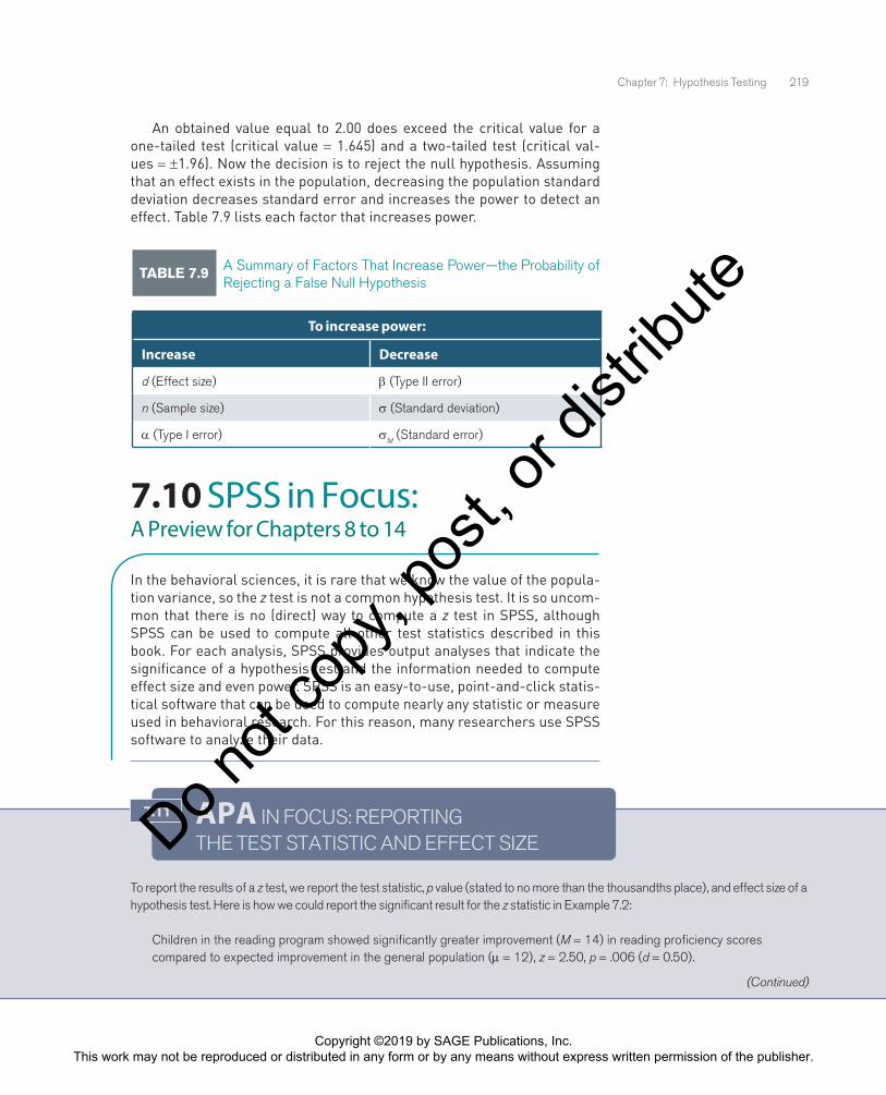
Chapter 7: Hypothesis Testing 219
7.11 APA IN FOCUS: REPORTING THE TEST STATISTIC AND EFFECT SIZE
To report the results of a z test, we report the test statistic, p value (stated to no more than the thousandths place), and effect size of a hypothesis test. Here is how we could report the significant result for the z statistic in Example 7.2:
Children in the reading program showed significantly greater improvement (M = 14) in reading proficiency scores compared to expected improvement in the general population (µ = 12), z = 2.50, p = .006 (d = 0.50).
An obtained value equal to 2.00 does exceed the critical value for a one-tailed test (critical value = 1.645) and a two-tailed test (critical val-ues = ±1.96). Now the decision is to reject the null hypothesis. Assuming that an effect exists in the population, decreasing the population standard deviation decreases standard error and increases the power to detect an effect. Table 7.9 lists each factor that increases power.
TABLE 7.9 A Summary of Factors That Increase Power—the Probability of Rejecting a False Null Hypothesis
To increase power:
Increase Decrease
d (Effect size) β (Type II error)
n (Sample size) σ (Standard deviation)
α (Type I error) σM (Standard error)
7.10 SPSS in Focus: A Preview for Chapters 8 to 14
In the behavioral sciences, it is rare that we know the value of the popula-tion variance, so the z test is not a common hypothesis test. It is so uncom-mon that there is no (direct) way to compute a z test in SPSS, although SPSS can be used to compute all other test statistics described in this book. For each analysis, SPSS provides output analyses that indicate the significance of a hypothesis test and the information needed to compute effect size and even power. SPSS is an easy-to-use, point-and-click statis-tical software that can be used to compute nearly any statistic or measure used in behavioral research. For this reason, many researchers use SPSS software to analyze their data.
(Continued)
Copyright ©2019 by SAGE Publications, Inc. This work may not be reproduced or distributed in any form or by any means without express written permission of the publisher.
Do not
copy
, pos
t, or d
istrib
ute
220 Part II: Probability and the Foundations of Inferential Statistics
Notice that when we report a result, we do not state that we reject or retain the null hypothesis. Instead, we report whether a result is significant (the decision was to reject the null hypothesis) or not significant (the decision was to retain the null hypothesis). Also, you are not required to report the exact p value, although it is recommended. An alternative is to report it in terms of p < .05, p < .01, or p < .001. In our example, we could state p < .01 for a p value actually equal to .006.
Finally, notice that the means are also listed in the summary of the data. Often we can also report standard deviations, which is recommended by the APA. An alternative would be to report the means in a figure or table to illustrate a significant effect, with error bars given in a figure to indicate the standard error of the mean. In this way, we can report the value of the test statistic, p value, effect size, means, standard deviations, and standard error all in one sentence and a figure or table.
(Continued)
cHapter Summary organIzed by learnIng objectIve
LO 1: Identify the four steps of hypothesis testing.• Hypothesis testing, or significance
testing, is a method of testing a claim or hypothesis about a parameter in a population, using data measured in a sample. In this method, we test a hypothesis by determining the likeli-hood that a sample statistic would be selected if the hypothesis regarding the population parameter were true. The four steps of hypothesis testing are as follows:
Step 1: State the hypotheses.
Step 2: Set the criteria for a decision.
Step 3: Compute the test statistic.
Step 4: Make a decision.
LO 2: Define null hypothesis, alternative hypothesis, level of significance, test statistic, p value, and statistical significance.
• The null hypothesis (H0) is a state-ment about a population parameter, such as the population mean, that is assumed to be true.
• The alternative hypothesis (H1) is a statement that directly contradicts a null hypothesis by stating that the
actual value of a population param-eter, such as the mean, is less than, greater than, or not equal to the value stated in the null hypothesis.
• Level of significance is a criterion of judgment upon which a decision is made regarding the value stated in a null hypothesis. The criterion is based on the probability of obtaining a statistic measured in a sample if the value stated in the null hypothe-sis were true.
• The test statistic is a mathematical formula that allows researchers to determine the likelihood or proba-bility of obtaining sample outcomes if the null hypothesis were true. The value of a test statistic can be used to make inferences concerning the value of a population parameter stated in the null hypothesis.
• A p value is the probability of obtain-ing a sample outcome, given that the value stated in the null hypoth-esis is true. The p value of a sample outcome is compared to the level of significance.
• Significance, or statistical signifi-cance, describes a decision made
Copyright ©2019 by SAGE Publications, Inc. This work may not be reproduced or distributed in any form or by any means without express written permission of the publisher.
Do not
copy
, pos
t, or d
istrib
ute
Chapter 7: Hypothesis Testing 221
concerning a value stated in the null hypothesis. When a null hypothesis is rejected, a result is significant. When a null hypothesis is retained, a result is not significant.
LO 3: Define Type I error and Type II error, and identify the type of error that researchers control.• We can decide to retain or reject a
null hypothesis, and this decision can be correct or incorrect. Two types of errors in hypothesis testing are called Type I and Type II errors.
• A Type I error is the probability of rejecting a null hypothesis that is actually true. The probability of this type of error is determined by the researcher and stated as the level of significance or alpha level for a hypothesis test.
• A Type II error is the probability of retaining a null hypothesis that is actually false.
LO 4: Calculate the one-sample z test and interpret the results.• The one-sample z test is a statisti-
cal procedure used to test hypothe-ses concerning the mean in a single population with a known variance. The test statistic for this hypothesis test is
z M
MM
nobt ,where= =−µ
σσσ .
• Critical values, which mark the cut-offs for the rejection region, can be identified for any level of signifi-cance. The value of the test statistic is compared to the critical values. When the value of a test statistic exceeds a critical value, we reject the null hypothesis; otherwise, we retain the null hypothesis.
LO 5: Distinguish between a one-tailed test and two-tailed test, and explain why a Type III error is possible only with one-tailed tests.
• Nondirectional (two-tailed) tests are hypothesis tests in which the alter-native hypothesis is stated as not equal to (≠) a value stated in the null hypothesis. So we are interested in any alternative to the null hypothesis.
• Directional (one-tailed) tests are hypothesis tests in which the alter-native hypothesis is stated as greater than (>) or less than (<) a value stated in the null hypothesis. So we are interested in a specific alternative to the null hypothesis.
• A Type III error is a type of error pos-sible with one-tailed tests in which a result would have been signifi-cant in one tail, but the researcher retains the null hypothesis because the rejection region was placed in the wrong or opposite tail.
LO 6: Elucidate effect size and compute a Cohen’s d for the one-sample z test.• Effect size is a statistical measure
of the size of an observed effect in a population, which allows research-ers to describe how far scores shifted in the population, or the percent of variance that can be explained by a given variable.
• Cohen’s d is used to measure how far scores shifted in a population and is computed using the following formula:
Cohen’s d M= −µσ
.
• To interpret the size of an effect, we refer to Cohen’s effect size conven-tions, which are standard rules for identifying small, medium, and large effects based on typical findings in behavioral research. These conven-tions are given in Table 7.6.
LO 7: Define power and identify six factors that influence power.• In hypothesis testing, power is the
probability that a sample selected
Copyright ©2019 by SAGE Publications, Inc. This work may not be reproduced or distributed in any form or by any means without express written permission of the publisher.
Do not
copy
, pos
t, or d
istrib
ute

222 Part II: Probability and the Foundations of Inferential Statistics
at random will show that the null hypothesis is false when the null hypothesis is indeed false.
• To increase the power of detecting an effect in a given population:
a. Increase effect size (d), sample size (n), and alpha (α).
b. Decrease beta error (β), popula-tion standard deviation (σ), and standard error (σM).
LO 8: Summarize the results of a one-sample z test in APA format.• To report the results of a z test, we
report the test statistic, p value, and effect size of a hypothesis test. In addition, a figure or table can be used to summarize the means and standard error or standard deviation measured in a study.
key termSalpha (α) levelalternative hypothesis (H1)beta (β) errorCohen’s dCohen’s effect size conventionscritical valuedirectional testseffecteffect sizehypothesis
hypothesis testinglevel of significancenondirectional testsnull hypothesis (H0)obtained valueone-sample z testone-tailed testp valuepowerrejection region
significancesignificance levelsignificance testingstatistical significancetest statistictwo-tailed testsType I errorType II errorType III errorz statistic
end-of-cHapter problemS
Factual Problems
1. State the four steps of hypothesis testing.
2. What are two decisions that a researcher makes in hypothesis testing?
3. What is the power in hypothesis testing?
4. What is a Type II error (β)?
5. What is a Type I error (α)?
6. What are the critical values for a one-sample nondirectional (two-tailed) z test at a .05 level of significance?
7. Is a one-tailed test associated with greater power than a two-tailed test? Explain.
8. How are the rejection regions, the probability of a Type I error, the level of significance, and the alpha level related?
9. Alpha (α) is used to measure the error for deci-sions concerning true null hypotheses. What is beta (β) error used to measure?
10. What three factors can be decreased to increase power?
11. What three factors can be increased to increase power?
12. Distinguish between the significance and the effect size of a result.
Concept and Application Problems
13. A researcher conducts a hypothesis test and concludes that his hypothesis is correct. Explain why this conclusion is never an appro-priate decision in hypothesis testing.
14. Explain why the following statement is true: The population standard deviation is always larger than the standard error when the sam-ple size is greater than one (n > 1).
Copyright ©2019 by SAGE Publications, Inc. This work may not be reproduced or distributed in any form or by any means without express written permission of the publisher.
Do not
copy
, pos
t, or d
istrib
ute
Chapter 7: Hypothesis Testing 223
15. The weight (in pounds) for a population of school-aged children is normally distributed with a mean equal to 135 ± 20 pounds (µ ± σ). Suppose we select a sample of 100 children (n = 100) to test whether children in this pop-ulation are gaining weight at a .05 level of significance.
(a) What is the null hypothesis? What is the alternative hypothesis?
(b) What is the critical value for this test?
(c) What is the mean of the sampling distribution?
(d) What is the standard error of the mean for the sampling distribution?
16. A researcher selects a sample of 30 partic-ipants and makes the decision to retain the null hypothesis. She conducts the same study testing the same hypothesis with a sample of 300 participants and makes the decision to reject the null hypothesis. Give a likely expla-nation for why the two samples led to different decisions.
17. A researcher conducts a one-sample z test and makes the decision to reject the null hypothe-sis. Another researcher selects a larger sam-ple from the same population, obtains the same sample mean, and makes the decision to retain the null hypothesis using the same hypothesis test. Is this possible? Explain.
18. Determine the level of significance for a hypothesis test in each of the following popu-lations given the specified standard error and critical values. Hint: Refer to the values given in Table 7.4:
(a) µ = 100, σM = 8, critical values: 84.32 and 115.68
(b) µ = 100, σM = 6, critical value: 113.98
(c) µ = 100, σM = 4, critical value: 86.8
19. For each p value stated below, (1) what is the decision for each if α = .05, and (2) what is the decision for each if α = .01?
(a) p = .1000
(b) p = .0050
(c) p = .0250
(d) p = .0001
20. For each obtained value stated below, (1) what is the decision for each if α = .05 (one-tailed test, upper-tail critical), and (2) what is the decision for each if α = .01 (two-tailed test)?
(a) zobt = 2.10
(b) zobt = 1.70
(c) zobt = 2.75
(d) zobt = −3.30
21. Will each of the following increase, decrease, or have no effect on the value of a test statistic for the one-sample z test?
(a) The sample size is increased.
(b) The sample variance is doubled.
(c) The population variance is decreased.
(d) The difference between the sample mean and population mean is decreased.
22. The physical fitness score for a population of police officers at a local police station is 72, with a standard deviation of 7 on a 100-point physical endurance scale. Suppose the police chief selects a sample of 49 local police offi-cers from this population and records a mean physical fitness rating on this scale equal to 74. He conducts a one-sample z test to deter-mine whether physical endurance increased at a .05 level of significance.
(a) State the value of the test statistic and whether to retain or reject the null hypothesis.
(b) Compute effect size using Cohen’s d.
23. A national firm reports mean earnings of $75 ± $12 (µ ± σ) per unit sold over the lifetime of the company. A competing company over the past 36 reporting periods had reported mean earnings equal to $78 per unit sold. Conduct a one-sample z test to determine whether mean earnings (in dollars per unit) are larger (com-pared to that reported by the national firm) at a .05 level of significance.
(a) State the value of the test statistic and whether to retain or reject the null hypothesis.
(b) Compute effect size using Cohen’s d.
24. A local school reports that the average grade point average (GPA) in the entire school is
Copyright ©2019 by SAGE Publications, Inc. This work may not be reproduced or distributed in any form or by any means without express written permission of the publisher.
Do not
copy
, pos
t, or d
istrib
ute
224 Part II: Probability and the Foundations of Inferential Statistics
a mean score of 2.66, with a standard devia-tion of 0.40. The school announces that it will be introducing a new program designed to improve GPA scores at the school. What is the effect size (d) for this program if it is expected to improve GPA by:
(a) 0.05 points?
(b) 0.10 points?
(c) 0.40 points?
25. Will each of the following increase, decrease, or have no effect on the value of Cohen’s d?
(a) The population variance is increased.
(b) The sample size is decreased.
(c) The sample variance is reduced.
(d) The difference between the sample and population mean is increased.
26. State whether the effect size for a 1-point effect (M − µ = 1) is small, medium, or large given the following population variances:
(a) σ = 1
(b) σ = 2
(c) σ = 4
(d) σ = 6
27. As α increases, so does the power to detect an effect. Why, then, do we restrict α from being larger than .05?
28. Will increasing sample size (n) increase or decrease the value of standard error? Will this increase or decrease power?
Problems in Research
29. Directional versus nondirectional hypothesis testing. Cho and Abe (2013) provided a com-mentary on the appropriate use of one-tailed and two-tailed tests in behavioral research. In their discussion, they outlined the following hypothetical null and alternative hypotheses to test a research hypothesis that males self-disclose more than females:
H0: µmales – µfemales ≤ 0
H1: µmales – µfemales > 0
(a) What type of test is set up with these hypotheses, a directional test or a nondi-rectional test?
(b) Do these hypotheses encompass all possi-bilities for the population mean? Explain.
30. The one-tailed tests. In their book, Common Errors in Statistics (and How to Avoid Them), Good and Hardin (2003) wrote, “No one will know whether your [one-tailed] hypothesis was con-ceived before you started or only after you had examined the data” (p. 347). Why do the authors state this as a concern for one-tailed tests?
31. The value of a p value. In a critical commen-tary on the use of significance testing, Charles Lambdin (2012) explained, “If a p < .05 result is
‘significant,’ then a p = .067 result is not ‘mar-ginally significant’” (p. 76). Explain what the author is referring to in terms of the two deci-sions that a researcher can make.
32. Describing the z test. In an article describing hypothesis testing with small sample sizes, Collins and Morris (2008) provided the follow-ing description for a z test: “Z is considered sig-nificant if the difference is more than roughly two standard deviations above or below zero (or more precisely, |Z| > 1.96)” (p. 464). Based on this description,
(a) Are the authors referring to critical val-ues for a one-tailed z test or a two-tailed z test?
(b) What alpha level are the authors referring to?
33. Sample size and power. Davis and Loprinzi (2016) evaluated a hypothesis related to engag-ing children, adolescents, and adults in physi-cal activity. As part of their study, they reported a sample size of 106 children, 128 adolescents, and 440 adults. Assuming equal effect sizes across these age groups, which age group is likely to be associated with greater power to detect effects of physical activity? Explain.
Copyright ©2019 by SAGE Publications, Inc. This work may not be reproduced or distributed in any form or by any means without express written permission of the publisher.
Do not
copy
, pos
t, or d
istrib
ute

Chapter 7: Hypothesis Testing 225
34. Making decisions in hypothesis testing. Toll, Kroesbergen, and Van Luit (2016) tested their hypothesis regarding real math difficulties among children. In their study, the authors concluded: “Our hypothesis [regarding math
difficulties] was confirmed” (p. 429). In this example, what decision did the authors make: Retain or reject the null hypothesis?
Answers for even numbers are in Appendix D.
Sharpen your skills with SAGE edge at edge.sagepub.com/priviteraess2e
SAGE edge for Students provides a personalized approach to help you accomplish your coursework goals in an easy-to-use learning environment.
Copyright ©2019 by SAGE Publications, Inc. This work may not be reproduced or distributed in any form or by any means without express written permission of the publisher.
Do not
copy
, pos
t, or d
istrib
ute

cosmin4000/iStock/Thinkstock
Copyright ©2019 by SAGE Publications, Inc. This work may not be reproduced or distributed in any form or by any means without express written permission of the publisher.
Do not
copy
, pos
t, or d
istrib
ute