NeuroImage 63 (2012) 11–24

Contents lists available at SciVerse ScienceDirect

NeuroImage

j ourna l homepage: www.e lsev ie r .com/ locate /yn img

Significant correlation between a set of genetic polymorphisms and a functional brainnetwork revealed by feature selection and sparse Partial Least Squares

Édith Le Floch a,c,j,⁎, Vincent Guillemot a,c, Vincent Frouin a,c, Philippe Pinel b,c, Christophe Lalanne f,g,Laura Trinchera h, Arthur Tenenhaus i, Antonio Moreno b,c, Monica Zilbovicius c,k, Thomas Bourgeron e,Stanislas Dehaene b,c, l, Bertrand Thirion a,c,d, Jean-Baptiste Poline a,c,d,j, Édouard Duchesnay a,c,j

a Laboratoire de Neuroimagerie Assistée par Ordinateur, Neurospin Center, I2BM, DSV, CEA, Gif-sur-Yvette, Franceb Cognitive Neuroimaging Unit U992, INSERM-CEA, Neurospin Center, Gif-sur-Yvette, Francec Université Paris-Sud, IFR49, Institut d'Imagerie Neurofonctionnelle, Paris, Franced Parietal Project Team, INRIA Saclay-Ile de France, Neurospin Center, I2BM, DSV, CEA, Gif-sur-Yvette, Francee Institut Pasteur, Laboratoire de Génétique Humaine et Fonctions Cognitives, Paris, Francef INSERM U669, PSIGIAM, Paris, Franceg AP-HP, Department of Clinical Research, Saint-Louis Hospital, Parish AgroParisTech, UMR518 MIA, Paris, Francei Supélec, Department of Signal Processing and Electronic Systems, Gif-sur-Yvette, Francej INSERM-CEA U1000, Neuroimaging & Psychiatry Unit, SHFJ, Orsay, Francek INSERM-CEA U1000, Neuroimaging & Psychiatry Unit, Necker Hospital, Paris, Francel Collège de France, F-75005 Paris, France

⁎ Corresponding author at: CEA, Neurospin, LNGif-sur-Yvette, France.

E-mail address: edith.lefloch@gmail.com (É. Le Floch

1053-8119/$ – see front matter © 2012 Elsevier Inc. Alldoi:10.1016/j.neuroimage.2012.06.061

a b s t r a c t

a r t i c l e i n f o

Article history:Accepted 27 June 2012Available online 8 July 2012

Keywords:Multivariate genetic analysisPartial Least Squares regressionCanonical Correlation AnalysisFeature selectionRegularisation

Brain imaging is increasingly recognised as an intermediate phenotype to understand the complex path be-tween genetics and behavioural or clinical phenotypes. In this context, a first goal is to propose methods toidentify the part of genetic variability that explains some neuroimaging variability. Classical univariate ap-proaches often ignore the potential joint effects that may exist between genes or the potential covariationsbetween brain regions. In this paper, we propose instead to investigate an exploratory multivariate methodin order to identify a set of Single Nucleotide Polymorphisms (SNPs) covarying with a set of neuroimagingphenotypes derived from functional Magnetic Resonance Imaging (fMRI). Recently, Partial Least Squares(PLS) regression or Canonical Correlation Analysis (CCA) have been proposed to analyse DNA andtranscriptomics. Here, we propose to transpose this idea to the DNA vs. imaging context. However, in veryhigh-dimensional settings like in imaging genetics studies, such multivariate methods may encounteroverfitting issues. Thus we investigate the use of different strategies of regularisation and dimension reduc-tion techniques combined with PLS or CCA to face the very high dimensionality of imaging genetics studies.We propose a comparison study of the different strategies on a simulated dataset first and then on a realdataset composed of 94 subjects, around 600,000 SNPs and 34 functional MRI lateralisation indexes comput-ed from reading and speech comprehension contrast maps. We estimate the generalisability of the multivar-iate association with a cross-validation scheme and demonstrate the significance of this link, using apermutation procedure. Univariate selection appears to be necessary to reduce the dimensionality. However,the significant association uncovered by this two-step approach combining univariate filtering and L1-regularised PLS suggests that discovering meaningful genetic associations calls for a multivariate approach.

© 2012 Elsevier Inc. All rights reserved.

1. Introduction

Imaging genetics studies that include a large amount of data inboth the imaging and the genetic components are facing challengesfor which the neuroimaging community has no definitive answer so

AO, Bâtiment 145, F-91191

).

rights reserved.

far. Current imaging genetics studies are often either limiting thebrain imaging endophenotype studied to a few candidate variablesbut testing their relationship with a large number of Single Nucleo-tide Polymorphisms (SNPs) as one usually proceeds during genescreening (e.g., Furlanello et al., 2003), or limiting the number of can-didate SNPs or genes to be tested on the whole brain or some largeportion of it (e.g., Glahn et al., 2007; McAllister et al., 2006; Roffmanet al., 2006). When faced with both a large number of SNPs and alarge number of voxels, one has to design an appropriate analysis

12 É. Le Floch et al. / NeuroImage 63 (2012) 11–24

strategy that should be as sensitive and specific as possible. Withoutany priors on genetic or brain regions involved, exploratory methodscan be used. The simplest approach to exploratory imaging geneticsstudies is clearly to apply a massive univariate analysis on both genet-ic and imaging data (Stein et al., 2010), which may be calledMass-Univariate Linear Modelling (MULM). However, while univari-ate techniques are simpler, they encounter a multiple comparisonproblem in the order of 1011. Moreover, the link between geneticand imaging data is likely to be in part multivariate, as for instanceepistasis or pleiotropy are likely phenomena in common traits or dis-eases. Indeed, brain imaging endophenotypes are probably influencedby the combined effects of several SNPs and different brain regionsmay also be influenced by the same SNP(s). A way to partially takeinto account epistasis may be to use a gene-based method to testfor the joint effect of the different SNPs within each gene across thevoxels of the whole brain (Hibar et al., 2011).

In this work, we try to go further and to identify a functional brainnetwork covarying with a set of genetic polymorphisms, using somemultivariate methods that take into account potential joint effectsor covariations within each block of variables. Partial Least Squares(PLS) regression (Wold et al., 1983) and Canonical Correlation Analy-sis (CCA) (Hotelling, 1936) appear to be good candidates in order tolook for associations between two blocks of data, as they extractpairs of covarying/correlated latent variables (one linear combinationof the variables for each block). Another approach has also been pro-posed by Calhoun et al. (2009) based on parallel Independent Compo-nent Analysis in order to combine functional MRI data and SNPs fromcandidate regions. Nevertheless, all these multivariate methods en-counter critical overfitting issues due to the very high dimensionalityof the data.

To face these issues, methods based on dimension reduction orregularisation can be used.

Dimension reduction is essentially based on two paradigms: fea-ture extraction and feature selection. Feature extraction looks for alow-dimensional representation of the data that explains most of itsvariability, the transformation being either linear such as PrincipalComponents Analysis (PCA) or non-linear such as manifold learningmethods. Feature selection methods may be divided into two catego-ries: some univariate methods (filters), which select relevant featuresindependently from each other, and some multivariate methods,which consider feature inter-relations to select a subset of variables(Guyon et al., 2006).

As for regularisation, multivariate methods based on L1 and/or L2penalisations, like sparse Partial Least Squares (Chun and Keleş, 2010;Lê Cao et al., 2008, 2009; Parkhomenko et al., 2007, 2009;Waaijenborg et al., 2008; Witten and Tibshirani, 2009) or regularisedCCA (Soneson et al., 2010), have recently been shown to provide goodresults in correlating two blocks of data such as transcriptomic andmetabolomic data, gene expression levels and gene copy numbers,or gene expression levels and SNP data. One may note that suchsparse multivariate methods based on L1 penalisation actually per-form variable selection. Vounou et al. (2010) also introduced a prom-ising similar method, called sparse Reduced-Rank Regression (sRRR)and based on L1 penalisation, that they applied to a simulated datasetmade of 111 brain imaging features and 10s of 1000s of SNPs. The im-plementation of the method becomes equivalent to sparse PLS in highdimensional settings, since they make the classical approximationthat in this case the covariance matrix of each block may be replacedby its diagonal elements (see Appendix). However, whether thesemultivariate techniques can resist even higher dimensions remainsan open question. In this paper we investigate this question by addinga first step of dimension reduction on SNPs, either by PCA or univar-iate filtering, before applying (sparse) PLS or (regularised) CCA. Wefirst use a simulated dataset mimicking fMRI and genome-wide SNPdata and compare the performances of the different methods, byassessing their positive predictive value, as well as their capacity to

generalise the link found between the two blocks with a cross-validation procedure. Indeed, we first compared PLS and CCA, thenwe investigated the influence of L2 regularisation on CCA and L1regularisation on PLS, and finally we tried to add a first step of dimen-sion reduction such as PCA or filtering.

Finally, we apply these different methods with the same cross-validation procedure on a real dataset made of fMRI and genome-wide SNP data and the statistical significance of the link obtained on“test” subjects is assessed with randomisation techniques.

In the next sections we first detail the datasets, then introduce themultivariate methods and the performance evaluation techniquesthat we used, and illustrate the results we obtained. Last we discussthe potential pitfalls and extensions of this work.

2. Data

2.1. Experimental dataset

This study is based on N=94 subjects who were genotyped for1,054,068 SNPs and participated in a general cognitive assessmentfMRI task described in Pinel et al. (2007). The study (both imagingand genetics components) was approved by the local ethics commit-tee and all subjects gave their informed consent. The task consisted ofa short 5 min BOLD acquisition during which subjects were readingor listening to sentences, asked to perform a motor response (buttonclick), subtract numbers, or were shown visual checkerboard. Thefunctional images were acquired either on a 3 T Bruker scanner or a3 T Siemens trio scanner using an EPI sequence (TR=2400 ms,TE=60 ms, matrix size=64×64, FOV=19,2 cm×19,2 cm). T1 ana-tomical images were acquired during the same acquisition sessionwith a resolution of (1.1×1.1×1.2) mm3. Pre-processing classicallycomprised slice-timing correction, motion estimation, spatialnormalisation (with a resampling of the functional images at 3 mmresolution) and smoothing (FWHM=10 mm). The preprocessingsand first level model analyses were performed with SPM5 (www.fil.ucl.ac.uk/spm).

In our study, we focused only on two activation contrasts: readingminus checkerboard viewing and speech comprehension minus rest. Weused a first level, subject-specific, General Linear Model (GLM), to ob-tain parametric estimates of the BOLD activity at each voxel in eachsubject; the analysis was performed using SPM5, with standard pa-rameters (frequency cut=128 s, AR(1) temporal noise model). Foreach subject s in {1, …, n} and each voxel v of the normalised volume,we obtained a map β s vð Þ that represents the amount of BOLD signalassociated with the contrast, normalised by the average signal. Wedefined a global brain mask for the group by considering all the voxelsthat belong to at least half of the individual brain masks (the individ-ual masks were estimated using the standard SPM5 procedure). Thenwe selected thirty‐four brain locations of interest (19 from the “read-ing” contrast and 15 from the “speech comprehension” contrast):most of them were the peaks of maximal activation, while the othershad been reported to be atypically activated during reading in dyslex-ia (Paulesu et al., 2001). Each contrast map was locally averagedwithin 4 voxel-radius spheres centred on these peaks, keeping onlyactive clusters of voxels (T≥1 and cluster size≥10 voxels) (Pineland Dehaene, 2009). This yielded 34 average values correspondingto 34 regions of interest (ROI) and we computed the average valuesfor the 34 mirror ROIs by symmetry with respect to the inter-hemispheric plane. Finally, lateralisation indexes were derived fromthose regions. For each pair of ROIs in the normalised volume and ineach subject, an index was computed as follows:

Indexs ¼β right

s −βleftsffiffiffiffiffiffiffiffiffiffiffiffiffiffiffiffiffiffiffiffiffiffiffiffiffiffiffiffiffiffiffiffiffiffiffiffiffiffiffiffiffiffi

β rights

� �2 þ β lefts

� �2r : ð1Þ

13É. Le Floch et al. / NeuroImage 63 (2012) 11–24

The distribution of these indexes spanned the range of [−1.5; 1.5],and variances were homogeneous across regions of interest. The term“phenotypes” will now refer to the lateralisation indexes thusobtained in the different regions.

For each subject, an Illumina platform was used to genotype1,054,068 SNPs and processed with the standard platform software.Considering all genotyped data available, we successively appliedthe following filters on all SNPs: (1) Minor Allele Frequency (MAF)at least 10%, (2) call rate at least 95%, and (3) Hardy-Weinberg testnot significant at the 0.005 level. Assuming an additive geneticmodel, genetic data were recoded as the number of minor alleles (de-noted as A), {0, 1, 2}, hence a value of 0 means homozygous wild-typeindividuals (BB). The frequency of homozygous individuals for theminor allele (AA) was 0.03–0.13 in 75% of the cases. Missing SNPdata were imputed with their corresponding median value acrosssubjects.1 These analyses were carried out using the open-source Rsoftware (R Development Core Team, 2009) and the storage facilitiesfor genetic data provided in the package snpMatrix (Clayton andCheung, 2007).

After these preprocessing steps, our analyses were performed ontwo blocks of data Y (fMRI) and X (genetics) of size 94×34 and94×622,534 respectively.

2.2. Simulated dataset

A simulated dataset mimicking the real dataset was also simulatedin order to study the behaviour of the different methods of interest,while knowing ground truth. 500 samples of 34 imaging phenotypeswere simulated from a multivariate normal distribution with param-eters estimated from the experimental data.

In order to simulate genotyping data with a genetic structure sim-ilar to that of our real data, we considered a simulation method thatuses the HapMap CEU panel. We used the gs algorithm proposed byLi and Chen (2008) with the phased (phase III) data for CEU unrelatedindividuals for chromosome 1; we only consider the genotype simu-lation capability of this software that may also generate linked pheno-types. We generated a dataset consisting in 85,772 SNPs and 500samples, using the extension method of the algorithm. We randomlyselected 10 SNPs (out of 85,772) having a MAF=0.2 and 8 imagingphenotypes (out of 34). We induced two independent causal pat-terns: for the first pattern we associated the first 5 SNPs with thefirst 4 imaging phenotypes; the second pattern was created associat-ing the 5 remaining SNPs with the 4 last phenotypes. For each causalpattern i∈{1, 2}, we induced a genetic effect using an additive geneticmodel involving the average of the causative SNPs (xik): �xi ¼∑5

k¼115 xik. Then each imaging phenotype yij (j∈ [1,…, 4]) of the pat-

tern i was affected using a linear model:

y⋆ij ¼ yij þ βij�xi ð2Þ

The parameter βij was setted by controlling for the correlation (ata value of 0.5) between the jth affected imaging phenotype (yij⋆) and

the causal SNPs �xið Þ i.e.: corr y⋆ij; xi� �

¼ 0:5. Such control of the corre-

lation (or the explained variance) is equivalent to the control of theeffect size while controlling for the variances of SNPs var xi

� �� �and

(unaffected) imaging phenotypes (var(yij), as well as any spurious co-

variance between them cov yij; xi� �� �

. We favour such control over a

simple control for the effect size since the later may result in arbitraryhuge or weak associations depending on the genetic/imaging vari-ances ratios.

1 Other imputation methods were tested, e.g. the Markov Chain based haplotyperproposed by Abecasis and coworkers (Sanna et al., 2008; Willer et al., 2008). All yieldsimilar profiles of allele frequencies for our data set.

SNP whose r2 coefficient with any of the causal SNPs is at least 0.8is also considered as causal. Such LD threshold, commonly used in theliterature (de Bakker et al., 2005), led to 56 causal SNPs: 32 in “pat-tern 1” and 24 in “pattern 2”. We will use those SNPs as “groundtruth” of truly causal SNPs to compute the true positive rates of thelearning methods. Finally, we striped off 10 blocks of SNPs aroundthe 10 causal SNPs, from the whole genetic dataset, considering thatneighbouring SNPs were in LD with the marker if their r2 were atleast 0.2. The 5 first (resp. last) blocks, of pattern 1 (resp. 2), aremade of 127 (resp. 71) SNPs and contain all the 32 (resp. 24) SNPsthat were declared as causal. The striped blocks were concatenatedand moved at the beginning of the dataset leading to 198(127+71) informative features followed by 85,574 (85,772−198)non-informative (noise) features. Such a dataset organisationprovides a simple way to study the methods' performances whilethe dimensionality of the input dataset increases from 200 (mostlymade of informative features) to 85,772 mostly made of noise.

Next, we will present the different strategies we investigated inorder to analyse such data.

3. Methods

3.1. Partial Least Squares regression

Partial Least Squares regression is used to model the associationsbetween two blocks of variables hypothesising that they are linkedthrough unobserved latent variables. A latent variable (or compo-nent) corresponding to one block is a linear combination of theobserved variables of this block.

More precisely, PLS regression builds successive and orthogonallatent variables for each block such that at each step the covariancebetween the pair of latent variables is maximal. For each step h in1..H, where H is the maximal number of pairs of components, itoptimises the following criterion:

max∥uh∥2¼∥vh∥2¼1 cov Xh−1uh;Yh−1vhð Þ¼ max∥uh∥2¼∥vh∥2¼1 corr Xh−1uh;Yh−1vhð Þ ffiffiffiffiffiffiffiffiffiffiffiffiffiffiffiffiffiffiffiffiffiffiffiffiffiffiffi

var Xh−1uhð Þp ffiffiffiffiffiffiffiffiffiffiffiffiffiffiffiffiffiffiffiffiffiffiffiffiffiffiffivar Yh−1vhð Þp

ð3Þ

where uh and vh are the weight vectors for the linear combinations ofthe variables of blocks X and Y respectively. Xh−1 and Yh−1 are theresidual (deflated) X and Y matrices after their regression on theh-1 previous pairs of latent variables , starting with X0=X and Y0=Y (whose columns have been standardised). There exist two waysof deflation: an asymmetric way (the original PLS regression) and asymmetric way (canonical-mode PLS). The difference is that in thefirst case both blocks are deflated on the latent variables of block X(which becomes the predictor block), while in the second case eachbock is deflated on its own latent variables. In our case, we aremore interested in canonical-mode PLS as we investigate exploratorymethods trying to extract covarying networks among a huge amountof neuroimaging and SNP data, many of which are very likely to be ir-relevant. Note that, on the first pair of components, the original PLSregression and canonical-mode PLS give exactly the same results. Inthe rest of the paper, we have dropped the h index that stands forthe number of pairs of components to make the notations simpler.

Once the variables are standardised, the previous criterion foreach new pair of components is equivalent to optimising:

max∥u∥2¼∥v∥2¼1

u′X′Yv ð4Þ

This optimisation problem is solved using the iterative algorithmcalled NIPALS (Wold, 1966) and more precisely the NIPALS innerloop, the NIPALS outer loop being the iteration over the number ofpairs of components. The optimal vectors u and v are in fact the

14 É. Le Floch et al. / NeuroImage 63 (2012) 11–24

first pair of singular vectors of the matrix X'Y. Please note that the cri-terion tends to maximise the relative value of the covariance, whichimplies that the covariance is forced to be null or positive. In thecase of a negative association between a variable from block X and avariable from block Y, a negative weight will thus be assigned toone of them in order to obtain a positive covariance.

However, multivariate methods such as PLS regression encounteroverfitting issues in high-dimensional settings. For instance, Chunand Keleş (2010) recently showed that asymptotic consistency ofthe PLS regression estimator does not hold when p ¼ O nð Þ, where pis the number of variables for blocks X and n the number of observa-tions or individuals.

3.2. PLS–SVD

A variant of PLS regression is called Tucker Inter-battery Analysis(Tucker, 1958) or PLS–SVD (McIntosh et al., 1996). This variant issymmetric and consists in computing all pairs of left and right singu-lar vectors ofX′Y at once, which form the weight vectors uh and vh forX and Y blocks respectively. It gives the same results as PLS regressionon the first pair of latent variables, but differs on further pairs due to adifferent orthogonality constraint. While PLS regression forces suc-cessive latent variables of each block to be orthogonal, PLS–SVDforces successive weight vectors of each block to be orthogonal,which leads to the orthogonality between each latent variable Xuh

of block X and each latent variable Yvj of block Y, as long as theyare of different order (h≠ j).

3.3. Canonical Correlation Analysis

A similar method is Canonical Correlation Analysis (CCA), whichdiffers in that the correlation between the two latent variables, in-stead of the covariance, is maximised at each step. CCA builds succes-sive and orthogonal latent variables for each block such as, at eachstep h in 1..H, they optimise the following criterion:

max∥uh∥2¼∥vh∥2¼1

corr Xuh;Yvhð Þ

where uh and vh are weight vectors.Once the variables are standardised, it becomes equivalent to

optimising:

max∥uh∥2¼∥vh∥2¼1

uhX′Yvhffiffiffiffiffiffiffiffiffiffiffiffiffiffiffiffiffiffiffi

uhX′Xuh

q ffiffiffiffiffiffiffiffiffiffiffiffiffiffiffiffiffiffivhY

′Yvhq

The solution may be obtained by computing the SVD ofX′X−1=2 X′Y Y′Y−1=2. The successive pairs of weight vectors uh andvh are obtained by:

uh ¼ X′X−1=2e andvh ¼ Y′Y−1=2f, where the columns of e and f arethe left and right singular vectors respectively.

Like PLS regression, CCA has to face overfitting issues inhigh-dimensional settings. Moreover, CCA requires the inversion ofthe scatter matrices X′X and Y′Y, which are ill-conditioned in ourhigh-dimensional settings with very large p and q (numbers of vari-ables for blocks X and Y respectively) and a small N (number of obser-vations or individuals).

For numerical issues, we used the dual formulation of CCA basedon a linear kernel: Kernel CCA (KCCA).

3.4. Regularisation techniques

3.4.1. L2 regularisationIn order to first solve the overfitting and the non-invertibility

issues of CCA, regularisation based on L2 penalisation may be used,

by replacing the matrices X′X and Y′Y by X′Xþ λ2I and Y′Y þ λ2Irespectively. However, in such high-dimensional settings the approx-imation is often made that the scatter matrices X′X and Y′Y may bereplaced by identity matrices, which is an extreme case of shrinkageof the scatter matrices and makes CCA equivalent to PLS–SVD andthus to PLS regression as well on the first component. Shrinkage ofthe scatter matrices is similar to L2-regularisation, leading to propor-tional solutions for weight vectors (with a 1+λ2 factor).

3.4.2. L1 regularisationAnother solution to the overfitting issue may be to use

regularisation techniques based on L1 penalisation. Recently Lê Caoet al. (2008) proposed an approach that includes variable selectionin PLS regression, based on L1 penalisation (Tibshirani, 1996) andleading to a sparse solution. By contrast, it should be noted that L1penalisation may not be easily implemented on PLS–SVD withoutloosing the orthogonality constraint on weight vectors (Zou et al.,2006). In sparse PLS regression (sPLS), the PLS regression criterionfor each new pair of components is modified by adding a L1penalisation on weight vectors u and v:

min∥u∥2¼∥v∥2¼1

−u′X′Yv þ λ1X∥u∥1 þ λ1Y∥v∥1 ð5Þ

where λ1X and λ1Y are L1-penalisation parameters for the weight vec-tors of blocks X and Y respectively. The sPLS criterion is bi-convex in uand v and may be solved iteratively for u fixed or v fixed, usingsoft-thresholding of variable weights at each iteration of the NIPALSinner loop. Weight vectors u and v are computed using the followingalgorithm:

1. Initialise u and v using for instance the first pair of singular vectorsof the matrix X′Y and normalise them.

2. Until convergence of u and v:(a) For fixed v:

u ¼ arg min∥u∥2¼1

−u′X′Yv þ λ1X∥u∥1 ¼ gλ1XX′Yv

� �ð6Þ

where gλ(y)=sign(y)(|y|−λ)+ is the soft-thresholdingfunction.

(b) Normalise u: u← u∥u∥2.

(c) For fixed u:

v ¼ arg min∥v∥2¼1

−u′X′Yv þ λ1Y∥v∥1 ¼ gλ1YY′Xu

� �ð7Þ

(d) Normalise v: v← v∥v∥2.

In the version of sparse PLS that we used, L1 penalisation isperformed by soft-thresholding of variable weights and instead ofsetting λ1X and λ1Y directly, the corresponding numbers of X and Yvariables to be kept in the model are chosen. We then defined thesPLS selection rates, sλ1X

and sλ1Y, as the number of selected variables

from each block out of the total number of variables of that block. Inour case, we chose to apply sparsity on SNPs only and to set sλ1Y

to 1for imaging phenotypes, as we had a very large number of SNPs andonly a few imaging phenotypes.

Sparse versions of CCA have also been proposed by Parkhomenkoet al. (2007, 2009), Waaijenborg et al. (2008), Witten and Tibshirani(2009). However, in order to solve the non-invertibility issue, theymake the approximation that the covariance matrices 1

n−1X′X and

1n−1Y

′Y may be replaced by their diagonal elements, which makessparse CCA equivalent to sparse PLS regression.

However, whether sparse PLS can face overfitting issues by itselfin the case of such high-dimensional data remains an open question.This is the reason why we decided to combine it with a first step ofdimension reduction on SNPs.

15É. Le Floch et al. / NeuroImage 63 (2012) 11–24

3.5. Dimension reduction methods

3.5.1. PC-based dimension reductionA first way to perform dimension reduction might be to add a first

step of Principal Component Analysis on each block of data before ap-plying PLS or CCA. Regularisation is not necessary anymore in thatcase, as the dimension has been dramatically reduced. For eachblock of data, we kept as many components as necessary to explain99% of the variance of that block. We also investigated the perfor-mance of Principal Component Regression (PCR) of the two firstimaging principal components onto the genetic componentsexplaining 99% of the genetic variance.

3.5.2. Univariate SNP filteringAnother way to perform dimension reduction is to add to sparse

PLS or regularised CCA a first step of massive univariate filtering.This step consisted of 1 — p×q pair-wise linear regressions basedon an additive genetic model, 2 — ranking the SNPs according to theminimal p-value each SNP gets across all phenotypes, and 3 —

keeping the set of SNPs with the lowest “minimal” p-values. Indeed,even though univariate filtering may seem to contradict the very na-ture of multivariate methods such as PLS or CCA, it still allows them toextract multivariate patterns among the remaining variables and mayeven be necessary to overcome the overfitting issue in very high di-mensional settings. We may note at this point that the univariateapproach alone did not yield any significant SNP/phenotype associa-tions at the 5% level after Bonferroni or FDR correction.

3.6. Comparison study

We compared the performances of the different methods on bothsimulated and real datasets. Indeed we first compared PLS and CCA,then we investigated how their performance is improved byregularisation with sparse PLS and L2-regularised CCA, and we finallyassessed the influence of a first dimension reduction step by PCA orfiltering. Note that computations were always limited to the twofirst pairs of latent variables for computational time purposes. More-over we were also interested in comparing the different methodswith MULM. Table 1 summarises the different methods we testedand the acronyms we used.

In this paper we investigated in particular the performance offsPLS on both simulated and real data and we tried to assess howmuch the performance of fsPLS is influenced by the fact of varyingthe sparse PLS penalisation parameter sλ1X

and the number k of SNPskept by the filter.

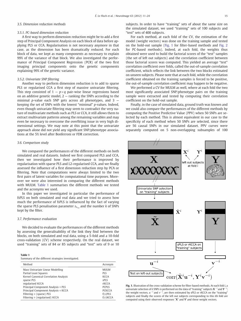
3.7. Performance evaluation

We decided to evaluate the performances of the different methodsby assessing the generalisability of the link they find between theblocks, on both simulated and real data, using a 5-fold and a 10-foldcross-validation (CV) scheme respectively. On the real dataset, weused “training” sets of 84 or 85 subjects and “test” sets of 9 or 10

Table 1Summary of the different strategies investigated.

Method Acronym

Mass Univariate Linear Modelling MULMPartial Least Squares PLSKernel Canonical Correlation Analysis KCCAsparse PLS sPLSregularised KCCA rKCCAPrincipal Component Analysis+PLS PCPLSPrincipal Component Analysis+KCCA PCKCCAFiltering+(sparse) PLS f(s)PLSFiltering+(regularised) KCCA f(r)KCCA

subjects. In order to have “training” sets of about the same size onthe simulated dataset, we used “training” sets of 100 subjects and“test” sets of 400 subjects.

For each method, at each fold of the CV, the estimation of themodel (weight vectors) was done on the training sample and testedon the hold-out sample (Fig. 1 for filter-based methods and Fig. 2for PC-based methods). Indeed, at each fold, the weights thusobtained were used to build the factorial scores of the “test” samples(the set of left out subjects) and the correlation coefficient betweenthose factorial scores was computed. This yielded an average “test”correlation coefficient over folds, called the out-of-sample correlationcoefficient, which reflects the link between the two blocks estimatedon unseen subjects. Please note that at each fold, while the correlationcoefficient obtained on the training samples is forced to be positive,the out-of-sample correlation coefficient may happen to be negative.

We performed a CV for MULM as well, where at each fold the twomost significantly associated SNP/phenotype pairs on the trainingsample were extracted and tested by computing their correlationcoefficient on the hold-out sample.

Finally, in the case of simulated data, ground truth was known andwe could also compare the performances of the different methods bycomputing the Positive Predictive Value (PPV) when 50 SNPs are se-lected by each method. This is almost equivalent in our case to thespecificity of each method when 50 SNPs are selected, since thereare 56 causal SNPs in our simulated dataset. PPV curves wereseparately computed on 5 non-overlapping subsamples of 100

Fig. 1. Illustration of the cross-validation scheme for filter-basedmethods. At each fold i, aunivariate selection of k SNPs is performed on the data of “training” subjects X−i and Y−i;the weight vectors, u−i and v−i, are then estimated by sPLS or rKCCA on the “training”subjects and finally the scores of the left out subjects corresponding to this ith fold arecomputed using their observed responses ˜X i and Yi and these weight vectors.

16 É. Le Floch et al. / NeuroImage 63 (2012) 11–24

observations and averaged over these 5 subsamples. It should benoted that the informative SNPs that are not considered as causalare only slightly correlated to causal SNPs. Therefore they were re-moved to compute the PPV, since they could not really be identifiedas true or false effects.

4. Results

4.1. Performance assessment on simulated data

4.1.1. Influence of regularisationWe were first interested in comparing the performances of PLS

and CCA when the number of SNPs p increases, from 200 (mostlymade of the 198 informative features) up to 85,772 SNPs (mostlymade of noise), and investigating the influence of L1 regularisationon PLS and of L2 regularisation on CCA.

Fig. 3, on the left panel, shows the out-of-sample correlation coef-ficients obtained with the different methods for the two first compo-nent pairs, and it shows that in the lower dimensional space (p=200) mostly made of informative features, the pure CCA, rKCCA with-out regularisation (λ2=0), has overfitted the “training” data on thefirst component pair (“training” corr. ≈1 and “test” corr. ≈0.2).Such a result highlights the limits of pure CCA to deal with situationswhere the number of training samples (100) is smaller than the di-mension (p=200). However, with a suitable regularisation in sucha low-dimensional setting, rKCCA(λ2=100) performed better than

Fig. 2. Illustration of the cross-validation scheme for PC-based methods. At each fold i, twoPCAs are performed on SNPs and on phenotypes of “training” subjects X−i and Y−i; theweight vectors, u−i and v−i, are then estimated by PLS or KCCA on the “training” subjects,and finally the scores of the left out subjects corresponding to this ith fold are computedusing the projection of their observed responses on the principal components, ˜X i and˜Y i , and these weight vectors.

all other methods, notably all (sparse) PLS. These results wereexpected since the evaluation criterion (correlation between factorialscores) is exactly the one which is maximised by CCA.

Nevertheless, the increase of space dimensionality (with irrele-vant features) clearly highlights the superiority of PLS and more nota-bly sPLS over rKCCA in high-dimensional settings: the performance ofrKCCA rapidly decreases while sPLS (sλ1X

=0.1) tolerates an increaseof the dimensionality up to 1000 features before its performancestarts to decrease. One may note that as expected theoretically,along with the increase of penalisation (λ2), rKCCA curves smoothlyconverge toward PLS.

On the second component pair, the results are less clearly inter-pretable. However (s)PLS curves are above the rKCCA ones.

The four graphs on the right panel of Fig. 3 demonstrate the supe-riority of sPLS methods to identify causal SNPs on the two first geneticcomponents. Indeed, for each method and for different values of p, wecomputed the PPV for the two first genetic components and for eachsimulated pattern. PPV curves show a smooth increase of the perfor-mance, when moving from unregularised CCA (rKCCA(λ2=0)) tostrongly regularised PLS (sPLS(sλ1X

=0.1)). Moreover, while theout-of-sample correlation coefficient was not an appropriate measureto distinguish between the two causal patterns, PPV curves werecomputed for each pattern separately. One may note that the PPVon the first genetic component appears to be much higher for thefirst pattern than for the second pattern, especially in low dimen-sions, while the opposite trend is observed on the second geneticcomponent. This observation tends to show that the first causal pat-tern is captured by the first component pair, while the second patternis captured by the second pair. It should be noted that the PPV evenreaches one when p=200 for the first pattern on the first component,meaning that only true positives from the first pattern are detectedon this component. Similarly, the PPV reaches one when p=200 forthe second pattern on the second component.

4.1.2. Influence of the dimension reduction stepThen we investigated the influence of a first step of dimension

reduction. Fig. 4 presents different dimension reduction strategies: Prin-cipal Component (PC), filter (f), sparse (s) and combined filter+sparse(fs)methods. Here the parameter setting, 50 selected SNPs,was derivedfrom the known ground truth (56 true causal SNPs). The 50 SNPs wereeither the 50 best ranked SNPs for (f) methods, the 50 non-null weightsfor sparse PLS or a combination of both: either 10% of the 500 bestranked SNPs or 50% of 100 for fsPLS.

Fig. 4, on the left panel, shows that all PC-based methods (greencurves) failed to identify generalisable covariations when the numberof irrelevant features increases.

Dimension reduction based on filtering slightly improved the per-formance of CCA and greatly improved the performance of PLS:fPLS(k=50) is the second best approach in our comparative study.

Moreover, as previously observed in Fig. 3, L1 regularisation limitsthe overfitting phenomenon (see sPLS(sλ1X

∗p=50) in Fig. 4) and de-lays the decrease of PLS performance when the dimensionality in-creases. Finally the best performance is obtained by combiningfiltering and L1 regularisation: fsPLS(k=100, sλ1X

=0.5), whichkeeps 100 SNPs after filtering and selects 50% of those SNPs by sPLS.Please note that the performance of fsPLS (k=500, sda1X=0.1) islower and similar to that of sPLS(50) in low dimensions, but becomesmore robust than sPLS and equivalent to fsPLS(k=100, sλ1X

=0.5) inhigher dimensions. However, the purely univariate strategy basedon MULM shows poor generalisability, which suggests that eventhough filtering appears necessary to remove irrelevant features, itis not able to capture the imaging/genetics link by itself and needs tobe combined with a multivariate step which will take advantage ofthe cumulative effects of several SNPs. Nevertheless, it should benoted that the way we assessed the generalisability of MULMwas arbi-trary, sincewe only looked at the two best SNP/phenotype associations.

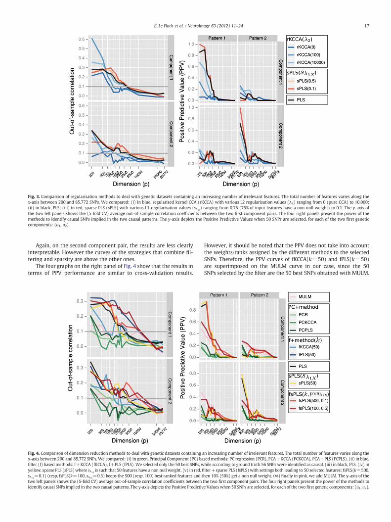
Fig. 3. Comparison of regularisation methods to deal with genetic datasets containing an increasing number of irrelevant features. The total number of features varies along thex-axis between 200 and 85,772 SNPs. We compared: (i) in blue, regularised kernel CCA (rKCCA) with various L2 regularisation values (λ2) ranging from 0 (pure CCA) to 10,000;(ii) in black, PLS; (iii) in red, sparse PLS (sPLS) with various L1 regularisation values (sλ1X

) ranging from 0.75 (75% of input features have a non null weight) to 0.1. The y‐axis ofthe two left panels shows the (5‐fold CV) average out‐of‐sample correlation coefficients between the two first component pairs. The four right panels present the power of themethods to identify causal SNPs implied in the two causal patterns. The y‐axis depicts the Positive Predictive Values when 50 SNPs are selected, for each of the two first geneticcomponents: (u1, u2).

17É. Le Floch et al. / NeuroImage 63 (2012) 11–24

Again, on the second component pair, the results are less clearlyinterpretable. However the curves of the strategies that combine fil-tering and sparsity are above the other ones.

The four graphs on the right panel of Fig. 4 show that the results interms of PPV performance are similar to cross-validation results.

Fig. 4. Comparison of dimension reduction methods to deal with genetic datasets containing ax-axis between 200 and 85,772 SNPs. We compared: (i) in green, Principal Component (PC) bafilter (f) based methods: f+KCCA (fKCCA), f+PLS (fPLS). We selected only the 50 best SNPs, wyellow, sparse PLS (sPLS)where sλ1X

is such that 50 features have a non null weight. (v) in red, fisλ1X

=0.1) (resp. fsPLS(k=100, sλ1X=0.5) keeps the 500 (resp. 100) best ranked features and t

two left panels shows the (5‐fold CV) average out‐of‐sample correlation coefficients betweenidentify causal SNPs implied in the two causal patterns. The y‐axis depicts the Positive Predictiv

However, it should be noted that the PPV does not take into accountthe weights/ranks assigned by the different methods to the selectedSNPs. Therefore, the PPV curves of fKCCA(k=50) and fPLS(k=50)are superimposed on the MULM curve in our case, since the 50SNPs selected by the filter are the 50 best SNPs obtained with MULM.

n increasing number of irrelevant features. The total number of features varies along thesedmethods: PC regression (PCR), PCA+KCCA (PCKCCA), PCA+PLS (PCPLS). (ii) in blue,hile according to ground truth 56 SNPs were identified as causal. (iii) in black, PLS. (iv) inlter+sparse PLS (fsPLS) with settings both leading to 50 selected features: fsPLS(k=500,hen 10% (50%) get a non null weight. (vi) finally in pink, we add MULM. The y‐axis of thethe two first component pairs. The four right panels present the power of the methods toe Valueswhen 50 SNPs are selected, for each of the two first genetic components: (u1, u2).

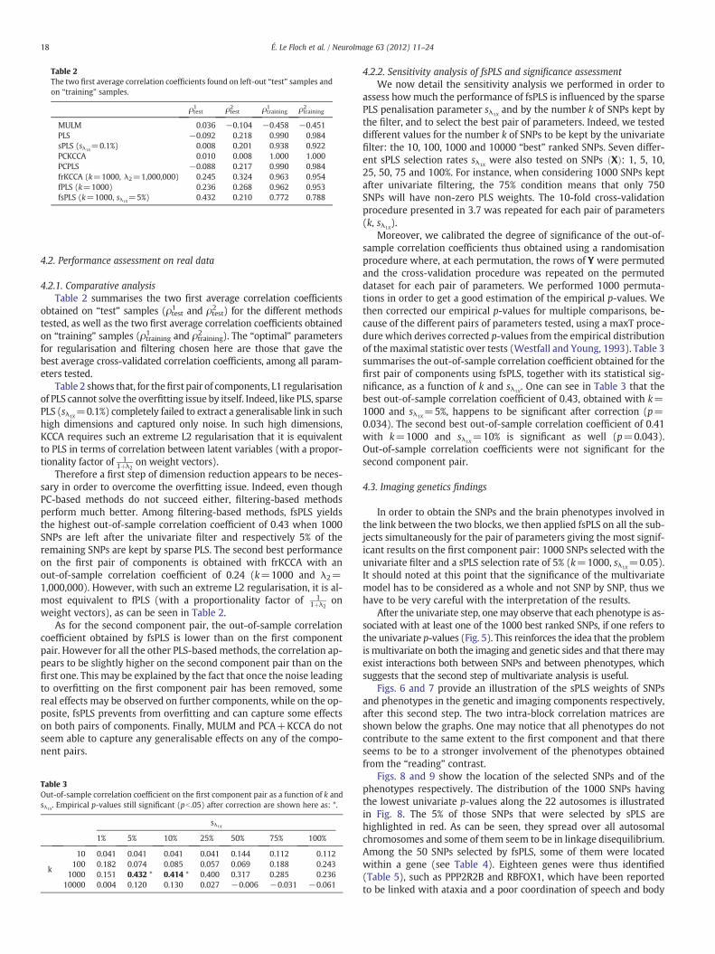
Table 2The two first average correlation coefficients found on left-out “test” samples andon “training” samples.

ρtest1 ρtest2 ρtraining1 ρtraining2

MULM 0.036 −0.104 −0.458 −0.451PLS −0.092 0.218 0.990 0.984sPLS (sλ1X

=0.1%) 0.008 0.201 0.938 0.922PCKCCA 0.010 0.008 1.000 1.000PCPLS −0.088 0.217 0.990 0.984frKCCA (k=1000, λ2=1,000,000) 0.245 0.324 0.963 0.954fPLS (k=1000) 0.236 0.268 0.962 0.953fsPLS (k=1000, sλ1X

=5%) 0.432 0.210 0.772 0.788

18 É. Le Floch et al. / NeuroImage 63 (2012) 11–24

4.2. Performance assessment on real data

4.2.1. Comparative analysisTable 2 summarises the two first average correlation coefficients

obtained on “test” samples (ρtest1 and ρtest2 ) for the different methodstested, as well as the two first average correlation coefficients obtainedon “training” samples (ρtraining1 and ρtraining2 ). The “optimal” parametersfor regularisation and filtering chosen here are those that gave thebest average cross-validated correlation coefficients, among all param-eters tested.

Table 2 shows that, for thefirst pair of components, L1 regularisationof PLS cannot solve the overfitting issue by itself. Indeed, like PLS, sparsePLS (sλ1X

=0.1%) completely failed to extract a generalisable link in suchhigh dimensions and captured only noise. In such high dimensions,KCCA requires such an extreme L2 regularisation that it is equivalentto PLS in terms of correlation between latent variables (with a propor-tionality factor of 1

1þλ2on weight vectors).

Therefore a first step of dimension reduction appears to be neces-sary in order to overcome the overfitting issue. Indeed, even thoughPC-based methods do not succeed either, filtering-based methodsperform much better. Among filtering-based methods, fsPLS yieldsthe highest out-of-sample correlation coefficient of 0.43 when 1000SNPs are left after the univariate filter and respectively 5% of theremaining SNPs are kept by sparse PLS. The second best performanceon the first pair of components is obtained with frKCCA with anout-of-sample correlation coefficient of 0.24 (k=1000 and λ2=1,000,000). However, with such an extreme L2 regularisation, it is al-most equivalent to fPLS (with a proportionality factor of 1

1þλ2on

weight vectors), as can be seen in Table 2.As for the second component pair, the out-of-sample correlation

coefficient obtained by fsPLS is lower than on the first componentpair. However for all the other PLS-based methods, the correlation ap-pears to be slightly higher on the second component pair than on thefirst one. This may be explained by the fact that once the noise leadingto overfitting on the first component pair has been removed, somereal effects may be observed on further components, while on the op-posite, fsPLS prevents from overfitting and can capture some effectson both pairs of components. Finally, MULM and PCA+KCCA do notseem able to capture any generalisable effects on any of the compo-nent pairs.

Table 3Out-of-sample correlation coefficient on the first component pair as a function of k andsλ1X

. Empirical p-values still significant (pb .05) after correction are shown here as: *.

sλ1X

1% 5% 10% 25% 50% 75% 100%

k

10 0.041 0.041 0.041 0.041 0.144 0.112 0.112100 0.182 0.074 0.085 0.057 0.069 0.188 0.243

1000 0.151 0.432 * 0.414 * 0.400 0.317 0.285 0.23610000 0.004 0.120 0.130 0.027 −0.006 −0.031 −0.061

4.2.2. Sensitivity analysis of fsPLS and significance assessmentWe now detail the sensitivity analysis we performed in order to

assess howmuch the performance of fsPLS is influenced by the sparsePLS penalisation parameter sλ1X

and by the number k of SNPs kept bythe filter, and to select the best pair of parameters. Indeed, we testeddifferent values for the number k of SNPs to be kept by the univariatefilter: the 10, 100, 1000 and 10000 “best” ranked SNPs. Seven differ-ent sPLS selection rates sλ1X

were also tested on SNPs Xð Þ: 1, 5, 10,25, 50, 75 and 100%. For instance, when considering 1000 SNPs keptafter univariate filtering, the 75% condition means that only 750SNPs will have non-zero PLS weights. The 10-fold cross-validationprocedure presented in 3.7 was repeated for each pair of parameters(k, sλ1X

).Moreover, we calibrated the degree of significance of the out-of-

sample correlation coefficients thus obtained using a randomisationprocedure where, at each permutation, the rows of Y were permutedand the cross-validation procedure was repeated on the permuteddataset for each pair of parameters. We performed 1000 permuta-tions in order to get a good estimation of the empirical p-values. Wethen corrected our empirical p-values for multiple comparisons, be-cause of the different pairs of parameters tested, using a maxT proce-dure which derives corrected p-values from the empirical distributionof the maximal statistic over tests (Westfall and Young, 1993). Table 3summarises the out-of-sample correlation coefficient obtained for thefirst pair of components using fsPLS, together with its statistical sig-nificance, as a function of k and sλ1X

. One can see in Table 3 that thebest out-of-sample correlation coefficient of 0.43, obtained with k=1000 and sλ1X

=5%, happens to be significant after correction (p=0.034). The second best out-of-sample correlation coefficient of 0.41with k=1000 and sλ1X

=10% is significant as well (p=0.043).Out-of-sample correlation coefficients were not significant for thesecond component pair.

4.3. Imaging genetics findings

In order to obtain the SNPs and the brain phenotypes involved inthe link between the two blocks, we then applied fsPLS on all the sub-jects simultaneously for the pair of parameters giving the most signif-icant results on the first component pair: 1000 SNPs selected with theunivariate filter and a sPLS selection rate of 5% (k=1000, sλ1X

=0.05).It should noted at this point that the significance of the multivariatemodel has to be considered as a whole and not SNP by SNP, thus wehave to be very careful with the interpretation of the results.

After the univariate step, onemay observe that each phenotype is as-sociated with at least one of the 1000 best ranked SNPs, if one refers tothe univariate p-values (Fig. 5). This reinforces the idea that the problemismultivariate on both the imaging and genetic sides and that theremayexist interactions both between SNPs and between phenotypes, whichsuggests that the second step of multivariate analysis is useful.

Figs. 6 and 7 provide an illustration of the sPLS weights of SNPsand phenotypes in the genetic and imaging components respectively,after this second step. The two intra-block correlation matrices areshown below the graphs. One may notice that all phenotypes do notcontribute to the same extent to the first component and that thereseems to be to a stronger involvement of the phenotypes obtainedfrom the “reading” contrast.

Figs. 8 and 9 show the location of the selected SNPs and of thephenotypes respectively. The distribution of the 1000 SNPs havingthe lowest univariate p-values along the 22 autosomes is illustratedin Fig. 8. The 5% of those SNPs that were selected by sPLS arehighlighted in red. As can be seen, they spread over all autosomalchromosomes and some of them seem to be in linkage disequilibrium.Among the 50 SNPs selected by fsPLS, some of them were locatedwithin a gene (see Table 4). Eighteen genes were thus identified(Table 5), such as PPP2R2B and RBFOX1, which have been reportedto be linked with ataxia and a poor coordination of speech and body

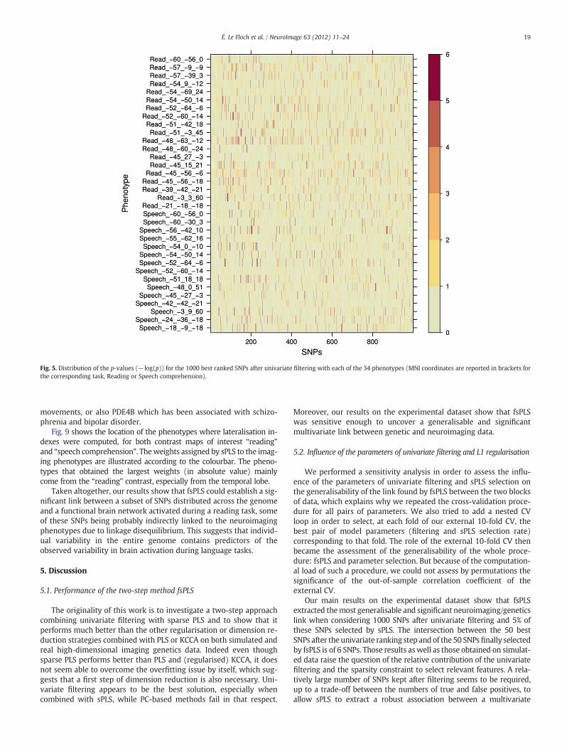
Fig. 5. Distribution of the p-values (− log(p)) for the 1000 best ranked SNPs after univariate filtering with each of the 34 phenotypes (MNI coordinates are reported in brackets forthe corresponding task, Reading or Speech comprehension).

19É. Le Floch et al. / NeuroImage 63 (2012) 11–24

movements, or also PDE4B which has been associated with schizo-phrenia and bipolar disorder.

Fig. 9 shows the location of the phenotypes where lateralisation in-dexes were computed, for both contrast maps of interest “reading”and “speech comprehension”. Theweights assigned by sPLS to the imag-ing phenotypes are illustrated according to the colourbar. The pheno-types that obtained the largest weights (in absolute value) mainlycome from the “reading” contrast, especially from the temporal lobe.

Taken altogether, our results show that fsPLS could establish a sig-nificant link between a subset of SNPs distributed across the genomeand a functional brain network activated during a reading task, someof these SNPs being probably indirectly linked to the neuroimagingphenotypes due to linkage disequilibrium. This suggests that individ-ual variability in the entire genome contains predictors of theobserved variability in brain activation during language tasks.

5. Discussion

5.1. Performance of the two-step method fsPLS

The originality of this work is to investigate a two-step approachcombining univariate filtering with sparse PLS and to show that itperforms much better than the other regularisation or dimension re-duction strategies combined with PLS or KCCA on both simulated andreal high-dimensional imaging genetics data. Indeed even thoughsparse PLS performs better than PLS and (regularised) KCCA, it doesnot seem able to overcome the overfitting issue by itself, which sug-gests that a first step of dimension reduction is also necessary. Uni-variate filtering appears to be the best solution, especially whencombined with sPLS, while PC-based methods fail in that respect.

Moreover, our results on the experimental dataset show that fsPLSwas sensitive enough to uncover a generalisable and significantmultivariate link between genetic and neuroimaging data.

5.2. Influence of the parameters of univariate filtering and L1 regularisation

We performed a sensitivity analysis in order to assess the influ-ence of the parameters of univariate filtering and sPLS selection onthe generalisability of the link found by fsPLS between the two blocksof data, which explains why we repeated the cross-validation proce-dure for all pairs of parameters. We also tried to add a nested CVloop in order to select, at each fold of our external 10-fold CV, thebest pair of model parameters (filtering and sPLS selection rate)corresponding to that fold. The role of the external 10-fold CV thenbecame the assessment of the generalisability of the whole proce-dure: fsPLS and parameter selection. But because of the computation-al load of such a procedure, we could not assess by permutations thesignificance of the out-of-sample correlation coefficient of theexternal CV.

Our main results on the experimental dataset show that fsPLSextracted themost generalisable and significant neuroimaging/geneticslink when considering 1000 SNPs after univariate filtering and 5% ofthese SNPs selected by sPLS. The intersection between the 50 bestSNPs after the univariate ranking step and of the 50 SNPsfinally selectedby fsPLS is of 6 SNPs. Those results as well as those obtained on simulat-ed data raise the question of the relative contribution of the univariatefiltering and the sparsity constraint to select relevant features. A rela-tively large number of SNPs kept after filtering seems to be required,up to a trade-off between the numbers of true and false positives, toallow sPLS to extract a robust association between a multivariate

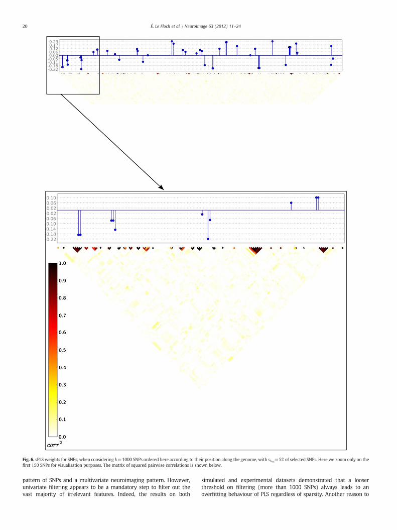
Fig. 6. sPLS weights for SNPs, when considering k=1000 SNPs ordered here according to their position along the genome, with sλ1X=5% of selected SNPs. Here we zoom only on the

first 150 SNPs for visualisation purposes. The matrix of squared pairwise correlations is shown below.

20 É. Le Floch et al. / NeuroImage 63 (2012) 11–24

pattern of SNPs and a multivariate neuroimaging pattern. However,univariate filtering appears to be a mandatory step to filter out thevast majority of irrelevant features. Indeed, the results on both

simulated and experimental datasets demonstrated that a looserthreshold on filtering (more than 1000 SNPs) always leads to anoverfitting behaviour of PLS regardless of sparsity. Another reason to

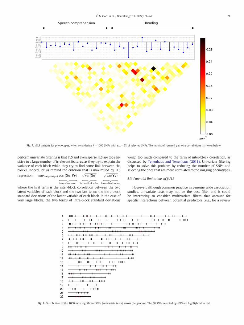
Fig. 7. sPLS weights for phenotypes, when considering k=1000 SNPs with sλ1X=5% of selected SNPs. The matrix of squared pairwise correlations is shown below.

21É. Le Floch et al. / NeuroImage 63 (2012) 11–24

perform univariate filtering is that PLS and even sparse PLS are too sen-sitive to a large number of irrelevant features, as they try to explain thevariance of each block while they try to find some link between theblocks. Indeed, let us remind the criterion that is maximised by PLS

regression: max∥u∥2¼∥v∥2¼1 corr Xu;Yvð Þ|fflfflfflfflfflfflfflfflfflffl{zfflfflfflfflfflfflfflfflfflffl}Inter−block corr

ffiffiffiffiffiffiffiffiffiffiffiffiffiffiffiffiffivar Xuð Þ

p|fflfflfflfflfflfflffl{zfflfflfflfflfflfflffl}

Intra−block stdev

ffiffiffiffiffiffiffiffiffiffiffiffiffiffiffiffiffivar Yvð Þ

p|fflfflfflfflfflfflffl{zfflfflfflfflfflfflffl}

Intra−block stdev

,

where the first term is the inter-block correlation between the twolatent variables of each block and the two last terms the intra-blockstandard deviations of the latent variable of each block. In the case ofvery large blocks, the two terms of intra-block standard deviations

Fig. 8. Distribution of the 1000 most significant SNPs (univariate tests) acr

weigh too much compared to the term of inter-block correlation, asdiscussed by Tenenhaus and Tenenhaus (2011). Univariate filteringhelps to solve this problem by reducing the number of SNPs andselecting the ones that are more correlated to the imaging phenotypes.

5.3. Potential limitations of fsPLS

However, although common practice in genome wide associationstudies, univariate tests may not be the best filter and it couldbe interesting to consider multivariate filters that account forspecific interactions between potential predictors (e.g., for a review

oss the genome. The 50 SNPs selected by sPLS are highlighted in red.

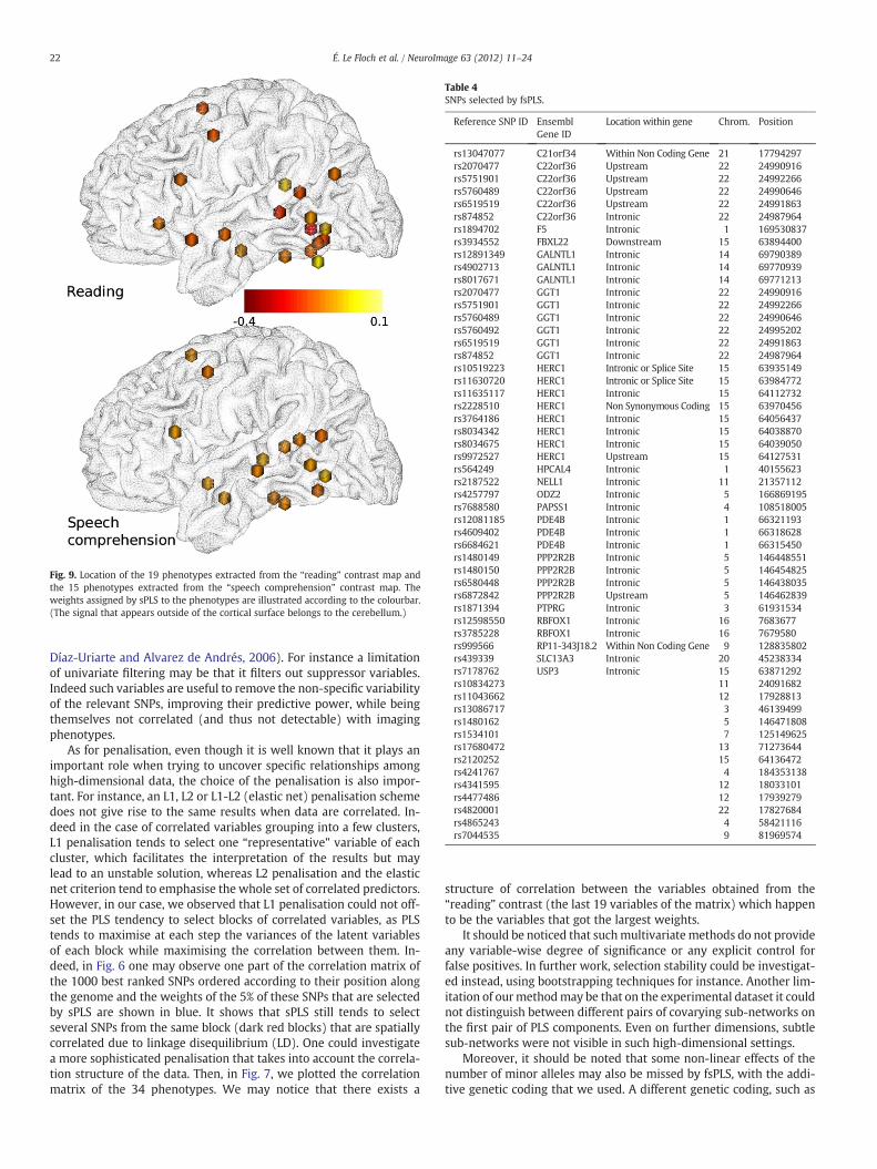
Fig. 9. Location of the 19 phenotypes extracted from the “reading” contrast map andthe 15 phenotypes extracted from the “speech comprehension” contrast map. Theweights assigned by sPLS to the phenotypes are illustrated according to the colourbar.(The signal that appears outside of the cortical surface belongs to the cerebellum.)

Table 4SNPs selected by fsPLS.

Reference SNP ID EnsemblGene ID

Location within gene Chrom. Position

rs13047077 C21orf34 Within Non Coding Gene 21 17794297rs2070477 C22orf36 Upstream 22 24990916rs5751901 C22orf36 Upstream 22 24992266rs5760489 C22orf36 Upstream 22 24990646rs6519519 C22orf36 Upstream 22 24991863rs874852 C22orf36 Intronic 22 24987964rs1894702 F5 Intronic 1 169530837rs3934552 FBXL22 Downstream 15 63894400rs12891349 GALNTL1 Intronic 14 69790389rs4902713 GALNTL1 Intronic 14 69770939rs8017671 GALNTL1 Intronic 14 69771213rs2070477 GGT1 Intronic 22 24990916rs5751901 GGT1 Intronic 22 24992266rs5760489 GGT1 Intronic 22 24990646rs5760492 GGT1 Intronic 22 24995202rs6519519 GGT1 Intronic 22 24991863rs874852 GGT1 Intronic 22 24987964rs10519223 HERC1 Intronic or Splice Site 15 63935149rs11630720 HERC1 Intronic or Splice Site 15 63984772rs11635117 HERC1 Intronic 15 64112732rs2228510 HERC1 Non Synonymous Coding 15 63970456rs3764186 HERC1 Intronic 15 64056437rs8034342 HERC1 Intronic 15 64038870rs8034675 HERC1 Intronic 15 64039050rs9972527 HERC1 Upstream 15 64127531rs564249 HPCAL4 Intronic 1 40155623rs2187522 NELL1 Intronic 11 21357112rs4257797 ODZ2 Intronic 5 166869195rs7688580 PAPSS1 Intronic 4 108518005rs12081185 PDE4B Intronic 1 66321193rs4609402 PDE4B Intronic 1 66318628rs6684621 PDE4B Intronic 1 66315450rs1480149 PPP2R2B Intronic 5 146448551rs1480150 PPP2R2B Intronic 5 146454825rs6580448 PPP2R2B Intronic 5 146438035rs6872842 PPP2R2B Upstream 5 146462839rs1871394 PTPRG Intronic 3 61931534rs12598550 RBFOX1 Intronic 16 7683677rs3785228 RBFOX1 Intronic 16 7679580rs999566 RP11-343J18.2 Within Non Coding Gene 9 128835802rs439339 SLC13A3 Intronic 20 45238334rs7178762 USP3 Intronic 15 63871292rs10834273 11 24091682rs11043662 12 17928813rs13086717 3 46139499rs1480162 5 146471808rs1534101 7 125149625rs17680472 13 71273644rs2120252 15 64136472rs4241767 4 184353138rs4341595 12 18033101rs4477486 12 17939279rs4820001 22 17827684rs4865243 4 58421116rs7044535 9 81969574

22 É. Le Floch et al. / NeuroImage 63 (2012) 11–24

Díaz-Uriarte and Alvarez de Andrés, 2006). For instance a limitationof univariate filtering may be that it filters out suppressor variables.Indeed such variables are useful to remove the non-specific variabilityof the relevant SNPs, improving their predictive power, while beingthemselves not correlated (and thus not detectable) with imagingphenotypes.

As for penalisation, even though it is well known that it plays animportant role when trying to uncover specific relationships amonghigh-dimensional data, the choice of the penalisation is also impor-tant. For instance, an L1, L2 or L1-L2 (elastic net) penalisation schemedoes not give rise to the same results when data are correlated. In-deed in the case of correlated variables grouping into a few clusters,L1 penalisation tends to select one “representative” variable of eachcluster, which facilitates the interpretation of the results but maylead to an unstable solution, whereas L2 penalisation and the elasticnet criterion tend to emphasise the whole set of correlated predictors.However, in our case, we observed that L1 penalisation could not off-set the PLS tendency to select blocks of correlated variables, as PLStends to maximise at each step the variances of the latent variablesof each block while maximising the correlation between them. In-deed, in Fig. 6 one may observe one part of the correlation matrix ofthe 1000 best ranked SNPs ordered according to their position alongthe genome and the weights of the 5% of these SNPs that are selectedby sPLS are shown in blue. It shows that sPLS still tends to selectseveral SNPs from the same block (dark red blocks) that are spatiallycorrelated due to linkage disequilibrium (LD). One could investigatea more sophisticated penalisation that takes into account the correla-tion structure of the data. Then, in Fig. 7, we plotted the correlationmatrix of the 34 phenotypes. We may notice that there exists a

structure of correlation between the variables obtained from the“reading” contrast (the last 19 variables of the matrix) which happento be the variables that got the largest weights.

It should be noticed that suchmultivariate methods do not provideany variable-wise degree of significance or any explicit control forfalse positives. In further work, selection stability could be investigat-ed instead, using bootstrapping techniques for instance. Another lim-itation of ourmethodmay be that on the experimental dataset it couldnot distinguish between different pairs of covarying sub-networks onthe first pair of PLS components. Even on further dimensions, subtlesub-networks were not visible in such high-dimensional settings.

Moreover, it should be noted that some non-linear effects of thenumber of minor alleles may also be missed by fsPLS, with the addi-tive genetic coding that we used. A different genetic coding, such as

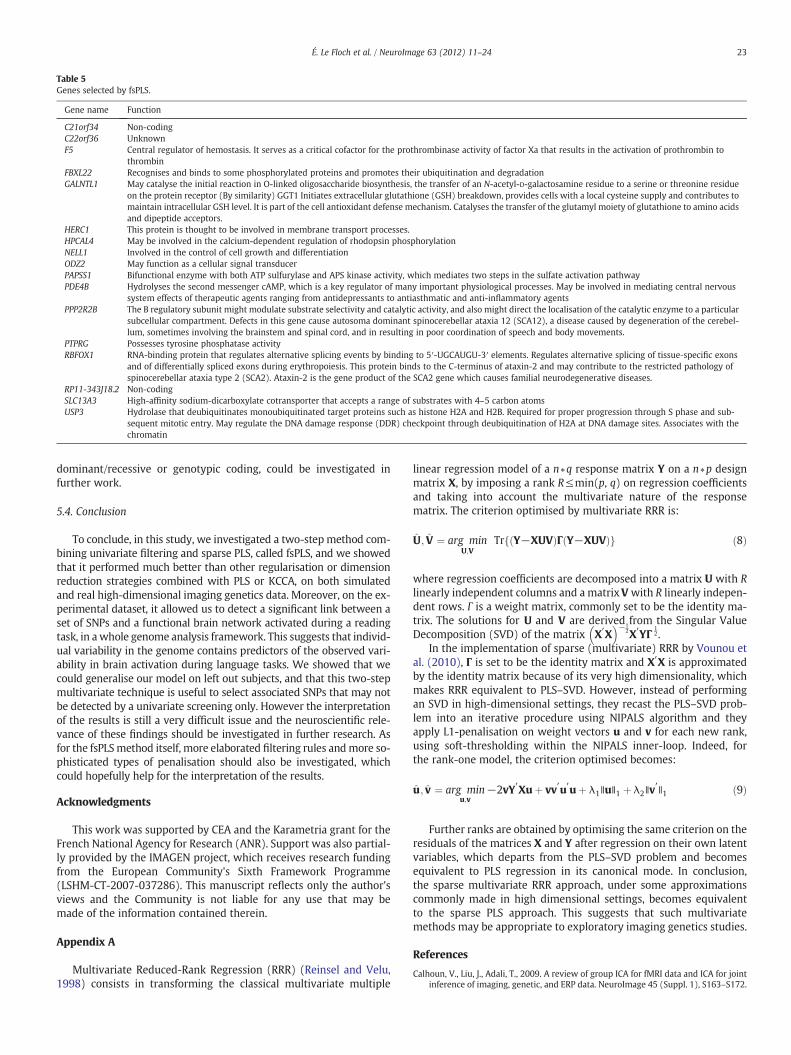
Table 5Genes selected by fsPLS.

Gene name Function

C21orf34 Non-codingC22orf36 UnknownF5 Central regulator of hemostasis. It serves as a critical cofactor for the prothrombinase activity of factor Xa that results in the activation of prothrombin to

thrombinFBXL22 Recognises and binds to some phosphorylated proteins and promotes their ubiquitination and degradationGALNTL1 May catalyse the initial reaction in O-linked oligosaccharide biosynthesis, the transfer of an N-acetyl-D-galactosamine residue to a serine or threonine residue

on the protein receptor (By similarity) GGT1 Initiates extracellular glutathione (GSH) breakdown, provides cells with a local cysteine supply and contributes tomaintain intracellular GSH level. It is part of the cell antioxidant defense mechanism. Catalyses the transfer of the glutamyl moiety of glutathione to amino acidsand dipeptide acceptors.

HERC1 This protein is thought to be involved in membrane transport processes.HPCAL4 May be involved in the calcium-dependent regulation of rhodopsin phosphorylationNELL1 Involved in the control of cell growth and differentiationODZ2 May function as a cellular signal transducerPAPSS1 Bifunctional enzyme with both ATP sulfurylase and APS kinase activity, which mediates two steps in the sulfate activation pathwayPDE4B Hydrolyses the second messenger cAMP, which is a key regulator of many important physiological processes. May be involved in mediating central nervous

system effects of therapeutic agents ranging from antidepressants to antiasthmatic and anti-inflammatory agentsPPP2R2B The B regulatory subunit might modulate substrate selectivity and catalytic activity, and also might direct the localisation of the catalytic enzyme to a particular

subcellular compartment. Defects in this gene cause autosoma dominant spinocerebellar ataxia 12 (SCA12), a disease caused by degeneration of the cerebel-lum, sometimes involving the brainstem and spinal cord, and in resulting in poor coordination of speech and body movements.

PTPRG Possesses tyrosine phosphatase activityRBFOX1 RNA-binding protein that regulates alternative splicing events by binding to 5′-UGCAUGU-3′ elements. Regulates alternative splicing of tissue‐specific exons

and of differentially spliced exons during erythropoiesis. This protein binds to the C-terminus of ataxin-2 and may contribute to the restricted pathology ofspinocerebellar ataxia type 2 (SCA2). Ataxin-2 is the gene product of the SCA2 gene which causes familial neurodegenerative diseases.

RP11-343J18.2 Non-codingSLC13A3 High-affinity sodium-dicarboxylate cotransporter that accepts a range of substrates with 4–5 carbon atomsUSP3 Hydrolase that deubiquitinates monoubiquitinated target proteins such as histone H2A and H2B. Required for proper progression through S phase and sub-

sequent mitotic entry. May regulate the DNA damage response (DDR) checkpoint through deubiquitination of H2A at DNA damage sites. Associates with thechromatin

23É. Le Floch et al. / NeuroImage 63 (2012) 11–24

dominant/recessive or genotypic coding, could be investigated infurther work.

5.4. Conclusion

To conclude, in this study, we investigated a two-step method com-bining univariate filtering and sparse PLS, called fsPLS, and we showedthat it performed much better than other regularisation or dimensionreduction strategies combined with PLS or KCCA, on both simulatedand real high-dimensional imaging genetics data. Moreover, on the ex-perimental dataset, it allowed us to detect a significant link between aset of SNPs and a functional brain network activated during a readingtask, in awhole genome analysis framework. This suggests that individ-ual variability in the genome contains predictors of the observed vari-ability in brain activation during language tasks. We showed that wecould generalise our model on left out subjects, and that this two-stepmultivariate technique is useful to select associated SNPs that may notbe detected by a univariate screening only. However the interpretationof the results is still a very difficult issue and the neuroscientific rele-vance of these findings should be investigated in further research. Asfor the fsPLSmethod itself, more elaborated filtering rules andmore so-phisticated types of penalisation should also be investigated, whichcould hopefully help for the interpretation of the results.

Acknowledgments

This work was supported by CEA and the Karametria grant for theFrench National Agency for Research (ANR). Support was also partial-ly provided by the IMAGEN project, which receives research fundingfrom the European Community's Sixth Framework Programme(LSHM-CT-2007-037286). This manuscript reflects only the author'sviews and the Community is not liable for any use that may bemade of the information contained therein.

Appendix A

Multivariate Reduced-Rank Regression (RRR) (Reinsel and Velu,1998) consists in transforming the classical multivariate multiple

linear regression model of a n∗q response matrix Y on a n∗p designmatrix X, by imposing a rank R≤min(p, q) on regression coefficientsand taking into account the multivariate nature of the responsematrix. The criterion optimised by multivariate RRR is:

U; V ¼ arg minU;V

Tr Y−XUVð ÞΓ Y−XUVð Þf g ð8Þ

where regression coefficients are decomposed into a matrix U with Rlinearly independent columns and a matrixV with R linearly indepen-dent rows. Γ is a weight matrix, commonly set to be the identity ma-trix. The solutions for U and V are derived from the Singular ValueDecomposition (SVD) of the matrix X′X

� �−12X′YΓ

12.

In the implementation of sparse (multivariate) RRR by Vounou etal. (2010), Γ is set to be the identity matrix and X′X is approximatedby the identity matrix because of its very high dimensionality, whichmakes RRR equivalent to PLS–SVD. However, instead of performingan SVD in high-dimensional settings, they recast the PLS–SVD prob-lem into an iterative procedure using NIPALS algorithm and theyapply L1-penalisation on weight vectors u and v for each new rank,using soft-thresholding within the NIPALS inner-loop. Indeed, forthe rank-one model, the criterion optimised becomes:

u; v ¼ arg minu;v

−2vY′Xuþ vv′u′uþ λ1∥u∥1 þ λ2∥v′∥1 ð9Þ

Further ranks are obtained by optimising the same criterion on theresiduals of the matrices X and Y after regression on their own latentvariables, which departs from the PLS–SVD problem and becomesequivalent to PLS regression in its canonical mode. In conclusion,the sparse multivariate RRR approach, under some approximationscommonly made in high dimensional settings, becomes equivalentto the sparse PLS approach. This suggests that such multivariatemethods may be appropriate to exploratory imaging genetics studies.

References

Calhoun, V., Liu, J., Adali, T., 2009. A review of group ICA for fMRI data and ICA for jointinference of imaging, genetic, and ERP data. NeuroImage 45 (Suppl. 1), S163–S172.

24 É. Le Floch et al. / NeuroImage 63 (2012) 11–24

Chun, H., Keleş, S., 2010. Sparse partial least squares regression for simultaneousdimension reduction and variable selection. J. R. Stat. Soc. B 72 (1), 3–25.

Clayton, D., Cheung, H.-T., 2007. An R package for analysis of whole-genome associa-tion studies. Hum. Hered. 64, 45–51.

de Bakker, P., Yelensky, R., Peer, I., Gabriel, S., Daly, M., Altshuler, D., 2005. Efficiencyand power in genetic association studies. Nat. Genet. 37 (11), 1217–1223.

Díaz-Uriarte, R., Alvarez de Andrés, S., 2006. Gene selection and classification of micro-array data using random forest. BMC Bioinforma. 7 (3).

Furlanello, C., Serafini, M., Merler, S., Jurman, G., 2003. An accelerated procedure forrecursive feature ranking on microarray data. Neural Netw. 16, 641–648.

Glahn, D.C., Thompson, P.M., Blangero, J., 2007. Neuroimaging endophenotypes: strat-egies for finding genes influencing brain structure and function. Hum. Brain Mapp.28, 488–501.

Feature Extraction: Foundations and Applications. In: Guyon, I., Gunn, S., Nikravesh, M.,Zadeh, L.A. (Eds.), Springer-Verlag.

Hibar, D., Stein, J., Kohannim, O., Jahanshad, N., Saykin, A., Shen, L., Kim, S., Pankratz, N.,Foroud, T., Huentelman, M., Potkin, S., Jack Jr., C., Weiner, M., Toga, A., Thompson,P., the Alzheimer's Disease Neuroimaging Initiative, 2011. Voxelwise gene-wideassociation study (vgenewas): multivariate gene-based association testing in 731elderly subjects. NeuroImage 56, 1875–1891.

Hotelling, H., 1936. Relations between two sets of variates. Biometrika 28, 321–377.Lê Cao, K.-A., Rossouw, D., Robert-Granié, C., Besse, P., 2008. A sparse PLS for variable

selection when integrating omics data. Stat. Appl. Genet. Mol. Biol. 7 (1).Lê Cao, K.-A., Martin, P.G., Robert-Granié, C., Besse, P., 2009. Sparse canonical methods

for biological data integration: application to a cross-platform study. BMCBioinforma. 10 (34).

Li, J., Chen, Y., 2008. Generating samples for association studies based on hapmap data.BMC Bioinforma. 9 (44).

McAllister, T.W., Flashman, L.A., McDonald, B.C., Saykin, A.J., 2006. Mechanisms of cog-nitive dysfunction after mild and moderate TBI (MTBI): evidence from functionalMRI and neurogenetics. J. Neurotrauma 23 (10), 1450–1467.

McIntosh, A., Bookstein, F., Haxby, J., Grady, C., 1996. Spatial pattern analysis of func-tional brain images using partial least squares. NeuroImage 3, 143–157.

Parkhomenko, E., Tritchler, D., Beyene, J., 2007. Genome-wide sparse canonical correla-tion of gene expression with genotypes. BMC Proc. 1 (Suppl. 1), S119.

Parkhomenko, E., Tritchler, D., Beyene, J., 2009. Sparse canonical correlation analysiswith application to genomic data integration. Stat. Appl. Genet. Mol. Biol. 8 (1)Article 1.

Paulesu, E., Demonet, J.-F., Fazio, F., McCrory, E., Chanoine, V., Brunswick, N., Cappa, F.,Cossu, G., Habib, M., Frith, C., Frith, U., 2001. Dyslexia: cultural diversity andbiological unity. Science 291, 2165–2167.

Pinel, P., Dehaene, S., 2009. Beyond hemispheric dominance: brain regions underlying thejoint lateralization of language and arithmetic to the left hemisphere. J. Cogn. Neurosci.http://dx.doi.org/10.1162/jocn.2009.21184 Posted Online January 13, 2009.

Pinel, P., Thirion, B., Meriaux, S., Jobert, A., Serres, J., Le Bihan, D., Poline, J.-B., Dehaene,S., 2007. Fast reproducible identification and large-scale databasing of individualfunctional cognitive networks. BMC Neurosci. 8 (91).

R Development Core Team, 2009. R: A language and environment for statisticalcomputing. http://www.R-project.org.

Reinsel, G., Velu, R., 1998. Multivariate Reduced-Rank Regression, Theory and Applica-tions. Springer, New York.

Roffman, J.L., Weiss, A.P., Goff, D.C., Rauch, S.L., Weinberger, D.R., 2006. Neuroimaging-genetic paradigms: a new approach to investigate the pathophysiology and treat-ment of cognitive deficits in schizophrenia. Harv. Rev. Psychiatry 14 (2), 78–91.

Sanna, S., Jackson, A., Nagaraja, R., Willer, C., Chen, W., Bonnycastle, L., Shen, H.,Timpson, N., Lettre, G., Usala, G., Chines, P., Stringham, H., Scott, L., Dei, M., Lai, S.,Albai, G., Crisponi, L., Naitza, S., Doheny, K., Pugh, E., Ben-Shlomo, Y., Ebrahim, S.,Lawlor, D., Bergman, R., Watanabe, R., Uda, M., Tuomilehto, J., Coresh, J.,Hirschhorn, J., Shuldiner, A., Schlessinger, D., Collins, F., Davey Smith, G.,Boerwinkle, E., Cao, A., Boehnke, M., Abecasis, G., Mohlke, K., 2008. Common vari-ants in the GDF5-UQCC region are associated with variation in human height. Nat.Genet. 40, 198–203.

Soneson, C., Lilljebjörn, H., Fioretos, T., Fontes, M., 2010. Integrative analysis of gene ex-pression and copy number alterations using canonical correlation analysis. BMCBioinforma. 11 (191).

Stein, J., Hua, X., Lee, S., Ho, A., Leow, A., Toga, A., Saykin, A., Shen, L., Foroud, T.,Pankratz, N., Huentelman, M., Craig, D., Gerber, J., Allen, A., Corneveaux, J.,DeChairo, B., Potkin, S., Weiner, M., Thompson, P., 2010. Voxelwise genome-wideassociation study (vGWAS). NeuroImage 53, 1160–1174.

Tenenhaus, A., Tenenhaus, M., 2011. Regularized generalized canonical correlationanalysis. Psychometrika 76 (2), 257–284.

Tibshirani, R., 1996. Regression shrinkage and selection via the lasso. J. R. Stat. Soc. B 58(1), 267–288.

Tucker, L., 1958. An inter-battery method of factor analysis. Psychometrika 23 (2),111–136.

Vounou, M., Nichols, T., Montana, G., 2010. Discovering genetic associations with high-dimensional neuroimaging phenotypes: a sparse reduced-rank approach. NeuroImage53, 1147–1159.

Waaijenborg, S., Verselewel de Witt Hamer, P., Zwinderman, A., 2008. Quantifying theassociation between gene expressions and DNA-markers by penalized canonicalcorrelation analysis. Stat. Appl. Genet. Mol. Biol. 7 (1) (Article 3).

Westfall, P., Young, S. (Eds.), 1993. Resampling-Based Multiple Testing. Wiley, NewYork.

Willer, C., Sanna, S., Jackson, A., Scuteri, A., Bonnycastle, L., Clarke, R., Heath, S., Timpson,N., Najjar, S., Stringham, H., Strait, J., Duren, W., Maschio, A., Busonero, F., Mulas, A.,Albai, G., Swift, A., Morken, M., Narisu, N., Bennett, D., Parish, S., Shen, H., Galan, P.,Meneton, P., Hercberg, S., Zelenika, D., Chen, W., Li, Y., Scott, L., Scheet, P., Sundvall,J., Watanabe, R., Nagaraja, R., Ebrahim, S., Lawlor, D., Ben-Shlomo, Y., Davey-Smith,G., Shuldiner, A., Collins, R., Bergman, R., Uda, M., Tuomilehto, J., Cao, A., Collins, F.,Lakatta, E., Lathrop, G., Boehnke, M., Schlessinger, D., Mohlke, K., Abecasis, G.R.,2008. Newly identified loci that influence lipid concentrations and risk of coronaryartery disease. Nat. Genet. 40, 161–169.

Witten, D., Tibshirani, R., 2009. Extensions of sparse canonical correlation analysis,with applications to genomic data. Stat. Appl. Genet. Mol. Biol. 8 (1) (Article 28).

Wold, H., 1966. Multivariate Analysis. Estimation of Principal Components and RelatedModels by Iterative Least Squares. Academic Press, New York, Ch, pp. 391–420.

Wold, S., Martens, H., Wold, H., 1983. The multivariate calibration problem inchemistry solved by the PLS method. In: Ruhe, A., Kastrøm, B. (Eds.), ProceedingsConference Matrix Pencils. : Vol. Lecture Notes in Mathematics. Springer-Verlag,pp. 286–293.

Zou, H., Hastie, T., Tibshirani, R., 2006. Sparse principal component analysis. J. Comput.Graph. Stat. 15 (2), 265–286.