Signs of Susy

Chris Wymant

A thesis presented for the degree of Doctor of Philosophy,2013

Institute for Particle Physics PhenomenologyDepartment of PhysicsUniversity of Durham

UK

1

arX

iv:1

306.

3117

v1 [

hep-

ph]

13

Jun

2013

For my father, for giving me a map but not directions.

2

Abstract

After a brief introduction to 21st century fundamental physics suit-able for the layman with a reasonable level of mathematical competence,I introduce the concept of unnaturalness in Standard Model electroweaksymmetry breaking and Supersymmetry (Susy) as a potential solution.The optimally natural situation in Susy in light of the 2012 discovery ofa Higgs boson is derived, namely that of almost maximal mixing, withthe scalar top partners almost as light as can be. The discovery is alsointerpreted numerically in terms of the Next-to-Minimal Supersymmet-ric Standard Model, with greater emphasis placed on the visibility of theHiggs boson at the observed mass, i.e. on signal strengths. I introducesimple models of gauge-mediated Susy breaking (GMSB), and how theirgeneralisation leads to a richer parameter space. I then investigate therole played by the mediation scale of GMSB: this is found to be as acontrol of the extent to which Yukawa couplings de-tune flavour-blindrelations set by gauge couplings. Finally, issues relating to the discov-ery or exclusion of Susy at colliders are discussed. Bounds are derivedfor the masses of new particles from Large Hadron Collider searches forexcesses of jets and missing energy without leptons, and compared toconstraints arising from Higgs boson searches, for models of GMSB andthe Constrained Minimal Supersymmetric Standard Model. I presenta novel search strategy for new physics signatures with two neutral,stable particles, when such particles are produced by boosted decays.(Susy examples include models with light gravitinos, pseudo-goldstinos,singlinos or new photinos.) The method is shown to produce sharp masspeaks that enhance the visibility of the signal.

3

Contents

I Prelude: From Classical Mechanics To QuantumField Theory 13

0.1 Classical Mechanics . . . . . . . . . . . . . . . . . . . . . . . . . 13

0.2 Special Relativity . . . . . . . . . . . . . . . . . . . . . . . . . . 14

0.3 Quantum Mechanics . . . . . . . . . . . . . . . . . . . . . . . . 16

0.4 Quantum Field Theory . . . . . . . . . . . . . . . . . . . . . . . 18

II Weak-Scale Susy’s Raison d’Etre: The Higgs 22

1 Introduction 22

1.1 Motivation . . . . . . . . . . . . . . . . . . . . . . . . . . . . . . 22

1.2 The Superpotential . . . . . . . . . . . . . . . . . . . . . . . . . 27

1.3 The MSSM . . . . . . . . . . . . . . . . . . . . . . . . . . . . . 28

1.4 Naturalness Under Pressure . . . . . . . . . . . . . . . . . . . . 31

2 Optimal Naturalness 34

2.1 Leading-Order Analysis . . . . . . . . . . . . . . . . . . . . . . . 34

2.2 Higher-Order Effects . . . . . . . . . . . . . . . . . . . . . . . . 37

2.3 Working Backwards – Finding The Stop Mass? . . . . . . . . . . 39

2.4 Implications . . . . . . . . . . . . . . . . . . . . . . . . . . . . . 42

3 The Higgs In The NMSSM 44

3.1 Introducing The NMSSM . . . . . . . . . . . . . . . . . . . . . . 44

3.2 Scanning Parameter Space . . . . . . . . . . . . . . . . . . . . . 45

3.3 Higgs Signals For mχ01< 15 GeV . . . . . . . . . . . . . . . . . . 49

3.4 Higgs Signals For Arbitrary mχ01

. . . . . . . . . . . . . . . . . . 53

III Gauge-Mediated Susy Breaking 56

4 Introduction 56

4.1 R Symmetry And Susy Breaking . . . . . . . . . . . . . . . . . 56

4.2 The Gauge Mediation Parameter Space . . . . . . . . . . . . . . 58

5 The Role Of The Messenger Scale, Sum Rules And RG Invari-ants 63

IV Susy Searches At The LHC 68

4

6 Introduction 706.1 How To (Not) See Susy . . . . . . . . . . . . . . . . . . . . . . . 706.2 Complications At NLO . . . . . . . . . . . . . . . . . . . . . . . 716.3 The Importance Of The LSP . . . . . . . . . . . . . . . . . . . . 73

7 A Historical Detour: Comparing Early LHC Direct SearchesTo LEP Higgs Bounds 757.1 Introduction And Main Results . . . . . . . . . . . . . . . . . . 757.2 Derivation Of The Exclusion Contours . . . . . . . . . . . . . . 767.3 Interpretation Of The Exclusion Contours . . . . . . . . . . . . 80

8 Making The Most Of MET: Mass Reconstruction From Colli-mated Decays 848.1 Introduction . . . . . . . . . . . . . . . . . . . . . . . . . . . . . 848.2 Motivation . . . . . . . . . . . . . . . . . . . . . . . . . . . . . . 878.3 The Analysis . . . . . . . . . . . . . . . . . . . . . . . . . . . . 888.4 Discussion . . . . . . . . . . . . . . . . . . . . . . . . . . . . . . 92

Appendices 97

Appendix A The Higgs As A Pseudo-Nambu-Goldstone Boson(‘Little Higgs’) 97

Appendix B Optimal Naturalness Beyond Leading Log δm2Hu

99

Appendix C Brazil-Band Plots For Dummies 102

Appendix D Cuts For The ATLAS Collaboration’s 1.04 fb−1 SearchFor Susy With Jets And Missing Energy 107

5

Declaration

The copyright of this thesis rests with the author. No quotation from it shouldbe published without the author’s prior written consent and information de-rived from it should be acknowledged. No part of this thesis has been sub-mitted for any other degree or qualification. Part I and Sections 1, 4 and6 are introductory. Sections 2, 3, 5, 7 and 8 are based on original researchdone by myself, the first of these working alone and the rest in collaborationwith others, published in articles referenced prominently at the start of eachSection.

6

Acknowledgements

I gratefully thank the following people.

• First and foremost, my collaborators during my graduate studies: DanielAlbornoz Vasquez, Genevieve Belanger, Celine Bœhm, Jonathan DaSilva, Christoph Englert, David Grellscheid, Jorg Jackel, Peter Richard-son, Michael Spannowsky, and especially my supervisor Valya Khoze.Thank you for your ideas and contributions to our shared projects, andfor many enlightening discussions.

• Steven Abel and Ben Allanach for their detailed examination of thisthesis and the resulting suggestions.

• Jeppe Andersen, Matt Dolan, Claude Duhr, Ilan Fridman Rojas, HendrikHoeth, Boaz Keren-Zur, Sabine Kraml, Daniel Maıtre, Alberto Mariotti,Michael Schmidt and Pietro Slavich, for helpful conversations.

• Howie Baer, Sven Heinemeyer, Kees Jan De Vries, Thomas Rizzo, MarcSher, David Shih, Oscar Stal, Carlos Wagner, and particularly OlivierMattelaer, Tim Stefaniak and Karina Williams, for useful correspon-dence.

• Adrian Signer for teaching me Susy with a healthy scepticism from thestart.

• Frank Krauss for a casual comment taken seriously: theorists wanting tobe listened to by experimentalists should suggest new signals.

• Mike Hobson, Julia Riley and David Tong for inspiring undergraduateteaching, and Lukas Witkowski for a shared enthusiasm.

• Other participants and particularly the organisers of both the “Implica-tions of a 125 GeV Higgs boson” workshop at LPSC Grenoble January2012, and the Cargese International School 2012, for stimulating envi-ronments that gave birth to ideas in this thesis.

• Trudy, Linda and Mike for help with logistics and computing.

• Jiri, for keeping me sane while I was running Durham men’s volleyball,and Tom for keeping me sane while I wasn’t.

• All of my family, particularly my sister, mother and father for muchsupport over many years (and my Nana for a postgraduate course incooking!).

• Surtout Catherine.

This work was supported by the STFC.

7

An Apology

Throughout this work I will generally refer to the massive scalar boson as-sociated with electroweak symmetry breaking as the Higgs rather than theHiggs boson, simply because the latter sounds awkward to my ears in passageswhen references to this particle come thick and fast. My apologies to PeterRichardson and any others who take exception to this.

8

Lists Of Figures And Tables

Figures which benefit from being printing in colour are found on pages 39 4046 50 51 54 65 67 68 69 77 79 81 83 91 94 and 95. Other pages in this thesiscan happily be printed in black and white with no loss of information.

Figure Page Number1 382 393 404 465 486 507 518 519 5210 5411 5512 6513 6614 6715 6816 6917 7718 7919 8120 8321 8522 8623 9124 9325 9326 9427 9528 103

Table Page Number1 222 293 604 605 646 107

9

Abbreviations Used In The Main Text

BSM – beyond the Standard Modelc.c. – complex conjugateCMSSM – Constrained Minimal Supersymmetric Standard ModelEq. – EquationEWSB – electroweak symmetry breakingFig. – FigureGGM – general gauge mediationGMSB – gauge mediated supersymmetry breakingGUT – grand unified theoryirrep – irreducible representation (of a group)LEP – Large Electron-Positron (Collider)LHC – Large Hadron ColliderLHS – left-hand side (of an equation)LO – leading order (usually in the sense of a perturbative Feynman-diagrammaticcalculation)LSP – lightest supersymmetric particleMET – missing transverse energy, /ET = |/pT |MSSM – Minimal Supersymmetric Standard ModelNGB – Nambu-Goldstone bosonNLO – next-to-leading order (usually in the sense of a perturbative Feynman-diagrammatic calculation)NLSP – next-to-lightest supersymmetric particleNMSSM – Next-to-Minimal Supersymmetric Standard ModelpNGB – pseudo-Nambu-Goldstone bosonQCD – quantum chromodynamicsQFT – quantum field theoryRG – renormalisation groupRGI – renormalisation group invariantRHS – right-hand side (of an equation)SM – Standard ModelSusy – SupersymmetryUV – ultraviolet (in the sense of high energy scales)VEV – vacuum expectation valueWMAP – Wilkinson Microwave Anisotropy Probe

10

A Non-Selective Glossary Of Important/Confusing TermsFor BSM/Collider Phenomenology

Terms explained elsewhere in the glossary are italicised.

Acceptance – the fraction of events which pass the cuts in a given experi-mental analysis.

Background – anything which is not the physics one is trying to see (usuallynew physics), but unfortunately looks like it.

Background, reducible – a background consisting of misidentified or mismea-sured particles, which could therefore be eliminated (in principle) by perfectmeasurement.

Background, irreducible – a background with truly the same final state, thoughproduced via a different intermediate particle/particles.

Cuts – the set of requirements we choose to impose on the final state andphase space in order to significantly reduce the number of uninteresting eventswithout decreasing the number of interesting events too much.

A Decade (of RG-running) – a factor of ten in between two energy scales. Forexample after two decades of running starting at an energy scale Q one wouldbe at a scale 102Q (or 10−2Q).

Decay cascade – the set of one or more decay steps from the initially producedparticles to the final state.

Event – a single collision of particles (specifically protons at the LHC) togetherwith what happens as a result of the collision. For simulated collisions, whathappens at an intermediate stage can be forced; for example one may simulatex events where particles collide and produce a Higgs boson which decays ar-bitrarily. Compare with experiment where requirements can only be imposedon detected particles, not intermediates, by definition. For example in x fbof data (which corresponds to a certain number of collisions y, i.e. y totalevents), after focussing only on events where the detected particles meet cer-tain interesting criteria one is left with z events (z < y). In this case unlikethe simulated case one cannot say with certainty what happened in any givenevent, and only statistical statements can be made. Observed events whichare more likely to have proceeded via intermediate new physics rather thanestablished physics (i.e. the background) are described as candidate events.

Final state – the set of outgoing particles (i.e. those that don’t decay furtherbefore being detected) resulting from a collision. Can be understood eitherin a precise sense more appropriate the calculation of amplitudes, such as afinal state of one electron, one electron neutrino and a uu quark pair; or in abroad sense more appropriate at the detector level, such as one charged lepton,missing energy and (a perhaps unspecified number of) jets. In either of these

11

senses the term final state usually refers just to the identity and multiplicity ofthe particles involved. However sometimes the term is taken to include someinformation about the phase space as well, e.g. ‘a final state of hard jets’.

Hard – energetic. A hard scattering is one which involves a large exchangeof energy, for example the production of heavy particles in a collision; a hardobject is an object with large three-momentum (or simply large transversemomentum at hadron colliders where z momentum is less relevant). In bothcases the antonym is soft.

High-level objects – isolated leptons, isolated photons, jets (as opposed to theindividual hadrons inside), missing momentum, all defined within the spatialcoverage of the detector.

K-factor – the ratio of a cross-section (or possibly some other calculable observ-able) calculated at a given order in perturbation theory to the same quantitycalculated at the order below. Usually the ratio of NLO to LO is implied.

Matrix element – an element of the S matrix, i.e. the amplitude for a giveninitial state to interact and produce some specific particles.

Multiplicity – number of. For example, jet multiplicity = number of jets.

Phase space – the space of all possible three-momenta for the (on-shell) finalstate particles.

Signal strength (in a given final state) – production cross-section multipliedby branching ratio (into the given final state), possibly also multiplied by therelevant acceptance, and possibly normalised to some expectation.

Soft – see hard.

12

Part I

Prelude: From ClassicalMechanics To Quantum FieldTheory(A Sketch For The Lay-Reader Familiar With CalculusAnd Vectors)

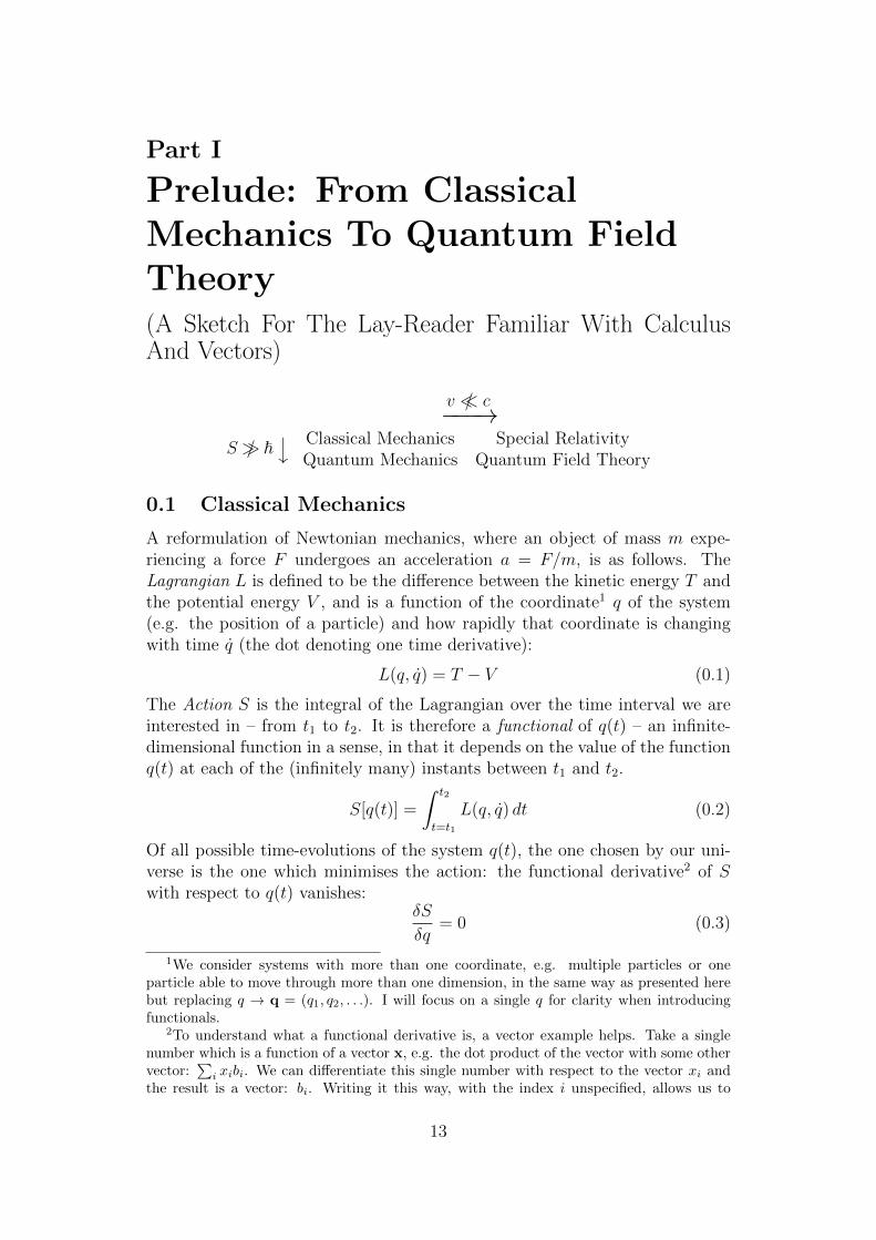
v / c−−−→S / ~

−→ Classical Mechanics Special RelativityQuantum Mechanics Quantum Field Theory

0.1 Classical Mechanics

A reformulation of Newtonian mechanics, where an object of mass m expe-riencing a force F undergoes an acceleration a = F/m, is as follows. TheLagrangian L is defined to be the difference between the kinetic energy T andthe potential energy V , and is a function of the coordinate1 q of the system(e.g. the position of a particle) and how rapidly that coordinate is changingwith time q (the dot denoting one time derivative):

L(q, q) = T − V (0.1)

The Action S is the integral of the Lagrangian over the time interval we areinterested in – from t1 to t2. It is therefore a functional of q(t) – an infinite-dimensional function in a sense, in that it depends on the value of the functionq(t) at each of the (infinitely many) instants between t1 and t2.

S[q(t)] =

∫ t2

t=t1

L(q, q) dt (0.2)

Of all possible time-evolutions of the system q(t), the one chosen by our uni-verse is the one which minimises the action: the functional derivative2 of Swith respect to q(t) vanishes:

δS

δq= 0 (0.3)

1We consider systems with more than one coordinate, e.g. multiple particles or oneparticle able to move through more than one dimension, in the same way as presented herebut replacing q → q = (q1, q2, . . .). I will focus on a single q for clarity when introducingfunctionals.

2To understand what a functional derivative is, a vector example helps. Take a singlenumber which is a function of a vector x, e.g. the dot product of the vector with some othervector:

∑i xibi. We can differentiate this single number with respect to the vector xi and

the result is a vector: bi. Writing it this way, with the index i unspecified, allows us to

13

The solution of (0.3) – the equation(s) of motion – can be obtained by solvingthe Euler-Lagrange equation:

∂L

∂q− d

dt

∂L

∂q= 0, (0.4)

where q and q are considered independent for the partial differentiation. Asan example, the familiar dynamics of a single particle of mass m in a potentialV in one dimension x are obtained from the following Lagrangian:

L = 12mx2 − V (x) (0.5)

(0.4)−−→ mx = −dVdx

(0.6)

This shows how spatial variation of the potential forces the particle to accel-erate towards regions of lower energy.

0.2 Special Relativity

Special relativity tells us that when velocities become relativistic, i.e. non-negligible fractions of the speed of light c, we leave the regime of Newtonianmechanics. A further startling prediction relevant even at non-relativistic ve-locities is that mass is merely another form of energy – the now familiar relation

E = mc2 (0.7)

We can study the relativistic dynamics of individual objects, approximatedas particles: we find that time in a reference frame in motion relative to ourobservations passes more slowly, and that space contracts along the directionof motion. By analogy with the mixing in the directions called ‘left’, ‘right’, ‘infront’ and ‘behind’ as one spins – these quantities are not absolute but dependon the direction one is facing – time and space are not absolute, indeed theyare not even separate: they are mixed together by motion. We can thus thinkof them as separate parts of the same thing: spacetime, xµ=0,1,2,3 = (t,x) =(t, x, y, z).

The context of special relativity is a good one to introduce the concept ofa field. Essentially, a field is just something which is a function of position inspace: in our three dimensions of space, it’s a function of x, y and z, and it canalso change with time. A scalar field is a field characterised by a single numberas a function of space and time. For example, one could describe the spatialand temporal variation of temperature with a scalar field – one number at eachpoint, giving the local temperature at that moment. A vector field is a field

express simultaneously the different results that arise when we choose to differentiate withrespect to different components of the vector x. A function q(t) is an infinite-dimensionalvector of sorts – there is a different value associated with each ‘index’ t, with t continuous.By analogy with the vector example, when we differentiate a functional with respect to afunction, the result – a functional derivative – is a function.

14

characterised by a vector – that is to say a single number with an associateddirection, or equivalently a set of numbers – as a function of space and time. Anexample is the gravitational field: everywhere in the space around a planet, ora star (everywhere at all in fact), there is a number characterising how stronggravity is there, and a direction that the force acts in. A localised disturbancein a field may propagate elsewhere as a wave, or it may simply slowly recoverto how it was before. Compare prodding the surface of water to prodding thesurface of treacle.

The behaviour of fields can be captured quantitatively using a Lagrangiandescription as in Section 0.1. Where previously the Lagrangian was a simplefunction of the system’s coordinate q and its time derivative q, now it is anintegral over the spatial region of interest V of a quantity defined at each pointin space: the Lagrangian density L, with density meaning per unit volume. Lis a function of the field and its spacetime derivatives; the latter are obtainedwith the operator ∂µ = ∂

∂xµ. For example, for a scalar (just one number) field

φ in three spatial dimensions x:

φ = φ(xµ)

L = L(φ, ∂µφ)

L =

∫x∈VL d3x

(0.8)

Otherwise the equations of motion are obtained almost exactly as in the pre-vious section:

S[φ] =

∫ t2

t=t1

Ldt =

∫ t2

t=t1

∫x∈VL d4x, (0.9)

δS

δφ= 0 (0.10)

=⇒ ∂L∂φ−∑µ

∂µ∂L

∂(∂µφ)= 0 (0.11)

As we take t1 → −∞, t2 → +∞ and V to be all of three-dimensional spaceV → R3, in other words if we are interested in all spacetime, the action isa Lorentz invariant – the same number for all observers regardless of theirrelative motion.

An Example: a free (non-interacting), massive scalar field φ:

L =∑µ,ν

12gµν∂µφ ∂νφ− 1

2m2φ2 (0.12)

(0.11)−−−→∑µ,ν

gµν∂µ∂νφ+m2φ = 0, (0.13)

where gµν is the metric of spacetime, which defines how to contract two space-time vectors together to obtain a Lorentz invariant3: it is the diagonal 4 × 4

3A more familiar example of this kind of object is the metric of ordinary three-dimensional

15

matrix gµν = gµν = diag+1,−1,−1,−1. We can solve (0.13) by first takingthe Fourier transform of φ(xµ): expressing it as an arbitrary linear superposi-tion (actually integrating rather than summing) of exp(i

∑µ,ν gµνp

µxν) termswith i is the imaginary number

√−1. Plugging this into (0.13) we find the

constraint that pµ = (√

(m2 + p2),p), with p = (px, py, pz) arbitrary and thelinear superposition of terms still arbitrary. Each term in this superpositiontaken singly represents a wave with wave-vector/momentum p and an associ-ated energy E =

√(m2 + p2).

Note that the energy does not vanish as the momentum vanishes: Ep→0−−→ m.

This energy gap between the vacuum (zero energy) and the lowest energy mode(the limit p → 0) is the mass of the field. The situation is the same as forparticles: there is a minimum energy E = mc2 needed to create a stationaryparticle, and further energy becomes its kinetic energy.

0.3 Quantum Mechanics

If all speeds that we encounter in our problem are well below c, we do notneed to worry about extending classical mechanics with special relativisticeffects. However if we consider actions (recall Eq. (0.2)) so small that they’recomparable to the fundamental constant of nature ~ – the reduced Planckconstant – we enter the realm of quantum mechanics. Here we discover thatthere is an inherent uncertainty at the microscopic level; for example a particlecannot possess a well-defined position and momentum simultaneously. Thestate of a system is described by a wave function, often denoted |ψ〉. Fora single particle this could be a probability distribution for its position andmomentum. We associate with each physical observable an operator4. It is alaw of quantum mechanics that any time we measure a property of a system, we

space, the three-by-three unit matrix gij = diag+1,+1,+1. When we contract two vec-tors together with this metric, a.b =

∑i,j gija

ibj =∑i aibi, the result is invariant under

rotations of the space, i.e. SO(3) transformations.4A function is something which takes a number and returns another number; e.g. “2x”

takes any number and returns that number doubled. An operator, simply understood,takes a function and returns another function; e.g. “d/dx” takes any function of x andreturns the first derivative. This definition of an operator makes sense in the quantummechanical context when we consider wave functions |ψ〉 that are simple functions, such asposition/momentum probability distribution functions: the operator acting on |ψ〉 returnssome other function. We may consider wavefunctions that are less readily understood assimple functions, however, such as those describing a particle’s intrinsic spin. In this contextthe more general definition of an operator – a mapping from one vector space to another –is appropriate: a quantum mechanical operator is a mapping from the space of all possiblewavefunctions onto that same space (but not necessarily the same point in that space!). Theeigenvectors of an operator are points in the relevant space which are mapped back ontothemselves, multiplied by a constant called the eigenvalue. For example all points on the zaxis are eigenvectors of the operator in three-dimensional space “rotate around the z axis”with eigenvalue 1 (note that points away from the z axis are not eigenvectors). Anotherexample is the operator “d/dx”, whose eigenvectors are ekx (with k any constant) witheigenvalue k.

16

can only observe states of the system that are eigenvectors of the correspondingoperator, and the result of our measurement is the associated eigenvalue. Asan example, the intrinsic spin of a fermion such as an electron may be alignedwith whatever direction we decide to call the positive z axis – the state | ↑〉 –or in the opposite direction – | ↓〉 – or it may be a linear combination of thesetwo possibilities. | ↑〉 and | ↓〉 are eigenstates of the z-axis spin operator sz:

• sz| ↑〉 = +12| ↑〉,

• sz| ↓〉 = −12| ↓〉,

• but sz(| ↑〉+ | ↓〉) = +12| ↑〉− 1

2| ↓〉 6= constant× (| ↑〉+ | ↓〉), so this state

is not an eigenstate of sz and in measuring the z-axis spin we will neverobserve this state. If the system really is in this state, then when wemeasure the z-axis spin we force it to change state either into | ↑〉 or into| ↓〉: this forced change is referred to as the collapse of the wavefunction.How (or indeed if) this really happens has been the subject of muchdebate, known as the measurement problem.

In general when the system is in a state |ψ〉 and we want to know theprobability of finding it in the particular state |φ〉 (a probability which is notnecessarily 0 by definition, since |ψ〉 may be a superposition of states, oneof which is |φ〉), this probability is |〈φ|ψ〉|2. The quantity 〈φ|ψ〉 is highlyanalogous to taking the dot product of two vectors to quantify how much theyoverlap; indeed |ψ〉 and |φ〉 are vectors in the (possibly infinite-dimensional)space of all possible states the system can be in.

Time evolution of a state |ψ〉 occurs according to the Schrodinger equation:

∂

∂t|ψ〉 = − i

~H|ψ〉, (0.14)

where H is the Hamiltonian – the operator whose eigenvalues are the possibleenergies the system (which are sometimes discrete, e.g. the energy levels ofelectrons in atoms). From Eq. (0.14) we see that if the system is in a state ofdefinite energy – it is an eigenstate of H with eigenvalue E – its dependenceon time is simply given by a factor exp(−iEt). If |ψ〉 is not a state of definiteenergy, we can still write down a solution to Eq. (0.14) with the correct timedependence by inspection:

|ψ(t = T )〉 = exp

(− i~HT

)|ψ(t = 0)〉 (0.15)

However understanding what this solution really means may be highly non-trivial because in general H is the sum of non-commuting5 operators.

5If operators A and B do not commute, this means AB 6= BA. This is a strange conceptat first because we’re mostly used to normal numbers, and 2×3 = 3×2, but A could be the

17

If at a time t = 0 a particle has definite position q1, a state we call |q1〉,then at a later time T the state of the system is

|ψ(t = T )〉 = exp

(− i~HT

)|q1〉 (0.16)

The probability to observe the particle at a definite, different position q2 atthis later time is

|〈q2|ψ(t = T )〉|2 =

∣∣∣∣〈q2| exp

(− i~HT

)|q1〉∣∣∣∣2 (0.17)

A gorgeous piece of mathematics shows that contents of the | . . . |2 can beevaluated as a path integral:

〈q2| exp

(− i~HT

)|q1〉 =

∫ q(t=T )=q2

q(t=0)=q1

eiS[q]/~ Dq, (0.18)

where we integrate over the infinite number of possible functions of time q(t)in the interval t ∈ [0, T ] subject to the boundary conditions q(t = 0) = q1 andq(t = T ) = q2. In a sense this is an infinite-dimensional integral, since thespace of possible functions is infinite dimensional.

0.4 Quantum Field Theory

Non-relativistic quantum mechanics describes the time evolution of quantumsystems – particles moving, changing their intrinsic spin etc. – without al-lowing for the creation or destruction of particles. Constant particle numberis hard-coded in the theory. However special relativity tells us that mass ismerely another form of energy, and therefore particles can be created and de-stroyed. Quantum field theory (QFT) extends quantum mechanics to includethis new feature, and makes the physical laws Lorentz invariant. Central tothe idea of QFT is that there exists a field, permeating the whole of space,for each kind of fundamental particle; a single particle is simply a localisedexcitation of its field, able to propagate through space.

The surface of a body of water can be described by a field (height as afunction of position) which can have two opposite kinds of excitation – peaksand troughs – both with positive energy but which are able to cancel each otherout. The same is true of the fundamental particle fields – they may supportboth particle and antiparticle excitations, and pairs of these may annihilate

operation ‘rotate an object 90 left’ and B the operation ‘rotate an object 90 forwards’.You can see for yourself with whatever object you have to hand that the order in which theseoperations are performed matters. In the context of quantum mechanics, a bit of simplemaths shows that two operators representing two physical properties that cannot both takedefinite values simultaneously, such as position and momentum, must not commute; andindeed the position and momentum operators generally feature in the Hamiltonian.

18

into pure energy or be produced out of pure energy. Note that this pictureof antiparticles is fundamentally different from (though often gives similaranswers to) the older description in terms of a Dirac sea. The latter consistsof a vacuum which is an infinite number of negative energy particle statesall filled, and no positive states filled; antiparticles are then interpreted asavailable negative energy states, which can annihilate particles in an intuitiveway.

In QFT the kinds of objects we wish to compute resemble those of normalquantum mechanics – probability amplitudes for a given initial state to laterbe observed as a given final state (see the glossary). A result familiar fromthe description of mundane every-day waves is that energy is inversely relatedto distance – higher energy waves have smaller wavelengths – and thereforeto understand nature at ever smaller length scales, the relevant processes forour calculation of probability amplitudes are those in which large amounts ofenergy are exchanged. Of course we must actually carry out these processes aswell, so that our calculations, and the theories that define them, can be tested.In practice this is done by colliding particles together as hard as we can, thenrecording the relative number of occurrences of the different final states thatresult (i.e. establishing probability distributions for the final states). Hencethe initial states for our calculations generally consist of two particles travellingtowards each other at a high relative velocity; the final states considered willbe everything that those two particles can produce after interacting with eachother in an arbitrary way6. As with the quantum mechanical path integral,the probability amplitude for a transition between given states can be calcu-lated as the integral of exp(iS/~) over the space of all possible things thatcould have happened during the transition. However previously this objectwas simpler: the integral was over all possible functions of time the coordi-nate could take, q(t). Now our transition is from two localised excitations offields, to some other number of localised excitations, and the associated fieldscould do anything in between times: for each of these fields (and indeed anyother field that interacts with them), we must integrate over all possible be-haviours as a function of time for each point in space! In other words we havean infinite-dimensional integral of the form Eq. (0.18) associated with each ofthe infinitely many points in continuous space.

These tremendously daunting mathematical objects have been computedexactly in certain theories simpler than those of direct relevance to our universeand our current particle colliders. In the latter cases, we typically have to resortto an expansion of the probability amplitude (that is, a systematic groupingof the infinite number of contributing terms into a series consisting first ofthe largest then the second largest etc. ad infinitum) followed by a truncatedcalculation of as much of the series as we are able to do in a given number

6Note that not everything is possible – conservation rules such as the conservation ofenergy, momentum and electric charge imply that the final state must have the same valuesfor these quantities as the initial state.

19

of man-hours. Each term in the expansion can be represented by a Feynmandiagram, with the translation between diagram and term established by aset of universal Feynman rules. Crudely speaking, the simpler the Feynmandiagram – the smaller the number of intermediate, localised excitations of thefields connecting the initial configuration of fields (two incoming particles) tothe final one – the larger the term it represents. This is because connecting theinitial and final states with an increasing number of interactions between fieldsusually means, via the Feynman rules, that the term has an increasingly smallpre-factor. Sometimes this is not the case, when the coupling between fields is‘strong’ (meaning strong enough to compensate for the small pre-factor); thenthe terms at each step of the expansion are as big as those preceding them,and without the ability to sum the entire infinite series we lose calculability.In the author’s opinion, this is the greatest unsolved problem in mathematicalphysics.

An important difference between QFT and classical field theory is that theparameters appearing the in the Lagrangian density L no longer relate directlyto physical observables in the same way. For example, the dimensionless num-ber multiplying a term containing two or more different fields (thus allowingthe respective particles to interact), known as a coupling or coupling constant,does not quantify the interaction strength, or at least not in a simple way. Therelations between the parameters of L and their corresponding observables nowcontain infinities, which have to be subtracted by hand in such a way as toleave a set of parameters that agree with the experimentally established valuesby construction. Note that choosing the parameters of a model of nature inorder to reproduce what is known to be true is often regarded as a bad thing,as science should make predictions that allow for falsification. However pre-dictivity is only lost when there is enough flexibility in the model parametersto accommodate any experimental result; in the case of QFT there are consid-erably more observables than those corresponding directly to the parametersof L, and these are genuine predictions, which match known measurements toa simply stunning level of precision.

The removal of infinities to set the parameters of L, known as renormali-sation, must be done at a particular energy scale. An extremely deep featureof QFT is that, once this has been done, a different set of parameters is appro-priate for describing particle interactions at a different energy scale; in otherwords, the renormalised (infinity-subtracted) parameters of L run with energyscale. The coupled differential equations controlling this running – the renor-malisation group (RG) equations – are an example of something predictedby a given QFT, once each of the parameters of L has been defined at onescale. The physical picture often used to summarise the positive running ofthe electromagnetism coupling is the following. In probing a charged point-likeparticle with a low-energy photon, one is really probing only the rough area ofspace the charge is sitting in, due to the photon’s long wavelength. This spacealso contains virtual charged particle-antiparticle pairs by virtue of quantum

20

uncertainty, with the opposite charges tending to lie closer to the real physicalparticle (in the usual manner of polarisable media), shielding the charge that iseffectively seen. This effect decreases the smaller the wavelength of the photon,hence the increasing strength of the electromagnetic coupling with energy.

21

Part II

Weak-Scale Susy’s Raisond’Etre: The Higgs

1 Introduction

1.1 Motivation

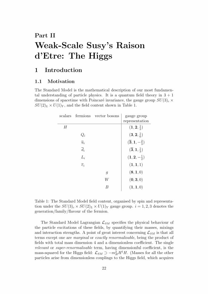
The Standard Model is the mathematical description of our most fundamen-tal understanding of particle physics. It is a quantum field theory in 3 + 1dimensions of spacetime with Poincare invariance, the gauge group SU(3)c ×SU(2)L × U(1)Y , and the field content shown in Table 1.

scalars fermions vector bosons gauge grouprepresentation

H (1,2, 12)

Qi (3,2, 16)

ui (3,1,−23)

di (3,1, 13)

Li (1,2,−12)

ei (1,1, 1)

g (8,1, 0)

W (0,3, 0)

B (1,1, 0)

Table 1: The Standard Model field content, organised by spin and representa-tion under the SU(3)c × SU(2)L × U(1)Y gauge group. i = 1, 2, 3 denotes thegeneration/family/flavour of the fermion.

The Standard Model Lagrangian LSM specifies the physical behaviour ofthe particle excitations of these fields, by quantifying their masses, mixingsand interaction strengths. A point of great interest concerning LSM is that allterms except one are marginal or exactly renormalisable, being the product offields with total mass dimension 4 and a dimensionless coefficient. The singlerelevant or super-renormalisable term, having dimensionful coefficient, is themass-squared for the Higgs field: LSM ⊃ −m2

HH†H. (Masses for all the other

particles arise from dimensionless couplings to the Higgs field, which acquires

22

a non-zero vacuum expectation value (VEV) v.) This term is at the heart of aproblem the Standard Model is widely believed to suffer from: unnaturalness.

’t Hooft argued that a small parameter of the Lagrangian is naturally smallif the Lagrangian has an enhanced symmetry when the parameter vanishes [1].In that limit, the symmetry forces the radiative corrections to vanish, andso with the parameter non-zero the corrections must be proportional to theparameter itself. This is sometimes referred to as technical naturalness. Forexample, small electron masses in quantum electrodynamics are technicallynatural because chiral symmetry in the massless limit enforces

δm ∝ m (1.1)

However if we have a fundamental scalar φ then, outside of conformally invari-ant theories, allowing its mass-squared to vanish does not enhance the sym-metry; indeed explicitly calculating the radiative corrections one finds termslike

δm2φ ⊃

g2

16π2Λ2, (1.2)

where g is the coupling of φ to a particle that can run in a loop of the two-point correlator 〈φ(−p)φ(p)〉, and Λ is an ultraviolet (UV) cutoff for the di-vergent integral. The hierarchy problem can be loosely phrased in the fol-lowing way: if Λ2 is parametrically larger than the renormalised mass-squaredm2φ = m2

φ,bare+δm2φ, the cancellation on the right-hand side (RHS) of this equa-

tion between the bare value and radiative corrections requires parametricallylarge fine-tuning; otherwise we would expect m2

φ = O( (g2/16π2)Λ2). However,if Λ is to be understood as nothing more than a non-physical regulator to betaken to infinity, our question is not well posed. This leads us to the moreprecise technical hierarchy problem, which we have when Λ is interpreted as aphysical cutoff, below which our theory is an effective theory. When we enterthe regime of the latter by integrating out heavier degrees of freedom at thescale Λ, there will generically be corrections of this size to any scalar masses,suppressed by however many loop-factors are necessary to couple the scalar tothese heavy particles7. Unless there is no new physics coupling to the Higgs atany higher energy scale, we then return to the conclusion of the simple hierar-chy problem that the Higgs mass should be O( (g2/16π2)Λ2). More concretely,in the Standard Model we have a mass-squared O(100 GeV)2 and a correction(y2t /8π

2) Λ2 from the large coupling yt of the Higgs to the top-quark. We wouldtherefore require a cutoff Λ ∼

√(8π2/y2

t ) 100 GeV = O(1 TeV). Taking thecutoff instead to be the Planck mass MP ∼ 1018 GeV – the highest scale atwhich the Standard Model without quantum gravity could be valid – requiresfine-tuning to one part in ∼1030.

7One might consider new physics at a scale Λ which does not couple to Higgs at any orderin perturbation theory; it would therefore not couple to any part of the Standard Model –a fairly uninteresting scenario. Gravity at least must couple to the Higgs, as the latter hasmass and energy.

23

The requirement for new physics fully explaining naturalness can be pushedfrom 1 TeV to higher energies if the Higgs is a pseudo-Nambu-Goldstone boson(pNGB); I briefly review the idea of these little Higgs models in Appendix A.(Note however that this still requires some new physics at the TeV scale –specifically top partners – to cancel the top quark correction to the Higgsmass.) Full explanations of naturalness, traditionally considered at the TeVscale (rather than at the higher scale permitted by little Higgs) generally fallinto one of the three following camps. For the first two I will merely state theidea without explaining details; a nice introduction to all three can be foundat [2], and there are several different sets of TASI lecture notes available onthese topics.

Firstly, quantum-gravitational effects effects may become relevant, requir-ing extra dimensions. The Higgs could be the fifth component of a five-dimensional gauge field; masslessness in the limit of the fifth dimension be-coming large and flat means the Higgs is naturally light. Alternatively it couldbe a fundamental scalar confined to a physical four-dimensional subspace – abrane – with an effective momentum cutoff resulting from the extra dimensionsbeing warped [3].

Secondly, the Higgs may be composite, i.e. (extensions of) the idea ofTechnicolour. It is a bound state of a fermion and an anti-fermion (techni-quarks), which are confined by a new gauge group. Techniquark condensation(i.e 〈qTCqTC〉 becoming non-zero) spontaneously breaks the global SU(2)L ×SU(2)R symmetry of the techniquarks to the diagonal SU(2)V giving threewould-be Nambu-Goldstone bosons (NGBs) – technipions, by close analogywith regular pions – which the hungry massless W and Z bosons eat insteadof the three would-be NGBs in the H doublet in the Standard Model. Tech-nicolour in particular is more attractive with a little Higgs setup than with-out [4, 5].

Thirdly, and finally moving to the topic of this thesis, a light fundamentalscalar may be protected by Supersymmetry (see [6] for an extensive introduc-tion, review and many references; also [7, 8] for preliminaries), henceforth Susy.Susy generators convert bosons into fermions and vice-versa; a supersymmet-ric theory must therefore be constructed from objects called superfields, inwhich half the degrees of freedom are bosonic and half are fermionic; each halfis said to be the superpartner of the other, with exactly the same quantumnumbers excepting spin. In such theories, radiative corrections to the mass-squareds of scalars vanish at every order in perturbation theory: bosonic andfermionic loops always come in pairs, with the same magnitude but oppositesign. With Susy broken, but only softly – that is, where superpartners havedifferent dimensionful ‘couplings’ (including mass) but identical dimensionlesscouplings – quadratic divergences still vanish, since the associated couplingconstant must be dimensionless for the diagram to have dimension two. Thereare still logarithmically divergent corrections associated with the effective the-ory where one particle has been integrated out but its superpartner has not;

24

such corrections are proportional to the scale of soft Susy breaking. In thismanner we may have a light Higgs naturally.

Motivations for considering our universe to be supersymmetric are as fol-lows.

1. The (technical) hierarchy problem as discussed.

2. The symmetry group for our physical laws increased in size until we ar-rived at the Poincare group. Coleman and Mandula’s no-go theorem [9]‘proved’ (for a while) that there are no non-trivial extensions of thisgroup, i.e. that any extension would be the direct product of the Poincaregroup and internal (non-spacetime) symmetries. Haag, Lopuszanski andSohnius [10] found the loop-hole: non-trivial extensions are allowed butonly with fermionic symmetry generators, i.e. Susy. Susy is thus unique,in a fairly profound way, among possible extensions of the StandardModel. Intimately tied up with this feature is the widely believed unique-ness of Susy (or more precisely its generalisation from a global to a localsymmetry – Supergravity) as a setting in which a spin-3

2particle may

exist (see e.g. [11, 12]).

3. Susy is widely believed to be a requirement of consistent string theory,and the latter is widely believed to be the correct framework for a de-scription of gravity at the quantum level. The necessary existence of thelatter is thus a motivation for Susy.

4. The three independent gauge couplings of the Standard Model, whenevolved using the renormalisation group (RG) to an energy scaleO(1016 GeV), almost meet at a point. This suggests the tempting possi-bility that with extra charged matter added at lower scales, they really domeet (which tends to happen in Susy) and there is only one fundamentalgauge group: Grand Unification. There is strong historical motivationfor us to explain more phenomena with fewer principles. Proposing amuch enlarged field content, as we’ll see shortly is necessary, to solvethe one-parameter problem of making three lines meet at a point soundslike overkill. However in Grand Unified Theories (GUTs) there is an ex-tremely large scale with new physics that couples directly to the Higgs,thus removing any doubt about the applicability of the technical hierar-chy problem. Grand Unification thus motivates Susy for two reasons:

(a) the superpartners modify the RG running of the gauge couplings ina way that generally improves the extent to which they meet at asingle scale; and

(b) we fall squarely into the scope of the technical hierarchy problem,and with Susy the unavoidable, physical, O(1016 GeV)2 contribu-tions to the Higgs mass-squared sum to zero.

25

5. There is overwhelming evidence from astrophysical observations for theexistence of a new neutral particle which is stable on cosmological time-scales – dark matter, see for example [13] for a review. Often we imposea discrete Z2 symmetry called R parity on Susy theories in order tosuppress terms which would strongly violate experimental bounds onproton stability. With R parity, the lightest new particle with oppositecharge to the Standard Model particles – the Lightest SupersymmetricParticle (LSP) – is stable; if it is also neutral it is a dark matter candidate.However introducing Susy and the plethora of necessary particles solelyfor one of them to be dark matter is overkill – this problem may beaddressed more minimally than the (technical) hierarchy problem, oneexample being with the Peccei-Quinn axion which also solves the strongCP problem [14, 15].

6. On July 4th 2012 the ATLAS and CMS Collaborations announced theirindependent discoveries at roughly 5σ confidence level of a new bosonicresonance, with properties as measured so far coinciding closely with theHiggs of the Standard Model, and mass ∼126 GeV [16, 17]. Now, Susy isa broad collection of different theories with different properties; howeverwhat’s common to almost all of them is that the Higgs mass mh is con-nected to the electroweak gauge boson masses ∼MZ , and enjoys a specialprotection from radiative corrections. The authors of [18] studied mh inboth split Susy [19, 20, 21, 22] and high-scale/supersplit Susy [23], bothof which are versions of the Minimal Supersymmetric Standard Model(MSSM, see Section 1.3). Split Susy decouples all scalar superpartnersof the Standard Model fermions while leaving all fermionic superpartnerslight (with the possible exception of those of Higgs, according to taste);high-scale Susy decouples all non-Standard Model particles. The findingof [18] was that even sending superpartner masses to the Planck scale,mh remains below 157 (143) GeV in split (high-scale) Susy. The impor-tance of this result, beyond showing which models have mh ≈ 126 GeVand which do not, is as an illustration of the robustness of the MSSMprediction for mh = O(MZ): low-scale Susy gives both electroweak nat-uralness and mh = O(MZ); in decoupling Susy we lose the former andthus part of the motivation, but we are still left with the latter. This isto be contrasted with the Standard Model, for which the prediction wasmh . 700 GeV for perturbative unitarity of WW scattering at the TeVscale. From this point of view, Susy (or more precisely the MSSM andits not-too-distant cousins) gave a slightly better prediction for mh thanthe Standard Model.

Note that points 1 and 4b motivate weak-scale Susy; points 4a and 5 have aslight preference for at least some Susy particles at the weak scale; points 2, 3and 6 motivate Susy but without a preference for its breaking scale, whichcould be anywhere up to MP .

Having motivated Susy, I now give a brief explanation of what it is.

26

1.2 The Superpotential

(See [8, 6] for much more thorough explanations than the sketch given here.)As I have mentioned, a supersymmetric theory should be built from superfields.Superfields can be considered simply as book-keeping devices, as they pair upbosonic and fermionic fields with otherwise identical quantum numbers. Moreformally they are functions of superspace, X ≡ (xµ, θα, θα), where θα=1,2, θα=1,2

are two-component spinors of anti-commuting Grassman variables. The mostgeneral function of X, expanded in powers of θ and θ with xµ-dependentcoefficients, is of finite length: Grassman variables are nilpotent – they vanishwhen squared. This polynomial is a reducible representation of the group ofSusy transformations, and irreducible representations (irreps) can be made bytaking subsets of the finite number of terms. Two such irreps are left-handedand right-handed chiral superfields, each of which contains a single complexscalar, a fermion of the denoted chirality, and an unphysical/auxiliary scalarF . Expanding a left-handed superfield Φ in powers of θ and θ, the coefficientof the θαθα term is F ; then following the rules of Grassman integration,∫

d2θ Φ = F (1.3)

Under a Susy transformation F can be seen to change by a total derivative, andso an action defined from a Lagrangian consisting of F -terms will be invariantunder Susy transformations. The product of left- (right-) handed superfieldstransforms itself like a left- (right-) handed superfield under the Susy group,and so the following Wess-Zumino Lagrangian is supersymmetric:

L =

∫d2θ W (Φ) + c.c., (1.4)

where W (Φ) ≡ χiΦi +MijΦiΦj + yijkΦiΦjΦk (1.5)

The quantityW (Φ) is the superpotential – a holomorphic dimension-three func-tion of all the left-handed chiral superfields Φi in the model. Writing the scalarin Φi as φi, and with W (φ) the same function of these scalar fields as W (Φ) isof the corresponding superfields, the contribution of the superpotential to theregular potential V (φ) is

V (φ) ⊃∑i

∣∣∣∣∂W (φi)

∂φi

∣∣∣∣2 (1.6)

where this has come from Eq. (1.4) followed by a replacement of each non-physical F field by the solution of its (algebraic) equation of motion; the termson the RHS are thus referred to as F -terms.

The other contributions to the potential come from so-called D-terms,which arise from supersymmetric gauge interactions. Spin-one vector bosonsassociated with gauge symmetries live inside a different representation of theSusy group called a vector superfield, with a fermionic partner called a gaugino

27

and an auxiliary scalar D field. The coefficients in front these different compo-nent fields in the Lagrangian are fixed by Susy; however in the specific case ofa vector superfield for an abelian gauge symmetry, we can add to Lagrangianan arbitrary extra amount of the associated D field: L ⊃ kD. This is theFayet-Iliopoulos term [24]. Arranging all of the φi in the theory into a vectortransforming in a (possibly reducible) representation of the full gauge groupwith generators T a, the D-terms are

V (φ) ⊃ 12

∑a

(ga φ†iT

aijφj + ka)2, (1.7)

where the gauge coupling ga is of course common to different generators ofthe same gauge symmetry, but if the full gauge group is a product of differentgroups there is one coupling for each of these groups.

1.3 The MSSM

To supersymmetrise the Standard Model we must place each of its fields (shownin Table 1) into a superfield, and include one more superfield [25, 26], expand-ing the set of degrees of freedom to those shown in Table 2. Each row (i.e. eachsuperfield) in Table 2 except the second one contains a field as in the StandardModel, with a new bosonic or fermionic partner. The second row, Hd and Hd,is the new superfield. This is required, forcing us into a two-Higgs-doubletmodel, for two reasons. Firstly the Standard Model mechanism of generatingmasses for the charged leptons and down-type quarks through a coupling withcomplex conjugate of the Higgs doublet is not possible due to the requirementthat the superpotential be holomorphic. Secondly, our introduction of the Hu

fermion violates the SU(2)L × U(1)Y gauge anomaly cancellation conditions;they are restored with an extra fermion of opposite hypercharge Y , such asHd.

The superpotential of the R parity conserving MSSM is

WMSSM = yu,ijuiQjHu − yd,ij diQjHd − ye,ij eiLjHd + µHuHd, (1.8)

where, with the standard abuse of notation, the same symbol is used for asuperfield and its scalar component (for the Higgs fields) or fermionic com-ponent (for the Standard Model fermions). In Eq. (1.8) SU(2)L and SU(3)cgauge indices within each term are implicitly contracted to form a singlet.

The fermionic partners of the Higgs scalars and vector bosons are calledHiggsinos and gauginos respectively, with the latter consisting of a bino, winosand a gluino. The scalar partners of Standard Model fermions take the nameof the corresponding fermion with the letter ‘s’ prepended: for example theleft- and right-handed stops tL,R are the scalar partners of the left- and right-handed chiralities of the top quark, and we define the sfermions and sleptonsetc. similarly. Non-Standard Model particles are collectively called sparticles.

In the two, complex, scalar Higgs doublets there are eight degrees of free-dom. Three of these are the would-be NGBs that become the longitudinal

28

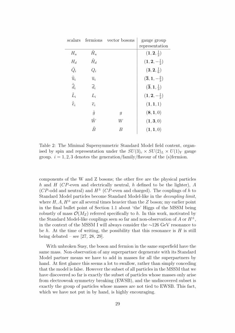
scalars fermions vector bosons gauge grouprepresentation

Hu Hu (1,2, 12)

Hd Hd (1,2,−12)

Qi Qi (3,2, 16)

ui ui (3,1,−23)

di di (3,1, 13)

Li Li (1,2,−12)

ei ei (1,1, 1)

g g (8,1, 0)

W W (1,3, 0)

B B (1,1, 0)

Table 2: The Minimal Supersymmetric Standard Model field content, organ-ised by spin and representation under the SU(3)c × SU(2)L × U(1)Y gaugegroup. i = 1, 2, 3 denotes the generation/family/flavour of the (s)fermion.

components of the W and Z bosons; the other five are the physical particlesh and H (CP -even and electrically neutral, h defined to be the lighter), A(CP -odd and neutral) and H± (CP -even and charged). The couplings of h toStandard Model particles become Standard Model-like in the decoupling limit,where H,A,H± are all several times heavier than the Z boson; my earlier pointin the final bullet point of Section 1.1 about ‘the’ Higgs of the MSSM beingrobustly of mass O(MZ) referred specifically to h. In this work, motivated bythe Standard Model-like couplings seen so far and non-observation of A or H±,in the context of the MSSM I will always consider the ∼126 GeV resonance tobe h. At the time of writing, the possibility that this resonance is H is stillbeing debated – see [27, 28, 29].

With unbroken Susy, the boson and fermion in the same superfield have thesame mass. Non-observation of any superpartner degenerate with its StandardModel partner means we have to add in masses for all the superpartners byhand. At first glance this seems a lot to swallow, rather than simply concedingthat the model is false. However the subset of all particles in the MSSM that wehave discovered so far is exactly the subset of particles whose masses only arisefrom electroweak symmetry breaking (EWSB), and the undiscovered subset isexactly the group of particles whose masses are not tied to EWSB. This fact,which we have not put in by hand, is highly encouraging.

29

The general tree-level vanishing [30] of the supertrace

STrM2 ≡∑

all particles

(−1)s(2s+ 1)M2 = 0 (1.9)

where M is a particle’s mass and s its spin, means that spontaneous breaking ofSusy from within the MSSM will be phenomenologically unacceptable – somesuperpartners will be lighter than their Standard Model partners, whereaswe need them all to be heavier. Susy breaking must therefore be a higher-order/quantum effect, mediated to the MSSM from elsewhere – the hidden sec-tor. The three main approaches to achieving the mediation are through grav-itational interactions, extra dimensions, or gauge interactions (see Part III).

Susy breaking results in mass-squareds m2φ and Majorana masses Mλi

for

all of the scalars φ = Hu.Hd, Qi, ui, di, Li, ei and gauginos λi = B, W , g respec-tively in Table 2. It also gives the trilinear mixing terms L ⊃ −uiau,ijQjHu +

diad,ijQjHd + eiae,ijLjHd + c.c.; each aij matrix is usually assumed to be pro-portional to the corresponding Yukawa matrix. In the basis where these arediagonal, we have for example a33 = ytAt; the stop trilinear mixing parameterAt gives potentially large corrections to the physical Higgs mass as we willsee in the following section. The final term arising from Susy breaking is thedimension-two mixing term for the Higgs scalars L ⊃ −bHuHd + c.c..

In addition to the Susy breaking masses there is a single supersymmetricmass parameter in the MSSM, for the two Higgs superfields: the µ term. Thiscompletes the list of dimensionful terms in the MSSM. Those relevant for thetwo CP -even electrically neutral scalars H0

u and H0d are:

V ⊃ (H0u (H0

d)∗)

(|µ|2 +m2

Hu−b

−b |µ|2 +m2Hd

)((H0

u)∗

H0d

)(1.10)

For EWSB one linear combination of H0u and H0

d must have a negative mass-squared to destabilise the origin. The resulting VEV then lies partly alongthe H0

u direction and partly along the H0d direction, and is characterised by

tan β = vu/vd. It is instructive (and motivated – see Section 2) to considerlarge tan β 1; in this limit H0

u alone corresponds to the single CP -even andneutral degree of freedom in the Standard Model H doublet. Its (negative)mass-squared – the upper-left entry of the matrix in Eq. (1.10) – then leadsto all Standard Model masses. For example we have

− 12M2

Z = m2Hu + |µ|2 +O((tan β)−2). (1.11)

An appealing feature of Susy, once it is broken, is the possibility of radiativeEWSB. Even if m2

Huis positive at the high-scale Λ where mediation of Susy

breaking to the visible sector takes place, Hu couples to the top sector viathe large top Yukawa coupling resulting in a strong tendency for m2

Huto be

pushed negative by RG evolution from Λ to the electroweak scale. This strongradiative correction of m2

Humotivates us to write this explicitly it as

− 12M2

Z = m2Hu(Λ) + δm2

Hu + |µ|2 +O((tan β)−2). (1.12)

30

With this equation we are ready to discuss naturalness.

1.4 Naturalness Under Pressure

Probably the most common measure of naturalness or fine-tuning is the Barbieri-Giudice measure [31], which can be calculated for UV-complete models wherea set of fundamental parameters pi set all of the masses at the scale Λ. Fora given point in pi space that results in the observed value of MZ (throughEq. (1.12)), one calculates derivatives of logMZ with respect to log pi; MZ

is taken to be natural if all such derivatives are . O(1) – doubling a funda-mental parameter at most doubles the resulting MZ . If one of the derivativesis considerably larger than this, the associated pi needs to be finely tuned toproduce the observed MZ . However this measure does not penalise a situationthat we should still regard as unnatural.

If a single parameter p sets both m2Hu

(Λ) and all of the (most important)masses involved in the radiative correction δm2

Hu, it could set these in such

a pattern that m2Hu

(Λ) and δm2Hu

happen to cancel each other out even ifeach term separately is very large, and we have insensitivity of MZ to theparameter p. This is known as focus-point Susy. However the cancellationdepends sensitively not only on this mass-setting pattern but also on the valueof the top Yukawa8, and weakly on the scale Λ; unless these three are linked bysome symmetry the cancellation is accidental. A natural theory, by contrast,does not have large cancellations except those enforced by symmetries. (Highsensitivity to the imprecisely known top mass also makes it uncertain whethersuch models have EWSB at all [32].)

A stricter criterion for naturalness is simply to ask that none of the termscontributing to the right-hand side of Eq. (1.12) are dramatically larger than12M2

Z , in the manner of Kitano and Nomura [33]. This has the further ad-vantage of allowing bottom-up deductions to be made, i.e. without knowingthe underlying high-scale theory, for example as was done in [34] to lay outrequirements on a natural spectrum.

The stop is the chief contributor to δm2Hu

, and thus we require light stopsfor naturalness. We can also see this intuitively – the Standard Model Higgscouples most strongly to the top, so to protect it from strong radiative correc-tions we want Susy broken as weakly as possible in the top sector. Searches atthe Large Hadron Collider (LHC), however, exclude squarks up to masses ex-ceeding 1 TeV in the strongest cases [35]; these are when all three generationsof squarks are degenerate and decay to hard (see the glossary) jets and a lightLSP carrying away large missing transverse energy /ET .

One way to ease the tension between such bounds on squarks and the desirefor light stops is to change the way the squarks decay, for example to an LSP

8The squared top Yukawa is a prefactor to the δm2Hu

– see Section 2.1 – so cancellationbetween m2

Hu(Λ) and δm2

Huto 1 part in N happens only for an ad hoc tuning of the top

quark mass to 1 part in 2N .

31

which is only a little lighter rather than a lot lighter. In this case the jet whichis also produced in the decay is forced to be very soft (see the glossary), andmay fail to be detected or simply be less visible over the large backgrounds(see the glossary) for soft jets. The final state (see the glossary) then has nolarge visible or invisible transverse energy at leading order, but may still beconstrained due to the possibility of recoil against hard initial state radiation.See [36] ([37]) where hard emission of a jet (photon) by the initial state in suchcircumstances is studied.

A second method of weakening these bounds is, rather than removing thevisible energy, to remove the /ET by having the LSP decay through an Rparity violating coupling: see for example [38]. Hadronic R parity violatingdecays are a prime example of a signal with rich jet substructure – giving fatjets with large masses and containing many subjets [39]. In [40] such decaysof boosted hadronising gluinos are found to show soft-radiation patterns asexpected from colour singlets, with generalisations of the N -subjettiness [41]and pull [42] variables able to exploit this.

Thirdly, rather than hide the decay of the squarks one can suppress theirproduction cross-section while still keeping them light, by having the gluino bea Dirac fermion rather than Majorana (requiring an extension of the MSSMfield content). Squark pair-production by t-channel gluino exchange is thensuppressed – see [43].

Finally, what is undoubtedly the most effective way to keep stops light isto drop the assumption of approximate mass degeneracy between the threegenerations of squarks, having the first two generations heavy and the thirdgeneration light. Constraints on the latter alone are considerably weakened dueto direct production cross-sections suppressed by parton distribution functions,and the less distinctive final state signals that may result, typically being toosimilar to the large Standard Model top backgrounds. Indeed stops decayingto tops and stable neutralinos can still be as light or lighter than the topquark [44, 45, 46, 47], and a large number of alternative decays are possible,particularly if one extends the MSSM.

The more minimal MSSM in which we keep light only the particles im-portant for naturalness (including the stops) and decouple the rest (includingthe first two generations of squarks) is referred to as Effective or Natural Susy,introduced in [48, 49] and revisited more recently in [34, 50]. The authorsof [34] argued that the inter-generational squark mass splitting should be afeature of the mediation of Susy breaking rather than an RG-running effect,since same coupling that drives the latter effect also gives strong running m2

Hu

– precisely what we are trying to avoid9. Models which achieve such mediation

9An exception would be a heavy right-handed sbottom at large tanβ, which would causethe left-handed stop to run lighter than the left-handed sup and scharm without drivingthe running m2

Hu. However it is the integral of the running stop masses that gives δm2

Hu,

so their starting heavy but running light only half solves the problem; furthermore we needboth stops to be light, not just one. I therefore do not consider this possibility to contradictthe argument of [34].

32

include [51, 52] where Susy breaking occurs via gauge mediation but with somenon-trivial interaction with flavour. In [51], the Standard Model gauge group issupplemented by a gauged flavour symmetry broken progressively from SU(3)to SU(2) to nothing; when this happens above the Susy-breaking mediationscale Λ and both gauge groups are involved in the mediation, a light third gen-eration results. In [52] the Standard Model gauge group splits, at high scales,into one SU(5) group which mediates Susy breaking and one which does not(with a bifundamental link field obtaining a VEV to break to the diagonalgroup at low scales). The first two generations are charged only under themediating group; the third generation and Higgs fields are charged only underthe non-mediating group, and thus couple less strongly to the source of Susybreaking.

The conclusion is that light-stop scenarios are desirable for naturalness, canbe realised in concrete models, and are not excluded by direct searches. Theyare, however, in some tension with another experimental result – the putativeHiggs signal of mass ∼126 GeV. I discuss this in the following section.

33

2 Optimal Naturalness

This section is based on my single-authored work [53]; the text here follows itclosely.

In the MSSM the tree-level mh is bounded from above by MZ cos 2β, andsaturates this bound in the aforementioned decoupling limit. Moderate tolarge tan β (say 5 or greater) helpfully raises cos 2β (to 0.92 or greater). Eventhen, as has long been known, some substantial combination of stop mass-and stop mixing-induced corrections to mh is needed to lift it above the lowerbound of 114.4 GeV set by the Large Electron-Positron Collider (LEP). A∼126 GeV Higgs requires these corrections to be even more substantial, withcorrespondingly worse implications for naturalness. Investigations of super-symmetric Higgs bosons in light of the ∼126 GeV discovery has become a fieldin its own right; at the time of writing [53], the interplay of parameters forsuch a Higgs mass when looking agnostically at the MSSM had been studied in[54, 55, 56, 57, 58, 59, 60, 61, 62, 63, 64, 65, 66, 67, 68, 69, 70, 71]. Other worksat that time had shown the implications of such a Higgs mass in particularmodels of Susy breaking, in extensions of the MSSM, or else had focused pre-dominantly on issues relating to the decays of such a Susy Higgs into differentfinal states; the literature concerning all of these topics has continued to growsince.

2.1 Leading-Order Analysis

The dominant radiative correction to the physics Higgs mass is

δm2h ≈

3

4π2

m4t

v2

[log

(M2

S

M2t

)+X2t

M2S

(1− X2

t

12M2S

)], (2.1)

where v = 174 GeV, Xt = At − µ cot β and MS is an average of the two stopmasses. The second term in square brackets is the threshold correction tothe Higgs self coupling from integrating out both stops, and the first is theStandard Model Higgs self coupling beta function integrated (at leading logorder) from that threshold down to the top mass scale, where the runningHiggs mass coincides closely with the pole Higgs mass. From the first term wesee how large stop masses (which we don’t want for naturalness) help to boostthe Higgs mass (which we do want for mh ∼ 126 GeV). The second term – themixing term – comes to our aid: it too can be used to raisemh. Maximal mixingrefers to this term being maximal; it therefore allows minimal stop masses fora given mh and thus is naively the most natural arrangement, motivating muchattention in the aforementioned literature and elsewhere. However the mixingterm, like the stop masses, also contributes to unnaturalness as we will see andso a priori it is not clear that maximising it is the best thing to do.

Unnaturalness arises from excessive running of m2Hu

. At one loop, the latter

34

is [72]:

16π2 d

dtm2Hu = 6y2

t (m2Q3

+m2u3

+ A2t )

+ 6y2tm

2Hu − 6g2

2M22 −

6

5g2

1M21 +

3

5g2

1Tr[Yfm2f],

(2.2)

where t = log(Q/Λ), with Λ the high/mediation scale at which the soft Susy-breaking mass terms are generated. One can roughly neglect the terms ofthe second line10; keeping only the large stop-sector terms, taking these to beconstant and integrating gives the leading log expression

δm2Hu ≈ −

3

8π2y2t (m2

Q3+m2

u3+ A2

t ) log

(Λ

MS

), (2.3)

at a scale MS – the scale at which Eq. (1.11) holds most accurately [74, 75, 76].Before connecting Eq. (2.3) to the physical Higgs mass mh, I note that it

tells us something about stop naturalness on its own. It can be re-writtenin terms of the stop mass eigenvalues: taking the tree-level stop mass matrixwithout the subdominant electroweak D-term contributions, we have

δm2Hu ≈ −

3

8π2y2t

[m2t1

+m2t2− 2m2

t +(m2

t1−m2

t2)2

m2t

cos2 θt sin2 θt

]log

(Λ

MS

)(2.4)

where θt is the stop mass mixing angle. In [64] it was argued that the fi-nal term in square brackets motivates mt1 ∼ mt2 for naturalness; then sincethe left-handed stop shares a mass with the left-handed sbottom (mQ3

), non-observation of sbottoms translates into constraints on both stops. However inEq. (2.3) we can define the average stop mass by 2M2

S = m2Q3

+m2u3

, and there

is explicit insensitivity to m2Q3−m2

u3which will split the mass eigenvalues. The

discrepancy arises from the neglected cos2 θt sin2 θt factor in Eq. (2.4), whichgoes to zero as we pull apart m2

Q3and m2

u3. We see that in fact the two mass

eigenvalues can be arbitrarily split without naturalness penalty.I now want to find what Eq. (2.3) tells us in conjunction with the physical

Higgs mass-squared – Eq. (2.1) plus the tree level value ∼(MZ cos 2β)2. Firstly,note from Eq. (1.12) that the value of |µ| required for the correct MZ dependson the unknown high-scale value of m2

Hu, and |µ| enters the physical Higgs

10The effect of m2Hu

on its own running is small if the leading log approximation is valid(i.e. (one-loop factor)× log(Λ/MS) < 1). Then, since the overall radiative correction mustbe substantial enough to turn m2

Hunegative, the m2

Huterm in the beta function must be

appreciably smaller than the other terms. The electroweak couplings are somewhat smallerthan y2t . While the trace term is a sum over all scalars, it couples only through g1 and is‘relatively small in most known realistic models’ [6]. For example it vanishes at the high scalein all models of General Gauge Mediation [73], and all models with universal scalar masses(such as minimal supergravity) since Tr[Y ] = 0. Furthermore the running of the trace isproportional to the trace itself. The wino term on the other hand may be appreciable [68],but here I will be differentiating with respect to stop-sector terms, so this effect drops out.

35

mass expression through Xt = At − µ cot β. However, (a) the aim for naturalSusy is |µ|/(100 GeV) . a few, (b) a large Higgs mass ∼126 GeV needs11

tan β & O(5), and (c) later we will arrive at At & O(1 TeV). Thus we expectXt to be very close to At without knowing the precise value of µ.

Secondly, we see that while the physical Higgs mass depends only on theaverage stop mass MS, δm2

Hudepends on both MS and the precise linear com-

bination m2Q3

+ m2u3

. We then must choose a definition of MS. Often this

is taken to be a geometric mean; the minimum (m2Q3

+ m2u3

) for constant

(m2Q3×m2

u3)1/2 then provides weak motivation for m2

Q3= m2

u3. If instead the

linear average M2S≡1

2(m2

Q3+ m2

u3) is chosen, the orthogonal linear combina-

tion is entirely free as previously mentioned. A further alternative would beto take an average of the mass eigenvalues mt1,2 : the dependence of δm2

Huon

the underlying parameters m2Q3,m2

u3, At then shifts very slightly but becomes

much less transparent, as we have already seen. We can appeal to the limit12

log(Λ/MS) log(mt2/mt1), in which the former log and thus δm2Hu

has nosensitivity to how MS is defined. We can thus take the aforementioned linearaverage, so that the functions δm2

h and δm2Hu

depend on the stop sector simplythrough MS and At. Note that though other particles besides the stop makesmaller contributions to both the physical Higgs mass and unnaturalness, be-low I will differentiate with respect to stop-sector parameters and so this effectdrops out.

Having now made δm2h and δm2

Hufunctions of the stop sector through the

parameters MS and At only, we can find optimal naturalness – maximal δm2h

for minimal δm2Hu

– with Lagrange constrained optimisation. The solution of

∂

∂(M2S)

(δm2

h − λ δm2Hu

)=

∂

∂(A2t )

(δm2

h − λ δm2Hu

)= 0, (2.5)

where λ is the unspecified Lagrange multiplier, gives the most natural ratiox ≡ A2

t/M2S, with the scale of one of these two dimensionful parameters freely

chosen thereafter. Using δmh at one-loop (2.1) and δm2Hu

at leading log (2.3),I find

xnatural ≡(A2t

M2S

)natural

= 2 +

√4 +

6(L− 2)

L− 1∼ 5, (2.6)

with L = log(Λ2/M2S). The solution is real for L > 8

5, asymptotes to 2+

√10 ≈

5.16 as L → ∞, and is already 5 for L = 7 (i.e. Λ/MS = 33) – thus it isessentially constant over phenomenologically interesting mediation scales andstop masses. That the optimal x should be close to six is not surprising: usingthe logarithmic stop mass term to boost the Higgs mass requires exponentiallyheavy stops and thus exponentially bad fine-tuning; whereas the stop mixingterm contribution to mh can be large even for small A2

t and M2S, provided

11Unless one enters the realm of split or high-scale Susy MS & O(104,5 GeV), [18].12Λ/MS is very large in all but the most extreme cases; mt2

/mt1cannot be large if we

integrate out both stops together to calculate the Higgs mass.

36

their ratio is favourable. However the optimal x must in fact be less than themaximal mixing value x = 6: decreasing it from 6 to 6−δ reduces the physicalHiggs mass by O(δ2) but increases naturalness by O(δ). We see that almostmaximal mixing is optimal.

2.2 Higher-Order Effects

Higher order effects of the stop on the physical Higgs mass can be taken intoaccount with the two-loop expression of [77]:

δm2h =

3

4π2

m4t

v2

[1

2Xt + (1 +D)T + ε

(XtT + T 2

)], (2.7)

with mt =Mt

1 + 43πα3(Mt)

,

α3(Mt) =α3(MZ)

1 + 2312πα3(MZ)

,

T = logM2

S

M2t

,

D = −M2Z

2m2t

cos2 2β,

Xt =2A2

t

M2S

(1− A2

t

12M2S

),

and ε =1

16π2

(3

2

m2t

v2− 32πα3(Mt)

)(which also includes the smaller, soft-mass independent, one-loop D-termO(M2

Zm2t ) of [78]). The optimisation, Eq. (2.5), goes through exactly as be-

fore. The solution is the positive root of the following equation (which recoversEq. (2.6) as D, ε→ 0)

[1 + 2εT + L(−1 + ε− 2εT )]x2natural

+ 4 [−1− 2εT + L(1− 3ε+ 2εT )]xnatural

− 6 [2 + 4εT + L(−1 +D − 2εT )] = 0 (2.8)

I show the variation of this solution with MS in Fig. 1; dependence ontan β ∈ [5, 45] and the top quark mass uncertainty is negligible.

Two other approaches are trivially equivalent to using Eq. (2.5) to findxnatural. Firstly, one could invert the δm2

Huexpression to find the function

MS(x)|δm2Hu

for how the stop mass must vary as a function of x in order to

keep δm2Hu

constant: from Eq. (2.3) this monotonically decreasing function is

MS(x)|δm2Hu

= Λ exp

(12W−1

(−16π2 δm2

Hu

(2 + x)Λ2

))(2.9)

37

1000500 2000300 15007004.0

4.5

5.0

5.5

6.0

MS GeV

xnatural

Figure 1: The most natural ratio x ≡ A2t/M

2S obtained from maximising the

Higgs mass at one loop (red, dashed) and two-loop (blue, solid) for constantelectroweak symmetry breaking term δm2

Hu, as a function of the average stop

mass MS.

where W−1(. . .) is the lower branch of the Lambert W function13. The one-parameter function δm2

h(x, MS(x)|δm2Hu

) then gives the range of Higgs masses

possible for a given δm2Hu

; the maximum occurs at xnatural.

Secondly, one could invert the δm2h expression to find the functionMS(x)|δm2

h

for how the stop mass varies as a function of x for a constant Higgs mass. Thisfunction is easily obtained from Eq. (2.7) which is a quadratic equation inlog(M2

S/M2t ); I plot it in the left panel of Fig. 2. The one-parameter function

δm2Hu

(x, MS(x)|δm2h) then gives the range of δm2

Hupossible for a given Higgs

mass, depending on the amount of stop mixing (x) one uses to achieve thatHiggs mass. The minimum occurs at xnatural. I plot this in the right panel ofFig. 2, normalised to 1

2M2

Z for a transparent indication of fine-tuning.

The different colours (line styles) in Fig. 2 correspond to different mh

(tan β), see the caption. We see that the greater the mh we require (andthe lower tan β is), the larger x must be to even find a solution: no-mixingscenarios are more limited in the Higgs mass they can reach before the mh

expression (2.7) breaks down. Indeed as was noted in [58], even using theprogram FeynHiggs [79, 80, 81, 82] for a higher-order calculation, in the no-mixing x = 0 scenario breakdown occurs before one can reach mh ≈ 126 GeVand one must resort to a matching of the MSSM onto the Standard Model(with RG evolution from MS to Mt resumming the large logs of this ratio ofscales).

The left panel of Fig. 2 illustrates the obvious fact that the smallest stopmass for a given Higgs mass occurs at exactly maximal mixing x = 6. Closeinspection of the right panel shows the more subtle point that the lowest fine-tuning occurs at almost maximal mixing. We see from the flatness of the curvefor x ∈ [5, 6], however, that the difference between the two is essentially nil.

13the multivalued function W (z) satisfying z = WeW , with the lower branch W−1 definedin the interval (−∞,−1/e].

38

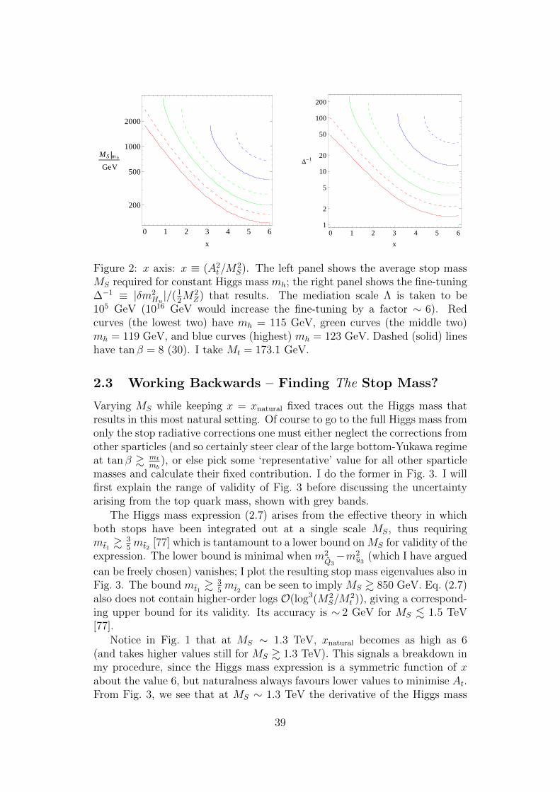
0 1 2 3 4 5 6

200

500

1000

2000

x

MS mh

GeV

0 1 2 3 4 5 61

2

5

10

20

50

100

200

x

D-1

Figure 2: x axis: x ≡ (A2t/M

2S). The left panel shows the average stop mass

MS required for constant Higgs mass mh; the right panel shows the fine-tuning∆−1 ≡ |δm2

Hu|/(1

2M2

Z) that results. The mediation scale Λ is taken to be105 GeV (1016 GeV would increase the fine-tuning by a factor ∼ 6). Redcurves (the lowest two) have mh = 115 GeV, green curves (the middle two)mh = 119 GeV, and blue curves (highest) mh = 123 GeV. Dashed (solid) lineshave tan β = 8 (30). I take Mt = 173.1 GeV.

2.3 Working Backwards – Finding The Stop Mass?

Varying MS while keeping x = xnatural fixed traces out the Higgs mass thatresults in this most natural setting. Of course to go to the full Higgs mass fromonly the stop radiative corrections one must either neglect the corrections fromother sparticles (and so certainly steer clear of the large bottom-Yukawa regimeat tan β & mt

mb), or else pick some ‘representative’ value for all other sparticle

masses and calculate their fixed contribution. I do the former in Fig. 3. I willfirst explain the range of validity of Fig. 3 before discussing the uncertaintyarising from the top quark mass, shown with grey bands.

The Higgs mass expression (2.7) arises from the effective theory in whichboth stops have been integrated out at a single scale MS, thus requiringmt1 &

35mt2 [77] which is tantamount to a lower bound on MS for validity of the

expression. The lower bound is minimal when m2Q3−m2

u3(which I have argued

can be freely chosen) vanishes; I plot the resulting stop mass eigenvalues also inFig. 3. The bound mt1 &

35mt2 can be seen to imply MS & 850 GeV. Eq. (2.7)

also does not contain higher-order logs O(log3(M2S/M

2t )), giving a correspond-

ing upper bound for its validity. Its accuracy is ∼ 2 GeV for MS . 1.5 TeV[77].

Notice in Fig. 1 that at MS ∼ 1.3 TeV, xnatural becomes as high as 6(and takes higher values still for MS & 1.3 TeV). This signals a breakdown inmy procedure, since the Higgs mass expression is a symmetric function of xabout the value 6, but naturalness always favours lower values to minimise At.From Fig. 3, we see that at MS ∼ 1.3 TeV the derivative of the Higgs mass

39

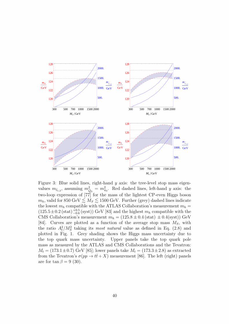
1000500 2000300 1500700

120

122

124

126

128

500.

1000.

1500.

2000.

Ms GeV

mh

GeV

mt

1,2

GeV

1000500 2000300 1500700

120

122

124

126

128

500.

1000.

1500.

2000.

Ms GeV

mh

GeV

mt

1,2

GeV

1000500 2000300 1500700

120

122

124

126

128

500.

1000.

1500.

2000.

Ms GeV

mh

GeV

mt

1,2

GeV

1000500 2000300 1500700

120

122

124

126

128

500.

1000.

1500.

2000.

Ms GeV

mh

GeV

mt

1,2

GeV

Figure 3: Blue solid lines, right-hand y axis: the tree-level stop mass eigen-values mt1,2 , assuming m2

Q3= m2

u3. Red dashed lines, left-hand y axis: the

two-loop expression of [77] for the mass of the lightest CP-even Higgs bosonmh, valid for 850 GeV .MS . 1500 GeV. Further (grey) dashed lines indicatethe lowest mh compatible with the ATLAS Collaboration’s measurement mh =(125.5±0.2 (stat)+0.5

−0.6 (syst)) GeV [83] and the highest mh compatible with theCMS Collaboration’s measurement mh = (125.8± 0.4 (stat) ± 0.4(syst)) GeV[84]. Curves are plotted as a function of the average stop mass MS, withthe ratio A2

t/M2S taking its most natural value as defined in Eq. (2.8) and

plotted in Fig. 1. Grey shading shows the Higgs mass uncertainty due tothe top quark mass uncertainty. Upper panels take the top quark polemass as measured by the ATLAS and CMS Collaborations and the Tevatron:Mt = (173.1±0.7) GeV [85]; lower panels take Mt = (173.3±2.8) as extractedfrom the Tevatron’s σ(pp→ tt+X) measurement [86]. The left (right) panelsare for tan β = 9 (30).

40

with respect to MS vanishes14, which is purely an artefact of the truncatedexpression. The Lagrange constrained optimisation, Eq. (2.5), is then solvedby the Higgs mass alone maximised with respect to both of its arguments,with the Lagrange multiplier λ vanishing i.e. the naturalness considerationdecouples. Hence the solution is pushed onto exactly maximal mixing. Evenhigher order terms in the Higgs mass expression would be needed to push thisbreakdown point out to higher stop masses.

The authors of [85], following a similar analysis to [87], take the top quarkmass measurement relevant for calculation of the (Standard Model) Higgs massto be a combined measurement of the pole mass from the ATLAS and CMSCollaborations and the Tevatron: Mt = (173.1±0.7) GeV. In [86] it was arguedthat direct experimental measurement of the top quark pole mass gives a the-oretically ill-defined quantity, and that a more theoretically rigorous approachis to extract the running mass from measurement of the top pair productioncross-section, and thence obtain Mt = (173.3 ± 2.8) GeV. I show both casesin Fig. 3; the choice of error in Mt has a striking effect on the Higgs massuncertainty.

An initial hope for this work was to see whether a given Higgs mass couldgive an indication of the average stop mass, using the principle of optimalnaturalness to reduce the function15

mh ≈ mh(MS, x) → mh(MS)|x=xnat(2.10)

The latter is shown in Fig. 3 with its uncertainty arising from the top quarkmass uncertainty ∆Mt; where it intersects with the observed Higgs mass, whichhas its own error ∆mh, we see which stop masses are possible. Fig. 3 showsthat even with the simplification of Eq. (2.10), the uncertainties ∆Mt and ∆mh

alone make any inference of MS from mh very difficult. This is compounded bya theoretical uncertainty in the calculation of mh, widely taken to be ∼3 GeV[88] (or perhaps larger still for heavy or highly non-degenerate stops), andthe smaller contributions from the particles besides the stops. The smallestMS compatible with the observed mh, found for large tan β and conservative∆Mt, can be read off as ∼350 GeV; however the stop quark mass eigenvaluesare then too split to trust a calculation based on integrating them both outat once (as discussed earlier). Fig. 3 also makes clear that even higher orderterms than the two-loop corrections to mh are necessary to constrain MS fromabove, as the monotonic increase of mh with MS needs to be captured. (Anupper limit on MS without naturalness is given in [18] – a few 108 GeV for splitSusy and unconstrained for high-scale Susy; MSSM-to-SM matching is neededto calculate mh with stops far beyond the weak scale.)

14Note that the derivative of interest is mh with respect to MS , with x held constant;in Fig. 3 the latter is not constant. However it is varying sufficiently slowly that whenwe instead hold it exactly constant, the relevant derivative still vanishes at the same pointMS ∼ 1.3 TeV.

15Necessarily for a choice of tanβ; large but less than mt

mb∼ 40 gives us a maximal Higgs

mass and without a fine-tuning penalty, which is clearly optimal.

41

I consider RG improvement to go beyond a leading log expression for δm2Hu

,but relegate this to Appendix B as the discussion is more involved thoughultimately gives the same xnatural.

2.4 Implications

This study being analytic throughout, it is complementary to the many numer-ical investigations of the Higgs in Susy performed recently, illustrating moreclearly the Higgs-stop-naturalness connection. I have shown that almost max-imal mixing, with x ≡ A2

t/M2S slightly lower than 6, is optimal; though I have

also shown that the distinction between this case and maximal mixing x = 6is academic. In other words to achieve a given Higgs mass mh, balancing Atand MS to optimise naturalness gives almost the same result as simply try-ing to minimise MS. (Note that maximal mixing is not ‘needed’ to achievemh ≈ 126 GeV, as has been reported for example in [89] – Fig. 6 of [58] forexample shows that MS = O(5 TeV) is sufficient with no mixing – it is merelya less tuned method of doing so.)

However conversely, even remaining in the MSSM, comparing how easilydifferent models accommodate a 126 GeV Higgs (a major focus of recent Susyphenomenology) based on how light the stops are is misleading. A maximal-mixing scenario will certainly have larger mh than a no-mixing scenario at thesame MS. But note that the reasoning of the previous paragraph applies to afixed mediation scale Λ. If the maximal-mixing scenario has much larger Λ thanthe no-mixing scenario – e.g. if we take the former to represent supergravityand the latter low-scale gauge-mediated Susy breaking (GMSB) – then it willbe more unnatural not only due to the large At but also due to large amountof RG running, i.e. the large logarithm in Eq. (2.3). Taking Λ = 1016 GeV and105 GeV as representative of these two cases, the former will have an unnaturalδm2

Huterm ∼25 times larger; the two should thus compare their Higgs masses

with GMSB having stops (roughly√

25 times) heavier than supergravity forsimilar fine-tuning, changing perhaps qualitatively the result of a comparisonat fixed MS, c.f. [57, 69]. The optimal situation in the MSSM is clearly (nearly)maximal mixing with low-scale mediation: [90] and [91] realised this with theintroduction of large At terms into GMSB via Higgs-messenger superpotentialcouplings.

Investigating whether minimal stop masses coincide with optimal natural-ness, as done here for the MSSM, is particularly important for extensions ofthe MSSM. Introducing a new particle which couples strongly to the Higgs, inorder to boost the latter’s mass without heavy stops, is naively good for nat-uralness. However pushing this new coupling as far as it will go can easily beimagined to introduce a new source of tuning somewhere in the theory (analo-gous to the effect of large At on δm2

Huconsidered here). Exactly this effect in

the Next-to-Minimal Supersymmetric Standard Model (NMSSM) was consid-ered in [92]: the stop masses and mixing were kept small, and the naturalnessimplications of NMSSM-specific contributions to mh calculated. These were

42

found to be a tuning of the lighter scalar’s couplings to hide it from currentcollider constraints, in the case where the 126 GeV Higgs is the second-lightestscalar; and worse tuning still when it is the lightest scalar, to undo the push-down effect of level-repulsion between mass eigenvalues. Nevertheless thesetunings are at the level of 1 part in 5, making the NMSSM more natural whencompared to the inescapable tuning of 1 part in ∼100 in the MSSM to obtainmh ≈ 126 GeV [54].

43

3 The Higgs In The NMSSM

This section is based on my work [93] done in collaboration with Daniel Al-bornoz Vasquez, Genevieve Belanger, Celine Bœhm, Jonathan Da Silva andPeter Richardson; the text has been mostly re-written.

3.1 Introducing The NMSSM

The NMSSM (see [94] for a review and original references) contains the samefield content as the MSSM – Table 2 – with the addition of a gauge-singletsuperfield S. The latter contains a neutral fermion – the singlino S, whichmixes with the four MSSM-like neutralinos to give χ0

i=1...5; together with aneutral scalar and pseudo-scalar, which mix with the doublet-like/MSSM-likeh and H to give Hi=1,2,3, and with the MSSM-like A to give A1,2, respectively.

A major motivation for this extension is to solve the µ-problem of theMSSM. From Eq.s (1.10) and (1.11) it is clear that |µ|2 cannot be consid-erably greater than the Higgs soft mass-squareds (particularly m2

Hu), or else

electroweak symmetry will not be broken. However this is precisely what wewould expect in the MSSM as µ is supersymmetric (appearing in the superpo-tential) and hence its natural scale is the cutoff of the supersymmetric theory,which we are imagining might be the GUT scale or beyond. To tie the size ofµ to the size as the soft terms one could appeal to the anthropic principle, butsince the latter may address the small size of the Standard Model Higgs masswithout Susy, a primary motivation is lost. Instead one can have an effectiveµ term arise as the VEV of a new superfield, which only acquires a VEV dueto Susy breaking; in the NMSSM that new superfield is the gauge singlet S.

Generally of course the explicit µ term is also present, and by introducingS there are two more dimensionful supersymmetric terms possible – a massand a tadpole for S – which also need to be suppressed well below valuescomparable to the cutoff scale in order to allow EWSB.

WNMSSM =WMSSM,Yukawas +WHiggs−only

with WHiggs−only = λSHuHd + µHuHd + χFS + 12µ′S2 + 1

3κS3 (3.1)

The three dimensionful supersymmetric terms – µHuHd, χFS and 12µ′S2 – can

be forbidden with a Z3 symmetry, giving a scale-less superpotential only con-taining terms with three superfields. If this discrete symmetry (or any other) isexact down to the electroweak scale where it is spontaneously broken, cosmo-logically unacceptable domain walls would exist between regions of space withdifferent charges under the symmetry – bubbles [95]. It is therefore desirable tosuppress such terms with only an approximate symmetry (see the discussionin [94]).

The Z3 symmetry forbidding dimensionful supersymmetric terms also for-bids three Susy-breaking terms: L/⊃− bHuHd + 1

2m′2SS

2 +χSS + c.c.. The soft

44

terms that are present and contribute to the Higgs potential at tree-level are

− Lsoft,Higgs = m2Hu|Hu|2 +m2

Hd|Hd|2 +m2

S|S|2

+ (λAλHuHdS + 13κAκS

3 + c.c.) (3.2)

The coefficients of these five terms, together with those of the two remainingZ3-symmetric terms inWHiggs−only (that is, λSHuHd and 1

3κS3) define the seven

parameters in the Z3-symmetric NMSSM Higgs sector: m2Hu

, m2Hd

, m2S, Aλ,

Aκ, λ and κ. The three scalar mass-squareds can be traded for the observedMZ , tan β, and the effective µ term µeff ≡ λ〈S〉.

The physical Higgs mass is boosted at tree-level, compared to the MSSM,by the coupling to the singlet: a purely doublet-like H1 has m2

H1,tree ≤M2

Z cos2 2β+λ2v2 sin2 2β with equality in the decoupling limit. Vanishing λ isthe MSSM case, for which mh plummets as tan β → 0; for λ = MZ/v ≈ 0.52,mh = MZ independent of tan β; and λ > 0.52 is when we start seeing a boostbeyond what is possible in the MSSM: see Fig. 4. There is however an up-per limit on the size of λ at the low scale in order to have it not encountera Landau pole before the GUT scale – this upper limit is ∼ 0.7 but becomesmuch smaller at low tan β. Pushing into the low-tan β large-λ region, which isdesirable for an enhanced tree-level mh, therefore pushes the viability of pertur-bation theory. According to [96, 54] minimal tuning is achieved for maximallynon-perturbative λ (namely λ ≈ 2), where a Landau pole is encountered andat the lowest scale permitted by precision measurements ∼10 TeV. This waschallenged in [97] where, with a slightly different measure of fine-tuning, λ ∼ 1was found to be preferred.

3.2 Scanning Parameter Space

In [93] my collaborators and I analysed the Higgs and collider phenomenologyof two scans of NMSSM parameter space which had been performed in [98,99, 100] and explored in a predominantly astrophysical context. Details ofhow the scans were set up can be found in the original works, however I willsummarise here.

• The key difference between the two scans was that the earlier one de-manded a lightest-neutralino mass mχ0

1< 15 GeV, motivated by hints of

a signal in direct detection experiments [101, 102]. Since these did notmaterialise into more concrete observation this requirement was droppedfor the second study, which contains points with arbitrary mχ0

1. In our

work [93] we analysed the two cases separately, as mχ01< 15 GeV requires

a delicate fine-tuning of parameters in order to be viable, and exhibitssome special features. The arbitrary mχ0

1case was extended with an

additional exploration of the λ > 0.5, tan β < 5 region in order to studyin greater detail well-mixed light Higgs bosons with large singlet com-ponent, which may enhance the signal strength (see the glossary) in theHiggs to diphoton channel – see Section 3.4.

45

60

70

80

90

100

110

120

1 2 3 4 5 6 7 8 9 10

mH

1, tr

ee

/ G

eV

tanβ

λ = 0 (MSSM)λ = MZ / v = 0.52

λ = 0.7

Figure 4: The maximum value (achieved in the decoupling limit) of the tree-level mass of a purely doublet-like H1 in the NMSSM: mh,tree =

√(M2

Z cos2 2β+λ2v2 sin2 2β). A singlet-doublet coupling of strength λ ≈ 0.7 is the maximumallowed by perturbativity / absence of Landau poles for a range of tan β,however as tan β approaches 1 a much smaller λ is required.

• A large number of independent ‘model’ parameters were defined at thelow scale, i.e. with no particular UV completion in mind. These param-eters were taken to be the gaugino masses M1, M2 and M3; Higgs sectorparameters µeff , tan β, λ, κ, Aλ and Aκ (as discussed in the previous sec-tion); flavour-blind soft masses for the left- and right-handed sleptons mL

and me; common soft masses for the squarks of the first and second gen-eration (Mq1,2) and third generation (Mq3), and a single non-zero trilinearcoupling, At. For the mχ0

1< 15 GeV study three further restrictions were

imposed: a common soft mass was taken for both ‘chiralities’ of sleptons(mL = me), squark masses were taken to be flavour blind (Mq3 = Mq1,2),and the gaugino mass-unification relation M2 = 1

3M3 was assumed. The

latter was taken to reduce the number of free parameters knowing thatthe gluino does not play an important role in dark matter observablesfor light neutralinos. For the later analysis without the mχ0

1< 15 GeV

requirement these three conditions were relaxed, increasing the param-eter space dimensionality by three. The spectrum and observables werecalculated from the model parameters using micrOMEGAs 2.4 [103] andNMSSMTools 2 [104, 105, 106].

• Some experimental constraints were applied as simple pass/fail criteria,while for others a likelihood was calculated, giving a goodness of fit forthe model for that particular observable. A total likelihood (as the prod-uct of all of the separate likelihoods) was calculated and used to help steerthe Markov Chain Monte Carlo’s parameter-space exploration towardsareas in better agreement with the full set of observables. Contributing

46

factors to this likelihood were:

– A comparison of the LSP relic density to the Wilkinson MicrowaveAnisotropy Probe (WMAP) observed value ΩWMAPh

2 = 0.1131 ±0.0034 [107], providing a constraint on the neutralino pair anni-hilation cross-section in the primordial Universe. The relic den-sity was calculated assuming Friedman-Robertson-Walker cosmol-ogy, standard thermodynamics and the freeze-out mechanism. Arelic density deficit Ω < ΩWMAP calls for another type of particle to(partially) solve the dark matter problem, or else a modification ofgravity (e.g. [108]).

– Dark matter direct detection limits from XENON100 [109], gammarays from dwarf spheroidal (dSph) galaxies probed by Fermi-LAT[110, 111] and the radio emission in the Milky Way and in galaxyclusters [112, 113].

– The anomalous magnetic moment of the muon: (g − 2)µ.

– Constraints included within NMSSMTools from b physics, and LEPand Tevatron Higgs and Susy searches (including invisible decaysof the Z).

– Theoretical constraints, namely the absence of Landau poles andunphysical global minima of the scalar potential.

In [93] we studied the effect of applying further constraints to these scans.LHC searches for Susy were considered, in the form of the ATLAS Collabora-tion’s 1.04 fb−1 jets+ /ET search which I implemented and validated in [114].For the reader unfamiliar with such searches, the points in this paragraphmay become clearer after the discussions in Section 7. As the standard toolfor the calculation of Next-to-Leading Order (NLO) cross-sections in Susy –Prospino[115, 116, 117, 118, 119] – is restricted to the MSSM, constraints werederived at Leading Order (LO) unlike in Section 7. Without the K-factor (seethe glossary), which is O(1− 3) in the MSSM, these constraints are expectedto be slightly conservative. To derive them, events (see the glossary) were gen-erated with Herwig++ 2.5.1 [120, 121] and analysed with RIVET 1.5.2 [122].These limits are capable of excluding first and second generation squarks lighterthan 0.6 − 1 TeV and gluinos lighter than ∼ 0.5 TeV; however they rely onlarge branching ratios of these particles into jets and a stable neutral particlesuch as a neutralino. In the NMSSM with a singlino-like neutralino LSP, thesquarks and gluinos cannot decay to this LSP directly but must do via anintermediate particle, frequently the second-lightest (MSSM-like) neutralino.As noted in [123] this reduces the acceptance (see the glossary) into jets+/ET

search channels, as the extra step reduces the /ET and may result in leptons16.

16Susy searches with leptons would then have greater sensitivity, but this typically doesnot compensate for the loss of sensitivity in the 0-lepton search [123]; at first glance astrange result since leptons are more striking objects over the quantum chromodynamics

47

q

q

χ0

2

χ0

2

A orH

A orH

χ0

1

χ0

1

bb

bb

qq

pmiss

T

Figure 5: The jets+/ET signal arising in the NMSSM with a singlino-like LSP,and a χ0

2 which is much lighter than the squarks and which decays to χ01 with

a Higgs (‘A or H’).

A third factor which I observed being of equal importance is that even if theintermediate state (between squark/gluino and LSP) decays into the LSP witha jet rather than a lepton, there will be greater alignment between the /pT andone of the jets, causing greater difficulty in meeting the angular separation trig-ger ∆φ(jet, /pT ). For the mχ0

1< 15 GeV scan, whenever the coloured sparticles

were light enough to be within reach of the LHC they were associated witha singlino-like χ0

1. The jets+ /ET search has highly reduced sensitivity for theaforementioned reasons and excluded very few of the points. For the arbitrarymχ0

1scan, however, the singlet sector particles were generally much heavier, so

that the LSP was not singlino-like. The MSSM-like q → qχ01 and g → qqχ0

1

decays then take place, resulting in the familiar limits mq & 0.6 − 1 TeV,mg & 0.5 TeV.

The observation of increased alignment between /pT and a jet prompted meto note in [93] the signal shown in Fig. 5. This arises in the case of a singlino-like χ0

1 (forcing squarks to decay instead via χ02) and a Higgsino-like χ0

2 whichis (a) able to decay to χ0

1 with a Higgs (the latter going to bb) and (b) muchlighter than the squarks (making it boosted). The result is a /pT vector whichis sandwiched in between two jets, each consisting of two b quarks. In [124](Section 8 of this thesis) I showed the relevance of this topology to simplerfinal states and many more classes of models, and how it can be exploited toreconstruct mass peaks.

The main constraint we were interested in investigating in [93] was com-patibility of the NMSSM with the first observation of the 126 GeV Higgs. Atthe time this had also been studied in [54, 61, 125, 126, 127] (and our pre-liminary results had appeared in [128]). Following the suggestion of [56] weconsidered 122 < mh/GeV < 128 as the favoured range, within experimentaland theoretical errors. Note that the observed Higgs h can correspond to H1,H2 or both at once (also in principle H3 is possible, though we did not find aviable example). As well as having the correct mass, a candidate for the ob-served signal must also have the correct signal strengths. These quantities are

(QCD) background, but when large /ET is replaced by modest +/ET and a modestly hardlepton, backgrounds with W bosons become relevant.

48

measured in the experiments, normalised to a Standard Model-like Higgs anddenoted by µ, as the factor by which the expected signal should be multipliedin order for the signal plus background to best agree with the observed events,as a function of mh (see my discussion of blue-band plots in Appendix C).

Proton collisions can produce a Higgs in different ways, however the mech-anism with the largest total cross-section (by a factor ∼10) for mh ∼ 126 GeVis the fusion of two gluons. If cuts (see the glossary) are imposed, they canhave different acceptances for the different production mechanisms and thuspreferentially select some more than others, possibly reducing the dominanceof gluon fusion. This is not the case for the cuts used in the three most sensitivechannels h→ γγ,WW,ZZ, and so for the signal strength in these channels agood approximation is to consider the normalised production cross-section asbeing given by the normalised coupling to gluons (squared):

σprod/σprod, SM ≈ g2hgg/g

2hgg,SM, (3.3)

RggXX ≡g2hgg BR(h→ XX)

g2hgg,SM BR(h→ XX)SM

, (3.4)

and we takeRggXX as the signal strength in theXX channel, XX = γγ,WW,ZZ.As a loose criterion for sufficient visibility to correspond to the observed sig-nal, I separated out points with Rggγγ ≥ 0.4 for 2σ agreement with the mostsignificant measurement – h→ γγ as seen by the ATLAS Collaboration.

To supplement the Higgs constraints hard-coded into NMSSMTools, I in-terfaced the latter to HiggsBounds [129, 130] for a further thorough check ofexisting Higgs-sector limits (see also Section 7.2). The code for doing this isavailable at [131].

3.3 Higgs Signals For mχ01< 15 GeV

Firstly we considered the broader case of χ01 as only a partial contributor

to the observed relic density: 10%ΩWMAPh2 < Ωχ0

1h2 ≤ ΩWMAPh

2 (with thelower bound admittedly somewhat arbitrary). In Fig. 6 I plot the distributionof masses and diphoton signal strengths for H2. In our scan H2 is most oftendoublet-like, i.e. with couplings like h in the MSSM, and thus values of mH2

extend roughly down to the LEP limit and up to 130 − 150 GeV. The fourcolours are explained in the caption; black points are good candidate points –at least one Higgs has mass ∈ [122, 128] GeV with Rggγγ ≥ 0.4. Fig. 6 showsthat this Higgs is almost always H2 in our scan, and for a handful of points itis H1 (visible as black points with mH2 /∈ [122, 128] GeV).

The (normalised) diphoton signal strength can be seen to extend to muchlower values than the Standard Model value of 1. This is chiefly because withmχ0

1< 15 GeV, at least one extra decay mode is open to the candidate Higgs

of mass ∼126 GeV: h → χ01χ

01. Furthermore, sufficiently efficient annihilation

of such light neutralinos for acceptable relic density is not found to be possiblewithout a resonant s-channel scalar A1 or pseudo-scalar H1 [98]. Hence either

49

Figure 6: Diphoton signal strength Rggγγ as a function of the mass of H2 inthe scan with mχ0

1< 15 GeV. Red points are ruled out either by jets+/ET

constraints (only three points) or by HiggsBounds 3.6.1; other colours passthese constraints. Green points have no scalar with mass ∈ [122, 128] GeV,blue points do have such a scalar (H1 and/or H2) but with Rggγγ < 0.4, andblack points have such a scalar with Rggγγ ≥ 0.4.

A1 or H1 has mass ∼2mχ01. 30 GeV, as shown in Fig. 7, and a Higgs-to-Higgs

decay is also open.

In Fig. 8 I plot only the (previously black) good candidate points, and showthe effect on the diphoton signal strength of competing beyond the StandardModel (BSM) decays h → χ0

1χ01, χ

01χ

02, A1A1, H1H1. One sees Rggγγ ≈ 1 −

BR(h → BSM), showing that the presence or absence of these decays is thedominant factor controlling signal strength. In Fig. 9 I show how the branchingratios for these decays are distributed amongst the good candidate points.

As an aside it is interesting to note that a light scalar or pseudo-scalar x,with reduced couplings to standard model particles (to explain current non-observation) but into which the Higgs can decay, is seen here in the NMSSMbut is a widely motivated phenomenon. For example a symmetry of the Higgspotential explicitly broken by a small term in the Lagrangian will give a lightdegree of freedom strongly coupled to the physical Higgs (see the more detaileddiscussion in [132]). The decay of x following h→ 2x is model dependent, andmany possibilities have been considered. One example is a decay to gluonswhich suffers from a huge QCD background [133], however a boosted h→ 2x→4g fat jet has characteristic (and intuitive) jet substructure [134, 135]: the twohardest subjets are likely to have small masses (equal to mx), they are likelyto have similar masses, and they are likely to be much harder than the thirdhardest subjet. Other possible decays include those to taus [136, 137], tausand muons [132], charm quarks [138], and generic combinations of hadronicand missing energy [139].

A lighter Higgs could of course be produced directly, as well as via the decay

50

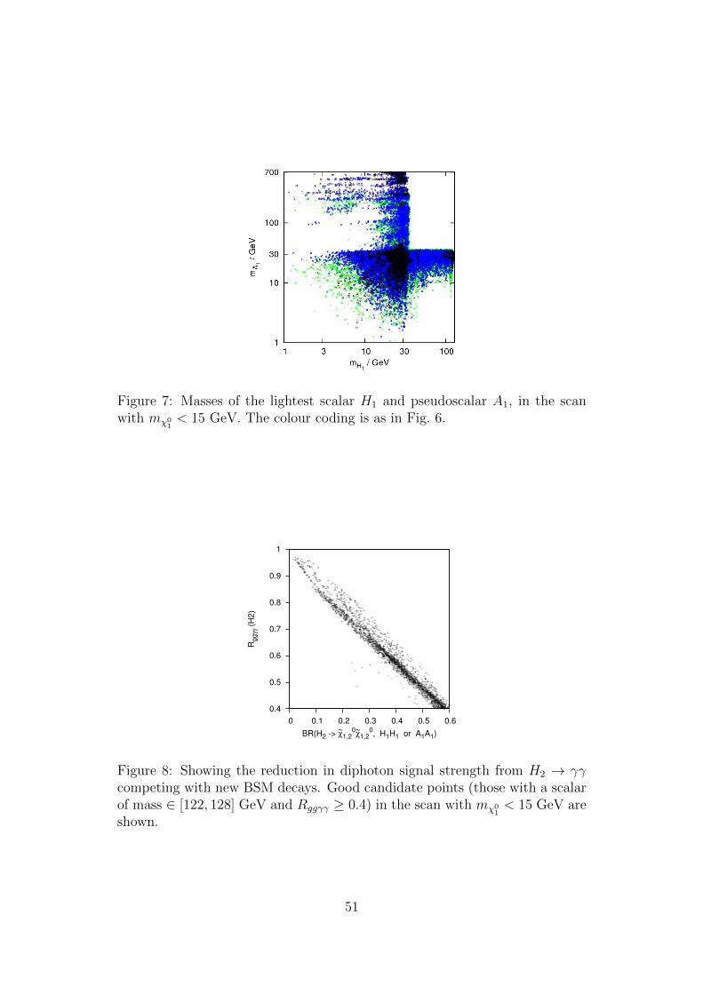
Figure 7: Masses of the lightest scalar H1 and pseudoscalar A1, in the scanwith mχ0

1< 15 GeV. The colour coding is as in Fig. 6.

0.4

0.5

0.6

0.7

0.8

0.9

1

0 0.1 0.2 0.3 0.4 0.5 0.6

Rgg

γγ (

H2

)

BR(H2 -> χ~1,20χ~

1,20, H1H1 or A1A1)

Figure 8: Showing the reduction in diphoton signal strength from H2 → γγcompeting with new BSM decays. Good candidate points (those with a scalarof mass ∈ [122, 128] GeV and Rggγγ ≥ 0.4) in the scan with mχ0

1< 15 GeV are

shown.

51

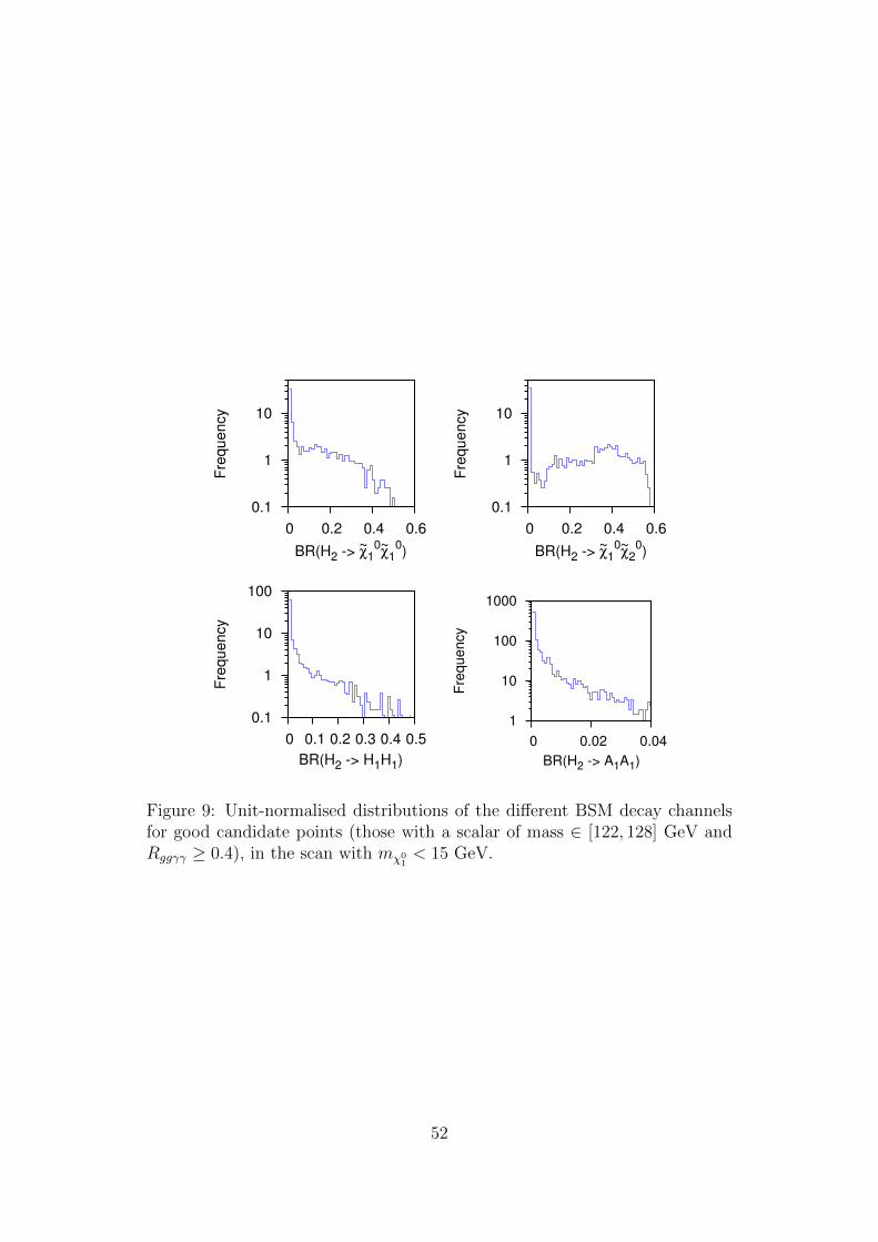
0.1

1

10

0 0.2 0.4 0.6

Fre

qu

en

cy

BR(H2 -> χ~10χ~

10)

0.1

1

10

0 0.2 0.4 0.6

Fre

qu

en

cy

BR(H2 -> χ~10χ~

20)

0.1

1

10

100

0 0.1 0.2 0.3 0.4 0.5

Fre

qu

en

cy

BR(H2 -> H1H1)

1

10

100

1000

0 0.02 0.04

Fre

qu

en

cy

BR(H2 -> A1A1)

Figure 9: Unit-normalised distributions of the different BSM decay channelsfor good candidate points (those with a scalar of mass ∈ [122, 128] GeV andRggγγ ≥ 0.4), in the scan with mχ0

1< 15 GeV.

52

of the 126 GeV Higgs. The substantial singlet component necessary to escapeexisting constraints suppresses the coupling to Standard Model particles. Inthe NMSSM (and other type II two-Higgs-doublet models [140]) couplings toleptons and down-type quarks are enhanced by tan β, possibly enhancing theassociated production of the lighter Higgs with a b quark, followed by a decayto 2τ . In this scan however we found an H1bb coupling equal to the StandardModel value at most.

Finally we checked the effect of requiring that points in the scan have arelic density within 1σ of the WMAP observed value (rather than merely notexceeding it). This depleted the density of points surviving all constraintsapparently uniformly, without causing any further noticeable correlations inthe Higgs signals.

3.4 Higgs Signals For Arbitrary mχ01

The condition mχ01< 15 GeV required a fine tuning of parameters to be

viable, as I have mentioned, and forced the lightest scalar or pseudo-scalarto have mass ∼2mχ0

1(and thus necessarily be singlet-like). The scan without

this condition typically gave rise to χ01 considerably heavier than 15 GeV,

which can annihilate efficiently through exchange of a Z or light slepton, andtherefore do not require (part of) the singlet sector to be light for acceptablerelic density. Indeed in this scan the singlet sector is generally heavier thanin the previous one, and H1 rather than H2 is usually the candidate withmass ∈ [122, 128] GeV.

Again we started by considering χ01 as simply a contributor to the observed

relic density, now without a lower bound: Ωχ01h2 ≤ ΩWMAPh

2. In Fig. 10 Ishow plots made by my collaborator Daniel Albornoz Vasquez illustrating thedistribution of diphoton signal with mass, for all such points. Constraintsfrom HiggsBounds 3.6.1 have been checked, those from jets+/ET searcheshave not (yet). Very strong enhancement of the H1 diphoton signal strengthis seen, though mostly for masses below ∼126 GeV. For both H1 and H2 amodest enhancement O(2) is seen in the favoured mass range. This is possiblewhen the singlet scalar eigenstate is close in mass to the lightest doublet-likescalar, such that the singlet nature of the former partially mixes into the latter,suppressing the largest Higgs decay width Γh→bb and permitting an increasedbranching ratio to two photons as explained in [141, 125].

Such a mechanism for enhancing the diphoton signal strength is weaklymotivated by (statistically insignificant) excesses observed particularly by theATLAS Collaboration – currently at the level 2.4σ [142, 143] – and previouslyby the CMS Collaboration (no more – [144]). Let us understand it in greaterdetail. With the matrix Sig relating the gauge eigenstate scalars g = H0

u, H0d , S

53

Figure 10: Diphoton signal strength Rggγγ as a function of the mass of H1

(left panel) and of H2 (right panel), in the scan with arbitrary mχ01. In the

left panel most points are on top of one another at high mass and high Rggγγ.The colour coding is as in Fig. 6 except jets+/ET constraints are not checked.Plots by Daniel Albornoz Vasquez.

to the mass eigenstates Hi=1,2,3, the modified couplings are at tree-level:

gHibbgHibb, SM

=Sid

cos β, (3.5)

gHiV VgHiV V, SM

= Sid cos β + Siu sin β (3.6)

The latter is relevant because the decay of a Higgs to two (massless) photons ispurely loop induced, dominantly through a W loop, thus strongly correlatingthe coupling to γγ with the coupling to WW . If the coupling to WW isdecreased exactly in line with the coupling to bb, the diphoton signal strengthwill remain Standard Model-like (unless new light charged particles enhancethe coupling of the Higgs to photons). Comparing Eq.s (3.5) and (3.6) wesee that the diphoton signal strength is not enhanced when cos β = 1, whichmeans the bottom-type Yukawas are exactly Standard Model-like; mixing asinglet with the doublet state then depletes all couplings uniformly, as wouldhappen in the Standard Model, preventing modification of branching ratios.We see that non-trivial mixing between the two doublet states (Hu and Hd) isrequired in addition to mixing with the singlet.

As for the scan with mχ01< 15 GeV, we checked the effect of requiring χ0

1 tomake up all of the WMAP observed relic density (within 1σ). This eliminatedall of the points in our scan where the diphoton signal strength was appreciablyenhanced, 1 . Rggγγ . 2 (leaving a new maximum Rggγγ of 1.06). These pointshad a light singlet scalar, m2

S = (κµeff/λ)(Aκ+4κµeff/λ) [145, 94], by virtue ofa small µeff . 200 GeV. This leads to some amount of Higgsino component inχ0

1, allowing it to annihilate more efficiently and reducing the relic density (inour case always below ΩWMAPh

2). Nevertheless in [63] an enhanced diphotonrate was found in the NMSSM with a WMAP-compatible relic density; note

54

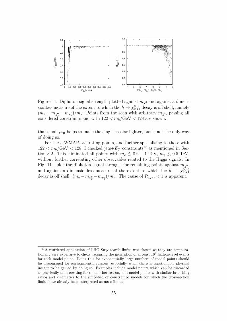
0.4

0.5

0.6

0.7

0.8

0.9

1

1.1

0 50 100 150 200 250 300 350 400 450

Rgg

γγ (

H1

)

mχ1

0 / GeV

0.4

0.5

0.6

0.7

0.8

0.9

1

1.1

-7 -6 -5 -4 -3 -2 -1 0

Rg

gγγ (

H1)

(mH1 - m

χ20 - m

χ10) / mH1

Figure 11: Diphoton signal strength plotted against mχ01

and against a dimen-

sionless measure of the extent to which the h→ χ02χ

01 decay is off shell, namely

(mh −mχ02−mχ0

1)/mh. Points from the scan with arbitrary mχ0

1, passing all

considered constraints and with 122 < mh/GeV < 128 are shown.

that small µeff helps to make the singlet scalar lighter, but is not the only wayof doing so.

For these WMAP-saturating points, and further specialising to those with122 < mh/GeV < 128, I checked jets+ /ET constraints17 as mentioned in Sec-tion 3.2. This eliminated all points with mq . 0.6 − 1 TeV, mg . 0.5 TeV,without further correlating other observables related to the Higgs signals. InFig. 11 I plot the diphoton signal strength for remaining points against mχ0

1,

and against a dimensionless measure of the extent to which the h → χ02χ

01

decay is off shell: (mh−mχ02−mχ0

1)/mh. The cause of Rggγγ < 1 is apparent.

17A restricted application of LHC Susy search limits was chosen as they are computa-tionally very expensive to check, requiring the generation of at least 104 hadron-level eventsfor each model point. Doing this for exponentially large numbers of model points shouldbe discouraged for environmental reasons, especially when there is questionable physicalinsight to be gained by doing so. Examples include model points which can be discardedas physically uninteresting for some other reason, and model points with similar branchingratios and kinematics to the simplified or constrained models for which the cross-sectionlimits have already been interpreted as mass limits.

55

Part III

Gauge-Mediated Susy Breaking

4 Introduction

As mentioned in Section 1.3, Susy breaking must occur in a hidden sectorand be mediated to the visible sector (containing the MSSM), with the threemain candidates for the mediator being gravitational interactions, extra di-mensions, and gauge interactions. In this part of the thesis I will discuss somephenomenological aspects of the last of these cases – gauge-mediated Susybreaking (GMSB).

4.1 R Symmetry And Susy Breaking

One of the relations of the Susy algebra is that the Hamiltonian is a positivesemi-definite sum of the fermionic generators. This means that, for a Susytheory, the vacuum |0〉 has unbroken Susy if and only if it has vanishing en-ergy; Susy is broken if and only if the vacuum energy is strictly greater thanzero. To describe our universe with Susy (which is necessarily broken) we thenmust ensure either that the RHS of Eq. (1.6) is greater than zero (F -termbreaking) or that the RHS of Eq. (1.7) is greater than zero (D-term breaking).Phenomenological problems with the latter have concentrated most efforts onthe former, with non-vanishing F -terms widely considered to be necessary (notjust sufficient).

R symmetry is a symmetry of the Lagrangian but not the superpotential:it is the continuous symmetry

θ, dθ, W (Φ), L → eiαθ, e−iαdθ, e2iαW (Φ), L (4.1)

Under this symmetry the superpotential has charge 2: we write R(W ) = 2.In [146] a deep connection between R symmetry and dynamical F -term Susybreaking was established for generic, calculable theories. Dynamical Susybreaking models are those in which none of the mass scales associated withSusy breaking are put in by hand – all are generated by dimensional trans-mutation, being of the form MP e

−a/g2 , with a = O(4π2). Calculable theoriesare those with a limit in which (asymptotically free) gauge dynamics can beintegrated out at some scale, leaving an effective theory with only chiral super-fields and no gauge fields (or gauge fields which do not couple to the remaininglight chiral fields). These chiral superfields Φi=1...N can then be charged underglobal symmetries, and there are exactly three possibilities.

• There are no global symmetries. The superpotential W is a functionof N variables; the vanishing of the RHS of Eq. (1.6) amounts to Nconstraints for the existence of a supersymmetric vacuum.

56

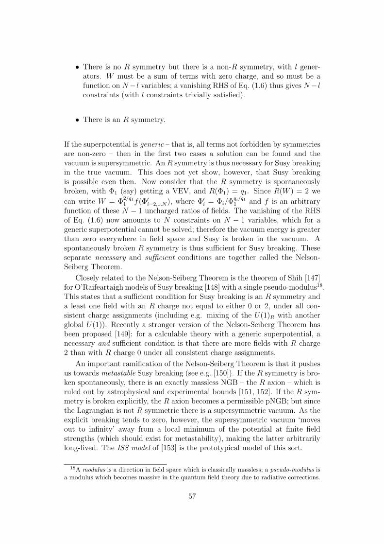
• There is no R symmetry but there is a non-R symmetry, with l gener-ators. W must be a sum of terms with zero charge, and so must be afunction on N− l variables; a vanishing RHS of Eq. (1.6) thus gives N− lconstraints (with l constraints trivially satisfied).

• There is an R symmetry.

If the superpotential is generic – that is, all terms not forbidden by symmetriesare non-zero – then in the first two cases a solution can be found and thevacuum is supersymmetric. AnR symmetry is thus necessary for Susy breakingin the true vacuum. This does not yet show, however, that Susy breakingis possible even then. Now consider that the R symmetry is spontaneouslybroken, with Φ1 (say) getting a VEV, and R(Φ1) = q1. Since R(W ) = 2 we

can write W = Φ2/q11 f(Φ′i=2,...N), where Φ′i = Φi/Φ

qi/q11 and f is an arbitrary

function of these N − 1 uncharged ratios of fields. The vanishing of the RHSof Eq. (1.6) now amounts to N constraints on N − 1 variables, which for ageneric superpotential cannot be solved; therefore the vacuum energy is greaterthan zero everywhere in field space and Susy is broken in the vacuum. Aspontaneously broken R symmetry is thus sufficient for Susy breaking. Theseseparate necessary and sufficient conditions are together called the Nelson-Seiberg Theorem.

Closely related to the Nelson-Seiberg Theorem is the theorem of Shih [147]for O’Raifeartaigh models of Susy breaking [148] with a single pseudo-modulus18.This states that a sufficient condition for Susy breaking is an R symmetry anda least one field with an R charge not equal to either 0 or 2, under all con-sistent charge assignments (including e.g. mixing of the U(1)R with anotherglobal U(1)). Recently a stronger version of the Nelson-Seiberg Theorem hasbeen proposed [149]: for a calculable theory with a generic superpotential, anecessary and sufficient condition is that there are more fields with R charge2 than with R charge 0 under all consistent charge assignments.

An important ramification of the Nelson-Seiberg Theorem is that it pushesus towards metastable Susy breaking (see e.g. [150]). If the R symmetry is bro-ken spontaneously, there is an exactly massless NGB – the R axion – which isruled out by astrophysical and experimental bounds [151, 152]. If the R sym-metry is broken explicitly, the R axion becomes a permissible pNGB; but sincethe Lagrangian is not R symmetric there is a supersymmetric vacuum. As theexplicit breaking tends to zero, however, the supersymmetric vacuum ‘movesout to infinity’ away from a local minimum of the potential at finite fieldstrengths (which should exist for metastability), making the latter arbitrarilylong-lived. The ISS model of [153] is the prototypical model of this sort.

18A modulus is a direction in field space which is classically massless; a pseudo-modulus isa modulus which becomes massive in the quantum field theory due to radiative corrections.

57

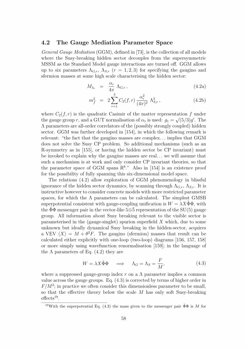
4.2 The Gauge Mediation Parameter Space

General Gauge Mediation (GGM), defined in [73], is the collection of all modelswhere the Susy-breaking hidden sector decouples from the supersymmetricMSSM as the Standard Model gauge interactions are turned off. GGM allowsup to six parameters ΛG,r, ΛS,r (r = 1, 2, 3) for specifying the gaugino andsfermion masses at some high scale characterising the hidden sector:

Mλr =αr4π

ΛG,r , (4.2a)

m2f

= 23∑r=1

C2(f, r)α2r

(4π)2Λ2S,r , (4.2b)

where C2(f, r) is the quadratic Casimir of the matter representation f underthe gauge group r, and a GUT normalisation of α1 is used: g1 =

√(5/3)g′. The

Λ parameters are all-order correlators of the (possibly strongly coupled) hiddensector. GGM was further developed in [154], in which the following remark isrelevant: “the fact that the gaugino masses are complex. . . implies that GGMdoes not solve the Susy CP problem. So additional mechanisms (such as anR-symmetry as in [155], or having the hidden sector be CP invariant) mustbe invoked to explain why the gaugino masses are real. . . we will assume thatsuch a mechanism is at work and only consider CP invariant theories, so thatthe parameter space of GGM spans R6.” Also in [154] is an existence prooffor the possibility of fully spanning this six-dimensional model space.

The relations (4.2) allow exploration of GGM phenomenology in blissfulignorance of the hidden sector dynamics, by scanning through ΛG,r, ΛS,r. It isinstructive however to consider concrete models with more restricted parameterspaces, for which the Λ parameters can be calculated. The simplest GMSBsuperpotential consistent with gauge-coupling unification is W = λXΦΦ, withthe ΦΦ messenger pair in the vector-like 5⊕5 representation of the SU(5) gaugegroup. All information about Susy breaking relevant to the visible sector isparameterised in the (gauge-singlet) spurion superfield X which, due to someunknown but ideally dynamical Susy breaking in the hidden-sector, acquiresa VEV 〈X〉 = M + θ2F . The gaugino (sfermion) masses that result can becalculated either explicitly with one-loop (two-loop) diagrams [156, 157, 158]or more simply using wavefunction renormalisation [159]; in the language ofthe Λ parameters of Eq. (4.2) they are

W = λXΦΦ =⇒ ΛG = ΛS =F

M, (4.3)

where a suppressed gauge-group index r on a Λ parameter implies a commonvalue across the gauge groups. Eq. (4.3) is corrected by terms of higher order inF/M2; in practice we often consider this dimensionless parameter to be small,so that the effective theory below the scale M has only soft Susy-breakingeffects19.

19With the superpotential Eq. (4.3) the mass given to the messenger pair ΦΦ is M for

58

The simple superpotential (4.3) has all six Λ parameters equal; their split-ting and independency comes from more general superpotentials. I will demon-strate this with just the fundamental representation of SU(5). Only up to fourindependent scales will be obtained: we always have ΛG,1 = 3

5ΛG,2 + 2

5ΛG,3 and

Λ2S,1 = 3

5Λ2S,2 + 2

5Λ2S,3 according to the relative hypercharges of the doublet l

and triplet q components of the SU(5) fundamental when decomposed20 ontoSU(3)× SU(2)× U(1).

As discussed in many places, such as [160, 161, 155, 162, 163] (this list isnot selective), one can generalise (4.3) with (a) multiple 5⊕ 5 messengers, (b)multiple spurions (or equivalently supersymmetric messenger mass terms), and(c) doublet-triplet splitting, i.e. independent Yukawa couplings for the doubletl and triplet q components of the 5. I summarise these 2× 2× 2 possibilities– corresponding to using or not using each of these three generalisations – inTables 3 and 4. The resulting soft terms follow from (4.3) with no furthercomputation:

• Multiple messengers. Each messenger appears in the one-loop gauginomass diagrams and the two-loop sfermion mass-squared diagrams, andso contributes additively to ΛG and Λ2

S. Therefore generalising Φ →Φi=1...N , with the Yukawa coupling λ becoming a matrix in messengerflavour space λij, has the effect

ΛG = ΛS =F

M

Φ→Φi=1...N−−−−−−−→ ΛG =N∑i=1

F

M, Λ2

S =N∑i=1

(F

M

)2

, (4.4)

provided we can diagonalise λij giving a basis in which the messengersare independent (more in this later).

• Multiple spurions. In Eq. (4.3), note that F/M is really λF/λM , sincethese dimensionful parameters only occur in conjunction with the Yukawacouping in the superpotential. Thus generalising to multiple spurions,λX → λaXa, replaces λF/λM by λaFa/λ

bMb in the soft masses. UnlessFa/Ma (no sum over a) is independent of a, the Yukawa coupling nolonger cancels in this ratio.

• Doublet-triplet splitting. Even if the Yukawa couplings of l and q tothe spurion are equal at the GUT scale, as would be required by gauge

the fermion and√

(M2±F ) for the two scalar degrees of freedom; note that this symmetricSusy breaking obeys Eq. (1.9) as it is a tree-level effect. Thus F < M2 is necessary to avoidtachyonic messengers, and F M2 avoids a hard Susy breaking theory where one messengerscalar m2

φ2= F +M2 has been integrated out but the other m2

φ1= F −M2 has not. Susy

broken only softly is necessary for a wavefunction renormalisation calculation [159].20In [154] it is shown that decomposing the total messenger sector into separate irreps with

respect to the Standard Model SU(3)×SU(2)×U(1), each irrep contributes additively to ΛG,rand Λ2

S,r, in proportion to its Dynkin index with respect to gauge group r. Contributinglinearly to ΛG,r but in quadrature to ΛS,r means a single irrep can result in up to two freeparameters; six independent ΛG,r,ΛS,r therefore requires at least three different irreps, forexample as in the 10 representation of SU(5). The fundamental has only two: q and l.

59

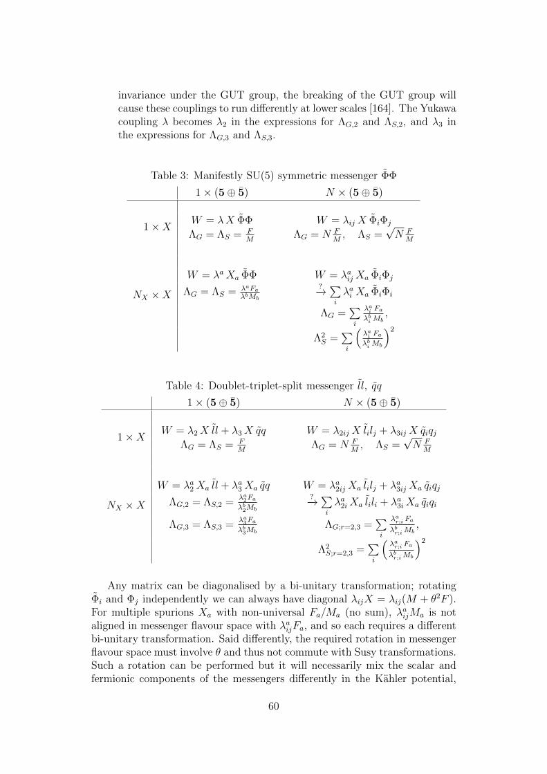
invariance under the GUT group, the breaking of the GUT group willcause these couplings to run differently at lower scales [164]. The Yukawacoupling λ becomes λ2 in the expressions for ΛG,2 and ΛS,2, and λ3 inthe expressions for ΛG,3 and ΛS,3.

Table 3: Manifestly SU(5) symmetric messenger ΦΦ

1× (5⊕ 5) N × (5⊕ 5)

1×X W = λX ΦΦ W = λij X ΦiΦj

ΛG = ΛS = FM

ΛG = N FM, ΛS =

√N F

M

NX ×X

W = λaXa ΦΦ W = λaij Xa ΦiΦj

ΛG = ΛS = λaFaλbMb

?−→∑i

λai Xa ΦiΦi

ΛG =∑i

λai Faλbi Mb

,

Λ2S =

∑i

(λai Faλbi Mb

)2

Table 4: Doublet-triplet-split messenger ll, qq

1× (5⊕ 5) N × (5⊕ 5)

1×X W = λ2X ll + λ3X qq W = λ2ij X lilj + λ3ij X qiqjΛG = ΛS = F

MΛG = N F

M, ΛS =

√N F

M

NX ×X

W = λa2 Xa ll + λa3 Xa qq W = λa2ij Xa lilj + λa3ij Xa qiqj

ΛG,2 = ΛS,2 =λa2Faλb2Mb

?−→∑i

λa2iXa lili + λa3iXa qiqi

ΛG,3 = ΛS,3 =λa3Faλb3Mb

ΛG;r=2,3 =∑i

λar;i Fa

λbr;iMb,

Λ2S;r=2,3 =

∑i

(λar;i Fa

λbr;iMb

)2

Any matrix can be diagonalised by a bi-unitary transformation; rotatingΦi and Φj independently we can always have diagonal λijX = λij(M + θ2F ).For multiple spurions Xa with non-universal Fa/Ma (no sum), λaijMa is notaligned in messenger flavour space with λaijFa, and so each requires a differentbi-unitary transformation. Said differently, the required rotation in messengerflavour space must involve θ and thus not commute with Susy transformations.Such a rotation can be performed but it will necessarily mix the scalar andfermionic components of the messengers differently in the Kahler potential,

60

and so one cannot integrate out each messenger separately21. This encouragesrestriction of the couplings λaij to diagonal form λai , in which case the simplelogic of the multiple messenger and multiple spurion bullet points precedingthis paragraph suffices to calculate the tricky case of multiple messengers andmultiple spurions.

Restriction to a diagonal messenger-spurion coupling is also necessary ingeneral, as noted in [162], to suppress potentially tachyonic hypercharge D-term contributions to sfermion masses. This is because a diagonal form ensuresthe existence of a messenger parity, defined in [160], where the messenger sectoris unchanged at tree level by Φi, Φi, V → Φi,Φi,−V (with V a gauge field).This parity forbids the troublesome hypercharge term. It is an approximatesymmetry only, necessarily broken by the visible sector couplings with thegauge fields, but this is enough to make the hypercharge term arise safely atthree or more loops instead of at one loop.

A different approach to calculating the soft terms for multiple messengersand spurions is taken in [155], which I will summarise below. One can rotatein the basis of spurions to give just one spurion that has an F -term, plus asupersymmetric mass matrix. Explicitly:

λaijXa = λaij(Ma + Fa θ2)

= (FaF1

λaij) (M1 + F1 θ2) + λaij(Ma −

FaF1

M1)

≡ λijX +mij

(4.5)

The explicit spurion-relabelling symmetry of the LHS is implicit in the RHSdue to a freedom to shift an arbitrary amount of the supersymmetric part ofthe spurion into the supersymmetric mass matrix:

λijM +mij = λij(M +M ′) + (mij − λijM ′). (4.6)

In the spurion basis defined by the rotation in Eq. (4.5), the authors of [155]assume a non-trivial R symmetry (i.e. R(X) 6= 0). This uniquely specifies thesplitting in Eq. (4.6), and picks out one spurion from amongst theXa as unique,since the charged and uncharged terms cannot mix; in this way the spurionre-labelling symmetry is seen to disappear from both the LHS and RHS ofEq. (4.5). (Note that if the R symmetry existed in the pre-rotation basis Xa,is might prevent rotation to the single-spurion form; an alternative to the ideaof rotation is of course a set up where there genuinely is just one spurion andsupersymmetric masses for the messengers.) For any λij and mij consistentwith the R symmetry (which enforces λij = 0 if mij 6= 0 and mij = 0 if λij 6= 0)the soft masses are then calculated as

ΛG = F ∂X log det(λijX +mij) |X=M =nF

M

with n =1

R(X)

N∑i=1

(2−R(Φi)−R(Φi))),(4.7a)

21Thanks to Alberto Mariotti for pointing this out.

61

Λ2S =

1

2|F |2 ∂2

∂X∂X∗

N∑i=1

(log |Mi|2

)2 |X=M (4.7b)

where Mi is the ith eigenvalue of Mij = λijX + mij. I add to Eq. (4.7b)only the comment that it is necessary for the interest of the setup that thediagonalisation of Mij does not respect the R symmetry. Otherwise, eacheigenvector Mi is a state of definite R charge, with an eigenvalue which iseither a coupling to the spurion or a supersymmetric mass; there are n of theformer and N − n of the latter kind of eigenvector. Eq. (4.7b) then evaluates

trivially to Λ2S = n

(FM

)2here as it must, matching ΛG = n F

Mto give nothing

but minimal GMSB with n messengers and one-spurion.For doublet-triplet split EOGM, independent ΛS,2 and ΛS,3 are found:

Eq. (4.7b) with Mi replaced by M2i and M3i respectively. ΛG,2 and ΛG,3

however remain constrained to be equal based on the assumption of the dou-blets’ R charges matching those of the triplets – they thus share a value forthe quantity n in (4.7a).

62

5 The Role Of The Messenger Scale, Sum Rules

And RG Invariants

This section is based on my works [165, 166] done in collaboration with JorgJackel and Valya Khoze; the text has been mostly re-written. Unlike thoseworks, here I use a GUT normalisation for the U(1) gauge coupling: g1 =√

(5/3)g′.

The GGM relations for the soft masses, Eq. (4.2), hold at some scale charac-terising the hidden sector. For models with a single (or several degenerate) ex-plicit messenger(s) of supersymmetric mass Mmess, coupled to a Susy-breakingF -term with F M2

mess, that scale is unambiguously Mmess: the scale atwhich all messenger degrees of freedom are integrated out. Consider holdingall high-scale parameters constant, but changing the scale Mmess at which theyset the soft masses. Since this changes the amount of running required to reachthe low scale, and all MSSM soft-mass beta functions are non-zero, then triv-ially the low-scale spectrum will change. From this point of view, Mmess is anadditional parameter impacting upon the low-scale GGM spectrum togetherwith the six Λ parameters.

Let us ask a more subtle question instead. If varying Mmess with constant Λparameters changes the low-scale spectrum, can this effect be entirely absorbedinto appropriately varying Λ parameters? If this were the case, Mmess wouldmerely parameterise a one-dimensional family of models, Λ(Mmess), with iden-tical low-scale spectra (neglecting the precise value of the sub-GeV gravitino).The answer to this question lies in sum rules and RG invariants (RGIs).

In GGM, the five sfermion soft masses (set in a flavour-blind manner) aregiven in terms of three parameters, ΛS;r=1,2,3, and thus there are two sumrules [73], exact at Mmess, which can be expressed as

Tr[Y m2] = 0, (5.1)

Tr[(B − L)m2] = 0 (5.2)

After running to the low scale, these are expected to hold for the first twogenerations but not the third, as they are de-tuned under RG evolution onlyby the Yukawas [73]. Let me say this a little differently. Setting the Yukawas tozero, the running of the sfermion soft masses depends only on the three gauginomasses; there are thus two linear combinations of sfermion mass-squared betafunctions (which are always the same in the MSSM) that vanish. In GGM, thelinear combinations of beta functions which vanish are the same as the linearcombinations of mass-squareds which vanish at Mmess, hence the preservationof the sum rules.

In [165] I calculated the values of the sum rules at low scale resulting frommodels of GGM (allowing for non-zero b(Mmess)) with their spectra calculatedusing SOFTSUSY 3.1.6 [167] supplemented with GGM boundary conditions. I

63

found them to hold to O(1%) for the first two generations and for the third-generation hypercharge sum rule; only the third-generation B − L sum rulewas broken strongly, by ∼ 10− 60% over the parameter space investigated.

The goodness of the first two generation sum rules at lower scales allowsfor the meaningful definition of Λ parameters which run, as opposed to beingdefined at the high-scale only – five running mass-squareds continue to bedescribed by three running parameters – ΛS,r(Q) at a scale Q. These aredefined up to arbitrary additions of the two vanishing sum rules; an intuitivechoice can be arrived at in the following way. Amongst the one-loop RGIsof the MSSM (setting the Yukawas of the first two generations to zero) listedin [168] are the six shown in Table 5.

RGI Definition GGM high-scale value

IBr Mr/g2r

ΛG,r16π2

IMr M2r +

∑f D(f , r)m2

f ,1

(αr(Mmess)

4π

)2 (Λ2G,r + κrΛ

2S,r

)Table 5: Six one-loop RGIs of the MSSM, setting the Yukawas of the first twogenerations to zero, with r = 1, 2, 3 denoting a gauge group, and m2

f ,1a first-

generation sfermion mass-squared, taken from [168]. Their values in GGM at ascale Mmess are shown. D(f , r) and κr are numerical coefficients whose values(suppressed here for clarity) can be found in that reference.

The first three of these, IBr , show that the parameters ΛG,r are themselvesRGIs; they can therefore trivially be defined at lower scales by ΛG,r(Q) = ΛG,r.Then since the IMr are constant, taking the expressions for their values in GGMat Mmess but allowing the αr to run defines implicitly how ΛS,r(Q) must runto keep IMr constant. In other words:

IMr =

(αr(Q)

4π

)2 (Λ2G,r + κrΛ

2S,r(Q)

)(5.3)

An example of how the ΛS,r(Q) run is shown in Fig. 12.

Where has defining running Λ parameters got us? Consider a taking a spe-cific GGM model defined by ΛS,r,ΛG,r and Mmess, and calculating the runningof ΛS,r,ΛG,r down to a lower scale Q. Now define another GGM model whoseparameters are Mmess equal to that scale Q, and ΛS,r,ΛG,r equal to the run-ning values just calculated. By construction, these two models will have thesame running Λ parameters at all scales below the lower messenger mass, andthus be indistinguishable; the effect of larger Mmess / more RG running can beabsorbed into the Λ parameters (I am still neglecting Yukawa couplings – thisstatement will shortly be revised). I illustrate this with the cartoon Fig. 13.Similarly Fig. 12 can be reinterpreted, instead of showing the running ΛS,r(Q)

64

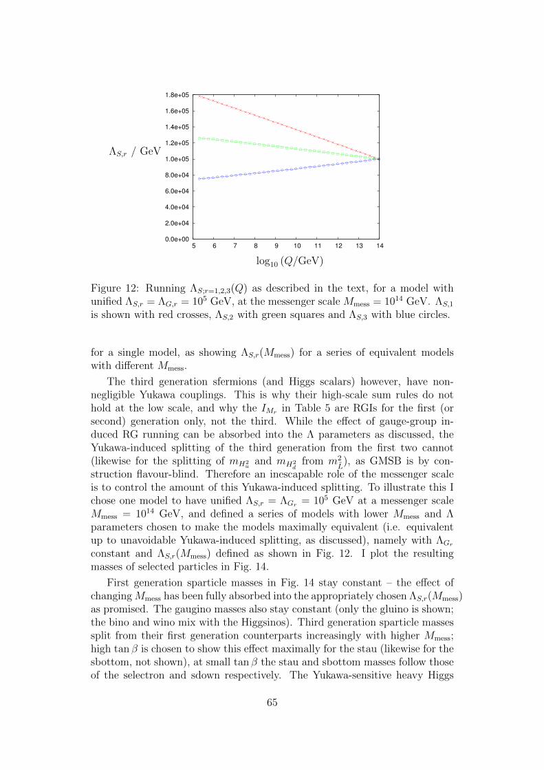
0.0e+00

2.0e+04

4.0e+04

6.0e+04

8.0e+04

1.0e+05

1.2e+05

1.4e+05

1.6e+05

1.8e+05

5 6 7 8 9 10 11 12 13 14

ΛS,r / GeV

log10 (Q/GeV)

Figure 12: Running ΛS;r=1,2,3(Q) as described in the text, for a model withunified ΛS,r = ΛG,r = 105 GeV, at the messenger scale Mmess = 1014 GeV. ΛS,1

is shown with red crosses, ΛS,2 with green squares and ΛS,3 with blue circles.

for a single model, as showing ΛS,r(Mmess) for a series of equivalent modelswith different Mmess.

The third generation sfermions (and Higgs scalars) however, have non-negligible Yukawa couplings. This is why their high-scale sum rules do nothold at the low scale, and why the IMr in Table 5 are RGIs for the first (orsecond) generation only, not the third. While the effect of gauge-group in-duced RG running can be absorbed into the Λ parameters as discussed, theYukawa-induced splitting of the third generation from the first two cannot(likewise for the splitting of mH2

uand mH2

dfrom m2

L), as GMSB is by con-

struction flavour-blind. Therefore an inescapable role of the messenger scaleis to control the amount of this Yukawa-induced splitting. To illustrate this Ichose one model to have unified ΛS,r = ΛGr = 105 GeV at a messenger scaleMmess = 1014 GeV, and defined a series of models with lower Mmess and Λparameters chosen to make the models maximally equivalent (i.e. equivalentup to unavoidable Yukawa-induced splitting, as discussed), namely with ΛGr

constant and ΛS,r(Mmess) defined as shown in Fig. 12. I plot the resultingmasses of selected particles in Fig. 14.

First generation sparticle masses in Fig. 14 stay constant – the effect ofchangingMmess has been fully absorbed into the appropriately chosen ΛS,r(Mmess)as promised. The gaugino masses also stay constant (only the gluino is shown;the bino and wino mix with the Higgsinos). Third generation sparticle massessplit from their first generation counterparts increasingly with higher Mmess;high tan β is chosen to show this effect maximally for the stau (likewise for thesbottom, not shown), at small tan β the stau and sbottom masses follow thoseof the selectron and sdown respectively. The Yukawa-sensitive heavy Higgs

65

QMmess

ΛS,r(Mmess)ΛS,r

ΛS,r

QM ′mess

Λ′S,r(M′mess)ΛS,r

Figure 13: The running ΛS;r=1,2,3(Q) for two models with different messengerscales and different values of ΛS,r at the messenger scale, but with matchingΛS,r(Q) below the smaller messenger scale M ′

mess.

mass also varies.

The goodness of the sum rules for the first two generations, and hencethe continued parameterisation of the five mass-squareds in terms of runningΛS,r(Q), allows for a potential signature for unified ΛS,r(Mmess) = ΛS(Mmess)models. If first/second generation superpartners were discovered, and theirmasses measured and found to satisfy the sum rules, then the low-scale ΛS,r

could be calculated. Discovery and measurement of the masses of gauginos(complicated by the need to determine the mixing angles with Higgsinos) wouldthen determine the running ΛS,r(Q) up to high scales. If these three quantitieswere observed to unify at a single scale, this would be suggestive of a unifiedΛS GGM model with a messenger mass at the observed unification scale. Notethat unification of running ΛS,r(Q) is a separate issue from gauge-couplingunification: one may happen without the other, and the unification scales areindependent. Explicitly, from the definition of the IMr in Table 5 and thedefinition of running ΛS,r(Q) in Eq. (5.3), the values of ΛS,r at a low scale Qlow

are determined by measurement as

Λ2S,r(Qlow) =

16π2

κrα2r(Qlow)

∑f

D(f , r)m2f ,1

(Qlow) (5.4)

These can be extrapolated up to any higher scale Q by replacing Qlow with Qthroughout, of course; however knowing the one-loop running of the sfermionmass-squareds and gauge couplings this gives explicitly

Λ2S,r(Q) =

16π2

κrα2r(Qlow)

∑f

D(f , r)m2f ,1

(Qlow) +M2r (Qlow)

(1− α2

r(Qlow)

α2r(Q)

)(5.5)

66

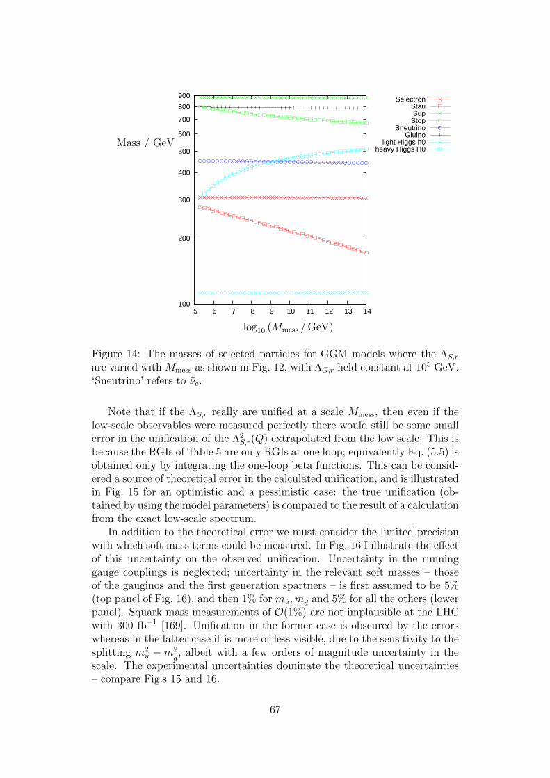
100

200

300

400

500

600

700

800

900

5 6 7 8 9 10 11 12 13 14

SelectronStauSupStop

SneutrinoGluino

light Higgs h0heavy Higgs H0

Mass / GeV

log10 (Mmess /GeV)

Figure 14: The masses of selected particles for GGM models where the ΛS,r

are varied with Mmess as shown in Fig. 12, with ΛG,r held constant at 105 GeV.‘Sneutrino’ refers to νe.

Note that if the ΛS,r really are unified at a scale Mmess, then even if thelow-scale observables were measured perfectly there would still be some smallerror in the unification of the Λ2

S,r(Q) extrapolated from the low scale. This isbecause the RGIs of Table 5 are only RGIs at one loop; equivalently Eq. (5.5) isobtained only by integrating the one-loop beta functions. This can be consid-ered a source of theoretical error in the calculated unification, and is illustratedin Fig. 15 for an optimistic and a pessimistic case: the true unification (ob-tained by using the model parameters) is compared to the result of a calculationfrom the exact low-scale spectrum.

In addition to the theoretical error we must consider the limited precisionwith which soft mass terms could be measured. In Fig. 16 I illustrate the effectof this uncertainty on the observed unification. Uncertainty in the runninggauge couplings is neglected; uncertainty in the relevant soft masses – thoseof the gauginos and the first generation spartners – is first assumed to be 5%(top panel of Fig. 16), and then 1% for mu,md and 5% for all the others (lowerpanel). Squark mass measurements of O(1%) are not implausible at the LHCwith 300 fb−1 [169]. Unification in the former case is obscured by the errorswhereas in the latter case it is more or less visible, due to the sensitivity to thesplitting m2

u − m2d, albeit with a few orders of magnitude uncertainty in the

scale. The experimental uncertainties dominate the theoretical uncertainties– compare Fig.s 15 and 16.

67

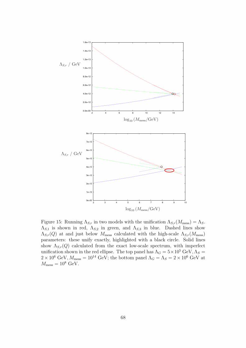
0.0e+00

2.0e+12

4.0e+12

6.0e+12

8.0e+12

1.0e+13

1.2e+13

1.4e+13

1.6e+13

2 4 6 8 10 12 14

ΛS,r / GeV

log10(Mmess/GeV)

0e+00

1e+12

2e+12

3e+12

4e+12

5e+12

6e+12

7e+12

8e+12

2 3 4 5 6 7 8 9 10

ΛS,r / GeV

log10(Mmess/GeV)

Figure 15: Running ΛS,r in two models with the unification ΛS,r(Mmess) = ΛS.ΛS,1 is shown in red, ΛS,2 in green, and ΛS,3 in blue. Dashed lines showΛS,r(Q) at and just below Mmess calculated with the high-scale ΛS,r(Mmess)parameters: these unify exactly, highlighted with a black circle. Solid linesshow ΛS,r(Q) calculated from the exact low-scale spectrum, with imperfectunification shown in the red ellipse. The top panel has ΛG = 5×105 GeV,ΛS =2× 106 GeV,Mmess = 1014 GeV; the bottom panel ΛG = ΛS = 2× 106 GeV atMmess = 108 GeV.

68

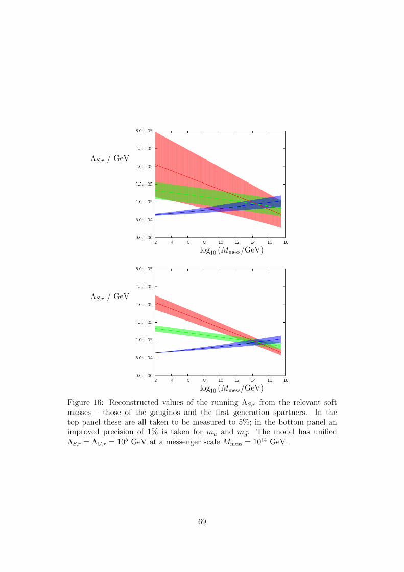
ΛS,r / GeV

log10 (Mmess/GeV)

ΛS,r / GeV

log10 (Mmess/GeV)

Figure 16: Reconstructed values of the running ΛS,r from the relevant softmasses – those of the gauginos and the first generation spartners. In thetop panel these are all taken to be measured to 5%; in the bottom panel animproved precision of 1% is taken for mu and md. The model has unifiedΛS,r = ΛG,r = 105 GeV at a messenger scale Mmess = 1014 GeV.

69

Part IV

Susy Searches At The LHC

6 Introduction

6.1 How To (Not) See Susy

Proton collisions at the LHC may produce Susy particles if they exist withmasses around the weak/TeV scale. The final state(s) they decay into willthen be enriched compared to the Standard Model22, or said another way,signal plus background is greater than background alone. In order to havethis effect be as visible as possible, we typically try to find the point in phasespace (see the glossary) with the largest ratio of signal plus background tobackground, and focus on a region of phase space around that point which issmall enough to retain this large ratio, but large enough for it to correspond toa statistically significant number of events N when multiplied by our envisagedintegrated luminosity L: N = L × σ, where sigma has been integrated overthe chosen phase space.

Once one has a rough idea of the region of phase space to focus on, furtherdiscrimination of signal plus background from background alone may be pos-sible if there is an observable (a quantity typically calculated from the finalstate four-momenta) which is distributed very differently in the two cases. Theclassic example is the invariant mass of the sum of the four-momenta of all theparticles into which a new particle decays: by definition this is a δ-functionfor the signal, smeared out both by the finite width of the particle and bydetector resolution, and some more broadly spread continuous distribution forthe background. It is thus highly desirable to calculate this observable notonly to know the mass of any particles that might be discovered this way, butbecause it is essentially the ideal way to discover their existence in the firstplace, by concentrating all of the signal to a highly visible bump on a smoothbackground.

Mass reconstruction is generally not possible however when the particlewe’re searching for decays to neutral particles that are stable on a collidertimescale, as such particles are not detected. As mentioned in Section 1.1, forR parity conserving Susy the LSP is stable, and therefore it must be neutral forconsistent cosmology. Unless decays to the LSP are strongly suppressed, i.e thenext-to-LSP (NLSP) or NNLSP etc. is quasi-stable, any sparticles producedat a collider will decay to an invisible LSP inside the detector. FurthermoreR parity ensures sparticles can only be produced in pairs, and so all events

22This is is not a given in quantum field theory of course – a cross-section is the square-modulus of a sum of amplitudes A, and these may interfere destructively. It is almost alwaysthe case however that the final states resulting from the decays of BSM particles are enhancedcompared to the Standard Model alone, i.e. that |Asignal +Abackground|2 > |Abackground|2.

70

will result in pairs of LSPs. Mass peaks are therefore typically a pipe dreamfor R parity conserving Susy, though see Section 8 in which the dream comestrue in the specific case of boosted decays.

Without mass peaks we are often forced into cut and count style approaches:we identify the aforementioned roughly selected region of phase space whichis promising, ignore/cut the rest of phase space, and simply count events. Ifthe number of events observed closely matches the number predicted by thebackground alone, then any new physics which predicts considerably moreevents than this can be excluded. The problem with such analyses is that weneed precise knowledge of the background normalisation – the integral of thebackground differential cross-section over the selected phase space. To see thisnote that a even a modest error in the background differential cross-section,when integrated over a large phase space, could result in an uncertainty thatswallows the whole signal (which may live only in a certain part of the phasespace though we don’t know where). This is to be contrasted with the presenceor absence of a bump on top of a smooth function (the background), which isnot sensitive to an overall scaling of the latter.

Cut and count analyses do however lead to exclusion limits which arestraightforward to re-interpret in other models: they set an upper limit, ata certain confidence level which is usually chosen to be 95%, on the cross-section that any new physics can contribute to the final states and region ofphase space that pass the cuts. Said more precisely the upper limit is on thequantity σprod × A × ε, where σprod is the production cross-section for newphysics, A is the acceptance, and ε is the efficiency i.e. the ratio of the num-ber of events that should pass the cuts to the number that actually do, due toimperfections of the detector. Writing this product as σsignal, new physics withσlimit/σsignal less than (greater than) one is excluded (allowed). The bound-ary/boundaries between such regions are often illustrated with Brazil-bandplots, which I explain in a manner suitable for novices in Appendix C.

6.2 Complications At NLO

To interpret a model-independent cross-section upper limit in a specific model,we need to know the model’s acceptance, and so we need the distributions inphase space resulting from production and decay of our new hypothesisedparticles. This problem is almost always tackled by using Monte Carlo eventgenerators to simulate large numbers of events (particle collisions in the mannerof the chosen collider – here the LHC). In a nut-shell, an event generatorsimulates a single event by considering what could happen each time particlesinteract (a typical event involves a huge number of interactions), and choosingone of the possibilities randomly but weighted by the physical probabilitywhich has been calculated using QFT. The user may force all of the eventsto go down a certain pathway on the branching tree of possibilities, which issensible if only a subset of all possible outcomes are to be studied; a scalingof final cross-sections is then appropriate to account for this. For example, in

71

studies of decays of the Higgs to a given final state, the user would normallyforce the event generator to only decay the Higgs to that final state, andmultiply any final cross-sections obtained by the branching ratio for such adecay. A second example, more relevant here, is that to study decays of Susyparticles, one should force the event generator to simulate only events whereSusy particles are produced, rather than events where the colliding particlesinteract in any way possible!

Most Monte Carlo event generators work with LO matrix elements (seethe glossary) for the production of Susy particles. NLO corrections can besubstantial however, with K-factors of 2-3 common for total cross-sections forproduction of coloured sparticles. A common approach is then to calculateσsignal = σprod × A (neglecting non-unit efficiencies ε 6= 1 for the moment) atLO using event generation, and then to multiply by the global K-factor definedfor the total cross-section: K = σNLO/σLO. There are two ways in which thiscan fail as an approximation for σsignal at truly NLO.

• High phase space dependence of K. It is clear that to convert σsignal fromLO to NLO we should multiply it by the K-factor associated with theregion of phase space we are concerned with, not the K-factor associatedwith an integral over all phase space. The latter is only acceptable if thetwo K-factors are similar. (As an example of when this is not the casesee the O(10−100) K-factor in the high-pT tail of light slepton Drell-Yanproduction shown in [170].)

• High dependence of both K and acceptance on particle-species. σsignal

may receive contributions from the production and subsequent decay ofdifferent new particles; let me say via different channels for brevity. Ifdifferent channels have different K-factors and different acceptances, thenmultiplying the cross-section for the full signal (including all channels)by the total K-factor is not correct23, as the following toy example shows.Say our signal receives contributions from electroweak production (‘EW’)and coloured production (‘C’) and we use a search strategy geared moretowards one than the other, say vetoing leptons, giving a higher accep-tance for the latter than the former: AC > AEW . The strength of thestrong interaction means that generically KC > KEW ; so we have chan-nels with different acceptances and K-factors. For concreteness let ustake the cross-sections to be

σC,LO = σEW,LO, (6.1)

KC = 3, KEW = 1 (6.2)

∴ Ktot = σtot,NLO / σtot, LO = 2, (6.3)

where we assume interference diagrams to be negligible so thatσtot = σC + σEW . Take the (a priori unknown) acceptances to beAC = 1,

23Thanks to Peter Richardson for realising this in the context of our work, and to DavidGrellscheid for patiently explaining it to me.

72

AEW = 0. Monte Carlo simulation (at LO) of both channels simultane-ously will generate equal numbers of events for each (as σC,LO = σEW,LO),and since AC = 1, AEW = 0 the total acceptance is determined to beAtot = 0.5. The LO signal cross-section is then σint, LO = σtot, LO × Atot;multiplying by the total K-factor one erroneously concludes

σint,NLO!

= σtot, LO × Atot ×Ktot in general, (6.4)

= 2σC,LO in this example. (6.5)

This should be compared with what is clearly the correct answer, ob-tained by simulating the two channels separately in order to determinetheir individual acceptances, then weighting each by its individual K-factor:

σint,NLO =∑

i=C,EW

σi, LO × Ai ×Ki in general, (6.6)

= 3σC,LO in this example, (6.7)

where i denotes the channel. To see more clearly the difference betweenthe two approaches, and when they coincide, I re-write Eq. (6.4) explic-itly denoting was is meant by the total acceptance and K-factor in termsof the channel-by-channel definition of these quantities:

σint,NLO!

= σtot, LO × Atot ×Ktot

=

(∑i

σi, LO

)×(∑

i σi, LOAi∑i σi, LO

)×(∑

i σi, LOKi∑i σi, LO

)=

(∑

i σi, LOAi) (∑

i σi, LOKi)∑i σi, LO

(6.8)

The incorrect combined channel approach, Eq. (6.8), coincides with thecorrect channel-by-channel approach, Eq. (6.6), if there is a commonacceptance across all channels Ai = A or if there is a common K-factoracross all channels Ki = K.

In the event generation of Section 7 I will not address the issue of phase spacedependent K-factors. I will however take into account the issue of non-universalK-factors and acceptances across different channels.

6.3 The Importance Of The LSP

Spontaneous breaking of a global supersymmetry results in a massless fermioncalled the Goldstino; this is just Goldstone’s Theorem applied to a brokenfermionic generator. In the context of gravity Susy must be promoted to alocal symmetry (supergravity) with the the spin-3

2superpartner of the graviton

– the gravitino – acting as the associated gauge field. Upon spontaneous

73

breaking of the local supersymmetry the massless gravitino eats the would-be Goldstino to obtain mass and longitudinal components: this is called theSuper-Higgs mechanism, being a close parallel of the Higgs- or more justlythe Brout-Englert-Higgs mechanism [171, 172, 173] in which a spin-one gaugeboson obtains mass and a longitudinal component by eating a scalar. Thetransverse components of the gravitino interact only gravitationally, and so itsinteractions are dominantly just those of its Goldstino component (and thedistinction between gravitino and Goldstino is irrelevant, with both usuallydenoted G). With Susy breaking coming from a single F -term VEV, 〈F 〉, theresulting gravitino mass can be estimated from dimensional analysis [174, 175]as

m3/2 ∼ 〈F 〉/MP , (6.9)

as it must vanish in the limit of decoupled gravity MP → ∞ or restoredSusy 〈F 〉 → 0. The other superpartners however receive masses ∼〈F 〉/Mmess,suppressed only by the mass Mmess of the Susy-breaking mediator. In GMSBthis is much below MP , and so the gravitino is always the LSP.

The decay of a sparticle to its Standard Model partner and the gravitinois suppressed, having decay width [6]

Γ(X → XG) =m5X

16π〈F 〉2(1−m2

X/m2X

)4 (6.10)

For GMSB with mX ∼ 〈F 〉/Mmess, the suppressing factor is m4X/〈F 〉2 ∼

〈F 〉2/M4mess, which we typically take much less than one as discussed in Sec-

tion 4.2. Therefore the dominant decay cascades (see the glossary) for R par-ity conserving GMSB will be those where each pair-produced particle decaysthrough a series of steps with gauge or Yukawa vertices until the NLSP isproduced, and only then does the decay to the gravitino occur, as no otherchannel competes. GMSB collider phenomenology then depends most impor-tantly on the NLSP species (i.e. the identity of X, and thus X, in X → XG)and whether or not this decay is sufficiently suppressed as to occur outside thedetector. In [176] the associated decay length for ΛS,ΛG models is given as

LNLSP ∼1

k2G

(100 GeV

mNLSP

)5( √ΛGM

105 GeV

)4

10−4 m, (6.11)

where kG (the reciprocal of the parameter known as Cgrav) quantifies the cou-pling of messengers to the Susy-breaking sector, which may be O(1) or muchsmaller. For ΛG ∼ 105 GeV, messenger scales Mmess & 107 GeV lead toLdecay & 10 m and a decay outside of the detector. When kG 1 even smallervalues of the Mmess may suffice. Detector-stable NLSPs are therefore a veryrealistic possibility. The NLSP species in these models can be crudely char-acterised as a bino-like χ0

1 for ΛG . ΛS and a charged slepton for ΛG & ΛS

(specifically a stau for large tan β and slepton-smuon-stau co-NLSP for smalltan β). Detector-stable charged particles have dedicated searches; a detector-stable χ0

1 however will manifest itself via missing energy.

74

7 A Historical Detour: Comparing Early LHC

Direct Searches To LEP Higgs Bounds

This section is based on my work [114] done in collaboration with David Grellscheid,Jorg Jackel, Valya Khoze and Peter Richardson; the text has been mostly re-written.

7.1 Introduction And Main Results

The final state in which we initially harboured the most hope for seeing Susyat the LHC was jets, /ET , and no leptons.

• Jets. The particles with the largest production cross-sections for a givenmass are coloured particles, since QCD is the strongest interaction atthe weak/TeV scale and at the LHC we collide coloured objects. De-cays of coloured particles must produce other coloured particles (as thecolour quantum number is conserved), which will ultimately hadroniseto produce jets.

• /ET . Susy is most often considered in the R parity conserving scenario, sothat the LSP is stable and constitutes a dark matter candidate. Providedthe full decay cascade is prompt (takes place inside the detector), theescape of the two LSPs gives rise to /ET . To give large /ET , the LSPsmust carry appreciable kinetic energy (and not be back-to-back in thetransverse plane), which requires the initially produced particles to beappreciably more massive than the sum of the masses of all final stateparticles.

• No leptons. Backgrounds are either reducible or irreducible (see the glos-sary). The irreducible background for /ET consists exclusively ofW and Zbosons decaying to neutrinos. A neutrino from a decaying W is accompa-nied by a lepton, unless it is ντ and the associated τ decays hadronically.Thus for new physics decays that produce /ET without leptons, such asthe squark and gluino decays q → qχ0

1 and g → qqχ01, a lepton veto will

generally improve the ratio of signal to (reducible) background.

Though discovery and exclusion do not have trivially connected statistics(e.g. the confidence level for discovery plus the confidence level for exclusiondoes not equal one!), a search strategy with strong potential for discovery willalso be able to set strong exclusion limits (unless the hypothetical particleactually exists of course) and vice versa, since both of these come if and onlyif the strategy has sensitivity to the hunted particle’s signal. Therefore whendata in the much anticipated jets, /ET and no-lepton (henceforth jets+ /ET )channels began coming in in earnest but without excesses over the background,strong exclusion bounds were set (and are continuing to be set of course).

75

In [114] I compared the strongest such bounds from 2011 – those obtainedin 1.04 fb−1 of data taken in 7 TeV collisions (and focussing on the ATLASCollaboration’s results [177]) – to the LEP limit on a Higgs with StandardModel-like couplings, mh > 114.4 GeV [178]. This was done for models ofGMSB parameterised by ΛS,ΛG,Mmess and tan β (see Part III) and for theConstrained Minimal Supersymmetric Standard Model (CMSSM, see e.g. [6]).The sign of the µ parameter was taken to be +1 throughout. The results areshown in Fig. 17, with the exclusion contours projected on the squark-gluinomass plane24. Explanations and interpretations of these bounds follow.

For the GMSB case, as mentioned, the NLSP in these models is generallyeither a bino-like neutralino or a charged slepton, and may be quasi-stable ordecay promptly. Charged sleptons, when decaying promptly, produce a grav-itino (seen as /ET ) and a charged lepton; when stable a charged non-hadronictrack is seen to leave the detector. Promptly decaying bino-like neutralinosproduce a gravitino usually with a photon (G + Z becomes competitive forheavy neutralinos). I focussed on a detector-stable neutralino as the NLSP,which gives large /ET that is not shared with a hard and distinctive lepton orphoton, and so is most appropriate for constraining by a jets+/ET search.

7.2 Derivation Of The Exclusion Contours

My route to obtaining the jets+ /ET constraints followed [181] closely25:

• Low-scale Susy spectra were calculated from high-scale model input usingSOFTSUSY 3.1.6.

• Signal events were generated with Herwig++ 2.5.1, separated into sam-ples of (a) pair-produced squarks and/or gluinos, (b) pair-produced slep-tons, neutralinos and/or charginos, and (c) one squark or gluino producedwith one slepton, neutralino or chargino. (c) typically has negligiblecross-section in these scenarios. (b) may have comparable cross-sectionto (a) but is largely eliminated by a lepton veto; given this differencein acceptance (and the obvious difference in K-factors), the argument ofSection 6 shows the importance in separating these production channels.

• High-level objects (see the glossary) were defined from the final stateparticles using the RIVET 1.5.2 analysis framework and FastJet [183].The cuts for each search channel were also imposed with RIVET; thesecuts are detailed in Appendix D. The fraction of events passing the cutsfor each channel is the acceptance.

24Thanks to Jorg Jackel for providing the gradient of the RG-inaccessible region.25I am grateful to David Grellscheid and Peter Richardson for providing the code necessary

for Prospino cross-section calculation and Susy event generation with Herwig++ and RIVET

on The Grid [182].

76

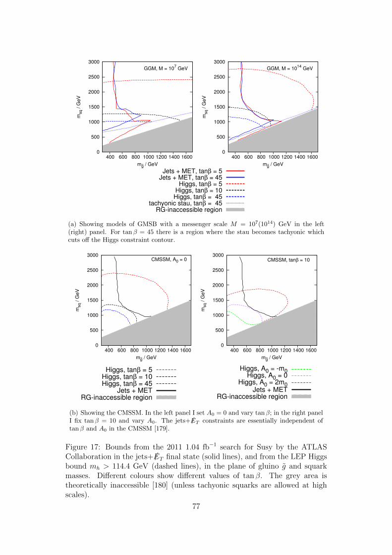
0

500

1000

1500

2000

2500

3000

400 600 800 1000 1200 1400 1600

msq / G

eV

mg~ / GeV

GGM, M = 107 GeV

0

500

1000

1500

2000

2500

3000

400 600 800 1000 1200 1400 1600

msq / G

eV

mg~ / GeV

GGM, M = 1014

GeV

0 500

1000 1500 2000 2500 3000

400 600 800 1000 1200 1400 1600

msq / G

eV

mg~ / GeV

Jets + MET, tanβ = 5Jets + MET, tanβ = 45

Higgs, tanβ = 5Higgs, tanβ = 10

Higgs, tanβ = 45tachyonic stau, tanβ = 45

RG-inaccessible region

(a) Showing models of GMSB with a messenger scale M = 107(1014) GeV in the left(right) panel. For tanβ = 45 there is a region where the stau becomes tachyonic whichcuts off the Higgs constraint contour.

0

500

1000

1500

2000

2500

3000

400 600 800 1000 1200 1400 1600

msq / G

eV

mg~ / GeV

CMSSM, A0 = 0

0

500

1000

1500

2000

2500

3000

400 600 800 1000 1200 1400 1600

msq / G

eV

mg~ / GeV

CMSSM, tanβ = 10

0

500

1000

1500

2000

2500

3000

400 600 800 1000 1200 1400 1600

msq / G

eV

mg~ / GeV

Higgs, tanβ = 5Higgs, tanβ = 10Higgs, tanβ = 45

Jets + METRG-inaccessible region

0

500

1000

1500

2000

2500

3000

400 600 800 1000 1200 1400 1600

msq /

Ge

V

mg~ / GeV

Higgs, A0 = -m0Higgs, A0 = 0

Higgs, A0 = 2m0Jets + MET

RG-inaccessible region

(b) Showing the CMSSM. In the left panel I set A0 = 0 and vary tanβ; in the right panelI fix tanβ = 10 and vary A0. The jets+/ET constraints are essentially independent oftanβ and A0 in the CMSSM [179].

Figure 17: Bounds from the 2011 1.04 fb−1 search for Susy by the ATLASCollaboration in the jets+ /ET final state (solid lines), and from the LEP Higgsbound mh > 114.4 GeV (dashed lines), in the plane of gluino g and squarkmasses. Different colours show different values of tan β. The grey area istheoretically inaccessible [180] (unless tachyonic squarks are allowed at highscales).

77

• NLO production cross-sections were calculated with Prospino 2.1; anindication of theoretical uncertainty was given by varying the renormali-sation/factorisation scale by factors of 2±1. Multiplying the cross-sectionby the acceptance defined our σsignal, which was compared to the exper-imentally determined σlimit.

• The previous steps were done for the same plane in Susy model space asused by the experimental collaboration to present its own results. Witha close matching of the original and reproduced exclusion contours, thereproduced search channels can be considered validated. In the presentcase this agreement is shown in Fig. 18, giving confidence in my repro-duction of the jets+/ET search channels (which we then made publiclyavailable as part of RIVET package: analysis ATLAS 2011 S9212183).

• With the previous step validating those that came before, the same pro-cedure can then be followed for other Susy models which were not con-sidered by the experimental collaboration.

As discussed in Ref. [177] a localised detector failure caused a loss of jetenergy and “a loss of signal acceptance which is smaller than 15% for the mod-els considered”. This was taken into account here by including an efficiencyfactor ε = 0.85 in σsignal ≡ σprod ×A× ε, for four of the five different channels– all except the High Mass channel. The latter places the strongest demandson jet multiplicity (see the glossary) and pT ; as can be seen from Fig. 18 thelocation of the resulting exclusion contour has large uncertainties26. Includingan efficiency factor in this way gave a minor improvement to my agreementwith the ATLAS Collaboration’s bounds in the same plane.

To check exclusion by Higgs-based searches I used FeynHiggs 2.8.5 tocalculate Higgs-sector masses, couplings and cross-sections, and passed theseto HiggsBounds 3.5.0beta to compare with a comprehensive set of exper-imental limits from LEP, the Tevatron and the LHC. HiggsBounds returnsσsignal/σlimit for the search channel with the highest statistical sensitivity: aratio greater than 1 indicates 95% confidence-level exclusion by at least onesearch. Note that this does not take into account a kind of look elsewhere effectthat arises when one checks many different independent searches for the pres-ence of a single one indicating exclusion. A statistically thorough approachwould calculate the full combined likelihood for all of the observed experimen-tal results given the hypothesis of the model in question, and see whether thiscorresponds to a probability less than the critical value (nominally 0.05); thisis beyond the scope of HiggsBounds.

26This is because these demanding cuts mean the acceptance is a steeply rising functionof sparticle mass in the part of the plane where σsignal ∼ σlimit; the product of acceptanceand production cross-section (with the latter always falling steeply with mass) is then fairlyflat around σprod × A ∼ σlimit, and a systematic shift in this product (such as an efficiencyfactor or σprod scale uncertainties) can move this flat region from having σprod ×A . σlimit

to σprod ×A & σlimit, causing a large shift in the exclusion contour.

78

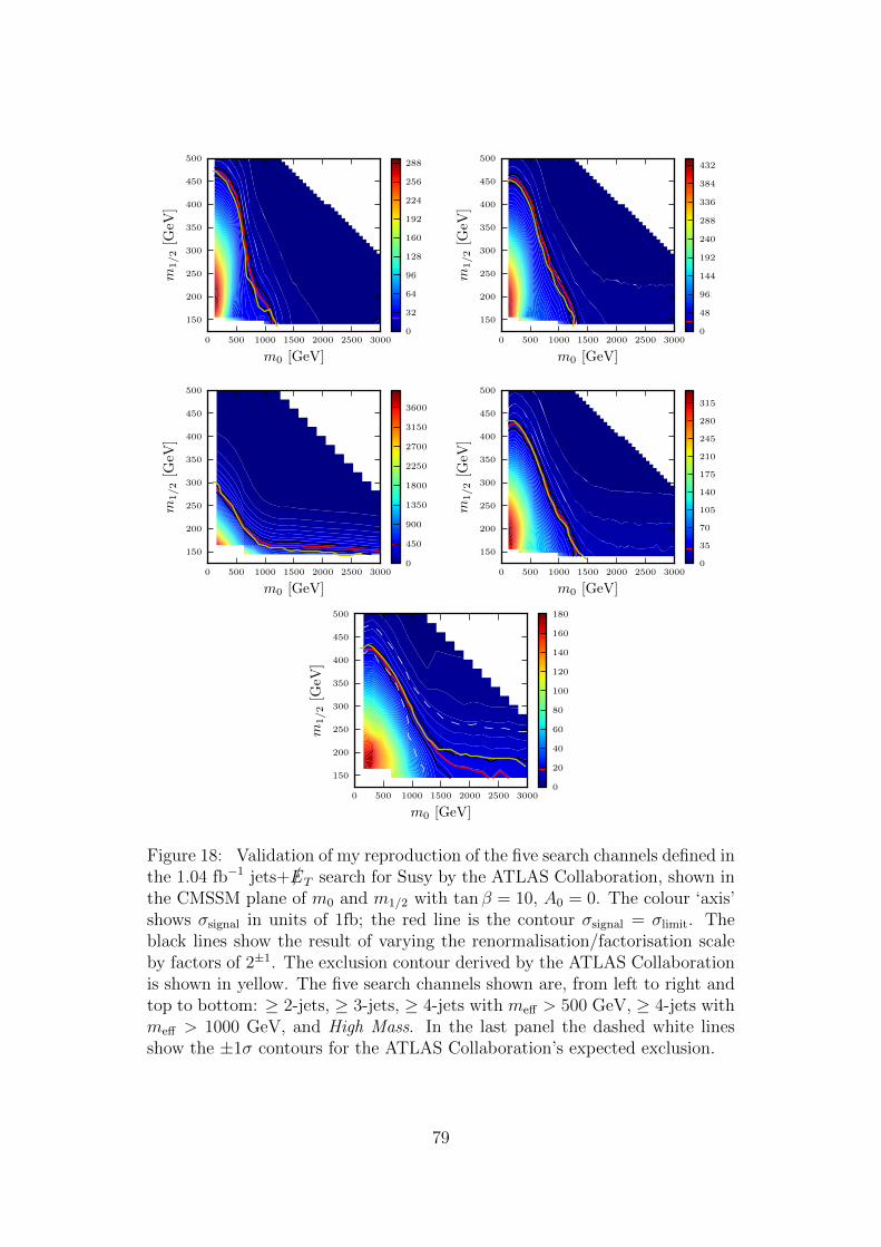
0 500 1000 1500 2000 2500 3000

m0 [GeV]

150

200

250

300

350

400

450

500m

1/2

[GeV

]

0

32

64

96

128

160

192

224

256

288

0 500 1000 1500 2000 2500 3000

m0 [GeV]

150

200

250

300

350

400

450

500

m1/2

[GeV

]

0

48

96

144

192

240

288

336

384

432

0 500 1000 1500 2000 2500 3000

m0 [GeV]

150

200

250

300

350

400

450

500

m1/2

[GeV

]

0

450

900

1350

1800

2250

2700

3150

3600

0 500 1000 1500 2000 2500 3000

m0 [GeV]

150

200

250

300

350

400

450

500

m1/2

[GeV

]

0

35

70

105

140

175

210

245

280

315

0 500 1000 1500 2000 2500 3000

m0 [GeV]

150

200

250

300

350

400

450

500

m1/2

[GeV

]

0

20

40

60

80

100

120

140

160

180

Figure 18: Validation of my reproduction of the five search channels defined inthe 1.04 fb−1 jets+ /ET search for Susy by the ATLAS Collaboration, shown inthe CMSSM plane of m0 and m1/2 with tan β = 10, A0 = 0. The colour ‘axis’shows σsignal in units of 1fb; the red line is the contour σsignal = σlimit. Theblack lines show the result of varying the renormalisation/factorisation scaleby factors of 2±1. The exclusion contour derived by the ATLAS Collaborationis shown in yellow. The five search channels shown are, from left to right andtop to bottom: ≥ 2-jets, ≥ 3-jets, ≥ 4-jets with meff > 500 GeV, ≥ 4-jets withmeff > 1000 GeV, and High Mass. In the last panel the dashed white linesshow the ±1σ contours for the ATLAS Collaboration’s expected exclusion.

79

Higgs constraints were checked with HiggsBounds because, in general, lim-its are fundamentally set in terms of cross-sections. Their interpretation asmass limits is always a model-dependent process, requiring assumptions aboutcouplings and branching ratios. The LEP bound mh > 114.4 GeV applies toa Standard Model-like Higgs, and carries across to a Susy Higgs only in thedecoupling limit and when h has no BSM decay channels open. For the mod-els investigated here this was the case: the HiggsBounds result simplified to acomparison of mh with 114.4 GeV. However away from the decoupling limit,and/or with h → BSM possible, and/or with the LEP constraint being su-perseded by LHC Higgs results (which are incorporated in updated versions ofHiggsBounds), this check will not in general be so trivial. It is facilitated by mycode available at [131] which links SOFTSUSY to FeynHiggs and HiggsBounds

with automated plotting of the results.

7.3 Interpretation Of The Exclusion Contours

The most basic point to note is that large masses for squarks and gluinosmake it easier to satisfy both jets+/ET and mh constraints. Coloured spar-ticles being heavy helps to avoid jets+/ET constraints because this decreasessignal production cross-section. Heavy squarks boost mh because of the stop’spositive contribution to δmh, and the fact that both GMSB and the CMSSMare flavour-blind (at the high-scale at least – this is slightly detuned by theStandard Model Yukawa couplings during RG running), tying the stop massto the general squark mass. Heavy gluinos may help boost mh because theycontribute to the negative running of At from high to low scale, thus increas-ing the latter’s absolute value at the low scale (provided it is negative), andfor constant stop mass, mh increases27 with |At|. This effect is clearly en-hanced for more RG running, and indeed we see that for heavy gluinos theLEP bound is less constraining for high messenger scale than low messengerscale: in Fig. 17(a) the dashed lines are flatter in the left panel whereas theyfall off for large mg in the right panel.

In addition to the squark and gluino masses, which are dominantly set bythe mass parameters m0,m1/2 in the CMSSM and their counterparts ΛS,ΛG

in these GMSB models, there are two further free parameters in each case:tan β,A0 in the CMSSM and tan β,Mmess for GMSB. In the CMSSM casethese extra parameters were shown in [179] to have essentially no effect on thejets+/ET constraints. As can be seen in Fig. 19, the parameters tan β,Mmess

27Unless of course |At| is increased beyond√

6MS . In GGM however we start from At = 0at a high scale, and boosting its low scale value with a large gluino mass and/or many decades(see the glossary) of running will simultaneously boost the low scale stop mass which alsoruns strongly with mg, generically forcing At/MS <

√6 [184]. This conclusion is escaped

if we allow the stops to be tachyonic at the high scale, which unties the low-scale MS fromAt [185]. This implies the existence of other vacua beside our own in which charge andcolour are broken, however cosmological constraints may allow such a situation [186].

80

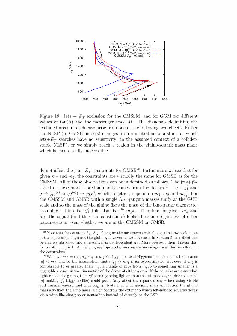
800

1000

1200

1400

1600

1800

2000

400 500 600 700 800 900 1000 1100 1200

msq /

Ge

V

mg~ / GeV

GGM, M = 107 GeV, tanβ = 5

GGM, M = 107 GeV, tanβ = 45

GGM, M = 1014

GeV, tanβ = 5GGM, M = 10

14 GeV, tanβ = 45

CMSSM, A0 = 0, tanβ = 10

Figure 19: Jets + /ET exclusion for the CMSSM, and for GGM for differentvalues of tan(β) and the messenger scale M . The diagonals delimiting theexcluded areas in each case arise from one of the following two effects. Eitherthe NLSP (in GMSB models) changes from a neutralino to a stau, for whichjets+/ET searches have no sensitivity (in the assumed context of a collider-stable NLSP), or we simply reach a region in the gluino-squark mass planewhich is theoretically inaccessible.

do not affect the jets+/ET constraints for GMSB28; furthermore we see that forgiven mq and mg, the constraints are virtually the same for GMSB as for theCMSSM. All of these observations can be understood as follows. The jets+ /ET

signal in these models predominantly comes from the decays q → q + χ01 and

g → (qq(∗) or q ¯q(∗))→ qqχ01, which, together, depend on mq, mg and mχ0

1. For

the CMSSM and GMSB with a single ΛG, gaugino masses unify at the GUTscale and so the mass of the gluino fixes the mass of the bino gauge eigenstate;assuming a bino-like χ0

1 this also fixes29 mχ01. Therefore for given mq and

mg, the signal (and thus the constraints) looks the same regardless of otherparameters or even whether we are in the CMSSM or GMSB.

28Note that for constant ΛS ,ΛG, changing the messenger scale changes the low-scale massof the squarks (though not the gluino), however as we have seen in Section 5 this effect canbe entirely absorbed into a messenger-scale dependent ΛS . More precisely then, I mean thatfor constant mq with ΛS varying appropriately, varying the messenger scale has no effect onthe constraints.

29We have mB = (α1/α3)mg ≈ mg/6; if χ01 is instead Higgsino-like, this must be because

|µ| < mB and so the assumption that mχ01≈ mB is an overestimate. However, if mq is

comparable to or greater than mg, a change of mχ01

from mg/6 to something smaller is anegligible change in the kinematics of the decay of either q or g. If the squarks are somewhatlighter than the gluino, then χ0

1 actually being lighter than the estimate mg/6 (due to a small|µ| making χ0

1 Higgsino-like) could potentially affect the squark decay – increasing visibleand missing energy, and thus σsignal. Note that with gaugino mass unification the gluinomass also fixes the wino mass, which controls the extent to which left-handed squarks decayvia a wino-like chargino or neutralino instead of directly to the LSP.

81

Having said that tan β does not affect the jets+ /ET constraints, it doeshowever control the boundary between the qualitatively different regions wherethe neutralino is the NLSP and where a charged slepton(s) is the NLSP. This isbecause large tan β enhances the tau Yukawa and the negative contribution itgives to running stau mass. This particular search does not have sensitivity toa quasi-stable charged slepton NLSP and does not constrain the correspondingparameter space, hence the tan β-dependence of the straight diagonal edge tothe GMSB jets+/ET exclusion contours.

The aforementioned ‘extra’ parameters – tan β,A0 in the CMSSM andtan β,Mmess for GMSB – do however affect the Higgs constraints.

• Larger Mmess is helpful if mg is also large, as discussed.

• Large tan β increases mh at tree-level.

• A0 is driven negative by the gluino during running, and so given thebenefit of sizable |At|/MS at low scale to boost mh, the CMSSM casesA0 = −m0, A0 = 0 and A0 = 2m0 have increasing difficulty meeting theLEP bound.

Each of these effects can be seen in Fig. 17.Fig. 20 shows the GMSB exclusion contours in terms of the original ΛG

and ΛS model parameters. The projection of these to the squark-gluino massplane is Fig. 17(a).

Though I have considered GMSB models with a single ΛS common to allthree gauge groups, and likewise for ΛG, the resulting exclusion contours havesome broader applicability to six-dimensional GGM parameter space. mh ismostly controlled by the mass of the squarks (truly the stop, but the squarkmasses are flavour-blind) and At. In turn, the squark mass is controlled moreby ΛS,3 (at tree-level) and ΛG,3 (at one-loop level) than by ΛS;1,2 or ΛG;1,2,and similarly At more by ΛG,3 than by ΛG;1,2, in both cases because of thedominance of α3 over α1,2. Therefore splittings of ΛG;1,2 from ΛG,3 and of ΛS;1,2

from ΛS,3 are subdominant parameters for setting the Higgs mass comparedto ΛG and ΛS, and for small splittings the same contours will hold.

Similarly the jets+ /ET signal depends most strongly on the squark andgluino masses, and thus on ΛG and ΛS (rather than splittings between thecontributions for different gauge groups). However (a) an independent ΛG,1

may be tuned to give a bino arbitrarily close in mass to the squarks or gluino,compressing the spectrum and removing the visible energy; (b) with six fullyindependent Λ parameters the NLSP has even more possible identities, manyof which correspond to signals that are most strongly constrained by dif-ferent searches, with the jets+/ET search losing sensitivity. The qualitativechanges contained within the possibility (b) represent a strong dependence ofthe squark-gluino mass-plane contours set here on the decision to consider onlya subset of the full GGM parameter space.

82

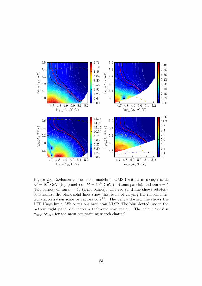
4.7 4.8 4.9 5.0 5.1 5.2

log10(ΛG/GeV)

5.0

5.1

5.2

5.3

5.4

5.5

log

10(Λ

S/G

eV)

0.00

0.64

1.28

1.92

2.56

3.20

3.84

4.48

5.12

5.76

4.7 4.8 4.9 5.0 5.1 5.2

log10(ΛG/GeV)

5.0

5.1

5.2

5.3

5.4

5.5

log

10(Λ

S/G

eV)

0.00

1.05

2.10

3.15

4.20

5.25

6.30

7.35

8.40

4.7 4.8 4.9 5.0 5.1 5.2

log10(ΛG/GeV)

4.8

5.0

5.2

5.4

5.6

log

10(Λ

S/G

eV)

0.00

1.75

3.50

5.25

7.00

8.75

10.50

12.25

14.00

15.75

4.7 4.8 4.9 5.0 5.1 5.2

log10(ΛG/GeV)

4.8

5.0

5.2

5.4

5.6

log

10(Λ

S/G

eV)

0.0

1.4

2.8

4.2

5.6

7.0

8.4

9.8

11.2

12.6

Figure 20: Exclusion contours for models of GMSB with a messenger scaleM = 107 GeV (top panels) or M = 1014 GeV (bottoms panels), and tan β = 5(left panels) or tan β = 45 (right panels). The red solid line shows jets+ /ET

constraints; the black solid lines show the result of varying the renormalisa-tion/factorisation scale by factors of 2±1. The yellow dashed line shows theLEP Higgs limit. White regions have stau NLSP. The blue dotted line in thebottom right panel delineates a tachyonic stau region. The colour ‘axis’ isσsignal/σlimit for the most constraining search channel.

83

8 Making The Most Of MET: Mass Recon-

struction From Collimated Decays

This section is based on my work [124] done in collaboration with Michael Span-nowsky; excepting the extended Introduction the text here follows it closely. Inthis section neutralinos are denoted by Ni, with χ indicating a generic invisibleparticle.

8.1 Introduction

Missing transverse energy – MET – is of great importance at hadron colliders:it is our only way of inferring the presence of neutral (collider-)stable particlesχ, be they neutrinos or BSM particles. However whenever two such particlesare produced (which will always be the case if their stability is due to a Z2

symmetry, for example) our observation only of the vectorial sum of theirtransverse momenta /pT = pa,T + pb,T thwarts reconstruction of masses in the

decay cascade30 ending with 2χ. Popular methods for searching for heavyparticles with partially invisible decays are transverse mass observables [187],MT2 [188], razor analyses [189] and kinematic edges [190]. I will introduce thefirst two of these.

Consider events with a single leptonically decaying W , Fig. 21(a), togetherwith any number of jets and photons (but not leptons: the sole lepton and /pTcan then unambiguously identified with the lepton l and neutrino ν from theW ). We have

m2W = (El + Eν)

2 − (pl + pν)2

= m2l +m2

ν + 2(ET,lET,ν cosh(∆ylν)− pT,l · pT,ν),(8.1)

where y is rapidity and ET is transverse energy –√

(m2 + p2T ). At hadron

colliders we do not know the neutrino’s momentum in the z direction and hencemW is not calculable this way. A quantity we can calculate is the transversemass mT :

m2T ≡ (ET,l + ET,ν)

2 − (pT,l + pT,ν)2

= m2l +m2

ν + 2(ET,lET,ν − pT,l · pT,ν)(8.2)

As we have just one invisible particle, pT,ν = /pT ; and since that it is massless,ET,ν = |/pT |; hence the calculability of Eq. (8.2). Comparing it to Eq. (8.1) wesee that mT ≤ mW ; an inequality which is violated by the finite width effects

302χ could also be directly produced, giving a final state with, at leading order, no largetransverse energy (visible or invisible). The universal possibility of hard initial state radia-tion allows essentially model-independent limits to be set on the direct production of new χparticles from monojet and monophoton searches. Here I will focus only on production of2χ via a decay cascade.

84

W±

l±

νl

(a)

X

vis

invis

(b)

Figure 21: Cartoons of leptonic W decay (left panel) and the decay of oneparticle X to multiple visible and multiple invisible particles (right panel).

of the W and by detector resolution effects. If the inequality were typically farfrom being saturated it would not be helpful for determining mW . Howeverthe cross-section is enhanced at mT ≈ mW [191]:

dσ

dm2eνm

2eν,T

∝ ΓWmW

(m2eν −m2

W )2 + Γ2Wm

2W

1

meν

√m2eν −m2

eν,T

, (8.3)

leading to what is called a Jacobian peak in the distribution right before theend point at mW .

Now consider a single particle X decaying into multiple visible and multipleinvisible particles, Fig. 21(b). By replacing the four-momenta of the lepton andneutrino in Eq.s (8.1) and (8.2) by the four-momenta summed over the visibleand invisible particles respectively, the same arguments give a transverse masswith a Jacobian peak and end point at mX . There is one further subtlety herehowever, in that while /pT can still be identified with the summed pT of theinvisible particles, the transverse energy of the invisible system is not given by|/pT | since the invariant mass of invisible system is in general not zero. Thelatter vanishes only if all the invisible particles are massless and travelling inexactly the same direction. In the absence of further information this must beassumed to be true; neglecting the invisible mass leads to an underestimateof the invisible transverse energy, thus smearing the Jacobian peak to valuesfurther below the end point at mX .

For two partially-invisibly decaying particles, with the example of slep-tons l decaying to leptons and neutralinos N1 shown in Fig. 22, the transversemass as defined in the previous paragraph can be calculated in the same way.However the result is now constrained to be less than or equal to the massof the two-slepton system: if the sleptons are moving relative to each other,their combined mass is not an interesting quantity. What we would like isa transverse mass associated with each separate slepton – by definition thesequantities would have end points at the slepton mass (for simplicity this ex-ample has a common mass for both decaying particles). Their calculationwould require knowledge of the decomposition of /pT into the two contributing

85

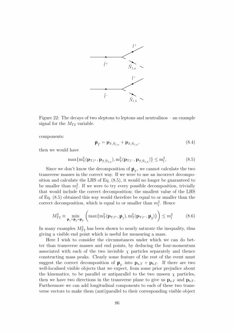
l+

l+

N1,a

l−

N1,b

l−

Figure 22: The decays of two sleptons to leptons and neutralinos – an examplesignal for the MT2 variable.

components:

/pT = pT,N1,a+ pT,N1,a

, (8.4)

then we would have

maxm2T(pT,l+ ,pT,N1,a

),m2T(pT,l− ,pT,N1,b

) ≤ m2l, (8.5)

Since we don’t know the decomposition of /pT , we cannot calculate the twotransverse masses in the correct way. If we were to use an incorrect decompo-sition and calculate the LHS of Eq. (8.5), it would no longer be guaranteed tobe smaller than m2

l. If we were to try every possible decomposition, trivially

that would include the correct decomposition; the smallest value of the LHSof Eq. (8.5) obtained this way would therefore be equal to or smaller than thecorrect decomposition, which is equal to or smaller than m2

l. Hence

M2T2 ≡ min

/p1+/p2

=/pT

(maxm2

T(pT,l+ , /p1),m2

T(pT,l− , /p2))≤ m2

l(8.6)

In many examples M2T2 has been shown to nearly saturate the inequality, thus

giving a visible end point which is useful for measuring a mass.Here I wish to consider the circumstances under which we can do bet-

ter than transverse masses and end points, by deducing the four-momentumassociated with each of the two invisible χ particles separately and thenceconstructing mass peaks. Clearly some feature of the rest of the event mustsuggest the correct decomposition of /pT into pa,T + pb,T . If there are twowell-localised visible objects that we expect, from some prior prejudice aboutthe kinematics, to be parallel or antiparallel to the two unseen χ particles,then we have two directions in the transverse plane to give us pa,T and pb,T .Furthermore we can add longitudinal components to each of these two trans-verse vectors to make them (anti)parallel to their corresponding visible object

86

in three dimensions, giving approximations for pχa,b . If χ is much lighter thanthe particle produced in the hard scattering, i.e. at the start of the decay cas-cade, we can promote pχa,b to massless four-vectors; I will show that combinedwith the four-vectors for the visible decay products, a strong mass peak forthe initial particles can be reconstructed.

8.2 Motivation

Parallel or antiparallel visible and missing energy is not worth considering onlyfor its ease: it can arise in many circumstances. Spin correlations may makeχ particles approximately (anti)parallel to other particles. Two-body decaysof particles P nearly stationary in the lab frame are back-to-back: thereforein 2P → 2χ + 2vis, each χ is nearly antiparallel to one of the ‘vis’. Howeverantiparallelness, unlike parallelness, is not preserved under z-boosts of themother particle, and the z-boost is unknown.

A promising scenario is when each χ is produced together with visibleenergy from the decay of a boosted particle. This will arise whenever (a)directly pair-produced particles are appreciably heavier than whatever theydecay into in the first step of the cascade, and (b) χ are created following twoor more steps. Together these points imply that each of the two sides of theevent (separated according to the mother particle) contains an intermediateparticle which is boosted: the visible object(s) and χ it ultimately decays towill be collimated.

For some examples, consider the quintessential Susy decay of a pair-producedsquark to a hard jet and light neutralino : q → q + N1. There are many rea-sons why we might expect N1 to be unstable, decaying to visible energy and alighter, neutral, collider-stable particle – the latter could be:

• a gravitino G, if Susy breaking is mediated at a low scale, i.e. someform of gauge mediation. A low mediation scale is motivated by elec-troweak naturalness and an automatic solution of the Susy flavour prob-lem. See [192] for a comprehensive list of possible collider signatures.

• a pseudo-Goldstino G′, if more than one hidden sector independentlybreaks Susy and mediates it to the visible sector, as may occur in stringtheory or quiver gauge theories [193, 194]. See [195] for the colliderphenomenology.

• a singlino31 S in the NMSSM. See [123] for the modified collider signals.

• a new photino31 γ′, if the MSSM is extended with one or more extraU(1) gauge symmetries, as is commonly expected to arise from the com-

31In this case the decay is not really q → q + N1 → . . . but q → q + N2 → N1 + . . ., sincenew photinos/singlinos actually mix with the MSSM neutralinos. If N2 is mostly ‘MSSM-like’ (any mixture of Higgsino, wino and bino), and N1 is mostly singlino or a new photino,then direct decay of q to N1 is suppressed relative to the two-step decay.

87

pactification of extra dimensions. See [196] for a discussion of colliderprospects.

In the nomenclature of [196], N1 here is the lightest ordinary supersymmetricparticle (LOSP). All of these examples have some other particle as the trueLSP, and so cosmology allows a charged or coloured Susy particle to be lighterthan N1 and take its place as the LOSP in the cascade q → vis1 + (LOSP)→vis1 + (vis2 + LSP), giving different visible energy.

8.3 The Analysis

I will elaborate on the strategy outlined in Section 8.1 in terms of a concreteexample to allow clearer references to the particles involved in the signal: Iconsider the classic gauge-mediation decay32 2q → 2q+2(N1)→ 2q+2(G+γ).The lightest neutralino is typically expected to be considerably lighter thanthe squarks in this scenario, as renormalisation-group evolution tends to drivesquark masses up and the bino mass down, and the phenomenon of gauginoscreening in the simplest models makes the gauginos much lighter than thescalars (see e.g. [198]). This simple observation gives a powerful handle on thesignal, as yet unexploited: the gravitinos and photons are normally collimated.It is exploited as follows.

1. Uniquely decompose /pT into pa,T + pb,T which are defined to be parallel,in the transverse plane, to the two hardest isolated photons.

2. Promote pa,b;T to three-vectors pa,b by adding the longitudinal compo-nents required to make them parallel to each of the photons in threedimensions.

3. Promote pa,b to massless four-vectors pµa,b = (|pa,b|,pa,b), giving approxi-mations for the two gravitino four-vectors. Adding each of these to thefour-vector of the collinear photon gives massless approximations for thetwo neutralino four-vectors, pµ

N1;a,b.

4. If each neutralino N1;a,b can be paired with the ‘correct’ jet in the eventja,b, then taking the invariant mass of each pair reconstructs the mass ofthe initial squarks: M2

rec;a,b = (pµN1;a,b

+ pµja,b)2

Steps 1-2 above reconstruct the three-momenta of the two neutralinos inthe same way as is done for the two τ in H → 2τ → e±µ∓ /ET with the collinearapproximation of [199]. There, the two τ four-momenta are added together toget the mass of the single mother particle; here the four-momenta of the twoneutralinos are separately added to those of other visible particles in the eventto get the masses of two mother particles – step 4.

Step 4 needs a criterion for the correct way to pair each reconstructedneutralino with one of the jets in the event. The correct jet is considered to be

32A similar final state may arise from Universal Extra Dimensions [197], though semi-invisibly decaying Kaluza-Klein photons from KK quark/gluon decays are not generallyexpected to be boosted; this will be important for my analysis.

88

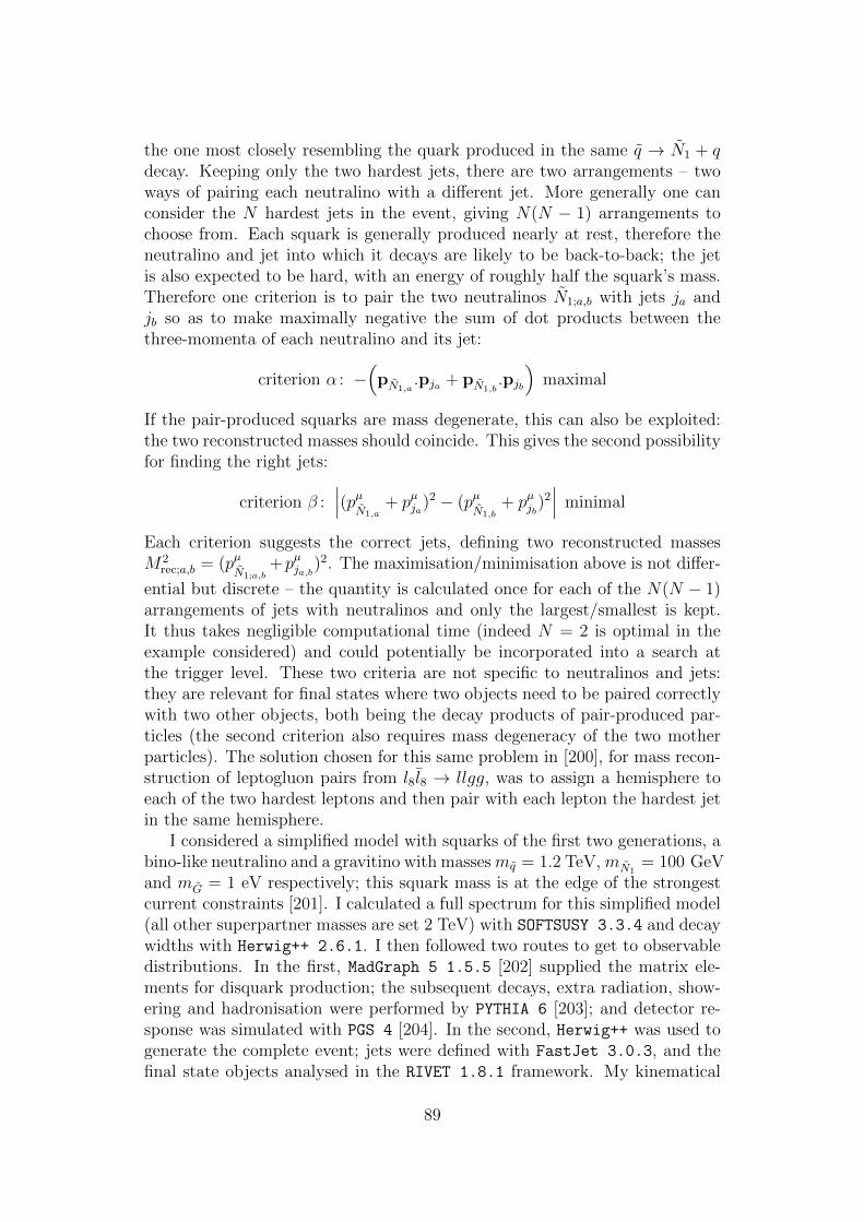
the one most closely resembling the quark produced in the same q → N1 + qdecay. Keeping only the two hardest jets, there are two arrangements – twoways of pairing each neutralino with a different jet. More generally one canconsider the N hardest jets in the event, giving N(N − 1) arrangements tochoose from. Each squark is generally produced nearly at rest, therefore theneutralino and jet into which it decays are likely to be back-to-back; the jetis also expected to be hard, with an energy of roughly half the squark’s mass.Therefore one criterion is to pair the two neutralinos N1;a,b with jets ja andjb so as to make maximally negative the sum of dot products between thethree-momenta of each neutralino and its jet:

criterion α : −(pN1,a

.pja + pN1,b.pjb

)maximal

If the pair-produced squarks are mass degenerate, this can also be exploited:the two reconstructed masses should coincide. This gives the second possibilityfor finding the right jets:

criterion β :∣∣∣(pµ

N1,a+ pµja)

2 − (pµN1,b

+ pµjb)2∣∣∣ minimal

Each criterion suggests the correct jets, defining two reconstructed massesM2

rec;a,b = (pµN1;a,b

+pµja,b)2. The maximisation/minimisation above is not differ-

ential but discrete – the quantity is calculated once for each of the N(N − 1)arrangements of jets with neutralinos and only the largest/smallest is kept.It thus takes negligible computational time (indeed N = 2 is optimal in theexample considered) and could potentially be incorporated into a search atthe trigger level. These two criteria are not specific to neutralinos and jets:they are relevant for final states where two objects need to be paired correctlywith two other objects, both being the decay products of pair-produced par-ticles (the second criterion also requires mass degeneracy of the two motherparticles). The solution chosen for this same problem in [200], for mass recon-struction of leptogluon pairs from l8l8 → llgg, was to assign a hemisphere toeach of the two hardest leptons and then pair with each lepton the hardest jetin the same hemisphere.

I considered a simplified model with squarks of the first two generations, abino-like neutralino and a gravitino with massesmq = 1.2 TeV, mN1

= 100 GeVand mG = 1 eV respectively; this squark mass is at the edge of the strongestcurrent constraints [201]. I calculated a full spectrum for this simplified model(all other superpartner masses are set 2 TeV) with SOFTSUSY 3.3.4 and decaywidths with Herwig++ 2.6.1. I then followed two routes to get to observabledistributions. In the first, MadGraph 5 1.5.5 [202] supplied the matrix ele-ments for disquark production; the subsequent decays, extra radiation, show-ering and hadronisation were performed by PYTHIA 6 [203]; and detector re-sponse was simulated with PGS 4 [204]. In the second, Herwig++ was used togenerate the complete event; jets were defined with FastJet 3.0.3, and thefinal state objects analysed in the RIVET 1.8.1 framework. My kinematical

89

analysis – steps 1-4 with criteria α and β above – was then applied. Code fordoing this, easily generalisable to other final states, can be found at [131].

We chose basic cuts for the analysis as follows:

• At least two jets, clustered using the anti-kt algorithm [205] with sizeparameter 0.4. Jet candidates are required to have pT > 30 GeV and|η| < 4.5.

• At least two isolated photons with pT > 10 GeV. On the MadGraph-PYTHIA route, PGS handles isolation. On the Herwig route, I considereda photon isolated based on total transverse energy deposited inside asurrounding cone (as in the relevant searches [201, 206]), specifically5 GeV in a cone ∆R < 0.4.

• A minimum and maximum azimuthal angular separation between the twohardest isolated photons ε < ∆φγ1γ2 < π − ε with ε = 0.01, since photonswhich are exactly (anti)parallel in the transverse plane do not allow /pTdecomposition.

• The missing energy vector /pT should lie in between the two photons inthe transverse plane (i.e. inside the smaller of the two sectors delim-ited by the two photon directions). This ensures that the event has /pTcorresponding to the ansatz of both gravitinos being parallel (and notantiparallel) to their photons. With this cut the kinematics are alwaysin the ‘trivial zero’ of the MT2 observable (see [207]).

Decomposition of /pT of course requires /ET 6= 0; in practice this is always satis-

fied. I did not cut on /ET – I analysed this particular signal not to optimise theassociated cuts but simply as a demonstration of the mass reconstruction tech-nique. In the present example more than 90% of events have /ET > 100 GeVand so a large requirement could be placed as in existing searches (likewise forthe leading jet and photon which are typically hard in the signal). Note thatwith a requirement for hard photons and /ET there is typically very small back-ground for new physics [208] and the priority is an observable that increasesthe visibility of the signal alone, ideally through a resonance.

Fig. 23 shows the results of the analysis. The initial mass is reconstructedto 10% accuracy for roughly 1

3of events passing the basic cuts. Multiplying

by the Prospino 2 production cross-section and the acceptance – 20 fb × 0.5– one would expect O(100) events inside this peak in 30 fb−1 at 8 TeV.

I obtained an estimate of the expected accuracy of the mass reconstructionin the case of 100 signal events in the following way. Roughly 5000 signalevents were split into samples each containing 100 events. For each samplethe 100 values of the calculated mass were binned, and the mid-point of themodal bin taken to define the position of the peak and thus the reconstructedmass for that sample. The values of the mass determined from each of the∼ 50 samples then define a probability distribution quantifying how well the

90

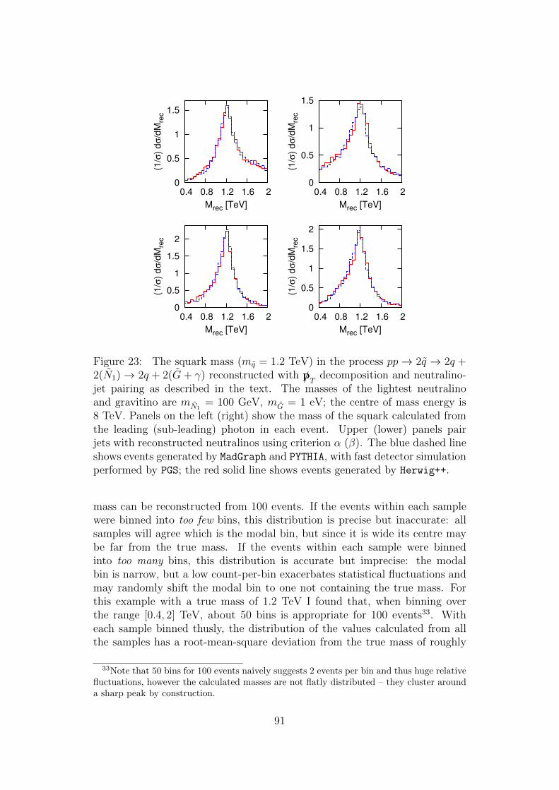
0

0.5

1

1.5

0.4 0.8 1.2 1.6 2

(1/σ

) d

σ/d

Mre

c

Mrec [TeV]

0

0.5

1

1.5

0.4 0.8 1.2 1.6 2

(1/σ

) d

σ/d

Mre

c

Mrec [TeV]

0

0.5

1

1.5

2

0.4 0.8 1.2 1.6 2

(1/σ

) d

σ/d

Mre

c

Mrec [TeV]

0

0.5

1

1.5

2

0.4 0.8 1.2 1.6 2

(1/σ

) d

σ/d

Mre

c

Mrec [TeV]

Figure 23: The squark mass (mq = 1.2 TeV) in the process pp→ 2q → 2q +2(N1)→ 2q + 2(G+ γ) reconstructed with /pT decomposition and neutralino-jet pairing as described in the text. The masses of the lightest neutralinoand gravitino are mN1

= 100 GeV, mG = 1 eV; the centre of mass energy is8 TeV. Panels on the left (right) show the mass of the squark calculated fromthe leading (sub-leading) photon in each event. Upper (lower) panels pairjets with reconstructed neutralinos using criterion α (β). The blue dashed lineshows events generated by MadGraph and PYTHIA, with fast detector simulationperformed by PGS; the red solid line shows events generated by Herwig++.

mass can be reconstructed from 100 events. If the events within each samplewere binned into too few bins, this distribution is precise but inaccurate: allsamples will agree which is the modal bin, but since it is wide its centre maybe far from the true mass. If the events within each sample were binnedinto too many bins, this distribution is accurate but imprecise: the modalbin is narrow, but a low count-per-bin exacerbates statistical fluctuations andmay randomly shift the modal bin to one not containing the true mass. Forthis example with a true mass of 1.2 TeV I found that, when binning overthe range [0.4, 2] TeV, about 50 bins is appropriate for 100 events33. Witheach sample binned thusly, the distribution of the values calculated from allthe samples has a root-mean-square deviation from the true mass of roughly

33Note that 50 bins for 100 events naively suggests 2 events per bin and thus huge relativefluctuations, however the calculated masses are not flatly distributed – they cluster arounda sharp peak by construction.

91

60 GeV: determination at the 5% level. To put this number (very) roughly incontext, the ATLAS Collaboration’s Technical Design Report [169] consideredthe signal 2 × (q → χ0

2q → llq → χ01llq) arising as part of a CMSSM (not

simplified) model. Using kinematic edges,the squark mass could be determinedto within 3% with O(106) events before cuts; c.f. 5% with only 200 eventsbefore cuts (100 events after cuts) for the signal and method considered here.

As my analysis makes use of hard jets arising from the decay of signalparticles, it could in principle be affected by the (higher order) production ofadditional jets in the hard scattering. To investigate this I simulated 2q and2q+1jet production and combined these consistently into a single sample usingthe MLM matching procedure [209]. The reconstructed mass distributions areessentially identical to those of simple 2q production shown in Fig. 23, whichfollows from the fact that my method is designed to find the two jets that lookmost like they have been produced by the decay of the squarks, and discardother jets.

Criterion α can also reconstruct the masses of pair-produced non-degenerateparticles. In Fig. 24 it is used to analyse the same signal as previously butnow with one squark from the first two generations having mass 1.1 TeV andthe other seven having mass 1.4 TeV. This unequal splitting is chosen to havelarge cross-sections for the production of two squarks of different mass (fourlighter squarks and four heavier would merely result in a dominant produc-tion of two of the lighter four); nevertheless production of two squarks of thesame mass still has non-zero cross-section. Thus the distribution of the larger(smaller) of the two masses calculated for each event peaks strongly at 1.4 TeV(1.1 TeV) and weakly at 1.1 TeV (1.4 TeV), with the weak peak resulting frompair-produced degenerate squarks.

8.4 Discussion

The final state of the example considered has two jets and two pairs of roughlycollinear photons and gravitinos. The jet could be replaced by any other visi-ble particle – ‘vis1’ – the photon too – ‘vis2’ – and the gravitino by anythinginvisible, χ: I show this general topology in Fig. 25. Provided there are twosemi-invisible decays which are boosted (or forced into (anti)parallel behaviourby spin correlations) the same analysis presented here should in theory havesome potential for mass reconstruction. Of course if vis1 and vis2 are objectsless clean experimentally than light-flavour jets and photons, such as b quarksor even combinations of particles, the procedure will be more difficult in prac-tice. Searches for mass peaks in the manner presented, considering variousdifferent particle types for vis1,2, could discover expected or unexpected reso-nances. Below, I outline how the method might be adapted as the topology isdistorted and generalised further.

92

0

0.2

0.4

0.6

0.8

1

1.2

1.4

0.5 0.8 1.1 1.4 1.7 2

(1/σ

) d

σ/d

Mre

c

Mrec [TeV]

Figure 24: As Fig. 23 but with one squark from the first two generationshaving mass 1.1 TeV and the other seven having mass 1.4 TeV. The solid red(dashed blue) line shows the smaller (larger) of the two masses reconstructedin each event. Only criterion α for jet-neutralino pairing is used. Events aregenerated with Herwig++.

vis1

vis1

χ

χ

vis2

vis2

Figure 25: The topology I consider: pair-produced particles each decay into avisible Standard Model particle vis1 and a much lighter particle, which is thusboosted; this decays semi-invisibly into vis2 and χ.

A Less Boosted Intermediate. Collinearity of χ and vis2 relies on their com-mon mother particle being boosted; as it becomes less boosted they becomeless collinear. I show this effect, and the decreasing sharpness of the mass re-construction that results, in Fig. 26 for my previous gauge-mediation example.mN1

is increased from 100 to 400 GeV for constant mq = 1.2 TeV. If N1 is madeheavier still, e.g. mN1

/mq → 1, the increasingly lethargic neutralino gives aless collimated photon-gravitino pair; indeed the two are increasingly back-to-back, and most events fail to meet the requirement that /pT be in between thetwo photons.

More Decays Of The Intermediate. If vis2 is several particles instead ofthe single photon γ I considered, e.g. a lepton pair from a boosted Ni →

93

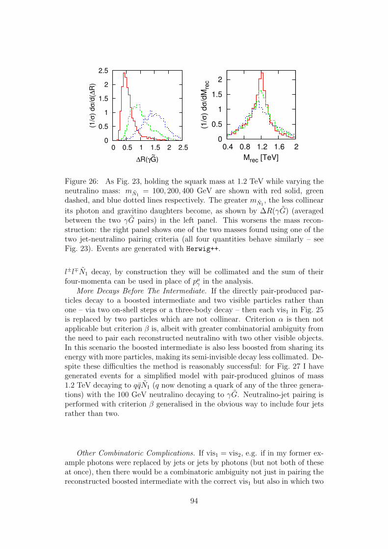
0

0.5

1

1.5

2

2.5

0 0.5 1 1.5 2 2.5

(1/σ

) d

σ/d

(∆R

)

∆R(γG~

)

0

0.5

1

1.5

2

0.4 0.8 1.2 1.6 2

(1/σ

) d

σ/d

Mre

c

Mrec [TeV]

Figure 26: As Fig. 23, holding the squark mass at 1.2 TeV while varying theneutralino mass: mN1

= 100, 200, 400 GeV are shown with red solid, greendashed, and blue dotted lines respectively. The greater mN1

, the less collinear

its photon and gravitino daughters become, as shown by ∆R(γG) (averagedbetween the two γG pairs) in the left panel. This worsens the mass recon-struction: the right panel shows one of the two masses found using one of thetwo jet-neutralino pairing criteria (all four quantities behave similarly – seeFig. 23). Events are generated with Herwig++.

l±l∓N1 decay, by construction they will be collimated and the sum of theirfour-momenta can be used in place of pµγ in the analysis.

More Decays Before The Intermediate. If the directly pair-produced par-ticles decay to a boosted intermediate and two visible particles rather thanone – via two on-shell steps or a three-body decay – then each vis1 in Fig. 25is replaced by two particles which are not collinear. Criterion α is then notapplicable but criterion β is, albeit with greater combinatorial ambiguity fromthe need to pair each reconstructed neutralino with two other visible objects.In this scenario the boosted intermediate is also less boosted from sharing itsenergy with more particles, making its semi-invisible decay less collimated. De-spite these difficulties the method is reasonably successful: for Fig. 27 I havegenerated events for a simplified model with pair-produced gluinos of mass1.2 TeV decaying to qqN1 (q now denoting a quark of any of the three genera-tions) with the 100 GeV neutralino decaying to γG. Neutralino-jet pairing isperformed with criterion β generalised in the obvious way to include four jetsrather than two.

Other Combinatoric Complications. If vis1 = vis2, e.g. if in my former ex-ample photons were replaced by jets or jets by photons (but not both of theseat once), then there would be a combinatoric ambiguity not just in pairing thereconstructed boosted intermediate with the correct vis1 but also in which two

94

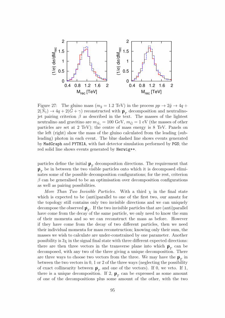
0

0.5

1

1.5

2

0.4 0.8 1.2 1.6 2

(1/σ

) d

σ/d

Mre

c

Mrec [TeV]

0

0.5

1

1.5

2

0.4 0.8 1.2 1.6 2

(1/σ

) d

σ/d

Mre

c

Mrec [TeV]

Figure 27: The gluino mass (mg = 1.2 TeV) in the process pp → 2g → 4q +2(N1)→ 4q + 2(G+ γ) reconstructed with /pT decomposition and neutralino-jet pairing criterion β as described in the text. The masses of the lightestneutralino and gravitino are mN1

= 100 GeV, mG = 1 eV (the masses of otherparticles are set at 2 TeV); the centre of mass energy is 8 TeV. Panels onthe left (right) show the mass of the gluino calculated from the leading (sub-leading) photon in each event. The blue dashed line shows events generatedby MadGraph and PYTHIA, with fast detector simulation performed by PGS; thered solid line shows events generated by Herwig++.

particles define the initial /pT decomposition directions. The requirement that

/pT be in between the two visible particles onto which it is decomposed elimi-nates some of the possible decomposition configurations; for the rest, criterionβ can be generalised to be an optimisation over decomposition configurationsas well as pairing possibilities.

More Than Two Invisible Particles. With a third χ in the final statewhich is expected to be (anti)parallel to one of the first two, our ansatz forthe topology still contains only two invisible directions and we can uniquelydecompose the observed /pT . If the two invisible particles that are (anti)parallelhave come from the decay of the same particle, we only need to know the sumof their momenta and so we can reconstruct the mass as before. Howeverif they have come from the decay of two different particles, then we needtheir individual momenta for mass reconstruction; knowing only their sum, themasses we wish to calculate are under-constrained by one parameter. Anotherpossibility is 3χ in the signal final state with three different expected directions:there are then three vectors in the transverse plane into which /pT can bedecomposed, with any two of the three giving a unique decomposition. Thereare three ways to choose two vectors from the three. We may have the /pT inbetween the two vectors in 0, 1 or 2 of the three ways (neglecting the possibilityof exact collinearity between /pT and one of the vectors). If 0, we veto. If 1,there is a unique decomposition. If 2, /pT can be expressed as some amountof one of the decompositions plus some amount of the other, with the two

95

coefficients constrained to sum to unity: the masses we wish to calculate areunder-constrained by one parameter. One response, not physically motivated,would be to veto. Another possibility could be to set the two coefficients basedon some other prejudice about the kinematics, such as making an intermediateparticle of known mass maximally on-shell. Which of these three cases (0, 1or 2 of the possible decompositions being acceptable) we have will vary on anevent by event basis.

96

Appendix A The Higgs As A Pseudo-Nambu-

Goldstone Boson (‘Little Higgs’)

See [210] for a review and original references, also [211, 212]. When a continu-ous global symmetry G is spontaneously broken to a subgroup H, Goldstone’sTheorem tells us that dim(G)− dim(H) Nambu-Goldstone bosons (NGBs) re-sult. (Mild explicit breaking, i.e. from small terms in the Lagrangian, resultsinstead in pseudo-NGBs (pNGBs), which are light but not massless.) If Gcontained a subgroup F which was gauged, and which gets broken down toI ≡ F ∩ H, then dim(F) − dim(I) of the NGBs are eaten to give masses toall of the bosons associated with the generators of the (entirely broken) F/Icoset. This leaves (dim(G) − dim(H)) − (dim(F) − dim(I)) NGBs. I shouldbe (or contain) the Standard Model SU(2)L×U(1)Y ; and amongst the NGBswe want there to be (a) three degrees of freedom that will ultimately be eatenby the W and Z bosons, as in the Standard Model, but also (b) a degree offreedom corresponding to the Higgs. In this way we have made the Higgs light;unfortunately we have made it massless, however one thing at a time.

Now let us add a term to the Lagrangian which involves the Higgs, respectsH, but breaks G. The Higgs is now a pNGB rather than a NGB. However werun straight back into the hierarchy problem: through such a term we havea one-loop quadratic divergence, previously forced to be zero by virtue of thesymmetry only being broken at the level of the vacuum and not the Lagrangian.So instead of explicit breaking with one term, we can use two: we add to theLagrangian λ1L1 + λ2L2 which only break G to H when they are present to-gether, a phenomenon we call collective symmetry breaking. With only oneof the terms, there is a sufficient amount of symmetry broken only sponta-neously and not explicitly that the Higgs is still a NGB. With both terms it isa pNGB, and we do have quadratic divergences as we must with explicit sym-metry breaking, but only at two loops: δm2

H ∼ (λ1/16π2)(λ2/16π2)Λ2, sinceby construction all corrections identically vanish when one coupling vanisheseven if the other does not. The one-loop divergence due to the top loop iscancelled by a similar diagram containing in the loop a fermionic partner ofthe top – a partner which is a necessary part of such a setup.

The expected cutoff for naturalness is then postponed to 10 TeV ratherthan 1 TeV. We must then ask what comes next. Perhaps nothing moreuntil the Planck scale, if our global symmetry G was broken spontaneously bya weakly coupled scalar whose vacuum expectation value v little Higgs is, whilelarger than vSM = 174 GeV, still mysteriously smaller than MP . There couldbe a tower of stacked little Higgs models – each symmetry-breaking scalar beingthe pNGB of a different symmetry at higher scales – as discussed in [213]. Inthis case, while the scalar at the bottom of the stack (which plays the role ofthe Standard Model Higgs) encounters the quadratically divergent correctionat progressively higher orders, increasing numerical factors multiplying theterm do not allow escape from the Hierarchy problem. Alternatively one of

97

the three traditional natural theories may come into play above this cutoff –extra dimensions, compositeness, or Susy.

98

Appendix B Optimal Naturalness Beyond Lead-

ing Log δm2Hu

The leading log expression for δm2Hu

is obtained by ignoring the scale depen-dence of At and MS; to do better we can integrate At and MS over their varyinghigher-scale values. First consider the running of At and MS with arbitraryself and mutual couplings, as well couplings to other particles:

d

dt

(M2

S(t)A2t (t)

)=

(a(t) b(t)

0 c(t)

)(M2

S(t)A2t (t)

)+ other running soft-mass terms

(B.1)

∴

(M2

S(t)A2t (t)

)=

(d(t) e(t)

0 f(t)

)(M2

S(0)A2t (0)

)+ other high-scale soft-mass terms,

(B.2)

where a, b, c are running couplings and d, e, f are related to the former by in-tegration, and the lower-left entry of the matrix must vanish since At appearsin the Lagrangian, not A2

t . Note that if the other soft-mass parameters them-selves run due to At and MS, this feeds back into Eq. (B.2) as corrections tothe coefficients d, e, f suppressed by an extra loop factor, which could have animpact but I will neglect this for simplicity. Integrating the m2

Hubeta func-

tion (2.2), keeping just the stop-sector terms as before but now including theirscale dependence (and that of the top Yukawa) as in (B.2), we have

δm2Hu(t) = 3

8π2

(2M2

S(0)

∫ t′=t

t′=0

y2t (t′)d(t′) dt′+

A2t (0)

∫ t′=t

t′=0

y2t (t′)(2e(t′) + f(t′)) dt′

)+ other high-scale soft-mass terms (B.3)

For Lagrange constrained optimisation, Eq. (2.5), we must differentiate δm2Hu

and δm2h with respect to A2

t and M2S. One can either invert Eq. (B.2) and

substitute into Eq. (B.3) to obtain δm2Hu

instead as a function of the low-scalestop parameters, or all derivatives can be taken with respect to the high-scalestop parameters (using the chain rule for δm2

h, whose arguments should beevaluated at the low scale). Both approaches give the same result, as theymust:

f(t)

(2

∫ t′=t

t′=0

y2t (t′) d(t′) dt′ + d(t)y2

t (t)

(1 +

A2t (t)

2M2S(t)

))∂(δm2

h)

∂A2t

=(d(t)

∫ t′=t

t′=0

y2t (t′)(2e(t′) + f(t′)) dt′ − 2e(t)

∫ t′=t

t′=0

y2t (t′) d(t′) dt′

)∂(δm2

h)

∂M2S

(B.4)

99

The leading log relation is recovered for (d(t), e(t), f(t)) = (1, 0, 1), yt(t) = yt.So what are these functions d(t), e(t), f(t) in the MSSM? Expressions for theone-loop running parameters can be written down when all Yukawa couplingsexcept that of the top are set to zero [214, 215, 216]. yt(t) and At(t) donot require numerical integration if one also sets the U(1) and SU(2) gaugecouplings to zero: one finds

y2t (t) = y2

t (0) ξ−16/9(t)G−1(t; −169

) (B.5)

At(t) = G−1(t; −169

)

[At(0) +

16

9M3(0)

(G(t; −16

9)ξ−1(t)− G(t; −25

9))]

(B.6)

where ξ(t) = 1 +3

2πα3(0)t

G(t;n) = 1− 3

4π2y2t (0)

∫ t

0

dt′ ξn(t′)

From (B.6) we can read off that f(t) = G−1(t; −169

). In this same scheme for ex-tracting running parameters, the stop mass necessarily involves numerical inte-gration. However RG-induced splitting of the stop from the lighter-generationup-type quarks is typically small (and if not the model is necessarily unnatural,as mentioned in Section 1.4), so that the running stop is well approximated byits high-scale value plus the gluino-induced term, the latter easily obtained byintegrating the one-loop running gluino mass:

M2S(t) = M2

S(0) +8

9M2

3 (0)

(α2

3(t)

α23(0)− 1

)(B.7)

This gives d(t) = 1, e(t) = 0. Eq. (B.4) is then

2G−1(t; −169

)

(∫ t′=t

t′=0

(ξ−16/9(t′)G−1(t′; −16

9)

)dt′

+ξ−16/9(t)G−1(t; −169

)

(1 +

A2t (t)

2M2S(t)

))∂(δm2

h)

∂A2t

=∫ t′=t

t′=0

(ξ−16/9(t′)G−2(t′; −16

9)

)dt′

∂(δm2h)

∂M2S

(B.8)

The integrals can be done analytically and the resulting root, xnatural, found;I do not plot it as it is essentially indistinguishable from the one shown inFig. 3, even for very high mediation scales Λ ∼ 1016 GeV. Thus my attempt atan approximate RG improvement of δm2

Hu(resumming all the logs that come

with appreciable coupling constant factors) makes no difference to the resultobtained from the leading log expression.

An alternative approach to this approximate RG improvement would beto work consistently at Next-to-Leading-Log NLL order for δm2

Hu. Barbieri-

Giudice fine-tuning measures are given at NLL in [68], from which one can

100

extract the dependence of δm2Hu

on any trilinear mixing term or sfermionmass-squared via

δm2Hu(Ai) =

∫ (M2

Z

2AiZAi |tanβ→∞

)dAi (B.9)

δm2Hu(m2

f) =

M2Z

4Zmf

∣∣∣tanβ→∞

(B.10)

where Zpi ≡∂(logM2

Z)

∂(log pi)

Note that δm2Hu

and m2f

both having mass dimension 2 results in Zmf ∝ mf ,

giving the simpler expression (B.10). ZAi however can contain further mass-scales beyond Ai; indeed for the stop, ZAt contains terms with M1, M3 and Ab.In other words, at NLL δm2

Hudepends on At not only through an A2

t term butalso through terms AtM1, AtM3 and AtAb. In the spirit of connecting δm2

Hu

and the Higgs mass to the stop sector in isolation, I will not explore this effecthere.

101

Appendix C Brazil-Band Plots For Dummies

Brazil-band plots are used to present exclusion limits for the existence of newparticles whose decays are uniquely determined as a function of their mass34.Before any data is collected, one can calculate the expected σ95%CL /σsignal forany given mass m of the new particle. σsignal is defined as in Section 6.1 (σ un-fortunately also denotes uncertainty/error in predictions and measurements).I will refer interchangeably to numbers of events N and cross-sections σ asthey differ only by a factor of the integrated luminosity L, through N = σL.σx%CL is the cross-section excluded at x% confidence level: roughly, the signalcross-section for which the probability of signal plus background fluctuating aslow as the observed value is less than (100− x)% (a statement to be clarifiedshortly). x = 95 is common in particle physics. The expected σ95%CL refers tothe limit that would be set if the number of events observed coincided withthe number of events expected from the background alone.

Let’s develop a feel for how the expected σ95%CL /σsignal will behave. Wepredict a certain number of events from the background Nb and from thesignal Ns, and there is uncertainty in both predictions. Statistical error, be-cause both follow from probability distributions. Systematic error, becausethe experiment may consistently mismeasure something, and the theoreticalestimate is made to a finite order in perturbation theory and so is consis-tently a little off. Now, if the predicted number of signal events is roughlyless than the combined uncertainty in the background and in the signal, thenobserving only the expected number of background events Nb and no more stillwouldn’t allow you to sensibly exclude the presence of signal – it’s sufficientlysmall as to be compatible with Nb events, within the errors. In this case wehave σ95%CL /σsignal > 1. On the other hand if the predicted number of signalevents is roughly greater than the combined uncertainty, then the presence ofthe signal ought to be visible above the background; in this case observingonly Nb events and no more would be compelling evidence for no signal, givingan exclusion: σ95%CL /σsignal < 1.

Also shown in Brazil-band plots are the ±σ,±2σ uncertainties in the ex-pected exclusion – the edges of the green and yellow regions respectively.Where do these come from? We have a probability distribution for the numberof background events (with an expected value Nb). For each possible numberof observed events, we would set a different limit, because more (less) eventsmakes the signal look more (less) likely to exist. Calculating the resultinglimit as a function of events then lets us transform the probability distribu-tion for number of background events into a probability distribution for theresulting limit. I am now in a position to clarify a previous statement – thatthe expected limit the limit that would result from observing Nb events – morespecifically it is the median of the distribution I have just described. The ±σ

34If n extra parameters were needed to fully specify the decays, n extra dimensions wouldbe needed to plot the exclusion results. The Higgs boson of the Standard Model and theW ′, Z ′ of the Sequential Standard Model, for example, all handily have n = 0.

102

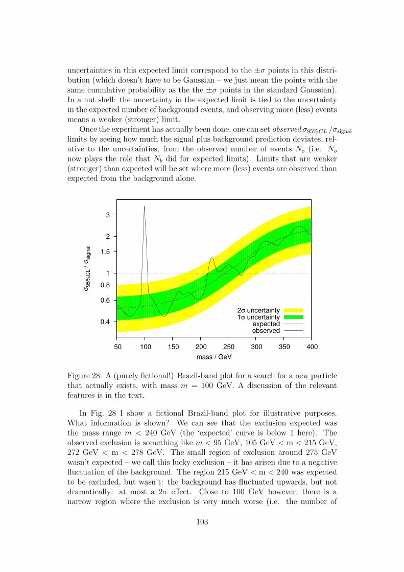
uncertainties in this expected limit correspond to the ±σ points in this distri-bution (which doesn’t have to be Gaussian – we just mean the points with thesame cumulative probability as the the ±σ points in the standard Gaussian).In a nut shell: the uncertainty in the expected limit is tied to the uncertaintyin the expected number of background events, and observing more (less) eventsmeans a weaker (stronger) limit.

Once the experiment has actually been done, one can set observed σ95%CL /σsignal

limits by seeing how much the signal plus background prediction deviates, rel-ative to the uncertainties, from the observed number of events No (i.e. No

now plays the role that Nb did for expected limits). Limits that are weaker(stronger) than expected will be set where more (less) events are observed thanexpected from the background alone.

0.4

0.6

0.8

1

1.5

2

3

50 100 150 200 250 300 350 400

σ9

5%

CL /

σsig

na

l

mass / GeV

2σ uncertainty1σ uncertainty

expectedobserved

Figure 28: A (purely fictional!) Brazil-band plot for a search for a new particlethat actually exists, with mass m = 100 GeV. A discussion of the relevantfeatures is in the text.

In Fig. 28 I show a fictional Brazil-band plot for illustrative purposes.What information is shown? We can see that the exclusion expected wasthe mass range m < 240 GeV (the ‘expected’ curve is below 1 here). Theobserved exclusion is something like m < 95 GeV, 105 GeV < m < 215 GeV,272 GeV < m < 278 GeV. The small region of exclusion around 275 GeVwasn’t expected – we call this lucky exclusion – it has arisen due to a negativefluctuation of the background. The region 215 GeV < m < 240 was expectedto be excluded, but wasn’t: the background has fluctuated upwards, but notdramatically: at most a 2σ effect. Close to 100 GeV however, there is anarrow region where the exclusion is very much worse (i.e. the number of

103

events observed is much higher) than expected. This is strong evidence for anew particle of roughly that mass! The width of the excess gets contributionsfrom the mass resolution and bin width of the relevant search channel, and theparticle’s own fundamental width; being dominated by whichever is largest.All three of these factors will smear out an otherwise delta-function peak inthe invariant mass distribution of the particle’s decay products. Note thatall the way along the plot the exclusion (and by implication the background)fluctuates above and below what was expected, but it’s only in places wherethe expected value of σ95%CL /σsignal is one side of 1 and the observed valueis on the other that the result of exclusion or non-exclusion deviates fromexpectation.

For completeness I’ll mention ‘blue-band’ or signal strength plots, whichbecome useful when we have not just exclusion but also a (tentative) discovery.The signal strength, often denoted µ, is the factor by which the signal cross-section should be multiplied for best agreement with the data. There are anumber of points worth noting about µ.

• An exact expression for µ, based on maximising the likelihood functionfor obtaining all of the observed data, would be complicated. Howeverfor a given mass value m that predicts Ns signal events, with Nb eventsexpected from the background and No events observed (with Ns, Nb andNo referring to events in the vicinity of the signal at m, not elsewhere),one can think of µ as being given by No ≈ Nb + µNs.

• µ = 0 ⇔ perfect description of the data by the background alone. µ =1⇔ perfect description of the data by the background plus signal, withno modification of the signal. Of course for either of these two statementsto be meaningful requires small error bars on µ: σµ < 1 or preferably 1.

• While physical cross-sections are positive semi-definite, µ is negativewhenever less events are observed than predicted for the backgroundalone.

• How does µ relate to the Brazil-band plot? The approximate relationNo ≈ Nb + µNs shows that µ is positive (negative) where more (less)events are observed than expected from the background alone. Therefore

Sign(µ) ≈ Sign

(σ95%CL,observed

σsignal

− σ95%CL,expected

σsignal

), (C.1)

or in words, the sign of µ generally follows the sign of the fluctuation ofthe observed limit from what was expected. Knowing that a given massvalue is not excluded, the corresponding µ can in principle take any value.All positive values are possible since the lack of exclusion could be dueto the presence of a real signal, but with arbitrarily modified strength.All negative values of possible since we might be dealing with a deficit of

104

observed events, but an insignificant deficit relative to our uncertainties.Knowing that a given mass value is excluded, the corresponding µ mustbe less than one, since exclusion refers specifically to the µ = 1 case.Therefore we can make one inference going the other way, from blueband to Brazil band: µ ≥ 1 points are not excluded, µ < 1 points mayor may not be. But it’s best just to take the relevant information fromeach respective plot.

Earlier I said that σ95%CL is the signal cross-section for which the probabil-ity of signal plus background fluctuating as low as the observed value, denotedps+b, is less than 5%. However sometimes by chance, No will fluctuate so lowthat even the background-only hypothesis Hb is a poor description of the data.If this is the case, we should consider the signal plus background hypothe-sis Hs+b excluded only if does a much worse job even than Hb at describingthe data. If it is merely equally poor, the data isn’t helping us to distinguishwhether or not there is any signal. Considering the signal to be excluded in thiscase based on ps+b < 0.05 would be a spurious exclusion, and we can protectourselves against this using the CLs method [217, 218]. CLs ≡ ps+b/(1 − pb),with pb the probability of the background alone contributing at least as manyevents as observed; and we now require CLs < 0.05 instead of ps+b < 0.05.Then when Hb and Hs+b do comparably poor jobs at describing a deficit inevents, ps+b ∼ 1− pb and CLs remains greater than 5%. By construction, theCLs method prevents cross-section limits becoming too small, and so the ±σuncertainty in the expected limit will be asymmetric – smaller in the negativedirection than in the positive direction. This sometimes has the curious effectof counterbalancing the asymmetry induced by plotting σ95%CL /σsignal on alogarithmic scale!35

I mentioned that the width of the strong excess in Fig. 28 is given by acombination of the experimental mass resolution, bin width, and the hypoth-esised particle’s width. Indeed the width of any excess or deficit in the plot,significant or not, should be governed by this same combination; call it ∆m.(Note that ∆m may change with m: the physical width can obviously change,and particularly if we combine different search channels in one plot the massresolution and bin width can jump whenever we pass between regions wheredifferent search channels are most sensitive.) As an example, consider a deficitof events observed in the bin containing the mass value M , so that we havestronger constraints on the particle near m ∼ M , giving a dip in the Brazil-band plot at that point. Since the mass of the decay products will be smearedout by ∆m, all points in the mass range |m −M | . ∆m will feel this localstrong constraint, and the dip in the plot will be ∼∆m wide. The same logicapplies for a local excess giving a peak in the plot ∼∆m wide. (Note thatin making Fig. 28 I was not careful about giving the random fluctuations areasonably consistent width.) Fluctuations a bit broader than ∆m will occur

35Thanks to the other participants of the Cargese International School 2012 for posingthis question and to Glen Cowan for answering it!

105

when two (or more) bins close to each other both have deficits or both haveexcesses. Thus the broader the fluctuation relative to ∆m, the less likely it isthat the source is a statistical fluctuation: overall we expect correlations overscales ∼ ∆m. For much larger correlations / broader fluctuations, we are likelyto conclude that the background was inaccurately modelled in that mass range,so that the (background only) events we observed were consistently above orbelow the prediction.

106

Appendix D Cuts For The ATLAS Collabo-

ration’s 1.04 fb−1 Search For Susy

With Jets And Missing Energy

The cuts that were chosen for this analysis [177], and which I reproduced inthe RIVET analysis ATLAS 2011 S9212183 are as follows:

• Jet candidates are reconstructed using the anti-kt jet clustering algo-rithm [205] with a distance parameter of 0.4. Candidates withpT < 20 GeV are discarded.

• Electron (muon) candidates are required to have pT > 20 GeV (10 GeV)and |η| < 2.47 (2.4).

• Jet candidates within a distance ∆R = 0.2 of an electron candidate arediscarded, then electron or muon candidates within a distance ∆R = 0.4of surviving jet candidates are discarded. Next, all jet candidates with|η| > 2.8 are discarded.

• The event is vetoed if there are any electrons or muons with pT > 20 GeV.

• Thereafter five separate search channels are defined, each with its ownrequirements on hadronic activity, meff and /ET/meff , summarised inTable 6. The effective mass meff is calculated as the sum of /ET andthe pT of the two, three or four hardest jets used to define the searchchannel. In the high mass channel, all jets with pT > 40 GeV are used tocompute the meff value used in the final cut. The ∆φ cut is only appliedup to the third leading jet.

Signal Region ≥ 2-jet ≥ 3-jet ≥ 4-jet High mass

/ET > 130 > 130 > 130 > 130Leading jet pT > 130 > 130 > 130 > 130Second jet pT > 40 > 40 > 40 > 80Third jet pT – > 40 > 40 > 80Fourth jet pT – – > 40 > 80∆φ(jet, /pT )min > 0.4 > 0.4 > 0.4 > 0.4/ET/meff > 0.3 > 0.25 > 0.25 > 0.2meff > 1000 > 1000 > 500/1000 > 1100

Table 6: Cuts for the five search channels in the ATLAS Collaboration’s1.04 fb−1 jets+/ET search for Susy, lifted straight from the source [177] (meff ,/ET and pT in GeV).

107

References

[1] G. ’t Hooft, NATO Adv.Study Inst.Ser.B Phys. 59, 135 (1980).

[2] R. Kaul, Naturalness and electro-weak symmetry breaking, http://

theory.tifr.res.in/stringslhc/talks/naturalness-ewsb.pdf.

[3] L. Randall and R. Sundrum, Phys.Rev.Lett. 83, 3370 (1999), hep-ph/9905221.

[4] R. Contino, Y. Nomura, and A. Pomarol, Nucl.Phys. B671, 148 (2003),hep-ph/0306259.

[5] K. Agashe, R. Contino, and A. Pomarol, Nucl.Phys. B719, 165 (2005),hep-ph/0412089.

[6] S. P. Martin, (1997), hep-ph/9709356.

[7] M. Drees, (1996), hep-ph/9611409.

[8] A. Signer, J.Phys. G36, 073002 (2009), 0905.4630.

[9] S. Coleman and J. Mandula, Phys. Rev. 159, 1251 (1967).

[10] R. Haag, J. T. Lopuszanski, and M. Sohnius, Nuclear Physics B 88, 257(1975).

[11] D. Boulware, S. Deser, and J. Kay, Physica A: Statistical Mechanics andits Applications 96, 141 (1979).

[12] T.-P. Hack and M. Makedonski, Phys.Lett. B718, 1465 (2013),1106.6327.

[13] G. Bertone, D. Hooper, and J. Silk, Phys.Rept. 405, 279 (2005), hep-ph/0404175.

[14] R. Peccei and H. R. Quinn, Phys.Rev.Lett. 38, 1440 (1977).

[15] R. Peccei and H. R. Quinn, Phys.Rev. D16, 1791 (1977).

[16] ATLAS Collaboration, G. Aad et al., Phys.Lett. B716, 1 (2012),1207.7214.

[17] CMS Collaboration, S. Chatrchyan et al., Phys.Lett. B716, 30 (2012),1207.7235.

[18] G. F. Giudice and A. Strumia, Nucl.Phys. B858, 63 (2012), 1108.6077.

[19] G. F. Giudice, M. A. Luty, H. Murayama, and R. Rattazzi, JHEP 9812,027 (1998), hep-ph/9810442.

108

[20] J. D. Wells, (2003), hep-ph/0306127.

[21] N. Arkani-Hamed and S. Dimopoulos, JHEP 0506, 073 (2005), hep-th/0405159.

[22] G. Giudice and A. Romanino, Nucl.Phys. B699, 65 (2004), hep-ph/0406088.

[23] P. J. Fox et al., (2005), hep-th/0503249.

[24] P. Fayet and J. Iliopoulos, Phys.Lett. B51, 461 (1974).

[25] S. Dimopoulos and H. Georgi, Nuclear Physics B 193, 150 (1981).

[26] N. Sakai, Zeitschrift fr Physik C Particles and Fields 11, 153 (1981).

[27] P. Bechtle et al., (2012), 1211.1955.

[28] A. Arbey, M. Battaglia, A. Djouadi, and F. Mahmoudi, (2012),1211.4004.

[29] P. Bechtle et al., (2013), 1301.2345.

[30] S. Ferrara, L. Girardello, and F. Palumbo, Phys. Rev. D 20, 403 (1979).

[31] R. Barbieri and G. Giudice, Nuclear Physics B 306, 63 (1988).

[32] B. Allanach and M. Parker, (2012), 1211.3231.

[33] R. Kitano and Y. Nomura, Phys.Lett. B631, 58 (2005), hep-ph/0509039.

[34] M. Papucci, J. T. Ruderman, and A. Weiler, JHEP 1209, 035 (2012),1110.6926.

[35] CERN Report No. ATLAS-CONF-2012-109, 2012 (unpublished).

[36] H. K. Dreiner, M. Kramer, and J. Tattersall, Europhys.Lett. 99, 61001(2012), 1207.1613.

[37] G. Belanger, M. Heikinheimo, and V. Sanz, JHEP 1208, 151 (2012),1205.1463.

[38] B. Allanach and B. Gripaios, JHEP 1205, 062 (2012), 1202.6616.

[39] S. E. Hedri, A. Hook, M. Jankowiak, and J. G. Wacker, (2013),1302.1870.

[40] D. Curtin, R. Essig, and B. Shuve, (2012), 1210.5523.

[41] J. Thaler and K. Van Tilburg, JHEP 1103, 015 (2011), 1011.2268.

109

[42] J. Gallicchio and M. D. Schwartz, Phys.Rev.Lett. 105, 022001 (2010),1001.5027.

[43] G. D. Kribs and A. Martin, Phys.Rev. D85, 115014 (2012), 1203.4821.

[44] CMS Collaboration, S. Chatrchyan et al., (2013), 1303.2985.

[45] CERN Report No. CMS-PAS-SUS-12-023, 2012 (unpublished).

[46] CERN Report No. ATLAS-CONF-2013-037, 2013 (unpublished).

[47] CERN Report No. ATLAS-CONF-2012-166, 2012 (unpublished).

[48] S. Dimopoulos and G. Giudice, Phys.Lett. B357, 573 (1995), hep-ph/9507282.

[49] A. G. Cohen, D. Kaplan, and A. Nelson, Phys.Lett. B388, 588 (1996),hep-ph/9607394.

[50] C. Brust, A. Katz, S. Lawrence, and R. Sundrum, JHEP 1203, 103(2012).

[51] N. Craig, M. McCullough, and J. Thaler, JHEP 1206, 046 (2012),1203.1622.

[52] N. Craig, S. Dimopoulos, and T. Gherghetta, JHEP 1204, 116 (2012),1203.0572.

[53] C. Wymant, Phys.Rev. D86, 115023 (2012), 1208.1737.

[54] L. J. Hall, D. Pinner, and J. T. Ruderman, JHEP 1204, 131 (2012),1112.2703.

[55] H. Baer, V. Barger, and A. Mustafayev, (2011), 1112.3017.

[56] S. Heinemeyer, O. Stal, and G. Weiglein, Phys.Lett. B710, 201 (2012),1112.3026.

[57] A. Arbey, M. Battaglia, A. Djouadi, F. Mahmoudi, and J. Quevillon,Phys.Lett. B708, 162 (2012), 1112.3028.

[58] P. Draper, P. Meade, M. Reece, and D. Shih, Phys.Rev. D85, 095007(2012), 1112.3068.

[59] M. Carena, S. Gori, N. R. Shah, and C. E. Wagner, JHEP 1203, 014(2012), 1112.3336.

[60] J. Cao, Z. Heng, D. Li, and J. M. Yang, Phys.Lett. B710, 665 (2012),1112.4391.

[61] Z. Kang, J. Li, and T. Li, JHEP 1211, 024 (2012), 1201.5305.

110

[62] N. Desai, B. Mukhopadhyaya, and S. Niyogi, (2012), 1202.5190.

[63] J.-J. Cao, Z.-X. Heng, J. M. Yang, Y.-M. Zhang, and J.-Y. Zhu, JHEP1203, 086 (2012), 1202.5821.

[64] H. M. Lee, V. Sanz, and M. Trott, JHEP 1205, 139 (2012), 1204.0802.

[65] N. D. Christensen, T. Han, and S. Su, Phys.Rev. D85, 115018 (2012),1203.3207.

[66] F. Brummer, S. Kraml, and S. Kulkarni, JHEP 1208, 089 (2012),1204.5977.

[67] M. Badziak, E. Dudas, M. Olechowski, and S. Pokorski, (2012),1205.1675.

[68] M. W. Cahill-Rowley, J. L. Hewett, A. Ismail, and T. G. Rizzo, (2012),1206.5800.

[69] A. Arbey, M. Battaglia, A. Djouadi, and F. Mahmoudi, (2012),1207.1348.

[70] H. Baer, V. Barger, P. Huang, A. Mustafayev, and X. Tata, (2012),1207.3343.

[71] S. Antusch, L. Calibbi, V. Maurer, M. Monaco, and M. Spinrath, (2012),1207.7236.

[72] S. P. Martin and M. T. Vaughn, Phys.Rev. D50, 2282 (1994), hep-ph/9311340.

[73] P. Meade, N. Seiberg, and D. Shih, Prog.Theor.Phys.Suppl. 177, 143(2009), 0801.3278.

[74] G. Gamberini, G. Ridolfi, and F. Zwirner, Nuclear Physics B 331, 331(1990).

[75] R. Arnowitt and P. Nath, Phys. Rev. D 46, 3981 (1992).

[76] B. de Carlos and J. Casas, Phys.Lett. B309, 320 (1993), hep-ph/9303291.

[77] M. S. Carena, J. Espinosa, M. Quiros, and C. Wagner, Phys.Lett. B355,209 (1995), hep-ph/9504316.

[78] A. Brignole, Phys.Lett. B281, 284 (1992).

[79] M. Frank et al., Journal of High Energy Physics 2007, 047 (2007).

[80] G. Degrassi, S. Heinemeyer, W. Hollik, P. Slavich, and G. Weiglein,Eur.Phys.J. C28, 133 (2003), hep-ph/0212020.

111

[81] S. Heinemeyer, W. Hollik, and G. Weiglein, Eur.Phys.J. C9, 343 (1999),hep-ph/9812472.

[82] S. Heinemeyer, W. Hollik, and G. Weiglein, Comput.Phys.Commun.124, 76 (2000), hep-ph/9812320.

[83] CERN Report No. ATLAS-CONF-2013-014, 2013 (unpublished).

[84] CERN Report No. CMS-PAS-HIG-12-045, 2012 (unpublished).

[85] G. Degrassi et al., (2012), 1205.6497.

[86] S. Alekhin, A. Djouadi, and S. Moch, (2012), 1207.0980.

[87] F. Bezrukov, M. Y. Kalmykov, B. A. Kniehl, and M. Shaposhnikov,(2012), 1205.2893.

[88] B. Allanach, A. Djouadi, J. Kneur, W. Porod, and P. Slavich, JHEP0409, 044 (2004), hep-ph/0406166.

[89] U. Haisch and F. Mahmoudi, JHEP 1301, 061 (2013), 1210.7806.

[90] Z. Kang, T. Li, T. Liu, C. Tong, and J. M. Yang, (2012), 1203.2336.

[91] N. Craig, S. Knapen, D. Shih, and Y. Zhao, (2012), 1206.4086.

[92] K. Agashe, Y. Cui, and R. Franceschini, (2012), 1209.2115.

[93] D. Albornoz Vasquez et al., Phys. Rev. D 86, 035023 (2012).

[94] U. Ellwanger, C. Hugonie, and A. M. Teixeira, Phys.Rept. 496, 1 (2010),0910.1785.

[95] A. Vilenkin, Phys.Rept. 121, 263 (1985).

[96] R. Barbieri, L. J. Hall, Y. Nomura, and V. S. Rychkov, Phys.Rev. D75,035007 (2007), hep-ph/0607332.

[97] T. Gherghetta, B. von Harling, A. D. Medina, and M. A. Schmidt, JHEP1302, 032 (2013), 1212.5243.

[98] D. A. Vasquez, G. Belanger, C. Boehm, A. Pukhov, and J. Silk,Phys.Rev. D82, 115027 (2010), 1009.4380.

[99] D. Albornoz Vasquez, G. Belanger, and C. Boehm, Phys.Rev. D84,095008 (2011), 1107.1614.

[100] D. Albornoz Vasquez, G. Belanger, J. Billard, and F. Mayet, Phys.Rev.D85, 055023 (2012), 1201.6150.

112

[101] CoGeNT collaboration, C. Aalseth et al., Phys.Rev.Lett. 106, 131301(2011), 1002.4703.

[102] DAMA Collaboration, LIBRA Collaboration, R. Bernabei et al.,Eur.Phys.J. C67, 39 (2010), 1002.1028.

[103] G. Belanger et al., Comput.Phys.Commun. 182, 842 (2011), 1004.1092.

[104] U. Ellwanger and C. Hugonie, Comput.Phys.Commun. 177, 399 (2007),hep-ph/0612134.

[105] U. Ellwanger, J. F. Gunion, and C. Hugonie, JHEP 0502, 066 (2005),hep-ph/0406215.

[106] U. Ellwanger and C. Hugonie, Comput.Phys.Commun. 175, 290 (2006),hep-ph/0508022.

[107] WMAP Collaboration, E. Komatsu et al., Astrophys.J.Suppl. 180, 330(2009), 0803.0547.

[108] C. Skordis, D. Mota, P. Ferreira, and C. Boehm, Phys.Rev.Lett. 96,011301 (2006), astro-ph/0505519.

[109] XENON100 Collaboration, E. Aprile et al., Phys.Rev.Lett. 107, 131302(2011), 1104.2549.

[110] Fermi-LAT Collaboration, A. Abdo et al., Astrophys.J. 712, 147 (2010),1001.4531.

[111] L. E. Strigari, S. M. Koushiappas, J. S. Bullock, and M. Kaplinghat,Phys.Rev. D75, 083526 (2007), astro-ph/0611925.

[112] C. Boehm, T. Ensslin, and J. Silk, J.Phys. G30, 279 (2004), astro-ph/0208458.

[113] C. Boehm, J. Silk, and T. Ensslin, (2010), 1008.5175.

[114] D. Grellscheid, J. Jaeckel, V. V. Khoze, P. Richardson, and C. Wymant,JHEP 1203, 078 (2012), 1111.3365.

[115] W. Beenakker, R. Hopker, and M. Spira, (1996), hep-ph/9611232.

[116] W. Beenakker, R. Hopker, M. Spira, and P. Zerwas, Nucl.Phys. B492,51 (1997), hep-ph/9610490.

[117] W. Beenakker et al., Phys.Rev.Lett. 83, 3780 (1999), hep-ph/9906298.

[118] M. Spira, p. 217 (2002), hep-ph/0211145.

[119] T. Plehn, Czech.J.Phys. 55, B213 (2005), hep-ph/0410063.

113

[120] M. Bahr et al., Eur.Phys.J. C58, 639 (2008), 0803.0883.

[121] S. Gieseke et al., (2011), 1102.1672.

[122] A. Buckley et al., (2010), 1003.0694.

[123] D. Das, U. Ellwanger, and A. M. Teixeira, JHEP 1204, 067 (2012),1202.5244.

[124] M. Spannowsky and C. Wymant, Phys. Rev. D 87, 074004 (2013),1301.0345.

[125] U. Ellwanger, JHEP 1203, 044 (2012), 1112.3548.

[126] S. King, M. Muhlleitner, and R. Nevzorov, Nucl.Phys. B860, 207 (2012),1201.2671.

[127] J. F. Gunion, Y. Jiang, and S. Kraml, Phys.Lett. B710, 454 (2012),1201.0982.

[128] G. Brooijmans et al., (2012), 1203.1488.

[129] P. Bechtle, O. Brein, S. Heinemeyer, G. Weiglein, and K. E. Williams,Comput.Phys.Commun. 181, 138 (2010), 0811.4169.

[130] P. Bechtle, O. Brein, S. Heinemeyer, G. Weiglein, and K. E. Williams,Comput.Phys.Commun. 182, 2605 (2011), 1102.1898.

[131] http://www.ippp.dur.ac.uk/~hndv85/.

[132] M. Lisanti and J. G. Wacker, Phys.Rev. D79, 115006 (2009), 0903.1377.

[133] B. Bellazzini, C. Csaki, A. Falkowski, and A. Weiler, Phys.Rev. D80,075008 (2009), 0906.3026.

[134] A. Falkowski, D. Krohn, L.-T. Wang, J. Shelton, and A. Thalapillil,Phys.Rev. D84, 074022 (2011), 1006.1650.

[135] C.-R. Chen, M. M. Nojiri, and W. Sreethawong, JHEP 1011, 012 (2010),1006.1151.

[136] J. Forshaw, J. Gunion, L. Hodgkinson, A. Papaefstathiou, and A. Pilk-ington, JHEP 0804, 090 (2008), 0712.3510.

[137] C. Englert, T. S. Roy, and M. Spannowsky, Phys.Rev. D84, 075026(2011), 1106.4545.

[138] I. Lewis and J. Schmitthenner, JHEP 1206, 072 (2012), 1203.5174.

[139] C. Englert, M. Spannowsky, and C. Wymant, Phys.Lett. B718, 538(2012), 1209.0494.

114

[140] L. J. Hall and M. B. Wise, Nucl.Phys. B187, 397 (1981).

[141] U. Ellwanger, Phys.Lett. B698, 293 (2011), 1012.1201.

[142] CERN Report No. ATLAS-CONF-2013-012, 2013 (unpublished).

[143] M. Kado, Status of atlas higgs results, https://lpsc.in2p3.

fr/Indico/getFile.py/access?contribId=0&sessionId=0&resId=

0&materialId=slides&confId=861.

[144] CERN Report No. CMS-PAS-HIG-13-001, 2013 (unpublished).

[145] G. Belanger, C. Hugonie, and A. Pukhov, JCAP 0901, 023 (2009),0811.3224.

[146] A. E. Nelson and N. Seiberg, Nucl.Phys. B416, 46 (1994), hep-ph/9309299.

[147] D. Shih, JHEP 0802, 091 (2008), hep-th/0703196.

[148] L. O’Raifeartaigh, Nucl.Phys. B96, 331 (1975).

[149] Z. Kang, T. Li, and Z. Sun, (2012), 1209.1059.

[150] J. Jaeckel, Nuclear Physics A 820, 83c (2009).

[151] J. Jaeckel and A. Ringwald, Ann.Rev.Nucl.Part.Sci. 60, 405 (2010),1002.0329.

[152] Particle Data Group, J. Beringer et al., Phys.Rev. D86, 010001 (2012).

[153] K. A. Intriligator, N. Seiberg, and D. Shih, JHEP 0604, 021 (2006),hep-th/0602239.

[154] M. Buican, P. Meade, N. Seiberg, and D. Shih, JHEP 03, 016 (2009),0812.3668.

[155] C. Cheung, A. L. Fitzpatrick, and D. Shih, JHEP 07, 054 (2008),0710.3585.

[156] M. Dine and A. E. Nelson, Phys.Rev. D48, 1277 (1993), hep-ph/9303230.

[157] M. Dine, A. E. Nelson, and Y. Shirman, Phys.Rev. D51, 1362 (1995),hep-ph/9408384.

[158] M. Dine, A. E. Nelson, Y. Nir, and Y. Shirman, Phys.Rev. D53, 2658(1996), hep-ph/9507378.

[159] G. Giudice and R. Rattazzi, Nucl.Phys. B511, 25 (1998), hep-ph/9706540.

115

[160] S. Dimopoulos and G. Giudice, Phys.Lett. B393, 72 (1997), hep-ph/9609344.

[161] G. Giudice and R. Rattazzi, Phys.Rept. 322, 419 (1999), hep-ph/9801271.

[162] L. M. Carpenter, M. Dine, G. Festuccia, and J. D. Mason, Phys. Rev.D 79, 035002 (2009).

[163] L. M. Carpenter, (2008), 0812.2051.

[164] C. D. Carone and H. Murayama, Phys.Rev. D53, 1658 (1996), hep-ph/9510219.

[165] J. Jaeckel, V. V. Khoze, and C. Wymant, JHEP 1104, 126 (2011),1102.1589.

[166] J. Jaeckel, V. V. Khoze, and C. Wymant, JHEP 1105, 132 (2011),1103.1843.

[167] B. Allanach, Comput.Phys.Commun. 143, 305 (2002), hep-ph/0104145.

[168] M. Carena, P. Draper, N. R. Shah, and C. E. Wagner, Phys.Rev. D82,075005 (2010), 1006.4363.

[169] ATLAS Collaboration, ATLAS: Detector and physics performance tech-nical design report. Volume 2, 1999.

[170] I. Fridman-Rojas and P. Richardson, (2012), 1208.0279.

[171] F. Englert and R. Brout, Phys.Rev.Lett. 13, 321 (1964).

[172] P. W. Higgs, Phys.Lett. 12, 132 (1964).

[173] P. W. Higgs, Phys.Rev.Lett. 13, 508 (1964).

[174] S. Deser and B. Zumino, Phys.Rev.Lett. 38, 1433 (1977).

[175] E. Cremmer et al., Phys.Lett. B79, 231 (1978).

[176] S. Abel, M. J. Dolan, J. Jaeckel, and V. V. Khoze, JHEP 1012, 049(2010), 1009.1164.

[177] ATLAS Collaboration, G. Aad et al., Phys.Lett. B710, 67 (2012),1109.6572.

[178] LEP Working Group for Higgs boson searches, ALEPH Collabora-tion, DELPHI Collaboration, L3 Collaboration, OPAL Collaboration,R. Barate et al., Phys.Lett. B565, 61 (2003), hep-ex/0306033.

[179] S. Akula et al., Phys.Lett. B699, 377 (2011), 1103.1197.

116

[180] J. Jaeckel, V. V. Khoze, T. Plehn, and P. Richardson, Phys.Rev. D85,015015 (2012), 1109.2072.

[181] M. J. Dolan, D. Grellscheid, J. Jaeckel, V. V. Khoze, and P. Richardson,JHEP 1106, 095 (2011), 1104.0585.

[182] http://www.phenogrid.dur.ac.uk/.

[183] M. Cacciari, G. P. Salam, and G. Soyez, Eur.Phys.J. C72, 1896 (2012),1111.6097.

[184] P. Grajek, A. Mariotti, and D. Redigolo, (2013), 1303.0870.

[185] R. Dermisek and H. D. Kim, Phys.Rev.Lett. 96, 211803 (2006), hep-ph/0601036.

[186] J. R. Ellis, J. Giedt, O. Lebedev, K. Olive, and M. Srednicki, Phys.Rev.D78, 075006 (2008), 0806.3648.

[187] V. D. Barger, T. Han, and J. Ohnemus, Phys.Rev. D37, 1174 (1988).

[188] C. Lester and D. Summers, Phys.Lett. B463, 99 (1999), hep-ph/9906349.

[189] C. Rogan, (2010), 1006.2727.

[190] B. Allanach, C. Lester, M. A. Parker, and B. Webber, JHEP 0009, 004(2000), hep-ph/0007009.

[191] T. Han, p. 407 (2005), hep-ph/0508097.

[192] Y. Kats, P. Meade, M. Reece, and D. Shih, JHEP 1202, 115 (2012),1110.6444.

[193] C. Cheung, Y. Nomura, and J. Thaler, JHEP 1003, 073 (2010),1002.1967.

[194] R. Argurio, Z. Komargodski, and A. Mariotti, Phys.Rev.Lett. 107,061601 (2011), 1102.2386.

[195] R. Argurio et al., JHEP 1206, 096 (2012), 1112.5058.

[196] M. Baryakhtar, N. Craig, and K. Van Tilburg, JHEP 1207, 164 (2012),1206.0751.

[197] C. Macesanu, C. McMullen, and S. Nandi, Phys.Rev. D66, 015009(2002), hep-ph/0201300.

[198] T. Cohen, A. Hook, and B. Wecht, Phys.Rev. D85, 115004 (2012),1112.1699.

117

[199] T. Plehn, D. L. Rainwater, and D. Zeppenfeld, Phys.Rev. D61, 093005(2000), hep-ph/9911385.

[200] D. Goncalves-Netto, D. Lopez-Val, K. Mawatari, I. Wigmore, andT. Plehn, (2013), 1303.0845.

[201] CMS Collaboration, Physics Analysis Summary CMS-PAS-SUS-12-018.

[202] J. Alwall, M. Herquet, F. Maltoni, O. Mattelaer, and T. Stelzer, JHEP1106, 128 (2011), 1106.0522.

[203] T. Sjostrand, S. Mrenna, and P. Z. Skands, JHEP 0605, 026 (2006),hep-ph/0603175.

[204] J. Conway et al, http://www.physics.ucdavis.edu/~conway/

research/software/pgs/pgs4-general.htm.

[205] M. Cacciari, G. P. Salam, and G. Soyez, JHEP 0804, 063 (2008),0802.1189.

[206] ATLAS Collaboration, G. Aad et al., Phys.Lett. B718, 411 (2012),1209.0753.

[207] C. G. Lester, JHEP 1105, 076 (2011), 1103.5682.

[208] G. D. Kribs, A. Martin, T. S. Roy, and M. Spannowsky, Phys.Rev. D81,111501 (2010), 0912.4731.

[209] J. Alwall et al., Eur.Phys.J. C53, 473 (2008), 0706.2569.

[210] M. Schmaltz and D. Tucker-Smith, Ann.Rev.Nucl.Part.Sci. 55, 229(2005), hep-ph/0502182.

[211] R. Contino, (2010), 1005.4269.

[212] H.-C. Cheng, (2007), 0710.3407.

[213] P. Batra and D. E. Kaplan, JHEP 0503, 028 (2005), hep-ph/0412267.

[214] L. Ibanez and C. Lopez, Nuclear Physics B 233, 511 (1984).

[215] R. Essig and J.-F. Fortin, JHEP 0804, 073 (2008), 0709.0980.

[216] M. S. Carena, P. H. Chankowski, M. Olechowski, S. Pokorski, andC. Wagner, Nucl.Phys. B491, 103 (1997), hep-ph/9612261.

[217] T. Junk, Nucl.Instrum.Meth. A434, 435 (1999), hep-ex/9902006.

[218] A. L. Read, J.Phys. G28, 2693 (2002).

118