©Silberschatz, Korth and SudarshanDatabase System Concepts 21.1 Chapter 13: Query Processing

21.1 ©Silberschatz, Korth and SudarshanDatabase System Concepts

Chapter 13: Query ProcessingChapter 13: Query Processing

2

©Silberschatz, Korth and Sudarshan21.2Database System Concepts

Chapter 13: Query ProcessingChapter 13: Query Processing Overview Measures of Query Cost Selection Operation Sorting Join Operation

3


Basic Steps in Query ProcessingBasic Steps in Query Processing

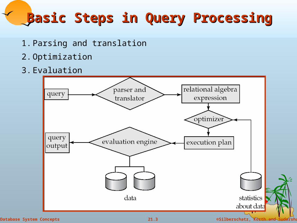
1. Parsing and translation

2. Optimization

3. Evaluation

4


Basic Steps in Query Processing Basic Steps in Query Processing (Cont.)(Cont.)

Parsing and translation translate the query into its internal form. This is then translated into

relational algebra. Parser checks syntax, verifies relations

Evaluation The query-execution engine takes a query-evaluation plan, executes

that plan, and returns the answers to the query. Query Optimization: Amongst all equivalent evaluation plans

choose the one with lowest cost. Cost is estimated using statistical information from the

database catalog e.g. number of tuples in each relation, size of tuples, etc.

5


Basic Steps in Query Processing : Basic Steps in Query Processing : OptimizationOptimization

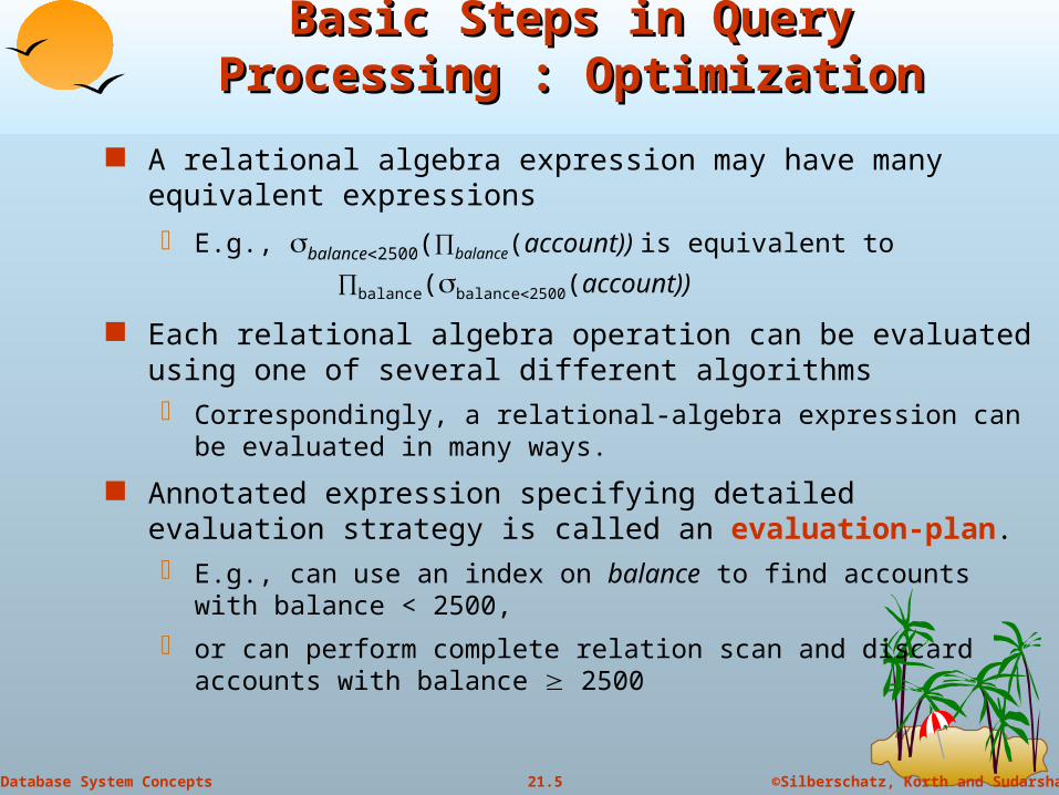
A relational algebra expression may have many equivalent expressions E.g., balance2500(balance(account)) is equivalent to

balance(balance2500(account))

Each relational algebra operation can be evaluated using one of several different algorithms Correspondingly, a relational-algebra expression can be evaluated in

many ways. Annotated expression specifying detailed evaluation strategy is

called an evaluation-plan. E.g., can use an index on balance to find accounts with balance < 2500, or can perform complete relation scan and discard accounts with

balance 2500

6


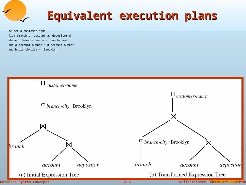
Equivalent execution plansEquivalent execution plansselect d.customer-name

from branch b, account a, depositor d

where b.branch-name = a.branch-name

and a.account-number = d.account-number

and b.branch-city = ‘Brooklyn’

7


Measures of Query CostMeasures of Query Cost Cost is generally measured as total elapsed time for

answering query Many factors contribute to time cost

disk accesses, CPU, or even network communication Typically disk access is the predominant cost, and is also

relatively easy to estimate. Measured by taking into account Number of seeks * average-seek-cost Number of blocks read * average-block-read-cost Number of blocks written * average-block-write-cost

Cost to write a block is greater than cost to read a block – data is read back after being written to ensure that the

write was successful ( MAIS o CUSTO DAS TRANSACÇÔES!!!)

8


SORTINGSORTING

9


SortingSorting We may build an index on the relation, and then use the index to

read the relation in sorted order. May lead to one disk block access for each tuple.

For relations that fit in memory, techniques like quicksort can be used. For relations that don’t fit in memory, external sort-merge is a good choice.

10


External Sort-MergeExternal Sort-Merge

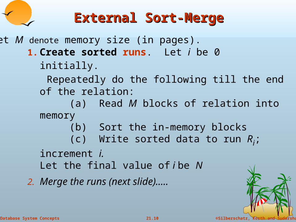
1. Create sorted runs. Let i be 0 initially. Repeatedly do the following till the end of the relation: (a) Read M blocks of relation into memory (b) Sort the in-memory blocks (c) Write sorted data to run Ri; increment i.Let the final value of i be N

2. Merge the runs (next slide)…..

Let M denote memory size (in pages).

11


External Sort-Merge (Cont.)External Sort-Merge (Cont.)

2. Merge the runs (N-way merge). We assume (for now) that N < M. 1. Use N blocks of memory to buffer input runs, and 1 block to

buffer output. Read the first block of each run into its buffer page

2. repeat1. Select the first record (in sort order) among all buffer pages

2. Write the record to the output buffer. If the output buffer is full write it to disk.

3. Delete the record from its input buffer page.If the buffer page becomes empty then read the next block (if any) of the run into the buffer.

3. until all input buffer pages are empty:

12


External Sort-Merge (Cont.)External Sort-Merge (Cont.)

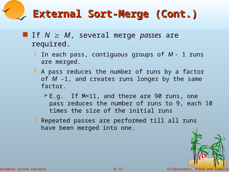
If N M, several merge passes are required. In each pass, contiguous groups of M - 1 runs are merged. A pass reduces the number of runs by a factor of M -1, and

creates runs longer by the same factor. E.g. If M=11, and there are 90 runs, one pass reduces

the number of runs to 9, each 10 times the size of the initial runs

Repeated passes are performed till all runs have been merged into one.

13


Example: External Sorting Using Sort-MergeExample: External Sorting Using Sort-Merge

14


JOINJOIN

15


Nested-Loop (NL) JoinNested-Loop (NL) Join

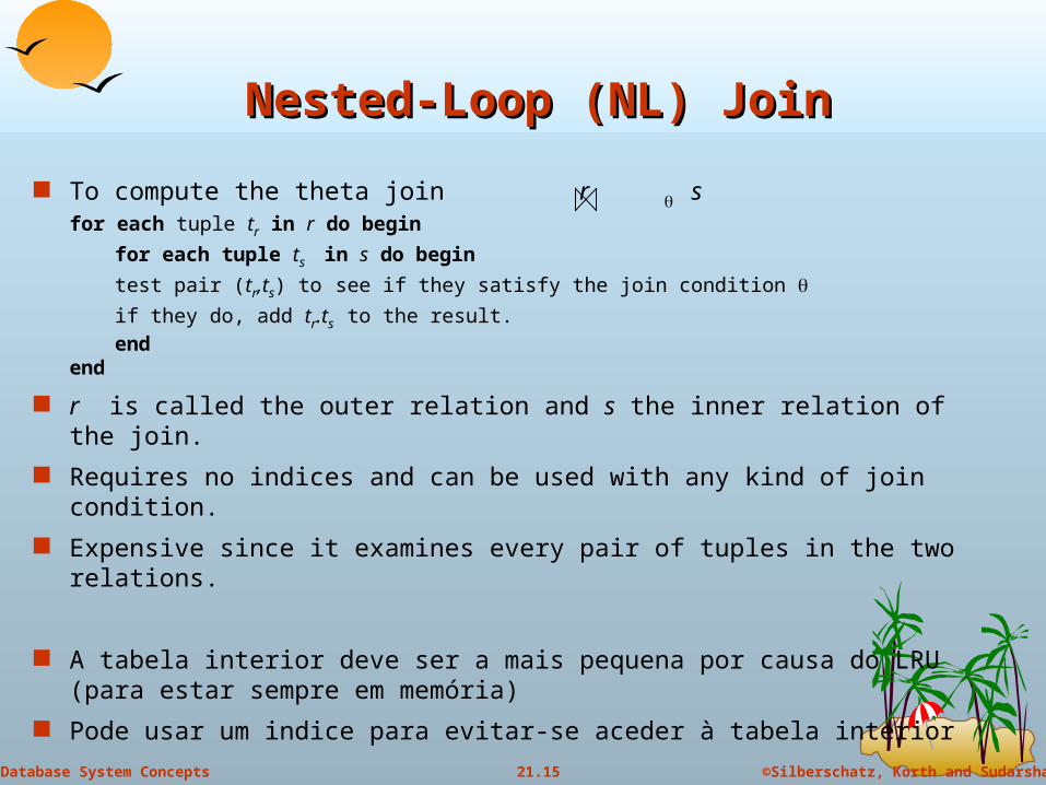
To compute the theta join r sfor each tuple tr in r do begin

for each tuple ts in s do begintest pair (tr,ts) to see if they satisfy the join condition if they do, add tr.ts to the result.

endend

r is called the outer relation and s the inner relation of the join. Requires no indices and can be used with any kind of join condition. Expensive since it examines every pair of tuples in the two relations.

A tabela interior deve ser a mais pequena por causa do LRU (para estar sempre em memória)

Pode usar um indice para evitar-se aceder à tabela interior

16


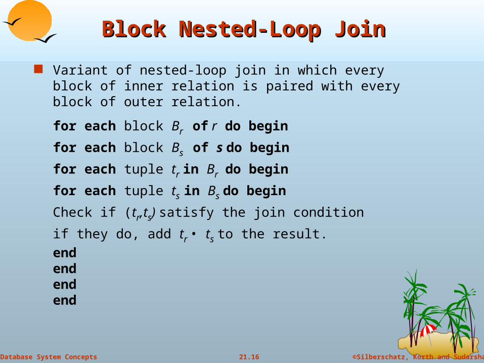
Block Nested-Loop JoinBlock Nested-Loop Join Variant of nested-loop join in which every block of inner

relation is paired with every block of outer relation.

for each block Br of r do beginfor each block Bs of s do begin

for each tuple tr in Br do beginfor each tuple ts in Bs do begin

Check if (tr,ts) satisfy the join condition

if they do, add tr • ts to the result.end

endend

end

17


Merge-JoinMerge-Join

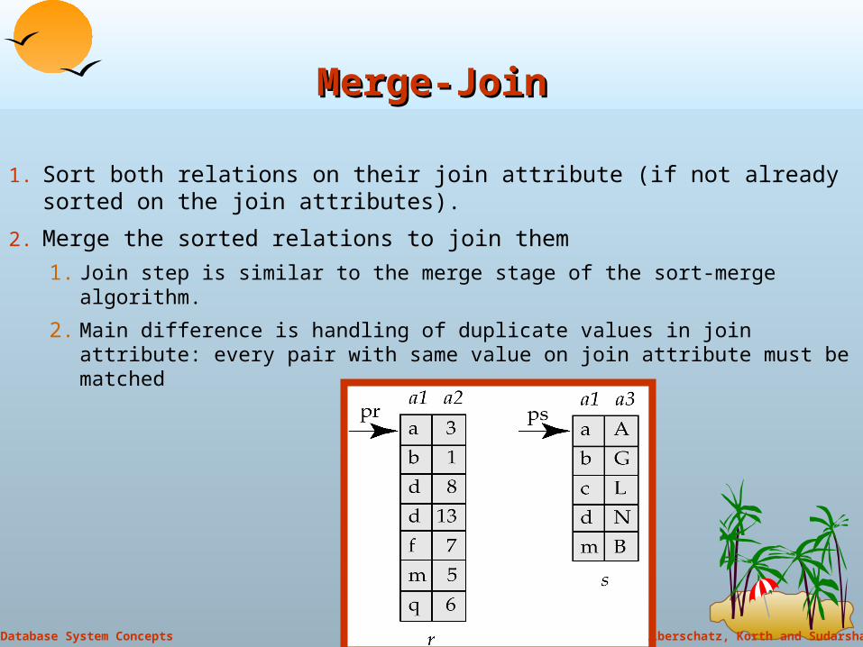
1. Sort both relations on their join attribute (if not already sorted on the join attributes).

2. Merge the sorted relations to join them1. Join step is similar to the merge stage of the sort-merge algorithm.

2. Main difference is handling of duplicate values in join attribute: every pair with same value on join attribute must be matched

18


Hash-Join AlgorithmHash-Join Algorithm

1. Partition the relation s using hashing function h. When partitioning a relation, one block of memory is reserved as the output buffer for each partition.

2. Partition r similarly.

3. For each i:(a)Load si into memory and build an in-memory hash index on it

using the join attribute. This hash index uses a different hash function than the earlier one h.

(b)Read the tuples in ri from the disk one by one. For each tuple tr locate each matching tuple ts in si using the in-memory hash index. Output the concatenation of their attributes.

The hash-join of r and s is computed as follows.

Relation s is called the build input and r is called the probe input.

19


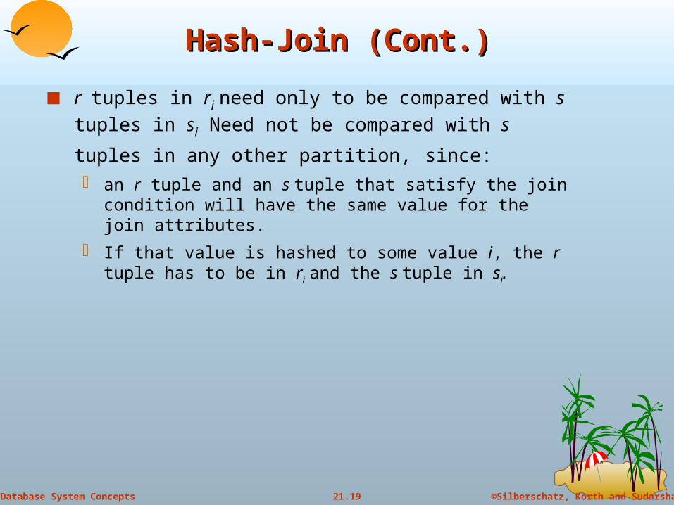
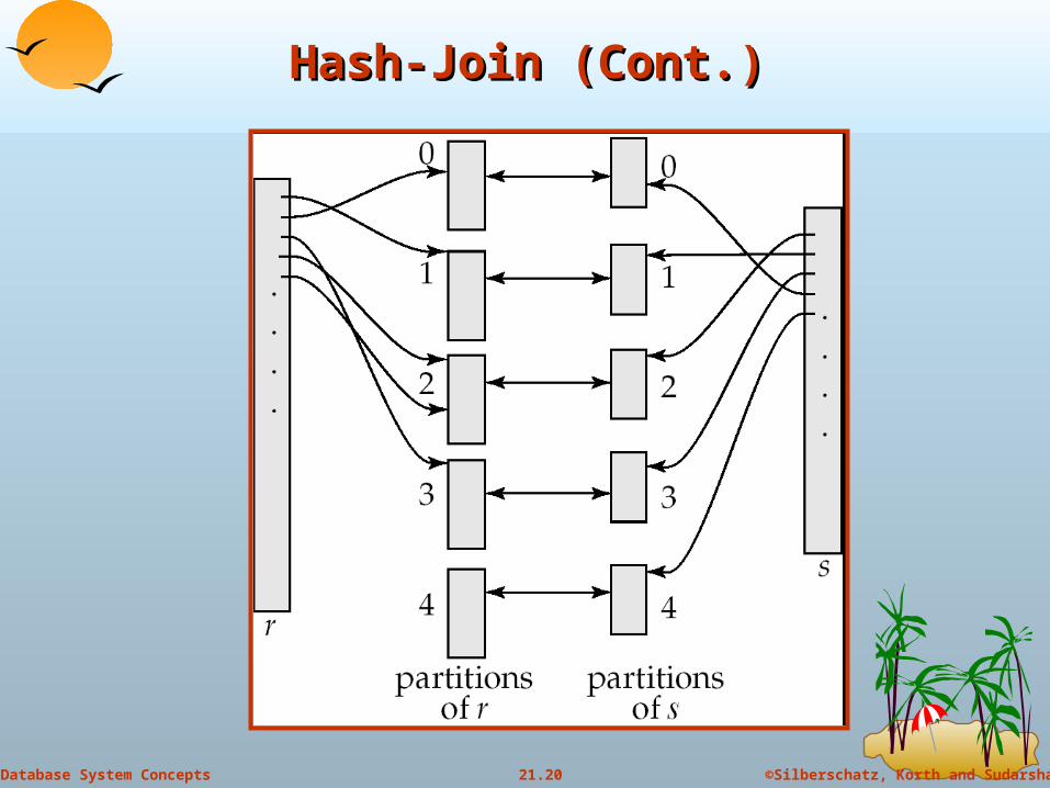
Hash-Join (Cont.)Hash-Join (Cont.)

r tuples in ri need only to be compared with s tuples in si

Need not be compared with s tuples in any other partition, since: an r tuple and an s tuple that satisfy the join condition will have

the same value for the join attributes. If that value is hashed to some value i, the r tuple has to be in ri

and the s tuple in si.

20


Hash-Join (Cont.)Hash-Join (Cont.)

21


Índices - revisãoÍndices - revisão O que é:

É uma estrutura auxiliar de acesso à informação Um índice definido sobre uma chave K, permite aceder

rapidamente aos registos contendo a chave K. Um índice tem 2 componentes:

A que permite encontrar a chave K dentro do índice A que permite encontar a informação dos registos que contêm a

chave K A chave pode ser composta por vários atributos Podem existir vários índices sobre a mesma tabela/atributos A alteração/remoção/inserção do valor de K de algum registo na

tabela implica a re-ordenação da estrutura de índice.

22


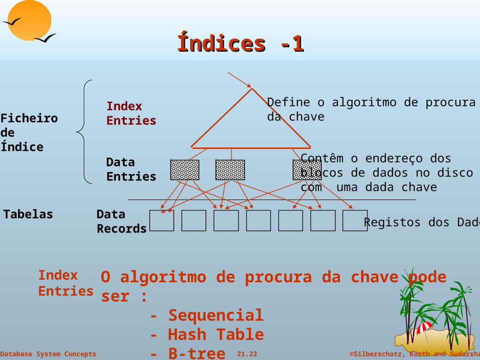
Índices -1Índices -1

Data Records

IndexEntries

Registos dos Dados

Ficheiro de Índice

Define o algoritmo de procura da chave

DataEntries

Contêm o endereço dos blocos de dados no disco com uma dada chave

Tabelas

IndexEntries

O algoritmo de procura da chave pode ser :- Sequencial- Hash Table- B-tree

23


Índices - 2Índices - 2

Data Records Registos dos Dados

Ficheiro de Índice


DataEntries Contêm o endereço dos blocos

de dados no disco

Tabelas

Data Entries

Contêm 1 de 3 hipóteses:- O próprio Data record com chave k- <k, endereço do data record no disco com chave

k>- <k, lista de endereços de data records no disco

com chave k>

IndexEntries

24




Ficheiro de Índice



de dados no disco

Tabelas

Data Records

- Contêm os dados propriamente ditos- Podem:

- não estar ordenados fisicamente pela chave k (tal como figura em cima)- estar ordenados fisicamente pela

chave k (tal como figura do próximo slide)

IndexEntries

25




Ficheiro de Índice



de dados no disco

Tabelas

Data Records

- Quando os registos estão ordenados fisicamente, diz-se que a tabela/indíce está “Clustered”

IndexEntries

26


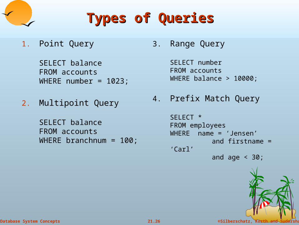
Types of QueriesTypes of Queries

1. Point Query

SELECT balanceFROM accountsWHERE number = 1023;

2. Multipoint Query

SELECT balanceFROM accountsWHERE branchnum = 100;

3. Range Query

SELECT numberFROM accountsWHERE balance > 10000;

4. Prefix Match Query

SELECT *FROM employeesWHERE name = ‘Jensen’

and firstname = ‘Carl’ and age < 30;

27


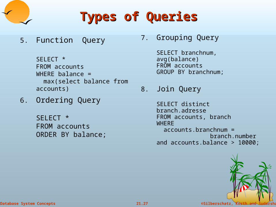
Types of QueriesTypes of Queries

5. Function Query

SELECT *FROM accountsWHERE balance = max(select balance from accounts)

6. Ordering Query

SELECT *FROM accountsORDER BY balance;

7. Grouping Query

SELECT branchnum, avg(balance)FROM accountsGROUP BY branchnum;

8. Join Query

SELECT distinct branch.adresseFROM accounts, branchWHERE accounts.branchnum =

branch.numberand accounts.balance > 10000;

28


Heurísticas de criação de índices (1)Heurísticas de criação de índices (1)

Quando as queries forem simples. Se não os índices não são usados!!!! Exemplo, se um atributo

aparece como argumento de uma função os índices não são normalmente usados.

Quando os resultados representarem uma pequena proporção do total da tabela (< 20%) ?

Quando os valores distintos de uma coluna representarem uma pequena proporção do total dos valores da coluna (<5%) ?

Se houver condições com multiplos atributos: As chaves compostas devem que ser declaradas da mesma ordem

que usadas As chaves compostas podem ser usadas para incluir no Data

Entries a própria resposta à query..

29


Heurísticas de criação de índices (2)Heurísticas de criação de índices (2)

Quando a chave for usada em condições nas Cláusulas de Where. Condições de “range” sugerem índices sequenciais ou Btree Condições de igualdade sugerem índices hashed

Quando a tabela for grande (o número de Data Records for grande)

Só se não existirem muitos outros índices na mesma tabela

30


Heurísticas de criação de índices(3)Heurísticas de criação de índices(3) Como um índice sobre a chave K:

acelera as leituras de registos identificados por k acelera os updates de atributos (que não sejam parte de K) e que

sejam de registos identificados por k atrasa as inserções e eliminações de registos atrasa as alterações aos atributos que pertencem à chave K

Só será interessante quando o número acessos dos dois primeiros cenários for bastante superior ao número de acessos dos dois últimos cenários.

Regra por omissão é 1 para 5!!

31


Heurísticas para a criação de Ìndices Heurísticas para a criação de Ìndices “Clustered”“Clustered”

Os índices Clustered implicam a re-ordenação física dos dados sempre que são

inseridos novos registos na tabela. Optimizam as pesquisas de “ranges” (intervalos)

Logo só são interessantes quando: existem queires importantes com cláusulas de Where com “ranges” as insersões/modificações da chave são pouco frequentes (ou

então se o factor de compactação for muito baixo.)

32


Heurísticas para a criação de Ìndices Heurísticas para a criação de Ìndices “Bitmaps”“Bitmaps”

Os índices bitmaps implicam a criação de um array de bits por cada valor discreto que

a coluna assume Logo só são interessantes quando:

Os valores distintos de uma coluna são uma pequena % dos valores totais da coluna (< 0,1%)

as insersões/modificações da são reduzidas

33


Agregração de várias tabelasAgregração de várias tabelas É possível definir um Índice Clustered de várias

tabelas simultâneamente. Exemplo 1:

Pessoa(BI, Nome, Morada), Carro(Mat, marca, BI),

Um Índice em BI clustered sobre Pessoa e Carro seria armazenado da seguinte forma:

BI=100 Joao, Lisboa Bx-23-45, Fiat 00-23-IP, Rover

BI=110 Pedro, Sintra XX-23-45, Fiat 00-23-II, Opel 33-23-II, Opel 00-23-II, Opel

BI=200 Pedro, Sintra

BI=201 Rui, Almada

100, Joao, Lisboa

110, Pedro, Sintra

200, Pedro, Sintra

201, Rui, Almada

Bx-23-45, Fiat, 100

00-23-IP, Rover, 100

XX-23-45, Fiat, 110

00-23-II, Opel, 110

33-23-II, Opel, 110

00-23-II, Opel, 110


Indexes with Composite Search Keys Indexes with Composite Search Keys Composite Search Keys: Search on a

combination of fields. Equality query: Every field value is equal

to a constant value. E.g. wrt <sal,age> index: age=20 and sal =75

Range query: Some field value is not a constant. E.g.: age =20; or age=20 and sal > 10

Data entries in index sorted by search key to support range queries. Lexicographic order, or Spatial order.

sue 13 75

bobcaljoe 12

10

208011

12

name age sal

<sal, age>

<age, sal> <age>

<sal>

12,2012,10

11,80

13,75

20,12

10,12

75,1380,11

11121213

10207580

Data recordssorted by name

Data entries in indexsorted by <sal,age>

Data entriessorted by <sal>

Examples of composite keyindexes using lexicographic order.

35


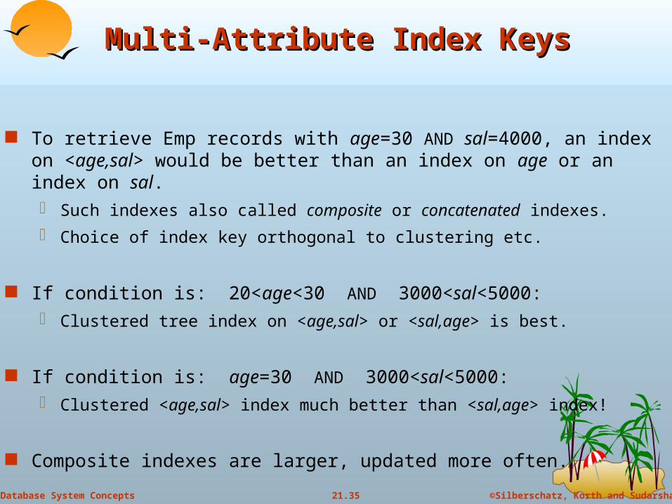
Multi-Attribute Index KeysMulti-Attribute Index Keys

To retrieve Emp records with age=30 AND sal=4000, an index on <age,sal> would be better than an index on age or an index on sal. Such indexes also called composite or concatenated indexes. Choice of index key orthogonal to clustering etc.

If condition is: 20<age<30 AND 3000<sal<5000: Clustered tree index on <age,sal> or <sal,age> is best.

If condition is: age=30 AND 3000<sal<5000: Clustered <age,sal> index much better than <sal,age> index!

Composite indexes are larger, updated more often.

36


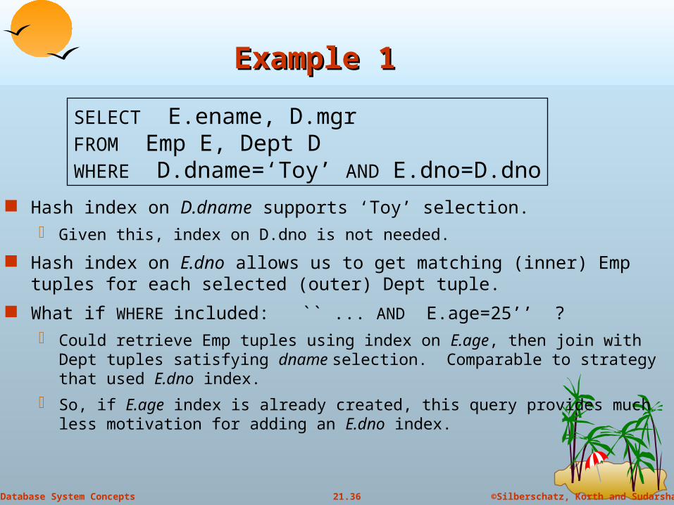
Example 1Example 1

Hash index on D.dname supports ‘Toy’ selection. Given this, index on D.dno is not needed.

Hash index on E.dno allows us to get matching (inner) Emp tuples for each selected (outer) Dept tuple.

What if WHERE included: `` ... AND E.age=25’’ ? Could retrieve Emp tuples using index on E.age, then join with Dept tuples

satisfying dname selection. Comparable to strategy that used E.dno index. So, if E.age index is already created, this query provides much less motivation

for adding an E.dno index.

SELECT E.ename, D.mgrFROM Emp E, Dept DWHERE D.dname=‘Toy’ AND E.dno=D.dno

37


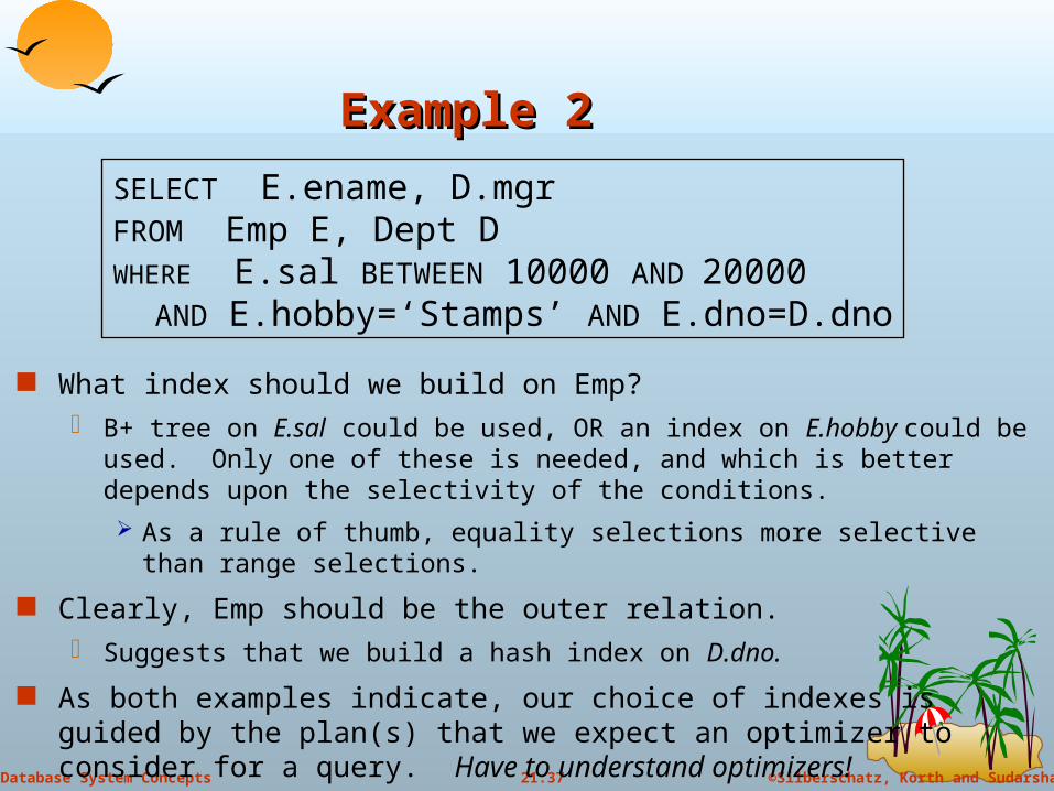
Example 2Example 2

What index should we build on Emp? B+ tree on E.sal could be used, OR an index on E.hobby could be used. Only

one of these is needed, and which is better depends upon the selectivity of the conditions. As a rule of thumb, equality selections more selective than range selections.

Clearly, Emp should be the outer relation. Suggests that we build a hash index on D.dno.

As both examples indicate, our choice of indexes is guided by the plan(s) that we expect an optimizer to consider for a query. Have to understand optimizers!

SELECT E.ename, D.mgrFROM Emp E, Dept DWHERE E.sal BETWEEN 10000 AND 20000 AND E.hobby=‘Stamps’ AND E.dno=D.dno

38


Examples of ClusteringExamples of Clustering

B+ tree index on E.age can be used to get qualifying tuples. How selective is the condition? Is the index clustered?

Consider the GROUP BY query. If many tuples have E.age > 10, using E.age

index and sorting the retrieved tuples may be costly.

Clustered E.dno index may be better!

Equality queries and duplicates: Clustering on E.hobby helps!

SELECT E.dnoFROM Emp EWHERE E.age>40

SELECT E.dno, COUNT (*)FROM Emp EWHERE E.age>10GROUP BY E.dno

SELECT E.dnoFROM Emp EWHERE E.hobby=´Stamps´

39


Clustering and JoinsClustering and Joins

Clustering is especially important when accessing inner tuples. Should make index on E.dno clustered.

Suppose that the WHERE clause is instead:WHERE E.hobby=‘Stamps´ AND E.dno=D.dno If many employees collect stamps, Sort-Merge join may be worth considering. A

clustered index on D.dno would help. Summary: Clustering is useful whenever many tuples are to be retrieved.

SELECT E.ename, D.mgrFROM Emp E, Dept DWHERE D.dname=‘Toy’ AND E.dno=D.dno

40


Index-Only PlansIndex-Only Plans

A number of queries can be answered without retrieving any tuples from one or more of the relations involved if a suitable index is available.

SELECT D.mgrFROM Dept D, Emp EWHERE D.dno=E.dnoSELECT D.mgr, E.eidFROM Dept D, Emp EWHERE D.dno=E.dno

SELECT E.dno, COUNT(*)FROM Emp EGROUP BY E.dno

SELECT E.dno, MIN(E.sal)FROM Emp EGROUP BY E.dno

SELECT AVG(E.sal)FROM Emp EWHERE E.age=25 AND E.sal BETWEEN 3000 AND 5000

<E.dno><E.dno,E.eid>

Tree index!

<E.dno>

<E.dno,E.sal>Tree index!

<E. age,E.sal> or<E.sal, E.age>

Tree!

Documents

©Silberschatz, Korth and SudarshanDatabase System Concepts 21.1 Chapter 13: Query Processing