Similarity Ranking in Large-Scale Bipartite Graphs

Brown University - 20th March 2014!1

Alessandro Epasto

!2

Joint work with J. Feldman, S. Lattanzi, S. Leonardi, V. Mirrokni [WWW, 2014]

AdWords

Ads

Ads

Our Goal

●Tackling AdWords data to identify automatically, for each advertiser, its main competitors and suggest relevant queries to each advertiser. !●Goals: ● Useful business information. ● Improve advertisement. ●More relevant performance benchmarks.

The Data

Large advertisers (e.g., Amazon, Ask.com, etc) compete in several market segments with very different advertisers.

Query Information

Nike store New York Market Segment: Retailer, Geo: NY (USA), Stats: 10 clicks

Soccer shoes Market Segment: Apparel, Geo: London, UK, Stats: 4 clicks

Soccer ball Market Segment: Equipment Geo: San Francisco (USA), Stats: 5 clicks

…. millions of other queries ….

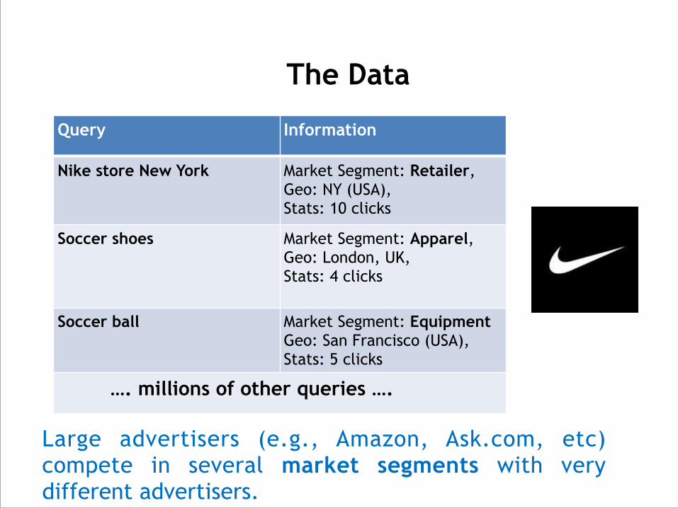
Modeling the Data as a Bipartite Graph

Millions of Advertisers Billions of Queries

Hundreds of Labels

Other Applications

● General approach applicable to several contexts: ●User, Movies, Categories: find similar

users and suggest movies. ● Authors, Papers, Conferences: find

related authors and suggest papers to read.

!● Generally this bipartite graphs are lopsided:

we want algorithms with complexity depending on the smaller side.

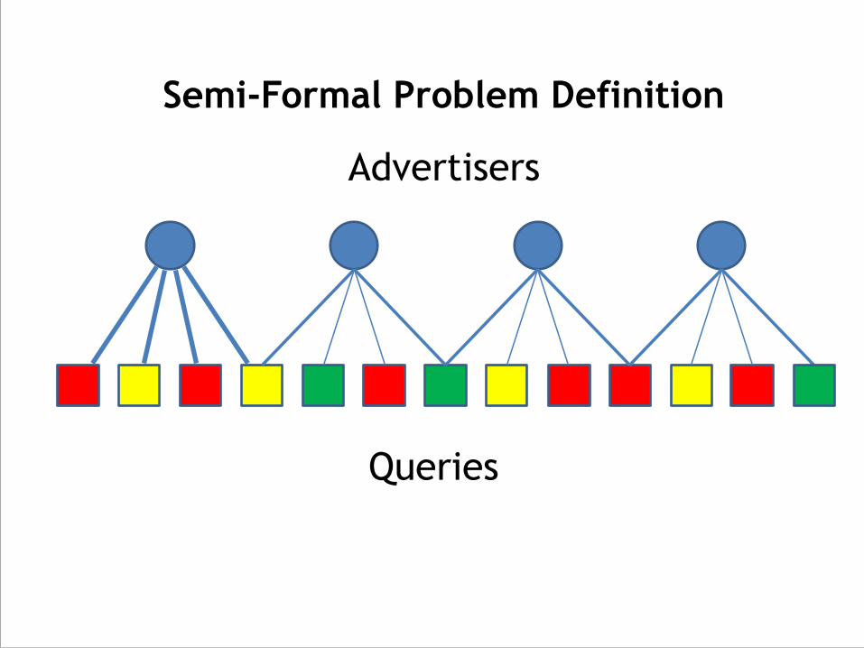
Semi-Formal Problem Definition

Advertisers

Queries

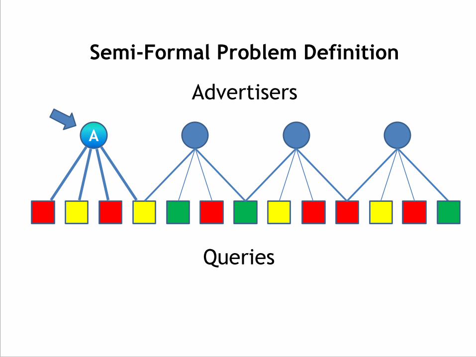
Semi-Formal Problem Definition

A

Advertisers

Queries

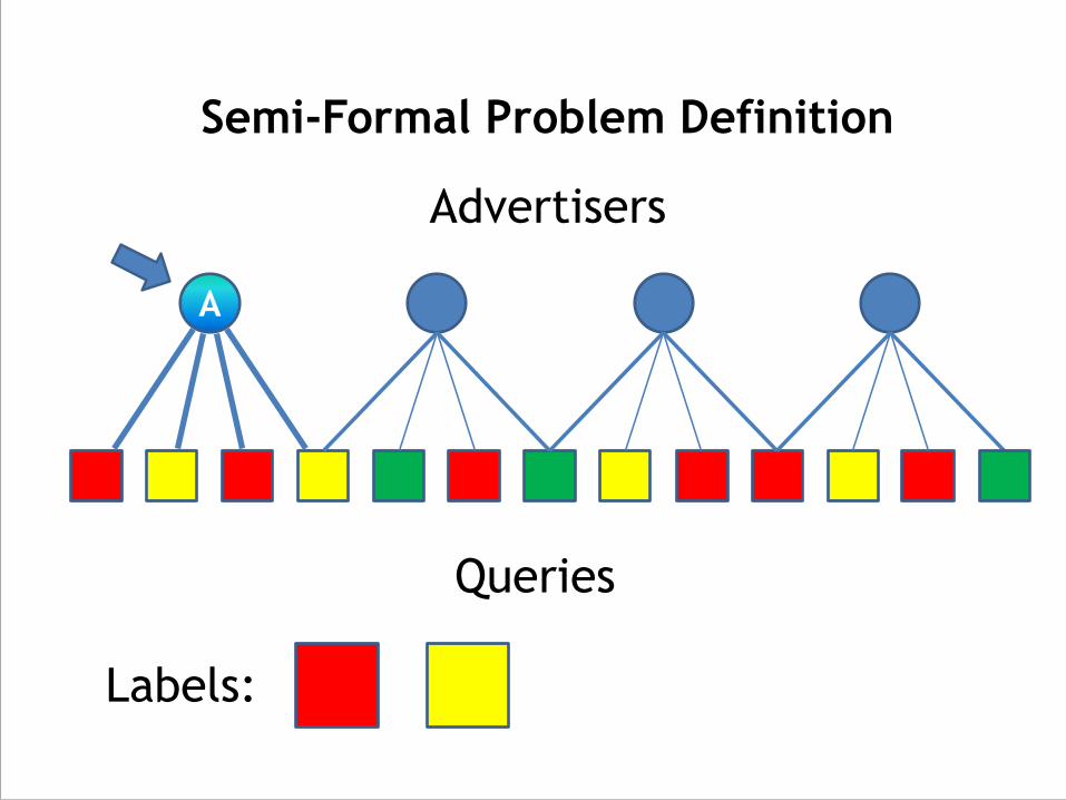
Semi-Formal Problem Definition

A

Advertisers

Queries

Labels:

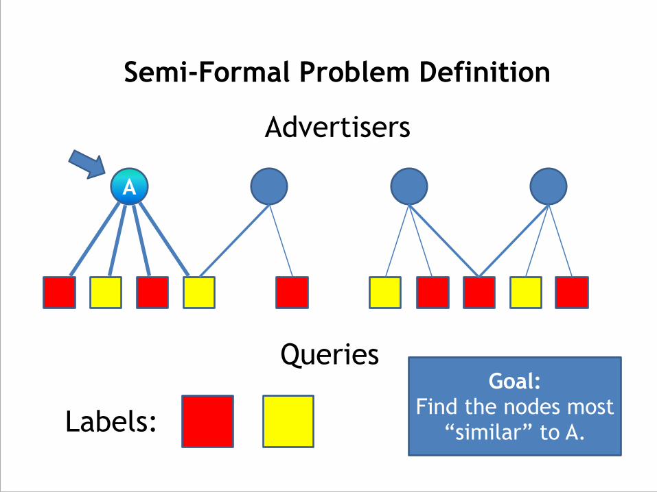
Semi-Formal Problem Definition

A

Advertisers

Queries

Labels:Goal:

Find the nodes most “similar” to A.

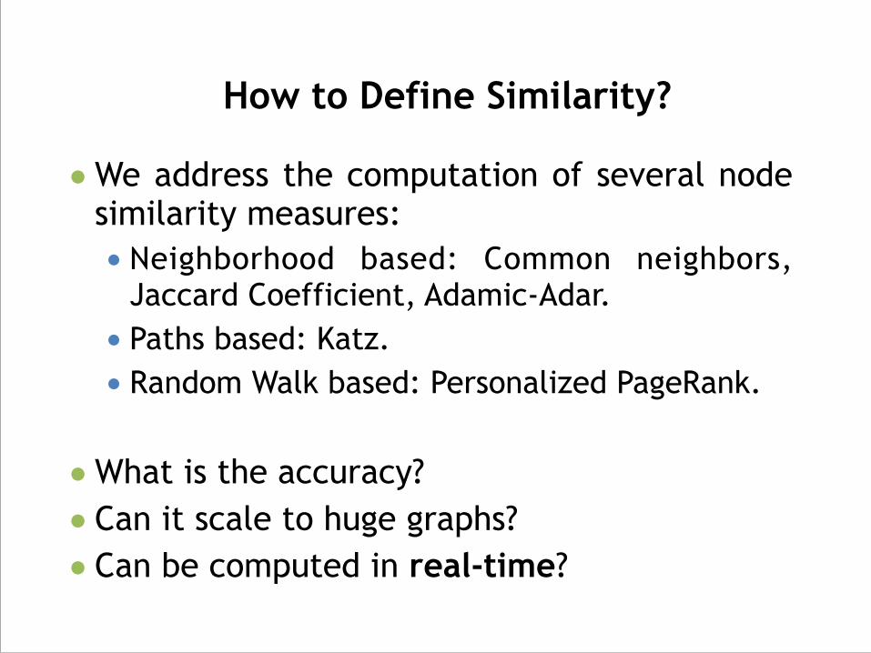
How to Define Similarity?

●We address the computation of several node similarity measures: ● Neighborhood based: Common neighbors,

Jaccard Coefficient, Adamic-Adar. ● Paths based: Katz. ● Random Walk based: Personalized PageRank.

!●What is the accuracy? ● Can it scale to huge graphs? ● Can be computed in real-time?

Our Contribution

● Reduce and Aggregate: general approach to induce real-time similarity rankings in multi-categorical bipartite graphs, that we apply to several similarity measures. !

● Theoretical guarantees for the precision of the algorithms. !

● Experimental evaluation with real world data.

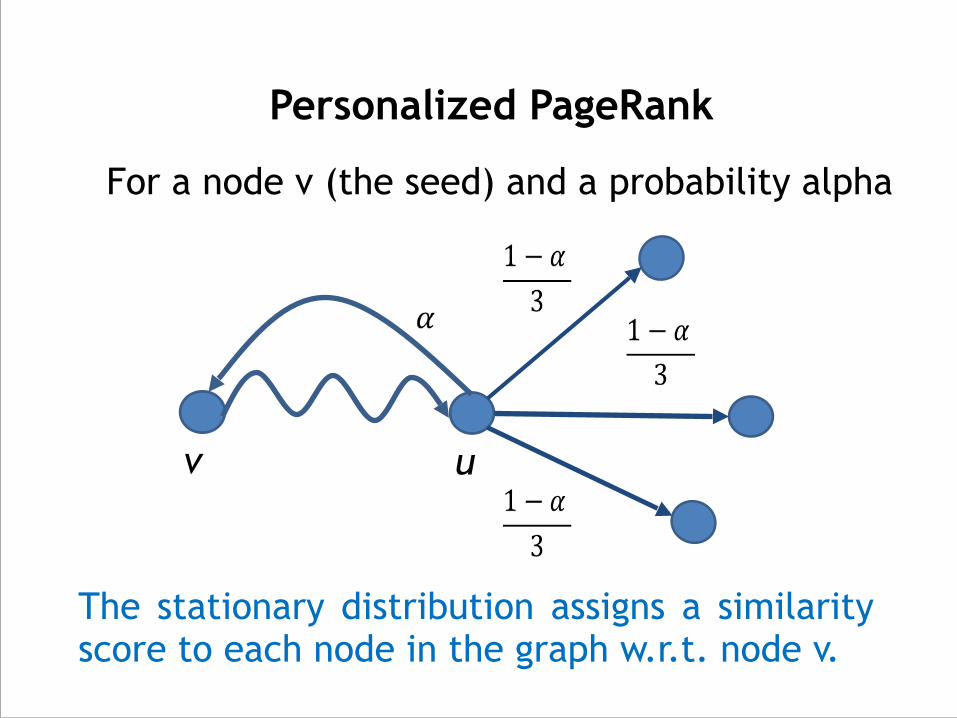
Personalized PageRank

v u

 

 

 

 

The stationary distribution assigns a similarity score to each node in the graph w.r.t. node v. !!

For a node v (the seed) and a probability alpha

Personalized PageRank

● Extensive algorithmic literature. !

● Very good accuracy in our experimental evaluation compared to other similarities (Jaccard, Intersection, etc.). !

● Efficient MapReduce algorithm scaling to large graphs (hundred of millions of nodes).

However…

Personalized PageRank

!!!

!!● Our graphs are too big (billions of nodes) even for

large-scale systems. ● MapReduce is not real-time. ● We cannot pre-compute the rankings for each

subset of labels.

Reduce and Aggregate

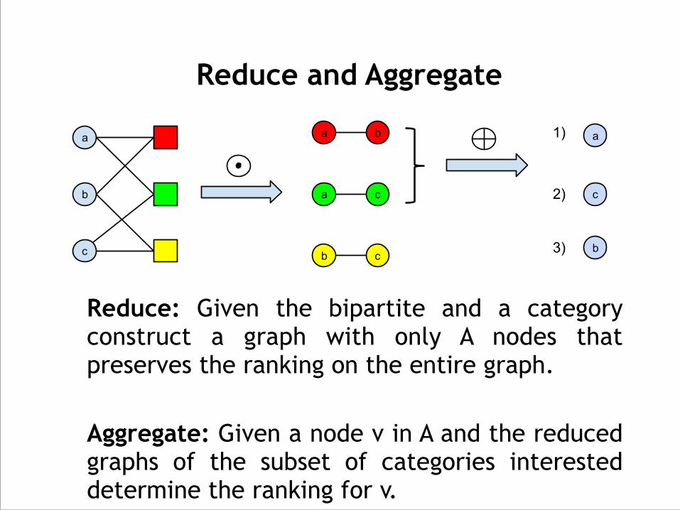
Reduce: Given the bipartite and a category construct a graph with only A nodes that preserves the ranking on the entire graph. !Aggregate: Given a node v in A and the reduced graphs of the subset of categories interested determine the ranking for v.

D

E

F

D E

F

F

D

E

D

F

��

E

��

��

In practice

!!!!

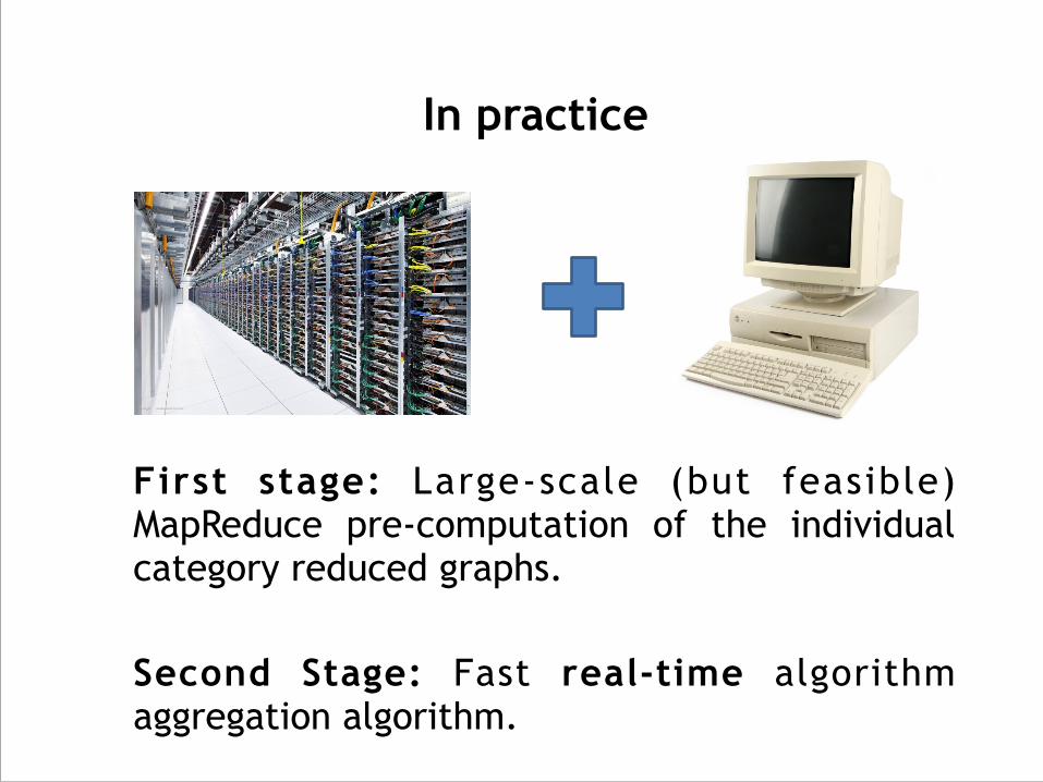
!First stage: Large-scale (but feasible) MapReduce pre-computation of the individual category reduced graphs. !Second Stage: Fast real-time algorithm aggregation algorithm.

Reduce for Personalized PageRank

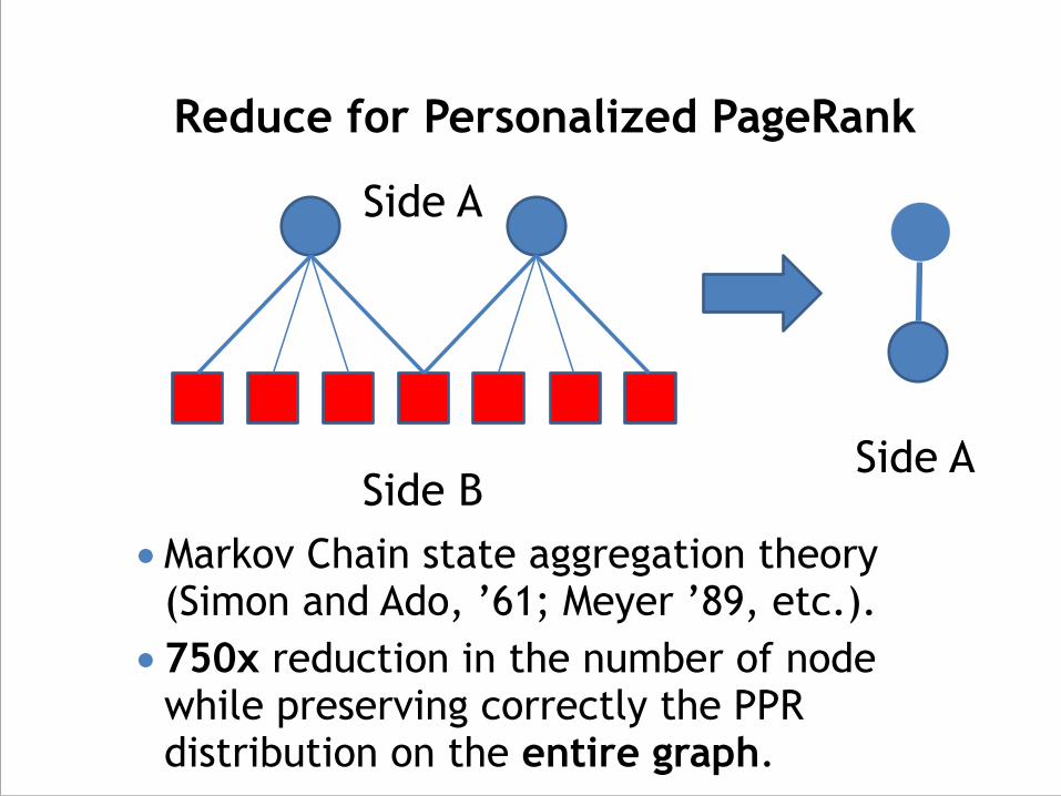
●Markov Chain state aggregation theory (Simon and Ado, ’61; Meyer ’89, etc.).

● 750x reduction in the number of node while preserving correctly the PPR distribution on the entire graph.

Side A

Side BSide A

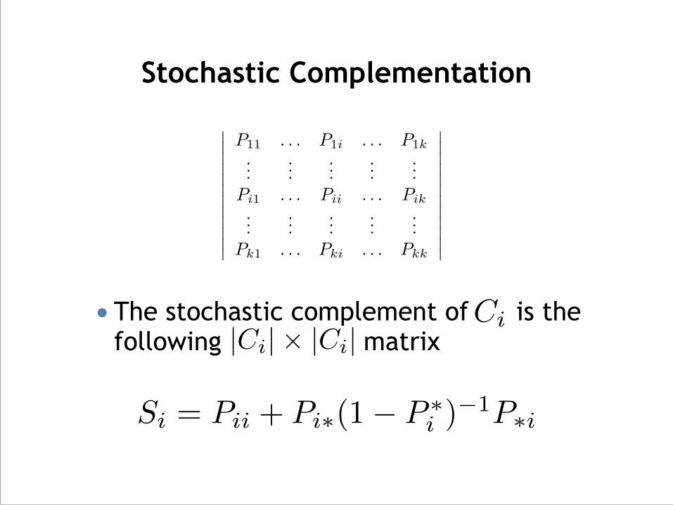
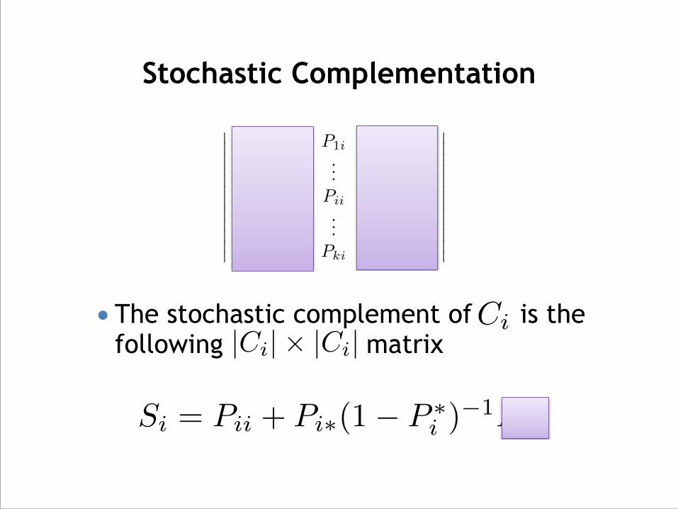
Stochastic Complementation

● The stochastic complement of is the following matrix

Ci

Si = Pii + Pi⇤(1� P ⇤i )

�1P⇤i

|Ci|⇥ |Ci|

������������

P11 . . . P1i . . . P1k...

......

......

Pi1 . . . Pii . . . Pik...

......

......

Pk1 . . . Pki . . . Pkk

������������

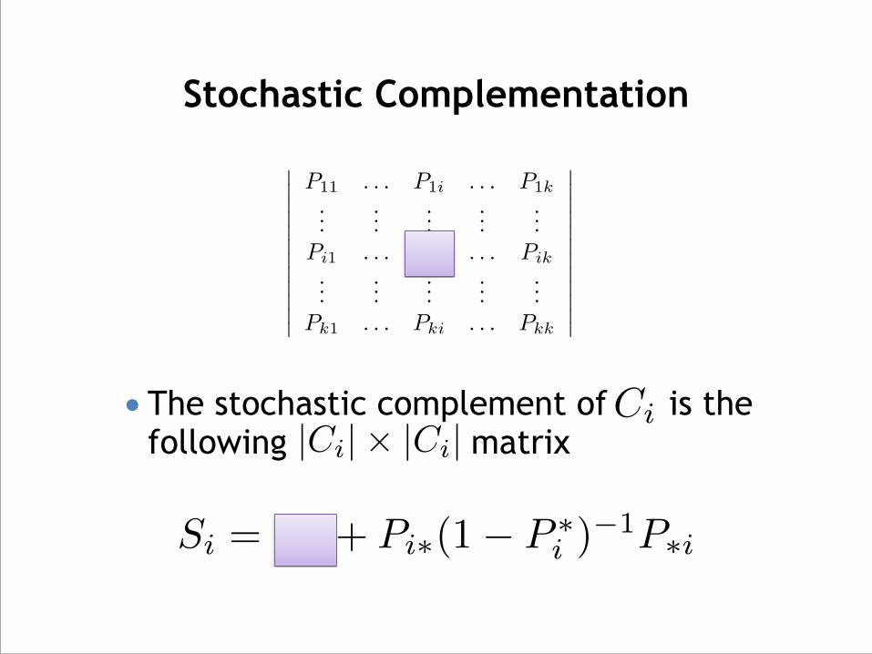
Stochastic Complementation

● The stochastic complement of is the following matrix

Ci

Si = Pii + Pi⇤(1� P ⇤i )

�1P⇤i

|Ci|⇥ |Ci|

������������

P11 . . . P1i . . . P1k...

......

......

Pi1 . . . Pii . . . Pik...

......

......

Pk1 . . . Pki . . . Pkk

������������

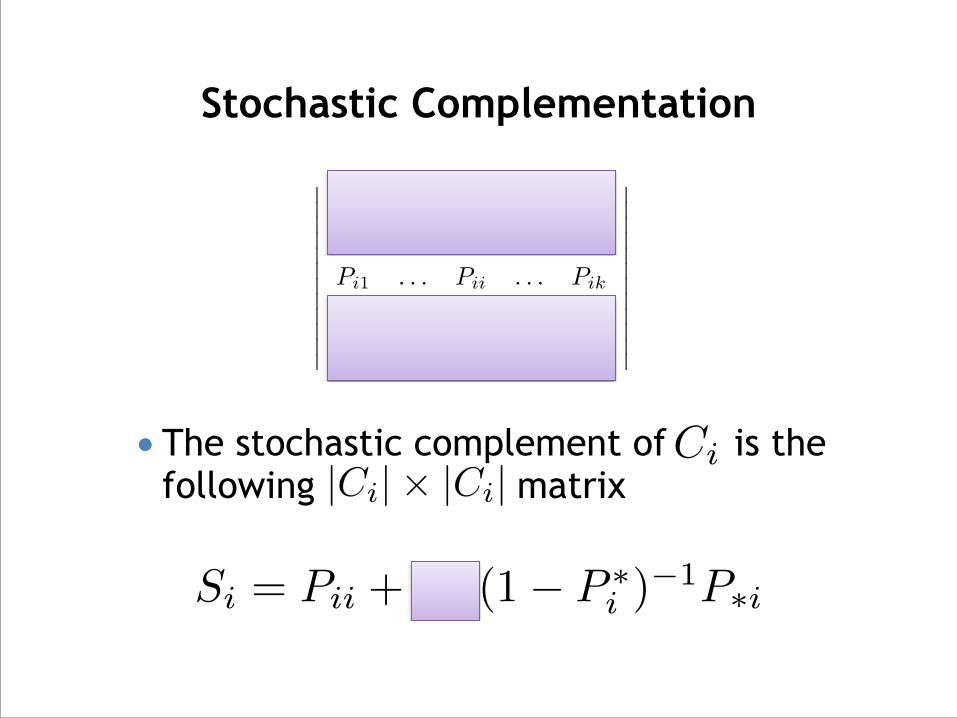
Stochastic Complementation

● The stochastic complement of is the following matrix

Ci

Si = Pii + Pi⇤(1� P ⇤i )

�1P⇤i

|Ci|⇥ |Ci|

������������

P11 . . . P1i . . . P1k...

......

......

Pi1 . . . Pii . . . Pik...

......

......

Pk1 . . . Pki . . . Pkk

������������

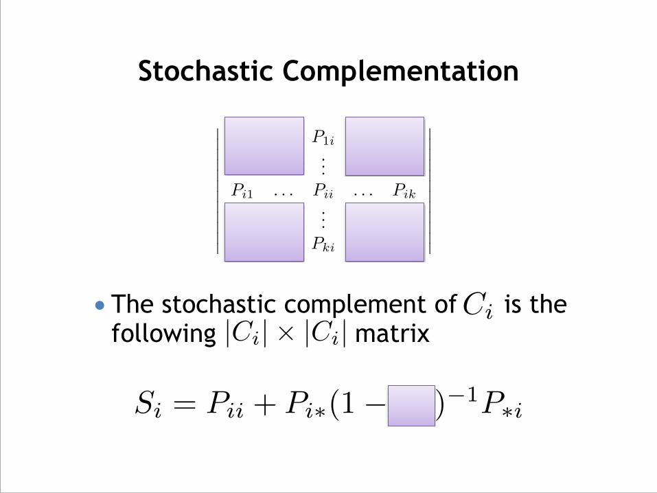
Stochastic Complementation

● The stochastic complement of is the following matrix

Ci

Si = Pii + Pi⇤(1� P ⇤i )

�1P⇤i

|Ci|⇥ |Ci|

������������

P11 . . . P1i . . . P1k...

......

......

Pi1 . . . Pii . . . Pik...

......

......

Pk1 . . . Pki . . . Pkk

������������

Stochastic Complementation

● The stochastic complement of is the following matrix

Ci

Si = Pii + Pi⇤(1� P ⇤i )

�1P⇤i

|Ci|⇥ |Ci|

������������

P11 . . . P1i . . . P1k...

......

......

Pi1 . . . Pii . . . Pik...

......

......

Pk1 . . . Pki . . . Pkk

������������

Stochastic Complementation

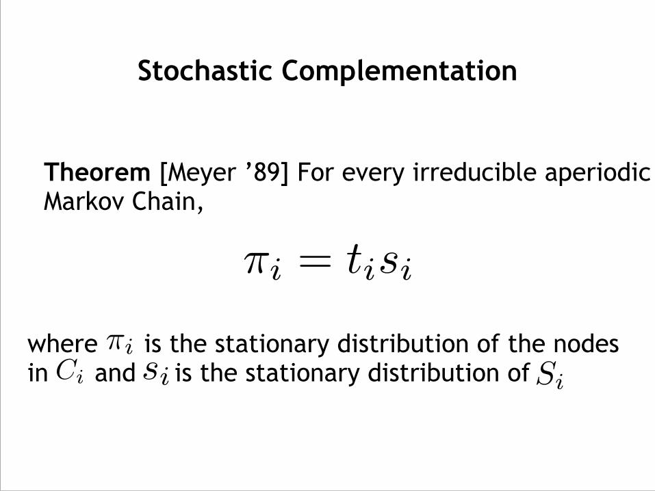
⇡i = tisi

Theorem [Meyer ’89] For every irreducible aperiodic Markov Chain,

where is the stationary distribution of the nodes in and is the stationary distribution of

⇡iCi si Si

Stochastic Complementation

● Computing the stochastic complements is unfeasible in general for large matrices (matrix inversion).

!● In our case we can exploit the properties

of random walks on Bipartite graphs to invert the matrix analytically.

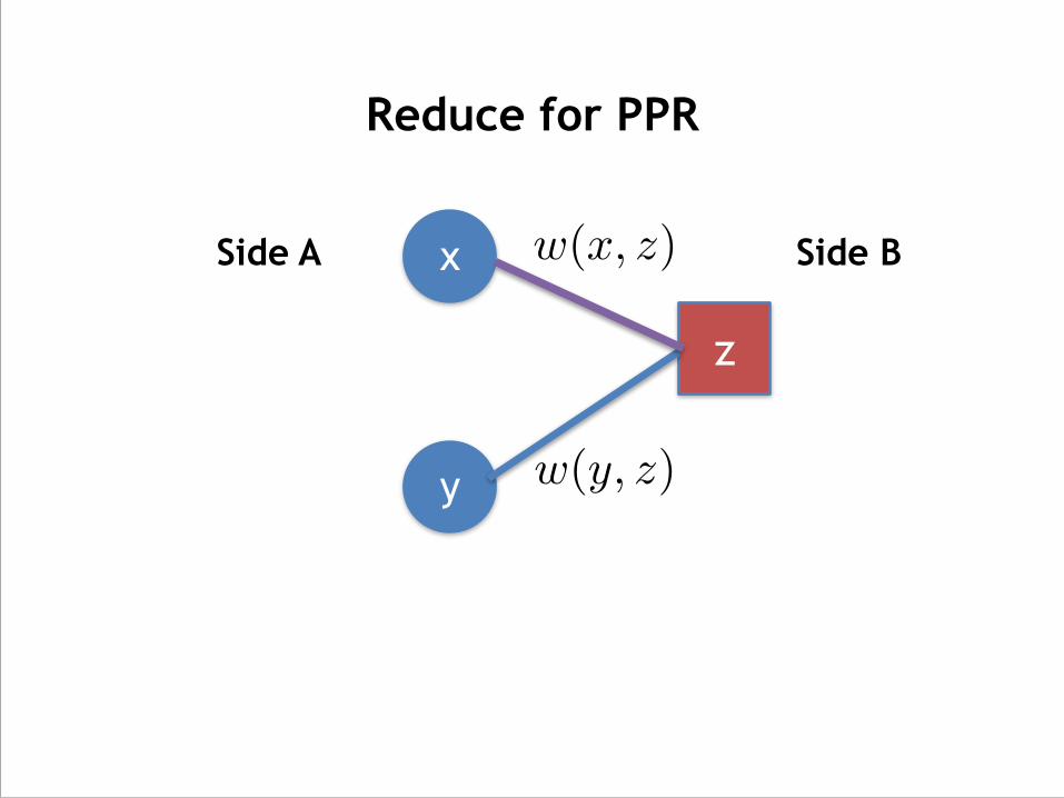
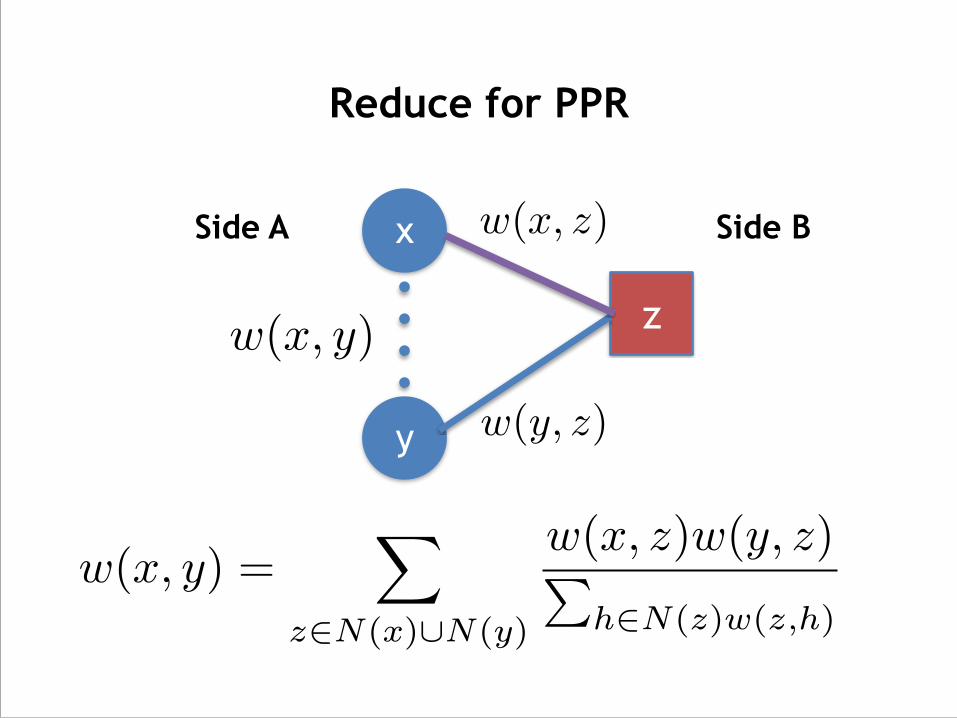
Reduce for PPR

y

x

z

Side A Side Bw(x, z)

w(y, z)

Reduce for PPR

y

x

z

Side A Side Bw(x, z)

w(y, z)

w(x, y)

w(x, y) =X

z2N(x)[N(y)

w(x, z)w(y, z)Ph2N(z)w(z,h)

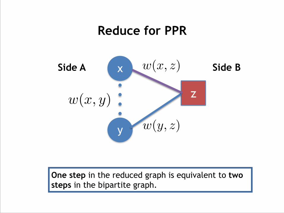
Reduce for PPR

y

x

z

One step in the reduced graph is equivalent to two steps in the bipartite graph.

w(x, z)

w(y, z)

w(x, y)

Side A Side B

Properties of the Reduced Graph

Lemma 1: PPR(G,↵, a)[A] = 12�↵PPR(G, 2↵� ↵2, a)

Proof Sketch: ● Every path between nodes in A is even. !

● Probability of not jumping for two steps. !● The probability of being in the A-Side at

stationarity does not depend on the graph.

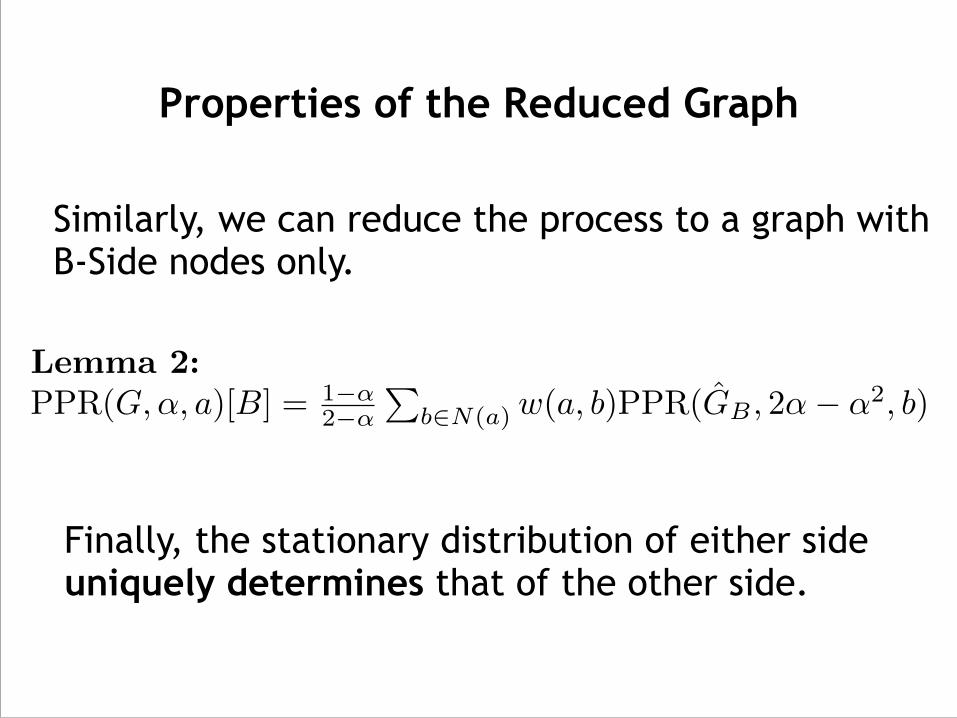
Properties of the Reduced Graph

Lemma 2:PPR(G,↵, a)[B] = 1�↵

2�↵

Pb2N(a) w(a, b)PPR(GB , 2↵� ↵2, b)

Similarly, we can reduce the process to a graph with B-Side nodes only.

Finally, the stationary distribution of either side uniquely determines that of the other side.

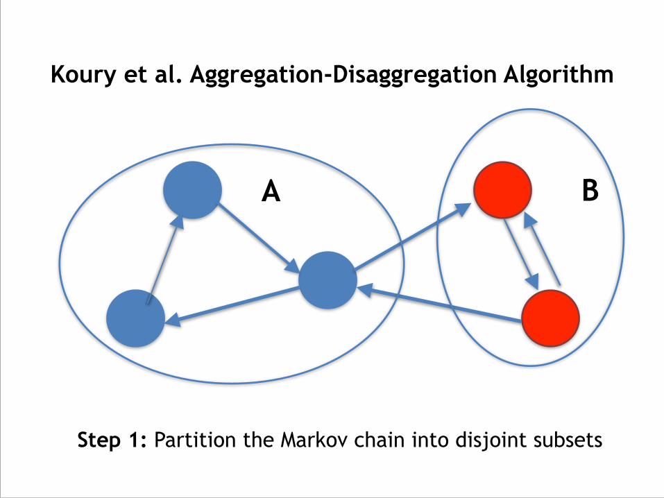
Koury et al. Aggregation-Disaggregation Algorithm

Step 1: Partition the Markov chain into disjoint subsets

A B

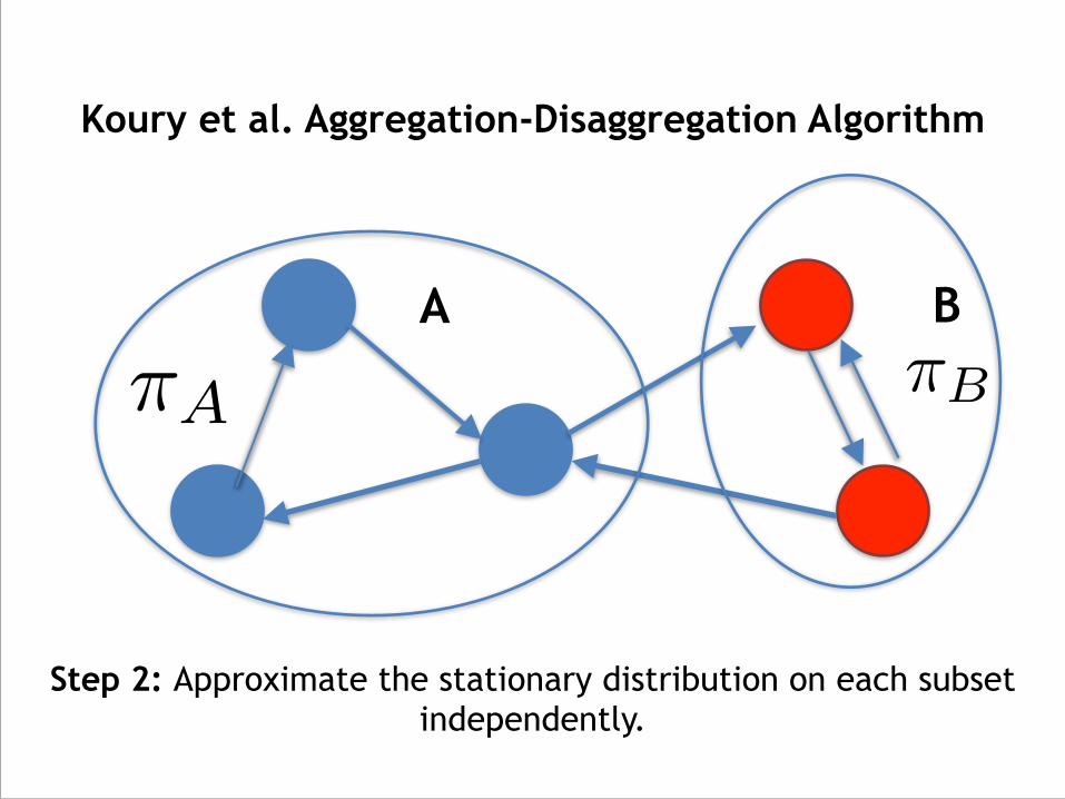
Koury et al. Aggregation-Disaggregation Algorithm

Step 2: Approximate the stationary distribution on each subset independently.

⇡A ⇡B

A B

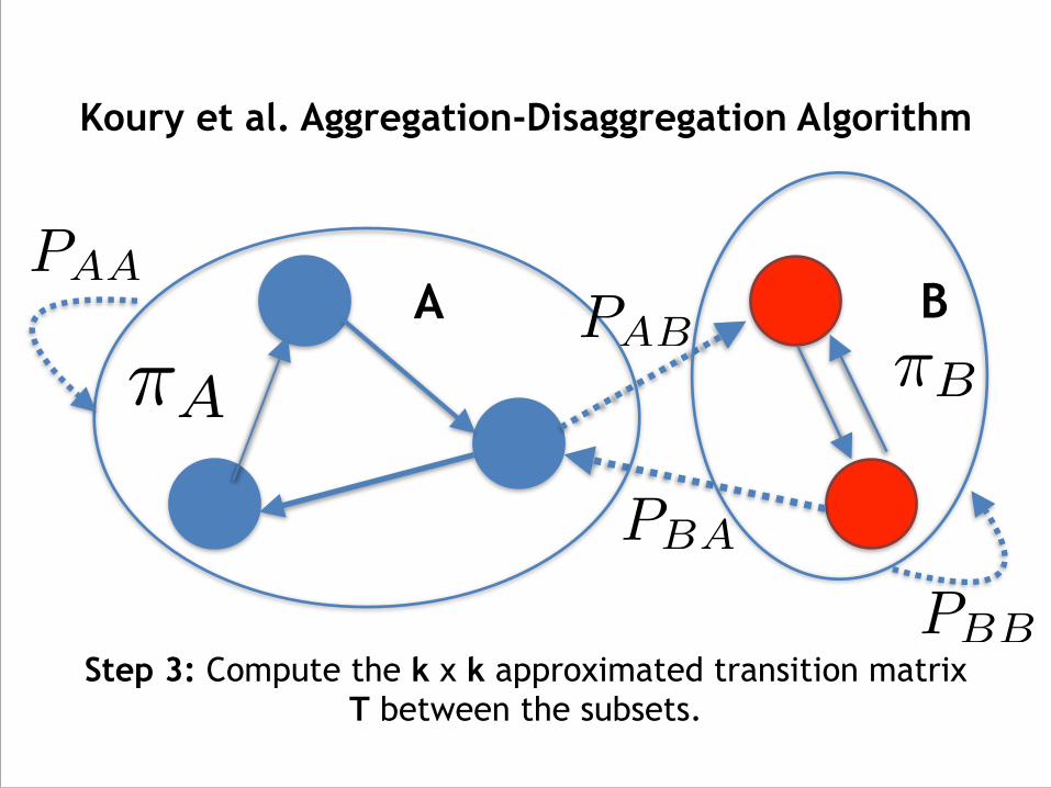
Koury et al. Aggregation-Disaggregation Algorithm

Step 3: Compute the k x k approximated transition matrix T between the subsets.

⇡A

PAB

PBA

PBB

PAAA B

⇡B

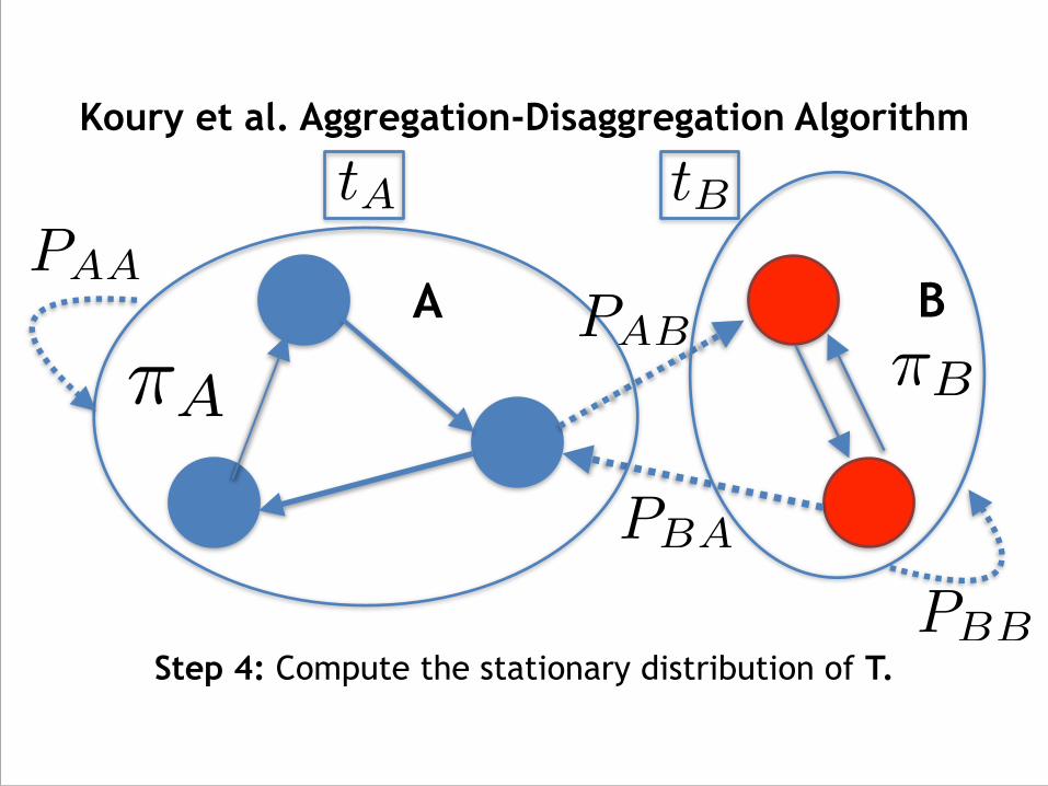
Koury et al. Aggregation-Disaggregation Algorithm

Step 4: Compute the stationary distribution of T.

⇡A

PAB

PBA

PBB

PAAA B

⇡B

tA tB

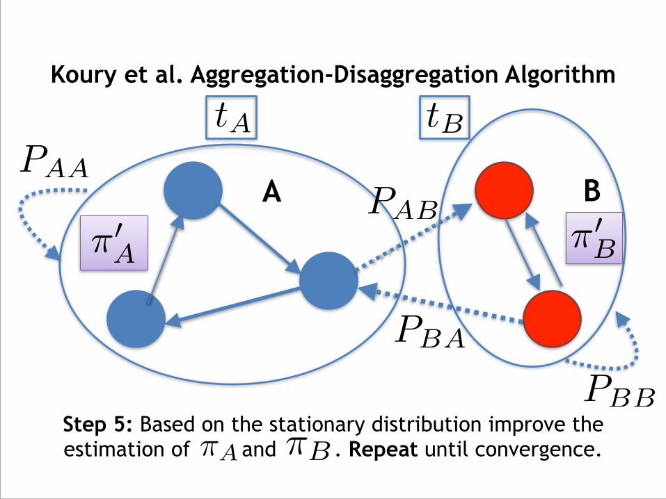
Koury et al. Aggregation-Disaggregation Algorithm

Step 5: Based on the stationary distribution improve the estimation of and . Repeat until convergence.

PAB

PBA

PBB

PAAA B

tA

⇡A ⇡B

tB

⇡0B⇡0

A

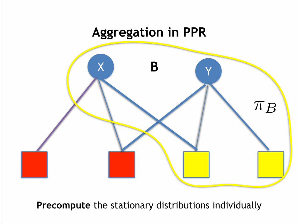
Aggregation in PPR

X Y

Precompute the stationary distributions individually

⇡A

A

Aggregation in PPR

X Y

Precompute the stationary distributions individually

⇡B

B

Aggregation in PPR

The two subsets are not disjoint!

A B

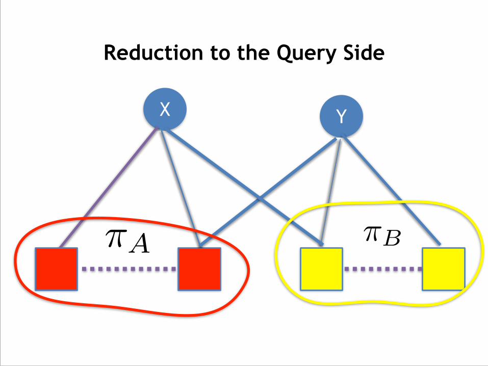
Reduction to the Query Side

X Y

⇡A ⇡B

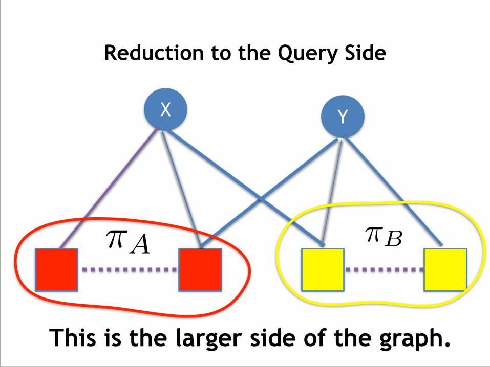
Reduction to the Query Side

X Y

This is the larger side of the graph.

⇡A ⇡B

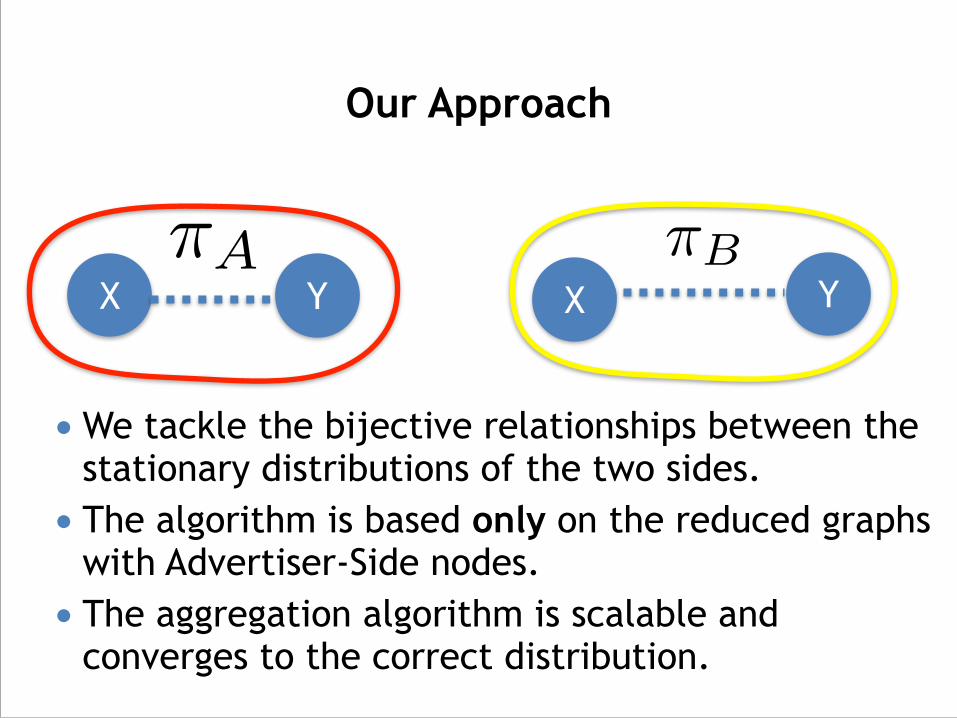
Our Approach

X Y X Y

● We tackle the bijective relationships between the stationary distributions of the two sides.

● The algorithm is based only on the reduced graphs with Advertiser-Side nodes.

● The aggregation algorithm is scalable and converges to the correct distribution.

⇡A ⇡B

Experimental Evaluation

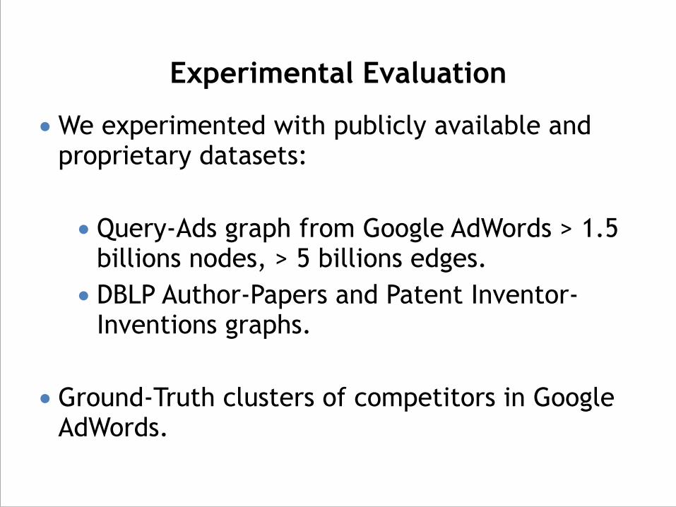
● We experimented with publicly available and proprietary datasets: !● Query-Ads graph from Google AdWords > 1.5

billions nodes, > 5 billions edges. ● DBLP Author-Papers and Patent Inventor-

Inventions graphs. !

● Ground-Truth clusters of competitors in Google AdWords.

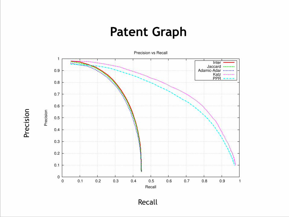
Patent Graph

Recall

Prec

isio

n

0

0.1

0.2

0.3

0.4

0.5

0.6

0.7

0.8

0.9

1

0 0.1 0.2 0.3 0.4 0.5 0.6 0.7 0.8 0.9 1

Pre

cis

ion

Recall

Precision vs Recall

InterJaccard

Adamic-AdarKatzPPR

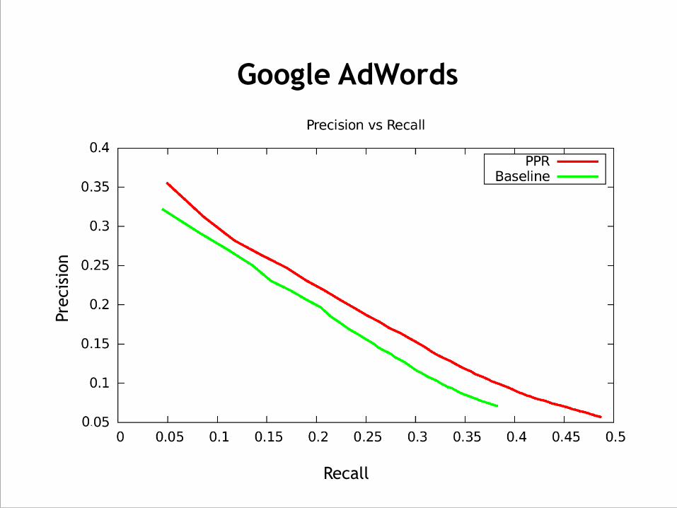
Google AdWords

Recall

Prec

isio

n

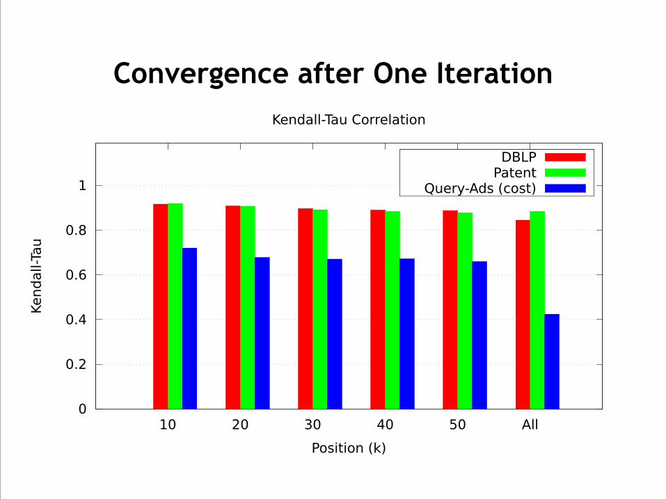
Convergence after One Iteration

��

����

����

����

����

��

�� �� � �� � ���

����������

������������

����������������������

� !�������

"���#������$����

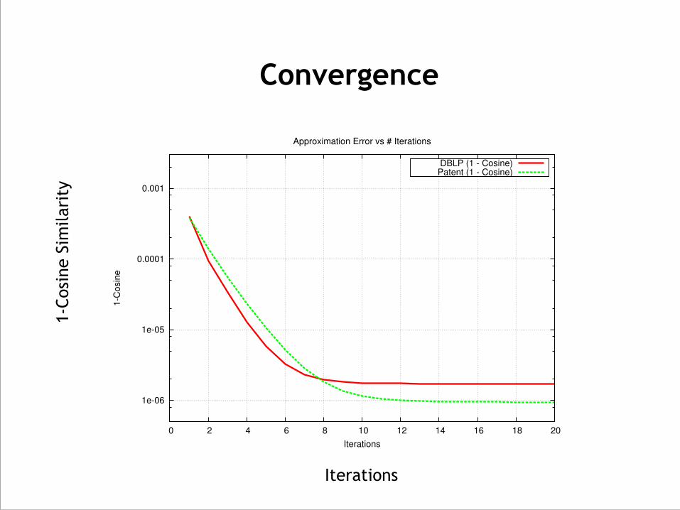
Convergence

Iterations

1-Co

sine

Sim

ilari

ty

1e-06

1e-05

0.0001

0.001

0 2 4 6 8 10 12 14 16 18 20

1-C

osin

e

Iterations

Approximation Error vs # Iterations

DBLP (1 - Cosine)Patent (1 - Cosine)

Conclusions and Future Work

● Good accuracy and fast convergence. !●The framework can be applied to other

problems and similarity measures. !●Future work could focus on the case

where categories are not disjoint is relevant.

Thank you for your attention