lable at ScienceDirect

Building and Environment 112 (2017) 250e260

Contents lists avai

Building and Environment

journal homepage: www.elsevier .com/locate/bui ldenv

Simple and accurate temperature correction for moisture pincalibrations in oriented strand board

C.R. Boardman*, Samuel V. Glass, Patricia K. LebowForest Products Laboratory, USA

a r t i c l e i n f o

Article history:Received 29 September 2016Received in revised form21 November 2016Accepted 22 November 2016Available online 24 November 2016

Keywords:Moisture pinOriented strand boardMoisture contentResistanceCalibrationTemperature

* Corresponding author. Forest Products LaboratoryPinchot Dr., Madison, WI 53726, USA.

E-mail address: cboardman@fs.fed.us (C.R. Boardm

http://dx.doi.org/10.1016/j.buildenv.2016.11.0390360-1323/Published by Elsevier Ltd.

a b s t r a c t

Oriented strand board (OSB) is commonly used in the residential construction market in North Americaand its moisture-related durability is a critical consideration for building envelope design. Measurementof OSB moisture content (MC), a key determinant of durability, is often done using moisture pins andrelies on a correlation between MC and the electrical resistance (R) of the OSB between the pins. Earlywork on these correlations focused on solid lumber and recent correlations for engineered woodproducts lack data regarding the temperature effects on R. We provide data on 1001 resistance mea-surements in OSB, sourced from three different locations, over a wide temperature (�17 �Ce70 �C) andrelative humidity (35%e95%) range. This data, in conjunction with gravimetric MC readings, is used totest existing correlations and support a new simple, accurate formula for calculating MC from resistanceand temperature measurements in OSB.

Published by Elsevier Ltd.

1. Introduction

Oriented strand board (OSB) structural panel sheathing hasbeen used in the North American residential construction marketfor several decades (see Zerbe [1] for a history of development).OSB has moisture transfer properties that differ from both plywoodand construction lumber [2,3]. Moisture-related durability is acritical consideration in building envelope design, particularlywhen insulation levels and airtightness of wall and roof assembliesare increased or new materials are introduced. Over the last 15years a large number of field studies in various North Americanclimates have monitored the hygrothermal performance of walland roof assemblies that include OSB sheathing [4e24]. Themoisture content (MC) of OSB sheathing is a key criterion forevaluation of field moisture performance. Moisture accumulationin wood-based materials can lead to mold growth, fungal decay,corrosion of embedded metal fasteners, expansion-contractiondamage, and loss of structural capacity. Development of mathe-matical models for some of these damage functions is the subject ofongoing research [25e35]. While mold growth depends on surfacewater activity (rather than bulk moisture content, though these are

, U.S. Forest Service, 1 Gifford

an).

related), the other types of damage are dependent on moisturecontent. For example a common rule of thumb suggests keepingwood products below 20%MC tominimize risk of decay [36e38]. Inaddition, questions about moisture risk have driven the ongoinginterest in validation and tuning of hygrothermal models as well asparametric analysis [39e48] which allow the prediction of OSBmoisture performance during the design of building envelope as-semblies. Verification of the models depends on accurate mea-surement of MC in field and laboratory studies to compare tomodelprediction.

A common method for measuring moisture content of woodproducts in the field is through use of a moisture meter, whichallows immediate spot readings, or installation of moisture pinswith a data acquisition system for long term monitoring. Otherresearchers rely on direct gravimetric measurement which requiresobtaining the mass of a wood sample before and after oven drying.Direct measurement, however, can be cumbersome in practicewhen applied to field experiments as it relies on either cutting out aspecimen or inserting and removing a wood plug from a location inthe assembly that may not be readily accessible [49]. While highlyaccurate, the method is labor intensive andmay limit the frequencyand extent of data collection. But it does find use in laboratorystudies such as [50] which also illustrates the use of OSB outside theNorth American context as an interior vapor retarder. So whiledirect gravimetric measurement has its place, and OSB can be used

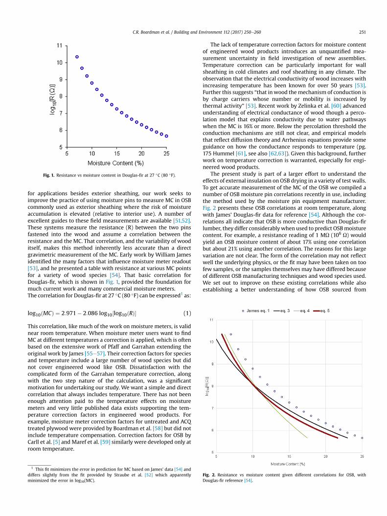
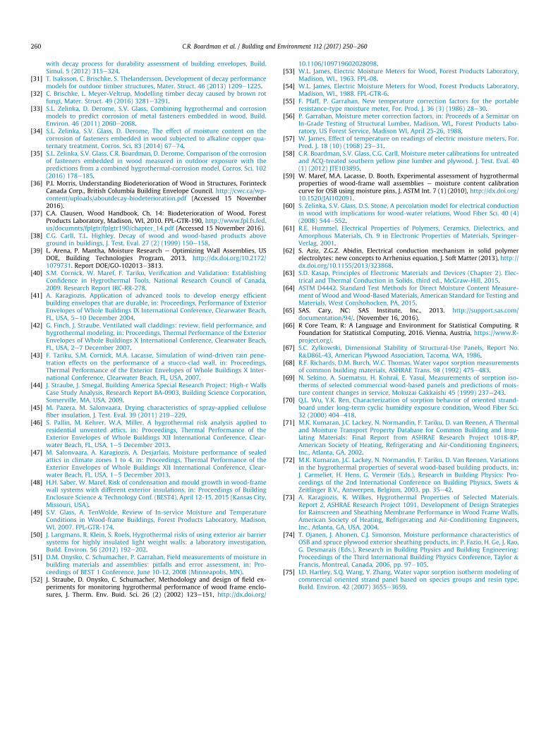
Fig. 1. Resistance vs moisture content in Douglas-fir at 27 �C (80 �F).

C.R. Boardman et al. / Building and Environment 112 (2017) 250e260 251

for applications besides exterior sheathing, our work seeks toimprove the practice of using moisture pins to measure MC in OSBcommonly used as exterior sheathing where the risk of moistureaccumulation is elevated (relative to interior use). A number ofexcellent guides to these field measurements are available [51,52].These systems measure the resistance (R) between the two pinsfastened into the wood and assume a correlation between theresistance and the MC. That correlation, and the variability of wooditself, makes this method inherently less accurate than a directgravimetric measurement of the MC. Early work by William Jamesidentified the many factors that influence moisture meter readout[53], and he presented a table with resistance at various MC pointsfor a variety of wood species [54]. That basic correlation forDouglas-fir, which is shown in Fig. 1, provided the foundation formuch current work and many commercial moisture meters.The correlation for Douglas-fir at 27 �C (80 �F) can be expressed1 as:

log10ðMCÞ ¼ 2:971� 2:086 log10½log10ðRÞ� (1)

This correlation, like much of the work on moisture meters, is validnear room temperature. When moisture meter users want to findMC at different temperatures a correction is applied, which is oftenbased on the extensive work of Pfaff and Garrahan extending theoriginal work by James [55e57]. Their correction factors for speciesand temperature include a large number of wood species but didnot cover engineered wood like OSB. Dissatisfaction with thecomplicated form of the Garrahan temperature correction, alongwith the two step nature of the calculation, was a significantmotivation for undertaking our study. We want a simple and directcorrelation that always includes temperature. There has not beenenough attention paid to the temperature effects on moisturemeters and very little published data exists supporting the tem-perature correction factors in engineered wood products. Forexample, moisture meter correction factors for untreated and ACQtreated plywood were provided by Boardman et al. [58] but did notinclude temperature compensation. Correction factors for OSB byCarll et al. [5] and Maref et al. [59] similarly were developed only atroom temperature.

1 This fit minimizes the error in prediction for MC based on James' data [54] anddiffers slightly from the fit provided by Straube et al. [52] which apparentlyminimized the error in log10(MC).

The lack of temperature correction factors for moisture contentof engineered wood products introduces an unquantified mea-surement uncertainty in field investigation of new assemblies.Temperature correction can be particularly important for wallsheathing in cold climates and roof sheathing in any climate. Theobservation that the electrical conductivity of wood increases withincreasing temperature has been known for over 50 years [53].Further this suggests “that inwood the mechanism of conduction isby charge carriers whose number or mobility is increased bythermal activity” [53]. Recent work by Zelinka et al. [60] advancedunderstanding of electrical conductance of wood though a perco-lation model that explains conductivity due to water pathwayswhen the MC is 16% or more. Below the percolation threshold theconduction mechanisms are still not clear, and empirical modelsthat reflect diffusion theory and Arrhenius equations provide someguidance on how the conductance responds to temperature (pg.175 Hummel [61], see also [62,63]). Given this background, furtherwork on temperature correction is warranted, especially for engi-neered wood products.

The present study is part of a larger effort to understand theeffects of external insulation on OSB drying in a variety of test walls.To get accurate measurement of the MC of the OSB we compiled anumber of OSB moisture pin correlations recently in use, includingthe method used by the moisture pin equipment manufacturer.Fig. 2 presents these OSB correlations at room temperature, alongwith James' Douglas-fir data for reference [54]. Although the cor-relations all indicate that OSB is more conductive than Douglas-firlumber, they differ considerablywhen used to predict OSBmoisturecontent. For example, a resistance reading of 1 MU (106 U) wouldyield an OSB moisture content of about 17% using one correlationbut about 21% using another correlation. The reasons for this largevariation are not clear. The form of the correlation may not reflectwell the underlying physics, or the fit may have been taken on toofew samples, or the samples themselves may have differed becauseof different OSB manufacturing techniques and wood species used.We set out to improve on these existing correlations while alsoestablishing a better understanding of how OSB sourced from

Fig. 2. Resistance vs moisture content given different correlations for OSB, withDouglas-fir reference [54].

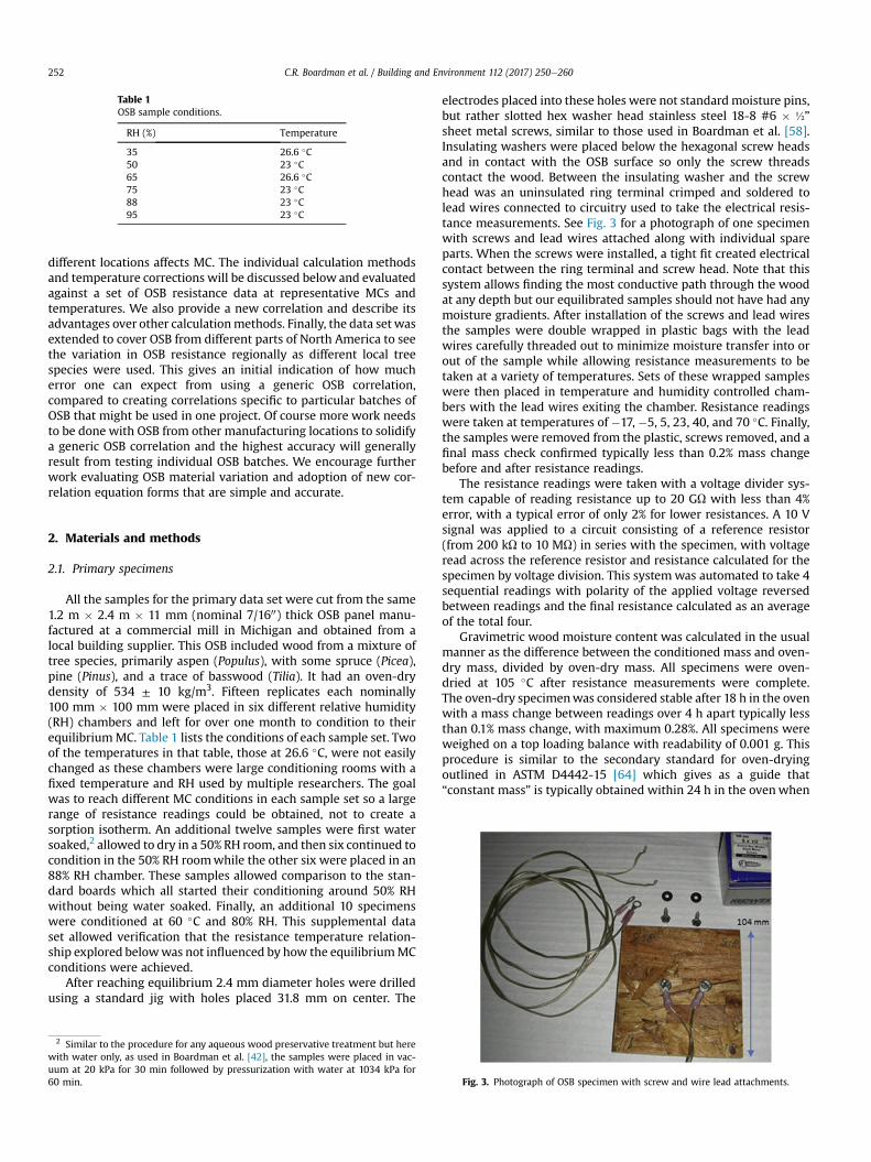
Table 1OSB sample conditions.

RH (%) Temperature

35 26.6 �C50 23 �C65 26.6 �C75 23 �C88 23 �C95 23 �C

C.R. Boardman et al. / Building and Environment 112 (2017) 250e260252

different locations affects MC. The individual calculation methodsand temperature corrections will be discussed below and evaluatedagainst a set of OSB resistance data at representative MCs andtemperatures. We also provide a new correlation and describe itsadvantages over other calculationmethods. Finally, the data set wasextended to cover OSB from different parts of North America to seethe variation in OSB resistance regionally as different local treespecies were used. This gives an initial indication of how mucherror one can expect from using a generic OSB correlation,compared to creating correlations specific to particular batches ofOSB that might be used in one project. Of course more work needsto be done with OSB from other manufacturing locations to solidifya generic OSB correlation and the highest accuracy will generallyresult from testing individual OSB batches. We encourage furtherwork evaluating OSB material variation and adoption of new cor-relation equation forms that are simple and accurate.

2. Materials and methods

2.1. Primary specimens

All the samples for the primary data set were cut from the same1.2 m � 2.4 m � 11 mm (nominal 7/1600) thick OSB panel manu-factured at a commercial mill in Michigan and obtained from alocal building supplier. This OSB included wood from a mixture oftree species, primarily aspen (Populus), with some spruce (Picea),pine (Pinus), and a trace of basswood (Tilia). It had an oven-drydensity of 534 ± 10 kg/m3. Fifteen replicates each nominally100 mm � 100 mm were placed in six different relative humidity(RH) chambers and left for over one month to condition to theirequilibriumMC. Table 1 lists the conditions of each sample set. Twoof the temperatures in that table, those at 26.6 �C, were not easilychanged as these chambers were large conditioning rooms with afixed temperature and RH used by multiple researchers. The goalwas to reach different MC conditions in each sample set so a largerange of resistance readings could be obtained, not to create asorption isotherm. An additional twelve samples were first watersoaked,2 allowed to dry in a 50% RH room, and then six continued tocondition in the 50% RH roomwhile the other six were placed in an88% RH chamber. These samples allowed comparison to the stan-dard boards which all started their conditioning around 50% RHwithout being water soaked. Finally, an additional 10 specimenswere conditioned at 60 �C and 80% RH. This supplemental dataset allowed verification that the resistance temperature relation-ship explored belowwas not influenced by how the equilibriumMCconditions were achieved.

After reaching equilibrium 2.4 mm diameter holes were drilledusing a standard jig with holes placed 31.8 mm on center. The

2 Similar to the procedure for any aqueous wood preservative treatment but herewith water only, as used in Boardman et al. [42], the samples were placed in vac-uum at 20 kPa for 30 min followed by pressurization with water at 1034 kPa for60 min.

electrodes placed into these holes were not standardmoisture pins,but rather slotted hex washer head stainless steel 18-8 #6 � ½”

sheet metal screws, similar to those used in Boardman et al. [58].Insulating washers were placed below the hexagonal screw headsand in contact with the OSB surface so only the screw threadscontact the wood. Between the insulating washer and the screwhead was an uninsulated ring terminal crimped and soldered tolead wires connected to circuitry used to take the electrical resis-tance measurements. See Fig. 3 for a photograph of one specimenwith screws and lead wires attached along with individual spareparts. When the screws were installed, a tight fit created electricalcontact between the ring terminal and screw head. Note that thissystem allows finding the most conductive path through the woodat any depth but our equilibrated samples should not have had anymoisture gradients. After installation of the screws and lead wiresthe samples were double wrapped in plastic bags with the leadwires carefully threaded out to minimize moisture transfer into orout of the sample while allowing resistance measurements to betaken at a variety of temperatures. Sets of these wrapped sampleswere then placed in temperature and humidity controlled cham-bers with the lead wires exiting the chamber. Resistance readingswere taken at temperatures of �17, �5, 5, 23, 40, and 70 �C. Finally,the samples were removed from the plastic, screws removed, and afinal mass check confirmed typically less than 0.2% mass changebefore and after resistance readings.

The resistance readings were taken with a voltage divider sys-tem capable of reading resistance up to 20 GU with less than 4%error, with a typical error of only 2% for lower resistances. A 10 Vsignal was applied to a circuit consisting of a reference resistor(from 200 kU to 10 MU) in series with the specimen, with voltageread across the reference resistor and resistance calculated for thespecimen by voltage division. This systemwas automated to take 4sequential readings with polarity of the applied voltage reversedbetween readings and the final resistance calculated as an averageof the total four.

Gravimetric wood moisture content was calculated in the usualmanner as the difference between the conditioned mass and oven-dry mass, divided by oven-dry mass. All specimens were oven-dried at 105 �C after resistance measurements were complete.The oven-dry specimenwas considered stable after 18 h in the ovenwith a mass change between readings over 4 h apart typically lessthan 0.1% mass change, with maximum 0.28%. All specimens wereweighed on a top loading balance with readability of 0.001 g. Thisprocedure is similar to the secondary standard for oven-dryingoutlined in ASTM D4442-15 [64] which gives as a guide that“constant mass” is typically obtained within 24 h in the ovenwhen

Fig. 3. Photograph of OSB specimen with screw and wire lead attachments.

C.R. Boardman et al. / Building and Environment 112 (2017) 250e260 253

no appreciable change is noted in final mass at approximately 4 hintervals. In our case the typical change observed limits the MCaccuracy to 0.2% and could not be improved without the muchstricter mass measurement requirements in the primary standard.

2.2. Secondary specimens

Samples for the secondary data set were cut from 11 mm(nominal 7/1600) OSB sourced from Texas and British Columbiamills. Texas OSB samples were made from primarily southern yel-low pine wood, and had an oven-dry density of 564 ± 19 kg/m3.British Columbia OSB samples were made from primarily aspenwood (Populus), and had an oven-dry density of 565 ± 49 kg/m3. Sixreplicates from each locationwere placed in the same conditions asTable 1 and prepared for resistance readings in the same manner asthe primary data set. The temperatures sampled included �17, �5,5, 10, 23, 40, and 60 �C. The 10 �C reading was added to be the lowertemperature reading for the 50% RH readings. Very dry and coldsamples reach resistance values too high for our equipment tomeasure reliably. The high temperature was reduced from 70 to

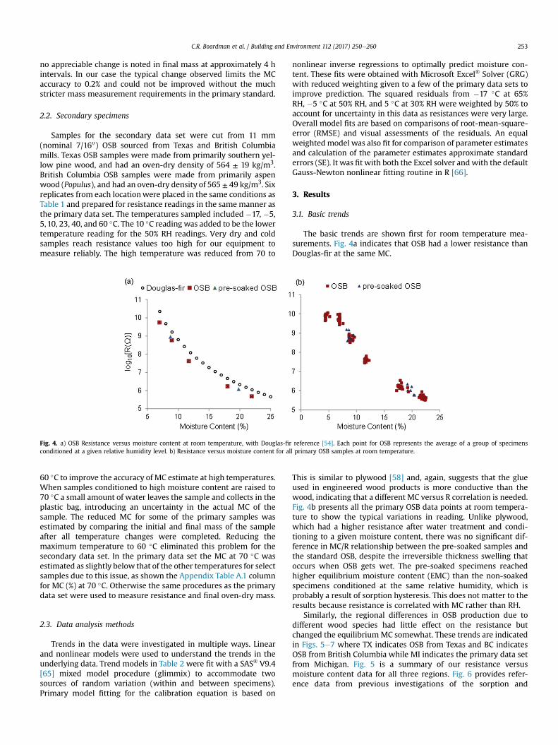
Fig. 4. a) OSB Resistance versus moisture content at room temperature, with Douglas-fir reference [54]. Each point for OSB represents the average of a group of specimensconditioned at a given relative humidity level. b) Resistance versus moisture content for all primary OSB samples at room temperature.

60 �C to improve the accuracy of MC estimate at high temperatures.When samples conditioned to high moisture content are raised to70 �C a small amount of water leaves the sample and collects in theplastic bag, introducing an uncertainty in the actual MC of thesample. The reduced MC for some of the primary samples wasestimated by comparing the initial and final mass of the sampleafter all temperature changes were completed. Reducing themaximum temperature to 60 �C eliminated this problem for thesecondary data set. In the primary data set the MC at 70 �C wasestimated as slightly below that of the other temperatures for selectsamples due to this issue, as shown the Appendix Table A.1 columnfor MC (%) at 70 �C. Otherwise the same procedures as the primarydata set were used to measure resistance and final oven-dry mass.

2.3. Data analysis methods

Trends in the data were investigated in multiple ways. Linearand nonlinear models were used to understand the trends in theunderlying data. Trend models in Table 2 were fit with a SAS® V9.4[65] mixed model procedure (glimmix) to accommodate twosources of random variation (within and between specimens).Primary model fitting for the calibration equation is based on

nonlinear inverse regressions to optimally predict moisture con-tent. These fits were obtained with Microsoft Excel® Solver (GRG)with reduced weighting given to a few of the primary data sets toimprove prediction. The squared residuals from �17 �C at 65%RH, �5 �C at 50% RH, and 5 �C at 30% RH were weighted by 50% toaccount for uncertainty in this data as resistances were very large.Overall model fits are based on comparisons of root-mean-square-error (RMSE) and visual assessments of the residuals. An equalweightedmodel was also fit for comparison of parameter estimatesand calculation of the parameter estimates approximate standarderrors (SE). It was fit with both the Excel solver and with the defaultGauss-Newton nonlinear fitting routine in R [66].

3. Results

3.1. Basic trends

The basic trends are shown first for room temperature mea-surements. Fig. 4a indicates that OSB had a lower resistance thanDouglas-fir at the same MC.

This is similar to plywood [58] and, again, suggests that the glueused in engineered wood products is more conductive than thewood, indicating that a different MC versus R correlation is needed.Fig. 4b presents all the primary OSB data points at room tempera-ture to show the typical variations in reading. Unlike plywood,which had a higher resistance after water treatment and condi-tioning to a given moisture content, there was no significant dif-ference in MC/R relationship between the pre-soaked samples andthe standard OSB, despite the irreversible thickness swelling thatoccurs when OSB gets wet. The pre-soaked specimens reachedhigher equilibrium moisture content (EMC) than the non-soakedspecimens conditioned at the same relative humidity, which isprobably a result of sorption hysteresis. This does not matter to theresults because resistance is correlated with MC rather than RH.

Similarly, the regional differences in OSB production due todifferent wood species had little effect on the resistance butchanged the equilibrium MC somewhat. These trends are indicatedin Figs. 5e7 where TX indicates OSB from Texas and BC indicatesOSB from British Columbia while MI indicates the primary data setfrom Michigan. Fig. 5 is a summary of our resistance versusmoisture content data for all three regions. Fig. 6 provides refer-ence data from previous investigations of the sorption and

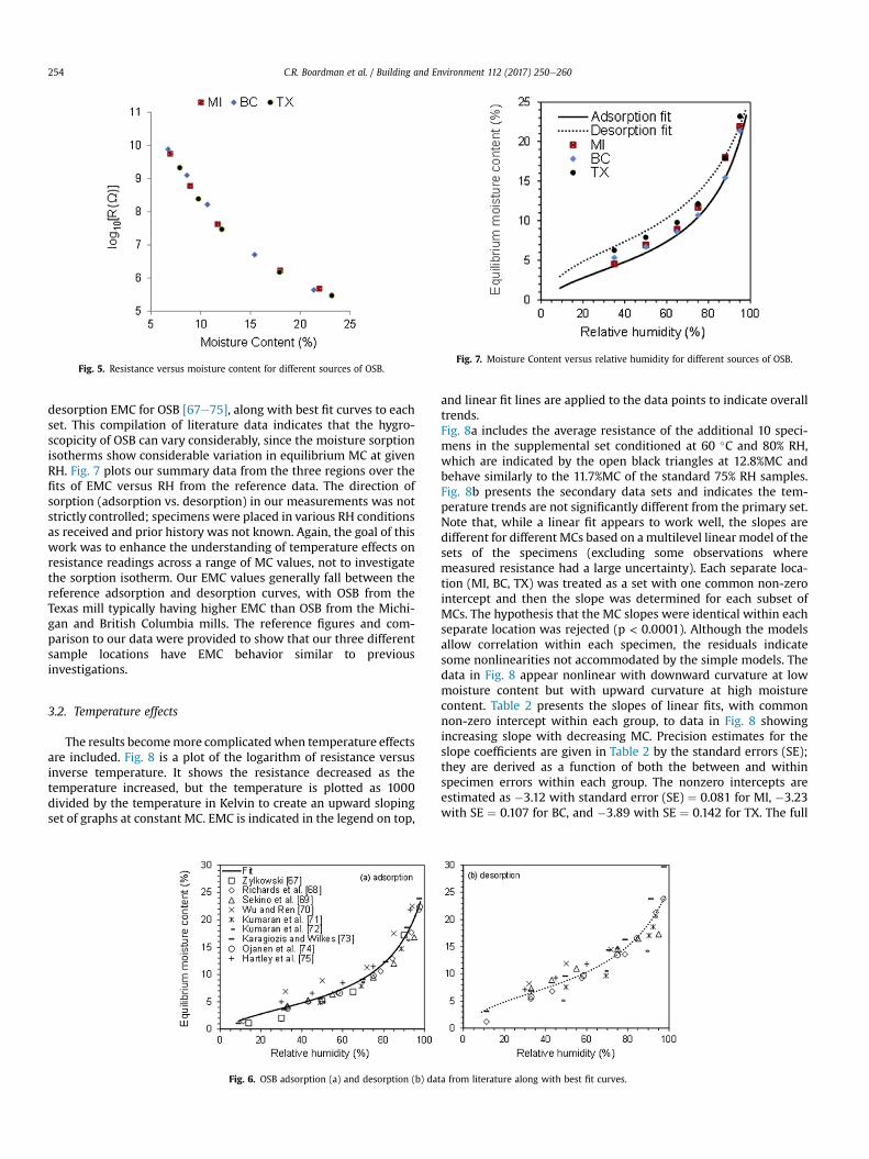
Fig. 5. Resistance versus moisture content for different sources of OSB.Fig. 7. Moisture Content versus relative humidity for different sources of OSB.

C.R. Boardman et al. / Building and Environment 112 (2017) 250e260254

desorption EMC for OSB [67e75], along with best fit curves to eachset. This compilation of literature data indicates that the hygro-scopicity of OSB can vary considerably, since the moisture sorptionisotherms show considerable variation in equilibrium MC at givenRH. Fig. 7 plots our summary data from the three regions over thefits of EMC versus RH from the reference data. The direction ofsorption (adsorption vs. desorption) in our measurements was notstrictly controlled; specimens were placed in various RH conditionsas received and prior history was not known. Again, the goal of thiswork was to enhance the understanding of temperature effects onresistance readings across a range of MC values, not to investigatethe sorption isotherm. Our EMC values generally fall between thereference adsorption and desorption curves, with OSB from theTexas mill typically having higher EMC than OSB from the Michi-gan and British Columbia mills. The reference figures and com-parison to our data were provided to show that our three differentsample locations have EMC behavior similar to previousinvestigations.

3.2. Temperature effects

The results becomemore complicatedwhen temperature effectsare included. Fig. 8 is a plot of the logarithm of resistance versusinverse temperature. It shows the resistance decreased as thetemperature increased, but the temperature is plotted as 1000divided by the temperature in Kelvin to create an upward slopingset of graphs at constant MC. EMC is indicated in the legend on top,

Fig. 6. OSB adsorption (a) and desorption (b) da

and linear fit lines are applied to the data points to indicate overalltrends.Fig. 8a includes the average resistance of the additional 10 speci-mens in the supplemental set conditioned at 60 �C and 80% RH,which are indicated by the open black triangles at 12.8%MC andbehave similarly to the 11.7%MC of the standard 75% RH samples.Fig. 8b presents the secondary data sets and indicates the tem-perature trends are not significantly different from the primary set.Note that, while a linear fit appears to work well, the slopes aredifferent for different MCs based on amultilevel linear model of thesets of the specimens (excluding some observations wheremeasured resistance had a large uncertainty). Each separate loca-tion (MI, BC, TX) was treated as a set with one common non-zerointercept and then the slope was determined for each subset ofMCs. The hypothesis that the MC slopes were identical within eachseparate location was rejected (p < 0.0001). Although the modelsallow correlation within each specimen, the residuals indicatesome nonlinearities not accommodated by the simple models. Thedata in Fig. 8 appear nonlinear with downward curvature at lowmoisture content but with upward curvature at high moisturecontent. Table 2 presents the slopes of linear fits, with commonnon-zero intercept within each group, to data in Fig. 8 showingincreasing slope with decreasing MC. Precision estimates for theslope coefficients are given in Table 2 by the standard errors (SE);they are derived as a function of both the between and withinspecimen errors within each group. The nonzero intercepts areestimated as �3.12 with standard error (SE) ¼ 0.081 for MI, �3.23with SE ¼ 0.107 for BC, and �3.89 with SE ¼ 0.142 for TX. The full

ta from literature along with best fit curves.

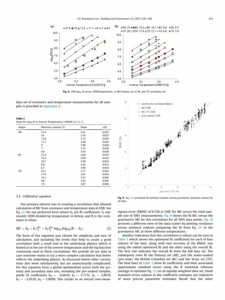
Fig. 8. OSB log10 R versus 1000/temperature. a) MI Primary set, b) BC and TX secondary set.

C.R. Boardman et al. / Building and Environment 112 (2017) 250e260 255

data set of resistance and temperature measurements for all sam-ples is provided in Appendix A.

Fig. 9. Eq. (2) correlation fit moisture content versus gravimetric moisture content forall data.

Table 2Slope for log10 R vs Inverse Temperature (1000/K) in Fig. 8.

Origin Moisture content (%) Slope ±SE

MI 21.9 2.61 0.02518 2.78 0.02512.8 3.13 0.02611.7 3.20 0.0259 3.48 0.0267 3.75 0.0264.6 3.93 0.028

BC 21.4 2.64 0.03215.4 2.99 0.03210.7 3.38 0.0338.8 3.63 0.0336.7 3.86 0.034

TX 23.1 2.77 0.04317.9 3.01 0.04312.1 3.37 0.0459.8 3.63 0.0457.9 3.87 0.046

3.3. Calibration equation

Our primary interest was in creating a correlation that allowedcalculation of MC from resistance and temperature data in OSB. SeeEq. (2) for our preferred form where bx are fit coefficients, Tf rep-resents 1000 divided by temperature in Kelvin, and R is the resis-tance in ohms.

MC ¼ b0 þ b1Tb4f þ b3T

b4f log10½log10ðRÞ � b2� (2)

The form of this equation was chosen for simplicity and ease ofcalculation, just including the terms that help to create a goodcorrelation with a small nod to the underlying physics which ishinted at in the use of the inverse temperature and the log functioncommonly used in these correlations. We provide all our data incase someone wants to try a more complex calculation that betterreflects the underlying physics. As discussed below other correla-tions also work satisfactorily, but are unnecessarily complicated.For this equation form a global optimization across both the pri-mary and secondary data sets, including the pre-soaked samples,yields fit coefficients b0 ¼ �8.6810, b1 ¼ 3.7172, b2 ¼ 3.8974,b3 ¼ �2.9129, b4 ¼ 1.9000. This results in an overall root-mean-

square-error (RMSE) of 0.726 in %MC for MC across the total sam-ple size of 1001 measurements. Fig. 9 shows the fit MC versus thegravimetric MC for this correlation for all 1001 data points. Fig. 10presents a different view of the data scatter by plotting resistanceversus moisture content comparing the fit from Eq. (2) to thegravimetric MC at three different temperatures.

Another indication that this correlation is robust can be seen inTable 3 which shows the optimized fit coefficients for each of foursubsets of the data, along with two versions of the RMSE, oneusing the subset optimized fit and the other using the overall fit.The first row indicates the overall fit from the full data set. Thesubsequent rows fit the Primary set (MI), just the water-soaked(pre-soak), the British Columbia set (BC) and the Texas set (TX).The final lines in Table 3 show fit coefficients and their associatedapproximate standard errors using the R statistical softwarepackage to optimize Eq. (2) on an equally weighted data set. Smallstandard errors relative to the coefficient estimates are indicativeof more precise parameter estimates. Recall that the other

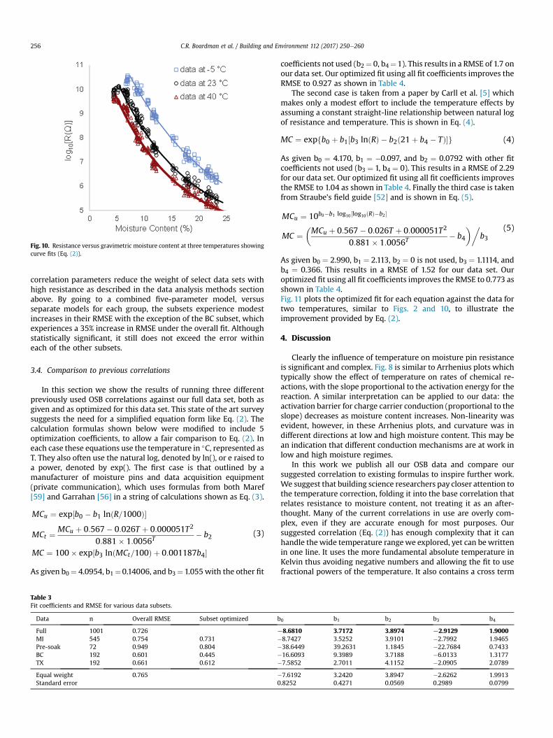
Fig. 10. Resistance versus gravimetric moisture content at three temperatures showingcurve fits (Eq. (2)).

C.R. Boardman et al. / Building and Environment 112 (2017) 250e260256

correlation parameters reduce the weight of select data sets withhigh resistance as described in the data analysis methods sectionabove. By going to a combined five-parameter model, versusseparate models for each group, the subsets experience modestincreases in their RMSE with the exception of the BC subset, whichexperiences a 35% increase in RMSE under the overall fit. Althoughstatistically significant, it still does not exceed the error withineach of the other subsets.

3.4. Comparison to previous correlations

In this section we show the results of running three differentpreviously used OSB correlations against our full data set, both asgiven and as optimized for this data set. This state of the art surveysuggests the need for a simplified equation form like Eq. (2). Thecalculation formulas shown below were modified to include 5optimization coefficients, to allow a fair comparison to Eq. (2). Ineach case these equations use the temperature in �C, represented asT. They also often use the natural log, denoted by ln(), or e raised toa power, denoted by exp(). The first case is that outlined by amanufacturer of moisture pins and data acquisition equipment(private communication), which uses formulas from both Maref[59] and Garrahan [56] in a string of calculations shown as Eq. (3).

MCu ¼ exp½b0 � b1 lnðR=1000Þ�

MCt ¼ MCu þ 0:567� 0:026T þ 0:000051T2

0:881� 1:0056T� b2

MC ¼ 100� exp½b3 lnðMCt=100Þ þ 0:001187b4�

(3)

As given b0¼ 4.0954, b1¼0.14006, and b3¼ 1.055with the other fit

Table 3Fit coefficients and RMSE for various data subsets.

Data n Overall RMSE Subset optimized b

Full 1001 0.726 ¡MI 545 0.754 0.731 �Pre-soak 72 0.949 0.804 �BC 192 0.601 0.445 �TX 192 0.661 0.612 �Equal weight 0.765 �Standard error 0

coefficients not used (b2¼ 0, b4¼1). This results in a RMSE of 1.7 onour data set. Our optimized fit using all fit coefficients improves theRMSE to 0.927 as shown in Table 4.

The second case is taken from a paper by Carll et al. [5] whichmakes only a modest effort to include the temperature effects byassuming a constant straight-line relationship between natural logof resistance and temperature. This is shown in Eq. (4).

MC ¼ expfb0 þ b1½b3 lnðRÞ � b2ð21þ b4 � TÞ�g (4)

As given b0 ¼ 4.170, b1 ¼ �0.097, and b2 ¼ 0.0792 with other fitcoefficients not used (b3 ¼ 1, b4 ¼ 0). This results in a RMSE of 2.29for our data set. Our optimized fit using all fit coefficients improvesthe RMSE to 1.04 as shown in Table 4. Finally the third case is takenfrom Straube's field guide [52] and is shown in Eq. (5).

MCu ¼ 10b0�b1 log10½log10ðRÞ�b2 �

MC ¼�MCu þ 0:567� 0:026T þ 0:000051T2

0:881� 1:0056T� b4

��b3

(5)

As given b0 ¼ 2.990, b1 ¼ 2.113, b2 ¼ 0 is not used, b3 ¼ 1.1114, andb4 ¼ 0.366. This results in a RMSE of 1.52 for our data set. Ouroptimized fit using all fit coefficients improves the RMSE to 0.773 asshown in Table 4.Fig. 11 plots the optimized fit for each equation against the data fortwo temperatures, similar to Figs. 2 and 10, to illustrate theimprovement provided by Eq. (2).

4. Discussion

Clearly the influence of temperature on moisture pin resistanceis significant and complex. Fig. 8 is similar to Arrhenius plots whichtypically show the effect of temperature on rates of chemical re-actions, with the slope proportional to the activation energy for thereaction. A similar interpretation can be applied to our data: theactivation barrier for charge carrier conduction (proportional to theslope) decreases as moisture content increases. Non-linearity wasevident, however, in these Arrhenius plots, and curvature was indifferent directions at low and high moisture content. This may bean indication that different conduction mechanisms are at work inlow and high moisture regimes.

In this work we publish all our OSB data and compare oursuggested correlation to existing formulas to inspire further work.We suggest that building science researchers pay closer attention tothe temperature correction, folding it into the base correlation thatrelates resistance to moisture content, not treating it as an after-thought. Many of the current correlations in use are overly com-plex, even if they are accurate enough for most purposes. Oursuggested correlation (Eq. (2)) has enough complexity that it canhandle the wide temperature rangewe explored, yet can bewrittenin one line. It uses the more fundamental absolute temperature inKelvin thus avoiding negative numbers and allowing the fit to usefractional powers of the temperature. It also contains a cross term

0 b1 b2 b3 b4

8.6810 3.7172 3.8974 ¡2.9129 1.90008.7427 3.5252 3.9101 �2.7992 1.946538.6449 39.2631 1.1845 �22.7684 0.743316.6093 9.3989 3.7188 �6.0133 1.31777.5852 2.7011 4.1152 �2.0905 2.0789

7.6192 3.2420 3.8947 �2.6262 1.9913.8252 0.4271 0.0569 0.2989 0.0799

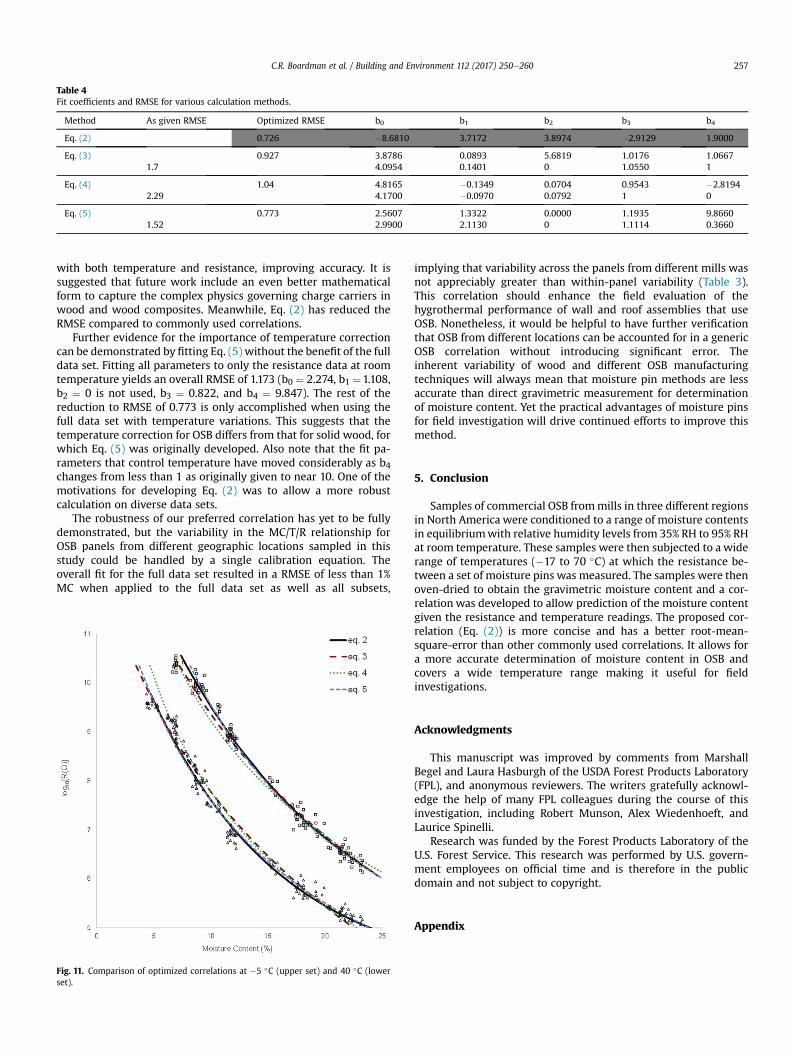
Table 4Fit coefficients and RMSE for various calculation methods.

Method As given RMSE Optimized RMSE b0 b1 b2 b3 b4

Eq. (2) 0.726 �8.6810 3.7172 3.8974 �2.9129 1.9000

Eq. (3) 0.927 3.8786 0.0893 5.6819 1.0176 1.06671.7 4.0954 0.1401 0 1.0550 1

Eq. (4) 1.04 4.8165 �0.1349 0.0704 0.9543 �2.81942.29 4.1700 �0.0970 0.0792 1 0

Eq. (5) 0.773 2.5607 1.3322 0.0000 1.1935 9.86601.52 2.9900 2.1130 0 1.1114 0.3660

C.R. Boardman et al. / Building and Environment 112 (2017) 250e260 257

with both temperature and resistance, improving accuracy. It issuggested that future work include an even better mathematicalform to capture the complex physics governing charge carriers inwood and wood composites. Meanwhile, Eq. (2) has reduced theRMSE compared to commonly used correlations.

Further evidence for the importance of temperature correctioncan be demonstrated by fitting Eq. (5) without the benefit of the fulldata set. Fitting all parameters to only the resistance data at roomtemperature yields an overall RMSE of 1.173 (b0 ¼ 2.274, b1 ¼1.108,b2 ¼ 0 is not used, b3 ¼ 0.822, and b4 ¼ 9.847). The rest of thereduction to RMSE of 0.773 is only accomplished when using thefull data set with temperature variations. This suggests that thetemperature correction for OSB differs from that for solid wood, forwhich Eq. (5) was originally developed. Also note that the fit pa-rameters that control temperature have moved considerably as b4changes from less than 1 as originally given to near 10. One of themotivations for developing Eq. (2) was to allow a more robustcalculation on diverse data sets.

The robustness of our preferred correlation has yet to be fullydemonstrated, but the variability in the MC/T/R relationship forOSB panels from different geographic locations sampled in thisstudy could be handled by a single calibration equation. Theoverall fit for the full data set resulted in a RMSE of less than 1%MC when applied to the full data set as well as all subsets,

Fig. 11. Comparison of optimized correlations at �5 �C (upper set) and 40 �C (lowerset).

implying that variability across the panels from different mills wasnot appreciably greater than within-panel variability (Table 3).This correlation should enhance the field evaluation of thehygrothermal performance of wall and roof assemblies that useOSB. Nonetheless, it would be helpful to have further verificationthat OSB from different locations can be accounted for in a genericOSB correlation without introducing significant error. Theinherent variability of wood and different OSB manufacturingtechniques will always mean that moisture pin methods are lessaccurate than direct gravimetric measurement for determinationof moisture content. Yet the practical advantages of moisture pinsfor field investigation will drive continued efforts to improve thismethod.

5. Conclusion

Samples of commercial OSB frommills in three different regionsin North America were conditioned to a range of moisture contentsin equilibriumwith relative humidity levels from 35% RH to 95% RHat room temperature. These samples were then subjected to a widerange of temperatures (�17 to 70 �C) at which the resistance be-tween a set of moisture pins was measured. The samples were thenoven-dried to obtain the gravimetric moisture content and a cor-relation was developed to allow prediction of the moisture contentgiven the resistance and temperature readings. The proposed cor-relation (Eq. (2)) is more concise and has a better root-mean-square-error than other commonly used correlations. It allows fora more accurate determination of moisture content in OSB andcovers a wide temperature range making it useful for fieldinvestigations.

Acknowledgments

This manuscript was improved by comments from MarshallBegel and Laura Hasburgh of the USDA Forest Products Laboratory(FPL), and anonymous reviewers. The writers gratefully acknowl-edge the help of many FPL colleagues during the course of thisinvestigation, including Robert Munson, Alex Wiedenhoeft, andLaurice Spinelli.

Research was funded by the Forest Products Laboratory of theU.S. Forest Service. This research was performed by U.S. govern-ment employees on official time and is therefore in the publicdomain and not subject to copyright.

Appendix

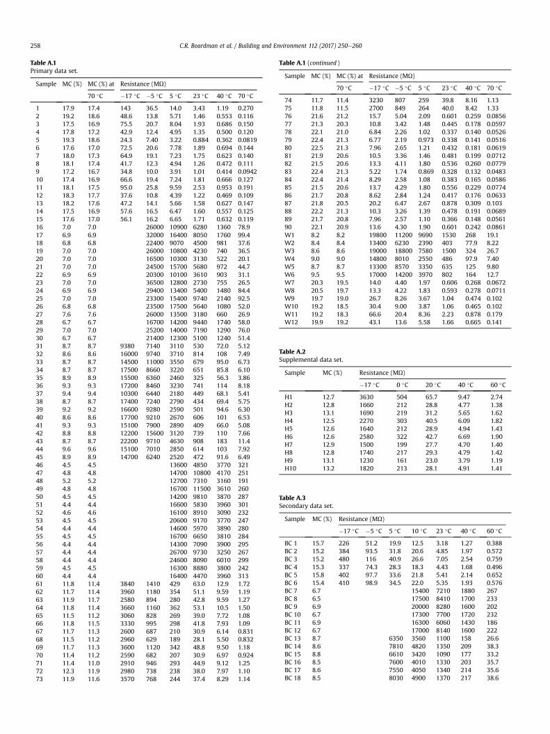
Table A.1Primary data set.

Sample MC (%) MC (%) at Resistance (MU)

70 �C �17 �C �5 �C 5 �C 23 �C 40 �C 70 �C

1 17.9 17.4 143 36.5 14.0 3.43 1.19 0.2702 19.2 18.6 48.6 13.8 5.71 1.46 0.553 0.1163 17.5 16.9 75.5 20.7 8.04 1.93 0.686 0.1504 17.8 17.2 42.9 12.4 4.95 1.35 0.500 0.1205 19.3 18.6 24.3 7.40 3.22 0.884 0.362 0.08196 17.6 17.0 72.5 20.6 7.78 1.89 0.694 0.1447 18.0 17.3 64.9 19.1 7.23 1.75 0.623 0.1408 18.1 17.4 41.7 12.3 4.94 1.26 0.472 0.1119 17.2 16.7 34.8 10.0 3.91 1.01 0.414 0.094210 17.4 16.9 66.6 19.4 7.24 1.81 0.666 0.12711 18.1 17.5 95.0 25.8 9.59 2.53 0.953 0.19112 18.3 17.7 37.6 10.8 4.39 1.22 0.469 0.10913 18.2 17.6 47.2 14.1 5.66 1.58 0.627 0.14714 17.5 16.9 57.6 16.5 6.47 1.60 0.557 0.12515 17.6 17.0 56.1 16.2 6.65 1.71 0.632 0.11916 7.0 7.0 26000 10900 6280 1360 78.917 6.9 6.9 32000 16400 8050 1760 99.418 6.8 6.8 22400 9070 4500 981 37.619 7.0 7.0 26000 10800 4230 740 36.520 7.0 7.0 16500 10300 3130 522 20.121 7.0 7.0 24500 15700 5680 972 44.722 6.9 6.9 20300 10100 3610 903 31.123 7.0 7.0 36500 12800 2730 755 26.524 6.9 6.9 29400 13400 5400 1480 84.425 7.0 7.0 23300 15400 9740 2140 92.526 6.8 6.8 23500 17500 5640 1080 52.027 7.6 7.6 26000 13500 3180 660 26.928 6.7 6.7 16700 14200 9440 1740 58.029 7.0 7.0 25200 14000 7190 1290 76.030 6.7 6.7 21400 12300 5100 1240 51.431 8.7 8.7 9380 7140 3110 530 72.0 5.1232 8.6 8.6 16000 9740 3710 814 108 7.4933 8.7 8.7 14500 11000 3550 679 95.0 6.7334 8.7 8.7 17500 8660 3220 651 85.8 6.1035 8.9 8.9 15500 6360 2460 325 56.3 3.8636 9.3 9.3 17200 8460 3230 741 114 8.1837 9.4 9.4 10300 6440 2180 449 68.1 5.4138 8.7 8.7 17400 7240 2790 434 69.4 5.7539 9.2 9.2 16600 9280 2590 501 94.6 6.3040 8.6 8.6 17700 9210 2670 606 101 6.5341 9.3 9.3 15100 7900 2890 409 66.0 5.0842 8.8 8.8 12200 15600 3120 739 110 7.6643 8.7 8.7 22200 9710 4630 908 183 11.444 9.6 9.6 15100 7010 2850 614 103 7.9245 8.9 8.9 14700 6240 2520 472 91.6 6.4946 4.5 4.5 13600 4850 3770 32147 4.8 4.8 14700 10800 4170 25148 5.2 5.2 12700 7310 3160 19149 4.8 4.8 16700 11500 3610 26050 4.5 4.5 14200 9810 3870 28751 4.4 4.4 16600 5830 3960 30152 4.6 4.6 16100 8910 3090 23253 4.5 4.5 20600 9170 3770 24754 4.4 4.4 14600 5970 3890 28055 4.5 4.5 16700 6650 3810 28456 4.4 4.4 14300 7090 3900 29557 4.4 4.4 26700 9730 3250 26758 4.4 4.4 24600 8090 6010 29959 4.5 4.5 16300 8880 3800 24260 4.4 4.4 16400 4470 3960 31361 11.8 11.4 3840 1410 429 63.0 12.9 1.7262 11.7 11.4 3960 1180 354 51.1 9.59 1.1963 11.9 11.7 2580 894 280 42.8 9.59 1.2764 11.8 11.4 3660 1160 362 53.1 10.5 1.5065 11.5 11.2 3060 828 269 39.0 7.72 1.0866 11.8 11.5 3330 995 298 41.8 7.93 1.0967 11.7 11.3 2600 687 210 30.9 6.14 0.83168 11.5 11.2 2960 629 189 28.1 5.50 0.83269 11.7 11.3 3600 1120 342 48.8 9.50 1.1870 11.4 11.2 2590 682 207 30.9 6.97 0.92471 11.4 11.0 2910 946 293 44.9 9.12 1.2572 12.3 11.9 2980 738 238 38.0 7.97 1.1073 11.9 11.6 3570 768 244 37.4 8.29 1.14

Table A.2Supplemental data set.

Sample MC (%) Resistance (MU)

�17 �C 0 �C 20 �C 40 �C 60 �C

H1 12.7 3630 504 65.7 9.47 2.74H2 12.8 1660 212 28.8 4.77 1.38H3 13.1 1690 219 31.2 5.65 1.62H4 12.5 2270 303 40.5 6.09 1.82H5 12.6 1640 212 28.9 4.94 1.43H6 12.6 2580 322 42.7 6.69 1.90H7 12.9 1500 199 27.7 4.70 1.40H8 12.8 1740 217 29.3 4.79 1.42H9 13.1 1230 161 23.0 3.79 1.19H10 13.2 1820 213 28.1 4.91 1.41

Table A.1 (continued )

Sample MC (%) MC (%) at Resistance (MU)

70 �C �17 �C �5 �C 5 �C 23 �C 40 �C 70 �C

74 11.7 11.4 3230 807 259 39.8 8.16 1.1375 11.8 11.5 2700 849 264 40.0 8.42 1.3376 21.6 21.2 15.7 5.04 2.09 0.601 0.259 0.085677 21.3 20.3 10.8 3.42 1.48 0.445 0.178 0.059778 22.1 21.0 6.84 2.26 1.02 0.337 0.140 0.052679 22.4 21.3 6.77 2.19 0.973 0.338 0.141 0.051680 22.5 21.3 7.96 2.65 1.21 0.432 0.181 0.061981 21.9 20.6 10.5 3.36 1.46 0.481 0.199 0.071282 21.5 20.6 13.3 4.11 1.80 0.536 0.260 0.077983 22.4 21.3 5.22 1.74 0.869 0.328 0.132 0.048384 22.4 21.4 8.29 2.58 1.08 0.383 0.165 0.058685 21.5 20.6 13.7 4.29 1.80 0.556 0.229 0.077486 21.7 20.8 8.62 2.84 1.24 0.417 0.176 0.063387 21.8 20.5 20.2 6.47 2.67 0.878 0.309 0.10388 22.2 21.3 10.3 3.26 1.39 0.478 0.191 0.068989 21.7 20.8 7.96 2.57 1.10 0.366 0.148 0.056190 22.1 20.9 13.6 4.30 1.90 0.601 0.242 0.0861W1 8.2 8.2 19800 11200 9690 1530 268 19.1W2 8.4 8.4 13400 6230 2390 403 77.9 8.22W3 8.6 8.6 19000 18800 7580 1500 324 26.7W4 9.0 9.0 14800 8010 2550 486 97.9 7.40W5 8.7 8.7 13300 8570 3350 635 125 9.80W6 9.5 9.5 17000 14200 3970 802 164 12.7W7 20.3 19.5 14.0 4.40 1.97 0.606 0.268 0.0672W8 20.5 19.7 13.3 4.22 1.83 0.593 0.278 0.0711W9 19.7 19.0 26.7 8.26 3.67 1.04 0.474 0.102W10 19.2 18.5 30.4 9.00 3.87 1.06 0.465 0.102W11 19.2 18.3 66.6 20.4 8.36 2.23 0.878 0.179W12 19.9 19.2 43.1 13.6 5.58 1.66 0.665 0.141

Table A.3Secondary data set.

Sample MC (%) Resistance (MU)

�17 �C �5 �C 5 �C 10 �C 23 �C 40 �C 60 �C

BC 1 15.7 226 51.2 19.9 12.5 3.18 1.27 0.388BC 2 15.2 384 93.5 31.8 20.6 4.85 1.97 0.572BC 3 15.2 480 116 40.9 26.6 7.05 2.54 0.759BC 4 15.3 337 74.3 28.3 18.3 4.43 1.68 0.496BC 5 15.8 402 97.7 33.6 21.8 5.41 2.14 0.652BC 6 15.4 410 98.9 34.5 22.0 5.35 1.93 0.576BC 7 6.7 15400 7210 1880 267BC 8 6.5 17500 8410 1700 233BC 9 6.9 20000 8280 1600 202BC 10 6.7 17300 7700 1720 232BC 11 6.9 16300 6060 1430 186BC 12 6.7 17000 8140 1600 222BC 13 8.7 6350 3560 1100 158 26.6BC 14 8.6 7810 4820 1350 209 38.3BC 15 8.8 6610 3420 1090 177 33.2BC 16 8.5 7600 4010 1330 203 35.7BC 17 8.6 7550 4050 1340 214 35.6BC 18 8.5 8030 4900 1370 217 38.6

C.R. Boardman et al. / Building and Environment 112 (2017) 250e260258

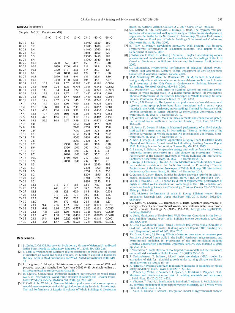
Table A.3 (continued )

Sample MC (%) Resistance (MU)

�17 �C �5 �C 5 �C 10 �C 23 �C 40 �C 60 �C

BC 19 5.3 13400 3380 560BC 20 5.2 11700 3400 579BC 21 5.4 11400 2760 441BC 22 5.3 9080 3660 620BC 23 5.3 13000 3450 562BC 24 5.4 13200 2940 493BC 25 10.8 2660 852 487 153 29.3 6.18BC 26 10.6 3650 1200 665 218 38.8 8.08BC 27 10.5 2320 717 398 114 23.7 4.51BC 28 10.6 3120 1030 570 177 33.7 6.96BC 29 10.8 2590 788 440 136 25.6 5.39BC 30 10.8 3380 1100 608 194 35.4 7.77BC 31 21.5 10.1 3.28 1.52 0.999 0.423 0.181 0.0894BC 32 21.4 6.68 2.24 1.05 0.736 0.305 0.143 0.0682BC 33 21.3 11.9 3.84 1.74 1.22 0.487 0.221 0.0983BC 34 21.3 12.8 3.98 1.77 1.17 0.457 0.214 0.101BC 35 21.4 9.63 3.32 1.47 0.982 0.420 0.188 0.0954BC 36 21.5 14.4 4.52 2.05 1.45 0.556 0.247 0.112TX 1 17.1 143 32.3 12.0 7.60 1.92 0.826 0.256TX 2 17.6 126 30.0 11.6 7.34 2.06 0.852 0.281TX 3 18.5 46.7 12.6 4.99 3.21 1.03 0.410 0.142TX 4 18.1 107 26.0 10.0 6.35 2.02 0.745 0.251TX 5 18.1 47.6 12.6 4.91 3.17 0.96 0.402 0.139TX 6 18.1 55.5 14.5 5.67 3.59 1.12 0.471 0.161TX 7 8.0 5850 1670 257 26.9TX 8 8.0 7700 2250 353 35.8TX 9 7.9 7750 2210 323 28.9TX 10 8.1 6350 1530 244 24.2TX 11 7.8 9500 2630 405 36.4TX 12 7.6 8700 2420 377 30.7TX 13 9.7 2300 1160 269 36.8 6.78TX 14 9.6 2350 1200 262 34.1 6.05TX 15 9.7 2090 1090 247 33.6 6.1TX 16 9.7 2080 1060 246 35.7 6.6TX 17 10.0 1780 939 212 30.1 5.6TX 18 9.9 2050 1040 232 31.1 5.6TX 19 6.3 8940 2080 304TX 20 6.3 7330 1960 284TX 21 6.5 8260 1810 230TX 22 6.2 8270 1950 274TX 23 6.2 8740 1920 254TX 24 6.2 9480 2250 318TX 25 12.1 715 214 118 32.6 7.67 1.69TX 26 12.1 749 218 122 36.2 7.69 1.66TX 27 12.2 441 123 60.0 18.8 4.24 0.931TX 28 12.1 818 240 131 39.6 8.31 1.85TX 29 12.2 537 153 76.2 25.3 5.24 1.14TX 30 12.0 604 172 95.8 24.5 5.48 1.23TX 31 23.1 9.43 2.96 1.32 1.02 0.409 0.171 0.0751TX 32 23.2 6.91 2.16 0.974 0.757 0.302 0.131 0.0583TX 33 23.3 7.38 2.38 1.10 0.881 0.348 0.150 0.0689TX 34 23.3 4.28 1.38 0.637 0.491 0.209 0.0879 0.0418TX 35 23.1 5.84 1.86 0.922 0.687 0.294 0.119 0.060TX 36 23.1 4.64 1.47 0.699 0.528 0.229 0.0983 0.0466

C.R. Boardman et al. / Building and Environment 112 (2017) 250e260 259

References

[1] J.I. Zerbe, Z. Cai, G.B. Harpole, An Evolutionary History of Oriented Strandboard(OSB), Forest Products Laboratory, Madison, WI., 2015. FPL-GTR-236.

[2] C. Carll, A. Wiedenhoeft, Moisture-related properties of wood and the effectsof moisture on wood and wood products, in: Moisture Control in Buildings:the Key Factor in Mold Preventions, second ed., ASTM International, 2009. MNL18.

[3] L. Haughton, C. Murphy, “Moisture exchange”: performance of OSB andplywood structural panels, Interface (June 2003) 6e13. Available online at,http://suncrestshed.com/Plywood-OSB.pdf.

[4] D. Cautley, Comparative measured moisture performance of wood-framewalls, in: Proceedings, Wood-frame Housing Durability and Disaster Issues,Forest Products Society, Madison, WI, 2004, pp. 201e209.

[5] C. Carll, A. TenWolde, R. Munson, Moisture performance of a contemporarywood-frame house operated at design indoor humidity levels, in: Proceedings,Thermal Performance of Exterior Envelopes of Whole Buildings X, Clearwater

Beach, FL, ASHRAE, Atlanta, GA, Dec. 2-7, 2007. ORNL 07-Go1409/aas.[6] S.D. Gatland II, A.N. Karagiozis, C. Murray, K. Ueno, The hygrothermal per-

formance of wood-framed wall systems using a relative humidity-dependentvapor retarder in the Pacific Northwest, in: Proceedings, Thermal Performanceof the Exterior Envelopes of Whole Buildings X International Conference,Clearwater Beach, FL, USA, 2007.

[7] R. Tichy, C. Murray, Developing Innovative Wall Systems that ImproveHygrothermal Performance of Residential Buildings, Final Report to U.S.Department of Energy, 2007.

[8] J. Wilkinson, K. Ueno, D. De Rose, J.F. Straube, D. Fugler, Understanding vapourpermeance and condensation in wall assemblies, in: Proceedings of the 11thCanadian Conference on Building Science and Technology, Banff, Alberta,2007.

[9] C.J. Schumacher, Hygrothermal Performance of Insulated, Sloped, Wood-Framed Roof Assemblies, Master’s Thesis, Department of Civil Engineering,University of Waterloo, Ontario, Canada, 2008.

[10] M.M. Armstrong, W. Maref, M. Rousseau, W. Lei, M. Nicholls, A field moni-toring study of interstitial condensation in wood-frame walls in cold climate,in: Proceedings of the 12th Canadian Conference on Building Science andTechnology, Montr�eal, Quebec, May 6-8, 2009.

[11] S.C. Drumheller, C.G. Carll, Effect of cladding systems on moisture perfor-mance of wood-framed walls in a mixed-humid climate, in: Proceedings,Thermal Performance of the Exterior Envelopes of Whole Buildings XI Inter-national Conference, Clearwater Beach, FL, USA, 2010.

[12] S. Yuan, A.N. Karagiozis, The hygrothermal performance of wood-framed wallsystems using spray polyurethane foam insulations and a smart vaporretarder in the Pacific Northwest, in: Proceedings, Thermal Performance of theExterior Envelopes of Whole Buildings XI International Conference, Clear-water Beach, FL, USA, 5e9 December 2010.

[13] T.A. Weston, L.C. Minnich, Moisture measurements and condensation poten-tial in wood frame walls in a hot-humid climate, J. Test. Eval. 39 (2011)395e409.

[14] L.B. Arena, D. Owens, P. Mantha, Measured performance of an R-40 double-stud wall in climate zone 5a, in: Proceedings, Thermal Performance of theExterior Envelopes of Whole Buildings XII International Conference, Clear-water Beach, FL, USA, 1e5 December 2013.

[15] A. Grin, J. Smegal, J. Lstiburek, Application of Spray Foam Insulation underPlywood and Oriented Strand Board Roof Sheathing, Building America Report1312, Building Science Corporation, Somerville, MA, USA, 2013.

[16] G. Parsons, B. Lieburn, Comparative energy and wall performance of twelveresidential houses constructed in a cold climate, in: Proceedings, ThermalPerformance of the Exterior Envelopes of Whole Buildings XII InternationalConference, Clearwater Beach, FL, USA, 1e5 December 2013.

[17] J. Smegal, J. Lstiburek, J. Straube, A. Grin, Moisture-related durability of wallswith exterior insulation in the Pacific Northwest, in: Proceedings, ThermalPerformance of the Exterior Envelopes of Whole Buildings XII InternationalConference, Clearwater Beach, FL, USA, 1e5 December 2013.

[18] C. Craven, R. Garber-Slaght, Exterior insulation envelope retrofits in cold cli-mates: implications for moisture control, HVAC R Res. 20 (2014) 384e394.

[19] M. Fox, J. Straube, H. Ge, T. Trainor, Field test of hygrothermal performance ofhighly insulated wall assemblies, in: Proceedings of the 14th Canadian Con-ference on Building Science and Technology, Toronto, Canada, 28e30 October2014, pp. 101e110.

[20] HIRL, Moisture Performance of Walls in Energy Efficient Homes, HomeInnovation Research Labs, Upper Marlboro, MD, 2014. Report 5932.001_08142014.

[21] S.V. Glass, V. Kochkin, S.C. Drumheller, L. Barta, Moisture performance ofenergy eefficient and conventional wood-frame wall assemblies in a mixed-humid climate, Buildings 5 (2015) 759e782, http://dx.doi.org/10.3390/buildings5030759.

[22] K. Ueno, Monitoring of Double-Stud Wall Moisture Conditions in the North-east, Building America Report 1501, Building Science Corporation, Westford,MA, USA, 2015.

[23] K. Ueno, J.W. Lstiburek, Field Testing Unvented Roofs with Asphalt Shingles inCold and Hot-Humid Climates, Building America Report 1409, Building Sci-ence Corporation, Westford, MA, USA, 2015.

[24] S.V. Glass, B. Yeh, B.J. Herzog, Effects of exterior insulation on moisture per-formance of wood-frame walls in the Pacific Northwest: measurements andhygrothermal modeling, in: Proceedings of the 3rd Residential BuildingDesign & Construction Conference, University Park, PA, USA, March 2-3, 2016,pp. 292e311.

[25] E. Vereecken, S. Roels, Review of mould prediction models and their influenceon mould risk evaluation, Build. Environ. 51 (2012) 296e310.

[26] S. Thelandersson, T. Isaksson, Mould resistance design (MRD) model forevaluation of risk for microbial growth under varying climate conditions,Build. Environ. 65 (2013) 18e25.

[27] K. Pietrzyk, A systemic approach to moisture problems in buildings for mouldsafety modelling, Build. Environ. 86 (2015) 50e60.

[28] H. Viitanen, J. Vinha, K. Salminen, T. Ojanen, R. Peuhkuri, L. Paajanen, et al.,Moisture and bio-deterioration risk of building materials and structures,J. Build. Phys. 33 (2010) 201e224.

[29] H. Viitanen, T. Toratti, L. Makkonen, R. Peuhkuri, T. Ojanen, L. Ruokolainen, etal., Towards modelling of decay risk of wooden materials, Eur. J. Wood WoodProd. 68 (2010) 303e313.

[30] H. Saito, K. Fukuda, T. Sawachi, Integration model of hygrothermal analysis

C.R. Boardman et al. / Building and Environment 112 (2017) 250e260260

with decay process for durability assessment of building envelopes, Build.Simul. 5 (2012) 315e324.

[31] T. Isaksson, C. Brischke, S. Thelandersson, Development of decay performancemodels for outdoor timber structures, Mater. Struct. 46 (2013) 1209e1225.

[32] C. Brischke, L. Meyer-Veltrup, Modelling timber decay caused by brown rotfungi, Mater. Struct. 49 (2016) 3281e3291.

[33] S.L. Zelinka, D. Derome, S.V. Glass, Combining hygrothermal and corrosionmodels to predict corrosion of metal fasteners embedded in wood, Build.Environ. 46 (2011) 2060e2068.

[34] S.L. Zelinka, S.V. Glass, D. Derome, The effect of moisture content on thecorrosion of fasteners embedded in wood subjected to alkaline copper qua-ternary treatment, Corros. Sci. 83 (2014) 67e74.

[35] S.L. Zelinka, S.V. Glass, C.R. Boardman, D. Derome, Comparison of the corrosionof fasteners embedded in wood measured in outdoor exposure with thepredictions from a combined hygrothermal-corrosion model, Corros. Sci. 102(2016) 178e185.

[36] P.I. Morris, Understanding Biodeterioration of Wood in Structures, ForinteckCanada Corp., British Columbia Building Envelope Council. http://cwc.ca/wp-content/uploads/aboutdecay-biodeterioration.pdf (Accessed 15 November2016).

[37] C.A. Clausen, Wood Handbook, Ch. 14: Biodeterioration of Wood, ForestProducts Laboratory, Madison, WI, 2010. FPL-GTR-190, http://www.fpl.fs.fed.us/documnts/fplgtr/fplgtr190/chapter_14.pdf (Accessed 15 November 2016).

[38] C.G. Carll, T.L. Highley, Decay of wood and wood-based products aboveground in buildings, J. Test. Eval. 27 (2) (1999) 150e158.

[39] L. Arena, P. Mantha, Moisture Research e Optimizing Wall Assemblies, USDOE, Building Technologies Program, 2013, http://dx.doi.org/10.2172/1079731. Report DOE/GO-102013e3813.

[40] S.M. Cornick, W. Maref, F. Tariku, Verification and Validation: EstablishingConfidence in Hygrothermal Tools, National Research Council of Canada,2009. Research Report IRC-RR-278.

[41] A. Karagiozis, Application of advanced tools to develop energy efficientbuilding envelopes that are durable, in: Proceedings, Performance of ExteriorEnvelopes of Whole Buildings IX International Conference, Clearwater Beach,FL, USA, 5e10 December 2004.

[42] G. Finch, J. Straube, Ventilated wall claddings: review, field performance, andhygrothermal modeling, in: Proceedings, Thermal Performance of the ExteriorEnvelopes of Whole Buildings X International Conference, Clearwater Beach,FL, USA, 2e7 December 2007.

[43] F. Tariku, S.M. Cornick, M.A. Lacasse, Simulation of wind-driven rain pene-tration effects on the performance of a stucco-clad wall, in: Proceedings,Thermal Performance of the Exterior Envelopes of Whole Buildings X Inter-national Conference, Clearwater Beach, FL, USA, 2007.

[44] J. Straube, J. Smegal, Building America Special Research Project: High-r WallsCase Study Analysis, Research Report BA-0903, Building Science Corporation,Somerville, MA, USA, 2009.

[45] M. Pazera, M. Salonvaara, Drying characteristics of spray-applied cellulosefiber insulation, J. Test. Eval. 39 (2011) 219e229.

[46] S. Pallin, M. Kehrer, W.A. Miller, A hygrothermal risk analysis applied toresidential unvented attics, in: Proceedings, Thermal Performance of theExterior Envelopes of Whole Buildings XII International Conference, Clear-water Beach, FL, USA, 1e5 December 2013.

[47] M. Salonvaara, A. Karagiozis, A. Desjarlais, Moisture performance of sealedattics in climate zones 1 to 4, in: Proceedings, Thermal Performance of theExterior Envelopes of Whole Buildings XII International Conference, Clear-water Beach, FL, USA, 1e5 December 2013.

[48] H.H. Saber, W. Maref, Risk of condensation and mould growth in wood-framewall systems with different exterior insulations, in: Proceedings of BuildingEnclosure Science & Technology Conf. (BEST4), April 12-15, 2015 (Kansas City,Missouri, USA).

[49] S.V. Glass, A. TenWolde, Review of In-service Moisture and TemperatureConditions in Wood-frame Buildings, Forest Products Laboratory, Madison,WI, 2007. FPL-GTR-174.

[50] J. Langmans, R. Klein, S. Roels, Hygrothermal risks of using exterior air barriersystems for highly insulated light weight walls: a laboratory investigation,Build. Environ. 56 (2012) 192e202.

[51] D.M. Onysko, C. Schumacher, P. Garrahan, Field measurements of moisture inbuilding materials and assemblies: pitfalls and error assessment, in: Pro-ceedings of BEST 1 Conference, June 10-12, 2008 (Minneapolis, MN).

[52] J. Straube, D. Onysko, C. Schumacher, Methodology and design of field ex-periments for monitoring hygrothermal performance of wood frame enclo-sures, J. Therm. Env. Buid. Sci. 26 (2) (2002) 123e151, http://dx.doi.org/

10.1106/109719602028098.[53] W.L. James, Electric Moisture Meters for Wood, Forest Products Laboratory,

Madison, WI., 1963. FPL-08.[54] W.L. James, Electric Moisture Meters for Wood, Forest Products Laboratory,

Madison, WI., 1988. FPL-GTR-6.[55] F. Pfaff, P. Garrahan, New temperature correction factors for the portable

resistance-type moisture meter, For. Prod. J. 36 (3) (1986) 28e30.[56] P. Garrahan, Moisture meter correction factors, in: Proceeds of a Seminar on

In-Grade Testing of Structural Lumber, Madison, WI,, Forest Products Labo-ratory, US Forest Service, Madison WI, April 25-26, 1988.

[57] W. James, Effect of temperature on readings of electric moisture meters, For.Prod. J. 18 (10) (1968) 23e31.

[58] C.R. Boardman, S.V. Glass, C.G. Carll, Moisture meter calibrations for untreatedand ACQ-treated southern yellow pine lumber and plywood, J. Test. Eval. 40(1) (2012) JTE103895.

[59] W. Maref, M.A. Lacasse, D. Booth, Experimental assessment of hygrothermalproperties of wood-frame wall assemblies e moisture content calibrationcurve for OSB using moisture pins, J. ASTM Int. 7 (1) (2010), http://dx.doi.org/10.1520/JAI102091.

[60] S. Zelinka, S.V. Glass, D.S. Stone, A percolation model for electrical conductionin wood with implications for wood-water relations, Wood Fiber Sci. 40 (4)(2008) 544e552.

[61] R.E. Hummel, Electrical Properties of Polymers, Ceramics, Dielectrics, andAmorphous Materials, Ch. 9 in Electronic Properties of Materials, Springer-Verlag, 2001.

[62] S. Aziz, Z.G.Z. Abidin, Electrical conduction mechanism in solid polymerelectrolytes: new concepts to Arrhenius equation, J. Soft Matter (2013), http://dx.doi.org/10.1155/2013/323868.

[63] S.D. Kasap, Principles of Electronic Materials and Devices (Chapter 2). Elec-trical and Thermal Conduction in Solids, third ed., McGraw-Hill, 2015.

[64] ASTM D4442. Standard Test Methods for Direct Moisture Content Measure-ment of Wood and Wood-Based Materials, American Standard for Testing andMaterials, West Conshohocken, PA, 2015.

[65] SAS. Cary, NC: SAS Institute, Inc., 2013. http://support.sas.com/documentation/94/. (November 16, 2016).

[66] R Core Team, R: A Language and Environment for Statistical Computing. RFoundation for Statistical Computing, 2016. Vienna, Austria, https://www.R-project.org/.

[67] S.C. Zylkowski, Dimensional Stability of Structural-Use Panels, Report No.R&D86L-43, American Plywood Association, Tacoma, WA, 1986.

[68] R.F. Richards, D.M. Burch, W.C. Thomas, Water vapor sorption measurementsof common building materials, ASHRAE Trans. 98 (1992) 475e483.

[69] N. Sekino, A. Suematsu, H. Kohrai, E. Yasui, Measurements of sorption iso-therms of selected commercial wood-based panels and predictions of mois-ture content changes in service, Mokuzai Gakkaishi 45 (1999) 237e243.

[70] Q.L. Wu, Y.K. Ren, Characterization of sorption behavior of oriented strand-board under long-term cyclic humidity exposure condition, Wood Fiber Sci.32 (2000) 404e418.

[71] M.K. Kumaran, J.C. Lackey, N. Normandin, F. Tariku, D. van Reenen, A Thermaland Moisture Transport Property Database for Common Building and Insu-lating Materials: Final Report from ASHRAE Research Project 1018-RP,American Society of Heating, Refrigerating and Air-Conditioning Engineers,Inc., Atlanta, GA, 2002.

[72] M.K. Kumaran, J.C. Lackey, N. Normandin, F. Tariku, D. Van Reenen, Variationsin the hygrothermal properties of several wood-based building products, in:J. Carmeliet, H. Hens, G. Vermeir (Eds.), Research in Building Physics: Pro-ceedings of the 2nd International Conference on Building Physics, Swets &Zeitlinger B.V., Antwerpen, Belgium, 2003, pp. 35e42.

[73] A. Karagiozis, K. Wilkes, Hygrothermal Properties of Selected Materials.Report 2, ASHRAE Research Project 1091, Development of Design Strategiesfor Rainscreen and Sheathing Membrane Performance in Wood Frame Walls,American Society of Heating, Refrigerating and Air-Conditioning Engineers,Inc., Atlanta, GA, USA, 2004.

[74] T. Ojanen, J. Ahonen, C.J. Simonson, Moisture performance characteristics ofOSB and spruce plywood exterior sheathing products, in: P. Fazio, H. Ge, J. Rao,G. Desmarais (Eds.), Research in Building Physics and Building Engineering:Proceedings of the Third International Building Physics Conference, Taylor &Francis, Montreal, Canada, 2006, pp. 97e105.

[75] I.D. Hartley, S.Q. Wang, Y. Zhang, Water vapor sorption isotherm modeling ofcommercial oriented strand panel based on species groups and resin type,Build. Environ. 42 (2007) 3655e3659.