Simple Linear Regression

1

1. Introduction

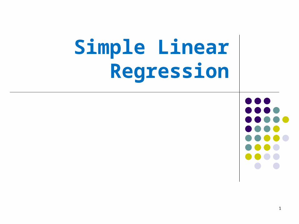
Response (out come or dependent) variable (Y): height of the wifePredictor (explanatory or independent) variable (X): height of the husband

Example:

George Bush :1.81mLaura Bush: ?

David Beckham: 1.83mVictoria Beckham: 1.68m

Brad Pitt: 1.83mAngelina Jolie: 1.70m

● To predict height of the wife in a couple, based on the husband’s height

2

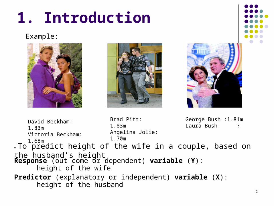
Regression analysis:

● The earliest form of linear regression was the method of least squares, which was published by Legendre in 1805, and by Gauss in 1809.

● The method was extended by Francis Galton in the 19th century to describe a biological phenomenon.

● This work was extended by Karl Pearson and Udny Yule to a more general statistical context around 20th century.

●　 regression analysis is a statistical methodology to estimate the relationship of a response variable to a set of predictor variable.

History:

● 　 when there is just one predictor variable, we will use simple linear regression. When there are two or more predictor variables, we use multiple linear regression.

● when it is not clear which variable represents a response and which is a predictor, correlation analysis is used to study the strength of the relationship

3

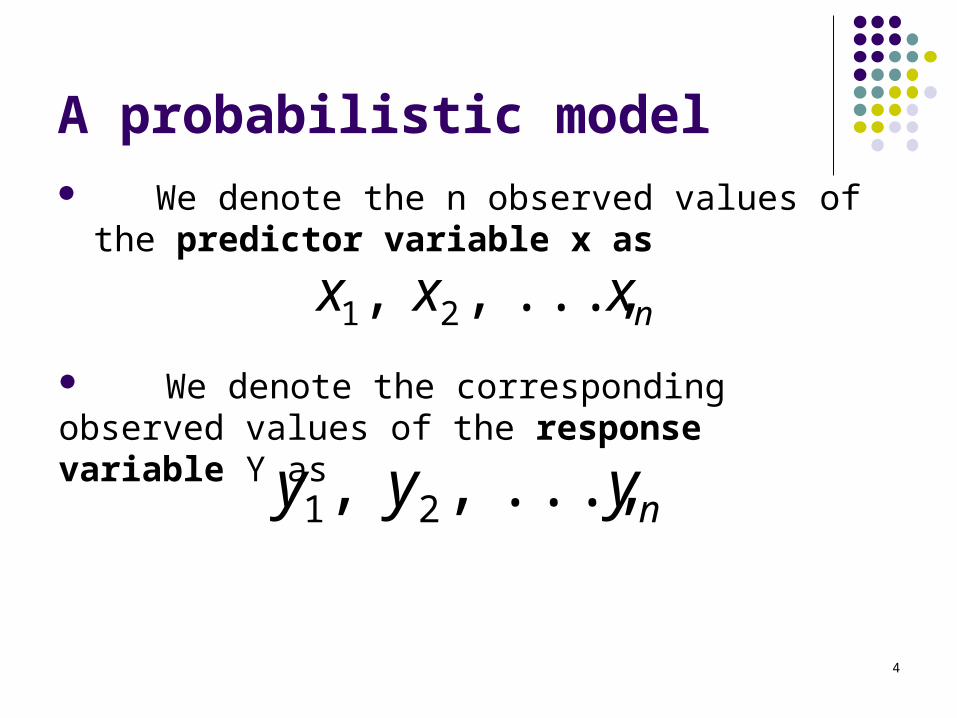
A probabilistic model We denote the n observed values of the

predictor variable x as

nxxx ...,,, 21

We denote the corresponding observed values of the response variable Y as

nyyy ...,,, 21

4

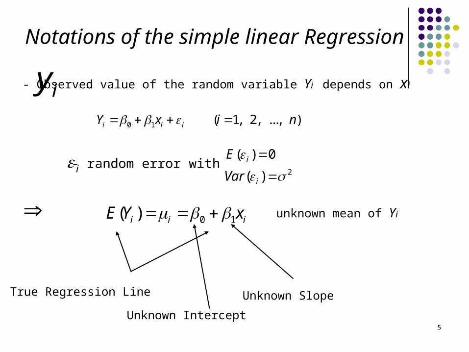
Notations of the simple linear Regression

- Observed value of the random variable Yi depends on xi iy0 1 ( 1, 2, ..., )i i iY x i n

i 2)(

0)(

i

i

Var

E

0 1( )i i iE Y x

- random error with

unknown mean of Yi

Unknown SlopeTrue Regression Line

Unknown Intercept5

6

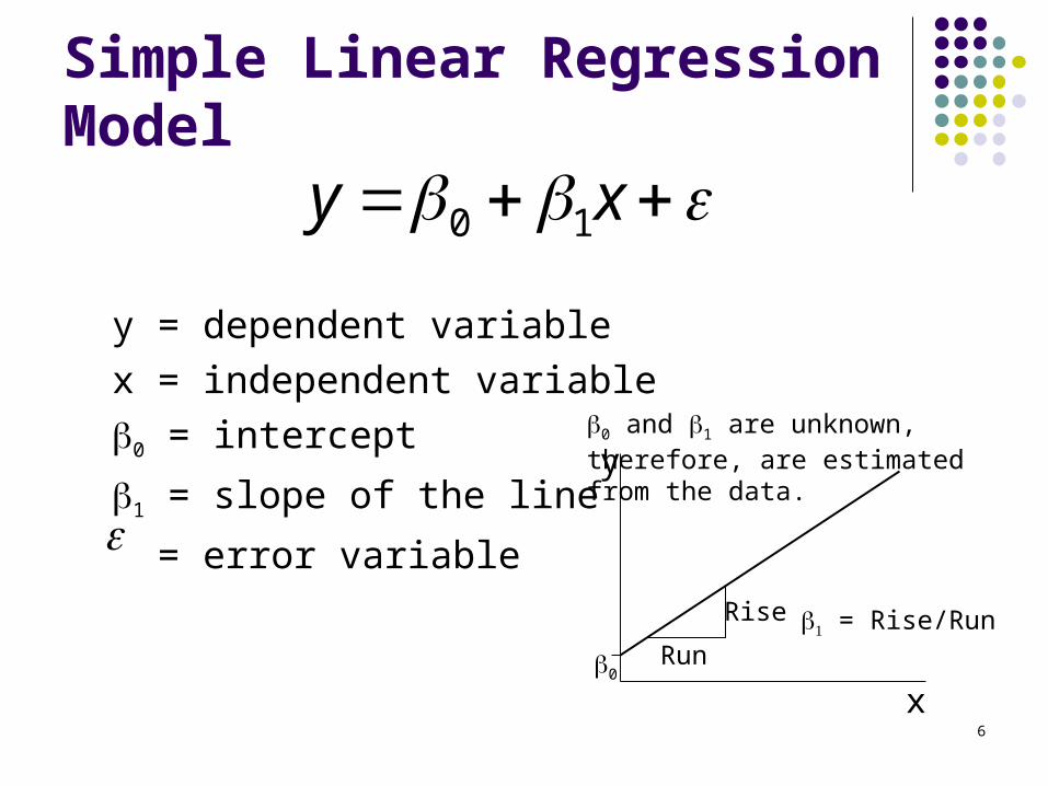
Simple Linear Regression Model

y = dependent variable

x = independent variable

0 = intercept

1 = slope of the line

= error variable

x

y

0Run

Rise = Rise/Run

0 and 1 are unknown,therefore, are estimated from the data.

xy 10

7

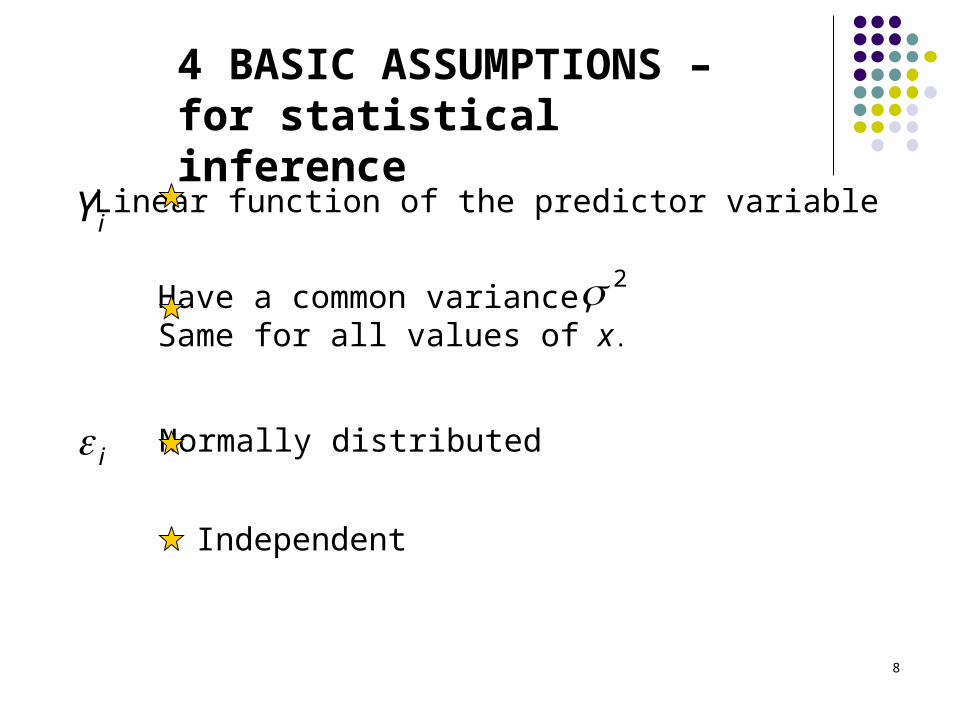
iY

2

Linear function of the predictor variable

Have a common variance,Same for all values of x.

i Normally distributed

4 BASIC ASSUMPTIONS – for statistical inference

Independent

8

Comments:1. Linear not in x

But in the parameters and

2. Predictor variable is not set as predetermined fixed values, is random along with Y. The model can be considered as a conditional model

xYE log)( 10

10

Example:

xxXYE 10)|(

linear, logx = x*

Example: Height and Weight of the children.Height (X) – given Weight (Y) – predict

Conditional expectation of Y given X = x

9

2. Fitting the Simple Linear Regression

Model

2.1 Least Squares (LS) Fit

10

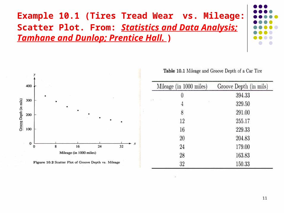
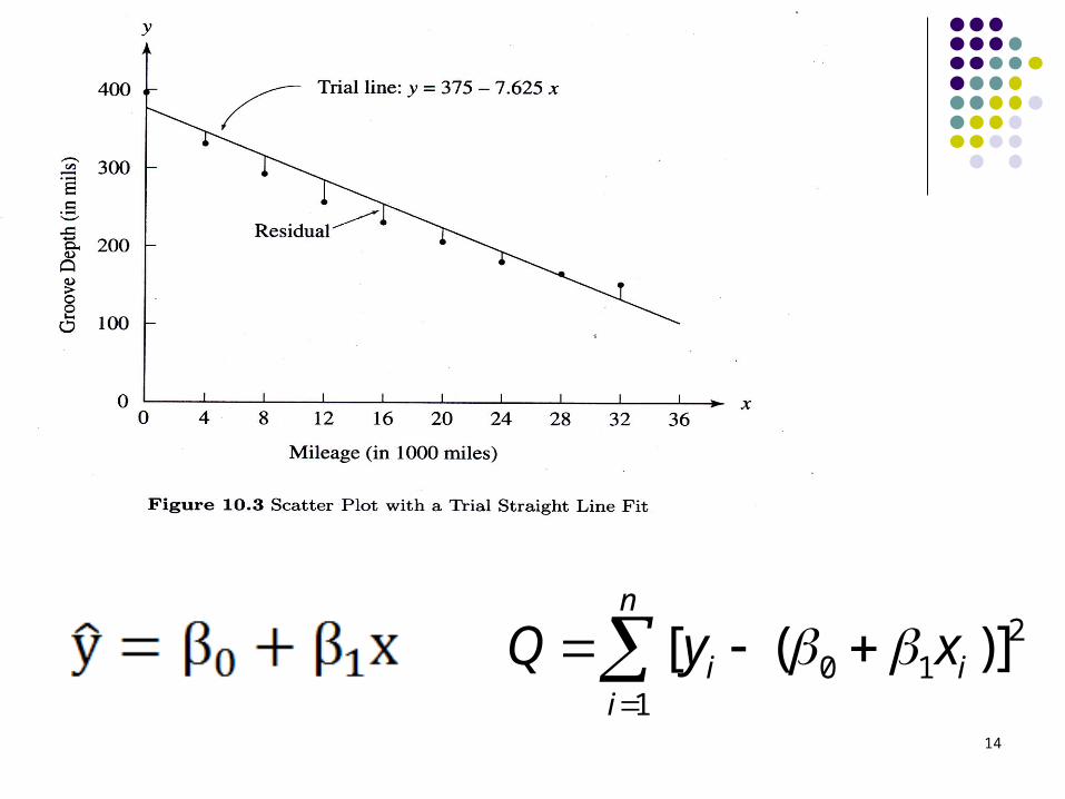
Example 10.1 (Tires Tread Wear vs. Mileage: Scatter Plot. From: Statistics and Data Analysis; Tamhane and Dunlop; Prentice Hall. )

11

12

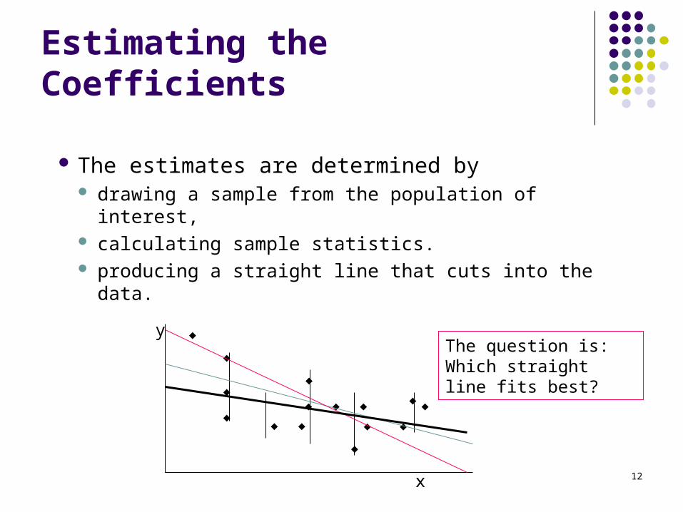
Estimating the Coefficients

The estimates are determined by drawing a sample from the population of interest, calculating sample statistics. producing a straight line that cuts into the data.

The question is:Which straight line fits best?

x

y

133

3

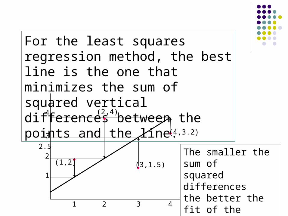
For the least squares regression method, the best line is the one that minimizes the sum of squared vertical differences between the points and the line.

41

1

4

(1,2)

2

2

(2,4)

(3,1.5)

(4,3.2)

2.5The smaller the sum of squared differencesthe better the fit of the line to the data.

20 1

1

[ ( )]n

i ii

Q y x

14

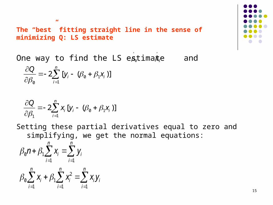
The “best” fitting straight line in the sense of minimizing Q: LS estimate

One way to find the LS estimate and

Setting these partial derivatives equal to zero and simplifying, we get the normal equations:

1

0 11 1

20 1

1 1 1

n n

i ii i

n n n

i i i ii i i

n x y

x x x y

0 110

0 111

2 [ ( )]

2 [ ( )]

n

i ii

n

i i ii

Qy x

Qx y x

0

15

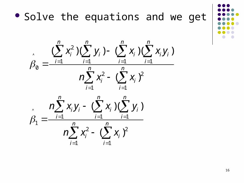
Solve the equations and we get

2

1 1 1 10

2 2

1 1

1 1 11

2 2

1 1

( )( ) ( )( )

( )

( )( )

( )

n n n n

i i i i ii i i i

n n

i ii i

n n n

i i i ii i i

n n

i ii i

x y x x y

n x x

n x y x y

n x x

16

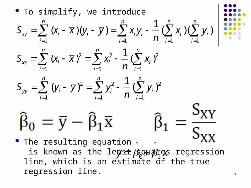
To simplify, we introduce

The resulting equation is known as the least squares regression line, which is an estimate of the true regression line.

1 1 1 1

2 2 2

1 1 1

2 2 2

1 1 1

1( )( ) ( )( )

1( ) ( )

1( ) ( )

n n n n

xy i i i i i ii i i i

n n n

xx i i ii i i

n n n

yy i i ii i i

S x x y y x y x yn

S x x x xn

S y y y yn

0 1y x

17

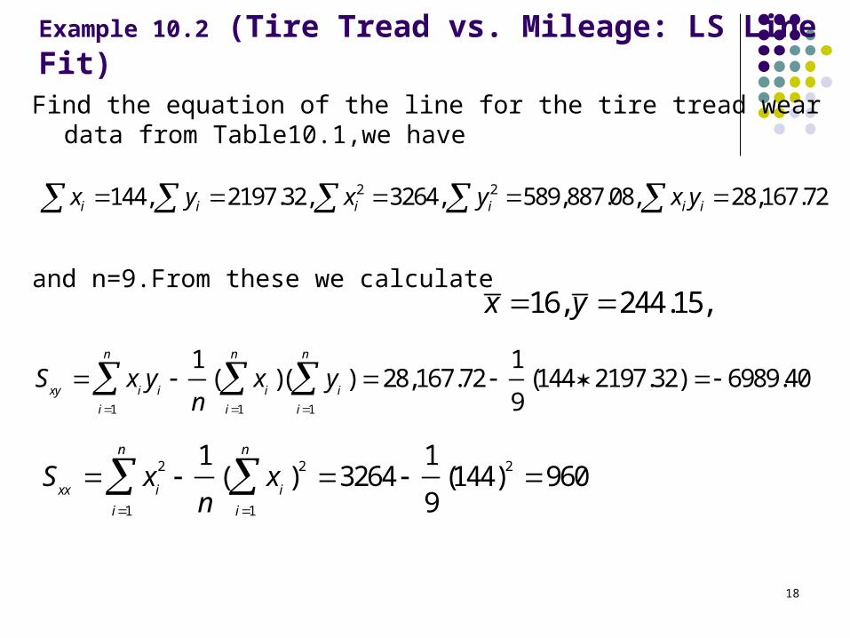
Example 10.2 (Tire Tread vs. Mileage: LS Line Fit)Find the equation of the line for the tire tread wear data from

Table10.1,we have

and n=9.From these we calculate

2 2144, 2197.32, 3264, 589,887.08, 28,167.72i i i i i ix y x y x y

16, 244.15,x y

1 1 1

1 1( )( ) 28,167.72 (144 2197.32) 6989.40

9

n n n

xy i i i i

i i i

S x y x yn

2 2 2

1 1

1 1( ) 3264 (144) 960

9

n n

xx i i

i i

S x xn

18

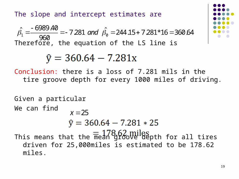
The slope and intercept estimates are

Therefore, the equation of the LS line is

Conclusion: there is a loss of 7.281 mils in the tire groove depth for every 1000 miles of driving.

Given a particular

We can find

This means that the mean groove depth for all tires driven for 25,000miles is estimated to be 178.62 miles.

1 0

6989.40ˆ ˆ7.281 244.15 7.281*16 360.64960

and

25x

19

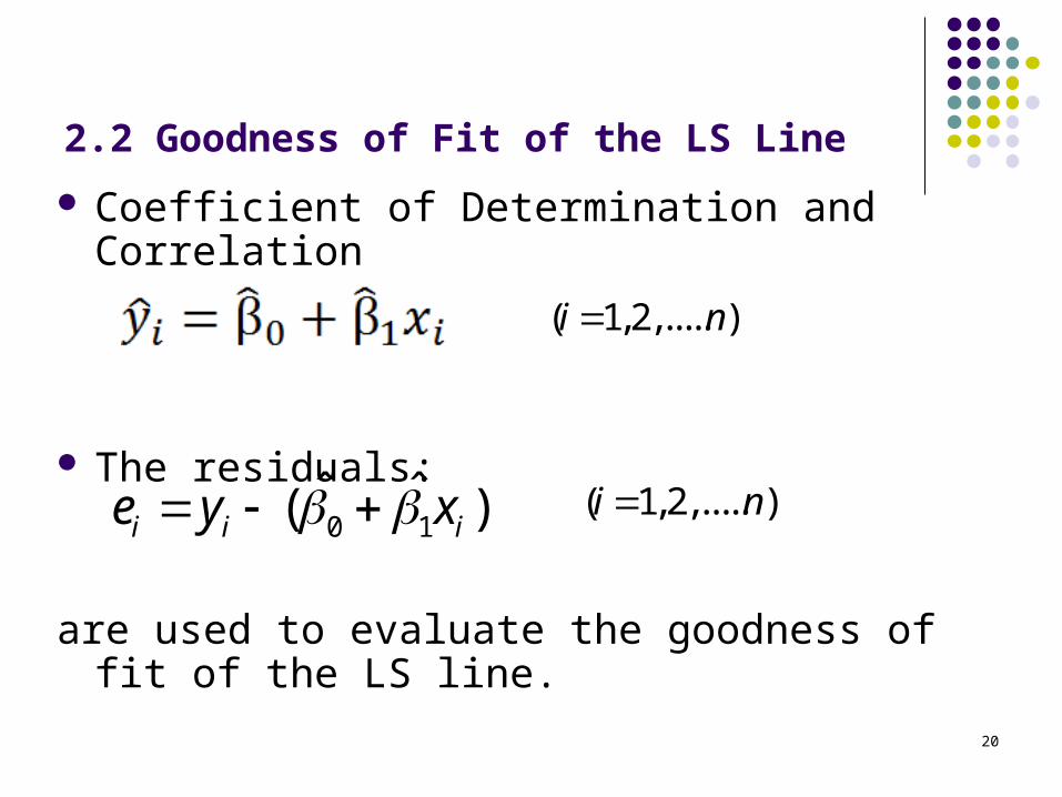
2.2 Goodness of Fit of the LS Line

Coefficient of Determination and Correlation

The residuals:

are used to evaluate the goodness of fit of the LS line.

( 1,2,..... )i n

0 1ˆ ˆ( )i i ie y x ( 1,2,..... )i n

20

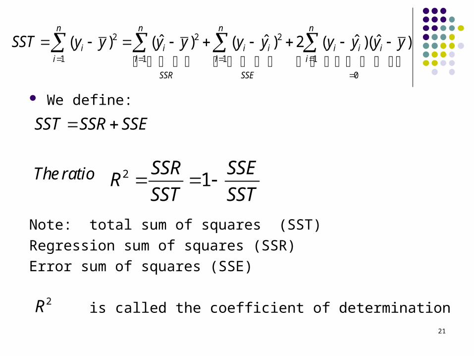
We define:

Note: total sum of squares (SST)

Regression sum of squares (SSR)

Error sum of squares (SSE)

is called the coefficient of determination

2 2 2

1 1 1 1

0

ˆ ˆ ˆ ˆ( ) ( ) ( ) 2 ( )( )n n n n

i i i i i i ii i i i

SSR SSE

SST y y y y y y y y y y

SST SSR SSE

The ratio

2 1SSR SSE

RSST SST

21

2R

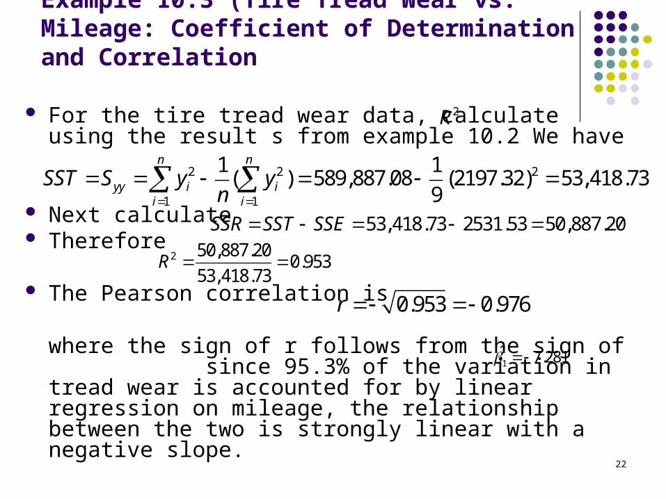
Example 10.3 (Tire Tread Wear vs. Mileage: Coefficient of Determination and Correlation

For the tire tread wear data, calculate using the result s from example 10.2 We have

Next calculate Therefore

The Pearson correlation is

where the sign of r follows from the sign of since 95.3% of the variation in tread wear is accounted for by linear regression on mileage, the relationship between the two is strongly linear with a negative slope.

2 2 2

1 1

1 1( ) 589,887.08 (2197.32) 53,418.73

9

n n

yy i ii i

SST S y yn

53,418.73 2531.53 50,887.20SSR SST SSE

2 50,887.200.953

53,418.73R

1̂ 7.281

2R

22

0.953 0.976r

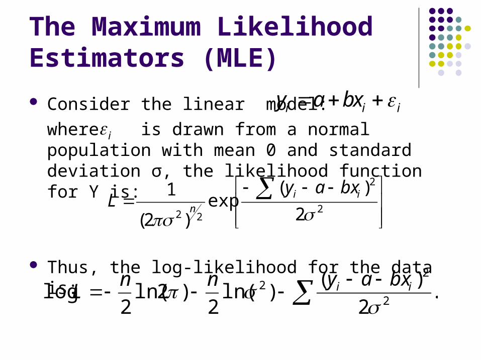
The Maximum Likelihood Estimators (MLE)

Consider the linear model:

where is drawn from a normal population with mean 0 and standard deviation σ, the likelihood function for Y is:

Thus, the log-likelihood for the data is:

i i iy a bx i

2

2

22 2

)(exp

)2(

1

ii

n

bxayL

.2

)()ln(

2)2ln(

2log

2

22

ii bxaynn

L

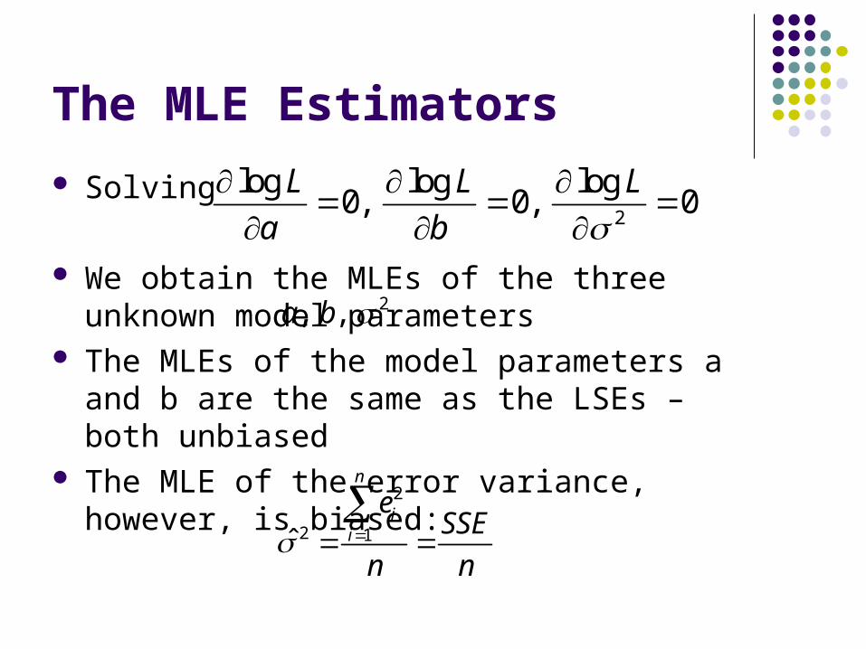
The MLE Estimators

Solving

We obtain the MLEs of the three unknown model parameters

The MLEs of the model parameters a and b are the same as the LSEs – both unbiased

The MLE of the error variance, however, is biased:

2, ,a b

2

log log log0, 0, 0

L L L

a b

2

2 1ˆ

n

ii

eSSE

n n

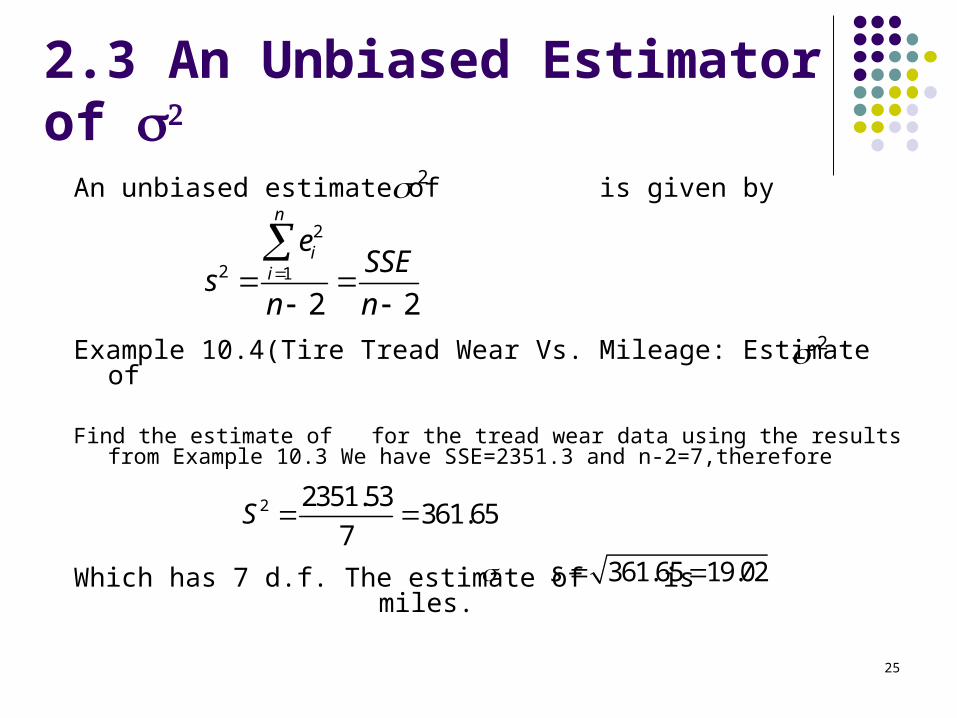
2.3 An Unbiased Estimator of

An unbiased estimate of is given by

Example 10.4(Tire Tread Wear Vs. Mileage: Estimate of

Find the estimate of for the tread wear data using the results from Example 10.3 We have SSE=2351.3 and n-2=7,therefore

Which has 7 d.f. The estimate of is miles.

22

2 1

2 2

n

ii

eSSE

sn n

2

2 2351.53361.65

7S

361.65 19.02s

25

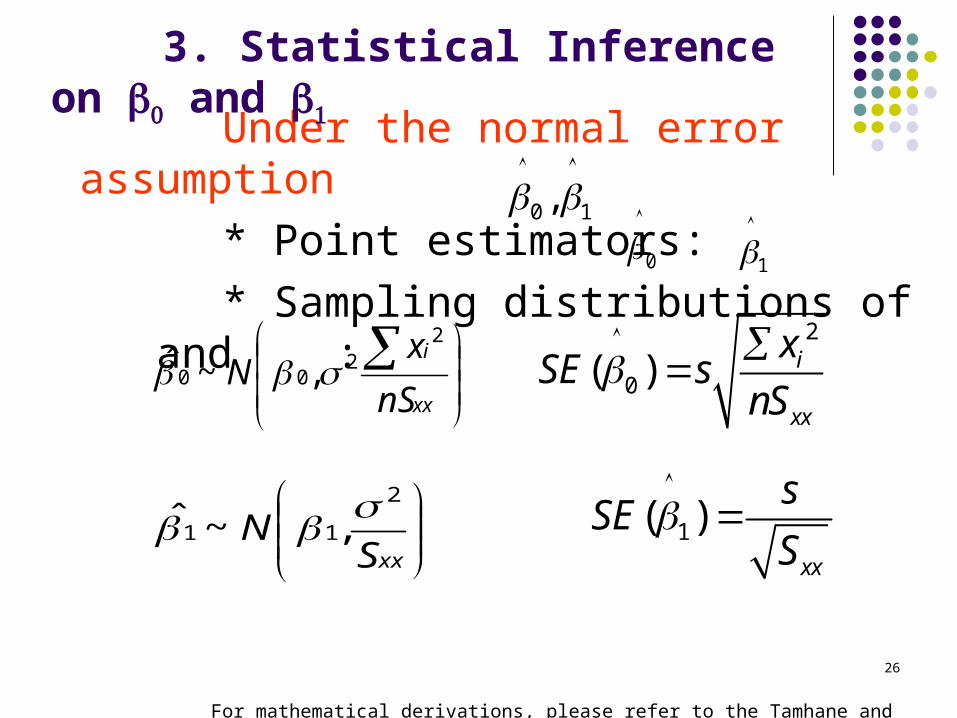
Under the normal error assumption

* Point estimators:

* Sampling distributions of and :

For mathematical derivations, please refer to the Tamhane and Dunlop text book, P331.

1

00 1,

2

0( ) i

xx

xSE s

nS

1( )xx

sSE

S

xx

i

nS

xN

22

00 ,~ˆ

xxS

N2

11 ,~ˆ

3. Statistical Inference on and

26

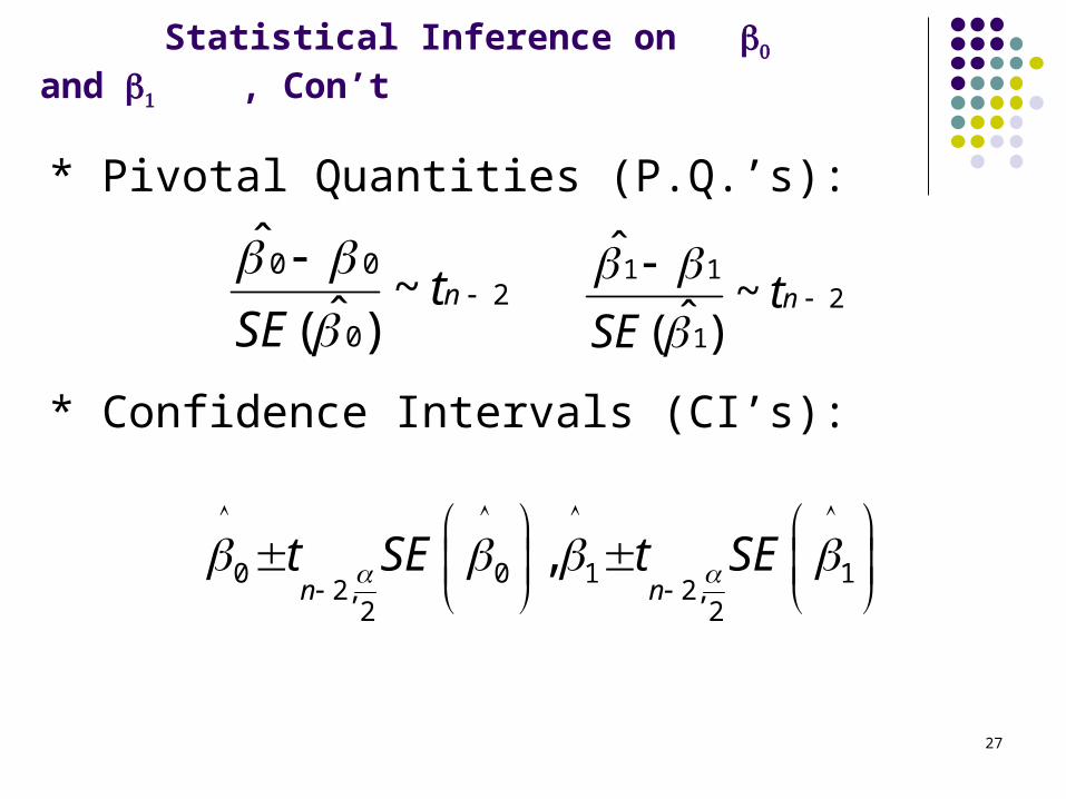
* Pivotal Quantities (P.Q.’s):

* Confidence Intervals (CI’s):

0 0 1 12, 2,

2 2

,n n

t SE t SE

2

0

00~

)ˆ(

ˆ

nt

SE

2

1

11~

)ˆ(

ˆ

nt

SE

27

Statistical Inference on and , Con’t

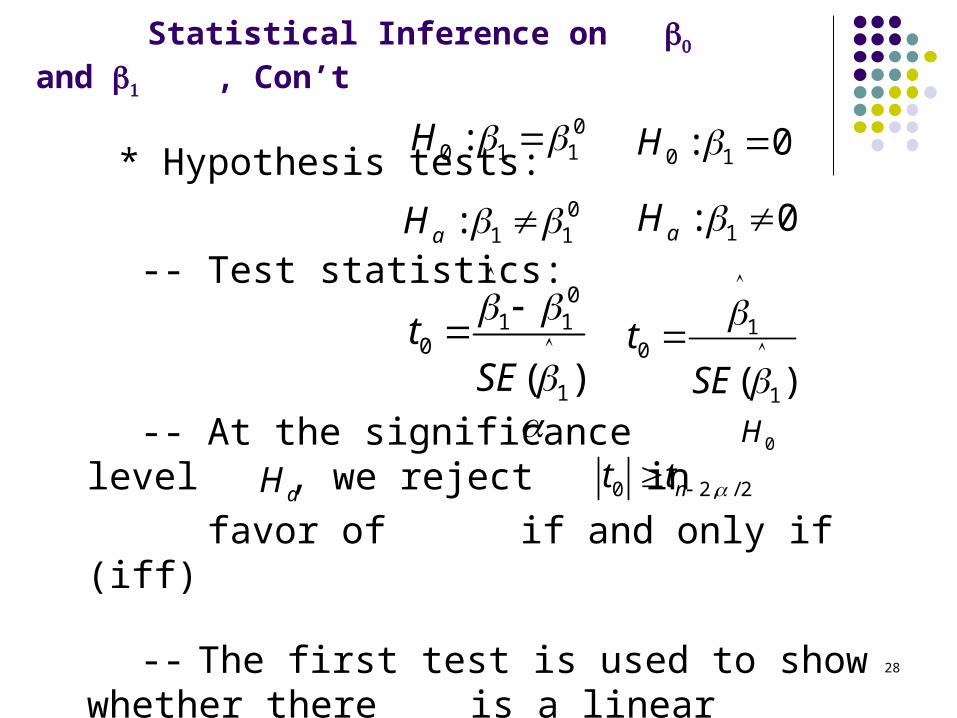
* Hypothesis tests:

-- Test statistics:

-- At the significance level , we reject in

favor of if and only if (iff)

-- The first test is used to show whether there is a linear relationship between x and y

aH0H

00 1 1:H

01 1:aH

01 1

0

1( )t

SE

0 2, / 2nt t

0 1: 0H

1: 0aH

10

1( )t

SE

Statistical Inference on and , Con’t

28

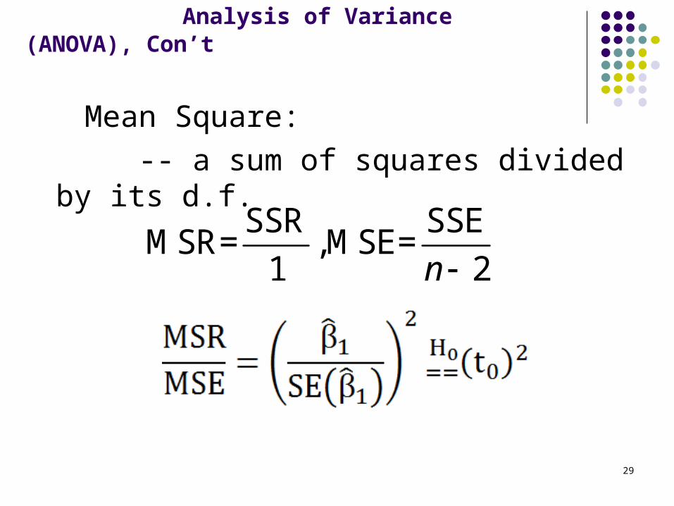
Analysis of Variance (ANOVA), Con’t

Mean Square:

-- a sum of squares divided by its d.f.

SSR SSEMSR= ,MSE=

1 2n

29

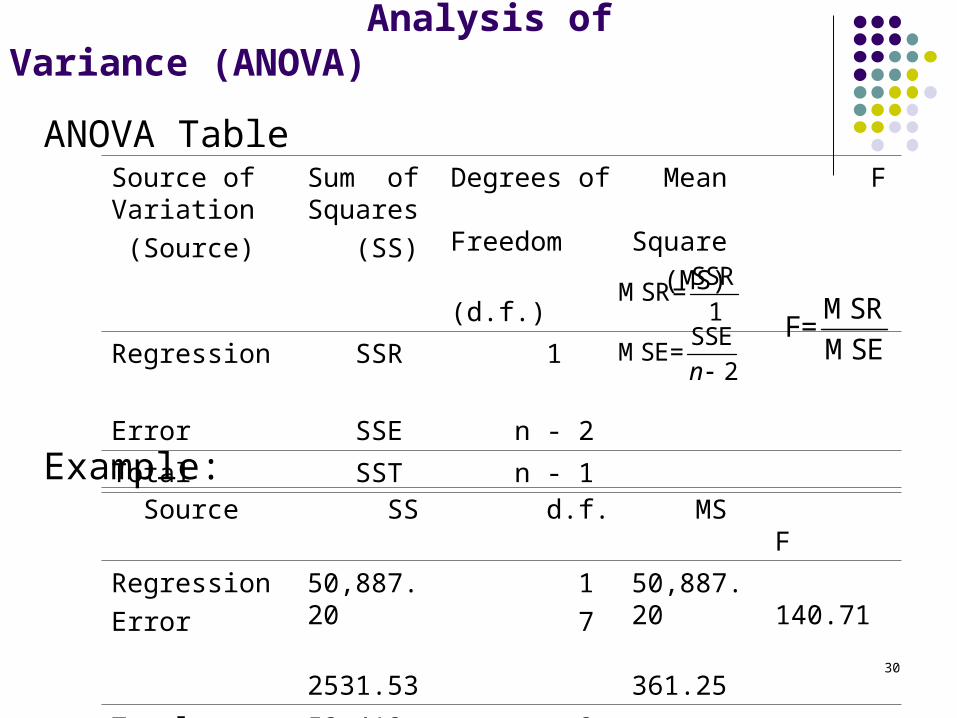
Analysis of Variance (ANOVA)

ANOVA Table

Example:

Source of Variation

(Source)

Sum of Squares

(SS)

Degrees of Freedom

(d.f.)

Mean Square

(MS)

F

Regression

Error

SSR

SSE

1

n - 2

Total SST n - 1

SSRMSR=

1SSE

MSE=2n

MSRF=

MSE

Source SS d.f. MS F

Regression

Error

50,887.20

2531.53

1

7

50,887.20

361.25

140.71

Total 53,418.73

8 30

31

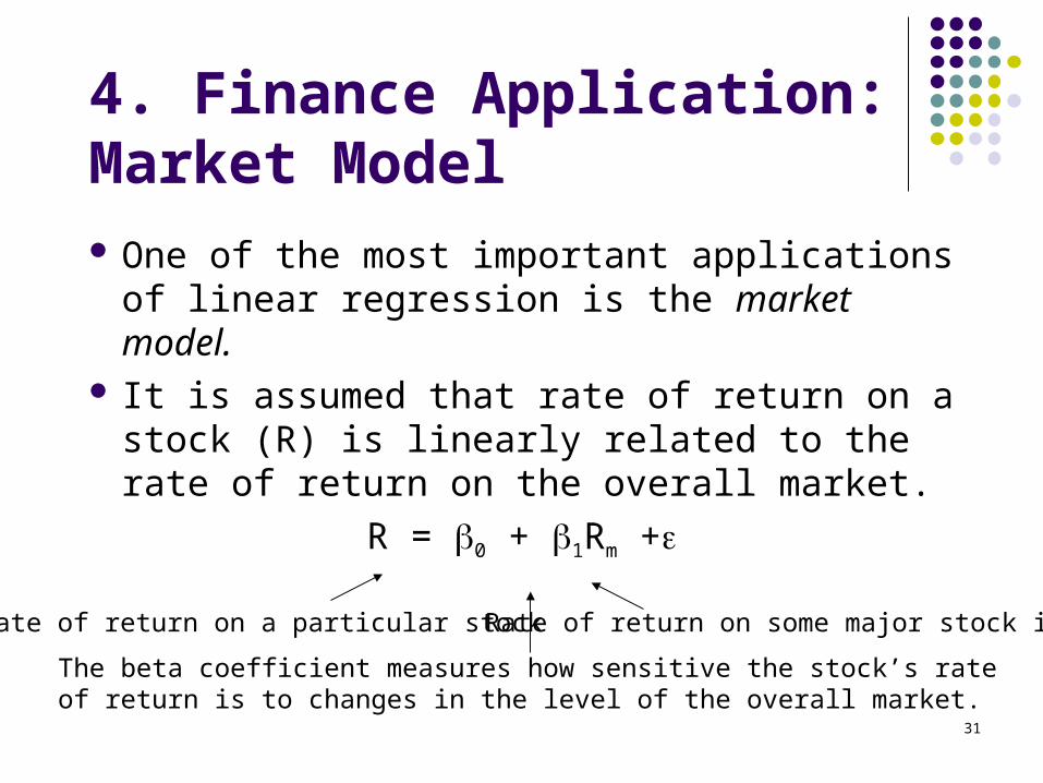
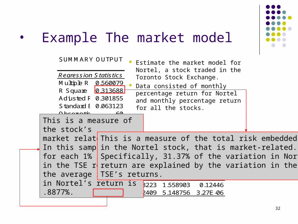
4. Finance Application: Market Model

One of the most important applications of linear regression is the market model.

It is assumed that rate of return on a stock (R) is linearly related to the rate of return on the overall market.

R = 0 + 1Rm +

Rate of return on a particular stock Rate of return on some major stock index

The beta coefficient measures how sensitive the stock’s rate of return is to changes in the level of the overall market.

32

• Example The market modelSUMMARY OUTPUT

Regression StatisticsMultiple R 0.560079R Square 0.313688Adjusted R Square0.301855Standard Error0.063123Observations 60

ANOVAdf SS MS F Significance F

Regression 1 0.10563 0.10563 26.50969 3.27E-06Residual 58 0.231105 0.003985Total 59 0.336734

CoefficientsStandard Error t Stat P-valueIntercept 0.012818 0.008223 1.558903 0.12446TSE 0.887691 0.172409 5.148756 3.27E-06

Estimate the market model for Nortel, a stock traded in the Toronto Stock Exchange.

Data consisted of monthly percentage return for Nortel and monthly percentage returnfor all the stocks.

This is a measure of the stock’smarket related risk. In this sample, for each 1% increase in the TSE return, the average increase in Nortel’s return is .8877%.

This is a measure of the total risk embeddedin the Nortel stock, that is market-related.Specifically, 31.37% of the variation in Nortel’sreturn are explained by the variation in the TSE’s returns.

5. Regression Diagnostics

5.1 Checking for Model Assumptions

Checking for Linearity Checking for Constant Variance Checking for Normality Checking for Independence

33

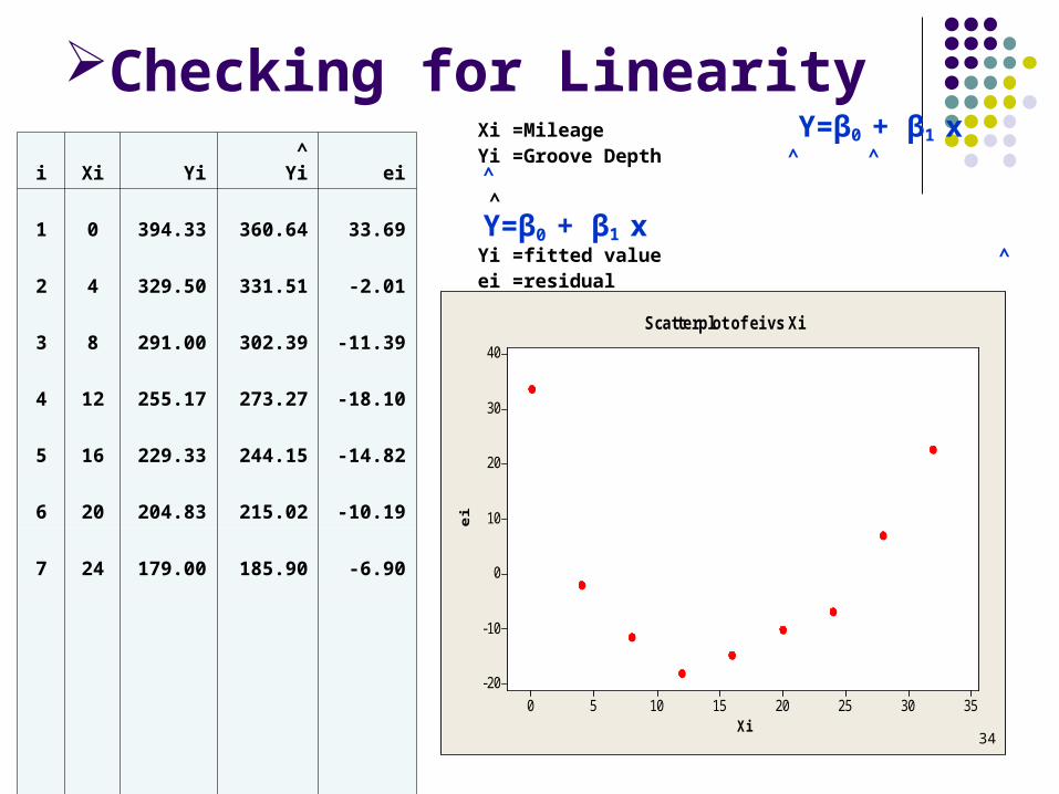
Checking for Linearity Xi =Mileage Y=β0 + β1 x Yi =Groove Depth ^ ^ ^

^ Y=β0 + β1 x Yi =fitted value ^

ei =residual Residual = ei = Yi- Yi

i Xi Yi^

Yi ei

1 0 394.33 360.64 33.69

2 4 329.50 331.51 -2.01

3 8 291.00 302.39 -11.39

4 12 255.17 273.27 -18.10

5 16 229.33 244.15 -14.82

6 20 204.83 215.02 -10.19

7 24 179.00 185.90 -6.90

8 28 163.83 156.78 7.05

9 32 150.33 127.66 22.67

Xi

ei

35302520151050

40

30

20

10

0

-10

-20

Scatterplot of ei vs Xi

34

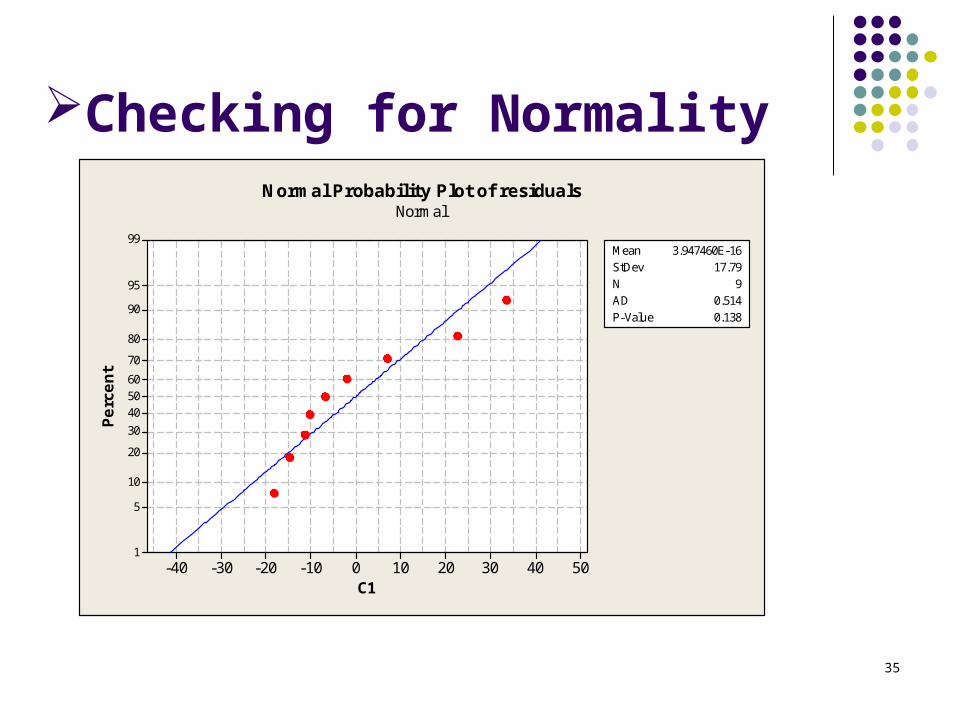
Checking for Normality

C1

Perc

ent

50403020100-10-20-30-40

99

95

90

80

70

605040

30

20

10

5

1

Mean 3.947460E-16StDev 17.79N 9AD 0.514P-Value 0.138

Normal Probability Plot of residualsNormal　

35

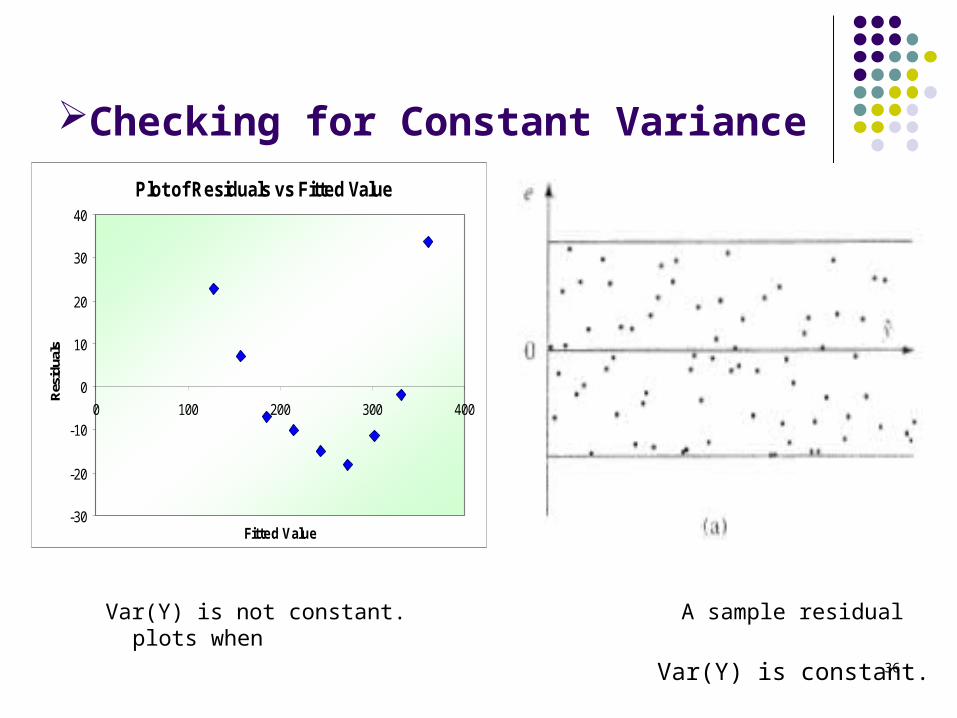
Checking for Constant Variance

Var(Y) is not constant. A sample residual plots when

Var(Y) is constant.

Plot of Residuals vs Fitted Value

-30

-20

-10

0

10

20

30

40

0 100 200 300 400

Fitted Value

Res

idua

ls

36

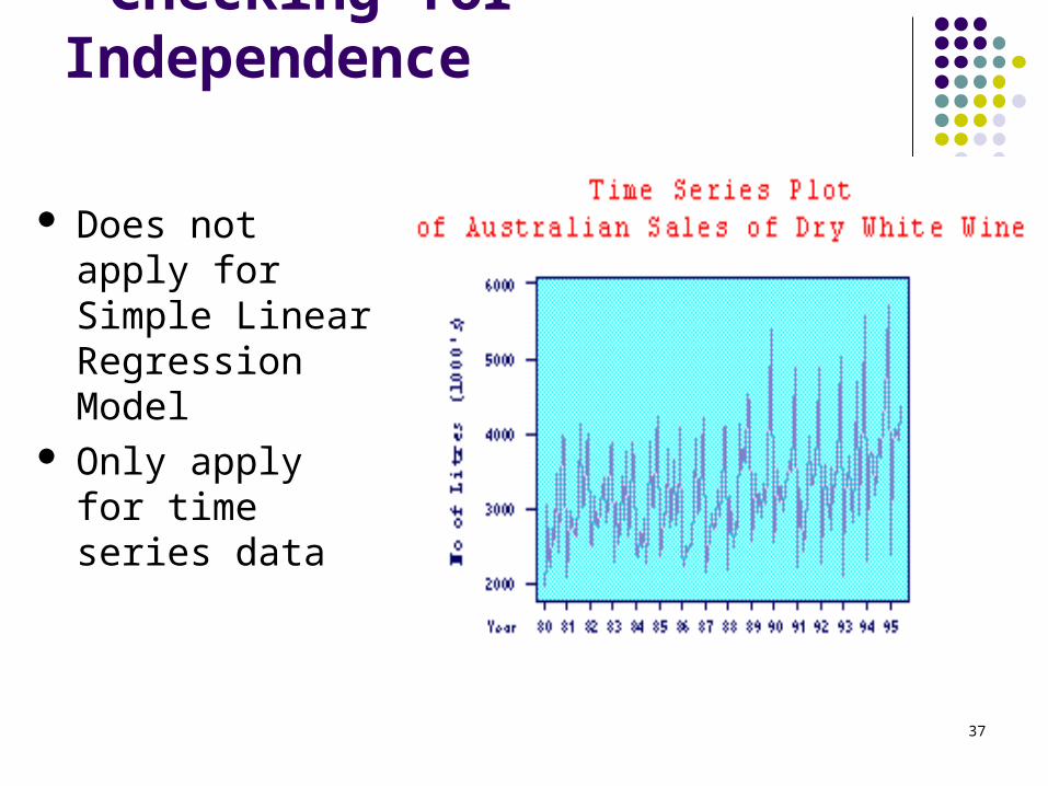
Checking for Independence

Does not apply for Simple Linear Regression Model

Only apply for time series data

37

5.2 Checking for Outliers & Influential Observations

What is OUTLIER Why checking for outliers is important Mathematical definition How to deal with them

38

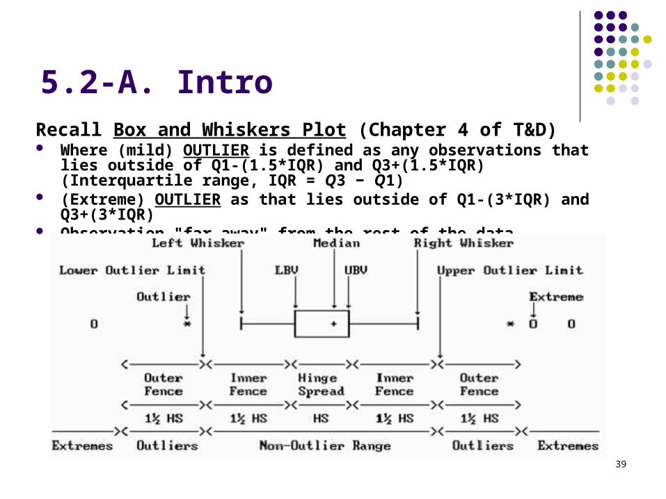
5.2-A. IntroRecall Box and Whiskers Plot (Chapter 4 of T&D) Where (mild) OUTLIER is defined as any observations that lies outside of

Q1-(1.5*IQR) and Q3+(1.5*IQR) (Interquartile range, IQR = Q3 − Q1) (Extreme) OUTLIER as that lies outside of Q1-(3*IQR) and Q3+(3*IQR) Observation "far away" from the rest of the data

39

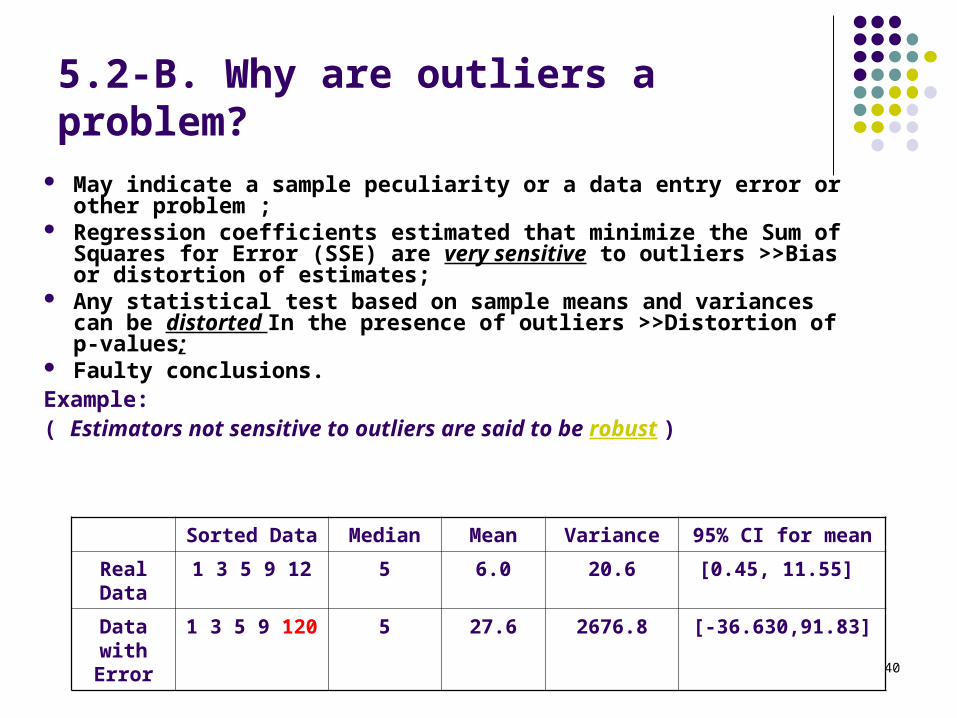
5.2-B. Why are outliers a problem?

May indicate a sample peculiarity or a data entry error or other problem ;

Regression coefficients estimated that minimize the Sum of Squares for Error (SSE) are very sensitive to outliers >>Bias or distortion of estimates;

Any statistical test based on sample means and variances can be distorted In the presence of outliers >>Distortion of p-values;

Faulty conclusions.Example: ( Estimators not sensitive to outliers are said to be robust )

Sorted Data Median Mean Variance 95% CI for mean

Real Data

1 3 5 9 12 5 6.0 20.6 [0.45, 11.55]

Data with Error

1 3 5 9 120 5 27.6 2676.8 [-36.630,91.83]

40

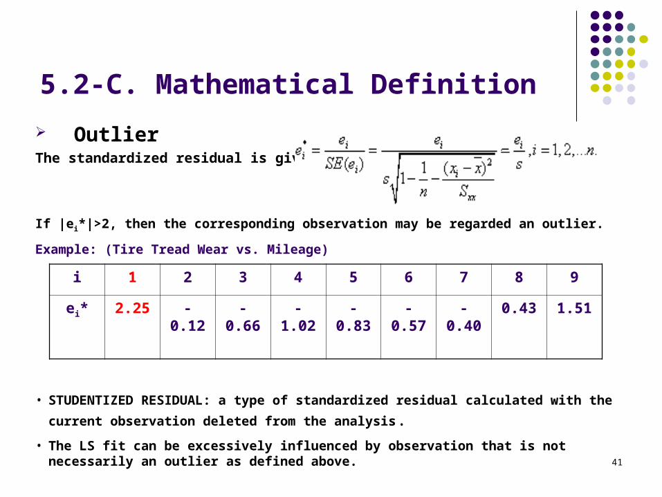
5.2-C. Mathematical Definition

OutlierThe standardized residual is given by

If |ei*|>2, then the corresponding observation may be regarded an outlier.

Example: (Tire Tread Wear vs. Mileage)

• STUDENTIZED RESIDUAL: a type of standardized residual calculated with the current

observation deleted from the analysis.• The LS fit can be excessively influenced by observation that is not necessarily an outlier as

defined above.

i 1 2 3 4 5 6 7 8 9

ei* 2.25 -0.12 -0.66 -1.02 -0.83 -0.57 -0.40 0.43 1.51

41

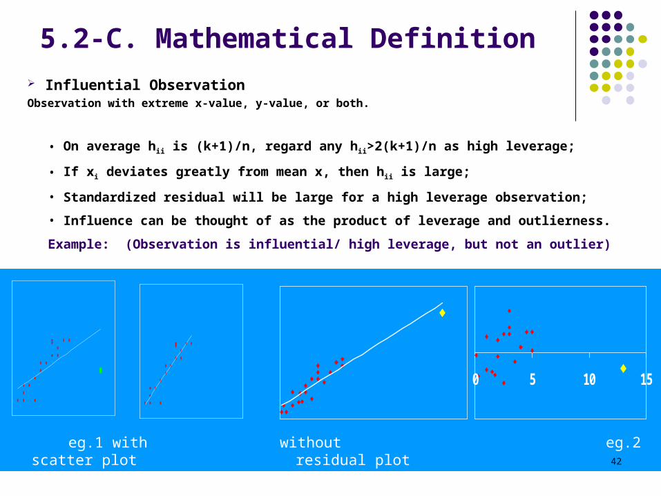
5.2-C. Mathematical Definition Influential ObservationObservation with extreme x-value, y-value, or both.

• On average hii is (k+1)/n, regard any hii>2(k+1)/n as high leverage;

• If xi deviates greatly from mean x, then hii is large;

• Standardized residual will be large for a high leverage observation;

• Influence can be thought of as the product of leverage and outlierness.

Example: (Observation is influential/ high leverage, but not an outlier)

eg.1 with without eg.2 scatter plot residual plot

0 5 10 15

42

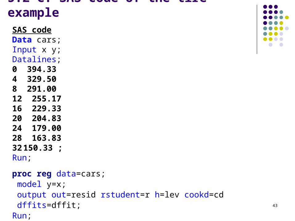
5.2-C. SAS code of the tire exampleSAS codeData cars;Input x y;Datalines;0 394.334 329.508 291.0012 255.1716 229.3320 204.8324 179.0028 163.8332 150.33 ;Run;

proc reg data=cars; model y=x; output out=resid rstudent=r h=lev cookd=cd dffits=dffit;Run;

43

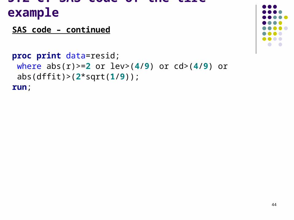
5.2-C. SAS code of the tire exampleSAS code – continued

proc print data=resid; where abs(r)>=2 or lev>(4/9) or cd>(4/9) or abs(dffit)>(2*sqrt(1/9)); run;

44

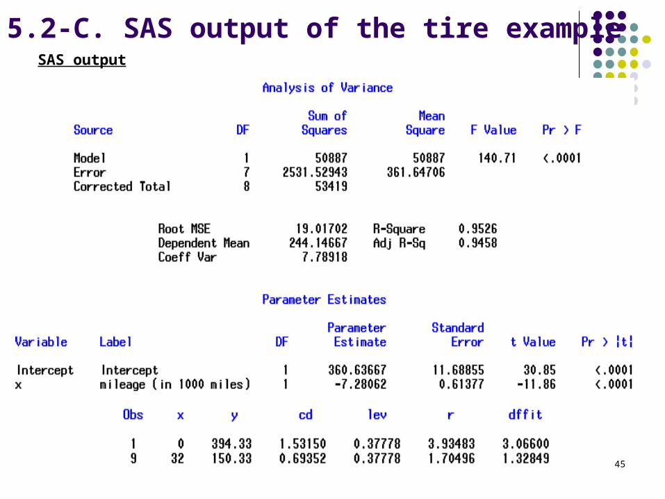
5.2-C. SAS output of the tire exampleSAS output

45

5.2-D. How to deal with Outliers & Influential Observations

Investigate (Data errors? Rare events? Can be corrected?)

Ways to accommodate outliers Non Parametric Methods (robust to outliers) Data Transformations Deletion (or report model results both with and

without the outliers or influential observations to see how much they change)

46

5.3 Data Transformations

Reason

To achieve linearity To achieve homogeneity of variance To achieve normality or symmetry about the

regression equation

47

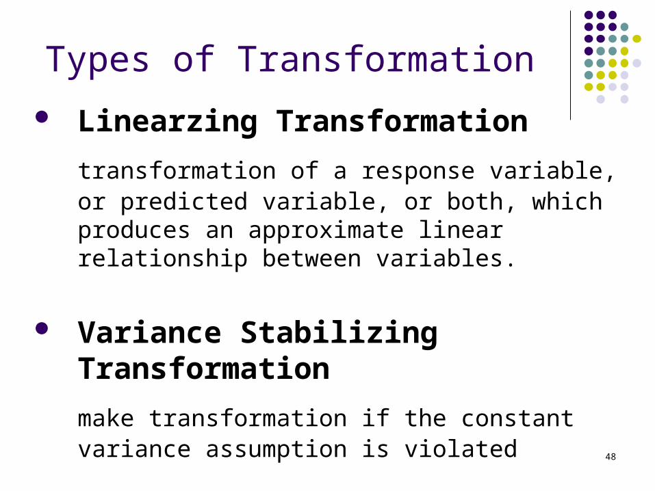
Types of Transformation

Linearzing Transformation

transformation of a response variable, or predicted variable, or both, which produces an approximate linear relationship between variables.

Variance Stabilizing Transformation

make transformation if the constant variance assumption is violated

48

Linearizing Transformation

Use mathematical operation, e.g. square root, power, log, exponential, etc.

Only one variable needs to be transformed in the simple linear regression.

Which one? Predictor or Response? Why?

49

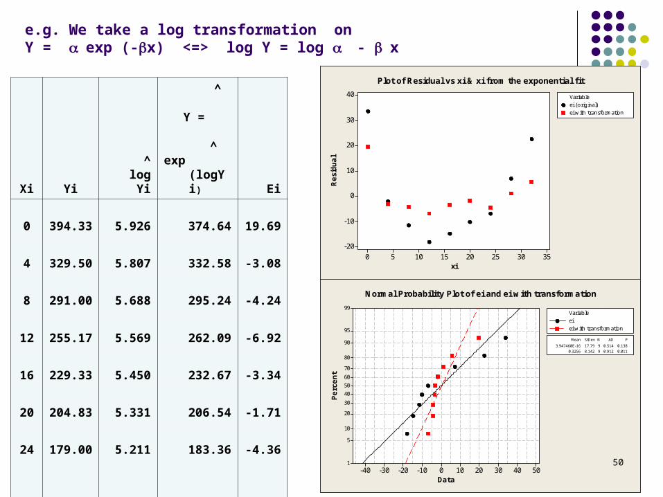
Xi Yi^

log Yi

^ Y =

^exp (logYi) Ei

0 394.33 5.926 374.64 19.69

4 329.50 5.807 332.58 -3.08

8 291.00 5.688 295.24 -4.24

12 255.17 5.569 262.09 -6.92

16 229.33 5.450 232.67 -3.34

20 204.83 5.331 206.54 -1.71

24 179.00 5.211 183.36 -4.36

28 163.83 5.092 162.77 1.06

32 150.33 4.973 144.50 5.83

e.g. We take a log transformation on Y = exp (-x) <=> log Y = log - x

xi

Resi

dual

35302520151050

40

30

20

10

0

-10

-20

ei　(original)ei　with　transformation

Variable

Plot of Residual vs xi & xi from the exponential fit

Data

Perc

ent

50403020100-10-20-30-40

99

95

90

80

70

60

50

40

30

20

10

5

1

3.947460E-16 17.79 9 0.514 0.1380.3256 8.142 9 0.912 0.011

Mean StDev N AD P

eiei　with　transformation

Variable

Normal Probability Plot of ei and ei with transformation

50

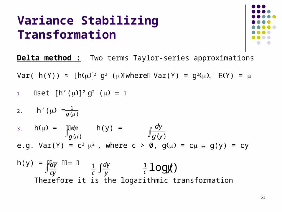
Variance Stabilizing Transformation

Delta method : Two terms Taylor-series approximations

Var( h(Y)) ≈ [h2 g2 (whereVar(Y) = g2Y) =

. set [h’(]2 g2 (

2. h’( =

3. h =  h(y) =

e.g. Var(Y) = c22 , where c > 0, g = c↔ g(y) = cy

h(y) =

Therefore it is the logarithmic transformation

)(

g

d

)(yg

dy

)(1g

cydy y

dyc 1 )log(1 yc

51

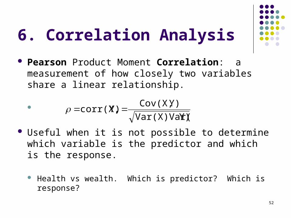
6. Correlation Analysis

Pearson Product Moment Correlation: a measurement of how closely two variables share a linear relationship.

Useful when it is not possible to determine which variable is the predictor and which is the response.

Health vs wealth. Which is predictor? Which is response?

Y)Var(X)Var(

Y) Cov(X, Y) corr(X,

52

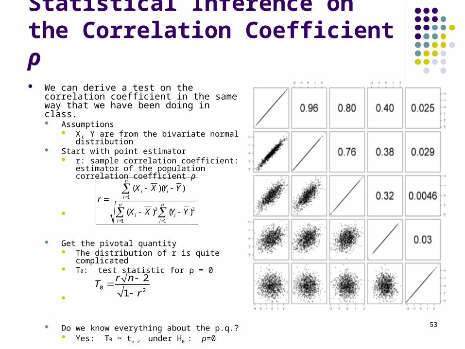
Statistical Inference on the Correlation Coefficient ρ We can derive a test on the correlation

coefficient in the same way that we have been doing in class. Assumptions

X, Y are from the bivariate normal distribution

Start with point estimator r: sample correlation coefficient: estimator

of the population correlation coefficient ρ

Get the pivotal quantity The distribution of r is quite complicated T0: test statistic for ρ = 0

Do we know everything about the p.q.? Yes: T0 ~ tn-2 under H0 : ρ=0

1

2 2

1 1

( )( )

( ) ( )

n

i ii

n n

i ii i

X X Y Yr

X X Y Y

0 2

2

1

r nT

r

53

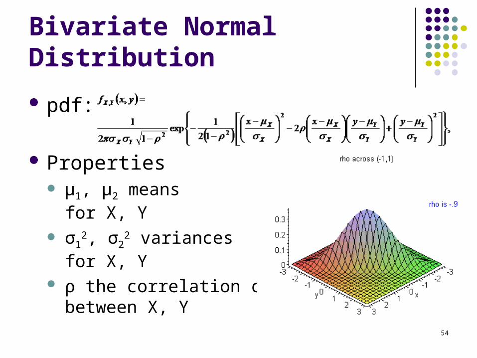
Bivariate Normal Distribution

pdf:

Properties μ1, μ2 means

for X, Y σ1

2, σ22 variances

for X, Y ρ the correlation coeff

between X, Y54

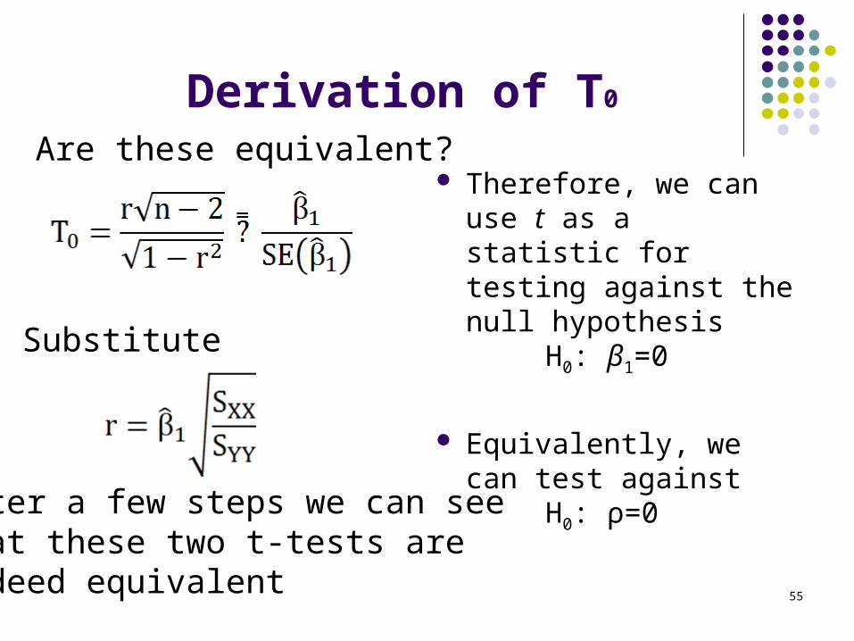
Derivation of T0

Therefore, we can use t as a statistic for testing against the null hypothesis

H0: β1=0

Equivalently, we can test against

H0: ρ=0

55

Are these equivalent?

Substitute

After a few steps we can see that these two t-tests are indeed equivalent

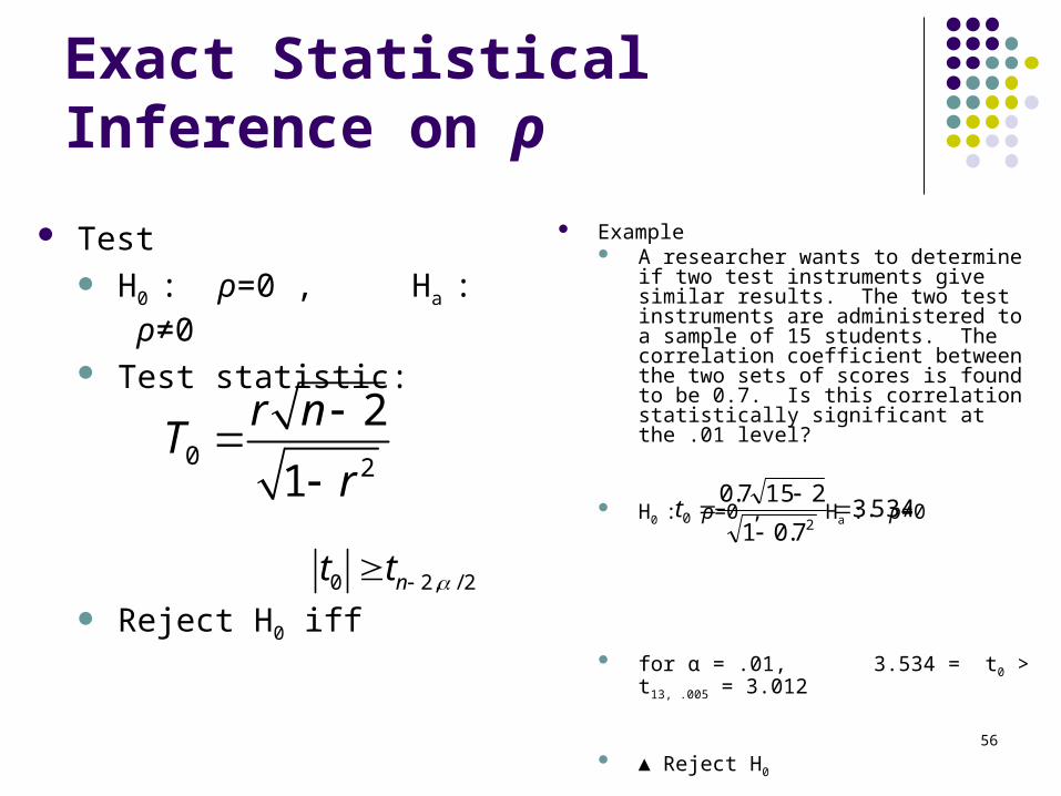
Exact Statistical Inference on ρ

Test H0 : ρ=0 , Ha : ρ≠0 Test statistic:

Reject H0 iff

0 2

2

1

r nT

r

534.3

7.01

2157.020

t

Example A researcher wants to determine if two test

instruments give similar results. The two test instruments are administered to a sample of 15 students. The correlation coefficient between the two sets of scores is found to be 0.7. Is this correlation statistically significant at the .01 level?

H0 : ρ=0 , Ha : ρ≠0

for α = .01, 3.534 = t0 > t13, .005 = 3.012

▲ Reject H0

56

0 2, / 2nt t

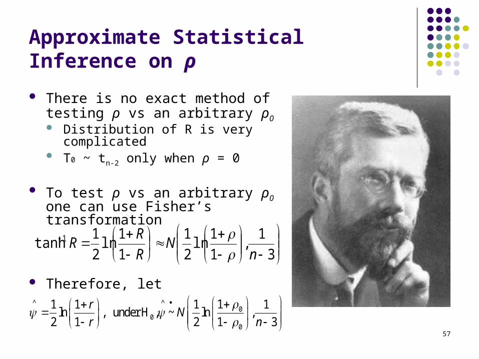
Approximate Statistical Inference on ρ

There is no exact method of testing ρ vs an arbitrary ρ0 Distribution of R is very

complicated T0 ~ tn-2 only when ρ = 0

To test ρ vs an arbitrary ρ0 one can use Fisher’s transformation

Therefore, let

3

1,

1

1ln

2

1

1

1ln

2

1tanh 1

nN

R

RR

^ ^0

00

11 1 1 1ln , under H , ~ ln ,

2 1 2 1 3

rN

r n

57

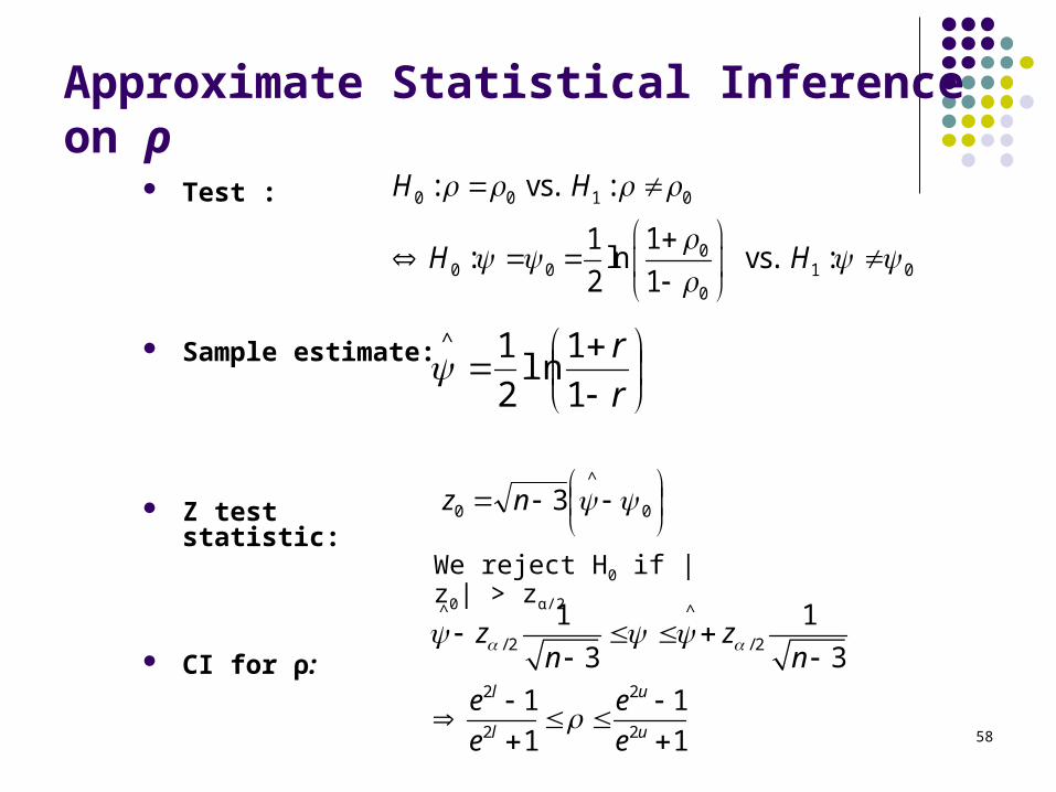
Approximate Statistical Inference on ρ Test :

Sample estimate:

Z test statistic:

CI for ρ:

r

r

1

1ln

2

1^

0

^

0 3 nz

0 0 1 0

00 0 1 0

0

: vs. :

11: ln vs. :

2 1

H H

H H

^ ^

/ 2 / 2

2 2

2 2

1 1

3 3

1 1

1 1

l u

l u

z zn n

e e

e e

We reject H0 if |z0| > zα/2

58

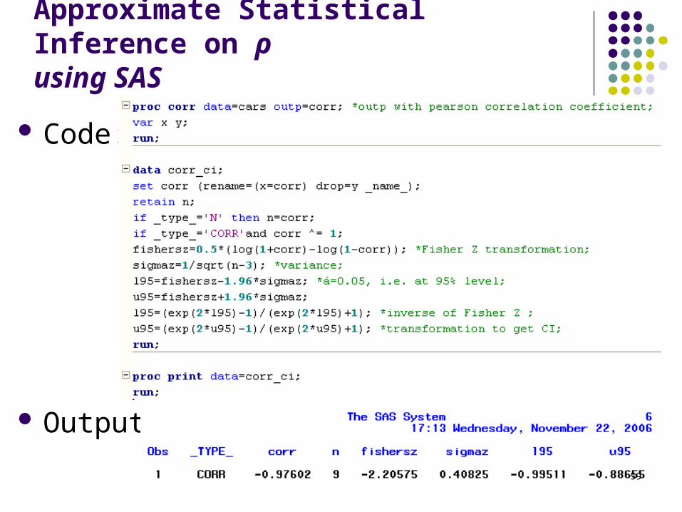
Approximate Statistical Inference on ρusing SAS

Code:

Output:

59

Pitfalls of Regression and Correlation Analysis

Correlation and causation Ticks cause good health

Coincidental data Sun spots and republicans

Lurking variables Church, suicide, population

Restricted range Local, global linearity

60

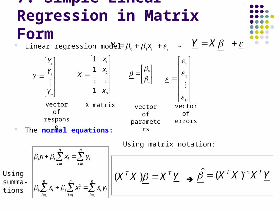
7. Simple Linear Regression in Matrix Form

iii xY 10

Linear regression model

The normal equations:

XY

nY

Y

Y

Y

2

1

nx

x

x

X

1

1

1

2

1

1

0

n

2

1

vector ofresponse

X matrix vector oferrors

vector ofparameters

YXXX TT 1)(ˆ

n

iii

n

ii

n

ii

n

ii

n

ii

yxxx

yxn

11

2

1

1

0

11

10

Using summa-tions

Using matrix notation:

→

YXXX TT )(

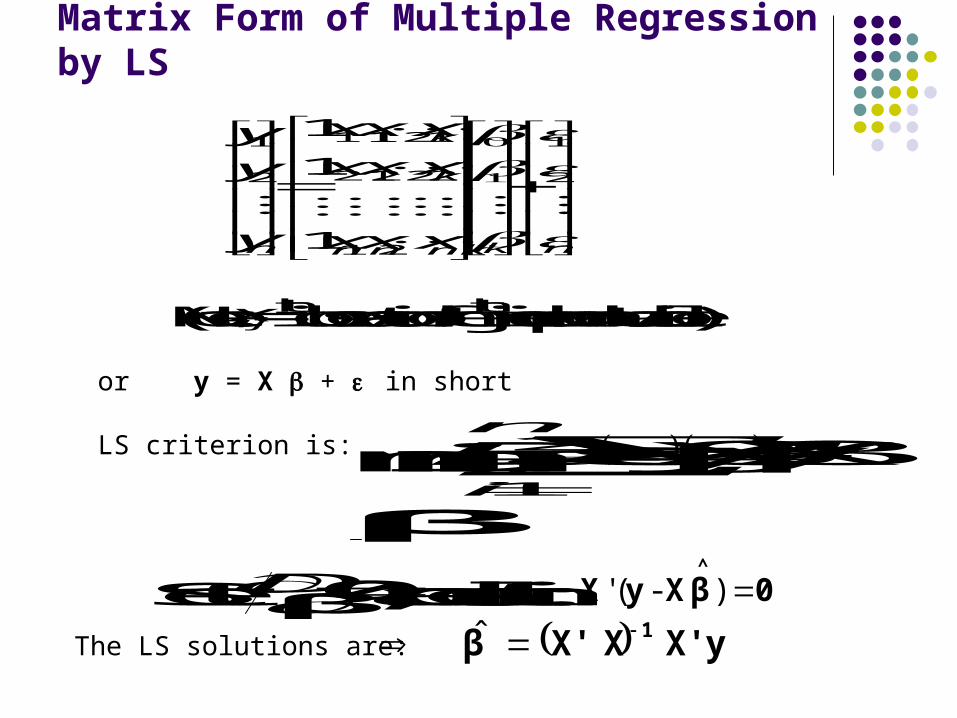
Matrix Form of Multiple Regression by LS

nknknn

k

k

n xxx

xxx

xxx

y

y

y

2

1

21

22221

11211

2

1

1

1

1

(Note: ijx= i

th observation of the jth independent variable)

or y = X + in short

LS criterion is: min β X -y 'βX -y ε ε' 1

2

n

iiD

β

Set 0β D , and result in: 0β XyX

^

) - ( '

The LS solutions are: y X' XX' β 1 ˆ

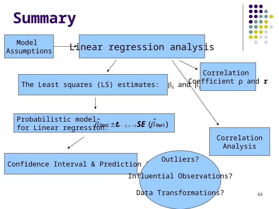
Summary

Linear regression analysis

The Least squares (LS) estimates: and

Correlation Coefficient ρ and r

Probabilistic model for Linear regression:

Confidence Interval & Prediction intervalOutliers?

Influential Observations?

Data Transformations?

CorrelationAnalysis

Model Assumptions

)ˆ(ˆ 1010 2/,2 oror SEtn

63

2

2

1

r nt

r

1 1ln

2 1

2 1SSR SSE

rSST SST

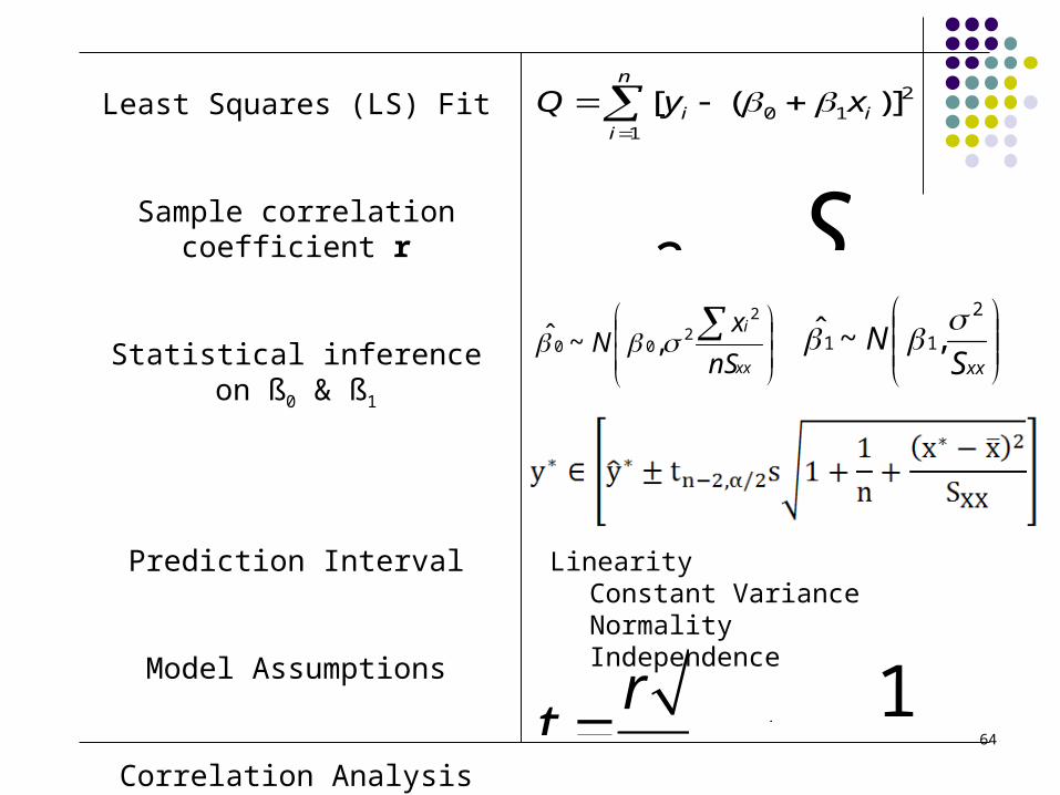
20 1

1

[ ( )]n

i ii

Q y x

Least Squares (LS) Fit

Sample correlation coefficient r

Statistical inference on ß0 & ß1

Prediction Interval

Model Assumptions

Correlation Analysis

Linearity Constant Variance Normality Independence

xx

i

nS

xN

22

00 ,~ˆ

xxS

N2

11 ,~ˆ

64

65

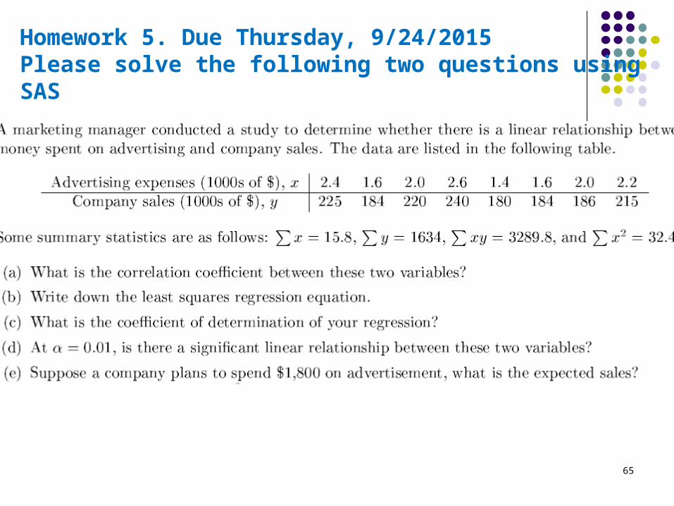
Homework 5. Due Thursday, 9/24/2015Please solve the following two questions using SAS

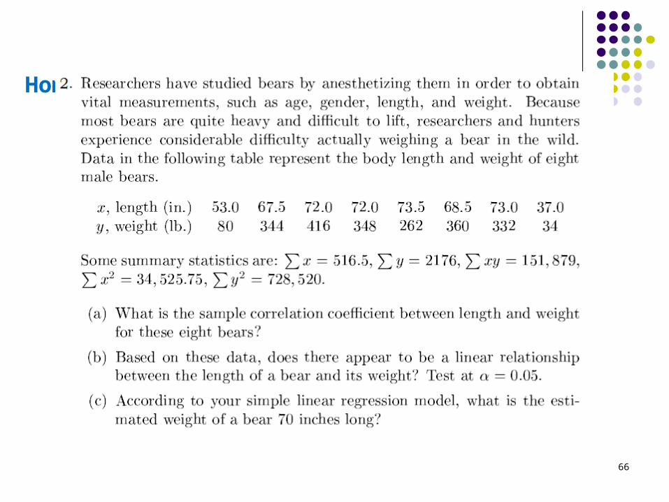
Homework 5. Continued

66