1

Paper 1815-2018

Simple Methods for Repeatability and Comparability: Bland-Altman Plots, Bias, and Measurement Error

Maribeth Johnson and Jennifer Waller

Augusta University ABSTRACT While a Pearson correlation coefficient may be a quick and easy measure to compare two different measurement methods or examine repeatability of a measure it is not the most appropriate nor does it give you insight into bias. Additionally, performing linear regression or tests for differences between the means is also not the best approach for determining whether two methods are comparable or a measurement is repeatable. Examining the difference between the measurements may not offer insight into the accuracy of the methods and a Pearson product moment correlation coefficient is not a measure of agreement but a measure of association. Altman and Bland (1983) suggested a graphical method and two other statistical tests to examine repeatability of measurement or whether two methods of measurement produced similar results. The graphical method, called a Bland-Altman plot, is a plot of the difference versus the average of two different measures with y-reference lines at ±2 standard deviations (SD) or ±3SD of the difference. A Bland-Altman plot allows for assessment of the magnitude of disagreement, both error and bias. A systolic blood pressure example will be used to show how to perform the statistical tests and create the Bland-Altman plot using SAS® STAT/PROC TTEST, BASE/PROC CORR, and ODS Statistical Graphic SGPLOT. Calculation of Lin’s CCC and Kendall’s tau will also be presented. INTRODUCTION Comparability and repeatability of measurement is a topic many researchers discuss but rarely examine. The reasons for lack of examination are varied including time, cost, resources, and access to specific measurement methods (inexpensive and expensive, quick or time consuming). However, expanding science and obtaining results that can be replicated by others relies on understanding the methods used to obtain a measure and whether these methods are without bias. Direct measurement of specific types of clinical data without measurement error can be difficult or impossible. This is because indirect methods are usually used and the true values remain unknown. Medical researchers often are faced with replacing a complex, costly method of obtaining a measurement with a relatively simple, low-cost method (Method1 vs. Method2). The question of how comparable the measurements are is of interest. Comparability is different from calibration, which is when a true measure is compared with measurement by a new method. When two methods are compared neither provides a truly correct measurement but agreement needs to be assessed. Additionally, researchers are faced with keeping the number of repeated measurements to a minimum due to cost, time, and other resources. A research may ask whether it is important to measure twice or will once suffice (Measurement1 vs. Measurement2)? In this case, the question of interest is how repeatable is the measurement. In both cases, what the researchers are really interested in is if the methods agree sufficiently closely. Is the cheaper method better or is measuring once good enough? As statisticians we are often faced with answering these types of questions before moving to additional statistical analysis.

2

OVERVIEW There are several statistical methods typically used to show “comparability” or “repeatability”. These include paired t-tests, correlation, and regression but there are problems associated with each. For ease of generalization, the methods or measurements in this paper will be denoted as M1 and M2. PAIRED T-TESTS There is a misconception that if two methods of measurement produce means that are not statistically different this indicates that the methods give the same mean, i.e. that M1-M2=0. A paired t-test gives very little information about the accuracy of the methods as large measurement error will result in a small test statistic (t) and result in an incorrect conclusion that the methods are “similar”.

𝑡 = 𝑑!!!

, where 𝑑=mean of (M1-M2) and 𝑠! 𝑛 = SE of (M1-M2), i.e. measurement error

Also, a small sample size might result in insufficient power to detect a true difference between methods. CORRELATION When comparing M1 and M2 the thought is that if the correlation (r) is large and positive then there is agreement. Correlation depends on the variability between individuals (the true values) and the variability within individuals (measurement error). Therefore the correlation will depend on the choice of subjects. If the variation between individuals is high relative to the measurement error then the correlation will be large. However, if the variation between individuals is low relative to the measurement error then the correlation will be low. If we regard each measurement as the sum of the true value of the measured quantity and the error due to the measurement we have: Variance of true values = σ2

T Variance of measurement error for M1 = σ2

M1 Variance of measurement error for M2 = σ2

M2 If model errors have expectation zero and are independent of each other and the true values then: Variance of M1 = σ2

M1 + σ2T

Variance of M2 = σ2M2 + σ2

T It can be shown that covariance between M1 and M2 = σ2

T Therefore the correlation coefficient r is

𝜌 =𝜎!!

(𝜎!!! + 𝜎!!)(𝜎!!! + 𝜎!!)

which is clearly less than 1. If measurement errors are not small compared to the variability between individuals (true values) then the correlation will be small no matter how well the two methods agree. Similarly, if the variability between individuals is small then the correlation will be small regardless of how well the two methods agree. The correlation will increase if the between subject variance increases or if the measurement error is very small.

3

Additionally, hypothesis testing for correlation uses a null value of 0 so that “significant” correlations are not what we are interested in testing. Testing the hypothesis using a null value of 1 would make better sense, but there are still problems with a correlation being used as a measure of comparability. Correlation is a measure of the strength of a linear association, not agreement. It would be amazing if two methods designed to measure the same quantity or two measurements on the same individuals were not related. A change in scale of a measurement does not affect the correlation but it certainly affects the agreement. It is wrong to infer from a high correlation that the methods may be used interchangeably. REGRESSION Regression is often misused in method comparison studies since, like correlation, the slope of the least squares regression line (β) is tested against a null value of 0 rather than a value of 1. This would imply that if the methods were equivalent then the slope of the regression line would be 1. Even if the correct test is made a problem arises since both the dependent (M2) and independent (M1) values are measured with error. The expected slope is

𝛽 =𝜎!!

(𝜎!!! + 𝜎!!)

which is less than 1. How much less than 1 the slope is depends on the size of measurement error for the variable chosen as the independent variable. Measurement error will also cause the intercept to be greater than 0, and a 0 intercept is expected for two methods that measure the same quantity. Regression analysis can be used to predict the measurement of one method from the measurement obtained by another method, which is more of a calibration approach rather than answering a question of comparability of the methods. ASKING THE RIGHT QUESTION The questions asked in method comparison studies are:

o Properties of each method § How repeatable are the measurements?

o Comparison of methods § Do they measure the same thing on average or is there relative bias? § Is there additional variability due to errors (repeatability or patient/method interaction)?

As indicated above, a paired t-test, correlation, or regression cannot give the full picture of the comparability between methods or measurements nor whether they can be considered equivalent. Therefore, this is a question of estimation of both error and bias and no single statistic can estimate both. In this paper we will focus on comparability and not repeatability. The proposed method, a Bland-Altman plot, is easy to implement and explain to non-statisticians. PROPOSED METHOD OF ANALYSIS The main emphasis of the question of comparability clearly rests on a direct comparison of the results obtained by two different methods. The assessment of comparability should be made to determine if the two methods are comparable to the extent that one might replace the other with sufficient accuracy for the intended purpose of the measurement. The example used to motivate the proposed method of analysis is a study of two methods of measurement of systolic blood pressure from the Altman and Bland (1983) paper. To obtain the data points from the plot, WebPlot Digitizer WebPlotDigitizer (http://arohatgi.info/WebPlotDigitizer/) was used. There are 25 observations in the data set.

4

The obvious first step is the plot the data, M2 vs M1, with the line of identity (M2 = M1) overlaid on the scatterplot (Figure 1).

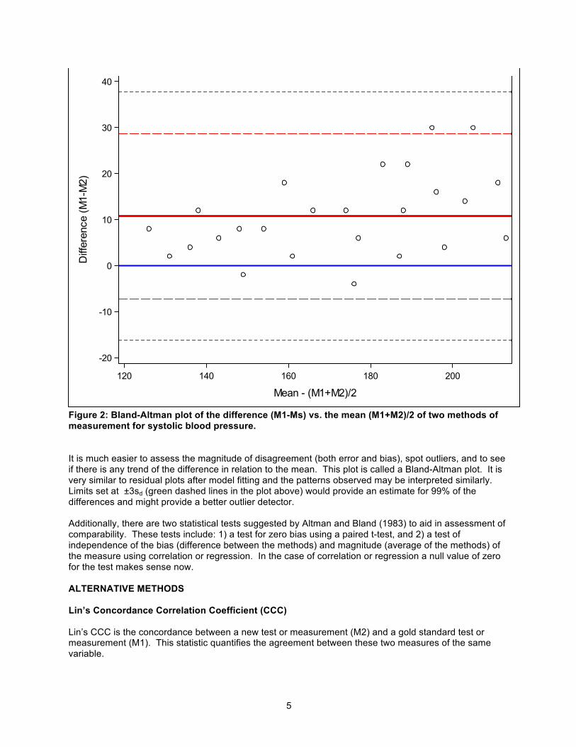
Figure 1: Scatter plot of systolic blood pressure measured using two different methods. This type of plot is familiar and is helpful for an initial look at the data but it is not the best way of looking at this type of data. The greater the range of the data the better the agreement will appear to be. A better visualization is to plot the difference between the methods (M1 – M2) against the average (M1 + M2)/2 with the addition of a horizontal line at M1-M2=0 (solid blue line), the mean of the difference (M1-M2) (solid red line), and dotted lines at ±2sd (Figure 2). The 2 standard deviation limits (dashed red lines) provide an estimate of where 95% of the differences should lie if the differences are normally distributed. The differences are likely to follow a Normal distribution because much of the variance between subjects has been removed such that measurement error is left. Plotting the horizontal line at (M1-M2)=0 and comparing the location of the horizontal line at the mean of the difference (M1-M2) aids in determining bias in one direction or another. If the horizontal line at the mean of the difference (M1-M2) is above the (M1-M2)=0 line then this is an indication that M1 measures are, on average, higher than M2 measures. Likewise, if the horizontal line at the mean of the difference (M1-M2) is below the (M1-M2)=0 line then this is an indication that M1 measures are, on average, lower than M2 measures.

125 150 175 200 225

Method 1

125

150

175

200

225

Met

hod

2

5

Figure 2: Bland-Altman plot of the difference (M1-Ms) vs. the mean (M1+M2)/2 of two methods of measurement for systolic blood pressure. It is much easier to assess the magnitude of disagreement (both error and bias), spot outliers, and to see if there is any trend of the difference in relation to the mean. This plot is called a Bland-Altman plot. It is very similar to residual plots after model fitting and the patterns observed may be interpreted similarly. Limits set at ±3sd (green dashed lines in the plot above) would provide an estimate for 99% of the differences and might provide a better outlier detector. Additionally, there are two statistical tests suggested by Altman and Bland (1983) to aid in assessment of comparability. These tests include: 1) a test for zero bias using a paired t-test, and 2) a test of independence of the bias (difference between the methods) and magnitude (average of the methods) of the measure using correlation or regression. In the case of correlation or regression a null value of zero for the test makes sense now. ALTERNATIVE METHODS Lin’s Concordance Correlation Coefficient (CCC) Lin’s CCC is the concordance between a new test or measurement (M2) and a gold standard test or measurement (M1). This statistic quantifies the agreement between these two measures of the same variable.

120 140 160 180 200

Mean - (M1+M2)/2

-20

-10

0

10

20

30

40D

iffer

ence

(M1-

M2)

6

Like correlation, the CCC ranges from -1 to 1, with perfect agreement at 1. It cannot exceed the absolute value of the correlation between M1 and M2. It can be legitimately calculated on as few as ten observations. The results have been shown to be very similar to intraclass correlation. It represents an assessment of agreement between alternative methods for continuous data that appears to avoid all the shortcomings associated with the usual procedures (Pearson correlation coefficient r, paired t-tests, least squares analysis for slope and intercept). It gives one statistic to quantify the agreement that but it might not quantify systematic bias which can be easily visualized using a Bland-Altman plot. SAS does not yet implement a calculation for this statistic. An example of SAS code can be found at https://onlinecourses.science.psu.edu/stat509/node/161. Kendall’s Tau-b Correlation Coefficient Kendall’s tau-b is a nonparametric measure of association based on the number of concordances and discordances in paired observations. Concordance occurs when paired observations vary together, and discordance occurs when paired observations vary differently. SAS® PROC CORR computes Kendall’s tau-b by ranking data. The data are double sorted by ranking observations according to values of the first variable (M1) and re-ranking the observations according to the values of the second variable (M2). Kendall’s tau-b is computed from the number of interchanges of M1 and corrects for tied pairs (pairs of observations with equal rankings of M1 or M2). Like correlation Kendall’s tau-b provides a measure of association and not agreement so it will not help to answer the question of comparability. EXAMPLE Systolic Blood Pressure: Descriptive statistics (Output 1) for the systolic blood pressure of each measurement method were determined using SAS® STAT/PROC MEANS and are below.

Variable N Mean Std Dev Lower 95% CL for Mean

Upper 95% CL for Mean

m1 m2 diffm1m2 meanm1m2

25 25 25 25

177.6000000 166.8800000 10.7200000 172.2400000

28.7691965 24.7728346 8.9792353 26.4674013

165.7246593 156.6542765 7.0135538 161.3147937

189.4753407 177.1057235 14.4264462 183.1652063

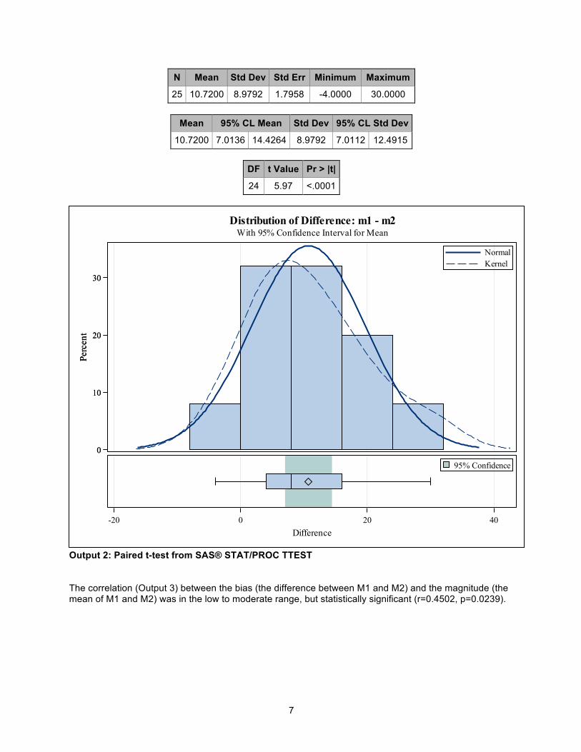
Output 1: Descriptive statistics from SAS® STAT/PROC MEANS Figure 1 provides a scatter plot of Method 2 vs. Method 1 for the systolic blood pressure example. From this plot it appears that average systolic blood pressure are measured higher using method 1 compared to method 2 in the upper portion of the plot. Examining the Bland-Altman plot in Figure 2 we see that there is an increase in bias (the difference: M1-M2) as the magnitude of the measurement increases (the mean: (M1+M2)/2)). Additionally, the mean of the differences (the solid red line) is above the 0 reference line (solid blue line) indicating that measurements from method 1 tends to be higher, on average, compared to method 2. The test for zero bias using a paired t-test (Output 2) was statistically significant (t(24)=5.97, p<0.0001) indicating that there is bias between the methods with method 1 having higher systolic blood pressure measures than method 2, on average.

7

N Mean Std Dev Std Err Minimum Maximum

25 10.7200 8.9792 1.7958 -4.0000 30.0000

Mean 95% CL Mean Std Dev 95% CL Std Dev

10.7200 7.0136 14.4264 8.9792 7.0112 12.4915

DF t Value Pr > |t|

24 5.97 <.0001

Output 2: Paired t-test from SAS® STAT/PROC TTEST The correlation (Output 3) between the bias (the difference between M1 and M2) and the magnitude (the mean of M1 and M2) was in the low to moderate range, but statistically significant (r=0.4502, p=0.0239).

With 95% Confidence Interval for MeanDistribution of Difference: m1 - m2

95% Confidence

0

10

20

30

Perc

ent

0

10

20

30

Perc

ent

KernelNormal

-20 0 20 40Difference

8

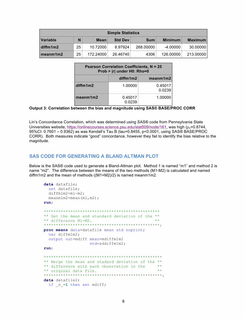
Simple Statistics

Variable N Mean Std Dev Sum Minimum Maximum

diffm1m2 25 10.72000 8.97924 268.00000 -4.00000 30.00000

meanm1m2 25 172.24000 26.46740 4306 126.00000 213.00000

Pearson Correlation Coefficients, N = 25 Prob > |r| under H0: Rho=0

diffm1m2 meanm1m2

diffm1m2 1.00000

0.45017 0.0239

meanm1m2 0.45017 0.0239

1.00000

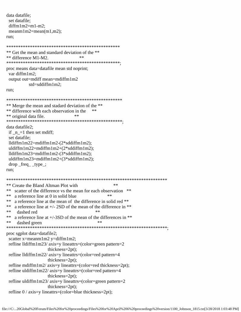
Output 3: Correlation between the bias and magnitude using SAS® BASE/PROC CORR Lin’s Concordance Correlation, which was determined using SAS® code from Pennsylvania State Universities website, https://onlinecourses.science.psu.edu/stat509/node/161, was high (ρc=0.8744, 95%CI: 0.7601 – 0.9362) as was Kendall’s Tau B (tau=0.8455, p<0.0001, using SAS® BASE/PROC CORR). Both measures indicate “good” concordance, however they fail to identify the bias relative to the magnitude. SAS CODE FOR GENERATING A BLAND ALTMAN PLOT Below is the SAS® code used to generate a Bland-Altman plot. Method 1 is named “m1” and method 2 is name “m2”. The difference between the means of the two methods (M1-M2) is calculated and named diffm1m2 and the mean of methods ((M1+M2)/2) is named meanm1m2.

data datafile; set datafile; diffm1m2=m1-m2; meanm1m2=mean(m1,m2); run;

************************************************ ** Get the mean and standard deviation of the ** ** difference M1-M2. ** ************************************************; proc means data=datafile mean std noprint; var diffm1m2; output out=mdiff mean=mdiffm1m2 std=sddiffm1m2; run;

************************************************* ** Merge the mean and stadard deviation of the ** ** difference with each observation in the ** ** original data file. ** *************************************************; data datafile2; if _n_=1 then set mdiff;

9

set datafile; lldiffm1m22=mdiffm1m2-(2*sddiffm1m2); uldiffm1m22=mdiffm1m2+(2*sddiffm1m2); lldiffm1m23=mdiffm1m2-(3*sddiffm1m2); uldiffm1m23=mdiffm1m2+(3*sddiffm1m2); drop _freq_ _type_; run; ******************************************************************** ** Create the Bland Altman Plot with ** ** scatter of the difference vs the mean for each observation ** ** a reference line at 0 in solid blue ** ** a reference line at the mean of the difference in solid red ** ** a reference line at +/- 2SD of the mean of the difference in ** ** dashed red ** ** a reference line at +/-3SD of the mean of the differences in ** ** dashed green ** ********************************************************************; proc sgplot data=datafile2; scatter x=meanm1m2 y=diffm1m2; refline lldiffm1m23/ axis=y lineattrs=(color=green pattern=2 thickness=2pt); refline lldiffm1m22/ axis=y lineattrs=(color=red pattern=4 thickness=2pt); refline mdiffm1m2/ axis=y lineattrs=(color=red thickness=2pt); refline uldiffm1m22/ axis=y lineattrs=(color=red pattern=4 thickness=2pt); refline uldiffm1m23/ axis=y lineattrs=(color=green pattern=2 thickness=2pt); refline 0 / axis=y lineattrs=(color=blue thickness=2pt); yaxis label='Difference (M1-M2)'; xaxis label='Mean - (M1+M2)/2'; title 'Bland-Altman Plot of Difference (M1-M2) vs Mean'; run;

CONCLUSIONS As a statistician, it is important to understand that agreement does not equal comparability and to understand what the inferential statistical methods applied are testing. Linear regression, t-tests, and Pearson Product Moment correlation are not appropriate measures to examining comparability of two methods of measurement as they are testing something else. Altman and Bland (1983) proposed using a visual method for examining comparability that plots the bias (difference between the two methods) versus the magnitude (mean of the two methods) to look at comparability and assess for any potential patterns (e.g. increasing bias with increasing magnitude). Additionally, Altman and Bland (1983) proposed using a paired t-test to test for zero bias between the methods and a Pearson Product Moment correlation coefficient as a test of independence between the bias and magnitude. REFERENCES

1. Altman DG, Bland JM. Measurement in medicine: the analysis of method comparison studies. The Statistician 32 (1983), 307-317.

2. Lin LI. A concordance correlation coefficient to evaluate reproducibility. Biometrics 45 (1989), 255-268.

10

3. Rohatgi, A. 2017. “WebPlotDigitizer”. Accessed July 26, 2017. https://automeris.io/WebPlotDigitizer/

4. Sharp King T, Lengerich R, Bai S. “Lesson 18: Correlation and Agreement. 18.6 – Concordance Correlation for Measuring Agreement”. Accessed March 4, 2018. https://onlinecourses.science.psu.edu/stat509/node/161

CONTACT INFORMATION Maribeth Johnson majohnso@augusta.edu Jennifer Waller jwaller@augusta.edu SAS and all other SAS Institute Inc. product or service names are registered trademarks or trademarks of SAS Institute Inc. in the USA and other countries. ® indicates USA registration.

Other brand and product names are trademarks of their respective companies.

file:///C/...20Global%20Forum/Files%20for%20proceedings/Files%20for%20April%206%20proceedings%20version/1100_Johnson_1815.txt[3/28/2018 1:03:48 PM]

data datafile; set datafile; diffm1m2=m1-m2; meanm1m2=mean(m1,m2);run;

************************************************** Get the mean and standard deviation of the **** difference M1-M2. **************************************************;proc means data=datafile mean std noprint; var diffm1m2; output out=mdiff mean=mdiffm1m2 std=sddiffm1m2;run;

*************************************************** Merge the mean and stadard deviation of the **** difference with each observation in the **** original data file. ***************************************************;data datafile2; if _n_=1 then set mdiff; set datafile; lldiffm1m22=mdiffm1m2-(2*sddiffm1m2); uldiffm1m22=mdiffm1m2+(2*sddiffm1m2); lldiffm1m23=mdiffm1m2-(3*sddiffm1m2); uldiffm1m23=mdiffm1m2+(3*sddiffm1m2); drop _freq_ _type_;run;

********************************************************************** Create the Bland Altman Plot with **** scatter of the difference vs the mean for each observation **** a reference line at 0 in solid blue **** a reference line at the mean of the difference in solid red **** a reference line at +/- 2SD of the mean of the difference in **** dashed red **** a reference line at +/-3SD of the mean of the differences in **** dashed green **********************************************************************;proc sgplot data=datafile2; scatter x=meanm1m2 y=diffm1m2; refline lldiffm1m23/ axis=y lineattrs=(color=green pattern=2 thickness=2pt); refline lldiffm1m22/ axis=y lineattrs=(color=red pattern=4 thickness=2pt); refline mdiffm1m2/ axis=y lineattrs=(color=red thickness=2pt); refline uldiffm1m22/ axis=y lineattrs=(color=red pattern=4 thickness=2pt); refline uldiffm1m23/ axis=y lineattrs=(color=green pattern=2 thickness=2pt); refline 0 / axis=y lineattrs=(color=blue thickness=2pt);

file:///C/...20Global%20Forum/Files%20for%20proceedings/Files%20for%20April%206%20proceedings%20version/1100_Johnson_1815.txt[3/28/2018 1:03:48 PM]

yaxis label='Difference (M1-M2)'; xaxis label='Mean - (M1+M2)/2';title 'Bland-Altman Plot of Difference (M1-M2) vs Mean';run;