Simple Regression Department of Applied Economics National Chung Hsing University

Simple Regression

Department of Applied Economics

National Chung Hsing University

Linear Functions

• Formula: Y = a + bX– Is a linear formula. If you graphed X and Y for any

chosen values of a and b, you’d get a straight line.– It is a family of functions: For any value of a and b,

you get a particular line

• a is referred to as the “constant” or “intercept”

• b is referred to as the “slope”

• To graph a linear function: Pick values for X, compute corresponding values of Y

• Then, connect dots to graph line

Linear Functions: Y = a + bX

Y axis

X axis

-10 -5 0 5 10

20

10

-10

-20

• The “constant” or “intercept” (a)– Determines where the line intersects the Y-axis– If a increases (decreases), the line moves up (down)

Y= 3 -1.5X

Y= -9 - 1.5X

Y=14 - 1.5X

Linear Functions: Y = a + bX

• The slope (b) determines the steepness of the line

Y axis

X axis

-10 -5 0 5 10

20

10

-10

-20

Y=3-1.5X

Y=3+.2X

Y=3+3X

Linear Functions: Slopes

• The slope (b) is the ratio of change in Y to change in X

-10 -5 0 5 10

20

10

-10

-20Y=3+3X

The slope tells you howmany points Y will

increase for any singlepoint increase in X

Change in X =5

Change in Y=15

Slope:

b = 15/5 = 3

INCOME

100000800006000040000200000

HA

PP

Y

10

9

8

7

6

5

4

3

2

1

0

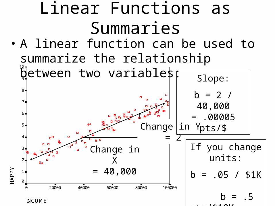
Linear Functions as Summaries

• A linear function can be used to summarize the relationship between two variables:

Change in X= 40,000

Change in Y = 2

Slope:

b = 2 / 40,000 = .00005 pts/$

If you change units:

b = .05 / $1K b = .5 pts/$10K b = 5 pts/$100K

INCOME

100000800006000040000200000

HA

PP

Y

10

9

8

7

6

5

4

3

2

1

0


• Slope and constant can be “eyeballed” to approximate a formula:

Slope (b):

b = 2 / 40,000 = .00005 pts/$

Constant (a) = Value where line

hits Y axis

a = 2

Happy = 2 + .00005Income

Linear Functions as Summaries• Linear functions can powerfully summarize data:

– Formula: Happy = 2 + .00005Income

• Gives a sense of how the two variables are related– Namely, people get a .00005 increase in happiness for

every extra dollar of income (or 5 pts per $100K)

• Also lets you “predict” values. What if someone earns $150,000? – Happy = 2 + .00005($150,000) = 9.5

• But be careful… You shouldn’t assume that a relationship remains linear indefinitely– Also, negative income or happiness make no sense…

EDUCATN

20181614121086420

PR

ES

TIG

E

100

90

80

70

60

50

40

30

20

10

0

-10

-20

-30

-40


• Come up with a linear function that summarizes this real data: years of education vs. job prestige

It isn’t always easy! The line you choose

depends on how much you “weight” these

points.

Computing Regressions

• Regression coefficients can be calculated in SPSS– You will rarely, if ever, do them by hand

• SPSS will estimate:– The value of the constant (a)– The value of the slope (b)– Plus, a large number of related statistics and results of

hypothesis testing procedures

EDUCATN

20181614121086420

PR

ES

TIG

E

100

90

80

70

60

50

40

30

20

10

0

-10

-20

-30

-40

Example: Education & Job Prestige

• Example: Years of Education versus Job Prestige– Previously, we made an “eyeball” estimate of the line

Our estimate:

Y = 5 + 3X

Model Summary

.521a .272 .271 12.40Model1

R R SquareAdjustedR Square

Std. Error ofthe Estimate

Predictors: (Constant), HIGHEST YEAR OF SCHOOLCOMPLETED

a.


• The actual SPSS regression results for that data:

Coefficientsa

9.427 1.418 6.648 .000

2.487 .108 .521 23.102 .000

(Constant)

HIGHEST YEAR OFSCHOOL COMPLETED

Model1

B Std. Error

UnstandardizedCoefficients

Beta

Standardized

Coefficients

t Sig.

Dependent Variable: RS OCCUPATIONAL PRESTIGE SCOREa.

Estimates of a and b: “Constant” = a = 9.427

Slope for “Year of School” = b = 2.487

• Equation: Prestige = 9.4 + 2.5 Education

• A year of education adds 2.5 points job prestige

EDUCATN

20181614121086420

PR

ES

TIG

E

100

90

80

70

60

50

40

30

20

10

0

-10

-20

-30

-40


• Comparing our “eyeball” estimate to the actual OLS regression line

Our estimate:

Y = 5 + 3X

Actual OLS regression line computed in

SPSS

R-Square

• The R-Square statistic indicates how well the regression line “explains” variation in Y

• It is based on partitioning variance into:

• 1. Explained (“regression”) variance– The portion of deviation from Y-bar accounted for by

the regression line

• 2. Unexplained (“error”) variance– The portion of deviation from Y-bar that is “error”

• Formula:22

22

YX

YX

TOTAL

REGRESSIONYX ss

s

SS

SSR

R-Square

• Visually: Deviation is partitioned into two parts

-4 -2 0 2 4

4

2

-2

-4

Y-bar

“Explained Variance”

Y=2+.5X

“Error Variance”


• R-Square & Hypothesis testing information:Model Summary

.521a .272 .271 12.40Model1




a.

Coefficientsa

9.427 1.418 6.648 .000

2.487 .108 .521 23.102 .000

(Constant)


Model1

B Std. Error


Beta

Standardized

Coefficients

t Sig.


This information allows us to do hypothesis tests about constant & slope

The R and R-Square indicate how well the line

summarizes the data

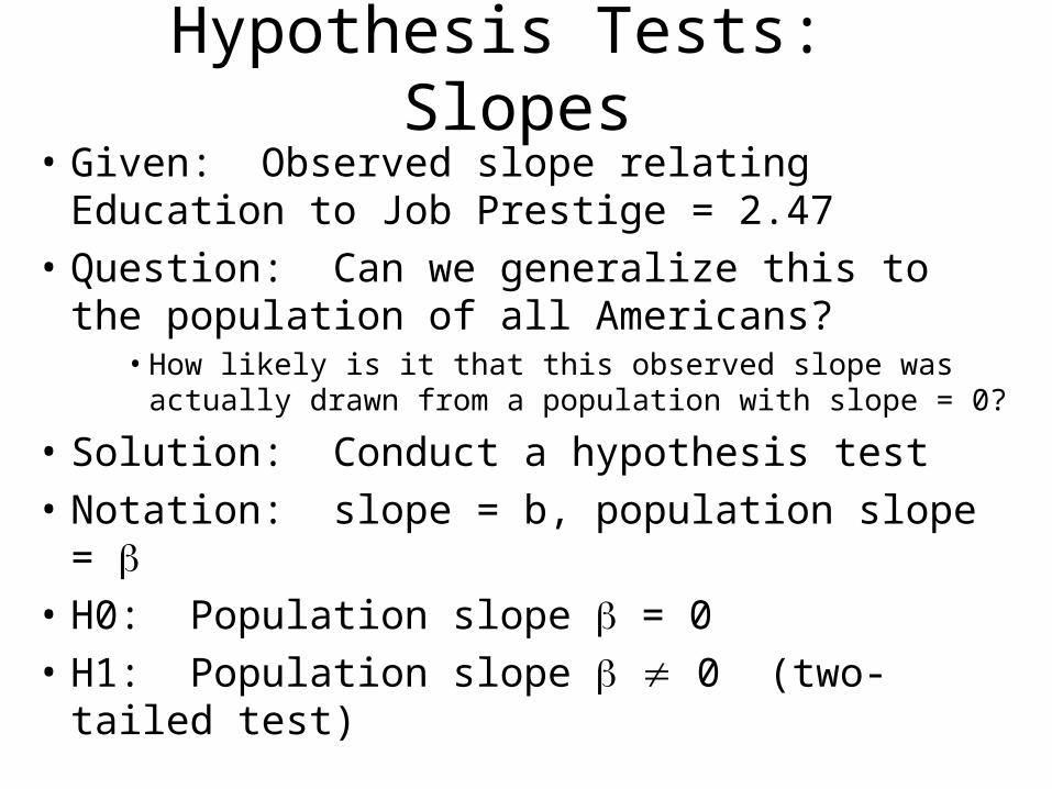
Hypothesis Tests: Slopes

• Given: Observed slope relating Education to Job Prestige = 2.47

• Question: Can we generalize this to the population of all Americans?

• How likely is it that this observed slope was actually drawn from a population with slope = 0?

• Solution: Conduct a hypothesis test

• Notation: slope = b, population slope = • H0: Population slope = 0

• H1: Population slope 0 (two-tailed test)

Model Summary

.521a .272 .271 12.40Model1




a.

Example: Slope Hypothesis Test

• The actual SPSS regression results for that data:

Coefficientsa

9.427 1.418 6.648 .000

2.487 .108 .521 23.102 .000

(Constant)


Model1

B Std. Error


Beta

Standardized

Coefficients

t Sig.


t-value and “sig” (p-value) are for hypothesis

tests about the slope

• Reject H0 if: T-value > critical t (N-2 df)

• Or, “sig.” (p-value) less than often =


• What information lets us to do a hypothesis test?

• Answer: Estimates of a slope (b) have a sampling distribution, like any other statistic– It is the distribution of every value of the slope, based

on all possible samples (of size N)

• If certain assumptions are met, the sampling distribution approximates the t-distribution– Thus, we can assess the probability that a given value

of b would be observed, if = 0– If probability is low – below alpha – we reject H0

0

Sampling distribution of

the slope


• Visually: If the population slope () is zero, then the sampling distribution would center at zero– Since the sampling distribution is a probability

distribution, we can identify the likely values of b if the population slope is zero

If =0, observed slopes should commonly fall near zero, too

b

If observed slope falls very far from 0, it is improbable that is really equal to zero. Thus, we

can reject H0.

Regression Assumptions• Assumptions of simple (bivariate) regression

• If assumptions aren’t met, hypothesis tests may be inaccurate

– 1. Random sample w/ sufficient N (N > ~20)– 2. Linear relationship among variables

• Check scatterplot for non-linear pattern; (a “cloud” is OK)

– 3. Conditional normality: Y = normal at all values of X• Check histograms of Y for normality at several values of X

– 4. Homoskedasticity – equal error variance at all values of X

• Check scatterplot for “bulges” or “fanning out” of error across values of X

– Additional assumptions are required for multivariate regression…

Bivariate Regression Assumptions

• Normality:

INCOME

100000800006000040000200000

HA

PP

Y

10

8

6

4

2

0

Examine sub-samples at different values of X. Make histograms and check for normality.

HAPPY

8.00

7.50

7.00

6.50

6.00

5.50

5.00

4.50

4.00

3.50

3.00

2.50

2.00

1.50

1.00

.50

12

10

8

6

4

2

0

Std. Dev = 1.51

Mean = 3.84

N = 60.00

Good

HAPPY

10.00

9.50

9.00

8.50

8.00

7.50

7.00

6.50

6.00

5.50

5.00

4.50

4.00

3.50

3.00

2.50

2.00

1.50

1.00

.50

12

10

8

6

4

2

0

Std. Dev = 3.06

Mean = 4.58

N = 60.00

Not very good

INCOME

100000800006000040000200000

HA

PP

Y

10

8

6

4

2

0


• Homoskedasticity: Equal Error Variance

Examine error at different values of X.

Is it roughly equal?

Here, things look pretty good.

INCOME

100000

90000

80000

70000

60000

50000

40000

30000

20000

10000

0

HA

PP

Y

10

8

6

4

2

0


• Heteroskedasticity: Unequal Error Variance

At higher values of X, error variance increases a lot.

This looks pretty bad.

Regression Hypothesis Tests

• If assumptions are met, the sampling distribution of the slope (b) approximates a T-distribution

• Standard deviation of the sampling distribution is called the standard error of the slope (b)

• Population formula of standard error:

N

ii

eb

XX1

2

2

)(

• Where e2 is the variance of the regression error

Regression Hypothesis Tests

• Finally: A t-value can be calculated:• It is the slope divided by the standard error

)1(2

2

Ns

MS

b

s

bt

X

ERROR

YX

b

YXN

• Where sb is the sample point estimate of the S.E.

• The t-value is based on N-2 degrees of freedom

• Reject H0 if observed t > critical t (e.g., 1.96).

Coefficientsa

9.427 1.418 6.648 .000

2.487 .108 .521 23.102 .000

(Constant)


Model1

B Std. Error


Beta

Standardized

Coefficients

t Sig.



• T-values can be compared to critical t...

SPSS estimates the standard error of the slope. This is used to calculate

a t-value

The t-value can be compared to the “critical value” to test hypotheses. Or,

just compare “Sig.” to alpha.

If t > crit or Sig < alpha, reject H0

Multiple Regression 1

Department of Applied Economics

National Chung Hsing University

Multiple Regression

• Question: What if a dependent variable is affected by more than one independent variable?

• Strategy #1: Do separate bivariate regressions– One regression for each independent variable

• This yields separate slope estimates for each independent variable– Bivariate slope estimates implicitly assume that

neither independent variable mediates the other– In reality, there might be no effect of family wealth

over and above education

Multiple Regression

Coefficientsa

35.608 1.290 27.611 .000

2.075 .446 .122 4.652 .000

(Constant)

RS FAMILY INCOMEWHEN 16 YRS OLD

Model1

B Std. Error


Beta

Standardized

Coefficients

t Sig.

Dependent Variable: RS OCCUPATIONAL PRESTIGE SCORE (1970)a.

Coefficientsa

9.417 1.421 6.625 .000

2.488 .108 .520 23.056 .000

(Constant)


Model1

B Std. Error


Beta

Standardized

Coefficients

t Sig.


• Job Prestige: Two separate regression models

Both variables have positive, significant slopes

Multiple Regression

• Idea #2: Use Multiple Regression

• Multiple regression can examine “partial” relationships– Partial = Relationships after the effects of other

variables have been “controlled” (taken into account)

• This lets you determine the effects of variables “over and above” other variables– And shows the relative impact of different factors on

a dependent variable

• And, you can use several independent variables to improve your predictions of the dependent var

Coefficientsa

8.977 1.629 5.512 .000

2.487 .111 .520 22.403 .000

.178 .394 .011 .453 .651

(Constant)



Model1

B Std. Error


Beta

Standardized

Coefficients

t Sig.


Multiple Regression

• Job Prestige: 2 variable multiple regression

Education slope is basically unchanged

Family Income slope decreases compared to bivariate analysis

(bivariate: b = 2.07) And, outcome of hypothesis

test changes – t < 1.96

Multiple Regression• Ex: Job Prestige: 2 variable multiple regression• 1. Education has a large slope effect controlling

for (i.e. “over and above”) family income• 2. Family income does not have much effect

controlling for education• Despite a strong bivariate relationship

• Possible interpretations: • Family income may lead to education, but education is the

critical predictor of job prestige• Or, family income is wholly unrelated to job prestige… but

is coincidentally correlated with a variable that is (education), which generated a spurious “effect”.

The Multiple Regression Model

• A two-independent variable regression model:

iiii eXbXbaY 2211

• Note: There are now two X variables

• And a slope (b) is estimated for each one

• The full multiple regression model is:

ikikiii eXbXbXbaY 2211

• For k independent variables

Multiple Regression: Slopes

• Regression slope for the two variable case:

21

21

2121

11 XX

XXYXYX

X

Y

r

rrr

s

sb

• b1 = slope for X1 – controlling for the other independent variable X2

• b2 is computed symmetrically. Swap X1s, X2s

• Compare to bivariate slope: YXX

YYX r

s

sb

Multiple Regression Slopes

• Let’s look more closely at the formulas:

21

21

2121

11 XX

XXYXYX

X

Y

r

rrr

s

sb

• What happens to b1 if X1 and X2 are totally uncorrelated?

• Answer: The formula reduces to the bivariate

• What if X1 and X2 are correlated with each other AND X2 is more correlated with Y than X1?

• Answer: b1 gets smaller (compared to bivariate)

YXX

YYX r

s

sbversus

Regression Slopes

• So, if two variables (X1, X2) are correlated and both predict Y:

• The X variable that is more correlated with Y will have a higher slope in multivariate regression– The slope of the less-correlated variable will shrink

• Thus, slopes for each variable are adjusted to how well the other variable predicts Y– It is the slope “controlling” for other variables.

Multiple Regression Slopes

• One last thing to keep in mind…

21

21

2121

11 XX

XXYXYX

X

Y

r

rrr

s

sb

• What happens to b1 if X1 and X2 are almost perfectly correlated?

• Answer: The denominator approaches Zero

• The slope “blows up”, approaching infinity

• Highly correlated independent variables can cause trouble for regression models… watch out

YXX

YYX r

s

sbversus

Interpreting Results

• (Over)Simplified rules for interpretation– Assumes good sample, measures, models, etc.

• Multivariate regression with two variables: A, B

• If slopes of A, B are the same as bivariate, then each has an independent effect

• If A remains large, B shrinks to zero we typically conclude that effect of B was spurious, or operates through A

• If both A and B shrink a little, each has an effect, but some overlap or mediation is occurring

Interpreting Multivariate Results

• Things to watch out for:

• 1. Remember: Correlation is not causation– Ability to “control” for many variables can help detect

spurious relationships… but it isn’t perfect.– Be aware that other (omitted) variables may be

affecting your model. Don’t over-interpret results.

• 2. Reverse causality– Many sociological processes involve bi-directional

causality. Regression slopes (and correlations) do not identify which variable “causes” the other.

• Ex: self-esteem and test scores.

Standardized Regression Coefficients

• Regression slopes reflect the units of the independent variables

• Question: How do you compare how “strong” the effects of two variables if they have totally different units?

• Example: Education, family wealth, job prestige– Education measured in years, b = 2.5– Family wealth measured on 1-5 scale, b = .18– Which is a “bigger” effect? Units aren’t comparable!

• Answer: Create “standardized” coefficients


• Standardized Coefficients– Also called “Betas” or Beta Weights”– Symbol: Greek b with asterisk: * – Equivalent to Z-scoring (standardizing) all

independent variables before doing the regression

• Formula of coeficient for Xj:j

Y

X

j bs

sj

*

• Result: The unit is standard deviations

• Betas: Indicates the effect a 1 standard deviation change in Xj on Y


• Ex: Education, family income, and job prestige:Coefficientsa

8.977 1.629 5.512 .000

2.487 .111 .520 22.403 .000

.178 .394 .011 .453 .651

(Constant)



Model1

B Std. Error


Beta

Standardized

Coefficients

t Sig.


An increase of 1 standard deviation in Education results

in a .52 standard deviation increase in job prestige Betas give you a sense of

which variables “matter most”

What is the interpretation of the “family income” beta?

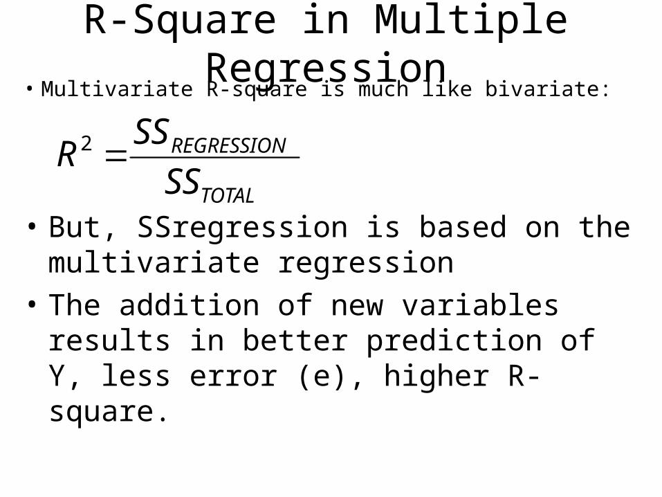
R-Square in Multiple Regression• Multivariate R-square is much like bivariate:

TOTAL

REGRESSION

SS

SSR 2

• But, SSregression is based on the multivariate regression

• The addition of new variables results in better prediction of Y, less error (e), higher R-square.

Model Summary

.522a .272 .271 12.41Model1



Predictors: (Constant), INCOM16, EDUCa.

R-Square in Multiple Regression• Example:

• R-square of .272 indicates that education, parents wealth explain 27% of variance in job prestige

• “Adjusted R-square” is a more conservative, more accurate measure in multiple regression– Generally, you should report Adjusted R-square.

Dummy Variables

• Question: How can we incorporate nominal variables (e.g., race, gender) into regression?

• Option 1: Analyze each sub-group separately– Generates different slope, constant for each group

• Option 2: Dummy variables– “Dummy” = a dichotomous variables coded to

indicate the presence or absence of something– Absence coded as zero, presence coded as 1.

Dummy Variables

• Strategy: Create a separate dummy variable for all nominal categories

• Ex: Gender – make female & male variables– DFEMALE: coded as 1 for all women, zero for men– DMALE: coded as 1 for all men

• Next: Include all but one dummy variables into a multiple regression model

• If two dummies, include 1; If 5 dummies, include 4.

Dummy Variables

• Question: Why can’t you include DFEMALE and DMALE in the same regression model?

• Answer: They are perfectly correlated (negatively): r = -1– Result: Regression model “blows up”

• For any set of nominal categories, a full set of dummies contains redundant information– DMALE and DFEMALE contain same information– Dropping one removes redundant information.

Dummy Variables: Interpretation

• Consider the following regression equation:

iiii eDFEMALEbINCOMEbaY 21

• Question: What if the case is a male?

• Answer: DFEMALE is 0, so the entire term becomes zero.– Result: Males are modeled using the familiar

regression model: a + b1X + e.


• Consider the following regression equation:

iiii eDFEMALEbINCOMEbaY 21

• Question: What if the case is a female?

• Answer: DFEMALE is 1, so b2(1) stays in the equation (and is added to the constant)– Result: Females are modeled using a different

regression line: (a+b2) + b1X + e

– Thus, the coefficient of b2 reflects difference in the constant for women.


• Remember, a different constant generates a different line, either higher or lower– Variable: DFEMALE (women = 1, men = 0)– A positive coefficient (b) indicates that women are

consistently higher compared to men (on dep. var.)– A negative coefficient indicated women are lower

• Example: If DFEMALE coeff = 1.2:– “Women are on average 1.2 points higher than men”.

Dummy Variables: Interpretation• Visually: Women = blue, Men = red

INCOME

100000800006000040000200000

HA

PP

Y

10

9

8

7

6

5

4

3

2

1

0

Overall slope for all data points

Note: Line for men, women have same slope… but one is

high other is lower. The constant differs!

If women=1, men=0: The constant (a) reflects

men only. Dummy coefficient (b) reflects

increase for women (relative to men)

Dummy Variables

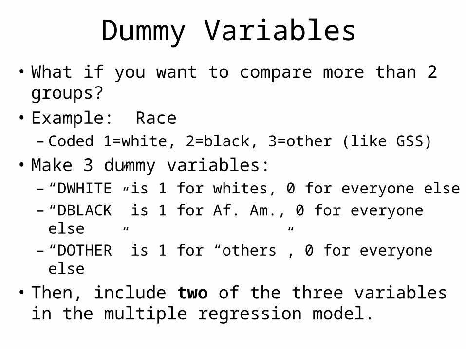
• What if you want to compare more than 2 groups?

• Example: Race– Coded 1=white, 2=black, 3=other (like GSS)

• Make 3 dummy variables:– “DWHITE” is 1 for whites, 0 for everyone else– “DBLACK” is 1 for Af. Am., 0 for everyone else– “DOTHER” is 1 for “others”, 0 for everyone else

• Then, include two of the three variables in the multiple regression model.

Coefficientsa

9.666 1.672 5.780 .000

2.476 .111 .517 22.271 .000

6.282E-02 .397 .004 .158 .874

-2.666 1.117 -.055 -2.388 .017

1.114 1.777 .014 .627 .531

(Constant)

EDUC

INCOM16

DBLACK

DOTHER

Model1

B Std. Error


Beta

Standardized

Coefficients

t Sig.

Dependent Variable: PRESTIGEa.


• Ex: Job Prestige

• Negative coefficient for DBLACK indicates a lower level of job prestige compared to whites– T- and P-values indicate if difference is significant.


• Comments:

• 1. Dummy coefficients shouldn’t be called slopes– Referring to the “slope” of gender doesn’t make sense– Rather, it is the difference in the constant (or “level”)

• 2. The contrast is always with the nominal category that was left out of the equation– If DFEMALE is included, the contrast is with males– If DBLACK, DOTHER are included, coefficients

reflect difference in constant compared to whites.

Documents

Simple Regression Department of Applied Economics National Chung Hsing University