Embed Size (px)
DESCRIPTION
Data and attributes and parameters.The data type and protocolEffectiveness of working in the environment.Research tabulation.
Citation preview

7/15/2019 Simple Tabulation 7and.ppt
http://slidepdf.com/reader/full/simple-tabulation-7andppt 1/52
Simple Tabulation
Cross Tabulation
Chi-square
7/15/2019 Simple Tabulation 7and.ppt
http://slidepdf.com/reader/full/simple-tabulation-7andppt 2/52
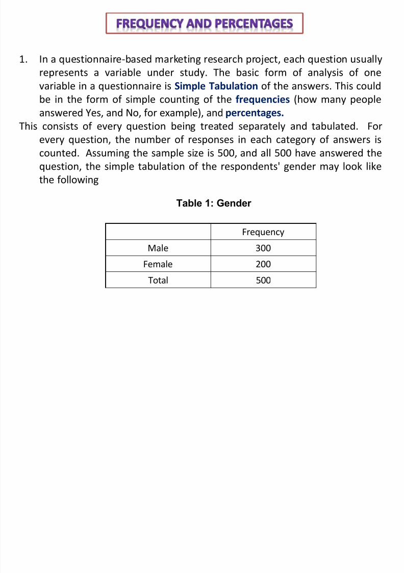
1. In a questionnaire-based marketing research project, each question usually
represents a variable under study. The basic form of analysis of onevariable in a questionnaire is Simple Tabulation of the answers. This could
be in the form of simple counting of the frequencies (how many people
answered Yes, and No, for example), and percentages.
This consists of every question being treated separately and tabulated. For
every question, the number of responses in each category of answers iscounted. Assuming the sample size is 500, and all 500 have answered the
question, the simple tabulation of the respondents' gender may look like
the following
Frequency
Male 300
Female 200
Total 500
Table 1: Gender
7/15/2019 Simple Tabulation 7and.ppt
http://slidepdf.com/reader/full/simple-tabulation-7andppt 3/52
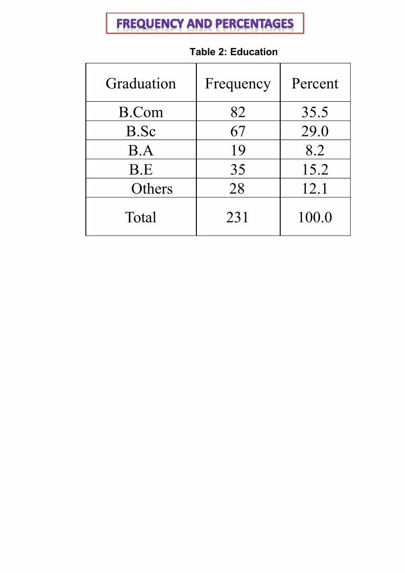
Graduation Frequency Percent
B.Com 82 35.5
B.Sc 67 29.0
B.A 19 8.2
B.E 35 15.2
Others 28 12.1
Total 231 100.0
Table 2: Education
7/15/2019 Simple Tabulation 7and.ppt
http://slidepdf.com/reader/full/simple-tabulation-7andppt 4/52
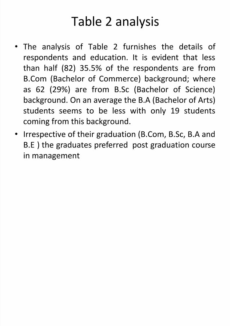
Table 2 analysis
• The analysis of Table 2 furnishes the details of
respondents and education. It is evident that less
than half (82) 35.5% of the respondents are from
B.Com (Bachelor of Commerce) background; whereas 62 (29%) are from B.Sc (Bachelor of Science)
background. On an average the B.A (Bachelor of Arts)
students seems to be less with only 19 students
coming from this background.
• Irrespective of their graduation (B.Com, B.Sc, B.A and
B.E ) the graduates preferred post graduation course
in management
7/15/2019 Simple Tabulation 7and.ppt
http://slidepdf.com/reader/full/simple-tabulation-7andppt 5/52
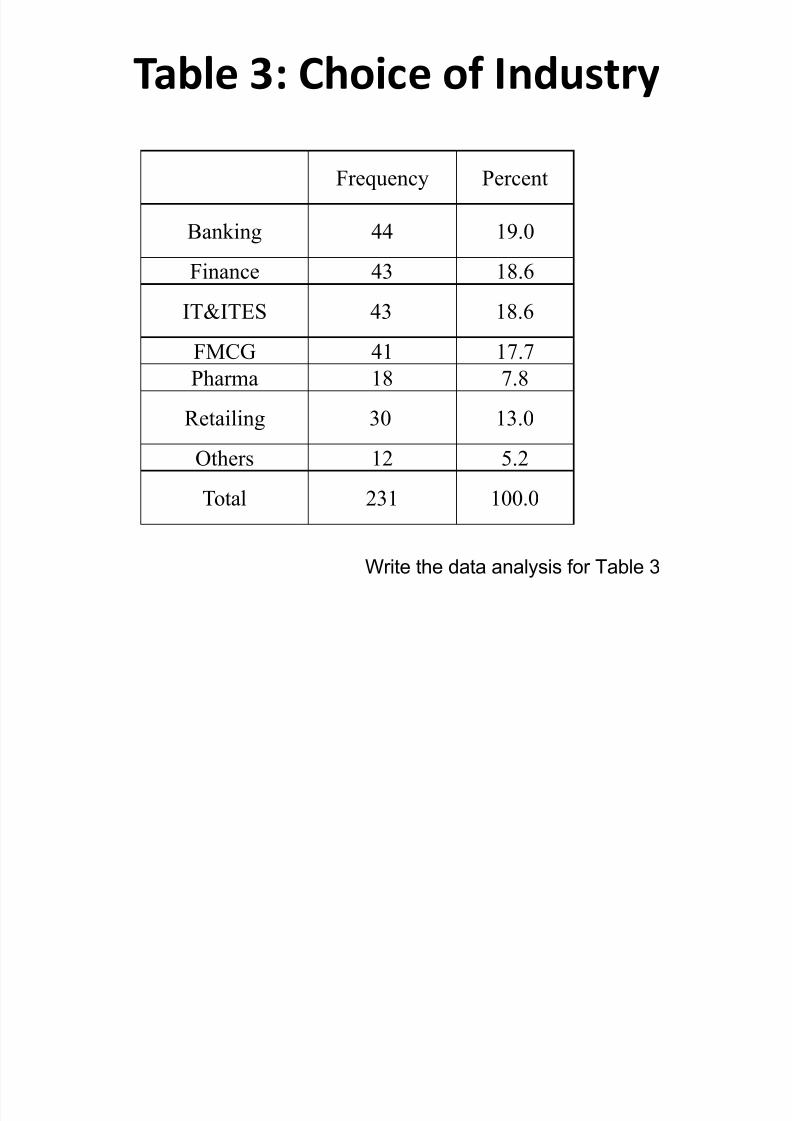
Table 3: Choice of Industry
Frequency Percent
Banking 44 19.0
Finance 43 18.6
IT&ITES 43 18.6
FMCG 41 17.7
Pharma 18 7.8
Retailing 30 13.0
Others 12 5.2
Total 231 100.0
Write the data analysis for Table 3
7/15/2019 Simple Tabulation 7and.ppt
http://slidepdf.com/reader/full/simple-tabulation-7andppt 6/52
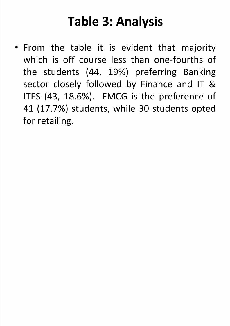
Table 3: Analysis
• From the table it is evident that majority
which is off course less than one-fourths of
the students (44, 19%) preferring Banking
sector closely followed by Finance and IT &
ITES (43, 18.6%). FMCG is the preference of
41 (17.7%) students, while 30 students opted
for retailing.
7/15/2019 Simple Tabulation 7and.ppt
http://slidepdf.com/reader/full/simple-tabulation-7andppt 7/52
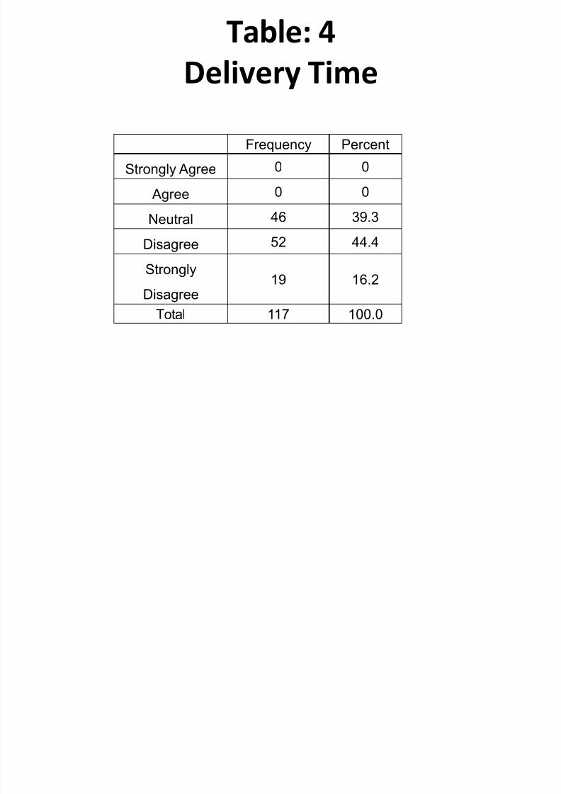
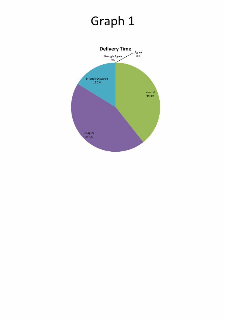
Table: 4
Delivery Time
Frequency Percent
Strongly Agree 0 0
Agree 0 0
Neutral 46 39.3
Disagree 52 44.4
Strongly
Disagree
19 16.2
Total 117 100.0
7/15/2019 Simple Tabulation 7and.ppt
http://slidepdf.com/reader/full/simple-tabulation-7andppt 8/52
Graph 1
Strongly Agree
0%
Agree
0%
Neutral
39.3%
Disagree
44.4%
Strongly Disagree16.2%
Delivery Time
7/15/2019 Simple Tabulation 7and.ppt
http://slidepdf.com/reader/full/simple-tabulation-7andppt 9/52
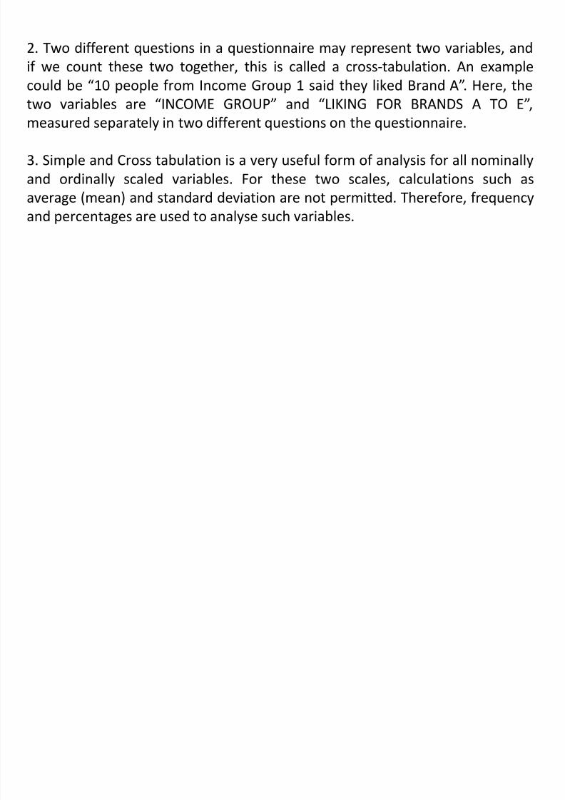
2. Two different questions in a questionnaire may represent two variables, and
if we count these two together, this is called a cross-tabulation. An example
could be “10 people from Income Group 1 said they liked Brand A”. Here, the
two variables are “INCOME GROUP” and “LIKING FOR BRANDS A TO E”, measured separately in two different questions on the questionnaire.
3. Simple and Cross tabulation is a very useful form of analysis for all nominally
and ordinally scaled variables. For these two scales, calculations such as
average (mean) and standard deviation are not permitted. Therefore, frequencyand percentages are used to analyse such variables.
7/15/2019 Simple Tabulation 7and.ppt
http://slidepdf.com/reader/full/simple-tabulation-7andppt 10/52
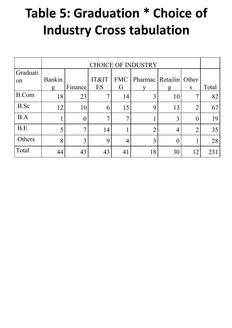
Table 5: Graduation * Choice of
Industry Cross tabulation
CHOICE OF INDUSTRY
Graduati
on Banking Finance
IT&ITES
FMCG
Pharmacy
Retailing
Other s Total
B.Com 18 23 7 14 3 10 7 82
B.Sc 12 10 6 15 9 13 2 67
B.A1 0 7 7 1 3 0 19
B.E 5 7 14 1 2 4 2 35
Others 8 3 9 4 3 0 1 28
Total 44 43 43 41 18 30 12 231
7/15/2019 Simple Tabulation 7and.ppt
http://slidepdf.com/reader/full/simple-tabulation-7andppt 11/52
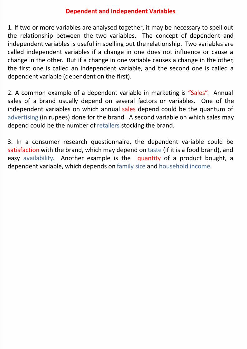
Dependent and Independent Variables
1. If two or more variables are analysed together, it may be necessary to spell out
the relationship between the two variables. The concept of dependent and
independent variables is useful in spelling out the relationship. Two variables arecalled independent variables if a change in one does not influence or cause a
change in the other. But if a change in one variable causes a change in the other,
the first one is called an independent variable, and the second one is called a
dependent variable (dependent on the first).
2. A common example of a dependent variable in marketing is “Sales”. Annual
sales of a brand usually depend on several factors or variables. One of the
independent variables on which annual sales depend could be the quantum of
advertising (in rupees) done for the brand. A second variable on which sales may
depend could be the number of retailers stocking the brand.
3. In a consumer research questionnaire, the dependent variable could be
satisfaction with the brand, which may depend on taste (if it is a food brand), and
easy availability. Another example is the quantity of a product bought, a
dependent variable, which depends on family size and household income.
7/15/2019 Simple Tabulation 7and.ppt
http://slidepdf.com/reader/full/simple-tabulation-7andppt 12/52
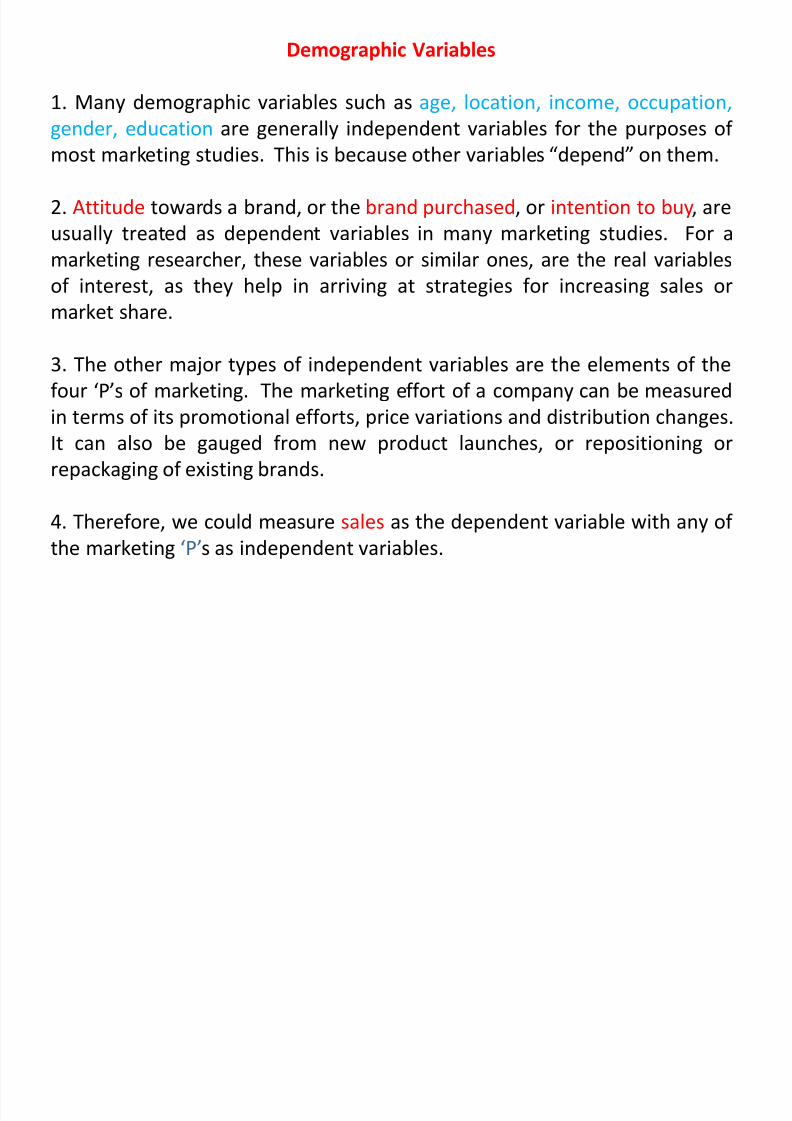
Demographic Variables
1. Many demographic variables such as age, location, income, occupation,
gender, education are generally independent variables for the purposes of
most marketing studies. This is because other variables “depend” on them.
2. Attitude towards a brand, or the brand purchased, or intention to buy, are
usually treated as dependent variables in many marketing studies. For a
marketing researcher, these variables or similar ones, are the real variables
of interest, as they help in arriving at strategies for increasing sales or
market share.
3. The other major types of independent variables are the elements of the
four ‘P’s of marketing. The marketing effort of a company can be measured
in terms of its promotional efforts, price variations and distribution changes.It can also be gauged from new product launches, or repositioning or
repackaging of existing brands.
4. Therefore, we could measure sales as the dependent variable with any of
the marketing ‘P’s as independent variables.
7/15/2019 Simple Tabulation 7and.ppt
http://slidepdf.com/reader/full/simple-tabulation-7andppt 13/52
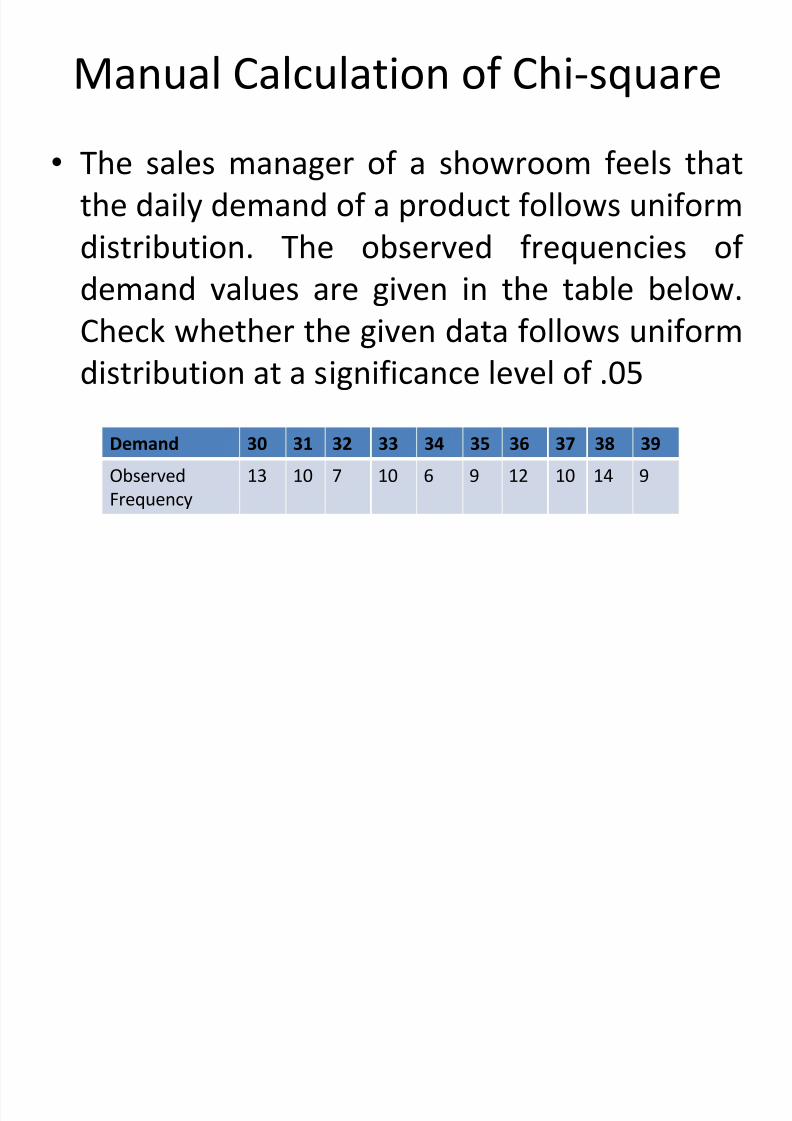
Manual Calculation of Chi-square
• The sales manager of a showroom feels that
the daily demand of a product follows uniform
distribution. The observed frequencies of
demand values are given in the table below.Check whether the given data follows uniform
distribution at a significance level of .05
Demand 30 31 32 33 34 35 36 37 38 39
Observed
Frequency
13 10 7 10 6 9 12 10 14 9
7/15/2019 Simple Tabulation 7and.ppt
http://slidepdf.com/reader/full/simple-tabulation-7andppt 14/52
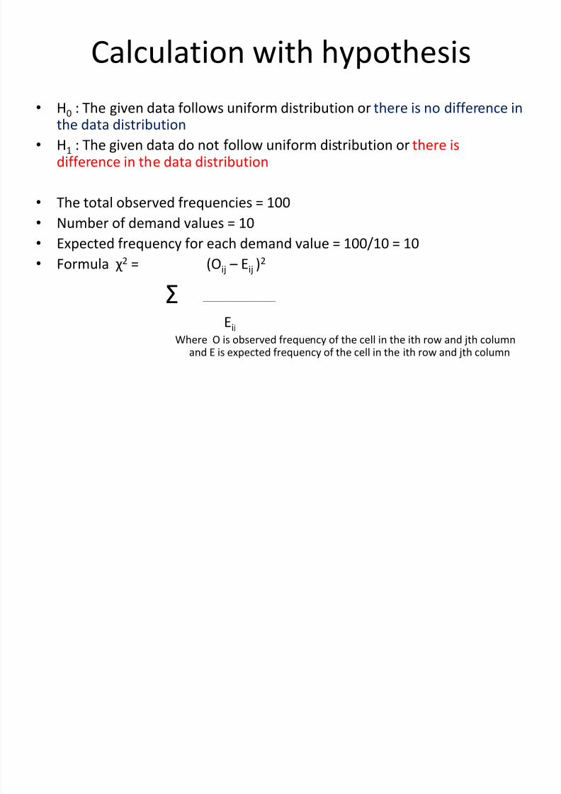
Calculation with hypothesis
• H0 : The given data follows uniform distribution or there is no difference inthe data distribution
• H1 : The given data do not follow uniform distribution or there isdifference in the data distribution
• The total observed frequencies = 100
• Number of demand values = 10
• Expected frequency for each demand value = 100/10 = 10
• Formula χ 2 = (Oij – Eij )2
Σ ____________________________
Ei j
Where O is observed frequency of the cell in the ith row and jth columnand E is expected frequency of the cell in the ith row and jth column
7/15/2019 Simple Tabulation 7and.ppt
http://slidepdf.com/reader/full/simple-tabulation-7andppt 15/52
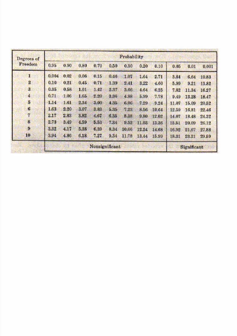
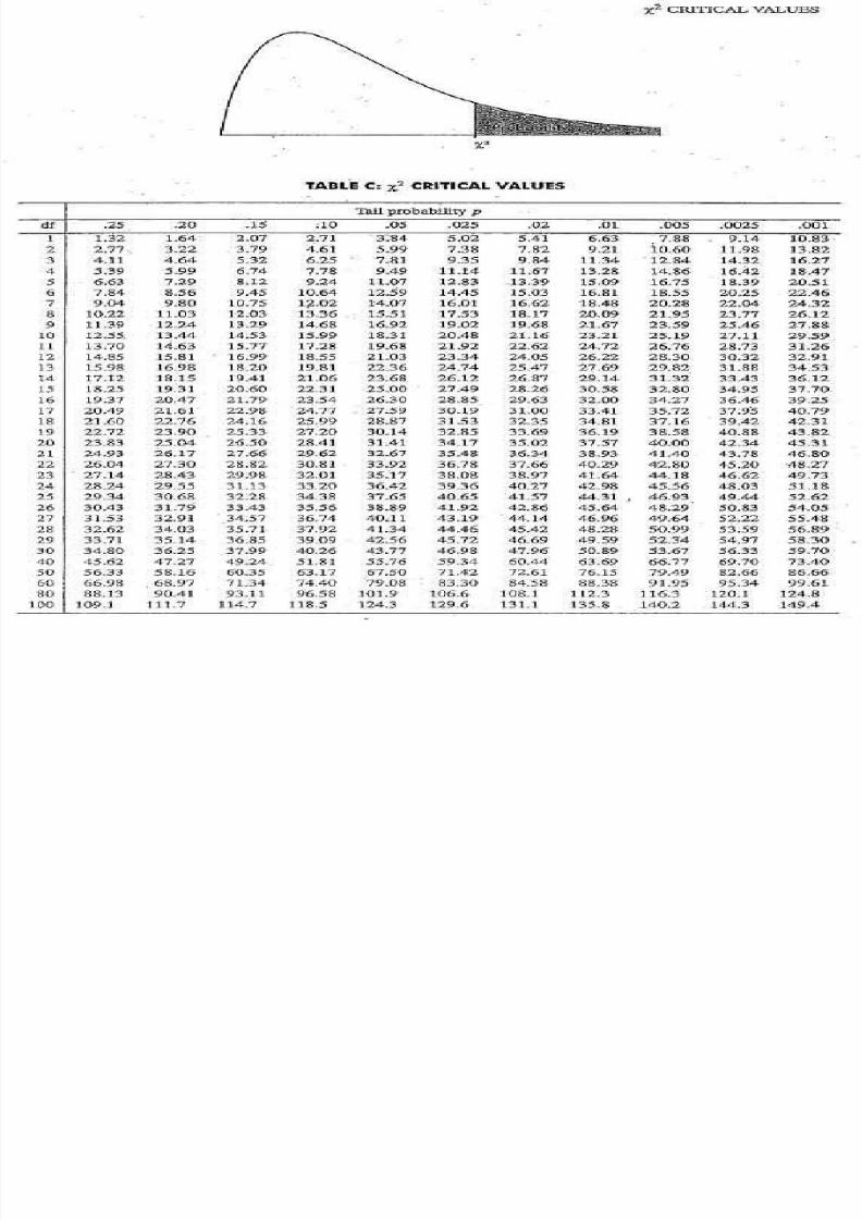
Intrepretation of Chi-square value
• if calculated value is less than table value
accept the H0 and reject the H1
• if calculated value is more than table value
accept the H1 and reject the H0

7/15/2019 Simple Tabulation 7and.ppt
http://slidepdf.com/reader/full/simple-tabulation-7andppt 16/52
Degree of Freedom Determination
• If there are 10 frequency classes and there is
one independent constraint, then there are
(10-1) = 9 Degree of Freedom.
7/15/2019 Simple Tabulation 7and.ppt
http://slidepdf.com/reader/full/simple-tabulation-7andppt 17/52
7/15/2019 Simple Tabulation 7and.ppt
http://slidepdf.com/reader/full/simple-tabulation-7andppt 18/52
7/15/2019 Simple Tabulation 7and.ppt
http://slidepdf.com/reader/full/simple-tabulation-7andppt 19/52
Hypothesis
• H0 : The given data follows uniform distribution
• H1 : The given data does not follow uniform
distribution
7/15/2019 Simple Tabulation 7and.ppt
http://slidepdf.com/reader/full/simple-tabulation-7andppt 20/52
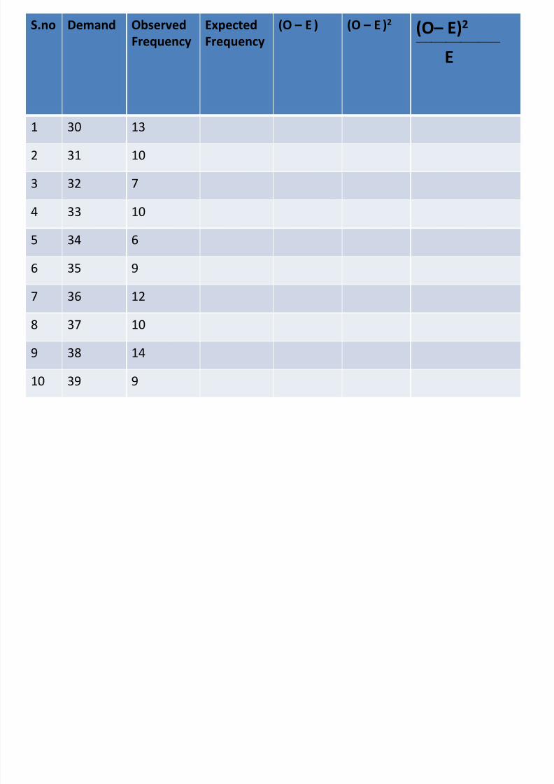
S.no Demand Observed
Frequency
Expected
Frequency
(O – E ) (O – E )2 (O – E)2
____________________________
E
1 30 13
2 31 10
3 32 7
4 33 10
5 34 6
6 35 9
7 36 12
8 37 10
9 38 14
10 39 9

7/15/2019 Simple Tabulation 7and.ppt
http://slidepdf.com/reader/full/simple-tabulation-7andppt 21/52
S.no Demand Observed
Frequency
Expected
Frequency
(O – E ) (O – E )2 (O – E)2
____________________________
E
1 30 13 10
2 31 10 10
3 32 7 10
4 33 10 10
5 34 6 10
6 35 9 10
7 36 12 10
8 37 10 10
9 38 14 10
10 39 9 10
7/15/2019 Simple Tabulation 7and.ppt
http://slidepdf.com/reader/full/simple-tabulation-7andppt 22/52
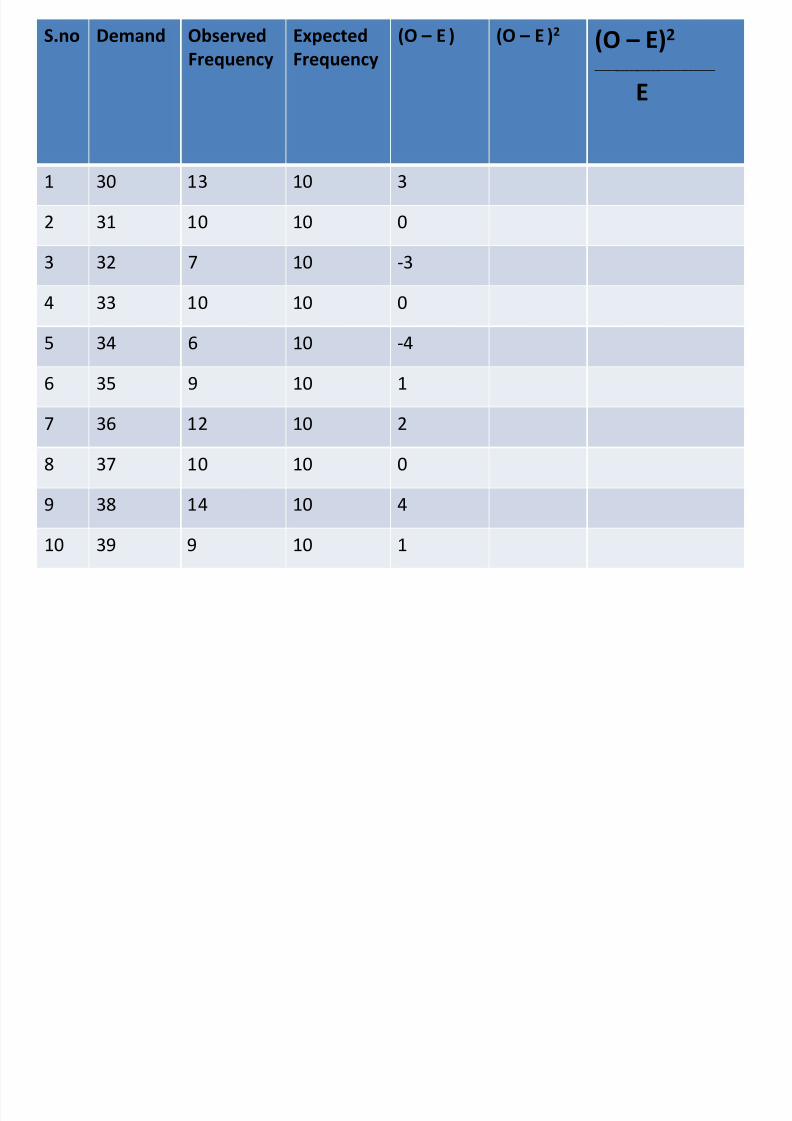
S.no Demand Observed
Frequency
Expected
Frequency
(O – E ) (O – E )2 (O – E)2
____________________________
E
1 30 13 10 3
2 31 10 10 0
3 32 7 10 -3
4 33 10 10 0
5 34 6 10 -4
6 35 9 10 1
7 36 12 10 2
8 37 10 10 0
9 38 14 10 4
10 39 9 10 1
7/15/2019 Simple Tabulation 7and.ppt
http://slidepdf.com/reader/full/simple-tabulation-7andppt 23/52
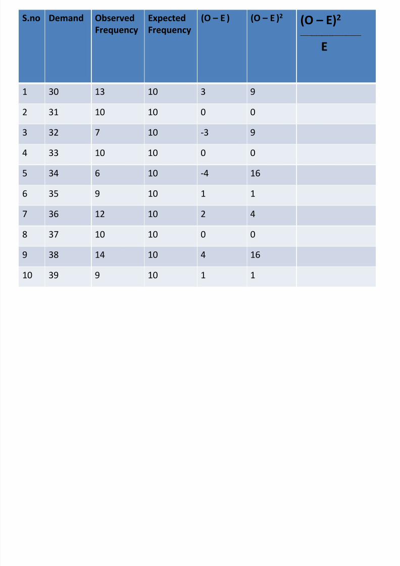
S.no Demand Observed
Frequency
Expected
Frequency
(O – E ) (O – E )2 (O – E)2
____________________________
E
1 30 13 10 3 9
2 31 10 10 0 0
3 32 7 10 -3 9
4 33 10 10 0 0
5 34 6 10 -4 16
6 35 9 10 1 1
7 36 12 10 2 4
8 37 10 10 0 0
9 38 14 10 4 16
10 39 9 10 1 1
7/15/2019 Simple Tabulation 7and.ppt
http://slidepdf.com/reader/full/simple-tabulation-7andppt 24/52
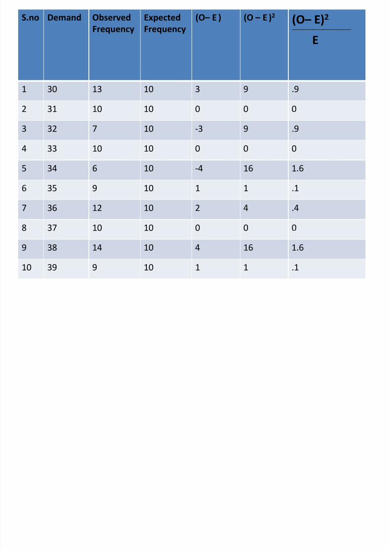
S.no Demand Observed
Frequency
Expected
Frequency
(O – E ) (O – E )2 (O – E)2
____________________________
E
1 30 13 10 3 9 .9
2 31 10 10 0 0 0
3 32 7 10 -3 9 .9
4 33 10 10 0 0 0
5 34 6 10 -4 16 1.6
6 35 9 10 1 1 .1
7 36 12 10 2 4 .4
8 37 10 10 0 0 0
9 38 14 10 4 16 1.6
10 39 9 10 1 1 .1
7/15/2019 Simple Tabulation 7and.ppt
http://slidepdf.com/reader/full/simple-tabulation-7andppt 25/52
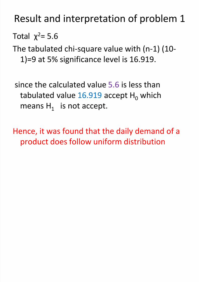
Result and interpretation of problem 1
Total χ 2= 5.6The tabulated chi-square value with (n-1) (10-
1)=9 at 5% significance level is 16.919.
since the calculated value 5.6 is less than
tabulated value 16.919 accept H0 which
means H1 is not accept.
Hence, it was found that the daily demand of a
product does follow uniform distribution
7/15/2019 Simple Tabulation 7and.ppt
http://slidepdf.com/reader/full/simple-tabulation-7andppt 26/52
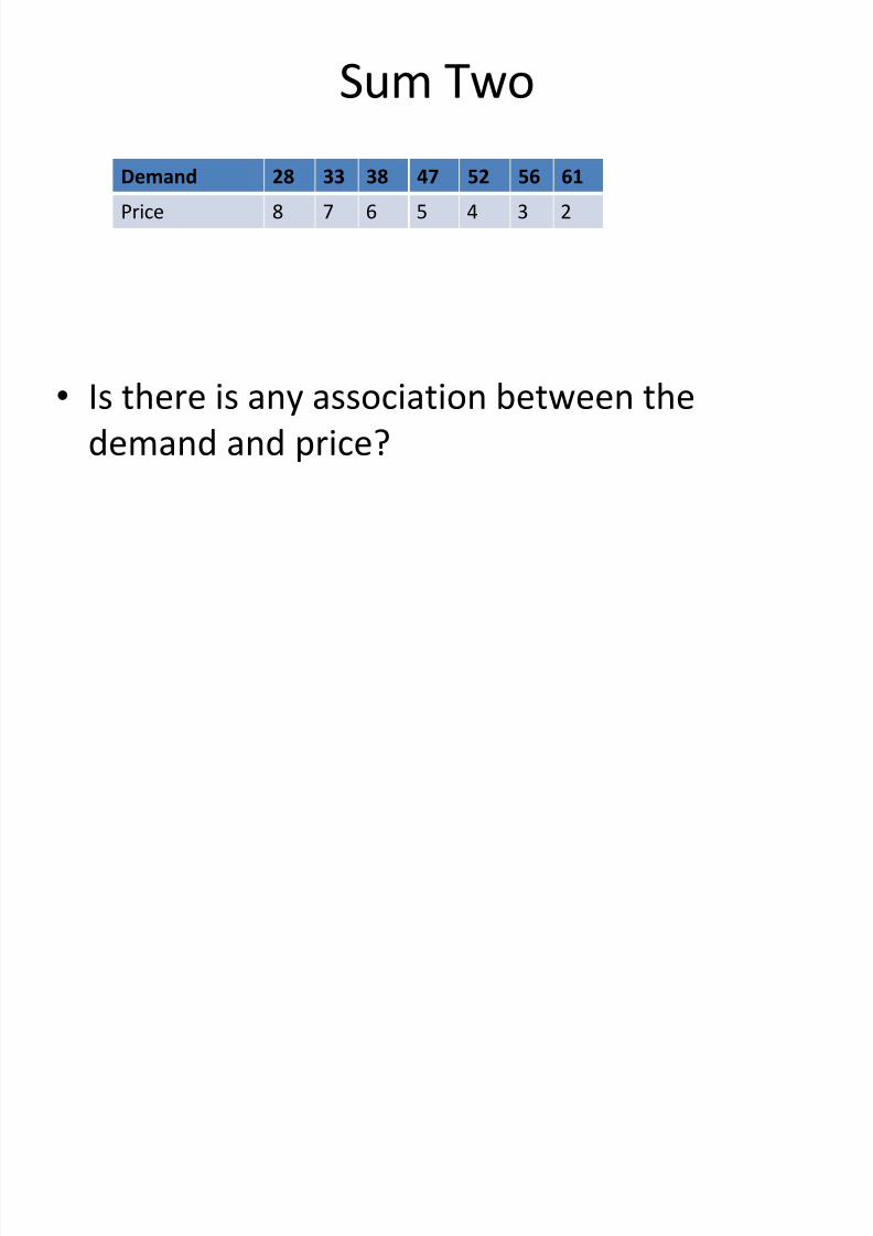
Sum Two
• Is there is any association between the
demand and price?
Demand 28 33 38 47 52 56 61
Price 8 7 6 5 4 3 2
7/15/2019 Simple Tabulation 7and.ppt
http://slidepdf.com/reader/full/simple-tabulation-7andppt 27/52
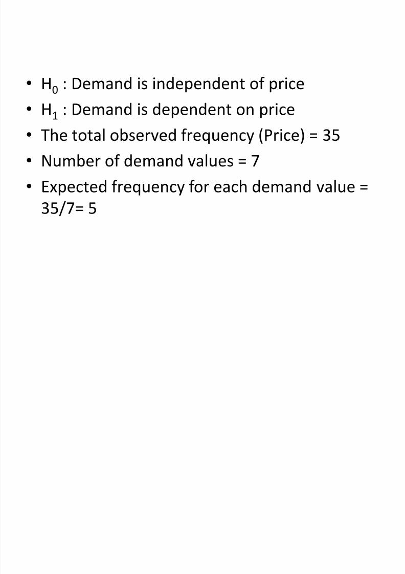
• H0 : Demand is independent of price
• H1 : Demand is dependent on price
•The total observed frequency (Price) = 35
• Number of demand values = 7
• Expected frequency for each demand value =
35/7= 5
7/15/2019 Simple Tabulation 7and.ppt
http://slidepdf.com/reader/full/simple-tabulation-7andppt 28/52
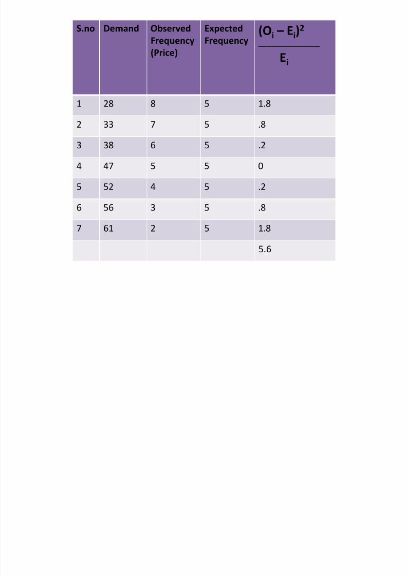
S.no Demand Observed
Frequency
(Price)
Expected
Frequency(Oi – Ei)
2
____________________________
Ei
1 28 8 5 1.8
2 33 7 5 .8
3 38 6 5 .2
4 47 5 5 0
5 52 4 5 .2
6 56 3 5 .8
7 61 2 5 1.8
5.6

7/15/2019 Simple Tabulation 7and.ppt
http://slidepdf.com/reader/full/simple-tabulation-7andppt 29/52
Interpretation of sum 2 result
• The table value with (7-1) = 6 DF at 5%
significance level is 12.591.
• Since the calculated value 5.6 is less than
tabulated value 12.591 accept H0, reject H1 ,
which means that demand is independent of
price.
7/15/2019 Simple Tabulation 7and.ppt
http://slidepdf.com/reader/full/simple-tabulation-7andppt 30/52
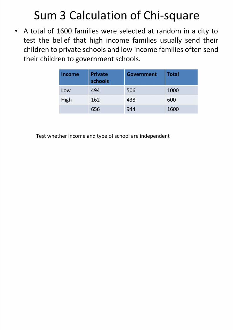
Sum 3 Calculation of Chi-square• A total of 1600 families were selected at random in a city to
test the belief that high income families usually send theirchildren to private schools and low income families often send
their children to government schools.
Income Private
schools
Government Total
Low 494 506 1000
High 162 438 600
656 944 1600
Test whether income and type of school are independent
7/15/2019 Simple Tabulation 7and.ppt
http://slidepdf.com/reader/full/simple-tabulation-7andppt 31/52
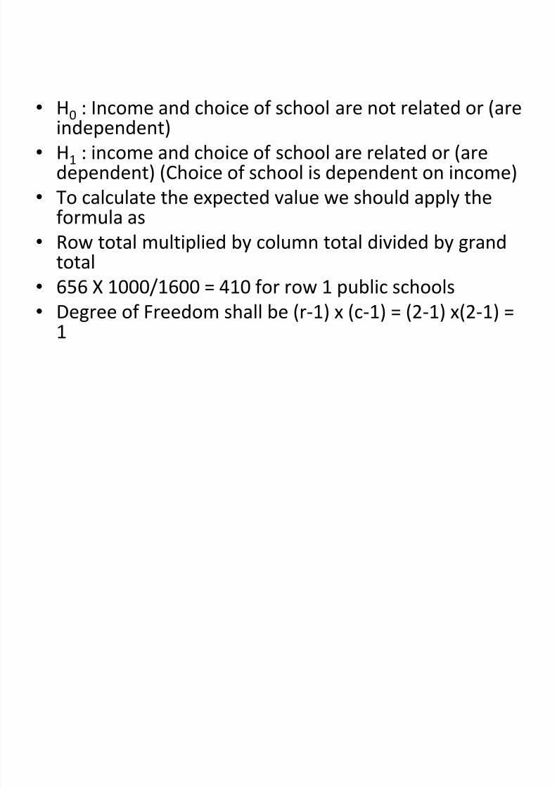
• H0 : Income and choice of school are not related or (areindependent)
• H1 : income and choice of school are related or (aredependent) (Choice of school is dependent on income)
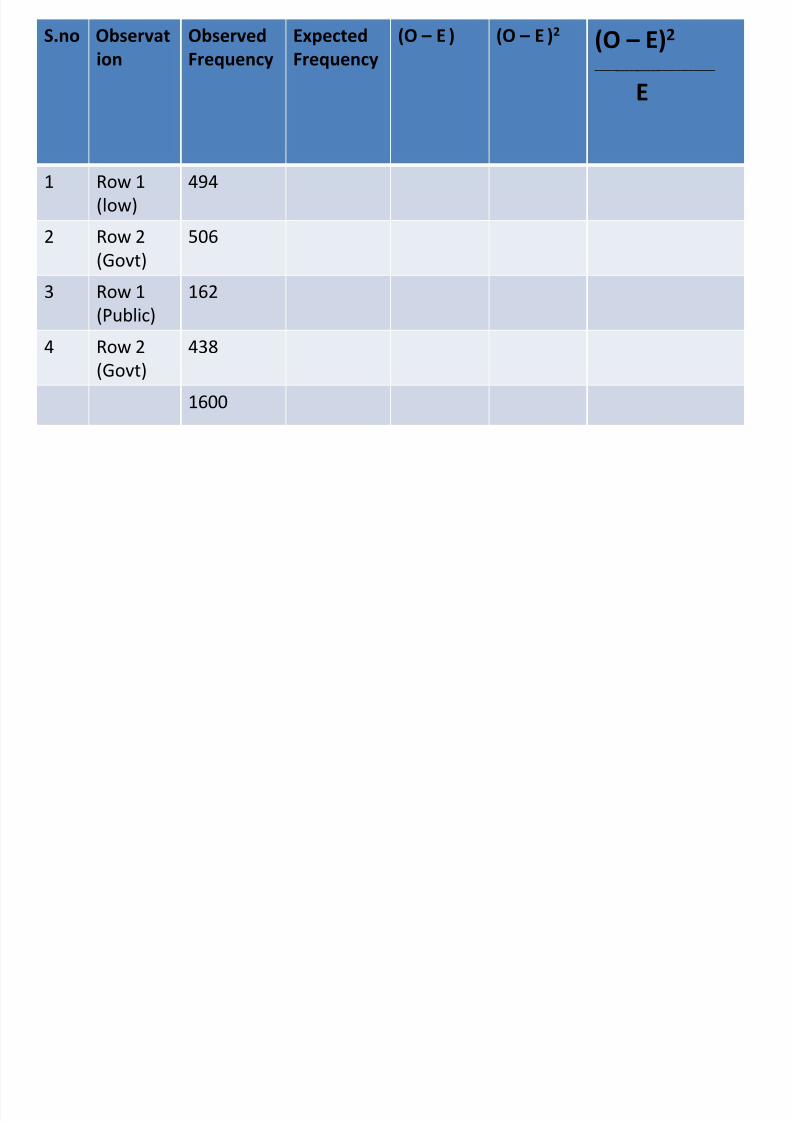
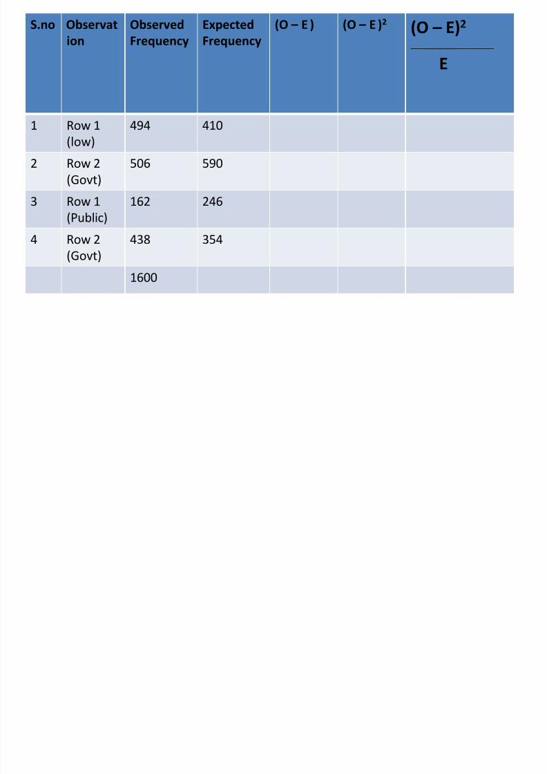
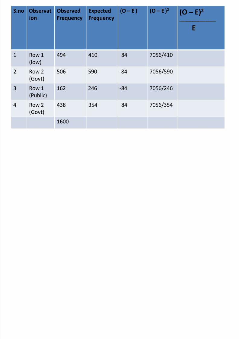
• To calculate the expected value we should apply theformula as
• Row total multiplied by column total divided by grandtotal
•656 X 1000/1600 = 410 for row 1 public schools
• Degree of Freedom shall be (r-1) x (c-1) = (2-1) x(2-1) =1
7/15/2019 Simple Tabulation 7and.ppt
http://slidepdf.com/reader/full/simple-tabulation-7andppt 32/52
S.no Observat
ion
Observed
Frequency
Expected
Frequency
(O – E ) (O – E )2 (O – E)2
____________________________
E
1 Row 1
(low)
494
2 Row 2
(Govt)
506
3 Row 1
(Public)
162
4 Row 2
(Govt)
438
1600
7/15/2019 Simple Tabulation 7and.ppt
http://slidepdf.com/reader/full/simple-tabulation-7andppt 33/52
S.no Observat
ion
Observed
Frequency
Expected
Frequency
(O – E ) (O – E )2 (O – E)2
____________________________
E
1 Row 1
(low)
494 410
2 Row 2
(Govt)
506 590
3 Row 1
(Public)
162 246
4 Row 2
(Govt)
438 354
1600

7/15/2019 Simple Tabulation 7and.ppt
http://slidepdf.com/reader/full/simple-tabulation-7andppt 34/52
S.no Observat
ion
Observed
Frequency
Expected
Frequency
(O – E ) (O – E )2 (O – E)2
____________________________
E
1 Row 1
(low)
494 410 84
2 Row 2
(Govt)
506 590 -84
3 Row 1
(Public)
162 246 -84
4 Row 2
(Govt)
438 354 84
1600
7/15/2019 Simple Tabulation 7and.ppt
http://slidepdf.com/reader/full/simple-tabulation-7andppt 35/52
S.no Observat
ion
Observed
Frequency
Expected
Frequency
(O – E ) (O – E )2 (O – E)2
____________________________
E
1 Row 1
(low)
494 410 84 7056/410
2 Row 2
(Govt)
506 590 -84 7056/590
3 Row 1
(Public)
162 246 -84 7056/246
4 Row 2
(Govt)
438 354 84 7056/354
1600
7/15/2019 Simple Tabulation 7and.ppt
http://slidepdf.com/reader/full/simple-tabulation-7andppt 36/52
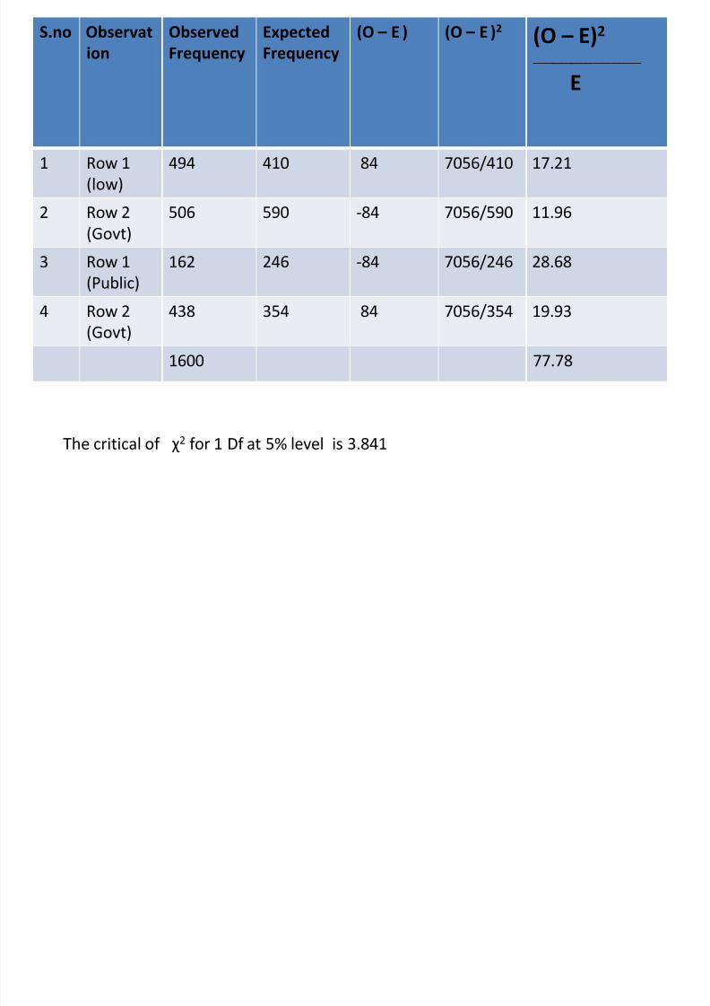
S.no Observat
ion
Observed
Frequency
Expected
Frequency
(O – E ) (O – E )2 (O – E)2
____________________________
E
1 Row 1
(low)
494 410 84 7056/410 17.21
2 Row 2
(Govt)
506 590 -84 7056/590 11.96
3 Row 1
(Public)
162 246 -84 7056/246 28.68
4 Row 2
(Govt)
438 354 84 7056/354 19.93
1600 77.78
The critical of χ 2 for 1 Df at 5% level is 3.841
7/15/2019 Simple Tabulation 7and.ppt
http://slidepdf.com/reader/full/simple-tabulation-7andppt 37/52
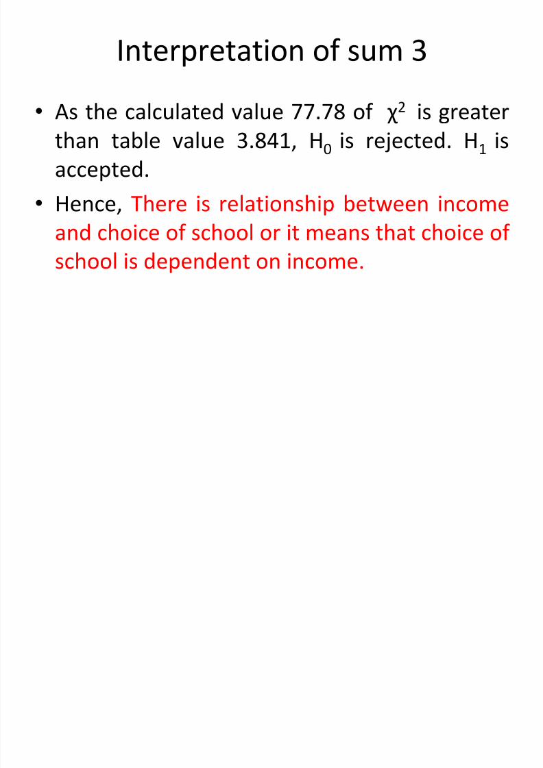
Interpretation of sum 3
• As the calculated value 77.78 of χ 2 is greater
than table value 3.841, H0 is rejected. H1 is
accepted.
• Hence, There is relationship between income
and choice of school or it means that choice of
school is dependent on income.
7/15/2019 Simple Tabulation 7and.ppt
http://slidepdf.com/reader/full/simple-tabulation-7andppt 38/52
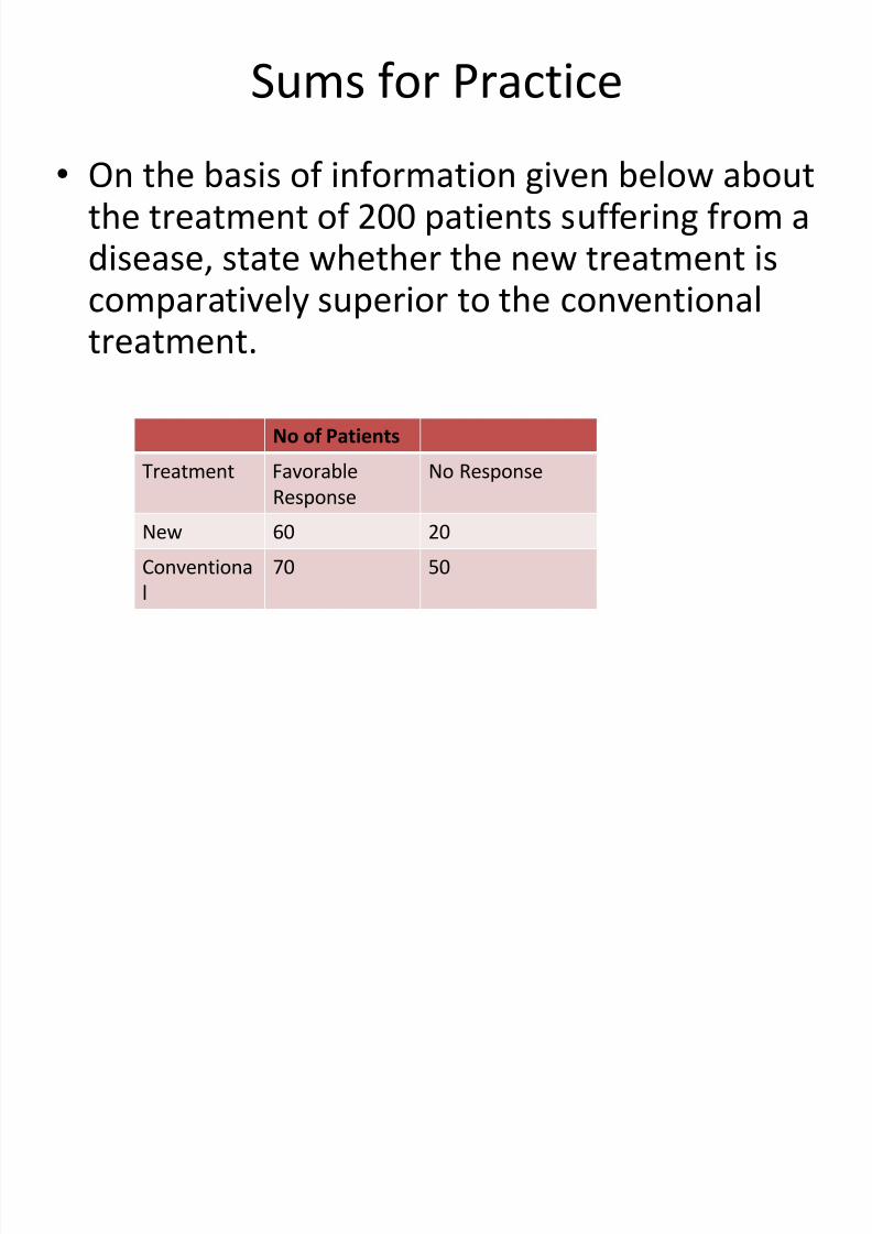
Sums for Practice
• On the basis of information given below aboutthe treatment of 200 patients suffering from adisease, state whether the new treatment is
comparatively superior to the conventionaltreatment.
No of Patients
Treatment Favorable
Response
No Response
New 60 20
Conventiona
l
70 50
7/15/2019 Simple Tabulation 7and.ppt
http://slidepdf.com/reader/full/simple-tabulation-7andppt 39/52
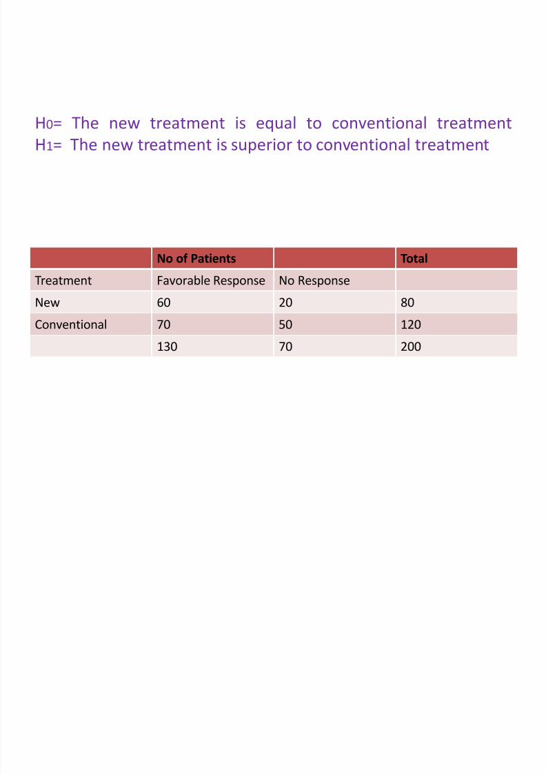
H0= The new treatment is equal to conventional treatment
H1= The new treatment is superior to conventional treatment
No of Patients Total
Treatment Favorable Response No Response
New 60 20 80
Conventional 70 50 120
130 70 200
2
7/15/2019 Simple Tabulation 7and.ppt
http://slidepdf.com/reader/full/simple-tabulation-7andppt 40/52
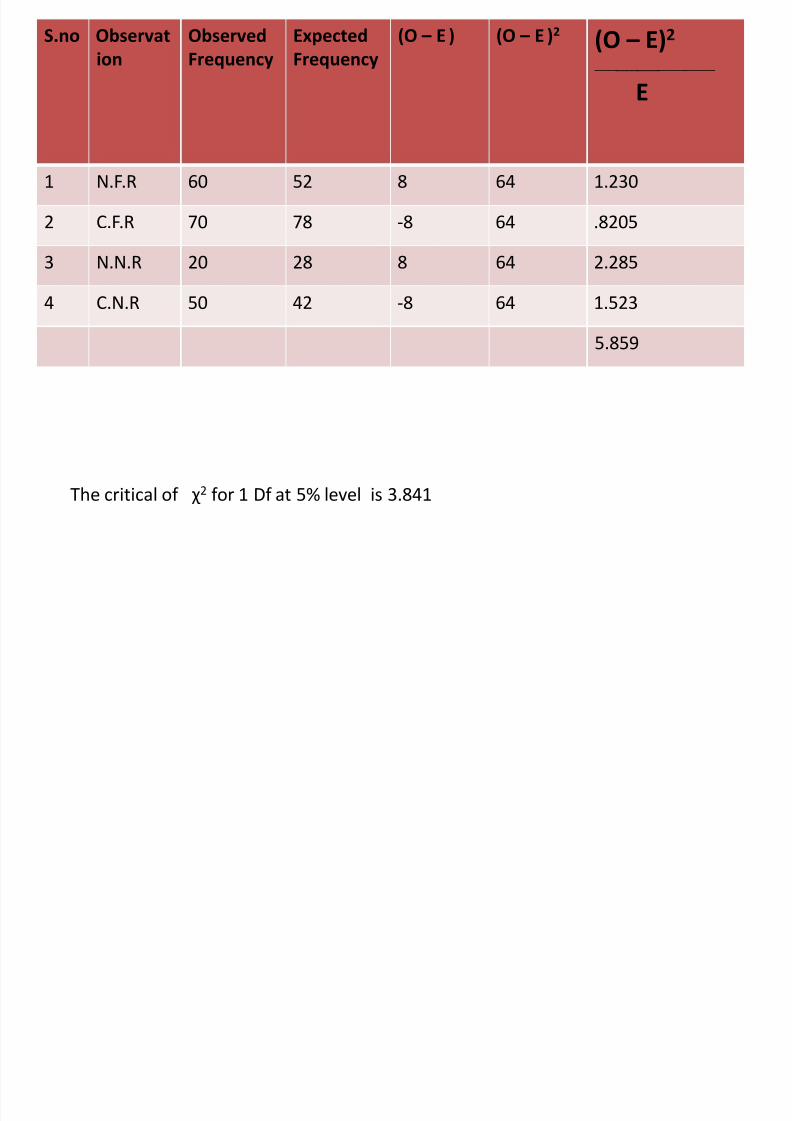
S.no Observat
ion
Observed
Frequency
Expected
Frequency
(O – E ) (O – E )2 (O – E)2
____________________________
E
1 N.F.R 60 52 8 64 1.230
2 C.F.R 70 78 -8 64 .8205
3 N.N.R 20 28 8 64 2.285
4 C.N.R 50 42 -8 64 1.523
5.859
The critical of χ 2 for 1 Df at 5% level is 3.841

7/15/2019 Simple Tabulation 7and.ppt
http://slidepdf.com/reader/full/simple-tabulation-7andppt 41/52
Interpretation of practice sum
• Since the calculated value 5.859 is more than
the table value of 3.84146, it was found that
H1 is accepted therefore, that the new
treatment is comparatively superior to theconventional treatment.
7/15/2019 Simple Tabulation 7and.ppt
http://slidepdf.com/reader/full/simple-tabulation-7andppt 42/52
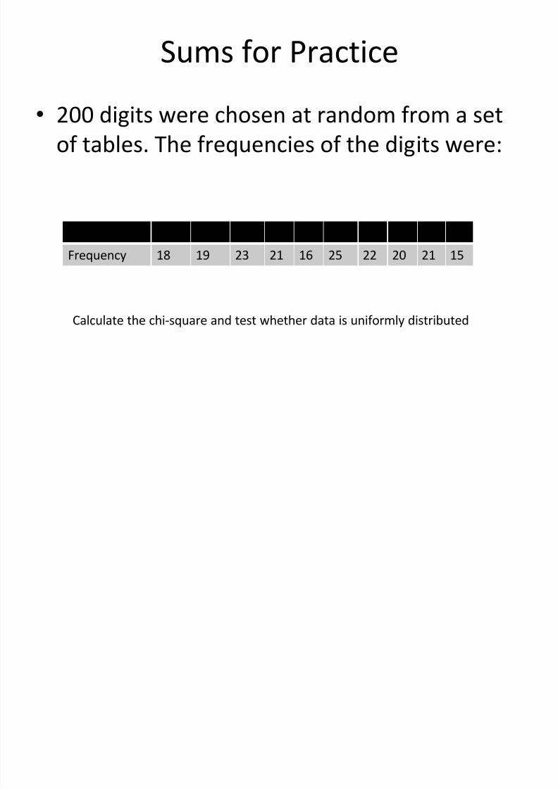
Sums for Practice
• 200 digits were chosen at random from a set
of tables. The frequencies of the digits were:
Digit 0 1 2 3 4 5 6 7 8 9
Frequency 18 19 23 21 16 25 22 20 21 15
Calculate the chi-square and test whether data is uniformly distributed
7/15/2019 Simple Tabulation 7and.ppt
http://slidepdf.com/reader/full/simple-tabulation-7andppt 43/52
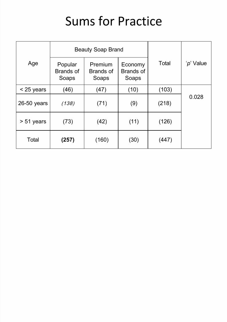
Sums for Practice
Age
Beauty Soap Brand
Total ‘ p’ Value Popular
Brands of
Soaps
Premium
Brands of
Soaps
Economy
Brands of
Soaps
< 25 years (46) (47) (10) (103)
0.028 26-50 years (138) (71) (9) (218)
> 51 years (73) (42) (11) (126)
Total (257) (160) (30) (447)
7/15/2019 Simple Tabulation 7and.ppt
http://slidepdf.com/reader/full/simple-tabulation-7andppt 44/52
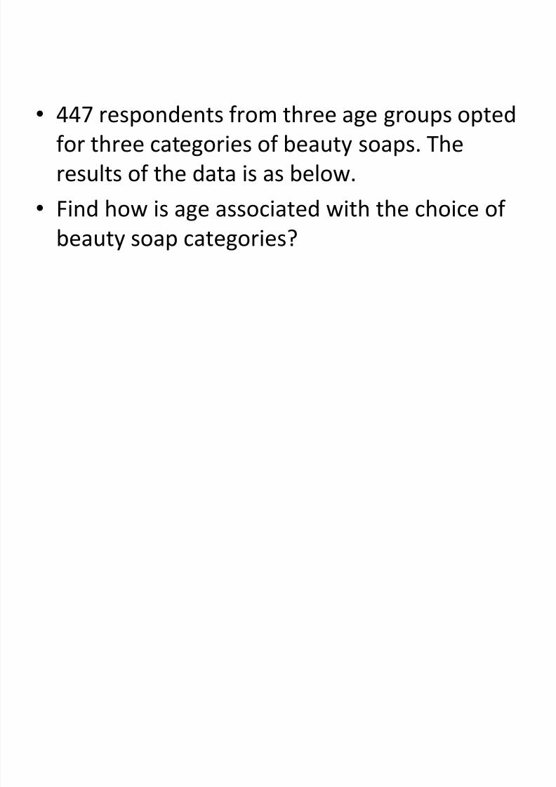
• 447 respondents from three age groups opted
for three categories of beauty soaps. The
results of the data is as below.
• Find how is age associated with the choice of
beauty soap categories?
7/15/2019 Simple Tabulation 7and.ppt
http://slidepdf.com/reader/full/simple-tabulation-7andppt 45/52
Hypothesis
• H0= Age has no influence on the choice of
different categories of beauty soap brands
• H1= There is influence of age on the choice on
different categories of beauty soap brands
7/15/2019 Simple Tabulation 7and.ppt
http://slidepdf.com/reader/full/simple-tabulation-7andppt 46/52
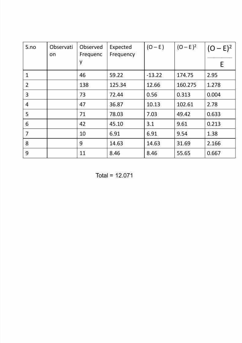
S.no Observati
on
Observed
Frequenc
y
Expected
Frequency
(O – E ) (O – E )2 (O – E)2
___________________
E
1 46 59.22 -13.22 174.75 2.95
2 138 125.34 12.66 160.275 1.2783 73 72.44 0.56 0.313 0.004
4 47 36.87 10.13 102.61 2.78
5 71 78.03 7.03 49.42 0.633
6 42 45.10 3.1 9.61 0.213
7 10 6.91 6.91 9.54 1.38
8 9 14.63 14.63 31.69 2.166
9 11 8.46 8.46 55.65 0.667
Total = 12.071
A l i
7/15/2019 Simple Tabulation 7and.ppt
http://slidepdf.com/reader/full/simple-tabulation-7andppt 47/52
• The calculated value 12.071 is more than 9.49
Df at 5% level is 9.49, therefore H1 is
accepted. Hence, it is concluded that age
influences the choice of different categories of beauty soap brands.
Analysis
7/15/2019 Simple Tabulation 7and.ppt
http://slidepdf.com/reader/full/simple-tabulation-7andppt 48/52
To Obtain a Chi-Square Test
• From the menus choose:
• AnalyzeNonparametric Tests
Chi-Square...• Select one or more test variables. Each
variable produces a separate test.
• Optionally, you can click Options fordescriptive statistics, quartiles, and control of the treatment of missing data.
7/15/2019 Simple Tabulation 7and.ppt
http://slidepdf.com/reader/full/simple-tabulation-7andppt 49/52
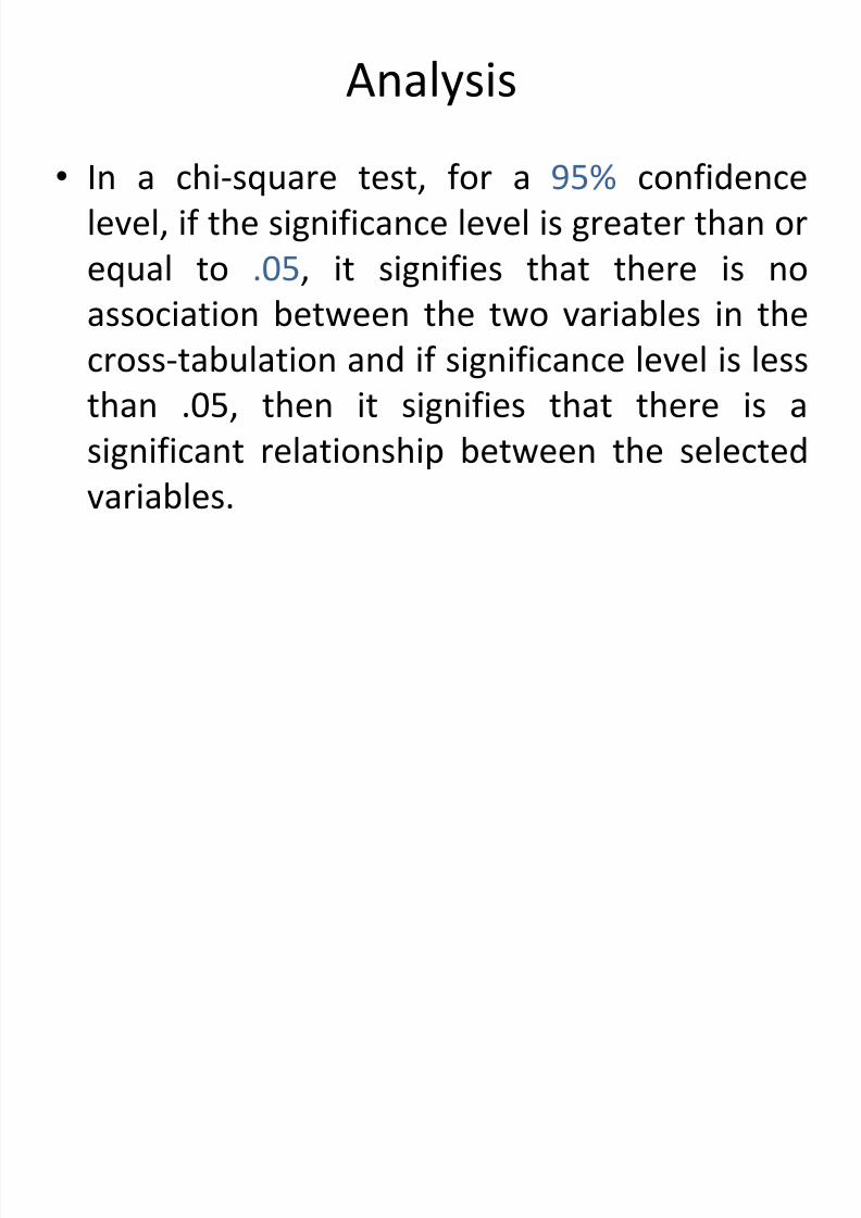
Analysis
• In a chi-square test, for a 95% confidence
level, if the significance level is greater than or
equal to .05, it signifies that there is no
association between the two variables in thecross-tabulation and if significance level is less
than .05, then it signifies that there is a
significant relationship between the selectedvariables.
7/15/2019 Simple Tabulation 7and.ppt
http://slidepdf.com/reader/full/simple-tabulation-7andppt 50/52
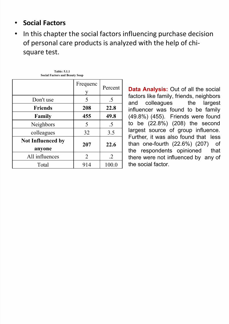
• Social Factors
• In this chapter the social factors influencing purchase decision
of personal care products is analyzed with the help of chi-square test.
Frequenc
y Percent
Don't use 5 .5
Friends 208 22.8
Family 455 49.8
Neighbors 5 .5
colleagues 32 3.5
Not Influenced by
anyone 207 22.6
All influences 2 .2
Total 914 100.0
Table: 5.1.1
Social Factors and Beauty Soap
Data Analysis: Out of all the social
factors like family, friends, neighbors
and colleagues the largest
influencer was found to be family
(49.8%) (455). Friends were found
to be (22.8%) (208) the secondlargest source of group influence.
Further, it was also found that less
than one-fourth (22.6%) (207) of
the respondents opinioned that
there were not influenced by any of
the social factor.
Chi l i i SPSS

7/15/2019 Simple Tabulation 7and.ppt
http://slidepdf.com/reader/full/simple-tabulation-7andppt 51/52
Chi-square analysis using SPSS
Value df
Asymp.
Sig. (2-
sided)
Pearson Chi-
Square 466.042(a) 180 .000
Likelihood Ratio 387.650 180 .000
Linear-by-Linear
Association 20.258 1 .000
N of Valid Cases 913
Value
Asym
p. Std.
Error(
a)
Appro
x. T(b)
Approx
. Sig.
Nominal by
Nominal
Contingency
Coefficient
.581 .000
N of Valid Cases 913
Table: 5.1.2
Social Factors and Beauty Soap
.
Table: 5.1.3
Social Factors and Beauty Soap
(In the chi-square test, for a 95 percent confidence
level, if the significance level is greater than or
equal to .05, it signifies that there is no associationbetween the two variables and the if significance
level is less than .05, then it signifies that there is a
significant relationship between the two variables.)
At 95 percent confidence level, with 180 degree of
freedom the above analysis demonstrates
significant association between social factors and
beauty soap. The calculated value .000 is less
than the standard value .05. From the obtained
contingency coefficient value of .581, it may be
inferred that the association between the
dependent and independent variable is significant,
as the value .581 is closer to 1 than to 0.
7/15/2019 Simple Tabulation 7and.ppt
http://slidepdf.com/reader/full/simple-tabulation-7andppt 52/52
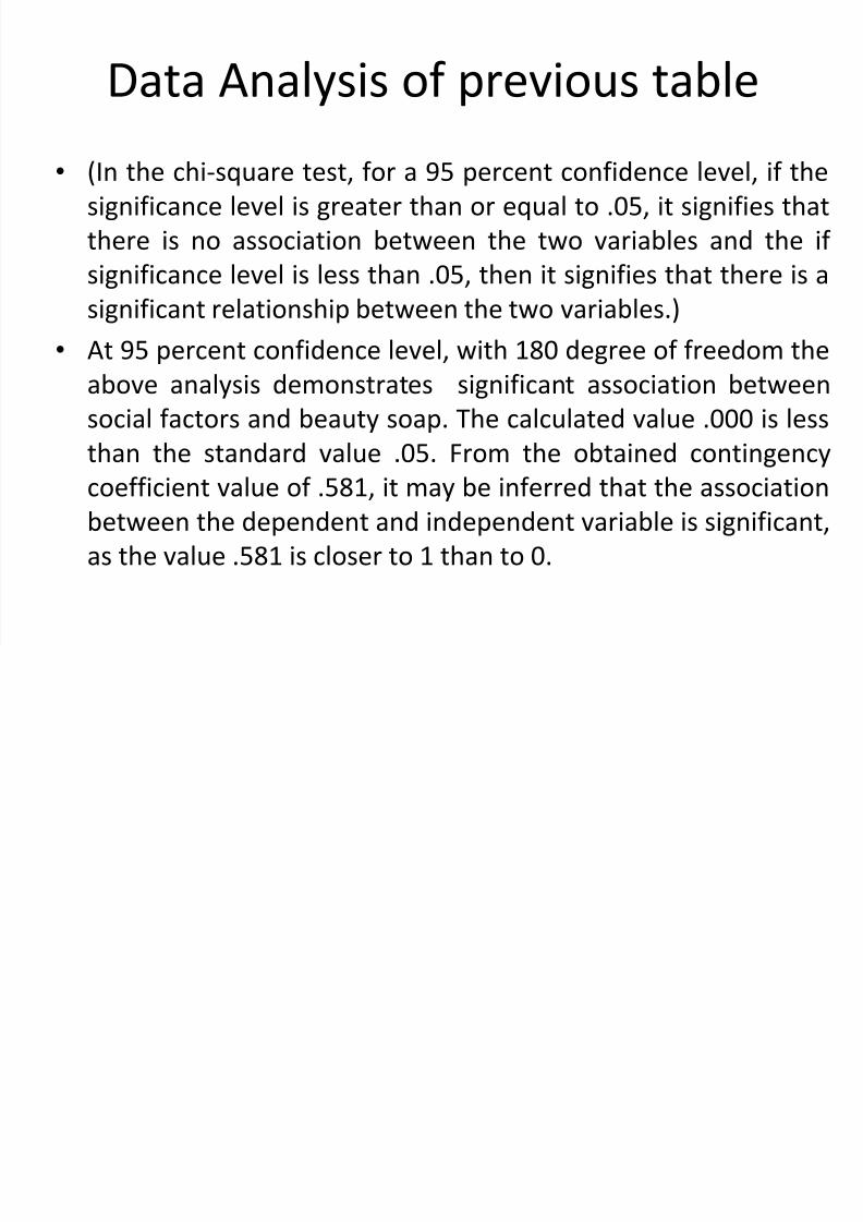
Data Analysis of previous table
• (In the chi-square test, for a 95 percent confidence level, if the
significance level is greater than or equal to .05, it signifies that
there is no association between the two variables and the if
significance level is less than .05, then it signifies that there is a
significant relationship between the two variables.)• At 95 percent confidence level, with 180 degree of freedom the
above analysis demonstrates significant association between
social factors and beauty soap. The calculated value .000 is less
than the standard value .05. From the obtained contingencycoefficient value of .581, it may be inferred that the association
between the dependent and independent variable is significant,
as the value .581 is closer to 1 than to 0.