Simple TCP Protocol Simulator - ece.rutgers.edumarsic/books/CN/projects/tcp/tcp-sim... · 1 The Design of a Simple TCP Simulator 3 3 bufferCapacity_ (currently set at 6 packet slots),

Last updated: December 8, 2014

Simple TCP Protocol

Simulator

With Programming Assignments for a Computer Networks Course

Ivan Marsic

Copyright © 2005 – 2014 by Ivan Marsic. All rights reserved.

Rutgers University, New Brunswick, New Jersey

Permission to reproduce or copy all or parts of this material for non-profit use is granted on the condition that the author and source are credited.

Author’s address:

Ivan Marsic Rutgers University Department of Electrical and Computer Engineering 94 Brett Road Piscataway, New Jersey 08854 [email protected]

Book website: http://www.ece.rutgers.edu/~marsic/books/CN/

iii

Table of Contents

TABLE OF CONTENTS...........................................................................................................................III

1 THE DESIGN OF A SIMPLE TCP SIMULATOR.......................................................................... 1

1.1 INTRODUCTION .............................................................................................................................. 2 1.1.1 How to Run the Simulator......................................................................................................... 2 1.1.2 User Interface and Reporting ................................................................................................... 3

1.2 TIME SIMULATION ......................................................................................................................... 3 1.2.1 Simulation Engine Logic........................................................................................................... 4 1.2.2 Simulated Timers ...................................................................................................................... 8

1.3 NETWORK MODELING ................................................................................................................. 10 1.3.1 Network Elements ................................................................................................................... 11 1.3.2 Router Design......................................................................................................................... 13 1.3.3 Configuring and Running the Network................................................................................... 16

1.4 TCP PROTOCOL COMPONENTS .................................................................................................... 18 1.4.1 TCP Sender............................................................................................................................. 20 1.4.2 Sender States .......................................................................................................................... 21 1.4.3 Timeout Interval Estimation ................................................................................................... 24 1.4.4 TCP Receiver.......................................................................................................................... 26

1.5 SUPPORTED VERSIONS OF TCP.................................................................................................... 27 1.5.1 TCP Tahoe.............................................................................................................................. 28 1.5.2 TCP Reno................................................................................................................................ 28 1.5.3 TCP NewReno ........................................................................................................................ 29

2 PROGRAMMING ASSIGNMENTS............................................................................................... 31

2.1 ASSIGNMENT 1: UNLIMITED QUEUE AND BANDWIDTH BOTTLENECK.......................................... 33 2.1.1 Software Modification Description......................................................................................... 33 2.1.2 Experiment Description.......................................................................................................... 34

2.2 ASSIGNMENT 2: PACKET REORDERING DURING TRANSIT............................................................ 35 2.2.1 Software Modification Description......................................................................................... 36 2.2.2 Experiment Description.......................................................................................................... 37

2.3 ASSIGNMENT 3: VARIABLE OCCUPANCY OF THE ROUTER BUFFER.............................................. 38 2.3.1 Software Modification Description......................................................................................... 38 2.3.2 Experiment Description.......................................................................................................... 39

2.4 ASSIGNMENT 4: CONCURRENT TCP AND UDP FLOWS ................................................................ 40 2.4.1 Software Modification Description......................................................................................... 41 2.4.2 Experiment Description.......................................................................................................... 42

2.5 ASSIGNMENT 5: COMPETING TCP FLOWS AND FAIRNESS............................................................ 43 2.5.1 Software Modification Description......................................................................................... 43

Ivan Marsic Rutgers University

iv

2.5.2 Experiment Description.......................................................................................................... 44 2.6 ASSIGNMENT 6: ACTIVE QUEUE MANAGEMENT POLICY ............................................................. 45

2.6.1 Software Modification Description......................................................................................... 45 2.6.2 Experiment Description.......................................................................................................... 46

3 REFERENCES .................................................................................................................................. 48

1

Contents 1.1 Introduction

1.1.1 How to Run the Simulator 1.1.2 User Interface and Reporting

1.2 Time Simulation

1.2.1 Simulation Engine Logic 1.2.2 Simulated Timers

1.3 Network Modeling

1.3.2 Network Elements 1.3.2 Router Design 1.3.3 Configuring and Running the Network

1.5 TCP Protocol Components 1.4.1 TCP Sender 1.4.2 Sender States 1.4.3 Timeout Interval Estimation 1.4.4 TCP Receiver

1.5 Supported Versions of TCP 1.5.1 TCP Tahoe 1.5.2 TCP Reno 1.5.3 TCP NewReno

1 The Design of a Simple TCP Simulator

Transmission Control Protocol (TCP) is a core Internet protocol. Along with the Internet Protocol (IP), TCP/IP are the most frequently used protocols in the Internet. This document describes a simple implementation of TCP congestion control in the Java programming language.

One may wonder why develop another network simulator when there are so many great network simulator already out there, such as ns-2 (http://www.isi.edu/nsnam/ns/) and ns-3 (http://www.nsnam.org/). The reason is that I wanted to have a simple TCP simulator for instructional purposes—something comprehensible by a student taking a semester-long undergraduate course in computer networks. I believe that this simulator meets such a requirement. Despite its simplicity and many limitations, it supports many interesting scenarios to gain deep understanding of the TCP protocol in operation. This simulator is not intended for research proposes, as are ns-2 and ns-3, which provide power and flexibility. Unfortunately, they are also time-consuming to learn and use. And, such power and flexibility are not needed for an undergraduate course.

This document assumes that the reader is knowledgeable about the TCP protocol. Details about TCP can be found in my networking book available on the same website where this software is found.

The length of this document should not intimidate you to think that this simulator is not that simple. The only reason that this document is relatively long for such a simple program is that I wanted to describe in detail how the simulator works, what are its limitations, and what design choices were made and why. Describing all the simplifications and design compromises takes space, but I believe that the program itself is simple.


2

1.1 Introduction

This software implements a simple TCP simulator in the Java programming language. It does not implement all aspects of the TCP protocol, but rather focuses on the key aspects of TCP congestion control. A concise description of TCP implementation is available in [McKusick, et al., 1996, Chapter 13] and full details are available in [Wright & Stevens, 1995]. Our simulated network consists of network elements such as endpoint hosts and routers. The default configuration has two endpoints (sender-host and receiver-host) and single router, connected in a chain (also see Figure 4):

SENDER link1 NETWORK/ROUTER link2 RECEIVER

Our default implementation uses unidirectional transmission: the sender endpoint sends only data segments (not acknowledgments) and the receiver endpoint only replies with acknowledgments. Configurations that are more complex are possible, as described in Section 1.3.3.

This document explains the design of the simulator. The reader should check the Java source code for implementation details.

The student will need to know only the simulator main class (Section 1.2) and the network/router class (Section 1.3) for the programming assignments described in Section 2. The description of the TCP components is provided mainly for reference and I believe they can be used without modification.

Due to the time constraints, I was unable to achieve the best possible design or implement all TCP protocol details. Unfortunately, there are some kludges and unfinished features. The ambitious reader may wish to search for to-do notes (see //TODO comments) in the code and improve upon these deficiencies. I focused on the correct implementation of the TCP protocol congestion control and the compromises are mostly made for other network components.

1.1.1 How to Run the Simulator

The main class is Simulator.java. The program accepts two arguments on the command line:

The first argument is a string specifying the TCP sender type (must be one of these: “Tahoe” or “Reno” or “NewReno”). Enter the exact string, starting with the capital letter and the remaining letters in lower case.

The second argument specifies the number of iterations to run the simulation.

The application is bulk-data transfer of 1,000,000 bytes (see the field TOTAL_DATA_LENGTH in the class Simulator.java). If the sender completes transmitting all the data within the specified number of iterations, the simulator will start printing the message “Input bytestream empty -- nothing left to send” from the method send() in the class tcp.Sender.java.

Some other parameters, initialized in the method Simulator.main(), that you may consider exposing and making configurable from the user interface include:


3

3

bufferCapacity_ (currently set at 6 packet slots), which is the size of the router’s memory available for queuing packets from the simulated TCP session. In addition, one of our packets can be in transmission (see Figure 7) and some small space is allocated for acknowledgments. Note that currently we do not take into account packet header size—only packet payload is counted towards router buffer occupancy

rcvWindow_ (currently set at 65,536 bytes or 64 KBytes), which is the memory space allocated the receiver endpoint for buffering packets that arrived out-of-order (we assume that in-order packets will be immediately delivered to the application)

These parameters are described in the following sections. The choice of the default values is based on Example 2.1 in the book (Section 2.2).

In addition, the method Simulator.main() we create a dummy input buffer that will be sent to the receiver, the variable called inputBuffer. In reality, the data should be read from a file or another input stream.

Finally, all parameters for configuring the network model (Section 1.3.3), such as link transmission and propagation delays could be exposed in the user interface.

1.1.2 User Interface and Reporting

At this point, the simulator does not have any graphical user interface. As described in Section 1.1.1, it is run from a command line or from a development environment, such as Eclipse. If I had time, I would build a wizard for building the network model; see http://en.wikipedia.org/wiki/Wizard_(software).

Reporting for debugging and data collection is controlled by the attribute currentReportingLevel of Simulator.java. Setting this parameter to zero turns off all debugging-related reporting and only the values of the TCP congestion control parameters are outputted for every iteration. See the source code for other options.

1.2 Time Simulation

According to the Wikipedia page (http://en.wikipedia.org/wiki/Discrete_event_simulation), this simulator would rather qualify as continuous simulation instead of discrete event simulation (DES). This simulator is time-driven instead of event-driven. In this simulator, time is broken up into small slices (clock ticks) and the system state is updated according to the set of activities happening in each time slice. Unlike this, in discrete-event simulation time “jumps” to the start time of the next event whenever that may be, instead of regular clock ticks. In addition, events in DES are instantaneous—once the simulator starts processing an event, the time does not progress forward—the time will simply jump to the start of the next event.

The key function of a simulator is to simulate the passage of time. In a time-driven simulator, we need to decide about the duration of simulated clock ticks. In the default implementation, I chose


4

the tick to correspond to one round-trip time (RTT, from a TCP sender to a TCP receiver and back), which also represents one iteration of the simulation. This is the simplest choice, but the software components are implemented in a time-agnostic manner, so they could run with no program code modification (or perhaps only a little) with any tick duration in either continuous simulation or discrete event simulation. Section 1.3.3 discusses how to modify the tick duration. Even if we were to implement this simulator as discrete event simulation, then each component would need to know how long its activity takes, so that it can arrange the future events.

There are important advantages of event-driven simulation and most current network simulators are implemented as discrete event simulation (DES) [Banks, et al., 2005]. The reason that our simulation time marches in fixed intervals (clock ticks) is that I thought it would be simpler to implement (and probably easier to understand) a time-driven simulator. As a result, simulating different network models and communication protocols is simply not feasible with this simulator, but that is the price of simplicity and targeted purpose of learning TCP congestion control.

1.2.1 Simulation Engine Logic

The architecture of the simulator is shown Figure 1. The key components are four Java objects (Simulator, Sender, Router, and Receiver), of which Simulator.java is the main class that orchestrates the work of others as the time marches forward. The action sequence in Figure 2

TCP Sender

TCP Receiver

Network(single router)

Application Application

one simulation iteration = N clock ticks = one round-trip time

START

Simulator infrastructure (time progression)

Network layer protocol (IP)

Figure 1: The architecture of our TCP protocol simulator. The bottom part shows that onesimulation round represents one clock tick, which is one RTT long.


5

5

illustrates the operational logic of the simulator. It repeatedly cycles around visiting in turn Sender, Router, and Receiver. Simulator just calls the method process() on each network element and the elements themselves exchange data as appropriate. The software interface of our network elements is described in Section 1.3.1.

The simulator operational logic is represented in the class Simulator.java and the pseudo code is as follows:

Listing 1: Pseudo code of the simulation engine’s operational logic.

Start: // in the method Simulator.main() -

Initialize the system parameters (TCP version, number of iterations, communication link parameters, router buffer sizes, and TCP receive window sizes)

Initialize system state variable s (The Simulator class constructor creates the network model—endpoints, routers, and links—and

configures them in the initial state)

Initialize the clock (the simulation main loop starts at time zero)

The main loop: // in the method Simulator.run() -

Pass the reference to the application data bytestream to the sending endpoint.

For (given number of iterations) do the following:

1.1.2.2.

3.3. 4.4. 1.1.

Sender Router Receiver

Simulator

Anything to send?


Simulator

Relay packets


Simulator

Handle segments,

return ACKs

Returning ACKs or

duplic-ACKs


Simulator

Handle ACKs& send

segments

A B

C D

if EW 1send EW segments

relay # packets memory size; drop the excess.

Check if pktsin-order, store

if gaps

if EW 1send EW segments

EW = EW = EffectiveWindowEffectiveWindow

Figure 2: Action sequence illustrating how the Simulator object orchestrates the work of other software objects (shown are only first four steps of a simulation).


6

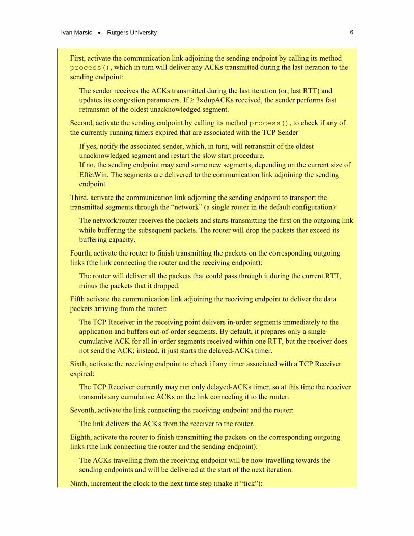
First, activate the communication link adjoining the sending endpoint by calling its method process(), which in turn will deliver any ACKs transmitted during the last iteration to the sending endpoint:

The sender receives the ACKs transmitted during the last iteration (or, last RTT) and updates its congestion parameters. If 3dupACKs received, the sender performs fast retransmit of the oldest unacknowledged segment.

Second, activate the sending endpoint by calling its method process(), to check if any of the currently running timers expired that are associated with the TCP Sender

If yes, notify the associated sender, which, in turn, will retransmit of the oldest unacknowledged segment and restart the slow start procedure. If no, the sending endpoint may send some new segments, depending on the current size of EffctWin. The segments are delivered to the communication link adjoining the sending endpoint.

Third, activate the communication link adjoining the sending endpoint to transport the transmitted segments through the “network” (a single router in the default configuration):

The network/router receives the packets and starts transmitting the first on the outgoing link while buffering the subsequent packets. The router will drop the packets that exceed its buffering capacity.

Fourth, activate the router to finish transmitting the packets on the corresponding outgoing links (the link connecting the router and the receiving endpoint):

The router will deliver all the packets that could pass through it during the current RTT, minus the packets that it dropped.

Fifth activate the communication link adjoining the receiving endpoint to deliver the data packets arriving from the router:

The TCP Receiver in the receiving point delivers in-order segments immediately to the application and buffers out-of-order segments. By default, it prepares only a single cumulative ACK for all in-order segments received within one RTT, but the receiver does not send the ACK; instead, it just starts the delayed-ACKs timer.

Sixth, activate the receiving endpoint to check if any timer associated with a TCP Receiver expired:

The TCP Receiver currently may run only delayed-ACKs timer, so at this time the receiver transmits any cumulative ACKs on the link connecting it to the router.

Seventh, activate the link connecting the receiving endpoint and the router:

The link delivers the ACKs from the receiver to the router.

Eighth, activate the router to finish transmitting the packets on the corresponding outgoing links (the link connecting the router and the sending endpoint):

The ACKs travelling from the receiving endpoint will be now travelling towards the sending endpoints and will be delivered at the start of the next iteration.

Ninth, increment the clock to the next time step (make it “tick”):


7

7

Recall that one iteration corresponds to one round-trip time.

End of simulation:

Generate statistical report, such as the average sender utilization, etc.

The steps in the main loop seem very generic and could have been configured in a configuration file instead of hard coding them. I just did not have time to do so.

Network components know about the passage of time only through the process() operation call, which also check if their associated timers expired. The simulator controls the passage of time by choosing when to call process(). However, the reader should keep in mind that network elements are chained by their send() and handle() methods, so an element may cause a connected element to do some processing as well. The reader should know the operational logic of the send() and handle() methods for each network element.

If left unchecked, our network components would work forever. The number of transported packets is limited by limitations on network resources:

Transmission and propagation times, which are represented as attributes of communication links (Section 1.3.1)

Routers’ memory space may be insufficient to hold all arriving packets and excess packets will be dropped. This in turn causes the TCP congestion control to limit the number of outstanding packets. TCP sender has an internal limitation of being allowed to have no more than a window size of data unacknowledged.

The two components that use the knowledge of clock granularity are:

Receiver, in method tcp.Receiver.handle() when setting the delayed-ACK timer. RFC-2581 states that a (cumulative) ACK must be generated within 500 ms of the arrival of the first unacknowledged packet. Because our time is measured in unspecified clock ticks and it is of a coarse granularity, the Receiver sets the delayed-ACK timer to the current time; see details in Section 1.4.4.

RTO Estimator currently uses the simulated clock ticks, which are highly granular, and would need to be modified if finer-granularity simulation of time is implemented. See details in Section 1.4.3.

The router that has a high-speed incoming link and a low-speed outgoing link also needs to keep track of departing packets that vacate memory space for incoming packets (see Section 1.3.2). All other components are agnostic of clock granularity and should work properly if time simulation is implemented differently or if the simulator becomes event-driven instead of time-driven.

TCP sender and receiver set various timers, so they need to estimate time constants to set the timers. For example, the sender continually estimates the round-trip time for transmitting segments and getting them acknowledged. This estimation is performed by the object tcp.RTOEstimator.java (Section 1.4.3).

As is always the case with time simulation, there are significant problems with synchronization between concurrent events.


8

Given our design of the simulator clock and its coarse granularity, an important choice is when to check for expired timers. As seen in Listing 1 above, we decided that:

The sender-related timers are checked at the start of each iteration, but after the sender handled the ACKs from the previous round (the sender’s method tcp.Sender.handle() is called from Link.process()). What matters is that the sender’s retransmission timeout (RTO) timer is checked after the sender is called to process the ACKs received in the previous RTT iteration. Otherwise, due to such a coarse clock granularity, the RTO timer would frequently fire although the ACK may have arrived on time.

The receiver-related timers are checked at the end of each iteration, right after the receiver handled the received data packets. This happened when the method tcp.Receiver.handle() is called from Link.process(). What matters here is that the timers are checked before the sender will be called to process the ACKs received in this RTT iteration. Otherwise, the receiver will not send the cumulative ACK (which is waiting for the delayed-ACK timer to expire) and the sender’s RTO timer may unnecessarily fire.

Assignment #2 (Section 2.2 of this document) explores a bit further the aspect of time progression in the network (which in our case consists of a single router).

1.2.2 Simulated Timers

TCP implementations use two timer granularities:

(i) The fast timer, called every 200ms — implemented by tcp_fasttimo() in UNIX

(ii) The slow timer, called every 500ms — implemented by tcp_slowtimo() in UNIX

All TCP timers are expressed in terms of the number of ticks of these two timers [Stevens, 1994: TCP/IP Illustrated: Vol. 1, page 267; Tsai, “TCP Timers”]. A good discussion of TCP timers is available in [Mansley, 2004: Tweaking TCP's Timers].

According to [Wright & Stevens, 1995: TCP/IP Illustrated: Vol. 2] (see Chapter 25, summarized in Section 25.13 on page 848), TCP maintains the following seven timers for each connection:

A connection-establishment timer A retransmission timer (RTO) A delayed ACK timer A persist timer A keepalive timer A FIN_WAIT_2 timer A 2MSL (twice the maximum segment lifetime) timer

In fact, another timer needs to be set to watch for inactive connections. Both RFC-2581 and RFC-5681 in Section 4.1: “Restarting Idle Connections”, state that the TCP sender should begin in slow start if it has not sent data in an interval exceeding the retransmission timeout (RTO timer).

Our simulator implements only three of the above timers: a retransmission timer (see Section 1.4.3), a delayed ACK timer (Section 1.4.4), and idle-connection timer. A delayed ACK timer is different from the other six, because when it is set the protocol standard requires that a delayed ACK must be sent the next time TCP’s 200-ms timer (“fast timer”) expires. The other six timers


9

9

«interface»TimedComponent

+ timerExpired()

«interface»TimedComponent

+ timerExpired()

tcp.Receivertcp.Sender

1

rtoTimerTimerSimulated TimerSimulated

1

delayedACKtimer

1

idleConnectionTimerTimerSimulated

Figure 3: Class diagram for the timer-related components. Both TCP sender and receiver modules implement the TimedComponent interface and use timer objects.

are counters that are decremented by 1 every time TCP’s 500-ms timer (“slow timer”) expires. When any one of the counters reaches 0, the appropriate action is taken: drop the connection, retransmit a segment, send a “keepalive probe,” and so on.

Unfortunately, because of coarse granularity of our time simulation, currently we do not implement the TCP timers as recommended. All of our timers currently are expressed in terms of simulator clock ticks, which are not specified in time units. In the default implementation one tick is one RTT long, but this can be changed (Section 1.3.3).

The class diagram for timer-related components is shown in Figure 3. Software objects of that implement the interface TimedComponent.java provide the representation of system state variables and the operational logic of what happens when a timer expires. Our system timer is simulated by the class TimerSimulated.java. The time units of time for setting up the timer are the simulator clock ticks, instead of actual time units, such as seconds.

The constructor accepts three parameters:

“callback” is the callback object on which the method timerExpired() will be called when this timer expires.

“type” is the type of the timer, if a component is running multiple timers, to help it distinguish between them.

“time” is the future time when this timer will expire (expressed in simulator clock ticks); the time should be specified as the absolute time, rather than relative to the present moment.

When a timer expires. The method timerExpired(type) will be called on the callback object, with the timer’s type as the argument. For example, tcp.Sender distinguishes between the RTO timer and idle-connection timer by the type argument.


10

10 Mbps

1 Mbps

6+1 packets

Sender Receiver

Router

Link 1Link 2

10 Mbps

1 Mbps

6+1 packets

Sender Receiver

Router

Link 1Link 2

Figure 4: Default network configuration for the simulator. See Example 2.1 in the book.

1.3 Network Modeling

A model of a system is a representation for the purpose of studying the system. For most studies, it is only necessary to consider those aspects of the system that affect the problem under investigation—the model, by definition, is a simplification of the system. Our default “network” consists of a single router (Figure 4). This model is based on certain assumptions about TCP operation. Our focus is on studying TCP congestion control and not other aspects of data networks. For this purpose, it suffices to abstract the whole network as a single “bottleneck” router.

TCP does not know and does not care how many routers are in the network. Its operation does not depend on the number of routers. Our default implementation has hard-coded specific assumptions about the data rates of communication links (the first link in Figure 4 is 10 times faster) and the router memory capacity (6 packets of a fixed size, plus one packet currently in transmission). The assumption about fixed amount of router memory that is available for our connection is an oversimplification because in reality routers are on the path of many connections, and the available memory changes dynamically. One of programming assignments (Section 2.3) tackles this issue. In addition, other network configurations and different scenarios (see Example 2.2 in the book) are possible. For other network configurations and scenarios, the program code would need to be modified (Section 1.3.3).

Our network elements do not know about the progression of time. When called to process() packets, their work is not constrained by any time limits. Instead, other limitations, such as TCP sender’s congestion window size, limit the number of processed packets. This behavior is mainly due to our simulator being time-driven (Section 1.2). The main simulator class controls all aspects of time progressing and orchestrates the work of each network element, as shown in Listing 1.

There is only one type of network traffic in the current implementation and that is the TCP sender (Section 1.4.1). The sender is deterministic and generates packets of exactly the same size, one maximum-segment-size (MSS) long. The only other packet type is TCP acknowledgment generated by the TCP receiver (Section 1.4.4) to confirm the receipt of a packet. The ACK consists of the TCP header only and carries no data payload. Some programming assignments introduce additional traffic sources, such as UDP (Section 2.4), which could be modified to generate randomly distributed packet sizes.


11

11

NetworkElement

# name# lastTimeProcessCalled

+ process()+ send()+ handle()

Link EndpointRouter

Base class (abstract):

Derived classes:

NetworkElement



NetworkElement



Link EndpointRouter

Base class (abstract):

Derived classes:

Figure 5: Network element interface and derived classes.

1.3.1 Network Elements

Our network elements play several roles, including the link-layer protocol and network-layer protocol. The reason for such oversimplification is that the focus of this simulator is on TCP congestion control, so I tried to avoid any unnecessary work. The result is some kludges, but from the viewpoint of the main components (TCP senders and TCP receivers), we achieved a clean design. Figure 5 shows the interface.

Because of such multiple purpose, our network elements include the protocol module interface with methods send() and handle(). These methods allow the elements to exchange data between one another. However, these data exchanges do not pertain to any notion of time progression. (There is a small exception for the Router, as described in Section 1.3.2.)

To allow for signaling the passage of time, network elements also have the interface method process().The element then does the work appropriate for the amount of time elapsed since the previous call to this method (represented by the attribute lastTimeProcessCalled). Note that the method process() on one network element may invoke send() or handle() on another network element.

There are three types of network components (Figure 5):

Link simulates a bidirectional communication link that carries data packets between its two endpoints.

Endpoint node simulates a host that sends or receives data packets, which means that it can act both as a sender and as a receiver.

Router node simulates a router that relays packets on their way from the sender to the receiver (described in Section 1.3.2).

Communication Links

Communication links are implemented by the class Link.java, which extends NetworkElement.java. In principle, a Link should be used only to represent a physical point-to-

Layer i

Layer i 1

send() handle()


12

point communication link. However, in this simple implementation, we sometimes use it to represent a “link layer protocol module.” Note that our links are point-to-point, which means that each link can connect only two network nodes at a time.

The Link has two attributes:

transmissionTime — the transmission time for this communication link (per packet, assuming all packets are of the same size!). The time is measured in ticks of the simulator clock and can be fractional. A proper implementation would have the link parameter data rate, and the transmission time would be calculated as:

)secondper bits(

)bits(

bandwidth

lengthpacket

R

Ltx (Eq. 1)

propagationTime — the propagation time for this communication link.

The Link represents a full-duplex link and maintains two lists of packets, each heading in a different direction. Assuming that all packets are of the same size and packet transmission time equals tx, then the link should not at any time contain more than tp/tx packets, because that is when the “pipe is full.” (tp is the link propagation time.) We are not checking for this constraint, because in our current implementation Link is also used as a “link layer protocol module,” so it may be expected to buffer packets more than a physical link would be able to carry at once.

Only two methods are implemented: send() and process(). The method send() simply enqueues the new packet behind any existing packets. These packets in transit/flight will be delivered on the other end of the link after appropriate delays, when the method process() is called.

The method process() is called to signal the passage of time. The link calculates the time elapsed since the last call to process() and delivers the appropriate number of packets, if any, at the opposite end from where each packet was received. Because our links are full-duplex, in principle when process() is called the link should deliver packets in both directions, if any are currently in flight. However, because of the coarse granularity of our simulation clock, such behavior would present a problem. The reason is that we need to call process() several times within the same clock tick (see Listing 1). The link knows about progression of time by comparing the attribute lastTimeProcessCalled to the current time. Therefore, all subsequent calls to process() would accomplish nothing because zero time has passed since the last call. To avoid such situation, I introduced a parameter type for the method process(). In case of the Link, the type value symbolizes the direction of packet propagation that should be processed during the current call. Two cases are possible:

if the type indicates processing packets in both directions, then process() should not be called more than once within a single clock tick.

if the type indicates processing packets in a single direction, then process() should not be called more than twice within a single clock tick.

Endpoints

The Endpoint.java is meant to model an endpoint host computer that sends or receives data packets. Our Endpoint is simplified to include only the modules of the TCP protocol. It does not


13

13

TCP Endpoint

send(data) handle(data / ACK)

send

(dat

a)

hand

le(ACK)

hand

le(da

ta)

TCP Sender

TCP Sender

TCP Receiver

TCP Receiver

Figure 6: An endpoint contains sender and receiver components.

1 packet intransmission

Incomingport

Outgoingport

Memory

CPU1 Mbps

Link 210 Mbps

Link 1

RouterPackets arriving at 10 the speed of packets leaving

on Link 2

Packets departing at 1/10 the speed of packets arriving

on Link 1

Packets queued in memory, waiting for

transmission

Drop-tail policy discards packets

exceeding router’s memory.

Figure 7: Simplified router architecture: our router can hold bufferCapacity packets in memory plus one in transmission. (Detail from Figure 4.)

include any other protocols, such as link-layer or network-layer protocols. Because Endpoint can act both as a sender and as a receiver, it implements (Figure 6):

- TCP Sender protocol, for reliable transmission of the application data, which includes processing acknowledgments from the receiver end

- TCP Receiver protocol, for reception of data and in-order delivery to the application layer

The Endpoint just dispatches the work to either one of these components, which are described in Sections 1.4.1 and 1.4.4, respectively.

One programming assignment (Section 2.4) includes developing a UDP-based endpoint.

1.3.2 Router Design

The default configuration has a single “bottleneck router (Figure 4), which is presented with more traffic than it can handle. It will buffer some packets, but eventually its memory will fill and it must begin dropping packets. Our router drops all packets that arrive in excess of the memory capacity, which is known as drop-tail policy. More sophisticated queue management policies are possible that monitor the average queue size. See Section 5.3 in the book that describes Active Queue Management (AQM). One of the programming assignments also includes different packet drop policy (see Section 2.6).

For simplicity, we assume that this router drops only the data segments, if they arrive in excess of the memory capacity. To avoid discarding acknowledgment segments, we ignore the packet header when calculating the router memory occupancy. Because ACK packets carry zero data, they contribute nothing to the router memory occupancy. Of course, this is only for simplicity and in the real world all packets are subjected to the same treatment at the network level. Note that this deficiency is easy to address, simply by accounting for the packet header size, as well.


14

HashMap<NetworkElement, Link>

1forwardingTable

1packetBuffer

ArrayList<Packet>

«inner class»OutputPort

# maxMismatchRatio# mismatchCount

+ handleIncomingPacket() + transmitPackets()+ updateMaxMismatchRatios()

*

outputPortsRouter

# bufferCapacity# currentBufferOccupancy

+ addForwardingTableEntry()+ process()+ send()+ handle()

Router

# bufferCapacity# currentBufferOccupancy

+ addForwardingTableEntry()+ process()+ send()+ handle()

1packetInTransmission

Packet

Figure 8: Router class diagram. Note that Router implements NetworkElement (Figure 5).

Our Router is one type of a network element and it implements the NetworkElement interface (Figure 5). Conceptually, the router architecture is shown in Figure 7. The reader should consult Chapter 4 of the book for more details about router architectures. The router can have arbitrary number of adjoining communication links. New links are added by calling the router’s method addForwardingTableEntry(), which adds a new item to the router’s forwarding table. The forwarding table associates network destination nodes with outgoing links. This method also creates an associated outgoing port. Because all links are bidirectional (Section 1.3.1), all network ports are also bidirectional, and each has an incoming and outgoing port. Only outgoing ports are explicitly represented, because they play a more complex role in our router.

Figure 8 shows the router class diagram; note that some less important methods are not shown. The key methods of a Router.java object are handle() and process(). The method handle() accepts a packet on an incoming Link and processes it as described below. The router may buffer packets from previous invocations of its method handle(). The packets are relayed in a first-come-first-served manner. Therefore, if any packets remained from a previous invocation of this method, the oldest packets will be the first (“head-of-the-line”) in the associated array packetBuffer. The method process(), when called, is a signal to the router to transmit packets on their corresponding outgoing links, if there are any packets buffered in the router memory. Only the caller (Simulator.java) knows when sufficient amount of time has elapsed and when it should call this method. Note that the method send() currently does nothing. The input parameters are simply ignored. In the future, this method will need to be implemented if the router will send route advertisement packets.

Implementing the Drop-Tail Queue Management Policy

The implementation of the drop-tail queue management policy is the most complex part of our router. The reason is that we cannot simply drop all the packets that arrived in excess of the router’s memory capacity. We must keep track of how many packets arrived on incoming port(s) and if meanwhile any packets departed on outgoing port(s) and vacated some memory space.


15

15

Incomingport

Memory

No queued packets

CPU10 Mbps

Link 1

6 queued packets:

CPU

packet #1arrived

#2#3#4#5#6#7

#8#9

#10

mismatchCount = 9

mismatchCount = 0

6 queued packets:

#3#4#5#6#7#11

6 queued packets:

#3#4#5#6#7#11

Outgoingport

1 Mbps

Link 2CPU

CPU

packet #11arrived

#15

#13

#14

mismatchCount = 9

Drop-tail policy discards four

packets

#12 mismatchCount = 5

packet #2 intransmission




Drop-tail policy discards three

packets

Drop-tail policy discards three

packets

a

b

c

d

Figure 9: Illustration of how the method handleIncomingPacket() of an output port processes packets received from an incoming link.

Because of the way our simulator works (time-driven continuous simulation), the Router collects the packets received from incoming links and passes them to their outgoing links only when its method process() is called. Therefore, the router cannot count on help from outgoing links to remove the packets they would transmit within a given time. The router must “simulate” the work of its outgoing links to determine how fast the memory slots are vacated so that new packets can be buffered. This is the role for the inner class OutputPort of the class Router.java (Figure 8).

An output port object knows how much its outgoing link is slower (or faster) relative to all incoming links on the same router. This ratio is maintained in the attribute maxMismatchRatio, the value of which is 1. If this outgoing link is equally fast or faster than any other link, then maxMismatchRatio = 1. In this case, packets are not buffered in router’s memory, but are immediately transmitted on their outgoing ports. For the scenario in Figure 4, the incoming link in is 10 times faster than the outgoing link, so maxMismatchRatio = 10. This means that up to 10 packets can arrive on the incoming port before a single packet can be transmitted on the outgoing port.

An output port also maintains another attribute called mismatchCount. This attribute counts how many packets to receive before one can be sent if the outgoing link is slower than incoming links. The attribute mismatchCount is initialized to equal maxMismatchRatio. Then, for every arrived packet, mismatchCount is decremented until it is less than 1. When this happens, it means that enough packets arrived on the incoming port so it is time to transmit one packet on the outgoing port. In the scenario in Figure 4, initially mismatchCount = 10 and for every arrived packet the count is reduced by one. When 10 packets arrive on an idle router, the router will be able to handle the first seven (six in the memory and one in transmission). The remaining three will be dropped.


16

This behavior is implemented by the method handleIncomingPacket() on the output port, which is called by the router’s method handle(). Figure 9 illustrates how the method handleIncomingPacket() processes the received packets. Assume that during one transmission round 15 packets will arrive on the incoming link of an idle router. When the first packet arrives, it is immediately moved to the output port for transmission (Figure 9(a)). Then, the first bufferCapacity packets will be queued in the router’s memory and the last three packets of the first ten will be discarded (because of the drop-tail policy), as seen in (Figure 9(b)). At this time (10 packets arrived on the incoming link), the outgoing link succeeded in transmitting the first packet. The router moves the next-in-the-line packet to transmission and because this packet vacated one memory slot, the eleventh incoming packet will be buffered (Figure 9(c)). The variable mismatchCount again starts at maxMismatchRatio and counts down. Finally, the last four packets will be discarded because they arrived on a full queue (Figure 9(d)).

An outgoing port may be receiving packets from different incoming links, and these links can have different relative data rates. This fact complicates the calculation of the vacated memory space. Assume now that in Figure 4 there was another incoming link (“Link 3”) that was, say, two times faster than Link 2 and was sending packets to the same outgoing port. Different increments for mismatchCount should be associated with different incoming links. In addition to maxMismatchRatio, which is the ratio of data rate to the fastest link (Link 1), we calculate mismatchRatio_ of Link 2 to Link 3. The variable mismatchCount again starts maxMismatchRatio but now it is decremented by (maxMismatchRatio / mismatchRatio_) for a packet that arrived on Link 2 (and again by 1 for a packet that arrived on Link 1).

The buffered packets will be transmitted when the method transmitPackets() on the output port is called by the router’s method process(). This method check that it transmits not all packets queued for this outgoing port, but only the number that is allowed by the transmit time budget. The variable transmitTimeBudget is the time that elapsed since the last call to process() and is decremented for each packet by its transmission time. Recall from Section 1.3.1 that we are assuming that all packets are of equal length.

1.3.3 Configuring and Running the Network

The network in our default implementation is configured in the constructor of the class Simulator.java. First, the network nodes (sending and receiving endpoint and the router) are created and linked by two links, as illustrated in Figure 4.

The first type of configuring is to keep the same network structure, but use different values for the parameters listed in Section 1.1.1, such as link data rates and the router memory capacity. The reader may notice that we are cheating a bit for the default link parameters. The input parameters used for constructing the links are:

for Link 1, transmissionTime = 0.001 and propagationTime = 0.001 (both measured as fraction of a clock tick)


17

17

for Link 2, transmissionTime = 0.01 and propagationTime = 0.001 (both measured as fraction of a clock tick)

Assuming that router processing and queuing times are negligible (because our router succeeds to transmit all non-dropped packets generated in the current iteration within that same iteration), and then the round-trip time should equal:

RTT = 2[ tx(Link1) + tp(Link1) + tx(Link2) + tp(Link2) ] = 2(0.001 + 0.001 + 0.01 + 0.001)

However, the calculated RTT = 0.026 of a clock tick but we know that one clock tick corresponds to one RTT! The reason for this discrepancy is that I simply assume that the sender will always be able to send a full-window of segments in one iteration, and the ACKs will arrive back at the end of the same iteration. In fact, using Eq. (1) from Section 1.3.1 and given that our TCP segments are all 1 KBytes long, we obtain the transmission time for Link 1:

s 0.0008192)secondper bits(10000000

)bits(81024

bandwidth

lengthpacket

xt

The problem is that currently our clock ticks are not expressed in units of time. In addition, I did not want to be bothered with calculating the maximum window size (which in our default scenario turns out to be 15 segments) and doing other precise calculations, because there would be no qualitative difference in simulation results for our basic scenario. There may be qualitative difference for other simulation scenarios, and you should know whether the results confirm to your expectations and whether they can be causally explained. The assignment in Section 2.1 performs a more careful calculation of different time constants.

he second type of configuring involves building different network topologies. Several assignments in Section 2 require building parallel TCP or UDP connections. Adding more

links and routers requires careful planning of timetables for firing the process() methods on network elements.

The timetable for the default implementation is shown Figure 1 and detailed in Listing 1 (Section 1.2.1). Unlike discrete event simulation (DES), which is event-driven so that the simulator just examines the event queue and finds out which event should be executed next, this simulator is time-driven. That means that there must a “master plan,” a timetable for step-by-step firing of individual components to perform their work. This timetable is currently hard-coded in the method Simulator.run(). Although this implementation is a bit clumsy and inelegant, at least it is confined to a single method, so it should not be too difficult to understand and modify. When making any modifications, there are three issues to keep in mind:

First, bidirectional links must fired separately in both directions if the method process() is called on Link more than once during a single clock tick, as discussed in Section 1.3.1.

Second, the clock should tick more than once per transmission round, such as in Example 2.2 in the book.

Third, relative proportions of round-trip times for different TCP sessions must be correctly handled.

T


18

Simulation iterations

call process() for every iterationon components of the first connection and shared components

call process() for every other iterationon components of the second connection that are not shared

Simulation iterations

call process() for every iterationon components of the first connection and shared components

call process() for every other iterationon components of the second connection that are not shared

Figure 10: The timetable for calling the method process() on components of connections with different round-trip times.

The first issue is relatively simple, so we consider the second issue. As Figure 1 shows, one round-trip time (RTT) is simulated over the course of a single iteration. In the scenario of Example 2.2 in the book, we need to call process() several times per transmission round or per RTT. Because the network elements will perform work only if the time elapsed since the last call to process() is greater than zero, the clock should tick more than once per RTT. I believe that all components are agnostic of the clock resolution and the required code modification would be confined to the class Simulator.java.

For the third issue, consider a scenario with two TCP connections, where the RTT for one connection is twice the RTT of the other connection. Obviously, we cannot use the same strategy from Figure 1 for both connections. One option is to have clock tick correspond to the shorter RTT and run iterations at the speed of clock ticks. Single iteration would correspond to the short RTT of the first connection and two iterations would correspond to the long RTT of the second connection. The network components that are part of the first connection would be called to process() data every iteration, while the components in the second connection would be called to process() data other iteration (Figure 10). If a router is shared by two connections, it should not be a problem to call it as many times as desired per iteration. I believe that Router.java is properly implemented to move the correct number of packets within the time that elapsed since the last call to its process(). Again, the required code modification would be confined to the class Simulator.java. I have not tried this, though.

Of course, the above approach would not work for the scenarios where connections RTTs are not integer multiples of the smallest RTT. I leave it to the reader’s inventiveness to design the timetables for such scenarios.

1.4 TCP Protocol Components

The Transmission Control Protocol (TCP) establishes a connection between two endpoint devices, both of which view the communication as a stream of bytes. TCP ensures error-free, in-order delivery of that stream. As we have seen (Section 1.3.2), packets might be discarded (in response to congestion) somewhere between the sender and receiver. TCP is responsible for recognizing when data loss occurs and for retransmitting data that have gone missing.


19

19

tcp.Sender

tcp.SenderTahoe

tcp.SenderNewReno

tcp.SenderReno

tcp.Receiver

1currentState

tcp.SenderStatetcp.RTOEstimator1rtoEstimator

tcp.Segment

tcp.SenderStateSlowStart tcp.SenderStateFastRecovery

tcp.SenderStateCongestionAvoidance

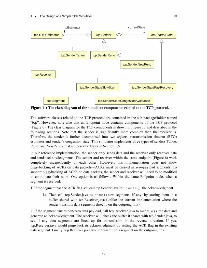
Figure 11: The class diagram of the simulator components related to the TCP protocol.

The software classes related to the TCP protocol are contained in the sub-package/folder named “tcp”. However, note also that an Endpoint node contains components of the TCP protocol (Figure 6). The class diagram for the TCP components is shown in Figure 11 and described in the following sections. Note that the sender is significantly more complex than the receiver is. Therefore, the sender is further decomposed into two objects: retransmission timeout (RTO) estimator and sender’s congestion state. This simulator implements three types of senders Tahoe, Reno, and NewReno), that are described later in Section 1.5.

In our reference implementation, the sender only sends data and the receiver only receives data and sends acknowledgments. The sender and receiver within the same endpoint (Figure 6) work completely independently of each other. However, this implementation does not allow piggybacking of ACKs on data packets—ACKs must be carried in zero-payload segments. To support piggybacking of ACKs on data packets, the sender and receiver will need to be modified to coordinate their work. One option is as follows. Within the same Endpoint node, when a segment is received:

1. If the segment has the ACK flag set, call tcp.Sender.java to handle() the acknowledgment

1a. Then call tcp.Sender.java to send()new segments, if any, by storing them in a buffer shared with tcp.Receiver.java (unlike the current implementation where the sender transmits data segments directly on the outgoing link).

2. If the segment carries non-zero data payload, call tcp.Receiver.java to handle() the data and generate an acknowledgment. The receiver will check the buffer it shares with tcp.Sender.java, to see if any data segments are lined up for transmission in the reverse direction. If yes, tcp.Receiver.java would piggyback its acknowledgment by setting the ACK flag in the existing data segment. Finally, tcp.Receiver.java would transmit this segment on the outgoing link.


20

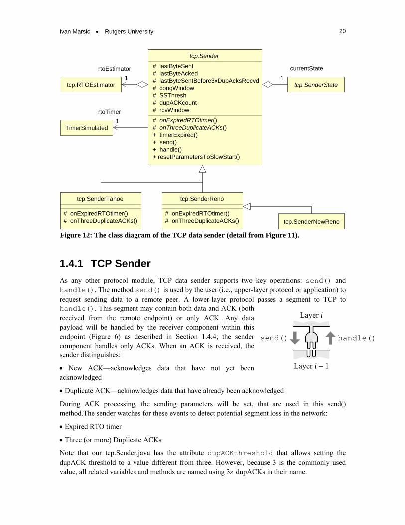
tcp.Sender

# lastByteSent# lastByteAcked# lastByteSentBefore3xDupAcksRecvd# congWindow# SSThresh# dupACKcount# rcvWindow

# onExpiredRTOtimer()# onThreeDuplicateACKs()+ timerExpired()+ send()+ handle()+ resetParametersToSlowStart()

tcp.Sender

# lastByteSent# lastByteAcked# lastByteSentBefore3xDupAcksRecvd# congWindow# SSThresh# dupACKcount# rcvWindow

# onExpiredRTOtimer()# onThreeDuplicateACKs()+ timerExpired()+ send()+ handle()+ resetParametersToSlowStart()

tcp.SenderTahoe

# onExpiredRTOtimer()# onThreeDuplicateACKs()

tcp.SenderTahoe


currentState

1tcp.SenderStatetcp.RTOEstimator

1

rtoEstimator

tcp.SenderReno


tcp.SenderReno

# onExpiredRTOtimer()# onThreeDuplicateACKs() tcp.SenderNewReno

TimerSimulated1

rtoTimer

Figure 12: The class diagram of the TCP data sender (detail from Figure 11).

1.4.1 TCP Sender

As any other protocol module, TCP data sender supports two key operations: send() and handle(). The method send() is used by the user (i.e., upper-layer protocol or application) to request sending data to a remote peer. A lower-layer protocol passes a segment to TCP to handle(). This segment may contain both data and ACK (both received from the remote endpoint) or only ACK. Any data payload will be handled by the receiver component within this endpoint (Figure 6) as described in Section 1.4.4; the sender component handles only ACKs. When an ACK is received, the sender distinguishes:

New ACK—acknowledges data that have not yet been acknowledged

Duplicate ACK—acknowledges data that have already been acknowledged

During ACK processing, the sending parameters will be set, that are used in this send() method.The sender watches for these events to detect potential segment loss in the network:

Expired RTO timer

Three (or more) Duplicate ACKs

Note that our tcp.Sender.java has the attribute dupACKthreshold that allows setting the dupACK threshold to a value different from three. However, because 3 is the commonly used value, all related variables and methods are named using 3 dupACKs in their name.

Layer i

Layer i 1

send() handle()


21

21

When the sender detects one of the above events, it simply delegates the event processing to its current state object. TCP sender operates the same send() regardless of its current state. The sender state is used in handle() to process the acknowledgment segments from the receiver. The state object (described in Section 1.4.2) performs the appropriate processing and returns the next state to which the sender should transition. This next state will become the sender’s current state.

Table 1: Operations of the class tcp.Sender.java:

Method Description

send() Sends segments by passing them to the network layer protocol.

handle() Processes ACKs received from the receiver. Checks for duplicate ACKs and dispatches them differently for processing.

ABSTRACT METHODS (to be implemented by the derived classes):

onExpiredRTOtimer()

Helper method, called on the expired retransmission timeout (RTO) timer from the sender’s current state object , see tcp.SenderState.handleRTOtimeout(). This method works slightly differently for different types of TCP senders (Tahoe, Reno, etc.).

onThreeDuplicateACKs() Helper method, called on three or more duplicate ACKs. Works differently for different types of TCP senders (Tahoe, Reno, etc.).

Figure 12 shows a detailed class diagram for the TCP sender; also see method description in Table 1. Note that the class tcp.Sender.java is an abstract class, which means that we cannot instantiate objects of this class. Instead, this class is completed by specific version of TCP sender (Tahoe, Reno, or NewReno), as shown in Figure 12. The two methods that are implemented by the derived concrete classes, onExpiredRTOtimer() and onThreeDuplicateACKs(), are specific to the concrete versions of a sender. We know that different sender versions behave differently when they detect segment loss based on three duplicate ACKs or RTO timer timeout.

The attributes of the sender (Figure 12) are fairly self-explanatory; also see detailed description in the book on the same website. The attribute lastByteSentBefore3xDupAcksRecvd is the pointer to the last byte sent (attribute lastByteSent) at the time when three duplicate acknowledgments were received. Only when all the data outstanding at that moment are acknowledged will the sender have fully recovered from the loss. The default value of this attribute is 1. This attribute is particularly used in TCP NewReno to distinguish “partial” from “full” acknowledgments (Section 1.5.3).

The class tcp.SenderNewReno.java is derived from the class tcp.SenderReno.java. The NewReno class is practically empty and its only purpose is to let the fast recovery state object decide how to process a new acknowledgment. For details, see the method calcCongWinAfterNewAck() in the class tcp.SenderStateFastRecovery.java.

1.4.2 Sender States

The class diagram for TCP sender states is shown Figure 13 and the methods are described in Table 2. We implement sender states using the state design pattern


22

tcp.SenderState

# calcCongWinAfterNewAck()# lookupNextStateAfterNewAck()+ handleNewACK()+ handleDupACK()+ handleRTOtimeout()

tcp.SenderState

# calcCongWinAfterNewAck()# lookupNextStateAfterNewAck()+ handleNewACK()+ handleDupACK()+ handleRTOtimeout()

tcp.SenderStateSlowStart

# calcCongWinAfterNewAck()# lookupNextStateAfterNewAck()

tcp.SenderStateSlowStart


tcp.Sender1

currentState

tcp.SenderNewReno





tcp.SenderStateFastRecovery

# firstPartialACK : boolean

# calcCongWinAfterNewAck()# lookupNextStateAfterNewAck()+ handleDupACK()

tcp.SenderStateFastRecovery

# firstPartialACK : boolean

# calcCongWinAfterNewAck()# lookupNextStateAfterNewAck()+ handleDupACK()

Figure 13: The class diagram of the states of TCP data sender (detail from Figure 11).

(http://en.wikipedia.org/wiki/State_pattern). The class tcp.Sender.java is the “context” object for which the state is extracted in the object of class tcp.SenderState.java. This means that the context object itself does not process any events, but rather passes the events on to its current state object for processing. The current state object processes the event and returns to the context object the next state it should transition to after this event. This next state becomes the new current state of the context object.

When the sender transitions to the Slow Start state (implemented by tcp.SenderStateSlowStart.java), this object should check that all congestion parameters are reset to their initial values. However, ours current implementation assumes that the object which initiated the transition has correctly reset the parameters and tcp.SenderStateSlowStart does not check that it is indeed so. To avoid multiple locations for resetting the parameters, tcp.Sender provides the method resetParametersToSlowStart() to do reset in a single place.

Note that the class tcp.SenderState.java is an abstract class, which means that we cannot instantiate objects of this class. Instead, this class is completed by specific state classes, as shown in Figure 13. The two methods that are implemented by the derived concrete classes, calcCongWinAfterNewAck() and lookupNextStateAfterNewAck(), are specific to the concrete state. We know from the TCP protocol standard that the sender’s congestion window size is calculated differently in the slow start state as opposed to the congestion avoidance state. The reader should examine the Java source code for the exact details.


23

23

Table 2: Operations of the class tcp.SenderState.java:

Method Description

handleNewACK()

Processes a single new (i.e., not duplicate) acknowledgment segment in the slow start transmission mode. Update the running estimate of the RTO timer interval. Restart the RTO timer for any outstanding segments. Update the congestion window size. Return the next state to which the sender will transition.

handleDupACK()

Counts a duplicate ACK and checks if the count equals 3. If exactly three dupACKs are received, it performs the fast retransmit and updates the congestion parameters. Tahoe ignores additional dupACKs over and above the first three. Reno does not—it processes them within its fast recovery procedure.

handleRTOtimeout()

Processes the TCP sender reaction to a retransmission timer (RTO) timeout. Method called on the expired RTO timer. After this kind of an event, the next state in any type of a TCP sender is always reset to slow start.

ABSTRACT METHODS (to be implemented by the derived classes):

calcCongWinAfterNewAck()

Helper method to calculate the new value of the congestion window after a "new ACK" is received that acknowledges data never acknowledged before. This method also resets the RTO timer for any outstanding segments.

lookupNextStateAfterNewAck() Helper method to look-up the next state that the sender will transition to after it received a "new ACK".

Note that the class tcp.SenderStateFastRecovery overrides the method handleDupACK() of its base class tcp.SenderState. In the fast-recovery state, the TCP Reno sender for each dupACK increases the congestion window by one full MSS. This action inflates the congestion window for the additional segment that has left the network. The sender remains in the state of fast recovery until it receives a new ACK that acknowledges previously unacknowledged data. More discussion of TCP Reno is available in Section 1.5.2 of this document, as well as in the book.

An important note about the method handleNewACK() in SenderState.java: For simplicity, our TCP Receiver is allowed to send cumulative acknowledgements for more than two segments that arrived in order—the number is unlimited. In reality, the delayed ACK timer (Section 1.2.2) will expire relatively soon and a cumulative ACK will acknowledge up to two segments. Our simplification can cause a problem in that the retransmission interval (Section 1.4.3) may not converge quickly enough to its true value because of the severely reduced number of new acknowledgements that trigger the retransmission interval re-estimation. For this reason, the method handleNewACK()calls the method updateRTT() of RTOEstimator.java as many times as the number of segments cumulatively acknowledged by a new acknowledgement.

Another issue is counting and handling duplicate acknowledgements in the method handleDupACK(). The attribute dupACKcount of tcp.Sender.java (Figure 12) holds the current tally of duplicate ACKs. This attribute must be rest when an acknowledgement for new data is received (see the definition of “new data” in Section 1.4.3). When three duplicate ACKs


24

are received, the method handleDupACK() calls the sender’s onThreeDuplicateACKs(), which is specific to the running version of the sender. Tahoe ignores additional dupACKs over and above the first three. Reno does not—it processes them within its fast recovery procedure. An important issue is where to reset the attribute dupACKcount. We cannot reset it in the method onThreeDuplicateACKs() after three dupACKs, because six or more may arrive consecutively and for every modulo three number of dupACKs, onThreeDuplicateACKs() would mistakenly adjust the congestion parameters, such as reduce SSThresh. The proper approach is to detect an acknowledgement for new data and reset it then, which occurs in SenderState.handleNewACK(). Reno and its derivative NewReno maintain the attribute lastByteSentBefore3xDupAcksRecvd (Figure 12) to detect a “true” new ACK, while for Tahoe we take a simplified approach and reset dupACKcount for any ACK that acknowledges previously unacknowledged data.

1.4.3 Timeout Interval Estimation

Whenever data are sent on a connection, the retransmission timeout (RTO) timer is started, unless it is already running. TCP sender runs a single RTO timer for all outstanding segments. When all outstanding data are acknowledged, the timer is stopped. If the timer expires, the oldest unacknowledged segment is retransmitted and the timer is restarted with a double value (this behavior is known as “exponential backoff”).

Timeout interval estimation is performed continuously by the object tcp.RTOEstimator.java. TCP maintains two smoothed estimators per connection: the round-trip time (RTT) and the mean deviation of the RTT. These estimators are represented respectively with the attributes estimatedRTT (current estimated RTT value) and devRTT (current estimated RTT deviation). These estimators are maintained as scaled integer numbers to provide adequate precision without using floating-point code within the operating system kernel. Following this approach, our implementation uses shift operations instead of multiplication and division.

Note that the same estimated value is used for idle-connection timers as well (Section 1.2.2).

This implementation is based on RFC-6298 and TCP/IP Illustrated, Volume 1 [Stevens, 1994: Chapter 21]. TCP sender maintains a single retransmission timeout (RTO) timer, named rtoTimer (see Figure 3 and Figure 12). RTO timer value is measured in simulator time ticks that are defined by the method Simulator.getTimeIncrement(). The timer is activated when a new segment is transmitted. When all outstanding segments are acknowledged, the timer is deactivated.

The sending time of each TCP segment is recorded as tcp.Segment.timestamp in the TCP header (similar to the timestamp option in the Options field of an actual TCP header) and returned by the corresponding acknowledgment packet. tcp.Segment.timestamp is set to 1 if the segment is a retransmitted segment, and no RTT estimation is performed for retransmitted segments.

SampleRTT = current_time timestamp;

EstimatedRTT[new] = (1 )EstimatedRTT[old] + SampleRTT;

Delta = |SampleRTT EstimatedRTT[old]|;


25

25

DeviationRTT[new] = (1 )DeviationRTT[old] + Delta;

The above computation should be performed using =1/8 and =1/4. An exception occurs when the first RTT measurement is made, where the host must set:

SampleRTT = current_time timestamp;

EstimatedRTT[new] = SampleRTT;

DeviationRTT[new] = SampleRTT / 2;

The retransmission timer base is always computed as:

TimeoutInterval[new] = EstimatedRTT[new] + max{ G, KDeviationRTT[new] }.

where G is the system clock granularity (in seconds), and K is usually set to 4. (Check RFC-6298 for discussion about the need for the clock granularity parameter G.)

The “exponential backoff” behavior may lead to very large values for RTO timeouts. RFC-6298 (Section 5) states that a maximum value may be used to provide an upper bound to this doubling operation. This website says that the retransmission timer should not exceed 240 seconds: https://support.microsoft.com/kb/170359/en-us.

Restarting the RTO Timer

According to RFC-2988, Step 5.1, [Paxson & Allman, 2000], every time a packet containing data is sent (including a retransmission), if the timer is not running, start it running so that it will expire after RTO seconds (for the current value of RTO).

An interesting issue is about re-starting the retransmit timer. TCP sender re-starts the RTO timer when a new acknowledgment (acknowledges data never before acknowledged) is received and there are still outstanding, non-acknowledged segments. There are three cases of new ACKs:

1. The sender has received a non-duplicate ACK and is currently sending new data (either in slow start or congestion avoidance) and is not aware of any data loss. When the sender transmits the EffectiveWindow amount of data, it re-starts the rtoTimer.

2. The sender has received a non-duplicate ACK after receiving three or more duplicate ACKs and retransmitting one or more unacknowledged segments. Different sender versions react differently. Tahoe and Reno will re-set the retransmit timer if there are still outstanding segments. NewReno distinguishes “old data” as any data that has been unacknowledged at the time when a segment loss was detected, and “new data” as the data that is sent after the loss was detected. A non-duplicate ACK for “old data” may acknowledge the old data only partially or completely (see Section 1.5.3). Different approaches for reacting to a “partial ACK” in NewReno were considered by Floyd et al. (2004). The so-called Impatient variant resets the retransmit timer only after the first partial ACK. Our simulator implementation adopted the so-called Slow-but-Steady variant in which the retransmit timer is reset after each partial acknowledgement, because it performs better in our simulation scenarios. Therefore, although the class SenderStateFastRecovery.java has the attribute firstPartialACK (Figure 13), we are currently not using it. See the implementation details in the method calcCongWinAfterNewAck().


26

3. The sender has received a non-duplicate ACK after the retransmit timer expired and the sender retransmitted the oldest unacknowledged segment. Assuming that there are still outstanding segments, it is not clear if the RTO timer should be re-started again, because it was restarted just after it expired.

I could not find a definite answer to the last/third case, so the sender will re-start the RTO timer twice in a row (after it expired and when the new ACK is received for the retransmitted segment). Because this may introduce an unnecessary inefficiency, I feel that this issue is unresolved and needs to be revisited. Any modifications should be made in the method calcCongWinAfterNewAck() of the classes SenderStateSlowStart,java and SenderStateCongestionAvoidance.java.

Additional information about retransmission timers and approaches for providing faster loss recovery is available in [Hurtig et al., 2014].

1.4.4 TCP Receiver

TCP Receiver is implemented by the class tcp.Receiver.java.

If a segment arrives with an invalid checksum, TCP silently discards it and does not acknowledge receiving it. There is no means for negatively acknowledging a segment. The receiver expects the sender to time out and retransmit. The receiver does not know what to do with a corrupted packet—it does not even know if this packet was intended for this receiver, because corrupted bits might have caused a delivery to a wrong destination. In our implementation, the class Packet.java has the Boolean attribute inError, which serves in lieu of error checksum.

An out-of-order packet must be acknowledged immediately by a duplicate ACK. However, for in-order packets a cumulative ACK will be maintained, indicating the TCP receiver has received all of the data up to the indicated byte. A cumulative ACK will be sent only when a timer expires. The timer for delayed (cumulative) acknowledgments is called delayedACKtimer (Figure 3).

There are two standard methods that can be used by TCP receivers to generate acknowledgments. The method outlined in RFC-793 generates an ACK for each incoming data segment (including in-order segments). RFC-1122 states that hosts should use “delayed acknowledgments” for in-order segments. Using this approach, an ACK is generated for at least every second in-order, full-sized segment, or if a second full-sized segment does not arrive within a given timeout (which must not exceed 500 ms [RFC-1122], and is typically less than 200 ms). Such approach is also adopted in RFC-2581. RFC-2581 states that an ACK should be generated for at least every second full-sized segment, and must be generated within 500 ms of the arrival of the first unacknowledged packet. Therefore, the receiver can send an ACK for no more than two data packets arriving in-order.

RFC-2760 also allows for generating “Stretch ACKs” that acknowledge more than two in-order full-sized segments. This approach provides a possible mitigation, which reduces the rate at which ACKs are returned by the receiver. Interested readers should check for discussion of modified delayed ACKs in Section 4.1 of RFC-3449. The way cumulative ACKs are implemented by our tcp.Receiver.java they should probably be called “Stretch ACKs,” because we generate a single cumulative ACK for all in-order segments received during a single transmission round.


27

27

// if pkt arrived in-sequence:

process()

handle(pkt)

: Simulator receiverEndpt : Endpoint : Receiver

run()

link2 : Link

process()

deliverArrivedPackets()

handle(pkt)

set cumulative ACK

start delayed ACK timer

setTimeoutAt( current iteration )

checkExpiredTimers()sendCumulativeAcknowledgement()timerExpired()

Figure 14: Sequence diagram for generation and sending of cumulative ACKs.

Because our time is measured in unspecified clock ticks and it is of very coarse granularity (one tick corresponds to one RTT), the Receiver sets the delayed-ACK timer to the current time. Here we use the knowledge of how the simulator works. We know that ACKs will be generated during the call to the Receiver’s method handle(), which is called by the incoming Link (Figure 14). In effect, we are starting the delayed-ACK timer to expire during the same simulation round, which in our case corresponds to one RTT, at the time when process() on the receiving endpoint will be called.

There is also a TCP standard that supports selective acknowledgment (SACK). A selective acknowledgment option allows receivers to additionally report non-sequential data they have received. SACK is not implemented in our reference implementation. For details, see RFC-2018 [Mathis, et al., 1996].

1.5 Supported Versions of TCP

A number of TCP variants have been proposed and studies. The current code implements these versions of the TCP sender: Tahoe, Reno, and NewReno. TCP receiver is universal and does not depend on the TCP sender version. This code does not implement TCP Selective


28

Acknowledgment Options (SACK), described in RFC-2018. Different RFCs can be found here http://tools.ietf.org/rfc/index.

Early TCP implementations in early 1980s followed a Go-back-N model using cumulative positive acknowledgment and requiring a retransmit timer expiration to resend data lost during transport. These TCPs did little to minimize network congestion. The Tahoe TCP implementation [Jacobson, 1988] added a number of new algorithms and refinements to earlier implementations. These algorithms are present in most modern TCP versions, along with additional refinements and algorithms. Therefore, it is a good strategy to start with studying TCP Tahoe and progress incrementally towards more modern TCP versions.

1.5.1 TCP Tahoe

TCP Tahoe was developed in the late 1980s. Our simulator implementation is based on RFC-1122 (http://www.apps.ietf.org/rfc/rfc1122.html): “Requirements for Internet Hosts -- Communication Layers,” published in 1989, which I believe specified TCP Tahoe. See Section 4.2 of RFC-1122.

TCP Tahoe includes the algorithms for Slow Start, Congestion Avoidance, and Fast Retransmit. In our implementation, Slow Start and Congestion Avoidance are implemented as sender states (Section 1.4.2), and Fast Retransmit is implemented as an action when the sender suspects a segment loss. With Fast Retransmit, after receiving a small number (usually 3) of duplicate acknowledgments for the same TCP segment (dup ACKs), the sender infers that a segment has been lost and retransmits the segment without waiting for a retransmission timer to expire. This behavior leads to higher channel utilization and connection throughput. The Fast Retransmit algorithm is slightly modified in subsequent versions of TCP, as described in Section 1.5.2.

As shown in Figure 12, the Tahoe sender is implemented by the class tcp.SenderTahoe.java derived from the base class tcp.Sender.java. The method onExpiredRTOtimer() resets the sender’s congestion-control parameters when the RTO timer times out. The sender begins again ramping up its congestion window in the slow start state.

The method onThreeDuplicateACKs() performs the Fast Retransmit action to retransmit the oldest outstanding segment because after three dupACKs, it is presumably lost. In the class tcp.Sender.java, the threshold for the number of duplicate ACKs is called dupACKthreshold, and is by default set to three, but this value can be modified. The Tahoe sender does not care about the number of dup ACKs as long as it is at least three (or whatever value dupACKthreshold is set to). This means that any dupACKs received after the first three are ignored. Also, after this kinds of an event, the sending mode in TCP Tahoe is always reset to slow start. The method leaves the RTO timer running for the outstanding segments.

All other operational logic of the sender is delegated to the sender states (Section 1.4.2), and Tahoe has only two states: Slow Start and Congestion Avoidance.

TCP Tahoe was superseded by TCP Reno, which is described next.

1.5.2 TCP Reno

TCP Reno is designed to address a common case of single segment loss, when after the Fast Retransmit, the communication path (“pipe”) becomes empty and the Tahoe sender labors to re-


29

29

fill the pipe in the Slow Start state. The TCP Reno retained the basic features of TCP Tahoe (Section 1.5.1), but the key difference is that the Fast Retransmit is modified to include Fast Recovery [Jacobson, 1990]. Reno implementation of a sender that appeared first in early 1990s. TCP Reno was specified in RFC-2001 (http://www.apps.ietf.org/rfc/rfc2001.html) and RFC-2581 (http://www.apps.ietf.org/rfc/rfc2581.html).

Fast Recovery is entered by a TCP sender after receiving an initial threshold of duplicate ACKs, generally set as dupACKthreshold = 3. Once three dup ACKs are received, the sender retransmits the oldest unacknowledged segment and reduces its congestion window by one half. Instead of repeating slow starting, as done by a Tahoe sender, the Reno sender uses additional incoming dup ACKs to clock subsequent outgoing segments.

In Reno, the sender’s usable window is calculated as follows.

For dupACKcount dupACKthreshold:

EffectiveWindow = min(RcvWindow, CongWindow)

For dupACKcount dupACKthreshold:

EffectiveWindow = min(RcvWindow, CongWindow+ dupACKcount)

where RcvWindow is the receiver’s advertised window, CongWindow is the sender’s congestion window, and dupACKcount counts the number of duplicate ACKs. Thus, during Fast Recovery the sender “inflates” its window by the number of dup ACKs it has received, based on the observation that each duplicate ACK indicates a packet has left the network and is now cached at the receiver. After entering Fast Recovery and retransmitting the oldest unacknowledged segment, the sender effectively waits until half a window of dup ACKs have been received, and then sends a new segment for each additional dup ACK that is received. Upon receipt of an ACK for new data (called a “recovery ACK”), the sender exits Fast Recovery, sets dupACKcount to 0, and enters Congestion Avoidance.

Reno significantly improved upon the behavior of Tahoe when a single segment is dropped from a window of data. However, even Reno can suffer from performance problems in case of a “catastrophic loss” when multiple segments are dropped from a window of data. This is illustrated in the simulations for our default configuration, when several segments are dropped for a Reno connection with a large congestion window after slow-starting in a network with drop-tail routers (Section 1.3.2). As a result, the sender needs to await a retransmission timer expiration before reinitiating data flow. To address such cases, TCP NewReno modification was introduced.

1.5.3 TCP NewReno

The current version of TCP is called “NewReno” and specified in RFC-5681 (http://tools.ietf.org/html/rfc5681). This is a modified version of TCP Reno that avoids some of the performance problems when multiple segments are dropped from a window of data (see Section 1.5.2). Our NewReno implementation includes a small change to the Reno algorithm that eliminates Reno’s wait for a retransmit timer when multiple segments are lost from a window. The change affects the sender’s behavior during Fast Recovery when a “partial ACK” is received that acknowledges some but not all of the segments that were outstanding at the start of that Fast Recovery period (represented by the attribute lastByteSentBefore3xDupAcksRecvd,


30

see Section 1.4.1). In the ordinary Reno, a partial ACK will take TCP out of Fast Recovery into the Congestion Avoidance state. In NewReno, partial ACKs received during Fast Recovery are treated as an indication that the segment immediately following the acknowledged segment in the sequence space has been lost, and should be retransmitted. Thus, when multiple segments are lost from a single window of data, NewReno can recover without a retransmission timeout, retransmitting one lost segment per round-trip time until all of the lost segments from that window have been retransmitted. NewReno remains in Fast Recovery until all of the data outstanding when Fast Recovery was initiated have been acknowledged. This is known as a “full ACK” received, and at this time, lastByteAcked becomes equal to lastByteSentBefore3xDupAcksRecvd.

Our class tcp.SenderNewReno.java derived from the base class tcp.SenderReno.java (Figure 12), but the class does nothing. It only serves as a type indicator for tcp.SenderStateFastRecovery.java to know in which context it is running (old Reno or NewReno) and to behave accordingly. See the method calcCongWinAfterNewAck() of tcp.SenderStateFastRecovery.java for details.

RFC 5681 (in Section 3.2) states that the retransmit timer should be reset only for the first partial ACK that arrives during fast recovery. Timer management is discussed in more detail in Section 4 of RFC 5681. Our simplified implementation resets the RTO timer for every partial ACK. See the method handleNewACK() of the class SenderState.java.

31

Contents 2.1 Assignment 1: Unlimited Queue and Bandwidth Bottleneck

2.1.1 Software Modification Description 2.1.2 Experiment Description

2.2 Assignment 2: Packet Reordering During Transit


2.3 Assignment 3: Variable Occupancy of the Router Buffer


2.4 Assignment 4: Concurrent TCP and UDP Flows


2.5 Assignment 5: Competing TCP Flows and Fairness


2.6 Assignment 6: Active Queue Management Policy


2 Programming Assignments

The programming assignments described in this section are intended to explore a wide variety of “what if” questions about the real-world systems using TCP protocol. The students will simulate potential changes to the default network configuration and predict their impact on system performance. These assignments are based on Example 2.1 in the book (Section 2.2). They are mainly asking the student to modify the network properties (represented by the classes Simulator.java and Router.java) and observe the effect on TCP performance.

The following assignments are designed to illustrate how a simple model can allow studying individual aspects of a complex system. In this case, we study the congestion control in TCP. The students are asked to modify the program code, run the experiments, and interpret the simulation results. All of these projects require only relatively simple extra coding because most of the code is already written. The main focus is on running thoughtful experiments and performing extensive analysis and explanation of the observed results.

The assignments are based on the reference software implementation available at this book’s web site; follow the link “Team Projects.”

All assignments are structured as follows:

1. Problem Formulation states the problem to be studied and questions to be answered by simulation. The overall project plan is also summarized.

2. Model Conceptualization and Software Modification describes a model of the system to study. As noted, the assignments mostly ask the student to modify the network properties (represented by the classes Simulator.java and Router.java).

3. Experimental Design, Data Collection and Interpretation describes the experiments to perform and the kind of data to be collected, mostly samples of TCP congestion parameter values. The student must know what kind of data to expect, so to verify that the input parameters and logical structure of then model are correctly represented in their software implementation.


32

4. Documentation and Reporting included the documentation of the program modifications in Step 2 above, as well as experiments and results interpretation in Step 3 above. When documenting your program modifications, describe only what modifications you introduced relative to the reference implementation described in Section 1 of this document. In the discussion of the results, plot the relevant charts similar to those provided for Example 2.1. Calculate the sender utilization, where applicable, and provide explanations and comments on the system performance. Also, calculate the latency for transmitting a very large file. The result of all the analysis should be reported clearly and concisely. Good documentation will add to the credibility of your modified model and your experimental results.

Each chart/table should have a caption and the results should be discussed. Explain any results that you find non-obvious or surprising. Use manually drawn diagrams (using a graphics program such as PowerPoint), similar to figures in Section 2.2.1 of the book, where necessary to support your arguments and explain the detailed behavior.

Important Notes:

● The data size for bulk transport is set in the parameter TOTAL_DATA_LENGTH, in the class Simulator.java, which is by default set to 1,000,000 bytes. When experimenting with bulk data transfer and large number of iterations (order of thousands), ensure that the sender has unlimited data ready to send. If the sender runs out of data, you will receive this message: tcp.Sender.send(): Insufficient data to send

● Run the simulations for short and long sessions. Short sessions of about 100 iterations will illustrate the transient behavior (sporadic and short bursts of data). Long sessions with large number of iterations (at least 1000 iterations), will illustrate the steady-state behavior.

● Sender utilization is defined as the fraction of time the sender is busy transmitting packets relative to the duration of the entire session. It is desirable that the sender is more utilized rather than sitting idle (of course, this is assuming that it has packets ready for transmission; otherwise it has no choice but to sit idle and wait for new packets).

● When comparing different sender versions (Tahoe, Reno, NewReno) on their transient behavior, use a relatively small TOTAL_DATA_LENGTH (order of KBytes to tens or hundreds or KBytes) and determine the number of iterations each sender needs successfully to complete the transmission.

● When comparing different sender versions on their steady-state behavior, use a very large TOTAL_DATA_LENGTH (order of hundreds of MBytes or GBytes) and determine the sender utilization for each version over a large number of iterations (order of thousands). Here we want to know how much data each sender version is able to push into the network for a fixed number of iterations, given unlimited data to send.


33

2.1 Assignment 1: Unlimited Queue and Bandwidth Bottleneck

This assignment considers the TCP behavior when the network configuration remains the same as in Figure 4, but the router has practically unlimited memory capacity, say 10,000 packets. Due to the large router buffer size there will be no packet loss, but the bandwidth mismatch between the router’s input and output links still remains. Therefore, packets may experience large delays. Our goal is to study the router queue length over time and the delays experienced by the packets. We would like also to see whether these delays affect the sender utilization. Finally, we are interested to see if the sender may mistake a large queuing delay for packet loss.

2.1.1 Software Modification Description

We assume that, as in the reference implementation, the sender receives a cumulative ACK for all segments transmitted in one transmission round. After sending the number of segments limited by its effective window size, the sender must wait for at least one round-trip time for an acknowledgment to arrive. To calculate the maximum number of segments that the sender can send before an ACK arrives, we need to know how long is the RTT. The network configuration in

Router Receiver

ACKACK

RTT

RTT

N packetstransmittedon Link-2per RTT

Link-2 (1 Mbps)

N/2 packetsack-ed fromprevious round

+N/2 packetsack-ed fromthis roundper RTT

Sender Link-1 (10 Mbps)

ACKACK

N packetstransmittedon Link-1per RTT

Figure 15: The time diagram for Assignment 1 that illustrates how the number of packets transmitted in one round is limited by the bandwidth of Link-2.


34

ACKACK

ACKACK

RTT

Figure 4 provides the link data rates, but not lengths. Therefore, let us assume that RTT = 0.5 seconds. We also set RcvWindow = 1 MByte instead of the default value of 65535 bytes, to avoid having the receive window limit the number of segments to be sent in one round.

Because of the 10 : 1 bandwidth mismatch between the router’s input and output links, the router may not manage to relay all the packets from the current round before the arrival of the packets from the subsequent round. This behavior is illustrated in Figure 15 (and also in the inset figure on the right, which illustrates how the pattern repeats for each RTT). As shown in Figure 15, because the first link is much faster, the sender transmits the effective window of packets quickly and then waits idle for an acknowledgment. The packets that the router is not able to transmit in the current round are carried over to the next round and they accumulate in the router’s queue. As the sender’s congestion window size grows, there will be a queue buildup at the router. There will be no loss because of the large buffer size, but packets may experience delays. Because of the first-come-first-served policy, the packets carried over from a previous round will be sent first, ahead of the newly arrived packets. The queuing delays may trigger the sender’s RTO timer before the packets propagate to the receiver and their ACKs arrive to the sender.

The key code modifications are to the router code (see Figure 8 in this document). For example, we need to increase the capacity (attribute bufferCapacity) of the router memory, represented by the array packetBuffer[]. The experimental data (described next) can be captured in the method Router.process().

The TCP sender utilization that is reported at the end of method run() in Simulator.java may not be appropriate for this experimental scenario. Because the router buffer is large, the maximum possible number of transmitted packets may be limited by the datarate of the first link (Figure 4). Given that in our case R1 = 10 Mbps and sender’s maximum segment size (MSS) is 1024 bytes, this sender will not be able to send more than 107 / (1024 8) = 1,220 segments per second.

2.1.2 Experiment Description

Run the experiment for all three TCP versions (Tahoe, Reno, and NewReno). Determine the following:

1. Determine whether the system stabilizes, i.e., whether the congestion window size saturates and plateaus or it keeps growing. Run the simulations for large number of iterations, say at least 1000 iterations, to reach a steady state.

2. Determine whether the router buffer occupancy will ever reach its total capacity.

3. Calculate the average queuing delay per packet, i.e., the average number of rounds that a packet will be waiting for transmission on Link 2.

4. Are there any packet retransmissions (quantify, how many) due to large delays (although packets are never lost)? Explain your answer using manually drawn diagrams to support your arguments.

In addition to the regular charts for congestion parameters, plot the charts shown in Figure 16. The chart on the left should show the number of the packets that remain buffered in the router at the end of each transmission round. (This number should not include the packets that the router


35

Time

[in RTT units]0 1 2 3 4

Number of packets left unsent in the router buffer at the end of each transmission round

Average delay for packets transmitted in a given round

Time


Waiting time


Distribution of packets over the entire simulation that waited in the router buffer for a given

number of transmission roundsNumber of

packets that spent zero RTT in router

buffer

Number of packets that spent 1RTT in router buffer Number of packets that

spent 2RTT in router buffer

Figure 16: Results charts for Assignment 1.

transmitted on the outgoing link during this round.) Note that the time axis is shown in RTT units. The chart on the right shows the average delay for packets transmitted in a given round. The delay includes the transit time and queuing time. The transit time comprises transmission and propagation times and in case of no queuing at the router, the transit delay is ½RTT. When packets remain queued in the router and are forwarded in a future round, we add one RTT to the packet’s delay for each round that it spends in the router memory. Provide explanation for any surprising observations or anomalies.

In addition to the above charts, you should investigate the following problem. While a long queue is less likely to overflow during a traffic burst (thus reducing packet loss probability), it potentially increases the queuing delay for non-dropped packets. A short queue reduces this delay, but conversely increases the probability of packet loss for bursty traffic. Experiment by adjusting the router buffer size and determine what values minimize both packet loss and queuing delays. Plot a chart to illustrate your results.

2.2 Assignment 2: Packet Reordering During Transit

In the reference example implementation, the packet transit times are clocked to the integer multiples of RTT. For example, packets #2 and 3 travel together during the round = 2 RTT; packets #4, 5, 6, and 7 travel together during the round = 3 RTT; and so on. In addition, duplicate ACKs are generated only because of packets dropped in the router, never because of reordered packets. This idealization may not reflect the reality. This assignment explores what


36

happens when packets are reordered during transit (rather than only dropped). The router will hold packets for several RTT units to simulate packet-reordering delays when different packets travel along different routes. An in-depth analysis of effects of packet reordering on TCP is available in [Leung, et al., 2007].


One way to implement this modification is explained next; the reader is encouraged to search for better or alternative implementations. The key change in the code will in the class Router.java. First, we increase the router’s memory size to avoid dropping new packets because delayed packets are occupying the memory. Try with a relatively small increase, say to bufferCapacity = 15 packets, so that some new packets still may be dropped.

Second, to maintain the record of delays for individual packets, we add a new attribute to tcp.Segment.java ( public double delay = 0.0; ). This field will be used only by Router.java and will be ignored by all other classes.

Third, modify the method Router.handle() so that for every newly received packet, the router assigns an exponentially distributed random amount of delay (measured in integer number of round-trip times 0). For a new packet first check whether it will be dropped or queued in the array packetBuffer[]. If latter, generate an exponentially-distributed integer random number with and a small mean value, say 1 or 2, and a small variance. Set the delay attribute (introduced in the second step above) to the generated delay value. (The delay value must be an integer 0.)

To generate exponentially distributed random numbers, generate a uniformly distributed random number u on the unit interval [0, 1]. In Java, there is a method random() in the Math class, which returns a uniformly-distributed double value between 0.0 and 1.0. Then apply the following function to obtain an exponentially distributed random number rx:

uurx

ln)(

(Eq. 2)

where ln() is the natural logarithm (using basis e), 1/ is the mean value, and the variance is given by 1/2.

Fourth, modify the method Router.process() so that for every invocation, the router decrements all delays and transmits on the outgoing link only the packets for which the delay became to zero. Specifically, we iterate through the array packetBuffer[] and for each packet packetBuffer[i] reduce the delay value by the amount of time elapsed since the previous call to this method (represented by the attribute lastTimeProcessCalled). If the delay becomes zero after decremented, transmit the packet to the outgoing link.

Expose the relevant parameters (e.g., buffer capacity, and exponential distribution’s mean and variance) in the user interface, so to allow entering different values from the command line, similarly to entering other parameters for simulation (see Section 1.1.1 of this document).

Visit http://en.wikipedia.org/wiki/Exponential_distribution for information about exponential probability distributionVisit http://en.wikipedia.org/wiki/Exponential_distribution for information about exponential probability distribution


37


Note that if you run your simulation say for 100 iterations, there may at the end still remain some packets in the router in packetBuffer[], because their delay still has not reached zero. You will need to flush the router buffer by invoking Router.process() for several subsequent ticks of the simulation clock, until no packets remain in packetBuffer[].

Note that, unlike Example 2.1 in the book, where a TCP segment can arrive at the receiver out-of-sequence only because a previous segment was dropped at the router, in your assignment an additional reason for out-of-sequence segments is that different segments may experience different amounts of delay. Each packet is assigned the delay value individually, as generated by the random number generator. So if, say, three packets arrive at the router, then it is possible that packet #1 is delayed by 4, so it will have to sit inside the router buffer through four invocations of method Router.process(). On the other hand, packet #2 that arrived in the same iteration could get assigned delay 0 and leave at the end of this method invocation, and packet #3 could get assigned the delay value 1 and leave in the next invocation, but still before packet #1. Recall that for every out-of-order packet, the receiver reacts immediately and sends a duplicate acknowledgment (Section 1.4.4 of this document). Your simulation will show what happens when packets are reordered. By controlling the capacity of the packetBuffer[] array, you may also cause packets dropped because of the router buffer overflow when the buffer is holding the delayed packets.

Run the experiment for all three TCP versions (Tahoe, Reno, and NewReno). Run the simulations for large number of iterations (at least 1000), to ensure that the senders reach a steady state.

Print and visualize the relevant statistics from your new router code for every iteration, such as:

the number of packets over time that are currently delayed in packetBuffer[] after the method Router.process() is exited; show either the average delay per packet during each RTT, or cumulative delays for all packets transmitted during each RTT;

the histogram of delay values for packets currently left in packetBuffer[]; and,

how many packets are dropped because of the router buffer overflow.

Plot the congestion parameters, packet delays, and the number of dropped packets on the same timeline or two aligned timelines. Analyze whether there is any correlation (positive or negative) between the congestion parameters and packet delays and losses.

Based on experiments, answer what causes greater drop in the sender utilization: few packets significantly delayed, or large number of packets slightly delayed? Experiment with different percentages of delayed packets, starting with only 1% packets subject to random delays, and go in steps of 5% to 100% packets subject to random delays. Plot the sender utilization chart with different values of parameter for the exponential distribution in Eq. (2) and explain your experimental observations. Because of the randomness aspect of the experiment, average the results over multiple runs to obtain average sender utilization.

Note: Two effects may be confounded in this experiment: random delay and packet loss because of router buffer overflow. Our router simulates transit delays by holding packets in the buffer for a random time. However, this holding also interferes with new packets which may arrive to an full buffer. Keep in mind that this experiment is a simulation of reality—normally routers do not


38

deliberately hold packets to cause delays. To separate the effects of random delay and buffer overflow, you should consider implementing a separate memory for holding the delayed packets. Only the packets that are ready for transmission (assigned zero delay) should be placed in the regular buffer. Packets that are assigned a non-zero delay should be placed in the new buffer, and moved to the regular buffer only when they are ready for transmission. In this way, the deliberately delayed packets will avoid causing packet loss due to buffer overflow.

2.3 Assignment 3: Variable Occupancy of the Router Buffer

In our reference implementation, the available router buffer capacity is constant (e.g., 6 packets plus 1 in transmission, Figure 4). This assignment explores a more realistic scenario of variable buffer occupancy because of parallel flows (not necessarily TCP flows) that cross paths with our flow. The experimental scenario will still have a single TCP connection as in the reference implementation. The router will be modified to simulate random arrivals of packets on other intersecting flows. In each transmission round, the router will reduce the available memory capacity by a random amount generated according to an exponential distribution. We assume that all packets external to our TCP flow are of the same size as our packets (i.e., one packet fills one router buffer slot). All packets from other flows that “arrived” in one round are assumed to depart the router in the same round and a new random occupancy number will be generated in the next round. Our goal is to study TCP sender utilization under variable occupancy of the router buffer.

A more realistic simulation should consider introducing a “memory” property for router buffer occupancy. That is, packets from other flows that “arrived” in one round may not all depart the router in the same round—if a large number “arrived,” some may stay of one or more rounds. Some kind of dependency between router occupancy over time may be introduced.


The router will be modified to dynamically change its buffer size. We will keep the attribute bufferCapacity constant, and currentBufferOccupancy still represents the number of packets from our TCP connection that are currently buffered in the router. We also introduce an additional attribute called otherFlowsOccupancy, which is an integer number that represent how many packets from other flows occupy memory slots. This attribute is an exponentially-distributed random variable that takes the values from the range [0, bufferCapacity currentBufferOccupancy]. When a new packet arrives on the TCP flow, the router generates from this range a random value for otherFlowsOccupancy. Generating exponentially distributed numbers is described in Section 2.2.1 for Assignment 2. The router then applies the following rule:


39

CongWindow

EffctWindow

Time [in RTT]

Time [in RTT]

[Byt

es]

[Pac

kets

]

Average Number of Packets from Other Flows

Flight Size from Our Flow

Figure 17: Results chart for Assignment 3. The shown curves are not meant to represent the actual shape of the curves that will be found by experimentation.

IF currentBufferOccupancy otherFlowsOccupancy bufferCapacity, then queue the new packet in router’s memory and increment currentBufferOccupancy by one; ELSE discard the new packet;

If time permits, you should also implement sending sporadic bursts of data, as described in Section 2.4.1 for Assignment 4.


Run the experiment for all three TCP versions (Tahoe, Reno, and NewReno) and for large number of iterations, say at least 1000 iterations.

(a) Determine the sender utilization under a fixed buffer size, by setting different values for the attribute bufferCapacity. In addition to the default value of 6, try values ranging from 3 to 10, or greater.

(b) Determine the sender utilization under a variable buffer size, by setting different values for the parameter of exponential distribution, such that the mean value 1/ ranges between [1, bufferCapacity 1]. If the generated random number exceeds bufferCapacity, it must be truncated to bufferCapacity. Note that you should not use large values of 1/ because this would result in many truncations, thus significantly distorting the exponential distribution.

Compare the sender utilization for case (b) with that for case (a). Note that in case (b) when the mean value 1/ equals 1, then the router memory capacity is, on average, reduced by one packet. Compare this scenario to the scenario under case (a) where the router capacity is set fixed to bufferCapacity 1. Explain any observed difference in sender utilization under deterministic reduction of buffer capacity (case (a)) versus stochastic reduction of buffer capacity (case (b)). Compare also other corresponding scenarios for cases (a) and (b).

Perform the experiments for both transient behaviors (sending sporadic bursts of data), and steady-state behaviors (unlimited bulk-data transfer) Recall from the notes on page 32 that for


40

bulk transfers we want to know how much data each sender version is able to push into the network for a fixed number of iterations, given unlimited data to send. Run the simulations for large number of iterations (order of thousands), to ensure that the sender reaches a steady state.

Keep in mind that, because of the randomness involved, you cannot derive meaningful conclusions based on individual runs. Instead, repeat each experiment for tens of runs and take the average values of observed parameters.

Analyze whether there is any correlation (positive or negative) between the congestion parameters and buffer occupancy by concurrent flows (see Figure 17). It may be difficult to infer the dependencies by mere eye examination and a better approach is to calculate the correlation between different time series, such as between the effective window and the number of packets from other flows, or between the congestion window and the other packets. Note that it may not make sense to calculate the correlation of the time series when the Effective Window is shut, because then the router would not be handling any incoming packets from our flow (because in our experimental scenario, Figure 4, all packets are transmitted on a single RTT). Therefore, in each time series remove the data points for which the Effective Window equals zero, and calculate the correlation for the remaining points.

Introducing a “memory” property for router buffer occupancy as discussed in the description of this assignment may be important, particularly given that exterior buffer occupancy is randomly generated anew for each new incoming packet from our flow.

When interpreting the observations, note that larger buffer sizes do not necessarily lead to greater sender utilization. Larger buffers may lead to large number of segments lost in a single transmission window. Some TCP versions are better than others in recovering from a loss of large number of segments. In our experimental scenario (Figure 4), some TCP versions may need very large number of iterations (2000 or more) to recover from a massive data loss. See related discussion in [Allman et al., 2001].

2.4 Assignment 4: Concurrent TCP and UDP Flows

In the reference example implementation, there is a single TCP flow of packets, from the sender, via the router, to the receiver. This assignment is to add a User Datagram Protocol (UDP) flow of packets that competes with the TCP flow for the router resources (i.e., the queuing memory space). The UDP sender will send packets in an ON-OFF manner. First, the UDP sender enters an ON period for the first nRTT intervals and it sends P packets at every RTT interval. Then the UDP sender enters an OFF period and becomes silent for mRTT intervals. This ON-OFF pattern of activity is repeated for the duration of the simulation. At the same time, the TCP sender is doing bulk-data transfer of a very large file via the same router. We will also try with TCP sender transmitting sporadic bursts of data. The goal is to explore how different values of the parameters n, m, and P affect the TCP performance (i.e., sender utilization).


41


We need to program an Endpoint component based on UDP protocol, instead of the TCP-based Endpoint included in the reference simulator implementation (see Section 1.3.1 of this document). UDP is a very simple protocol that does not implement reliable transmission, so its receiver does not need to ensure in-order delivery nor send acknowledgments. The UDP sender should send packets of the type Packet.java instead of tcp.Segment.java.

The router class already can support multiple connections, so it is easy to add a UDP flow in addition to the TCP flow, simply by calling the Router’s method addForwardingTableEntry() for the UDP flow. However, your implementation will have to replace the drop-tail queue management policy described in Section 1.3.2 of this document to support multiple flows. If the total number of packets that arrived on both TCP and UDP flows in one round is less than the router memory capacity, then no packets will be dropped. In case the total number of packets arriving from both senders exceeds the router’s buffering capacity, the router should discard the excess packets. We cannot just discard packets from the TCP flow or from the UDP flow only. In reality, packets from both flows will be arriving randomly and will be discarded accordingly. To better simulate reality, we mix the packets from both flows and discard the packets that are the tail of a mixed group of arrived packets. In addition, the number of packets discarded from each flow should be (approximately) proportional to the total number of packets that arrived from the respective flow. That is, if more packets arrive from one sender then proportionally more of its packets will be discarded, and vice versa.

The reference implementation is programmed for TCP bulk-data transfer. To program the option with sporadic bursts of data, we need to modify the code of the method main() of Simulator.java as follows. In the reference implementation, we extract the number of iterations from the command line input and pass a large buffer (1,000,000 bytes) to the method run() for transfer:

java.nio.ByteBuffer inputBuffer_ = ByteBuffer.allocate(TOTAL_DATA_LENGTH);

simulator.run(inputBuffer_, numIter_.intValue());

To simulate sporadic bursts of data, we set a relatively small value: public static final int TOTAL_DATA_LENGTH = 20480;

and modify Simulator.main() to include a loop: for (repeat = 0; repeat < 5; repeat++) { // repeat 5 times inputBuffer_ = ByteBuffer.allocate(TOTAL_DATA_LENGTH); simulator.run(inputBuffer_, 10); // run only for 10 iterations }

This loop repeats five times calling Simulator.main() for only ten iterations within each repetition. Because the input buffer is relatively small (20,480 bytes equals 20 MSS segments, where the maximum segment size MSS = 1,024 bytes). The sender will succeed in transmitting all 20 segments within the first 5RTT and then will run idle for the remaining 5RTT. The process will be repeated five times. Of course, the reader could try different number of iterations and repetitions.


42

Number of packets sent inone round of ON interval

1 3 5

Sen

der

uti

liza

tio

n

7

UDP Sender

TCP Sender

2 4 6 8 9 10

Note: UDP sender ON period = 4 RTTOFF period = 4 RTT

Length of ON/OFF interval [in RTT units]

ON =1OFF=0

ON =2OFF=1

ON =3OFF=1

Se

nd

er

uti

liza

tio

n

ON =3OFF=3

UDP Sender

TCP Sender

ON =1OFF=1

ON =2OFF=2

ON =3OFF=2

ON =4OFF=1

ON =4OFF=2

ON =4OFF=4

ON =4OFF=3

ON =5OFF=1

Note: UDP sender sends 5 packets in everytransmission round during an ON period

Figure 18: Results charts for Assignment 4. Note: The shown curves are not meant to represent the actual shape of the curves that will be found by experimentation.


Run the experiment for all three TCP versions (Tahoe, Reno, and NewReno).

Plot the charts shown in Figure 18 for the TCP sender utilization. In the diagram on the left, the UDP sender keeps the ON/OFF period duration unchanged and varies the number of packets sent per transmission round. In the diagram on the right in Figure 18, the UDP sender sends at a constant rate of 5 packets per transmission round, but varies the length of ON/OFF intervals. In the same timeline showing TCP congestion-related parameters, plot also the ON/OFF intervals for the UDP flow, to make it easier to observe mutual influences between the TCP and UDP flows. For the UDP flow, plot also the histogram showing the frequency of different fractions of lost packets that were sent during each ON interval.

How many iterations the TCP sender needs to complete the transmission of a 1 MByte file? (Because randomness is involved in dropping the packets at the router, you will need to average over multiple runs.) Explain your answer.

Set the average data rate of the UDP sender to equal one-half of the average data rate achieved by the TCP sender when working alone, as in the reference implementation. Does the TCP sender in this scenario achieve one-half of the average data rate achieved when working alone?

Based on the experiments with bulk-data transfer and sporadic data transfer, discuss how increasing the load of the competing UDP flow affects the TCP performance. Is the effect linear or non-linear? Explain your observations and answers.


43

2.5 Assignment 5: Competing TCP Flows and Fairness

Consider a scenario where two TCP senders send data segments via the same router to their corresponding receivers. We will consider two scenarios. In the first scenario, the senders and receivers are all running on four different computers connected by a single router. We will assume that the first link to the router has the same datarate (10 Mbps) for both senders. Similarly, the second link from the router has the same datarate (1 Mbps) for both receivers.

In the second scenario, the first sender and the second receiver are collocated in the same Endpoint (Figure 6 of this document). Similarly, the first receiver and the second sender are collocated in the same Endpoint. Therefore, the flow from the second sender will have ACKs for the first flow piggybacked on the data packets. Note that in this scenario, the router does not represent a bottleneck for the second connection, because the outgoing link in this case is faster than the incoming link.

We will experiment with different scenarios:

Each sender sends segments of different size, say MSS(sender2) = nMSS(sender1), where n = 1, 2, 3, ...

In the first scenario where the senders and receivers are all running on different computers,

each connection has different round-trip time, say RTT(conn2) = mRTT(conn1), where m = 1, 2, 3, ...

Both senders will be performing a bulk data transfer, or one will be sending bulk data and the other will be sending sporadic bursts of data (see the notes on page 32 about bulk and burst transfers).

We are interested in how sporadic burst transfers are affected by a background bulk transfer, and vice versa: to what extent a bulk transfer becomes disturbed by sporadic burst transfers.


As in Assignment 4 (Section 2.4.1) it is easy to add another TCP flow, simply by calling the Router’s method addForwardingTableEntry() for the link that belongs to the new flow.

The router modification to replace the drop-tail queue management policy will be the same as described in Section 2.4.1 for Assignment 4. It does not matter that in Assignment 4 we had a UDP and a TCP flow and here we have two TCP flows—routers do not distinguish between TCP and UDP flows.

Similarly, to implement TCP senders sending sporadic bursts of data, see the description in Section 2.4.1 for Assignment 4.

For the second scenario where the sender and receiver of each connection are collocated in the same Endpoint, see Section 1.4 of this document for instructions on how to implement piggybacking of ACKs on data packets.


44

0

Sen

der

uti

lizat

ion

Length of data burst

[in MSS units]

Sender 1 (bulk-data transfer), competing with Sender 2

Sender 2 alone

(sporadic bursts of data)

10 100

Sender 1 alone (bulk-data transfer of 1000 segments)

Sender 2 (sporadic bursts of data), competing with Sender 1

Figure 19: Results chart for Assignment 5. The shown curves are not meant to represent the actual shape of the curves that will be found by experimentation. Note the logarithmicscale on the horizontal axis.


Run the experiment for all three TCP versions (Tahoe, Reno, and NewReno) for all

3)!(!

!

2

3

knk

n different pairs, as well as the three pairs of the same type. First, for all

scenarios establish a baseline sender utilization when each sender is working alone and all other connections are idle. The sender utilization should be observed for both bulk-data transfer and for sending sporadic bursts of data for varying lengths of data and idle periods between the bursts. The length of the idle period must be sufficiently long to trigger the sender’s idle-connection timer (see Section 1.2.2 of this document). When this timer expires, the sender resets its congestion parameters and begins in the slow start state with the congestion window equal to one segment size.

Start by running two concurrent bulk senders, but such that they start their transmission at different times. For example, the first sender starts at time = 1RTT and the second sender starts at time = kRTT (k = 2, 3, 4, ...). Do you observe synchronization of the senders? Although this behavior ensures fairness, it may lead to inefficiency, as described in Section 5.3 in the book.

Next, perform the experiment with one sender transferring bulk data and the other sender transmitting sporadic bursts of data. Plot the utilization chart for the two senders as shown in Figure 19. Note that Figure 19 shows a single curve for Sender 2, which assumes varying length of data bursts, but constant length of the idle period between the bursts. Run your experiment with several different lengths of the idle period and show the performance curves as well.

Compare the utilization curves for the two senders when each is run alone versus when both run concurrently and explain any observed differences. Discuss how sporadic burst transfers are affected by a background bulk transfer, and vice versa: to what extent a bulk transfer becomes disturbed by sporadic burst transfers. Is the utilization of a bulk sender more affected when it is competing against a concurrent bulk sender, or by a bursty sender? Explain your observations.


45

Note: Run the simulations for large number of iterations, say at least 1000 iterations, to ensure that the bulk senders reach a steady state. Note also that the bursty sender essentially becomes a bulk sender when the length of each data burst grows very large, so the utilization curves for bulk and burst senders should eventually converge (Figure 19).

2.6 Assignment 6: Active Queue Management Policy

This assignment mimics Random Early Detection (RED), described in Section 5.3.1 in the book. The network configuration is the same as in Example 2.1 with the only difference being in the router’s behavior. Unlike the default router (Section 1.3.2 of this document) that implements the drop-tail queue management policy, the router now implements a different queue management policy. Under the drop-tail policy, when a new packet arrives, the router will discard it only if its memory is already full (see Figure 7 in this document). Under the new policy, the router will consider discarding then new packet even if there are empty slots available for queuing it. Our goal is to explore whether this new policy will improve the TCP sender utilization. One interesting issue to consider is that we are dealing with a very small buffer size (i.e., 6 packets), so the granularity of TCP bursts is relatively high compared to the buffer size. We would like to know whether RED will still improve the TCP sender utilization.


Start by modifying the router to randomly damage up to one packet during every transmission round, as follows. This simulates packets randomly corrupted by noise.1 The router should draw a random number from a uniform distribution between 0 and bufferCapacity, which in our case equals to 7. Use this number as the index of the packet to set its flag inError to true. (Note that the given index may point to a null element if the array is not filled up with packets, in which case do nothing.) The purpose of this part of the experiment is to see whether any random packet loss would improve sender utilization.

In the second part, implement the RED algorithm. We consider the sequence of indices of the packets, starting with 0 and growing to the memory capacity (attribute bufferCapacity). This is the index of the Java ArrayList<Packet> packetBuffer. In addition to the instantaneous queue length, which is the number of packets currently stored in the router’s memory waiting for transmission (attribute currentBufferOccupancy in Figure 8), we need to introduce another attribute for the average queue length, which is the average queue length calculated since the simulation started. We define two thresholds (ThreshMIN and

1 Note a slight difference between corrupted and dropped packets. A randomly dropped packet will vacate

space in the router queue for another packet, while a corrupted packet will keep occupying the queue space.


46

ThreshMAX). The RED algorithm is briefly summarized here and the student should read Section 5.3.1 in the book for details:

(a) When a new packet arrives, if the queue packetBuffer is currently full, the packet is always dropped. The remaining steps consider the case when there is a slot in the queue available for the newly arrived packet. (The packet currently in transmission is never considered for being dropped.)

(b) We calculate the average queue length. If the average queue length is smaller than ThreshMIN, then the newly arrived packet is queued. If the average queue length is greater than ThreshMAX, then the newly arrived packet is discarded.

(c) If the average queue length is within the random-drop zone, i.e., greater than ThreshMIN but smaller than ThreshMAX, then the router decides randomly whether the newly arrived packet will be queued or discarded. The exact procedure for making the decision is described in the book in Section 5.3.1.

For example, in our default scenario the first packet that will be dropped in segment #15 in the fourth transmission round. Under the new policy, depending on how you set the values of ThreshMIN and ThreshMAX, the router may drop a packet even in earlier rounds.

Your program should allow entering different values of parameters for running the simulation, such as the thresholds delimiting the random-dropping zone (ThreshMIN and ThreshMAX).


Modify the code as described in Section 2.6.1 and run the simulation with different input parameters. Because of the random component, run each scenario repeatedly and record the average value of sender utilization. Run the simulations for large number of iterations (at least 1000), to ensure that the sender reaches a steady state.

In addition to showing the regular charts of congestion parameters over time, do:

1. Plot the three-dimensional chart shown in Figure 20. (Use MatLab functions dlmread and mesh(x, y, z), or a similar tool to draw the 3D graphics.) Alternatively, you may show the results using a “heat map” (http://en.wikipedia.org/wiki/Heat_map). Because the router drops packets randomly, you should repeat each experiment several times (minimum 10) and plot the average utilization of the TCP sender.

123456 0

Router bufferPacket currently being transmitted

Head of the queueRandom-drop zone:Packets subject to

being droppedThreshold Min.

ThresholdMax.


47

TC

P S

end

er a

vera

ge

uti

lizat

ion

[%

]

Random drop zone start (ThreshMIN) Random drop zone stop ThreshMAX

]

01

23

45

12

34

56

Figure 20: Results chart for Assignment 6.

2. Find the regions of maximum and minimum utilization and indicate the corresponding points/regions on the chart. Explain your findings: why the system exhibits higher/ lower utilization with certain parameters?

3. You should also present different two-dimensional cross-sections of the 3D graph, if this can help illuminate your discussion.

Run the experiment for all three TCP versions (Tahoe, Reno, and NewReno).

48

3 References

M. Allman, H. Balakrishnan, and S. Floyd, “Enhancing TCP’s loss recovery using limited transmit,” IETF Request for Comments RFC-3042, January 2001. Online at: https://tools.ietf.org/html/rfc3042

M. Allman, V. Paxson, and E. Blanton, “TCP congestion control,” IETF Request for Comments RFC- 5681, September 2009. Online at: http://tools.ietf.org/html/rfc5681

M. Allman, V. Paxson, and W.R. Stevens, “TCP congestion control,” IETF Request for Comments RFC-2581, April 1999. Online at: http://www.apps.ietf.org/rfc/rfc2581.html

J. Banks, J.S. Carson II, B.L. Nelson, and D.M. Nicol, Discrete-Event System Simulation, 4th Edition, Pearson Prentice Hall, Upper Saddle River, NJ, 2005.

L.S. Brakmo and L.L. Peterson, “TCP Vegas: End-to-end congestion avoidance on a global internet,” IEEE Journal on Selected Areas in Communications, vol. 13, no. 8, pp. 1465-1480, October 1995.

D.E. Comer, Internetworking With TCP/IP, Volume I: Principles, Protocols, and Architecture, 5th Edition, Pearson Prentice Hall, Upper Saddle River, NJ, 2006.

K. Fall and S. Floyd, “Simulation-based comparisons of Tahoe, Reno and SACK TCP,” ACM Computer Communication Review, vol. 26, no. 3, pp. 5-21, July 1996.

S. Floyd, T. Henderson, and A. Gurtov, “The NewReno modification to TCP’s fast recovery algorithm,” IETF Request for Comments RFC-3782, April 2004. Online at: http://www.rfc-editor.org/rfc/rfc3782.txt

S. Ha, I. Rhee, and L. Xu, “CUBIC: a new TCP-friendly high-speed TCP variant,” ACM SIGOPS Operating Systems Review – Research and developments in the Linux kernel, vol. 42, no. 5, pp. 64-74, July 2008.

J. Hoe, “Improving the start-up behavior of a congestion control scheme for TCP,” Proceedings of the ACM SIGCOMM 1996 Conference on Applications, Technologies, Architectures, and Protocols for Computer Communications, August 1996.

P. Hurtig, A. Brunstrom, A. Petlund, M. Welzl, “TCP and SCTP RTO Restart,” Internet-Draft draft-ietf-tcpm-rtorestart-04, October 2014. Online at: https://datatracker.ietf.org/doc/draft-ietf-tcpm-rtorestart/ Additional information at: “RTO Restart (RTOR): Reducing Loss Recovery Latency with RTO Restart” http://riteproject.eu/resources/rto-restart/

V. Jacobson, “Congestion avoidance and control,” Proceedings of the ACM SIGCOMM Symposium on Communications Architectures and Protocols, pp. 314-329, 1988.


49

V. Jacobson, “Modified TCP congestion avoidance algorithm,” Technical Report, 30 April 1990. Email to the end2end-interest Mailing List, Online at: ftp://ftp.ee.lbl.gov/email/vanj.90apr30.txt

D.W. Jones (editor), “Implementations of time (panel),” Proceedings of the 18th Conference on Winter Simulation (WSC '86), pp. 409-416, 1986.

D.W. Jones, “Empirical comparison of priority queue and event set implementations,” Communications of the ACM, vol. 29, pp. 300-311, April 1986.

Leung, K.-C., V.O.K. Li, and D. Yang, “An overview of packet reordering in transmission control protocol (TCP): Problems, solutions, and challenges,” IEEE Transactions on Parallel and Distributed Systems, vol. 18, no. 4, pp. 522-535, April 2007.

K. Mansley, “Tweaking TCP’s Timers,” Technical report CUED/F-INFENG/TR.487, Laboratory for Communication Engineering, Cambridge University, Cambridge, UK, July 2004. Online at: http://www.cl.cam.ac.uk/research/dtg/lce-pub/public/kjm25/CUED_F-INFENG_TR487.pdf

M. Mathis, J. Mahdavi, S. Floyd, and A. Romanow, ”TCP Selective Acknowledgment Options,” IETF Request for Comments RFC-2018, October 1996. Online at: http://tools.ietf.org/html/rfc2018

M.K. McKusick, K. Bostic, M.J. Karels, and J.S. Quarterman, The Design and Implementation of the 4.4 BSD Operating System, Addison-Wesley Publishing Co., Inc., Reading, MA, 1996.

J. Padhye, V. Firoiu, D.F. Towsley, and J.F. Kurose, “Modeling TCP Reno performance: A simple model and its empirical validation,” IEEE/ACM Transactions on Networking, vol. 8, no. 2, pp. 133-145, April 2000.

V. Paxson and M. Allman, “Computing TCP’s Retransmission Timer,” IETF Request for Comments RFC-2988, November 2000. Online at: http://www.rfc-editor.org/rfc/rfc2988.txt

W.R. Stevens, TCP/IP Illustrated: Vol. 1: The Protocols, Addison-Wesley Professional, Reading, MA, 1994.

W.R. Stevens, “TCP slow start, congestion avoidance, fast retransmit, and fast recovery algorithms,” IETF Request for Comments RFC-2001, January 1997. Online at: http://www.apps.ietf.org/rfc/rfc2001.html

C.-T. Tsai, “TCP Timers,” PowerPoint slides, available online at: https://bitbucket.org/vmassuchetto/bcc-ufpr/src/1904c101345d/ci061-redes2/documentos/TCP%20Timers.ppt

V. Venkatsubra and G. Shantala, “Implement lower timer granularity for retransmission of TCP: How a timer wheel algorithm can reduce overhead,” 09 Oct 2007. Online at: http://www.ibm.com/developerworks/aix/library/au-lowertime/

G.R. Wright and W.R. Stevens, TCP/IP Illustrated: Vol. 2: The Implementation, Addison-Wesley Professional, Reading, MA, 1995.

Documents

Simple TCP Protocol Simulator - ece.rutgers.edumarsic/books/CN/projects/tcp/tcp-sim... · 1 The Design of a Simple TCP Simulator 3 3 bufferCapacity_ (currently set at 6 packet slots),