Embed Size (px)
Citation preview

Computer Communications 83 (2016) 81–97
Contents lists available at ScienceDirect
Computer Communications
journal homepage: www.elsevier.com/locate/comcom
Simplified and improved multiple attributes alternate ranking method
for vertical handover decision in heterogeneous wireless networks
B.R. Chandavarkar ∗, Ram Mohana Reddy Guddeti
Department of Information Technology, National Institute of Technology Karnataka, Surathkal, Mangalore, India
a r t i c l e i n f o
Article history:
Received 20 July 2015
Revised 4 October 2015
Accepted 24 October 2015
Available online 9 November 2015
MSC:
00-01
99-00
Keywords:
Heterogeneous network
Mobility management
Vertical handover
Multiple Attribute Decision Making
a b s t r a c t
Multiple Attribute Decision Making (MADM) is one of the best candidate network selection methods used
for Vertical Handover Decision (VHD) in heterogeneous wireless networks (4G). Selection of the network
in MADM is predominantly decided by two steps, i.e., attribute normalization and weight calculation. This
dependency in MADM results in an unreliable network selection for handover, and in a rank reversal (ab-
normality) problem during the removal and insertion of the network in the network selection list. Hence,
this paper proposes a Simplified and Improved Multiple Attributes Alternate Ranking method referred to as
SI-MAAR to eliminate the attribute normalization and weight calculation methods, thereby solving the rank
reversal problem. Further, the MATLAB simulation results demonstrate that the proposed SI-MAAR method
outperforms MADM methods such as TOPSIS, SAW, MEW and GRA with respect to the network selection
reliability and rank reversal problems.
© 2015 Elsevier B.V. All rights reserved.
1
S
t
a
G
o
I
v
s
s
a
I
t
p
fi
V
(
d
g
s
f
m
w
l
L
G
I
d
c
o
t
M
c
a
l
e
m
h
c
f
h
0
. Introduction
The characteristics of heterogeneous wireless networks, Quality of
ervice (QoS) stipulations of applications [1,2] , users’ anticipation in
erms of perceived QoS [3] , monetary cost and battery power [4,5] ,
nd service providers’ obligations introduced many challenges in 4 th
eneration (4G) heterogeneous wireless networks [6–9] . Integration
f heterogeneous wireless networks like non-IEEE: GPRS, UMTS and
EEE: WiMAX, WiFi etc., is essential in 4G networks in order to pro-
ide Always Best Connected (ABC) anywhere at anytime [10] . De-
igning an optimized and efficient mobility management scheme for
eamless communication [11] in heterogeneous wireless networks is
key challenge because of the diverse properties of non-IEEE and
EEE wireless access systems [9,10,12] , user and application stipula-
ions, multiple interface mobile device capabilities [13] and service
roviders’ obligations.
Mobility management in heterogeneous wireless networks is de-
ned as the process of Heterogeneous Information Gathering (HIG),
ertical Handover Decision (VHD) and Vertical Handover Execution
VHE) for the seamless communication of mobile devices between
isparate radio access networks [14,15] . VHD is one of the prominent
∗ Corresponding author. Tel.: +91 8242474053.
E-mail addresses: [email protected] (B.R. Chandavarkar), profgrmreddy@
mail.com (R.M.R. Guddeti).
o
g
W
I
ttp://dx.doi.org/10.1016/j.comcom.2015.10.011
140-3664/© 2015 Elsevier B.V. All rights reserved.
teps of mobility management in heterogeneous wireless networks
or selecting the next suitable network for a seamless handover of
obile devices between the ’ n ’ available heterogeneous wireless net-
orks [16] . Many VHD strategies [17–20] have been proposed in the
iterature, such as Function-based, User-Centric, Markov [21] , Fuzzy
ogic [22] , Multiple Attribute Decision Making (MADM) [23] and
ame Theory [24] with differing complexity, flexibility and reliability.
n heterogeneous wireless networks, the handover may not always be
ue to weak received signal strength (Horizontal handover) [25] , but
ould also be due to an improvement or degradation in the Quality
f Service (QoS) attributes of the networks or variations in the expec-
ations of the user, mobile device or applications. Multiple interface
obile Nodes (MN) have limited resources of battery lifetime [26] ,
omputational capabilities and memory; hence it is essential to have
n optimized and simple multiple attributes VHD method for seam-
ess migration of MN in heterogeneous wireless networks. Among the
xisting VHD schemes, MADM is one of the strategies that considers
ultiple attributes with medium complexity [19,27] . On the other
and, the complexity of other VHD strategies increases with an in-
rease in the number of attributes. Hence, in our proposed work we
ocus only on classical MADM methods. Table 1 shows a comparison
f the salient features of different existing VHD strategies for hetero-
eneous wireless networks.
Many classical MADM methods [18,29] such as Simple Additive
eight (SAW), Technique for Order Preference by Similarity to
deal Solution (TOPSIS) [30,31] , Multiplicative Exponent Weighting

82 B.R. Chandavarkar, R.M.R. Guddeti / Computer Communications 83 (2016) 81–97
Table 1
Comparisons of existing VHD strategies [17,19,27,28] .
VHD strategies User consideration Multi-attribute Complexity Flexibility Reliability Multi-service
Function-based Medium Yes Low High Medium No
Merits: minimum degradation in high load and congestion situations.
Demerits: time consuming if services and/or available access points increase.
User-centric Strong Yes Low High Medium No
Merits: maximizes users’ utility and low implementation complexity.
Demerits: non-real-time support, simple rate prediction method and medium precision.
MADM Medium Yes Medium High Medium No
Merits: multiple criteria consideration, easy to implement, scalable and accurate results.
Demerits: medium implementation complexity, selection of suitable method and normalization.
Markov Low Yes Medium Medium High No
Merits: adaptive and applicable to a wide range of conditions.
Demerits: implementation complexity.
Fuzzy Logic Medium Yes High Low High No
Merits: makes decisions in an autonomous way, considers multiple criteria.
Demerits: complexity increases if additional input parameters are considered.
Game Theory Strong Yes Medium Medium High No
Merits: efficient resource management.
Demerits: additional decision parameters are required in practice to ensure better quality of service.
Reputation Medium Yes Medium Medium Medium No
Merits: faster VHD decision-making.
Demerits: reputation sustainability needs to be addressed in greater depth.
s
H
l
o
t
i
w
s
I
w
r
p
a
i
o
u
r
M
a
t
i
(
t
p
o
k
t
p
T
m
v
S
(MEW) [29] , ELimination Et Choice Translating REality (ELECTRE)
[29] , Grey Relational Analysis (GRA) [29,32] and Preference Ranking
Organization METHods for Enrichment Evaluations (PROMETHEE)
are extensively discussed in the literature [20] . These classical MADM
methods are not only limited to the field of networking, but are also
popularly used in areas like Logistics and Supply Chain Management,
Design, Engineering and Manufacturing Systems, Business and Mar-
keting Management, Health, Safety and Environmental Management,
Human Resources Management, Energy Management, Chemical
Engineering, and Water Resources Management [29,30] .
Table 2 shows a comparison between the different classical
MADM methods with respect to procedure- and application- based
merits and demerits.
The major problem with classical MADM methods is their depen-
dency on the attribute normalization and weight calculation meth-
ods. Hence, these dependencies not only provoke unreliable selection
of the network for handover [27] , but also give rise to a rank rever-
sal (abnormality) problem in the case of the removal and insertion
of the network in the network selection list during network ranking
[34] . The rank reversal problem with classical MADM methods leads
to the reversal of the relative ranking of the networks if an alterna-
tive network is removed from or inserted into the candidate network
selection list. For example, consider the ranks of three different net-
works N1, N2 and N3 as Rank N 1 > Rank N 2 > Rank N 3 . The removal of
network N1 should result in the rank of the other two networks be-
coming Rank N 2 > Rank N 3 . However, as in classical MADM methods,
computation of network rank and score depends on the remaining
other networks’ attribute values, the removal of network N1 may re-
sult in the rank of the other two networks becoming Rank N 3 > Rank N 2 ,
resulting in a rank reversal problem. The same may be observed when
a new network is inserted into the network selection list. Moreover,
the presence of a rank reversal problem with classical MADM meth-
ods raises a reliability issue with respect to the selected network for
handover.
The unreliability in network ranking and the rank reversal prob-
lem of classical MADM methods are the key challenges for the
seamless handover of MNs in heterogeneous wireless networks. This
is as wrong selection of a network during the VHD in heterogeneous
wireless networks results in poor Quality of Service (QoS) of the
applications in terms of high packet delay, packet loss, unnecessary
handover (ping-pong effect) and handover failure (rejecting the
MN handover request by the selected network due to insufficient
resources). Further, this may lead to user dissatisfaction and high con-
umption of mobile device resources such as memory and battery life.
ence, there is a need for improving the reliability of the network se-
ection of classical MADM methods, thereby eliminating dependence
n the attribute normalization and weight calculation methods.
The main challenge in improving the reliability of network selec-
ion and eliminating the rank reversal problem is replacing the exist-
ng VHD’s heterogeneous attribute normalization by its equivalent, as
ell as removing the VHD’s heterogeneous attribute weight (which
ignifies its importance) during the computation of the network rank.
n classical MADM methods, executing attribute normalization and
eight computation are the two specific steps to proceed with the
anking of the networks: this motivated us to design a novel and sim-
lified MADM method to overcome the unreliable network selection
nd the rank reversal problem of classical MADM methods. The main
dea of our proposed simplified and improved MADM method is to
vercome the key limitations of existing classical MADM methods
sed for VHD in heterogeneous wireless networks. To overcome un-
eliable network selection and the rank reversal problem of classical
ADM methods, we propose a mobile device controlled Simplified
nd Improved Multiple Attributes Alternate Ranking method referred
o as SI-MAAR. This can be achieved by replacing attribute normal-
zation and weight calculation methods by a simple closeness index
utility) matrix which is computed by the networks’ attributes and
he expectations of the same. Further, to overcome the rank reversal
roblem, we propose new positive and negative ideal solutions based
n the benefit and cost attributes.
Our key research contributions in this paper are, to the best of our
nowledge:
• The first paper on mobile device controlled Simplified and Im-
proved Multiple Attributes Alternate Ranking method referred to
as SI-MAAR which is independent of the attribute normalization
and weight calculation methods for achieving 100% network se-
lection reliability.
• The first approach for completely avoiding the rank reversal prob-
lem of classical MADM methods.
The rest of the paper is organized as follows: Section 2 addresses
he background and related work in the area of VHD; Section 3
resents a performance analysis of the classical MADM methods:
OPSIS, SAW, MEW and GRA; Section 4 presents the proposed
ethod for solving the network selection unreliability and rank re-
ersal problems; finally, the conclusion and future work are given in
ection 5 .

B.R. Chandavarkar, R.M.R. Guddeti / Computer Communications 83 (2016) 81–97 83
Table 2
Comparison of classical MADM methods [24,28] .
MADM Merits Demerits
Method Procedure-based Application-based [33] Procedure-based Application-based [33]
SAW Easy to understand,
easy to implement and
support multiple
attributes.
Good performance for
interactive applications.
Poor-valued attributes
can be outweighed by a
very good value of
another attribute [24] ,
unreliable ranking and
rank reversal problem
[34] .
Poor performance for
data applications.
TOPSIS Simple and
comprehensive,
scalable, high efficiency,
high flexibility, and
accurate results.
Good performance for
interactive and
background
applications [18] .
Imprecise data cannot
be handled, unreliable
ranking and rank
reversal problems.
Poor performance in
bandwidth and delay
applications [18] .
MEW Medium
implementation
complexity and the least
sensitive method.
Good performance for
interactive applications
[35] .
Penalizes alternatives
with poor-valued
attributes more heavily,
unreliable ranking and
rank reversal problem.
Poor performance for
data applications.
ELECTRE Integrates subjective
assessments with
numerical data.
Satisfactory
performance for data
applications.
Complicated, uses
pairwise comparisons,
unreliable ranking and
rank reversal problem.
Poor performance for
voice applications [36] .
AHP-GRA Integrates subjective
appraisals with
numerical statistics,
supports multiple
attributes with precise
solutions.
Good performance for
bandwidth and delay
applications.
Complicated, uses
pairwise comparisons,
the length of the
process increases with
the number of levels,
unreliable ranking and
rank reversal problem.
Poor performance for
interactive and
background
applications [18] .
2
t
a
H
s
w
o
d
m
w
h
p
d
e
f
c
F
d
f
s
f
H
s
(
g
c
o
p
m
S
fi
d
c
(
i
a
M
t
i
t
c
t
a
n
u
a
t
d
c
r
r
b
a
i
w
i
u
u
m
. Related work
This section of the paper presents an overview of recent work in
he areas of heterogeneous wireless network mobility management
nd Vertical Handover Decision methods.
Several research papers on mobility management and Vertical
andover Decision methods are available in the literature presenting
everal issues such as key features of the heterogeneous wireless net-
orks; future heterogeneous wireless technologies; different types
f handover in wireless overlay networks; differences between tra-
itional and next generation handover strategies; handover metrics;
obile device requirements for future heterogeneous wireless net-
orks; and research challenges for mobility management in future
eterogeneous wireless networks [9,11] . In [17] , [19] and [27] , authors
resented vertical handover processes (system discovery, handover
ecision and handover execution) along with a comparison of differ-
nt vertical handover decision strategies.
Xenakis et al. [37] presented a survey of mobility management for
emtocells in LTE-A with a comparative list of different handover de-
ision algorithms based on different handover decision parameters.
urther, the authors also presented a comparison of different han-
over decision algorithms with respect to handover metrics. The dif-
erent handover decision algorithms listed by the authors with re-
pect to the LTE-A femtocells are also used in mobility management
or heterogeneous wireless networks.
Mrquez-Barja et al. [14] presented the use of Media Independent
andover (MIH) for system discovery along with additional open re-
earch issues such as Quality of Service (QoS), Quality of Expectation
QoE), security, and service provider management and evaluation.
Yan and Narayanan [20] highlighted four different VHD al-
orithms based on RSS, Bandwidth, Cost and Hybrid with their
omparative features. Further, the authors concluded that none
f these VHD methods comprehensively consider various network
arameters.
Wang and Kuo [28] presented an analytical framework used for
odelling network selection in the classical MADM methods: TOPSIS,
AW, GRA and ELECTRE. The authors listed the key attributes (bene-
t and cost) used for the network selection problem along with the
ifferent subjective and objective attribute normalization and weight
omputation methods.
Stevens-Navarro and Wong [33] discussed handover metrics
bandwidth, latency, reliability, power, price, security and availabil-
ty) and the different traffic classes (conversational, streaming, inter-
ctive and background). Further, the authors simulated the classical
ADM methods: TOPSIS, SAW, MEW and GRA, but did not address
he unreliability in network ranking due to existing attribute normal-
zation and weight computation methods.
Wanga and Luoc [34] demonstrated the rank reversal problem of
he Analytical Hierarchy Process (AHP) along with the other classi-
al MADM methods: TOPSIS and SAW. The main reason identified by
he authors for the rank reversal in MADM is its dependency on the
ttribute normalization method. Further, the authors concluded that
ormalization cannot prevent the rank reversal problem.
Chamodrakas and Martakos [22] developed an energy efficient
tility function-based fuzzy TOPSIS for network selection, thereby
ddressing the rank reversal problem. Their method is based on the
rade-off between performance and energy consumption. The major
rawback of this method is its dependency on attribute weight cal-
ulation using linguistic values.
Yang and Tseng [31] proposed a novel approach for attribute rating
eferred to as Weighted Rating of Multiple Attributes (WRMA), which
elies on TOPSIS for network ranking. Similar to AHP, the major draw-
acks of WRMA are the decision maker competency in identifying the
pplication level priority, and its dependency on TOPSIS.
Wang and Binet [38] proposed a new subjective attribute weight-
ng method referred to as TRigger-based aUtomatic Subjective
eighTing (TRUST). The major drawback of their proposed approach
s that the important attributes usually obtain a larger weight and the
nimportant attributes obtain a weight of 0, resulting in neglect of all
nimportant attributes.
Zhang [39] developed handover decision using the fuzzy MADM
ethod. The input data is fuzzy in nature, but the TOPSIS, SAW, AHP

84 B.R. Chandavarkar, R.M.R. Guddeti / Computer Communications 83 (2016) 81–97
r
T
p
i
w
F
b
t
t
m
r
a
n
and DEA methods are finally used for ranking the alternates; hence,
their approach did not address the rank reversal problem.
He et al. [40] proposed a VHD method based on the classification
of mobile nodes (resource-poor and resource-rich) and dynamic new
call blocking probability. The major drawbacks of this method are the
classification of mobile nodes and the weighting of decision parame-
ters. The final ranking of the networks depends on the attribute nor-
malization and weight computation methods; hence, their method
did not address the network rank unreliability and the rank reversal
problem.
Ahuja et al. [41] proposed an algorithm for network selection in
heterogeneous wireless networks using received signal strength, dis-
tance and outage probability. The proposed algorithm consists of two
stages: during the first stage, a distance parameter is used to select
the best network for handover, and in the second stage, received sig-
nal strength and outage probability are used for the same. The major
problem with this algorithm is its complexity increase with an in-
crease in the number of decision-making parameters and available
networks during the handover decision. Further, this leads to an un-
reliable selection of the network.
Wen and Hung [42] proposed three algorithms for selecting the
most energy efficient networks in heterogeneous wireless networks
based on application characteristics and transmission loads. How-
ever, since the main constraints of mobile devices are memory and
computational capabilities apart from energy consumption, these al-
gorithms are too complex for mobile devices.
Khloussy et al. [43] proposed a Markov Decision Process (MDP)-
based distribution of overlay heterogeneous wireless networks
among MNs with the objective of maximizing the operators’ revenue.
This method did not consider the time taken to complete handover
decision and handover execution. Further, the authors did not address
the computation of the weight associated with a request to handover
to a particular network.
Table 3 summarizes the literature survey conducted related to the
mobility management, VHD and classical MADM methods.
3. Performance analysis of the classical MADM methods: TOPSIS,
SAW, MEW and GRA
This section numerically substantiates the unreliability in net-
work ranking and the rank reversal problem of the classical MADM
methods: TOPSIS, SAW, MEW and GRA. Fig. 1 illustrates the sequen-
tial steps of the network (alternate) ranking of the aforementioned
four classical MADM methods [28,32,33,35,36] . As shown in Fig. 1 ,
TOPSIS, SAW, MEW and GRA are primarily dependent on the attribute
normalization [44] and weight calculation methods [28] during net-
work ranking. Some of the popularly used attribute normalization
methods in classical MADM methods are: (i) Vector normalization
(ii) Sum normalization and (iii) Max-Min normalization. Similarly,
weights of the attributes can be computed by (i) Entropy [45] and
(ii) Variance [28] for objective attributes and (iii) Simplified and Im-
proved AHP (SI-AHP) for subjective attributes [38] .
As shown in Fig. 1 , attribute normalization is the essential step of
classical MADM methods to present the attributes: bandwidth, de-
lay, energy consumption, etc., of different dimensions: bits per sec
(bps), millisecond (msec), mWatt (mWatt), etc., as dimensionless for
common comparison of the attributes. The attribute weight calcula-
tion methods compute the importance (common to all alternates) of
the attributes, either by using all available network attributes values
(Objective method: Entropy and Variance) or by using inputs from
the decision maker (Subjective method: Analytical Hierarchy Process
(AHP)) [27,28,46] . Moreover, AHP uses the reciprocal matrix input
from the decision maker in computing attribute weights, after which
the computed attribute weights are accepted into the network rank-
ing if the Consistency Ratio (CR) is less than 0.1. The major problem
with AHP is the competency of the decision maker in producing the
eciprocal matrix, which may lead to unreliable attribute weights.
he Simplified and Improved AHP (SI-AHP) method proposed in our
revious work [47] reduces the involvement of the decision maker
n producing the reciprocal matrix, leading to 100% reliable attribute
eights. The remaining steps of network ranking methods shown in
ig. 1 are unique to the respective classical MADM methods as listed
elow:
• TOPSIS [28,33,35,36] :
• Weight cast matrix: computes the product of the normalized
network attributes and the respective attribute weights.
• Ideal solution: computes the positive and negative ideal values
of the attributes using the weight cost matrix.
• Euclidean distance: computes the separations from the posi-
tive (best) and negative (worst) values of the attributes among
networks.
• Relative closeness: computes the closeness to the positive
value of the attributes among networks.
• SAW [28,33,35,36] :
• Weight cast matrix: computes the product of the normalized
network attributes and the respective attribute weights.
• Network score: computes the score of individual networks by
adding the respective network weight cost matrix entries.
• MEW [28,33,35,36] :
• Network score: computes the score of the individual networks
by the weighted product of the respective network normalized
attributes.
• Value ratio: ratio of the individual network score to the
weighted product of the positive ideal value of the attributes.
• GRA [28,32,33] :
• Reference sequence: computes the positive ideal values of the
attributes using normalized network attributes.
• Grey relational coefficient: describes the similarities between
networks and the reference sequence.
• Grey relational grade: computes the correlation between ref-
erence sequence and comparability sequence.
The major drawbacks with classical MADM methods ( Fig. 1 ) are:
• Dependency of classical MADM methods on attribute normaliza-
tion and weight calculation methods substantially influences the
ranking of the networks. Further, this results in an uncertainty
in selecting the appropriate attribute normalization and weight
calculation method with respect to a specific classical MADM
method.
• The way the attributes are normalized or the weights are calcu-
lated depends on the relation between one network’s attributes
and those of other networks existing in the network selection list.
The outcome of this dependency is the rank reversal problem with
classical MADM methods during the removal and insertion of the
network in the network selection list [34] .
An extensive MATLAB simulation is carried out to numerically jus-
ify the network rank unreliability and the rank reversal problem of
he classical MADM methods: TOPSIS, SAW, MEW and GRA. The re-
aining part of this section is detailed as follows:
• Section 3.1 : Effect of the different attribute normalization and
weight calculation methods on the network rank and score in
TOPSIS, SAW, MEW and GRA, for common networks and the cor-
responding attribute values ( a ij ).
• Section 3.2 : The Rank Reversal Problem (RRP) in TOPSIS, SAW,
MEW and GRA with different pairs of attribute normalization and
weight calculation methods for 10 0 0 different combinations of a ij .
In Sections 3.1 and 3.2 to demonstrate the unreliability in network
ank and the RRP (reversal of the relative ranking of the networks if
n alternative network is removed from or inserted into the candidate
etwork selection list during the selection procedure) of the classical

B.R. Chandavarkar, R.M.R. Guddeti / Computer Communications 83 (2016) 81–97 85
Table 3
A summary of literature survey.
Heuristic Contribution Remarks
Siddiqui and Zeadally [9] Survey paper Mobility management, heterogeneous
wireless networks key features, its
challenges, different type of handovers
and their metrics.
Nasser et al. [11]
Kassar et al. [17]
Zekri et al. [19]
Charilas and Panagopoulous [27]
Xenakis et al. [37] Mobility management for femtocells in
LTE-A.
Mrquez-Barja et al. [14] MIH in system discovery, along with
VHD open research issues.
Yan and Narayanan [20] Categories of VHD algorithms.
Wang and Kuo [28] Survey and simulation Theory behind the classical MADM
methods. Detailed list of subjective and
objective attributes.
Stevens-Navarro and Wong [33] Handover metrics and simulation of
classical MADM methods.
Wanga and Luoc [34] Verification Demonstrated the rank reversal problem
in SAW, TOPSIS, MEW and DEA.
Chamodrakas and Martakos [22] New TOPSIS Energy efficient fuzzy TOPSIS.
Yang et al. [31] Weight computation method of the attributes. Five steps of attribute weight
computation method referred to as
Weighted Rating of Multiple Attributes
(WRMA).
Wang Binet [38] TRigger-based aUtomatic Subjective
weighTing (TRUST) method.
Zhang [39] New MADM Fuzzy MADM.
He et al. [40] New VHD method VHD method based on MN classification.
Kiran Ahuja et al. [41] Received signal strength, distance and
outage probability-based VHD method.
Wen and Hung [42] Energy efficient VHD method.
Khloussy et al. [43] Markov Decision Process (MDP)-based
VHD method.
M
i
o
m
S
3
c
t
L
w
a
C
a
w
v
i
a
c
w
e
n
c
(
l
M
m
S
t
t
a
t
u
c
n
c
m
(
o
E
t
w
E
a
(
w
n
w
d
T
o
ADM methods, a MATLAB simulation is carried out with the follow-
ng three cases:
• Case 1 - removal of network N4 from the network selection list
{N1, N2, N3, N4}, resulting in {N1, N2, N3}
• Case 2 (Normal) - with four networks {N1, N2, N3, N4}
• Case 3 - inserting a new network N5 into the network selection
list {N1, N2, N3, N4}, resulting in {N1, N2, N3, N4, N5}
Further, the attributes in the TOPSIS, SAW, MEW and GRA meth-
ds are normalized with the Vector, Sum and Max-Min normalization
ethods. Similarly, attribute weight is computed with the Entropy,
I-AHP and Variance methods.
.1. The effect of different attribute normalization and weight
alculation methods on the classical MADM methods
To demonstrate numerically the network selection unreliability in
he classical MADM methods: TOPSIS, SAW, MEW and GRA, a MAT-
AB simulation is carried out with five heterogeneous wireless net-
orks (N1, N2, N3, N4 and N5) each with six attributes (four benefit
ttributes and two cost attributes) in three different cases: Case 1,
ase 2 and Case 3. The attributes in MADM methods can be benefit
ttributes (i.e., the higher the attribute value, the better is the net-
ork rank and score) or cost attributes (i.e., the lower the attribute
alue, the better is the network rank and score). The benefit attributes
n VHD’s network selection can be bandwidth, SNR, throughput, etc.,
nd the cost attributes can be packet delay, packet loss, monetary
ost, energy consumption, etc. [28] . The heterogeneity of the five net-
orks is accomplished in the MATLAB simulation with the differ-
nt range values for the six attributes with respect to the individual
etworks.
Table 4 enumerates the MATLAB simulation parameters for one
ombination of networks and the corresponding attribute values
a ij ), the expected attribute’s value ( e j ) used in the SI-MAAR and the
inguistic crisp value of the six attributes (Very Low (1), Low (3),
edium (5), High (7) and Very High (9)) [22] used in the SI-AHP
ethod.
Table 5 shows the attribute weights computed with the Entropy,
I-AHP and Variance methods after normalizing the attributes with
he Vector, Sum and Max-Min normalization methods with respect
o a ij and e j as shown in Table 4 with the condition
∑ m
j=1 w j = 1
nd w j ≥ 0 . As illustrated in Fig. 1 , attribute weight computation in
he Entropy and Variance methods depends on the normalized val-
es of the attributes, resulting in variation in attribute weight with
hanges in attribute normalization method. As shown in Table 5 , Sl.
os.: (1, 2) and (8, 9, 10) indicate the variation in attribute weights
omputed using the Entropy method with the Vector and Sum nor-
alization methods respectively. However, Entropy with the Vector
Sl. no.: 3) and Max-Min (Sl. no.: (15, 16, 17)) normalization meth-
ds results in an invalid attribute weight ( w j = ∞ or w j < 0). In the
ntropy attribute weighting method, a few of the attributes with vec-
or normalization (Sl. no.: 3) result in entropy E j > 1, which leads to
j < 0. Also, in Max-Min normalization (Sl. nos.: (15, 16, 17)), the
ntropy weighting method computes w j = ∞ , since x i j = 0 for some
ttributes, leading to ln( x ij ) = ∞ . Further, as shown in Table 5 , Sl. nos.:
5, 12, 19), (6, 13, 20) and (7, 14, 21) indicate the variation in attribute
eight computed using the Variance method with Vector and Sum
ormalization. However, in SI-AHP (Sl. nos.: 4, 11, 18), the computed
eight of the attributes remains the same, since SI-AHP is indepen-
ent of attribute normalization methods.
Tables 6–9 illustrate the variation in network rank and score in the
OPSIS, SAW, MEW and GRA methods respectively for different pairs
f attribute normalization and weight calculation methods in three

86 B.R. Chandavarkar, R.M.R. Guddeti / Computer Communications 83 (2016) 81–97
Table 4
MATLAB simulation parameters.
Simulation case Network (Alternate) Attribute ( a ij )
Case 1 Case 2 Case 3 Benefit Cost
1 2 3 4 5 6
N1 N1 N1 Network 1 (N1) 30 31 47 30 9.75 33
N2 N2 N2 Network 2 (N2) 60 57 10 118 3.75 37
N3 N3 N3 Network 3 (N3) 22600 91 50 106 8.25 16
- N4 N4 Network 4 (N4) 450 0 0 1 50 94 3.75 5
- - N5 Network 5 (N5) 550 0 0 161 128 104 3 10
e j 10030 61 77 148 3.75 73
SI-AHP (Attributes linguistic value) M-5 L-3 VL-1 M-5 H-7 L-3
Table 5
Attribute weights in different attribute normalization and weight methods.
Sl. no. Normalization Weight method Case Attributes weight
Benefit Cost
1 2 3 4 5 6
1 Vector Entropy 1 0.461429 0.09974 0.137427 0.12054 0.093301 0.08756
2 2 0.436522 0.22816 0.085489 0.06464 0.059212 0.12598
3 3 - - - - - -
4 SI-AHP - 0.170455 0.05682 0.034091 0.17045 0.511364 0.05682
5 Variance 1 0.406652 0.1191 0.147529 0.13312 0.101723 0.09187
6 2 0.301955 0.20182 0.118236 0.10707 0.115139 0.15578
7 3 0.238596 0.20928 0.175534 0.08932 0.125051 0.16221
8 Sum Entropy 1 0.683413 0.05532 0.10231 0.08011 0.043524 0.03532
9 2 0.469046 0.21932 0.076826 0.05879 0.057001 0.11901
10 3 0.363999 0.23759 0.144743 0.04775 0.072814 0.13311
11 SI-AHP - 0.170455 0.05682 0.034091 0.17045 0.511364 0.05682
12 Variance 1 0.406652 0.1191 0.147529 0.13312 0.101723 0.09187
13 2 0.301955 0.20182 0.118236 0.10707 0.115139 0.15578
14 3 0.238596 0.20928 0.175534 0.08932 0.125051 0.16221
15 Max-Min Entropy 1 - - - - - -
16 2 - - - - - -
17 3 - - - - - -
18 SI-AHP - 0.170455 0.05682 0.034091 0.17045 0.511364 0.05682
19 Variance 1 0.243252 0.1477 0.122146 0.12284 0.175762 0.18829
20 2 0.233195 0.15913 0.122312 0.12598 0.167662 0.19172
21 3 0.204371 0.18171 0.182122 0.11437 0.150567 0.16686
Table 6
TOPSIS - variations in network rank and score with respect to different attribute normalization and weight methods for three different cases.
Sl. no. Normalization Weight Case Rank 1 Rank 2 Rank 3 Rank 4 Rank 5
method Network Score Network Score Network Score Network Score Network Score
1 Vector Entropy 1 3 0.93549 2 0.14781 1 0.13511
2 2 4 0.68547 3 0.58474 2 0.23008 1 0.14786
3 3 – – – – – – – – – –
4 SI-AHP 1 2 0.58919 3 0.5375 1 0.05808
5 2 4 0.84568 2 0.60097 3 0.41233 1 0.07084
6 3 5 0.9587 4 0,79522 2 0.62209 3 0.33257 1 0.04222
7 Variance 1 3 0.92255 2 0.17762 1 0.15802
8 2 4 0.64613 3 0.61784 2 0.29342 1 0.19548
9 3 5 0.94831 4 0.49166 3 0.47081 2 0.24837 1 0.16952
10 Sum Entropy 1 3 0.98587 1 0.04945 2 0.044
11 2 4 0.74193 3 0.554477 2 0.18298 1 0.11301
12 3 5 0.96889 4 0.53852 3 0.45771 2 0.18211 1 0.12758
13 SI-AHP 1 3 0.63237 2 0.47289 1 0.05003
14 2 4 0.84653 2 0.52713 3 0.43157 1 0.06834
15 3 5 0.96158 4 0.78351 2 0.57765 3 0.33806 1 0.04495
16 Variance 1 3 0.94948 2 0.12175 1 0.11089
17 2 4 0.67772 3 0.59436 2 0.25629 1 0.16714
18 3 5 0.95274 4 0.49365 3 0.46885 2 0.23363 1 0.16368
19 Max-Min Entropy 1 – – – – – – – – – –
20 2 – – – – – – – – – –
21 3 – – – – – – – – – –
22 SI-AHP 1 3 0.76024 1 0.67479 2 0.25106
23 2 3 0.72708 1 0.67844 4 0.29119 2 0.25306
24 3 3 0.72778 1 0.67573 5 0.31135 4 0.29564 2 0.27969
25 Variance 1 3 0.64518 1 0.45311 2 0.41142
26 2 3 0.6234 1 0.48327 4 0.47981 2 0.44017
27 3 5 0.62394 3 0.49841 1 0.41948 2 0.39432 4 0.38963

B.R. Chandavarkar, R.M.R. Guddeti / Computer Communications 83 (2016) 81–97 87
Fig. 1. The classical MADM methods: TOPSIS, SAW, MEW and GRA.
d
s
a
r
n
e
ifferent cases (Case 1, Case 2 and Case 3) with respect to a ij and e j as
hown in Table 4 .
The following are the pairs of different attribute normalization
nd weight calculation methods considered for MATLAB simulation
esults, as shown in Tables 6 –9 :
• Attributes Vector normalization method with the Entropy (Sl.
nos.: 1–3), SI-AHP (Sl. nos.: 4–6) and Variance (Sl. nos.: 7–9) meth-
ods
• Attributes Sum normalization method with the Entropy (Sl. nos.:
10–12), SI-AHP (Sl. nos.: 13–15) and Variance (Sl. nos.: 16–18)
methods
• Attributes Max-Min normalization method with the Entropy (Sl.
nos.: 19–21), SI-AHP (Sl. nos.: 22–24) and Variance (Sl. nos.: 25–
27) methods
Following are the pairwise entries in Table 6 which illustrate the
etwork rank unreliability with the TOPSIS method:
• Vector normalization with the Entropy, SI-AHP and Variance
methods: Sl. nos. - (1, 4) and (4, 7) in Case 1; Sl. nos. - (2, 5) and
(5, 8) in Case 2; and Sl. no. - (6, 9) in Case 3.
• Sum normalization with the Entropy, SI-AHP and Variance meth-
ods: Sl. nos. - (10, 13) and (10, 16) in Case 1; Sl. nos. - (11, 14) and
(14, 17) in Case 2; and Sl. nos. - (12, 15) and (15, 18) in Case 3.
• Max-Min normalization with the entropy, SI-AHP and Variance
methods: Sl. no. - (24, 27) in Case 3.
Inference:
• In the TOPSIS method, the Entropy weighting method is suitable
for the Sum normalization method.
• The dependency of TOPSIS on attribute normalization methods
results in an unreliable network rank and score, despite SI-AHP
being independent of the normalized attributes.
• The TOPSIS method with the Vector and Max-Min normalization
methods is suitable for both SI-AHP and Variance methods, but
not the Entropy method.
Table 7 illustrates the following unreliable network rank pairwise
ntries with the SAW method:
• Vector normalization with the Entropy, SI-AHP and Variance
methods: Sl. nos. - (2, 5) and (5, 8) in Case 2; and Sl. no. - (6, 9)
in Case 3.

88 B.R. Chandavarkar, R.M.R. Guddeti / Computer Communications 83 (2016) 81–97
Table 7
SAW - variations in network rank and score with respect to different attribute normalization and weight methods for three different cases.
Sl. no. Normalization Weight Case Rank 1 Rank 2 Rank 3 Rank 4 Rank 5
method Network Score Network Score Network Score Network Score Network Score
1 Vector Entropy 1 3 0.80559 1 0.26762 2 0.24 84 9
2 2 3 0.54219 4 0.50275 2 0.27283 1 0.2421
3 3 – – – – – – – – – –
4 SI-AHP 1 3 0.6876 1 0.48132 2 0.34336
5 2 3 0.56185 1 0.45833 4 0.40263 2 0.31967
6 3 3 0.48881 1 0.4309 5 0.40273 4 0.33001 2 0.28792
7 Variance 1 3 0.78867 1 0.29101 2 0.27431
8 2 3 0.54606 4 0.44077 2 0.3261 1 0.31775
9 3 5 0.59427 3 0.3924 4 0.2897 1 0.28595 2 0.26754
10 Sum Entropy 1 3 0.81315 1 0.09795 2 0.0889
11 2 4 0.36831 3 0.34922 2 0.15147 1 0.131
12 3 5 0.37219 3 0.20921 4 0.1857 1 0.11713 2 0.11578
13 SI-AHP 1 3 0.49026 1 0.29621 2 0.21353
14 2 3 0.32384 1 0.25089 4 0.24885 2 0.17642
15 3 3 0.24954 5 0.21722 1 0.21565 4 0.17421 2 0.14338
16 Variance 1 3 0.64576 1 0.18254 2 0.1717
17 2 3 0.33776 4 0.29393 2 0.18828 1 0.18003
18 3 5 0.33438 3 0.21344 4 0.16198 1 0.14974 2 0.14046
19 Max-Min Entropy 1 – – – – – – – – – –
20 2 – – – – – – – – – –
21 3 – – – – – – – – – –
22 SI-AHP 1 2 0.70667 3 0.59323 1 0.04236
23 2 4 0.89669 2 0.71729 3 0.4888 1 0.05758
24 3 5 0.964 4 0.78633 2 0.64498 3 0.41164 1 0.02845
25 Variance 1 3 0.85143 2 0.36293 1 0.14885
26 2 4 0.80652 3 0.67501 2 0.39281 1 0.19015
27 3 5 0.95573 4 0.61281 3 0.4896 2 0.31192 1 0.11203
Table 8
MEW - variations in network rank and score with respect to different attribute normalization and weight methods for three different cases.
Sl. no. Normalization Weight Case Rank 1 Rank 2 Rank 3 Rank 4 Rank 5
method Network Score Network Score Network Score Network Score Network Score
1 Vector Entropy 1 3 0.76785 2 0.03854 1 0.0299
2 2 3 0.51737 4 0.20422 2 0.0325 1 0.02277
3 3 − – – – – – – – – –
4 SI-AHP 1 3 0.66615 1 0.18502 2 0.15946
5 2 3 0.55178 4 0.29427 1 0.15325 2 0.13208
6 3 3 0.47271 5 0.33944 4 0.2521 1 0.13129 2 0.11315
7 Variance 1 3 0.75138 2 0.0508 1 0.0407
8 2 3 0.52122 4 0.1942 2 0.06884 1 0.05615
9 3 5 0.5087 3 0.37982 4 0.12928 2 0.06609 1 0.06334
10 Sum Entropy 1 3 0.74857 2 0.01078 1 0.00708
11 2 3 0.33517 4 0.14229 2 0.01759 1 0.01204
12 3 5 0.32365 3 0.20468 4 0.07241 2 0.1777 1 0.01478
13 SI-AHP 1 3 0.44696 1 0.12414 2 0.10699
14 2 3 0.3188 4 0.17002 1 0.08854 2 0.07631
15 3 3 0.24 4 49 5 0.17556 4 0.13039 1 0.06791 2 0.05852
16 Variance 1 3 0.569 2 0.03847 1 0.03082
17 2 3 0.32233 4 0.1201 2 0.04257 1 0.03473
18 3 5 0.2789 3 0.20824 4 0.07088 2 0.03624 1 0.03472
19 Max-Min Entropy 1 – – – – – – – – – –
20 2 – – – – – – – – – –
21 3 – – – – – – – – – –
22 SI-AHP 1 – – – – – – – – – –
23 2 – – – – – – – – – –
24 3 – – – – – – – – – –
25 Variance 1 – – – – – – – – – –
26 2 – – – – – – – – – –
27 3 – – – – – – – – – –
• Sum normalization with the Entropy, SI-AHP and Variance meth-
ods: Sl. no. - (11, 14, 17) in Case 2; and Sl. nos. - (12, 15) and (15,
18) in Case 3.
• Max-Min normalization with the Entropy, SI-AHP and Variance
methods: Sl. no. - (22, 25) in Case 1; Sl. no. - (23, 26) in Case 2;
and Sl. no. - (24, 27) in Case 3.
Inference:
• In the SAW method, the Entropy weighting method is suitable for
the Sum normalization method.
• The dependency of SAW on attribute normalization methods re-
sults in an unreliable network rank and score, despite SI-AHP be-
ing independent of the normalized attributes.

B.R. Chandavarkar, R.M.R. Guddeti / Computer Communications 83 (2016) 81–97 89
Table 9
GRA - variations in network rank and score with respect to different attribute normalization and weight methods for three different Cases.
Sl. No. Normalization Weight Case Rank 1 Rank 2 Rank 3 Rank 4 Rank 5
method Network Score Network Score Network Score Network Score Network Score
1 Vector Entropy 1 3 0.94671 2 0.54198 1 0.48796
2 2 4 0.83878 3 0.70874 2 0.50 0 04 1 0.44717
3 3 – – – – – – – – – –
4 SI-AHP 1 2 0.82125 3 0.77147 1 0.50018
5 2 4 0.92536 2 0.81308 3 0.65975 1 0.48238
6 3 5 0.96581 4 0.80555 2 0.74336 3 0.58354 1 0.4428
7 Variance 1 3 0.94168 2 0.56382 1 0.50138
8 2 4 0.84625 3 0.73745 2 0.56643 1 0.48328
9 3 5 0.95733 4 0.67062 3 0.55727 2 0.50268 1 0.41449
10 Sum Entropy 1 3 0.98026 2 0.47377 1 0.45819
11 2 4 0.85811 3 0.70886 2 0.51332 1 0.467
12 3 5 0.97124 4 0.65366 3 0.53935 2 0.45064 1 0.4044
13 SI-AHP 1 2 0.83737 3 0.83498 1 0.59308
14 2 4 0.93656 2 0.82178 3 0.70633 1 0.54302
15 3 5 0.97022 4 0.81678 2 0.75005 3 0.0646 1 0.4693
16 Variance 1 3 0.95857 2 0.60255 1 0.55599
17 2 4 0.86033 3 0.75773 2 0.59415 1 0.52225
18 3 5 0.96132 4 0.67535 3 0.56596 2 0.50728 1 0.4265
19 Max-Min Entropy 1 – – – – – – – – – –
20 2 – – – – – – – – – –
21 3 – – – – – – – – – –
22 SI-AHP 1 3 0.75514 1 0.71473 2 0.49259
23 2 1 0.72445 3 0.67571 4 0.52317 2 0.4983
24 3 1 0.70647 3 0.63574 5 0.58227 2 0.50427 4 0.47193
25 Variance 1 3 0.78956 1 0.58959 2 0.56083
26 2 3 0.69192 1 0.61532 4 0.60986 2 0.58277
27 3 5 0.76724 2 0.5433 1 0.53628 3 0.5354 4 0.47268
e
e
s
c
r
t
S
h
i
3
o
r
o
r
r
G
T
p
• The SAW method with the Vector and Max-Min normalization
methods is suitable for both SI-AHP and Variance methods, but
not Entropy.
Table 8 illustrates the following unreliable network rank pairwise
ntries with the MEW method:
• Vector normalization with the Entropy, SI-AHP and Variance
methods: Sl. nos. - (1, 4) and (4, 7) in Case 1; Sl. nos. - (2, 5) and
(5, 8) in Case 2; and Sl. no. - (6, 9) in Case 3.
• Sum normalization with the Entropy, SI-AHP and Variance meth-
ods: Sl. nos. - (10, 13) and (13, 16) in Case 1; Sl. nos. - (11, 14) and
(14, 17) in Case 2; and Sl. nos. - (12, 15) and (15, 18) in Case 3.
• Max-Min normalization with the Entropy, SI-AHP and Variance
methods: This is not applicable with respect to network ranking.
Inference:
• Sl. nos.: (19–27) indicate that the MEW method is not suitable for
Max-Min normalization irrespective of attribute weight calcula-
tion methods.
• In MEW, irrespective of the attribute normalization method, the
rank of networks remains the same for the Entropy and Variance
methods.
• In MEW, Entropy attribute weight method is suitable for the Sum
normalization method.
• The dependency of MEW on attribute normalization methods re-
sults in an unreliable network rank and score, despite SI-AHP
method being independent of the normalized attributes.
Table 9 illustrates the following unreliable network rank pairwise
ntries with the GRA method:
• Vector normalization with the Entropy, SI-AHP and Variance
methods: Sl. nos. - (1, 4) and (4, 7) in Case 1; Sl. nos. - (2, 5) and
(5, 8) in Case 2; and Sl. no. - (6, 9) in Case 3.
• Sum normalization with the Entropy, SI-AHP and Variance meth-
ods: Sl. nos. - (10, 13) and (13, 16) in Case 1; Sl. nos. - (11, 14) and
(14, 17) in Case 2; and Sl. nos. - (12, 15) and (15, 18) in Case 3.
• Max-Min normalization with the Entropy, SI-AHP and Variance
methods: Sl. no. - (23, 26) in Case 2; and Sl. no. - (24, 27) in
Case 3.
Inference:
• The GRA with the Entropy weighting method is suitable for the
Sum normalization method.
• The dependency of GRA on attribute normalization methods re-
sults in an unreliable network rank and score, despite SI-AHP
method being independent of the normalized attributes.
• The GRA with the Vector and Max-Min normalization methods is
suitable for both SI-AHP and Variance methods, but not the En-
tropy method.
Similarly, as shown in Tables 6 –9 , the variation in the network
core is observed in all pairs of attribute normalization and weight
alculation methods with the TOPSIS, SAW, MEW and GRA methods
espectively.
Ultimately, this section numerically demonstrated ( Tables 6 –9 )
he network rank unreliability of the classical MADM methods: TOP-
IS, SAW, MEW and GRA. Subsequently, the following subsection will
ighlight the second major limitation of the classical MADM methods
.e. rank reversal problem.
.2. Rank reversal problem of the classical MADM methods
The second major challenging issue of the classical MADM meth-
ds is the rank reversal problem. As explained in Section 1 , the rank
eversal problem with classical MADM methods leads to the reversal
f the relative ranking of the networks if an alternative network is
emoved from or inserted into the candidate networks selection list.
Further, we use the same Tables 6, 7 and 9 to illustrate the rank
eversal problem of the classical MADM methods: TOPSIS, SAW and
RA respectively (Note: no rank reversal problem entries of MEW -
able 8 for a ij shown in Table 4 .)
Table 6 illustrates the following entries with the rank reversal
roblem in the TOPSIS method:

90 B.R. Chandavarkar, R.M.R. Guddeti / Computer Communications 83 (2016) 81–97
Table 10
Rank reversible problem for 10 0 0 different a ij in TOPSIS, SAW, MEW and GRA.
Sl. no. Normalization Weight method Total no. of a ij Classical MADM methods
No. of invalid a ij No. of a ij with RRP
TOPSIS SAW MEW GRA TOPSIS SAW MEW GRA
1 Vector Entropy 10 0 0 981 981 981 981 9 13 6 16
2 SI-AHP 0 0 0 0 578 587 0 564
3 Variance 0 0 0 0 496 706 261 594
4 Sum Entropy 0 0 0 0 456 676 280 570
5 SI-AHP 0 0 0 0 671 645 0 622
6 Variance 0 0 0 0 487 700 261 583
7 Max-Min Entropy 10 0 0 10 0 0 10 0 0 10 0 0 - - - -
8 SI-AHP 15 15 717 15 261 350 33 503
9 Variance 15 15 717 15 654 489 32 748
o
t
1
v
l
i
x
(
t
r
c
i
s
o
p
t
d
a
v
a
n
s
4
A
I
T
• Sl. nos.: 10 (Case 1) and 11 (Case 2) present the removal of network
N4 in Case 2 that results in the ranking of the other three networks
(Case 1) as Rank N 3 > Rank N 1 > Rank N 2 instead of Rank N 3 > Rank N 2 > Rank N 1
• Sl. nos.: 13 (Case 1) and 14 (Case 2) present the removal of network
N4 in Case 2 that results in the ranking of the other three networks
(Case 1) as Rank N 3 > Rank N 2 > Rank N 1 instead of Rank N 2 > Rank N 3 > Rank N 1
• Sl. nos.: 26 (Case 2) and 27 (Case 3) present the insertion of a new
network N5 in Case 2 with better network attributes that results
in the ranking of the networks (Case 3) as Rank N 5 > Rank N 3 >
Rank N 1 > Rank N 2 > Rank N 4 instead of Rank N 5 > Rank N 3 > Rank N 1 > Rank N 4 > Rank N 2
Table 7 illustrates the following entries with the rank reversal
problem in the SAW method:
• Sl. nos.: 1 (Case 1) and 2 (Case 2) present the removal of network
N4 in Case 2 that results in the ranking of the other three networks
(Case 1) as Rank N 3 > Rank N 1 > Rank N 2 instead of Rank N 3 > Rank N 2 > Rank N 1
• Sl. nos.: 7 (Case 1) and 8 (Case 2) present the removal of network
N4 in Case 2 that results in the ranking of the other three networks
(Case 1) as Rank N 3 > Rank N 1 > Rank N 2 instead of Rank N 3 > Rank N 2 > Rank N 1
• Sl. nos.: 8 (Case 2) and 9 (Case 3) present the insertion of a new
network N5 in Case 2 with better network attributes that results
in the ranking of the networks (Case 3) as Rank N 5 > Rank N 3 >
Rank N 4 > Rank N 1 > Rank N 2 instead of Rank N 5 > Rank N 3 > Rank N 4 > Rank N 2 > Rank N 1
• Sl. nos.: 10 (Case 1) and 11 (Case 2) present the removal of network
N4 in Case 2 that results in the ranking of the other three networks
(Case 1) as Rank N 3 > Rank N 1 > Rank N 2 instead of Rank N 3 > Rank N 2 > Rank N 1
• Sl. nos.: 11 (Case 2) and 12 (Case 3) present the insertion of a new
network N5 in Case 2 with better network attributes that results
in the ranking of the networks (Case 3) as Rank N 5 > Rank N 3 >
Rank N 4 > Rank N 1 > Rank N 2 instead of Rank N 5 > Rank N 4 > Rank N 3 > Rank N 2 > Rank N 1
• Sl. nos.: 16 (Case 1) and 17 (Case 2) present the removal of network
N4 in Case 2 that results in the ranking of the other three networks
(Case 1) as Rank N 3 > Rank N 1 > Rank N 2 instead of Rank N 3 > Rank N 2 > Rank N 1
• Sl. nos.: 17 (Case 2) and 18 (Case 3) present the insertion of a new
network N5 in Case 2 with better network attributes that results
in the ranking of the networks (Case 3) as Rank N 5 > Rank N 3 >
Rank N 4 > Rank N 1 > Rank N 2 instead of Rank N 5 > Rank N 3 > Rank N 4 > Rank N 2 > Rank N 1
Table 9 illustrates the following entries with the rank reversal
problem in the GRA method:
• Sl. nos.: 22 (Case 1) and 23 (Case 2) present the removal of net-
work N4 in Case 2 that results in the ranking of the other three
networks (Case 1) as Rank N 3 > Rank N 1 > Rank N 2 instead of Rank N 1 > Rank N 3 > Rank N 2
• Sl. nos.: 23 (Case 2) and 24 (Case 3) present the insertion of a new
network N5 in Case 2 with better network attributes that results
in the ranking of the networks (Case 3) as Rank N 1 > Rank N 3 >
Rank N 5 > Rank N 2 > Rank N 4 instead of Rank N 1 > Rank N 3 > Rank N 5 > Rank N 4 > Rank N 2 .
• Sl. nos.: 26 (Case 2) and 27 (Case 3) present the insertion of a new
network N5 in Case 2 with better network attributes that results
in the ranking of the networks (Case 3) as Rank N 5 > Rank N 2 >
Rank N 1 > Rank N 3 > Rank N 4 instead of Rank N 5 > Rank N 3 > Rank N 1 > Rank N 4 > Rank N 2
Further, to study the rank reversal problem’s detrimental effect
n the classical MADM methods: TOPSIS, SAW, MEW and GRA, an ex-
ensive MATLAB simulation is carried out on the randomly generated
0 0 0 different combinations of a ij . Table 10 shows the number of in-
alid a ij and the number of a ij with the rank reversal problem.
Fig. 2 illustrates the flowchart to study the rank reversal prob-
em’s detrimental effect on the classical MADM methods as shown
n Table 10 . As shown in Fig. 2 , an invalid a ij represents the a ij with
ij = ∞ (Max-Min normalization) or w j < 0 (Entropy) or Score i = ∞MEW ranking). In Table 10 , the number of combinations of a ij with
he rank reversal problem is computed for the valid a ij , if the rank
eversal exists in Case 2 and Case 1 or Case 2 and Case 3.
As shown in Table 10 , rank reversal problem is observed in all the
lassical MADM methods with the different pairs of attribute normal-
zation and weight calculation methods. With the help of the results
hown in Table 10 , it is difficult to compare the classical MADM meth-
ds: TOPSIS, SAW, MEW and GRA, with respect to the rank reversal
roblem.
Inference : Dependency of the classical MADM methods on at-
ribute normalization and weight calculation methods and the inter-
ependence between one network attribute and the other network
ttributes will cause an unreliable network ranking and the rank re-
ersal problem.
Hence, we propose a novel, simplified and improved solution to
ddress the two key limitations of classical MADM methods, i.e., the
etwork rank unreliability and the rank reversal problem as demon-
trated in Sections 3.1 and 3.2 respectively.
. Proposed Simplified and Improved Multiple Attributes
lternate Ranking (SI-MAAR) method
This section of the paper presents the proposed Simplified and
mproved Multiple Attributes Alternate Ranking (SI-MAAR) method.
he main objectives of the SI-MAAR method are:
• To eliminate the dependency of attribute normalization and
weight calculation methods, thereby improving the reliability of
network selection.

B.R. Chandavarkar, R.M.R. Guddeti / Computer Communications 83 (2016) 81–97 91
Fig. 2. Flowchart for counting the rank reversible problem of the classical MADM methods for 10 0 0 different a ij .
a
M
o
d
n
t
m
a
o
e
r
t
c
C
w
p
b
a
t
t
(
t
A
A
a
d
d
s
a
M
d
E
E
E
E
w
w
r
• To compute the network rank and score, which are independent of
other network attributes, thereby avoiding the rank reversal prob-
lem.
Fig. 3 shows the proposed SI-MAAR method of ranking the avail-
ble heterogeneous wireless networks during the handover. The SI-
AAR accepts the expectation of the attributes ( e j ) instead of weight
f the attributes. The e j is depicted based on the network, user, mobile
evice and the application ( k ) [1,2] . Further, e j is used along with the
etworks and the corresponding attribute values ( a ij ) in computing
he Closeness Index matrix or Utility matrix. This step of the SI-MAAR
ethod eliminates the dependency from the attribute normalization
nd weight calculation methods.
Closeness Index (CI) or Utility matrix : It represents the closeness
r utility (satisfaction) between the a ij and e j . The higher the differ-
nce between a ij and e j , the better is the CI of the i th network with
espect to the jth benefit attribute, however the same is not true if
he jth attribute is the cost attribute. The CI between the a ij and e j is
omputed using the following equation:
I i j =
a i j
(a i j + e j ), i = 1 , 2 , 3 , . . . , n and j = 1 , 2 , . . . , m . (1)
here a ij is i th network jth attribute value, e j is the jth attribute ex-
ectation from the network, user, mobile device or applications.
Observation 1: The higher the CI of a network with respect to the
enefit attributes, the better is the network with respect to the same
ttributes, however the same is not true for the cost attributes.
Ideal solution : It represents an ideal (best/worst) value of the at-
ributes. To eliminate the dependency (rank reversal problem) among
he network attributes on the network ranking procedure, the best
positive) and the worst (negative) ideal value considered for the at-
ributes are:
Positive Ideal Solution ( A
+ ) = { A
+ 1 , A
+ 2 , . . . , A
+ m
} Negative Ideal Solution ( A
−) = { A
−1 , A
−2 , . . . , A
−m
}
where
+ j
=
{1 , for all benefit attributes 0 , for all cost attributes
(2)
−j
=
{0 , for all benefit attributes 1 , for all cost attributes
(3)
Euclidean distance: Euclidean distance is the distance measuring
pproach between two real valued vectors [48] . Minkowsky class of
istance measure between two vectors x and y ∈ D
m is given by
m
(x , y ) =
(
m ∑
j=1
(x j − y j )p
) 1 /p
(4)
Euclidean Distance (ED) between two real valued vectors which
atisfies the properties: Permutation Invariance, Extension Invari-
nce, One dimensional value-sensitivity, Sub-vector Consistency and
onotonic Order Sensitivity with p = 2 in Eq. 4 is given by
m
(x , y ) =
√
m ∑
j=1
(x j − y j )2 (5)
uclidean distance with respect to the positive ideal solution ( A
+ ) is:
D
+ i
=
√
m ∑
j=1
(CI i j − A
+ j )2 (6)
uclidean distance with respect to the negative ideal solution ( A
−) is:
D
−i
=
√
m ∑
j=1
(CI i j − A
−j )2 (7)
here ED
+ i
and ED
−i
represents the Euclidean distance of the i th net-
ork for the positive ideal ( A
+ ) and the negative ideal ( A
−) solution
espectively.

92 B.R. Chandavarkar, R.M.R. Guddeti / Computer Communications 83 (2016) 81–97
Fig. 3. The SI-MAAR method.
m
m
S
F
a
Observation 2: Positive and the negative ideal solutions shown
in Eqs. (2) and (3) results into E D
+ p∈ n independent of E D
+ q ∈ n
and ED
−p∈ n independent of ED
−q ∈ n . This property of ED
+ and ED
−
eliminates the rank reversal problem because of its independent
nature.
Relative Closeness (RC) : It represents the closeness of the i th
network to the positive and the negative Euclidean distance. The
i th network’s, minimum distance with the positive and maxi-
um distance with the negative Euclidean distance results into
aximum score.
core i =
ED
−i
(E D
+ i
+ E D
−i )
(8)
inal selection of the network for handover: Finally, the networks
re ranked based on the relative closeness (score) and further, a
B.R. Chandavarkar, R.M.R. Guddeti / Computer Communications 83 (2016) 81–97 93
Table 11
Network ranking results for parameters shown in Table 4 .
Case Rank 1 Rank 2 Rank 3 Rank 4 Rank 5
Network Score Network Score Network Score Network Score Network Score
1 3 0.5347 2 0.3927 1 0.3409 - - - -
2 3 0.5347 4 0.5063 2 0.3927 1 0.3409 - -
3 5 0.6554 3 0.5347 4 0.5063 2 0.3927 1 0.3409
Table 12
Variation in the rank count of the individual network for 10 0 0 different combinations of a ij in Case 1, Case 2 and Case 3.
Network Network (i) count in a particular Rank (r) for the particular Case (c) ( (Count i )c r )
Case 1 Case 2 Case 3
Rank 1 Rank 2 Rank 3 Rank 1 Rank 2 Rank 3 Rank 4 Rank 1 Rank 2 Rank 3 Rank 4 Rank 5
N1 177 483 340 16 175 471 338 2 19 175 467 337
N2 88 310 602 4 91 305 600 0 8 92 300 600
N3 735 207 58 174 568 200 58 36 176 533 197 58
N4 - - - 806 166 24 4 280 544 148 24 4
N5 - - - - - - - 682 253 52 12 1
No. of a ij with rank reversal = 0
Table 13
Variation in the rank count of the individual network for 10 0 0 different combinations of e j and the common a ij ( Table 4 )in Case 1, Case 2 and
Case 3.
Network Network (i) count in a particular Rank (r) for the particular Case (c) ( (Count i )c r )
Case 1 Case 2 Case 3
Rank 1 Rank 2 Rank 3 Rank 1 Rank 2 Rank 3 Rank 4 Rank 1 Rank 2 Rank 3 Rank 4 Rank 5
N1 0 1 999 0 0 1 999 0 0 0 9 991
N2 0 999 1 0 8 991 1 0 8 237 754 1
N3 10 0 0 0 0 559 441 0 0 559 441 0 0 0
N4 - - - 441 551 8 0 441 551 8 0 0
N5 - - - - - - - 0 0 755 237 8
No. of a rank reversal problem for 10 0 0 different combinations of e j = 0
n
d
S
4
L
t
p
f
T
s
c
t
m
w
C
C
2
M
1
i
N
C
o
s
f
i
f
c
r
a
etwork with the maximum score is selected by the MN for the han-
over in heterogeneous wireless networks.
elected network for handover = max i
(Score i ) (9)
.1. MATLAB simulation results and analysis
Objective: To numerically justify the proposed SI-MAAR, a MAT-
AB simulation with respect to Table 4 is carried out for computing
he network rank and score, and also for checking the rank reversal
roblem of the SI-MAAR method.
Table 11 shows the network rank and score with respect to Table 4
or three different cases: Case 1, Case 2 and Case 3. As shown in
able 11 , even after the removal of network N4 in Case 1 or the in-
ertion of network N5 in Case 3 with respect to Case 2, there is no
hange in the network rank and score. The removal and insertion of
he network in the network selection list in the proposed SI-MAAR
ethod does not make any change in the rank and score of the net-
orks. As shown in the Table 11 , the score of network N3 (0.5347) in
ase 2 remains unchanged even after the removal of network N4 in
ase 1 or the insertion of network N5 in Case 3 with respect to Case
, and similarly with other networks.
Further, to check the existence of the rank reversal problem in SI-
AAR, an extensive MATLAB simulation is carried out on the similar
0 0 0 combinations of a ij (used for Table 10 ) with the fixed e j shown
n Table 4 . Table 12 shows the variation in the network (N1, N2, N3,
4 and N5) count in a particular rank for 3 different cases (Case 1,
ase 2 and Case 3), where the number of invalid a ij and the number
f ‘ a ij ’ with the rank reversal problem is zero. Table 12 also shows the
ensitivity of the SI-MAAR method for the variation of a ij .
In Table 12 , (Count i )c r represents the i th network count in rth rank
or the cth case, where
Case 1 (c = 1, n = 3): i = r = {1, 2, 3},
Case 2 (c = 2, n = 4): i = r = {1, 2, 3, 4} and
Case 3 (c = 3, n = 5): i = r = {1, 2, 3, 4, 5}.
As shown in Table 12 , (Count 1 )1 r is 177, 483 and 340 represent-
ng the network N1 count in rank 1, rank 2 and rank 3 respectively
or Case 1, and so on for the other networks with the following
onditions:
• ∑ n
r=1 (Count i )c r = No. of combinations of a ij
• ∑ n
i =1 (Count i )c r = No. of combinations of a ij
With respect to Table 12 following are some of the observations:
• For Case x , after removing the n th network, the remaining
(n − 1 ) networks rank count in a particular rank for Case x − 1
can be computed as,
(Count i )c r � =1 = [ (C ount i )
c+1 r+1 − (C ount i )
c+1 ∗r +1 ,r � = n ]
+ (Count i )c+1 ∗r (10)
(Count i )c r=1 = [ (C ount i )
c+1 r + (C ount i )
c+1 r+1 ] − (Count i )
c+1 ∗r+1 (11)
where ∑ n
i =1 (C ount i )c+1 ∗r,r � =1
=
∑ n r= r (C ount n +1 )
c+1 r+1
∑ n i =1 (C ount i )
c+1 ∗1
=
∑ n r=2 (Count n +1 )
c+1 r+1
, represents the rank r count of the network
i of Case x which remains in the same rank r in Case x − 1 .
• For no rank reversal problem,
(Count i )c+1 ∗r ≥ 0 (12)
Similarly, SI-MAAR is also verified for different e j to study the rank
eversal problem for the fixed a ij ( Table 4 ). Table 13 shows the vari-
tion in the rank count of the networks for 10 0 0 different random

94 B.R. Chandavarkar, R.M.R. Guddeti / Computer Communications 83 (2016) 81–97
0
20
40
60
80
100
V:EV:SI-AHP
V:Var
S:ES:SI-AHP
S:Var
MM
:EM
M:SI-AHP
MM
:Var
% o
f Inv
alid
aij
Attribute Normalization Method : Attribute Weight Method
TOPSISSAWMEWGRA
SI-MAAR
Fig. 4. The percentage of Invalid a ij of the classical MADM methods and SI-MAAR for 10,0 0 0 Combinations of a ij ( Note - S: Sum, V: Vector, MM: Max-Min normalization and E:
Entropy, SI-AHP, Var: Variance weight methods).
0
10
20
30
40
50
60
70
80
V:EV:SI-AHP
V:Var
S:ES:SI-AHP
S:Var
MM
:EM
M:SI-AHP
MM
:Var
% o
f aij
with
the
rank
rev
ersa
l pro
blem
Attribute Normalization Method : Attribute Weight Method
TOPSISSAWMEWGRA
SI-MAAR
Fig. 5. The percentage of the rank reversal problem of the classical MADM methods and SI-MAAR for 10,0 0 0 combinations of a ij ( Note - S: Sum, V: Vector, MM: Max-Min normal-
ization and E: Entropy, SI-AHP, Var: Variance weight methods).

B.R. Chandavarkar, R.M.R. Guddeti / Computer Communications 83 (2016) 81–97 95
97
97.5
98
98.5
99
99.5
100
E:V, S, MM
SI-AHP:V, S, MM
Var:V, S, MM
% o
f Unr
elia
ble
Ran
king
Attribute Weight Method : Attribute Normalization Methods
TOPSISSAWMEWGRA
Fig. 6. The percentage of the unreliable ranking of the classical MADM methods for 10,0 0 0 combinations of a ij ( Note - S: Sum, V: Vector, MM: Max-Min normalization and E:
Entropy, SI-AHP, Var: Variance weight methods).
84
86
88
90
92
94
96
98
100
V: E, SI-AHP, Var
S: E, SI-AHP, Var
MM
: E, SI-AHP, Var
% o
f Unr
elia
ble
Ran
king
Attribute Normalization Method : Attribute Weight Methods
TOPSISSAWMEWGRA
Fig. 7. The percentage unreliable ranking of the classical MADM methods for 10,0 0 0 combinations of a ij ( Note - S: Sum, V: Vector, MM: Max-Min normalization and E: Entropy,
SI-AHP, Var: Variance weight methods).

96 B.R. Chandavarkar, R.M.R. Guddeti / Computer Communications 83 (2016) 81–97
S
p
Q
t
n
R
combinations of e j with the 0% rank reversal problem. The rank count
of the individual networks shown in Table 13 follows the Eqs. 10 and
11 , and Eq. 12 for 0% of the rank reversal problem.
In addition to the above, an extensive MATLAB simulation is car-
ried out to compare classical MADM methods and SI-MAAR with re-
spect to the percentage of invalid a ij ( Fig. 4 ), the percentage of a ij with
the rank reversal problem ( Fig. 5 ) and the percentage of unreliable
networks ranking ( Figs. 6 and 7 ) for 10,0 0 0 different combinations of
a ij . The percentage of a ij with the rank reversal problem is computed
against the valid number of a ij . Also, the percentage of unreliable net-
works ranking is computed for (i) different attribute weight method
with respect to the attribute normalization methods ( Fig. 6 ) and (ii)
attribute normalization method with respect to the attribute weight
methods ( Fig. 7 ).
As shown in Fig. 4 , the percentage of invalid a ij (i.e a ij with x ij =∞ ) in the proposed SI-MAAR method is zero compared to the clas-
sical MADM methods. Similarly, Fig. 5 illustrates, the percentage of
the rank reversal problem with the proposed SI-MAAR method is
zero compared to the classical MADM methods. As shown in Fig. 5 ,
among the classical MADM methods, rank reversal problem is less in
the MEW method.
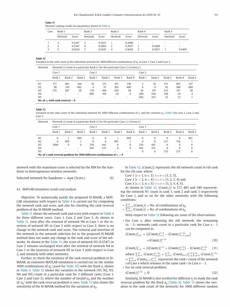
Furthermore, Fig. 6 illustrates the percentage of unreliable ranking
of the classical MADM methods for 10,0 0 0 different combinations of
a ij with respect to the attribute weight method to the different at-
tribute normalization methods. As shown in Fig. 6 , the percentage
of unreliable ranking of the classical MADM methods is more than
97%, whereas, in the proposed SI-MAAR method is zero (not shown
in Fig. 6 ).
Similarly, Fig. 7 illustrates the percentage of unreliable ranking of
the classical MADM methods for 10,0 0 0 different combinations of a ij with respect to the attribute normalization method to the different
attribute weight methods. As shown in Fig. 7 , among the classical
MADM methods, the percentage of unreliable ranking is less in the
MEW method. Moreover, with the proposed SI-MAAR, the percentage
of unreliable ranking is zero in comparison with the classical MADM
methods.
Hence, it is demonstrated that the proposed Simplified and Im-
proved Multiple Attributes Alternate Ranking (SI-MAAR) method is
the simplest and most improved network ranking method for VHD in
heterogeneous wireless networks. SI-MAAR is a simple method with
less complex and unambiguous network ranking steps when com-
pared to the classical MADM methods: TOPSIS, SAW, MEW and GRA.
Moreover, the proposed SI-MAAR method is completely eliminating
unreliability in network rank and the rank reversal problem of the
classical MADM methods. Hence, the worst time complexity of the
proposed SI-MAAR for n networks of m attributes (including both the
benefit and cost attribute) is O ( m ∗n ).
Finally, SI-MAAR method is one of the best replacements for the
existing classical MADM methods, not only applicable to the field
of real heterogeneous wireless networks, but also to the other fields
where classical MADM methods are widely used in real life.
5. Conclusions and future work
In comparison with the classical MADM methods: TOPSIS, SAW,
MEW and GRA, the proposed Simplified and Improved Multiple At-
tributes Alternate Ranking (SI-MAAR) method eliminated the at-
tribute normalization and weight calculation method’s dependency,
resulting in reliable network rank for the seamless handover with-
out the rank reversal problem. The MATLAB simulation carried out in
10 0 0 and 10,0 0 0 different combinations of network attributes, and
10 0 0 different combinations of the expected attributes, justified net-
work attribute sensitivity, 100% network rank reliability with 0% rank
reversal problem of the SI-MAAR method when compared to the clas-
sical MADM methods.
The future work in this direction can be carried out by verifying
I-MAAR method using network simulator and test-bed for the
erformance metrics like number of handovers, handover delay,
oS of the real-time, non-real-time and interactive applications, and
he percentage of user satisfaction in the heterogeneous wireless
etworks.
eferences
[1] J.I.M. Novella , F.J.G. Castano , QoS Requirements for Multimedia Services, Springer,2007, pp. 67–94 .
[2] Y. Chen , T. Farley , N. Ye , QoS requirements of network applications on the internet,
J. Inf. Knowl. Syst. Manag. 4 (2004) 55–76 . [3] Q. Song , A. Jamalipour , A quality of service negotiation-based vertical hando de-
cision scheme in heterogeneous wireless systems, Eur. J. Oper. Res. 191 (2008)1059–1074 .
[4] Q.T.N. Vuong , N. Agoulmine , Y.G. Doudane , A user-centric and context-aware so-lution to interface management and access network selection in heterogeneous
wireless environments, Elsevier Comput. Netw. 52 (2008) 3358–3372 .
[5] S. Lee , K. Sriram , K. Kim , Y.H. Kim , N. Golmie , Vertical Handoff decision algorithmsfor providing optimized performance in heterogeneous wireless networks, IEEE
Trans. Veh. Tech. 58 (2009) 865–881 . [6] A.-E. M. Taha , H.S. Hassanein , H.T. Mouftah , Vertical Handoffs as a radio resource
management tool, Elsevier Comput. Commun. 31 (2008) 950–961 . [7] S.Y. Hui , K.H. Yeung , Challenges in the Migration to 4G Mobile Systems, IEEE Com-
mun. Mag. 41 (2003) 54–59 .
[8] A. Duda , C.J. Sreenan , Challenges for quality of service in next generation mobilenetworks, in: Proceedings of International Conference on Information Technology
and Telecommunications (ITT), October 2003 . [9] F. Siddiqui , S. Zeadally , Mobility management across hybrid wireless networks:
Trends and Challenges, Elsevier Comput. Commun. 29 (2006) 1363–1385 . [10] K. Aretz , M. Haardt , W. Konhauser , W. Mohr , The future of wireless communica-
tions beyond the third generation, Elsevier Comput. Netw. 37 (2001) 83–92 . [11] N. Nasser , A. Hasswa , H. Hassanein , Handoffs in fourth generation heterogeneous
networks, IEEE Commun. Mag. 44 (2006) 96–103 .
[12] H.J. Wangy , R.H. Katz , J. Giesez , Policy-Enabled Handoffs across heterogeneouswireless networks, in: Proceedings of the 2 nd IEEE Workshop on Mobile Comput-
ing Systems and Applications (WMCSA-1999), 1999, pp. 51–60 . [13] Cisco , Global Mobile data Traffic Forecast Update, Technical Report, Cisco Visual
netwokring Index, 2013 . [14] J. Mrquez-Barja , C.T. Calafate , J.-C. Cano , P. Manzoni , An overview of vertical han-
dover techniques: Algorithms, protocols and tools, Elsevier Comput. Commun. 34
(2011) 985–997 . [15] A. Ahmed , L.M. Boulahia , D. Gaiti , Enabling vertical handover decisions in hetero-
geneous wireless networks: a state-of-the-art and a classification, IEEE Commun.Surv. Tutor. 16 (2014) 776–811 .
[16] J. Mcnair , F. Zhu , Vertical Handoffs in fourth generation multinetwork environ-ments, IEEE Wirel. Commun. 11 (2004) 8–15 .
[17] M. Kassar , B. Kervella , G. Pujolle , An overview of vertical handover decision strate-
gies in heterogeneous wireless networks, Elsevier Comput. Commun. 31 (2008)2607–2620 .
[18] K. Piamrat , A. Ksentini , J.-M. Bonnin , C. Viho , Radio resource managementin emerging heterogeneous wireless networks, Elsevier Comput. Commun. 34
(2011) 1066–1076 . [19] M. Zekri , B. Jouaber , D. Zeghlache , A review on mobility management and verti-
cal handover solutions over heterogeneous wireless networks, Elsevier Comput.
Commun. 35 (2012) 2055–2068 . [20] Y.A.S. Xiaohuan Yan , S. Narayanan , A survey of vertical handover decision algo-
rithms in Fourth Generation heterogeneous wireless networks, Elsevier Comput.Netw. 54 (2010) 1848–1863 .
[21] E. Stevens-Navarro , Y. Lin , V.W.S. Wong , An MDP-based vertical handoff deci-sion algorithm for heterogeneous wireless networks, IEEE Trans. Vehic. Tech. 57
(2008) 1243–1254 .
[22] I. Chamodrakas , D. Martakos , A utility-based fuzzy TOPSIS method for energy ef-ficient network selection in heterogeneous wireless networks, Elsevier Appl. Soft
Comput. 11 (2011) 3734–3743 . [23] F. Ning , P. Zhang , A multiple attribute decision making-based access selection
for heterogeneous WCDMA and WLAN networks, in: Proceedings of InternationalConference on Affective Computing and Intelligent Interaction (ICACII-2012), 10,
2012, pp. 15–21 .
[24] R. Trestian , O. Ormond , G.-M. Muntean , Game theory-based network selection:solutions and challenges, IEEE Commun. Surv. Tutor. 14 (2012) 1212–1231 .
[25] A. Antonopoulos , J. Alonso-Zrate , E. Kartsakli , L. Alonso , C. Verikoukis , Cross layeraccess point selection mechanisms for a distributed queuing MAC protocol, J.
Telecommun. Syst. 53 (2013) 329–342 . [26] Y. Song , P.-Y. Kong , Y. Han , Power-optimized vertical handover scheme for hetero-
geneous wireless networks, IEEE Commun. Lett. 18 (2014) 277–280 . [27] D.E. Charilas , A.D. Panagopoulous , Multiaccess radio network enviroments, IEEE
Veh. Tech. Mag. 5 (2010) 40–49 .
[28] L. Wang , G.S. Kuo , Mathematical modeling for network selection in heteroge-neous wireless networks a tutorial, IEEE Commun. Surv. Tutor. 15 (2013) 271–292 .
[29] G.-H. Tzeng , J.-J. Huang , Multiple Attribute Decision Making: Methods and Appli-cations, CRC Press, Taylor & Francis Group, June 2011 .

B.R. Chandavarkar, R.M.R. Guddeti / Computer Communications 83 (2016) 81–97 97
[
[
[
[
[
[
[
[
[
[
[
[
[
30] M. Behzadiana , S.K. Otaghsara , M. Yazdani , J. Ignatius , A state-of the-art survey ofTOPSIS applications, Elsevier Expert Syst. Appl. 39 (2012) 13051–13069 .
[31] S.-J. Yang , W.-C. Tseng , Design novel weighted rating of multiple attributesscheme to enhance handoff efficiency in heterogeneous wireless networks, El-
sevier Comput. Commun. 36 (2013) 1498–1514 . 32] Y. Kuo , T. Yang , G.-W. Huang , The use of grey relational analysis in solving
multiple attribute decision-making problems, Elsevier Comput. Ind. Eng. 55(2008) 80–93 .
[33] E. Stevens-Navarro , V.W.S. Wong , Comparison between Vertical Handoff
Decision Algorithms for Heterogeneous Wireless Networks, in: Proceedings of the63 rd IEEE Conference on Vehicular Technology (VTC-2006), 2, 2006, pp. 947–951 .
34] Y.-M. Wanga , Y. Luoc , On rank reversal in decision analysis, Elsevier Math. Com-put. Modell. 49 (2009) 1221–1229 .
[35] M. Drissi , M. Oumsis , Performance evaluation of multi-criteria vertical handoverfor heterogeneous wireless networks, in: Proceedings of the IEEE Conference on
Intelligent Systems and Computer Vision (ISCV-2015), 2015, pp. 1–5 .
36] E. Stevens-Navarro , J.D. Martinez-Morales , U. Pineda-Rico , Evaluation of verticalhandoff decision algorithms based on MADM methods for heterogeneous wire-
less networks, J. Appl. Res. Tech. 10 (2012) 534–548 . [37] D. Xenakis , N. Passas , L. Merakos , C. Verikoukis , Mobility management for fem-
tocells in lte-advanced: key aspects and survey of handover decision algorithms,IEEE Commun. Surv. Tutor. 1 (2014) 64–91 .
38] L. Wang , D. Binet , TRUST: a trigger-based automatic subjective weighting method
for network selection, in: Proceedings of the Fifth Advanced International Confer-ence on Telecommunications (AICT-2009), 2009, pp. 362–368 .
39] W. Zhang , Handover decision using fuzzy MADM in heterogeneous networks, in:Proceedings of the IEEE Wireless Communications and Networking Conference
(WCNC-04), 2, 2004, pp. 653–658 . 40] D. He , C. Chi , S. Chan , C. Chen , J. Bu , M. Yin , A simple and robust vertical hand-
off algorithm for heterogeneous wireless mobile networks, Springer Wirel. Pers.Commun. 59 (2011) 361–373 .
[41] K. Ahuja , B. Singh , R. Khanna , Network selection algorithm based on link qual-ity parameters for heterogeneous wireless networks, Elsevier Optik 125 (2014)
3657–3662 .
42] Y.-F. Wen , K.-Y. Hung , Energy efficiency heterogeneous wireless access selectionfor multiple types of applications, Elsevier J. Syst. Softw. 101 (2015) 97–109 .
43] E. Khloussy , X. Gelabert , Y. Jiang , Investigation on MDP-based radio access tech-nology selection in heterogeneous wireless networks, Elsevier Comput. Netw. 91
(2015) 57–67 . 44] A. Celen , Comparative analysis of normalization procedures in topsis method:
with an application to turkish deposit banking market, J. Inf. 25 (2014) 185–208 .
45] J. Lin , Divergence measures based on the shannon entropy, IEEE Trans. Inf. Theory37 (1991) 145–151 .
46] T.L. Saaty , How to make decision: the analytic hierarchy process, Eur. J. Oper. Res.48 (1990) 9–26 .
[47] B.R. Chandavarkar , R.M.R. Guddeti , Simplified and Improved analytical hierarchyprocess aid for selecting the candidate networks in an overlay heterogeneous net-
works, Springer Wirel. Pers. Commun. 83 (2015) 2593–2606 .
48] M. D’Agostino , V. Dardanoni , What’s so special about euclidean distance ? J. SocialChoice Welf. 33 (2009) 211–233 .


![Introductionolano/s2001c24/ch09.pdfIntroduction Perlin ! ! "$#%"& ! ' ( *)%+!,!-[EBERT98],[FOLEY96],[PERLIN85], #. "01 !"02 %3% !"&4 / 5 '6/ 7 !"&8](https://img.pdfslide.net/doc/110x75/5f2baee238fa202afe42d09f/introduction-olanos2001c24ch09pdf-introduction-perlin-.jpg)