Embed Size (px)
Citation preview

Simulated annealing
in
FWA-network planning
Master thesis report by
Niels M. Jørgensen, c948718
Supervisor
Professor Jens Clausen, IMM, Technical University of Denmark
Ph.D. Christian Kloch, L.M. Ericsson A/S, Denmark
Lyngby, 31. July 2001

c948718 Niels M. Jørgensen Simulated annealing in FWA-network planning
Abstract
The planning of FWA-networks is a time consuming process. The aim with this paper
is to find a model that can locate base stations in designspace and connect end-user to
the base stations and solve the model within one hour. This paper describes the exact
mathematical model for the base station location problem in FWA-networks and why
it is not possible to solve the problem using this exact method within the given
timeframe. Instead the base station location problem is solved using the Metaheuristic
Simulated Annealing while minimizing the number of not connected end-users.

c948718 Niels M. Jørgensen Simulated annealing in FWA-network planning
Page 1 of 95
Preface
During the time I was writing this master thesis I was pleased with the assistance form
not only my supervisors. I was also supported by the people at both O/ZA group at
L.M. Ericsson Denmark A/S and Operational Research (OR) -group at Informatics,
Mathematics and Modeling (IMM) at the Technical University of Denmark (DTU). I
am very grateful for this support and I would like to thank all the people who have
contributed to my paper and have been very helpful when things have appeared
impossible. At IMM I would like to thank my co-students Michael Løve, Kim Riis
Sørensen, Mette Krogh-Jespersen and the Ph.D.-students Thomas K. Stidsen and
Jesper A. Hansen for their assistance in all aspects of the project. At L.M. Ericsson I
would like to thank Ulrik Heins and Nils Rinaldi for explaining the mysteries of radio
transmission and Mazeyar Firouzi for helping in mastering C-programming.
Especially I would like to thank my two supervisors. For the academic and theoretical
part, Professor Jens Clausen, IMM at DTU and for the commercial and practical part,
Senior Specialist Ph.D. Christian Kloch, O/ZAF at L.M. Ericsson Denmark A/S.
_______________________________
Niels M. Jørgensen, c948718
IMM, DTU
Lyngby, 31. July 2001

c948718 Niels M. Jørgensen Simulated annealing in FWA-network planning
Page 2 of 95

c948718 Niels M. Jørgensen Simulated annealing in FWA-network planning
Page 3 of 95
Table of contents
Preface ____________________________________________________________ 1
Table of contents ____________________________________________________ 3
Abbreviations _______________________________________________________ 7
1 Introduction_______________________________________________________ 8
1.1 Planning tasks________________________________________________________ 91.1.1 Step 1_________________________________________________________________ 10
1.1.2 Step 2_________________________________________________________________ 11
1.2 Thesis statement _____________________________________________________ 11
1.3 Project visions_______________________________________________________ 12
2 Other researchers work_____________________________________________ 13
3 Conceptual model _________________________________________________ 19
3.1 Design space ________________________________________________________ 19
3.2 End-users___________________________________________________________ 19
3.3 Base stations sites ____________________________________________________ 19
3.4 Radio propagation ___________________________________________________ 19
3.5 Interference_________________________________________________________ 20
3.6 Optimization parameters______________________________________________ 203.6.1 Objective functions ______________________________________________________ 21
3.6.2 Constraints_____________________________________________________________ 22
3.6.3 Model variables _________________________________________________________ 22
4 Mathematical model _______________________________________________ 25
4.1 Optimization models _________________________________________________ 254.1.1 Maximizing minimal load _________________________________________________ 26
4.1.2 Maximizing number of connected end-users___________________________________ 26
4.1.3 Minimize the number of base stations________________________________________ 27
4.1.4 Static multi-criterion solution method________________________________________ 27
4.1.5 Minimal cost function method______________________________________________ 30
4.1.6 Objective functions ______________________________________________________ 32

c948718 Niels M. Jørgensen Simulated annealing in FWA-network planning
Page 4 of 95
4.1.7 Constraints_____________________________________________________________ 34
5 Data analysis _____________________________________________________ 38
5.1 Input data __________________________________________________________ 38
5.2 Refining the data ____________________________________________________ 385.2.1 Distance table __________________________________________________________ 38
5.2.2 Legal connection table____________________________________________________ 38
5.2.3 Graph analysis __________________________________________________________ 39
6 Solving the problem________________________________________________ 42
6.1 Relaxed exact model__________________________________________________ 436.1.1 Finding a set of base stations_______________________________________________ 43
6.1.2 Finding the end-user base station connections _________________________________ 44
6.1.3 Setting the output power level______________________________________________ 44
6.2 Artificial constraints__________________________________________________ 466.2.1 Minimum inter base station distance _________________________________________ 46
6.2.2 Demand controlled transmissions power______________________________________ 48
6.2.3 Transmission area overlap_________________________________________________ 49
6.3 Test run of relaxed exact model ________________________________________ 506.3.1 First test run____________________________________________________________ 51
6.3.2 Second test run _________________________________________________________ 52
6.3.3 Third test run ___________________________________________________________ 54
6.3.4 Fourth test run __________________________________________________________ 55
6.4 Relaxed exact model test run discussion _________________________________ 56
6.5 Relaxed exact model test run conclusion _________________________________ 58
7 Metaheuristic method ______________________________________________ 59
7.1 Problem representation _______________________________________________ 617.1.1 Graph models __________________________________________________________ 61
7.2 Start solution________________________________________________________ 64
7.3 Neighborhood _______________________________________________________ 65
7.4 Solution evaluation___________________________________________________ 657.4.1 Circle overlap __________________________________________________________ 65
7.4.2 Load deviation__________________________________________________________ 66
7.4.3 Tapering ______________________________________________________________ 66

c948718 Niels M. Jørgensen Simulated annealing in FWA-network planning
Page 5 of 95
7.4.4 Not connected end-users __________________________________________________ 67
7.5 Cooling scheme ______________________________________________________ 67
7.6 Stop criterion _______________________________________________________ 68
8 First version of heuristic ____________________________________________ 70
8.1 Testing the Metaheuristic _____________________________________________ 71
8.2 Parameter setting ____________________________________________________ 718.2.1 Cooling rate ____________________________________________________________ 73
8.2.2 Global iteration _________________________________________________________ 73
8.2.3 Local iteration __________________________________________________________ 73
8.3 Test run of first version _______________________________________________ 73
9 Second version of heuristic __________________________________________ 76
9.1 New constraints______________________________________________________ 779.1.1 Maximal simple overlap __________________________________________________ 77
9.1.2 Tapering ______________________________________________________________ 77
9.2 Neighborhood _______________________________________________________ 78
9.3 Evaluation __________________________________________________________ 79
9.4 Test run of second version _____________________________________________ 809.4.1 Does the improvements actually make the heuristic able to provide a good solution? ___ 81
9.4.2 What is the best setting of the parameters cooling rate, local iteration and global iteration?
__________________________________________________________________________ 84
9.4.3 What is best: many short optimizations or one long optimization?__________________ 85
9.4.4 Can the heuristic provide a good solution when setting the number of base stations it self?
__________________________________________________________________________ 87
9.4.5 How long time does the heuristic need in order to find the best solution? ____________ 89
9.5 Heuristic method test run discussion ____________________________________ 90
9.6 Heuristic method test run conclusion ____________________________________ 90
10 General discussion _______________________________________________ 91
11 General conclusion _______________________________________________ 92
References_________________________________________________________ 93
Appendices ________________________________________________________ 95

c948718 Niels M. Jørgensen Simulated annealing in FWA-network planning
Page 6 of 95

c948718 Niels M. Jørgensen Simulated annealing in FWA-network planning
Page 7 of 95
Abbreviations
FWA Fixed Wireless Access
PMP Point-to-Multipoint
IP Internet Protocol
ATM Asynchronous Transfer Mode
PSTN Public Switching Telephone Network
BAS Broadband Access System
bps bits pr. Second
GSM ‘Global System of Mobile communications’ or ‘Groupe Spéciale
Mobile’
UMTS Universal Mobile Telecommunication System
LOS Line of Sight
C/I Carrier to interference signal ratio
ISP Internet Service Provider

c948718 Niels M. Jørgensen Simulated annealing in FWA-network planning
Page 8 of 95
1 Introduction
A typical connection from the end-users to a plain old telephone system or an Internet
service provider (ISP) is via fixed lines. Another option is to use Fixed Wireless
Access (FWA) which provides a fast establishment and/or expansion of the
connection between operator and end-user. This report considers the planning of
networks starting at a level where location and demand of each end-user and location
of potential base station sites within the service area are known. Today, the radio
network planning is done manually. Depending of the size of the desired network the
process takes between 3 to 5 days for one person. This gives rise to promote use of
computers utilizing operational research to speed-up this process.
The aim for this project is to create mathematical models for tasks of the planning
process, identifying the necessary input data and defining planning parameters that
identify the quality of the network. Another important part is deciding the criteria that
make it possible to detect success when planning.
The FWA system applied in this master thesis is the Ericsson MINI-LINK Broadband
Access System (MINI-LINK BAS). The MINI-LINK BAS system provides
connection between IP/PSTN/ATM backbone network and the end-user service
terminals. The backbone network is connected to the base stations and one base
station can be connected to a number of end-users (Point to Multipoint access (PMP)).
One base station can host up to 6 sectors and each sector has a capacity of 37 Mbps
Gross bit rate full duplex. One sector covers the end-users in an area within an angle
of 90° with a maximum transmission range at approximately 5 km. This means that a
base station with 4 sectors have a total potential coverage area that can be
approximated by a circle with center at the base station and a radius of maximum 5
km.

c948718 Niels M. Jørgensen Simulated annealing in FWA-network planning
Page 9 of 95
1.1 Planning tasks
One of the major tasks is identifying the best location of base stations. The primary
cost of the network is the cost of establishing base stations. Hence, the object is to
minimize the number of base stations while maintaining ‘sufficient coverage’.
‘Sufficient coverage’ is a matter of definition similar to the success parameter. The
operator decides whether the network requested has to cover all potential end-users,
or that the success parameter of e.g. 80% capacity utilization for base stations is
acceptable. There exists other ways of defining the best network for the actual
operator but these two are the most common. In the typical real-life planning process
the first question in the inquiry is the cost of covering all end-users with sufficient
capacity. Second question is how many end-users are covered with a lower number of
base stations, and is this number of end-users above operator’s minimum service
limit. This means that it is desirable to design the planning model in a way where both
planning with unlimited and fixed numbers of base stations are possible.
Current computerbased tools for assisting in the planning process are only capable of
computing the coverage once the base stations have been placed, and not placing the
base stations themselves.
This gives the primary task of this project; find a model that can place base stations
and connect end-users to base stations. Firstly it is necessary to define limitations and
assumptions in the model in order to make the problem manageable.
When dealing with radio signals it is important to take radio propagation loss between
transmitter and receiver into account. Unfortunately it is very complicated to compute
this value due to its dependency of the topography of the surface in the coverage area
e.g. vegetation, buildings etc. Hence, in this model it is decided to reduce the planning
area from a 3-dimensional into a 2-dimensional plan. Connections between base
stations and end-users are pre-computed in the 3-dimensional plan in order to identify
where line of sight (LOS) between transmitting and receiving antennas exists. Finally,
in the 2-dimensional model the propagation loss is assumed linear dependent of
transmission distance and transmission power, measured on a logarithmic scale.

c948718 Niels M. Jørgensen Simulated annealing in FWA-network planning
Page 10 of 95
End-users are located in the planning area and identified by the coordinates and their
demand measured in bps. Potential sites for base stations are also given in the plan,
identified by their coordinates.
Connecting end-users to base stations is done by connecting the end-users to the
nearest base station. This is done while monitoring whether the sum of end-user
demand is less than or equal to, the maximal capacity of the base station and that the
distance between the base station and the end-user is less than 5 km. To do this it is
necessary to simplify the model of the base station in a way where the coverage area
of each base station is assumed to be one circular area instead of four sectors of 90
degrees. The maximal capacity of the base station is simply computed as the product
of the number of sectors and the maximal capacity of each sector. The distance to the
most distant end-user from each base station defines the radius of the coverage circle
of the base station. It is desirable that the overlap between any pair of coverage circles
is minimal due to interference.
The actual planning of the network can be divided into two separate steps as follows:
1.1.1 Step 1
Create a network with total coverage and sufficient capacity for all end-users in the
area while maximizing the minimal load on each base station and minimizing the
overlap between coverage circles.
The output of this step is a plan that gives the number of base stations, the location of
each base station and all base station-end-user connections. This information gives the
operator an opportunity to decide if the number of base stations is acceptable or that
another optimization with a fixed number of base stations has to be made. An
optimization with a fixed number of base stations is as follows:
c948718 Niels M. Jørgensen Simulated annealing in FWA-network planning
Page 11 of 95
1.1.2 Step 2
Find maximal coverage with a fixed number of base stations while maximizing the
minimal load on each base station, and minimizing the overlap between circles.
When step 2 has been performed it should be checked whether the number of end-
users connected is above the minimum service limit.
The planning is performed, aiming at covering the expected demand after a period of
e.g. 8 years. Identifying milestones for the rollout plan is done by ranking the base
stations by the load on each base station. Base stations are then established
successively starting with the one having the most load. This means that milestones
for year 3 and 5 are given by the pace of the rollout progress and not by a separate
optimization aiming at year 3 and 5.
1.2 Thesis statement
Summing up, the formulation of the aim of this project is:
Develop and implement a mathematical model that can locate base stations, connect
end-users to base stations and find a way to solve the model spending less time than
solving the location problem manually.

c948718 Niels M. Jørgensen Simulated annealing in FWA-network planning
Page 12 of 95
1.3 Project visions
The overall perspective with this project is to do the first step in the development of a
planning tool that can assist in the planning of any wireless communication network
such as GSM, UMTS, FWA and others. The idea is to create a core program that, with
the correct input files is able to assist in the planning process. (See below)
Input files
Core program
End-user
Current network
(if exist)
Covering area
Location of potential
base station sites
Equipment data
Frequency
Output file.Base station locations
Frequency plan
End-user – base station connection

c948718 Niels M. Jørgensen Simulated annealing in FWA-network planning
Page 13 of 95
2 Other researchers work
So far it has not been possible to find articles describing the base station location
problem especially for FWA networks. The search has been performed at The
Technical Knowledge Center & Library of Denmark (DTV). The searches were
performed using keywords like ‘Fixed Wireless Access’, ‘Broadband’, ‘Coverage’,
‘Location’ and ‘Radio network’. Instead a number of articles about general base
station location and about base station location for cellular networks such as GSM
900 and UMTS emerged. The question is if the experience in these articles is
applicable in FWA networks.
The aspects considered in the articles spans from modeling the movements of the
mobiles in design space to describe different solution methods of base station location
models. Additionally the design space can be represented as either continuous or
discretized in 2- or 3-dimensional space.
All results and illustrations in this section is from the respective articles.
Shih-Tsung Yang and Anthony Epremides have in the article [1] worked with the
problems related to select location and transmission power of base stations while
maximizing the minimum throughput among the mobiles. The major issue of the
article is to model the movements of the mobile terminals and argue that this
simulation is correct. The design space is discretized into a grid of legal points. The
movement of the mobile terminals is simulated by a random walk between points.
Over time the movements of the mobile terminals converge towards a steady state.
The traffic to each terminal is assumed to be a Bernoulli packet arrival process with a
given rate. The maximal coverage area with respect to load is the area where the
transmission capacities of the base stations can match the demand of all terminals in
the coverage area. In areas where there is low traffic the limiting factor is the
attenuation of signal power from the base station. The modeling of the signal loss is
like the questions about solving the model only briefly touched.

c948718 Niels M. Jørgensen Simulated annealing in FWA-network planning
Page 14 of 95
The article [2] by Calégari P et al. focus on problems related to base station location
in UMTS networks. The article uses a graph theoretical representation of the problem
structure. The design space is tiled using a grid. A node represents each tile in the grid
and an edge connects the node with each of the base stations that can cover the node.
See Figure 1. This gives a bipartite graph with tile nodes on one side and base station
nodes on the other. The solution method suggested in the articles is the graph
theoretical problem ‘Minimum dominating set’. This means find the minimum set of
base stations that covers all end-users. This problem has been proved to be NP-hard.
The primary aim of the article is to describe a solution method based on a genetic
algorithm. The results from a test run on a 70 km x 70 km planning area did not
produce satisfactory solutions but the algorithms are still under development. One
area of special interest is to reduce the size of bipartite graph.
Figure 1
The graph theoretical approach in article [3] by Charmaret B. et al. is different. Here
the propagation model added to each potential base station site is based on one type of
antenna. A graph is created where a node represents each potential base station site. If
two sites have a coverage area in common that is over a given threshold, an edge is
added between the respective nodes see Figure 2. In this graph the solution is given
by the graph theoretical problem ‘Maximum independent set’. This means find a
maximum set of base stations that are not connected. The problem is solved using 7
different stepwise heuristic methods and the results are analyzed to find the method

c948718 Niels M. Jørgensen Simulated annealing in FWA-network planning
Page 15 of 95
that gives the best coverage. The article pays most attention to select the best overlap
threshold value. According to the article the success parameter when evaluating a
given overlap threshold value is either the number of selected base stations or the
relative coverage.
Figure 2
For indoor applications using micro cells the location problems is in many ways
similar to the base station location problem. In [4] Ivan Howitt and Seung-Yong Ham
proposes a solution method for the indoor location problem. This is a heuristic way
using a Wiener process to model the objective function. The Wiener process is a
model where optimality is defined using a stochastic model and then the stochastic
model is optimized.
The overall idea of the method is the following: The process is based on evaluating a
number of solutions found by guessing. Due to the fact that the Wiener process is a
stochastical process it is assumed that the process in some way ensures that the
guesses are evenly distributed in design space. When the solutions are evaluated local
search is performed from the best of the global search solutions. Furthermore, the
article is dealing with indoor applications utilizing two base stations. In the FWA-
network the number of base stations is typically in the size 10-20.
In article [5] by Margaret H. Wright, no model is proposed but it applies the base
station location problem as an example of complex problems where exact methods are
rarely usable. To solve these problems a direct search method is suggested. This
solution method is suitable if the objective value is a scalar as a function of a number

c948718 Niels M. Jørgensen Simulated annealing in FWA-network planning
Page 16 of 95
of parameters. The method is called Nelder–Mead ‘simplex’1 method. This method is
a non-exact method able to solve problems in continuos solution space though it is not
possible to determine how close the given solution is to the optimal solution.
Both [4] and [5] do only pay attention to solve large location problems. The actual
modeling of the problem is either limited or non-existing. The primary reason why the
authors focus on base station location problem is to show how these solving methods
handle hard optimization problems. No numeric results are shown in any of the
articles.
Hanif D. Sherali et al. describes in [6] a model that locates n base stations in an indoor
environment. The design space is discretized into a grid where each tile represents an
end-user. The location of base stations is found by a search in continuous solution
space. The final locations of the base stations are where a convex combination of two
values is minimal. The first value is the minimum average of all path losses between
base station and end-user. Second value is minimum maximal path loss between base
stations and end-users. The article proposes three methods to solve the problem. All
methods are heuristic search algorithms and hence require an initial solution. The
initial solution is found by minimizing the sum of weighted squared Euclidean
distances between base stations and end-users. The methods to improve the solution
are Hooke and Jeeves’ method, Quasi Newton method and Conjugated Gradient
search. In order to reduce the computational work the problem is solved as a number
of problems. Initially the problem is solved where the grid density is sparse, later the
grid is increased. Thereby the number of points to be evaluated in the beginning is
reduced, later the solution is refining by increasing the grid density. The results of test
runs using the threes methods placing 2 base stations show a final solution within 8%
of an optimal solution. Best is Conjugated gradient search where all test runs are
within 4% from an optimal solution.
1 The Nelder-Mead “simplex” have no relation to the simplex methods of linear optimization

c948718 Niels M. Jørgensen Simulated annealing in FWA-network planning
Page 17 of 95
In the article [7] Dimitris Stamatelos and Anthony Ephremides describe their work
with placing base station in an indoor environment. The design space is discretizied
into a grid. Mobiles can only be placed at points in the grid, whereas the location
problem of base stations is solved in both continuous and discrete space and both
omnidirectional and adaptive antennas at base stations are investigated. The location
problem is modeled in a way where the design space is divided into 4 types of area.
Cell area, Covered area, Interfered area and Uncovered area. Cell area is the
collection of grid points where the signal strength from at least one base station is
greater than a given receiver threshold. Covered area is a collection of points in the
Cell area where the carrier to interference relation is greater than a given threshold.
Interference area is Cell area minus Covered area and Uncovered area is the rest of
the design space. The objective of the model is to minimize a convex combination of
Uncovered and Interference area by finding the location of each base station and the
transmission power. The methods proposed for solving the model in continuous space
are Steepest descent and Downhill simplex. The Steepest descent method makes use
of the gradient of the objective function to find the next step of the algorithm. The
downhill simplex is similar to the Nelder-Mead simplex method mentioned in [5]. In
the discrete space where most work in this article has been done, the model is solved
using the Hopfield and Tank neural network. In test runs placing 3 base station with
omnidirectional antennas the steepest descent method gave worst results. Best results
were achieved with the Hopfield and Tank neural network. Of the 200 simulations
with neural network only 3% did not converge. All results were within 4% from
optimal solution. In the test run with adaptive antennas at the base stations the Nelder-
Mead simplex method produced a solution 50 % from optimal solution. The steepest
descent algorithm failed to converge but the neural network produced solutions
between 17 and 28 % from optimum.
Summing up the result of the article search. At best the articles can be used as a
collection of ideas when designing models for FWA. In general the articles only focus
on a small part of the entire process of creating the models for layout and propagation
and solve the layout problem whereas the rest of the process is only sparsely
described.

c948718 Niels M. Jørgensen Simulated annealing in FWA-network planning
Page 18 of 95
The steady state of the moving mobiles in article [1] illustrates the theoretical
similarities between mobile systems and FWA systems.
In article [2] the similarity between FWA and cellular networks where tiles are
replaced by end-users is obvious using this representation. As in the FWA case the
objective in the UMTS case is to find a set of base stations that cover a maximum
number of tiles/end-users using a minimum number of base stations.
In article [3] the method described appear to be directly applicable in FWA despite
the article describe UMTS planning.
The articles [4] and [5] describe methods for optimization of all kinds of large integer
problems which means methods that also must be usable to solve FWA problems.
Article [6] and [7] deal with problems related to indoor application. These problems
usually only need a lower number of base stations compared to FWA. This gives the
opportunity to perform exhaustive search in order to find optimal solution for
comparison with the heuristic solution.

c948718 Niels M. Jørgensen Simulated annealing in FWA-network planning
Page 19 of 95
3 Conceptual model
3.1 Design space
Design space for a FWA network is the geographical area that is sought covered. In
the model this area is represented as a 2-D coordinate system.
3.2 End-users
End-users are the final consumers in the network. Their demands are voice, video and
data services. The traffic load for these services is dynamic and it is represented by
the average traffic load and the peak traffic, both in bits/sec. The load is the expected
load of the end-user at a given year. The location of the end-user is either a company
or a private domicile. In the model, each end-user address is converted into a
coordinate set in the 2-D model design space. End-users are identified by the index i
in the model. The demand of each end-user is given by his/her average load and is the
one used in this planning.
3.3 Base stations sites
Potential base station sites are locations where it is possible to place a base station.
These sites are indexed by j and k and represented by a geographical coordinate set. In
the model these values are converted to a set of coordinates in the 2-D model design
space. The capacity of each base station is measured in bits/sec. Like in the case of
end-users the capacity is converted into a single number.
3.4 Radio propagation
The attenuation of radio signals is the limiting factor when considering the possible
distance between base station and end-user. The attenuation is dependent of factors
like obstructing buildings, rain attenuation, etc. For FWA the requirement for
connection between base station and end-user is line of sight, LOS. Simplified, ‘LOS’
means it is possible for the base station antenna and the end-user antenna to ‘see’ each

c948718 Niels M. Jørgensen Simulated annealing in FWA-network planning
Page 20 of 95
other. In the model the radio attenuation measured in dB is assumed linear dependent
of the Euclidean distance between base station and end-user. A potential connection
between a base station and an end-user requires that the Euclidean distance is below
maximum transmission distance due to signal attenuation and where LOS exists. The
signal strength at the end-user is assumed to be the transmitted power minus an
attenuation constant multiplied by the Euclidean distance between end-user and base
station.
3.5 Interference
When the network consists of more than one base station using the same frequency or
one of the two adjacent frequencies, there is interference. Interference is measured as
the relationship between the Carrier signal from the assigned base station and the sum
of Interfering signals from other base stations, C/I. The interference is only interesting
at the points where end-users are located. In this model the C/I is computed as the
ratio of the signal strength at each end-user from its assigned base station and by the
sum of signal strengths at the end-user, from all the rest of the base stations. The
signal strength at an end-user from a given base station is computed according to the
model mentioned in the preceding section ‘Radio propagation’ likewise is the
interfering signal strength computed.
3.6 Optimization parameters
In step one in the network design process, the aim for the radio planner is to create a
base station layout that ensures that all end-users are connected to a base station. This
can be done numerous ways. Operators can have different quality targets toward the
layout of the network such as “a maximal number of end-users must be covered” or
“the load on each base station must be maximal”. Most of these targets can be
expressed using the three parameters: active base stations, end-users and load on base
stations.

c948718 Niels M. Jørgensen Simulated annealing in FWA-network planning
Page 21 of 95
The most expensive components in an FWA-network are the base stations including
the cost of the sites. This makes it attractive to minimize the number of base stations
in order to reduce the costs of the network.
The load on each base station expresses the future options to develop the network,
besides the potential revenue on the individual base station. The decision of placing a
base station at a given location, or not, is made on the basis of the expected load at the
location. Due to the initial cost of establishing base stations it is not attractive to
establish a base station if the expected load at the location is less than a given
threshold. In order to prepare the network for future expansion in the number of end-
users using the established network, is it desirable to have a close to even load on all
base stations.
Finally the total number of end-users connected to base stations is an important
parameter. The number of connected end-users is obviously closely related to the load
on the base stations.
This gives three options for objective functions where the selected parameter is
optimized. Instead of utilizing only one of the objective functions it is possible to use
all three in a three-criterion solution method. Another option is to add a ‘cost’ on each
parameter and then optimize the total ‘cost’ of the network. A special case of this
function is where the sum of ‘cost’ constants is 1. This special case is called a convex
combination.
Regardless of the objective function chosen the function is optimized with respect to a
lot of constraints. These constraints are imposed by the system limitations and
expressed mathematically.
3.6.1 Objective functions
- Maximizes the minimal load variable.
- Minimizes the number of base stations (in step one only)
- Maximizes the number of end-users connected (in step two only)

c948718 Niels M. Jørgensen Simulated annealing in FWA-network planning
Page 22 of 95
- Optimize a convex combination of two or three of the parameters, number of
active base stations, number of connected end-users and maximal minimal load on
a base station.
- Minimize the total ‘cost’ of the network.
3.6.2 Constraints
- The sum of capacity demands connected to one base station must be larger than or
equal to the minimum load variable or a minimum load constant.
- The sum of capacity demands connected to one base station must be less than or
equal the maximum base station capacity.
- Each end-user must be connected to only one base station.
- End-users can only be connected to active base stations.
- End-users can only be connected to base stations if it is possible to get line of
sight.
- The C/I at each end-user must be larger than or equal to a given threshold value.
- The signal strength at each end-user from the assigned base station must be larger
than or equal to a given threshold value.
3.6.3 Model variables
When modeling these objective functions and constraints a number of factors are
identifying base stations, capacity, legal connections, etc. The definitions of these
factors are as follows [9]:
Decision factors:
The optimization algorithm can adjust these variables within the given range, in order
to achieve the best solution.
Conditional factors:
These values vary when decision variable values are altered, identifying the
conditions of the system.

c948718 Niels M. Jørgensen Simulated annealing in FWA-network planning
Page 23 of 95
Structural factors:
These values are assumed constant within the time interval considered. Hence, the
model cannot change these values.
Environmental factors:
Factors that are controlled outside the system considered but can affect the conditions
of the system. These factors do not appear in this paper.

c948718 Niels M. Jørgensen Simulated annealing in FWA-network planning
Page 24 of 95
The variables in the model are as follows:
Factor Symbol Role Range
End-user id i -- {1,2,..,(I-1),I}
End-user coordinate xi,yi Structural factor [0;Xmax, 0;Ymax]
End-user demand di Structural factor [0;CAPlim]
Base station site id j,k -- {1,2,..,(J-1),J]
Base station coordinate xj,yj Structural factor [0;Xmax, 0;Ymax]
Transmission power at base station Pj Decision factor [0;Pmax]
Base station at site bj Decision factor {0,1}
Base station capacity CAPlim Structural factor R+
Legal connections kij Structural factor {0,1}
End-user – base station connec. cij Decision factor {0,1}
Minimum number of end-user basestation connection
Cmin Decision factor {0,1..(I-1),I}
Signal at end-user from basestation
sij Conditional factor [0;pj]
Minimum C/I C/Ilim Structural factor R
Minimum signal strength SIGlim Structural factor R
Load on base station L Conditional factor [0;CAP]
Min. load on each base station Llim Decision factor [0;CAP]
Distance between end-user andbase station
Distij Structural factor R+
Signal attenuation constant Att. Structural factor R
Distance between twoBase stations j,k
Oj,k Structural factor R+
Minimum distance between twobase stations
Omin Structural factor R+
Objective value Z Conditional factor R
Various costs Q -- R
‘Big model constant’ M -- →∞
Distance between base station jand most distant end-user
connected to jrj Conditional factor [0;Max_dist]
Density weight factor wi Structural factor R+

c948718 Niels M. Jørgensen Simulated annealing in FWA-network planning
Page 25 of 95
4 Mathematical model
4.1 Optimization models
When designing mathematical models the aim is to create the equations that identify
the constraints of the system and the objective function that expresses the value of the
system. When these equations have been formulated the model can give the answer
whether a given parameter (decision factor) setting is legal or not and identify the
value of the system as a single number. The model can now be used to find the
parameter setting that gives the best system value by optimizing the objective
function.
As mentioned, three parameters identify the value of the network design. These
parameters are ‘minimal load on base stations in the solution’ named L, ‘number of
connected end-users’ found as the sum of ci,j-variables and ‘number of active base
stations’ found as the sum of bj-variables.
Despite it is only possible to optimize one parameter at a time none of the parameters
can be isolated and optimized without considering the two other parameters. When
one parameter acts as the objective function at least one of the other parameters has to
be inserted into the model with an upper and lower bound. When setting the
parameter bounds in the model, care must be taken not to make the model infeasible.
This is regardless of the number of parameters inserted in the model is one or two.
E.g. consider a situation where the minimal load on base stations is sought
maximized. The number of base stations is bounded to a value where the product of
base stations capacity and number of base stations is less than the total sum of end-
user demands. In this situation the model is infeasible if all end-users must be covered
according to the constraint on the number of end-users. However, removing the
constraint on the number of base stations will not guarantee that the model is feasible.
Depending on the distribution of the end-users the model could still be infeasible due
to the constraints regarding interference. When using a multi-criterion solution
method the valid combinations and ranges of these bounds are identified as a part of
the process.

c948718 Niels M. Jørgensen Simulated annealing in FWA-network planning
Page 26 of 95
4.1.1 Maximizing minimal load
In step one of the optimization process the aim is to cover all end-users and to have a
maximal minimal load L on each base station. This outlines a model with an object
function that maximizes the minimal load and a constraint that set the sum of end-
users equal to the total number of end-users. The sum of the number of base stations
can be left unconstrained.
One obvious element in getting a maximal minimal load L on the base stations is to
distribute the total load over a minimal number of base stations bj. The minimal
number of base stations that can cover all end-users is found by dividing the total sum
of end-user capacity demands with the base station capacity. This number is then
rounded up to the nearest integer. One upper limit of L is found as the total sum of
end-user capacity demands divided by the minimum number of base stations needed.
Intuitively, this objective function should provide a solution with a minimum number
of base stations but it is not necessarily the case. The reason is that end-users are not
evenly distributed in design space and base stations can only be located at discrete
locations.
4.1.2 Maximizing number of connected end-users
In step two of the design process the idea is to choose a fixed number B of base
stations and then find the maximal number of end-users that can be connected to B
base stations among the available. The obvious objective function for this
optimization is a model that maximizes the number of connected end-users. This
model needs a bound on the number of active base stations.
A constraint that sets a minimum for the load on each base station can be added to the
model. However, here it is important to notice that if the minimal load is set too high
the model is infeasible. Omitting the load constraint, the model is always feasible.
Though, the load on some of the base stations could end with zero.

c948718 Niels M. Jørgensen Simulated annealing in FWA-network planning
Page 27 of 95
4.1.3 Minimize the number of base stations
A model that minimizes the total number of base stations while keeping the number of
connected end-users above the lower bound, will at the same time implicitly
maximize the average load on the base stations. A minimal number of active base
stations require as many end-users as possible at each active base station. Whereas
getting a result with maximal minimal load is unlikely the case. Again this is due to
end-users not being evenly distributed in design space and it is only possible to locate
base stations at discrete locations.
This objective function is not directly necessary in none of the two planning steps but
is usable if the operator requires a coverage of e.g. 90% of the end-users and wants to
know how many base stations are needed.
Summing up on these three relations, they indicate that a good final solution is a
tradeoff between these three parameters. Methods considered for finding a good or
best solution in this paper are the cost function and the multi-criterion solution
method.
4.1.4 Static multi-criterion solution method
A multi-criterion method is a series of optimization. In each optimization one
parameter is selected to be in the objective function. Some or all of the remaining
parameters are inserted in the model, each one limited by two equations that sets the
upper and lower bound for the parameter. This means finding the best solution for
parameter A while maintaining given values for parameter B, C, etc. Figure 3
illustrates the result of an imaginary 2-parameter example. The objective function
optimizes parameter B and a constraint bounds parameter A to be greater than or equal
to a given value in each optimization process. The figure shows the optimized value
of parameter B at each fixed value of parameter A.

c948718 Niels M. Jørgensen Simulated annealing in FWA-network planning
Page 28 of 95
2-criterion solution method
0
0.5
1
1.5
2
2.5
3
3.5
4
4.5
0 0.5 1 1.5 2 2.5 3 3.5Parameter A
Para
met
er B
Figure 3
As can be seen from Figure 3 no solution exists for values of A greater than 3.
Equally, for values greater than 4 for parameter B the problem is infeasible.
In the actual network Figure 3 could illustrate the result of a series of optimizations
where one of the parameters is uncontrolled. Consider a situation where the aim is to
maximize the minimal load while maintaining a fixed number of end-users connected.
In this case let parameter B illustrate maximal minimal load and parameter A be the
number of end-users connected. At each optimization the number of end-users is fixed
at a value within the desired range and after each optimization the result is plotted as a
coordinate set of (end-users connected, maximal minimal load). Due to the fact that
end-users are not uniformly distributed in design space, it is very likely that the
maximal minimal load is low if the number of end-users connected is high and vice
versa. Note that in this situation it is not necessary to control the number of base
stations though it is possible.
For the actual problems with 3 parameters the process is technically the same but
naturally becomes more time consuming due to the increased number of combinations
of parameter settings.
The total model for finding the maximal minimal load in step one in the optimization
process is shown in Model 1. Notice that L in this model is a variable.

c948718 Niels M. Jørgensen Simulated annealing in FWA-network planning
Page 29 of 95
( ){ } [ ] [ ]limmax
ijijjijj
limj
ijij
jijijlimij
jijij
jijij
jij
jlimi
iij
ijiij
CAPLsPpcb11 Eq.JjI,ijisAttdistpkb
10 Eq.JjI,iiSIGsc
9 Eq.JjI,iicsICkc1s
8 Eq.JjI,ijibkc
7 Eq.JjI,ii1c
6 Eq.JjI,ijbCAPdc
5 Eq.JjI,ijLMb1dcwrt.
LaxMZ
;0;;;0;1,0,,
)(/)(
,
)(
)(
∈ℜ∈∈∈
∈∈∀=⋅−⋅⋅
∈∈∀≥⋅
∈∈∀⋅≤⋅�
���
�⋅−⋅
∈∈∀⋅≤
∈∈∀=
∈∈∀⋅≤⋅
∈∈∀≥⋅−+⋅
=
Model 1
Due to multiplication of two or more variables in Equation 9, 10 and 11 this model is
non-linear and hereby not necessarily optimally solvable.
Step two in the optimization process is to find the maximal number of end-users
connected to a given number of base stations. A model similar to Model 1 with a few
adjustments is used for this purpose. The objective function in this case is maximizing
the number of end-users connected. Equation 7 is changed from equality to an
inequality. Finally, a constraint is added that ensures that the sum of bj-variables is
equal to the desired number of base stations. Additionally, a constraint that controls
the minimum load L on base stations is added. Unfortunately it is not possible prior to
the optimization to give a value combination for number of base stations and
minimum load L that necessarily makes the model feasible.
Rethinking the modeling of step two could as well be a model similar to Model 1
where Equation 7 is changed from equality to an inequality and another constraint is
added. This constraint set a lower bound to the sum of connected end-users Clim but
leaves the number of base stations unconstrained. As mentioned earlier, this model

c948718 Niels M. Jørgensen Simulated annealing in FWA-network planning
Page 30 of 95
will implicitly reduce the number of base stations, though not necessarily leading to a
global minimum. The operator has to set a range for the desired coverage instead of
setting a fixed number of base stations. Using the static multi-criterion solution
method, one optimization is made for each value of the Clim-value within the given
range set by the operator. For each setting of the Clim the optimization will provide an
optimized value for L and the number of base stations. When optimizations with a
sufficient number of Clim-values within the given range have been performed, the
operator’s tradeoff can be performed on the basis of the network options.
4.1.5 Minimal cost function method
The basic idea of the cost function method is to use costs to guide the model towards
a solution with the desired qualities. When using the minimal cost function the most
difficult task is to put a cost on each parameter. E.g. the cost of a base station can be
set relatively easily by using the cost of the base station in money. It gets more
complicated when it comes to the cost of the parameter end-user and load.
One option to put a cost on the parameter end-user is to use the loss of income from
each not connected end-user. Then the optimization model will weight the cost of
adding an extra base station and get the extra income when extra end-users get
connected.
Adding costs to load can be done in two ways. One option is to add a cost on load
deviation from a given desired load on each base station. The problem here is that the
difference between the desired load and the actual load can be either positive or
negative. Using ‘absolute value’ or ‘difference squared’ functions to avoid this
problem makes the objective function non-linear. The effect of this cost is that it finds
the minimal sum of deviations from the given load level. Another option is to add a
cost to the non-utilized capacity at each base station. This method is relatively easy to
implement by multiply the cost value and the difference between capacity and load on
each active base station. The cost value in connection with non-utilized demand can
be set as the lack of income of each non-utilized kbps.

c948718 Niels M. Jørgensen Simulated annealing in FWA-network planning
Page 31 of 95
The major disadvantage with such a formulation of the objective function is that it can
be difficult to find the correct weight of the cost values in order to get the desired
effect on the network design. Thus, summing disadvantage costs gives a total
disadvantage and no information about disadvantage deviation. This hides undesired
variations in e.g. load on different base stations. Hence, this objective function
maximizes the average load with no respect to deviation, whereas maximizing the
minimal load objective function both maximizes the minimal load and minimizes the
deviation between load on base station.
The mathematical formulation of the minimum cost model is as follows:
( ){ } [ ]CAPlcb
11 Eq.JjI,ijisAttdistpkb
10 Eq.JjI,iiSIGsc
9 Eq.JjI,iicsICkc1s
8 Eq.JjI,ijibkc
7 Eq.JjI,ii1c
6 Eq.JjI,ijbCAPdcwrt.
QcQbQdcbCAPmin
ijijjijj
limj
ijij
jijijlimij
jijij
jijij
jij
jlimi
iij
EUij
ijj
BSjj
Li
iijjlim
;0;1,0,
,
)(/)(
,
∈∈
∈∈∀=⋅−⋅⋅
∈∈∀≥⋅
∈∈∀⋅≤⋅�
���
�⋅−⋅
∈∈∀⋅≤
∈∈∀=
∈∈∀⋅≤⋅
���
���
�⋅+⋅+⋅���
�
� ⋅−⋅
Model 2
As can be seen, most of this model is equal to the maximizing minimal load model
apart from a minimum load limit, Equation 5, and the object function, Equation 4.
Similarly, the model is non-linear due to Equation 9, 10 and 11. In this formulation
the model will find a solution that covers all end-users at the minimal cost with
respect to the given costs Q.

c948718 Niels M. Jørgensen Simulated annealing in FWA-network planning
Page 32 of 95
4.1.6 Objective functions
The exact mathematical formulations of the object functions mentioned in the
previous section are as follows:
)(LMaxZ =
Equation 1
This function maximizes the minimum load variable L. Hence, at least one constraint
has to be added to the model that bounds either minimum number of end-users
connected or minimum number of active base stations.
JjbMinZj
j ∈=
Equation 2
This function minimizes the number of active base stations. When using this function
with a constraint for minimum number of end-users connected, the average load on
base stations is maximized. The difference from using Equation 1 is that in Equation
1 the minimum load is maximized whereas with this equation and the minimum
number of end-users-constraint, the minimum load is uncontrolled.
Modifying this objective function to maximize the sum of base station variables and
use it in connection with a minimum load constraint it finds the maximal set of
profitable base stations.
JjIijicMaxZi j
ij ∈∈∀= ,,
Equation 3
This function maximizes the number of end-users connected. Like Equation 1 and
Equation 2 this objective function needs at least one constraint to control either the
load on each base station or the number of base stations.

c948718 Niels M. Jørgensen Simulated annealing in FWA-network planning
Page 33 of 95
BEqJjIiQcQbQdcbCAPMinZ
AEqJjIiQcQbbQdcCAPMinZ
jiijij
jBSjL
j iiijjlim
j j jiijijBSjjL
iiijlim
.4.,.
.4.,.
,
,
∈∈�
���
�⋅+⋅+⋅���
�
� −⋅=
∈∈���
��
�
�⋅+⋅+��
����
�⋅⋅���
�
� −=
Equation 4
These functions minimize the total cost of the network system.
In Equation 4A, the first component, the demand connected to a base station j is
subtracted from the capacity CAPlim. This non-utilized capacity is multiplied a cost
constant QL and the binary variable bj that indicates whether a base station capacity is
available or not. Finally summed over base stations j. Unfortunately, this construction
results in a multiplication of the variables cij and bj which makes the object function
non-linear. It is crucial to have the binary bj variable present otherwise will non-active
base stations contribute in a negative way with the total capacity.
Another way of adding a cost to non-utilized capacity is displayed in
Equation 4B. Here the total demand connected to the base station j is subtracted from
the capacity constant multiplied by the base station variable bj. This formulation is
possible due to a constraint that makes sure that demand only can be connected to
active base stations. This gives, if the bj is ‘0’ then the total demand is also ‘0’.
The rest of Equation 4A and Equation 4B are identical.
In the second component establishing a base station, bj = 1, is multiplied by a cost and
summed over all base stations.
In the last component, the binary variable ci,j, indicating if end-user i is connected to
base station j, is multiplied with the negative cost of not connecting end-user i,
summed over all combinations of i and base station j.
c948718 Niels M. Jørgensen Simulated annealing in FWA-network planning
Page 34 of 95
The advantage with this formulation is the flexibility of the object function. Any
variable in the model can be priced and be added as a component in the object
function. The layout of the function in Equation 4 is only one suggestion on how to
price less desired elements in the network.
4.1.7 Constraints
The system constraints imposed by the system like maximal transmission range, total
bit rate capacity, etc. must be respected. These constraints formulated mathematically
are the following.
( ) JjIijLMb1dci
jiij ∈∈∀≥⋅−+⋅ ,
Equation 5
The connections between end-user i and base station site j multiplied with the demand
at end-user i summed over end-users i, must be greater than or equal to the minimum
load variable L. If base station j is inactive, bj = 0, the second component add a large
constant, M, to the zero-demand and hereby makes the equation valid. The model
generates one equation for each base station site j. This constraint ensures that the
sum of loads from all end-users connected to base station j is above or equal to the
minimum limit L if a base station exist at site j.
JjIijbCAPdc ji
limiij ∈∈∀⋅≤⋅ ,
Equation 6
The connections between end-user i and base station site j, multiplied with the
demand at end-user i summed over end-users i, must be less than or equal to CAPlim
multiplied by the base station site j. This equation generates one inequality for each
base station site j. This ensures that the sum of loads from all end-users connected to
base station j is below or equal to the capacity at base station j.

c948718 Niels M. Jørgensen Simulated annealing in FWA-network planning
Page 35 of 95
JjIii1cj
ij ∈∈∀= ,
Equation 7
The connections between end-user i and base station site j summed over base station
sites j must be equal to one. The model generates one equation for each end-user.
When cij is binary, this ensures that each end-user is assigned to exactly one base
station site only and due to the equal sign each end-user does get assigned to a base
station. In a model that strives toward a solution without all end-users, the equation
must be changed from an equality to an inequality.
JjIijibkc jijij ∈∈∀⋅≤ ,,
Equation 8
The connection between end-user i and base station site j must be less than or equal to
the product of the legal connection identifier kij between end-user i and base station
site j and the active base station identifier bj. The model generates one equation for
each combination of i and j. The equation ensures that end-users only gets connected
to active base stations using legal connections.
( )
( ) BEqJjIiicsICkc1s
AEqJjIiikc1s
csIC
ijijlimj
ijijij
jijijij
ijij
lim
.9.,/
.9.,/
∈∈∀⋅≤⋅�
���
�⋅−⋅
∈∈∀
���
���
�⋅−⋅
⋅≤
Equation 9
In Equation 9A, the signal power at end-user i from base station site j assigned to the
end-user divided by the sum of signal powers at end-user i from base station sites j not
assigned to the end-user i must be greater than or equal to C/Ilim. However, equations
containing divisions with variables are always non-linear. The way to avoid this is to
multiply both sides of the inequality sign with the denominator. This has been done in
Equation 9B. The model generates one equation for each end-user. This ensures that

c948718 Niels M. Jørgensen Simulated annealing in FWA-network planning
Page 36 of 95
carrier to interference ratio is above or equal to the threshold value. Due to the
multiplication of the two variables cij and sij, use of this equation will make the model
non-linear.
JjIiiSIGscj
limijij ∈∈∀≥⋅ ,
Equation 10
The signal strength at end-user i from its assigned base station j must be greater than
or equal to the minimum signal strength limit. The model generates one inequality for
each end-user i. This ensures that the signal strength at each end-user from the
assigned base station is sufficient. Due to multiplication of the two variables cij and sij
use of this equation will make the model non-linear.
( ) JjIijisAttdistpkb ijijjijj ∈∈∀≥⋅−⋅⋅ ,,.
Equation 11
The output power at base station j minus the attenuation product must be greater than
or equal to the signal strength from base station j at the end-user i. The attenuation
product is assumed as a constant multiplied by the distance between base station j and
end-user i. The signal strength is only computed at each end-user from active base
stations, bj = 1 and at legal connections, kij = 1. This equation sets the output power
value for each base station measured in dBm. Due to the multiplication of the two
variables bj and pj use of this equation will make the model non-linear.
JjIijiCci j
minij ∈∈∀≥ ,,
Equation 12
The sum of end-user-base station connections summed over end-users i and base
stations j must be greater than or equal to the value Cmin. This equation generates only
one constraint containing all potential end-user-base station connections. This
equation does only have a function if the equality in Equation 7 is changed to an

c948718 Niels M. Jørgensen Simulated annealing in FWA-network planning
Page 37 of 95
inequality. This equation ensures that at least Cmin end-users get connected to a base
station.
c948718 Niels M. Jørgensen Simulated annealing in FWA-network planning
Page 38 of 95
5 Data analysis
An analysis of the design space with end-user and base stations sites prior to problem
solving can reveal important information that can be very useful when optimizing.
5.1 Input data
The input data for the model is provided by the operator and are typically a
spreadsheet with columns containing end-user id, an end-user value proportional to
the end-user demand and an (x, y)-coordinate set of the end-user location. Equally, the
potential base station sites have an id code and an (x, y)-coordinate set.
The provider of the radio equipment supplies the input data regarding the equipment:
The minimum and maximum power output, the need for signal strength at the end-
user, the signal attenuation factor and the minimum C/I ration accepted.
5.2 Refining the data
From the given set of data a number of pre-run computations are necessary in order to
make the data useable in the model.
5.2.1 Distance table
The distances between end-users and base stations are simply computed as Euclidean
distances.
( ) ( ) jiyyxxdist jijiij ,,22 ∀−+−=
Equation 13
5.2.2 Legal connection table
A connection in the network is legal if the signal strength at the end-user can be over
the signal limit. In this model signal attenuation measured in dB is assumed linearly
dependent of the distance with only one attenuation factor for the entire design space.

c948718 Niels M. Jørgensen Simulated annealing in FWA-network planning
Page 39 of 95
Hence, it is possible to identify the maximal transmission distance and hereby find the
legal connections with respect to signal strength.
jielse
existLOSdistdistifk maxij
ij ,0
)(1∀��
��� ∧≤
=
Equation 14
5.2.3 Graph analysis
One analysis of the design space is performed by creating a graph with base station
nodes VBS and end-user nodes VEU and legal base station-end-user edges EBS-EU,
G((VBS,VEU),EBS-EU). See Figure 4. The graph is connected if a path connects any pair
of nodes in the graph.
If the aim is to connect all end-users to base stations then it is relatively easy to
identify base stations which must be in the solution. All base stations that connect to
end-users with valency ‘1’ need to be in the solution. . ‘Valency 1’ means that the
end-user in question can only connect to one base station.
End-user
Base station
BS1
BS2
BS3
BS4
BS5
BS6
Figure 4
If the graph is not connected the problem related to each connected component should
be solved separately for two reasons:

c948718 Niels M. Jørgensen Simulated annealing in FWA-network planning
Page 40 of 95
The first reason is that it makes solving the problem unnecessarily complicated if two
separate problems are attempted to be solved as one problem. This is closely related
to the use of binary variables to indicate if a base station is active or not. Consider an
example with 10 potential base stations that can be divided into two sub-problems
with 5 base stations in each. Assume 6 of the 10 base stations can cover all end-users,
3 base stations in each sub-problem. Using the binomial coefficients the number of
combinations to be evaluated in each case can be computed.
( )
( ) 20!3-53!
5!2:problems two As
210!6-106!
10! :problem one As
=⋅
⋅
=⋅
Example 1
As can be seen in Example 1 the number of combinations is reduced by a factor of 10
when the problem is split-up into smaller problems. Additionally, when problem size
is doubled the factor identifying the difference in size in the numbers of combinations
is by far more than doubled.
The second reason is related to using a model with maximizing minimal load object
function. If the problem in Figure 4 is solved as one problem, the end-user connected
to BS1 can only connect to BS1. Let demand on each end-user be equal to ‘1’. Then
the maximal load on BS1 can not exceed ‘1’ due to the fact it is not possible to
connect more than one end-user to BS1. Hereby the global minimal load on any base
station is ‘1’. Hence, if the model ‘Maximizing minimal load’ is used; there is no
mechanism in the model that maximizes the load on the rest of the base stations.
Finally, when optimizing it is important to know when it is not possible to improve
the best solution found, so far. This is especially important when dealing with
problems with discrete variables. The straightforward way of solving problems with
discrete variables is to ‘relax’ the integrality requirement and solve this continuos
problem. If this method provides a solution where the relaxed variables are integer

c948718 Niels M. Jørgensen Simulated annealing in FWA-network planning
Page 41 of 95
values the problem is solved to optimality. Otherwise is it necessary to use other
methods to find an optimal integer solution.
If all end-users must be covered, this data analysis can provide an upper bound to the
variable L in the Maximizing minimal load problem. In this problem an upper bound
for L is the minimal maximal sum of demands that legally can be connected to any
base stations that have to be in the solution. As mentioned earlier the base stations that
must be in the solution are those connected to end-users with valency ‘1’. When the
optimization has reached a solution where all base stations in the solution have a load
greater than or equal to the upper bound for L the process can be stopped. At the
connected component to the right in Figure 4 it is easy to see that the base stations
BS2, BS4, BS5 and BS6 have to be in a solution. This is due to at least one end-user
potentially connected to each of these base stations has valency ‘1’. The minimal
maximal potential load on base stations that have to be in the solution is on BS6. The
maximal load here is ‘3’. On BS2, BS4 and BS5 the maximal load is ‘4’. Hence, the
upper bound for L is ‘3’. Hence, the solver can be stopped when a solution that covers
all end-users and has minimal load of ‘3’ has been found. Furthermore, this makes it
potentially profitable to perform a new optimization using a model where the
objective function is minimizing the number of active base stations. The minimum
load on each base station L found in the previous optimization is now added as
constraint in the model. Due to the L-value being the result of the previous
optimization this model is feasible. This second optimization gives the three-criterion
solution where all end-users are covered by a minimum number of base stations with
the maximal load on each base station.

c948718 Niels M. Jørgensen Simulated annealing in FWA-network planning
Page 42 of 95
6 Solving the problem
The timeframe for solving the problem should according to the thesis statement be
less than the time spent doing this part of the planning by hand. There fore the model
must provide a good solution within one hour. The time is measured from when the
input data are read from a file where end-users are listed with x- and y-coordinates
and demand, and the potential base stations are listed in a file with x- and y-
coordinates. The planning is finished when a file with the selected base stations and a
file with base station end-user connections have been stored.
Due to the non-linearities mentioned previously, neither Model 1 nor Model 2 can
necessarily be solved optimally. However, fixing all binary variables makes the
models linear. Therefore, one option is to solve the problem by generating all possible
combinations of binary variable settings, solve the linear model in each setting and
selecting the best solution. The number of linear problems to be solved or possible
binary combinations is relatively difficult to find. Fortunately, it is not necessary to
find in order to be convinced that this method is not feasible. Consider a situation
where the number of base stations in the final solution is known to be 12 out of 50
potential base stations and end-users must connect to the nearest active base station or
not connect at all. In this situation the number of possible solutions is the
binomialcoefficient of 12 out of 50, which is about 1.21E11. Notice that due to the
requirement of connecting end-users to base stations in this example, the base station
end-user variables is set when the active base stations are given. To be able to
evaluate this number of solutions within one hour, the number of solutions evaluated
each second must be approximately 34 million. Recall that this situation is when
information about the final number of base stations is known and the constraints
controlling the connections between end-users and base stations are simple. Even in
this simple case it appears to be impossible to evaluate the number of solutions
needed within the given timeframe.
The goal is now to find what is the best solution that can be found within the given
timeframe.
c948718 Niels M. Jørgensen Simulated annealing in FWA-network planning
Page 43 of 95
6.1 Relaxed exact model
Finding a good solution can be done in several ways. A first attempt is to use as much
information from the models as possible. The idea in this attempt is to remove the
equations that make the model non-linear and then solve this linear problem. Then
solve the model with the non-linear equations where the variables set in the linear
problem are now fixed as constants. If any of the non-linear constraints are violated,
new constraints that prevent a solution that causes the violations are added to the
linear problem. The linear problem is then re-optimized with the added constraints.
This process is repeated until a solution not violating any constraints is identified.
This outlines an iterative multi step approach in the attempt to solve the model.
The first step is to find a set of base station location variables bj using only the linear
part of the model. Then set the base stations-end-users connection variables cij in the
same part of the model where the base stations found are fixed. Third step is to find
the output level of each base station Pj using the non-linear part of the model where
both base stations and end-user-base station connections found previously are fixed.
Fourth step is to evaluate the result and give a final objective value for the total
network. These four steps are repeated, maximizing or minimizing the objective
value, until a stop criterion is reached. When the iterative process is terminated the
final result shows one proposal for the final network.
6.1.1 Finding a set of base stations
Finding a set of base stations is done by solving a model similar to Model 1 without
the non-linear constraints. Equation 9, 10 and 11 are removed, the base station
variables, bj, are binary and the end-user-base station connection variables, cij, are
continuos in the interval [0;1]. When omitting the non-linear constraints, it is
necessary to add extra constraints that can simulate the non-linear constraints and
hereby guide the model towards a solution that is feasible in step three. As objective
function in step one, maximizing the minimum load on each base station, Equation 1,
minimizing the number of base stations, Equation 2, or a multi dimensional solution

c948718 Niels M. Jørgensen Simulated annealing in FWA-network planning
Page 44 of 95
method using both, can be used. Depending on the choice of objective function, the
correct modification of some of the constraints has to be done before optimizing. In
Equation 5, setting the minimum load on each base station, L has to be set as a
variable or a fixed value. If it is not required to cover all end-users Equation 7 must be
changed from an equality to an inequality. If necessary, Equation 12 that controls the
minimum number of end-users connected must be added to the model.
6.1.2 Finding the end-user base station connections
For connecting end-users to the selected base stations the same model with the same
objective function as in the first step can be used. The only modification is fixing the
set of base stations found in the previous step and letting variables cij be binary. The
primary reason for splitting up the setting of bj- and cij-variables into two steps is the
number of cij-variables.
6.1.3 Setting the output power level
The model for setting the output power level is constructed from the three equations
Equation 9, Equation 10 and Equation 11 where base station variables bj and end-user
base station connection variables cij found in the previous two steps are fixed. The
power output variable Pj is continuos in the interval [0;Pmax]. The objective function
for this model could be one minimizing the maximal output power. This requires an
extra constraint.
1bjpp jlimj =∀≤
Equation 15
The objective function is defined as follows
( )limpMinZ =
Equation 16
If the model is feasible a solution to the problem is identified. If the model is
infeasible, undesired effects due to the stepwise solving of the model can be
identified. These effects could be C/I-ratios at end-users that do not meet the limit of
22 dB. Identifying these end-user base station connections and inserting them into

c948718 Niels M. Jørgensen Simulated annealing in FWA-network planning
Page 45 of 95
both the model for step one and step two where these variables are forced to be ‘0’
will remove the problems that makes step three infeasible. Unfortunately this
procedure is wrong because the connections that cause trouble are those connecting
those most distant end-users from the base station. Therefore, when one of the illegal
connections has been removed the power pj at the actual base station can be reduced,
hereby making a number of the other illegal connections legal. If all illegal
connections are forced to be 0 there is a risk that some of the connections that belong
to the optimal solution are prevented from being used when the optimization process
is performed again. One way around this problem is to make a branching for each
variable cij that causes the model to be infeasible. The way of doing this is after the
first iteration of step one to three; identify the variables, cij, that makes the model in
step three infeasible. For each combination of setting of the ‘trouble making’ binary
variables one optimization is performed using the first three steps. Call this set of
variable combinations the primary branching tree. If new binary variables cause
trouble when optimizing in branching nodes, a new secondary branching tree is
formed emerging from the actual branching node in the primary tree only.
However, initial test runs of the model show execution times at approximately 5
minutes for performing the optimization in step one only. Step two takes about 2-3
minutes. Step three is simple, therefore performing this step is a matter of less than a
second. Due to the exponential growth of the size of the branching tree with the
number of ‘trouble making’ binary variables, it is easy to see that even a few variables
in the primary branching tree gives a computation time of more than one hour.
Figure 5 is a diagram of the multi step model. In this version the stopping criterion is
that the complete model is feasible.

c948718 Niels M. Jørgensen Simulated annealing in FWA-network planning
Page 46 of 95
Solve, find base station
variables b(j)
Solve, find end-user-base station
connections c(i,j)
Find base station power output p(j)Add violated constraints
and branch over variables Is model feasible?
No Yes
Evaluate solution with
radio planner
Start
Figure 5
6.2 Artificial constraints
To avoid violating the non-linear constraints when optimizing using only the linear
equations it is necessary to add artificial constraints to the model. The idea is to
reduce the solution space by adding constraints that prevents the solver from finding
solutions that violates the non-linear constraints. The result of an optimization with
the linear constraints and the artificial constraints should then be a feasible solution
with respect to the non-linear constraints.
6.2.1 Minimum inter base station distance
To avoid violating the non-linear Equation 9, that ensures sufficient carrier to
interference ratio, sufficient distance between active base stations is a critical
parameter. The generic formulation of this constraint is the following:
( ) JkjkjkjOMbb1obb minkjkjkj ∈>∀≥⋅⋅−+⋅⋅ ,|,,
Equation 17
The distance between base station j and base station k multiplied by the binary
variables bj and bk identifying if base station j or k is active, must be greater than or
equal to the minimum distance between two base stations. The number of equations is
(J2-J)/2. Due to the multiplication of the two variables bj and bk use of this equation
will make the model non-linear.

c948718 Niels M. Jørgensen Simulated annealing in FWA-network planning
Page 47 of 95
Instead it is possible to add these constraints by pre-calculating a table bs_dist(j,k)
with distances between any pair of base stations. If the value bs_dist(j,k) is less than a
given threshold value α, the base stations bj and bk cannot both be in the same
solution. Formulated mathematically for use in the model, the equation is:
{ } α≤∀≤+ ),(_,,1 kjdistbskjbb kj
Equation 18
The threshold value α gives an indication on how much interference is accepted in the
final solution. Setting the α-value is critical for getting a feasible solution when using
Equation 18. Unfortunately, it is not possible to give the perfect formula to compute α
though α is obviously dependent on the transmission power necessary to reach
sufficient end-users in order to achieve the desired load on the base stations. I.e. if two
base stations are located in a densely populated area of the design space they need
only little output power to reach sufficient end-users to ‘fill-up’ the base station. In
this case the α-value must be relatively small. On the other hand, if the base stations
are located in a sparsely populated area of the design space then α must be large
because the base stations need a large output power to reach sufficient end-users. The
point is to make α as large as possible in order to get a solution where base stations
are as far away from each other as possible but still close enough to cover all end-
users in design space. Due to the fact that end-users are not uniformly distributed in
design space there exist an α for each pair of base stations. Therefore the relations can
be formulated this way:
( ) jkkj constant Weightrr α=⋅+
Equation 19
Here rj and rk are the power output converted to transmission range measured in
kilometers and this range for each base station is defined to be large enough to enable
the base station to reach sufficient number of end-users in order to ‘fill-up’ the base
station.

c948718 Niels M. Jørgensen Simulated annealing in FWA-network planning
Page 48 of 95
6.2.2 Demand controlled transmissions power
The maximum transmission distance for the MINI-LINK BAS radio hardware is
approximately 5 km in countries with the same rain intensity as Denmark. Depending
on the end-user density of the design space, the output power is set individually for
each active base station by Equation 10 and Equation 11 that ensures sufficient signal
strength at any end-user from its assigned base station. It is advantageous to keep the
output power at a minimum to get a maximal C/I relationship while maximizing the
number of covered end-users. It is easier to cover the design space with smaller
circles than with larger circles while keeping the circle overlap at a minimum. One
way of simulating these constraints is to perform a pre-computing of a minimum
output power that is necessary to reach sufficient end-users to fulfill Equation 5 where
the minimum load on each base station is set. Due to the fact that it is not possible to
avoid that transmission areas do overlap, the sum of demands within reach of each
base station has to exceed the capacity of the base station hardware. The sum of
demands reachable, when setting the output power, together with the minimum load
on each active base station, right hand side of Equation 5, gives an indication of how
much interference is acceptable in the final solution. In model language the idea is to
reduce the number of kij-values equal to ‘1’ and hereby to reduce the total number of
legal connections between end-user and base stations identified as cij. See Equation
20, a slightly modified version of Equation 14 below.
jielse
existLOSrdistifk jij
ij ,0
)(1∀��
��� ∧≤
=
Equation 20
Identifying the maximal range rj of base station bj can be done using a simple
program. For each base station the program sums the demand from end-users
connected to the base station. When connecting end-users to the base station the
program starts with the end-user nearest to the base station, then the second nearest
and so on. When the load on the base station has reached the desired value the

c948718 Niels M. Jørgensen Simulated annealing in FWA-network planning
Page 49 of 95
maximal range rj can be identified as the distance between the base station and the last
connected end-user.
6.2.3 Transmission area overlap
Another option is to let Equation 18 be controlled by a function of the area of the
transmission circles overlap bs_ol(j,k) instead of bs_dist(j,k). See Figure 6. The area is
computed using the Cosines-relation and the Segment of circle. See Equation 21 for
mathematical definition of bs_ol(j,k).
b(j)b(k)
r(k)
l
r(j)
bs_dist(j,k)
θ(j)θ(k)
Figure 6

c948718 Niels M. Jørgensen Simulated annealing in FWA-network planning
Page 50 of 95
( )
�
��
�
�
���
��
�
�
���
��
�
�⋅−
���
��
�
�⋅⋅
+���
��
�
�
���
��
�
�
���
��
�
�
⋅⋅−−−⋅−
���
��
�
�
⋅⋅−−−⋅⋅
=�
=
�
����
���
�
�+
���
��
�
�
���
��
�
�
⋅⋅−−−
=
�
⋅⋅−−−
=
jjk
j
kr
j
krj
jj
kk
kjk
k
kjk
rlarcSinSin
rlarcSinr
kjdistbsrkjdistbsrrarcCosSin
kjdistbsrkjdistbsrrarcCosr
kjolbs
rlSin
rkjdistbsrkjdistbsrr
rl
kjdistbsrkjdistbsrr
Cos
2221
),(_2),(_2
),(_2),(_2
21
),(_
),(_2),(_
),(_2),(_
)(
222222
2
2222
222
θ
θ
Equation 21
The critical task is to find the correct value for α. It seems obvious to use a relative
overlap in the condition. This could be the relation between the overlap area and the
smallest coverage area. α is then reduced to be in the interval [0;1]. The problems in
finding the correct value for α is similar to those explained with Equation 19.
Expressed mathematically the constraint is as follows:
{ }{ }
( ) απ
≤�
���
�
�
⋅∀≤+
∈
2
,
),(_,,1ikji
kj rminkjolbskjbb
Equation 22
6.3 Test run of relaxed exact model
All data used in these tests from a 20 times 20-kilometer square covering greater
Copenhagen. The data simulating end-users are randomly chosen among companies
within the design space, with between 25 and 500 employees. For every 5 employees

c948718 Niels M. Jørgensen Simulated annealing in FWA-network planning
Page 51 of 95
the company demands 64 kbps. The data simulating potential base stations are
randomly chosen among all companies within the design space.
The model is designed in the modeling tool GAMS and solved using CPLEX 6.5. The
test run is performed at serv3.imm.dtu.dk, a server with four 440 MHz RISC-
processors and 1 GB of RAM. The run time is measured using a simple stopwatch.
Other people at the department could have been running other applications and hereby
affecting the time measurement. However, the test run is performed on July 16th
where summer holiday induced very low activity at the department. Therefore the
chance of having at least one processor for this test run only were very good.
Furthermore, as the results indicate it is not only the run time that is causing trouble.
6.3.1 First test run
The first test run is made using ‘Test0’-data set. The GAMS model used for this test
run is in appendix 1. As can be seen the GAMS model is made up of the equations 5,
6, 7, 8 and two equations controlling respectively the minimum inter base distance
and the sum of bj-variables. The minimum inter base distance utilizes a pre-computed
binary table of legal active pairs of base stations. The table is computed using
Equation 18 where, in this case, the α-value is 5. The equation controlling the sum of
base stations is Equation 2 formulated as a constraint instead of as an objective
function. Furthermore the kij-values in Equation 8 are computed using Equation 20,
which are the demand controlled transmission range. The aim of this test is to
maximize the number of connected end-users. Hence, the objective function used in
the GAMS model is Equation 3. The minimum load on active base stations is
maintained at 80% of the total capacity at the base station, 96.000 kbps, and a
maximal number of base stations allowed in the solution of 12.
The runtime for solving this model is approximately 5 minutes. Figure 7 is a plot of
the result. As can be seen the number of active base stations is 7 and the number of
end-users connected is approximately 750 of 1000 potential. The number is
‘approximately’ due to the fact that the variables cij are continuous in the interval
[0;1] and therefore a few of these are not integral. One of the reasons for the low

c948718 Niels M. Jørgensen Simulated annealing in FWA-network planning
Page 52 of 95
number of connected end-users is the setting of the minimal load on active base
stations at 96.000 kbps. However the most useful information can be extracted from
this test run is seen at the locations (10,12) and (6,16). Here base station-end-user
connections cross each other and introduce unnecessary interference. If it had been
possible to solve the non-linear model these crossing would not have existed. The
non-linear model would have generated a solution where end-users are connected to
the nearest base station.
Figure 7
6.3.2 Second test run
In this test run the same model and data as in first test run is used. However, the
constraint controlling minimal load on active base stations is set to a value of 9.600.
An extra constraint controlling the maximal number of base stations is added the
model with a maximal value of 12.
Like in the first test run the runtime is approximately 5 minutes. The result can be
seen in Figure 8.

c948718 Niels M. Jørgensen Simulated annealing in FWA-network planning
Page 53 of 95
Figure 8
Due to the low value at the minimal load constraint the number of base stations is
increased to 9 and the number of end-users connected is increased to around 890.
Note that the constraint controlling the number of base stations actually were
implicitly redundant like in the first test run.
As can be seen the number of base station end-user connections that cross have
increased, especially in the area around the location (2,11). Furthermore, the overlap
between two cover circles in the same area appears to be too large. However, it seems
that this overlap could be reduced if each end-user in the area is connected to the
nearest base station but there is no guarantee that the reduction of the overlap is
sufficient to avoid interference.
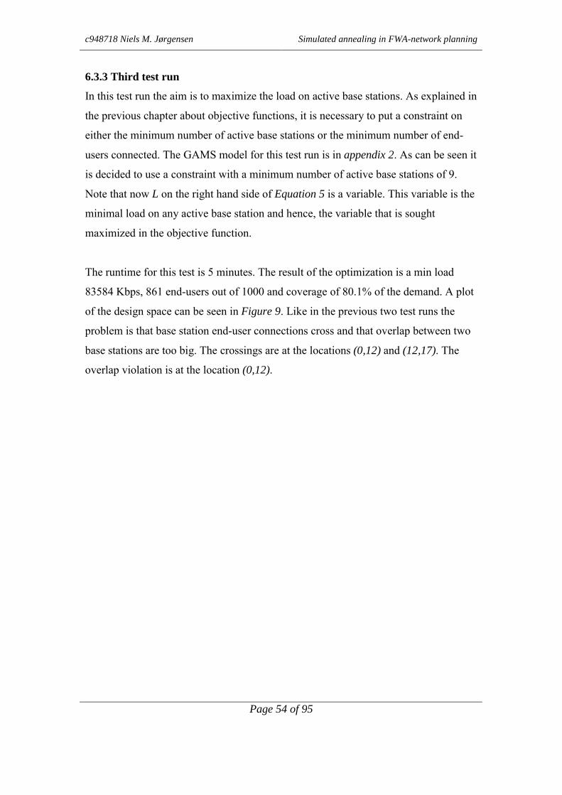
c948718 Niels M. Jørgensen Simulated annealing in FWA-network planning
Page 54 of 95
6.3.3 Third test run
In this test run the aim is to maximize the load on active base stations. As explained in
the previous chapter about objective functions, it is necessary to put a constraint on
either the minimum number of active base stations or the minimum number of end-
users connected. The GAMS model for this test run is in appendix 2. As can be seen it
is decided to use a constraint with a minimum number of active base stations of 9.
Note that now L on the right hand side of Equation 5 is a variable. This variable is the
minimal load on any active base station and hence, the variable that is sought
maximized in the objective function.
The runtime for this test is 5 minutes. The result of the optimization is a min load
83584 Kbps, 861 end-users out of 1000 and coverage of 80.1% of the demand. A plot
of the design space can be seen in Figure 9. Like in the previous two test runs the
problem is that base station end-user connections cross and that overlap between two
base stations are too big. The crossings are at the locations (0,12) and (12,17). The
overlap violation is at the location (0,12).

c948718 Niels M. Jørgensen Simulated annealing in FWA-network planning
Page 55 of 95
Figure 9
6.3.4 Fourth test run
In this test run the aim is to minimize the number of active base stations while
maintaining a fixed number of end-users connected. The GAMS model used for this
test run can be seen in appendix 3. The difference from the previous test runs is that
here is Equation 5 removed, which means that there is no minimum limit of the load
on active base stations. As objective function Equation 3 that minimizes the number
of active base stations is used. Furthermore, a constraint has been added the model
that controls that the minimum number of end-users connected is greater than 800.
The runtime for this test is 5 minutes. The result of the optimization is a solution with
7 base stations where the minimum load on an active base station is 66.449. 65.5% of
the demand is covered and the number of connected end-users is equal to the

c948718 Niels M. Jørgensen Simulated annealing in FWA-network planning
Page 56 of 95
constraint minimum limit of 800. A plot of the solution can be seen in Figure 10. In
this solution there is no connections that cross. However, a number of end-users are
connected to base stations that are different from the nearest base station to the end-
user. Furthermore, the base station at location (15,15) is significantly smaller than its
neighbors, which means that interference at end-users connected to this base station is
very likely to occur.
Figure 10
6.4 Relaxed exact model test run discussion
Generalizing the results of the test runs the major problem using this model is that
end-users do not get connected to the nearest base station. Moreover, the difference in
size in coverage area between overlapping base stations together with the overlap
itself are likely to introduce too much of interference. These problems are naturally

c948718 Niels M. Jørgensen Simulated annealing in FWA-network planning
Page 57 of 95
caused by the absence of the non-linear constraints. Following the three-step iterative
model explained in the beginning of this section would probably provide a good
useable solution. However, the number of cij-variables that are causing problems is
relatively large. In this situation more than 3 is considered ‘large’ due to the fact that
finding a solution for each combination of settings of these, say, 4 cij-variables
requires computation of 24 = 16 solutions. In all four test runs the computing time for
one solution were approximately 5 minutes. Therefore, the computing time for 16
solutions would exceed the time limit, of one hour, for this optimization. This minor
overrun of the time limit is possible to solve by splitting the problem onto two
computers. However, the number of ‘trouble making’ cij-variables is more likely to be
counted in tens or hundreds rather than ones. Resulting in a growth in computing
time, which is not possible to overcome with realistic investment in computer
hardware.
The obvious question now is if it is possible to improve the model in order to provide
better solutions faster. Considering the reason for the non-linearities, the essence is
that connecting end-users to base stations is dependent on the set of active base
stations. Moreover, simply connecting the end-users to the nearest base station could
set the variables identifying the connection between end-users and base stations.
However, it has not been possible to find either one linear equation or a set of linear
equations to perform this task.
Test runs of a relaxed model minimizing a cost function were also performed.
However, the run time for these tests were several days and the results were similar to
those illustrated in test run one to four.
At the end of the project period a minor error in the model was discovered. In real life
the end-user antenna is directed toward the base station that the end-user is assigned
to. Hence, the signal C/I-computation at each end-user must be made with respect to
this orientation and the associated antenna gain diagram. However, this error does not
make any difference in the conclusion on using the exact model. Taking the

c948718 Niels M. Jørgensen Simulated annealing in FWA-network planning
Page 58 of 95
orientation into account would add equations utilizing sinus and cosine functions to
the model and hereby making the model even harder to solve.
6.5 Relaxed exact model test run conclusion
In consequence of the results of the test runs and the following discussion, it must be
concluded that it is not possible to solve the base station location problem, within the
given time frame using the exact models described in the section ‘4 Mathematical
model‘.

c948718 Niels M. Jørgensen Simulated annealing in FWA-network planning
Page 59 of 95
7 Metaheuristic method
Due to the lack of success in using an exact method the natural step is to use a
heuristic method. A heuristic method is a structured way of finding good solutions. In
the actual case the largest advantage with the heuristic is that it has no problems
handling discrete variables and/or non-linear constraints.
One group of heuristics is called Metaheuristics. These heuristics outline solution
search methods in sufficiently general terms in order to make it possible to adapt the
heuristic to be able to find solutions to almost any optimization problem. The most
common Metaheuristics are Genetic algorithms, Taboo search, Guided local search
and Simulated annealing.
Apart from Genetic algorithms, these Metaheuristic methods work the following way.
Select a setting of variables that identifies the solution and evaluate this solution. Find
a new solution in the neighborhood, evaluate and compare this solution with the
previous solution and the best solution. This continues for a ‘large’ number of
solutions. The neighborhood is defined as the group of solutions that can be reached
from the actual solution using one move only. The factor that makes the largest
difference between Metaheuristics is the way moves are made. All the mentioned
Metaheuristics are descent-search algorithms. If the algorithm only moves to better
solutions it is most likely to end up in a local minimum which is not the global
minimum. The way to avoid this problem differs the last three heuristics, Taboo
search, Guided local search and Simulated annealing.
The idea of Taboo search is to store the latest g solutions visited, in the taboo list. In
each iteration the algorithm evaluates all solutions in the neighborhood of the current
one, and then moves to the best of these solutions not in the taboo list.
For using Guided local search a set of undesired features in the solution is needed.
Each time the algorithm finds a solution with one of the undesired features the
solution is penalized, hereby pushing the algorithm away from this solution.

c948718 Niels M. Jørgensen Simulated annealing in FWA-network planning
Page 60 of 95
Simulated annealing finds a neighborhood solution using a random function. If the
neighborhood solution is better than the actual solution, the algorithm moves to that
solution. If the neighborhood solution is worse, the algorithm moves to that solution
with a given probability. The value for controlling the probability is called a
temperature. The temperature is reduced over time, hereby reducing the probability of
moving to a worse solution.
Genetic algorithms are inspired by biological evolution and hereby the name. The
algorithm works with a population of solutions instead of single solutions. These
solutions mix and ‘breed children’ solutions that hopefully inherit their ‘parents’ good
solution features and develop even better solution features by mutations. Good
‘children’ solutions are added the population and an equal number of bad solutions
leave the population. This process continues over many generations of solutions and
hereby develops good solutions.
In any of the Metaheuristics, evaluation of a ‘large’ number of solutions is required.
Hence, in order to be able to go through ‘sufficiently many’ solutions within
‘reasonable’ time the Metaheuristics require a very fast method for setting, evaluating
and comparing each new solution with the actual solution. In the current case
‘reasonable’ time is one hour like for the exact model. ‘Sufficiently many’ is critical
in the attempt to get a good solution. However, it is only possible to make the perfect
setting of the parameter ‘number of solutions evaluated’ if the best solution found can
be compared with the optimal solution. As mentioned earlier the optimal solution is
extremely hard to find for the actual problem.
In this first attempt to use a heuristic it is decided to use Simulated annealing. This is
due to observed ability to produce good solutions in other problems combined with
the easy implementation of this heuristic. Besides it is assumed that the evaluation is
relatively hard and therefore it is attractive to use a heuristic that require few
evaluations for each move.

c948718 Niels M. Jørgensen Simulated annealing in FWA-network planning
Page 61 of 95
Before setting up the heuristic the following definitions have to be made.
- Problem representation
- Start solution
- Neighborhood
- Solution evaluation
- Cooling scheme
- Stop criterion
7.1 Problem representation
The design of the problem representation is made with focus on ease of computing.
The straightforward method is to use the model concept from the exact model. In the
exact model the number of variables is in the worst case roughly the number of base
stations multiplied by the number of end-users. A large number of these variable
combinations are illegal. For instance, each end-user can only be connected to one
base station and base stations cannot cover end-users that are farther away from the
base station than the maximal transmission distance. When generating a random start
the risk of generating an illegal solution is large. Hence, there is a risk of wasting time
on evaluating illegal solutions. Alternatively, building up a solution while performing
simultaneous check of the legality can be computationally demanding. Therefore the
result may be that the number of legal solutions evaluated is the same as if allowing
generation of illegal solutions. Hence, it seems potentially profitable to reconsider the
model of the network aiming for a solution representation that is easy to evaluate.
This model does not necessarily need to be absolutely equivalent to the exact model
though it must provide a solution that is legal with respect to this exact model.
7.1.1 Graph models
Inspired by article [2] the legal connections between base stations and end-users can
be described as a network Figure 11. This network is a bipartite graph with base
stations on one side and end-users on the other. Edges between base stations and end-
users are legal connections i.e. an edge connects an end-user with a base station if it is
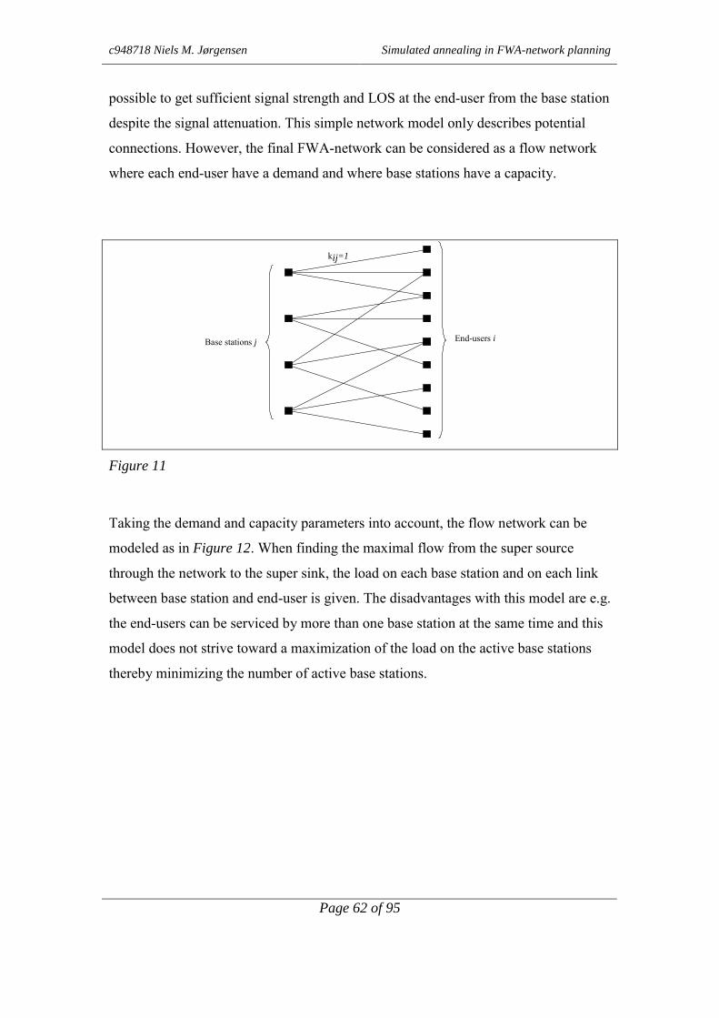
c948718 Niels M. Jørgensen Simulated annealing in FWA-network planning
Page 62 of 95
possible to get sufficient signal strength and LOS at the end-user from the base station
despite the signal attenuation. This simple network model only describes potential
connections. However, the final FWA-network can be considered as a flow network
where each end-user have a demand and where base stations have a capacity.
Base stations j End-users i
kij=1
Figure 11
Taking the demand and capacity parameters into account, the flow network can be
modeled as in Figure 12. When finding the maximal flow from the super source
through the network to the super sink, the load on each base station and on each link
between base station and end-user is given. The disadvantages with this model are e.g.
the end-users can be serviced by more than one base station at the same time and this
model does not strive toward a maximization of the load on the active base stations
thereby minimizing the number of active base stations.

c948718 Niels M. Jørgensen Simulated annealing in FWA-network planning
Page 63 of 95
Capacity at basestation j
Demand atend-user i
Unlimitedcapacity
Supersource
Super sink
Figure 12
Both Figure 11 and Figure 12 give inspiration to formulate the algorithm that
connects end-users to base stations.
Consider the non-linear constraint in Equation 9 controlling that the C/I-value at each
end-user is above a threshold value. It is easy to see that the greater the carrier signal
and the smaller the interfering signals the better is the C/I relationship. Increasing
output power at one base station will result in increased carrier signal at the end-users
that are connected to that base station and increased interfering signal at end-users not
connected to that base station. Connecting end-users to base stations is practically the
same as setting the power output level at the base station. To be able to reach an end-
user further away from the base station the output power has to be increased. The
output power at a base station can only be increased up to the hardware limit of the
output power. As mentioned previously the output power measured in dB can be
converted to transmission distance using a linear function.
In the first attempt to create a way of generating solutions, end-users are connected to
the nearest base station if this base station have sufficient capacity available.
Otherwise it is attempted to connect the end-user to the second nearest base station if
possible else the third and so on until the end-user is either connected or the distance
to the nearest base station with available capacity is exceeding the maximal
transmission limit. If the distance to the nearest base station with vacant capacity is

c948718 Niels M. Jørgensen Simulated annealing in FWA-network planning
Page 64 of 95
exceeding the maximal transmission distance the end-user is not connected at all.
When connecting end-users all end-users are sorted by the distance to their nearest
base station. The algorithm starts with the end-user with the shortest distance to a base
station. If an end-user cannot be connected to its nearest base station then the end-user
is placed in the list of non-connected end-users with the distance to its second nearest
base station. The list is then sorted again and the algorithm continues with the end-
user with the shortest distance to a base station.
This way of building up a solution ensures that the solution is legal with respect to the
transmission limit and the capacity limit. However, the solution is not necessarily
legal with respect to the interference limit but using the shortest possible distance
each time an end-user is connected, gives one of the best solutions with the given set
of base stations.
Finally, due to the unambiguous way of connecting end-users to base stations the
entire solution is given when a set of active base stations is selected.
7.2 Start solution
The initial solution is the starting point for the search for good solutions. In this
problem the initial solution can be given as a set of active base stations.
Depending on the target for the optimization the minimum number of active base
stations can be pre-computed. If all end-users must be connected, the minimum
number of active base station is the total demand divided by the capacity of the base
station rounded up to nearest integer. However, it is not certain that all end-user can
be connected using any set of base stations of this size or any other size due to
interference constraints.
The initial solution for this problem is found by a random selection of base stations.
End-users are connected to the selected base stations as indicated in the previous
section.

c948718 Niels M. Jørgensen Simulated annealing in FWA-network planning
Page 65 of 95
7.3 Neighborhood
The neighborhood is defined as the solutions that can be reached by one move from
the actual solution.
In this problem the neighborhood is defined as follows:
- One active base station is turned off and one inactive base station is turned on.
7.4 Solution evaluation
For a given solution it is necessary to be able to evaluate if the solution is better or
worse than the previous solution.
In this first attempt where illegal solutions are accepted the evaluation result in a
penalty. The penalties represent a cost on both the degree of constraint violations and
the network condition. See Equation 23. Each penalty is explained later in this
section. The penalty function is constructed as a linear sum of total cover circle
overlap, load deviation from a given minimum load on each base station if the load is
less than the minimum load, tapering between the coverage circle of two base stations
and the number of not connected end-users. In order to guide the solver toward a good
solution each penalty can be multiplied by a cost constant.
euconnNotoverlap
J
j
J
jkjkTapload QeuconnNotQolbsQTapQLoadPenalty __
1
1 1
___ ⋅+⋅+⋅+⋅=−
= +=
Equation 23
7.4.1 Circle overlap
The total circle overlap is computed as the sum of area of design space that is covered
by both base stations in any pair of active base stations. The formula for computing
this area is given by Equation 21.

c948718 Niels M. Jørgensen Simulated annealing in FWA-network planning
Page 66 of 95
7.4.2 Load deviation
The load deviation is the sum of difference between utilized capacity and a given
minimum load on base stations where the utilized capacity is less than the minimum
load ‘L’. Load deviation is computed using Equation 24.
IiLdcJjbdcLdeviationLoadi
ijijj i
iji ∈���
� <⋅∈⋅����
� ⋅−= ,, |_
Equation 24
7.4.3 Tapering
For any base station the distance to the most distant end-user identifies the radius of
the coverage circle. Tapering penalty is the sum of the relationships of the largest
radius over the smallest radius of any pairs of base stations where the following apply:
The sum of coverage radii rj and rk exceeds the distance between the base stations
distjk and the relationship of the largest radius over the smallest radius is greater than a
given constant. See the example in Figure 6. Here, if rj/rk is greater than a given
constant ‘K’ the relationship rj/rk is added the penalty. For convenience Figure 6 is
repeted below.
( )( )
( )( ) +ℜ∈
�
��
�
�>∧>+∈= KK
rrminrrmax
distbsrrJkjrrminrrmax
Taperingkj
kjkjkj
kj, kj
kj ;,,
_|,,,
,
Equation 25

c948718 Niels M. Jørgensen Simulated annealing in FWA-network planning
Page 67 of 95
b(j)b(k)
r(k)
l
r(j)
bs_dist(j,k)
θ(j)θ(k)
Figure 6
7.4.4 Not connected end-users
The number of not connected end-users are found using the following equation:
JjIicusersendconnectedNoti j
ji ∈∈�
���
�−=− ;1 ,
Equation 26
7.5 Cooling scheme
The cooling scheme indicates how the temperature is going to be reduced over time
and hereby reducing the probability of going to a solution worse than the actual
solution.
The easiest cooling scheme is to reduce the temperature by it with a constant after a
specified number of moves. The result of this is a logarithmic temperature curve. The
optimization is then done by performing a fixed number of iterations at each
temperature level until the stop criterion is reached. However, when the temperature is
high the algorithm accepts more or less all neighborhood solutions and performs no
actual descent search. Hence, in some cases it can be desirable to reduce the
temperature at a faster rate when the temperature is high. Using both ‘number of
accepted solutions’ and ‘a fixed number of evaluated solutions’ as criterion for

c948718 Niels M. Jørgensen Simulated annealing in FWA-network planning
Page 68 of 95
reducing the temperature can do this. The accepted number of solutions is naturally
lower than the fixed number of solutions.
At the end of the optimization it is essential that the temperature is not too low before
the stop criterion is reached. If the temperature is too low the algorithm will not
accept any ‘bad’ solutions at all and hereby making further search futile. One option
is to ‘reheat’ and hereby make it possible for the algorithm to accept ‘bad’ solutions
again.
In the actual case it is decided to use a simple cooling scheme. After evaluating a
fixed number of neighborhood solutions the temperature is lowered by multiplying
the temperature by a constant.
7.6 Stop criterion
The stop criterion decides the termination of the heuristic. The aim is to end the
heuristic when it is unlikely to find a new solution better than what is already found.
One option is to terminate the heuristic when it has been searching for ‘some time’
without finding any better solution. This can be done using a sliding window,
monitoring the number of accepted solutions over a number of iterations. If the
number of accepted solutions within the given number of iterations is less than a
threshold value the heuristic terminates. The disadvantage with this method is that it is
not possible to know prior to start of the heuristic how many iterations are needed
before termination and hereby determine how much time the optimization will take.
Another stop criterion is to terminate the heuristic after a fixed number of iterations.
This method requires a number of test runs in order to determine how many iterations
must be performed until the heuristic does not find any new better solutions within a
given ‘window’. Naturally, the point when the heuristic does not find any better
solutions is in some way dependent on the temperature. If the temperature is low and
the heuristic has been searching the local area for some time there is a good chance

c948718 Niels M. Jørgensen Simulated annealing in FWA-network planning
Page 69 of 95
that it has found the local minimum and cannot escape from there and therefore
cannot get to another local minimum.
Due to the fact that in the current case time is a critical parameter, it is decided to use
a stop criterion that terminates the heuristic after a fixed number of iterations. Hereby
is it possible prior to optimization to compute how long it takes until the heuristic
terminates.
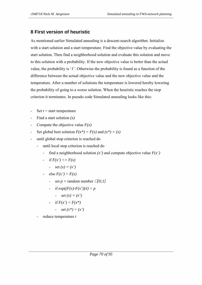
c948718 Niels M. Jørgensen Simulated annealing in FWA-network planning
Page 70 of 95
8 First version of heuristic
As mentioned earlier Simulated annealing is a descent-search algorithm. Initialize
with a start solution and a start temperature. Find the objective value by evaluating the
start solution. Then find a neighborhood solution and evaluate this solution and move
to this solution with a probability. If the new objective value is better than the actual
value, the probability is ‘1’. Otherwise the probability is found as a function of the
difference between the actual objective value and the new objective value and the
temperature. After a number of solutions the temperature is lowered hereby lowering
the probability of going to a worse solution. When the heuristic reaches the stop
criterion it terminates. In pseudo code Simulated annealing looks like this:
- Set t = start temperature
- Find a start solution (x)
- Compute the objective value F(x)
- Set global best solution F(x*) = F(x) and (x*) = (x)
- until global stop criterion is reached do
- until local stop criterion is reached do
- find a neighborhood solution (x’) and compute objective value F(x’)
- if F(x’) <= F(x)
- set (x) = (x’)
- else F(x’) > F(x)
- set p = random number ∈ [0;1]
- if exp((F(x)-F(x’))/t) < p
- set (x) = (x’)
- if F(x’) < F(x*)
- set (x*) = (x’)
- reduce temperature t

c948718 Niels M. Jørgensen Simulated annealing in FWA-network planning
Page 71 of 95
8.1 Testing the Metaheuristic
The Metaheuristic is implemented in C. The visualization of the result is made using
functions developed in the program Matlab . The data set used for the test run is the
same as those used in the exact case.
8.2 Parameter setting
The following parameters must be set prior to perform the test run:
- Start temperature
- End temperature
- Cooling rate
- Number of local iterations
- Number of global iterations
All five parameters are in some way related to each other. In the current case the
optimization must be performed within the given timeframe of one hour. When the
time/iteration is known it is simple to determine how many iterations can be
performed within this given timeframe. Let ‘TI’ indicate the total number of iterations
that can be performed. After TI iterations the temperature must be reduced from the
start temperature to the end temperature.
Start and end temperatures are relatively easy to find using the following procedures.
In order to make a good search of the solution space the start temperature must be set
at a level where the heuristic accepts many of the generated solutions. This regardless
that for each pair of new and actual solutions the new solution can be worse than the
actual one. In literature about simulated annealing [8] accept rates at 50-70% of all
generated solutions is considered to be sufficient for a good search. For finding the
start temperature a first guess of the temperature is made, then 10 test runs with 100
solutions generated in each is made and the average number of accepted solutions in
those 10 times 100 solutions are computed. Then the temperature is adjusted and 10
more test runs are made. This is continued until the number of accepts is satisfactory.

c948718 Niels M. Jørgensen Simulated annealing in FWA-network planning
Page 72 of 95
When setting the end temperature the task is to ensure that time is not wasted by
performing search for solutions when the end temperature is too low to accept any
worse solutions at all. However, the end temperature must not be set so high that the
heuristic does not perform a thorough search of the neighborhood before terminating.
The way of finding the end temperature is to perform a test run where the end
temperature is set very low. The setting of the end temperature is then found by a
visual inspection of a plot of the actual objective value at each iteration. The end
temperature is the temperature at the time where the actual objective value has not
changed for ‘some time’.
Note that the start and end temperatures are dependent on the numerical size of the
difference between the actual and the new objective value. Hence, if the evaluation
function is changed it is important to check that the start and end temperatures still are
right.
Local iteration is the number of iterations that are performed at each temperature
level. Global iteration is the number of times the temperature must be reduced in
order to go from start temperature to end temperature. See Equation 27. Hence, global
iteration multiplied by local iteration must be equal to TI.
etemperaturEndratecoolingetemperaturStart iterationglobal ___ _ =⋅
Equation 27
The combination of cooling rate, global iteration and local iteration can be anything
from TI local iterations at start temperature and only one temperature drop to end
temperature, to one local iteration at each temperature level and reducing the
temperature TI times. This is possible as long as the product of global and local
iterations is equal to TI.
The relation between start temperature, end temperature, cooling rate and global
iteration can be expressed by Equation 28.

c948718 Niels M. Jørgensen Simulated annealing in FWA-network planning
Page 73 of 95
( )ratecoolLnetemperaturStartetemperaturEndLn
iterationglobal_
__
_
����
�
=
Equation 28
Setting the size of local iteration must be done with some respect to the size of the
neighborhood. Prior to termination the heuristic must be allowed a good probability
that the algorithm finds the minimal solution in the neighborhood. The number of
solutions in the neighborhood in the actual case is the number of active base stations
multiplied by the number of inactive base stations. Hence, identifying the number of
iterations that are sufficient for a good probability must be done by performing a
number of test runs where different settings of global and local iterations, combined
with the appropriate cooling rates are tested.
8.2.1 Cooling rate
The typical value for cooling rate is between ‘0.94’ and ‘0.98’ and initially the value
‘0.96’ is selected.
8.2.2 Global iteration
When start temperature, end temperature and cool rate are decided, global iteration is
simple to compute using Equation 28:
8.2.3 Local iteration
The local iteration is set in accordance with the results of the test runs, mentioned
earlier.
8.3 Test run of first version
The result of the first test run can be seen in Figure 13. A visual inspection of the
result unveils that this solution is not sufficiently good. This is due to the violation of
the two constraints, tapering and overlap.

c948718 Niels M. Jørgensen Simulated annealing in FWA-network planning
Page 74 of 95
Figure 13
Two obvious violations of the tapering constraint appear in the solution. At location
(14,15) is a base station located with transmission radius significantly smaller than its
neighbors. Similarly at location (2,20) is the difference in transmission radii.
The overlap constraint is violated at least 5 times. At the locations (2,20), (2,13),
(5,13), (12,18) and (14,15) the overlap between neighboring transmission areas is too
big. At other locations there appears to be violations too but they are not obvious
cases.
Additionally, another undesired design error appears. At location (2,11) a number of
the lines indicating end-user-base station connections cross each other. The result of
these crossing is interference and furthermore it is easy to see that if the two end-users
swap base station the crossing is removed and, in special cases, the need for

c948718 Niels M. Jørgensen Simulated annealing in FWA-network planning
Page 75 of 95
transmission power could be reduced. Finally, these crossings indicate that the
algorithm that connects end-users to base stations is not good enough.
Fitting the weights related to each constraint violation could probably solve the
trouble with the overlap and tapering. However a number of test runs has been
performed with high penalty on overlap and low penalty on tapering, with low penalty
on overlap and high on tapering and one test run with high penalty on both tapering
and overlap. The results of these test runs showed that it is possible to reduce either
tapering, overlap or both. However, the adequate setting of the costs related to the
constraints violations are hard to find. Moreover, due to the problems with the
connections that cross, the construction of this heuristic is reconsidered. This gave rise
to a number of changes and improvements to the heuristic.

c948718 Niels M. Jørgensen Simulated annealing in FWA-network planning
Page 76 of 95
9 Second version of heuristic
In this version the problem representation is equal to the representation in the
previous. Moreover, in this heuristic only legal solutions are generated. When a set of
base stations is found the end-user base station connections are unambiguously given.
The overlap expressed in Equation 18 is demanding to compute. Due to the fact that,
in this version, the check must be performed each time a new end-user is attempted
connected, the overlap must be computed one time for each combination of base
stations and end-users. In order to keep the computing time low we use a more simple
function of the overlap that is not so computationally demanding. We use simple
overlap as a constraint instead. The constraint is explained later in this section.
In this version a solution is constructed in the following way:
- find a set of base stations
- find nearest active base station for each end-user
- Connect end-users to base stations starting with the shortest end-user base station
connection then the second shortest and so on.
Before each end-user is connected a number of checks have to be performed to ensure
that the solution still is legal when the actual end-user have been connected. The
checks performed are the following:
- Max. transmission distance.
- Max. base station capacity.
- Maximal simple overlap between the actual base station and all neighboring base
stations.
- Maximal tapering difference between the actual base station and all neighboring
base stations.
If the end-user exceeds the limits in either one of the checks the end-user is not
connected at all. The heuristic then proceeds to the next end-user.

c948718 Niels M. Jørgensen Simulated annealing in FWA-network planning
Page 77 of 95
9.1 New constraints
9.1.1 Maximal simple overlap
For a given solution where some or all end-users have been connected the distance to
the most distant end-user at each base station identify the current radius of the
coverage circle. The distance between any two base stations must not be less than a
given percentage of the sum of the covering radii of the base stations. See the example
in Figure 6. Here the sum of rk and rj multiplied by a percentage, K, must be less than
the distance between the base stations bs_distj,k.
( ) [ ]0;1KJkjdistbsKrr kjkj ∈∈∀<⋅+ ;,_ ,
Equation 29
9.1.2 Tapering
Tapering in this version is similar to the tapering in the previous version. However in
this version the constraint is formulated slightly different due to the fact that here it is
used as a bound instead of a penalty. See Equation 30. In this version the tapering
constraint is formulated in a way where the latest end-user-base station connection is
legal if the following apply. For any pair of the actual connecting base station and all
other base stations, the smallest radius is greater than the largest radius multiplied by
a constant.
( ) ( ) ( ) [ ]0;1K2distbs
rrmaxJkjrrmaxKrrmin kjkjkjkj ∈>∈∀⋅> ;
_,|,,, ,
Equation 30
In this case the tapering constraint does not apply for any pair of base stations when
the algorithm starts. If end-users were evenly distributed it would cause no problem to
connect end-users the way used in this version. This is due to the fact that coverage
circles then would ‘grow’ at almost the same rate. At the point when two circles starts
to overlap they are almost the same size. In the actual problem end-users can be
distributed in any fashion. Consider a situation where the border between a densely
populated area and a sparsely populated area is narrow see Figure 14. Because the

c948718 Niels M. Jørgensen Simulated annealing in FWA-network planning
Page 78 of 95
end-user that is about to be connected is the one with the shortest distance to a base
station the cover circles at base station j and k will have approximately the same size
when base station k have no more vacant capacity. As the process of connecting end-
users continues the size of the coverage radius at base station j grows. Naturally no
end-user located on the right side of the center normal can be connected to base
station j due to the fact that end-users must only connect to the nearest base station.
Therefore no end-user located at the right side of the center normal can induce a cover
circle on base station j exceeding the center normal. End-users located on the left side
of the center normal but more distant from the base station than the center normal, can
be connected to base station j. Hereby this or these end-users induce a cover circle
that also cover parts of the area to the right of the center normal. If the check of
tapering is made only when circles overlap then the solution is already illegal. Hence,
it is decided to make the tapering check when at least one of the cover radii exceeds
the center normal.
center normal
Dense populated area
Sparsely populated area
Base station j
Base station k
Figure 14
9.2 Neighborhood
In this heuristic the neighborhood is defined as in the first version of the heuristic.
- One active base station is turned off and one inactive base station is turned on.

c948718 Niels M. Jørgensen Simulated annealing in FWA-network planning
Page 79 of 95
Furthermore, it is decided to extend the neighborhood by adding the following two
operations:
- One active base station is turned off
- One inactive base station is turned on.
These two operations change the final number of base stations. In some cases it is
desirable to be able to control the final number of base stations. Hence, these two
operations can be set inactive. If they are active a random process controls which one
of all three operations that is used in a given iteration.
9.3 Evaluation
In this version of the heuristic like in the previous version the evaluation is initially
based on the number of not connected end-users. The function for finding the number
of not connected end-users is Equation 26. The aim of this optimization is to find a
solution where a minimal number of end-users are not connected.
In this version of the heuristic three additional options for optimization is added.
These options are minimal sum of not connected demand and minimal sum of either
not connected demand or end-users weighted by a density measuring. In Equation 31
is the general equation for the objective function. If neither demand, weight nor both
are desired in the solution the respective variables, di and wi, are set equal to 1.
JjIiwdc-1demandweighted iii j
ij ∈∈∀⋅⋅�
���
�= ,_
Equation 31
The density weight is made the following way. Design space is tiled into a 20 times
20 grid that makes the boundaries for the density measuring. The demand or number
of end-users in each tile is summed. These 400 values are normalized by dividing the
each value by the largest value and added a constant of ‘0.5’. The result is a value in
the interval [0.5;1.5] for each of the 400 tiles. When computing the objective value

c948718 Niels M. Jørgensen Simulated annealing in FWA-network planning
Page 80 of 95
each not connected end-user or demand is multiplied by the weight of the tile where
the end-user is located.
The advantages using these weights in the objective function is that the heuristic
strives toward a solution where covering densely populated areas have a higher
priority than covering sparsely populated areas. This is in line with desires expressed
by operators.
9.4 Test run of second version
The aim with the test run with this second version of the heuristic is the following:
- Does the improvements actually make the heuristic able to provide a good
solution?
- What is the best setting of the parameters cooling rate, local iteration and global
iteration?
- What is best: many short optimizations or one long optimization?
- Can the heuristic provide a good solution when setting the number of base stations
itself?
- How long time does the heuristic need in order to find the best solution?
The data used in the test runs are the same as used in the exact algorithm or chosen
the same way. The following settings have been used in the test runs.
- Tapering constant: 0.70
- Overlap constant: 0.70
The C-program source code of the heuristic can be seen in appendix 8.
Initial tests were performed on four different computers in order to measure the
performance in run time. The results of the evaluations/second test are the following:

c948718 Niels M. Jørgensen Simulated annealing in FWA-network planning
Page 81 of 95
Processor Operation System Evaluations/second
Pentium I 100, MHz Win 95 OSR2 2
Pentium II, 266 MHz Win NT4 24
Athlon 933 MHz Win 2000 39
Pentium III, 800 MHz Win NT4 112
Table 1
Using the Pentium III, 800 Mhz computer it is possible to perform an evaluation of
approximately 360.000 solutions within the given timeframe of one hour for the given
problem size.
9.4.1 Does the improvements actually make the heuristic able to provide a good
solution?
This test run is made using the test ‘test0’, the same as in the exact case. In order to be
able to compare the results with the results from the exact attempt these optimizations
are performed with 7 and 9 base stations. The optimizations are performed by
minimizing the number of not connected end-users, like in the exact cases ‘First test
run’ and ‘Second test run’.
A plot of the result of the test run in the case with 7 base stations can be seen in
Figure 15. Details about the settings of the heuristic can be seen in appendix 4. The
number of not connected end-users in this solution is 272 and the minimal load on a
base station is 64.512 kbps. The values in the exact case are respectively 250 and of
course 96.000.

c948718 Niels M. Jørgensen Simulated annealing in FWA-network planning
Page 82 of 95
Figure 15
A plot of the result of the test run in the case with 9 base stations can be seen in
Figure 16. Details about the settings of the heuristic can be seen in appendix 5. Here
the number of not connected end-users is 198 and the minimal load on a base station
is 40.832 kbps. The values in the exact case are 110 and 50.496, respectively.
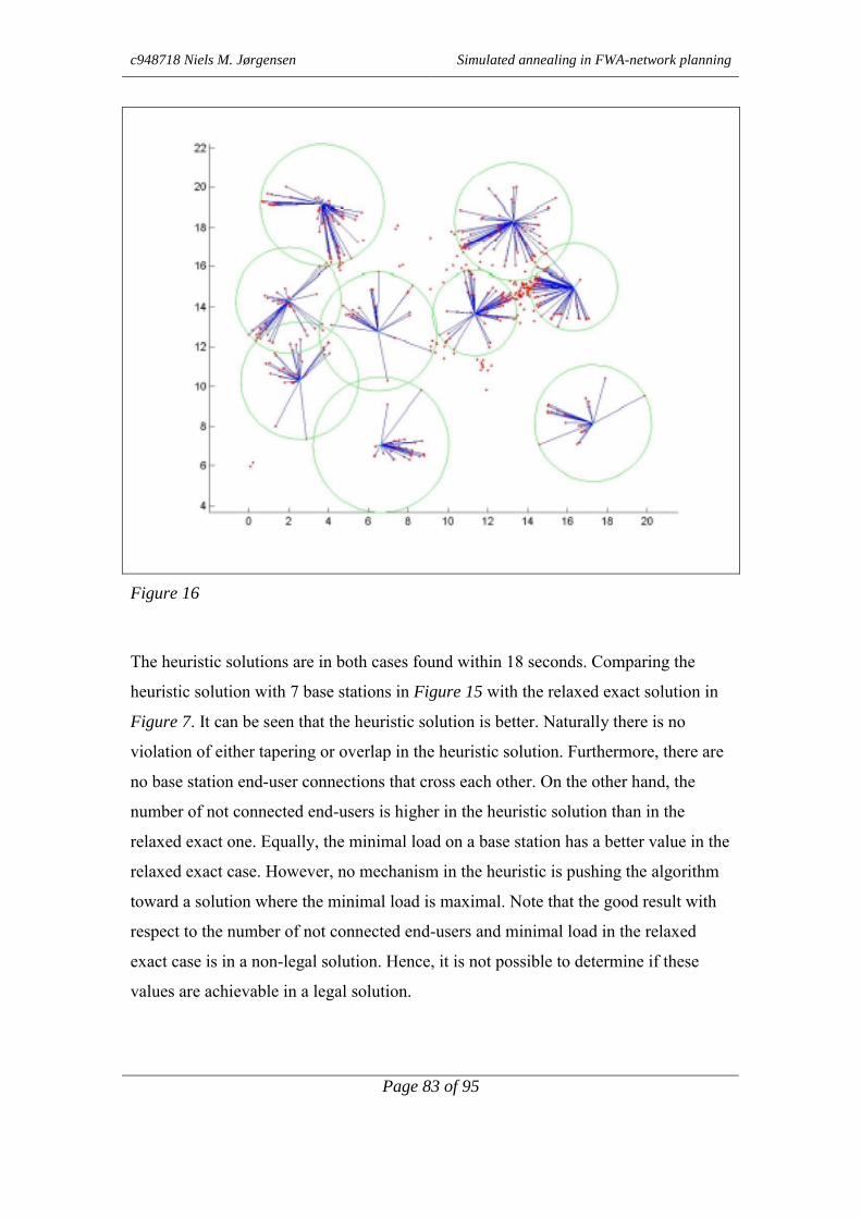
c948718 Niels M. Jørgensen Simulated annealing in FWA-network planning
Page 83 of 95
Figure 16
The heuristic solutions are in both cases found within 18 seconds. Comparing the
heuristic solution with 7 base stations in Figure 15 with the relaxed exact solution in
Figure 7. It can be seen that the heuristic solution is better. Naturally there is no
violation of either tapering or overlap in the heuristic solution. Furthermore, there are
no base station end-user connections that cross each other. On the other hand, the
number of not connected end-users is higher in the heuristic solution than in the
relaxed exact one. Equally, the minimal load on a base station has a better value in the
relaxed exact case. However, no mechanism in the heuristic is pushing the algorithm
toward a solution where the minimal load is maximal. Note that the good result with
respect to the number of not connected end-users and minimal load in the relaxed
exact case is in a non-legal solution. Hence, it is not possible to determine if these
values are achievable in a legal solution.

c948718 Niels M. Jørgensen Simulated annealing in FWA-network planning
Page 84 of 95
Finally, a solution evaluation that is closer to real life has been developed. This
evaluation computes the C/I ratio at each end-user with respect to the end-user
antenna diagram. The number of end-users that has a C/I ratio greater than 22 dB is
680 in the case with 7 base stations. In the case with 9 base stations the number of
end-users with a C/I ratio that is greater than 22 dB is 693. These two results are
considered realistic by Senior specialist, Phd. Christian Kloch at L.M. Ericsson,
Denmark. The function used for computing the C/I ration and the antenna diagram
can be seen in appendix 6.
9.4.2 What is the best setting of the parameters cooling rate, local iteration and
global iteration?
For finding the best setting of the parameters cooling rate and local and global
iteration, the following test is performed:
Four test runs each with different seed value are performed. In each run one
optimization is performed using each cooling rate from the set {0.91, 0.92…0.98,
0.99}. The total number of iterations in each of the optimizations is selected to be
2000. Hence, the optimization can be performed within 20 seconds. The number of
global iterations is computed by the program itself using Equation 28. The number of
local iterations is also computed by the program as the total number of equations
divided by the number of global iterations. Both iteration numbers are naturally
rounded to nearest integer value. Hence, the effective total number of iterations in
each test run is different from 2000 and is in the range [1748;1988]. The data set for
the test run is ‘Test0’. The result of the test run can be seen in Figure 17. Here the
average of the objective values at each cooling rate is illustrated relative to the total
average of all objective values from all cooling rates.
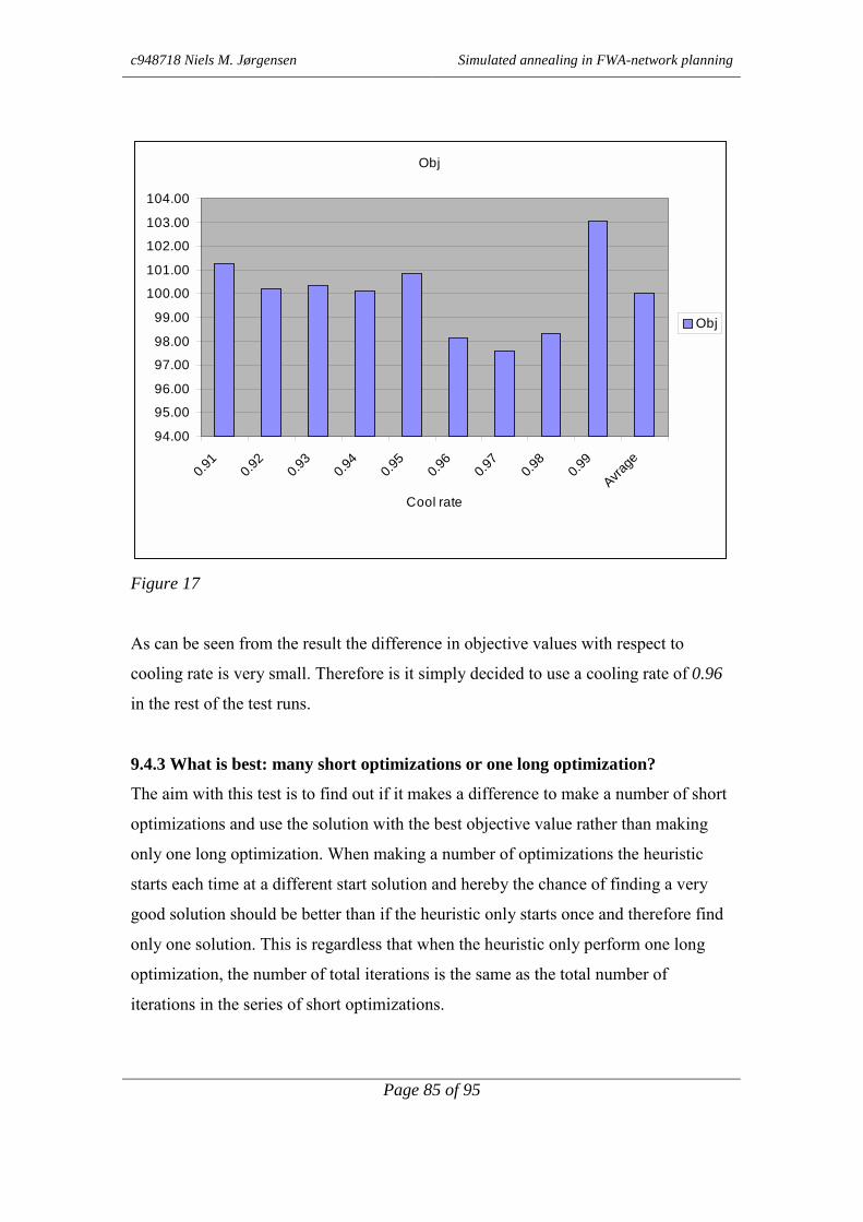
c948718 Niels M. Jørgensen Simulated annealing in FWA-network planning
Page 85 of 95
Obj
94.00
95.00
96.00
97.00
98.00
99.00
100.00
101.00
102.00
103.00
104.00
0.91
0.92
0.93
0.94
0.95
0.96
0.97
0.98
0.99
Avrage
Cool rate
Obj
Figure 17
As can be seen from the result the difference in objective values with respect to
cooling rate is very small. Therefore is it simply decided to use a cooling rate of 0.96
in the rest of the test runs.
9.4.3 What is best: many short optimizations or one long optimization?
The aim with this test is to find out if it makes a difference to make a number of short
optimizations and use the solution with the best objective value rather than making
only one long optimization. When making a number of optimizations the heuristic
starts each time at a different start solution and hereby the chance of finding a very
good solution should be better than if the heuristic only starts once and therefore find
only one solution. This is regardless that when the heuristic only perform one long
optimization, the number of total iterations is the same as the total number of
iterations in the series of short optimizations.
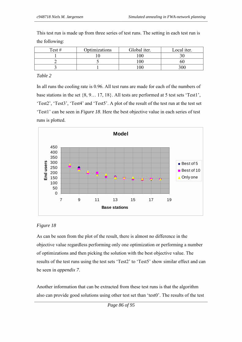
c948718 Niels M. Jørgensen Simulated annealing in FWA-network planning
Page 86 of 95
This test run is made up from three series of test runs. The setting in each test run is
the following:
Test # Optimizations Global iter. Local iter.1 10 100 302 5 100 603 1 100 300
Table 2
In all runs the cooling rate is 0.96. All test runs are made for each of the numbers of
base stations in the set {8, 9… 17, 18}. All tests are performed at 5 test sets ‘Test1’,
‘Test2’, ‘Test3’, ‘Test4’ and ‘Test5’. A plot of the result of the test run at the test set
‘Test1’ can be seen in Figure 18. Here the best objective value in each series of test
runs is plotted.
Model
050
100150200250300350400450
7 9 11 13 15 17 19
Base stations
End
user
s Best of 5Best of 10Only one
Figure 18
As can be seen from the plot of the result, there is almost no difference in the
objective value regardless performing only one optimization or performing a number
of optimizations and then picking the solution with the best objective value. The
results of the test runs using the test sets ‘Test2’ to ‘Test5’ show similar effect and can
be seen in appendix 7.
Another information that can be extracted from these test runs is that the algorithm
also can provide good solutions using other test set than ‘test0’. The results of the test

c948718 Niels M. Jørgensen Simulated annealing in FWA-network planning
Page 87 of 95
runs in the test sets ‘test1’ to ‘test5’ is a number of not connected end-users in the set
{140, 141…280, 281}.
Note that a series of optimizations as this provides a 2-criterion solution. For each
setting of the number of base stations the heuristic provides a number of not
connected end-users.
9.4.4 Can the heuristic provide a good solution when setting the number of base
stations it self?
The aim with this test is to see if it is possible for the heuristic to find a good solution
when setting the number of base stations it self, in order to minimize the number of
not connected end-users. In the previous tests the number of base stations has been
pre-set. However, the pre-set can only be made on the basis of guess or a desire for a
specific number of base stations. If the objective is to find the solution with the
overall minimal number of not-connected end-users regardless the number of base
stations, the number of base stations can be found by doing a series of optimizations.
In each optimization using a number of base stations from the set {1,2…(|J|-1), |J|}.
Recall J is the set of potential base stations. However, some of the optimizations can
be omitted if the product of the number of base stations and base station capacity is
less than the minimal sum of demand that has to be connected.
Fortunately, in the previous test, 11 tests each with a number of base stations from the
set {8,9…17,18} has been made in each of the test sets ‘test1’ to ‘test5’. From Figure
18 it can be seen that the best solution among the performed optimizations is the one
with 16 base stations. Note this is not necessarily the best solution despite it appears
that way, for two reasons. First the optimization is made using a heuristic and second
there is a chance a better solution can be found using more than 18 base stations.
The test run where the heuristic is suppose to find the number of base stations itself is
performed using the test set ‘Test1’. The probability controlling which of the
following functions to use are initially set to:

c948718 Niels M. Jørgensen Simulated annealing in FWA-network planning
Page 88 of 95
- Only add base station 38/506
- Only remove base station 12/506
- Both add and remove base stations 456/506
The values are computed on the basis of the following values:
506 is the number of neighborhood solutions using all three neighborhoods where
the number of active base stations is 12.
12 is the number of neighborhood solutions when only removing base stations.
38 is the number of neighborhood solutions when only adding base stations.
456 is the number of neighborhood solution when both adding and removing base
stations.
An initial test run showed that the number of base stations increased to 50 active base
stations during the test run. The reason for this increase is probably that when the
heuristic tries to remove one base station it is very likely that the objective value of
the new solution is worse than the actual objective value. Hence, the heuristic rarely
removes a base station.
Instead the probabilities is tried to be set as follows:
- Only add base station 2.5%
- Only remove base station 5.0%
- Both add and remove base stations 92.5%
The number of global iterations is 100 and the number of local iterations is 60. Hence,
the total number of iterations is 6000. The numbers of base stations is found as part of
the test run while minimizing the number of not connected end-users. The result of
the test run can be seen in Table 3, together with the result where the number of base
stations is pre-set:

c948718 Niels M. Jørgensen Simulated annealing in FWA-network planning
Page 89 of 95
# of base stations Not connected end-usersfound # of base stations
Not connected end-userspre-set # of base stations
13 159 16715 146 14616 137 13717 147 13721 143 -
Table 3
Comparing the two columns with not connected end-users in Table 3 it can be seen
that the heuristics finds solutions with almost the same objective value.
It is worth noticing that the results in these test runs do not necessarily provide
solutions that are profitable for the practical base station location problem.
9.4.5 How long time does the heuristic need in order to find the best solution?
The aim whit this test run is to see how much does the solution improve with more
iterations. The test is performed at the test set ‘test1’ with 14 base stations and using a
total number of iterations from 500 to 6000 in steps of 500. A plot of the result can be
seen in Figure 19. As can be seen there is, as expected, a tendency toward better
solutions when performing more iterations. Though, with 29916 iterations the
objective value is worse than with 4968, 5400 and 5940 iterations! However, these
test runs were performed using a cooling rate of 0.96. If there is time to perform
several long optimizations more investigation in parameter setting can be
advantageous. Especially, the issues regarding cooling rate, utilization of accept rate
when temperature is high and utilization of reheat when temperature is low could be
beneficial to use.

c948718 Niels M. Jørgensen Simulated annealing in FWA-network planning
Page 90 of 95
obj
100
120
140
160
180
200
220
432
972
1404
1944
2484
2916
3456
3996
4428
4968
5400
5940
2991
6
total iterations
Not
con
nect
ed e
nd-u
sers
obj
Figure 19
9.5 Heuristic method test run discussion
According to the results in the tests described previously in this section it seems that
the second version of the Simulated annealing is able to perform optimizations using
the number of not connected end-users as optimizations parameter when the number
of base stations is fixed. Setting the number of base stations, as part of the
optimization process is also possible according to the results. However, more work
needs to be done if this heuristic shall provide solutions that are applicable in real life.
9.6 Heuristic method test run conclusion
As described in the discussion section the second version of Simulated annealing is
able to perform optimization using the number of not connected end-users as
optimization parameter with success within the given time frame.

c948718 Niels M. Jørgensen Simulated annealing in FWA-network planning
Page 91 of 95
10 General discussion
According to the section ‘relaxed exact model test run’ it is not possible to solve the
given problem using an exact method within the given time frame. Furthermore, there
does not appear to be any options for solving this problem without use of some sort of
heuristic method. Fortunately, according to the section ‘test run of second version’,
the method developed and implemented is able to place base stations and connect
end-users to these base stations. Moreover, the heuristic method is able to perform the
location of base stations and connecting end-users in less than 60 seconds. Hereby
making it possible to perform a number of optimizations in order to compare different
solutions.
Issues interesting for future testing could include the feature that provides the option
to weight the end-users according to the density of the area where they are located.
In the second version of the heuristic focus has only been on using the number of not
connected end-users as objective value. However, consider the results of the test runs
where setting the number of base stations is a part of the optimization. Here, other
parameters must be included in the objective function in order to make the heuristic
able to weight the marginal improvement of the end-user coverage when adding or
removing base stations.
The exact method has the option of optimizing the maximal minimal load on active
base stations. This feature is not optional in the heuristic in the current version.
However, it appears to be worth consider a function that makes it possible to optimize
the network using the minimal load on a base station as objective function. Another
option is to use a linear sum of connected end-users and the minimal load on a base
station as an objective function. Implementation of these functions is assumed to
improve the commercial usability.

c948718 Niels M. Jørgensen Simulated annealing in FWA-network planning
Page 92 of 95
11 General conclusion
According to the section ‘General discussion’ and the conclusions in the section ‘Test
run of second version’, a method able to place base stations and connect end-users to
base stations, spending less than one hour, has been developed and implemented
successfully.

c948718 Niels M. Jørgensen Simulated annealing in FWA-network planning
Page 93 of 95
References
[1] Optimal Network Design: the Base Station Placement Problem
Shih-Tsung Yang and Anthony Ephremides
Institute for Systems Research and Electrical Engineering Department
University of Maryland, College Park
[2] Genetic Approach To Radio Network Optimization For Mobile Systems
Calégari P., Guidec F., Kuonen P., Wagner D.
EPFL Swiss Federal Institute of Technology, Dept. of Computer Science
1015 Lausanne, Switzerland
TDF-C2R Mobile communications and broadcasting research center
1, rue Marconi, 57070 Metz, France
[3] Radio network optimization with maximum independent set search
Chamaret B., Josselin S.,Kuonen P., Pizarroso M., Salas-Manzanedo B., Ubeda S.,
Wagner D.
TDF-C2R Mobile communications and broadcasting research center
1, rue Marconi, 57070 Metz, France
Ecole Normale Superieure De Lyon
46, allée d’Italie
69364 Lyon Cedex 07, France
EPFL Swiss Federal Institute of Technology, Dept. of Computer Science
1015 Lausanne, Switzerland
Telefonica I+D
Emilio Vargas, 6
E-28043 Madrid, Spain
[4] Base Station Location Optimization
Ivan Howitt and Seung-Young Ham
Wireless and Signal Processing Laboratory – EECS Department

c948718 Niels M. Jørgensen Simulated annealing in FWA-network planning
Page 94 of 95
University of Wisconsin – Milwaukee, PO Box 784, Milwaukee, WI 53201 USA
[5] Optimization Methods for Base Station Placement in Wireless Applications
Margaret H. Wright
Bell Laboratories, Lucent Technologies
Murray Hill, New Jersey 07974, USA
[6] Optimal location of transmitters for micro-cellular radio communication system
design
Hanif D. Sherali, Chandra Mohan Pendyala,
Department of industrial and systems engineering, Virginia Polytechnic Iinstitute and
State University, Blacksburg VA 24061-0118 USA
Theodore S. Rappaport
Department of elecrical engineering, Virginia Polytechnic Iinstitute and State
University, Blacksburg VA 24061-0118 USA
[7] Spectral Efficiency and optimal base placement for indoor wireless networks
Dimitris Stamatelos and Anthony Ephremides
Department of Electrical Engineering, University of Maryland, College Park 20742
USA
[8] General local search heuristics in Combinatorial Optimization: a tutorial.
M. Pirlot
Belgian journal of Operations Research,
Statistics and Computer Science, Vol. 32 no 1-2
[9] Matematisk modellering
Svend Clausen
IMM

Appendix 1
Full version can be found on CD\Exact1\cut_dk.gms
option iterlim=999999999, reslim=3600000, optcr=0.0;SET enduser End_user
/1*1000/;ALIAS(enduser,i);
SET Basestat Base stations/1*50/;ALIAS(Basestat,j,bs);
SET korr koordinater/X,Y/;ALIAS(korr,za);
TABLE lcbs(j,za)
X Y1 0.798745 13.1629662 14.740898 15.1952473 12.550226 18.088731
-- CUT --48 14.390101 15.41624849 16.453164 14.07679150 13.722607 15.214297;
TABLE lceu(i,za)
X Y1 0.798745 13.1629662 0.798745 13.1629663 13.933195 15.186057
-- CUT --998 1.994665 14.316662999 1.994665 14.3166621000 5.741703 17.338247;
TABLE k(i,j)1 2 3 4 5 6 7 8
9 10 11 12 13 14 15 16 17 1819 20 21 22 23 24 25 26 27 2829 30 31 32 33 34 35 36 37 3839 40 41 42 43 44 45 46 47 4849 50
1 1 0 0 0 0 0 0 00 1 0 0 0 0 0 0 0 00 0 0 0 1 0 0 0 1 00 0 0 0 0 0 0 1 0 00 0 0 0 1 0 0 0 0 00 0
2 1 0 0 0 0 0 0 00 1 0 0 0 0 0 0 0 00 0 0 0 1 0 0 0 1 00 0 0 0 0 0 0 1 0 00 0 0 0 1 0 0 0 0 00 0

3 0 1 0 0 1 0 0 00 0 0 1 0 0 0 0 0 00 0 0 0 0 0 0 0 0 01 0 0 0 0 0 0 0 0 00 0 1 0 0 0 0 0 0 10 1
4 0 0 0 0 0 1 0 00 0 0 0 0 0 0 0 0 00 0 0 0 0 0 0 0 0 00 0 0 1 0 0 0 0 0 00 0 0 0 0 0 0 0 0 00 0-- CUT --
997 1 0 0 0 0 0 0 00 1 0 0 0 0 0 0 0 00 0 0 0 1 0 0 0 1 10 0 0 0 0 0 0 1 0 00 0 0 0 1 0 0 0 0 00 0
998 1 0 0 0 0 0 0 00 1 0 0 0 0 0 0 0 00 0 0 0 1 0 0 0 1 10 0 0 0 0 0 0 1 0 00 0 0 0 1 0 0 0 0 00 0
999 1 0 0 0 0 0 0 00 1 0 0 0 0 0 0 0 00 0 0 0 1 0 0 0 1 10 0 0 0 0 0 0 1 0 00 0 0 0 1 0 0 0 0 00 0
1000 0 0 0 0 0 0 0 00 0 0 0 0 1 0 1 0 00 0 0 0 0 0 0 0 0 10 0 0 0 0 0 1 0 0 00 0 0 0 0 1 0 1 0 00 0;
PARAMETERdist(i,j);dist(i,j) = (sqrt((lceu(i,'X')-lcbs(j,'X')) * (lceu(i,'X')-lcbs(j,'X')) +
((lceu(i,'Y')-lcbs(j,'Y')) * (lceu(i,'Y')-lcbs(j,'Y')))));
*PARAMETER* k(i,j);* legal connections* k(i,j)$(Dist(i,j) le 5) = 1;
PARAMETERtat(j,bs);tat(j,bs)$((ORD(j) gt ORD(bs)) and (sqrt((lcbs(j,'X')-lcbs(bs,'X')) *
(lcbs(j,'X')-lcbs(bs,'X')) + (lcbs(j,'Y') - lcbs(bs,'Y')) * (lcbs(j,'Y') -lcbs(bs,'Y'))) le 5)) = 1;
PARAMETERd(i) Demand on end_user

/1 23042 26243 2624
-- CUT --997 384998 384999 1472
1000 704/;
SCALARSCap Capacity at each base station /120000/ML Min. load /96000/M Big M-constant /10000000/;
VARIABLES* Base station at site
b(j)
* Connection between end_user and base stationc(i,j)
* Load on base stationL(j)
* Objective valueZ
* Load limitLow;
c.up(i,j) = 1;c.lo(i,j) = 0;
BINARY VARIABLES b;
POSITIVE VARIABLES L;
EQUATIONSEq5(j) Check minimum load
Eq6(j) Check maximum load
Eq7(i) only one base station for each end-user
Eq8(i,j) only legal connections
Eq_bs Max number of base stations
Eq_cut(j,bs) min distance between bs
Eq3 Objectfunction must be maximized;
Eq5(j) .. SUM(i,c(i,j) * d(i) ) + M * (1 - b(j) ) =G= ML;
Eq6(j) .. SUM(i,c(i,j) * d(i) ) =L= Cap;
Eq7(i) .. SUM(j,c(i,j) ) =L= 1;

Eq8(i,j) .. c(i,j) =L= k(i,j) * b(j);
Eq_bs .. SUM(j,b(j)) =L= 12;
Eq_cut(j,bs)$((ORD(j) gt ORD(bs)) and (tat(j,bs) eq 1)).. b(j) + b(bs)=L= tat(j,bs);
Eq3 .. Z =E= SUM((i,j),c(i,j));
MODEL test /all/;
OPTION LP=CPLEX;
SOLVE test USING MIP MAXIMIZING Z;
PARAMETER load(j);load(j) = (sum( (i), c.l(i,j) * d(i)));
PARAMETER cover;cover = sum((i,j),c.l(i,j));
PARAMETER belast;belast = sum((i,j)$(c.l(i,j) eq 1), d(i))/ SUM(i,d(i));
Display Z.l, c.l, b.l, load, cover, belast;
file cut_dk /cut_dk.dat/;put cut_dk;loop ((i,j)$(c.l(i,j) gt 0), put @1, i.tl, @10 j.tl, @20 c.l(i,j), @30 dist(i,j)/);

Appendix 2
Full version can be found on the CD\Exact3\forsog_max_min_full.gms
option iterlim=999999999, reslim=3600000, optcr=0.0;SET enduser End_user
/1*1000/;ALIAS(enduser,i);
SET Basestat Base stations/1*50/;ALIAS(Basestat,j,bs);
SET korr koordinater/X,Y/;ALIAS(korr,za);
TABLE lcbs(j,za)
X Y1 0.798745 13.1629662 14.740898 15.1952473 12.550226 18.088731
-- CUT --47 11.340857 13.66808948 14.390101 15.41624849 16.453164 14.07679150 13.722607 15.214297;
TABLE lceu(i,za)
X Y1 0.798745 13.1629662 0.798745 13.1629663 13.933195 15.186057
-- CUT --997 1.994665 14.316662998 1.994665 14.316662999 1.994665 14.3166621000 5.741703 17.338247;
TABLE k(i,j)1 2 3 4 5 6 7 8
9 10 11 12 13 14 15 16 17 1819 20 21 22 23 24 25 26 27 2829 30 31 32 33 34 35 36 37 3839 40 41 42 43 44 45 46 47 4849 50
1 1 0 0 0 0 0 0 00 1 0 0 0 0 0 0 0 00 0 0 0 1 0 0 0 1 00 0 0 0 0 0 0 1 0 00 0 0 0 1 0 0 0 0 00 0
2 1 0 0 0 0 0 0 00 1 0 0 0 0 0 0 0 00 0 0 0 1 0 0 0 1 00 0 0 0 0 0 0 1 0 0

0 0 0 0 1 0 0 0 0 00 0
3 0 1 0 0 1 0 0 00 0 0 1 0 0 0 0 0 00 0 0 0 0 0 0 0 0 01 0 0 0 0 0 0 0 0 00 0 1 0 0 0 0 0 0 10 1-- CUT --
997 1 0 0 0 0 0 0 00 1 0 0 0 0 0 0 0 00 0 0 0 1 0 0 0 1 10 0 0 0 0 0 0 1 0 00 0 0 0 1 0 0 0 0 00 0
998 1 0 0 0 0 0 0 00 1 0 0 0 0 0 0 0 00 0 0 0 1 0 0 0 1 10 0 0 0 0 0 0 1 0 00 0 0 0 1 0 0 0 0 00 0
999 1 0 0 0 0 0 0 00 1 0 0 0 0 0 0 0 00 0 0 0 1 0 0 0 1 10 0 0 0 0 0 0 1 0 00 0 0 0 1 0 0 0 0 00 0
1000 0 0 0 0 0 0 0 00 0 0 0 0 1 0 1 0 00 0 0 0 0 0 0 0 0 10 0 0 0 0 0 1 0 0 00 0 0 0 0 1 0 1 0 00 0;
PARAMETERdist(i,j);dist(i,j) = (sqrt((lceu(i,'X')-lcbs(j,'X')) * (lceu(i,'X')-lcbs(j,'X')) +
((lceu(i,'Y')-lcbs(j,'Y')) * (lceu(i,'Y')-lcbs(j,'Y')))));
*PARAMETER* k(i,j);* legal connections* k(i,j)$(Dist(i,j) le 5) = 1;
PARAMETERtat(j,bs);tat(j,bs)$((ORD(j) gt ORD(bs)) and (sqrt((lcbs(j,'X')-lcbs(bs,'X')) *
(lcbs(j,'X')-lcbs(bs,'X')) + (lcbs(j,'Y') - lcbs(bs,'Y')) * (lcbs(j,'Y') -lcbs(bs,'Y'))) le 5)) = 1;
PARAMETERd(i) Demand on end_user
/1 23042 26243 2624
-- CUT --

997 384998 384999 1472
1000 704/;
SCALARSCap Capacity at each base station /120000/ML Min. load /96000/M Big M-constant /10000000/;
VARIABLES* Base station at site
b(j)
* Connection between end_user and base stationc(i,j)
* Load on base stationL
* Objective valueZ
* Load limitLow;
c.up(i,j) = 1;c.lo(i,j) = 0;
BINARY VARIABLES b;
POSITIVE VARIABLES L;
EQUATIONSEq5(j) Check minimum load
Eq6(j) Check maximum load
Eq7(i) only one base station for each end-user
Eq8(i,j) only legal connections
Eq_bs Max number of base stations
Eq_cut(j,bs) min distance between bs
O Objectfunction must be maximized;
Eq5(j) .. SUM(i,c(i,j) * d(i) ) + M * (1 - b(j) ) =G= L;
Eq6(j) .. SUM(i,c(i,j) * d(i) ) =L= Cap;
Eq7(i) .. SUM(j,c(i,j) ) =L= 1;
Eq8(i,j) .. c(i,j) =L= k(i,j) * b(j);
Eq_bs .. SUM(j,b(j)) =G= 9;

Eq_cut(j,bs)$((ORD(j) gt ORD(bs)) and (tat(j,bs) eq 1)).. b(j) + b(bs)=L= tat(j,bs);
O .. Z =E= L;
MODEL test /all/;
OPTION LP=CPLEX;
SOLVE test USING MIP MAXIMIZING Z;
PARAMETER load(j);load(j) = (sum( (i), c.l(i,j) * d(i)));
PARAMETER cover;cover = sum((i,j),c.l(i,j));
PARAMETER belast;belast = sum((i,j)$(c.l(i,j) eq 1), d(i))/ SUM(i,d(i));
Display Z.l, c.l, b.l, load, cover, belast;
file cut_dk /cut_dk.dat/;put cut_dk;loop ((i,j)$(c.l(i,j) gt 0), put @1, i.tl, @10 j.tl, @20 c.l(i,j), @30 dist(i,j)/);

Appendix 3
full version can be found on CD\exact4\forsog_min_bs_full.gms
option iterlim=999999999, reslim=3600000, optcr=0.0;SET enduser End_user
/1*1000/;ALIAS(enduser,i);
SET Basestat Base stations/1*50/;ALIAS(Basestat,j,bs);
SET korr koordinater/X,Y/;ALIAS(korr,za);
TABLE lcbs(j,za)
X Y1 0.798745 13.1629662 14.740898 15.1952473 12.550226 18.088731
-- CUT --48 14.390101 15.41624849 16.453164 14.07679150 13.722607 15.214297;
TABLE lceu(i,za)
X Y1 0.798745 13.1629662 0.798745 13.1629663 13.933195 15.186057
-- CUT --997 1.994665 14.316662998 1.994665 14.316662999 1.994665 14.3166621000 5.741703 17.338247;
TABLE k(i,j)1 2 3 4 5 6 7 8
9 10 11 12 13 14 15 16 17 1819 20 21 22 23 24 25 26 27 2829 30 31 32 33 34 35 36 37 3839 40 41 42 43 44 45 46 47 4849 50
1 1 0 0 0 0 0 0 00 1 0 0 0 0 0 0 0 00 0 0 0 1 0 0 0 1 00 0 0 0 0 0 0 1 0 00 0 0 0 1 0 0 0 0 00 0
2 1 0 0 0 0 0 0 00 1 0 0 0 0 0 0 0 00 0 0 0 1 0 0 0 1 00 0 0 0 0 0 0 1 0 0

0 0 0 0 1 0 0 0 0 00 0
3 0 1 0 0 1 0 0 00 0 0 1 0 0 0 0 0 00 0 0 0 0 0 0 0 0 01 0 0 0 0 0 0 0 0 00 0 1 0 0 0 0 0 0 10 1-- CUT --
998 1 0 0 0 0 0 0 00 1 0 0 0 0 0 0 0 00 0 0 0 1 0 0 0 1 10 0 0 0 0 0 0 1 0 00 0 0 0 1 0 0 0 0 00 0
999 1 0 0 0 0 0 0 00 1 0 0 0 0 0 0 0 00 0 0 0 1 0 0 0 1 10 0 0 0 0 0 0 1 0 00 0 0 0 1 0 0 0 0 00 0
1000 0 0 0 0 0 0 0 00 0 0 0 0 1 0 1 0 00 0 0 0 0 0 0 0 0 10 0 0 0 0 0 1 0 0 00 0 0 0 0 1 0 1 0 00 0;
PARAMETERdist(i,j);dist(i,j) = (sqrt((lceu(i,'X')-lcbs(j,'X')) * (lceu(i,'X')-lcbs(j,'X')) +
((lceu(i,'Y')-lcbs(j,'Y')) * (lceu(i,'Y')-lcbs(j,'Y')))));
*PARAMETER* k(i,j);* legal connections* k(i,j)$(Dist(i,j) le 5) = 1;
PARAMETERtat(j,bs);tat(j,bs)$((ORD(j) gt ORD(bs)) and (sqrt((lcbs(j,'X')-lcbs(bs,'X')) *
(lcbs(j,'X')-lcbs(bs,'X')) + (lcbs(j,'Y') - lcbs(bs,'Y')) * (lcbs(j,'Y') -lcbs(bs,'Y'))) le 5)) = 1;
PARAMETERd(i) Demand on end_user
/1 23042 26243 2624
-- CUT --998 384999 1472
1000 704/;
SCALARS

Cap Capacity at each base station /120000/ML Min. load /96000/M Big M-constant /10000000/;
VARIABLES* Base station at site
b(j)
* Connection between end_user and base stationc(i,j)
* Load on base stationL
* Objective valueZ
* Load limitLow;
c.up(i,j) = 1;c.lo(i,j) = 0;
BINARY VARIABLES b;
POSITIVE VARIABLES L;
EQUATIONS* Eq5(j) Check minimum load
Eq6(j) Check maximum load
Eq7(i) only one base station for each end-user
Eq8(i,j) only legal connections
Eq12 Min number of end-users
Eq_cut(j,bs) min distance between bs
Eq2 Objectfunction must be minimized;
* Eq5(j) .. SUM(i,c(i,j) * d(i) ) + M * (1 - b(j) ) =G= ML;
Eq6(j) .. SUM(i,c(i,j) * d(i) ) =L= Cap;
Eq7(i) .. SUM(j,c(i,j) ) =L= 1;
Eq8(i,j) .. c(i,j) =L= k(i,j) * b(j);
Eq12 .. SUM((i,j),c(i,j)) =G= 800;
Eq_cut(j,bs)$((ORD(j) gt ORD(bs)) and (tat(j,bs) eq 1)).. b(j) + b(bs)=L= tat(j,bs);
Eq2 .. Z =E= SUM(j,b(j));
MODEL test /all/;

OPTION LP=CPLEX;
SOLVE test USING MIP MINIMIZING Z;
PARAMETER load(j);load(j) = (sum( (i), c.l(i,j) * d(i)));
PARAMETER cover;cover = sum((i,j),c.l(i,j));
PARAMETER belast;belast = sum((i,j)$(c.l(i,j) eq 1), d(i))/ SUM(i,d(i));
Display Z.l, c.l, b.l, load, cover, belast;
file cut_dk /cut_dk.dat/;put cut_dk;loop ((i,j)$(c.l(i,j) gt 0), put @1, i.tl, @10 j.tl, @20 c.l(i,j), @30 dist(i,j)/);

Appendix 4
****************************************************************************************
Out_loop 0Global iteration 108Lokal iteration 18T_start 80.00Cool rate 0.96Tapering constant 0.70Overlap constant 0.70Validate by density 0Validate by demand 1Val. obj by demand 0Number of base stations 7Seed 0Number of not connected end_user 272Number of End-user hit rate 0.73End-user demand hit rate 0.75Best objective value 272.00Number of end_users with C/I < 22 48Share of end_users with C/I < 22 0.07Total number of not connected end_user 320
Fixed base station -1
Base station Load x_coordinate y_coordinate Radius10 120000 12.174 11.052 3.47513 119744 4.198 18.625 3.16522 120000 2.546 10.299 4.05523 119808 13.286 18.309 2.73636 100544 7.999 14.774 3.37839 64512 8.572 6.475 4.16448 119936 16.453 14.077 2.473

Appendix 5
****************************************************************************************
Out_loop 0Global iteration 108Lokal iteration 18T_start 80.00Cool rate 0.96Tapering constant 0.70Overlap constant 0.70Validate by density 0Validate by demand 1Val. obj by demand 0Number of base stations 9Seed 0Number of not connected end_user 198Number of End-user hit rate 0.80End-user demand hit rate 0.81Best objective value 198.00Number of end_users with C/I < 22 109Share of end_users with C/I < 22 0.14Total number of not connected end_user 307
Fixed base station -1
Base station Load x_coordinate y_coordinate Radius5 40832 17.289 8.160 2.93212 119744 16.318 14.981 2.19715 119808 3.689 19.106 3.09618 58944 6.636 7.080 3.41222 61056 2.546 10.299 2.94823 119808 13.286 18.309 2.95829 55872 6.485 12.730 2.96142 118144 1.995 14.317 2.64246 119936 11.341 13.668 2.113

Appendix 6
Computing C/I
The function for computing C/I values at each end-user is the following:
C/I measured for end-user i assigned to base station k
log10(P)CIC10
33.8)_diff)gain(anglelog10(F))20)log10(dist*20(92.5-(27z
10P10C
ij
kj
Z
Z
// =
++⋅++=
=
=
≠
Where
F = transmission frequency measured in GHz
Angle_diff = the angular difference between the direction toward the assigned base
station and the actual interfering base station.
The gain diagram is based on the following values at the given angles. The values at
angles between the given ones are computed using simple linear interpolation
between the adjacent values.
Angle 0 2 8 30 90 100 180
Gain 0 0 -17 -22 -30 -35 -40

Appendix 7, Test 1
Best of 5 Best of 10 Only oneGlobal 100 Global 100 Global 100
Test1 Local 60 Local 30 Local 300
Bs Not conn end hit dem hit Not conn end hit dem hit Not conn end hit dem hit8 271 73% 70% 271 73% 70% 283 72% 69%9 257 74% 72% 240 76% 74% 230 77% 75%
10 204 80% 80% 204 80% 80% 213 79% 75%11 183 82% 80% 202 80% 79% 183 82% 80%12 163 84% 83% 163 84% 83% 188 81% 80%13 167 83% 81% 163 84% 81% 156 84% 83%14 153 85% 84% 151 85% 85% 155 84% 85%15 146 85% 83% 141 86% 85% 156 84% 83%16 137 86% 83% 137 86% 83% 144 86% 85%17 137 86% 84% 142 86% 85% 139 86% 84%18 140 86% 84% 141 86% 85% 140 86% 84%
Model
-50
50
150
250
350
450
7 9 11 13 15 17 19Base stations
End
user
s
Best of 5Best of 10Only one

Appendix 7, Test 2
Best of 5 Best of 10 Only oneGlobal 100 Global 100 Global 100
Test2 Local 60 Local 30 Local 300
Bs Not conn end hit dem hit Not conn end hit dem hit Not conn end hit dem hit8 264 74% 70% 263 74% 69% 265 73% 69%9 214 79% 74% 214 79% 76% 214 79% 76%
10 174 83% 80% 174 83% 80% 174 83% 80%11 144 86% 84% 144 86% 84% 144 86% 84%12 131 87% 87% 131 87% 85% 131 87% 85%13 129 87% 86% 129 87% 86% 129 87% 86%14 163 84% 80% 165 83% 80% 147 85% 84%15 162 84% 81% 165 83% 80% 162 84% 81%16 170 83% 80% 167 83% 81% 166 83% 80%17 190 81% 79% 167 83% 81% 165 83% 82%18 170 83% 81% 198 80% 78% 212 79% 78%
050
100150200250300350400450
7 9 11 13 15 17 19
Base stations
End
user
s
Best of 5Best of 10Only one

Appendix 7, Test 3
Best of 5 Best of 10 Only oneGlobal 100 Global 100 Global 100
Test3 Local 60 Local 30 Local 300
Bs Not conn end hit dem hit Not conn end hit dem hit Not conn end hit dem hit8 270 73% 69% 270 73% 70% 270 73 719 236 76% 74% 239 76% 72% 236 76 73
10 234 77% 75% 219 78% 75% 219 78 7311 212 79% 73% 210 79% 77% 209 79 7512 195 81% 78% 199 80% 78% 199 80 7813 201 80% 76% 204 80% 76% 205 80 7714 200 80% 76% 206 79% 77% 205 80 7615 211 79% 75% 205 80% 79% 209 79 7516 223 78% 75% 220 78% 76% 215 79 7617 226 77% 72% 230 77% 73% 226 77 7318 243 76% 71% 243 76% 71% 236 76 71
050
100150200250300350400450
7 9 11 13 15 17 19
Base stations
End
user
s
Best of 5Best of 10Only one

Appendix 7, Test 4
Best of 5 Best of 10 Only oneGlobal 100 Global 100 Global 100
Test4 Local 60 Local 30 Local 300
Bs Not conn end hit dem hit Not conn end hit dem hit Not conn end hit dem hit8 281 72% 71% 281 72% 69% 283 72% 69%9 237 76% 75% 237 76% 72% 237 76% 75%
10 213 79% 75% 228 77% 77% 213 79% 76%11 240 76% 74% 241 76% 75% 251 75% 74%12 212 79% 80% 220 78% 77% 229 77% 76%13 209 79% 77% 201 80% 77% 209 79% 77%14 198 80% 78% 202 80% 78% 194 81% 78%15 181 82% 80% 181 82% 79% 181 82% 79%16 169 83% 80% 173 83% 78% 169 83% 81%17 160 84% 80% 160 84% 81% 159 84% 81%18 162 84% 79% 151 85% 83% 150 85% 81%
Model
100150200250300350400450
7 9 11 13 15 17 19
Base station
End-
user
s
Best of 5Best of 10Only one

Appendix 7, Test 5
Best of five Best of 10 Only oneGlobal 100 Global 100 Global 100
Test5 Local 60 Local 30 Local 300
Bs Not conn end hit dem hit Not conn end hit dem hit Not conn end hit dem hit8 255 74% 71% 251 75% 70% 251 75% 70%9 226 77% 73% 223 78% 73% 223 78% 73%
10 216 78% 75% 215 79% 75% 217 78% 76%11 210 79% 74% 210 79% 77% 210 79% 76%12 219 78% 76% 217 78% 76% 218 78% 74%13 212 79% 76% 215 79% 73% 212 79% 76%14 205 80% 78% 205 80% 76% 208 79% 7%15 204 80% 78% 201 80% 76% 201 80% 76%16 219 78% 74% 200 80% 76% 200 80% 76%17 203 80% 76% 208 79% 76% 206 79% 77%18 213 79% 75% 214 79% 75% 214 79% 74%
150
200
250
300
350
400
450
500
7 9 11 13 15 17 19
Base stations
End
user
s
Best of fiveBest of 10Only one

APPENDIX_8.CPP August 28, 2001 Page 1
// g++ -O2 -Wall -ansi test.cpp -o indlaes -lm#include <iostream.h>#include <iomanip.h>#include <fstream.h>#include <assert.h>#include <stdio.h>#include <math.h>#include <stdlib.h>#include <assert.h>#include <limits.h>
#define EU 1000#define BS 50#define MAX_DIST 5#define MAX_LOAD 120000 #define PI 3.141592654#define TAPERING_CONST 0.70#define OVERLAP_CONST 0.70#define T_START 80.0#define T_END 1.0//#define GLOBAL_ITER 100//#define LOCAL_ITER 20//#define COOL_RATE 0.96#define ACCEPTRATE 700//#define NUMBER_OF_BS 12#define GRID 20 // number of entries on each dimension of the density-matrix#define LIM 22#define GTX 27#define F 26
bool VAL_BY_DENSITY = false ; // taking density measures into accountbool VAL_BY_DEMAND = true; // geo. density of demand or end-users respectivly true or falsebool OBJ_BY_DEMAND = false ; // measuring object function in not-connected demand or end-users resp. true or falsebool RESTART_SOL = false ;
int min_bs, max_bs, out_cnt, seed = 0;int NUMBER_OF_BS, LOCAL_ITER, GLOBAL_ITER, TOTAL_ITER;int int_solution[]={-1};int ini = ((sizeof int_solution)/(sizeof int_solution[0]));
double q_p, COOL_RATE;double data[7][2] = {{180, -40}, {100,-35},{90,-30},{30,-22}, {8,-17},{2,0},{0,0}};double gain[181];
const char* enduser = "eu_test.txt"; // contains inputdata of end-user//const char* demand = "demand_test.txt"; // contains inputdata of demand at end-userconst char* basestation = "bs_test.txt"; // contains inputdata of base stationsconst char* output = "outfile.dat"; // contains obj, global_obj, temperatureconst char* solution = "solution.dat"; // file containing set of base station in global solutionconst char* connect = "connection.dat"; // output contains bs-eu connectionsconst char* result = "result1.txt"; // prints the results of the computationconst char* coi_fil = "coi_table.dat"; // C over I table
typedef struct sortBasestation_t{ struct sortBasestation_t *next;

APPENDIX_8.CPP August 28, 2001 Page 2
struct sortBasestation_t *prev; int id; int endId; double x; double y; double dist;}kurt;
struct bs_set_t{ double x; double y; double dist;};
struct eu_set_t{ double x; double y; double demand; double weight; // weight parameter depending on the density of the area int direct;};
///////////////////////////////////// interpolate //////////////////////////////
void interpolate(){ int i,j; double diff;// cout << " int hej " << endl; for (i=0;i<6;i++){ diff = (fabs(data[i][1]-data[i+1][1]))/(data[i][0]-data[i+1][0]); for (j=data[i][0];j>data[i+1][0];j--){ gain[j] = (data[i][0]-j)*diff + data[i][1];// cout << j << " " << gain[j] << " " << diff << endl;// system("pause"); } }}
////////////////////////////////////// Counter ///////////////////////////////////////
int counter(const char* file){ int j; ifstream inFile1(file); j = 0; while (!inFile1.eof()){ if(inFile1.get() =='\n') j++; } return j;}
//////////////////////////////////////// ran //////////////////////////////////////////
double ran(){ return ((double ) rand())/ ((double ) 32767);}
/////////////////////////////////// indlaesEU ////////////////////////////////////////
struct eu_set_t* indlaesEU(int j){
int i, trash;

APPENDIX_8.CPP August 28, 2001 Page 3
ifstream inFile1(enduser); inFile1.close(); struct eu_set_t *test = new struct eu_set_t [j]; inFile1.open(enduser); for (i=0;i<j;i++){ inFile1 >> trash >> test[i].x >> test[i].y >> test[i].demand; test[i].weight = 1; } inFile1.close();return test;}
////////////////////////////////// indlaesBS /////////////////////////////////////////
struct bs_set_t* indlaesBS(int icount){
int i, trash; ifstream inFile1(basestation); inFile1.close();
struct bs_set_t *test = new struct bs_set_t [icount]; inFile1.open(basestation); for (i=0;i<icount;i++){ inFile1 >> trash >> test[i].x >> test[i].y; test[i].dist = MAX_DIST; } inFile1.close(); return test;}
//////////////////////////////// alter_dist //////////////////////////////////////////
void alter_dist(struct bs_set_t *bs_set, int bs){ int i=0; double dist = 0; while (i > -1){ cout << "Change transmision radii enter base station number (0-" << (bs-1) << "), end using -1 : " ;// cin >> i; i = -1; if(i > -1){ cout << "Enter new max. transmission distance at base station " << i << " in km (0-" << MAX_DIST << ") : "; cin >> dist; bs_set[i].dist = dist; } } cout << "Enter desired min. number of base stations: " ; cin >> min_bs; cout << "Enter desired max. number of base stations: " ; cin >> max_bs; cout << "Enter outerloop number: " ; cin >> out_cnt; cout << "Enter TOTAL iteration count : " ; cin >> TOTAL_ITER; cout << "Enter cooling rate : "; cin >> COOL_RATE; GLOBAL_ITER = (int)(log(T_END/T_START)/log(COOL_RATE)) + 1; LOCAL_ITER = (int)((double )TOTAL_ITER/(double )GLOBAL_ITER);// cout << "Local iter " << LOCAL_ITER << endl; cout << "Enter seed value: "; cin >> seed;

APPENDIX_8.CPP August 28, 2001 Page 4
cout << "Enter probability : "; cin >> q_p;}/////////////////////////////////// defDist //////////////////////////////////////////
double ** defDist(struct eu_set_t *eu_set, struct bs_set_t *bs_set, int eu, int bs){ int i, j; double **dist = new double * [eu]; for (i=0;i<eu;i++) dist[i] = new double [bs]; for (i=0;i<eu;i++) for (j=0;j<bs;j++) dist[i][j] = sqrt(pow((eu_set[i].x - bs_set[j].x),2) + pow((eu_set[i].y - bs_set[j].y),2)); return dist;}
////////////////////////////////// defDistBB /////////////////////////////////////////
double ** defDistBB(struct bs_set_t *bs_set, int bs){ int i,j; double **distBB = new double * [bs]; for (i=0;i<bs;i++) distBB[i] = new double [bs]; for (i=0;i<bs;i++) for (j=i;j<bs;j++) distBB[i][j] = distBB[j][i] = sqrt(pow((bs_set[i].x - bs_set[j].x),2) + pow((bs_set[i].y - bs_set[j].y),2)); return distBB;}
////////////////////////////////// defDensity ////////////////////////////////////////
void defDensity(int eu, struct eu_set_t *eu_set){ int i,j,p, i_max_x, i_max_y, i_min_x, i_min_y, x_size, y_size; double max_x = 0, max_y = 0, min_x = eu_set[0].x, min_y = eu_set[0].y, x_step, y_step, max_val = 0;
for (i=0;i<eu;i++){ if (max_x < eu_set[i].x) max_x = eu_set[i].x; if (min_x > eu_set[i].x) min_x = eu_set[i].x; if (max_y < eu_set[i].y) max_y = eu_set[i].y; if (min_y > eu_set[i].y) min_y = eu_set[i].y; } i_min_x = ((int)min_x); i_min_y = ((int)min_y); i_max_x = ((int)max_x)+1; i_max_y = ((int)max_y)+1;
x_size = (i_max_x-i_min_x); // number of entries in x-direction y_size = (i_max_y-i_min_y); // number of entries in y-direction x_step = ((double )(x_size))/GRID; // size of one interval on x-axis y_step = ((double )(y_size))/GRID; // size of one interval on y-axis
double **density = new double * [GRID]; for (i=0;i<GRID;i++) density[i] = new double [GRID]; for(i=0;i<GRID;i++) for(j=0;j<GRID;j++)

APPENDIX_8.CPP August 28, 2001 Page 5
density[i][j] = 0;
if(VAL_BY_DEMAND){ for(i=0;i<eu;i++){ j=((int)((eu_set[i].x-i_min_x)/x_step)); p=((int)((eu_set[i].y-i_min_y)/y_step)); density[j][p]+=eu_set[i].demand; } } else{ for(i=0;i<eu;i++){ j=((int)((eu_set[i].x-i_min_x)/x_step)); p=((int)((eu_set[i].y-i_min_y)/y_step)); density[j][p]+=1; } }
for(i=0;i<GRID;i++) for(j=0;j<GRID;j++) if(max_val < density[i][j]) max_val = density[i][j]; for(i=0;i<eu;i++){ j=((int)((eu_set[i].x-i_min_x)/x_step)); p=((int)((eu_set[i].y-i_min_y)/y_step)); eu_set[i].weight = (density[j][p]/max_val) + 0.5; // cout << eu_set[i].weight << " " << endl; }}
/////////////////////////////// sortBasestation //////////////////////////////////////
sortBasestation_t** sortBasestation(int bs, int eu, double **dist, struct bs_set_t *bs_set){ sortBasestation_t **near_eu = new sortBasestation_t * [eu]; sortBasestation_t *temp_near_eu; sortBasestation_t *temp1_near_eu; sortBasestation_t *basestationPatch; int i,j; for (i=0;i<eu;i++) near_eu[i] = NULL;
for (i=0;i<eu;i++) for (j=0;j<bs;j++){ basestationPatch = new sortBasestation_t; basestationPatch -> id = j; basestationPatch -> endId = i; basestationPatch -> x = bs_set[j].x; basestationPatch -> y = bs_set[j].y; basestationPatch -> dist = dist[i][j]; basestationPatch -> next = NULL; basestationPatch -> prev = NULL; temp_near_eu = near_eu[i]; if (temp_near_eu == NULL){ near_eu[i] = basestationPatch; } else{ while ((temp_near_eu -> dist <= basestationPatch -> dist) && (temp_near_eu -> next != NULL)) temp_near_eu = temp_near_eu->next; if ((temp_near_eu -> next == NULL)&&(temp_near_eu -> dist <= basestationPatch -> dist)){ temp_near_eu -> next = basestationPatch; basestationPatch -> prev = temp_near_eu; }

APPENDIX_8.CPP August 28, 2001 Page 6
else if((temp_near_eu -> prev == NULL)&&(temp_near_eu -> dist > basestationPatch -> dist)){ temp_near_eu -> prev = basestationPatch; near_eu[i] = basestationPatch; basestationPatch -> next = temp_near_eu; } else{ temp1_near_eu = temp_near_eu -> prev; temp1_near_eu -> next = basestationPatch; temp_near_eu -> prev = basestationPatch; basestationPatch -> prev = temp1_near_eu; basestationPatch -> next = temp_near_eu; } } } return near_eu;}
//////////////////////////////////////// new_startsol //////////////////////////////////
void new_startsol(bool *usedBS, int bs){ int i,j=0; // cout << "elementer " << ini << endl; if (int_solution[0] != -1){ for(i=0;i<ini;i++) usedBS[int_solution[i]] = true; while (j<(NUMBER_OF_BS-ini)){ i = ((int)(ran()*bs)); while (usedBS[i]) i = ((int)(ran()*bs)); usedBS[i] = true; j++; } } else{// cout << "hello "<< endl; while (j < NUMBER_OF_BS){ i = ((int)(ran()*bs)); while (usedBS[i]) i = ((int)(ran()*bs)); usedBS[i] = true; j++; } }// cout << " bye " << endl;}
//////////////////////////////////// sort_end_base ///////////////////////////////////// sorts an array with 'eu' entries to point to the shortest enduser base station // connection for each enduser sorted by distance smallest first.
void sort_end_base(sortBasestation_t **P_short_end_base, int eu){ int i,j, k; double min; sortBasestation_t *temp = NULL; for(i=0;i<eu;i++){ min = P_short_end_base[i]->dist; k = -1; // cout << setw(10) << min << endl; for(j=i;j<eu;j++){ if(P_short_end_base[j]->dist < min){ min = P_short_end_base[j]->dist; temp = P_short_end_base[j];

APPENDIX_8.CPP August 28, 2001 Page 7
k=j; } } if(k>-1){ P_short_end_base[k] = P_short_end_base[i]; P_short_end_base[i] = temp; } }}
////////////////////////////////////// mini ///////////////////////////////////////////
double mini(double final_conn1, double final_conn2){ if(final_conn1 <= final_conn2) return final_conn1; else return final_conn2;}
////////////////////////////////////////// maxi ////////////////////////////////////////
double maxi(double final_conn1, double final_conn2){ if(final_conn1 >= final_conn2) return final_conn1; else return final_conn2;}
//////////////////////////////////////////// find_nearest /////////////////////////////
void find_nearest(sortBasestation_t **P_short_end_base, sortBasestation_t **near_eu, bool *usedBS, int eu){ int i; sortBasestation_t *temp_near_eu; for(i=0;i<eu;i++){ temp_near_eu = near_eu[i]; while (!usedBS[temp_near_eu->id]) temp_near_eu = temp_near_eu->next; P_short_end_base[i] = temp_near_eu; }}
//////////////////////////////////////////// legal_conn ///////////////////////////////
bool legal_conn(sortBasestation_t *P_short_end_base, bool *usedBS, double **distBB, double *load_bs, double *final_conn, struct eu_set_t *eu_set, int bs, struct bs_set_t *bs_set){ int j=0, base, end; double load, final; bool flag = true; base = P_short_end_base->id; end = P_short_end_base->endId; final = P_short_end_base->dist; if (final > bs_set[base].dist) return false ; load = eu_set[end].demand; if(load_bs[base] + load > MAX_LOAD) return false ; while (flag && (j<bs)){ if((base!=j)&&(usedBS[j])&&(distBB[base][j]<=(bs_set[base].dist + bs_set[j].dist))){

APPENDIX_8.CPP August 28, 2001 Page 8
if((distBB[base][j]>=(final + final_conn[j]) * OVERLAP_CONST)){ if((final>(distBB[base][j]/2))&&(mini(final_conn[j],final) < maxi(final_conn[j],final) * TAPERING_CONST)) flag = false ; else flag = true; } else flag = false ; } j++; } return flag;}
//////////////////////////////////////// conn_end /////////////////////////////////////
double conn_end(sortBasestation_t **P_short_end_base, struct eu_set_t *eu_set, double **distBB, double *final_conn, double *load_bs, bool *usedBS, bool *usedEU, int eu, int bs, sortBasestation_t **near_eu, struct bs_set_t *bs_set ){ int i; double obj=0; bool flag = true;
find_nearest(P_short_end_base, near_eu, usedBS, eu); sort_end_base(P_short_end_base, eu);
for(i=0;i<bs;i++){ final_conn[i] = 0; load_bs[i] = 0; } for(i=0;i<eu;i++) usedEU[i] = false ; while (flag){ i=0; flag = false ; while (i<eu){ if(legal_conn(P_short_end_base[i], usedBS, distBB, load_bs, final_conn, eu_set, bs, bs_set) && !usedEU[i]){ usedEU[i] = true; load_bs[P_short_end_base[i]->id] += eu_set[P_short_end_base[i]->endId].demand; final_conn[P_short_end_base[i]->id] = P_short_end_base[i]->dist; flag = true; } i++; } } if(!OBJ_BY_DEMAND){ for(i=0;i<eu;i++){ if(!usedEU[i]) obj+=eu_set[i].weight; } } else{ for(i=0;i<eu;i++){ if(!usedEU[i]) obj+=(eu_set[i].demand * eu_set[i].weight); } } return ((double )obj);}
/////////////////////////////////// indlaesSOL ////////////////////////////////////////

APPENDIX_8.CPP August 28, 2001 Page 9
int* indlaesSOL(int *j){
int i, id;
ifstream inFile1(solution); inFile1.close(); inFile1.open(solution); *j = 0; while (!inFile1.eof()){ if(inFile1.get() =='\n') *j+=1; } int *sol = new int [*j]; inFile1.close(); inFile1.open(solution); for (i=0;i<*j;i++){ inFile1 >> id; sol[i] = (id-1); } inFile1.close(); return sol;}
/////////////////////////////////// indlaesCONN ////////////////////////////////////////
int** indlaesCONN(int *j){
int i, id_bs, id_eu; double trash; ifstream inFile1(connect); inFile1.close(); inFile1.open(connect); *j = 0; while (!inFile1.eof()){ if(inFile1.get() =='\n') *j+=1; } int **conn = new int *[*j]; for (i=0;i<*j;i++) conn[i] = new int[2]; inFile1.close(); inFile1.open(connect); for (i=0;i<*j;i++){ inFile1 >> id_bs >> id_eu >> trash; conn[i][0] = (id_bs-1); conn[i][1] = (id_eu-1); } inFile1.close(); return conn;}
//////////////////////////////////// angle ////////////////////////////////////
int angle(eu_set_t *eu_set, bs_set_t *bs_set, int bs_id, int eu_id, double **dist){int vinkel;double ang; if (dist[eu_id][bs_id] > 0){ if ((bs_set[bs_id].x-eu_set[eu_id].x) != 0){ ang = (atan((bs_set[bs_id].y-eu_set[eu_id].y)/(bs_set[bs_id].x-eu_set[eu_id].x)))/PI*180; if ((bs_set[bs_id].x-eu_set[eu_id].x)<0) vinkel = (180.5 + ang); else if (ang > 0) vinkel = ang + 0.5; else
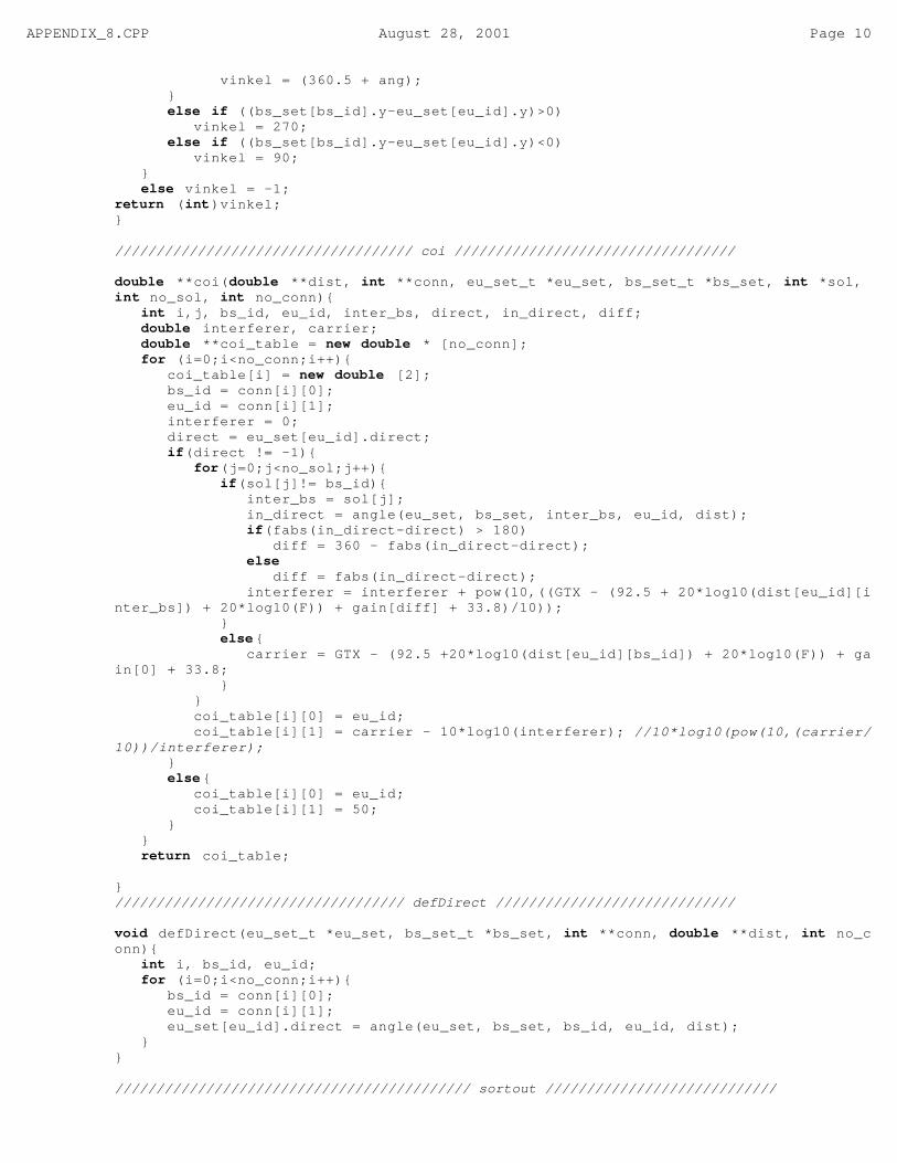
APPENDIX_8.CPP August 28, 2001 Page 10
vinkel = (360.5 + ang); } else if ((bs_set[bs_id].y-eu_set[eu_id].y)>0) vinkel = 270; else if ((bs_set[bs_id].y-eu_set[eu_id].y)<0) vinkel = 90; } else vinkel = -1;return (int)vinkel;}
//////////////////////////////////// coi //////////////////////////////////
double **coi(double **dist, int **conn, eu_set_t *eu_set, bs_set_t *bs_set, int *sol, int no_sol, int no_conn){ int i,j, bs_id, eu_id, inter_bs, direct, in_direct, diff; double interferer, carrier; double **coi_table = new double * [no_conn]; for (i=0;i<no_conn;i++){ coi_table[i] = new double [2]; bs_id = conn[i][0]; eu_id = conn[i][1]; interferer = 0; direct = eu_set[eu_id].direct; if(direct != -1){ for(j=0;j<no_sol;j++){ if(sol[j]!= bs_id){ inter_bs = sol[j]; in_direct = angle(eu_set, bs_set, inter_bs, eu_id, dist); if(fabs(in_direct-direct) > 180) diff = 360 - fabs(in_direct-direct); else diff = fabs(in_direct-direct); interferer = interferer + pow(10,((GTX - (92.5 + 20*log10(dist[eu_id][inter_bs]) + 20*log10(F)) + gain[diff] + 33.8)/10)); } else{ carrier = GTX - (92.5 +20*log10(dist[eu_id][bs_id]) + 20*log10(F)) + gain[0] + 33.8; } } coi_table[i][0] = eu_id; coi_table[i][1] = carrier - 10*log10(interferer); //10*log10(pow(10,(carrier/10))/interferer); } else{ coi_table[i][0] = eu_id; coi_table[i][1] = 50; } } return coi_table;
}/////////////////////////////////// defDirect /////////////////////////////
void defDirect(eu_set_t *eu_set, bs_set_t *bs_set, int **conn, double **dist, int no_conn){ int i, bs_id, eu_id; for (i=0;i<no_conn;i++){ bs_id = conn[i][0]; eu_id = conn[i][1]; eu_set[eu_id].direct = angle(eu_set, bs_set, bs_id, eu_id, dist); }}
/////////////////////////////////////////// sortout ////////////////////////////

APPENDIX_8.CPP August 28, 2001 Page 11
void sortout(int no_conn, double **coi_table){ int i,j,p; double temp[2],min; for (i=0;i<no_conn-1;i++){ min = coi_table[i][1]; p = -1; for(j=i+1;j<no_conn;j++){ if(coi_table[j][1]<min){ min = coi_table[j][1]; p=j; } } if (p != -1){ temp[0]= coi_table[i][0]; temp[1]= coi_table[i][1]; coi_table[i][0] = coi_table[p][0]; coi_table[i][1] = coi_table[p][1]; coi_table[p][0] = temp[0]; coi_table[p][1] = temp[1]; }
}
}
///////////////////////////////////// udskriv ////////////////////////////////void udskrivcoi(int no_conn, double **coi_table){ int i; FILE *fp1; fp1 = fopen(coi_fil, "w"); for(i=0;i<no_conn;i++){ fprintf(fp1, "%8.0f %8f \n", coi_table[i][0], coi_table[i][1]); } fclose(fp1);
}
///////////////////////////////////////////// udskriv /////////////////////////////////
void udskriv(double **dist, bool *usedBS, bool *usedEU, double *final_conn, sortBasestation_t **near_eu, int bs, int eu, struct eu_set_t *eu_set, sortBasestation_t **P_short_end_base, double *load_bs, double **distBB, struct bs_set_t *bs_set, double global_obj, int out_loop){FILE *fp1;fp1 = fopen(connect, "w");
int i,p=0, no_sol, no_conn, count = 0;bool flag = true;double sum_load = 0;double all_load = 0;
find_nearest(P_short_end_base, near_eu, usedBS, eu); sort_end_base(P_short_end_base, eu);
for(i=0;i<bs;i++){ final_conn[i] = 0; load_bs[i] = 0; } for(i=0;i<eu;i++) usedEU[i] = false ;
while (flag){ i=0;

APPENDIX_8.CPP August 28, 2001 Page 12
flag = false ; while (i<eu){ if(legal_conn(P_short_end_base[i], usedBS, distBB, load_bs, final_conn, eu_set, bs, bs_set) && !usedEU[i]){ fprintf(fp1, "%8d %8d %8f\n", P_short_end_base[i]->id+1, P_short_end_base[i]->endId+1, P_short_end_base[i]->dist); usedEU[i] = true; load_bs[P_short_end_base[i]->id] += eu_set[P_short_end_base[i]->endId].demand; final_conn[ P_short_end_base[i]->id] = P_short_end_base[i]->dist; flag = true; } i++; } } fclose(fp1); int *sol = indlaesSOL(&no_sol); // start på evaluering int **conn = indlaesCONN(&no_conn); defDirect(eu_set, bs_set, conn, dist, no_conn); double **coi_table = coi(dist, conn, eu_set, bs_set, sol, no_sol, no_conn); sortout(no_conn, coi_table); for (i=0;i<no_conn;i++){ if (coi_table[i][1]<LIM) count ++; } cout << "Antal end_user med C/I < " << LIM << " " << count << endl; cout << "Andel af end_user med C/I <" << LIM << " " << (double )count/(double )no_conn << endl; udskrivcoi(no_conn, coi_table); // slut på evaluering
for (i=0;i<eu;i++){ all_load += eu_set[i].demand; if(usedEU[i]){ p++; sum_load += eu_set[i].demand; } } FILE *fp4; fp4 = fopen(result, "a"); fprintf(fp4, "****************************************************************************************\n\n\n"); fprintf(fp4, "%-38s %-8d \n","Out_loop", out_loop); fprintf(fp4, "%-38s %-8d \n","Global iteration", GLOBAL_ITER); fprintf(fp4, "%-38s %-8d \n","Lokal iteration", LOCAL_ITER); fprintf(fp4, "%-38s %-8.2f \n","T_start", T_START); fprintf(fp4, "%-38s %-8.2f \n","Cool rate", COOL_RATE); fprintf(fp4, "%-38s %-8.2f \n","Tapering constant", TAPERING_CONST); fprintf(fp4, "%-38s %-8.2f \n","Overlap constant", OVERLAP_CONST); fprintf(fp4, "%-38s %-8d \n","Validate by density", VAL_BY_DENSITY); fprintf(fp4, "%-38s %-8d \n","Validate by demand", VAL_BY_DEMAND); fprintf(fp4, "%-38s %-8d \n","Val. obj by demand", OBJ_BY_DEMAND); fprintf(fp4, "%-38s %-8d \n","Number of base stations", NUMBER_OF_BS); fprintf(fp4, "%-38s %-8d \n","Seed", seed); fprintf(fp4, "%-38s %-8d \n","Number of not connected end_user", (eu-p)); fprintf(fp4, "%-38s %-8.2f \n","Number of End-user hit rate", ((double )p/(double )eu)); fprintf(fp4, "%-38s %-8.2f \n","End-user demand hit rate", (sum_load/all_load)); fprintf(fp4, "%-38s %-8.2f \n","Best objective value", global_obj); fprintf(fp4, "%-30s %d %-4s %-8.2d \n","Number of end_users with C/I <", LIM, " ", count); fprintf(fp4, "%-29s %d %-5s %-8.2f \n","Share of end_users with C/I <", LIM, " ", (double )count/(double )no_conn); fprintf(fp4, "%-38s %-8d \n\n","Total number of not connected end_user", (eu-p)+ count); for(i=0;i<ini;i++) fprintf(fp4, "%-15s %-15d \n","Fixed base station", int_solution[i]);

APPENDIX_8.CPP August 28, 2001 Page 13
fprintf(fp4, "\n %-15s %-15s %-15s","Base station", "Load", "x_coordinate"); fprintf(fp4, "%-15s %-15s \n","y_coordinate", "Radius");
for(i=0;i<bs;i++) if(usedBS[i]){ fprintf(fp4, "%-15d %-15.0f %-15.3f", i, load_bs[i], bs_set[i].x); fprintf(fp4, "%-15.3f %-15.3f \n",bs_set[i].y, final_conn[i]); } fprintf(fp4, "\n\n"); fclose(fp4); delete [] sol; for (i=0;i<no_conn;i++){ delete coi_table[i]; delete conn[i]; } delete [] coi_table; delete [] conn;
}//////////////////////////////////////// new2global ////////////////////////////////////
void new2global(bool *usedBS, bool *global_sol, int bs, double *obj, double *global_obj){ int i; for (i=0;i<bs;i++){ global_sol[i] = usedBS[i];// if(usedBS[i])// cout << i << " "; }// cout << endl; *global_obj = *obj;}
//////////////////////////////////////// new2prev /////////////////////////////////////
void new2prev(double *obj, double *prev_obj){ *prev_obj = *obj;}
///////////////////////////////////// find_new_sol ////////////////////////////////////
void find_new_sol(bool *usedBS, int bs, int *add, int *remove, bool *bin_solution){ double p; p = ran(); if(p<=(1-q_p)){ *add = ((int)(ran()*bs)); while (usedBS[*add]) *add = ((int)(ran()*bs)); usedBS[*add] = true; } else{ *add =-1; cout << "no add " << endl; } if(p>=(q_p/2)){ *remove = ((int)(ran()*bs)); if(RESTART_SOL){ while (!usedBS[*remove]) *remove = ((int)(ran()*bs)); } else{ while ((!usedBS[*remove])||(bin_solution[*remove])) *remove = ((int)(ran()*bs));

APPENDIX_8.CPP August 28, 2001 Page 14
} usedBS[*remove] = false ; } else{ *remove = -1; cout << "no remove " << endl; }}
//////////////////////////////////////// restore_prev /////////////////////////////////
void restore_prev(bool *usedBS, int *add, int *remove, double *obj, double *prev_obj){ if(*add > -1) usedBS[*add] = false ; if(*remove > -1) usedBS[*remove] = true; *obj = *prev_obj;}
///////////////////////////////////////// p_screen ///////////////////////////////////
void p_screen(bool *global_sol, bool *usedEU, double *load_bs, struct bs_set_t *bs_set, int bs, int eu, double *final_conn){ int i, user = 0; cout << setw(5) << "bs" << setw(12) << "load_bs[i]" << setw(12) << "bs_set[i].x" << setw(12) << "bs_set[i].y" << setw(14) << "final_conn[i]" << endl; for (i=0;i<bs;i++) if(global_sol[i]) cout << setw(5) << i << setw(12) << load_bs[i] << setw(12) << bs_set[i].x << setw(12) << bs_set[i].y << setw(12) << final_conn[i] << endl; for (i=0;i<eu;i++) if(!usedEU[i]) user++; cout << setw(10) << user << " ikke forbundende brugere " << endl;}
/////////////////////////////////////////// Main /////////////////////////////////////
int main(){
int i, global_count, local_count, accept, avr =0,t_count = 0, new_seed; int eu,bs, add, remove,out_loop; double obj = 0, global_obj = 1000000, prev_obj = 1000000, temperature; //bool flag; eu = counter(enduser); bs = counter(basestation); bool *usedEU = new bool[eu]; bool *usedBS = new bool[bs]; bool *global_sol = new bool[bs]; bool *bin_solution = new bool[bs]; int *swap = new int[bs]; for (i=0;i<eu;i++){

APPENDIX_8.CPP August 28, 2001 Page 15
usedEU[i] = false ; if(i<bs){ usedBS[i] = false ; global_sol[i] = false ; bin_solution[i] = false ; swap[i] = 0; } } for (i=0;i<ini;i++) bin_solution[int_solution[i]] = true; FILE *fp2;
FILE *fp; double *final_conn = new double [bs]; double *load_bs = new double [bs]; for (i=0;i<bs;i++){ load_bs[i] = 0; final_conn[i] = 0; }
interpolate(); struct eu_set_t *eu_set = indlaesEU(eu); struct bs_set_t *bs_set = indlaesBS(bs); sortBasestation_t **P_short_end_base = new sortBasestation_t *[eu]; double **dist = defDist(eu_set, bs_set, eu, bs); double **distBB = defDistBB(bs_set, bs); sortBasestation_t **near_eu = sortBasestation(bs, eu, dist, bs_set); alter_dist(bs_set, bs); if(VAL_BY_DENSITY) defDensity(eu, eu_set); for(NUMBER_OF_BS = min_bs;NUMBER_OF_BS<=max_bs;NUMBER_OF_BS++){ new_seed = seed; for(out_loop=0;out_loop<out_cnt;out_loop++){ fp = fopen(output, "w"); new_seed += (137*out_loop); srand(new_seed); for (i=0;i<bs;i++) usedBS[i]=false ; new_startsol(usedBS, bs); find_nearest(P_short_end_base, near_eu, usedBS, eu); sort_end_base(P_short_end_base, eu); obj = conn_end(P_short_end_base, eu_set, distBB, final_conn, load_bs, usedBS, usedEU, eu, bs, near_eu, bs_set); new2global(usedBS, global_sol, bs, &obj, &global_obj); new2prev( &obj, &prev_obj); temperature = T_START; local_count = 0; global_count = 0; accept = 0; //flag = true; cout << setw(15) << "global_count" << setw(12) << "accept" << setw(12) << "global_obj" << setw(12) << "obj" << endl; while (global_count < GLOBAL_ITER){ while ( (local_count < LOCAL_ITER)&&(accept < ACCEPTRATE)){ t_count++; find_new_sol(usedBS, bs, &add, &remove, bin_solution);// swap[add] +=1;// swap[remove] +=1; obj = conn_end(P_short_end_base, eu_set, distBB, final_conn, load_bs, usedBS, usedEU, eu, bs, near_eu, bs_set); if(obj <= prev_obj){ new2prev(&obj, &prev_obj); accept++;

APPENDIX_8.CPP August 28, 2001 Page 16
} else if(exp((prev_obj - obj)/temperature) > ran()){ new2prev(&obj, &prev_obj); accept++; } else restore_prev(usedBS, &add, &remove, &obj, &prev_obj);
if(obj < global_obj){ new2global(usedBS, global_sol, bs, &obj, &global_obj); cout << " ***** New global_obj ***** " << global_obj << " at count " << t_count << endl; } local_count++; fprintf(fp, "%10f %10f %10f\n", obj, global_obj, temperature); } global_count++; temperature *= COOL_RATE; avr += accept; local_count = 0; cout << setw(15) << global_count << setw(12) << accept << setw(12) << global_obj << setw(12) << obj << endl; accept = 0; } fclose(fp); cout << "average accept " << (avr/GLOBAL_ITER) << endl; fp2 = fopen(solution, "w"); for (i=0;i<bs;i++) if(global_sol[i]){ fprintf(fp2, "%d\n", (i+1) ); } fclose(fp2); udskriv(dist, global_sol, usedEU, final_conn, near_eu, bs, eu, eu_set, P_short_end_base, load_bs, distBB, bs_set, global_obj,out_loop); p_screen(global_sol, usedEU, load_bs, bs_set, bs, eu, final_conn); t_count = 0; } // end outerloop } //end base station for loop system("pause");}