Simulated annual changes in plant functional types and ... · Simulated annual changes in plant functional types and their ... (TP) exerts strong ... and the partition of net radiation

Biogeosciences, 13, 3533–3548, 2016www.biogeosciences.net/13/3533/2016/doi:10.5194/bg-13-3533-2016© Author(s) 2016. CC Attribution 3.0 License.

Simulated annual changes in plant functional types and theirresponses to climate change on the northern Tibetan PlateauLan Cuo1, Yongxin Zhang2, Shilong Piao1, and Yanhong Gao3

1Center for Excellence in Tibetan Plateau Earth Sciences, Key Laboratory of Tibetan Environment Changes andLand Surface Processes, Institute of Tibetan Plateau Research, Chinese Academy of Sciences, Beijing, China2Research Applications Laboratory, National Center for Atmospheric Research, Boulder, Colorado, USA3Key Laboratory of Land Surface Process and Climate Change in Cold and Arid Regions, Cold and Arid RegionsEnvironmental and Engineering Research Institute, Chinese Academy of Sciences, Lanzhou, China

Correspondence to: Lan Cuo ([email protected])

Received: 16 February 2016 – Published in Biogeosciences Discuss.: 18 February 2016Revised: 27 May 2016 – Accepted: 31 May 2016 – Published: 17 June 2016

Abstract. Changes in plant functional types (PFTs) have im-portant implications for both climate and water resources.Still, little is known about whether and how PFTs havechanged over the past decades on the northern TibetanPlateau (NTP) where several of the top largest rivers in theworld are originated. Also, the relative importance of at-mospheric conditions vs. soil physical conditions in affect-ing PFTs is unknown on the NTP. In this study, we usedthe improved Lund–Potsdam–Jena Dynamic Global Vege-tation Model to investigate PFT changes through examin-ing the changes in foliar projective coverages (FPCs) dur-ing 1957–2009 and their responses to changes in root zonesoil temperature, soil moisture, air temperature, precipitationand CO2 concentrations. The results show spatially hetero-geneous changes in FPCs across the NTP during 1957–2009,with 34 % (13 %) of the region showing increasing (decreas-ing) trends. Dominant drivers responsible for the observedFPC changes vary with regions and vegetation types, butoverall, precipitation is the major factor in determining FPCchanges on the NTP with positive impacts. Soil tempera-ture increase exhibits small but negative impacts on FPCs.Different responses of individual FPCs to regionally varyingclimate change result in spatially heterogeneous patterns ofvegetation changes on the NTP. The implication of the studyis that fresh water resources in one of the world’s largest andmost important headwater basins and the onset and intensityof Asian monsoon circulations could be affected because ofthe changes in FPCs on the NTP.

1 Introduction

Vegetation dynamics can directly affect water, energy andcarbon balances in the coupled land–atmosphere system byresponding and providing feedbacks to climate change (Bo-nan et al., 1992, 2003; Rogers et al., 2013; Ahlstrom et al.,2015; Mengis et al., 2015; Paschalis et al., 2015; Petermanet al., 2015; Sitch et al., 2015; Cuo, 2016). In recent years,dynamic global vegetation models (DGVMs) coupled withatmospheric processes have become valuable tools for exam-ining and understanding the interactive dynamics in carbon,water, and energy exchanges between biosphere and atmo-sphere. The representation of dynamic vegetation has alsobecome a key component in the earth system models sincethe last decade (Levis et al., 2004; Sato et al., 2007; Hopcroftand Valdes, 2015). There are many widely used DGVMsthat include TRIFFID (Cox, 2001), LPJ (Sitch et al., 2003),BIOME-BGC (Tatarinov and Cienciala, 2006), CENTURY(Smithwick et al., 2009), and OCHIDEE (Ciais et al., 2008),just to name a few. Most of these DGVMs employ the so-called climate envelop approach to control the redistributionof plant, whereas TRIFFID uses the Lotka–Volterra repre-sentation of competitive ecological processes for plant redis-tribution (Fisher et al., 2015).

One common way to describe vegetation in many DGVMsis the adoption of the term plant functional type (PFT) forclassifying plants into discrete groups according to their eco-logical, physiological and phylogenetic traits (Cox, 2001;Sitch et al., 2003). In many of the state-of-the-art hydro-

Published by Copernicus Publications on behalf of the European Geosciences Union.

3534 L. Cuo et al.: Simulated annual changes in plant functional types

logical and land surface models, PFT is both an input fordriving the land–atmosphere processes (e.g., Liang et al.,1994, 1996; Wigmosta et al., 1994) and an output of dy-namic vegetation simulations (e.g., Sitch et al., 2003). Whenclimate changes, PFTs may migrate or retreat depending onbioclimatic limits and availability of water and light (Pear-son et al., 2013). For example, Jiang et al. (2012) examinedthe Lund–Potsdam–Jena Dynamic Global Vegetation Model(LPJ-DGVM) simulations and showed that temperate treeswere more sensitive to climate change than boreal trees andperennial C3 grasses, suggesting that anomalous warming inthe northern high latitudes could change the composition ofPFTs and cause the northward migration of temperate trees.Changes in the composition of PFTs due to climate changecould also modify the foliar projective coverage (FPC, theproportion of ground area that is covered by leaves), an im-portant quantity in determining water, energy, and carbon ex-change (Weiss et al., 2014; Meng et al., 2015). Given thefact that evapotranspiration and photosynthesis are closelyrelated to the foliar properties (Swank and Douglass, 1974;Huber and Iroume, 2001; Zhang et al., 2015), some dynamicvegetation models use FPC to represent PFT (e.g., Sitch etal., 2003).

Due to its massive size and high altitude, the TibetanPlateau (TP) exerts strong influence on regional and globalclimate through mechanical and thermal-dynamic forcing(Yanai et al., 1992; Wang et al., 2008). The TP is character-ized by complex terrain, heterogeneous land surfaces, spa-tially varying energy and water patterns, diverse ecosystemsand bioclimatic zones (Yeh and Gao, 1979; CAS, 2001).The surface conditions of the TP, such as snow cover, soilmoisture and vegetation all affect the strength and evolu-tion of the East Asian and South Asian monsoons (Reiterand Gao, 1982; Ye and We, 1998; Zhang et al., 2004; Qiu,2008). It is also the headwater region of the major riversin Asia (Cuo et al., 2014). In particular, the northern TP(NTP; 30–40◦ N, 90–105◦ E) where the Yellow, Yangtze andMekong Rivers originate, is crucially important in provid-ing water and other ecosystem services to the plateau it-self and the downstream regions hosting billions of popu-lation. Changes in the composition of different PFTs, andconsequently FPCs, could substantially affect surface evapo-transpiration, soil water storage and streamflow (Cuo et al.,2009, 2013a, 2015; Weiss et al., 2014; Dahlin et al., 2015),and the partition of net radiation into the sensible and la-tent heat fluxes, consequently affecting the onset and inten-sity of south and east Asian monsoon circulations (Wu et al.,2007; Cui et al., 2015). Although there are some studies thatconnect NDVI (normalized difference vegetation index) andNPP (net primary production) to precipitation, air tempera-ture, and CO2 concentrations on the TP (Zhong et al., 2010;Chen et al., 2012; Piao et al., 2012), very few studies haveexamined PFT changes and their relationships with climatefor the region (Wang et al., 2011).

Besides precipitation, air temperature and CO2 change im-pacts on the plants, changes in soil temperature and soilmoisture could also affect heterotrophic respiration (litter de-composition, soil carbon release, etc.) and vegetation root de-velopment. Jin et al. (2013) found that spatial patterns andtemporal trends of phenology were parallel with the corre-sponding soil physical conditions over the TP, and that 1 ◦Cincrease in soil temperature could advance the start of thegrowing season by 4.6–9.9 days. On the TP where a vast areaof seasonally frozen (SFS) and permafrost (PFS) soil exists(Cheng and Jin, 2013), global warming induced frozen soildegradation (Cuo et al., 2015) could potentially affect litterdecomposition and plant phenology (Jin et al., 2013).

To date, little is still known about the changes in PFTs orFPC on the NTP in recent decades, much less the mecha-nisms behind these changes, largely due to the lack of long-term observation data and appropriate research tools. Thisknowledge gap greatly limits our understanding of TP’s veg-etation dynamics in response to climate change and the asso-ciated implications in the regional and global water, energyand carbon cycles. This study aims to fill this knowledge gapby investigating the changes in PFTs on the NTP in 1957–2009 and the underlying mechanisms using a dynamic vege-tation model, the LPJ-DGVM model. Important atmosphericand soil variables that could significantly affect PFT changes,including precipitation, air temperature, CO2 concentration,soil temperature and soil moisture, are examined and theirimportance is compared using a dynamic vegetation model.

2 Methods and data

2.1 Study area

The NTP lies between 1400 and 6100 m above sea level,with an average elevation of around 3900 m (Fig. 1). Fivelarge mountains, the Hengduan in the southeast, the Tanggulain the southwest, the Kunlun in the center, the Arjin in thenorthwest, and the Qilian in the north are located on the NTP.Vegetation on the NTP changes from forest in the southeastto grassland and desert in the northwest, with major veg-etation types including temperate evergreen needleleaf for-est, summergreen needleleaf and broadleaf forest, temperateshrub/grassland, alpine meadow, alpine steppe, sparsely veg-etated bare land and desert. Annual precipitation ranges from1000 mm in the southeast to less than 100 mm in the north-west. Annual air temperature is high in the low elevation(about 15 ◦C) and low in the high elevation (about −10 ◦C).Details of the spatial patterns of the climate elements andtheir changes on the NTP over the past five decades can befound in Cuo et al. (2013b).

Biogeosciences, 13, 3533–3548, 2016 www.biogeosciences.net/13/3533/2016/

L. Cuo et al.: Simulated annual changes in plant functional types 3535

80˚ 88˚ 96˚ 104˚ 112˚ 120˚ 128˚

24˚

32˚

40˚

48˚

90˚ 92˚ 94˚ 96˚ 98˚ 100˚ 102˚ 104˚30˚

32˚

34˚

36˚

38˚

40˚

Qinghai 1

23

4 56

7

8

9

10

11

12

13

14

1600

2400

3200

4000

4800

5600

6400

Ele

vatio

n (m

)

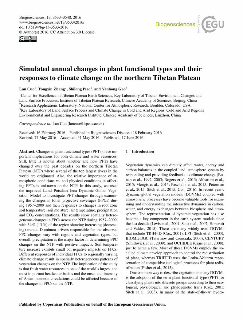
Figure 1. Geographic locations of the study domain and the sta-tions. Black lines outline the boundary of the Qinghai Province.Stars represent the stations whose observations are used to developthe linear regression relationships between daily air temperature and0–40 cm depth daily soil temperature. Stations denoted as diamondsare for monthly soil temperature evaluation and circles are for an-nual soil temperature evaluation. The stations are the following: 1:Mengyuan; 2: Maduo; 3: Wudaoliang; 4: Mangai; 5: Lenghu; 6 Qil-ian; 7: Xinghai; 8: Zaduo; 9: Xidatan; 10: Germud; 11: Amdo; 12:D66; 13: MS3608; 14: Tuotuohe. Among the stations, Wudaoliang,Xidatan, Amdo, D66, MS3608 and Tuotuohe are permafrost soilsites and all others are seasonally frozen soil sites. Stations 1–10and circles were used for soil temperature validation while stations11–14 (empty squares) were used for soil moisture validation.

2.2 The LPJ model and its parameterizations for theNTP

We used the LPJ-DGVM model (Sitch et al., 2003; Gertenet al., 2004; LPJ hereafter) to simulate vegetation dynam-ics, carbon cycle and biogeophysical properties. Vegetationdynamics in LPJ are driven by the processes of competitionfor water, light and nutrients among plant functional types,with different rates of plant carbon assimilation and alloca-tion, reproduction, and survival. LPJ can simulate photosyn-thesis, transpiration, soil organic matter and litter dynamicsand fire disturbance at daily time step, and resource compe-tition, tissue turnover, population dynamics at annual timestep. Plant establishment is determined by bioclimatic lim-its. Probability of plant mortality is controlled by the inter-actions among light competition, low growth efficiency, anegative carbon balance, heat stress and bioclimatic limits.

LPJ couples fast hydrological and physiological processeswith slower ecosystem processes using daily, monthly, andyearly time scales (Bonan et al., 2003), and has been success-fully applied in the simulation of global and regional vege-tation dynamics and large scale PFT distributions (Smith etal., 2001; Sitch et al., 2003, 2005, 2008; Gerten et al., 2004;Murray, 2014; Steinkamp and Hickler, 2015).

Six PFTs, temperate needleleaf evergreen trees, temper-ate broadleaf evergreen trees, temperate broadleaf summer-green trees, perennial alpine meadow grasses, perennialalpine steppe grasses, and perennial temperate summergreenscrub/grassland are compiled and used in the model to repre-sent the major vegetation types on the NTP, based on phys-iognomic (tree or herbaceous), bioclimatic (temperate, bo-real or alpine), phenological (evergreen or summergreen),and photosynthetic (C3 or C4) properties of the plants. Thevegetation state of each of the 0.25◦× 0.25◦ grid cells in LPJis a mixture of PFTs that can be distinguished by their FPCs.FPC of an individual PFT, ranging from 0 (zero coverage)to 100 (full coverage), is a function of crown area (for treesonly), individual PFT density and LAI (leaf area index) , andis calculated by the Lambert–Beer law (Sitch et al., 2003).The total FPC of a given space is the sum of the FPCs of allPFTs in that space.

On the NTP, vegetation root system is concentrated in thetop 0.4 m depth where soil undergoes seasonal freezing andthawing cycles. The accuracy of heat and moisture contentrepresentation in the top 0.4 m soil is therefore vital for mod-elling vegetation dynamics and carbon cycle in this region.In this work, LPJ is configured with two soil layers, 0–0.4 m(top layer) and 0.4–1.0 m (bottom layer) below surface, forbetter accounting for water and energy states of the top soillayer under repeated freezing and thawing cycles on the NTP,while at the same time maintaining its computational effi-ciency for large scale simulations. Daily temperature of thetop soil layer is calculated by linearly regressing it with dailyair temperature. The linear relationship is obtained from fivestations (stars in Fig. 1) where both soil temperature and airtemperature observations are available. These five stationsare located in the different parts of the NTP and representvarious land cover types (temperate shrub/grassland, alpinemeadow, alpine steppe and desert) and soil conditions (SFSand PFS). Depending on the stations, the observation pe-riods are different. Both monthly and annual soil tempera-ture at stations with observation periods greater than 2 yearsare chosen for the validation of simulated soil temperature.The linear regression equations are developed separately fornormal (regular soil moisture) and desert (dry) soils. Fornormal soil, daily soil (0–0.4 m depth), and air tempera-ture are obtained from Mengyuan (1983–2009, SFS), Maduo(1980–2009, SFS) and Wudaoliang (2005–2006, PFS; Eq. 1).For desert dry soils where monthly soil moisture is usuallyaround 0.1 m3 m−3, daily soil, and air temperature are ob-tained from the Mangai (1988–2009) and Lenghu (1980–2009) stations (Eq. 2). Note that desert dry soil temperature

www.biogeosciences.net/13/3533/2016/ Biogeosciences, 13, 3533–3548, 2016


can change quickly due to the lower thermal capacity of dryair (1000 J K−1 kg−1) than that of water (4188 J K−1 kg−1),and the slope for desert dry soil is larger than that for normalsoil. Eqs. (1) and (2) are expressed as follows:

ST1= 0.8753×AT+ 3.1623, θ > 0.1; R2= 0.94 (1)

ST1= 1.0873×AT+ 3.9063, θ ≤ 0.1; R2= 0.97, (2)

where ST1 is daily soil temperature (◦C) in 0–0.4 m depth,AT is daily air temperature(◦C), and θ is total soil moisture(m3 m−3). R2 is coefficient of determination.

Soil temperature in 0.4–1.0 m depth is assumed to be alagged exponential function of the top layer soil temperature.The equations are as follows:

ST2= ST1+ (TA−ST1)× e−T s (3)

TA= a+ b×(Nd− 1− T s×

3652π

)(4)

T s =D2×

34√

Qd× 86400×365/π(5)

Qd =KCs, (6)

where K and Cs are heat conductivity (W m−1 K−1) and vol-umetric heat capacity (J m−3 K−1), respectively, that are cal-culated based on the soil mineral and organic content andmoisture conditions and are updated at a daily time step; Qdis heat diffusivity (m2 s−1); D2 is the depth of the secondlayer; Nd is the number of days in a year; a and b are thelinear regression coefficients of daily air temperature and thenumbers of days in a month, respectively, and are updatedat a monthly time step. Equation (4) calculates the lag ofthe thermal change in the second layer soil temperature. Theequations employed for the second layer soil temperature arethe modified version of the originals used in LPJ.

Total soil moisture in the top soil layer is obtained from thebalance between precipitation input, soil evapotranspirationand percolation. Ice and liquid content is calculated basedon soil temperature. If soil temperature is below 0 ◦C, soilliquid content is calculated by using freezing point depres-sion equation. Ice content is the difference between total soilmoisture and liquid water content. When soil temperature isgreater than 0 ◦C, soil moisture is liquid and ice content iszero. The equations are the following:

θl = ϕ×

(−Lf×ST1

273.16× g× bp

)− 2.0n−3

ST1< 0 θi = θ − θl ST1< 0 (7)

where θ is total soil moisture and subscripts l and i representliquid and ice, respectively; φ is soil porosity; Lf is latentheat of fusion (3.337× 105 J kg−1); g is gravitational accel-eration (9.81 m s−2); bp is the bubbling pressure (m); and n

is the exponent in Campbell’s equation for hydraulic conduc-tivity. The second layer soil moisture is calculated using thesimilar equations, and it is the aggregation of liquid and icecontent, runoff, percolated moisture from the top layer andto the baseflow. Runoff is generated when liquid soil contentis greater than porosity, and percolation is generated whenliquid soil content is greater than soil water holding capacity.Runoff and baseflow are produced in both soil layers and areremoved from soil moisture. Soil moisture observations arerare on the NTP. Only 1-year observations at four permafrostsites are available during the study period (see Fig. 1) andthey are used for soil moisture validation.

The implementation of the aforementioned processes inthe LPJ model requires seven additional soil parameters foreach of the two soil layers: Campbell’s exponent n, bubblingpressure bp, bulk densities for organic matter and soil min-eral, particle densities for organic matter and soil mineral,and quartz content. Soil porosity φ is calculated from soilbulk density and soil particle density. These parameters areoften used in surface hydrological models for calculating soilhydrological properties (e.g. Liang et al., 1994, 1996; Wig-mosta et al., 1994), and are provided for various soil texturetypes in the LPJ model. These additional parameters togetherwith the original parameters for soil texture, soil percolationrates and water holding capacity constitute the new soil pa-rameter sets. These modifications eliminate the use of fixedheat diffusivity at 0, 15 and 100 % water content in the orig-inal model version, instead here the diffusivity varies withthermal conductivity and capacity as shown in Eq. (6).

2.3 Forcing data and observations

Forcing data used in the LPJ model include monthly air tem-perature, precipitation, wet days, cloud cover amount and an-nual CO2 concentrations. Monthly air temperature, precipita-tion and wet days, all at 0.25◦× 0.25◦ resolution, were fromCuo et al. (2013b). Cloud cover data came from the ClimateResearch Unit of the University of East Anglia (Mitchell andJones, 2005) at 0.5◦× 0.5◦ resolution and were regriddedto 0.25◦× 0.25◦ resolution assuming uniform distribution ofcloud cover within each 0.5◦× 0.5◦ grid cell. Annual CO2concentrations were obtained from the Mauna Loa Observa-tory operated by National Oceanic and Atmospheric Admin-istration (NOAA). Missing CO2 observations for 1957–1958were filled in by extrapolating the regression between annualCO2 concentrations and the corresponding years. Soil tex-ture data were from the Harmonized World Soil Data v1.0(FAO, 2008). Elevation data were from the Shuttle RadarTopography Mission (SRTM) and were interpolated to the0.25◦× 0.25◦ grids using cubic convolution.

2.4 Analysis methods

To spin up, the LPJ model was run iteratively for 1000 yearsusing the 1957–1986 climate data and starting from bare



Table 1. Calibrated parameters of plant functional types in the Lund–Potsdam–Jena DGVM model.

Plant functional types gmin GDDs GDD5 min Int Ws-m RD0 TLCO2 TUCO2 TLP TUP TLcold(mm s−1) (◦C) (◦C) (◦C) (◦C) (◦C)

Temperate broadleaf evergreen trees (TBLE) 1.6 400 900 2.5 0.2 0.8 −3 30 15 30 −0.1Temperate needleleaf evergreen trees (TNEG) 1.8 300 600 2.7 0.4 0.8 −10 15 5 20 −15.5Temperate broadleaf summergreen trees (TBSG) 1.5 300 700 1.0 0.2 0.8 −3 20 5 20 −10Perennial alpine meadow (PAMD) 0.05 70 60 0.1 0.2 1.0 −6 15 0 15 −20Perennial alpine steppe (PASP) 0.05 10 20 0.1 0.2 1.0 −20 5 −7 5 −25Temperate summergreen scrub/grassland (TSGS) 0.4 200 500 0.5 0.2 1.0 −10 18 5 18 −10

Note: gmin: minimum canopy conductance; GDDs: number of growing degree days to attain full leaf cover; GDD5 min: 5 ◦C based minimum degree day; Int: interception storage; Ws-m: water scalar value atwhich leaves shed by drought for deciduous plant; RD0: fraction of roots in the upper soil layer (0–40 cm); TLCO2: lower temperature limit for CO2 absorption; TUCO2: upper temperature limit for CO2absorption; TLP: lower temperature limit for photosynthesis; TUP: upper temperature limit for photosynthesis; TLcold: lower limit of the coldest monthly mean temperature.

Table 2. Scenarios used for examining the FPC sensitivity to cli-mate elements.

Scenarios Variables changed Changed amount

S1 40 cm-deep daily soil temperature (ST1) +1 ◦CS2 40 cm-deep daily soil moisture (SM1) +10 %S3 Monthly air temperature (AT) +1 ◦CS4 Monthly precipitation (PRCP) +10 %S5 Annual CO2 +10 %S6 AT, PRCP, wet day, CO2 Trends removedHistorical – –

ground, a common practice among LPJ users. The purposeof this long run is to establish ecosystem equilibrium equiva-lent to the 1957 conditions. Like earlier studies (e.g., Sitch etal., 2003), we assume that after the 1000-year spin-up, vege-tation dynamics, carbon pools, soil thermal and water condi-tions reach the needed equilibrium.

Given the importance of the top 0.4 m soils for vegetationroot system on the NTP, we validate model simulated soiltemperature and moisture in this layer against available ob-servations. Deep layer soil temperature and moisture are alsoevaluated but will not be shown. Mean, correlation coeffi-cient (R) and root mean square error (RMSE) of monthlyand annual mean soil temperature, as well as monthly soilmoisture are examined. FPCs are used to represent vegeta-tion states and PFTs. The spatial patterns of the simulatedFPCs of dominant PFTs are compared with those of the sur-vey maps compiled by CAS (2001), Zheng et al. (2008) andthe MODIS Terra growing season (May–September) aver-aged annual LAI in 2000–2009. Parameters representing thephysiological, phenological and bioclimatic attributes of thesix PFTs are adjusted accordingly to obtain a reasonablematch between the simulated pattern and the survey maps.Soil parameters used are from Cuo et al. (2013a) and modeldefault settings. The calibrated PFT parameters are listed inTable 1.

Following model evaluation, we examine the changes intotal FPCs and FPCs of individual PFTs during 1957–2009in response to climate change. Climate change is representedby changes in air and 40 cm-deep soil temperatures, 40 cm-deep soil moisture, precipitation and atmospheric CO2 con-centration. The Mann–Kendall trend analysis is employed to

investigate the FPC trends. Also, the differences between his-torical simulation and climate trends removed simulation areexamined to identify the changes in FPCs during the past fivedecades.

To investigate the sensitivity of FPCs in each grid cell tochanges in soil temperature and moisture, air temperature,precipitation and CO2, six scenarios (S1–S6) are designed(Table 2). In the baseline scenario (S6), the trends in air tem-perature, precipitation, wet day and CO2 are removed. Soiltemperature and moisture respond to atmospheric forcingsand they are assumed to have no trends when the trends ofatmospheric forcings are removed. The only difference be-tween S1–5 and S6 scenarios is the introduced change in onevariable while keeping the other variables unchanged. Cloudcover remains the same for all scenarios. For precipitation,only the amount but not the frequency is changed. These sce-narios bear similarity to what has been identified over theNTP in recent decades in general in that S1 plus S2, S3, S4and S5 represent regional frozen soil degradation, warming,wetting and elevated CO2 trends, respectively, although therates of changes and spatial patterns differ (Cuo et al., 2013b,2015). Uniform perturbations are introduced to provide thebenchmark for the climate sensitivity comparison across theregion and to derive sensitivity spatial pattern. It is expectedthat the comparisons between the paired S1–S6, S2–S6, S3–S6, S4–S6 and S5–S6 scenarios would reveal the responsesof FPC to the changes in soil temperature, soil moisture, airtemperature, precipitation and CO2, respectively.

Using S1–6 scenarios, we examine elasticity (E), a non-parametric, robust and unbiased estimator (Sankarasubrama-nian et al., 2001; Elsner et al., 2010) that can better measureshow responsive a variable is to a changing condition, in or-der to quantify the degree of the FPC sensitivity to climatechange. Elasticity is calculated as the median of the ratios ofpercentage changes in annual FPC to the percentage changesin an annual climate variable. Positive (negative) E indicatesthat FPC increases (decreases) with changing climate vari-able. Larger E corresponds to higher sensitivity, and when Eis zero FPC is not responding to climate change. In the fol-lowing, we will use EST1, ESM1, EAT, EPRCP and ECO2 todenote the sensitivity of FPCs to the changes in the top layer



−10

0

10

20

Soil

tem

pera

ture

(o C)

2005 2006

Wudaoliang

−10

0

10

20

Soil

tem

pera

ture

(o C)

2004 2005 2006 2007 2008 2009

Maduo

−100

102030

Soil

tem

pera

ture

(o C)

2004 2005 2006 2007 2008 2009

Mengyuan

−100

102030

Soil te

mpe

ratu

re (o C

)

2004 2005 2006 2007 2008 2009

Mangai

−100

102030

Soil te

mpe

ratu

re (o C

)

2004 2005 2006 2007 2008 2009

Lenghu

Obs. Sim.

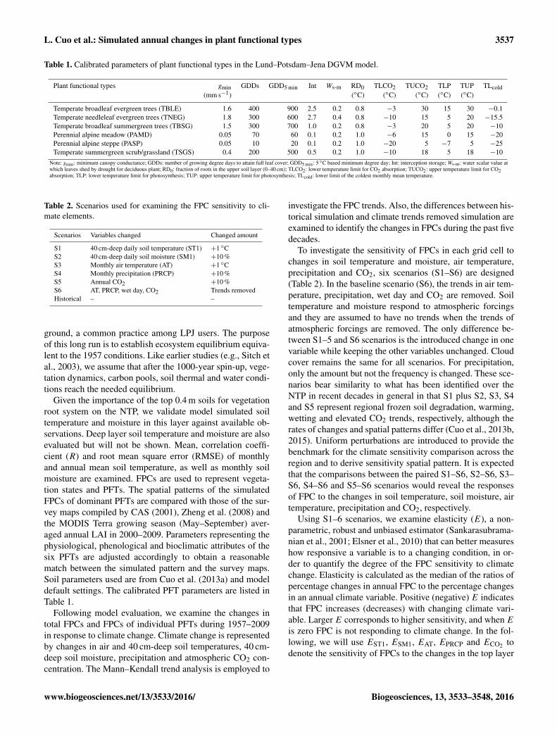
Figure 2. Simulated and observed monthly soil temperature at 5calibration sites.

soil temperature (ST1) and soil moisture (SM1), air temper-ature (AT), precipitation (PRCP), and CO2, respectively.

3 Results

3.1 Evaluations of simulated soil temperature,moisture and FPC

Figure 2 shows the simulated and observed monthly soil tem-perature in the top 0.4 m depth at Wudaoliang (PFS), Maduo(SFS), Mengyuan (SFS), Mangai (SFS, dry desert soil) andLenghu (SFS, dry desert soil). The observations at thesesites are also used to derive the linear regression equationsthat are then applied over the entire domain. At Maduo andMengyuan, the simulated soil temperature matches the ob-served rather well in both magnitude and seasonal cycles.At Wudaoliang, the highest station, the simulated magnitudeof the seasonal cycle in soil temperature is larger than theobserved while the opposite is true at Mangai and Lenghu,two dry desert soil stations. Correlation between the simu-lations and observations is high (R ≥ 0.96) across these fivestations and RMSE ranges from 1.40 ◦C at Maduo to 3.07 ◦Cat Lenghu (Table 3).

−10

0

10

20

Soil

tem

pera

ture

(o C)

2005 2006

Xidatan

−10

0

10

20

Soil

tem

pera

ture

(o C)

2004 2005 2006 2007 2008 2009

Xinghai

−10

0

10

20

Soil

tem

pera

ture

(o C)

2004 2005 2006 2007 2008 2009

Zaduo

−10

0

10

20

Soil

tem

pera

ture

(o C)

2004 2005 2006 2007 2008 2009

Qilian

−10

0

10

20

30

Soil

tem

pera

ture

(o C)

2004 2005 2006 2007 2008 2009

Golmud

Obs. Sim.

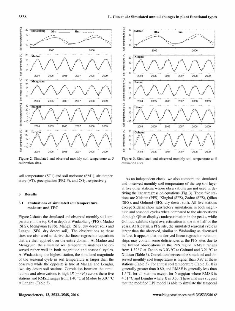
Figure 3. Simulated and observed monthly soil temperature at 5evaluation sites.

As an independent check, we also compare the simulatedand observed monthly soil temperature of the top soil layerat five other stations whose observations are not used in de-riving the linear regression equations (Fig. 3). These five sta-tions are Xidatan (PFS), Xinghai (SFS), Zaduo (SFS), Qilian(SFS), and Golmud (SFS, dry desert soil). All five stationsexcept Xidatan show satisfactory simulations in both magni-tude and seasonal cycles when compared to the observationsalthough Qilian displays underestimation in the peaks, whileGolmud exhibits slight overestimation in the first half of theyears. At Xidatan, a PFS site, the simulated seasonal cycle islarger than the observed, similar to Wudaoling as discussedbefore. It appears that the derived linear regression relation-ships may contain some deficiencies at the PFS sites due tothe limited observations in the PFS region. RMSE rangesfrom 1.32 ◦C at Zaduo to 3.03 ◦C at Golmud and 3.21 ◦C atXidatan (Table 3). Correlation between the simulated and ob-served monthly soil temperature is higher than 0.97 at thesestations (Table 3). For annual soil temperature (Table 3), R isgenerally greater than 0.80, and RMSE is generally less than1.5 ◦C for all stations except for Nangqian where RMSE is4.51 ◦C and Lenghu where R is 0.53. These analyses suggestthat the modified LPJ model is able to simulate the temporal



Table 3. Statistics of the observed and simulated monthly and annual mean soil temperature in 0–40 cm depth. The observations end in 2009for all stations except for Wudaoliang and Xidatan for which the observations end in 2006. R: correlation coefficient; RMSE: root meansquare error.

Stations Start Latitude Longitude Elevation (m) Obs. (◦C) Sim. (◦C) R RMSE (◦C)

Monthly

Wudaoliang 2005 35.217 93.083 4612.2 −1.74 −1.57 0.96 2.89Maduo 2004 34.917 98.217 4272.3 2.13 0.91 0.99 1.40Mengyuan 2004 37.383 101.617 2938.0 5.29 6.05 0.99 1.67Mangai 2004 38.250 90.850 2944.8 8.81 9.70 1.00 2.68Lenghu 2004 38.750 93.333 2770.0 7.50 6.99 1.00 3.07Xinghai 2004 35.583 99.983 3323.2 5.71 5.27 0.99 1.40Zaduo 2004 32.900 95.300 4066.4 5.67 5.31 0.99 1.32Qilian 2004 38.183 100.250 2787.4 5.88 4.70 1.00 2.08Xidatan 2005 35.717 94.133 4538.0 −0.45 −0.70 0.98 3.21Golmud 2004 36.417 94.900 2807.6 9.16 11.89 0.99 3.03

Annual

Mangai 1989 38.250 90.850 2944.8 8.17 8.15 0.82 0.53Lenghu 1981 38.750 93.333 2770.0 7.56 7.82 0.53 0.70Delingha 1982 37.367 97.367 2981.5 7.23 7.85 0.94 0.67Gangcha 1981 37.333 100.133 3345.0 3.59 3.89 0.90 0.38Mengyuan 1984 37.383 101.617 2938.0 4.69 5.63 0.93 0.97Germud 1977 36.417 94.900 2807.6 8.53 10.48 0.68 2.08Qiabuqia 1983 36.267 100.617 2835.0 7.89 8.23 0.82 0.67Xining 1962 36.717 101.750 2295.2 9.02 9.73 0.67 0.90Minhe 1994 36.317 102.850 1813.9 11.22 11.57 0.61 0.74Xinghai 1993 35.583 99.983 3323.2 5.48 5.23 0.80 0.36Qumalai 1984 34.133 95.783 4175.0 3.05 1.46 0.90 1.63Maduo 1981 34.917 98.217 4272.3 1.47 0.88 0.87 0.75Dari 1981 33.750 99.650 3967.5 3.03 2.20 0.87 0.90Henan 1982 34.733 101.600 3670.0 3.85 3.83 0.90 0.79Jiuzhi 1979 33.433 101.483 3628.5 4.58 3.84 0.90 0.79Nangqian 1994 32.200 96.483 3643.7 8.63 4.13 0.92 4.51

evolution of the observed top-layer soil temperature on theNTP with reasonable accuracy.

For monthly soil moisture, the simulations are largely con-sistent with the observations in terms of magnitude and sea-sonal cycles as reflected by RMSE and R in the range of0.08–0.14 m3 m−3 and 0.71–0.83, respectively, based on lim-ited observations (Table 4). Slight overestimation of monthlysoil moisture is noted at D66 and MS3608 (Table 4).

It is difficult to use the Kappa statistics to evaluate thePFT simulation due to the fact that the vegetation classifica-tion systems are different between the observed data sets andthe model simulations and any statistical computation wouldbe subject to large uncertainties. Specifically, the land coverclassification in Zheng et al. (2008) and CAS (2001) are inpolygon format and each polygon contains mixed vegetationclasses without any information of the exact location of eachindividual class within the polygon, which renders it impos-sible to convert from the polygons that represent the mixedvegetation classes as a whole to the model grid cells that rep-resent the mixed individual vegetation classes. For example,

in Zheng et al. (2008), the mixed vegetation class in a poly-gon includes both temperate semi-arid coniferous forest andsteppe in the northeast of the Tibetan Plateau (HIIC1) with-out showing the exact location of the individual vegetationtype; whereas the LPJ simulations are more specific aboutthe location of each vegetation type by using grid cells. Wenevertheless presented as many quantitative comparisons aspossible.

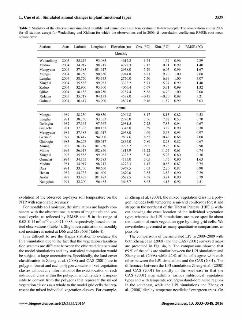
The comparisons of the simulated LPJ in 2000–2009 withboth Zheng et al. (2008) and the CAS (2001) surveyed mapsare presented in Fig. 4a, b. The comparisons showed that69 % of the cells are similar between the LPJ simulation andZheng et al. (2008) while 42 % of the cells agree with eachother between the LPJ simulations and the CAS (2001). Thedifferences between the LPJ simulations Zheng et al. (2008)and CAS (2001) lie mostly in the southeast in that theCAS (2001) map exhibits various subtropical vegetationtypes and with temperate scrub/grassland-dominated regionsin the southeast, while the LPJ simulations and Zheng etal. (2008) display temperate needleleaf evergreen trees. On



Table 4. Statistics of the first layer (0–40 cm) monthly soil moisture. The observation period is August 1997–September 1998.

Stations Latitude Longitude Elev. Mean Obs. Mean Sim. R RMSE(m) (m3 m−3) (m3 m−3) (m3 m−3)

Amdo 32.25 91.63 4700 0.14 0.15 0.76 0.10D66 35.52 93.78 4600 0.08 0.13 0.83 0.10MS3608 31.24 91.78 4610 0.16 0.20 0.80 0.14Tuotuohe 34.22 92.43 4353 0.12 0.13 0.71 0.08

the other hand, the LPJ simulation and the CAS (2001) mapshow more similarity in the northeast where alpine meadowand temperate scrub/grassland are widely distributed than be-tween the LPJ simulations and Zheng et al. (2008).

The annual MODIS Terra LAI obtained from May-September (growing season) MODIS Terra LAI was com-pared with the LPJ simulated FPC for 2000–2009 (Fig. 4c,d). The spatial patterns of the MODIS LAI and the LPJ sim-ulated FPC show similarities to some extent. For example,in the northwest, where LAI is low, FPC is also small. Ma-jor differences exist mainly in the southwest where FPC isgreater than 90 % but LAI is less than 0.3, most likely be-cause of the small leaf area coverage but high density of in-dividual PFTs in the steppe and meadow-dominated regions.

The spatial patterns of the LPJ simulated PFT (Fig. 4a)and the MODIS LAI (Fig. 4c) match quite well in general, inthat barren/sparse grassland corresponds with LAI less than0.2; alpine steppe corresponds with LAI in 0.2–03; alpinemeadow corresponds with LAI in 0.3–0.5; and temperate for-est and scrub/grassland corresponds with LAI greater than0.8. These analyses indicate that the LPJ simulations, thoughnot perfect, are reasonable. Overall, temperate needleleaf ev-ergreen forest (TNEG hereafter), perennial alpine meadow(PAMD), perennial alpine steppe (PASP), perennial temper-ate summergreen shrub/grassland (TSGS), and barren/sparsegrassland prevail over the NTP (Fig. 4a).

3.2 Changes in FPCs and climatic factors

The Mann–Kendall trends of annual total FPC (the sum ofFPCs of all PFTs in one grid cell), top layer annual soil mois-ture and temperature, annual precipitation and air tempera-ture during 1957–2009 are presented in Fig. 5. For FPC, 34 %(13 %) of the region shows increasing (decreasing) trends.Decreasing FPCs are found mostly in the northwest (bar-ren/sparse grassland) and east (TSGS) of the NTP, while in-creasing FPCs are located mainly in the northeast and south-west where alpine meadow, steppe and temperate summer-green shrub/grassland dominate. The variation in the changewas also found by Zhong et al. (2010) who reported that 50 %of the entire TP had increased NDVI with 30 % of the regionhad decreased NDVI during 1998–2006, with most of the in-creases occurring in the alpine steppe and alpine meadow inthe TP. Further, the LPJ simulated Mann–Kendall trends ofNPP (not shown) exhibit similar spatial patterns to those in

30

32

34

36

38

40

90 92 94 96 98 100 102 104

PFT−LPJ

HIIEHIIC1

HIID1

HIID2

HIC1

HIB1

HIIA/B130

32

34

36

38

40

90 92 94 96 98 100 102 104

PFT−CAS

HIIEHIIC1

HIID1

HIID2

HIC1

HIB1

HIIA/B1

Temperate needleleaf evergreen tree

Temperate broadleaf evergreen tree

Temperate broadleaf summergreen tree

Perennial alpine meadow

Perennial alpine steppe

Perennial temperate scrub/grassland

Barren/sparse grassland

Subtropical needleaf tree

Subtropical mixed tree

Subtropical broadleaf summergreen tree

Subtropical broadleaf evergreen tree

Subtropical scrub

Apline marsh

Crop

Water

30

32

34

36

38

40

90 92 94 96 98 100 102 104

HIIEHIIC1

HIID1

HIID2

HIC1

HIB1

HIIA/B1

0.0 0.3 0.6 0.9 1.2 1.5 1.8

MODIS LAI

30

32

34

36

38

40

90 92 94 96 98 100 102 104

HIIEHIIC1

HIID1

HIID2

HIC1

HIB1

HIIA/B1

0 20 40 60 80 100

LPJ FPC (%)

(a) (b)

(c) (d)

Figure 4. Eco-geographic regions from Zheng et al. (2008) (bluelines in a, b, d and red lines in c) and the LPJ simulated dominantplant functional types represented by foliar projective covers (FPCs)under full leaf during 1957–2009 (a); Zheng et al. (2008) andCAS (2001) surveyed maps (b); MODIS Terra LAI and Zheng etal. (2008) maps (c); and LPJ simulated FPC and Zheng et al. (2008)maps (d). The eco-geographic regions are the following: HIIC1:plateau temperate semi-arid high mountain and basin coniferousforest and steppe region; HIID1: plateau temperate arid desert re-gion; HIID2: plateau temperate high mountain arid desert region;HIC1: plateau sub-cold semi-arid alpine meadow-steppe region;HIB1: plateau sub-cold sub-humid alpine shrub–meadow region;HIIA/B1: plateau temperate humid/sub-humid high mountain anddeep valley coniferous forest region; and HIIE: temperate shrubgrass-desert region. Black line outlines the Qinghai Province.

Piao et al. (2012) in that the increase trends prevail in thenortheast and the south of the NTP and more widely spreadthan those of the total FPC. These similarities further demon-



30

32

34

36

38

40

90 93 96 99 102 105

FPC

−2

−1

0

1

2

Tre

nds

(% y

ear−

1 )

30

32

34

36

38

40

90 93 96 99 102 105

PRCP

−4 −2 0 2 4

Trends (mm year−1)

30

32

34

36

38

40

90 93 96 99 102 105

AT

−0.10 −0.05 0.00 0.05 0.10

Trends (oC year−1)

30

32

34

36

38

40

90 93 96 99 102 105

ST1

−0.10 −0.05 0.00 0.05 0.10

Trends (oC year−1)

30

32

34

36

38

40

90 93 96 99 102 105

SM1

−0.006 0.000 0.006

Trends (m3m−3 year−1)

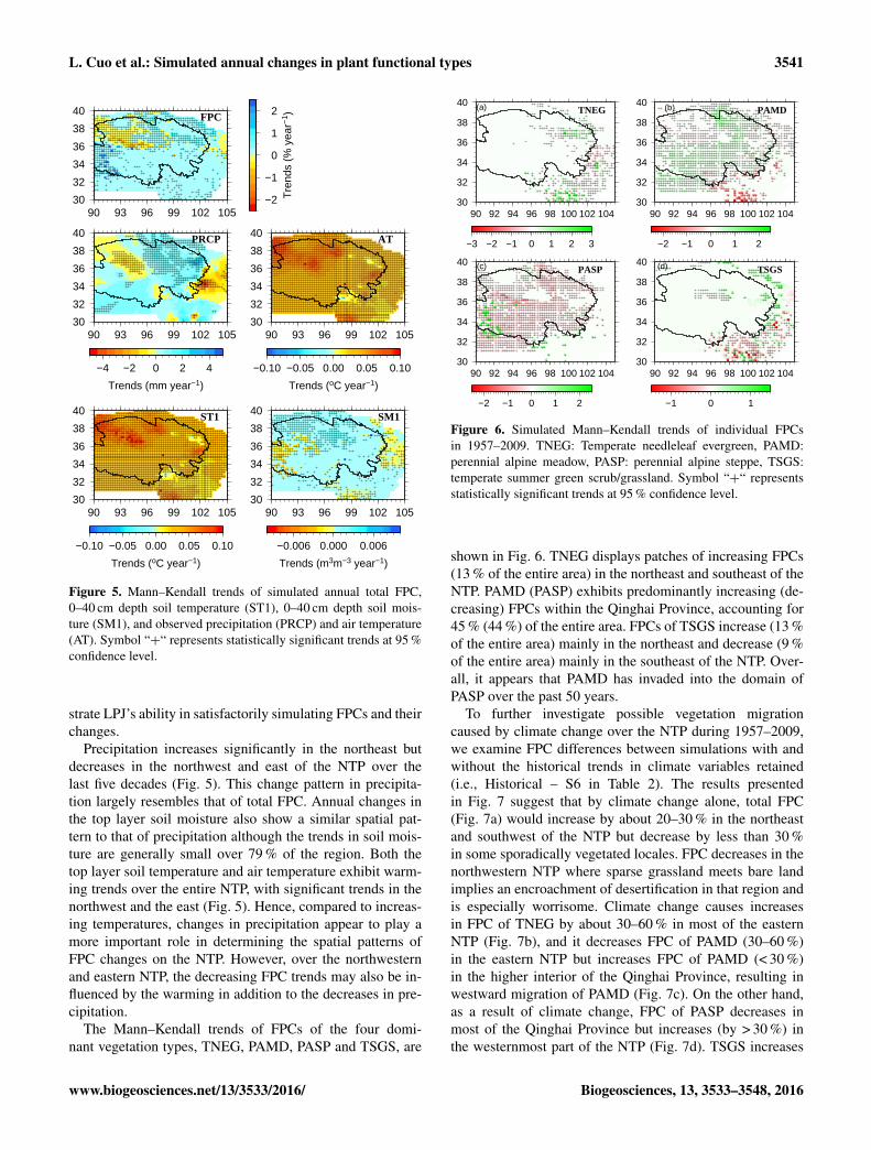
Figure 5. Mann–Kendall trends of simulated annual total FPC,0–40 cm depth soil temperature (ST1), 0–40 cm depth soil mois-ture (SM1), and observed precipitation (PRCP) and air temperature(AT). Symbol “+“ represents statistically significant trends at 95 %confidence level.

strate LPJ’s ability in satisfactorily simulating FPCs and theirchanges.

Precipitation increases significantly in the northeast butdecreases in the northwest and east of the NTP over thelast five decades (Fig. 5). This change pattern in precipita-tion largely resembles that of total FPC. Annual changes inthe top layer soil moisture also show a similar spatial pat-tern to that of precipitation although the trends in soil mois-ture are generally small over 79 % of the region. Both thetop layer soil temperature and air temperature exhibit warm-ing trends over the entire NTP, with significant trends in thenorthwest and the east (Fig. 5). Hence, compared to increas-ing temperatures, changes in precipitation appear to play amore important role in determining the spatial patterns ofFPC changes on the NTP. However, over the northwesternand eastern NTP, the decreasing FPC trends may also be in-fluenced by the warming in addition to the decreases in pre-cipitation.

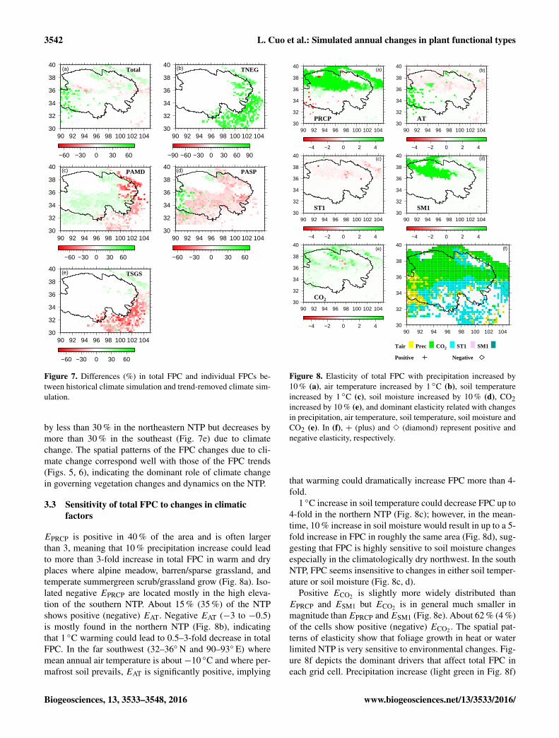
The Mann–Kendall trends of FPCs of the four domi-nant vegetation types, TNEG, PAMD, PASP and TSGS, are

30

32

34

36

38

40

90 92 94 96 98 100 102 104

TNEG

−3 −2 −1 0 1 2 3

30

32

34

36

38

40

90 92 94 96 98 100 102 104

PAMD

−2 −1 0 1 2

30

32

34

36

38

40

90 92 94 96 98 100 102 104

PASP

−2 −1 0 1 2

30

32

34

36

38

40

90 92 94 96 98 100 102 104

TSGS

−1 0 1

(a) (b)

(c) (d)

Figure 6. Simulated Mann–Kendall trends of individual FPCsin 1957–2009. TNEG: Temperate needleleaf evergreen, PAMD:perennial alpine meadow, PASP: perennial alpine steppe, TSGS:temperate summer green scrub/grassland. Symbol “+“ representsstatistically significant trends at 95 % confidence level.

shown in Fig. 6. TNEG displays patches of increasing FPCs(13 % of the entire area) in the northeast and southeast of theNTP. PAMD (PASP) exhibits predominantly increasing (de-creasing) FPCs within the Qinghai Province, accounting for45 % (44 %) of the entire area. FPCs of TSGS increase (13 %of the entire area) mainly in the northeast and decrease (9 %of the entire area) mainly in the southeast of the NTP. Over-all, it appears that PAMD has invaded into the domain ofPASP over the past 50 years.

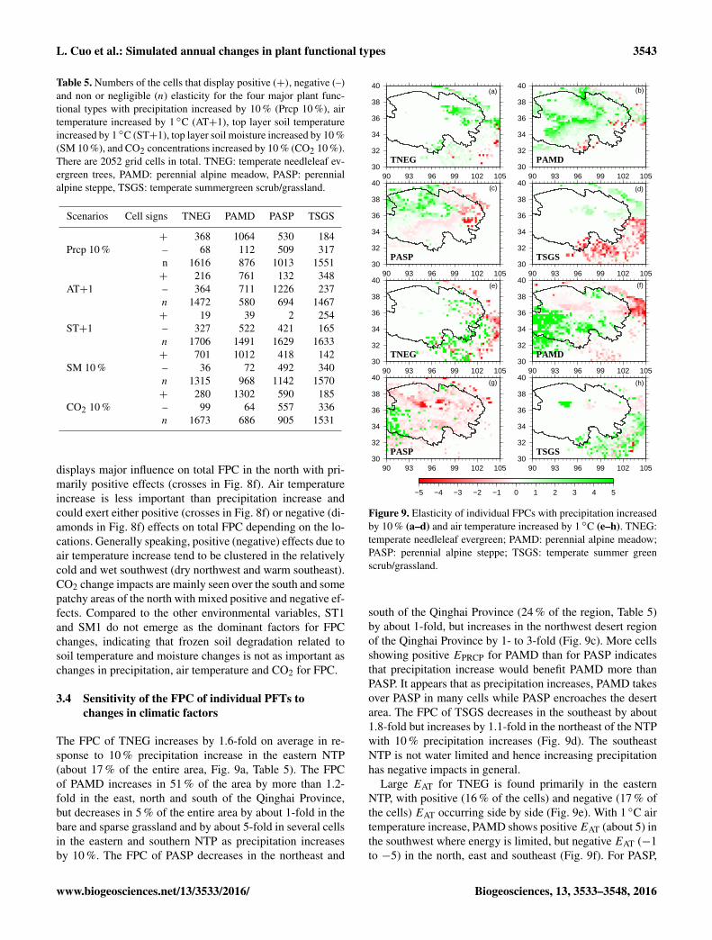
To further investigate possible vegetation migrationcaused by climate change over the NTP during 1957–2009,we examine FPC differences between simulations with andwithout the historical trends in climate variables retained(i.e., Historical – S6 in Table 2). The results presentedin Fig. 7 suggest that by climate change alone, total FPC(Fig. 7a) would increase by about 20–30 % in the northeastand southwest of the NTP but decrease by less than 30 %in some sporadically vegetated locales. FPC decreases in thenorthwestern NTP where sparse grassland meets bare landimplies an encroachment of desertification in that region andis especially worrisome. Climate change causes increasesin FPC of TNEG by about 30–60 % in most of the easternNTP (Fig. 7b), and it decreases FPC of PAMD (30–60 %)in the eastern NTP but increases FPC of PAMD (< 30 %)in the higher interior of the Qinghai Province, resulting inwestward migration of PAMD (Fig. 7c). On the other hand,as a result of climate change, FPC of PASP decreases inmost of the Qinghai Province but increases (by > 30 %) inthe westernmost part of the NTP (Fig. 7d). TSGS increases



30

32

34

36

38

40

90 92 94 96 98 100 102 104

Total

−60 −30 0 30 60

30

32

34

36

38

40

90 92 94 96 98 100 102 104

TNEG

−90 −60 −30 0 30 60 90

30

32

34

36

38

40

90 92 94 96 98 100 102 104

PAMD

−60 −30 0 30 60

30

32

34

36

38

40

90 92 94 96 98 100 102 104

PASP

−60 −30 0 30 60

30

32

34

36

38

40

90 92 94 96 98 100 102 104

TSGS

−60 −30 0 30 60

(a) (b)

(c) (d)

(e)

Figure 7. Differences (%) in total FPC and individual FPCs be-tween historical climate simulation and trend-removed climate sim-ulation.

by less than 30 % in the northeastern NTP but decreases bymore than 30 % in the southeast (Fig. 7e) due to climatechange. The spatial patterns of the FPC changes due to cli-mate change correspond well with those of the FPC trends(Figs. 5, 6), indicating the dominant role of climate changein governing vegetation changes and dynamics on the NTP.

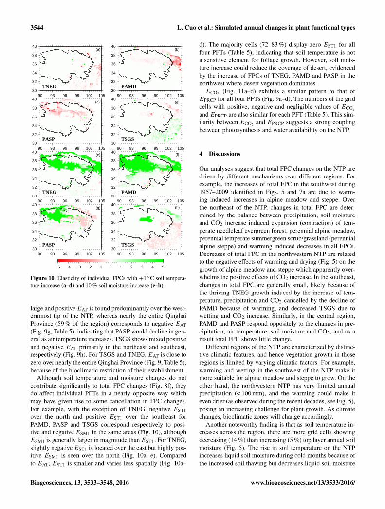
3.3 Sensitivity of total FPC to changes in climaticfactors

EPRCP is positive in 40 % of the area and is often largerthan 3, meaning that 10 % precipitation increase could leadto more than 3-fold increase in total FPC in warm and dryplaces where alpine meadow, barren/sparse grassland, andtemperate summergreen scrub/grassland grow (Fig. 8a). Iso-lated negative EPRCP are located mostly in the high eleva-tion of the southern NTP. About 15 % (35 %) of the NTPshows positive (negative) EAT. Negative EAT (−3 to −0.5)is mostly found in the northern NTP (Fig. 8b), indicatingthat 1 ◦C warming could lead to 0.5–3-fold decrease in totalFPC. In the far southwest (32–36◦ N and 90–93◦ E) wheremean annual air temperature is about −10 ◦C and where per-mafrost soil prevails, EAT is significantly positive, implying

30

32

34

36

38

40

90 92 94 96 98 100 102 104

PRCP

−4 −2 0 2 4

30

32

34

36

38

40

90 92 94 96 98 100 102 104

AT

−4 −2 0 2 4

30

32

34

36

38

40

90 92 94 96 98 100 102 104

ST1

−4 −2 0 2 4

30

32

34

36

38

40

90 92 94 96 98 100 102 104

SM1

−4 −2 0 2 4

30

32

34

36

38

40

90 92 94 96 98 100 102 104

CO2

−4 −2 0 2 4 30

32

34

36

38

40

90 92 94 96 98 100 102 104

Tair Prec CO2 ST1 SM1

Positive Negative

(a) (b)

(c) (d)

(e) (f)

Figure 8. Elasticity of total FPC with precipitation increased by10 % (a), air temperature increased by 1 ◦C (b), soil temperatureincreased by 1 ◦C (c), soil moisture increased by 10 % (d), CO2increased by 10 % (e), and dominant elasticity related with changesin precipitation, air temperature, soil temperature, soil moisture andCO2 (e). In (f), + (plus) and 3 (diamond) represent positive andnegative elasticity, respectively.

that warming could dramatically increase FPC more than 4-fold.

1 ◦C increase in soil temperature could decrease FPC up to4-fold in the northern NTP (Fig. 8c); however, in the mean-time, 10 % increase in soil moisture would result in up to a 5-fold increase in FPC in roughly the same area (Fig. 8d), sug-gesting that FPC is highly sensitive to soil moisture changesespecially in the climatologically dry northwest. In the southNTP, FPC seems insensitive to changes in either soil temper-ature or soil moisture (Fig. 8c, d).

Positive ECO2 is slightly more widely distributed thanEPRCP and ESM1 but ECO2 is in general much smaller inmagnitude thanEPRCP andESM1 (Fig. 8e). About 62 % (4 %)of the cells show positive (negative) ECO2 . The spatial pat-terns of elasticity show that foliage growth in heat or waterlimited NTP is very sensitive to environmental changes. Fig-ure 8f depicts the dominant drivers that affect total FPC ineach grid cell. Precipitation increase (light green in Fig. 8f)



Table 5. Numbers of the cells that display positive (+), negative (–)and non or negligible (n) elasticity for the four major plant func-tional types with precipitation increased by 10 % (Prcp 10 %), airtemperature increased by 1 ◦C (AT+1), top layer soil temperatureincreased by 1 ◦C (ST+1), top layer soil moisture increased by 10 %(SM 10 %), and CO2 concentrations increased by 10 % (CO2 10 %).There are 2052 grid cells in total. TNEG: temperate needleleaf ev-ergreen trees, PAMD: perennial alpine meadow, PASP: perennialalpine steppe, TSGS: temperate summergreen scrub/grassland.

Scenarios Cell signs TNEG PAMD PASP TSGS

+ 368 1064 530 184Prcp 10 % – 68 112 509 317

n 1616 876 1013 1551+ 216 761 132 348

AT+1 – 364 711 1226 237n 1472 580 694 1467+ 19 39 2 254

ST+1 – 327 522 421 165n 1706 1491 1629 1633+ 701 1012 418 142

SM 10 % – 36 72 492 340n 1315 968 1142 1570+ 280 1302 590 185

CO2 10 % – 99 64 557 336n 1673 686 905 1531

displays major influence on total FPC in the north with pri-marily positive effects (crosses in Fig. 8f). Air temperatureincrease is less important than precipitation increase andcould exert either positive (crosses in Fig. 8f) or negative (di-amonds in Fig. 8f) effects on total FPC depending on the lo-cations. Generally speaking, positive (negative) effects due toair temperature increase tend to be clustered in the relativelycold and wet southwest (dry northwest and warm southeast).CO2 change impacts are mainly seen over the south and somepatchy areas of the north with mixed positive and negative ef-fects. Compared to the other environmental variables, ST1and SM1 do not emerge as the dominant factors for FPCchanges, indicating that frozen soil degradation related tosoil temperature and moisture changes is not as important aschanges in precipitation, air temperature and CO2 for FPC.

3.4 Sensitivity of the FPC of individual PFTs tochanges in climatic factors

The FPC of TNEG increases by 1.6-fold on average in re-sponse to 10 % precipitation increase in the eastern NTP(about 17 % of the entire area, Fig. 9a, Table 5). The FPCof PAMD increases in 51 % of the area by more than 1.2-fold in the east, north and south of the Qinghai Province,but decreases in 5 % of the entire area by about 1-fold in thebare and sparse grassland and by about 5-fold in several cellsin the eastern and southern NTP as precipitation increasesby 10 %. The FPC of PASP decreases in the northeast and

30

32

34

36

38

40

90 93 96 99 102 105

TNEG30

32

34

36

38

40

90 93 96 99 102 105

PAMD

30

32

34

36

38

40

90 93 96 99 102 105

PASP30

32

34

36

38

40

90 93 96 99 102 105

TSGS

30

32

34

36

38

40

90 93 96 99 102 105

TNEG30

32

34

36

38

40

90 93 96 99 102 105

PAMD

30

32

34

36

38

40

90 93 96 99 102 105

PASP30

32

34

36

38

40

90 93 96 99 102 105

TSGS

−5 −4 −3 −2 −1 0 1 2 3 4 5

(a) (b)

(c) (d)

(e) (f)

(g) (h)

Figure 9. Elasticity of individual FPCs with precipitation increasedby 10 % (a–d) and air temperature increased by 1 ◦C (e–h). TNEG:temperate needleleaf evergreen; PAMD: perennial alpine meadow;PASP: perennial alpine steppe; TSGS: temperate summer greenscrub/grassland.

south of the Qinghai Province (24 % of the region, Table 5)by about 1-fold, but increases in the northwest desert regionof the Qinghai Province by 1- to 3-fold (Fig. 9c). More cellsshowing positive EPRCP for PAMD than for PASP indicatesthat precipitation increase would benefit PAMD more thanPASP. It appears that as precipitation increases, PAMD takesover PASP in many cells while PASP encroaches the desertarea. The FPC of TSGS decreases in the southeast by about1.8-fold but increases by 1.1-fold in the northeast of the NTPwith 10 % precipitation increases (Fig. 9d). The southeastNTP is not water limited and hence increasing precipitationhas negative impacts in general.

Large EAT for TNEG is found primarily in the easternNTP, with positive (16 % of the cells) and negative (17 % ofthe cells) EAT occurring side by side (Fig. 9e). With 1 ◦C airtemperature increase, PAMD shows positiveEAT (about 5) inthe southwest where energy is limited, but negative EAT (−1to −5) in the north, east and southeast (Fig. 9f). For PASP,



30

32

34

36

38

40

90 93 96 99 102 105

TNEG30

32

34

36

38

40

90 93 96 99 102 105

PAMD

30

32

34

36

38

40

90 93 96 99 102 105

PASP30

32

34

36

38

40

90 93 96 99 102 105

TSGS

30

32

34

36

38

40

90 93 96 99 102 105

TNEG30

32

34

36

38

40

90 93 96 99 102 105

PAMD

30

32

34

36

38

40

90 93 96 99 102 105

PASP30

32

34

36

38

40

90 93 96 99 102 105

TSGS

−5 −4 −3 −2 −1 0 1 2 3 4 5

(a) (b)

(c) (d)

(e) (f)

(g) (h)

Figure 10. Elasticity of individual FPCs with +1 ◦C soil tempera-ture increase (a–d) and 10 % soil moisture increase (e–h).

large and positive EAT is found predominantly over the west-ernmost tip of the NTP, whereas nearly the entire QinghaiProvince (59 % of the region) corresponds to negative EAT(Fig. 9g, Table 5), indicating that PASP would decline in gen-eral as air temperature increases. TSGS shows mixed positiveand negative EAT primarily in the northeast and southeast,respectively (Fig. 9h). For TSGS and TNEG, EAT is close tozero over nearly the entire Qinghai Province (Fig. 9, Table 5),because of the bioclimatic restriction of their establishment.

Although soil temperature and moisture changes do notcontribute significantly to total FPC changes (Fig. 8f), theydo affect individual PFTs in a nearly opposite way whichmay have given rise to some cancellation in FPC changes.For example, with the exception of TNEG, negative EST1over the north and positive EST1 over the southeast forPAMD, PASP and TSGS correspond respectively to posi-tive and negative ESM1 in the same areas (Fig. 10), althoughESM1 is generally larger in magnitude thanEST1. For TNEG,slightly negative EST1 is located over the east but highly pos-itive ESM1 is seen over the north (Fig. 10a, e). Comparedto EAT, EST1 is smaller and varies less spatially (Fig. 10a–

d). The majority cells (72–83 %) display zero EST1 for allfour PFTs (Table 5), indicating that soil temperature is nota sensitive element for foliage growth. However, soil mois-ture increase could reduce the coverage of desert, evidencedby the increase of FPCs of TNEG, PAMD and PASP in thenorthwest where desert vegetation dominates.ECO2 (Fig. 11a–d) exhibits a similar pattern to that of

EPRCP for all four PFTs (Fig. 9a–d). The numbers of the gridcells with positive, negative and negligible values of ECO2

and EPRCP are also similar for each PFT (Table 5). This sim-ilarity between ECO2 and EPRCP suggests a strong couplingbetween photosynthesis and water availability on the NTP.

4 Discussions

Our analyses suggest that total FPC changes on the NTP aredriven by different mechanisms over different regions. Forexample, the increases of total FPC in the southwest during1957–2009 identified in Figs. 5 and 7a are due to warm-ing induced increases in alpine meadow and steppe. Overthe northeast of the NTP, changes in total FPC are deter-mined by the balance between precipitation, soil moistureand CO2 increase induced expansion (contraction) of tem-perate needleleaf evergreen forest, perennial alpine meadow,perennial temperate summergreen scrub/grassland (perennialalpine steppe) and warming induced decreases in all FPCs.Decreases of total FPC in the northwestern NTP are relatedto the negative effects of warming and drying (Fig. 5) on thegrowth of alpine meadow and steppe which apparently over-whelms the positive effects of CO2 increase. In the southeast,changes in total FPC are generally small, likely because ofthe thriving TNEG growth induced by the increase of tem-perature, precipitation and CO2 cancelled by the decline ofPAMD because of warming, and decreased TSGS due towetting and CO2 increase. Similarly, in the central region,PAMD and PASP respond oppositely to the changes in pre-cipitation, air temperature, soil moisture and CO2, and as aresult total FPC shows little change.

Different regions of the NTP are characterized by distinc-tive climatic features, and hence vegetation growth in thoseregions is limited by varying climatic factors. For example,warming and wetting in the southwest of the NTP make itmore suitable for alpine meadow and steppe to grow. On theother hand, the northwestern NTP has very limited annualprecipitation (< 100 mm), and the warming could make iteven drier (as observed during the recent decades, see Fig. 5),posing an increasing challenge for plant growth. As climatechanges, bioclimatic zones will change accordingly.

Another noteworthy finding is that as soil temperature in-creases across the region, there are more grid cells showingdecreasing (14 %) than increasing (5 %) top layer annual soilmoisture (Fig. 5). The rise in soil temperature on the NTPincreases liquid soil moisture during cold months because ofthe increased soil thawing but decreases liquid soil moisture



30

32

34

36

38

40

90 93 96 99 102 105

TNEG30

32

34

36

38

40

90 93 96 99 102 105

PAMD

30

32

34

36

38

40

90 93 96 99 102 105

PASP30

32

34

36

38

40

90 93 96 99 102 105

TSGS

−5 −4 −3 −2 −1 0 1 2 3 4 5

(a) (b)

(c) (d)

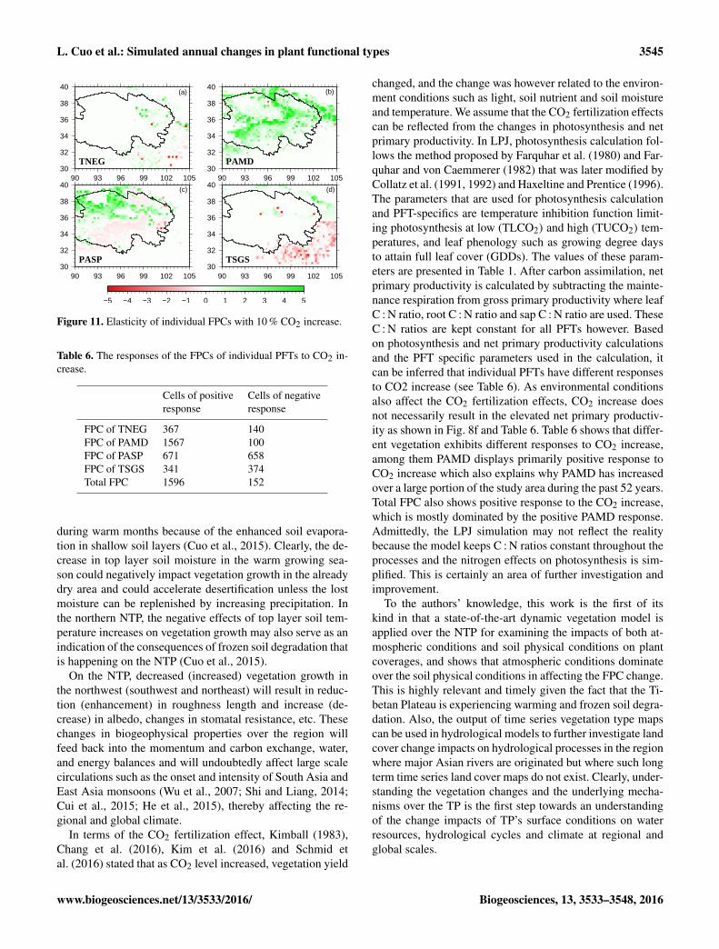
Figure 11. Elasticity of individual FPCs with 10 % CO2 increase.

Table 6. The responses of the FPCs of individual PFTs to CO2 in-crease.

Cells of positive Cells of negativeresponse response

FPC of TNEG 367 140FPC of PAMD 1567 100FPC of PASP 671 658FPC of TSGS 341 374Total FPC 1596 152

during warm months because of the enhanced soil evapora-tion in shallow soil layers (Cuo et al., 2015). Clearly, the de-crease in top layer soil moisture in the warm growing sea-son could negatively impact vegetation growth in the alreadydry area and could accelerate desertification unless the lostmoisture can be replenished by increasing precipitation. Inthe northern NTP, the negative effects of top layer soil tem-perature increases on vegetation growth may also serve as anindication of the consequences of frozen soil degradation thatis happening on the NTP (Cuo et al., 2015).

On the NTP, decreased (increased) vegetation growth inthe northwest (southwest and northeast) will result in reduc-tion (enhancement) in roughness length and increase (de-crease) in albedo, changes in stomatal resistance, etc. Thesechanges in biogeophysical properties over the region willfeed back into the momentum and carbon exchange, water,and energy balances and will undoubtedly affect large scalecirculations such as the onset and intensity of South Asia andEast Asia monsoons (Wu et al., 2007; Shi and Liang, 2014;Cui et al., 2015; He et al., 2015), thereby affecting the re-gional and global climate.

In terms of the CO2 fertilization effect, Kimball (1983),Chang et al. (2016), Kim et al. (2016) and Schmid etal. (2016) stated that as CO2 level increased, vegetation yield

changed, and the change was however related to the environ-ment conditions such as light, soil nutrient and soil moistureand temperature. We assume that the CO2 fertilization effectscan be reflected from the changes in photosynthesis and netprimary productivity. In LPJ, photosynthesis calculation fol-lows the method proposed by Farquhar et al. (1980) and Far-quhar and von Caemmerer (1982) that was later modified byCollatz et al. (1991, 1992) and Haxeltine and Prentice (1996).The parameters that are used for photosynthesis calculationand PFT-specifics are temperature inhibition function limit-ing photosynthesis at low (TLCO2) and high (TUCO2) tem-peratures, and leaf phenology such as growing degree daysto attain full leaf cover (GDDs). The values of these param-eters are presented in Table 1. After carbon assimilation, netprimary productivity is calculated by subtracting the mainte-nance respiration from gross primary productivity where leafC : N ratio, root C : N ratio and sap C : N ratio are used. TheseC : N ratios are kept constant for all PFTs however. Basedon photosynthesis and net primary productivity calculationsand the PFT specific parameters used in the calculation, itcan be inferred that individual PFTs have different responsesto CO2 increase (see Table 6). As environmental conditionsalso affect the CO2 fertilization effects, CO2 increase doesnot necessarily result in the elevated net primary productiv-ity as shown in Fig. 8f and Table 6. Table 6 shows that differ-ent vegetation exhibits different responses to CO2 increase,among them PAMD displays primarily positive response toCO2 increase which also explains why PAMD has increasedover a large portion of the study area during the past 52 years.Total FPC also shows positive response to the CO2 increase,which is mostly dominated by the positive PAMD response.Admittedly, the LPJ simulation may not reflect the realitybecause the model keeps C : N ratios constant throughout theprocesses and the nitrogen effects on photosynthesis is sim-plified. This is certainly an area of further investigation andimprovement.

To the authors’ knowledge, this work is the first of itskind in that a state-of-the-art dynamic vegetation model isapplied over the NTP for examining the impacts of both at-mospheric conditions and soil physical conditions on plantcoverages, and shows that atmospheric conditions dominateover the soil physical conditions in affecting the FPC change.This is highly relevant and timely given the fact that the Ti-betan Plateau is experiencing warming and frozen soil degra-dation. Also, the output of time series vegetation type mapscan be used in hydrological models to further investigate landcover change impacts on hydrological processes in the regionwhere major Asian rivers are originated but where such longterm time series land cover maps do not exist. Clearly, under-standing the vegetation changes and the underlying mecha-nisms over the TP is the first step towards an understandingof the change impacts of TP’s surface conditions on waterresources, hydrological cycles and climate at regional andglobal scales.



In this study, the role of CO2 in FPC changes is discussedsolely in the context of photosynthesis. However, CO2 isa greenhouse gas and increasing CO2 concentrations havebeen credited as one of the primary driving forces behind theglobal warming. Without utilizing a fully coupled dynamicatmosphere-land surface-vegetation model it appears to berather difficult to separate the effects of CO2 between photo-synthesis related and greenhouse gas related.

5 Conclusions

In summary, this study documents the changes in PFTs rep-resented by FPCs on the NTP during the past five decadesand the possible mechanisms behind those changes throughexamining the responses of PFTs to changes in climatevariables of precipitation, air temperature, atmospheric CO2concentrations, 40 cm-deep soil temperature and moisture.Among the five variables, precipitation is found to be themajor factor influencing the total vegetation coverage posi-tively, while root zone soil temperature is the least importantone with negative impacts. About 34 % of the NTP exhibitsincreasing total FPC trends compared to 13 % with decreas-ing trends during 1957–2009. Individual PFTs respond dif-ferently to the changes in the five climate variables. The dif-ferent responses of individual PFTs to climate change giverise to spatially varying patterns of vegetation change. Spa-tially diversified changes in vegetation coverage on the NTPare the result of changes in heterogeneous climatic conditionsin the region, competitions among various PFTs for energyand water, and regional climate-determined bioclimatic re-strictions for the establishment of different PFTs. The effectsof the climate change induced regional plant functional typechanges on water resources and hydrological cycles in oneof the world’s largest and most important headwater regions,on the partition of sensible and latent heat fluxes, and henceon the onset and intensity of south and east Asian monsooncirculations should be examined further.

Data availability

The data sets used in the study include LPJ modelmeteorological forcing, and the model output. Metero-logical forcings temperature and precipitation are avail-able at http://www.tpedatabase.cn/portal/MetaDataInfo.jsp?MetaDataId=249432. Model output data are availablethrough contact with Lan Cuo at [email protected].

Author contributions. Lan Cuo designed the study, conducted thestudy and prepared the manuscripts. Yongxin Zhang provided crit-ical suggestions in the study design and prepared the manuscripts.Shilong Piao helped with the manuscripts. Yanhong Gao providedsuggestions in the study design.

Acknowledgements. This study is supported by the NationalBasic Research Program (grant 2013CB956004), by the NationalNatural Science Foundation of China (grant 41190083), and bythe Hundred Talent Program granted to Lan Cuo by the ChineseAcademy of Sciences. The National Center for AtmosphericResearch (NCAR)’s Advanced Study Program (ASP) is alsoacknowledged for providing partial funding for this work.

Edited by: T. Keenan

References

Ahlstrom, A., Xia, J., Arneth, A., Luo, Y., and Smith, B.: Im-portance of vegetation dynamics for future terrestrial carboncycling, Environ. Res. Lett., 10, 054019, doi:10.1088/1748-9326/10/5/054019, 2015.

Bonan, G. B., Pollard, D., and Thompson, S. L.: Effects of borealforest vegetation on global climate, Nature, 359, 716–718, 1992.

Bonan, G., Levis, S., Sitch, S., Vertenstein, M., and Oleson K. W.:A dynamic global vegetation model for use with climate mod-els: concepts and description of simulated vegetation dynamics,Glob. Change Biol., 9, 1543–1566, 2003.

Ciais, P., Schelhaas, M. J., Zaehle, S., Piao, S. L., Cescatti, A.,Liski, J., Luyssaert, S., LeMaire, G., Schulze, E. D., Bouriaud,O., Freibauer A., Valentini, R., and Nabuurs, G. J.: Carbon accu-mulation in European forests, Nat. Geosci., 1, 425–429, 2008.

Chang, J., Ciais, P., Viovy, N., Vuichard, N., Herrero, M., Havlik,P., Wang, X., Sultan, B., and Soussana, J-F.: Effect of climatechange, CO2 trends, nitrogen addition, and land-cover and man-agement intensity changes on the carbon balance of Europeangrasslands, Glob. Change Biol., 22, 338–350, 2016.

Chen, Z. Q., Shao, Q. Q., Liu, J. Y., and Wang, J. B.: Analysis ofnet primary productivity of terrestrial vegetation on the Qinghai-Tibet Plateau, based on MODIS remote sensing data, ScienceChina: Earth Sciences, 55, 1306–1312, 2012.

Cheng, G. and Jin, H.: Permafrost and groundwater on the Qinghai-Tibet Plateau and in northeast China, Hydrogeol. J., 21, 5–23,2013.

Chinese Academy of Sciences (CAS), 1 : 1 000 000 China Vegeta-tion Map, China Science Publishing & Media Ltd, 2001.

Collatz G. J., Ball, J. T., Grivet C., and Berry J. A.: Physiologi-cal and environmental-regulation of stomatal conductance, pho-tosynthesis and transpiration – a model that includes a laminarboundary-layer, Agr. Forest Meteorol., 54, 107–136, 1991.

Collatz, G. J., Ribas-Carbo, M., and Berry J. A.: Coupledphotosynthesis-stomatal conductance model for leaves of C4plants, Aust. J. Plant Physiol., 19, 519–538, 1992.

Cox, P. M.: Description of the TRIFFID dynamic global vegetationmodel, Hadley Centre Technical Note, 24, 1–16, 2001.

Cui, Y., Duan,A., Liu, Y., and Wu, G.: Interannual variability of thespring atmospheric heat source over the Tibetan Plateau forcedby the North Atlantic SSTA, Clim. Dynam., 45, 1617–1634,2015.

Cuo, L.: Land use/cover change impacts on hydrology in largeriver basins: a review, in: Terrestrial Water Cycle and ClimateChange: Natural and Human-Induced Impacts, edited by: Tang,Q. and Oki, T., American Geophysical Union (AGU) Geophysi-cal Monograph Series, accepted, 2016.


http://www.tpedatabase.cn/portal/MetaDataInfo.jsp?MetaDataId=249432

http://www.tpedatabase.cn/portal/MetaDataInfo.jsp?MetaDataId=249432

http://dx.doi.org/10.1088/1748-9326/10/5/054019

http://dx.doi.org/10.1088/1748-9326/10/5/054019


Cuo, L., Lettenmaier, D. P., Alberti, M., and Richey, J.: Effects of acentury of land cover and climate change on hydrology in PugetSound, Washington, Hydrol. Process., 23. 907–933, 2009.

Cuo, L., Zhang, L., Gao, Y., Hao, Z., and Cairang, L.: The impactsof climate change and land cover transition on the hydrology inthe Upper Yellow River basin, China, J. Hydrol., 502, 37–52,2013a.

Cuo, L., Zhang, Y., Wang, Q., Zhang, L., Zhou, B., Hao, Z., and Su,F.: Climate change on the northern Tibetan Plateau during 1957-2009: spatial patterns and possible mechanisms, J. Climate, 26,85–109, 2013b.

Cuo, L., Zhang, Y., Zhu, F., and Liang, L.: Characteristics andchanges of streamflow on the Tibetan Plateau: A review, Jour-nal of Hydrology: Regional Studies, 2, 49–68, 2014.

Cuo, L., Zhang, Y., Bohn, T.J., Zhao, L., Li, J., Liu, Q., and Zhou,B. Frozen soil degradation and its effects on surface hydrologyin the northern Tibetan Plateau, J. Geophys. Res.-Atmos., 120,8276–8298, 2015.

Dahlin, K. M., Fisher, R. A., and Lawrence, P. J.: Environmen-tal drivers of drought deciduous phenology in the CommunityLand Model, Biogeosciences, 12, 5061–5074, doi:10.5194/bg-12-5061-2015, 2015.

Elsner, M. M., Cuo, L., Voisin, N., Deems, J. S., Hamlet, A. F.,Vano, J. A., Mickelson K. E. B., Lee S.-Y., and Lettenmaier, D.P.: Implications of 21st century climate change for the hydrologyof Washington State, Climatic Change, 102, 225–260, 2010.

FAO: IIASA/ISRIC/ISS-CAS/JRC, Harmonized World SoilDatabase (version 1.0), FAO, Rome, Italy and IIASA, Laxen-burg, Austria, 2008.

Farquhar, G. D., von Caemmerer, S., and Berry, J. A.: Abiochem-ical model of photosynthetic CO2 assimilation in leaves of C3species, Planta, 149, 78–90, 1980.

Farquhar, G. D. and von Caemmerer, S.: Modelling of photosyn-thetic response to environmental conditions, in: Physiologicalplant ecology II: water relations and carbon assimilation, editedby: Nobel, P. S., Osmond, C. B., and Ziegler, H., Springer, Berlin,549–587, 1982.

Fisher, R. A., Muszala, S., Verteinstein, M., Lawrence, P., Xu, C.,McDowell, N. G., Knox, R. G., Koven, C., Holm, J., Rogers,B. M., Spessa, A., Lawrence, D., and Bonan, G.: Taking off thetraining wheels: the properties of a dynamic vegetation modelwithout climate envelopes, CLM4.5(ED), Geosci. Model Dev.,8, 3593–3619, doi:10.5194/gmd-8-3593-2015, 2015.

Gerten, D., Schaphoff, S., Haberlandt, U., Lucht, W., and Sitch, S.:Terrestrial vegetation and water balance-hydrological evaluationof dynamic global vegetation model, J. Hydrol., 286, 249–270,2004.

Haxeltine, A. and Prentice, I. C.: A general model for the light-use efficiency of primary production, Funct. Ecol., 10, 551–561,1996.

He, B., Wu, G., Liu, Y., and Bao, Q.: Astronomical and hydrologicalperspective of mountain impacts on the Asian summer monsoon,Sci. Rep., 5, 17586, doi:10.1038/srep17586, 2015.

Hopcroft, P. O. and Valdes, P. J.: Last glacial maximum constraintson the earth system model HadGEM2-ES, Clim. Dynam., 45,1657–1672, 2015.

Huber, A., and Iroume, A.: Variability of annual rainfall partitionsfor different sites and forest covers in Chile, J. Hydrol., 248, 78–92, 2001.

Jiang, Y., Zhuang, Q., Schaphoff, S., Sitch, S., Sokolov, A., Kick-lighter, D., and Melillo, J.: Uncertainty analysis of vegetation dis-tribution in the northern high latitudes during the 21st century wita dynamic vegetation model, Ecol. Evol., 2, 593–614, 2012.

Jin, Z., Zhuang, Q., He, J., Luo, T., and Shi, Y.: Phenology shiftfrom 1989 to 2008 on the Tibetan Plateau: an analysis with aprocess-based soil physical model and remote sensing data, Cli-matic Change, 119, 435–449, 2013.

Kim, D., Oren, R., and Qian, S. S.: Response to CO2 enrichmentof understory vegetation in the shade of forests, Glob. ChangeBiol., 22, 944–956, 2016.

Kimball, B. A: Carbon dioxide and agricultural yield: an assem-blage and analysis of 430 prior observations, Agr. J., 75,779–788,1983.

Levis, S., Bonan, G. B., Vertenstein, M., and Oleson, K. W.:The community land model’s dynamic global vegetation model(CLM-DGVM): technical description and user’s guide., NCARTechic Note, 459, 1–50, 2004.

Liang, X., Lettenmaier, D. P., and Wood, E. F.: A simple hydrolog-ically based model of land surface water and energy fluxes forgeneral circulation models, J. Geophys. Res., 99, 14415–14428,1994.

Liang, X., Wood, E. F., and Lettenmaier, D. P.: Surface soil moistureparameterization of the VIC-2l model: evaluation and modifica-tion, Global Planet. Change, 13, 195–206, 1996.

Meng, T.-T., Wang, H., Harrison, S. P., Prentice, I. C., Ni, J., andWang, G.: Responses of leaf traits to climatic gradients: adaptivevariation versus compositional shifts, Biogeosciences, 12, 5339–5352, doi:10.5194/bg-12-5339-2015, 2015.

Mengis, N., Keller, D. P., Eby, M., and Oschlies, A.: Uncertainty inthe response of transpiration to CO2 and implications for climatechange, Environ. Res. Lett., 10, 94001–94001, 2015.

Mitchell, T. D. and Jones, P. D.: An improved method of construct-ing a database of monthly climate observations and associatedhigh-resolution grids, Int. J. Climatol., 25, 693–712, 2005.

Murray, S. J.: Trends in 20th century global rainfall interception assimulated by a dynamic global vegetation model: implicationsfor global water resources, Ecohydrology, 7, 102–114, 2014.

Paschalis, A., Fatichi, S., Katul, G. G., and Ivanov, V. Y.: Cross-scale impact of climate temporal variability on ecosystem waterand carbon fluxes, J. Geophys. Res.-Biogeo., 120, 1716–1740,2015.

Pearson, R. G., Phillips, S. J., Loranty, M. M., Beck, P. S. A.,Damoulas, T., Knight, S. J., and Goetz, S. J.: Shifts in Arctic veg-etation and associated feedbacks under climate change, NatureClimate Change, 3, 673–677, doi:10.1038/nclimate1858, 2013.

Peterman, W., Bachelet, D., Ferschweiler, K., and Sheehan, T.: Soildepth affects simulated carbon and water in the MC2 dynamicglobal vegetation model, Ecol. Modell., 294, 84–93, 2015.

Piao, S., Tan, K., Nan, H., Ciais, P., Fang, J., Wang, T., Vuichard,N., and Zhu, B.: Impacts of climate and CO2 changes on the veg-etation growth and carbon balance of Qinghai-Tibetan grasslandsover the past five decades, Global Planet. Change, 98–99, 73–80,2012.

Qiu, J.: China: The third pole, Nature, 454, 393–396, 2008.Reiter, E. R. and Gao, D. Y.: Heating of the Tibet Plateau and move-

ments of the South Asian high during spring, Mon. Weather Rev.,110, 1694–1711, 1982.


http://dx.doi.org/10.5194/bg-12-5061-2015

http://dx.doi.org/10.5194/bg-12-5061-2015

http://dx.doi.org/10.5194/gmd-8-3593-2015

http://dx.doi.org/10.1038/srep17586

http://dx.doi.org/10.5194/bg-12-5339-2015

http://dx.doi.org/10.1038/nclimate1858


Rogers, B. M., Randerson, J. T., and Bonan, G. B.: High-latitude cooling associated with landscape changes from NorthAmerican boreal forest fires, Biogeosciences, 10, 699–718,doi:10.5194/bg-10-699-2013, 2013.

Sankarasubramanian, A., Vogel R. M., and Limbrunner J. F.: Cli-mate elasticity of streamflow in the United States, Water Resour.Res., 37, 1771–1781, 2001.

Sato, H., Itoh, A., and Kohyama, T.: SEIB–DGVM: A new Dy-namic Global Vegetation Model using a spatially explicit indi-vidualbased approach, Ecol. Modell., 200, 279–307, 2007.

Schmid, I., Franzaring, J., Muller, M., Brohon, N., Calvo, O. C.,Hogy, P., and Fangmerier, H.: Effects of CO2 enrichment anddrought on photosynthesis, growth and yield of and old and amodern barley cultivar, J. Agr. Crop Sci., 202, 81–95, 2016.

Shi, Q. and Liang, S.: Surface-sensible and latent heat fluxesover the Tibetan Plateau from ground measurements, reanal-ysis, and satellite data, Atmos. Chem. Phys., 14, 5659–5677,doi:10.5194/acp-14-5659-2014, 2014.

Sitch, S., Smith, B., Prentice, I. C., Arneth, A., Bondeau, A.,Cramer, W., Kaplan, J. O., Levis, S., Lucht, W., Sykes, M. T.,Thonicke, K., and Venevsky, S.: Evaluation of ecosystem dynam-ics, plant geography and terrestrial carbon cycling in the LPJ dy-namic global vegetation model, Glob. Change Biol., 9, 161–185,2003.

Sitch, S., Brovkin, V., Von Bloh, W., Van Vuuren, D., and Eick-hout, B.: Impacts of future land cover changes on atmo-spheric CO2 and climate, Global Biogeochem. Cy., 19, GB2013,doi:10.1029/2004GB002311, 2005.

Sitch, S., Huntingford, C., Gedney, N., Levy, P. E., Lomas, M., Piao,S. L., Betts, R., Ciais, P., Cox, P., Friedlingstein, P., Jones, C.D., Prentice, I. C., and Woodward, F. I.: Evaluation of the ter-restrial carbon cycle, future plant geography and climate-carboncycle feedbacks using five Dynamic Global Vegetation Models(DGVMs), Glob. Change Biol., 14, 2015–2039, 2008.

Sitch, S., Friedlingstein, P., Gruber, N., Jones, S. D., Murray-Tortarolo, G., Ahlström, A., Doney, S. C., Graven, H., Heinze,C., Huntingford, C., Levis, S., Levy, P. E., Lomas, M., Poul-ter, B., Viovy, N., Zaehle, S., Zeng, N., Arneth, A., Bonan,G., Bopp, L., Canadell, J. G., Chevallier, F., Ciais, P., Ellis,R., Gloor, M., Peylin, P., Piao, S. L., Le Quéré, C., Smith, B.,Zhu, Z., and Myneni, R.: Recent trends and drivers of regionalsources and sinks of carbon dioxide, Biogeosciences, 12, 653–679, doi:10.5194/bg-12-653-2015, 2015.

Smith, B., Prentice, I. C., and Sykes, M. T.: Representation ofvegetation dynamics in the modeling of terrestrial ecosystems:comparing two contrasting approaches within European climatespace, Global Ecol. Biogeogr., 10, 621–637, 2001.

Smithwick, E. A. H., Ryan, M. G., Kashian, D. M., Romme, W. H.,Tinker, D. B., and Turner, M. G.: Modeling the effects of fire andclimate change on carbon and nitrogen storage in lodgepole pine(Pinus contorta) stands, Glob. Change Biol., 15, 535–548, 2009.

Steinkamp, J. and Hickler, T.: Is drought-induced forest diebackglobally increasing?, J. Ecol., 103, 31–43, 2015.

Swank, W. T. and Douglass, J. E.: Streamflow greatly reduced byconverting deciduous hardwood stands to pine, Science, 185,857–859, 1974.

Tatarinov, F. A. and Cienciala, R.: Application of BIOME-BGCmodel manage forests 1: sensitivity analysis, Forest Ecol. Man-age., 237, 267–279, 2006.

Wang, B., Bao, Q., Hoskins, B., Wu, G., and Liu, Y.: Tibetan Plateauwarming and precipitation changes in East Asia, Geophys. Res.Lett., 35, L14702, doi:10.1029/2008GL034330, 2008.

Wang, X., Cheng, G., and Zhong, X.: Assessing potential impactsof climatic change on subalpine forests on the eastern TibetanPlateau, Climatic Change, 108, 225–241, 2011.

Weiss, M., Miller, P. A., van den Hurk, B. J. J. M., van Noije T.,Tefanescu, S. S., Haarsma, R., van Ulft, L. H., Hazeleger, W.,Le Sager, P., Smith, B., and Schurgers, G.: Contribution of dy-namic vegetation phenology to decadal climate predictability, J.Climate, 27, 8563–8577, 2014.

Wigmosta, M.S., Vail, L. W., and Lettenmaier, D. P.: A distributedhydrology vegetation model for complex terrain, Water Resour.Res., 30, 1665–1679, 1994.

Wu, G. X., Liu, Y., Wang, T., Wan, R., Liu, X., Li, W., and Liang, X.:The influence of mechanical and thermal forcing by the TibetanPlateau on Asian climate, J. Hydrometeorol., 8, 770–789, 2007.

Yanai, M., Li, C., and Song, Z.: Seasonal heating of the TibetanPlateau and its effects on the evolution of the summer monsoon,J. Meteorol. Soc. Japan, 70, 319–351, 1992.

Ye, D. Z. and Wu, G. X.: The role of the heat source of the TibetanPlateau in the general circulation, Meteorol. Atmos. Phys., 67,181–198, 1998.

Yeh, T. C. and Gao, Y. X.: The Meteorology of the Qinghai-Xizang(Tibet) Plateau, edited by: Yeh, T.-C. and Gao, Y.-X., SciencePress, Beijing, China, 278 pp., 1979 (in Chinese).

Zhang, Y., Li, T., and Wang, B.: Decadal change of the spring snowdepth over the Tibetan Plateau: The associated circulation andinfluence on the East Asian summer monsoon, J. Climate, 17,2780–2793, 2004.

Zhang, Y., Wang, X., Hu, R., Pan, Y., and Paradeloc, M.: Rain-fall partitioning into throughfall, stemflow and interception lossby two xerophytic shrubs within a rain-fed re-vegetated desertecosystem, northwest China, J. Hydrol., 527, 1084–1095, 2015.

Zheng, D., Yang, Q. Y., and Wu, S. H.: Eco-geographical RegionSystem of China, Beijing: The Commercial Press, 2008 (in Chi-nese).

Zhong, L., Ma, Y., Suhyb, S. M., and Su, Z.: Assessment of vege-tation dynamics and their response to variations in precipitationand temperature in the Tibetan Plateau, Climatic Change, 103,519–535, 2010.


http://dx.doi.org/10.5194/bg-10-699-2013

http://dx.doi.org/10.5194/acp-14-5659-2014

http://dx.doi.org/10.1029/2004GB002311

http://dx.doi.org/10.5194/bg-12-653-2015

http://dx.doi.org/10.1029/2008GL034330

Documents

Simulated annual changes in plant functional types and ... · Simulated annual changes in plant functional types and their ... (TP) exerts strong ... and the partition of net radiation