1

Simulating Buoyancy-Driven Airflow in Buildings by 1

Coarse-Grid Fast Fluid Dynamics 2

Mingang Jin1, Wei Liu2,1, Qingyan Chen2,1* 3

1School of Mechanical Engineering, Purdue University, West Lafayette, IN 47907, USA 4 2School of Environmental Science and Engineering, Tianjin University, Tianjin 300072, China 5

*Tel. (765)496-7562, Fax (765)494-0539, Email: yanchen@purdue.edu6

7 Abstract 8

Fast fluid dynamics (FFD) is an intermediate model between multi-zone models and 9 computational fluid dynamics (CFD) models for indoor airflow simulations. The use of coarse 10 grids is preferred with FFD in order to increase computing speed. However, by using a very large 11 mesh cell to represent a heat source that could have a much smaller physical size than the cell, 12 coarse-grid FFD would under-predict the thermal plume and thermal stratification. This 13 investigation integrated a thermal plume model into coarse-grid FFD. The integration first used 14 the plume model to calculate a source for the momentum equations and then corrected the 15 temperature at the plume cell. The integration enabled coarse-grid FFD to correctly predict the 16 plumes. When applied to displacement ventilation, coarse-grid FFD with the plume model can 17 accurately predict the mean air temperature stratification in rooms as compared with 18 experimental data from the literature. The improved model has also been used to calculate the 19 ventilation rate for buoyancy-driven natural ventilation. The calculated ventilation rates agree 20 well with the experimental data or predictions by CFD and analytical models. Coarse-grid FFD 21 with the plume model used only a small fraction of the computing time required by fine-grid 22 FFD, while the associated errors for the two grid sizes were comparable. 23

Keywords: Heat sources, plume model, computational fluid dynamics, experimental validation, 24 analytical model 25

Research highlights 26

This study integrated a thermal plume model into coarse-grid FFD.27

The integrated model was tested with buoyancy-driven airflow in buildings.28

The plume model can improve representing the heat source with very coarse cell.29

The integrated model used less computing time but maintained reasonable accuracy.30

31

32

Jin, M., Liu, W. and Chen, Q. 2015. “Simulating buoyancy-driven airflow in buildings by coarse-grid fast fluid dynamics,” Building and Environment, 85, 144-152.

2

1. Introduction 33

Whole-building airflow simulations are required in applications such as natural ventilation 34 design, coupled building airflow and energy simulation, smoke control, and air quality diagnosis 35 in a building. These simulations generally use multi-zone models [1]. However, the models can 36 provide only very limited airflow information because of the assumption that a room within a 37 building can be treated as a single homogeneous node. Computational Fluid Dynamics (CFD) 38 models, on the other hand, can perform detailed airflow simulations, but the use of CFD for 39 whole-building airflow simulations is too computationally expensive [2]. Between CFD models 40 and multi-zone models, researchers have also developed intermediate models for whole-building 41 airflow simulations. Zonal models [3] are typical intermediate models that can achieve a balance 42 between reduced computing costs and the level of detail required in airflow simulations. 43 Additionally, by using very coarse grids, coarse-grid CFD models [4] can provide more detailed 44 airflow simulations at a competitive computing speed with respect to zonal models, and they are 45 expected to replace zonal models in the future [2]. Fast Fluid dynamics (FFD), a recently 46 developed intermediate model that can provide reliable simulations of indoor airflows at a speed 47 that is about 15 times faster than CFD models, currently has great potential for performing 48 whole-building airflow simulations [5, 6]. Because FFD is also a grid-based model, reducing the 49 grid number can further enhance the computing speed of FFD simulations. Coarse-grid FFD 50 would be an ideal tool for performing whole-building airflow simulations at a greatly reduced 51 computing cost. 52

Although a coarse grid could significantly reduce the computing time of FFD simulations, it may 53 cause problems in the representation of the boundary conditions encountered in building airflow 54 simulations. For example, many heat sources in buildings are of small physical size, such as 55 computers, desk lamps, occupants, etc. Using a very large mesh cell to represent a small-sized 56 heat source would result in the prediction of lower energy intensity in the cell and smaller 57 buoyancy forces from the heat source. Coarse-grid FFD would thus tend to under-predict the 58 plume flow generated by the heat source and would not accurately predict buoyancy-driven 59 ventilation and room air temperature distribution. Because buoyancy-driven ventilation is a 60 major feature of high-performance building systems, such as displacement ventilation and 61 buoyancy-driven natural ventilation systems, correct prediction of buoyancy-driven ventilation 62 and room air temperature distribution is essential with coarse-grid FFD. 63

Thus it is necessary to improve the representation of small heat sources with large cells. In CFD 64 models, simulations are normally performed on fine grids, which allows CFD models to avoid 65 the aforementioned problem. Instead, to reduce the complexities of representing heat sources in 66 simulations, it is still necssary for CFD models to apply simple heat source geometries or use 67 replacement boundary conditions [7]. As intermediate models, zonal models also have the same 68 problem of reprezenting heat sources as coarse-grid FFD does. Thus the approaches applied in 69 zonal models to model thermal plumes could also be a potential solution for coarse-grid FFD. 70

3

Extensive research has been conducted into the characteristics of thermal plumes [8]. Morton et 71 al. [9] proposed a theoretical model to describe the physics of thermal plumes, and this model 72 has been adapted for studying a wide variety of thermal plumes. Kofoed [10] experimentally 73 studied thermal plumes generated by indoor heat sources in ventilated rooms and proposed a 74 model coefficient to account for the influence of enclosing walls. Trzeciakiewicz [11] 75 experimentally investigated the characteristics of thermal plumes in response to objects of 76 varying shape, such as computers, desk lamps, and light bulbs. The investigation revealed that 77 the experimentally determined model of a plume above a point heat source could be used to 78 characterize the thermal plumes in displacement ventilation. Zukowska et al. [12] investigated 79 the characteristics of the thermal plume generated by a sitting person using four different 80 geometries and found that a rectangular box could correctly simulate the enthalpy flux and 81 buoyancy flux generated by the person. Craven and Settles [13] performed a computational and 82 experimental investigation to characterize the thermal plume from a person and concluded that 83 the room temperature stratification had a significant effect on plume behavior. The 84 aforementioned research into the characteristics of indoor thermal plumes has provided a wealth 85 of information. 86

On the basis of these studies of thermal plume physics and analytical plume models, simple 87 models have been developed to quantify ventilation and temperature distributions in buildings 88 [14, 15]. In addition, plume models have been used to improve the performance of other models 89 for simulating buoyancy-driven airflows in buildings. Inard et al. [16] integrated a wall thermal 90 plume model into a zonal model to improve the latter’s performance in simulating the 91 temperature distribution in a room. Musy et al. [17] integrated a plume model with a zonal model 92 to obtain a better simulation of natural convection in a room with a radiative-convective heater. 93 Stewart and Ren [18] used a plume model to improve the simulation accuracy of a zonal model 94 for studying the airflow rising from a cooking plate. It has been shown that plume models 95 effectively enhance the performance of zonal models in simulating buoyancy-driven airflows in 96 buildings. 97

The integration of plume models with zonal models suggests that plume models could also be 98 integrated with FFD for improving the performance of coarse-grid FFD simulations for room 99 airflows driven by heat sources. This study therefore developed a method of implementing a 100 plume model in FFD when the mesh cell is much larger than the heat source. The proposed 101 integration method was also tested and evaluated. 102

103

2. Research Method 104

2.1 Fast fluid dynamics 105

FFD simulates an airflow by numerically solving a set of partial differential equations 106 representing the transport phenomena in the airflow, Eq. (1)-(3), which are derived on the basis 107

4

of the conservation of mass, momentum (Navier-Stokes equations), and scalar transport 108 quantities (such as energy and species), respectively. 109

0,i

i

U

x

(1) 110

21 1

,i i ij i

j i j j

U U UpU F

t x x x x

(2) 111

2

,jj j j

U St x x x

(3) 112

where i or j = 1, 2, 3; Ui is the ith component of the velocity vector, xi the ith direction of 113 coordinate, t time, p pressure, ρ density, ν the kinetic viscosity, Fi the ith component of the body 114 forces, the scalar variables, Γ the transport coefficient for , and S the source term. In each 115

time step, FFD solves this set of transport equations sequentially. To enhance computational 116 efficiency, a time-splitting scheme [19] was applied to solve the transport equations. For 117 example, FFD splits the scalar transport equation (3) into an advection equation (4) and a 118 diffusion equation (5), 119

(1)

,n n

jj

Ut x

(4) 120

1 (1) 2 1

2,

n n

j

St x

(5) 121

where n and 1n represent the variable at the current and next time steps, respectively, and (1)122

represents the intermediate variables solved by the advection equation. The advection equation 123 (4) is first solved with the conservative semi-Lagrangian scheme [20] to obtain the intermediate 124

value (1) , and then FFD is implicitly solved using the diffusion equation (5) to update the scalar 125

distribution at the next time step. To effectively resolve the coupling between the momentum 126 equations and the continuity equation, a pressure projection [21] is performed force the velocity 127 field to satisfy continuity. 128

2.2 Integration with plume model 129

As a result of natural convection, air surrounded by a heat source in a room can form a buoyancy 130 plume. As the plume rises, it induces the surround air into the plume flow, and flow carries the 131 heat from the heat source to the upper part of the room. To describe the features of buoyancy-132

driven airflows, the plume flow rate ( pV ) and excess temperature ( pT ) in the plume region are 133

usually the two most important parameters [22], and they vary with the heat generation rate, heat 134 source geometry, heat source location, etc. When the mesh cell size used in coarse-grid FFD is 135

5

much larger than the physical size of a heat source, the two parameters predicted by FFD may 136 not be accurate. In order to improve the performance of coarse-grid FFD in predicting the 137 thermal plume, this study used an analytical plume model with empirical coefficients to calculate 138 the plume flow rate and the excess temperature in the plume region. The two calculated 139 parameters were then integrated into FFD in order to represent the heat source. 140

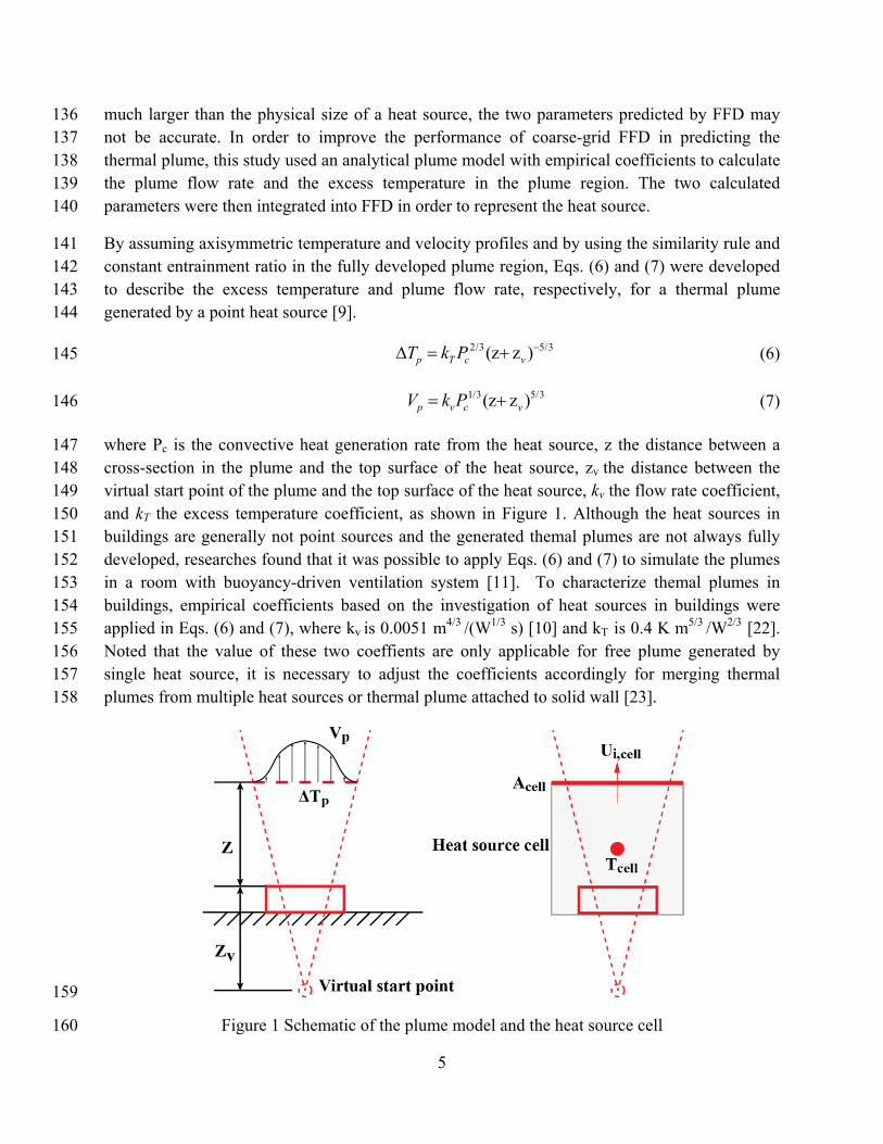
By assuming axisymmetric temperature and velocity profiles and by using the similarity rule and 141 constant entrainment ratio in the fully developed plume region, Eqs. (6) and (7) were developed 142 to describe the excess temperature and plume flow rate, respectively, for a thermal plume 143 generated by a point heat source [9]. 144

2/3 5/3(z z )p T c vT k P (6) 145

1/3 5/3(z z )p v c vV k P (7) 146

where Pc is the convective heat generation rate from the heat source, z the distance between a 147 cross-section in the plume and the top surface of the heat source, zv the distance between the 148 virtual start point of the plume and the top surface of the heat source, kv the flow rate coefficient, 149 and kT the excess temperature coefficient, as shown in Figure 1. Although the heat sources in 150 buildings are generally not point sources and the generated themal plumes are not always fully 151 developed, researches found that it was possible to apply Eqs. (6) and (7) to simulate the plumes 152 in a room with buoyancy-driven ventilation system [11]. To characterize themal plumes in 153 buildings, empirical coefficients based on the investigation of heat sources in buildings were 154 applied in Eqs. (6) and (7), where kv is 0.0051 m4/3 /(W1/3 s) [10] and kT is 0.4 K m5/3 /W2/3 [22]. 155 Noted that the value of these two coeffients are only applicable for free plume generated by 156 single heat source, it is necessary to adjust the coefficients accordingly for merging thermal 157 plumes from multiple heat sources or thermal plume attached to solid wall [23]. 158

159

Figure 1 Schematic of the plume model and the heat source cell 160

6

The integration of the plume model with FFD was divided into two parts: integration with the 161 momentum equations and with the energy equation. Because coarse-grid FFD cannot correctly 162 predict the plume flow rate driven by the heat source, Eq. (7) was used to estimate the airflow 163 rate of the plume at the heat source cell. Dividing the flow rate by the area of the horizontal cell 164

surface cellA provided an estimate of the velocity component in the plume direction ,plumeiU for 165

the heat source cell, 166

,plume /i p cellU V A . (8) 167

The plume velocity ,plumeiU was compared with the vertical velocity component ,ni cellU of the heat 168

source cell at the previous time step in order to determine the amount of correction required for 169

adjusting the velocity at the heat source cell. On the basis of the difference between ,plumeiU and 170

,ni cellU , the momentum source or sink was calculated and was incorporated into the momentum 171

equations as a source term, as shown in Equation (9), 172

, , ,plume ,( ) / ,ni cell i cell i i cellF F U U t (9) 173

where ,i cellF is the body force term in the heat source cell and t the time step size. When the 174

momentum source term in the cell is incorporated the plume velocity at the cell can be corrected 175 to be the same as that in the analytical model. 176

For integration with the energy equation, the plume model was used to adjust the air temperature 177 at the heat source cell because FFD underestimates the heat source temperature when a very 178 coarse grid is used. To minimize the impact of the temperature correction on the energy 179 conservation in the domain, the correction was applied in the advection process and before the 180 energy conservation correction of the semi-Lagragian scheme. Therefore, a three-step approach 181 was applied to solve the advection equation for energy transport: 182

* ( ),ncell cellcellT T x tU

(10) 183

** * ( ),n n

cell cell p ambient cellT T T T T (11) 184

(1) ** ,cell cell cellT T (12) 185

where, cellx

represents the coordinates of the heat source cell, cellU

the velocity vector at the 186

heat source cell, t the time step size, nT the temperature at the previous time step, (1)T the 187

temperature solved by the advection equation, ambientT the air temperature away from the plume 188

region, the correction weighting factor, and the energy imbalance rate. To solve the 189

advection equation for temperature at the cell, the standard semi-Lagrangian scheme was first 190

7

applied to obtain intermediate temperature *T from Eq. (10). Next, on the basis of the excess 191 temperature calculated by the plume model, a correction was conducted for the temperature at 192

the cell in order to obtain corrected intermediate temperature **T by using Eq. (11). FFD then 193 applied the energy conservation correction (Eq. (12)) to obtain the cell temperature after 194 advection. 195

When the plume model has been integrated into the momentum and energy equations according 196 to the procedure described above, FFD with coarse grids can correctly predict the airflow and 197 temperature in the heat source cell. Furthermore, the simulation is stable, and the airflow is 198 conservative. 199

3. Results 200

Using the integrated plume model, this study applied coarse-grid FFD to simulate building 201 airflows driven by heat sources, including displacement ventilation in a chamber with a heated 202 box, displacement ventilation in an occupied office, buoyancy-driven single-sided natural 203 ventilation, and buoyancy-driven natural ventilation in an atrium. To evaluate the performance of 204 the plume model in representing heat sources in the coarse-grid simulations, the mean vertical air 205 temperature distribution and the ventilation rate predicted by FFD with and without the plume 206 model were compared with the corresponding experimental data or analytical solution. In 207 addition, this study compared the simulation accuracy of FFD with coarse and fine grids. 208

3.1 Displacement ventilation in a chamber with a heated box 209

This study first applied FFD to simulate displacement ventilation with a single heat source and 210 compared the simulated results with the experimental data obtained by Li et al. [24]. Figure 211 2shows the test chamber with dimensions of 4.2 m × 3.6 m × 2.75 m inside a laboratory. Air at a 212 temperature of 18 oC and ventilation rate of 125 m3/h was supplied by a diffuser with dimensions 213 of 0.5 m × 0.45 m located on the side wall of the test chamber at floor level. An air exhaust with 214 dimensions of 0.525 m × 0.22 m was located on the front wall at ceiling level. A 300-W cubic 215 heat source with dimensions of 0.4 m × 0.3 m × 0.3 m was placed on the floor in the center of the 216 test room. Table 1 shows the measured temperatures of the chamber’s interior surfaces. 217

218

8

219

Figure 2 Geometry of the test chamber with displacement ventilation inside a laboratory [24] 220

221

Table 1 Temperatures of the chamber’s interior surfaces [24] 222

Surface Floor Side walls at different heights

Ceiling 0.5 m 1.0 m 1.5 m 2.0 m 2.5 m

Temperature (K) 295.1 295 295.7 296.5 296.8 296.8 298.2

223

In the coarse-grid FFD simulations, the test chamber was represented by a total grid number of 5 224 × 5 × 5. Because the mesh cells were very large, the dimensions of the mesh cell containing the 225 heat source were 0.72 m × 0.55 m × 0.84 m. The cell size was almost ten times the physical size 226 of the heat source. This study simulated the temperature distribution in the test chamber with and 227 without the use of the plume model to represent the heat source. In addition, fine-grid FFD with 228 a grid number of 20 × 20 × 20 was applied to simulate the plume generation and temperature 229 stratification in the test chamber. 230

Figure 3presents the temperature distribution and velocity field at the vertical mid-plane of the 231 chamber as predicted by FFD with and without the plume model. Without the plume model, as 232 shown in Figure 3(b), FFD predicted a smaller thermal plume. This is because the large cell used 233 for the heat source would have a lower mean air temperature than that in the actual plume. 234 Because of the reduced air temperature, the plume flow rate was also lower, and there was less 235 air entrainment from the surroundings. However, with the plume model as depicted in Figure 236 3(a), the predicted air entrainment was much greater. Because the energy intensity was reduced 237 in the large heat source cell, FFD without the plume model predicted an unrealistically low air 238 temperature in the plume region, as illustrated by Figure 3b). For example, the air temperature in 239 the plume region was even lower than that at ceiling level. The model correctly predicted the 240

9

high air temperature near the ceiling that was caused by the rising thermal plume, as shown in 241 Figure 3(a). 242

243

(a) (b) 244

Figure 3 The air temperature and velocity distribution at the vertical mid-plane of the test 245 chamber as predicted by FFD (a) with the plume model and (b) without the plume model 246

247

This study further examined the mean air temperature distribution at different heights in the test 248 chamber as predicted by coarse-grid FFD. Figure 4 compares the temperature profile predicted 249 by course-grid FFD with those from fine-grid FFD and the data measured by Li et al. [24]. FFD 250 without the plume model under-predicted the temperature stratification in the chamber, and it 251 predicted temperatures that were too low in the upper part of the chamber and too high at floor 252 level. Coarse-grid FFD with the plume model produced a temperature profile that agrees much 253 better with the experimental data, except in the region near the floor. Because the temperature 254 gradient near the floor was high, the grid resolution used by coarse-grid FFD was too low to 255 accurately reflect the large temperature variation in this region. Fine-grid FFD provided a 256 slightly better prediction of the temperature profile near the floor. Due to the averaging of the 257 temperature at the same hight, the discrepency between the temperature profiles predicted by two 258 models was not as apprant as observed in Figure 3. But it was still obvious that the plume model 259 improved FFD’s prediction of thermal plume [24]. Coarse-grid FFD with the plume model was 260 able to simulate the temperature stratification with an acceptable accuracy for engineering 261 applications. 262

10

263

Figure 4 Comparison of the mean vertical air temperature profiles in the chamber as predicted by 264 coarse-grid FFD with and without the plume model and by fine-grid FFD, as well as the 265 measured profile. 266

267

3.2 Displacement ventilation in an occupied office 268

To evaluate the performance of the plume model for improving the accuracy of coarse-grid FFD 269 in simulating thermal plumes, this study next investigated airflows in an occupied office space 270 with displacement ventilation. An office mock-up with dimensions of 5.16 m × 3.65 m × 2.43 m 271 was used by Yuan et al. [25] for experimental measurements, as shown in Figure 5(a). Air at a 272 temperature of 17.0 oC was supplied through a displacement diffuser on the side wall at floor 273 level at a ventilation rate of 183.1 m3/h. The air was exhausted through an outlet located in the 274 center of the ceiling. Two heated dummies with dimensions of 0.4 m × 0.4 m × 0.7 m to simulate 275 occupants, and two heated boxes with dimensions of 0.4 m × 0.4 m × 0.4 m to simulate 276 computers, were placed in the chamber as heat sources. These heat sources generated thermal 277 plumes that reached the upper part of the room. The experiment by Yuan et al. [25] measured the 278 air temperature along nine vertical poles distributed in the streamwise center plane (P1–P5) and 279 the cross-sectional center plane (P6-P9), as shown in Figure 5(b). 280

11

281

(a) (b) 282

Figure 5 (a) Schematic of the office with displacement ventilation and (b) the measurement 283 locations 284

285

The coarse-grid FFD simulations used 5 × 5 × 8 mesh cells to represent the office, as shown in 286 Figure 6. Since the mesh was very coarse, two of the cells contained heat sources, and each 287 contained an occupant and a nearby computer on a desk. Each heat source cell had dimensions of 288 0.7 m × 0.75 m × 0.75 m. Once again, the simulations were performed by coarse-grid FFD with 289 and without the plume model and by fine-grid FFD with a cell number of 20 × 20 × 20. 290

291

Figure 6 Coarse grid used to represent an office with two heat sources 292

12

293

Figure 7 compares the vertical air temperature distribution at five locations (PI-P5) predicted by 294 coarse-grid and fine-grid FFD with the experimental data. The results at the other measured 295 locations (P6-P9) were similar, but they are not presented here because of the limited space 296 available in this paper. Coarse-grid FFD without the plume model could not correctly predict the 297 air temperature profiles as compared with the experimental data. Because the thermal plumes 298 were artificially weakened by the use of a large cell to represent the heat sources, the amount of 299 energy transported to the upper part of the room was significantly reduced. Thus, in the upper 300 part of the office the predicted air temperature was lower than that measured experimentally. 301 However, the use of the plume model to represent heat sources improved the accuracy of the 302 coarse-grid FFD in simulating the buoyancy flows driven by the heat sources and thus provided a 303 better prediction of the vertical air temperature profiles. In addition, the simulation results proved 304 the viability of combining several adjacent heat sources into a single heat source so that the 305 plume model could be used. Interestingly, coarse-grid FFD can predict the air temperature 306 profiles with accuracy similar to that of fine-grid FFD. 307

308

13

Figure 7 Comparison of the vertical air temperature profiles at five positions (P1-P5) as predicted by various FFD models and according to experimental data from Yuan et al. [25]

(T-Ts)/(Tr-Ts)

Z/H

0.4 0.6 0.8 1 1.20

0.2

0.4

0.6

0.8

1

P4

(T-Ts)/(Tr-Ts)

Z/H

0 0.2 0.4 0.6 0.8 1 1.20

0.2

0.4

0.6

0.8

1

P1

(T-Ts)/(Tr-Ts)Z

/H0.2 0.4 0.6 0.8 1 1.20

0.2

0.4

0.6

0.8

1

P3

(T-Ts)/(Tr-Ts)

Z/H

0.4 0.6 0.8 10

0.2

0.4

0.6

0.8

1

P5

(T-Ts)/(Tr-Ts)

Z/H

0.2 0.4 0.6 0.8 1 1.20

0.2

0.4

0.6

0.8

1

P2

EXP Fine-grid FFDWith Plume ModelWithout Plume Model

14

3.3 Buoyancy-driven single-sided natural ventilation 309

Following the successes in the displacement ventilation cases, this study applied the coarse-grid 310 FFD to more challenging cases, such as buoyancy-driven natural ventilation, where flow rate is 311 determined by thermal plumes. The case selected for buoyancy-driven natural ventilation in this 312 study was taken from Jiang and Chen [26], who used a test chamber with dimensions of 5.34 m 313 × 3.57 m × 2.46 m inside a laboratory to simulate the indoor environment, and the surrounding 314 laboratory space to simulate the outdoor environment, as shown in Figure 8(a). The thermal 315 plume was generated by a 1500-W baseboard heater with dimensions of 0.16 m × 0.2 m × 0.7 m 316 that was placed on the floor in close proximity to the interior wall. An open door was used to 317 simulate the single-sided opening where natural ventilation occurred. Because the walls of the 318 test chamber and environmental chamber were of very high insulation value, they were 319 considered to be adiabatic. Jiang and Chen measured the vertical air temperature profiles at five 320 different locations, as shown in Figure 8(b), as well as the ventilation rates in the test chamber. 321 Table 2 shows the enclosure surface temperatures of the laboratory as measured by Jiang and 322 Chen. 323

Table 2 Enclosure surface temperatures of the laboratory 324

Ceiling Floor North wall South wall East wall West wall

Temperature (K) 296.11 295.11 296.01 295.90 293.94 295.83

325

326

327

(a) (b) 328

Figure 8 (a) Sketch of experimental setup and (b) measurement positions inside and outside the 329 test chamber 330

331

15

Our coarse-grid FFD used 18 × 10 × 10 mesh cells to represent the entire laboratory, while 6 × 6 332 × 6 cells were used for the test chamber, and a single cell of 0.3 m × 0.64 m × 0.7 m was used for 333 the baseboard heater. Note that the latter cell was much larger than the physical size of the 334 heater. In addition, the entire laboratory in this case was simulated by FFD with a fine grid of 30 335 × 20 × 20. 336

Figure 9 compares the vertical air temperature profiles simulated by coarse-grid FFD with and 337 without the plume model and by fine-grid FFD, with the experimental data at positions P1, P2, 338 P3, and P5. The temperature profiles predicted by coarse-grid FFD with the plume model and by 339 fine-grid FFD were in very good agreement with the measured profiles. Coarse-grid FFD without 340 the plume model resulted in temperature profiles that did not agree as well with the experimental 341 data. The model predicted a lower air temperature in the upper part of the room because of the 342 weaker–than-actual thermal plume predicted by the cell that was much larger than the heater. 343

Because the buoyancy flow generated by the heater was the primary driving force for the airflow 344 in the chamber, correct simulation of the thermal plume was crucial for the prediction of the 345 ventilation rate through the door opening. Table 3 compares the ventilation rates computed by 346 coarse-grid FFD with and without the plume model and by fine-grid FFD, with the experimental 347 data. Some uncertainties were observed in the measured data for this case. They resulted from 348 instabilities in the natural ventilation system, which caused the ventilation rate to vary from 9.18 349 to 12.6 ACH. Because of the reduced heat source intensity in the large heat source cell, a small 350 plume was predicted by the coarse-grid FFD without the plume model. As a result, the predicted 351 ventilation rate was low in comparison with the lowest measured ventilation rate. Both the 352 coarse-grid FFD with the plume model and the fine-grid FFD can accurately predict the 353 ventilation rate caused by the thermal plume from the heater in the chamber. Coarse-grid FFD 354 with the plume model predicted a ventilation rate that was equal to the mean value in the 355 experiment. 356

Table 3 Ventilation rates for the buoyancy-driven, single-side natural ventilation case obtained 357 from various models and the experiment by Jiang and Chen [26]. 358

359

Experiment Fine-grid FFD

Coarse-grid FFD

Without plume model

With plume model

Ventilation rate (ACH)

9.18-12.6 9.36 7.4 10.6

16

Figure 9 Comparison of the vertical air temperature profiles predicted by various FFD models with the experimental data from Jiang and Chen [26].

Temperature (K)

H(m

)

290 295 300 3050

0.5

1

1.5

2

P2

Temperature (K)

H(m

)

290 295 300 3050

0.5

1

1.5

2

P3

Temperature (K)

H(m

)

290 295 300 3050

0.5

1

1.5

2

P1

EXP Without Plume Model Fine-grid FFDWith Plume Model

Temperature (K)

H(m

)

290 295 300 3050

0.5

1

1.5

2

P5

17

3.4 Buoyancy-driven natural ventilation in an atrium 360

This study also applied FFD to the simulation of buoyancy-driven natural ventilation in an 361 atrium, which is a major feature of modern natural ventilation designs for buildings. A tool that 362 predicts the ventilation rate of buoyancy-driven airflow through an atrium with reasonable 363 accuracy would effectively help architects improve natural ventilation designs. To test the 364 performance of coarse-grid FFD in simulating atrium-assisted natural ventilation, this study 365 simulated buoyancy-driven natural ventilation flows in a single-storey space connected to an 366 atrium [27]. 367

Figure 10 shows a case in which a scaled building shell of 2.5 m (W) × 6.5 m (L) × 1.58 m (H) 368 was connected to an atrium with a height of 3.71 m (M). A heat source of 100 W was placed in 369 the center of the building to generate a buoyancy force. The building was ventilated through a 370 top-down chimney (TDC) located near the left wall. An opening was constructed in the ceiling of 371 the building shell connected to the atrium so that air could travel between the building and the 372 atrium. Because of the thermal plume generated by the heat source, ambient air flowed through 373 the TDC to the floor of the building and was entrained by the thermal plume. The plume 374 transported the air to ceiling level, and then the air travelled towards the atrium. Finally, the air 375 flowed outside through the outlet in the ceiling of the atrium. The ventilation rate would vary 376 with the area of the opening (Au). With a constant effective single-storey opening area of 0.044 377 m2 [27], this study varied the area of the atrium outlet in order to examine the performance of 378 coarse-grid FFD in simulating the natural ventilation rate (Qv). A grid size of 13 × 8 × 5 was 379 used for the entire building. 380

18

381

Figure 10 Geometry and opening locations of the scaled building with an atrium [27] 382

383

Figure 11 shows the relationship between the ventilation rate and the atrium outlet size as 384 predicted by coarse-grid FFD with and without the plume model. Results obtained by CFD [27] 385 and an analytical model [15] are also shown for the purpose of comparison. The analytical model 386 was developed from experimental data that should be quite reliable. The ventilation rate (Qv) was 387 normalized by the volume flow rate (QH) of a pure thermal plume at ceiling height, and the 388 atrium outlet size (Au) was normalized by the squared height (H2) of the building. As the size of 389 the atrium outlet increased, the natural ventilation rate also increased. For coarse-grid FFD 390 without the plume model, the predicted ventilation rate was significantly lower than that 391 calculated by the analytical model. Because the heat source was represented by a very large cell, 392 the predicted temperature at the heat source cell were likely to have been much lower, and the 393 buoyancy force much smaller, than they would be in reality. As a result, coarse-grid FFD without 394 the plume model could not predict the natural ventilation rate well. Coarse-grid FFD with the 395 plume model was able to predict a flow rate that was close to that predicted by CFD. The FFD-396 predicted ventilation rate also agreed with that from the analytical model. Therefore, the plume 397 model can effectively improve the accuracy of coarse-grid FFD for simulating buoyancy-driven 398 natural ventilation. 399

19

400

Figure 11 Variation in ventilation rate with outlet size for the scale building with an atrium as 401 predicted by different models 402

403

4. Discussion 404

The tests described above demonstrated that the effectivness of the plume model. It helps coarse-405 grid FFD achieve better performance for simulating temperature stratification in rooms with 406 buoyancy-driven ventilation and ventilation rate for buoyancy-driven natural ventilation. 407 Through tuning the model coefficients for individual cases, it is possible to further improve the 408 simulation results, as the development of thermal plume is different from case to case. However, 409 because the purpose of FFD is not to obtain as accurate simulation as CFD does, the 410 investigation on the impact of coefficients on improving the accuracy of coarse-grid FFD is 411 limited in this study. 412

To examine the overall benefits of the plume model for FFD simulations, this study further 413 investigated the computing time and accuracy of coarse-grid FFD with and without the plume 414 model and fine-grid FFD for predicting temperature distributions. The computing time was 415 recorded for each model by using the elapsed time when running the simulation for 1000 time 416 steps. In addition, the root mean square errors based on the differences between the simulated 417

0

0.1

0.2

0.3

0.4

0.5

0.6

0.7

0 0.01 0.02 0.03 0.04

Qv/

QH

Au /H2

Analytical modelCFDFFD without Plume ModelFFD with Plume Model

20

results and the experimental data were used to quantify the accuracy. The computing time and 418 errors in each case were normalized with those of the fine-grid FFD. 419

Table 4 shows that the coarse grid could significantly reduce computing time, by 5 to 50 times 420 according to the coarseness of the grid. On the other hand, the coarse grid produced slightly large 421 errors, but they do not seem to be critical for our applications. In a decision as to whether or not 422 to use FFD, computing time is a much more critical factor than computing accuracy. Coarse-grid 423 FFD with the plume model had errors that were similar to those of fine-grid FFD. Without the 424 plume model, the errors could be quite large, as shown in Table 4. 425

Table 4 Comparison of computing time and simulation error with the use of different FFD 426 models 427

Case Model Grid number (X × Y × Z)

Normalized computing

time

Normalized error

1 Fine-grid FFD 20 × 20 × 20 1 1

Coarse-grid FFD w/o plume model 5 × 5 × 5 0.019 2.43 Coarse-grid FFD w/ plume model 5 × 5 × 5 0.019 1.67

2 Fine-grid FFD 25 × 18 × 16 1 1

Coarse- grid FFD w/o plume model 5 × 5 × 8 0.032 1.44 Coarse-grid FFD w/ plume model 5 × 5 × 8 0.033 1.03

3 Fine-grid FFD 30 × 20 × 20 1 1

Coarse- grid FFD w/o plume model 18 × 10 × 10 0.226 3.03 Coarse-grid FFD w/ plume model 18 × 10 × 10 0.226 1.46

428

Conclusions 429

This study proposed the integration of a thermal plume model into coarse-grid FFD in order to 430 more accurately simulate airflows driven by thermal plumes. The integration used the plume 431 flow rate calculated by the plume model to estimate the source for the momentum equations in 432 FFD. The integration also used the plume model to predict the air temperature at the heat source 433 cell for correcting the prediction by the energy equation in FFD. 434

This study applied coarse-grid FFD with the plume model to simulate airflows in buildings 435 driven by thermal buoyancy forces. Displacement ventilation and buoyancy-driven natural 436 ventilation cases were used. Experimental data and CFD results from the literature were used to 437 compare with the predicted results by the integrated FFD model. Coarse-grid FFD with the 438 plume model greatly improved FFD performance in predicting air velocity and temperature in 439 the plume, which led to a more accurate prediction of mean air temperature stratification in the 440 displacement ventilation cases. The results were comparable to those of fine-grid FFD. 441

21

Coarse-grid FFD with the plume model was also able to accurately predict the ventilation rate in 442 buoyancy-driven natural ventilation cases. The accuracy was comparable to that of fine-grid 443 FFD, CFD, or an analytical model developed from experimental data. 444

The computing time for coarse-grid FFD with and without the plume model was a small fraction 445 of that for fine-grid FFD for all the cases tested. The coarse-grid number was actually the 446 minimum necessary for representing room air distribution. At the same time, the significant 447 reduction in grid number did not lead to a much larger error than that of fine-grid FFD, 448 especially for coarse-grid FFD with the plume model. 449

450

Acknowledgement 451

This research was funded partially by the Energy Efficient Building Hub led by the Pennsylvania 452 State University through a grant from the U.S. Department of Energy and other government 453 agencies, where Purdue University was a subcontractor to the grant. 454 455

References 456

[1] Axley J. Multizone airflow modeling in buildings: History and theory. HVAC&R Research. 457 2007;13:907-28. 458

[2] Chen Q. Ventilation performance prediction for buildings: A method overview and recent 459 applications. Building and Environment. 2009;44:848-58. 460

[3] Megri AC, Haghighat F. Zonal modeling for simulating indoor environment of buildings: 461 Review, recent developments, and applications. HVAC&R Research. 2007;13:887-905. 462

[4] Wang H, Zhai Z. Application of coarse-grid computational fluid dynamics on indoor 463 environment modeling: Optimizing the trade-off between grid resolution and simulation 464 accuracy. HVAC&R Research. 2012;18:915-33. 465

[5] Jin M, Zuo W, Chen Q. Improvements of fast fluid dynamics for simulating air flow in 466 buildings. Numer Heat Transfer, Part B: Fundamentals. 2012;62:419-38. 467

[6] Jin M, Zuo W, Chen Q. Simulating natural ventilation in and around buildings by fast fluid 468 dynamics. Numerical Heat Transfer, Part A: Applications. 2013;64:273-89. 469

[7] Zelensky P, Bartak M and Hensen J. Simplified representation of indoor heat soruces in CFD 470 simulations. Proceedings of 13th Conference of International Building Performance Simulation 471 Association, Chambéry, France, August 26-28, 2013. 472 473 [8] Carazzo G, Kaminski E, Tait S. On the rise of turbulent plumes: Quantitative effects of 474 variable entrainment for submarine hydrothermal vents, terrestrial and extra terrestrial explosive 475 volcanism. Journal of Geophysical Research: Solid Earth (1978–2012). 2008;113. 476

22

[9] Morton B, Taylor G, Turner J. Turbulent gravitational convection from maintained and 477 instantaneous sources. Proceedings of the Royal Society of London, Series A: Mathematical and 478 Physical Sciences. 1956;234:1-23. 479

[10] Kofoed P. Thermal Plumes in Ventilated Rooms: Aalborg Universitetsforlag; 1991. 480

[11] Trzeciakiewicz Z. An experimental analysis of the two-zone airflow pattern formed in a 481 room with displacement ventilation. International Journal of Ventilation. 2008;7:221-31. 482

[12] Zukowska D, Melikov A, Popiolek Z. Thermal plume above a simulated sitting person with 483 different complexity of body geometry. Proceedings of the 10th International Conference on Air 484 Distribution in Rooms—Roomvent. 2007; 191-198. 485

[13] Craven BA, Settles GS. A computational and experimental investigation of the human 486 thermal plume. Journal of Fluids Engineering. 2006;128:1251-8. 487

[14] Linden PF. The fluid mechanics of natural ventilation. Annual Review of Fluid Mechanics. 488 1999;31:201-38. 489

[15] Holford JM, Hunt GR. Fundamental atrium design for natural ventilation. Building and 490 Environment. 2003;38:409-26. 491

[16] Inard C, Bouia H, Dalicieux P. Prediction of air temperature distribution in buildings with a 492 zonal model. Energy and Buildings. 1996;24:125-32. 493

[17] Musy M, Wurtz E, Winkelmann F, Allard F. Generation of a zonal model to simulate 494 natural convection in a room with a radiative/convective heater. Building and Environment. 495 2001;36:589-96. 496

[18] Stewart J, Ren Z. Prediction of indoor gaseous pollutant dispersion by nesting sub-zones 497 within a multizone model. Building and Environment. 2003;38:635-43. 498

[19] Ferziger JH, Perić M. Computational Methods for Fluid Dynamics. New York: Springer; 499 1999. 500

[20] Jin M, Chen Q. Improvement of Fast Fluid Dynamics with a Conservative Semi-Lagrangian 501 Scheme. International Journal of Numerical Methods for Heat and Fluid Flow. 2015; 1. 502

[21] Chorin AJ. A numerical method for solving incompressible viscous flow problems. Journal 503 of Computational Physics. 1967;2:12-26. 504

[22] Bouzinaoui A, Devienne R, Fontaine JR. An experimental study of the thermal plume 505 developed above a finite cylindrical heat source to validate the point source model. Experimental 506 Thermal and Fluid Science. 2007;31:649-59. 507

[23] Kofoed P, Nielsen P. Thermal Plumes in ventilated rooms - Vertical Vlume Flux Influenced 508 by Enclosing Walls. The 12th AIVC-Conference.1991. 509

[24] Li Y, Sandberg M, Fuchs L. Vertical temperature profiles in rooms ventilated by 510 displacement: Full-scale measurement and nodal modelling. Indoor Air. 1992;2:225-43. 511

23

[25] Yuan X, Chen Q, Glicksman L, Hu Y, Yang X. Measurements and computations of room 512 airflow with displacement ventilation. ASHRAE Transactions. 1999;105:340-52. 513

[26] Jiang Y, Chen Q. Buoyancy-driven single-sided natural ventilation in buildings with large 514 openings. International Journal of Heat and Mass Transfer. 2003;46:973-88. 515

[27] Ji Y, Cook M, Hanby V. CFD modelling of natural displacement ventilation in an enclosure 516 connected to an atrium. Building and Environment. 2007;42:1158-72. 517