Simulating Data to Study Performance of Finite Mixture

Modeling and Clustering Algorithms

Ranjan Maitra and Volodymyr Melnykov∗

Abstract

A new method is proposed to generate sample Gaussian mixture distributions according

to pre-specified overlap characteristics. Such methodology is useful in the context of eval-

uating performance of clustering algorithms. Our suggested approach involves derivation of

and calculation of the exact overlap between every cluster pair, measured in terms of their total

probability of misclassification, and then guided simulation of Gaussian components satisfying

pre-specified overlap characteristics. The algorithm is illustrated in two and five dimensions

using contour plots and parallel distribution plots, respectively, which we introduce and de-

velop to display mixture distributions in higher dimensions. We also study properties of the

algorithm and variability in the simulated mixtures. The utility of the suggested algorithm is

demonstrated via a study of initialization strategies in Gaussian clustering.

KEYWORDS: cluster overlap, eccentricity of ellipsoid, Mclust, mixture distribution, MixSim, par-

allel distribution plots

1. INTRODUCTION

There is a plethora of statistical literature on clustering datasets (Everitt, Landau and Leesem 2001;

Fraley and Raftery 2002; Hartigan 1985; Kaufman and Rousseuw 1990; Kettenring 2006; McLach-

lan and Basford 1988; Murtagh 1985; Ramey 1985). With no uniformly best method, it is impor-

tant to understand the strengths and weaknesses of different algorithms. Many researchers evaluate

performance by applying suggested methodologies to select classification datasets such as Fisher’s

Iris (Anderson 1935), Ruspini (1970), crabs (Campbell and Mahon 1974), textures (Brodatz 1966),

etc, but this approach, while undoubtedly helpful, does not provide for an extensive investigation

into the properties of the algorithm. For one, the adage (see page 74) of Box and Draper (1987) that∗Ranjan Maitra is Associate Professor in the Department of Statistics and Statistical Laboratory, Iowa State Uni-

versity, Ames, IA and Volodymyr Melnykov is Assistant Professor in the Department of Statistics, North Dakota State

University, Fargo, ND 58102. This research was supported in part by the National Science Foundation CAREER

Grant # DMS-0437555 and by the National Institutes of Health DC–0006740.

1

”All models are wrong. Some models are useful.” means that performance can not be calibrated in

terms of models with known properties. Also, the relatively easier task of classification is often not

possible to perfect on these datasets, raising further misgivings on using them to judge clustering

ability. But the biggest drawback to relying exclusively on them to evaluate clustering algorithms

is that detailed and systematic assessment in a wide variety of scenarios is not possible.

Dasgupta (1999) defined c-separation in the context of learning Gaussian mixtures as fol-

lows: two p-variate Gaussian densities Np(µi,Σi) and Np(µj,Σj) are c-separated if ‖ µi −µj ‖≥ c

√pmax (dmax(Σi), dmax(Σj)), where dmax(Σ) is the largest eigenvalue of Σ. He men-

tioned that there is significant to moderate to scant overlap between at least two clusters for c =

0.5, 1.0 and 2.0. Likas, Vlassis and Verbeek (2003),Verbeek, Vlassis and Krose (2003) and Ver-

beek, Vlassis and Nunnink (2003) used these values to evaluate performance of their clustering

algorithms on different simulation datasets. Maitra (2009) modified the above to require equality

for at least one pair (i, j), calling it “exact-c-separation” between at least two clusters, and used

it to study different initialization strategies vis-a-vis different values of c. He however pointed

out that separation between clusters as defined above depends only on the means and the largest

eigenvalues of the cluster dispersions, regardless of their orientation or mixing proportion. Thus,

the degree of difficulty of clustering is, at best, only partially captured by exact-c-separation.

Other suggestions have been made in the clustering and applied literature. Most are built on

the common-sense assumption that difficulty in clustering can be indexed in some way by the

degree of overlap (or separation) between clusters. We refer to Steinley and Henson (2005) for

a detailed description of many of these methods, presenting only a brief summary here. Milligan

(1985) developed a widely-used algorithm that generates well-separated clusters from truncated

multivariate normal distributions. But the algorithm’s statements on degree of separation may be

unrealistic (Atlas and Overall 1994) and thus clustering methods can not be fully evaluated under

wide ranges of conditions (Steinley and Henson 2005). Similar shortcomings are also characteristic

of methods proposed by Blashfield (1976), Kuiper and Fisher (1975), Gold and Hoffman (1976),

McIntyre and Blashfield (1980) and Price (1993). Atlas and Overall (1994) manipulated intra-class

correlation to control cluster overlap, but they mention that their description is not “perceptually

meaningful” (p. 583). Waller, Underhill and Kaiser (1999) provided a qualitative approach to

controlling cluster overlap which lacks quantitation and can not be extended to high dimensions.

Recent years have also seen development of the “OCLUS” (Steinley and Henson 2005) and

“GenClus” (Qiu and Joe 2006a) algorithms. In “OCLUS”, marginally independent clusters are

2

generated with known (asymptotic) overlap between two clusters, with the proviso that no more

than three clusters overlap at the same time. This automatically rules out many possible configura-

tions. The algorithm is also limited in its ability to generate clusters with differing correlation struc-

tures. The R package “GenClus” (Qiu and Joe 2006a) uses Qiu and Joe (2006b)’s separation index

which is defined in an univariate framework as the difference of the biggest lower and the smallest

upper quantiles divided by the difference of the biggest upper and the smallest lower quantiles.

The ratio is thus close to unity when the gap between two clusters is substantial, and negative with

a lower bound of -1 when they overlap. This index is not directly extended to multiple dimensions,

so Qiu and Joe (2006a) propose finding the one-dimensional projection with approximate highest

separation index. The attempt to characterize separation between several multi-dimensional clus-

ters by means of the best single univariate projection clearly loses substantial information, and thus

resulting statements on cluster overlap are very partial and can be misleading.

In this paper, we define overlap between two Gaussian clusters as the sum of their misclas-

sification probabilities (Section 2). Computing these probabilities is straightforward in spherical

and homogeneous clustering scenarios but involves evaluating the cumulative distribution func-

tion (cdf) of the distribution of linear combinations of independent non-central chi-squared and

normal random variables in the general case. This is accomplished using Davies (1980) AS 155

algorithm. We compute exact overlap and develop an iterative algorithm to generate random clus-

ters with pre-specified average or/and maximum overlap. Our algorithm applies to all dimensions

and to Gaussian mixture models, and is illustrated and analyzed for different overlap characteris-

tics in many settings in Section 3 and in the supplement. We also introduce a parallel distribution

plot to display multivariate mixture distributions. Section 4 calibrates four different initialization

strategies for the expectation-maximization (EM) algorithm for Gaussian mixtures as an example

of how our algorithm may be utilized. We conclude with some discussion.

2. METHODOLOGY

Let X1,X2, . . . ,Xn be independent, identically distributed (iid) p-variate observations from the

mixture density g(x) =K∑k=1

πkφ(x;µk,Σk), where πk is the probability that X i belongs to the

kth group with mean µk and dispersion matrix Σk and p-dimensional multivariate normal density

φ(x;µk,Σk) = (2π)−p2 |Σk|−

12 exp{−1

2(x−µk)′Σ−1

k (x−µk)}. Our goal is to devise ways to spec-

ify {πk,µk,Σk}s, such that generated realizations X1,X2, . . . ,Xn satisfy some pre-specified

characteristic measure summarizing clustering complexity, for which we use a surrogate mea-

3

sure in the form of overlap between clusters. Consider two clusters indexed by φ(x;µi,Σi) and

φ(x;µj,Σj) and with probabilities of occurrence πi and πj . We define overlap ωij between these

two clusters in terms of the sum of the two misclassification probabilities ωj|i and ωi|j , where

ωj|i = Pr[πiφ(X;µi,Σi) < πjφ(X;µj,Σj) |X ∼ Np(µi,Σi)

]= PrNp(µi,Σi)

[(X − µj)′Σ−1

j (X − µj)− (X − µi)′Σ−1i (X − µi) < log

π2j |Σi|π2i |Σj|

] (1)

and similarly, ωi|j = PrNp(µj ,Σj)

[(X − µi)′Σ−1

i (X − µi)− (X − µj)′Σ−1j (X − µj) < log

π2i |Σj |π2j |Σi|

].

2.1 Overlap between two clusters

When both Gaussian clusters have the same covariance structure Σi = Σj ≡ Σ, derivation

of overlap is relatively straightforward. For then ωj|i = Φ(−12

√(µj − µi)′Σ−1(µj − µi) +

logπjπi

[(µj − µi)′Σ−1(µj − µi)

]− 12 ), where Φ(x) is the standard normal cdf at x. ωi|j is essen-

tially the same, with the only difference that πi is interchanged with πj . It follows that if πi = πj ,

then ωj|i = ωi|j , resulting in ωij = 2Φ

(−1

2

√(µj − µi

)′Σ−1

(µj − µi

)). For spherical clus-

ters with πi 6= πj , ωj|i = Φ(−‖µj − µi‖/2σ + σ logπjπi/‖µj − µi‖), with, once again, a similar

expression for ωi|j . For equal mixing proportions πi = πj , ωij = 2Φ(−∥∥µi − µj∥∥ /2σ).

For the case of general covariance matrices, we are led to the following

Theorem 2.1. Consider two p-variate Gaussian clusters indexed by Np(µi,Σi) and Np(µj,Σj)

and mixing proportions πi and πj , respectively. Define Σj|i ≡ Σ12i Σ−1

j Σ12i , with spectral decompo-

sition given by Σj|i = Γj|iΛj|iΓ′j|i, where Λj|i is a diagonal matrix of eigenvalues λ1, λ2, . . . , λp

of Σj|i, and Γj|i is the corresponding matrix of eigenvectors γ1,γ2, . . . ,γp of Σj|i. Then

ωj|i = PrNp(µi,Σi)

p∑l=1

l:λl 6=1

(λl − 1)Ul + 2

p∑l=1

l:λl=1

δlWl ≤p∑l=1

l:λl 6=1

λlδ2l

λl − 1−

p∑l=1

l:λl=1

δ2l + log

π2j | Σi |π2i | Σj |

,(2)

where Ul’s are independent noncentral-χ2-distributed random variables with one degree of free-

dom and non-centrality parameter given by λ2l δ

2l /(λl − 1)2 with δl = γ′lΣ

− 12

i (µi − µj) for l ∈{1, 2, . . . , p} ∩ {l : λl 6= 1}, independent of the Wl’s, which are independent N(0, 1) random

variables, for l ∈ {1, 2, . . . , p} ∩ {l : λl = 1}.

Proof: When X ∼ Np(µi,Σi), it is well-known that (X − µi)′Σ−1i (X − µi) ∼ χ2

p. Let

Z ∼ Np(0, I). Then (X − µj)′Σ−1j (X − µj)

d= (Σ

12i Z + µi − µj)′Σ−1

j (Σ12i Z + µi − µj) =

4

[Z + Σ− 1

2i (µi − µj)]′Σ

12i Σ−1

j Σ12i [Z + Σ

− 12

i (µi − µj)] = [W + Γ′j|iΣ− 1

2i (µi − µj)]′Λj|i[W +

Γ′j|iΣ− 1

2i (µi −µj)] =

∑pl=1 λl(Wl + δl)

2, whereW = Γ′j|iZ. Note also that (X −µi)′Σ−1i (X −

µi)d= Z ′Z = W ′W =

∑pl=1W

2l ∼ χ2

p. Thus ωj|i reduces to Pr[∑p

l=1 λl(Wl+δl)2−∑p

l=1 W2l <

logπ2j |Σi|π2i |Σj |

] = Pr[∑p

l=1 {(λl − 1)W 2l + 2λlδlWl + λlδ

2l } < log

π2j |Σi|π2i |Σj |

]. Further reduction proceeds

with regard to whether λl is greater than, less than, or equal to 1, which we address separately.

(a) λl > 1: In this case, (λl − 1)W 2l + 2λlδlWl + λlδ

2l = (

√λl − 1Wl + λlδl/

√λl − 1)2 −

λlδ2l /(λl − 1). Note that

√λl − 1Wl + λlδl/

√λl − 1 ∼ N(λlδl/

√λl − 1, λl − 1) so that

(√λl − 1Wl + λlδl/

√λl − 1)2 ∼ (λl − 1)χ2

1,λ2l δ

2l /(λl−1)2

.

(b) λl < 1: Here (λl−1)W 2l +2λlδlWl+λlδ

2l = −(

√1− λlWl−λlδl/

√1− λl)2−λlδ2

l /(λl−1)

where, similar to before, (√

1− λlWl − λlδl/√

1− λl)2 ∼ (1− λl)χ21,λ2

l δ2l /(λl−1)2

.

(c) λl = 1: In this case, (λl − 1)W 2l + 2λlδlWl + λlδ

2l = 2δlWl + δ2

l .

Combining (a), (b) and (c) and moving terms around yields (2) in the statement of the theorem. 2

Analytic calculation of ωj|i is impractical, but numerical computation is readily done using

Algorithm AS 155 (Davies 1980). Thus we can calculate ωij between any pair of Gaussian clusters.

Our goal now is to provide an algorithm to generate mean and dispersion parameters for clusters

with specified overlap characteristics, where overlap is calculated using the above.

2.2 Simulating Gaussian cluster parameters

The main idea underlying our algorithm for generating clusters with pre-specified overlap charac-

teristic is to simulate random cluster mean vectors and dispersion matrices and to scale the latter

iteratively such that the distribution of calculated overlaps between clusters essentially matches the

desired overlap properties. Since overlap between clusters may be specified in several ways, we

fix ideas by assuming that this specification is in the form of the maximum or average (but at this

point, not both) overlap between all cluster pairs. We present our algorithm next.

2.2.1. Clusters with pre-specified average or maximum pairwise overlap The specific steps of

our iterative algorithm are as follows:

1. Generating initial cluster parameters. Obtain K random p-variate cluster centers {µk; k =

1, 2, . . . , K}. To do so, take a random sample of sizeK from some user-specified distribution

(such as p-dimensional uniform) over some hypercube. Generate initial random dispersion

5

matrices {Σk; k = 1, . . . , K}. Although there are many approaches to generating Σks, we

propose using realizations from the standard Wishart distribution with degrees of freedom

given by p+ 1. This is speedily done using the Bartlett (1939) decomposition of the Wishart

distribution. While the low choice of degrees of freedom allows for great flexibility in orien-

tation and shape of the realized matrix, it also has the potential to provide us with dispersion

matrices that are near-singular. This may not be desirable, so we allow pre-specification of

a maximum eccentricity emax for all Σks. Similar to two-dimensional ellipses, we define

eccentricity of Σ in p-dimensions as e =√

1− d(p)/d(1), where d(1) ≥ d(2) ≥ . . . ≥ d(p)

are the eigenvalues of Σ. Thus, given current realizations Σk, we get corresponding spec-

tral decompositions Σk = V kDkV′k, with Dk as the diagonal matrix of eigenvalues (in

decreasing order) of Σk and V k as the matrix of corresponding eigenvectors, and calculate

the eccentricity eks. For those Σk’s (say, Σl) for which ek > emax, we shrink eigenval-

ues towards d(l)(1) such that e(l)

new = emax. In order to do this, we obtain new eigenvalues

d(l∗)(i) = d

(l)(1)(1 − e2

max(d(l)(1) − d

(l)(i))/(d

(l)(1) − d

(l)(p))). Note that d(l∗)

(1) ≥ d(l∗)(2) ≥ . . . ≥ d

(l∗)(p) ,

d(l∗)(1) = d

(l)(1), and e(l)

new = emax. Reconstitute Σ∗l = V lD∗lV′l, where V l is as above, and

D∗l is the diagonal matrix of the new eigenvalues d(l∗)(1) ≥ d

(l∗)(2) ≥ . . . ≥ d

(l∗)(p) . To simplify

notation, we continue referring to the new matrix Σ∗l as Σl.

2. Calculate overlap between clusters. For each cluster pair {(i, j); 1 ≤ i < j ≤ K} indexed

by corresponding parameters {(πi,µi,Σi), (πj,µj,Σj)}, obtain ωj|i, ωi|j , Σj|i, Σi|j , δi|j and

δj|i where δi|j = Γ′i|jΣ− 1

2j (µj − µi). Calculate ωij for the cluster pair using Davies (1980)

AS 155 algorithm on Equation (2) in Theorem 2.1. Compute ˆ̌ω or ˆ̄ω depending on whether

the desired controlling characteristic is ω̌ or ω̄, respectively. If the difference between theˆ̌ω (or ˆ̄ω) and ω̌ (correspondingly, ω̄) is negligible (i.e. within some pre-specified tolerance

level ε), then the Gaussian cluster parameters {(πk,µk,Σk) : k = 1, 2, . . . , K} provide

parameters for a simulated dataset that correspond to the desired overlap characteristic.

3. Scaling clusters. If Step 2 is not successful, replace each Σk with its scaled version cΣk,

where c is chosen as follows. For each pair of clusters (i, j), calculate ωj|i (and thus ˆ̄ω(c)

or ˆ̌ω(c)) as a function of c, by applying Theorem 2.1 to cΣk’s. Use root-finding techniques

to find a c satisfying ˆ̌ω(c) = ω̌ (or ˆ̄ω(c) = ω̄). For this c, the Gaussian cluster parame-

ters {(πk,µk, cΣk) : k = 1, 2, . . . , K} provide parameters for the simulated dataset that

correspond to our desired overlap characteristic.

6

Some additional comments are in order. Note that, but for the minor adjustment δnewi|j = c−12δi|j ,

Step 3 does not require re-computation of the quantities already calculated in Step 2 and involved

in Equation (2). This speeds up computation, making root-finding in Step 3 practical.

Step 3 is successful only when Step 1 yields valid candidate (µk,Σk, πk)s, i.e. those capable

of attaining the target ω̄ (or ω̌). As c→∞, δnewi|j → 0 and ωj|i → ω∞j|i = PrNp(µi,Σi)

[∑pl=1

l:λl 6=1(λl−

1)Ul ≤ logπ2j |Σi|π2i |Σj |

]where Ul

iid∼ central-χ2 with one degree of freedom. Thus for every candi-

date pair, a limiting overlap (ω∞ij = ω∞j|i + ω∞i|j) can be obtained, with corresponding limiting

average ( ˆ̄ω∞) or maximum ( ˆ̌ω∞) overlaps. If ˆ̄ω∞ < ω̄ (or ˆ̌ω∞ < ω̌), then the desired overlap

characteristic is possibly unattainable using the (consequently invalid) candidate (µk,Σk, πk)s,

and new candidates are needed from Step 1. By continuity arguments, and ˆ̄ω(c) → 0 (ˆ̌ω(c) → 0)

as c → 0, Step 3 is always successful for valid candidate (µk,Σk, πk)s. Also, the asymptotic

overlap is completely specified by (Σk, πk)s; candidate µks play no role whatsoever. Finally, note

that a conceptually more efficient approach would be to compare the maximum of ˆ̄ω(c) – instead

of ˆ̄ω∞ (or ˆ̌ω(c) – instead of ˆ̌ω∞) – with the target ω̄ (or ω̌), thereby retaining possible candidate

(µk,Σk, πk)s otherwise discarded because ˆ̄ω∞ < ω̄ (or ˆ̌ω∞ < ω̌). However, maximizing ˆ̄ω(c) by

taking derivatives produces functions as in Theorem 2.1 of Press (1966), which require expensive

calculations of the confluent hypergeometric function 1F1 (Slater 1960). Potential gains would

likely be lost, especially considering our experience that the maximum of ωij(c) never exceeded

ω∞ij for any pair of components (i, j) in thousands of simulation experiments.

Our objective of avoiding computationally expensive calculations involving 1F1 is also why

we choose not to use a derivative-based Newton-Raphson method for finding a root in Step 3.

We instead first hone in on bounds on the target c by restricting attention to (positive or negative)

powers of 2, and then find a root using the method of Forsythe, Malcolm and Moler (1980).

The material presented so far details a computationally practical approach to generating Gaus-

sian clustered data satisfying some overlap characteristic such as average or maximal overlap.

However, a single characteristic is unlikely to comprehensively capture overlap in a realization.

For instance, the average overlap may come about from few cluster pairs with substantial overlap,

or where many cluster pairs have overlap measures close to each other (and the average). At the

other end, the maximal overlap is driven entirely by one cluster pair (the one with largest overlap,

which amount we control). Consequently, we may obtain scenarios with very varying clustering

difficulty, yet summarized by the same characteristic. Thus, we need strategies which can control

at least two overlap characteristics. We address a way to generate Gaussian cluster parameters

7

satisfying two overlap characteristics – the average and maximal overlap – next.

2.2.2. Clusters with pre-specified average and maximum pairwise overlap The basic philoso-

phy here is to first use Section 2.2.1 to generate {(µk,Σk, πk) : k = 1, 2, . . . , K} satisfying ω̌. The

component pair satisfying ω̌ is held fixed while the remaining clusters are scaled to also achieve

the targeted ω̄. The algorithm is iterative in spirit with specifics as follow:

1. Initial generation. Use Section 2.2.1 to obtain (µk,Σk, πk)s satisfying ω̌. Find (i∗, j∗) 3ωi∗j∗ = ω̌. Unless the realization is discarded in Step 2 below, (µi∗ ,Σi∗ , πi∗) and (µj∗ ,Σj∗ , πj∗)

are kept unchanged all the way through to termination of the algorithm.

2. Validity check. Find c (call it c∨) such that ωij(c∨) ≤ ω̌ ∀(i, j) 6= (i∗, j∗). If ˆ̄ω(c∨) < ω̄,

Step 3 may not terminate, so discard the realization and redo Step 1 again.

3. Limited scaling. Redo Step 3 of the algorithm in Section 2.2.1 to obtain the targeted ω̄,

with c ∈ (0, c∨). Note that the pair (i∗, j∗) does not participate, and thus λnewi∗|j = cλi∗|j ,

λnewi|j∗ = λi|j∗/c and δnewi|j∗ = δi|j∗ in the calculations for Equation 2 of Theorem 2.1.

4. Final check. If ωij(c) > ωi∗j∗ for some (i, j) 6= (i∗, j∗), discard realization and redo Step 1.

A c∨ in Step 2 is guaranteed to exist, because for every pair (i, j) 6= (i∗, j∗), ωij(c)→ 0 as c→0. We find c∨ by first considering the pair (i′, j′) with largest asymptotic overlap ω∞i′j′ . If ω∞i′j′ ≤ ω̌,

then the desired c∨ is obtained: let c∨ ≡ ∞. Otherwise, find c for which ωi′j′(c) = ω̌. This is our

candidate c0∨: we evaluate ωij(c0

∨) for all other pairs (i, j) (including pairs with one component i∗

or j∗). If ωi′′j′′(c0∨) > ω̌ for some pair (i′′, j′′), we find an updated candidate c1

∨ ∈ (0, c0∨) satisfying

ωi′′j′′(c1∨) = ω̌. The process continues until a global c∨ satisfying all pairs is found.

Step 4 is a final bulwark against the possibility that any configuration at this stage does not

satisfy both ω̄ and ω̌. This last may be a rare possibility, however, since none of our realizations

were discarded at this stage in any of the thousands of simulation experiments reported in this

paper.

Controlling overlap characteristics through both ω̄ and ω̌ provides greater definition to the

complexity of the clustering problem, while keeping implementation of the algorithm practical.

However, for K > 2 and ω̄ very close to ω̌, it may still not be possible to obtain a realization in

a reasonable amount of computer time. For most practical scenarios however, ω̌ is unlikely to be

very close to ω̄ so this may not be that much of an issue.

8

It may also be desirable to specify distribution of the overlaps in terms of other characteristics

such as ω̄ and standard deviation ωσ. We propose rewriting such characteristics (which may be

harder to implement for cluster generation using the methods above) in approximate terms of ω̄ and

ω̌. We assume that the pairwise overlaps areK(K+1)/2 random draws from a β(γ, ν) distribution,

and use the relationships IE(ω) = γ/(γ + ν) and Var(ω) = γν/[(γ + ν)2(γ + ν + 1)]. Equating

the above with ω̄ and ω2σ respectively provides the following estimates γ = ω̄

2ω̄+1

(ω̄(1+ω̄)

ω2σ(2ω̄+1)2

− 1)

and ν = 1+ω̄2ω̄+1

(ω̄(1+ω̄)

ω2σ(2ω̄+1)2

− 1)

. Note that there are constraints on the set of possible values for ω̄

and ωσ related to the fact that γ, ν > 0. Given the distribution of overlaps, we are thus able to use

order statistic theory to find the density of ω̌. The mode of this density is calculated numerically

and can be used in conjunction with ω̄ to obtain clusters with desired overlap characteristics. We

note that we have found this relationship to hold in all our empirical experiments with K larger

than 5 and values of ω̄ ≤ 0.05. In the clustering context, the last is a reasonable restriction. Thus,

we propose using this empirical relationship for K > 5 and ω̄ ≤ 0.05. For K ≤ 5 or ω̄ > 0.05, we

continue with specifying overlap in terms of ω̄ and ω̌ directly. If some realization does not satisfy

some desired additional characteristic, we discard the sample and regenerate a new proposal.

2.2.3. Incorporating scatter in clustered datasets There has of late been great interest in the

development of algorithms addressing clustering in the presence of scatter (Maitra and Ramler

2008; Tseng and Wong 2005). Experimental cases allowing for algorithms to be calibrated are

fairly straightforward given our algorithm: we generate p-dimensional uniform realizations on the

desired hypercube containing the clusters, but outside the 100(1−αs)% regions of concentration for

the mixture densityK∑k=1

πkφ(x;µk,Σk). The proportion of scatter (s) as well as αs are parameters

in the cluster generation, impacting clustering performance, and can be pre-set as desired.

2.2.4. Comparison of overlap probability and c-separation We end this section by compar-

ing our overlap measure with exact-c-separation (Dasgupta 1999; Maitra 2009) for homogeneous

spherical clusters. In this case, ω̌ = 2Φ{− c√p

2

}, so that for homogeneous spherical clusters, using

ω̌ as the sole characteristic to describe cluster overlap is equivalent to using exact-c-separation.

3. ILLUSTRATION AND ANALYSIS OF ALGORITHM

In this section, we examine and illustrate different aspects of the algorithm presented in Section 2.

We examine overlap characteristics of some commonly-used classification datasets and present

9

Table 1: Misclassification rates (τQ, τC) and adjusted Rand indices (RQ,RC) obtained on some

standard classification datasets using quadratic discriminant analysis (QDA) and EM-clustering.

Dataset n p K ω̄ ω̌ τQ RQ τC RC

Ruspini 75 2 4 0.000 0.001 0 1 0 1

Texture 5,500 37 11 0.000 0.000 0 1 0 1

Wine 178 13 3 0.002 0.004 0.006 0.982 0.006 0.982

Iris 150 4 3 0.016 0.049 0.02 0.941 0.033 0.904

Crabs 200 5 4 0.020 0.087 0.04 0.897 0.07 0.828

Image 2,310 11 7 0.001 0.007 0.099 0.820 0.222 0.683

Ecoli 327 5 5 0.044 0.238 0.101 0.822 0.128 0.783

realized mixture densities with substantial and low ω̄ and low and moderate variation ωσ in these

overlaps. We chose ε = 10−6 and emax = 0.9 in all experiments. Further, we set πks to all be at least

π∧, the smallest value for which there is, with high probability, at least (p + 1) observations from

each component in a dataset containing n observations from the mixture. We also study possible

geometries of generated mixture densities, and present studies on convergence of Section 2.2.1

Step 3 and Section 2.2.2 Step 2. For brevity, we summarize our results here, with details on many

of these issues relegated to the supplementary materials. In what follows, figures and tables labeled

with the prefix “S-” refer to figures and tables in the supplement.

3.1 Illustration on Classification Datasets

In order to understand possible values of ω̄ and ω̌, we first calculate overlap characteristics of

some commonly-used classification datasets. These are the Iris (Anderson 1935), Ruspini (1970),

crabs (Campbell and Mahon 1974), textures (Brodatz 1966), wine (Forina 1991), image (D.J. New-

man and Merz 1998) and Ecoli (Nakai and Kinehasa 1991) datasets. We summarize in Table 1

our calculated ω̄ and ω̌, misclassification rates τ and adjusted Rand measures R (Hubert and

Arabie 1985) using quadratic discriminant analysis (QDA) and model-based clustering using EM.

Both τ and R are calculated between the true classifications on one hand and the QDA and EM

groupings each on the other. Note thatR ≤ 1 with equality attained for a perfectly matched group-

ing. Further, to minimize impact of initialization, the EM was started using the true group means,

dispersions and mixing proportions. Thus, the attainedRs can be regarded as the best-case values

when using EM. Table 1 also illustrates the challenges of relying on such datasets. All calcula-

10

tions are made assuming a Gaussian distribution, with each dataset as one realization from this

presumed distribution. Thus, restricting attention to classification datasets means that comprehen-

sive understanding of clustering performance may be difficult. The results on the image dataset

perhaps highlight this dilemma the best: we are unclear whether its relatively poorer performance

is driven byK, p, model inadequacy, imprecise estimation of parameters, whether it is just because

the dataset is one less probable realization from the mixture, etc. We note that for similar (K, p, n),

low values of ω̄ and ω̌ generally provide lower τs and higher Rs, while higher values correspond

to worse performance (higher τs and lowerRs).

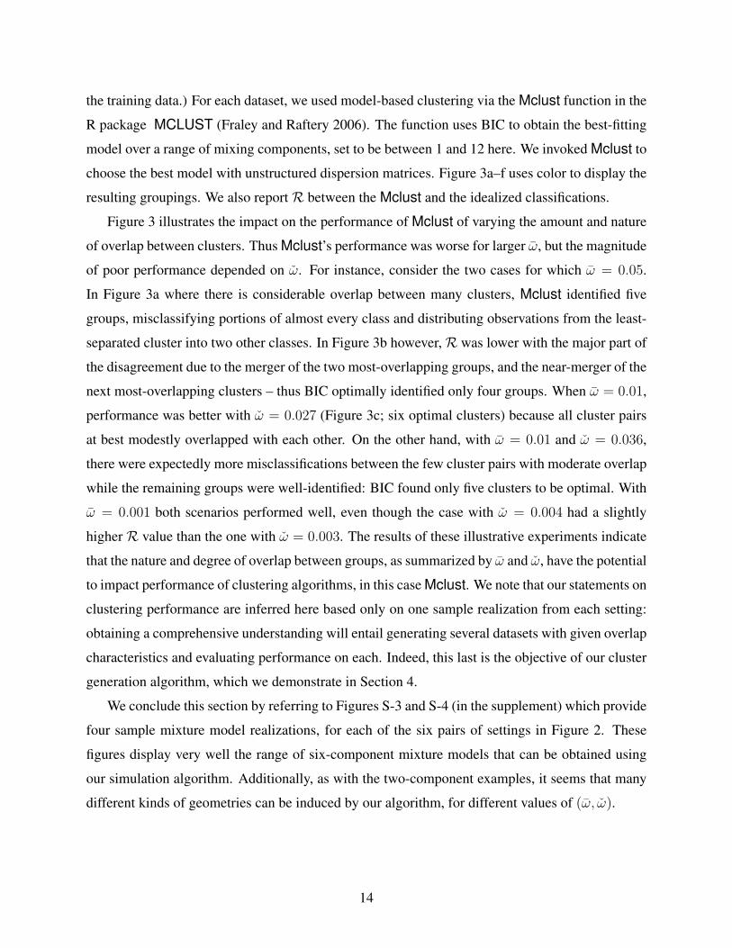
3.2 Simulation Experiments

0.0 0.2 0.4 0.6 0.8 1.0

0.0

0.2

0.4

0.6

0.8

1.0

Overlap

Adj

uste

d R

and

Inde

x

Figure 1: Mean ± SDs of Rs to evaluate cluster-

ing in two-component two-dimensional Gaussian

mixtures with different levels of overlap.

3.2.1. Validity of Overlap as Surrogate for

Clustering Complexity We first investigated

the validity of using our defined overlap as

a surrogate measure for clustering complex-

ity. We simulated 2,000 datasets, each with

100 observations, from a two-dimensional two-

component Gaussian mixture satisfying π∧ =

0.2 and a given overlap measure (since K = 2,

ω̄ = ω̌ ≡ ω). For each dataset, we applied the

EM algorithm (initialized, with the parameter

values that generated the dataset, to eliminate

possible ill-effects of improper initialization),

obtained parameter estimates, and computedRon the derived classification. This was done

for ω ∈ {0.001, 0.01, 0.02, 0.03, . . . , 1.0}. Fig-

ure 1 displays the mean and standard deviations

ofR for the different values of ω. Clearly, ω tracksR very well (inversely), providing support for

using our overlap measure as a reasonable surrogate for clustering complexity.

Figures S-1 and S-2 display sample two-component two-dimensional finite mixture models,

for ω ∈ [0.001, 0.75]. From these figures, it appears that distinctions between the two components

is sometimes unclear for ω = 0.15. The trend is accentuated at higher values: the two compo-

nents are visually virtually indistinguishable for ω > 0.5 or so and only the knowledge of their

11

being two Gaussian components perhaps provides us with some visual cue into their individual

structures. This matches the trend in Figure 1, since as components become indistinguishable, we

essentially move towards a random class assignment, for which caseR is constructed to have zero

expectation (Hubert and Arabie 1985). Based on Figure 1 and the realized mixtures in Figures S-1

and S-2, we conclude that pairwise overlaps of below 0.05 indicate well-separated components,

while those between around 0.05 and 0.1 indicate moderate separation. Pairwise overlaps above

0.15 in general produce poorly-separated components. We use this in determining possible choices

for ω̌ and ω̄. Figures S-1 and S-2 also provide some inkling into possible geometries induced by

our simulation algorithm for different ω.

3.2.2. Two-dimensional Experiments Figure 2 presents contour plots of sample two-dimensional

mixture distributions generated for K = 6 and different values (ω̄, ω̌). The choice of ω̌ was dic-

tated by ωσ = ω̄ and 2ω̄ and using the empirical β distribution for cluster overlaps discussed in

Section 2.2.2. We set π∧ = 0.14. Different choices of ω̄ and ω̌ provide us with realizations with

widely varying mixture (and cluster) characteristics. To see this, note that Figures 2a and 2b both

have high average overlap (ω̄ = 0.05) between cluster pairs. In Figure 2a, ω̌ is comparatively low,

which means that quite a few pairs of clusters have substantial overlap between them. In Figure 2b

however, the clusters are better-separated except for the top left cluster pair which is quite poorly-

separated, satisfying ω̌ and contributing substantially to the high ω̄ value of 0.05. Thus, in the first

case, many pairs of clusters have considerable overlap between them, but in the second case, a

few cluster pairs have substantial overlap while the rest overlap moderately. The same trends are

repeated for Figures 2c and 2d and Figures 2e and 2f, even though the cluster pairs are increasingly

better-separated, satisfying ω̄ = 0.01 and 0.001, respectively. Thus in Figure 2e, there is at best

modest overlap between any two clusters, while in Figure 2f, there is even less overlap, save for the

two clusters with smallest dispersions, which have far more overlap than the clusters in Figure 2e.

Impact on performance of MClust We also clustered a sample dataset obtained from each mix-

ture model in Figure 2. We generated 150 realizations from each distribution and classified each

observation to its most likely group, based on the true parameter values. The resulting classifica-

tion, displayed in each of Figures 3a–f via plotting character, represents the idealized grouping that

can perhaps ever be achieved at each point. (Note that even supervised learning in the form of QDA

may not always be expected to achieve this result, since the parameter values are estimated from

12

0.0

0.2

0.4

0.6

0.8

1.0

(a) ω̄ = 0.05, ω̌ = 0.135

0.0

0.2

0.4

0.6

0.8

1.0

(b) ω̄ = 0.05, ω̌ = 0.198

0.0

0.2

0.4

0.6

0.8

1.0

(c) ω̄ = 0.01, ω̌ = 0.027

0.0

0.2

0.4

0.6

0.8

1.0

(d) ω̄ = 0.01, ω̌ = 0.036

0.0

0.2

0.4

0.6

0.8

1.0

(e) ω̄ = 0.001, ω̌ = 0.0027

0.0

0.2

0.4

0.6

0.8

1.0

(f) ω̄ = 0.001, ω̌ = 0.0036

Figure 2: Contour plots of sample six-component mixture distributions in two dimensions obtained

using our algorithm and different settings of ω̄ and ω̌.

13

the training data.) For each dataset, we used model-based clustering via the Mclust function in the

R package MCLUST (Fraley and Raftery 2006). The function uses BIC to obtain the best-fitting

model over a range of mixing components, set to be between 1 and 12 here. We invoked Mclust to

choose the best model with unstructured dispersion matrices. Figure 3a–f uses color to display the

resulting groupings. We also reportR between the Mclust and the idealized classifications.

Figure 3 illustrates the impact on the performance of Mclust of varying the amount and nature

of overlap between clusters. Thus Mclust’s performance was worse for larger ω̄, but the magnitude

of poor performance depended on ω̌. For instance, consider the two cases for which ω̄ = 0.05.

In Figure 3a where there is considerable overlap between many clusters, Mclust identified five

groups, misclassifying portions of almost every class and distributing observations from the least-

separated cluster into two other classes. In Figure 3b however,R was lower with the major part of

the disagreement due to the merger of the two most-overlapping groups, and the near-merger of the

next most-overlapping clusters – thus BIC optimally identified only four groups. When ω̄ = 0.01,

performance was better with ω̌ = 0.027 (Figure 3c; six optimal clusters) because all cluster pairs

at best modestly overlapped with each other. On the other hand, with ω̄ = 0.01 and ω̌ = 0.036,

there were expectedly more misclassifications between the few cluster pairs with moderate overlap

while the remaining groups were well-identified: BIC found only five clusters to be optimal. With

ω̄ = 0.001 both scenarios performed well, even though the case with ω̌ = 0.004 had a slightly

higher R value than the one with ω̌ = 0.003. The results of these illustrative experiments indicate

that the nature and degree of overlap between groups, as summarized by ω̄ and ω̌, have the potential

to impact performance of clustering algorithms, in this case Mclust. We note that our statements on

clustering performance are inferred here based only on one sample realization from each setting:

obtaining a comprehensive understanding will entail generating several datasets with given overlap

characteristics and evaluating performance on each. Indeed, this last is the objective of our cluster

generation algorithm, which we demonstrate in Section 4.

We conclude this section by referring to Figures S-3 and S-4 (in the supplement) which provide

four sample mixture model realizations, for each of the six pairs of settings in Figure 2. These

figures display very well the range of six-component mixture models that can be obtained using

our simulation algorithm. Additionally, as with the two-component examples, it seems that many

different kinds of geometries can be induced by our algorithm, for different values of (ω̄, ω̌).

14

(a) K̂ = 5,R = 0.682 (b) K̂ = 4,R = 0.574

(c) K̂ = 6,R = 0.827 (d) K̂ = 5,R = 0.723

(e) K̂ = 6,R = 0.964 (f) K̂ = 6,R = 0.968

Figure 3: Groupings obtained using Mclust on a realization from the corresponding mixture dis-

tributions of Figure 2. Color indicates the Mclust grouping and character the best possible classi-

fication with known parameter values. Optimal numbers of clusters as determined by BIC are also

noted in the captions for each sub-figure.

15

3.2.3. Higher-dimensional Examples We have also successfully used our algorithm to simulate

mixture distributions of up to 50 components and for dimensions of up to 100. Note that in terms

of computational effort, our algorithm is quadratic in the number of clusters because we calculate

all pairwise overlaps between components. There is no ready technique for displaying higher-

dimensional distributions, so we introduce the parallel distribution plot, and use this in Figure 4 to

illustrate some sample mixture distributions realized using our algorithm.

Parallel distribution plot The objective of the parallel distribution plot is to display a mul-

tivariate mixture distribution in a way that contrasts and highlights the distinctiveness of each

mixture component. We note that the dispersion matrix of a mixture density of the kind consid-

ered in this paper, i.e. g(x) =K∑k=1

πkφ(x;µk,Σk), is given by Σ• =K∑k=1

πkΣk +K∑k=1

πkµkµ′k −

K∑l=1

K∑k=1

πlπkµlµ′k. Let V • be the matrix of orthonormal eigenvectors [v1

...v2... . . .

...vp], correspond-

ing to the eigenvalues d1 ≥ d2 ≥ . . . dp of Σ•. Applying the rotation V ′• to the mixture pro-

vides us with the principal components (PCs) of the mixture. These PCs are uncorrelated with

decreasing variance given by d1 ≥ d2 ≥ . . . dp. Also, the distribution of these PCs is still a

mixture, of (rotated) Gaussians, with the kth rotated component having mixing proportion πk

and multivariate Gaussian distribution with mean vector V ′•µk and dispersion V ′•ΣkV •. We

display the distribution of each mixture component, borrowing ideas from parallel coordinate

plots (Inselberg 1985; Wegman 1990). Note that each component k only contributes a total mass

of probability πk. For each component k and jth marginal distribution (in projection space), locate

the quantiles {qkj1, qkj2, . . . , qkjm} corresponding to the m− 1 equal increments in probabilities in

(0, πk). The quantile qkji of the jth marginal distribution is connected to the quantile qk(j+1)i of the

(j + 1)th marginal distribution by means of a parallel coordinate plot. The polygon formed by the

two successive quantiles and the lines joining each is shaded with a given color, unique to every

cluster component, and with varying opacity. The opacity at the vertical edges of each polygon

is proportional to the density at the mid-point of the interval (qkji, qkj(i+1)). Inside the polygon,

the opacity varies smoothly in the horizontal direction (only) as a convex combination of the edge

opacities. Thus, we get a parallel distribution plot. Finally, we contend that though we develop and

use parallel distribution plots here solely to display mixture distributions, they can also be used to

display grouped data, by replacing each theoretical quantile by its empirical cousin.

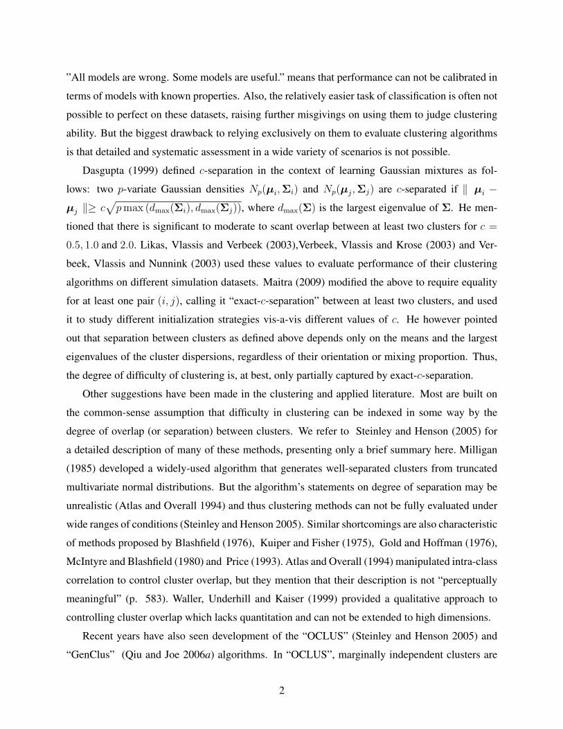
Figure 4 displays parallel distribution plots of sample six-component five-dimensional mixture

16

1 2 3 4 5

(a) ω̄ = 0.05, ω̌ = 0.135

1 2 3 4 5

(b) ω̄ = 0.05, ω̌ = 0.198

1 2 3 4 5

(c) ω̄ = 0.001, ω̌ = 0.003

1 2 3 4 5

(d) ω̄ = 0.001, ω̌ = 0.004

Figure 4: Parallel distribution plots of six-component mixture distributions in five dimensions and

different settings of ω̄ and ω̌.

17

distributions obtained using our algorithm at four different settings. As expected, the total spread

of the mixture distribution decreases with increase in PC dimension. The mixture components are

also more separable in the first few PCs than in the later ones. This is because the dominant source

of variability in the mixture distribution is between-cluster variability and that is better separated

in the first few components. Towards the end, the PCs are dominated by random noise arising

from the within-cluster variability over the between-cluster variability. Figure 4a illustrates the

case for when ω̄ = 0.05 and ω̌ = 0.135, while Figure 4b illustrates the case for when ω̄ = 0.05

and ω̌ = 0.198. In both cases, there is overlap between several clusters, but in the second case,

the overlap between the green and red components dominates. In both cases, between-cluster

variability is dominated by its within-cluster cousin fairly soon among the PCs. On the other hand,

Figure 4c and 4d indicate that between-cluster variability continues to dominate within-cluster

variability even for higher PCs. Also, the mixture components are much better separated on the

whole for Figure 4c and 4d than for Figure 4a and 4b, but the blue and cyan clusters dominate the

average overlap in Figure 4d.

3.2.4. Other Properties of Simulation Algorithm We also explored variability in simulated mix-

ture distributions in higher dimensions. We generated 25 datasets each, for different combinations

of (ω̄, ω̌) from 7-, 9- and 11-component multivariate normal mixtures in 5-, 7- and 10-dimensional

spaces, respectively. For every p, we set ω̄ to be 0.05, 0.01 and ω̌ to be such that the empirical coef-

ficient of variation (ωσ/ω̄) in overlap between components was 1 and 2. π∧s were stipulated to be

0.06, 0.04 and 0.03 for the 5-, 7- and 10-dimensional experiments, respectively, so that there would

be at least p+ 1 observations from each of the 7, 9 and 11 components with very high probability,

when we drew samples of size n = 500, 1,000, and 1, 500, respectively, in further experiments in

Section 4.) Expected Kullback-Leibler divergences calculated for each pair of mixture model den-

sities obtained for each setting, and detailed in Table S-1 (supplement), show substantial variability

in simulated models.

We also analyzed the number of times initial realizations had to be discarded and regenerated

in order to guarantee Step 3 of the algorithm in Section 2.2.1 or Step 2 of the algorithm in Sec-

tion 2.2.2 in the generation of these sets of mixture models. The results are reported in Table S-2 in

the supplement. As expected, there is a large number of regenerations needed for larger numbers

of clusters and when the average overlap is closer to the maximum overlap. We note, however,

that these regenerations are at the trial stage of each algorithm, with evaluations and regenerations

18

done in each case before the iterative stage is entered into.

4. UTILITY OF PROPOSED ALGORITHM

Here we demonstrate utility of the proposed algorithm in evaluating some initialization methods

for Gaussian finite mixture modeling and model-based clustering algorithms. Initialization is cru-

cially important in the performance of many iterative optimization-partitioning algorithms with a

number of largely heuristic approaches in the literature. We evaluate four initialization methods

that have previously shown promise in model-based clustering. Our objective is to illustrate the

utility of our algorithm in comparing and contrasting performance under different scenarios and

see if recommendations, if any, can be made with regard to each method.

Our first initialization approach was the em-EM algorithm of Biernacki, Celeux and Govaert

(2003), so named because it uses several short runs of the EM, each initialized with a valid (in

terms of existence of likelihood) random start as parameter estimates. Each short run stops the

EM algorithm, initialized with the above random start, according to a lax convergence criterion.

The procedure is repeated until an overall pre-specified number of total short run iterations is ex-

hausted. At this point, the solution with the highest log likelihood value is declared to be the

initializer for the long EM, which then proceeds to termination using the desired stringent conver-

gence criterion. We used p2 total short run iterations and a lax convergence criterion of no more

than one percent relative change in log likelihood for our experiments. Our second approach, the

Rnd-EM, used Maitra (2009)’s proposed modification that eliminates each short EM step by just

evaluating the likelihood at the initial valid random start and choosing the parameters with highest

likelihood. With the short em run eliminated, the best initializer is thus obtained from a number

of candidate points equivalent to the total number (p2) of short run iterations. Our third approach

used Mclust which integrates model-based hierarchical clustering with a likelihood gain merge

criterion to determine an initial grouping (Fraley and Raftery 2006) from where initializing param-

eter estimates are fed into the EM algorithm. Finally, we used the multi-staged approach proposed

by Maitra (2009) in providing initial values for the EM algorithm. This is a general strategy pro-

posed by him to find a large number of local modes, and to choose representatives from theK most

widely-separated ones. We use the specific implementation of this algorithm in Maitra (2009).

Our demonstration suite used simulated datasets generated from the mixture models in Sec-

tion 3.2.4. In this utility demonstrator, we assumed thatK was known in all cases. We calculatedRfor each derived classification relative to the grouping obtained by classifying the datasets with EM

19

initialized with the true parameter values. In each case, we also evaluated estimation performance

of these converged EM results by calculating the expected Kullback-Leibler divergence (KL) of

the estimated model relative to the true mixture model.

Table 2 summarizes results for the 5- and 10-dimensional experiments. Results for the 7-

dimensional experiments are provided in Table S-3. It is clear that Mclust outperforms the other

algorithms for cases with small average overlap. In general, it also does better than emEM or Rnd-

EM when the variation in overlap between clusters is higher. Further, there is some degradation

in Mclust’s performance with increasing dimensionality. On the other hand, emEM and Rnd-EM

do not appear to be very different from each other: the latter seems to perform better with higher

dimensions. This may be because higher dimensions mean a larger number of short run iterations

(for emEM) and random starts (for Rnd-EM) in our setup. This suggests that using computing

power to evaluate more potential starting points may be more profitable than using it to running

short run iterations. It is significant to note, however that both emEM and Rnd-EM are outclassed

by Mclust in all cases when cluster pairs have low average overlap. We note that the multi-staged

approach of Maitra (2009) very rarely ourperforms the others. This is a surprising finding in that it

contradicts the findings in Maitra (2009) where performance was calibrated on simulation exper-

iments indexed using exact-c-separation. Finally, we note that while there is not much difference

between performance in clustering and maximum likelihood parameter estimation in mixture mod-

els, with both R and KL having very similar trends, they are not completely identical. This is a

pointer to the fact that what may be the perfect sauce for the goose (parameter estimation in finite

mixture models) may not be perfect for the gander (model-based clustering) and vice-versa.

The above is a demonstration of the benchmarking that can be made possible using our cluster

simulation algorithm. We note that Mclust is the best performer when clusters are well-separated

and Rnd-EM and emEM as a better performer when clusters are less well-separated. Note that

Rnd-EM and emEM perform similar and often split honors in many cases. There is thus, not much

distinction between these two methods, even though Rnd-EM seems to be better at more efficient

use of computing resources. Thus, Mclust may be used when clusters are a priori known to be

well-separated. When clusters are known to be poorly-separated, Rnd-EM may be used. Otherwise,

if separation between clusters is not known, a better option may be to try out Rnd-EM and Mclust

and choose the one with the highest observed log likelihood.

20

Table 2: Adjusted Rand (R) similarity measures of EM-cluster groupings and expected Kullback-

Leibler divergences (KL) of estimated mixture model densities obtained, using different initializa-

tion strategies (starts), over 25 replications for different overlap characteristics. Summary statistics

represented are the medianR (R 12) and median KL (KL 1

2) and corresponding interquartile ranges

(IR12

and IKL12

). Finally, R#1 and KL#1 represent the number of replications (out of 25) for which

the given initialization strategy did as well (in terms of higherR and lowerKL) as the best strategy.

Star

ts p = 5, k = 7, n = 500 p = 10, k = 11, n = 1, 500

ω̄ 0.15 0.10 0.05 0.01 0.001 0.15 0.10 0.05 0.01 0.001

ω̌ 0.49 0.319 0.15 0.27 0.03 0.05 0.003 0.005 0.62 0.41 0.20 0.44 0.04 0.08 0.004 0.008

emE

M

R 12

0.35 0.45 0.69 0.67 0.79 0.81 0.89 0.88 0.25 0.34 0.57 0.55 0.84 0.86 0.87 0.92

IR12

0.13 0.15 0.15 0.14 0.19 0.14 0.16 0.20 0.18 0.15 0.08 0.08 0.07 0.10 0.12 0.07

R#1 6 7 10 7 5 2 6 3 13 11 13 9 8 10 2 0

KL 12

0.30 0.30 0.32 0.28 0.29 0.29 0.34 0.30 0.46 0.49 0.48 0.49 0.52 0.47 0.47 0.50

IKL12

0.05 0.08 0.05 0.07 0.17 0.11 0.09 0.14 0.05 0.07 0.05 0.07 0.09 0.08 0.14 0.12

KL#1 10 9 11 10 6 5 1 1 10 10 14 11 5 7 0 1

Rnd

-EM

R 12

0.37 0.46 0.64 0.61 0.84 0.83 0.89 0.91 0.23 0.31 0.58 0.58 0.83 0.78 0.91 0.92

IR12

0.18 0.12 0.12 0.18 0.16 0.13 0.17 0.13 0.11 0.19 0.15 0.11 0.11 0.11 0.14 0.12

R#1 13 8 6 10 5 2 3 6 6 11 11 12 8 0 1 0

KL 12

0.30 0.29 0.32 0.30 0.28 0.29 0.33 0.34 0.47 0.50 0.50 0.49 0.47 0.46 0.48 0.46

IKL12

0.07 0.04 0.07 0.09 0.10 0.05 0.19 0.07 0.05 0.06 0.05 0.06 0.09 0.07 0.07 0.14

KL#1 14 9 9 7 3 3 5 4 7 12 8 10 11 4 2 1

Mcl

ust

R 12

0.28 0.40 0.65 0.62 0.95 0.96 1.0 1.0 0.16 0.25 0.45 0.48 0.83 0.84 1.0 1.0

IR12

0.16 0.13 0.19 0.14 0.14 0.15 0.00 0.01 0.16 0.21 0.16 0.20 0.09 0.10 0.01 0.00

R#1 5 6 9 6 15 19 23 20 5 2 0 3 9 12 22 25

KL 12

0.35 0.33 0.35 0.32 0.22 0.24 0.18 0.19 0.50 0.58 0.55 0.55 0.47 0.42 0.33 0.31

IKL12

0.08 0.08 0.05 0.07 0.10 0.07 0.04 0.05 0.09 0.09 0.12 0.06 0.07 0.10 0.08 0.05

KL#1 0 2 4 6 15 17 17 13 5 2 2 3 8 13 23 23

Mul

ti-st

aged

R 12

0.22 0.40 0.50 0.52 0.68 0.70 0.86 0.91 0.05 0.12 0.36 0.42 0.64 0.70 0.78 0.78

IR12

0.17 0.24 0.21 0.16 0.24 0.17 0.22 0.20 0.12 0.18 0.22 0.33 0.16 0.20 0.14 0.17

R#1 1 4 0 2 0 2 1 5 1 1 1 1 0 3 0 0

KL 12

0.35 0.32 0.42 0.36 0.42 0.41 0.35 0.30 0.56 0.58 0.65 0.58 0.63 0.62 0.77 0.73

IKL12

0.16 0.09 0.23 0.12 0.20 0.17 0.34 0.22 0.85 0.08 0.17 0.21 0.12 0.20 0.43 0.28

KL#1 1 5 1 2 1 0 2 7 3 1 1 1 1 1 0 0

21

5. DISCUSSION

In this paper, we develop methodology and provide an algorithm for generating clustered data

according to desired cluster overlap characteristics. Such characteristics serve as a surrogate for

clustering difficulty and can lead to better understanding and calibration of the performance of

clustering algorithms. Our algorithm generates clusters according to exactly pre-specified average

and maximal pairwise overlap. We illustrate our algorithm in the context of mixture distributions

and in sample two- and five-dimensional experiments with six components. We also introduce

the parallel distribution plot to display mixture distributions in high dimensions. A R package

implementing the algorithm has been developed and will be publicly released soon. Finally, we

demonstrate potential utility of the algorithm in a test scenario where we evaluate performance of

four initialization strategies in the context of EM-clustering in a range of clustering settings over

several dimensions and numbers of true groups. This ability to study properties of different clus-

tering algorithms and related strategies is the main goal for devising our suggested methodology.

One reviewer has asked why we define pairwise overlap in terms of the unweighted sum

ωi|j + ωj|i, rather than the weighted sum (πjωi|j + πiωj|i)/(πi + πj). We preferred the former

because weighting would potentially damp out the effect of misclassification of components with

small relative mixing proportions, even though they affect clustering performance (as indexed by

R). We have not investigated using the weighted sum as an overlap measure: it would be interest-

ing to study its performance. We note however, that Figure 1 indicates thatR is very well-tracked

by our defined overlap measure. Also, our algorithm was developed in the context of soft clus-

tering using Gaussian mixture models. However, the methodology developed here can be very

easily applied to the case of hard clustering with a fixed partition Gaussian clustering model. A

third issue not particularly emphasized in this paper is that Theorem 2.1 can help summarize the

distinctiveness between groups obtained by Gaussian clustering of a given dataset. Thus, clustered

data can be analyzed to study how different one cluster is from another by measuring the overlap

between them. As mentioned in Section 2.2.3, desired scatter can also be very easily incorpo-

rated in our algorithm. In this paper, we characterize cluster overlap in terms of the average and

maximum pairwise overlap. It would be interesting to see if summaries based on other proper-

ties of overlap could also be developed in a practical setting. Finally, our algorithm is specific to

generating Gaussian mixtures with desired cluster overlap properties and can not readily handle

heavy-tailed or skewed distributions. One possibility may be to use the Box-Cox transformation

in each dimension to match desired skewness and (approximately) desired overlap characteristics.

22

Thus, while the methodology suggested in this paper can be regarded as an important contribution

to for evaluating clustering algorithms, quite a few issues meriting further attention remain.

ACKNOWLEDGMENTS

We thank the editor, an associate editor and two referees whose helpful suggestions and insightful

comments greatly improved the quality of this manuscrpt.

SUPPLEMENTARY MATERIALS

Additional Investigations: Sections S-1–3 along with Figures S-1–4 and Tables S-1–3 are in the

supplementary materials archive of the journal website. (appendix.pdf)

R-package: R-package ”MixSim” implementing this algorithm is available on C-RAN. (MixSim 0.1-

04.tar.gz)

REFERENCESAnderson, E. (1935), “The Irises of the Gaspe Peninsula,” Bulletin of the American Iris Society,

59, 2–5.

Atlas, R., and Overall, J. (1994), “Comparative evaluation of two superior stopping rules for hier-archical cluster analysis,” Psychometrika, 59, 581–591.

Bartlett, M. S. (1939), “A note on tests of significance in multivariate analysis,” Proceedings of theCambridge Philosophical Society, 35, 180–185.

Biernacki, C., Celeux, G., and Govaert, G. (2003), “Choosing starting values for the EM algorithmfor getting the highest likelihood in multivariate Gaussian mixture models,” ComputationalStatistics and Data Analysis, 413, 561–575.

Blashfield, R. K. (1976), “Mixture model tests of cluster analysis - Accuracy of 4 agglomerativehierarchical methods,” Psychological Bulletin, 83, 377–388.

Box, G. E. P., and Draper, N. R. (1987), Empirical Model-Building and Response Surfaces, NewYork, NY: John Wiley.

Brodatz, P. (1966), A Photographic Album for Artists and Designers, New York: Dover.

Campbell, N. A., and Mahon, R. J. (1974), “A Multivariate Study of Variation in Two Species ofRock Crab of Genus Leptograsus,” Australian Journal of Zoology, 22, 417–25.

Dasgupta, S. (1999), Learning mixtures of Gaussians,, in Proc. IEEE Symposium on Foundationsof Computer Science, New York, pp. 633–644.

23

Davies, R. (1980), “The distribution of a linear combination of χ2 random variables,” AppliedStatistics, 29, 323–333.

D.J. Newman, S. Hettich, C. B., and Merz, C. (1998), “UCI Repository of machine learningdatabases,” , .URL: http://www.ics.uci.edu/∼mlearn/MLRepository.html

Everitt, B. S., Landau, S., and Leesem, M. (2001), Cluster Analysis (4th ed.), New York: HodderArnold.

Forina, M. (1991), PARVUS - An extendible package for data exploration, classification and cor-relation., Genoa, Italy: Institute of Pharmaceutical and Food Analysis and Technologies.

Forsythe, G., Malcolm, M., and Moler, C. (1980), Computer methods for mathematical computa-tions, Moscow: Mir.

Fraley, C., and Raftery, A. E. (2002), “Model-Based Clustering, Discriminant Analysis, and Den-sity Estimation,” Journal of the American Statistical Association, 97, 611–631.

Fraley, C., and Raftery, A. E. (2006), MCLUST Version 3 for R: Normal Mixture Modeling andModel-Based Clustering,, Technical Report 504, University of Washington, Department ofStatistics, Seattle, WA. 2006.

Gold, E. M., and Hoffman, P. J. (1976), “Flange detection cluster analysis,” Multivariate Behav-ioral Research, 11, 217–235.

Hartigan, J. (1985), “Statistical theory in clustering,” Journal of Classification, 2, 63–76.

Hubert, L., and Arabie, P. (1985), “Comparing partitions,” Journal of Classification, 2, 193–218.

Inselberg, A. (1985), “The plane with parallel coordinates,” The Visual Computer, 1, 69–91.

Kaufman, L., and Rousseuw, P. J. (1990), Finding Groups in Data, New York: John Wiley andSons, Inc.

Kettenring, J. R. (2006), “The practice of cluster analysis,” Journal of classification, 23, 3–30.

Kuiper, F. K., and Fisher, L. (1975), “A Monte Carlo comparison of six clustering procedures,”Biometrics, 31, 777–783.

Likas, A., Vlassis, N., and Verbeek, J. J. (2003), “The global k-means clustering algorithm,” Pat-tern Recognition, 36, 451–461.

Maitra, R. (2009), “Initializing Partition-Optimization Algorithms,” IEEE/ACM Transactions onComputational Biology and Bioinformatics, 6, 144–157.

Maitra, R., and Ramler, I. P. (2008), “Clustering in the Presence of Scatter,” Biometrics, Z, XXX–YYY.

24

McIntyre, R. M., and Blashfield, R. K. (1980), “A nearest-centroid technique for evaluating theminimum-variance clustering procedure,” Multivariate Behavioral Research, 15, 225–238.

McLachlan, G. J., and Basford, K. E. (1988), Mixture Models: Inference and Applications toClustering, New York: Marcel Dekker.

Milligan, G. W. (1985), “An algorithm for generating artificial test clusters,” Psychometrika,50, 123–127.

Murtagh, F. (1985), Multi-dimensional clustering algorithms, Berlin; New York: Springer-Verlag.

Nakai, K., and Kinehasa, M. (1991), “Expert sytem for predicting protein localization sites ingram-negative bacteria,” PROTEINS: Structure, Function, and Genetics, 11, 95–110.

Press, S. J. (1966), “Linear combinations of non-central chi-square variates,” Annals of Mathemat-ical Statistics, 37, 480–487.

Price, L. J. (1993), “Identifying cluster overlap with normix population membership probabilities,”Multivariate Behavioral Research, 28, 235–262.

Qiu, W., and Joe, H. (2006a), “Generation of random clusters with specified degree of separation,”Journal of Classification, 23, 315–334.

Qiu, W., and Joe, H. (2006b), “Separation index and partial membership for clustering,” Compu-tational Statistics and Data Analysis, 50, 585–603.

Ramey, D. B. (1985), “Nonparametric clustering techniques,” in Encyclopedia of Statistical Sci-ence, Vol. 6, New York: Wiley, pp. 318–319.

Ruspini, E. (1970), “Numerical methods for fuzzy clustering,” Information Science, 2, 319–350.

Slater, L. J. (1960), Confluent hypergeometric functions, London: Cambridge University Press.

Steinley, D., and Henson, R. (2005), “OCLUS: An Analytic Method for Generating Clusters withKnown Overlap,” Journal of Classification, 22, 221–250.

Tseng, G. C., and Wong, W. H. (2005), “Tight clustering: A resampling-based approach for iden-tifying stable and tight patterns in data,” Biometrics, 61, 10–16.

Verbeek, J., Vlassis, N., and Krose, B. (2003), “Efficient greedy learning of Gaussian mixturemodels,” Neural Computation, 15, 469–485.

Verbeek, J., Vlassis, N., and Nunnink, J. (2003), “A variational EM algorithm for large-scalemixture modeling,” Annual Conference of the Advanced School for Computing and Imaging,pp. 1–7.

Waller, N. G., Underhill, J. M., and Kaiser, H. A. (1999), “A method for generating simulated plas-modes and artificial test clusters with user-defined shape, size, and orientation,” MultivariateBehavioral Research, 34, 123–142.

25

Wegman, E. (1990), “Hyperdimensional data analysis using parallel coordinates,” Journal of theAmerican Statistical Association, 85, 664–675.

26