Embed Size (px)
Citation preview

Yien Fuang TiongHasan Jehanzaib
Yaseen BokhamseenFei Zhao
Zalani KamarudinKarthik Surisetty
Reservoir Characterisation Study
Group A
15/04/2023 2
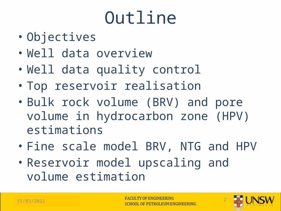
Outline• Objectives• Well data overview• Well data quality control• Top reservoir realisation• Bulk rock volume (BRV) and pore volume in
hydrocarbon zone (HPV) estimations• Fine scale model BRV, NTG and HPV• Reservoir model upscaling and volume
estimation
15/04/2023 3
Objectives
• Using stochastic simulation, construct reservoir model from well data
• Volume estimation• Investigate the accuracy of upscaling via
volume comparison

15/04/2023 4
Well locationsWell locations
X Location
Y L
ocat
ion
20 40 60 80 100 120 140 160 180 200
20
40
60
80
100
120
140
160
180
200
No well data in the circled areas!
14 exploration wells were drilled
15/04/2023 5
Comments regarding wells
• Well data covers a wide area of reservoir, especially in the east and south-west
• Lacking data in north-west and left centre of the reservoir
• Affects reliability of reservoir model at those areas
• All wells intersect oil-water contact and bottom of the reservoir. All contacts are shallower than reservoir bottom
15/04/2023 6
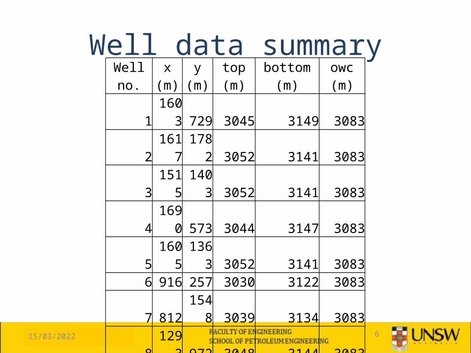
Well data summaryWell no. x (m) y (m) top (m) bottom (m) owc (m)
1 1603 729 3045 3149 30832 1617 1782 3052 3141 30833 1515 1403 3052 3141 30834 1690 573 3044 3147 30835 1605 1363 3052 3141 30836 916 257 3030 3122 30837 812 1548 3039 3134 30838 1293 972 3048 3144 30839 540 567 3007 3095 3083
10 238 660 2974 3085 308311 1770 1608 3052 3141 308312 1211 645 3043 3147 308313 1226 1663 3050 3140 308314 1441 1302 3052 3141 3083

15/04/2023 7
Well Data Quality Control
• Only well data is provided for stochastic simulation
• Important to conduct quality check• For properties like porosity and permeability,
check for trends in x and y directions• Check quality of data
15/04/2023 8
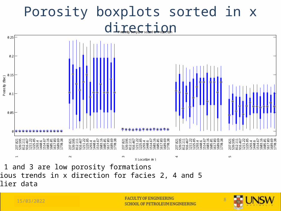
Porosity boxplots sorted in x direction
0
0.05
0.1
0.15
0.2
0.25
1 2 3 4 5
237.
821
539.
595
812.
111
916.
467
1211
.22
1225
.85
1293
.414
40.6
1514
.67
1603
.16
1605
.01
1617
.03
1689
.69
1770
.38
237.
821
539.
595
812.
111
916.
467
1211
.22
1225
.85
1293
.414
40.6
1514
.67
1603
.16
1605
.01
1617
.03
1689
.69
1770
.38
237.
821
539.
595
812.
111
916.
467
1211
.22
1225
.85
1293
.414
40.6
1514
.67
1603
.16
1605
.01
1617
.03
1689
.69
1770
.38
237.
821
539.
595
812.
111
916.
467
1211
.22
1225
.85
1293
.414
40.6
1514
.67
1603
.16
1605
.01
1617
.03
1689
.69
1770
.38
237.
821
539.
595
812.
111
916.
467
1211
.22
1225
.85
1293
.414
40.6
1514
.67
1603
.16
1605
.01
1617
.03
1689
.69
1770
.38
X Location (m)
Por
osity
(fr
ac)
Porosity boxplots sorted in X direction
• Facies 1 and 3 are low porosity formations• No obvious trends in x direction for facies 2, 4 and 5• No outlier data
15/04/2023 9
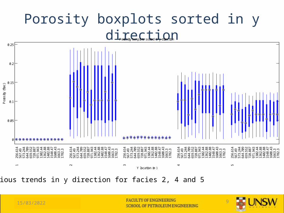
Porosity boxplots sorted in y direction
0
0.05
0.1
0.15
0.2
0.25
1 2 3 4 5
256.
614
567.
4957
3.24
464
4.70
965
9.55
272
8.88
797
1.94
313
02.4
413
62.8
814
02.8
815
48.4
716
08.4
316
63.3
1782
.3
256.
614
567.
4957
3.24
464
4.70
965
9.55
272
8.88
797
1.94
313
02.4
413
62.8
814
02.8
815
48.4
716
08.4
316
63.3
1782
.3
256.
614
567.
4957
3.24
464
4.70
965
9.55
272
8.88
797
1.94
313
02.4
413
62.8
814
02.8
815
48.4
716
08.4
316
63.3
1782
.3
256.
614
567.
4957
3.24
464
4.70
965
9.55
272
8.88
797
1.94
313
02.4
413
62.8
814
02.8
815
48.4
716
08.4
316
63.3
1782
.3
256.
614
567.
4957
3.24
464
4.70
965
9.55
272
8.88
797
1.94
313
02.4
413
62.8
814
02.8
815
48.4
716
08.4
316
63.3
1782
.3
Y location (m)
Porosity boxplots sorted in y direction
Por
osity
(fr
ac)
• No obvious trends in y direction for facies 2, 4 and 5
15/04/2023 10
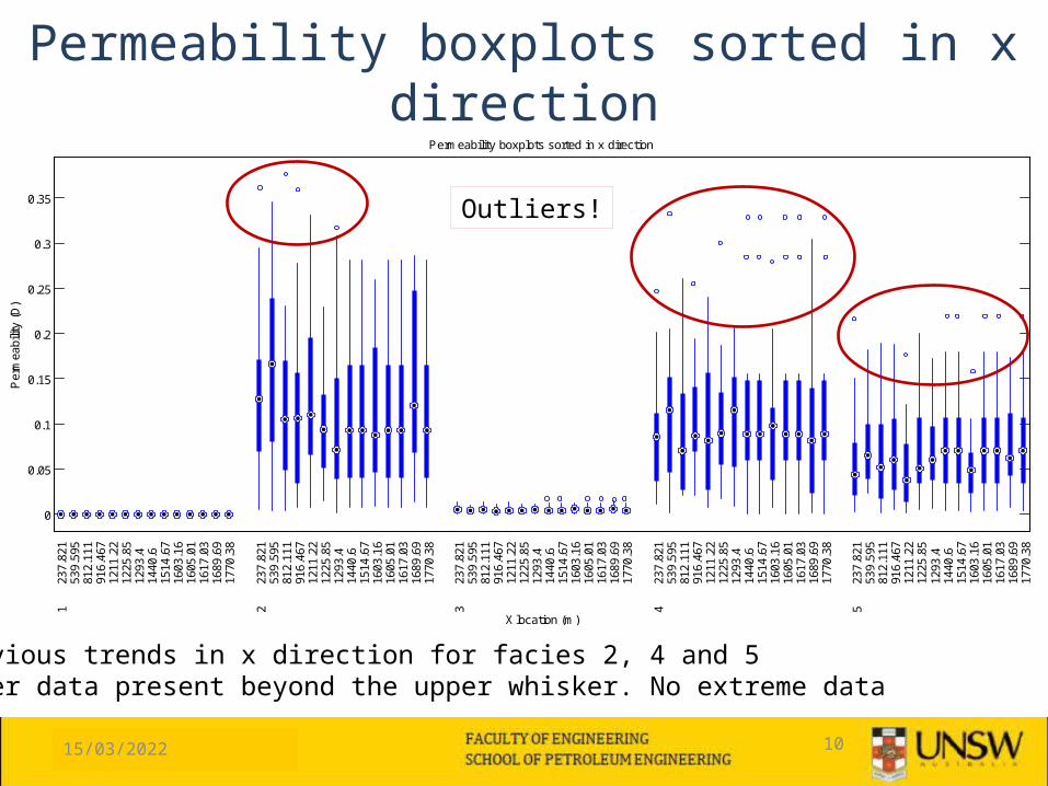
Permeability boxplots sorted in x direction
0
0.05
0.1
0.15
0.2
0.25
0.3
0.35
1 2 3 4 5
237.
821
539.
595
812.
111
916.
467
1211
.22
1225
.85
1293
.414
40.6
1514
.67
1603
.16
1605
.01
1617
.03
1689
.69
1770
.38
237.
821
539.
595
812.
111
916.
467
1211
.22
1225
.85
1293
.414
40.6
1514
.67
1603
.16
1605
.01
1617
.03
1689
.69
1770
.38
237.
821
539.
595
812.
111
916.
467
1211
.22
1225
.85
1293
.414
40.6
1514
.67
1603
.16
1605
.01
1617
.03
1689
.69
1770
.38
237.
821
539.
595
812.
111
916.
467
1211
.22
1225
.85
1293
.414
40.6
1514
.67
1603
.16
1605
.01
1617
.03
1689
.69
1770
.38
237.
821
539.
595
812.
111
916.
467
1211
.22
1225
.85
1293
.414
40.6
1514
.67
1603
.16
1605
.01
1617
.03
1689
.69
1770
.38
X location (m)
Per
mea
bilit
y (D
)
Permeability boxplots sorted in x direction
• No obvious trends in x direction for facies 2, 4 and 5• Outlier data present beyond the upper whisker. No extreme data
Outliers!
15/04/2023 11
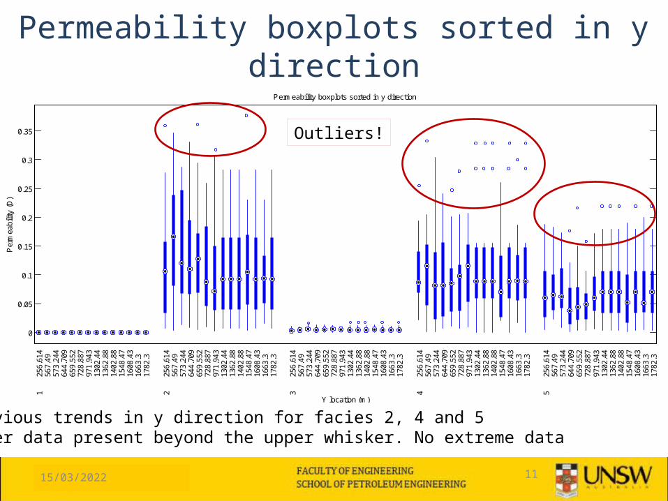
Permeability boxplots sorted in y direction
0
0.05
0.1
0.15
0.2
0.25
0.3
0.35
1 2 3 4 5
256.
614
567.
4957
3.24
464
4.70
965
9.55
272
8.88
797
1.94
313
02.4
413
62.8
814
02.8
815
48.4
716
08.4
316
63.3
1782
.3
256.
614
567.
4957
3.24
464
4.70
965
9.55
272
8.88
797
1.94
313
02.4
413
62.8
814
02.8
815
48.4
716
08.4
316
63.3
1782
.3
256.
614
567.
4957
3.24
464
4.70
965
9.55
272
8.88
797
1.94
313
02.4
413
62.8
814
02.8
815
48.4
716
08.4
316
63.3
1782
.3
256.
614
567.
4957
3.24
464
4.70
965
9.55
272
8.88
797
1.94
313
02.4
413
62.8
814
02.8
815
48.4
716
08.4
316
63.3
1782
.3
256.
614
567.
4957
3.24
464
4.70
965
9.55
272
8.88
797
1.94
313
02.4
413
62.8
814
02.8
815
48.4
716
08.4
316
63.3
1782
.3
Y location (m)
Per
mea
bilit
y (D
)
Permeability boxplots sorted in y direction
• No obvious trends in y direction for facies 2, 4 and 5• Outlier data present beyond the upper whisker. No extreme data
Outliers!

15/04/2023 12
Question to Ask?
• Is the permeability outlier data dubious?• Conduct further quality check to find out
15/04/2023 13
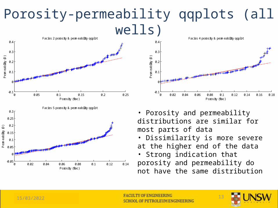
Porosity-permeability qqplots (all wells)
0 0.05 0.1 0.15 0.2 0.25-0.1
0
0.1
0.2
0.3
0.4
Porosity (frac)
Per
mea
bilit
y (D
)
Facies 2 porosity & permeability qqplot
0 0.02 0.04 0.06 0.08 0.1 0.12 0.14 0.16 0.18-0.1
0
0.1
0.2
0.3
0.4
Porosity (frac)
Per
mea
bilit
y (D
)
Facies 4 porosity & permeability qqplot
0 0.02 0.04 0.06 0.08 0.1 0.12 0.14-0.05
0
0.05
0.1
0.15
0.2
0.25
0.3
Porosity (frac)
Per
mea
bilit
y (D
)
Facies 5 porosity & permeability qqplot
• Porosity and permeability distributions are similar for most parts of data• Dissimilarity is more severe at the higher end of the data• Strong indication that porosity and permeability do not have the same distribution
15/04/2023 14
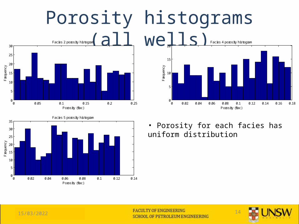
Porosity histograms (all wells)
0 0.05 0.1 0.15 0.2 0.250
5
10
15
20
25
30
Porosity (frac)
Fre
quen
cy
Facies 2 porosity histogram
0 0.02 0.04 0.06 0.08 0.1 0.12 0.14 0.16 0.180
5
10
15
20
Porosity (frac)
Fre
quen
cy
Facies 4 porosity histogram
0 0.02 0.04 0.06 0.08 0.1 0.12 0.140
5
10
15
20
25
30
35Facies 5 porosity histogram
Porosity (frac)
Fre
quen
cy
• Porosity for each facies has uniform distribution
15/04/2023 15
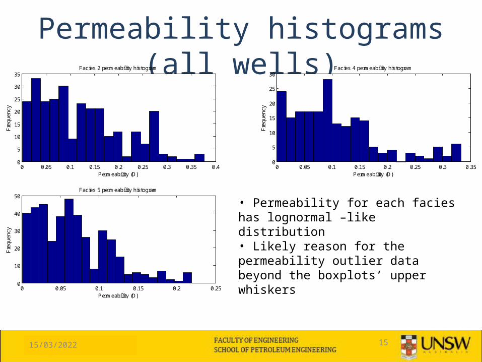
Permeability histograms (all wells)
0 0.05 0.1 0.15 0.2 0.25 0.3 0.35 0.40
5
10
15
20
25
30
35Facies 2 permeability histogram
Permeability (D)
Fre
quen
cy
0 0.05 0.1 0.15 0.2 0.25 0.3 0.350
5
10
15
20
25
30
Permeability (D)
Fre
quen
cy
Facies 4 permeability histogram
0 0.05 0.1 0.15 0.2 0.250
10
20
30
40
50
Permeability (D)
Fre
quen
cy
Facies 5 permeability histogram
• Permeability for each facies has lognormal –like distribution• Likely reason for the permeability outlier data beyond the boxplots’ upper whiskers
15/04/2023 16
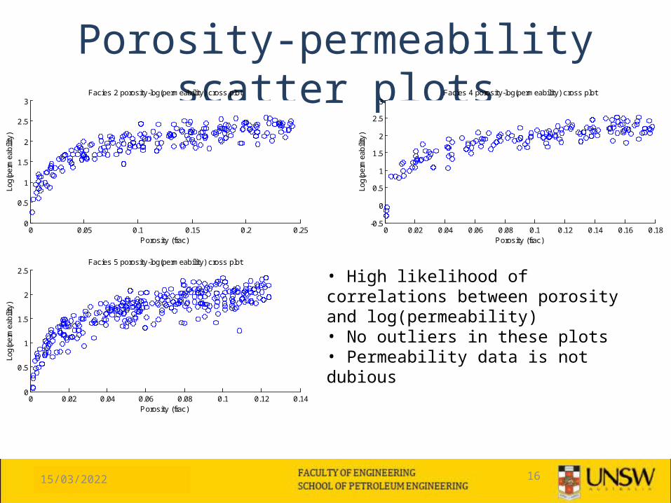
Porosity-permeability scatter plots
0 0.05 0.1 0.15 0.2 0.250
0.5
1
1.5
2
2.5
3Facies 2 porosity-log(permeability) cross plot
Porosity (frac)
Log(
perm
eabi
lity)
0 0.02 0.04 0.06 0.08 0.1 0.12 0.14 0.16 0.18-0.5
0
0.5
1
1.5
2
2.5
3Facies 4 porosity-log(permeability) cross plot
Porosity (frac)
Log(
perm
eabi
lity)
0 0.02 0.04 0.06 0.08 0.1 0.12 0.140
0.5
1
1.5
2
2.5Facies 5 porosity-log(permeability) cross plot
Porosity (frac)
Log(
perm
eabi
lity)
• High likelihood of correlations between porosity and log(permeability) • No outliers in these plots• Permeability data is not dubious
15/04/2023 17
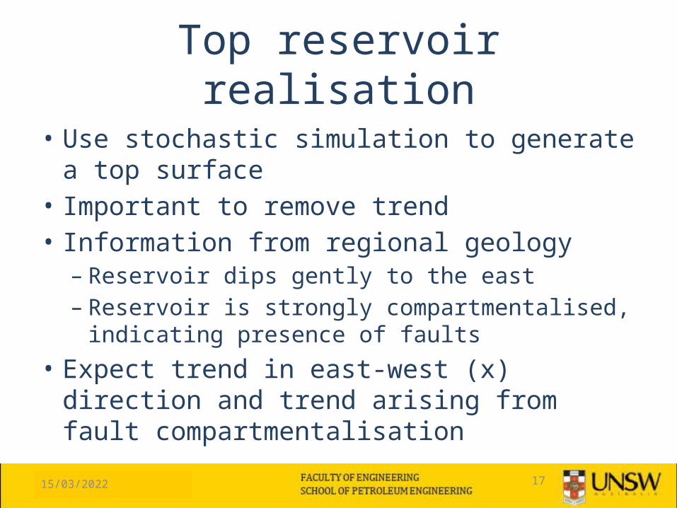
Top reservoir realisation
• Use stochastic simulation to generate a top surface
• Important to remove trend• Information from regional geology
– Reservoir dips gently to the east– Reservoir is strongly compartmentalised,
indicating presence of faults• Expect trend in east-west (x) direction and
trend arising from fault compartmentalisation

15/04/2023 18
Well top markerssorted in x direction
20 40 60 80 100 120 140 160 1802920
2940
2960
2980
3000
3020
3040
3060
x grid no. vs. top
x grid no.
Top
(m)
Faults
Grid 50Shift ~ 20m
Grid 150Shift ~ 10m
15/04/2023 19
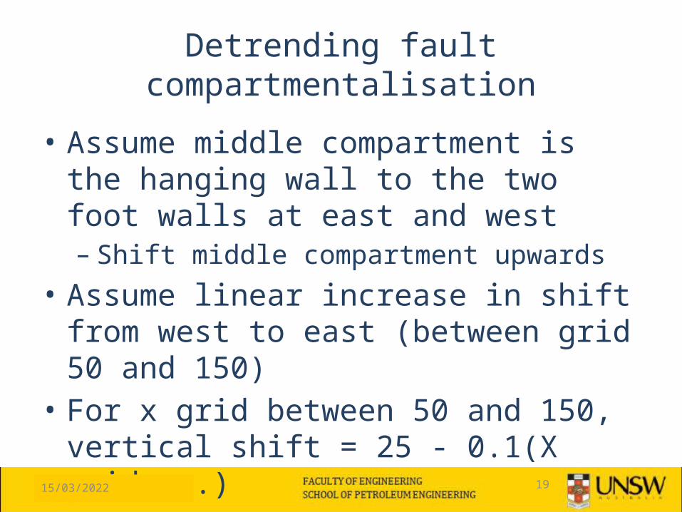
Detrending fault compartmentalisation
• Assume middle compartment is the hanging wall to the two foot walls at east and west– Shift middle compartment upwards
• Assume linear increase in shift from west to east (between grid 50 and 150)
• For x grid between 50 and 150, vertical shift = 25 - 0.1(X grid no.)
15/04/2023 20
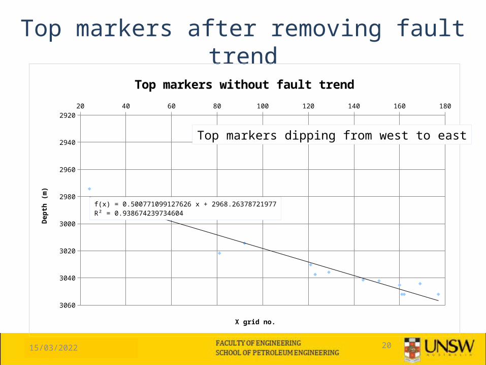
Top markers after removing fault trend
20 40 60 80 100 120 140 160 1802920
2940
2960
2980
3000
3020
3040
3060
f(x) = 0.500771099127626 x + 2968.26378721977R² = 0.938674239734604
Top markers without fault trend
X grid no.
Dept
h (m
)
Top markers dipping from west to east
15/04/2023 21
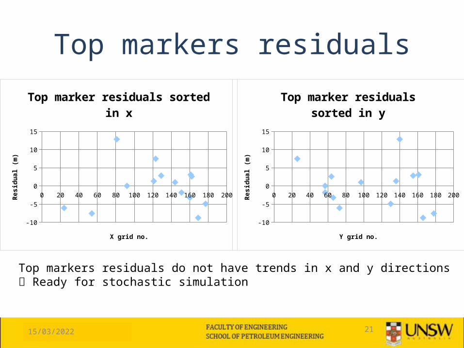
Top markers residuals
0 20 40 60 80 100 120 140 160 180 200
-10
-5
0
5
10
15
Top marker residuals sorted in x
X grid no.
Resid
ual (
m)
0 20 40 60 80 100 120 140 160 180 200
-10
-5
0
5
10
15
Top marker residuals sorted in y
Y grid no.Re
sidua
l (m
)
Top markers residuals do not have trends in x and y directions Ready for stochastic simulation
15/04/2023 22
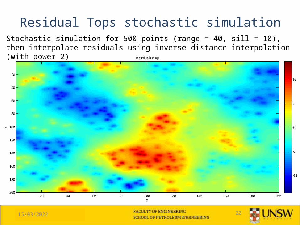
Residual Tops stochastic simulation
X
Y
Residuals map
20 40 60 80 100 120 140 160 180 200
20
40
60
80
100
120
140
160
180
200
-10
-5
0
5
10
Stochastic simulation for 500 points (range = 40, sill = 10), then interpolate residuals using inverse distance interpolation (with power 2)
15/04/2023 23
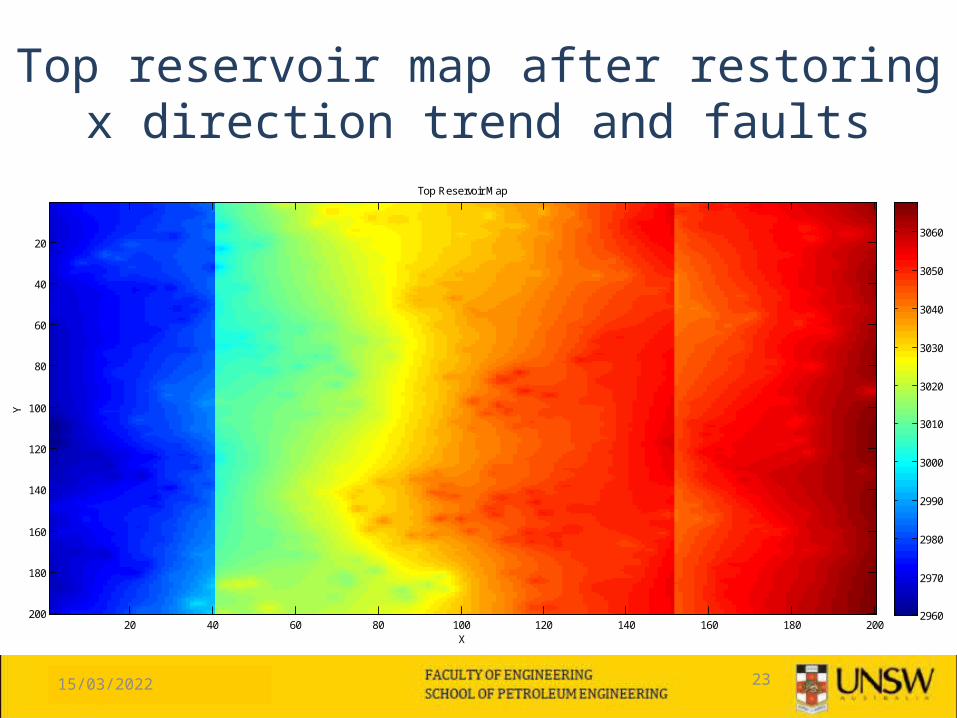
Top reservoir map after restoring x direction trend and faults
X
Y
Top Reservoir Map
20 40 60 80 100 120 140 160 180 200
20
40
60
80
100
120
140
160
180
200 2960
2970
2980
2990
3000
3010
3020
3030
3040
3050
3060

15/04/2023 24
Bulk rock volume calculation
• Since oil-water contact (owc) is within the reservoir, it is assumed to be the bottom of the reservoir
• Area of each cell is 10m by 10m• Reservoir thickness at each location = owc –
top • Bulk rock volume = 231MMm3

15/04/2023 25
Pore volume in hydrocarbon zone (HPV)
• HPV estimation requires net-to-gross and porosity values
• Approach: estimate net volume and average sandstone porosity at each well location– Assume facies 2, 4 and 5 are clean sandstone
net-to-gross of 1– Facies 1 and 3 are pure shale net-to-gross of 0
• Use stochastic simulation, generate net volume map and average porosity map
15/04/2023 26
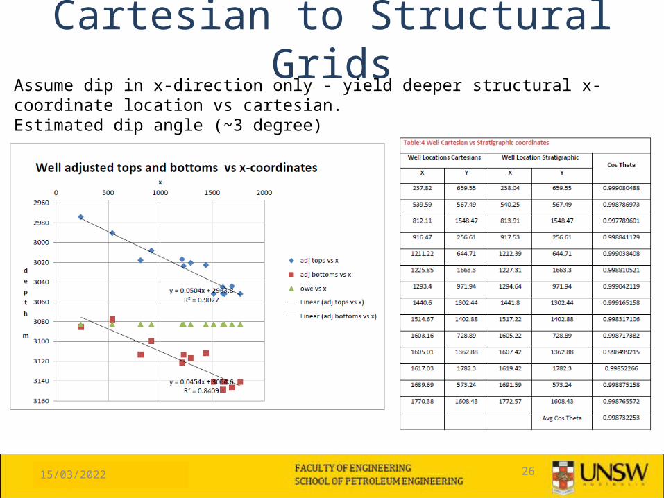
Cartesian to Structural GridsAssume dip in x-direction only - yield deeper structural x-coordinate location vs cartesian. Estimated dip angle (~3 degree)
15/04/2023 27
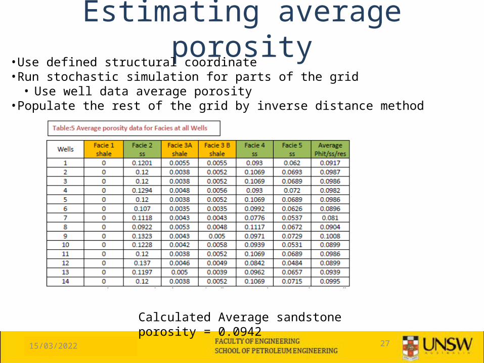
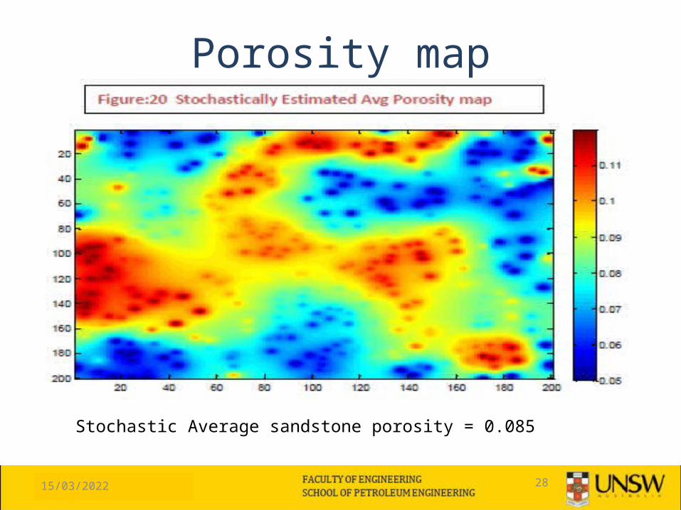
Estimating average porosity•Use defined structural coordinate•Run stochastic simulation for parts of the grid
• Use well data average porosity•Populate the rest of the grid by inverse distance method
Calculated Average sandstone porosity = 0.0942
15/04/2023 28
Porosity map
Stochastic Average sandstone porosity = 0.085
15/04/2023 29
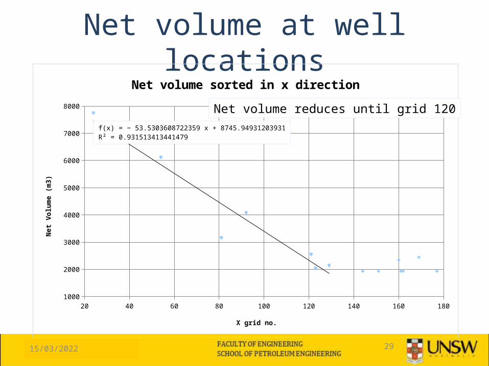
Net volume at well locations
20 40 60 80 100 120 140 160 1801000
2000
3000
4000
5000
6000
7000
8000
f(x) = − 53.5303608722359 x + 8745.94931203931R² = 0.93151341344148
Net volume sorted in x direction
X grid no.
Net
Vol
ume
(m3)
Net volume reduces until grid 120
15/04/2023 30
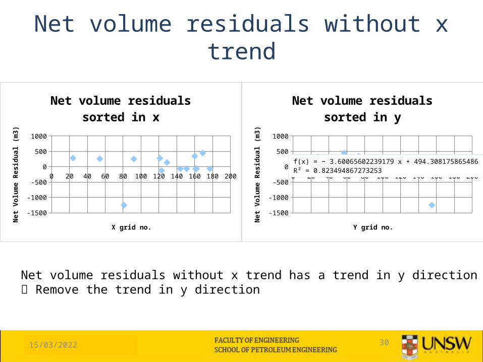
Net volume residuals without x trend
0 20 40 60 80 100 120 140 160 180 200
-1400
-1200
-1000
-800
-600
-400
-200
0
200
400
600
Net volume residuals sorted in x
X grid no.
Net
Vol
ume
Resid
ual (
m3)
0 20 40 60 80 100 120 140 160 180 200
-1400
-1200
-1000
-800
-600
-400
-200
0
200
400
600
f(x) = − 3.60065602239179 x + 494.308175865485R² = 0.823494867273253
Net volume residuals sorted in y
Y grid no.
Net
Vol
ume
Resid
ual (
m3)
Net volume residuals without x trend has a trend in y direction Remove the trend in y direction
15/04/2023 31
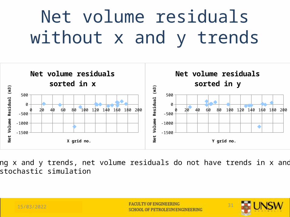
Net volume residuals without x and y trends
0 20 40 60 80 100 120 140 160 180 200
-1400-1200-1000
-800-600-400-200
0200400
Net volume residuals sorted in x
X grid no.
Net
Vol
ume
Resid
ual (
m3)
0 20 40 60 80 100 120 140 160 180 200
-1400-1200-1000
-800-600-400-200
0200400
Net volume residuals sorted in y
Y grid no.
Net
Vol
ume
Resid
ual (
m3)
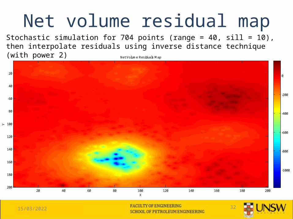
After removing x and y trends, net volume residuals do not have trends in x and y directions Ready for stochastic simulation
15/04/2023 32
Net volume residual mapStochastic simulation for 704 points (range = 40, sill = 10), then interpolate residuals using inverse distance technique (with power 2)
X
Y
Net Volume Residuals Map
20 40 60 80 100 120 140 160 180 200
20
40
60
80
100
120
140
160
180
200
-1000
-800
-600
-400
-200
0
15/04/2023 33
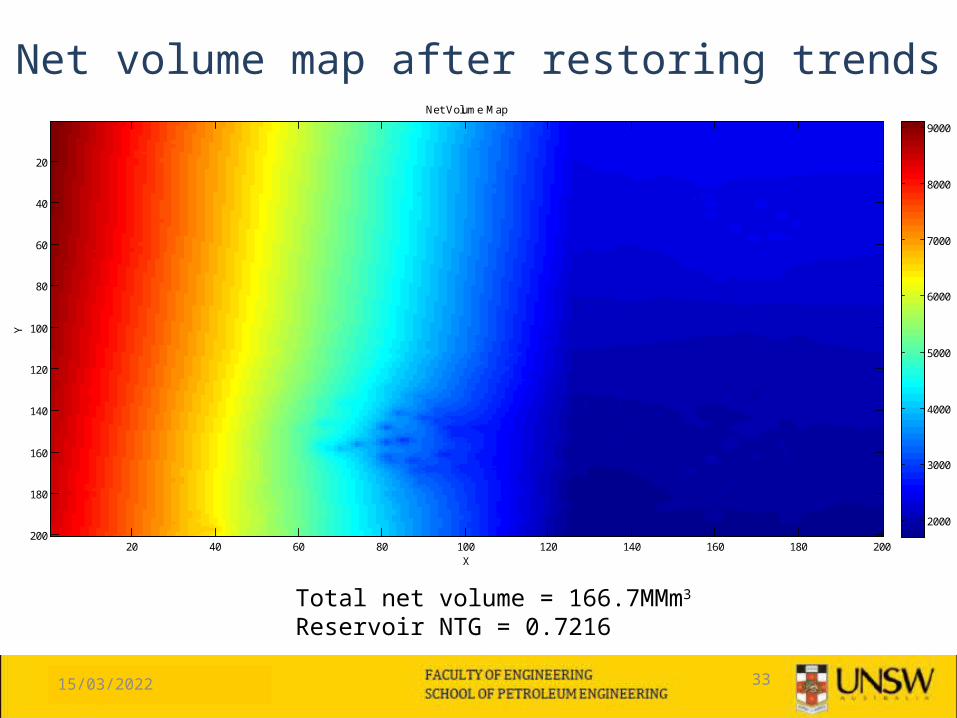
Net volume map after restoring trends
Total net volume = 166.7MMm3
Reservoir NTG = 0.7216
X
Y
Net Volume Map
20 40 60 80 100 120 140 160 180 200
20
40
60
80
100
120
140
160
180
2002000
3000
4000
5000
6000
7000
8000
9000
15/04/2023 34
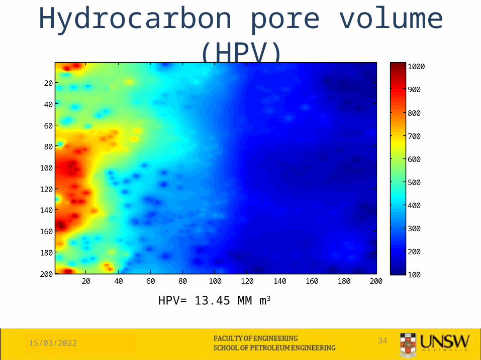
Hydrocarbon pore volume (HPV)
20 40 60 80 100 120 140 160 180 200
20
40
60
80
100
120
140
160
180
200 100
200
300
400
500
600
700
800
900
1000
HPV= 13.45 MM m3

15/04/2023 35
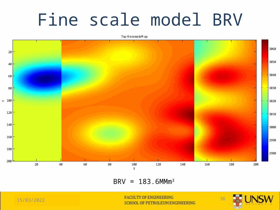
Fine scale model volume estimation
• Using similar methods to estimate BRV, HPV, reservoir NTG and average reservoir sandstone porosity
15/04/2023 36
Fine scale model BRV
X
Y
Top Reservoir Map
20 40 60 80 100 120 140 160 180 200
20
40
60
80
100
120
140
160
180
200
2980
2990
3000
3010
3020
3030
3040
3050
3060
BRV = 183.6MMm3
15/04/2023 37
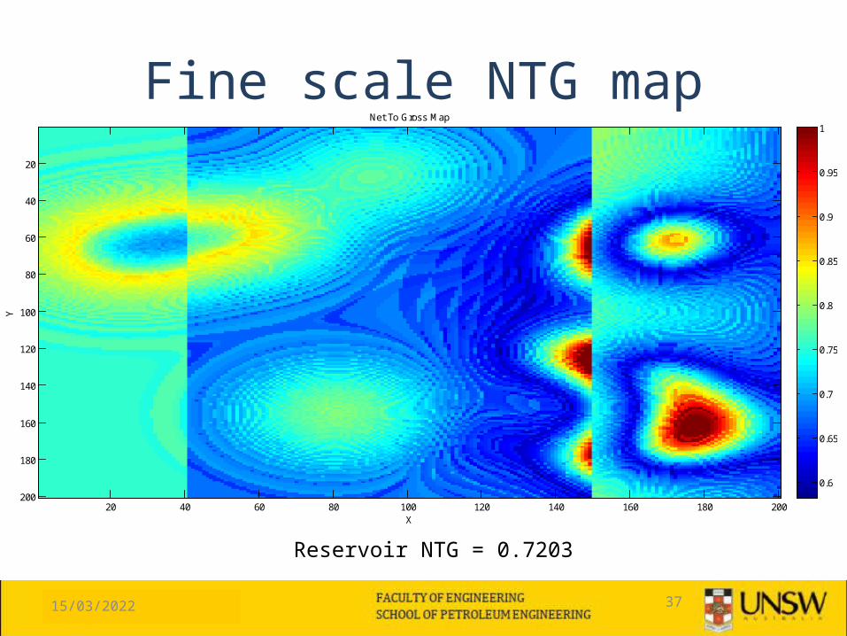
Fine scale NTG map
X
Y
Net To Gross Map
20 40 60 80 100 120 140 160 180 200
20
40
60
80
100
120
140
160
180
200
0.6
0.65
0.7
0.75
0.8
0.85
0.9
0.95
1
Reservoir NTG = 0.7203
15/04/2023 38
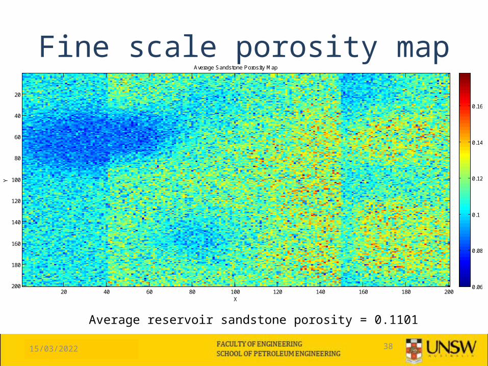
Fine scale porosity map
X
Y
Average Sandstone Porosity Map
20 40 60 80 100 120 140 160 180 200
20
40
60
80
100
120
140
160
180
200 0.06
0.08
0.1
0.12
0.14
0.16
Average reservoir sandstone porosity = 0.1101

15/04/2023 39
Fine scale HPV map
X
Y
Map of Pore Volume in Hydrocarbon Zone
20 40 60 80 100 120 140 160 180 200
20
40
60
80
100
120
140
160
180
200
200
300
400
500
600
700
Pore volume in hydrocarbon zone = 14.3MMm3
15/04/2023 40
Upscaling
• Upscale fine scale model from 2003 grids to 203 grids
• Upscale top reservoir map to calculate upscaled BRV
• Use facies values to upscale NTG• Use arithmetic average to upscale porosity
15/04/2023 41
X
Y
Top Reservoir Map
20 40 60 80 100 120 140 160 180 200
20
40
60
80
100
120
140
160
180
200
2980
2990
3000
3010
3020
3030
3040
3050
3060
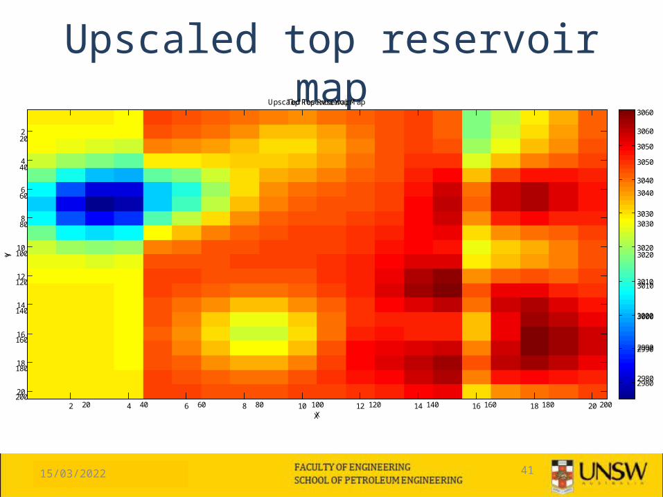
Upscaled top reservoir map
X
Y
Upscaled Top Reservoir Map
2 4 6 8 10 12 14 16 18 20
2
4
6
8
10
12
14
16
18
202980
2990
3000
3010
3020
3030
3040
3050
3060
15/04/2023 42
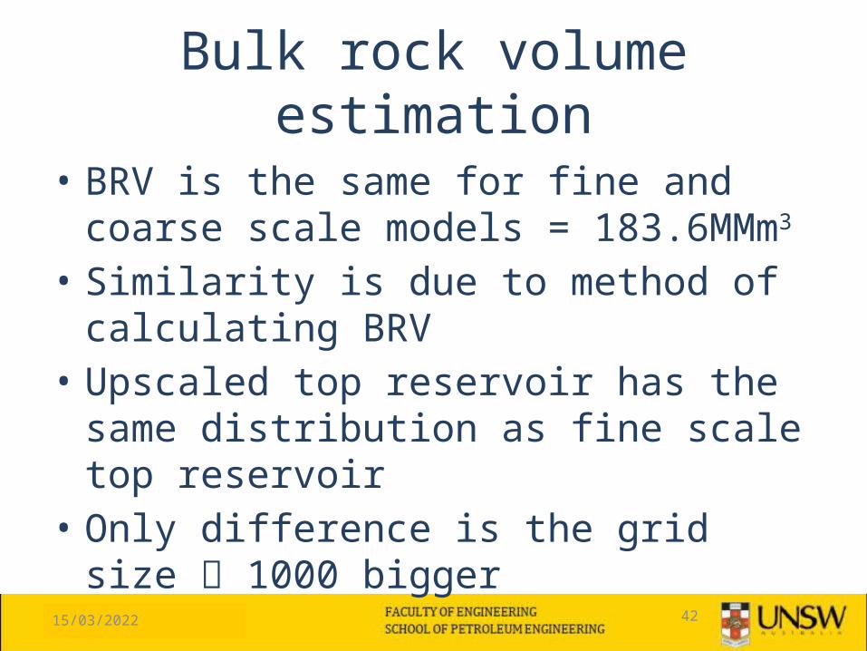
Bulk rock volume estimation
• BRV is the same for fine and coarse scale models = 183.6MMm3
• Similarity is due to method of calculating BRV• Upscaled top reservoir has the same
distribution as fine scale top reservoir• Only difference is the grid size 1000 bigger
15/04/2023 43
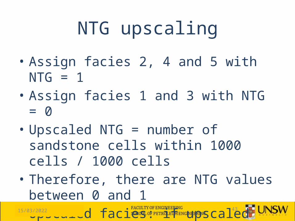
NTG upscaling
• Assign facies 2, 4 and 5 with NTG = 1• Assign facies 1 and 3 with NTG = 0• Upscaled NTG = number of sandstone cells
within 1000 cells / 1000 cells• Therefore, there are NTG values between 0
and 1• Upscaled facies: if upscaled NTG > 0.5
sandstone, otherwise it is shale
15/04/2023 44
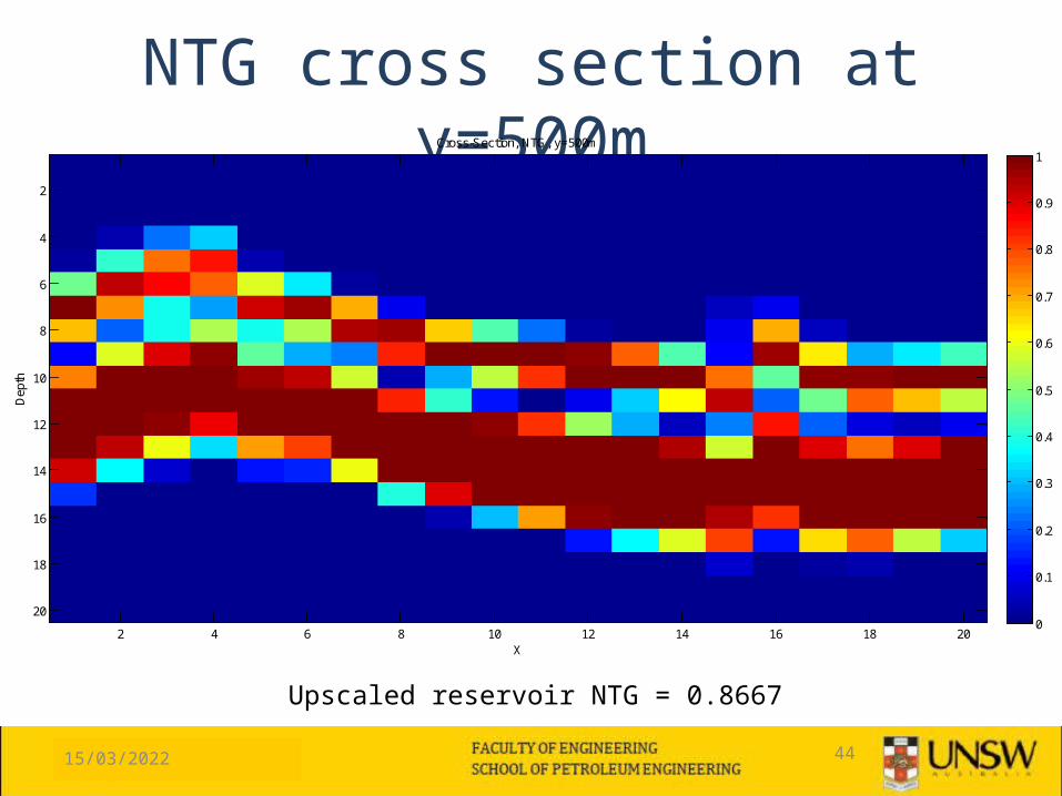
NTG cross section at y=500mCross-Section, NTG, y=500m
X
Dep
th
2 4 6 8 10 12 14 16 18 20
2
4
6
8
10
12
14
16
18
200
0.1
0.2
0.3
0.4
0.5
0.6
0.7
0.8
0.9
1
Upscaled reservoir NTG = 0.8667

15/04/2023 45
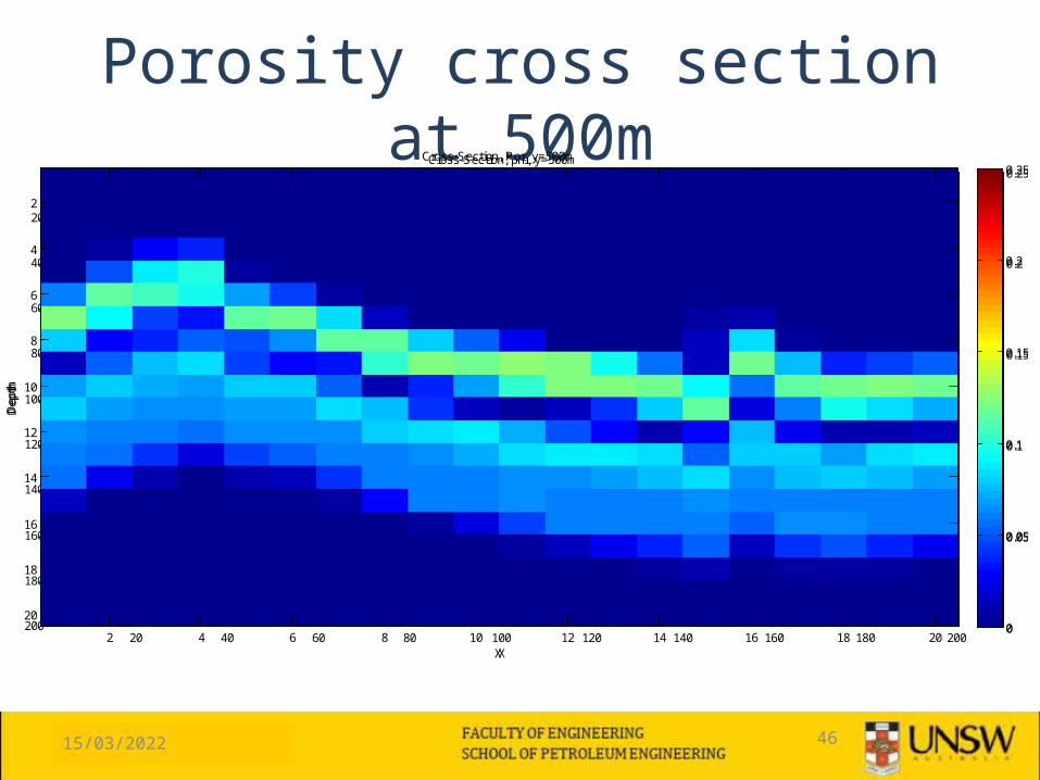
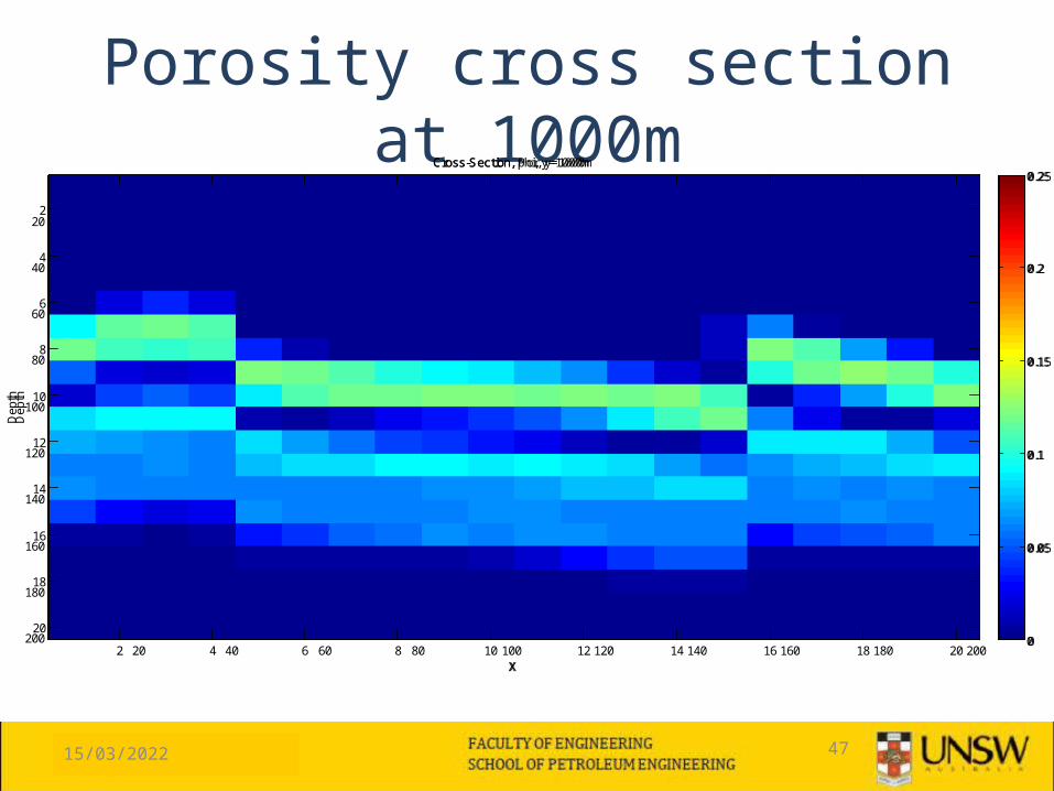
Porosity upscaling
• Porosity model is upscaled by taking the arithmetic mean of porosity within the 1000 cells grid
15/04/2023 46
Cross-Section, phi, y=500m
X
Dep
th
20 40 60 80 100 120 140 160 180 200
20
40
60
80
100
120
140
160
180
200 0
0.05
0.1
0.15
0.2
0.25
Porosity cross section at 500mCross-Section, Por, y=500m
X
Dep
th
2 4 6 8 10 12 14 16 18 20
2
4
6
8
10
12
14
16
18
200
0.05
0.1
0.15
0.2
0.25
15/04/2023 47
Porosity cross section at 1000mCross-Section, phi, y=1000m
X
Dep
th
20 40 60 80 100 120 140 160 180 200
20
40
60
80
100
120
140
160
180
200 0
0.05
0.1
0.15
0.2
0.25Cross-Section, Por, y=1000m
X
Dep
th
2 4 6 8 10 12 14 16 18 20
2
4
6
8
10
12
14
16
18
200
0.05
0.1
0.15
0.2
0.25

15/04/2023 48
Porosity cross section at 1500mCross-Section, phi, y=1500m
X
Dep
th
20 40 60 80 100 120 140 160 180 200
20
40
60
80
100
120
140
160
180
200 0
0.05
0.1
0.15
0.2
0.25Cross-Section, Por, y=1500m
X
Dep
th
2 4 6 8 10 12 14 16 18 20
2
4
6
8
10
12
14
16
18
200
0.05
0.1
0.15
0.2
0.25
15/04/2023 49
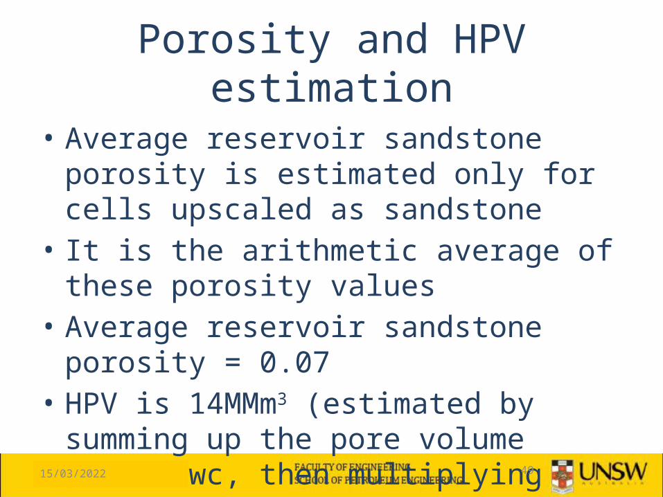
Porosity and HPV estimation
• Average reservoir sandstone porosity is estimated only for cells upscaled as sandstone
• It is the arithmetic average of these porosity values
• Average reservoir sandstone porosity = 0.07• HPV is 14MMm3 (estimated by summing up
the pore volume above owc, then multiplying with cell volume)

15/04/2023 50
Conclusions
• Stochastic simulation yields different realisations for different runs, especially when executed using only localised data like well data
• Volume estimations can have a big range and uncertainty

15/04/2023 51
Conclusions• The purpose of upscaling is to facilitate
dynamic simulation• It is important to maintain properties like
volumes during upscaling. In this project, pore volume in hydrocarbon zone is maintained, so the hydrocarbon reserves remain unchanged after upscaling
• As a result, reservoir net-to-gross and porosity are altered

15/04/2023 52
Recommendations
• Stochastic simulation can possibly yield a result with less uncertainty if seismic data is incorporated together with well data
• Better volume estimations can be conducted

15/04/2023 53
Q & A

15/04/2023 54
Possible top markers x trend without faults
0 20 40 60 80 100 120 140 160 180 2002920
2940
2960
2980
3000
3020
3040
3060
f(x) = − 0.0048796241209423 x² + 1.44614456150013 x + 2943.903806964R² = 0.963653116114509
x grid no. vs. top
x grid no.
Top
(m)
15/04/2023 55
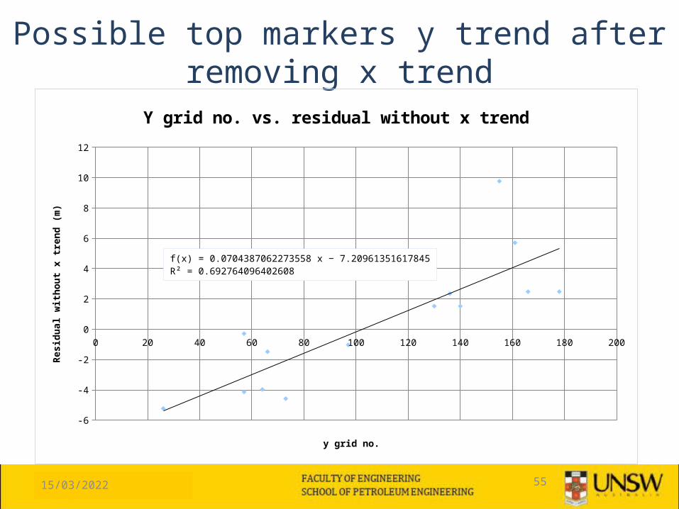
Possible top markers y trend after removing x trend
0 20 40 60 80 100 120 140 160 180 200
-6
-4
-2
0
2
4
6
8
10
12
f(x) = 0.0704387062273558 x − 7.20961351617845R² = 0.692764096402608
Y grid no. vs. residual without x trend
y grid no.
Resid
ual w
ithou
t x tr
end
(m)

15/04/2023 56
Residuals after removing x and y trends
0 20 40 60 80 100 120 140 160 180 200
-4
-2
0
2
4
6
8
Residuals sorted in x
X grid no.
Resid
ual (
m)
0 20 40 60 80 100 120 140 160 180 200
-4
-2
0
2
4
6
8
Residuals sorted in y
Y grid no.Re
sidua
l (m
)
15/04/2023 57
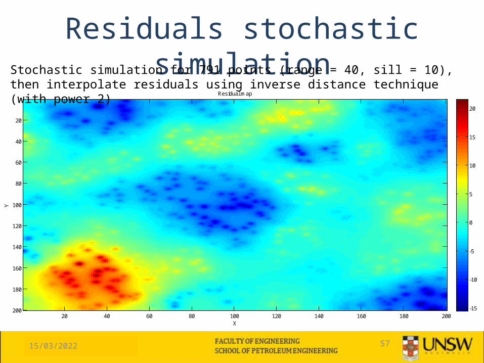
Residuals stochastic simulation
X
Y
Residual map
20 40 60 80 100 120 140 160 180 200
20
40
60
80
100
120
140
160
180
200 -15
-10
-5
0
5
10
15
20
Stochastic simulation for 791 points (range = 40, sill = 10), then interpolate residuals using inverse distance technique (with power 2)

15/04/2023 58
Top reservoir map after restoring x and y trends
X
Y
Top reservoir map
20 40 60 80 100 120 140 160 180 200
20
40
60
80
100
120
140
160
180
2002940
2960
2980
3000
3020
3040
Bulk rock volume = 0.24km3

15/04/2023 59
Average sandstone porosity at well locations
20 40 60 80 100 120 140 160 1800.08
0.09
0.1
0.11
0.12
0.13
0.14
f(x) = 0.000267325763803992 x + 0.0790138651402766R² = 0.644465926534814
Average sandstone porosity sorted in x
X grid no.
Aver
age
sand
ston
e po
rosit
y (fr
ac)
15/04/2023 60
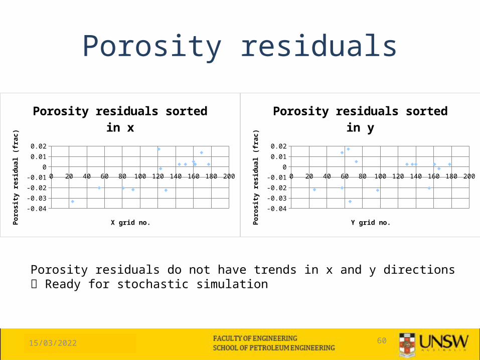
Porosity residuals
0 20 40 60 80 100 120 140 160 180 200
-0.04
-0.03
-0.02
-0.01
0
0.01
0.02
Porosity residuals sorted in y
Y grid no.
Poro
sity
resid
ual (
frac
)
0 20 40 60 80 100 120 140 160 180 200
-0.04
-0.03
-0.02
-0.01
0
0.01
0.02
Porosity residuals sorted in x
X grid no.
Poro
sity
resid
ual (
frac
)
Porosity residuals do not have trends in x and y directions Ready for stochastic simulation
15/04/2023 61
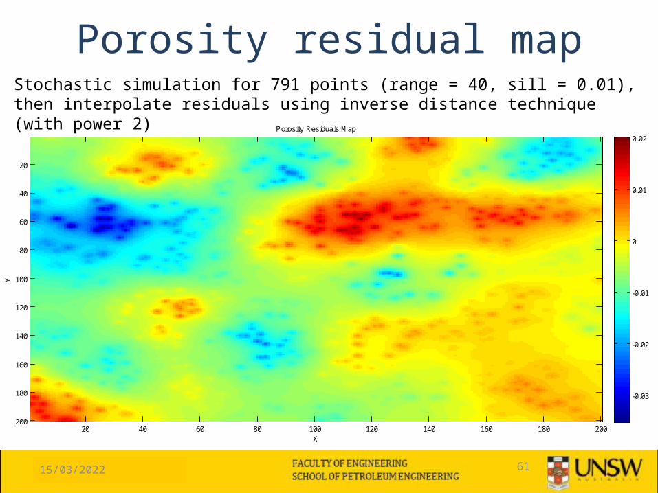
Porosity residual mapStochastic simulation for 791 points (range = 40, sill = 0.01), then interpolate residuals using inverse distance technique (with power 2)
X
Y
Porosity Residuals Map
20 40 60 80 100 120 140 160 180 200
20
40
60
80
100
120
140
160
180
200
-0.03
-0.02
-0.01
0
0.01
0.02
15/04/2023 62
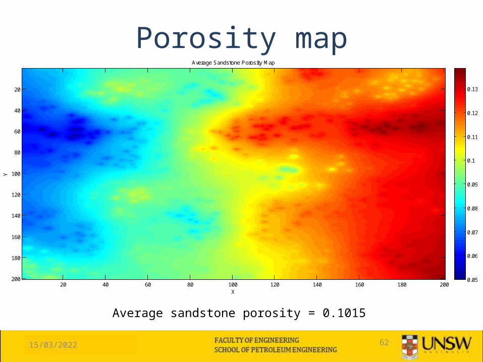
Porosity map
Average sandstone porosity = 0.1015
X
Y
Average Sandstone Porosity Map
20 40 60 80 100 120 140 160 180 200
20
40
60
80
100
120
140
160
180
200 0.05
0.06
0.07
0.08
0.09
0.1
0.11
0.12
0.13

15/04/2023 63
Map of pore volume in hydrocarbon zone
• Pore volume = net volume × porosity• OIIP =15.3MMm3
X
Y
Pore Volume Map
20 40 60 80 100 120 140 160 180 200
20
40
60
80
100
120
140
160
180
200200
300
400
500
600
700