Simulating Thermomechanical Phenomena of Nanoscale Systemsalexgreaney.com/media/publications/Greaney_2011... · 5.2.4 Nanoscale Phenomena In addition to the greater range of thermal

CHAPTER 5

Simulating ThermomechanicalPhenomena of NanoscaleSystems

P. ALEX GREANEY AND JEFFREY C. GROSSMAN

Department of Materials Science and Engineering, 13-5049 MIT,7 Massachusetts Avenue, Cambridge, MA 02139-4307, USA

5.1 Introduction

The manner in which we use and control heat is of great importance bothtechnologically, and within our daily lives. Roughly 90% of the energy that weuse today has been involved in the generation to and conversion from heat (e.g.,coal or gas power plants, combustion engines for transportation, and nuclearenergy, to name only a few). The efficiency of these processes is limited by thecontrol we have over the storage and transport of heat within materials. Mostpractical thermal-energy systems that are involved in transport, storage, and/orconversion operate far from their limits.Since thermal transport is a materials phenomenon, it is useful to compare

our understanding of it with other transport properties such as the conductionof electrons. Since the discovery of electricity, research on charge transport inmaterials has pushed the extremes of electrical conductivity, which now spansover 20 orders of magnitude. In 1947 the transistor was invented, which per-mitted external tuning of electrical conductivity in the solid state—and formingthe foundation for information processing and beginning the digital age. Thesocietal impact of research in electrical conduction has been and will continue

RSC Theoretical and Computational Chemistry Series No. 4

Computational Nanoscience

Edited by Elena Bichoutskaia

r Royal Society of Chemistry 2011

Published by the Royal Society of Chemistry, www.rsc.org

109

to be enormous. In contrast, heat transport in condensed matter has receivedmuch less attention. For example, the thermal conductivity of current solidmaterials spans only 5 orders of magnitude at room temperature and itsexternal tunability is limited. With the exception of the Carnot limit to heatengines, we really do not know what limits, if any, exist regarding the funda-mental processes of thermal energy transport and conversion, and storage.There are currently no thermally superconducting materials, nor are anyexisting materials perfect thermal insulators.An equivalent paradigm shift in thermal transport would be the use of fre-

quency-dependent thermal properties; that is, exploiting properties of materialsthat depend on the thermal energy being concentrated at specific frequencies.Such opportunities may exist in new thermal phenomena that occur in nanoscalematerials. The aim of this chapter is to provide an overview of the methods forsimulating thermal phenomena at the nanoscale. After giving a brief overview ofsome of the experimental progress that is driving this field we survey the currentcomputational methods highlighting their strengths, and the major challengesthat still face the simulation of heat. This is followed by two detailed case studiesin which selected methods have been used to study nanoscale thermomechanicalbehaviour, showing how these tools can be used, and what insight they can give.The examples given are in the study of dissipation in CNT resonators, and fre-quency-dependent heat transport across weak nanoscale interfaces. The chapterfinishes with a discussion of the major challenges still facing simulation of heat,and the outlook to new applications of thermal properties.

5.2 Examples of Recent Experimental Progress

There have been recently a number of exciting advances in our ability to controlheat flow that have primarily been achieved with the use of nanoscale systems.Accompanying the advances in engineering thermal properties have beenbreakthroughs in or ability to measure thermal transport and to characterizethermal behaviour at this small scale. Together, these experimental develop-ments show that we can extend the current boundaries of thermal conductance,and they call on scientists to develop more accurate and predictive methodsfor computing thermal conductance and for simulating thermomechanicalphenomena in nanoscale systems. A brief survey of the experimental advancesin nanoscale thermal properties that is motivating the need for new computa-tional approaches is given here.

5.2.1 Increasing Thermal Conductivity

As long ago as 19411 it was recognised that the mean free path of longitudinalacoustic phonons diverges as their frequency approaches zero.i In the absenceof internal scattering mechanisms this would mean that a material’s thermal

iAn infinitely long-wavelength mode is a quasistatic compression that must have an infinite meanfree path in order to satisfy Newton’s laws.

110 Chapter 5

conductivity would increase with the size of the material. In bulk materialsthere are a plethora of defects, interfaces and other scattering mechanisms thatlimit the mean free path, and make the thermal conductivity size invariant inpractice. Single-walled carbon nanotubes and graphene sheets are composed ofa single layer of atoms and are not bulk materials (one cannot distinguishbetween a surface and an internal atom in a CNT). With no interfacial scat-tering the only mechanisms for restricting the mean free path of long-wave-length modes are anharmonic phonon interactions and isotopic effects. Theresult of this is that single-walled CNTs can exhibit very large thermal con-ductivity along their length, and that the tubes must be very long (up to 10 mm)before k stops increasing with tube length.2–5 CNTs hold much hope forengineering new materials with very efficient thermal conduction for uses inthermal management; however, much of the heat transported along a CNT isconveyed by flexural and torsional modes. These important heat-carryingmodesonly move unimpeded when the CNT is free standing; the modes are quicklyscattered if the CNT is in contact with a substrate (or another CNT) reducing thethermal conduction by as much as two orders of magnitude.6,7 Nevertheless,applications have been proposed for using CNTs as heat guides. A very recentand innovative application has been to use CNTs as a heat guide to set up rapidlypropagating thermal reactionwaves in a reactingmedium.8 Bundles of CNTs arecoatedwith an exothermically reactivemixture, andwhen the reaction is initiatedrapid heat conduction along the tube speeds up the propagation speed of thereaction front. Most interestingly the passage of the reaction front has beenfound tobe accompanied by a large electrical thermopower pulse in the tubes thatis proportional to the speed of reaction propagation.The use of CNTs in other (nonreactive) thermal management applications

has also been demonstrated. Vertically aligned ‘‘forests’’ of CNTs have beenproposed for efficient thermal management of computer chips, where removalof heat can be the limiting factor in device performance, and where the powerdensities that must be removed can be extremely high.9 Vertically aligned foreststructures utilize the full thermal transport potential of the CNTs, limited onlyby contact resistance at the CNT ends. Other researchers have used embeddednetworks of CNTs to engineer highly anisotropic thermal conductivity incomposite materials and to tailor the cooling properties of oils with the addi-tion of a suspension of CNTs.10 In these cases the heat is carried across a sparsenetwork of CNTs. In order to travel long distances the heat must be passedbetween CNTs at the nexus points where they overlap within the network, andthis process has its own resistance, which is found to be large. Transport inthese networks—both electrical and thermal—exhibits a percolation transitionin which if the network is too sparse there are insufficient nodal connectionslinking the tubes and they will not create a contiguous pathway through thematerial. Remarkably, the percolation transition for conduction of electricityoccurs at a lower network density than it does for the conduction of heat.This is surprising as the networks are composed of CNTs with a distributionof different diameters and chiralities with roughly only one third of thembeing metallic; this implies that there is also a wide distribution of thermal

111Simulating Thermomechanical Phenomena of Nanoscale Systems

contact resistance, with many junctions being electrically conductive but highlyresistive to heat.

5.2.2 Reducing Thermal Conductivity

In crystalline solids a fundamental lower limit of thermal conductivity can beconceived by imagining that the mean free path of a phonon cannot be anyshorter than the intrinsic lattice spacing (similar conceptual limits can bederived for amorphous solids). These limits are somewhat artificial, however,being only a limit in which one model of heat flow no longer makes sense. Thus,while these limits can provide useful guidelines when designing thermal sys-tems, there are no rigid reasons why thermal resistance cannot surpass theselimits in some cases. This has in fact been observed experimentally forroughened Si nanowires11 that have been shown to transport heat below theperceived lower limit of conductance.Beyond the fundamental question on limits of thermal transport it is often

desirable to increase the thermal resistance of a given material without greatlyaltering other properties. An important technological example of this arethermoelectric materials, for which it is desirable to minimize lattice thermalconduction without altering the electrical properties of the material. In thiscase, one can take advantage of the fact that the mean free paths of chargecarriers (holes and electrons) are much smaller than the mean free path oflattice vibrations (phonon wave packets), and thus one can nanostructure thematerial on a length scale that will confound traveling-wave phonons, but thatis invisible to charge carriers. Experimentally, this was first approached bygrowing multilayered materials with controlled layer thicknesses. This is a top-down approach that allows one to finely control the structure at the angstromlevel in one direction. Another top-down approach is to create a nanoscalegrain structure in the material by deformation or powder processing. Thisapproach has been successful for further improving the thermopower ofestablished thermoelectric semiconductor materials.12 Examples of other moreexotic approaches to suppressing thermal conduction include roughenednanowires, nanoporous materials, and metamaterials that possess a phononbandgap. Recently, films containing nanoscale tubular pores running throughthe film thickness have been found to suppress thermal conductivity by severalorders of magnitude.13,14

5.2.3 Characterisation

In addition to advances in the ability to fabricate structures at the nanoscalethere has been significant progress in the ways that one can measure thermalproperties. Length-dependent thermal conductance has been measured onsingle CNT, and Si nanowires, lying across a set of heating stages.4,15–17 Usingthis approach Chang et al. demonstrated thermal rectification along carbon

112 Chapter 5

and boron nitride nanotubes that have been asymmetrically decorated withplatinum carbide.An alternative noncontact method of measuring heat transport properties in

nanoscale structures is by time-domain thermoreflectance. This is a pump-probe technique in which a short (pico or nanosecond) laser pulse locally heatsthe sample (raising the temperature by only a few degrees). The heating changesthe optical reflectance of the sample, and a probe laser beam is used to measurethis change in reflectance as the heat dissipates. Cahill and coworkers18,19 havefound that by making the region of material that is heated smaller than themean free path of some of the phonons these phonons leave the hot regionballistically, allowing one to measure the contribution of different phononfrequencies to thermal transport.

5.2.4 Nanoscale Phenomena

In addition to the greater range of thermal conductance that can be achievedwith nanoscale materials, the nanometer-sized systems provide new thermalphenomena that are unique to this length scale. Making one or two dimensionsof a system small (while leaving the others macro-or mesoscopically large)results in objects that are in effect two-, or one-dimensional. These objects stilllive in a three-dimensional space (mathematically they are said to have acodimension greater than one). Low-dimensionality systems possess new low-frequency phonon mode shapes in which the object deforms into the uncon-strained dimension. Films and surfaces gain surface Lamb waves, beams pos-sess flexural and torsional modes, and tubes and fullerenes have radialbreathing modes and cyclops modes.20

The symmetries of these low-dimensional modes can give rise to subtlethermal effects. Interatomic potentials are asymmetric, near equilibrium closeto harmonic, as we move further from equilibrium the potential softens as thebond is stretched and stiffens when compressed. The most important anhar-monic term in the representation of an atomic bond is the cubic term,d3Eij=dR3

ij : Yet the symmetry of a nanostructured material combined with thesymmetry of the vibrational mode can result in modes that are symmetrical,and where the fourth-order anharmonic term dominates. To see this, consider ananotube. Imagine sitting on the surface of a zigzag nanotube watching themotion of atoms as the tube undergoes a torsional oscillation. We see that foreach torsional cycle an atomic bond stretches twice; the mode is symmetricaland the cubic term in the bond potential d3Eij=dR3

ij results in a quartic termd4Etor=da4tor dominating the anharmonicity of the modes. Following the motionof the radial breathing mode (RBM), on the other hand, we see that it isasymmetric, and the cubic term d3ERMB=da4RBM dominates. Thus, through theincreased freedom of a codimension greater than one, it is possible to obtainvibrational modes with a mixture of differing symmetry of anharmonicity,although the structure is constructed with only asymmetric bonding potentials.Another simple example of this is a tensioned one-dimensional chain of atomsconnected by harmonic potentials. The ‘‘string-like’’ modes of the chain are


very strongly anharmonic because as the string oscillates the chain length isincreased, increasing the overall tension in the chain. This effect can result in anegative coefficient of thermal expansion along the chain length, and isobserved in carbon nanotubes that contract along their axis when they gethotter.21,22

Reducing the dimensionality of an object can cause other significant changesin properties. Diffusion in systems with two or fewer dimensions is spacefilling—that is given an infinite amount of time a random walker will visit everylattice site—this is not the case for three-dimensional spaces. A mathematicalconnection between diffusion and heat conduction results that heat flow in low-dimensional objects does not obeyFourier’s law. For the case of one-dimensionalsystems the thermal conductivity of the system is found to scale with the length ofthe system, k B La, with a being reported between 0.3,23 and 1/3.24 This hasimportant implications for modeling thermal transport in low dimensions: insimulation one often extrapolates the scaling of their results with system size inorder to estimate macroscale properties or to check convergence. This resultimplies that there is no length scale convergence in one-dimensional systems.

5.2.5 Quantum Phenomena

The examples given thus far are purely classical arising only due to restricteddimensionality; however, advances in characterisation and fabrication at thenanoscale have allowed researchers to measure several purely quantum effectsof atom motion. Roukes and coworkers, by cooling down a free-standing SiNmembrane supported by four phonon waveguides, were able to freeze out allbut the lowest-frequency vibrational modes in the waveguides and were able tomeasure ballistic conduction through just the four lowest-frequency modes(one longitudinal, two flexural, and one torsional) in each waveguide.25 Theyfound the quantum of thermal conductance, go, to match the Landauerequation go ¼ p2k2BT=ð3hÞ; approaching the quantum limit of measurement.A different quantum measurement effect that is close to the grasp of current

experimental methods is the direct observation of zero-point motion and theHeisenberg uncertainty in a mesoscopically large mechanical system. Gigahertznanoscale resonators can be frozen to their ground state at milikelvin tem-peratures, but one must also be able to sensitively detect the displacementsassociated with this motion which are on the subangstrom scale. Beyondestablishing that quantum-mechanical effects are observable in mechanicalsystems containing many billions of atoms, interesting applications for quan-tum computing are found if the system is coupled to a quantum-mechanicaltwo-level system.26

5.2.6 Far-from-Equilibrium Behaviour

Traditionally, the way that we have controlled and transport heat in solids hasbeen close to equilibrium—a usage that is reflected in the established theories of

114 Chapter 5

heat flow such as the Boltzmann transport theory (BTT) in which heat carrierstransport thermal energy between regions that are in local thermal equilibrium.In recent years, however, there have been examples of nanoscale devices (orphenomena) that take advantage of thermal behaviour far away from equili-brium, that is, where thermal occupation of vibrational modes does not cor-respond to the Bose–Einstein distribution (the local temperature is not welldefined) but is instead athermally distributed amongst the system’s vibrationalmodes. Operating away from equilibrium allows one to take advantage of themechanical properties of a system at a particular set of frequencies and thusenables the exploitation of a wider range of thermal behaviour than can beachieved at equilibrium.An athermal phonon population (APP) can arise in suspended carbon

nanotube (CNT) resonators through either frequency-specific Joule heating ofoptical phonons (at K and G),27–30 or by direct driving31,32 (or cooling33) oflow-frequency flexural modes. In the former case this causes the electricalconduction to saturate at high voltage, and in the latter the resulting APP candramatically reduce the resonator’s quality factor.34,35 APPs can also arisewhen heat is conducted across CNT interfaces.10,36 Taking advantage of theAPP leads to strategies for engineering interfacial thermal conductivity,37,38

and may be important in the recently discovered thermal power waves inCNTs.8 Biological systems can also display nonequilibrium thermal-energydistributions. Enzymatic reactions can result in a large heating of localisedmodes in the protein. This heat must be dissipated efficiently without dena-turing the enzyme, and is transferred through a restricted set of localisedvibrational modes without heating the enzyme as a wholeii.39,40 A similar‘‘energy funneling’’ phenomenon is observed in virus capsids41 in which laserheating of high-frequency modes is funneled into a handful of low-frequencymechanical modes—an effect that can may be exploited for selectivelydestroying harmful viruses.42 In the second of the case studies given later in thischapter we discuss APPs that arise from frequency-selective transmission ofheat in two weakly interacting objects, and we show how this can be exploitedfor applications in chemical sensing.

5.3 Survey of Simulation Methods

There are two approaches to computing thermal properties of nanoscale sys-tems. If the theory behind the property of interest is well understood one maycompute the property directly, perhaps using simulation or first-principlescalculations to obtain the values of input parameters. An example of thisapproach is the use of density-functional theory (DFT) to compute a material’sphonon density of states and then using that information to compute thespecific heat as a function of temperature. This approach works well for cal-culating intrinsic properties of a system that are not dependent on size orgeometry. An alternative approach that is valuable for system-specific

iiA similar concept is important for barrierless termolecular reactions.


properties is to use atomistic simulation to model the behaviour directly. Thisapproach can be thought of as performing an experiment within the computer(in silico) instead of in the laboratory. An advantage of direct simulation is thatas one has the full atomistic trajectory of the system in time it is often possibleto dissect the data to determine features that are contributing strongly to thephenomenon under study, and to gain insight into how one can alter the systemto change it. Both approaches—direct calculation, and computer experiment—are important and complementary as will become evident in the rest of thischapter.One of the most important thermal properties for engineering applications is

the thermal conductivity of a material, j, which is defined by the phenomen-ological Fourier’s law that relates the steady-stateiii thermal flux, JQ, to thelocal temperature gradient:

JQ ¼ �j � rT : ð5:1Þ

Here, we review several well-established methods for predicting the latticecontribution to k at the nanoscale. Calculation of k provides good examples ofboth direct computation approaches and in silico experiment, and in thiscontext we discuss the general advantages and challenges of these twoapproaches (beyond just computing k). At the end of this section we go beyondthe mean thermal conductance to examine far-from-equilibrium thermalbehaviour, and the methods can be used as the basis of studying other ther-momechanical phenomena in nanoscale systems, as will be shown in the casestudies that follow this section.

5.3.1 Direct Computation of j

In crystalline solids, heat is carried by moving scattering lattice vibrations, andone can therefore write the thermal flux using the Boltzmann transport equa-tion (BTE):iv

JQ ¼X

branches

ZN0

o�hbnðoÞlðoÞruðoÞ@Nðo;TÞ

@TrT : ð5:2Þ

Here, the sum is performed over all phonon branches and polarisations, andn (o), l (o), and ru (o) are, respectively, the group velocity, mean free path,and volumetric density of states for phonons with frequency o. b is a

iiiWe restrict discussion to the steady-state properties. Inclusion of time dependence to Fourier’s lawignores the fact that heat travels with a finite velocity and thus for describing transient thermalsolutions one must use the relativistic heat conduction equation, or the Cattaneo equation, whichis beyond the scope of this chapter.

ivNote that the BTE is a very general equation for describing the motion of particles in a fluid that isaway from equilibrium. Only in 2010 has the general form of the equation been rigorously provenfor systems close to equilibrium. For simplicity, we jump straight to the form appropriate for themotion of a phonon gas, and further simplify by assuming isotropy so that k becomes a scalarquantity rather than a tensor.

116 Chapter 5

dimensionless geometric factor and N(o, T) is the number of phonons occu-pying a mode with frequency o at temperature T. Strictly, one must solve for N(o, T) self-consistently; however, close to equilibrium this can be approximatedby the Bose–Einstein distribution.The BTE is very general and may be extended to include the ballistic con-

tributions to transport that can occur in very small systems. Computing kbecomes a matter of computing b, n, l, and ru, and the accuracy of one’sprediction relies on how accurately each of these terms are computed. Theterms n and ru can be computed from first-principles methods. The physics ofscattering in the system is encapsulated in the mean free path term and includes:3- and 4-phonon anharmonic scattering processes; electron–phonon interac-tions; and scattering from surfaces, interfaces, and impurities. The detail withwhich one includes these factors will determine the ultimate accuracy of theprediction.One important advantage of directly calculating k from the BTE is that

the quantum mechanical nature of heat is treated correctly—both in termsof the selection rules for phonon creation and annihilation, and the occupationof the vibrational spectrum. The difficulty is in quantifying all the detailedgeometry-specific phonon transition rates.In a system with a high degree of disorder, propagating phonon states are

not well defined and the phonon gas model of transport is no longer appro-priate. Allen and Feldman43 and others have developed a model descriptionrelevant to such a system. They classify the quanta of vibrational energy(vibrons) in an amorphous system into: propagons, that reside in low-frequencyplane-wave-like modes; diffusons, that reside in nonlocalised but non-propagating (stationary) modes; and locons, that occupy high-frequencylocalised modes that are above the mobility edge. The majority of heat con-ducted through these systems is mediated by phonon transitions between dif-fusion modes.

5.3.2 Computing j by Direct Simulation

Amaterial’s intrinsic resistance to conducting heat is due tophonon scattering thatstems from anharmonicity in the interatomic interactions. As enumerating andcomputing all the scattering processes is difficult, a potentially more appealingapproach is simply to accurately compute the anharmonicity of the atomic inter-actions and then use this withinmolecular dynamics (MD) simulations tomeasurethe thermal conductivity in silico. The simulationwill numerically account for all ofthe phonon-scattering processes without having to identify them a priori.The most intuitively straightforward method for computing k in this manner

is to impose a thermal gradient in a system and simulate it using MD. Onecan straightforwardly set up a molecular dynamics simulation in which two(distant) slabs of atoms within a solid are thermostatted to different tempera-tures. By measuring the work done by the thermostats at each side of thisthermocouple one finds the heat current that is transported down the thermalgradient in the intervening material between the slabs. However, while this


approach most resembles a real experiment, it is fraught with severalchallenges, some that are common to all MD simulations, and some (such asthe size of the simulation cell and the use of thermostats) that can be overcomewith more carefully designed simulations.In the computational setup described above, the temperature in the inter-

vening material does not vary smoothly between the two thermostatted regionsbut experiences a discontinuous step at the boundary with the thermostattedregions—making the temperature gradient hard to control computationally.More significant, (especially in terms of computational affordability) is that thecomputational cell must be large enough to accommodate the mean free path ofthe heat-carrying phonons; and these can be several hundreds of nanometers.While this is large from the point of view of computational tractability, it isoften still very small compared to the temperature difference, resulting in alarge DT, which can throw into question the validity of the linear responseapproximation.An alternative approach is to switch the roles of cause and effect, so that

rather than impose a temperature gradient one imposes a fixed thermal flux byadding (non-net-translational) kinetic energy at a constant rate to the atoms inone region, and removing heat at the same rate in the cold slab. This procedurewas first developed by Muller-Plathe44 and is often referred to as reversenonequilibrium molecular dynamics (RNEMD). The approach is applicable tomany transport phenomena and is also used for computing the viscosity offluids.45 The approach still suffers from requiring a very large computationalcell but the system converges to the steady state more rapidly than the directnonequilibrium MD approach described above.It is possible to move away from the nonequilibrium approaches altogether,

and instead to simulate a system at equilibrium in the microcanonical ensemble(NVE) and make use of the fluctuation-dissipation theorem that relates thelinear response properties of a system out of equilibrium to the dissipation ofthermal fluctuations within the system at equilibrium. The Green–Kubomethod46 relates the thermal conductance k, to the autocorrelation function ofthe fluctuations in the heat flux JQ, at equilibrium:

k ¼ 1

T2kBV

ZN0

dtCðtÞ; ð5:3Þ

with kB the Boltzmann constant, V the volume of the cell and the correlationfunction C(t) defined by:

CðtÞ ¼Z

dtJQðtÞJQðtþ tÞ ¼ JQðtÞ; JQðtþ tÞ� �

; ð5:4Þ

JQðtÞ ¼dR

dt; ð5:5Þ

118 Chapter 5

R ¼Xi

rihi: ð5:6Þ

Here, the term R can be considered the centre of energy, as the sum of thepositions of all atoms weighted by the sum of their potential and kineticenergies.v One advantage of the Green–Kubo method (in addition to its com-putational simplicity) is that as the heat-flux correlation function decays muchmore rapidly than the heat-carrying phonon’s mean lifetime, the system sizethat must be simulated can be many times smaller than is required for none-quilibrium MD methods.47

For all of their intuitive appeal, using MD simulation to in silico measure ksuffers from several important and fundamental challenges, the most importantof which is that the simulations are classical—that is, the trajectories of theatoms are integrated according to Newtonian mechanics without any quantum-mechanical phenomena included. This is usually justified by stating that formost elements at room temperature the atoms are sufficiently heavy that theirde Broglie wavelength is negligible and the atoms can be treated classically.A notable exception is hydrogen, whose small mass does make quantum-mechanical effects significant and makes simulation of water particularlytroublesome.77 While this reasoning is true it overlooks two other quantumeffects, first, that the permitted energy of vibrational modes is quantised withoccupation En ¼ o�h nþ 1

2

� �; and that the quanta of energy (that we refer to as

phonons, not the modes that they occupy) are bosons and so fill the availablestates according to the Bose–Einstein distribution.This has two consequences: First, not all modes have a uniform amount of

energy—low-frequency modes will hold more energy than higher-frequencymodes according to relation EiðTÞh i ¼ oi�h=expðoi�hbÞ � 1, where, b ¼ 1=kBT ,is the reciprocal temperature. At temperatures below the Debye temperature,TD, the high-frequency modes with be unoccupied and will possess only theirzero-point energy. This stands in direct contrast to a classical system in whichall the modes may have a continuum of energy, and where on average all themodes will have the same energy regardless of the temperature. For this reasonmolecular dynamics simulations are usually performed at temperatures aboveTD, where at least the participation of all vibrational modes is a reasonableassumption (although the filling of the modes is still incorrect). Alternatively,simulations may be performed at low temperatures if the phenomena of interestonly involves low-frequency modes, and if it can be shown that the activity ofhigh-frequency modes does not influence the behaviour of these low-frequencymodes.The second consequence of the quantum harmonic oscillator is that when

heat is transferred from one mode to other modes (i.e. when phonons are

vThe potential energy of an atom can be poorly defined for many-body potentials; however, it isusual to approximate the local bonding energy to be shared between participating atoms in apairwise fashion.


created and annihilated) the participating phonons must follow strict selectioncriteria such that the sum of the frequencies of the participating modes beforeand after the transition event are equal. No such restrictions are present inclassical systems. The importance of this for MD simulations is that one cannotassume that the processes observed are directly transferable to real quantum-mechanical systems. Goddard and coworkers have shown that in the case ofdiamond at temperatures above TD, the quantum correction to the classicalGreen–Kubo calculated k is small.47

Besides the fundamental quantum-mechanical deficiencies of MD simula-tions there are also some practical considerations. Thermodynamic propertiesare an ensemble average over all the possible states of the system. While inprinciple MD simulations are ergodic and will correctly sample phase space thetime it takes to do so is very long, much longer than the duration that can befeasibly achieved in a single simulation. In a single MD simulation the systemstrajectory only samples a narrow region of phase space, if we are to properlyaverage over phase space we must run many simulations starting with verydifferent initial conditions in order to attain a representative sampling on theensemble.

5.3.3 Gaining Insight from Simulations

Despite the many limitations and deep-rooted challenges for simulating ther-mal phenomena with MD methods, it is still a widely used tool that can bepowerful for gaining physical insight if it is used judiciously. The main reasonfor this is that one knows the positions and velocities of every atom in thesystem during a MD simulation (knowledge that is out of reach from a realexperiment). Armed with this raw data it is often possible to tease out subtlemechanisms of heat transport, scattering, and dissipation. This can be parti-cularly useful when designing structures that suppress or enhance the mobilityof phonons within a particular band of frequencies. Extending the analogy ofthe computer experiment these methods are like the characterisation tools ofthe real experimenter: they do not interfere with the physics used to simulate thesystem, but are used to interpret the results of simulation. The last part of thisreview of computational methods focuses on these numerical ‘‘characterisa-tion’’ methods for distilling insight from raw MD simulation data.Considerable insight can be gained simply by watching an animation of

atomic motion in an MD simulation. One gains a mental picture of what theatoms are doing and one can quickly spot anomalous behaviour. As a methodthis is not very rigorous, it is a challenge to be sure that the animation isrepresentative of the statistical ensemble, and it is difficult to disseminatemovies in the traditional publishing format. However, the human brain is verygood at spotting visual patterns (sometimes too good, finding patterns that arenot there): watching a movie of simulated atom motion can quickly help one toidentify bugs, or spot whether seemingly interesting results are merely artifactsof the system setup. It can also help identify interesting and physically

120 Chapter 5

meaningful behaviour on which more sophisticated and rigorous numericalcharacterisation methods can be trained.A more rigorous method of ‘‘watching’’ the atoms was employed with great

success by Phillpot, et al.48 These researchers launched phonon wave packets athigh-angle grain boundaries in Si and taking snapshots of the average kineticenergy of the atoms within slices of the computational cell, they followed theenvelope of vibration as it collided with the interface, and were able to identifythe mixture of scattered and transmitted wave packets. The method was used todetermined which vibrational frequencies are transmitted most efficientlyacross the grain boundaries.Much information can be learned from the vibrational spectrum of a

nanoscale object, which as was mentioned above, can differ greatly from bulksystems. One consolation of the classical limitations of MD is that we cancompute the vibrational spectrum (more or less) for free from any equilibriumMD simulation that we perform by Fourier transforming the autocorrelationfunction of the total kinetic energy. This can be done for any temperature, andwhile the spectrum must be weighted by the Bose–Einstein distribution toobtain the correct intensities the MD will capture the shift in mode frequenciesdue to filling of anharmonic modes.The zero-temperature phonon spectrum for a nanoscale system can also be

computed directly by diagonalising the Hessian matrix or the dynamical matrix(depending on whether the system is molecular or extended). Both of thesemethods have the advantage that in addition to the frequencies of the modes,one also obtains their eigenvectors. For very large systems with many millionsof atoms, finding all the eigenvectors becomes computationally expensive;however, one can search sequentially for the lowest-frequency modes byrecasting the matrix diagonalisation as an energy-minimisation problem, amethod developed by Sankey et al.49 for computing atomistically the vibra-tional modes of virus capsids.Knowing the eigenvectors for the vibrational modes permits one to search

through them, classifying the modes based on their symmetry or their spatialcharacter, and to identify which modes are dominating the thermal phenom-enon under study. For example, if one has a complex system of weakly inter-acting molecular units, such as a double-walled CNT, it permits one to identifymodes that are confined to each individual CNT and those modes that areshared between the tubes. Obviously the shared modes will be most importantfor transmitting heat between the inner and outer walls of the CNT.There are other ways of classifying modes based on their spatial extent. Allen

and Feldman et al.50 have classified the modes of amorphous Si, into propa-gating, diffusive, and localised modes. The lowest-frequency modes extendacross the full extent of the system and can be thought of as propagating wave-like deformation modes. The wavelengths are much longer than the scale of thestructural heterogeneity and the mode feels the average mechanical propertiesof the material—the limit being the infinite-wavelength mode corresponding toa homogeneous eigenstrain. At intermediate frequencies the modes becomeweakly localised, in that the wavelength of the modes becomes comparable to


their mean free path. Above this so called Ioffe–Regal limit51 the modes arediffusive, and the majority of heat is transported by energy exchange throughthese modes. The highest-frequency modes are short and localised aroundstructural anomalies. These transport little heat and are said to be above themobility edge.Various approaches for measuring the degree to which a mode is localised

have been developed by different researchers. Galli et al.14,52 have computed the‘‘participation ratio’’, p of the eigenmodes in a number of nanoscale systemswith one or two reduced dimensions. The participation ratio of mode i is ameasure of the fraction of atoms in the system that are participating in thedisplacement of this mode and is defined as:

pi ¼1

N

XNj¼1ðeij � eijÞ2

!�1; ð5:7Þ

where N is the total number of atoms, and eij is the displacement vector of the

jth atom due to mode i withPNj¼1

eij � eij ¼ 1: Fully delocalised modes have p

ranging between 1 and 0.5 with localised modes having smaller p with the limitthat a mode localised to a single atom has p¼ 1/N. Yu and Leitner40,53 havesorted the vibrational modes of a large protein molecule by their exponentiallocalisation length, x by best fitting exp (|r – ro|/x) to the decay of the mode’samplitude away from the mode’s centre (ro). Using this approach, an inversecorrelated was found between localisation length and mode frequency.Armed with the knowledge of some or all of the vibrational modes of a

system one can project these modes onto the atomic displacements and velo-cities at any time during an MD simulation to obtain the instantaneousamplitude, a(t), and velocities, _aðtÞ; of the modes.

aiðtÞ ¼XNj¼1

eij � ðrjðtÞ � roj Þ; ð5:8Þ

_aiðtÞ ¼XNj¼1

eij � tjðtÞ: ð5:9Þ

From computing the velocity of individual modes in this way during anequilibrium MD simulation one can calculate the mode’s lifetime, ti, by inte-grating the normalised autocorrelation function of the mode velocity.6,54

Integrating gives the time it takes for the velocity autocorrelation function todecay, which is the average time after which the oscillation has lost coherencewith itself. Galli and coworkers have shown the power of this approach bymultiplying the computed lifetimes by the phonon group velocity, ng (the gra-dient of the phonon dispersion) to calculate the phonon mean free paths,l¼ ngt. The mean free path appears in the BTE (eqn (5.2)), and thus computingthis from simulation permits one to attribute each mode’s contribution to thetotal heat transport.

122 Chapter 5

Mode projection also yields insightful information from nonequilibriumMDsimulations where knowledge of the modes not only allows one to analyse theresults of a simulation but also excite a simulation away from equilibrium in acarefully chosen way. Adding an instantaneous velocity and/or displacement tothe system along a mode’s eigenvector excites a single vibrational mode. Afterexcitation, by simulating in the microcanonical ensemble one can follow thesystem as it relaxes back to equilibrium. This scheme has been widely used foruncovering the detailed mechanisms of energy transfer in a diverse array ofsystems, including: phonon scattering at grain boundaries,48,55 energy relaxa-tion within protein molecules41,56 and damping in CNT resonators.34,35 Moredetailed examples of the use of the phonon projection are given in the two casestudies later in this chapter. Here, we give a pedagogical discussion offrequency-dependent energy transfer. The aim is to show the types of infor-mation that can be gleaned from MD simulations using mode projection, andsome of the areas in which care must be taken.As a test system, let us consider the case of two identical carbon (10, 0)

carbon nanotubes. The tubes are lying adjacent and parallel to each other, andthey are weakly bound together by the van der Waals interactions betweenthem. The tubes are (10, 0) tubes with a 4.2-nm periodic repeat distance, andthey are in a vacuum. Full details of the simulation setup can be found in ref 36.After optimising the structure of an isolated single tube, its eigenmodes arecomputed using the frozen phonon method. Note that this only gives stationarysolutions, not traveling modes—it is equivalent to diagonalising the dynamicalmatrix at G for the whole computational cell. The second identical tube is nowintroduced and the system is again optimised—the two tubes are attracted toeach other and flatten very slightly where they ‘‘touch’’ to maximize thisattraction. The normal modes of the isolated CNT are not the normal modes ofthis new composite system; nevertheless, it is instructive to interpret the transferof energy in terms of the modes of the isolated CNT. We now excite just onemode in one CNT by displacing it. In this example, we choose the radialbreathing mode RBM of the left-hand CNT that we call tube A.vi The system ofthe excited and relaxed tube is simulated in the microcanonical ensemble. Modeprojection is used to compute the amplitude and velocity of each mode mea-sured relative to the ground state of the relaxed double-tube structure at everytimestep (roj in eqn (5.8) is the atomic positions in the optimised double-tubesystem). Before the projection is performed care must be taken to unwrap anyatoms that have crossed the periodic boundaries, and if the tube has randomlyrotated it must be mapped back into the orientation in which the Hessianmatrix was computed. The set of mode energies at a time t are represented as asmoothed spectrum by summing a set of Lorentzian functions centred at the

viBesides the mode that has been externally excited, the tubes are at absolute zero. This is anunusual and hypothetical situation that is seemingly problematic for classical dynamics. However,as all modes have zero energy using classical mechanics it is justified any time t¼ 0. Moreover, aswe are only following the first stages of the relaxation of this energy before all become classicallyoccupied, the use of MD remains justified for the short timescale simulated here. The simulationswere repeated at finite temperatures and the same behaviour was observed.


mode frequencies and weighted by the mode energies. This approach toobtaining the vibrational spectrum is considerably more computationallyexpensive than the velocity correlation method, and less straightforward toimplement; however, it gives us the excited spectrum at every time step, ratherthan averaged over some simulation time. Plotting the instantaneous spectrumagainst time gives the surface plots shown in Figure 5.1.Examining the plots in Figure 5.1 reveals a surprising amount of information.

First, we can follow the first cascade of energy as the excitation of theRBM in the‘‘hot’’ CNT relaxes towards equilibrium. Four distinct energy-transfer eventsare distinguishable: (a) First, energy is transferred resonantly from the RBM inthe hot tube to the RBM in cold tube. The transfer is frequency-selective and thefrequency of the heat is preserved after being exchanged between tubes; (b) Next,the energy in the cold tube’s RBM is scattered anharmonically into a mode withexactly half the frequency of the RBM. It can be shown by examining theeigenmodes that this frequency halving transition arises because the RBM isasymmetrically anharmonic whereas the half-frequency mode is not;36 (c) Thehalf-frequency mode in the cold tube transfers the excitation resonantly backto the equivalent mode in the hot tube, where (d) some of the energy isanharmonically scattered back into the initially excited RBM.In addition to following the cascade of energy transitions, the projection data

reveals much information about the nature of the participating modes.While theprojection scheme computes the exact instantaneous kinetic energy of each

Figure 5.1 Plots showing the relaxation of the excited RBM in one of a pair of parallelcarbon nanotubes. Four distinct energy transfer events are distinguishable:(a) hot tube resonantly exchanges energy fromRBMintoRBMin cold tube,(b) energy is scattered anharmonically within cold tube from RBM into amodes with half the frequency, (c) resonant exchange of energy from coldtube to hot between half frequency modes, and (d) anharmonic scatteringwithin hot tube from half frequency mode to RBM.

124 Chapter 5

mode, the potential energy is only estimated using the harmonic approximation.This inaccuracy can be used to our advantage. Comparing the over-(and/orunder) estimation of the potential energy with the kinetic energy of a modeprovides important information regarding the degree of anharmonicity in themode, whether the anharmonic terms stiffen or soften the mode, and whetheranharmonicity is asymmetric (as is the case for the radial breathing mode of aCNT). This information can be compared with and corroborated by computingthe frequency shift of the mode relative to the frozen-phonon limit (computedfrom the power spectrum of the mode’s velocity autocorrelation function).Comparing the amplitudes of a mode’s potential and kinetic energy can also beused to identify nonresonant oscillations. The row of small peaks below 1 THz inthe spectra of both the hot and cold tubes are an example of this. It is found thatthis oscillation has very little kinetic energy and is mostly comprised of a quasi-static elastic deformation of the low-frequency flattening modes of the tube. Theexcitation is artificial, and is not caused by these modes oscillating but by amuchslower oscillation between the two tubes as awhole. The tubes ‘‘chatter’’ togetherunder the influence of the van der Waals interaction. As the tubes come closetogether they flatten slightly (like a bouncing tennis ball) and it is the deformationof this flattening that gives rise to the serrated row of peaks.Thus far, we have discussed the use of mode projection as a characterisation

tool for interpreting the results of MD simulation; however, as mode projectiongives information about the instantaneous state of the system there is no reasonwhy this information cannot be fed back into the simulation and used to directit. For example, knowing the eigenmodes of a system and using projection todetermine their occupancy allows one to envision using external driving forcesto regulate the energy in specially selected modes. This could be used for:continually driving a system away from equilibrium (as is done experimentallyin driven nanomechanical resonators); enforcing a Bose–Einstein occupation ofthe classical modes; or even in schemes for efficiently searching phase space forrare events. While such procedures are not yet widely used they are beingactively developed. Praprotnik et al. have shown that molecular dynamics canbe performed efficiently in phonon space just as easily as in Cartesian space,57

while Parinello et al.58 have developed a Lengevin thermostatting algorithmthat uses history-dependent (that is, correlated) noise to drive particular fre-quency modes without the need for mode projection. The continued develop-ment of these types of algorithms means that MD—for all of its classicalshortcomings—will continue to be an important and powerful tool for studyingnanoscale thermal behaviour both at equilibrium, and far from it.

5.4 Example: Heat Flow in a Nanoscale Material;

Intrinsic Dissipation in CNT Resonators

Carbon nanotubes possess a number of properties that make them attractivefor use as resonating members in many nanoscale devices. The use of CNTresonators has already been demonstrated as a radio tuner,59 an entire radio


receiver,60 and a radio transmitter.61 In addition, CNT resonators have beenused to measure minuscule masses,31 even down to the mass of a single Auatom,32 and to approach the quantum limits of vibration.62 In addition to thesedemonstrated applications the potential uses for CNT resonators are muchbroader, being applicable to any nanoscale device that requires controlledvibration, such as gyroscopes, mechanical processing of signals, and simplemechanical time keeping. The reason why CNTs are so suitable are multifold:CNTs’ extraordinarily high stiffness combined with their low density enablesthem to attain very high natural frequencies, and frequency sensitivity. ThatCNTs are quasi-one-dimensional or string-like provides well-defined strategiesfor tuning their frequency—for example one may alter their length or put themunder tension. Finally, CNTs can be both driven, and sensed, electronically bya number of different methods, making it possible to integrate CNTs into morecomplex nanoelectromechanical systems (NEMS) in which the resonator isonly one part of the device.To date, the biggest impediment to the use of CNTs as resonators is their

very poor quality factor, Q, which when measured at ambient temperatures(and under conditions of constant driving) falls in the range of 8–300. (Q isdefined to be 2p times the inverse fraction of oscillator energy lost per cycle, andmay be thought of as roughly the number of oscillations it takes for the energyto be reduced by 99.8%.) This result has been resistant to improvement, havingbeen observed both under vacuum and at ambient pressure; in both cantilev-ered and doubly clamped geometries with many different clamping methods;and through many different measurement techniques.31,63–66 Only recently bycooling to milikelvin temperatures have Qs in excess of 105 been attained.62 Theuniversally poor ambient temperature results suggest that an intrinsic dampingmechanism may be dominant. Macro- or mesoscopic theories of intrinsicdamping from sources such as switching of defect states, thermoelastic damping,and phonon drag relate dissipative behaviour to the thermal energy in the system,that is, the background temperature Tbg. These theories have been successfullyused to describe dissipation in some nanoscale systems, particularly those wherephonons are diffusive and phonon lifetimes are shorter than the period of theresonator. Roukes et al.67,68 and others69 have suggested that the intrinsic ther-moelastic damping mechanism is capable of producing very low Q factors inCNTs due to their very small surface-to-volume ratio—although otherresearchers disagree on the importance of this mechanism.70 Previous compu-tational work by Jiang et al., of an open-ended, cantilevered CNT foundQ¼ 1500 at 293 K, with the unexpected temperature dependence: QBT –0.36,although the authors did not explicitly identify an intrinsic damping mechanism.The question of whether a poor quality factor is intrinsic is one into which

in silico experiments can lend considerable insight. In the computer, one cansimulate a carefully chosen idealised test system in which all extrinsic sources ofdissipation have been removed. Simulating such a system it is possible to see:First, if intrinsic damping alone can account for the poor Q factors; and sec-ond, to identify the mechanisms of intrinsic damping with the goal of findingways to mitigate them. We recently performed such a study that leads to the

126 Chapter 5

discovery of a new and surprising dissipation mechanism—one that can yieldMpemba-like behaviour in the cooling of an excited mode. The work isdescribed here in order to serve as one example of how computational methodscan be used to gain insight into nanoscale thermal phenomena.The messy system of a doubly clamped suspended CNT resonator was

represented in the idealised test system as a short section of a periodicallyrepeated (along its axis) single-walled CNT, isolated in a vacuum and free fromdefects and mass impurities. This setup removes dissipation sources from defectmigration, clamping friction, and gas damping. The effect of periodic boundaryconditions is to add a clamping of sorts by restricting the number and wave-length of the CNT’s flexural modes. The frequencies of flexural modes in theunclamped tube are higher than the modes of the same wavelength in thedoubly clamped counterpart as there is no centre-of-mass motion. Instead ofsimulating the resonator under conditions of constant driving—as is the casefor the experimentally measured Q—the resonator was simulated in themicrocanonical ensemble as an initially excited flexural mode was allowed tothe ring-down.A typical simulation proceeded as follows: (1) The structure of a (10,0) CNT

(simulated using the AIREBO potential for carbon–carbon interactions71) wasrelaxed, and the periodic repeat distance optimised.vii (2) the stiffness matrixfor the system was computed and then diagonalised to yield the tube’seigenmodes, and their frequencies. (3) The tube was heated to a desiredbackground temperature, Tbg, and allowed to equilibrate. (4) An instanta-neous velocity was added to the system along one particular eigendirection(usually that of the second flexural mode) such that the total average tem-perature of the system is raised by the amount Tex. (5) Ring-down wassimulated (NVE) during which the vibrational energy distribution in all of themodes of the CNT is tracked using the mode-projection algorithm describedabove. The excitations of the flexural mode were large; however, despite theenergetic excitations it was found that the mode remained reasonablyharmonic, containing at most a 5% anharmonic contribution to the potentialenergy.This study relies extensively on in silico experiments to investigate dissipation

mechanisms. It is therefore imperative to ensure that the computationalmethods used are meaningful. It should be noted that the simulations wereperformed using classical molecular dynamics at temperatures well below theDebye temperature for the CNT. This is justified a posteriori by the findingthat it is low-frequency modes that are participating in the dissipationmechanism. Simulating at low temperatures allows observation of the dis-sipation with little obfuscating thermal noise, and therefore is preferable if itcan be physically justified. Leaving aside the issue of mode occupancy,a more fundamental problem is the use of classical mechanics to simulate the

viiThe length of the tube was typically 8.4 nm, which it should be noted has an aspect ratio con-siderably lower than a typical NEMS resonator, and additionally possesses no residual axialtension. The short tube length was chosen to reduce the computational cost of the mode-pro-jection scheme.


dissipation of an energy that is quantised. Yet, as a more suitable methodthat includes quantised dynamics is lacking, classical dynamics is used withthe understanding that the physical interpretation of the results is limited.Similarly, interatomic forces were computed using empirical potentials thatwere formulated to capture the energetics of carbon and hydrogen bondingacross a range of bonding coordinations. There is no reason to expect thisto correctly represent the anharmonic character of the carbon–carbon bondin a CNT. Thus, it is necessary to verify the robustness of the reportedsimulation results to changes in interatomic potential. The results of thesimulations are found to be sensitive to changes in the interatomic potential;however, the overall qualitative behaviour is not. This may be in part becausethe dissipative behaviour is due to the shapes of the low-frequency modes,which are largely dictated by the tubular geometry rather than the detailsof the potential. As the qualitative trends do not depend on how the simu-lations are performed one is justified to draw general and meaningfulconclusions.The ring-down curves for the second flexural mode of a 8.4-nm long (10,0)

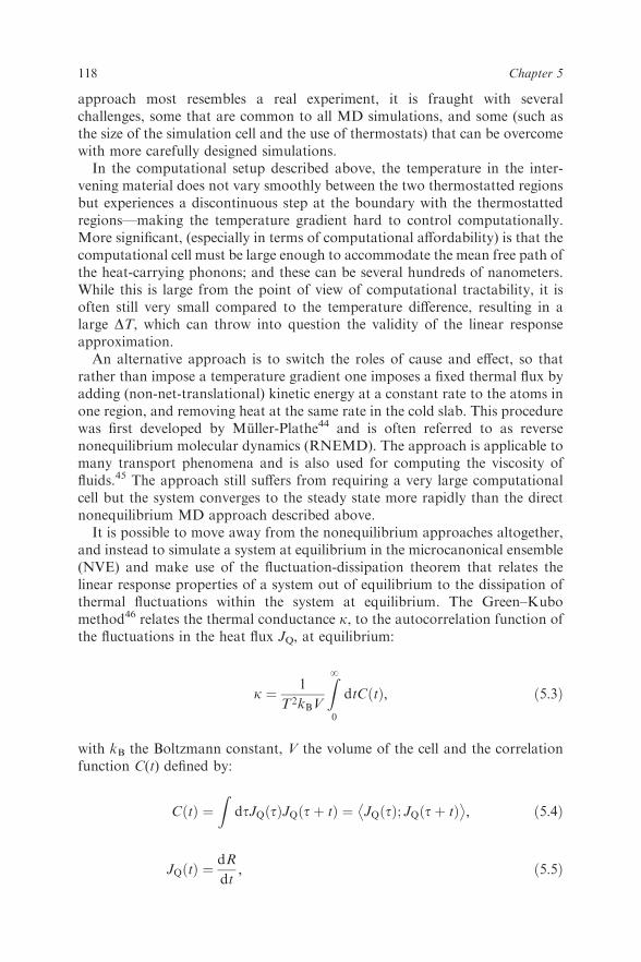
CNT, with a background temperature of Tbg¼ 5 K, and with increasing levelsof initial excitation is shown in Figure 5.2(a). It can be seen that the attenuationof the oscillation follows a sigmoidal path, with larger initial excitations beingcompletely damped in a shorter time than softer excitations. Figure 5.2(b)shows the ring-down profile for a 150 K excitation in tubes with increasingthermal background. As the background temperature rises the region of fastestattenuation is moved to earlier times.To interpret the attenuation profiles in Figures 5.2(a) and (b) it is instructive

to consider the attenuation of a simple damped harmonic oscillator withtemperature-dependent dissipation. The equation of motion for such anoscillator is given by

€u ¼ �o2u� BðTbgÞ _u; ð5:10Þ

where u, o, B, are respectively the oscillator’s displacement, (undamped) fre-quency, and mass-weighted drag coefficient, with the overdot indicating thederivative with respect to time. If the period of oscillation is short in com-parison to the attenuation time (o c B/2), then we may ignore the oscillatorybehaviour, noting instead that the rate at which energy is lost to drag is pro-portional to twice the kinetic energy, and thus the total energy in the oscillatordecays according to

_EðtÞ ¼ �BðTbgÞEðtÞ: ð5:11Þ

As a first approximation, the drag term is assumed to take the form of a first-order Taylor expansion: B(Tbg)¼BoþB0DTbg, with B0 positive. The increase inbackground temperature is simply the energy lost from the oscillator divided byC, the specific heat of the background, so that DTbg¼ (Eo – E(t))/C. Solvingeqn (5.11) gives the attenuation profile,

128 Chapter 5

EðtÞ ¼ EoBf

Bf � Bið1� eBf tÞ ; ð5:12Þ

(plotted in Figures 5.2(c) and (d)) where Bi¼B0 is the initial damping coeffi-cient, and Bf¼BoþB0Eo/C is the damping coefficient when the system is fullyrelaxed. This simple model displays many of the features of the moleculardynamics simulations in Figures 5.2(a) and (b), including an inflection in theattenuation profile (if the damping coefficient more than doubles as the systemrelaxes), as well as the trends that arise from independently increasing Tex orTbg. Using a simplified ‘‘toy’’ model such as this is often very instructive forinterpreting simulation results. In this case the model that might have initiallyseemed as surprising sigmoidal attenuation of the resonator’s ringing is entirelyconsistent with the computational setup. However, the model is also overlysimple and there are features in the simulation results that the model cannotcapture; still, by using the model as a starting point one can also learn where tolook for new and interesting behaviour.

(a) (b)

(c) (d)

Figure 5.2 Plots (a) & (b) show the MD simulated ring-down profiles for the secondflexural modes in 8.4 nm long (10,0) CNTs. In all cases the data is theaverage of 10 separate simulations with differing initial conditions;the data is plottedwith a broad line thickness chosen such that it encloses thedeviation of the averaged data. Plot (a) shows tubes with initial Tbg¼ 5 KandTex¼ 50, 100, 150, 200, and 300K. Plot (b) show the attenuation profilein tubes with initial Tex¼ 150 K, and Tbg¼ 5, 10, 50, 100, 150, 200, 400,and 400 K. Plots (c) & (d) show trends in simulation profile of a closed,damped harmonic oscillator (eqn (5.12)) when independently increasingTex, and Tbg, respectively.


5.4.1 Mpemba-Like Behaviour

A consequence of simulating in the microcanonical ensemble is that the CNT isa closed system; energy dissipated from the excited flexural mode accumulatesin the rest of the vibrational modes of the tube, raising Tbg. Increasing Tex

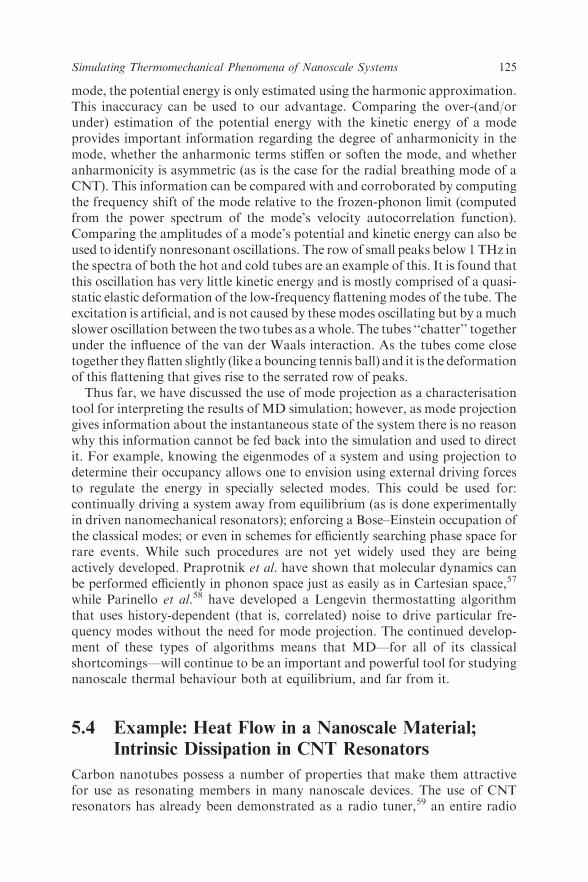
independently from Tbg changes the average temperature of the system andthus one would expect a different attenuation profile. More remarkable is thecooling of the excited mode in systems in which the same total energy,Tt¼TbgþTex, but differing initial partitioning of this energy between theflexural mode and the background (shown in Figure 5.3(a). Starting a simu-lation further from equilibrium (that is with larger initial Tex/Tbg) causes thesystem to reach equilibrium in a shorter time! We refer to this astounding, andcounterintuitive behaviour, as ‘‘Mpemba-like’’ in analogy with the Mpembaeffect72 in which it is observed that when hot water and cold water are put into afreezer the hot water freezes first.viii

While the dissipation mechanisms active during the cooling of water are verydifferent from the damping within a CNT we will see that in both cases thesystem is able to reach equilibrium faster because both systems contain ahidden variable, and in both cases the cooling results in changes in the hiddenvariable that do not follow a unique pathway.Figure 5.3(b) shows the ring-down time for increasing initial Tex in

systems for which TexþTbg¼ 300 K. Two measures of the ring-down timeare plotted: the time taken for excitation to be damped to a fixed lowerthreshold; and the interval over which the excitation is diminished by a setfraction—both measures decrease the further one starts from equilibrium. Aswith the Mpemba effect, relaxing faster to equilibrium the further one startsfrom it can only occur if the cooling pathway is not unique, but insteaddepends on the system’s initial conditions—as illustrated by the inset plot inFigure 5.3(a).From the ring-down profile of the simulated CNT resonator one can

compute the Q factor at any time t as QðtÞ ¼ �oEðtÞ=EðtÞ; where o is the

viiiThe Mpemba effect was and still is somewhat controversial. There are a number of differingexplanations for the phenomenon that range from the practical to the fundamental. An exampleof the former is the hot water in the ice cube tray melts a layer of surface ice on the freezer shelfthus making better thermal contact. Just one example of a fundamental explanation of theMpemba effect is that the cooling of the water is mediated by convection currents that haveinertia and momentum. Once established in a hot liquid—with a large driving force they aremaintained as the liquid cools. Cooling then depends on the average temperature T (which has nomemory) and the convective flow C (which is dependent on the liquid’s thermal history). Theconvective flow C provides the history-dependent hidden variable. The Mpemba effect is alsocontroversial because of the manner in which it became popularised—through the observationsof a Tanzanian school by George Mpemba (although the effect had been commented on muchearlier by other natural philosophers, including Aristotle and Francis Bacon73)—and how itseems to directly challenge intuitive scientific understanding. In fact the Mpemba effect makes nochallenge to established science or the scientific method, it only holds a mirror to the way that wedo science in prac tice and the barriers that we have for updating our personal intuitive scientificunderstanding when we are presented with more evidence. A good discussion of the Mpembaeffect, and its history is given by Jeng.73

130 Chapter 5

frequency of the excited mode.ix Figure 5.3(c) shows the change in the Q factoraccompanying the attenuation of a CNT. The Q drops from close to 1900 bymore than 95% to 37 and then is seen to recover towards 1000 after 20 ps.The origin of this huge suppression of the Q and its subsequent recovery can beunderstood by using the projection algorithm to track how the energy popu-lates the background modes once it has been dissipated from the flexural mode.The evolution of the background population is shown in Figure 5.3(d). It canclearly be seen that the energy goes first into low-frequency modes—close to thefrequency of the flexural mode—before dispersing across the full vibrationalspectrum of the CNT. This nonuniform filling of the background modes is dueto a small set of key ‘‘gateway modes’’ that act as strongly nonlinear channelsfor dissipation. These gateway modes and the role that they play is examined inmore detail later in this section. However, without knowing how the gatewaymodes work it can be seen that the nonequilibrium distribution of energy in thebackground modes that they give rise to provides a hidden variable that is thenecessary ingredient in for Mpemba-like behaviour.The very simple model in eqn (5.12) does not exhibit the Mpemba-like

behaviour that is observed in CNT’s simulations. Reducing the initial Tex/Tbg

ratio in the model has the effect of starting the attenuation from further alongthe same universal ring-down pathway, and thus increasing the initial distancefrom equilibrium always results in longer cooling time. Additionally, in thismodel the Q-factor decreases monotonically in time and does not show therecovery that is seen in Figure 5.3(c).Armed with the insight from the nonuniform filling of the thermal background

gained from the mode projection (Figure 5.3(d)) one can construct a slightly moresophisticated model of the CNT damping process. Rather than assuming that theenergy is dissipated into a single reservoir of backgroundmodes we can subdividethe background into two. One subreservoir, called the low-frequency background,is the set ofmodes that interact strongly (and nonlinearly) with the excited flexuralmode. The remainder of the modes that interact less strongly make up the otherthermal bath that is referred to as the high-frequency background. The stronglyinteracting group is referred to as the low-frequency background because inFigure 5.3(d) it can be seen that the modes that receive dissipated energy first havein general lower frequencies—although it is important to note that the frequencyof the mode is of no importance for this model. The relaxation of this three-bodymodel is now governed by three heat dissipation rates: The power dissipated fromthe excited mode into the low-frequency background, pex-l, power dissipatedfrom the flexural mode into the high-frequency background, pex-h, and the rateof heat transfer between the low- and high-frequency backgrounds pl-h. Tocorrectly couple the three thermal reservoirs in a manner that reaches the correctthermodynamic equilibrium a phenomenological form of the dissipation eqn(5.11) is modified such that

ix In practice, this is done by fitting a smoothing spline to the data in order to minimize the fluc-tuations in _EðtÞ:


132 Chapter 5

pa!bðtÞ ¼ �BabðTbÞTa

Ca� Tb

Cb

� �Ctot; ð5:13Þ

where Ca and Ctot are specific heat of the individual reservoir a, and the totalspecific heat of all the reservoirs combined. The quantity TaCtot/Ca then repre-sents the temperature (that is the locally time averaged kinetic energy) of a modewithin reservoir a. Note that this is different from Ta that was defined to representthe heat in the sets of modes in terms of its contribution to thetemperature of the system as a whole.This model in eqn (5.13) is solved numerically using as an initial condition

that the temperature of the two background sets are the same. It is found thatthe extra degree of freedom in the system afforded by the two backgroundreservoirs is sufficient to reproduce all of the features of the simulated CNTring-down data—including the observation of Mpemba-like behaviour, and therecovery in Q. Figure 5.4(a) shows a relaxation profile of the model fit to theCNT attenuation profile from Figure 5.3(c), for which the 3 linear dissipativeterms, one nonlinear dissipative term, and the number of modes in the low-frequency background were used as fitting parameters. Figure 5.4(b) uses thesame model parameters as in (a) with differing Tex/Tbg ratios showingMpemba-like behaviour.The model plotted in Figures 5.4(a) and (b) is intended to be illustrative rather

than predictive. It shows that there are two key ingredients that are needed inorder to observe the Mpemba-like behaviour seen in the CNTs: nonlinear dis-sipation (caused by heating), and an internal degree of freedom (caused by het-erogeneous heating of the background modes). For the fit in Figure 5.4(a) sixfitting parameters were used, which is a lot, and one must not read too muchmeaning into them. There is, however, one parameter from which some insightcan be gained: the number ofmodes in the low-frequency background. The tail inthe ring-down profile occurs when the excited flexural mode comes into local

Figure 5.3 Plot (a) shows MD simulated total ring-down profiles (computed asfor Fig. 5.2(a) and (b)) for the simulations in which the total energyTbgþTex¼ 300K but with different initial partitioning ratios, Tex/Tbg. Aswith the Mpemba effect the mode cools faster if it starts hotter! The insetplot shows the cooling curves shifted in time so that the more weaklyexcited simulations commence on the cooling path for more stronglyexcited simulations. It can be clearly seen that there is no universal coolingtrajectory. Total ring-down times plotted in (b), measured as the timetaken to decay to an excitation of 1.5 eV/atom (i.), and time to lose 88% ofinitial energy (ii.). Plot (c) shows ring-down (solid line) overlaid with theQ-factor (circles) for initial Tbg¼ 5K, Tex¼ 150K. The surface plot (b)shows how the dissipated energy from this simulation is distributed overthe spectrum of the CNT’s background vibrational modes. The region ofrapid damping is marked by (ii.). It can clearly be seen that the dissipatedenergy does not reach the high-frequency background modes until the endof the period of anomalous dissipation.


equilibriumwith the low-frequency background, and the initial height of this tailin turn depends on the number of modes in this low frequency set—that is, thenumber ofmodes that interact strongly with the excited flexural mode. To obtaina goodfit to theCNT simulation results this numbermust be between about 3 and10 that agrees well with the finding from the mode projection that there are asmall number of gateway modes that trigger rapid dissipation.The Mpemba effect in the freezing of water is counterintuitive because one

assumes that as hot water has cooled down it passes thought the same state aswater that is initially cool. This is not the case. The rate of dissipation of heatfrom the cooling water depends not on the average temperature of thewater but on a number of history-dependent hidden variables such as thetemperature gradient and convective circulation. While the detailed origins ofthe Mpemba effect in water are not fully agreed upon it is clear that the effectis possible because of internal degrees of freedom within the system that arenot described by the average temperature of the system. In this work it is

(a)

(b)

Figure 5.4 Attenuation profile predicted by the coupled dissipation model (eqn(5.13)). Plot (a) show the model (thin line) with parameters crudely fit tosimulation data (thick line) for a CNT with initial Tbg¼ 100 K, andTex¼ 200 K. Plot (b) shows the model prediction (with the same fittingparameters) for the simulation data plotted in Figure 5.3(a). It is clear thatthe fit is far from perfect, however the major features remain. Mostimportantly, the model reproduces the Mpemba-like behaviour.

134 Chapter 5

demonstrated that an abstraction of the same phenomena is possible in othersystems such as CNT resonators. It has been shown that: (1) the dissipationresults in the formation a history-dependent athermal filling of vibrationalmodes that is not described by the average temperature, and (2) the dis-sipative state of the system is extremely sensitive to this athermal phononpopulation.

5.4.2 Gateway Modes

Having established the importance of gateway modes for Mpemba-like coolingit is worth examining the role that the gateway modes play. Again this can bedone by taking advantage of the experiments being performed in silico.Using the mode projection it is possible to identify which of the low-frequency

modes were receiving the dissipated energy and within this subset of low-fre-quencymodes it is found that there are two ‘‘gatewaymodes’’ that act as stronglynonlinear channels for dissipation. For the 8.4 nm (10,0) CNT these gatewaymodes are: a third flexural mode that is coplanar with the excited mode; and thefundamental bendingmode, out-of-plane with the excitation. The energy in bothof these modes, and the remainder of the energy in the background are shown inFigure 5.5(a). Once the gatewaymodes accumulate a little bit of energy they openefficient channels for rapid dissipation from the excited flexural mode. In thesimulation it is possible to externally add a small excitation to a gateway mode.Exciting either of the gateway modes by as little as 1.5 K triggers the immediateonset of strong dissipation and suppression of theQ factor. Similarly, exciting theother low-frequency recipient modes had no effect.That the gateway modes are the first and third flexural modes of the periodic

CNT arouses suspicion that the observed gateway behaviour in the MDsimulations is simply an artifact of the limited system size. It is necessary thento conduct two tests of the size dependence. The most trivial test is to repeat thestudy for CNTs with increasing periodic repeat distance to establish thatgateway-mode dissipation is unique to neither (10,0) nor 4.2 nm periodicallyrepeated tubes. A second, and more insightful, test of the size dependence onthe gateway modes is to simulate a longer CNT in which the excited flexuralmode still exists, but which is incommensurate with the wavelength of the twogateway modes.Ring-down of the equivalent 1.5 THz flexural modes of 8.4 nm tubes was

simulated in tubes 1.5, 2 and 3 times as long.x The attenuation of these modes isplotted in Figure 5.5(c). Both of the gateway modes in the 8.4-nm tube areincommensurate with the 12.5-nm tube and they do not exist. In this inter-mediate-sized tube the system finds a different but less-effective gateway mode(a flexural mode with wavelength 6.3 nm) to dissipate the energy. The longer16.7-nm tube possesses all the vibrational modes of the 8.4-nm tube in additionto a further 2400 modes. However, despite the additional modes the gateway

xThat is, modes with the same frequency as the third, fourth and sixth flexural modes of these tubes,respectively.


modes of the 8.4-nm tube are the preferred path for dissipation. The longest25.1-nm tube possesses all of the modes of the 12.5-nm and 16.7-nm tubesbut the gateway modes of the 8.4-nm tube become active first. This hints thatthere could be many modes that can perform the gateway role; however, thosethat are most effective at it do so first, eliminating the need for other modesto act as dissipation gateways. Importantly, these show that the action ofgateway modes is not an artifact of the computational cell size but does dependon which gateway modes are permitted by the periodic boundaries of thecomputational cell.It is now possible to pull together the understanding of the Mpemba-like

behaviour with the insight into the gateway modes into a cartoon model of thedissipation process in the CNT, shown schematically in Figure 5.5(b). Com-puter ‘‘experiments’’ were performed of the intrinsic dissipation in CNTs. Forreasons of computational expedience, dissipation was observed during ring-down rather than under the experimentally measured conditions of constant

Figure 5.5 Plot (a) shows the energy in the excited flexural mode, the high and lowfrequency gateway modes, and the remainder of the background modes,during ring-down. Graphic (b) shows a schematic representation of thedissipation pathway and the role of the gateway modes in the CNT. Theenergy in the excited mode, the gateway modes, and the remainingbackground is represented by the filling of three receptacles, with thethickness of the arrows indicating the rate of energy transfer betweenreceptacles. Plot (c) shows the ring-down of the 1.5 THz flexural mode intubes with 8.4, 12.5, 16.7, and 25.1 nm periodic repeat distances.

136 Chapter 5

driving, however this approach revealed the formation of an athermal popu-lation of background phonons and a concomitant change in quality factor.The consequence of these observations for a real NEMS device could be of

great practical importance. A real CNT resonator under vacuum can only loseheat through its clamped ends. It is therefore very likely that under conditionsof constant driving the occupancy of phonon modes will be far from theequilibrium distribution, and that this will in some way impact the qualifyfactor of the tube. The implication is two-fold: (1) In order to properlyunderstand the Q factor of driven systems one must consider the whole phononpopulation, (2) by understanding the full phonon population distribution wecan gain strategies for externally changing it and thus can engineer the dis-sipative properties of the system. Moreover, if it is found that an athermalphonon affects the dissipative properties of other systems besides CNTs theseissues will also be relevant in other NEMS devices. If this is the case then thegateway mechanism provides one with several avenues for improving Q factor.Resonator lengths could be selected carefully so as to exclude importantgateway modes, or tubes could be decorated with other nanoparticles in orderto shift the frequency of gateway modes. Alternatively, gateway modes could beidentified and externally cooled (such as by laser cooling33 or quantum backaction74). The phenomenon of triggering rapid damping externally by addingmore energy could find important applications such as in the ability to mini-mize unwanted vibrations in CNTs. It could be used for actively blocking heatflow along CNTs and providing a way to mechanically filter thermal transport.

5.5 Example: Heat Flow Between Nanoscale

Materials; Exploiting Frequency-Selective

Thermal Transport for Chemical Sensing

At the beginning of this chapter it was discussed that exploiting far-from-equilibrium conditions in nanoscale systems can permit us to take advantage ofheat that is athermally distributed across frequency—that is, using the prop-erties of a select frequency band. In the survey of the computational ‘‘char-acterisation tools’’ the example was given of frequency-selective thermaltransport between weakly coupled objects. In this case study, it is shown howthis concept could be applied in a new approach to chemical sensing that couldbe both highly sensitive and label-free. Simulation in combination withnumerical characterisation tools are used to provide a proof-of-concept, andthen to develop guidelines to help experimental researched in the developmentof the method in practice.Current strategies for sensing hazardous airborne chemicals, such as pollu-

tants or chemical-warfare agents, must compromise between focused sensitivityand breadth of vigilance. Mechanically based chemical methods provide oneavenue to ultrasensitive detection. These methods detect binding of analyte to aresonator by the accompanying change in surface stress or resonant frequency.The sensitivity of this method increases inversely to the lengths scale of the


resonator, with nanoscale resonators able to detect an analyte in parts pertrillion. The specificity of the method, however, is provided by the functiona-lised coating—and thus the flexibility of the approach to a rapidly evolvingwatch-list of chemical threats depends on how rapidly one can develop newlytargeted chemical functonalisation. In contrast, spectroscopic methods forchemical sensing are ‘‘label-free’’, that is, they require no preconditioning inorder to identify a given analyte. Unfortunately, they can only achieve satis-factory sensitivity by concentrating and segregating the analyte with a chro-matography step.As a route to chemical sensing that provides both sensitivity and label-free

selectivity it has been proposed to exploit frequency-selecting thermal transportthat can occur across weak nanoscale interfaces to probe analyte molecules in away that is both mechanical and spectroscopic in nature. The method, referredto as nanomechanical spectroscopy (NRS),75 uses an array of tuned nano-mechanical resonators that become excited in the presence of a hot analyte witha particular vibrational frequency. (The graphics (a) and (b) in Figure 5.6illustrate the NRS concept and its comparison to optical spectroscopy.) Takentogether, the array of resonators can be likened to a stringed musical instru-ment; the vibrational spectrum of each analyte strikes a unique chord that canbe used to identify it. Sensing the analyte is then reduced to resolving therelative excitations of the nanoresonator array. This task of ‘‘listening’’ to thestrings is itself nontrivial; it requires being able to measure an excitation in asingle vibrational mode of an ultrahigh-frequency resonators, with nanosecondresolution.

Figure 5.6 A schematic comparison of NRS with traditional optical spectroscopy.Panel (a) depicts in very general terms an optical spectroscopy method, inwhich the vibrational modes of an analyte are interrogated with a laser.Electron–phonon coupling transduces the illuminating radiation and themeasured spectrum that results is used to identify the analyte. Panel (b)depicts the proposed NRS method in which a heated analyte interactsdirectly with a series of nanomechanical probe resonators. If a probe is inresonance with a vibrational mode in the analyte, then vibrational energyis exchanged; thus, the analyte excites a unique chord in the array ofprobes that can be used to identify it.

138 Chapter 5

In order to demonstrate the NRS principle we turn again to an idealised testsystem that can be easily simulated with MD and that can be analysedunambiguously. The simplest possible analyte is used, namely an H2 dimer.This has only one vibrational mode—the bond stretch—and the frequency ofthis mode is tuned by making the H atoms artificially heavy. For the proberesonator a (10,0) single-walled (and periodically repeated) CNT is used. Thisallows us to efficiently bring all of the characterisation apparatus describedabove to bear on this problem. To start, the dimer is positioned randomly at theCNT surface and given a large (B1100K) excitation of its bond stretch (asshown in Figure 5.7). The CNT is initially at absolute zero. (Classical simu-lation of this system setup is justified by the same arguments used for the case oftwo parallel CNTs above). The system is simulated in the microcanonicalensemble. The analyte (dimer) and probe (CNT) are weakly coupled via the vander Waals forces, and this mediates the transfer of energy from the dimer to thetube. The weak binding also permits a slow bouncing oscillation of the dimeron the tube surface, causing the dimer to migrate randomly along the tube.Figure 5.8 shows the evolution of the spectrum of vibrations excited in a CNTthat is in contact with a dimer tuned to oscillate at 10THz.It can clearly be seen from Figure 5.8 that for a 10-THz analyte most of the

vibrational energy that is transferred to the CNT occupies modes with fre-quencies closest to 10THz, i.e. modes in resonance with the dimer. Thisdemonstrates that information about the vibrational frequency of the analyte iscommunicated to the probe, and remains localised in frequency for anexperimentally measurable duration. The dissipation of energy in the excitedmode in the tube is small, as the tube was initially at 0K. Simulations in whichthe tube has an initial background temperature show the same qualitativebehaviour although with increased dissipation from the resonantly excited

Figure 5.7 Typical simulation setup. Panels (a) and (b) show respectively the initialand final configurations of the system. In panel (b) the internal displace-ments within the CNT have been artificially amplified to show that it is aflexural mode in the tube that has been primarily activated.


mode. An interesting feature in Figure 5.8(a) is the small excitation of modeswith twice the frequency of the dimer. This arises from the strong anharmo-nicity in the van der Waals interaction rectifying (frequency doubling) the forcethat the dimer exerts on the tube.Figure 5.8(b) shows the partitioning of the total thermal energy in the system

between the dimer’s stretch mode, and the resonant and off-resonant modes inthe CNT. It can be seen that in the 10 ns simulated less than half of the energyin the dimer’s stretch has transferred to the CNT, and very little energy istransmitted into the dimer’s rotational and translational modes (due to theatomic mass of the dimer being relatively large). The set of resonant modes inthe CNT was chosen to be those within 0.4 THz of the dimer frequency—awindow just wide enough to enclose the full resonant ridge along10 THz in Figure 5.8(a). The plotted ‘‘resonant signal’’ is the summed energy ofthe modes in this window—effectively a narrow-bandpass filtering of the fullvibrational spectrum. The inset plot shows individual heating trajectories of theresonant modes over the first nanosecond for 15 of the simulations. It can beseen that there is a wide distribution in the trajectories but also that eachindividual trajectory follows a rapidly fluctuating stochastic pathway in whichheat is both added and removed randomly, with only a gradual accumulationof energy.Averaging a portion of the spectrum in Figure 5.8(a) at early times between

90–100 ps gives a measure of the response of the CNT resonance probe to a10-THz analyte vibration that can be compared to the response due to analytesof different frequencies. By repeating the simulations with dimers of differentfrequencies one obtains a map of the response of the probe to analytes spanning

Figure 5.8 Mean excitation of CNT due to interaction with a single dimer vibrating at10THz. The plots are the average of 29 simulations. Plot (a) shows the fullexcitation spectrum in the CNT. A clear resonant peak is visible at10THz. Plot (b) shows the partitioning of the thermal energy between thestretch mode of the analyte, and the resonant modes and backgroundmodels in the CNT. The inset plot shows the first nanosecond of resonantsignal for the first 15 individual simulations (thin lines) with the meanplotted in bold. It can be seen that the trajectories are stochastic, withenergy repeatedly exchanging back and forth between the dimer and CNT.

140 Chapter 5

its entire frequency range, the first 20THz of which is shown in Figure 5.9. Thefact that the CNT response surface is excited primarily along the diagonal inthis plot shows that the excitation of the probe remains resonant—that is,sharply localised at the dimer frequency—for all analyte frequencies. This resultrepresents a critical proof of concept important for a functional NRS: it ensuresthat there is a one-to-one mapping between the frequency of the measuredprobe signal and the vibration in the analyte that caused it. There are no strongoff-resonant signals that could cause a false positive. Moreover, the presence ofthe analyte does not strongly alter the frequency of the modes of the CNT—which would blur the frequency specificity of the probe. Unlike mass-sensingapproaches that rely on the analyte binding causing a frequency shift in theresonator, here the analyte is only very weakly bound to the probe through thevan der Waals interaction, which vitiates the effects of mass loading.Having established that the principle of the NRS method works one can

examine the simulations more closely to glean information that will helpoptimize the NRS device performance. First, the simulations give a picture ofthe analyte moving randomly on the surface of the CNT rapidly exchangingenergy back and forth with the CNT. We can use this picture as the basis for asimple mathematical model of stochastic energy transfer. This model predictsthat one can maximize the rate of energy transfer and narrow the resonantfrequency band if one can engineer the strength of interaction between thedimer and CNT and the frequency of their bouncing. Secondly, in Figure 5.8(b)it can be seen that both the resonant and off-resonant modes of the CNTbecome excited. An obvious question is: are the background modes of the CNTexcited only due to dissipation from the resonant modes or are they also exciteddirectly by the analyte (and if so is there anything that we can do to prevent it?).Here, we can take advantage of the noise due to the constant random shuttlingof energy. It is found that the noise in the analyte and the noise in the back-ground modes have very different frequency components. Moreover, it is foundthat the noise in the resonant mode is closely anticorrelated to both the analyteand background, but there is no correlation between the analyte’s noise and thebackground modes. In other words, the resonant channel for energy transfer isextremely efficient and almost all the energy transferred into the CNT ismediated by resonant exchange—there is little improvement to be made here.Finally it can be seen from the plot in Figure 5.9 that the resonant signalmeasured in the CNT is stronger for lower frequencies. The CNT is effectivelyself-filtering for the low-frequency signal. This property can be used advanta-geously and can help set some guidelines for the realisation of a working NRSdevice. The most sensitive sampling frequency of each probe resonator is itslowest-frequency mode; thus one should design the spectroscope so that onecan monitor the occupation of this mode in each of the probes in the array. Thisone guideline vastly simplifies the process of selecting nanoscale objects to actas probe resonators, by choosing families of objects with controllable geome-tries that change the fundamental frequency. Several examples of this arefullerenes where the radius of the fullerene determines the frequency of itsbreathing and flattening modes or the fundamental mode of a suspended or


Figure 5.9 Scan of the excitation response of a CNT nanomechanical resonanceprobe to molecular vibrations with frequencies over the entire frequencyrange of the CNT. Only the first 20THz of the scan are plotted as theresponse of the probe at higher frequencies was negligible. The responsespectrum of the probe for each analyte frequency is an average of theexcited spectrum between 90 to 100 ps of the simulation.

Figure 5.10 Mode frequency for families of nanoscale objects. The data plotted athigh frequencies show the frequency of the lowest frequency mode andthe breathing mode for fullerenes as a function of their diameter. Thedashed line shows the frequency of the radial breathing mode for CNTs as afunction of their diameter (with data plotted using Eklund and Dresselhausfitting formulao [cm–1]¼ 244/d2 [nm]76). The shaded region plotted at lowerfrequencies shows the frequencies of the lowest frequency flexural mode of asinglewalledCNTs as a functionof length for a range of stable chiralities anddiameters. The mode frequencies for both the fullerenes and CNTs werecalculated using the REBO potential.

142 Chapter 5

cantilevered nanowire or nanotube, determined by length and radius. By way ofexample, the lowest-frequency modes for fullerenes and the flexural modesof CNTs are plotted as a function of their tuning dimension in Figure 5.10. Itcan be seen that together these modes span nearly 3 decades in frequencyspace and thus, if used as nanomechanical resonance probes for NRS, couldpotentially permit detection of a wide range of molecular vibrations.In this case study we have shown that lots of subtle information can be

learned from MD simulations of even the simplest systems. However, we mustbeware not to push the interpretation too far. We have shown that the resonanteffect is significant, but in the simulation the transfer of energy is continuous notby discrete jumps as is the case for a quantum system. In this sense we havemade progress to the extent possible for a classical MD approach, but there ismuch that can be learned if we could correctly simulate quantised energytransfer. There is much work still to be done in this field, and much to beunderstood by doing so.

5.6 Conclusions and Outlook

In this chapter we have explored different approaches to simulating thermalbehavior in nanoscale systems, and the relationship between simulation anddirect computation. The chapter started with a survey of experimentallydemonstrated thermal properties that can be found in nanoscale systems.Making use of nanoscale structured systems has the potential to radically alterthe way that we both use, and think about heat. The fundamentals of thermo-dynamics were solved during the industrial revolution in the era of the steamengine but heat remains as technologically important now as it was then.Moving to the nanoscale allows us to control heat in unprecedented ways,permitting engineering of phonon band structure, and manipulation of struc-ture at the length scale of the phonon mean free path. Achieving the fullpotential of heat at the nanoscale requires not only devising novel ways ofexploiting heat but also advancing our fundamental understanding of thermalenergy in nanoscale systems, and developing the computational tools requiredto study it. As we hope this chapter has demonstrated, this is an exciting field, inwhich there is much work to be done.

Acknowledgements

This work was supported by the Defense Threat Reduction Agency—JointScience and Technology Office for Chemical and Biological Defense (GrantHDTRA1-09-1-0006).

References

1. I. Pomeranchuk, Physical Review, 1941, 60, 820.2. N. Mingo and D. A. Broido, Nano Letters, 1005, 7, 1221–1225.


3. S. Berber, Y.-K. Kwon and D. Tomanek, Physical Review Letters, 2000,84, 4613–4616.

4. C. W. Chang, D. Okawa, H. Garcia, A. Majumdar and A. Zettl, PhysicalReview Letters, 2008, 101, 075903.

5. C. Yu, L. Shi, Z. Yao, D. Li and A. Majumdar, Nano Letters, 2005, 5.6. D. Donadio and G. Galli, Physical Review Letters, 2007, 99, 255502.7. Philip Kim, L. Shi, A. Majumdar and P. L. McEuen, Physica B, 2002,

323, 67–70.8. W. Choi et al., Nature Mater., 2010, 9, 423–429.9. T. Tong et al., IEEE Transactions on Components and Packing Technolo-

gies, 2007, 30, 92–100.10. S.T. Huxtable et al. Nature Materials, 2003, 2, 731.11. W. R. Kima and A. Majumdara, Nanotoday, 2007, 2, 40–47.12. B. Poudel et al., Science, 2008, 320, 634–638.13. J.-H. Lee, G. A. Galli and J. C. Grossman, Nano Letters, 1008, 8,

3750–3754.14. He, Y., Donadio, D., Lee, J.-H., Grossman, J. C., Galli, G. Unpublished.15. L. Shi et al., Journal of Heat Transfer, 2003, 125, 881–888.16. L. Shi et al., Journal of Applied Physics, 2009, 105, 104306.17. D. Li et al., Applied Physics Letters, 2003, 83, 2934–2937.18. D. G. Cahill, K. Goodson and A. Majumdar, Journal of Heat Transfer,

2002, 124, 223–241.19. Y. K. Koh and D. G. Cahill, Physical Review B, 2007, 76, 75207.20. Gao, G., Cagin, T. and III, W. A. G. Nanotechnology 9, 184–191

(1998).21. Y.-K. Kwon, S. Berber and D. Tomanek, Physical Review Letters, Jan

2004, 92(1), 015901.22. G. Cao, X. Chen and J. W. Kysar, Journal of the Mechanics and Physics of

Solids, 2006, 54(6), 1206–1236.23. S. Lepri, R. Livi and A. Politi, Physical Review Letters, Mar 1997, 78(10),

1896–1899.24. O. Narayan and S. Ramaswamy, Physical Review Letters, Oct 2002, 89(20),

200601.25. K. Schwab, E. Henriksen, J. Worlock and M. Roukes, Nature, 2000, 404,

974–977.26. K. C. Schwab and M. L. Roukes, Physics Today, 2005, 58(7), 36–42.27. Z. Yao, C. L. Kane and C. Dekker, Physical Review Letters, Mar 2000,

84(13), 2941–2944.28. M. Steiner et al., Nature Nanotechnology, 2009, 4, 320–323.29. M. Lazzeri and F. Mauri, Physical Review B., Apr 2006, 73(16),

165419.30. N. Vandecasteele, M. Lazzeri and F. Mauri, Physical Review Letters, May

2009, 102(19), 196801.31. B. Lassagne, D. Garcia-Sanchez, A. Aguasca and A. Bachtold, Nano

Letters, 2008, 8, 3735–3738.

144 Chapter 5

32. K. Jensen, K. Kim and A. Zettl, Nature Nanotechnology, 2008, 3.33. A. Schliesser, P. Del’Haye, N. Hooshi, K. J. Vahala and T. J. Kippenberg,

Physical Review Letters, 2006, 97, 243905.34. P. A. Greaney, G. Lani, G. Cicero and J. C. Grossman, Nano Letters,

2009, 9, 3699–3703.35. Greaney, P. A., Lani, G., Cicero, G. and Grossman, J. C. Metallurgical

Transactions. under review.36. P. A. Greaney and J. C. Grossman, Physical Review Letters, 2007, 98,

125503.37. H. Zhong and J. R. Lukes, Physical Review B., Sep 2006, 74(12), 125403.38. Z. Xu and M. J. Buehler, ACS Nano, 2009, 3, 2767.39. K. Moritsugu, O. Miyashita and A. Kidera, Physical Review Letters, 2000,

85, 3970.40. X. Yu and D. M. Leitner, The Journal of Physical Chemistry B., 2003, 107,

1698–1707.41. E. C. Dykeman and O. F. Sankey, Journal of Physics: Condensed Matter,

2009, 21, 505102.42. K.-T. Tsen et al., Journal of Biomedical Optics, 2009, 14, 064042–064051.43. P. B. Allen and J. L. Feldman, Physical Review B, Nov 1993, 48(17),

12581–12588.44. F. Muller-Plathe, The Journal of Chemical Physics, 1997, 106(14),

6082–6085.45. F. Muller-Plathe, Phys. Rev. E, May 1999, 59(5), 4894–4898.46. R. Kubo, M. Yokota and S. Nakajima, Journal of the Physical Society of

Japan, 1957, 12(11), 1203–1211.47. Che, J., Cagin, T., Deng, W. and III, W. A. G. The Journal of Chemical

Physics 113(16), 6888–6900 (2000).48. S. R. Phillpot, P. K. Schelling and P. Keblinski, Journal of Materials

Science, 2004, 40, 3143–3148.49. E. C. Dykeman and O. F. Sankey, Physics Review Letters, 2008, 100,

028101.50. J. L. Feldman, M. D. Kluge, P. B. Allen and F. Wooten, Physical Review

B, Nov 1993, 48(17), 12589–12602.51. S. N. Taraskin and S. R. Elliott, Physical Review B, May 2000, 61(18),

12031–12037.52. D. Donadio and G. Galli, Nano Letters, PMID: 20163124 2010, 10(3),

847–851.53. D. M. Leitner, Annual Review of Physical Chemistry, 2008, 59(1),

233–259.54. A. J. H. McGaughey and M. Kaviany, Physical Review B, Mar 2004, 69(9),

094303.55. A. Bodapati, P. K. Schelling, S. R. Phillpot and P. Keblinski, Physical

Review B, 2006, 74(24), 245207.56. K. Moritsugu, O. Miyashita and A. Kidera, Physical Review Letters, Oct

2000, 85(18), 3970–3973.


57. M. Praprotnik and D. Jane�zie, Journal of Chemical Information andModeling, 2005, 45(6), 1571–1579.

58. G. Bussi, D. Donadio and M. Parrinello, The Journal of Chemical Physics,2007, 126(1), 014101.

59. C. Rutherglen and P. Burke, Nano Letters, 2007, 7, 3296–3299.60. K. Jensen, J. Weldon, H. Garcia and A. Zettl, Nano Letters, 2007, 7(11),

3508–3511.61. J. Weldon, K. Jensen and A. Zettl, Physical Status Solidi (B), 2008, 245,

2323–2325.62. G.A. Steele et al., Science, 2009, 325(5944), 1103–1107.63. V. Sazonova et al., Nature, 2004, 431, 284–287.64. D. Garcia-Sanches et al., Physical Review Letters, 2007, 99, 085501.65. H. B. Peng, C. W. Chang, S. Aloni, T. D. Yuzvinski and A. Zettl, Physical

Review Letters, 2006, 97, 087203.66. B. Witkamp, M. Poot and H. S. J. van der Zant, Nano Letters, 2006, 6,

2904–2908.67. R. Lifshitz and M. L. Roukes, Physical Review B, 2000, 61, 5600–

5608.68. K. L. Ekinci and M. L. Roukes, Review of Scientific Instruments, 2005,

76(6), 061101.69. K. Jensen, H. B. Peng, A. Zettl, in: Nanoscience and Nanotechnology,

(IEEE, ed.), (2006). Cat Number 06EX411C.70. C. Seoanez, F. Guinea and A. H. C. Neto, Physical Review B, 2007, 76,

125427.71. S. J. Stuart, A. B. Tutein and J. A. Harrison, Journal of Chemical Physics,

2000, 112, 6472–86.72. E. B. Mpemba and D. G. Osborne, Physics Education, 1969, 172–175.73. M. Jeng, American Journal of Physics, 2006, 74, 514–522.74. M. D. LaHaye, O. Buu, B. Camarota and K. C. Schwab, Science, 2004,

304, 74–77.75. P. A. Greaney and J. C. Grossman, Nano Letters, PMID: 18707177 2008,

8(9), 2648–2652.76. M. S. Dresselhaus and P. C. Eklund, Advances in Physics, 2000, 49(6),

705–814.77. J. A. Morrone and R. Car, Phys. Rev. Lett., 2008, 101, 017801.

146 Chapter 5

Documents

Simulating Thermomechanical Phenomena of Nanoscale Systemsalexgreaney.com/media/publications/Greaney_2011... · 5.2.4 Nanoscale Phenomena In addition to the greater range of thermal