Embed Size (px)
Citation preview

Simulation and Control of Auxiliary Devicesin Heavy-Duty Vehicles
JENS LYCKE
Master’s Degree ProjectStockholm, Sweden 2013
XR-EE-RT 2013:015

AbstractFor modern heavy-duty vehicles, improved fuel consump-tion is a necessity in order to cope with governmental de-mands and to stay ahead of competitors. This thesis exam-ines how the fuel consumption can be reduced by controllingthe auxiliary systems, such as the cooling system. All aux-iliary systems are powered by the combustion engine andtherefore reducing the power consumption of the auxiliarieswould decrease the fuel consumption of the vehicle.
The power consumption of the auxiliary devices is eval-uated using recorded driving data for various vehicles androutes. It is shown that the consumption of the auxiliarysystems depends on both vehicle and ambient variables,such as temperature and road topology. It is also concludedthat controlled auxiliaries are beneficial for improved fuelconsumption, but the drawback is decreased robustness.
When the energy consumption of the auxiliaries is known,an optimal control problem for reducing the energy con-sumption of the cooling system is presented. With the roadtopology assumed to be known, the optimal velocity, theoptimal gear choice with the possibility to use neutral gearwith idling engine, as well as the optimal fan control aredecided. Finally, the optimal control problem is solved fordifferent scenarios and it is concluded that the cooling sys-tem influences both the optimal velocity and the optimalgear choice.

SammanfattningPå senare tid har bra bränsleförbrukning blivit en allt vikti-gare fråga för tunga lastbilar. Detta är dels på grund av nyaemissionsnormer samt viljan att vara bättre än och liggaföre konkurrenter. Det här arbetet undersöker hur bränsle-förbrukningen kan reduceras genom att effektivisera hjäl-paggregatsystem så som kylsystemet. Eftersom hjälpag-gregaten drivs av förbränningsmotorn, leder en effektivis-ering av hjälpaggregaten till förbättrad bränslekonsumtionför bilen i helhet.
Hjälpaggregatens energiförbrukning undersöks med hjälpav insamlad driftdata för olika bilar och körvägar. Det visasatt förbrukningen för hjälpaggregaten beror på både bil,samt yttre variabler som temperatur och vägtopologi. Bät-tre styrda hjälpaggregat skulle leda till minskad bränslekon-sumtion, men en nackdel är att pålitligheten försämras.
När hjälpaggregatens energiförbrukning har utvärder-ats formuleras ett optimeringsproblem för att minska kyl-systemets energiförbrukning. Med hjälp av vägtopologinsom antas vara känd väljs optimal hastighet, optimalt väx-elval med möjlighet att gå på tomgång på neutral växel,samt optimal kylfläktstyrning. Till sist löses optimeringsprob-lemet för olika scenarion och resultatet visar att kylsys-temet påverkar både optimal hastighet och optimalt växel-val.

Acknowledgements
First, I want to thank my supervisor at Scania CV AB, Björn Johansson for alwaysbeing supportive and providing help and assistance at any time of need. I wouldalso like to thank Jonas Mårtensson for useful meetings, feedback and for takingthe role as supervisor from KTH. Carl-Johan Sjöstedt has also been very valuablewith his knowledge regarding auxiliaries and the help with examining the energyconsumption of the auxiliaries. I also want to thank Marcus Bergman. Marcus hasbeen very helpful and provided both code and suggestions regarding the dynamicprogramming algorithm used in this thesis. He has always been open for questions atany time. Last I would like to thank the whole department NEP for the opportunityto do this thesis at such a well known and established company as Scania CV AB.It has been both a challenging and valuable experience.
Jens LyckeSödertälje, 2013

Contents
1 Introduction 11.1 Problem Description . . . . . . . . . . . . . . . . . . . . . . . . . . . 11.2 Previous Work . . . . . . . . . . . . . . . . . . . . . . . . . . . . . . 2
2 Evaluation of Auxiliary Device Efficiency 52.1 Investigated Vehicles . . . . . . . . . . . . . . . . . . . . . . . . . . . 52.2 Auxiliary Devices . . . . . . . . . . . . . . . . . . . . . . . . . . . . . 6
2.2.1 Air Compressor . . . . . . . . . . . . . . . . . . . . . . . . . . 62.2.2 Oil Pump . . . . . . . . . . . . . . . . . . . . . . . . . . . . . 72.2.3 Power Steering Pump . . . . . . . . . . . . . . . . . . . . . . 72.2.4 Alternator . . . . . . . . . . . . . . . . . . . . . . . . . . . . . 72.2.5 Coolant Pump . . . . . . . . . . . . . . . . . . . . . . . . . . 82.2.6 Cooling Fan . . . . . . . . . . . . . . . . . . . . . . . . . . . . 82.2.7 AC Compressor . . . . . . . . . . . . . . . . . . . . . . . . . . 8
2.3 MATLAB/Simulink Simulation Environment . . . . . . . . . . . . . 92.3.1 Model Structure . . . . . . . . . . . . . . . . . . . . . . . . . 102.3.2 Approximations and Assumptions . . . . . . . . . . . . . . . 10
2.4 Auxiliary Device Efficiency . . . . . . . . . . . . . . . . . . . . . . . 102.4.1 Consumption . . . . . . . . . . . . . . . . . . . . . . . . . . . 112.4.2 Dependencies . . . . . . . . . . . . . . . . . . . . . . . . . . . 122.4.3 Differences between vehicles . . . . . . . . . . . . . . . . . . . 182.4.4 Conclusion . . . . . . . . . . . . . . . . . . . . . . . . . . . . 23
3 Potential Improvements of Auxiliary Device Structure and Effi-ciency 253.1 Strategies . . . . . . . . . . . . . . . . . . . . . . . . . . . . . . . . . 25
3.1.1 Conventional Auxiliaries . . . . . . . . . . . . . . . . . . . . . 253.1.2 Electrical Auxiliaries . . . . . . . . . . . . . . . . . . . . . . . 273.1.3 Hybrid Auxiliaries . . . . . . . . . . . . . . . . . . . . . . . . 27
3.2 Conclusion . . . . . . . . . . . . . . . . . . . . . . . . . . . . . . . . 28
4 Optimal Control of the Cooling System 294.1 Look-Ahead Optimization . . . . . . . . . . . . . . . . . . . . . . . . 29
4.2 Modeling . . . . . . . . . . . . . . . . . . . . . . . . . . . . . . . . . 304.2.1 Vehicle Dynamics . . . . . . . . . . . . . . . . . . . . . . . . . 304.2.2 Fuel Consumption . . . . . . . . . . . . . . . . . . . . . . . . 324.2.3 Modeling of the Cooling System . . . . . . . . . . . . . . . . 324.2.4 Model Validation . . . . . . . . . . . . . . . . . . . . . . . . . 34
4.3 Mathematical Formulation . . . . . . . . . . . . . . . . . . . . . . . . 364.4 Simulation . . . . . . . . . . . . . . . . . . . . . . . . . . . . . . . . . 39
5 Results 435.1 Basic Road Profiles . . . . . . . . . . . . . . . . . . . . . . . . . . . . 43
5.1.1 Uphill Road . . . . . . . . . . . . . . . . . . . . . . . . . . . . 435.1.2 Downhill Road . . . . . . . . . . . . . . . . . . . . . . . . . . 46
5.2 Mixed Road Profile . . . . . . . . . . . . . . . . . . . . . . . . . . . . 465.3 Varying the Constraints . . . . . . . . . . . . . . . . . . . . . . . . . 50
6 Conclusion 536.1 Summary . . . . . . . . . . . . . . . . . . . . . . . . . . . . . . . . . 536.2 Discussion . . . . . . . . . . . . . . . . . . . . . . . . . . . . . . . . . 546.3 Future Work . . . . . . . . . . . . . . . . . . . . . . . . . . . . . . . 56
Bibliography 57


Chapter 1
Introduction
Fuel consumption has recently evolved to be the most important topic for the ve-hicle industry. This is due to several reasons such as the continuously increasingoil prices, governmental laws and goodwill, i.e. the desire to be environmentallyfriendly and have an environmentally friendly reputation. For the heavy-duty vehi-cle industry, fuel consumption is of even greater concern. For a long-haulage truck,fuel consumption corresponds to approximately one third of the total cost [15], [8],[14]. Thus, decreasing the consumption with just a few percent would lead to asignificant cost reduction for the total lifespan of the vehicle.
This work examines the possibilities to lower the consumption of the auxiliarydevices. Some of the auxiliary devices, such as the oil and coolant pumps, aredirectly attached to the crankshaft of the engine, which makes the energy consump-tion of the pumps proportional to the rotational speed of the engine. However, thedemands of oil and coolant are not proportional to the engine speed and therefore,a problem with this fixed connection is that to get the pumps sufficiently poweredat low rotational speed, the pumps get overpowered at high rotational speed, henceconsuming more energy and fuel than needed. This problem can be solved in dif-ferent ways and the purpose of this thesis is to investigate the alternatives, makingthe auxiliaries as energy efficient as possible.
1.1 Problem Description
The work in this thesis is divided into three main tasks. The thesis begins withan introduction to auxiliary devices. The auxiliaries are listed and their purposeexplained. The configuration and control of each auxiliary is also described. Tobe able to improve the energy consumption of the auxiliary devices, the energyconsumption must be known. It is not a trivial problem to find the fuel or energyconsumption of the auxiliaries so a method for solving this is presented. It is likelythat the auxiliary devices behaves differently in different environments. The sim-plest example would be the air conditioning system, where the energy consumptionincreases during warmer weather. Therefore, it is also investigated in which envi-
1

CHAPTER 1. INTRODUCTION
ronment the auxiliaries consumes a large amount of energy and which parameterssuch as temperature that affects the energy consumption.
The second part of this thesis is an investigation of how the energy consumptioncan be reduced. Here different methods are examined. It would be beneficial to beable to decrease the energy consumption of the auxiliary devices without changingany hardware. A problem with reducing the consumption of the auxiliaries is thatmost of them are completely necessary for the vehicle to function, which puts highdemands on the robustness of the solution.
Last, it is also of interest to know if the auxiliaries affect other functions of thevehicle, such as gear and velocity choice. Modern adaptive cruise controllers canadapt the speed and gear of the vehicle to the surrounding traffic or to the incli-nation of the road. This is both to simplify the work of the driver and to reducethe fuel consumption of the vehicle by driving more economically. However, othersystems such as the auxiliary systems are not taken into account in the adaptivecruise controllers. With many auxiliaries connected at the same time, the neededengine torque increases. This could lead to insufficient power for the propulsionof the vehicle and thus the need of a gear change. If this is the case, it may bebeneficial to cycle the use of the auxiliaries or try to not use them when much ofpower is needed for propulsion. The goal with this investigation is to examine howthe optimal velocity and optimal gear choice with regard to fuel consumption areinfluenced by the auxiliary systems.
To summarize, the goals of this thesis are the following:
• Investigate the energy consumption of the auxiliaries.
• Examine how the energy consumption of the auxiliaries can be reduced.
• Examine if the auxiliary systems influence other systems or functions, such asgear choice.
With the goals of the thesis defined, the next section will describe some relatedwork.
1.2 Previous WorkSome work in the field of auxiliary devices has been conducted. This thesis con-tinues on the work done by Sjöstedt [15]. Sjöstedt has examined the energy con-sumption of the auxiliary devices with use of a simulation environment created inMATLAB/Simulink [11]. The purpose of this simulation environment is to examinelarge amounts of data, which are logged on real trucks during a long period of time.This is the main difference between Sjöstedts and previous work which often usesa single test route. Real recorded data can provide a better view of how the auxil-iary devices behave in real driving cycles. This is beneficial compared to completesimulations of the energy consumption since these simulations are based on models.
2

1.2. PREVIOUS WORK
Pettersson also examines the energy consumption of auxiliary devices [14]. Pet-tersson proposes an electric cooling system controlled with energy optimal control.This shows potential fuel savings of 1-2% of the total fuel consumption.
Windestam also investigates the auxiliary devices in his master thesis [17].Windestam models the air compressor, oil pump, coolant pump and power steer-ing pump in Dymola [5] and simulates the energy consumption for two differenttrucks. The trucks examined in Windestam’s thesis are one long-haulage and onedistribution truck. The trucks use different driving routes but only one route fordistribution and two routes for the long-haulage.
Andersson evaluates the fuel consumption of the auxiliaries for buses [2]. Thefuel consumption of the auxiliary devices in a bus can be as high as 50% of thetotal fuel consumption. Andersson tries to improve the efficiency of the auxiliariesboth by making the devices more energy efficient themselves and with the use ofsmart control strategies such as peak shaving. With peak shaving the auxiliariesare turned off when the total power approaches the maximum limit of the engine.This gives more power for acceleration. A bus with auxiliaries is modeled and theenergy consumption is simulated for different cycles. With new control strategiesand redesigned auxiliaries it is according to Andersson possible to improve the fuelconsumption with up to 12% for a conventional bus.
In [10], Lerede investigates how to increase the efficiency of the cooling fan withthe use of so called look-ahead and look-down methods. These methods are basedon road maps and GPS data. Conventional fan control is only based on the coolingtemperature, which the controller tries to keep at a desired value independent ofthe road conditions. With look-down control the slope of the road is included.Lerede divides the slope into three categories; downhill, flat and uphill. Whendriving downhill it is possible to utilize free energy due to the force of gravity. It isbeneficial for the total fuel consumption if it would be possible for the cooling fanto only use energy and cool the engine when the energy is free. Therefore, Leredeallows the cooling temperature to be higher during uphill and flat driving and keepthe threshold lower when driving downhill. With look-ahead, the controller is madeaware of the upcoming road slope. If a downhill is near, the cooling fan is kept off asmuch as possible until the downhill is reached and when reached, the fan is turnedon. Both these methods makes the cooling temperature a bit more fluctuating,but the methods shows improvements regarding energy consumption. According toLerede, the energy consumption of the fan can be reduced by approximately twothirds for the look-down strategy and three quarters for the look-ahead strategycompared to a conventional controller for the specific route.
Different work in the field of optimization and look-ahead control has beenconducted for velocity and gears, i.e for auto-cruise applications. In [6], an optimalcontrol algorithm for the choice of gears and velocity is developed. The algorithmutilizes road topology data and computes the most fuel and time efficient route forthe given road. The algorithm is tested on-line in collaboration with [8].
The work of [6] and [8] has later been continued upon by [13]. Here differentmodels for the gearbox and the engine are investigated. It is shown that the solution
3

CHAPTER 1. INTRODUCTION
of the optimization problem depends on the models for the engine and the gearbox.Nevertheless, it is concluded that the designed look-ahead cruise controller candecrease the fuel consumption without increasing the total traveling time.
4
Chapter 2
Evaluation of Auxiliary Device Efficiency
This chapter summarizes the evaluation of the auxiliary devices efficiency. The dif-ferent auxiliaries are evaluated with use of the simulation environment developedby Sjöstedt in [15], whose work has been continued upon in this thesis. The en-vironment has been extended to handle a large amount of vehicles and to extractthe relevant data to draw conclusions. The first section in this chapter describesthe different vehicles. Section 2.2 gives an introduction to the different auxiliariesand their functionality and purpose. Section 2.3 goes through the evaluation envi-ronment and explains all approximations and assumptions. Last in Section 2.4, theresults of the evaluation are presented.
2.1 Investigated Vehicles
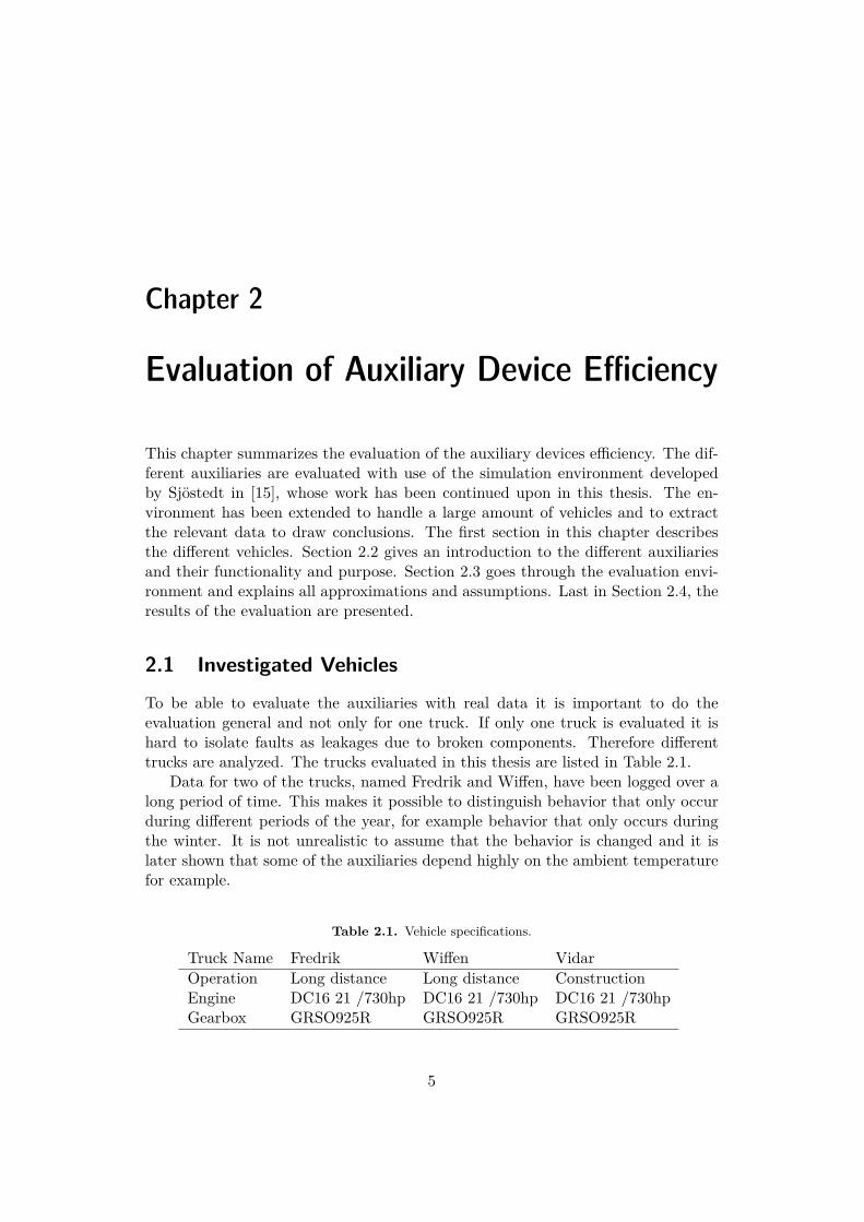
To be able to evaluate the auxiliaries with real data it is important to do theevaluation general and not only for one truck. If only one truck is evaluated it ishard to isolate faults as leakages due to broken components. Therefore differenttrucks are analyzed. The trucks evaluated in this thesis are listed in Table 2.1.
Data for two of the trucks, named Fredrik and Wiffen, have been logged over along period of time. This makes it possible to distinguish behavior that only occurduring different periods of the year, for example behavior that only occurs duringthe winter. It is not unrealistic to assume that the behavior is changed and it islater shown that some of the auxiliaries depend highly on the ambient temperaturefor example.
Table 2.1. Vehicle specifications.
Truck Name Fredrik Wiffen VidarOperation Long distance Long distance ConstructionEngine DC16 21 /730hp DC16 21 /730hp DC16 21 /730hpGearbox GRSO925R GRSO925R GRSO925R
5

CHAPTER 2. EVALUATION OF AUXILIARY DEVICE EFFICIENCY
There also exists data, which have been collected from a third truck referred to asVidar. The amount of data available is not over the same long period, but can beused to evaluate and confirm the behavior of the other trucks.
2.2 Auxiliary DevicesThe following section will give a brief introduction to the different auxiliary systemsinvolved in this thesis. An auxiliary is defined as a device that is connected andpowered by the engine, but not directly used for the propulsion of the vehicle.However, most auxiliaries are completely necessary to be able to drive the vehicle.
The auxiliaries are either connected to the engine with cog or with belt. Some ofthe auxiliaries are connected with clutches, thus making them controllable. Otherauxiliaries have energy storage, as for example the air compressor which can buildup extra pressure in the air system. The auxiliaries and their connection to theengine can be seen in Figure 2.1. Beneath the figure, a more detailed description ofthe different auxiliary devices can be found.
Engine Be
lt
Co
g
Alternator
Water pump
AC compressor
Cooling fan
Air compressor
Oil pump
Power steering pump On/off clutch
Viscous clutch
Figure 2.1. The different auxiliaries examined in this thesis and their connec-tion to the engine. Two of the auxiliaries are clutched, the air compressor isalso controllable with a power saving function.
2.2.1 Air Compressor
The compressed air in the pneumatic system is used for many different componentssuch as brakes, parking brake and suspension. For buses, compressed air is alsoused for opening the doors and for kneeling. For buses driving in city traffic, theair compressor is one of the largest energy consumers. Investigations regardinguse of electrical components instead of pneumatic components have been examined
6
2.2. AUXILIARY DEVICES
because of the low efficiency of compressed air. The energy consumption of thecompressor is increased due to leakages and the need to remove vapor from thecompressed air to prevent the brakes from freezing.
The air pressure system also uses an energy saving function. When the energy isfree, i.e when the vehicle brakes, the air pressure system is charged with a pressureslightly higher than normal. This function could be applied to the other auxiliaries,but for now, most of them lack any kind of energy storage.
2.2.2 Oil Pump
The oil pump is directly attached to the engine. Therefore, the energy consumptionof the pump is proportional to the engine speed of the vehicle. The purpose of theoil system is to lubricate the engine. Without the oil pump, the engine would seizeup immediately. It is therefore of great importance that the oil pump is robustlydesigned and able to lubricate at all times.
2.2.3 Power Steering Pump
The power steering system is used to give additional torque to the driver’s steeringwheel movements. The power steering pump is directly connected to the enginewith cog wheels which leads to energy losses when the power steering is not used.A combined hydraulic electric system is investigated in [7]. An electrical systemmakes it possible to electronically control the steering of the vehicle which enablesautonomous features such as collision avoidance or lane keeping assistance [15].With the recent interest in such applications, it is likely that the power steering willbe electrically or semi-electrically controlled in the near future.
2.2.4 Alternator
The purpose of the alternator is to charge the batteries in the 24 V electrical powersystem. The alternator is connected to the engine with a belt. The efficiency ofthe currently used alternator is not sufficient to power other auxiliaries electrically.With a power system with higher voltage, it would most likely be beneficial to useelectrically controlled auxiliaries since this gives precise control and the problemwith overpowering is easily handled with simple control strategies.
For hybrid trucks, it is also necessary for some of the auxiliaries to be electricallydriven. When the vehicle is powered with electricity and the combustion engine isturned off, it would be impossible to maneuver the vehicle since the combustionengine would not provide power to the steering pump [15]. The trend today istowards more electronically controlled vehicles. Thus, it is likely that the alternatorwill be more efficient with electrical driven auxiliaries in the future.
7

CHAPTER 2. EVALUATION OF AUXILIARY DEVICE EFFICIENCY
2.2.5 Coolant Pump
The purpose of the coolant system is to prevent components from overheating. Thecoolant system is mainly used to cool the combustion engine, but is also used tocool other components such as the air compressor and the retarder. The coolantpump is connected to the engine with a belt. With the fixed connection, the speedof the pump and the flow of the coolant is proportional to the engine speed. Sincethe cooling system needs to be able to cool the components at all times, the pump isdesigned to provide sufficient cooling at all speeds. Due to the proportionality, thepump provides unnecessary cooling at higher speeds and therefore energy is wasted.
When designing the coolant system, there are different paths to take regardingengine temperature. One way is to let the temperature in the engine vary, whichmeans that the cooling fan can be used less. The other path is to let the engine runat a high temperature, thus making the combustion efficient. However, to be ableto run the engine at a high temperature, a good and fast cooling system is needed.One solution could be to control the cooling system with an electrical pump, thusmaking it possible to control the flow of coolant and the engine temperature withbetter precision.
2.2.6 Cooling Fan
The purpose of the cooling fan is to cool the coolant flowing through the radiator.The fan is controlled with a viscous clutch, which is partly controlled depending onthe temperature of the engine. The fan is often disengaged but when it is engaged,the cooling fan is one of the largest energy consumers.
The decision algorithm for the fan control is rather complex. This is due to themany different component that can request cooling by the cooling system. Exceptthe engine, components such as the retarder, the air compressor and the gearboxcan request fan and cooling. Therefore, it is not trivial to investigate why thefan is engaged without knowing all the requests from the different components.Nevertheless, the main and most important component that requests fan cooling isthe engine.
2.2.7 AC Compressor
The air condition provides cooling for the driver’s cabin. The AC compressor isconnected to the engine with a belt with an on/off clutch. Since the AC is connectedwith a clutch it would be possible to turn the AC off completely. Turning the ACoff will not affect the performance of the vehicle, though it will affect the comfortof the driver. Thus, there is a decision that has to be made between comfort andpotential fuel savings.
8

2.3. MATLAB/SIMULINK SIMULATION ENVIRONMENT
Figure 2.2. Basic idea in [15] for modeling the consumption of the auxiliaries.Each auxiliary device is modeled differently, but use input variables such asengine and fan speed. From the inputs, the models outputs the torque and thepower that is consumed by each auxiliary.
2.3 MATLAB/Simulink Simulation Environment
The energy consumption of the auxiliary devices is examined in MATLAB/Simulinkwith use of the work by [15], which has been extended in this thesis. With the aux-iliaries connected to the engine, they will add negative torque to the engine. Sincethe power consumption of all auxiliaries can not be measured directly, the powerconsumption is modeled. The basic idea of the modeling can be seen in Figure 2.2.Inputs to the model are logged signals from vehicles who use a logging system calledMlog. Mlog is a system which is used to get feedback and gather data from heavy-duty vehicles operating on real roads. The signals can be logged with differentsampling rates, however a sampling rate of 10 Hz is most common. Examples of theMlog signals that are used as inputs to the auxiliary model are engine rotationalspeed, cooling fan rotational speed and control signals for the auxiliaries. The out-puts of the models are torque and power, given for each of the auxiliaries. Thetorque and power consumption can then be evaluated for each driving cycle, forexample to investigate how the auxiliary devices behave during an uphill slope. Forheavy-duty vehicles it is important to have much power available when it is needed,for example in a uphill slope. It is also interesting to investigate the auxiliariesduring a longer period of time. By doing this, the average consumption of eachauxiliary can be evaluated and compared against the other auxiliaries. It is alsopossible to compare the power consumption against ambient variables such as theoutdoor temperature. As an example, it is reasonable to assume that the powerconsumption of the AC compressor should have a strong correlation to the ambienttemperature.
In the following subsection, the modeling of the auxiliaries will be further ex-plained. This is followed by a short conclusion regarding approximations and as-sumptions made in the models. For more detailed information about the models,please refer to [15].
9

CHAPTER 2. EVALUATION OF AUXILIARY DEVICE EFFICIENCY
2.3.1 Model StructureThe power for mechanical rotational systems is in general calculated as
P = τ · ω (2.1)
where τ is the torque and ω is angular velocity. By using the well known rela-tions ω=2πf and f=nrpm
60 , where nrpm is revolutions per minute, the power can beobtained as
P = τ · π30 · nrpm. (2.2)
This calculation is done for each of the auxiliaries.Some of the auxiliaries, such as the oil, steer and coolant pump, are modeled
with look-up tables where the inputs are signals from the Mlog system. For theoil pump, the look-up table transforms engine speed and oil temperature to torque.Similar for the steering pump, the torque is given from the engine speed and thepressure in the power steering system. For the coolant pump, the torque is directlygiven from the engine speed. Further, the air compressor is modeled with a look-uptable depending on the status and pressure in the system, as well as the enginespeed. Both the AC-compressor and the cooling fan are connected with clutches.The torque of the AC is modeled with a look-up table depending on the engine speedand the status of the clutch. The fan is the only auxiliary modeled mathematically.The input to the fan model is the rotational speed of the fan. The torque of thecooling fan is given by
τfan = k · n2fan ·GUF · 10−6 (2.3)
where k is the fan constant and nfan is the rotational speed of the fan. GUF is thegear up factor which appears if the fan has an external driving belt for additionalcooling, otherwise it is set to one.
2.3.2 Approximations and AssumptionsSome of the look-up tables depend on variables that can not be measured. There-fore, those variables must be modeled. Sjöstedt approached this problem just bysetting the variables to appropriate constants. The constants are chosen accordingto corresponding data sheets. The complexity of modeling some of the variableswould be to much for this project but could easily be included if there would beneed for a more precise evaluation. The accuracy of the models are though stillhigh and the data is very valuable since it can illustrate behavior that can not beseen in for example test rigs.
2.4 Auxiliary Device EfficiencyThis section summarize the results of the investigation of the power consumptionof the auxiliary devices. First, the power consumptions of the auxiliary devices arelisted. Second, the dependencies on variables such as ambient temperature and roadinclination are discussed. Last, the results are summarized in a concluding section.
10

2.4. AUXILIARY DEVICE EFFICIENCY
Table 2.2. Average mean, maximum, minimum energy consumption with the stan-dard deviation. The time active, i.e. the amount of time connected to the engine,is also shown. The values can be compared to the maximum total engine power at540 kW.
Auxiliary Device Mean [kW] Max [kW] Std [kW] Time ActiveCompressor 1.50 10.0 1.47 11.4 %1
Oil pump 2.15 6.01 0.83 100 %Coolant pump 1.62 6.25 0.70 100 %Cooling fan 0.83 17.9 1.67 17.2 %Alternator 1.52 2.71 0.37 100 %AC compressor 0.73 5.07 1.29 19.0 %Power steering pump 0.85 1.95 0.24 100 %
2.4.1 Consumption
As mentioned, the vehicles investigated in this thesis do all have 16 liter, 730hp,V8-engines, which equals a maximum power output of approximately 540 kW. Itis rather well known according to previous investigations that the average powerconsumption of each auxiliary is around 1 kW. With seven auxiliaries, the averagepower consumption of the devices would equal approximately 7 kW, or about 1 %of the maximum total engine power. However, it will be shown that during someperiods, the power consumption of the auxiliaries can reach much higher values.
To start the investigation, the average power consumption of the auxiliaries forthe vehicle Fredrik is summarized in Table 2.2. The average mean consumption isshown together with the average maximum value and the average standard devia-tion. It can be seen that the power consumption differs significantly between thedevices. The differences between the mean and maximum values are largest for theclutched auxiliaries which could be expected. It is reasonable to assume that this isthe reason why clutches were introduced. Remember that the clutched auxiliariesare the cooling fan and the AC compressor. The air compressor has an energy sav-ing function, which also leads to a more variated power consumption as the mean,max and standard deviation for the air compressor shows.
The two auxiliaries that consume the largest amount of energy are the oil pumpand the coolant pump. It would be interesting to make these pumps variable tobe able to control the flows with higher precision and get rid of the overpowering.This would likely lower the energy consumption of the pumps. However, both thesedevices have very high demands on robustness. If these systems fail, the engine andother components seize up immediately.
For the auxiliaries connected with a clutch, i.e. auxiliaries that can be controlled,it is interesting to examine the amount of time that they are connected to the engine.It can be seen that the fan and the AC compressor spend less than 20 % of the total
1Duration spent while not in power saving mode.
11

CHAPTER 2. EVALUATION OF AUXILIARY DEVICE EFFICIENCY
time active. Also, as mentioned, the air compressor has an energy saving functionwhich utilizes free energy when the vehicle brakes. When braking, the air pressuresystem is pushed to a slightly higher pressure than normal. The time active for theair compressor corresponds to the time when not in power saving mode.
One can also investigate separate driving cycles independently to find how theauxiliaries behave for example during uphill slopes. It will soon be shown that theconsumption of the auxiliaries highly depends on the characteristics of the road.A typical scenario when the auxiliary power consumption is high can be seen inFigure 2.3. The uphill slope is very steep and the vehicle climb approximately300 m during 400 seconds. It is a demanding climb and it can be seen that theengine speed is almost at 2000 rpm and the engine utilizes full engine power duringmost of the road segment. The dips in power correspond to gear changes whichalso affects the engine speed. The total power of the auxiliaries is also shown in thefigure. It can be seen that the average consumption for the auxiliaries at the roadsegment is above 20 kW. At maximum, the consumption reaches around 50 kWwhich now is about 10 % of the total engine power. During the climb, the powershould be used to propel the vehicle. A loss of 20-50 kW to the auxiliaries is asignificant power loss, very noticeable to the driver.
It is interesting that the driving cycles when the power consumption of theauxiliaries are high, often are the same routes. More specific for Fredrik, mostof the vehicle’s routes are in Norway, which is good for examining how the vehiclebehaves in a varying topological environment. How the power consumption dependson the incline of the road, together with the ambient temperature, the engine speed,and the velocity of the vehicle is further discussed in the next section.
2.4.2 Dependencies
Temperature dependence
As can be expected, the power consumption of the different auxiliaries depend onthe ambient temperature. There are mainly two auxiliaries that show ambienttemperature dependence; the AC compressor and the air compressor. The ACcompressor which is connected with a clutch, can and should be disengaged whenthe ambient temperature is low and there is no need for cooling. In Figure 2.4, thetemperature dependence for the vehicle Fredrik is shown. The data is logged forcycles over almost a year, starting in June 2012 to February 2013. The figure showsthe mean temperature plotted against the mean power consumption. It is clearlyseen that the AC does not consume any energy at lower temperatures. However,it is noticeable that the AC is used for temperatures around 5-15 ◦C which isquestionable since it should not be any need of cooling. During this interval, 27 %of the cycles have a mean power consumption above 50 W. 13 % of the cycleshave a power consumption above 200 W and about 6 % of the cycles have a powerconsumption above 400 W. If it would be possible to not use the AC during thesetemperatures energy could be saved.
12

2.4. AUXILIARY DEVICE EFFICIENCY
−200 −150 −100 −50 0 50 100 150 200010002000
Time [s]
rpm
Engine speed
−200 −150 −100 −50 0 50 100 150 200−300−200−100
0100
Time [s]
mAltitude
−200 −150 −100 −50 0 50 100 150 2000200400600
Time [s]
kW
Total engine power
−200 −150 −100 −50 0 50 100 150 2000204060
Time [s]
kW
Total auxiliary power
−200 −150 −100 −50 0 50 100 150 200010203040
Time [s]
kW
Fan power
−200 −150 −100 −50 0 50 100 150 20005
101520
Time [s]
kW
Compressor power
Figure 2.3. A typical scenario when the auxiliaries consumes a large amount ofenergy. The vehicle needs to utilize maximum engine power during most parts ofthe uphill. Since the rotational speed of the engine is high combined with that thecooling fan and the compressor are used simultaneously, the power consumption ofthe auxiliaries equals 20-50 kW which corresponds to a power loss of 10 %.
13

CHAPTER 2. EVALUATION OF AUXILIARY DEVICE EFFICIENCY
−15 −10 −5 0 5 10 15 20 25 300
0.5
1
1.5
2
2.5
3
Temperature [◦C]
AC
power
[kW
]
Figure 2.4. The temperature dependence for the AC compressor. The areaaround 5-15 ◦C is of interest since there should not be any need of AC coolingduring these temperatures. Yet, the power consumption in this interval is above50 W during 27 % of the cycles, above 200 W during 13 % of the cycles andabove 400 W for about 6 % of the cycles.
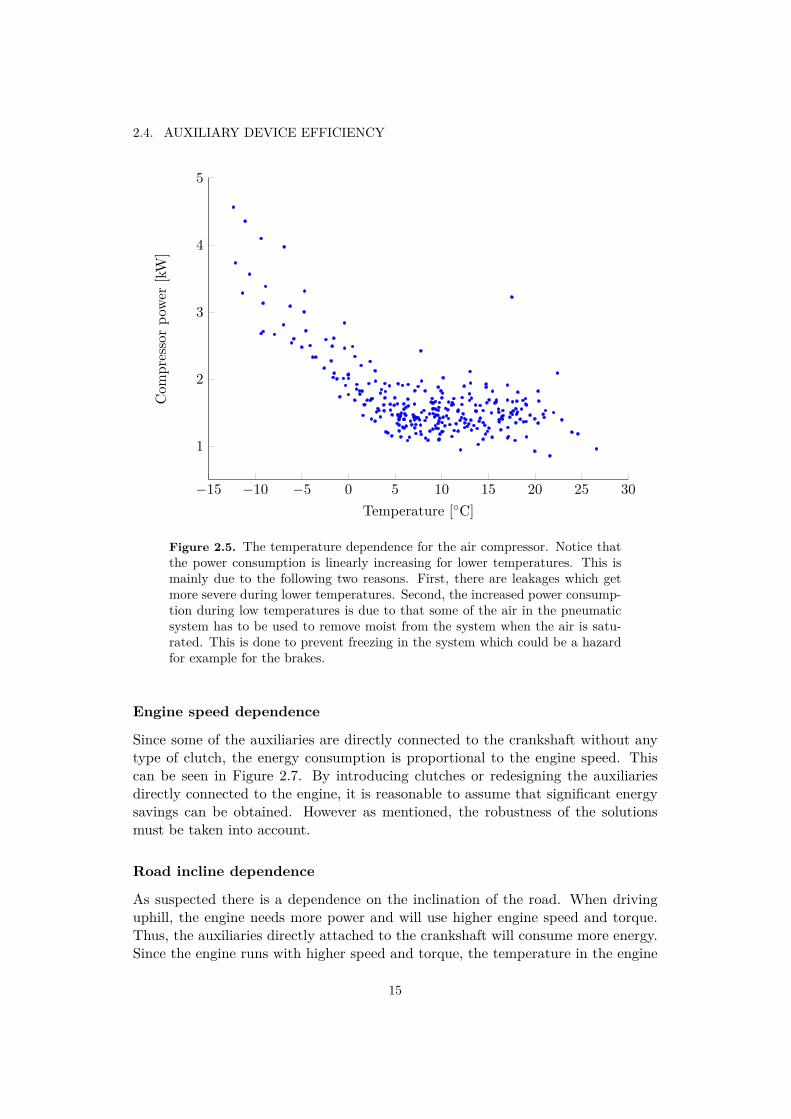
There is also a temperature dependence for the air compressor. In opposite to theAC compressor, the air compressor consumes more energy during low temperatures.This can be seen in Figure 2.5. The higher consumption of the air compressor ispartly caused by leakages, but also due to the need to remove moist air to preventfreezing.
Vehicle speed dependence
The cooling fan shows a dependence on the traveling speed of the vehicle. At highspeed, the fan is engaged more seldom. This is due to the air flow from the airintake which is enough to provide sufficiently low coolant temperature. This can beseen in Figure 2.6. If we disregard the small dependence of the cooling fan, there areno auxiliaries that show dependence directly to the speed of the vehicle. However,the speed of the vehicle depends for example both on the engine speed and the roadincline, which will be discussed next.
14
2.4. AUXILIARY DEVICE EFFICIENCY
−15 −10 −5 0 5 10 15 20 25 30
1
2
3
4
5
Temperature [◦C]
Com
pressorpo
wer
[kW
]
Figure 2.5. The temperature dependence for the air compressor. Notice thatthe power consumption is linearly increasing for lower temperatures. This ismainly due to the following two reasons. First, there are leakages which getmore severe during lower temperatures. Second, the increased power consump-tion during low temperatures is due to that some of the air in the pneumaticsystem has to be used to remove moist from the system when the air is satu-rated. This is done to prevent freezing in the system which could be a hazardfor example for the brakes.
Engine speed dependence
Since some of the auxiliaries are directly connected to the crankshaft without anytype of clutch, the energy consumption is proportional to the engine speed. Thiscan be seen in Figure 2.7. By introducing clutches or redesigning the auxiliariesdirectly connected to the engine, it is reasonable to assume that significant energysavings can be obtained. However as mentioned, the robustness of the solutionsmust be taken into account.
Road incline dependence
As suspected there is a dependence on the inclination of the road. When drivinguphill, the engine needs more power and will use higher engine speed and torque.Thus, the auxiliaries directly attached to the crankshaft will consume more energy.Since the engine runs with higher speed and torque, the temperature in the engine
15

CHAPTER 2. EVALUATION OF AUXILIARY DEVICE EFFICIENCY
30 40 50 60 70 80 90 1000
0.5
1
1.5
2
2.5
3
3.5
Vehicle speed [km/h]
Fanpo
wer
[kW
]
Figure 2.6. The average fan power dependence on the average speed of thevehicle. During high vehicle speeds the air intake is sufficient to alone coolthe coolant in the radiator. Since the fan is clutched it can be disengaged andtherefore the power consumption is lowered. Notice the low power consumptionfor speeds above 70 km/h.
will also increase. Therefore, more cooling is needed. At high engine speed it islikely that the auxiliaries will be overpowered and therefore it will be a loss of energywhen the power is needed to get the vehicle up the hill. When driving downhill, theengine brake and the retarder are active. The retarder also generates heat whichneeds to be cooled. Since the coolant pump can not be activated or controlled, thetemperature will increase and the cooling fan must be activated. The fan consumesa large amount of energy when activated and as seen, the fan is one of the largestconsumers of energy when active.
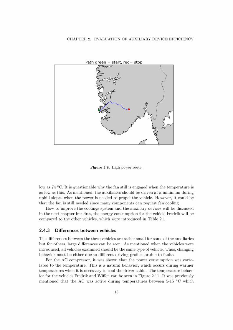
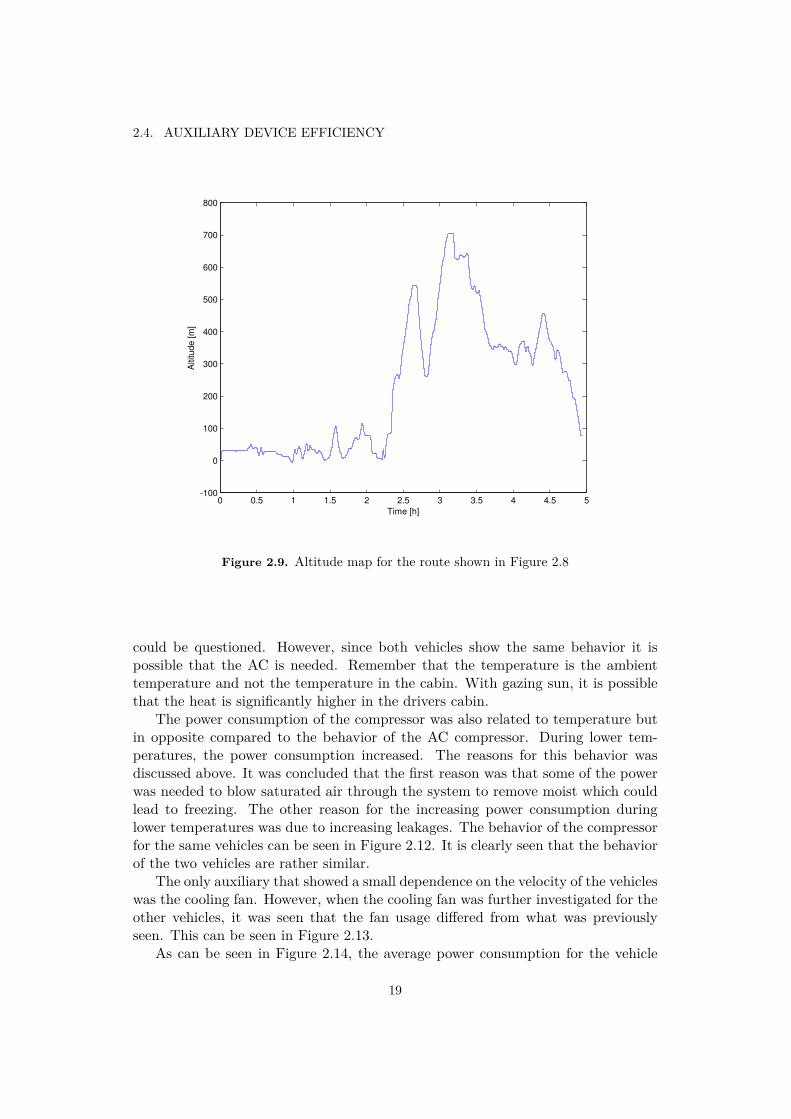
It is interesting to investigate during which road inclines the energy consumptionof the auxiliaries are high. When the total consumption of the auxiliaries are large,it is often caused due to the cooling fan. However, when the total consumption ishigh during a longer period of time, we often have the same incline dependence. Itis either steep uphill, or steep downhill, the fan is engaged either way. This hill isalso often the same and it is a part of the route shown in Figure 2.8. This route inNorway is between the city of Haugesund and the small village of Seljord. The routeis demanding due to its large variation in altitude, which can be seen in Figure 2.9.
16

2.4. AUXILIARY DEVICE EFFICIENCY
700 800 900 1000 1100 1200 1300 14000.5
1
1.5
2
2.5C
oola
nt pum
p p
ow
er
[kW
]
Engine Speed [rpm]
700 800 900 1000 1100 1200 1300 14001
1.5
2
2.5
3
Oil
pum
p p
ow
er
[kW
]
Engine Speed [rpm]
Figure 2.7. The proportional behavior due to the connection to the enginewithout any type of clutch. The figure shows the average consumption for theoil and coolant pump. It would be of interest to add a clutch to lower the powerconsumption during higher rotational speeds to get rid of the overpowering andthus save energy.
That the fan is activated downhill is not a problem, since the engine torque will mostlikely be negative and thus no torque is needed from the engine. This means that thefan will not have an impact on the fuel consumption. The main reason that the fanis engaged is most likely that it needs to lower the temperature of the coolant whichtakes up heat from the retarder. The retarder is a braking system which generatesheat when used. The oil temperature in the retarder can reach up to 180 ◦C whichneeds to be cooled [3]. Also, by activating the fan, some extra negative torque willbe added to the crankshaft, which will only help with the braking of the truck.
It is more critical to the fuel consumption that the fan is engaged during uphillclimbs. In Figure 2.10 the behavior for the engine temperature and fan speed canbe seen. The purpose of the fan is to cool the engine. Fan cooling is requested at95 ◦C which can be seen. The fan is then also engaged and it can be seen that therotational speed of the fan increases and that the engine cools off. However, withthe increasing fan speed, the power consumption of the fan also increases which canbe seen in Figure 2.3. The temperature in the engine is at the end of the interval as
17
CHAPTER 2. EVALUATION OF AUXILIARY DEVICE EFFICIENCY
Figure 2.8. High power route.
low as 74 ◦C. It is questionable why the fan still is engaged when the temperature isas low as this. As mentioned, the auxiliaries should be driven at a minimum duringuphill slopes when the power is needed to propel the vehicle. However, it could bethat the fan is still needed since many components can request fan cooling.
How to improve the coolings system and the auxiliary devices will be discussedin the next chapter but first, the energy consumption for the vehicle Fredrik will becompared to the other vehicles, which were introduced in Table 2.1.
2.4.3 Differences between vehiclesThe differences between the three vehicles are rather small for some of the auxiliariesbut for others, large differences can be seen. As mentioned when the vehicles wereintroduced, all vehicles examined should be the same type of vehicle. Thus, changingbehavior must be either due to different driving profiles or due to faults.
For the AC compressor, it was shown that the power consumption was corre-lated to the temperature. This is a natural behavior, which occurs during warmertemperatures when it is necessary to cool the driver cabin. The temperature behav-ior for the vehicles Fredrik and Wiffen can be seen in Figure 2.11. It was previouslymentioned that the AC was active during temperatures between 5-15 ◦C which
18
2.4. AUXILIARY DEVICE EFFICIENCY
0 0.5 1 1.5 2 2.5 3 3.5 4 4.5 5-100
0
100
200
300
400
500
600
700
800
Time [h]
Altitude [m
]
Figure 2.9. Altitude map for the route shown in Figure 2.8
could be questioned. However, since both vehicles show the same behavior it ispossible that the AC is needed. Remember that the temperature is the ambienttemperature and not the temperature in the cabin. With gazing sun, it is possiblethat the heat is significantly higher in the drivers cabin.
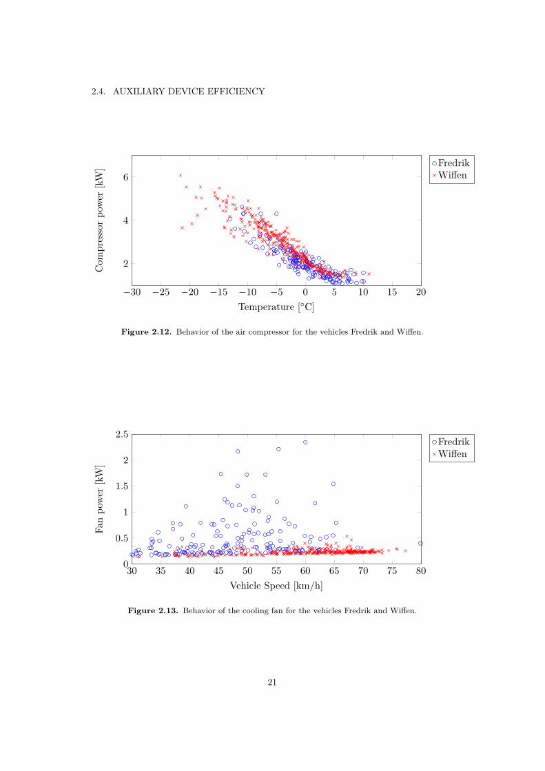
The power consumption of the compressor was also related to temperature butin opposite compared to the behavior of the AC compressor. During lower tem-peratures, the power consumption increased. The reasons for this behavior wasdiscussed above. It was concluded that the first reason was that some of the powerwas needed to blow saturated air through the system to remove moist which couldlead to freezing. The other reason for the increasing power consumption duringlower temperatures was due to increasing leakages. The behavior of the compressorfor the same vehicles can be seen in Figure 2.12. It is clearly seen that the behaviorof the two vehicles are rather similar.
The only auxiliary that showed a small dependence on the velocity of the vehicleswas the cooling fan. However, when the cooling fan was further investigated for theother vehicles, it was seen that the fan usage differed from what was previouslyseen. This can be seen in Figure 2.13.
As can be seen in Figure 2.14, the average power consumption for the vehicle
19

CHAPTER 2. EVALUATION OF AUXILIARY DEVICE EFFICIENCY
−200 −150 −100 −50 0 50 100 150 200708090
100
Time [s]
◦ C
Engine Temperature
−200 −150 −100 −50 0 50 100 150 200010002000
Time [s]
rpm
Fan Speed
Figure 2.10. Engine temperature and fan speed for the road segment illustrated inFigure 2.3.
−30 −25 −20 −15 −10 −5 0 5 10 15 200
0.1
0.2
0.3
0.4
Temperature [◦C]
AC
power
[kW
]
FredrikWiffen
Figure 2.11. Differences for the AC compressor between the vehicles Fredrik andWiffen.
20
2.4. AUXILIARY DEVICE EFFICIENCY
−30 −25 −20 −15 −10 −5 0 5 10 15 20
2
4
6
Temperature [◦C]
Com
pressorpo
wer
[kW
] FredrikWiffen
Figure 2.12. Behavior of the air compressor for the vehicles Fredrik and Wiffen.
30 35 40 45 50 55 60 65 70 75 800
0.5
1
1.5
2
2.5
Vehicle Speed [km/h]
Fanpo
wer
[kW
]
FredrikWiffen
Figure 2.13. Behavior of the cooling fan for the vehicles Fredrik and Wiffen.
21

CHAPTER 2. EVALUATION OF AUXILIARY DEVICE EFFICIENCY
250 500 750 1000 1250 1500 1750 20000
20
40
60
80
100
Mean fan power [W]
Amou
ntof
cycles
[%]
FredrikWiffen
Figure 2.14. Power consumption of the cooling fan for Fredrik and Wiffen. Thevehicle Wiffen uses less fan than the vehicle Fredrik. This is probably due to thatFredrik operates in an environment with a more varying topology.
Wiffen is almost never above 0.5 kW. The reason for this is not known, but it isprobably due to the driving profile of the vehicle. It was shown that Fredrik oftenwas used in Norway, with largely changing topology. Where Wiffen operates is notexactly known since the vehicle does not have GPS available. However, it is knownthat Wiffen operates in Sweden between the cities of Östersund and Borlänge. Itcould be the case that the environment where Fredrik operates is more strenuous.To investigate this further, the velocity, the engine speed, the torque, and the roadinclination are compared between the vehicles.
It is hinted in Figure 2.13 that the vehicle Wiffen often travels with highervelocity than Fredrik and actually, the average speed for Wiffen for the whole periodis around 61km/h, while for Fredrik the average speed is around 48 km/h. However,the energy consumption of the fan differs independently of speed. It could thoughbe the case that Wiffen travels on more open road for example highways and thusis able to keep higher velocity.
For engine speed and torque, the average values are approximately the same.However, the mean does not say anything about the variations. During highwaycruising, the torque and the engine speed are at levels where there is no need to usethe fan. The need to use the fan only occurs during aggressive driving. Therefore, itis better to look at the standard deviations. The standard deviations for the enginetorque are approximately the same for both vehicles. But for the engine speed, itis 260 rpm for Wiffen and 300 rpm for Fredrik.
Last, the road inclination. The mean standard deviation for the road inclinetaken for all cycles is roughly 2.1 % for Wiffen and 3.2 % for Fredrik. Combining
22
2.4. AUXILIARY DEVICE EFFICIENCY
30 35 40 45 50 55 60 65 70 75 800
0.5
1
1.5
Vehicle Speed [km/h]
Fanpo
wer
[kW
]
FredrikWiffenVidar
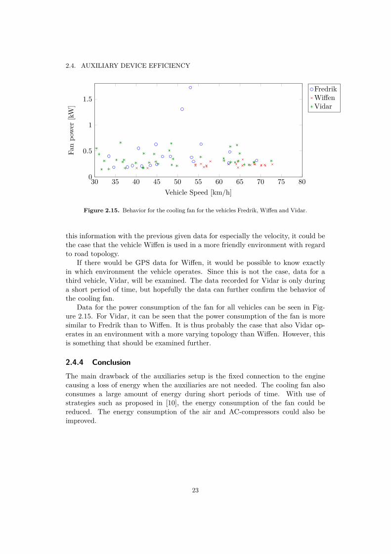
Figure 2.15. Behavior for the cooling fan for the vehicles Fredrik, Wiffen and Vidar.
this information with the previous given data for especially the velocity, it could bethe case that the vehicle Wiffen is used in a more friendly environment with regardto road topology.
If there would be GPS data for Wiffen, it would be possible to know exactlyin which environment the vehicle operates. Since this is not the case, data for athird vehicle, Vidar, will be examined. The data recorded for Vidar is only duringa short period of time, but hopefully the data can further confirm the behavior ofthe cooling fan.
Data for the power consumption of the fan for all vehicles can be seen in Fig-ure 2.15. For Vidar, it can be seen that the power consumption of the fan is moresimilar to Fredrik than to Wiffen. It is thus probably the case that also Vidar op-erates in an environment with a more varying topology than Wiffen. However, thisis something that should be examined further.
2.4.4 ConclusionThe main drawback of the auxiliaries setup is the fixed connection to the enginecausing a loss of energy when the auxiliaries are not needed. The cooling fan alsoconsumes a large amount of energy during short periods of time. With use ofstrategies such as proposed in [10], the energy consumption of the fan could bereduced. The energy consumption of the air and AC-compressors could also beimproved.
23

Chapter 3
Potential Improvements of AuxiliaryDevice Structure and Efficiency
There are different ways to improve the efficiency of the auxiliaries. In this chapter,ideas of how this could be done are evaluated. First, in Section 3.1, the mainstrategies for controlling auxiliary devices are shown. The potential benefits of eachstrategy is evaluated and compared against the other strategies. In Section 3.2, aconclusion is drawn regarding which strategy that would be most beneficial withrespect to cost, time and feasibility to investigate further in this thesis.
3.1 Strategies
3.1.1 Conventional Auxiliaries
With the auxiliary setup used in Scania trucks today, which is described in Sec-tion 2.2, it is quite challenging to increase the efficiency and reduce the energyconsumption of the auxiliaries. Since the auxiliaries often are connected directlyto the crankshaft, their energy consumption can not be reduced without alteringthe hardware or reducing the rotational speed of the engine. However, there arestill improvements that can be done. For the auxiliaries already designed with dif-ferent type of clutches, different strategies could be applied to either reduce thetotal fuel consumption, or increase the performance of the truck by disabling theauxiliaries during for example hill climbing. Disabling the auxiliaries during uphillclimbs would yield more power to drive the vehicle forward since no negative torquefrom the auxiliaries would be applied to the crankshaft. To be able to reduce theconsumption or provide more power momentarily, it would probably be required touse sensor data and information about the surrounding environment such as theroad topology. With use of this information, it can be decided when it is suitableand optimal to power the auxiliaries.
25

CHAPTER 3. POTENTIAL IMPROVEMENTS OF AUXILIARY DEVICESTRUCTURE AND EFFICIENCY
Driving Modes
Modern cars comes with different driving modes e.g. performance mode, where thevehicle is optimized to provide as much power as possible to the engine drive. Inperformance mode, fuel consumption is not of concern. Compared to performancemode, there is likely also an economical mode, where the fuel consumption is of mostimportance. This should also be used for the auxiliaries in heavy-duty vehicles.
In long-haulage companies, the drivers are often rewarded for economical drivingwith different kind of bonuses. If the driver is able to turn different auxiliaries offand remove luxuries such as air conditioning, the total fuel consumption woulddecrease. Performance mode would most likely be used when there is need of extraengine power. According to the investigation in Section 2.4, just turning off the ACwould yield approximately 1 kW additional drive power. Since the AC only affectsthe driver and not the performance of the vehicle, the effects of not having it on isnot that dangerous. Applying this strategy to more important auxiliaries such asthe cooling fan would require carefully designed control algorithms.
If this strategy of not having the auxiliaries connected at the same time could beapplied, it would be possible to reduce the maximum consumed torque and power.This would make it possible to reduce the size of the engine. With a reduced enginesize the vehicle weighs less and in the engine room there is more room for othercomponents, i.e. a larger and more efficient alternator.
There have also been investigations on how to control the engine temperature tokeep the engine as efficient as possible. One strategy is to keep the temperature ashigh as possible, which leads to a more effective combustion process. The drawbackwith a higher engine temperature is that the safety margin decreases. If the tem-perature reaches values that are to high, it is likely that the engine will break, whichmust be avoided. This puts pressure on the cooling system and the expenses for itwould probably increase. The other strategy is to let the temperature in the enginevary as proposed in [10]. The combustion is not always as efficient but according toprevious work, the auxiliaries consume less energy. These two strategies should beevaluated and compared to each other to see which of them that decrease the totalfuel consumption of the engine. It would be possible that one want to use thesestrategies depending on the performance mode, for example having a high enginetemperature in performance mode and letting the temperature vary in economicalmode.
Reduced Fuel Consumption
It is a hard problem to reduce the total fuel consumption without altering the hard-ware setup which exists today. The most likely strategy that could be applied forthis purpose is to use large amounts of input sensor data to the control algorithms.This data could be look-ahead information about the upcoming road, the amountof throttle applied, gear, if the brakes are active and different temperatures such asambient, cabin and engine temperature. With many inputs available it would be
26

3.1. STRATEGIES
possible to combine them all in an overall optimal controlled system. The objectiveof the control system could either be to minimize the fuel consumption or optimizethe power from the engine, giving the vehicle much power, for example when goinguphill.
The strategy for the air compressor could also be applied to other auxiliaries.This strategy stores extra energy when the vehicle brakes, taking advantage of freeenergy and saving it for later. The main problem with applying this strategy toother auxiliaries is the lack of energy storage. An alternative could be to introducea flywheel which is loaded with mechanical energy or a generator which loads abattery during braking. The stored energy can then be used by the auxiliaries orutilized when extra power is needed, during for example acceleration.
3.1.2 Electrical Auxiliaries
The most likely future scenario for the auxiliaries is that they will be electricallydriven to some extent. With electrical systems it is possible to get rid of overpow-ering and the auxiliaries can be precisely controlled for good efficiency. The mainproblem with electrical auxiliaries is the lack of power in the 24 V electrical system.The electrical system in todays vehicles is not sufficient to power the different aux-iliaries. Also, another problem is that the efficiency of the alternator is low whichmeans that there will be loss of energy.
In hybrid vehicles it would be possible to power the auxiliaries with electricityconverted with a DC/DC converter from the high voltage system. It is also anecessity for hybrid vehicles that the auxiliaries such as the steering pump is poweredelectrically so the maneuverability of the vehicle is not lost when the combustionengine is turned off. For mild hybrid vehicles, i.e. vehicles with a low voltage powersystem such as 48 V, it would also be possible to power the auxiliaries electrically.However, when redesigning the auxiliaries both safety and uptime robustness haveto be of concern.
It would also be possible to recover energy from the brakes or from waste heat.Waste heat from the exhausts could for example be converted to electricity with athermoelectric generator [15].
The possibilities and simplicity of storing energy electrically is also somethingthat speaks for electrical auxiliaries. With a generator with high efficiency anda power system sufficient to power the auxiliaries, electrical auxiliaries would bepreferred. However, there are still issues regarding the robustness of electrical solu-tions.
3.1.3 Hybrid Auxiliaries
One other solution would be the use of hybrid auxiliaries. With hybrid auxiliaries,the auxiliaries can be connected with a clutch. When the electrical system is suf-ficient to power the auxiliaries, they remain clutched and no mechanical power istaken from the engine. When the electrical power is not sufficient, mechanical en-
27

CHAPTER 3. POTENTIAL IMPROVEMENTS OF AUXILIARY DEVICESTRUCTURE AND EFFICIENCY
ergy is used. Methods like these are already investigated and one example is theelectro/hydraulic steering servo in [7]. That the steering servo is investigated is dueto the need of being able to maneuver the vehicle when the combustion engine isturned off, but also to be able to electronically control the steering for applicationssuch as lane keeping assistance and collision avoidance.
3.2 ConclusionThere are different solutions for controlling the auxiliaries and they all have pros andcons. The future will most likely involve electrical auxiliaries, but their introductionwill lead to extensive redesign of the whole engine setup and high developmentcosts. The introduction of electrically driven auxiliaries will come naturally duringthe launch of hybrid and electrical vehicles. Also, the energy savings of the newdesigns have to be larger than the cost for introducing new sensors or componentsin the vehicles. Therefore, the continued work in this thesis will examine a controlstrategy to decrease the energy consumption of the auxiliaries without altering theirhardware.
28

Chapter 4
Optimal Control of the Cooling System
This chapter examines a control strategy for an adaptive look-ahead cruise controllerwhere the cooling system is included. It is assumed that the road topology is knownfor the whole road segment within the look-ahead horizon. In the first section of thischapter, the purpose of the optimization problem is explained. Furthermore, modelsfor the vehicle and cooling system dynamics are derived. The derived cooling systemmodel is tuned against recorded Mlog data to match the behavior of the system in areal truck. After this, the optimization problem is mathematically formulated andlast the simulation procedure with the optimization algorithm is described.
4.1 Look-Ahead Optimization
An ordinary cruise controller regulates the velocity to a desired reference speedwhich is often constant. Recently, these controllers have become more adaptive,i.e. they regulate the velocity depending on for example the inclination of the roador the surrounding traffic. Adaptive cruise controllers simplify the work of thedrivers, but could also reduce the fuel consumption of the vehicle by for examplechoosing the optimal velocity and gear, with regard to fuel consumption. However,the adaptive cruise controller often operates independently of other systems suchas the cooling system and the effects of these systems on the optimal solution arerather unknown. Since it was shown earlier that the cooling system consumes alarge amount of energy, as well as the system is crucial for the engine and vehicleto function, the cooling system is a good candidate for further investigation.
The purpose of the optimal control problem is to find the optimal control strat-egy to go from one point to another, while minimizing the consumed fuel andtraveled time. The optimal control problem decides optimal cooling fan controlcombined with optimal velocity and optimal gear choice. Both the temperatureand the velocity are constrained between feasible values. If the temperature wouldreach too high values, the engine could seize up. For the velocity, it is obvious thatthere are speed limits that must be kept.
It is important to understand how the cooling system influences the optimal
29

CHAPTER 4. OPTIMAL CONTROL OF THE COOLING SYSTEM
solution. In heavy-duty vehicles, the available cooling is sometimes limited, whichcould lead to that the torque of the engine must be limited so the engine doesnot overheat. If the cooling system and engine control could be integrated andcombined, these kind of problems could be solved automatically with a real-timeoptimization algorithm.
4.2 ModelingIn the following section, a model for the dynamics of the truck and the coolingsystem is derived. The model is derived with a complexity suitable to the followingoptimization problem. Since the complexity of the optimal solution increases withthe number of states, only three states are chosen for the complete system.
4.2.1 Vehicle Dynamics
The dynamical model of the longitudinal motion of the truck is based on [9], whichis also used in [6], [8] and [13]. In Figure 4.1, the powertrain of a truck is shown.
Figure 4.1. Powertrain of the modeled truck, illustrated as in [13]. The powerfrom the engine is transfered to the auxiliaries and to the clutch.
30

4.2. MODELING
The dynamics of the engine can be described as
Jeωe = τe − τaux − τfric − τc (4.1)
where Je is the mass moment of inertia of the engine, we is the angular velocityof the engine, τe is the driving torque from the combustion, τaux is the torqueconsumed by the auxiliaries, τfric is the torque loss due to friction and τc is thetorque transfered to the clutch. The driving torque of the engine can be describedas
τe = fe(ωe, uf ) (4.2)where fe is function depending on the fuel flow uf into the engine and the rotationalspeed ωe of the engine. However, by defining a feasible region with a maximumengine torque depending on the rotational speed of the engine, it is assumed thatthere exists a feasible control signal that can provide the desired engine torque.Furthermore, the torque transmitted to the wheel is given by
τw = iητc (4.3)
where i is the conversion ratio between the clutch and the wheel and η is a constantwhich models energy losses. The relation between the angular velocities of theengine and the wheel is given by
ωe = iωw. (4.4)
The dynamic motion of the wheel is then described by
Jlωw = τw − τb − rwFw (4.5)
where Jl is the inertia of the wheel which also includes the inertia of the clutch,propeller shaft and driveshaft. τb corresponds to the braking torque and rwFw isthe resulting torque due to the friction force Fw. The longitudinal motion of thetruck can be described by
mdv
dt= Fw − Fa(v)− Fr(α)− Fg(α) (4.6)
where m and v are the mass and the velocity of the truck. The force Fa is due toair drag, Fr is due to the rolling resistance and Fg is the force on the truck causedby gravity. The forces are described in Table 4.1. The velocity of the truck is givenby
v = rwωw (4.7)where rw is the radius of the wheel.
The given equations can then be combined. Starting with replacing the angularvelocities with use of Equation (4.3), (4.4) and (4.7), it is found that
Jldv
dt=rω(iητc − τb − rwFw) (4.8)
Jedv
dt=rω
i(τe − τaux − τfric − τc). (4.9)
31

CHAPTER 4. OPTIMAL CONTROL OF THE COOLING SYSTEM
Force Explanation ExpressionFa(v) Air drag 1
2cwAaρav2
Fr(α) Rolling resistance mgcr cos(α)Fg(α) Gravitational force mg sin(α)
Table 4.1. Repulsive forces described as in [6].
Furthermore, combining these two equation by replacing τc and solving for Fω givesus
Fω = 1rω
(iη(τe − τfric − τaux)− τb)−1r2
ω
(ηi2Je + Jl)dv
dt. (4.10)
By finally replacing Fω in equation (4.6), the dynamics of the vehicle is summarizedas
dv
dt= rw
Jl +mr2w + ηi2Je
(iη(τe − τfric − τaux)
− τb − rw(Fa(v)− Fr(α)− Fg(α))). (4.11)
4.2.2 Fuel ConsumptionThe mass flow of fuel is given by
dmf
dt= 1ηdieselEdiesel
τeωe (4.12)
where ηdiesel and Ediesel are the combustion efficiency of diesel and the amount ofenergy per kilogram diesel. There are several ways of computing the fueling andthis is one of two methods proposed in [13], where a fuel map is the alternativeapproach. A large fuel map gives a detailed description of the fueling and it takesnonlinearities into account. Thus, when exact values for the fueling is needed, theuse of the fuel map is preferred. A typical fuel map can be seen in Figure 4.2.
The simplicity of Equation (4.12) makes the function a suitable choice when theexact amounts of fueling is not of highest interest. Calculating the fuel consumptionwith use of Equation (4.12) instead of using the fuel map has been proven to becalculation and time efficient, thus in this thesis the equation will be used for thefuel consumption. The differences of the outcome of the two methods are also shownin [13]. Even though there are some minor differences between using the map andthe function, the differences are small and therefore disregarded.
4.2.3 Modeling of the Cooling SystemIn the following subsection, a model for the cooling system is derived. The dynamicsare based on heat flows and temperature balance. The model is also evaluated inthe next subsection and compared to Mlog-data. The model for the cooling system
32

4.2. MODELING
Figure 4.2. An example fuel map.
is taken from [16] and further simplified to become suitable for the optimal controlproblem. The dynamics of the cooling system is described by
dT
dt= γ1Qin − γ2Qout. (4.13)
Here T is the temperature of the coolant. The change of temperature depends onthe heat flows Qin and Qout, which are the heat flows in and out from the coolant.The two parameters γ1 and γ2 are constants calibrated to fit the cooling systembehavior according to Mlog-data. It is further assumed that the heat flows into thecoolant are all governed from the combustion in the engine and from the retarderwhile braking. Thus,
Qin = Qeng +Qret (4.14)
whereQeng = mexhcexh(β1Texh − β2T ). (4.15)
Here, cexh is the heat capacity of the exhausts. Furthermore, mexh and Texh are theexhaust mass flow and the exhaust temperature, which are given by approximatedsecond order functions depending on the torque and rotational speed of the engine.These functions have been fitted with the method of least squares to measured data
33

CHAPTER 4. OPTIMAL CONTROL OF THE COOLING SYSTEM
maps, similar to the one for the fueling in Figure 4.2. The two parameters β1 andβ2 are once again constants calibrated to fit the coolant system behavior accordingto Mlog-data.
For the retarder, it is assumed that all braking energy is transformed to heatinto the coolant. The braking energy is the braking power over time, therefore themomentary heat from the retarder equals
Qret = τb · ωe (4.16)
and it is assumed that the retarder is placed on an axis which rotates with the samespeed as the engine.
Furthermore, it is assumed that all heat out from the coolant is transferedthrough the radiator. The heat flow out of the radiator is given by
Qout = f(mair, mcool)(T − Tair) (4.17)
where f(mair, mcool) is a function depending on the air mass flow and the coolantmass flow into the radiator. The air mass flow is calculated from the air volumeflow into the front of the truck times the density of the air. Thus,
mair = Vairρair. (4.18)
The air volume flow depends on the speed of the vehicle and the rotational speedof the fan. The volume flow is calculated as
Vair = a1ω2fan + a2ωfan + a3vvehicle + a4 (4.19)
where a1, a2, a3 and a4 are constants. Further, ρair is given by
ρair = pair
R(Tair + Tabs) (4.20)
where pair is the ambient pressure, R is the gas constant, and Tair + Tabs is theambient temperature in Kelvin.
The coolant mass flow is assumed to be proportional to the speed of the engine,therefore
mcool = cNωeng (4.21)
and our model for the coolant temperature is finished.The torque needed to rotate the fan is given above in Section 2.3 as
τfan = k · ω2fan · 106. (4.22)
4.2.4 Model ValidationThe modeling of the heat into the coolant Qin is a bit to approximative. First, theheat from the combustion does not go into the coolant directly. Between the coolantand the combustion zone there is an inner engine block. This inner engine block
34
4.2. MODELING
0 100 200 300 400 500 600 700 80080
90
100
Time [s]
Tempe
rature
[◦C] Model
Mlog
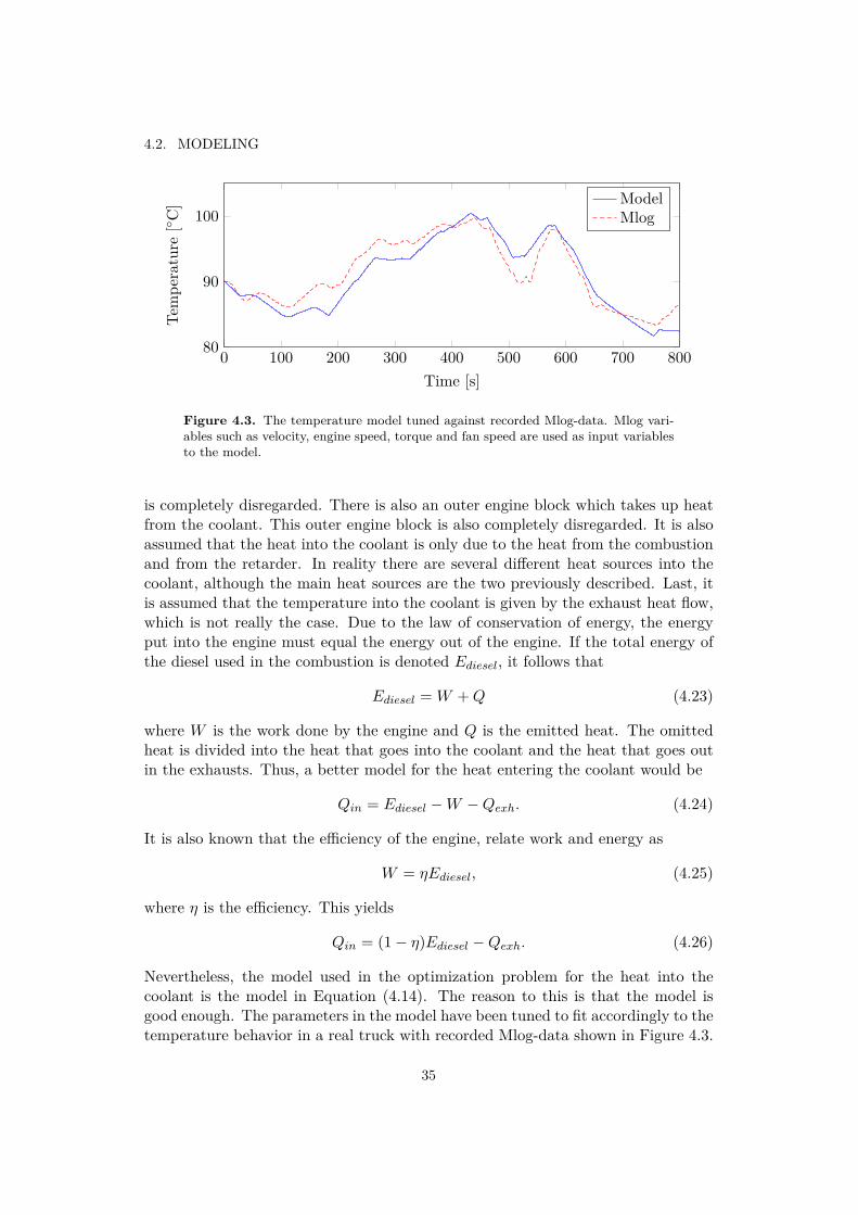
Figure 4.3. The temperature model tuned against recorded Mlog-data. Mlog vari-ables such as velocity, engine speed, torque and fan speed are used as input variablesto the model.
is completely disregarded. There is also an outer engine block which takes up heatfrom the coolant. This outer engine block is also completely disregarded. It is alsoassumed that the heat into the coolant is only due to the heat from the combustionand from the retarder. In reality there are several different heat sources into thecoolant, although the main heat sources are the two previously described. Last, itis assumed that the temperature into the coolant is given by the exhaust heat flow,which is not really the case. Due to the law of conservation of energy, the energyput into the engine must equal the energy out of the engine. If the total energy ofthe diesel used in the combustion is denoted Ediesel, it follows that
Ediesel = W +Q (4.23)
where W is the work done by the engine and Q is the emitted heat. The omittedheat is divided into the heat that goes into the coolant and the heat that goes outin the exhausts. Thus, a better model for the heat entering the coolant would be
Qin = Ediesel −W −Qexh. (4.24)
It is also known that the efficiency of the engine, relate work and energy as
W = ηEdiesel, (4.25)
where η is the efficiency. This yields
Qin = (1− η)Ediesel −Qexh. (4.26)
Nevertheless, the model used in the optimization problem for the heat into thecoolant is the model in Equation (4.14). The reason to this is that the model isgood enough. The parameters in the model have been tuned to fit accordingly to thetemperature behavior in a real truck with recorded Mlog-data shown in Figure 4.3.
35
CHAPTER 4. OPTIMAL CONTROL OF THE COOLING SYSTEM
0 50 100 150 200 250 300 350 400
85
90
95
Time [s]
Tempe
rature
[◦C]
ModelMlog
Figure 4.4. The temperature model validated against real recorded Mlog-data. Thetemperature model illustrates the main characteristics of the real system but it isclearly seen that the model could be improved. One of the main reasons that thetemperature model fails to describe the real system is because the thermostat whichregulates the coolant flow is not included.
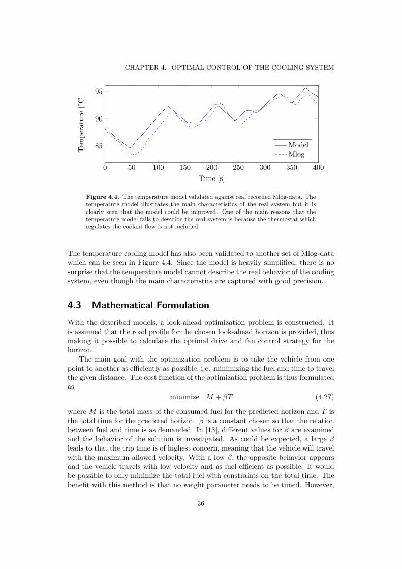
The temperature cooling model has also been validated to another set of Mlog-datawhich can be seen in Figure 4.4. Since the model is heavily simplified, there is nosurprise that the temperature model cannot describe the real behavior of the coolingsystem, even though the main characteristics are captured with good precision.
4.3 Mathematical FormulationWith the described models, a look-ahead optimization problem is constructed. Itis assumed that the road profile for the chosen look-ahead horizon is provided, thusmaking it possible to calculate the optimal drive and fan control strategy for thehorizon.
The main goal with the optimization problem is to take the vehicle from onepoint to another as efficiently as possible, i.e. minimizing the fuel and time to travelthe given distance. The cost function of the optimization problem is thus formulatedas
minimize M + βT (4.27)
where M is the total mass of the consumed fuel for the predicted horizon and T isthe total time for the predicted horizon. β is a constant chosen so that the relationbetween fuel and time is as demanded. In [13], different values for β are examinedand the behavior of the solution is investigated. As could be expected, a large βleads to that the trip time is of highest concern, meaning that the vehicle will travelwith the maximum allowed velocity. With a low β, the opposite behavior appearsand the vehicle travels with low velocity and as fuel efficient as possible. It wouldbe possible to only minimize the total fuel with constraints on the total time. Thebenefit with this method is that no weight parameter needs to be tuned. However,
36

4.3. MATHEMATICAL FORMULATION
it would be required to introduce a new state for time, which leads to that thecomplexity for solving the problem increases [12].
The given cost function should now be minimized with regard to the above vehi-cle and cooling system dynamics given in Section 4.2. The dynamics are formulatedin position instead of time and according to [6], it is beneficial to formulate thedynamics with energy instead of velocity to avoid oscillating solutions. With use ofthe chain rule it is found that
dv
dt= dv
ds
ds
dt= v
dv
ds. (4.28)
Furthermoredv2
ds= 2vdv
ds= 2dv
dt. (4.29)
For the temperature, it is straightforward that
dT
dt= dT
ds
ds
dt= v
dT
ds. (4.30)
The dynamics are also discretized with a sampling distance h with use of EulerForward. The discretized dynamics for each step k are summarized to
v2k+1 = v2
k + 2hdvdt
Tk+1 = Tk + h
v
dT
dt(4.31)
gk+1 = gk + f(gk)
which finally leads to
v2k+1 = v2
k + 2hrw
Jl +mr2w + ηi2Je
(iη(τe − τfric − τfan)
− τb − rw(Fa(v)− Fr(α)− Fg(α)))
(4.32)
Tk+1 = Tk + h
v
(γ1Qin − γ2Qout
)gk+1 = gk + f(gk)
where f(gk) is a function describing which gear changes that are allowed from thecurrent gear. From neutral gear, we are allowed to change the gear arbitrarily.Neutral can also be reached from any gear. Otherwise it is only allowed to shift onegear up or one gear down. Only one gear change is allowed each step.
There are also different constraints on the problem. To start with, we havelimitations on the engine torque and rotational speed. As mentioned, the maxi-mum engine torque τmax, is defined by the rotational speed and the fuel input asdescribed when Equation (4.2) was introduced. The engine torque is bounded bythis maximum value. The rotational speed of the engine is also bounded by ωmax.
37
CHAPTER 4. OPTIMAL CONTROL OF THE COOLING SYSTEM
Since the fan is assumed to be directly connected to the engine by the clutch withoutgearing2, the speed of the fan cannot be larger than the speed of the engine. Hence,the inequality constraints for the engine torque and for the rotational speeds of theengine and the fan are
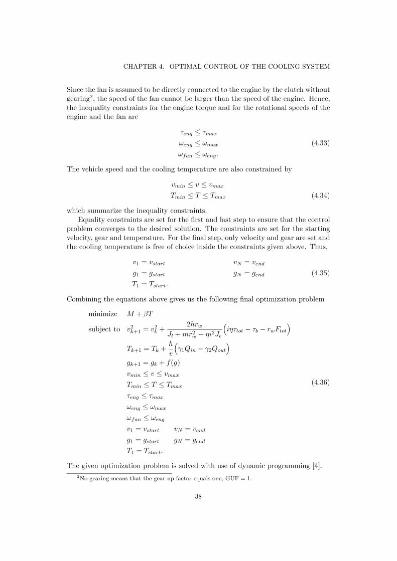
τeng ≤ τmax
ωeng ≤ ωmax (4.33)ωfan ≤ ωeng.
The vehicle speed and the cooling temperature are also constrained by
vmin ≤ v ≤ vmax
Tmin ≤ T ≤ Tmax (4.34)
which summarize the inequality constraints.Equality constraints are set for the first and last step to ensure that the control
problem converges to the desired solution. The constraints are set for the startingvelocity, gear and temperature. For the final step, only velocity and gear are set andthe cooling temperature is free of choice inside the constraints given above. Thus,
v1 = vstart vN = vend
g1 = gstart gN = gend (4.35)T1 = Tstart.
Combining the equations above gives us the following final optimization problem
minimize M + βT
subject to v2k+1 = v2
k + 2hrw
Jl +mr2w + ηi2Je
(iητtot − τb − rwFtot
)Tk+1 = Tk + h
v
(γ1Qin − γ2Qout
)gk+1 = gk + f(g)vmin ≤ v ≤ vmax
Tmin ≤ T ≤ Tmax
τeng ≤ τmax
ωeng ≤ ωmax
ωfan ≤ ωeng
v1 = vstart vN = vend
g1 = gstart gN = gend
T1 = Tstart.
(4.36)
The given optimization problem is solved with use of dynamic programming [4].2No gearing means that the gear up factor equals one, GUF = 1.
38

4.4. SIMULATION
4.4 SimulationThe standard dynamic programming algorithm is stated in [6] as
1. Let JN (x) = 0 x ∈ SN
2. Let k = N − 1
3. Let Jk(x) = minu∈Uk
{ξk(x, u) + Jk+1(f(x, u))} x ∈ Sk
4. Repeat (3) for k = N − 2, N − 3, . . . , 0
5. The optimal cost is J0 and the sought control vector is the optimal controlfrom the initial state to the final state.
In the standard dynamical programming algorithm, each possible control vectorthat takes the system to another state is calculated. Therefore, the number ofcalculations increase exponentially with the number of controls and steps. Hence,the number of calculations grows fast and the problem will quickly become too largeto handle. If the states and the controls are quantized, the complexity is reducedand grows quadratically with the number of states and controls. However, withquantized controls, there is no guarantee to end up at a quantized state and thusthere will be need to interpolate.
An alternative approach is taken in [6]. Here the state space is fixed and thecontrol vector for taking one state to the next is calculated. With this method,the number of calculations is bounded by the number of states and steps and thecalculations increase quadratically with the states and linearly with the steps. Withthe alternative approach, only the states are quantized and there is no need ofinterpolation. The alternative dynamic programming algorithm used for solvingthe optimization problem is formulated as
1. Let JN (xN ) = 0 xN ∈ SN
2. Let k = N − 1
3. Let Jk(xi) = minxj∈Sk+1
{ξi,jk + Jk+1(xj)} xi ∈ Sk
4. Repeat (3) for k = N − 2, N − 3, . . . , 0
5. The optimal cost is J0 and the sought control vector is the optimal controlfrom the initial state to the final state.
The optimization problem is solved with use of the work conducted by [13] inMatlab. As mentioned the cooling system has been introduced so the solver has beenmodified with regards to this. Different road profiles are built before simulations.An example road can be seen in Figure 4.5.
39
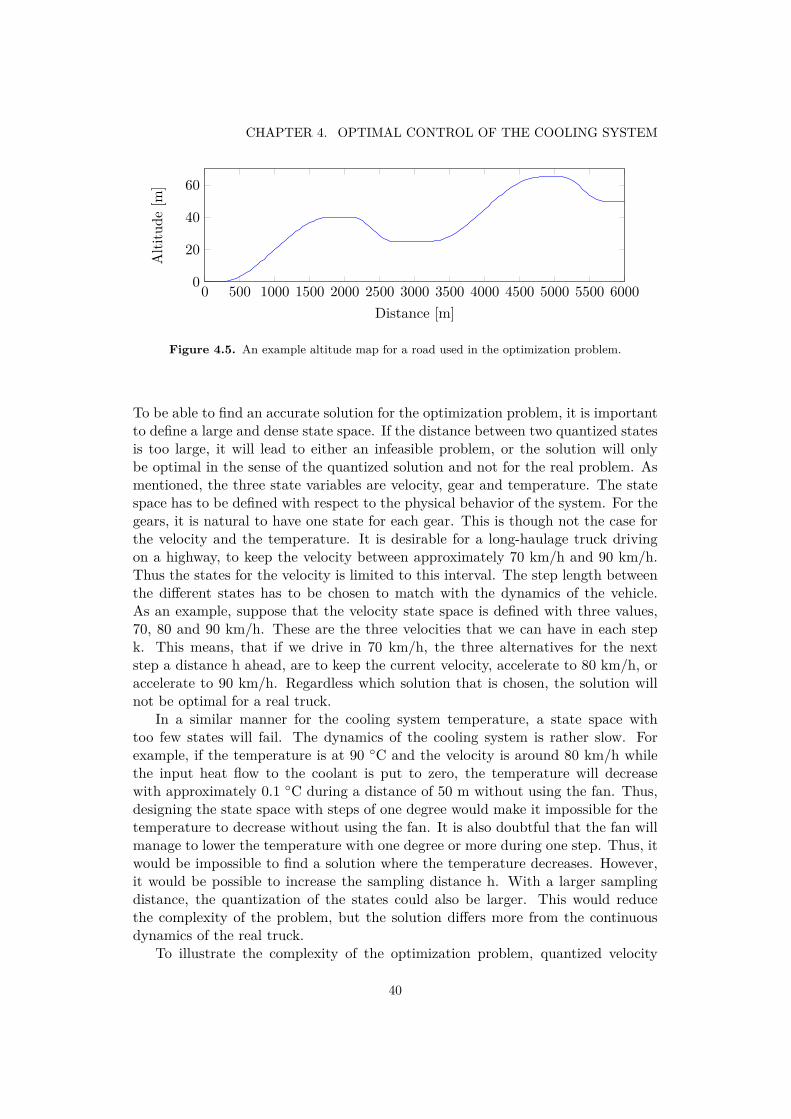
CHAPTER 4. OPTIMAL CONTROL OF THE COOLING SYSTEM
0 500 1000 1500 2000 2500 3000 3500 4000 4500 5000 5500 60000
20
40
60
Distance [m]
Altitude
[m]
Figure 4.5. An example altitude map for a road used in the optimization problem.
To be able to find an accurate solution for the optimization problem, it is importantto define a large and dense state space. If the distance between two quantized statesis too large, it will lead to either an infeasible problem, or the solution will onlybe optimal in the sense of the quantized solution and not for the real problem. Asmentioned, the three state variables are velocity, gear and temperature. The statespace has to be defined with respect to the physical behavior of the system. For thegears, it is natural to have one state for each gear. This is though not the case forthe velocity and the temperature. It is desirable for a long-haulage truck drivingon a highway, to keep the velocity between approximately 70 km/h and 90 km/h.Thus the states for the velocity is limited to this interval. The step length betweenthe different states has to be chosen to match with the dynamics of the vehicle.As an example, suppose that the velocity state space is defined with three values,70, 80 and 90 km/h. These are the three velocities that we can have in each stepk. This means, that if we drive in 70 km/h, the three alternatives for the nextstep a distance h ahead, are to keep the current velocity, accelerate to 80 km/h, oraccelerate to 90 km/h. Regardless which solution that is chosen, the solution willnot be optimal for a real truck.
In a similar manner for the cooling system temperature, a state space withtoo few states will fail. The dynamics of the cooling system is rather slow. Forexample, if the temperature is at 90 ◦C and the velocity is around 80 km/h whilethe input heat flow to the coolant is put to zero, the temperature will decreasewith approximately 0.1 ◦C during a distance of 50 m without using the fan. Thus,designing the state space with steps of one degree would make it impossible for thetemperature to decrease without using the fan. It is also doubtful that the fan willmanage to lower the temperature with one degree or more during one step. Thus, itwould be impossible to find a solution where the temperature decreases. However,it would be possible to increase the sampling distance h. With a larger samplingdistance, the quantization of the states could also be larger. This would reducethe complexity of the problem, but the solution differs more from the continuousdynamics of the real truck.
To illustrate the complexity of the optimization problem, quantized velocity
40

4.4. SIMULATION
steps of 0.2 km/h and quantized temperature steps of 0.05 ◦C are chosen. If thestate space for velocity and temperature is limited between 70-90 km/h and 70-100 ◦C, this would lead to 100 × 600 states for velocity and temperature. If wealso add 4 gears and optimize over 10 steps, the number of calculations will bearound 6 · 1011. This amount of calculations will take much time. Therefore, to geta realistic computational time, the state space or the search space must be limited.The dynamics of the system shows how the system behave and therefore calculationsthat are clearly unfeasible, such as changing the temperature more than 1 ◦C canbe skipped. The search space is defined similar to [6], both for the gears, velocityand temperature. The search space for the gears has been described above. For thevelocity, the search space is defined differently depending on the slope of the roadwhile for the temperature, a difference of ±0.1 ◦C is allowed. The search space hasto be defined with care. If the search space is to coarse, the optimal solution couldbe changed since the most optimal solution is never calculated. However, with thesearch space defined, it has been found that the calculation time for solving theoptimal control problem is reduced to almost half.
The search space and other improvements for the simulations are further dis-cussed in the final concluding chapter. In the following chapter, the outcome of theoptimization for different setups and road profiles will be shown.
41

Chapter 5
Results
In the following chapter the results of the optimal control problem will be shown.The solution will show the optimal gear and velocity choice for the vehicle as wellas the optimal temperature of the cooling system and the optimal fan speed. Thesampling distance h is set to 50 m for all solutions. The optimal solution will beshown for different starting temperatures which will display the effects of the coolingsystem. In the next and final chapter, the results will be evaluated and conclusionsthereof will be drawn.
5.1 Basic Road Profiles
The optimal control solution will first be shown for two different drive cases; downhillroad and uphill road. This is mainly to illustrate that the system dynamics behavesas expected, but also to illustrate the main characteristics of the optimal solutionfor simple problems. After the basic problems, the control problem will be evaluatedfor a mixed road which includes both downhill and uphill slopes. Here, the solutionof the optimization problems when the cooling system is and is not included will becompared. As stated in the problem description in the beginning of the thesis, it isinteresting to know if the auxiliary devices influence the optimal driving strategy.If this is true, the control of the auxiliaries should be taken into account when forexample smart adaptive cruise controllers are designed.
5.1.1 Uphill Road
The uphill road used in simulation is a 2000 m road with a slope of length 1600 mand 3 % angle. The optimal solution for the uphill road segment can be seenin Figure 5.1. Here, three solutions are shown which all have different startingtemperatures. The starting temperatures and the optimal temperature and fanspeed trajectories can be seen in Figure 5.2. It can be seen that the temperatureis increasing when the engine power is high up the hill. By comparing the figures,it can be seen that the temperature of the cooling system affects the desired gear
43

CHAPTER 5. RESULTS
0 200 400 600 800 1000 1200 1400 1600 1800 200060708090
100
Distance [m]
km/h
Velocity
0 200 400 600 800 1000 1200 1400 1600 1800 200002040
Distance [m]
Altitude
Altitude
0 200 400 600 800 1000 1200 1400 1600 1800 2000910111213
Distance [m]
Gearnr
Gear
0 200 400 600 800 1000 1200 1400 1600 1800 200001000200030004000
Distance [m]
Nm
Torque
0 200 400 600 800 1000 1200 1400 1600 1800 2000100012001400160018002000
Distance [m]
rpm
Engine Speed
Figure 5.1. Optimal solution for an uphill slope where the vehicle accelerates beforethe start of the slope. The solution that use lowest gear and highest rotational speedis the solution where the temperature in the cooling system is the highest.
44
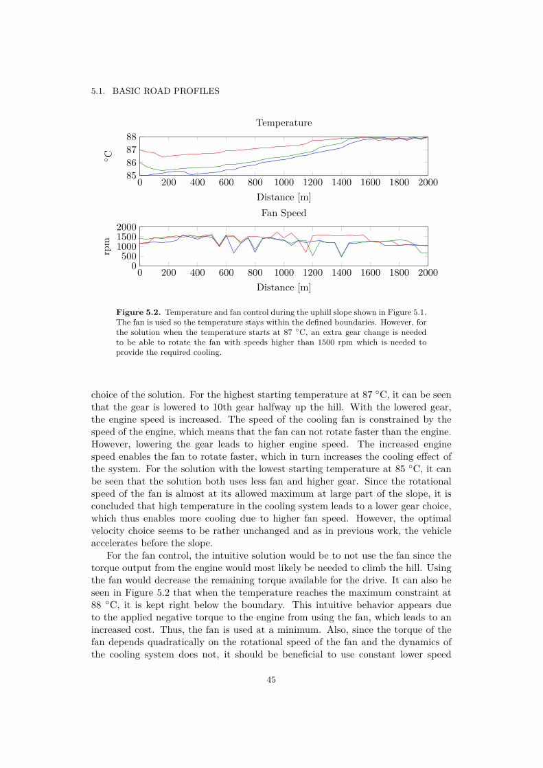
5.1. BASIC ROAD PROFILES
0 200 400 600 800 1000 1200 1400 1600 1800 200085868788
Distance [m]
◦ CTemperature
0 200 400 600 800 1000 1200 1400 1600 1800 20000500
100015002000
Distance [m]
rpm
Fan Speed
Figure 5.2. Temperature and fan control during the uphill slope shown in Figure 5.1.The fan is used so the temperature stays within the defined boundaries. However, forthe solution when the temperature starts at 87 ◦C, an extra gear change is neededto be able to rotate the fan with speeds higher than 1500 rpm which is needed toprovide the required cooling.
choice of the solution. For the highest starting temperature at 87 ◦C, it can be seenthat the gear is lowered to 10th gear halfway up the hill. With the lowered gear,the engine speed is increased. The speed of the cooling fan is constrained by thespeed of the engine, which means that the fan can not rotate faster than the engine.However, lowering the gear leads to higher engine speed. The increased enginespeed enables the fan to rotate faster, which in turn increases the cooling effect ofthe system. For the solution with the lowest starting temperature at 85 ◦C, it canbe seen that the solution both uses less fan and higher gear. Since the rotationalspeed of the fan is almost at its allowed maximum at large part of the slope, it isconcluded that high temperature in the cooling system leads to a lower gear choice,which thus enables more cooling due to higher fan speed. However, the optimalvelocity choice seems to be rather unchanged and as in previous work, the vehicleaccelerates before the slope.
For the fan control, the intuitive solution would be to not use the fan since thetorque output from the engine would most likely be needed to climb the hill. Usingthe fan would decrease the remaining torque available for the drive. It can also beseen in Figure 5.2 that when the temperature reaches the maximum constraint at88 ◦C, it is kept right below the boundary. This intuitive behavior appears dueto the applied negative torque to the engine from using the fan, which leads to anincreased cost. Thus, the fan is used at a minimum. Also, since the torque of thefan depends quadratically on the rotational speed of the fan and the dynamics ofthe cooling system does not, it should be beneficial to use constant lower speed
45

CHAPTER 5. RESULTS
instead of for example bang-bang control where the rotational speed of the fan isswitched between maximum speed and zero speed.
5.1.2 Downhill RoadThe downhill road used in simulation is a 2000 m road with a slope of length 1600 mand angle -3 %. Three solutions for the optimal control problem when the startingtemperature is varied can be seen in Figure 5.3. There are some interesting remarks.First as seen in previous work, the vehicle lowers the velocity while it approachesthe downhill. For the whole downhill segment, the torque is less than or equal tozero for all solutions and hence the vehicle is not propelled by the engine and nofuel is consumed. The velocity of the vehicle is kept between the constrained limitsbut reaches the upper limit in the middle of the slope. Therefore some braking withthe retarder is needed.
The temperature for the solutions can be seen in Figure 5.4. At approximately700 m, the retarder brakes which leads to the increasing temperature. It can also beseen that the fan is engaged during most of the downhill. However, in Figure 5.3 itwas seen that the engine torque was negative with a gear engaged for all solutions.Therefore, using the fan has no effect on the fuel consumption and the fan is thusused as an extra engine brake.
5.2 Mixed Road ProfileThe optimal solution will now be evaluated for the example road shown in Figure 4.5and the optimal solution can be seen in Figure 5.5. The road consists of two uphillsand two downhills. The uphills are 1600 m with an incline of 3 % and the downhillsare 600 m with an incline of -2 %. The figure illustrates four different solutions,where the first three solutions are for different starting temperatures which canbe seen in Figure 5.6. The fourth dashed solution however, is when the coolingsystem is completely disregarded. It can clearly be seen that the solution whenthe cooling system is disregarded differs significantly from the other solutions. Themain difference is that the vehicle does not eco-roll [1], i.e. go to neutral gear, withthe cooling system.
It can be seen that the vehicle eco-rolls for the first time at approximately2000 m. In Figure 5.6, it can be seen that at this point, the temperature is aroundthe maximum constraint. It is an interesting remark that the vehicle does not eco-roll when the cooling system is included. This could be due to several reasons.First, since the temperature is at the maximum constraint, the engine needs to becooled. Going to eco-roll limits the rotational speed of the fan to 500 rpm whichis the engine speed during eco-roll. With the fan rotating with only 500 rpm, itcould be that this amount of cooling is not sufficient to bring the temperature to theminimum before the next uphill. Therefore, the fan would need to be engaged moreduring the uphill and thus, eco-roll is not chosen. The second alternative whichmight be more likely, is that the velocity is too low to make eco-roll beneficial. It
46

5.2. MIXED ROAD PROFILE
0 200 400 600 800 1000 1200 1400 1600 1800 20007075808590
Distance [m]
km/h
Velocity
0 200 400 600 800 1000 1200 1400 1600 1800 20000204060
Distance [m]
Altitude
Altitude
0 200 400 600 800 1000 1200 1400 1600 1800 200011
12
13
Distance [m]
Gearnr
Gear
0 200 400 600 800 1000 1200 1400 1600 1800 2000−2000−1000
01000
Distance [m]
Nm
Torque
0 200 400 600 800 1000 1200 1400 1600 1800 20001100120013001400
Distance [m]
rpm
Engine Speed
Figure 5.3. Optimal solution for a downhill slope where the vehicle slow downbefore the crest. The fuel consumption for the road is around zero for all solutions.The temperature for the solutions can be seen in Figure 5.4.
47
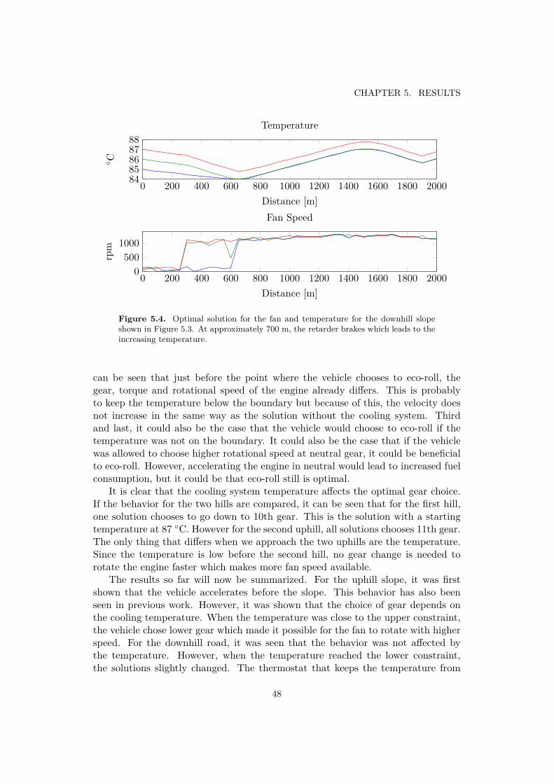
CHAPTER 5. RESULTS
0 200 400 600 800 1000 1200 1400 1600 1800 20008485868788
Distance [m]
◦ CTemperature
0 200 400 600 800 1000 1200 1400 1600 1800 20000500
1000
Distance [m]
rpm
Fan Speed
Figure 5.4. Optimal solution for the fan and temperature for the downhill slopeshown in Figure 5.3. At approximately 700 m, the retarder brakes which leads to theincreasing temperature.
can be seen that just before the point where the vehicle chooses to eco-roll, thegear, torque and rotational speed of the engine already differs. This is probablyto keep the temperature below the boundary but because of this, the velocity doesnot increase in the same way as the solution without the cooling system. Thirdand last, it could also be the case that the vehicle would choose to eco-roll if thetemperature was not on the boundary. It could also be the case that if the vehiclewas allowed to choose higher rotational speed at neutral gear, it could be beneficialto eco-roll. However, accelerating the engine in neutral would lead to increased fuelconsumption, but it could be that eco-roll still is optimal.
It is clear that the cooling system temperature affects the optimal gear choice.If the behavior for the two hills are compared, it can be seen that for the first hill,one solution chooses to go down to 10th gear. This is the solution with a startingtemperature at 87 ◦C. However for the second uphill, all solutions chooses 11th gear.The only thing that differs when we approach the two uphills are the temperature.Since the temperature is low before the second hill, no gear change is needed torotate the engine faster which makes more fan speed available.
The results so far will now be summarized. For the uphill slope, it was firstshown that the vehicle accelerates before the slope. This behavior has also beenseen in previous work. However, it was shown that the choice of gear depends onthe cooling temperature. When the temperature was close to the upper constraint,the vehicle chose lower gear which made it possible for the fan to rotate with higherspeed. For the downhill road, it was seen that the behavior was not affected bythe temperature. However, when the temperature reached the lower constraint,the solutions slightly changed. The thermostat that keeps the temperature from
48
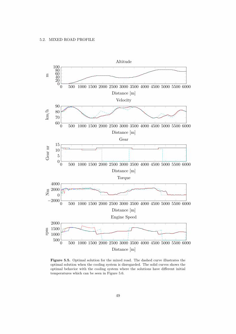
5.2. MIXED ROAD PROFILE
0 500 1000 1500 2000 2500 3000 3500 4000 4500 5000 5500 600060708090
Distance [m]
km/h
Velocity
0 500 1000 1500 2000 2500 3000 3500 4000 4500 5000 5500 6000020406080
100
Distance [m]
m
Altitude
0 500 1000 1500 2000 2500 3000 3500 4000 4500 5000 5500 600005
1015
Distance [m]
Gearnr
Gear
0 500 1000 1500 2000 2500 3000 3500 4000 4500 5000 5500 6000−2000
020004000
Distance [m]
Nm
Torque
0 500 1000 1500 2000 2500 3000 3500 4000 4500 5000 5500 6000500100015002000
Distance [m]
rpm
Engine Speed
Figure 5.5. Optimal solution for the mixed road. The dashed curve illustrates theoptimal solution when the cooling system is disregarded. The solid curves shows theoptimal behavior with the cooling system where the solutions have different initialtemperatures which can be seen in Figure 5.6.
49
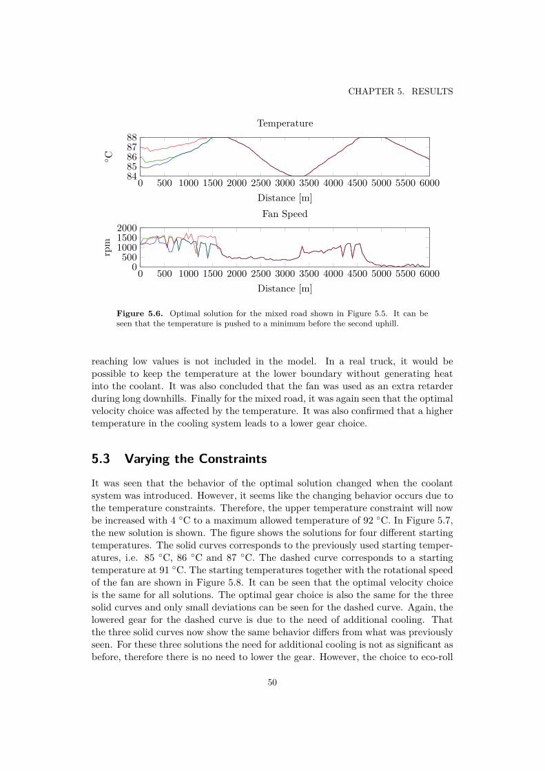
CHAPTER 5. RESULTS
0 500 1000 1500 2000 2500 3000 3500 4000 4500 5000 5500 60008485868788
Distance [m]
◦ CTemperature
0 500 1000 1500 2000 2500 3000 3500 4000 4500 5000 5500 60000500
100015002000
Distance [m]
rpm
Fan Speed
Figure 5.6. Optimal solution for the mixed road shown in Figure 5.5. It can beseen that the temperature is pushed to a minimum before the second uphill.
reaching low values is not included in the model. In a real truck, it would bepossible to keep the temperature at the lower boundary without generating heatinto the coolant. It was also concluded that the fan was used as an extra retarderduring long downhills. Finally for the mixed road, it was again seen that the optimalvelocity choice was affected by the temperature. It was also confirmed that a highertemperature in the cooling system leads to a lower gear choice.
5.3 Varying the Constraints
It was seen that the behavior of the optimal solution changed when the coolantsystem was introduced. However, it seems like the changing behavior occurs due tothe temperature constraints. Therefore, the upper temperature constraint will nowbe increased with 4 ◦C to a maximum allowed temperature of 92 ◦C. In Figure 5.7,the new solution is shown. The figure shows the solutions for four different startingtemperatures. The solid curves corresponds to the previously used starting temper-atures, i.e. 85 ◦C, 86 ◦C and 87 ◦C. The dashed curve corresponds to a startingtemperature at 91 ◦C. The starting temperatures together with the rotational speedof the fan are shown in Figure 5.8. It can be seen that the optimal velocity choiceis the same for all solutions. The optimal gear choice is also the same for the threesolid curves and only small deviations can be seen for the dashed curve. Again, thelowered gear for the dashed curve is due to the need of additional cooling. Thatthe three solid curves now show the same behavior differs from what was previouslyseen. For these three solutions the need for additional cooling is not as significant asbefore, therefore there is no need to lower the gear. However, the choice to eco-roll
50

5.3. VARYING THE CONSTRAINTS
0 500 1000 1500 2000 2500 3000 3500 4000 4500 5000 5500 600060708090
Distance [m]
km/h
Velocity
0 500 1000 1500 2000 2500 3000 3500 4000 4500 5000 5500 6000020406080
100
Distance [m]
Altitude
Altitude
0 500 1000 1500 2000 2500 3000 3500 4000 4500 5000 5500 600010111213
Distance [m]
Gearnr
Gear
0 500 1000 1500 2000 2500 3000 3500 4000 4500 5000 5500 6000−2000
020004000
Distance [m]
Nm
Torque
0 500 1000 1500 2000 2500 3000 3500 4000 4500 5000 5500 6000100012001400160018002000
Distance [m]
rpm
Engine Speed
Figure 5.7. Optimal solution with the new temperature constraints. The dashedcurve corresponds to the new starting temperature at 91 ◦C which can be seen inFigure 5.8.
51

CHAPTER 5. RESULTS
0 500 1000 1500 2000 2500 3000 3500 4000 4500 5000 5500 600086889092
Distance [m]
◦ CTemperature
0 500 1000 1500 2000 2500 3000 3500 4000 4500 5000 5500 60000500
10001500
Distance [m]
rpm
Fan Speed
Figure 5.8. Optimal solution for the mixed road shown in Figure 5.7. The maximumallowed temperature is now 92 ◦C.
is still not optimal for any of the solutions. It was previously suggested that eco-rollwas not chosen due to that the vehicle was unable to accelerate to the desired ve-locity where eco-roll became beneficial. In Figure 5.8, it is seen that the fan is usedwith low speed up for the first hill, which is the section between 0-1500 m. However,it would be possible to increase the rotational speed of the fan and thus increase thecooling. By doing this, the temperature would be lower and it would probably bepossible to accelerate the vehicle faster and thereafter go to eco-roll. It could be thecase that using the fan with higher rotational speed during the first uphill wouldincrease the fuel consumption more than what is earned from eco-rolling. Thus, itcould be that it is not only the constraints that affect the optimal solution, but alsothe loss of engine power and the increased fuel consumption which arise when thefan is used.
To conclude the results, it is clear that the cooling system affects the optimalsolution. The behavior is changed more close to the temperature constraints. Whenthe temperature is free to vary and when there is no need to use the fan, the optimalsolution seem to be the same. This will be discussed further in the next chapter.
52

Chapter 6
Conclusion
In this final chapter, the work conducted in this thesis will be concluded. First, themain parts of this thesis will be summarized in Section 6.1 which is followed by adiscussion in Section 6.2. Finally, potential future work is proposed in Section 6.3.
6.1 Summary
The work of the thesis started with an investigation of the auxiliary devices. Theinvestigation showed that the auxiliaries can consume a significant part of the totalengine power. The total average power consumption of the auxiliaries is just below10 kW which equals approximately 1 % of the maximum engine power. However,during uphill slopes, the consumption can reach values up to 10 %. It was shownthat the oil and coolant pumps are two of the largest consumers of energy, witha mean consumption of approximately 2 kW each. Further, it was also shownthat the two auxiliaries that consume the maximum amount of energy were the aircompressor and the cooling fan. However, the abilities to control these two lowertheir mean consumption.
It was further investigated how the consumption of the auxiliaries depended ondifferent factors, such as the road profiles. The investigation showed that the maincauses that influence the consumption of the auxiliaries were the temperature andthe inclination of the road. The cooling system was the system mostly affectedby the incline. It was concluded that heat flowed into the cooling system both indownhill and uphill slopes which lead to a higher demand of cooling, and thus ahigher fan usage. There was no ambient temperature dependence for the coolingsystem but the dependence was found for the air compressor and the AC compressor.The AC compressor was used more during warmer temperatures, while the aircompressor was used more during lower temperatures.
Different approaches for reducing the consumption of the auxiliaries were shownin Chapter 3. It is clear that the consumption of the auxiliaries can be reduced.Yet there are high demands on robustness and the potential energy saving must beevaluated compared to the effort of redesigning the auxiliaries. In this thesis, the
53

CHAPTER 6. CONCLUSION
approach to not change the hardware setup of the auxiliaries was taken. However,electrically controlled auxiliaries will most likely be used in the future and becauseof this, the efficiency of the generator should be improved.
An optimal control problem for the cooling system was formulated in Chapter 4.The control problem optimized gear and velocity choice together with the desired fanusage. The solution for the control problem with the cooling system was comparedto the control problem without the cooling system in Chapter 5. It was clearlyseen that the temperature in the cooling system affects the optimal velocity andoptimal gear choice, particularly around the temperature boundaries. However, thecomplexity of the solution makes the problem hard to solve in real time. Even ifthe solution is improved, it is probably not worth the effort to run the optimizationalgorithm with the cooling system included. However, it could be beneficial toestablish rules for example the gear choice when the temperature is high and aroundthe upper constraint. It should also be remembered that it was only the coolingsystem that was included in this thesis. It is very likely that other systems such asthe air system or the after treatment system also affects the optimal velocity andgear choice. Thus, it should be asked how optimal the original solution for gearsand velocity actually is.
6.2 Discussion
The impact of the auxiliaries on the total fuel consumption could be seen as asmall proportion. It is shown that the consumption of an auxiliary is of average1 kW, which is a small number compared with the total output of the engine atapproximately 540 kW for the most powerful trucks. However, if all auxiliaries areengaged simultaneously, the total consumption can reach levels as high as 50 kW,which then equals 10% of the total engine power. This amount can not be neglectedwith regard to fuel consumption or gear choice.
It is reasonable that a long-haulage truck is used at least 8 hours a day. If thefuel mass flow is calculated as above, a power consumption of 1 kW would yielda fuel mass flow of approximately 0.05 g/s which could seem like a small amount.The mass flow per hour is thus approximately 0.16 kg/h and with the density ofdiesel fuel at 0.832 kg/l it is quickly concluded that the consumed diesel in litersper hour equals approximately 0.2 l/h. Assuming that the total consumption of theauxiliaries equals 10 kW and with the truck up and running 8 hours per day, thetotal fuel consumption of the auxiliaries during one day would equal approximately15 liters per day. With the diesel price around 14 SEK/l, the cost for the auxiliariesequals 210 SEK per day. This means that the total cost for the energy of theauxiliaries for 300 days a year equals 63 000 SEK. Reducing the total consumption ofthe auxiliaries with 1 kW, would therefore give a saving of 7000 SEK per year. Thiscost should be used as a limit for how much the cost for the auxiliaries can increase.It would not be feasible to optimize the auxiliary devices for a large developmentcost which only leads to small savings for the costumer. Apart from this, it is
54

6.2. DISCUSSION
likely that the pressure from governmental environmental laws will increase, whichwould mean that the consumption has to be decreased regardless the cost of theimprovements. It must also be remembered that this is only the cost to power theauxiliaries.
It is well known that an increased engine temperature would lead to increasedefficiency for the combustion process. With the higher efficiency, the fuel savingswould likely increase. The optimal solution given in Chapter 5 would also most likelychange when the solution try to reach efficient combustion temperatures. The fanwould probably be engaged more and the temperature would probably fluctuateless. However, the new solutions depend on how much the temperature of theengine affects the efficiency of the combustion. As mentioned, a fuel rate dependingon the torque and engine speed was chosen. For more accuracy, a more detailedfuel map with the engine temperature included should probably be used. However,with regard to the implementations aspects, small differences of the solution shouldbe disregarded.
Other solutions for improvement were also discussed. For example, improvingthe efficiency of the alternator. If the efficiency of the alternator would be twice ashigh, half the power would be required to the alternator. This would lead to savingabout roughly 5000 SEK per year.
A conclusion regarding the energy savings of coordinating the cooling systemwith the control of velocity and gear choice is not ready to be drawn. It is shownboth in this and previous work that better control of different devices with use ofroad data would increase the performance and lower the fuel consumption. However,the downside of coordinating the control for different devices is that it gives riseto complex problems to solve. Even though the search space for the optimizationalgorithm is limited, it is doubtful that the algorithm can be executed in real time.The most likely approach for implementing a near to optimal solution is to use theinformation from the optimization problem and establish rules for the control of thedifferent devices. This approach is as mentioned taken in [10], but only the roadprofile is taken into account. As shown in this thesis, it could be optimal to decreasethe engine torque or lower the gear instead of using the fan. That is why rules forthe torque control in the engine could also be based on the engine temperature.However, the optimal solution is always of use since the control implementationscan aim to be similar to the optimal solution.
If rule based control for the cooling system and the engine with gearbox were tobe implemented, it would be a good choice to keep these control modules separated.This is because the optimal velocity and gear profiles are not influenced much duringnormal temperatures and normal fan usage. However, when the temperature in thecooling system reaches critical values where it is known that the optimal gear andvelocity profiles change, the cooling system module makes the engine control moduleaware of this. When the engine control module is aware of that the cooling systemis at critical levels, the engine control could apply strict measures, for examplelimiting the torque or limiting the gear choice. Another solution could be to usean optimization algorithm in real time for gears and velocity, where either the cost
55
CHAPTER 6. CONCLUSION
or the constraints change depending on the temperature in the cooling system. Asimple example could be to add a penalty for high gears when the temperature inthe cooling system is high. While the temperature is high, the optimal solutionwill be to use lower gears which leads to that the fan can be used with highervelocity to lower the temperature. When the temperature is back to normal valuesthe penalty is removed and optimization problem is changed back to the originalproblem. However, the optimal solution for the overall system needs to be knownbefore rules can be implemented.
6.3 Future WorkTo further continue to study the auxiliaries, they should be examined with morestatistical methods. It is important that the data provided is for a large amountof vehicles, even though it was shown that the behavior of the auxiliaries oftenare similar for the three vehicles examined in this thesis. Regarding redesign ofthe auxiliaries, much work could be done. It is likely that there will be higherdemands on controllability of the auxiliaries in the future. Therefore, a probablefuture scenario is electrified devices. However, the redesign of the auxiliaries willcome naturally with new engines powered with for example electricity.
For the optimal control problem, the first thing to continue with is to furtherlimit the search space or to solve the optimization problem differently. Without amore limited search space, the complexity of the optimization problem will becometo large when more auxiliary systems are introduced. As mentioned, the optimalsolution is of great value since rules can be established and implemented in the realsystem. This is probably the future approach to take, even though a centralizedoptimized system would probably be more efficient and appealing.
To end the thesis, it should be remembered that there are still improvements thatcan be made regarding the fuel consumption of the auxiliary devices. Controlledauxiliaries would likely improve the fuel consumption. Also, driving the vehicle withsmart adaptive cruise controllers could as well reduce the fuel consumption. How-ever, the auxiliary systems seem to change the optimal driving profile, which shouldbe taken into account when controllers are designed for optimal fuel consumption.
56
Bibliography
[1] Mustafa Abdul-Rasool. The impact of ecoroll on fuel consumption - using lookahead. Master’s thesis, KTH, Automatic Control, 2011.
[2] Christian Andersson. On Auxiliary Systems in Commercial Vehicles. PhDthesis, Lund, Department of Industrial Electrical Engineering and Automation,2004.
[3] Elias Bartos and Kristian Ahlberg. Minimizing of drain leakage on a scaniaretarder. Master’s thesis, KTH, Vehicle Dynamics, 2011.
[4] Richard Bellman. Dynamic Programming. Dover Publications, 1957.
[5] Dymola. http://www.dynasim.se/, June 2013.
[6] Erik Hellström. Look-ahead control of heavy trucks utilizing road topography.Technical report, 2007. LiU-TEK-LIC-2007:28, Thesis No. 1319.
[7] Åke Huttunen. Kombinerat hydrauliskt och el-mekaniskt styrservosystem.Master’s thesis, Linköpings Universitet, 2011.
[8] Maria Ivarsson. Fuel optimal powertrain control for heavy trucks utilizing lookahead. Technical report, 2009. LiU-TEK-LIC-2009:8, Thesis No. 1400.
[9] Uwe Kiencke and Lars Nielsen. Automotive Control Systems, For Engine,Driveline, and Vehicle. Springer Verlag, 2nd edition, 2005.
[10] Niclas Lerede. Topography based fan control for heavy trucks. Master’s thesis,Linköping University, SE-581 83 Linköping, 2009.
[11] Matlab/Simulink. http://www.mathworks.se/, June 2013.
[12] V.V. Monastyrsky and I.M. Golownykh. Rapid computation of optimal controlfor vehicles. Transportation Research Part B: Methodological, 27(3):219 – 227,1993.
[13] Gustav Norman and Mengxi Wu. Optimal driving strategies for minimizingfuel consumption and travelling time. Master’s thesis, KTH, Optimization andSystems Theory, 2013.
57

BIBLIOGRAPHY
[14] Niklas Pettersson. Modelling and Control of Auxiliary Loads in Heavy Vehicles.PhD thesis, KTH, Signals, Sensors and Systems, 2004.
[15] Carl-Johan Sjöstedt. Evaluation of auxiliary device efficiency in heavy vehi-cle application. In Proceedings of the ASME 2013 International Design Engi-neering Technical Conferences & Computers and Information in EngineeringConference, Portland, Oregon, USA, August 2013.
[16] Carl Wahlström. Modellering och utvärdering av en reglerbar termostat. Mas-ter’s thesis, Uppsala Universitet, 2012.
[17] Pelle Windestam. Simulation of power saving potential for auxiliary units inheavy commercial vehicles. Master’s thesis, KTH, Department of aeronauticaland Vehicle Engineering, 2008.
58