Simulation and Evaluation of Slurry Erosion

Erik Grimm Strømme

Master of Science in Mechanical Engineering

Supervisor: Reidar Kristoffersen, EPTCo-supervisor: Stein Tore Johansen, EPT

Jone Rivrud Rygg, Aker Solutions

Department of Energy and Process Engineering

Submission date: June 2015

Norwegian University of Science and Technology

I

Preface This Master’s thesis was written at the Department of Energy and Process Engineering at the

Norwegian University of Science and Technology during the spring of 2015.

The object of this thesis was developed in cooperation with the Subsea department at Aker

Solutions.

First, I want to thank my academic supervisor, Reidar Kristoffersen for guidance and support

during this semester. Also, big thank you to my two industrial advisors at Aker Solutions, Jone

Rivrud Rygg and Guruprasad Kulkarni for your help, advice and important discussions during

our weekly telephone-meetings. A thank you must also be given to Robert Johansson for

providing me useful IT equipment and licenses, and to make this cooperation possible in the

first place.

My sincere thank you goes to my fellow students at the Waterpower Laboratory for all the good

discussions and the great work environment.

Last but not least, a special thank you to Benedicte, for motivating me every day along the way,

also outside the grey walls. Your support has been invaluable.

Have fun!

_______________________________

Erik Grimm Strømme

Trondheim, June 2015

II

Abstract Erosion from sand particles is a large problem in piping systems, especially in the oil and gas

industries. Different types of erosion occur depending on the concentration of particles present

in the fluid. Computational Fluid Dynamics (CFD) is a promising tool for erosion prediction,

with different models available for erosion calculations. The most commonly studied erosion

models are the Lagrangian impact based. These are simplified models, and they put a limit to

model flows where particle concentrations increases.

The aim for this Master’s thesis has been to investigate and assess available models in ANSYS

Fluent for evaluating slurry erosion rates.

First, a literature study was carried out in order to understand how slurry flows behave under

different flow conditions, how erosion from different sand particle concentrations are modeled

and which models that are available ANSYS Fluent for these calculations. An important part

of the study was to find available experimental results regarding erosion rates in literature,

which could be replicated into CFD as validation of the erosion models.

The Lagrangian Discrete Phase Model (DPM) approach was used to validate the DNV erosion

model against an experimental case with low particle concentration. A Slurry flow case

simulation with the Eulerian model with a Dense Discrete Phase Model (DDPM) was set up on

the same case in order to see if the model could capture the abrasive wear from the particles.

All results from the DPM and DDPM simulations were written to file, plotted and compared

with experimental results. Attempts were made in order to include the Discrete Element Method

(DEM) collision model into the erosion simulations.

It was found that the DNV impact based erosion model shows good agreement with the

experimental result by capturing the location and magnitudes of erosion rate. When including

the Eulerian DDPM on the same geometry, results did not change much on the low particle

concentration case. Thus, abrasive wear became more dominant as the particle concentration

increased which is because of the increase of the wall shear stress from the slurry flow.

Since no suitable cases were found in literature regarding slurry erosion rates, an experimental

case with higher particle concentrations should be performed so the models for slurry erosion

can be validated.

III

Sammendrag Erosjon fra sandpartikler er et stort problem når det kommer til rørsystemer, spesielt ved

produksjon av olje og gass. Ulike typer av erosjon kan forkommer avhengig av konsentrasjonen

partikler som er til stede i fluidet. Computational Fluid Dynamikk (CFD) er et nyttig verktøy

for å beregne erosjon, med ulike erosjon modeller tilgjengelig for å utføre beregninger. Den

mest brukte erosjonsmodellen er en Lagrange modell som baserer seg på enkelt partikler som

treffer en overflate. Dette er forenklede modeller og egner seg ikke til modellering av løsninger

med høyere partikkel konsentrasjoner.

Målet med denne masteroppgaven har vært å undersøke og vurdere tilgjengelige modeller i

ANSYS Fluent for å evaluere erosjonsrater fra slurrier.

Først ble et litteraturstudie gjennomført for å forstå hvordan slurry-strømning oppfører seg

under forskjellige strømningsforhold, hvordan erosjon fra ulike sandkonsentrasjoner kan

modelleres og hvilke modeller som er tilgjengelig i ANSYS Fluent for denne type beregninger.

En viktig del av studiet var å finne tilgjengelige eksperimentelle resultater vedrørende

erosjonsrater, kopiere forsøket inn i CFD og bruke den for validering av erosjons-modellene.

For å validere DNVs erosjonsmodell mot eksperiment ble det benyttet en Lagrange Discrete

Phase Model (DPM) tilnærming da partikkelkonsentrasjonen var lav. Det ble også gjort

simuleringer på samme geometri for et tilfellet med høyere konsentrasjon av partikler. Her ble

en Eulerian modell benyttet med en inkludert Dense Discrete Phase Model (DDPM) for å

undersøke om modellen plukket opp slitasje fra partiklene som skled langs veggen. Resultatene

fra DPM og DDPM ble skrevet til fil, plottet og sammenlignet med eksperiment-resultatene.

Det ble i tillegg gjort forsøk på å inkludere kollisjonsmodellen Discrete Element Method

(DEM) i simuleringene.

Erosjonsmodellen til DNV viste seg å gi gode resultater sammenlignet med eksperimentet, og

fanget opp erosionsratens størrelsesorden samt lokasjon. Simuleringer med Eulerian DDPM på

den samme geometrien endret ikke resultatene stort for tilfellet med lav partikkelkonsentrasjon.

Slitasjen fra partiklene derimot ble mer synlig og dominerende ettersom partikkel-

konsentrasjonen økte, som var forventet på grunn av økningen av skjærspenningene på veggen

fra slurrien. Siden ingen egnede eksperiment ble funnet i litteraturen for å validere slurry

erosjonsmodellen, bør det utføres et eksperiment med høyere partikkelkonsentrasjoner.

IV

Contents

Preface ......................................................................................................................................... I

Abstract ..................................................................................................................................... II

Sammendrag ............................................................................................................................. III

List of Figures .......................................................................................................................... VI

List of Tables ........................................................................................................................... VII

Nomenclature ........................................................................................................................ VIII

1. Introduction ........................................................................................................................ 1

2. Theory ................................................................................................................................ 3

2.1 Slurry flow ................................................................................................................... 3

2.1.1 Physical properties and classification of a slurry ................................................. 3

2.1.2 Describing Slurry flows ....................................................................................... 5

2.1.3 Pressure gradient in slurry flows .......................................................................... 6

2.2 Erosion ......................................................................................................................... 9

2.2.1 Particle impact erosion ....................................................................................... 11

2.2.2 Slurry erosion ..................................................................................................... 13

2.2.3 Experimental methodologies for predicting erosion .......................................... 14

2.3 Theoretical Background of Computational Fluid Dynamics ..................................... 18

2.3.1 General ............................................................................................................... 18

2.3.2 Governing Equations .......................................................................................... 18

2.3.3 Equation of Motion for Particles ........................................................................ 19

2.3.4 Turbulent modeling ............................................................................................ 21

2.4.3.1 The law of the wall and y+................................................................................ 22

2.4.3.2 k-ϵ turbulence model ........................................................................................ 24

2.4.3.3 k-ω and Shear Stress Transport model ........................................................ 25

2.4.3.4 Wall Interactions .............................................................................................. 26

2.3.5 Multiphase flow modeling ................................................................................. 27

2.3.5.1 Lagrangian Discrete Phase Model .............................................................. 28

2.3.5.2 Discrete Element Method ........................................................................... 29

2.3.5.3 Euler-Euler Approach ................................................................................. 31

2.3.6 Verification and validation ................................................................................. 34

3. CFD Analysis in ANSYS Fluent ...................................................................................... 35

3.1 Validation of the DNV erosion model ....................................................................... 36

V

3.1.1 Geometry and meshing ....................................................................................... 36

3.1.2 Pre-process ......................................................................................................... 37

3.1.3 Particle tracking and Post processing ................................................................. 39

3.2 Eulerian Model with DDPM ...................................................................................... 39

3.2.1 Geometry and meshing ....................................................................................... 40

3.2.2 Pre-process ......................................................................................................... 41

3.2.3 Post processing for Eulerian modeling ............................................................... 43

3.3 Simulations with DEM collision model .................................................................... 44

4. Results and Discussion ..................................................................................................... 45

4.1 Validation of the DNV impact erosion model ........................................................... 45

4.2 Eulerian model with DDPM ...................................................................................... 50

4.2.1 Straight pipe results ............................................................................................ 51

4.2.2 Eulerian simulations on DNV’s Bean Choke ..................................................... 52

4.3 DEM collision model ................................................................................................. 55

5. Conclusion ........................................................................................................................ 56

6. Recommendations for Further Work ................................................................................ 58

7. References ........................................................................................................................ 59

Appendices ............................................................................................................................... 61

Appendix A .......................................................................................................................... 61

Appendix B .......................................................................................................................... 62

Appendix C .......................................................................................................................... 67

Appendix D .......................................................................................................................... 72

VI

List of Figures

Figure 2.1: Four flow regimes for a settling, heterogeneous slurry in horizontal pipelines

(King, 2002, p. 84). .................................................................................................................... 6

Figure 2.2: Schematic representation of the flow regimes for settling slurries in horizontal

pipelines (King, 2002, p. 84). ..................................................................................................... 6

Figure 2.3: Momentum transfer between the fluid and the wall during slurry flows through a

pipe (King, 2002, p. 82). ............................................................................................................ 7

Figure 2.4: Pressure drop – velocity relation of heterogeneous slurry flow through a pipe

(Mali et. al, 2014, p. 2). .............................................................................................................. 8

Figure 2.5: Impact angle definition (Huser & Kvernvold, 1998, p.4). ..................................... 12

Figure 2.6: Function F(α) for typical ‘ductile’ and brittle materials (DNV, 2007) .................. 12

Figure 2.7: Bean Choke geometry (Huser & Kvernvold, 1998, p. 5). ..................................... 15

Figure 2.8: Slurry loop design with all equipment (Loewen, 2013, p.53). .............................. 16

Figure 2.9: Boundary layers near wall ..................................................................................... 22

Figure 2.10: The law of the wall. ............................................................................................. 24

Figure 2.11: «Reflect» boundary condition for the discrete phase (ANSYS Fluent, 2013,

24.4.1) ....................................................................................................................................... 27

Figure 2.12: Heat- mass- and momentum transfer between the discrete and continuous phases

.................................................................................................................................................. 28

Figure 2.13: Particles represented as spheres (ANSYS Fluent, 16.12.1). ................................ 30

Figure 3.1: ANSA-mesh with thin inflation layers .................................................................. 37

Figure 3.2: Hex-mesh used for the straight pipe simulation. ................................................... 40

Figure 4.2: Fluid solution over the contraction. ....................................................................... 46

Figure 4.1: Contour of y+ values in the cell layer closest to the wall. ...................................... 46

Figure 4.3: Contour of the erosion rate after the contraction, with maximum erosion. ........... 47

Figure 4.4: Contour of erosion rate on the 45° wall. ................................................................ 47

Figure 4.5: Result of the DPM simulation. .............................................................................. 48

Figure 4.6: Particle distribution along the straight pipe. .......................................................... 51

Figure 4.7: Contour of erosion rate along the pipe. ................................................................. 52

Figure 4.8: Plot of the results with different particle loading with DDPM and the DPM. ...... 53

VII

List of Tables

Table 2.1: Sand particle definition (ISO 14688-1, 2002). .......................................................... 4

Table 2.2: Different types of wear from sand particles. ........................................................... 10

Table 2.3: Parameters affecting erosion (Eltvik, 2013, p. 9). .................................................. 10

Table 2.4: Material constants for steel (DNV, 2007, p. 11) ..................................................... 11

Table 2.5: Constants to be used in equation 2.6 (DNV, 2007, p.10). ...................................... 12

Table 2.6: Important independent variables present that influence slurry erosion (Wood et. al,

2001, p. 774). ............................................................................................................................ 13

Table 3.1: Overview of simulations ......................................................................................... 35

Table 3.2: Mesh-info for the chosen grids. .............................................................................. 37

Table 3.3: Fluid Parameters ..................................................................................................... 38

Table 3.4: Particle parameters .................................................................................................. 39

Table 3.5 Mesh info ................................................................................................................. 40

Table 3.6: Important parameters used for the Eulerian DDPM simulation with DNV. ........... 42

Table 3.7: Additional parameters used for the abrasive wear simulation. ............................... 42

Table 4.1: Overview of simulations ......................................................................................... 45

VIII

Nomenclature

Cv solid concentration by volume αsp packing volume fraction Cw solid concentration by mass τ linearization coefficient ρm mixture density CD drag force coefficient ρs solid density Re Reynolds number ρl liquid density τij stress tensor

ΔP pressure drop y+ dimensionless distance

fsl friction factor u+ near wall velocity E erosion Rate Ut

tangential velocity

Pm particle mass flow rate τω wall shear stress

K material constant uτ skin friction velocity n material constant κ von Karman constant

VnP particle impact velocity B log layer constant

At target area exposed to erosion ke turbulent kinetic energy ρt target density ω turbulent frequency

Cunit conversion factor μt turbulent viscosity F(α) ductility of target material

α impact angle Abbreviations Ai constants ANSYS Analysis Systems Sij rate of stress tensor CFD Computational Fluid Dynamics δij kronecker delta-tensor DDPM Dense Discrete Phase Model Fall sum of forces acting on particles DEM Dense Element Method ø generic transported value DNV Det Norske Veritas

FD drag force DPM Discrete Phase Model up particle velocity RANS Reynolds Averaging Navier-Stokes u fluid velocity SIMPLE Semi-Implicit Method for Pressure

Linked Equations ηs Coulumbic friction αs particle volume fraction SST Shear Stress transport

1

1. Introduction Erosive wear of both production and injection pipes is a big problem in the petroleum industry,

where the consequences can be crucial. A mixture of water, oil, gas and sand particles are

transported through miles of pipeline, and due to variation of velocities and the fluid properties,

material loss in different equipment is considered a risk. It is therefore desirable to be able to

accurately predict the rate of erosion.

The most commonly studied erosion mechanism is particle impact based erosion, calculating

material removal based on particle impact velocity and angle. Particle impact based erosion is

a risk mainly in gas and water flows where particles are suspended in the fluid. Another erosion

mechanism often seen in the oil and gas industry is the slurry erosion. This happens due to the

wall shear stress of the slurry along the pipe. These slurries are fluids with a large amount of

solids, and this type of erosion can be seen even at low fluid velocities as the particles are sliding

along a surface. Operations such as for instance drilling, cementing involve the use of slurries

transported through the system.

Computational Fluid Dynamics (CFD) is a useful tool for predicting erosion. Even though the

CFD modeling of erosion have been done for years, there is still a need of deeper knowledge

about the models and methods available in the programs. Particle impact based erosion models

available in CFD are only valid for specific low particle loading cases since the model neglects

the occupied volume by the particles. This is an Eulerian-Lagrangian modeling of dispersed

particles, and puts a limit to model flows as particle loadings increase. At higher particle

loading, which is arguably the general case for slurry transport, particle to particle interaction

comes into play. In general, slurry erosion is much more complex than particle impact erosion,

making it difficult to predict. The simulation of these flows should be treated as fully coupled

with an Eulerian-Eulerian approach. A method for prediction of slurry erosion is the topic of

this thesis, where both Lagrangian and Eulerian models available in CFD should be tested for

flow with higher particle loading.

In this thesis, an attempt has been made to develop a method using ANSYS Fluent as CFD

software to model erosion from a slurry flow with a particle concentration higher than accepted

for the Lagrangian impact based models. The DNV, Lagrangian approached impact based

erosion model was first validated against experimental erosion results on a Bean Choke,

reported by Huser & Kvernvold (1998). With this model validated, an Eulerian model with the

2

Dense Discrete Phase Model (DDPM) as an Eulerian parameter was set up and simulated in

Fluent.

An experimental test case with higher particle concentration, reported by Loewen (2013), was

supposed to be used as validation case for the Eulerian DDPM model. It appeared that the wall

material used in the test-section was a polymer and not a metal. This became a problem in the

simulations since the available models in Fluent require material constants, which are only

available for some metals. Because of this, the experimental results were not suitable for the

erosion model validation. Instead, the experimental results regarding the flow field and particle

distribution were used to set up the Eulerian DDPM simulations. Simulations with this setup

were then performed on the same Bean Choke geometry from Huser & Kvernvold (1998) in

order to see the effect on erosion when the particle concentration was increased.

By using the different, available, erosion models, and the combination of the validated particle

impact wear model and the abrasive wear model from ANSYS, erosion rate results from a slurry

flow were captured and reported. This thesis report should give a good explanation of how these

results are obtained, through both relevant theory and the presentation of how the simulations

have been performed.

3

2. Theory This chapter is covering the relevant theory, and is divided into three sections. The first section

describes the slurry flow and its physical properties. The second presents the most common

erosion processes present in a pipeflow of a continuous phase and a solid phase. Both particle

impact and sliding abrasion are described. In the third section, the theory behind the CFD

simulations are described, and how ANSYS Fluent is solving the governing equations for these

simulations.

2.1 Slurry flow Slurries are a solid-liquid mixture with a large amount of solids. A slurry can sometimes be

classified as a high viscous fluid. Since the particle concentration is high, it is important to

understand the physical principles for this type of flow and also to classify the slurries. With

the high particle concentration, the erosion phenomena will occur. Slurry erosion is an erosion

mechanism that occur due to the wall shear of the slurry flow through a pipe combined with

random particle impacts.

2.1.1 Physical properties and classification of a slurry It is important to classify a slurry in order to provide a basis for describing the physical

appearance and the flow behavior of the two-phase solid-liquid mixture, i.e. rheology. Rheology

is the study of the flow of matter, and applies to substances with complex structures such as

slurries. The rheology is a dynamic property of the microstructure of the slurry and is affected

by various attributes such as the shape, density, size and mass fraction of the suspended solid

particles and the density and viscosity of the carrier fluid (Roitto, 2014, p. 6).

The classification of the slurry flow is also important when it comes to designing pipelines. The

most commonly used attributes used to characterize a slurry are the basic physical properties of

the constituents, in particular those of the solids (Brown & Heywood, 1991, p. 3):

x Density of the constituent phase,

x Concentration of solids,

x Characteristic particle size or more appropriately, particle size distribution and

x Characteristic particle shape.

Depending on the particle size, it is usual to classify the particles as coarse, medium and fine

particles depending on their diameter. ISO 14688-1 (2002) lists the basic principles for the

4

classification of different soils most commonly used for engineering purpose, and the size-range

for sand is shown in Table 2.1 (ISO 14688-1, 2002):

Size range, d [mm] Description

0.063 ≤ d ≤ 0.2 Fine

0.200 ≤ d ≤ 0.63 Medium

0.630 ≤ d ≤ 2.0 Coarse Table 2.1: Sand particle definition (ISO 14688-1, 2002).

The Density of the slurry is affected by the density of the carrier fluid, the density of the solid

particles and the concentration of solid particles present. The solid concentration can be

expressed by volume or weight fraction. The relationship between these two can be expressed

as (Wasp, 1977, p. 46):

(2.1)

where

Cv = concentration by volume in percent

Cw = concentration of solids by weight in percent

ρm = density of mixture [kg/m3]

ρs = density of solid [kg/m3]

ρl = density of liquid [kg/m3]

And from this relation, the density of slurry is defined as (Wasp, 1977, p. 45):

(2.2)

Depending on the particle concentration, slurries can be classified as a dilute or a dense slurry.

A dilute slurry flows have a low particle volume concentration (<5-10%), where erosion occur

mainly due to particle impact on the walls. For the dense slurries flows, the particle volume

concentration is higher and the particle-particle interaction becomes more important than for

dilute slurries (Brown & Heywood, 1991, pp. 7-8).

100

100

w

w m sV

w ws

s l

CCC C C

U UU

U U

�

�

100100m

w w

s l

C CU

U U

�

�

5

2.1.2 Describing Slurry flows To understand the erosion phenomena in a solid-liquid pipe flow, it is important to look at the

flow regimes in the dense slurry transport. Information of velocity and particle concentrations

profiles will give an indication of the solids distribution in the pipe cross-section.

Depending on the particle size and velocity, slurries are usually associated with settling

tendencies. If the velocity though a pipe is low and the particle size is large, particles will tend

to sink and settle at the bottom pipe wall. This is called a Newtonian, settling slurry. If the

particle size is smaller, the slurry can be classified as a non-settling slurry and may exhibit a

non-Newtonian behaviour. Particles then remain in suspension for a long time. For a slurry flow

through a pipe, velocity must then increase as particle size increases in order to avoid the slurry

to settle and keep particles suspended (Brown & Heywood, 1991, pp. 41-42). If particles settle

at lower speed, they can block the pipe as a worst case scenario.

Since non-Newtonian flow is very complex and a complete study itself, the viscous effects are

neglected in this thesis. That means that the slurry flows are at any time defined as a both

settling and Newtonian, and the viscosity of the fluid remains constant and is independent of

any external stresses, and the shear rate that is affects it. An example can be the forces acting

on the fluid from the particles.

By the settling tendency under the influence of gravity, transport of slurry flow can be classified

into four different flow regimes in a horizontal pipe. Concentration is usually higher in the

bottom layer of the cross-section, and the extent of the solid concentration is dependent on the

velocity and the turbulence. With high velocity and high turbulence levels, the suspension is

almost homogeneous with very good dispersion of the solids. With low turbulence levels, the

particles will settle towards the wall and be transported as a sliding bed under the influence of

the pressure gradient in the fluid. If the turbulence levels are not high enough to maintain a

homogeneous suspense but still sufficiently high to prevent any deposition of particles on the

wall in the pipe, the flow regime is described as a heterogeneous suspension. As the velocity of

the slurry reduces further, a distinct mode of transport known as saltation regime develops. In

this regime, there is a visible layer of particles in the bottom wall in the pipe, and they are being

6

continuously picked up by turbulent eddies along the pipe (King, 2002, pp. 83-84). The four

flow regimes for settling slurries in horizontal pipes are shown in Figure 2.1.

The relationship between frictional pressure gradient and the slurry velocity varies from regime

to regime and they can be approximately delimited in the particle size vs. slurry velocity as

shown in Figure 2.2 (King, 2002, p. 84).

2.1.3 Pressure gradient in slurry flows With flow taking form of the four different regimes from a sliding bed of mud to a homogenous

suspension, a number of different factors will interact in a horizontal pipe. With transportation

of a settling, heterogeneous slurry, the influence of gravity will develop significant gradients in

the solid concentration. The solids will generate additional momentum transfer and need to be

Figure 2.2: Schematic representation of the flow regimes for settling slurries in horizontal pipelines (King, 2002, p. 84).

Figure 2.1: Four flow regimes for a settling, heterogeneous slurry in horizontal pipelines (King, 2002, p. 84).

7

considered when developing models for momentum transfer between the slurry and the pipe

wall. Particles moving faster than the fluid will transfer some of its momentum to the fluid, and

faster moving fluid will transfer momentum to the particles. This interaction with solid particles

and liquid in a two-phase flow, will also affect the momentum transfer from the two-phase to

the wall. Particles will dissipate some of their kinetic energy by hitting the wall. This will

increase the shear stresses from the fluid-particle and the wall, i.e. higher friction drag force

through the pipe (King, 2002, pp. 81-82). The additional path through which momentum can

be transferred from the fluid to the solid wall during a settling slurry through a pipe can be

illustrated as done in Figure 2.3 (King, 2002, p. 82).

This additional momentum transfer through the pipe will affect the pressure drop because of

friction from the particles. Compared to the pressure drop through the pipe with only a single

fluid present, the solid particles momentum transfer will increase the pressure drop. This is

expressed in equation 2.3 (King, 2002, p. 82).

(2.3)

Where ΔPf,sl is the pressure drop due to friction from the slurry transport, ΔPfw is the pressure

gradient if only the fluid were present flowing at the same velocity as the slurry. This pressure

gradient can also be calculated from the relationship between the wall shear stress and pressure

gradient, and vice versa (King, 2002, p. 82).

(2.4)

where ρw is the density of water and not the slurry density.

,f sl fw additionalP P P' ' �'

2

, 2f sl sl wLP f VD

U'

Figure 2.3: Momentum transfer between the fluid and the wall during slurry flows through a pipe (King, 2002, p. 82).

8

By calculating the pressure drop, and then the friction factor, it is possible to use the Moody

diagram to find the friction coefficient ε in the pipe with particles in the domain.

A typical pressure drop – velocity relation of a heterogeneous slurry flow through a pipe is

given in Figure 2.4. The pressure drop with only water present in the pipe is also shown as a

comparison (Mali et. al, 2014, p. 2).

At higher velocities (point 4) the curve tend to be parallel to the simple fluid response through

the pipe. At higher velocities than 4, slurry flow becomes homogenous and the concentration

gradient becomes less dominant. As the velocity decreases, the solids are still suspended, but

the distribution becomes heterogeneous. When the velocity reach point 3, the solids start to

form a sliding bed i.e. saltation regime. At this point, the slurry reach the critical velocity, where

the pressure drop is at its minimum. With an even further speed reduction of the flow (point 2),

more of the solids are transported as a bed load through the pipe. This tendency of particles

settling as a stationary bed increases until point 1, where the solids stop moving (Mali et. al,

2014, pp. 1-2).

The critical velocity (point 3) is the most useful since at this point the head loss is at its

minimum, and is defined as when particles are no longer transported through the pipe in

suspension or whether or not the bed is moving or stationary (Wasp, 1977).

Figure 2.4: Pressure drop – velocity relation of heterogeneous slurry flow through a pipe (Mali et. al, 2014, p. 2).

9

2.2 Erosion Erosive wear, commonly known as erosion is defined as material loss resulting from impact of

solid particles on the material surface (DNV, 2007, p. 10). In complex piping systems, with

sand particles present in the fluid, particles sliding, rolling, colliding or hitting the material

surface will result in material deformation, cutting, fatigue cracking or a combination of these.

With different influencing factors on erosion from sand particles, different types of wear

mechanisms can occur. Before going deeper into the types of wear relevant for this thesis, a list

of some relevant wear mechanisms from particle impacts are listed in Table 2.2 (Meng &

Lundema, 1995, pp. 449-450):

Mechanism of erosion Definition Illustration

Abrasive erosion Particles strike the wall at

low impact angles and

material is removed by

cutting. The particles act

like a bed that is sliding

over the surface.

Fatigue wear Particles strike the surface

at low speed, but a with a

large impact angle. The

surface material cannot be

plastically deformed, but it

becomes weak due to

fatigue action. After

repeated hits, cracks will

occur in the material and

particles will be detached

from the surface after

multiple hits

10

Brittle fracture Erosion by brittle fracture

when particles hit the wall

with medium velocity and

high impact angle. This is

likely to happen when the

particles have sharp edges.

Saltation wear Transport of a sediment

where particles are moved

forward along the pipe in

series, bouncing along the

wall.

Table 2.2: Different types of wear from sand particles.

From the different definitions above, it is clear that the extent of the removed material is

dependent on various parameters such as particle and material properties, flow conditions and

the particle volume fraction present in the fluid flow. These are listed in Table 2.3 (Eltvik, 2013,

p. 9):

Flow conditions Relative velocities between interacting

surfaces- Impact velocity, impact angle,

particle mass flow rate, turbulence-,

centrifugal-, cavitation forces, viscosity

Particle properties Particle size, density, shape and concentration

Material properties Material hardness, ductility, coating, strength

Table 2.3: Parameters affecting erosion (Eltvik, 2013, p. 9).

During transport of slurries through a pipe at a typical bulk velocity, the particles settle at the

lower pipe wall due to gravitational forces. This creates a dense, sliding bed of particles that

moves slower than the fluid along the pipe. This action of the solid bed inflicts the erosive

damage on the pipe walls. This is the wear mechanism better known as abrasive wear and is

one of the main wear mechanisms in slurry erosion. The remaining particles above the bed is

assumed to be suspended by turbulence effects and particle lift forces. These effects cause

particles to impinge against the pipe walls, and this erosion effect is called impact based

erosion. These are the two dominant erosion models in slurry transport, and are described in

the following chapters.

11

2.2.1 Particle impact erosion Solid particle erosion is the loss of material that results from repeated impact on a surface of

small, solid particles. This type of erosion can be expected in any gas or liquid flow with hard

particles present. The particles are affected by the fluid which carries them along the flow

(Kosel, 1992, p. 199).

The first models developed for predicting erosion are based on the movement of a single

particle. Since then, different models have been developed in order to calculate erosion from

solid particles, and what they have in common are that they all requires a lot of input about the

flow conditions and the particles parameters. If these parameters are known, the erosion rate, �̇�

can be calculated from the general relation in the Recommended Practice written by Det Norske

Veritas, DNV (DNV, 2007, p. 14):

(2.5)

where

�̇�𝑃, is the particles mass flow rate.

K and n, is the material constants, which are determined by experimental investigations given

in Table 2.4 (DNV, 2007, p. 11).

Material K [(m/s)-n] n [-] Ρ [kg/m3]

Steel 2.0 × 10-9 2.6 7800

Table 2.4: Material constants for steel (DNV, 2007, p. 11)

𝑉𝑃𝑛 , is the impact velocity of particle and n is a material constant.

𝐴𝑡, is the area exposed to erosion, target area.

𝜌𝑡, is the targets density.

𝐶𝑢𝑛𝑖𝑡 , is a conversion factor from [m/s] to [mm/year].

The function 𝐹(𝛼) characterises the ductility of the target material, given by the relation;

(2.6)

� �˙

3

V 1 0 , 3.15 10

nP P m

unit unitt t t t

m K F E mmE C C EyrA AD

U U� � ª º

� « »¬ ¼� �

� � � �� �1 1 180

ii

iF A D SD � �§ · � ¨ ¸© ¹

¦

12

where the 𝐴𝑖’s are given in Table 2.5 (DNV, 2007, p. 10):

In equation 2.6, α is the impact angle, which is defined as the angle between the particle and

the wall. Figure 2.5 show the impact angle with a particle approaching the wall with a velocity,

u (Huser & Kvernvold, 1998, p.4):

Ductile materials attain maximum erosion attacks for impact angles in the range of 15°-30°

while brittle materials at a normal impact angle. For this thesis, the steel grades are regarded as

ductile material. The relationship between function F(α) an the impact angle is shown in Figure

2.6 (DNV, 2007, p. 12).

𝐴1 𝐴2 𝐴3 𝐴4 𝐴5 𝐴6 𝐴7 𝐴8

9.370 42.295 110.864 175.804 170.137 98.398 31.211 4.170 Table 2.5: Constants to be used in equation 2.6 (DNV, 2007, p.10).

Figure 2.5: Impact angle definition (Huser & Kvernvold, 1998, p.4).

Figure 2.6: Function F(α) for typical ‘ductile’ and brittle materials (DNV, 2007)

13

In the DNV erosion model, the blue curve for ductile material is used as the boundary condition

on the wall for the particle impact function. More details on this is described later in this thesis.

2.2.2 Slurry erosion Slurry erosion is defined as the type of wear that occur when a material is exposed to a slurry

flow of higher particle loading. Shook & Roco (1991) have defined the erosion in dense slurry

flow as having three components including direct impact of particles; random impingement of

particles in turbulent motion and the friction of a sliding bed of particles pressing onto the wall,

known as abrasive wear.

The slurry erosion phenomena is complex due to the number of important independent variables

present that influence these three components. In Table 2.6, some of the main variables are

listed (Wood et. al, 2001, p. 774):

Slurry variables

Liquid Viscosity, density, surface activity, lubricity, corrosivity,

temperature

Particles Brittleness, size, density, relative velocity, shape, relative

hardness, concentration, particle-particle interactions

Flow field Angle of impingement, particle impact efficiency, boundary

layer, wall shear stress, particle rebound, degradation, particle

drop-out, turbulence intensity

Component variables

Bulk properties Ductility or brittleness, hardness, melting point, microstructure,

shape and roughness

Surface properties Work hardening, corrosion layers, surface treatments, coating

type, coating bond, microstructure

Service variables

Contacting materials, pressure, velocity, temperature, surface

finish, lubrication, corrosion, hydraulic design, intermittent

slurry flows. Table 2.6: Important independent variables present that influence slurry erosion (Wood et. al, 2001, p.

774).

14

In a slurry pipeline, the hydraulic gradients, i.e. head losses, are a key parameter. In literature,

the main component of head loss that is documented, which is contributing to wear from a

slurry, is the velocity independent Coulombic friction. The Coulombic friction is the relation

between particle stresses in different direction. For example by saying that τyy is fixed by

gravity, and if motion occurs in x-direction the stresses are related by a coefficient of Coulombic

friction, ηs (Gillies, 1993, p. 15):

(2.7)

This coefficient depends on the nature of the two surfaces and is caused by sliding motions of

the particles along the pipe wall. Lubrication effects reduce the coefficient of friction for

particles, which is moving parallel to the wall, if a liquid layer is separating them. Therefore,

this friction coefficient can be neglected further away from the wall, since the particles is fully

suspended in this area.

Based on results published in literature, the Coulombic friction is high at low velocities where

particles experience minimal lifting force. At higher velocities, the Coulombic friction

diminishes as the particle-bed cross-section diminishes (Loewen, 2013, p. 20). The minimum

friction occur at the critical velocity as presented in chapter 2.1.3.

Slurry erosion is dependent on various parameters as mentioned above, but more important is

how the flow-field looks like and how high the particle loading is. As described in chapter 2.1.2,

the classification of the slurry is dependent on the concentration of the solid and fluid properties.

The amount of abrasive wear is dependent on the particle concentration and again by the bulk

velocity through the pipe. By increasing the velocity, avoiding particles to settle, the erosion

damage due to particle impact will increase as the flow is more heterogeneous and particles are

suspended in the fluid. This will also reduce the abrasive wear along.

2.2.3 Experimental methodologies for predicting erosion Erosion studies have been performed for many years, and many different methods have been

used to get experimental results when it comes to wear of materials from sand particles.

Experiments have focused on sand concentration profiles, velocity profiles and frictional

pressure gradients. These results have been important in order to understand the flow field with

different particle loading. When it comes to experimental results regarding erosion rate, or just

material removal, not much have been reported. One of the benefits with a laboratory test is

that it is possible to have control over a wide range of parameters, for example sand

yx s yyW K W

15

concentration, which is a varying factor in the actual cases in nature. These are complex

experiments, and as discussed earlier; many factors and parameters must be taken into account

to keep control of the experiment.

In this thesis’s literature study, a lot of time have been spent in order to find reliable experiments

to replicate and model into CFD, and to compare the numerical results with the experiment. It

should be possible to see how good the CFD predicts erosion, both the impact based and the

slurry erosion. The focus have been to find data from tests performed in pipes so it is easier to

relate the results to the actual case for oil-production. In general, the pipe loop tests are small

scale versions of the real pipes. In order to have fully control of the flow, there is a flow

controller in the loop. The loop usually includes more than one test section with different

geometries; straight pipe, t-bends and 90° bends are some examples. In this chapter, the

experiments that are used and replicated in this thesis are presented briefly.

An experiment reported by DNV is used as a test for the Lagrangian erosion models (Huser &

Kvernvold, 1998, pp. 5-6). Carbon-dioxide gas at subsonic speed is sent through a Bean Choke

as shown in Figure 2.7. The gas enters a large diameter pipe, goes through a contraction and

exits through a smaller diameter outlet-pipe. It is clear that the velocity will increase as the area

after the contraction is lower, and it is expected that the fluid especially in this area will affect

particles. The following flow and particle parameters are applied to the experiment (Huser &

Kvernvold, 1998, pp. 5-6):

- Inlet velocity: 11,4 [m/s]

- Inlet pressure: 14.1 [bar]

- Inlet temperature: 36 oC

- Fluid Viscosity: 1.5x10-5 [kg/(ms)]

- Inlet diameter: 54 mm

- Outlet diameter: 20 mm

- Particle diameter: 0.25 mm

The above experiment from DNV is suitable for testing impact based erosion models in CFD

since the particle concentration is low. For denser slurries, there are limited with performed

experiments available in literature regarding erosive wear and slurry erosion. The only reported

case found in the literature study in this thesis is from the University of Alberta, US, where a

large test-rig has been built and the master thesis student, Derek John Loewen, has reported his

Figure 2.7: Bean Choke geometry (Huser & Kvernvold, 1998, p. 5).

16

experimental work regarding Characterization of Wear in a Laboratory-Scale Slurry Pipeline

(2013). The experiment examines few selected parameters during the tests in order to

understand the principal parameters and therefor these assumptions are made (Loewen, 2013,

p. 51);

- Two-phase water-sand slurries are used in order to eliminate non-Newtonian effects,

bitumen-related wall roughness and air bubbles affecting the flow.

- This allows focus to remain on mechanical wear, without being concerned with the

compounding effects of corrosive and erosive-corrosive wear.

- Mass flow rate and bulk solids concentration is controlled within the process. Particle

size and the sensitivity of the size is not included in the study, and an average size is

kept constant.

The setup of the slurry loop design with all equipment is shown in Figure 2.8 (Loewen, 2013,

p. 53).

The testing section is a removable tube-section that consists of a two slip-on steel flanges

supported by four threaded rods. The test pieces may be fitted into the flanges and tightened in

Figure 2.8: Slurry loop design with all equipment (Loewen, 2013, p.53).

17

place with nuts. The test material for the pipe-wall was first chosen to be PVC, but even after

65 hours of being subjected to slurry flow at high pump speed; the PVC did not show any visible

scratches or signs of wear. Therefore, urethane was used as coating on the inner walls, with 2.7

mm thick layer (Loewen, 2013, pp. 64-65). Urethane is a polymer which have lower density

than steel, and erosion from sand particles is easier to get visible.

The following flow and particle parameters were applied to the experiment:

- Outer pipe diameter: 57.15 mm

- Wall thickness: 2.7 mm

- Length of test section: 488.15 mm

- Particle concentrations: 6.4 and 13.5 [vol%]

- Average particle diameter: 1.5 mm

- Mass flow rate: ~5, ~6 and ~9 [kg/s]

Erosion rate results in [kg/hr/m] are given for different pump speeds i.e. mass flowrates.

18

2.3 Theoretical Background of Computational Fluid Dynamics When modeling turbulent flow in pipes with sand present, the treatment near the wall is

important to do correctly. This is because the turbulence can have a significant influence on

erosion my particle impact. In Computational Fluid Dynamics (CFD), numerical methods and

physical models are available for predicting the approximate mean motion and trajectories of

particles suspended in turbulent flows (Dosanjh & Humphrey, 1985). This chapter provides a

brief description of the CFD and the applications used in this thesis.

2.3.1 General CFD is a set of numerical methods applied to obtain approximate solutions of problems of fluid

dynamics and heat transfer (Zikanov, 2010, p. 1).

The equations governing the fluid flow have been known for a century. The equations are

complex, but their solutions are very useful to understand fluid flows, regarding both the

dynamics and heat transfer. Unfortunately, these equations cannot be solved in general. A

numerical approach is used as a computational procedure to find an approximation to the

solution. This approach outperforms the theoretical and the experimental approach in some very

important aspects; universality, flexibility, accuracy and cost (Zikanov, 2010, pp. 2-3).

2.3.2 Governing Equations Three governing equations describes the conservation laws of classic physics, namely:

x Conservation of mass

x Momentum equation

x Conservation of energy

In the process for the numerical approach solution, the fluid is regarded as a continuum; the

substance fills the given space it occupies. The computational domain is divided into a certain

number of small elements, where the elements are large enough compared with the sizes of the

molecules to treat the fluid as a continuum. These elements are called fluid elements (Zikanov,

2010, pp. 11-12).

When the fluid moves through these elements, conservation laws must be satisfied and the

equations can be presented on differential form;

The continuity equation requires conservation of mass:

19

(2.8)

The Navier-Stokes equation is derived from the Newton’s 2nd law:

(2.9)

where Sij is the rate of strain tensor and δij is the Kronecker delta-tensor

The energy equation is only necessary if the flow is compressible or with thermal conduction,

which is not the case in this study.

ANSYS Fluent are using the finite volume technique by discretizing and solving the given

equations above in each of the fluid elements. This is a control-volume-based technique consists

of integrating the transport equation about each control volume. Starting with a transport

equation on the integral form (ANSYS Fluent, 2013, 20.2.):

(2.10)

The volume integrals is then discretized within the element and accumulated to the control

volume to which the sector belongs. Surface integrals are discretized at the integration points

located at the center of the each surface segment within the element and then distributed to the

adjacent control volumes:

(2.11)

with subscript f as a value within the control volume (ANSYS Fluent, 2013, 20.2.).

With just a few adjustments, equation (2.10) can be used for each of the control volumes in the

given domain. This will result in a set of algebraic equations that can be solved using iterative

methods, such as conjugate gradient, multigrid etc.

2.3.3 Equation of Motion for Particles ANSYS Fluent calculates the trajectory of a discrete phase particle by integrating the force

balance on the particle, which is done in a Lagrangian approach. This force balance equates the

particle inertia with forces acting on the particles such as drag, pressure, buoyancy and added

mas or virtual forces. This can be written as (ANSYS Fluent, 16.2.1.1.):

� � 0 ii

ut xU Uw w�

w w

� � � � 2 (2 )3

ki i j ij ij i

j j j k

upu u u S ft x x x xU U P P G Uww w w w

� � � � �w w w w w

� � øV V

dV v d A d dVA St I

UIUI I

w� � * � � �

w³ ³ ³ ³

� � � � faces facesN N

ff ff

S f ff

vV A A S Vt I I

UIU II

w� � * � � �

w ¦ ¦

20

(2.12)

where,

is the fluid phase velocity,

is the particle velocity,

is the fluid density,

is the density of the particle.

is the drag force per unit particle mass and

(2.13)

where,

is the molecular viscosity of the fluid,

Re is the relative Reynolds number, which is defined as

(2.14)

and the drag coefficient for spherical particles is taken from Morsi and Alexander (1972)

experiments, with constants a1, a2 and a3 that apply over several ranges of Re (Morsi &

Alecander, 1972, p. 195) :

(2.15)

in equation (2.12) is an additional acceleration term. This includes additional forces that can

be special under different circumstances, and is defined under the physical setup for particles.

For this thesis, the following additional forces are important (ANSYS Fluent, 2013, 16.2.1.3.):

1. Virtual mass force is required to accelerate the fluid surrounding the particle. This term

can be written as:

(2.16)

where Cvm is the virtual mass factor with default value of 0.5.

( )( )p p

pDp

gdu F u u Fdt

U UU�

� � �

u

pu

U

pU

( )D pF u u�

2

Re1824D

Dp p

CFdP

U

P

Rep pd u uU

P

�{

321 2Re ReD

aaC a � �

F

( )ppvm

p

duF C u udt

UU

� �

21

2. Pressure gradient force comes as an additional force which is arising from the pressure

gradient in the fluid:

(2.17)

The two forces are important when the density ratio between particle and fluid is greater than

0.1. This means that for a sand-gas flow, where ρ/ρp << 1, it is not important (ANSYS Fluent,

2013, 16.2.1.3.).

2.3.4 Turbulent modeling The flow becomes turbulent above a critical Reynolds number (White, 1999, pp. 325-330).

Today, the most common approach in industry to solve the turbulence is by using the Reynold

Averaging Navier-Stokes (RANS) model. For the RANS model, the pressure and velocity is

decomposed into mean and fluctuating components:

(2.18)

(2.19)

Introducing these expressions into the N-S equation (2.9) and averaging:

' ' 2(u )ii j i

j i

u pu g ut x x

U U U Pw w w� � � �

w w w (2.20)

also continuity;

Rewriting the equation to include the stress tensor, from the relation:

Equation (2.20) becomes:

iij

i

u pgt x

U U Ww w � ���

w w (2.21)

p

p

F u uUU

�

Re 2300 , Re = critUDUP

|

' i i iu u u �

p p pc �

0i

i

uxw

w

� � iij i j

j

u u ux

W P Uw �

wc c

22

Performing the time-averaging operation on the momentum equations, all the details of the state

of the fluid contained in the rapid fluctuations is gone. The result yields six additional unknown

functions, which is the Reynold stresses. The main task of turbulence modeling is to develop

computational procedures of sufficient accuracy and generality for engineers to predict the

Reynolds stresses and the scalar transport terms (Versteeg & Malalasekera, 1996, 5, pp. 75-78).

Before introducing the turbulence models, the modeling near the wall will be described.

2.4.3.1 The law of the wall and y+ Close to a wall, with the no-slip condition, a boundary layer will rise as shown in Figure 2.9.

The velocity goes from zero at the wall to the free stream velocity further away from the wall.

In a turbulent flow, the variations will be largest in the near wall region, and this will cause the

strongest gradients to occur here. Solving the governing equations near the wall is therefore

difficult due to the variations of the dependent variables, such as velocity and the wall shear

stress. Since in this project it is important to capture the near wall gradients, a large number of

nodes are needed.

The boundary layer near the wall consists of two layers:

1. Viscous sublayer, y+ < 5. A thin layer

next to the wall where viscosity has a

greater influence since the flow on

average behaves close to laminar.

In the viscous sublayer;

y+ = u+

2. Logarithmic layer is the region between the viscous sublayer and the fully turbulent layer.

Here where the mixing turbulence is the dominant variable, with 60<y+<200. In this layer, u+

is proportional with ln (y+). This relation is called the law of the wall, see equation (2.22).

In between these two layers, 5<y+<60, there is a region called the buffer layer. Here, the flow

is still dominant of viscous effects, but turbulence are becoming significant.

In ANSYS Fluent there are two approaches to model the near-wall region;

1. One approach is using semi-empirical formulas called wall functions to bridge the region

between the wall and the fully-turbulent region. This means that the region covering the viscos

Figure 2.9: Boundary layers near wall

23

region and the buffer layer is not resolved. The advantage using this method is that a coarse

mesh can be used to model high gradient shear layers near the wall, and this will save

computational cost by saving CPU time and storage.

2. In the other approach, the turbulence models are modified to resolve the viscosity-affected

region close to the wall. This requires a fine mesh into the viscous sublayer (ANSYS Fluent,

2013, 4.14.1.1.). This second method is known as the low Reynolds number method.

Turbulence models based on the ω-equation are suitable for low Reynolds, like the SST as will

be explain later. This method requires higher computational power than the wall function, since

more storage and runtime is required.

The standard wall functions in Fluent is an extension of the Launder-Spalding method, which

involves the following steps (Bredberg, 2000, pp. 11-12):

1. Solve the momentum equation with a modified wall viscosity.

2. Solve the turbulent kinetic energy, with modified integrated production and

dissipation terms.

3. Set epsilon using the predicted k.

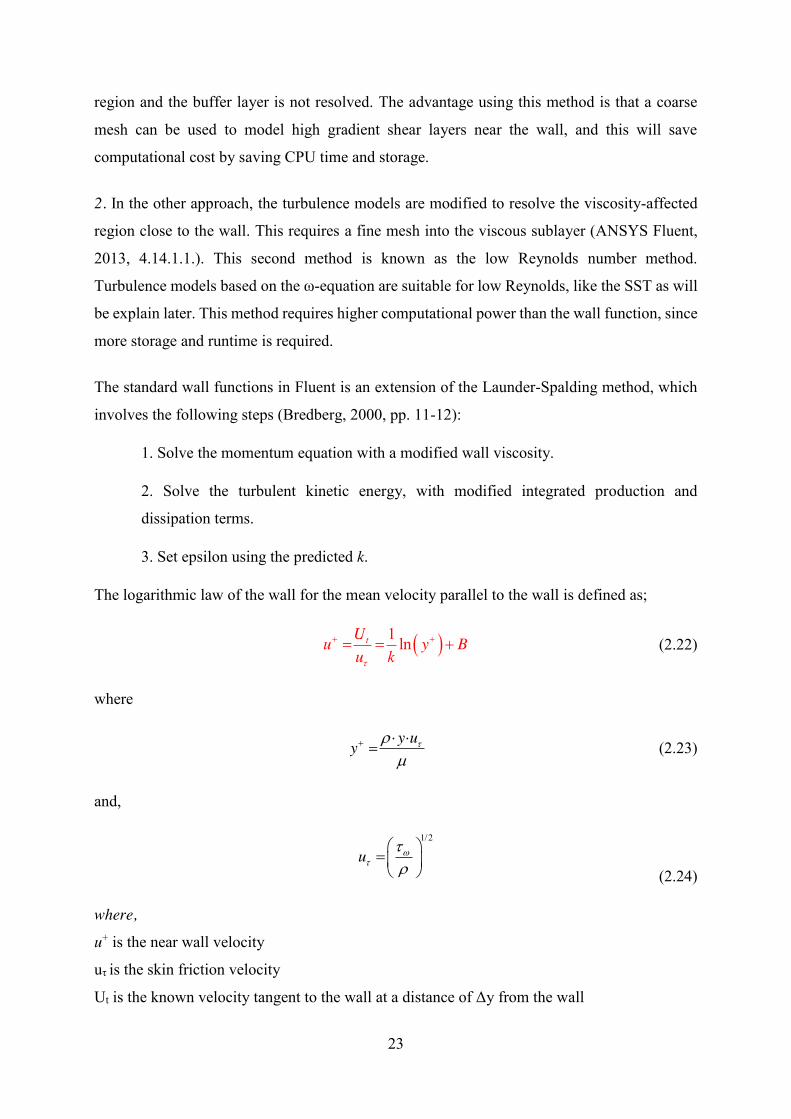
The logarithmic law of the wall for the mean velocity parallel to the wall is defined as;

(2.22)

where

(2.23)

and,

(2.24)

where,

u+ is the near wall velocity

uτ is the skin friction velocity

Ut is the known velocity tangent to the wall at a distance of Δy from the wall

� �1 lntUu y Bu kW

� � �

y uy WUP

� � �

1/2

u ZW

WU

§ · ¨ ¸© ¹

24

y+ is the dimensionless distance from the wall

τω is the wall shear stress

κ is the von Karman constant

B is the log layer constant depending on the wall roughness.

In Figure 2.10, the law of the wall and the logarithmic-law is compared.

Equation (2.22) has a downside becoming singular at separation points where the near wall

velocity approaches zero, therefore a scalable wall-function is needed. This function uses an

alternative velocity scale, u* instead of uτ. The standard wall function gets weak when the mesh

is refined, and then the scalable function can be applied on arbitrarily fine mesh and allows

performing a consistent mesh refinement independent of the Reynolds number (ANSYS Fluent,

2013, 4.14.3.).

The dimensionless distance from the wall, y+ is important in CFD because it is important to

know the location of the first node away from the wall.

2.4.3.2 k-ϵ turbulence model This is a two-equation model within the RANS models, which means that two transport

equation needs to be solved, one for the turbulent kinetic energy, k, and one for the turbulent

dissipation, ϵ, which is the rate of dissipation of k.

The k-ϵ model is well tested and the most widely used turbulence model. It is known to be

successful solving a wide variety of industrial relevant flows without changing the model

constants. It is particularly well in confined flows where the Reynolds shear stresses are most

Figure 2.10: The law of the wall.

25

important.

Limitations for the model are weak shear layers, Boundary layer separation, flows over curved

surfaces and rotating flows (Versteeg & Malalasekera, 1995, pp. 74-75).

In Fluent the k-ϵ uses the scalable wall-function approach to improve robustness and accuracy

when the mesh close to the wall is fine, but it will not resolve the boundary conditions. By using

the k-ϵ in near wall modelling, the flow is assumed to have the characteristics as a fully

developed turbulent boundary layer. Instead of solving the governing equation in the first cell

closest to the wall, the velocity profile is assumed to be as in the law of the wall, Figure 2.10.

The usage of this scalable wall-function requires the first node from the wall to be in between

30 < y+ < 300. The model is not suitable for flows with separation and flow over curved

surfaces.

The turbulent viscosity, , is computed by combining k and ε as follows (ANSYS Fluent,

2013, 4.3.1.2.):

(2.25)

where is a constant.

2.4.3.3 k-ω and Shear Stress Transport model

When the k-ϵ model fail and the ϵ- models fail to solve the separation, other models are needed

to model the flow. The most prominent two-equation model in this area is the k-ω model.

Compared to the k-ϵ, this model does not involve the complex damping functions if it gets

integrated down to the viscous sublayer. By solving the low Reynolds number method, this

model is a preferred choice when it comes to near wall treatment. A low-Reynolds number k-

ω requires at least y+< 5. The model assumes that turbulence viscosity, μt, is linked to turbulent

kinetic energy ke, and turbulent frequency, ω, via the relation (ANSYS Fluent, 2013, 4.4.1.3.):

(2.26)

With the coefficient, , as a damping of the turbulence viscosity causing a low-Reynolds

number correction.

tP

2

= Ctk

PP UH

CP

*= tkUP DZ

*D

26

The k-ω model is used in another model called the Shear Stress Transport (SST) model. It

accounts for, as from the name, the transport of turbulent shear stress. It is designed to give a

more accurate prediction of the onset and the amount of flow separation under adverse pressure

gradients.

The SST model in Fluent is using an automatic near-wall treatment by applying both the wall-

function and the low-Reynolds number approach. This is done by using the k-ϵ for the free-

stream and the k-ω for at the viscous sublayer. The model is similar to the k-ω but includes the

following refinements (ANSYS Fluent, 4.4.2.1.):

x The standard k-ω model and a transformed k-ϵ model are both multiplied by a blending

function and added together. The blending function is in the near-wall region which

activates the k-ω model.

x The definition of the turbulent viscosity is modified to account for the transport of the

turbulent shear stress.

The SST model will therefore require a y+≤ 5 and at least 10 inflation layers near the wall as

for the k-ω model. Between the extremes, the SST uses a blending function to achieve a mix of

the k-ϵ and k-ω. SST model should give the best results when the flows are separated, and

should be a preferred choice of model flow including particles.

2.4.3.4 Wall Interactions With different particle impacts on the wall along a pipe, it is important do go into how a CFD

code is treating this. Particles are transferring kinetic energy to the wall when hitting it. The

velocity after the particle-wall collision is dependent on the particle properties, the wall material

and the fluid phase. In Fluent, the restitution coefficient is providing this information when the

boundary condition for the wall is set to reflect the particles. This factor or coefficient defines

the amount of momentum, in the direction normal to the wall, which is retained after the

collision with the wall (ANSYS Fluent, 2013, 24.4.1.):

(2.27) 2,

1,

nn

n

ve

v

27

Figure 2.11 show the “reflect” boundary condition for the discrete phase:

This means that a restitution effect of 1.0 implies that the particle retains all its kinetic energy

after the rebound, and the collision is elastic. If it is less than 1.0, the collision is inelastic and

the kinetic energy of the particle is less than before the impact.

Particles may also in some cases stick to the wall or remain very close to the wall after hitting

it. For these situations, special boundary condition need to be developed. A tangential or normal

coefficient of restitution equal to 0.0 implies that the particle stick to the wall.

2.3.5 Multiphase flow modeling Multiphase flow is defined as a fluid flow consisting of more than one face or component. In

this thesis, where sand particles are transported with the fluid through a pipe, the simulation

have to be handled as a multiphase flow simulation.

Multiphase flow can be classified into three different groups:

1. Dispersed flows: Particles, bubbles or droplets in the liquid.

2. Intermittent flow: Slug and annular flow as a gas-liquid mixture.

3. Separated flow: liquid and gases.

Currently, there are two different types of approaches for numerical calculation of multiphase

flow. They will be described in the following chapters and are based on these descriptions;

Lagrangian description will track the position and velocity of a small number of particles

through the continuum fluid. The motion of an individual particle is based on the Newton’s

laws. The advantage using the Lagrangian method is that it is very useful describing particles

behavior.

Figure 2.11: «Reflect» boundary condition for the discrete phase (ANSYS Fluent, 2013, 24.4.1)

28

Eulerian description will define a control volume or a flow domain. It is possible to describe

the flow properties at every point in space as time varies. This way of looking at the motion of

the fluid is by focusing on the specific location in the domain where the fluid flows as time

passes.

2.3.5.1 Lagrangian Discrete Phase Model The Lagrangian Discrete Phase Model (DPM) in ANSYS Fluent follows the Euler-Lagrange

approach. As a rule of thumb, particle concentration should be less than 10 vol% for this

approach for the model to work. The fluid is treated as a continuum by solving the time-

averaged Navier-Stokes equations. When the fluid is solved correctly, a large number of

particles are tracked through the field. When doing this, the particles are transported through

the fluid without affecting the fluid and without taking up any volume since this is neglected.

Therefore, also particle-particle interactions can be neglected (ANSYS Fluent, 2013, 16.1.1.).

With this fixed continuous phase, it is said to be a one-way coupling between the phases. It is

though possible to incorporate the effect of the discrete phase on the continuum and achieve a

two-way coupling between the phases. This is accomplished by alternately solve the discrete

and continuous phase equations until the solutions in both phases have stopped changing

(ANSYS Fluent, 2013, 16.13.1.). Illustration in Figure 2.12:

In Fluent, the particle trajectories are computed individually at specified intervals during the

fluid phase calculations. This is done by integrating the force balance on the particle as

described in chapter 2.3.3, which is written in a Lagrangian reference frame.

Figure 2.12: Heat- mass- and momentum transfer between the discrete and continuous phases

29

When simulating particle trajectories, the specified boundary condition needs to be set. The

most important boundary conditions are the one for the walls, which should represent a collision

between the particle and the wall. In this thesis, the erosion model used for the Lagrangian

approach, and later within the Eulerian model, is the DNV erosion model. This model is not

available in ANSYS Fluent, and has to be implemented manually. Particle erosion and accretion

rates can be monitored at wall boundaries and is calculated from the relationship shown in

chapter 2.2.1 in equation 2.5. The varying factor is the angle where the particles strike the wall.

This impact angle function has to be defined in the wall boundary under the Discrete Phase

Model (DPM) tab. For the DNV model, this impact angle function is the blue line in Figure 2.6

in chapter 2.2.1, since ductile materials are used in this thesis. This function is implemented by

using 15 points along the line, and it is added as a pricewise-linear fit.

It is also important to define both the diameter function, K and the velocity exponent function,

n in the equation, which is the material constants. The recommended values for steel are given

in Table 2.4 in chapter 2.2.1.

2.3.5.2 Discrete Element Method A model that need to be described is the Discrete Element Method (DEM) which is based on

the work of Cundall & Strack (1979), and accounts for the forces that result from collision

between particles. The method is based on the use of explicit numerical scheme in which the

interactions of the particles is monitored contact by contact and the motion of the particles are

modelled particle by particle (Cundall & Strack, 1979). The discrete element method is suitable

for simulations of granular flows, which are characterized by higher particle loading. DEM is

usually included in simulations where particle-particle interactions are important.

The force resulting from the particle collision will come as an additional force to the equation

1.12 in chapter 2.4.3. This is determined by the deformation, which is measured as the overlap

between pairs of spheres (ANSYS Fluent, 2013, 16.12.1.).

30

When two particles interact and bounces off each other, it can be looked at like in Figure 2.13

(ANSYS Fluent, 2013, 16.12.1).

The method is based on the spring constant, k, and the size of it when particles come in contact.

The value of k can be estimated from the following equation (ANSYS Fluent, 2013, 16.12.1.):

(2.28)

where,

D is the parcel diameter, ρ is the particle mass density, v is the relative velocity between

colliding particles, and εD is fraction of the diameter for allowable overlap.

The collision force laws used in this thesis for the DEM are:

1. The Spring-dashpot collision law is a linear spring force law with a dashpot and is used for

the normal forces.

2. The Friction Collision law is based on the equation for Coulomb friction (2.7) in chapter

2.2.2. This law is used for the tangential forces.

As for the DPM, the particles in DEM are not tracked individually but as parcels of particles.

Each parcel is the determined by tracing a single representative particle. The parcel approach is

2

23 D

vk DS UH

Figure 2.13: Particles represented as spheres (ANSYS Fluent, 16.12.1).

31

used in Fluent instead of single particle tracking because the computational cost is much lower.

DEM differs from DPM in following ways (ANSYS Fluent, 2013, 16.12.1.4):

- The mass used for DEM calculations of the collision is the one from the entire parcel

and not just the single particle.

- The radius of the DEM parcel is a sphere and the volume is the mass of the entire parcel

divided by the density of the particle.

When including the DEM collision model, the particle tracking changes to an implicit scheme,

which means an implicit Euler integration of equation (2.12) which is unconditionally stable

for all particle relaxation times (ANSYS Fluent, 2013, 24.2.7.1.).

2.3.5.3 Euler-Euler Approach This approach make it possible to treat each of the different phases mathematically as

interpenetrating continua. With a liquid- and solid phase present, the solids will occupy a

volume, which it is not in the Lagrangian approach. This introduce the phasic volume fraction.

These volume fractions are assumed to be continuous functions of space and time and their sum

is equal to one. Conservation equations for each phase are derived to obtain a set of equations,

which have similar structure for all phases. By providing constitutive relations that are obtained

from empirical information, the equations are closed. In case of a granular flow, these are closed

by application of kinetic theory (ANSYS Fluent, 2013, 17.2.1.1).

The simulations are said to be fully coupled, since the different phases interact with each other,

particle-particle interaction occur and the particles take up volume in the flow. This particle to

particle interaction will then come into play in both typical elastic particle-particle interaction

as well as grinding viscous interaction between particles. These interactions, and the turbulence

affecting the near-wall velocity, permits the particle to strike the wall at random impacts and

particle impact erosion occurs. Different patterns of solids in the flow can be observed

depending on the nature of the slurry and the flow conditions.

For denser slurries, with high particle concentration, a CFD simulation using this approach

should give the best results and give most reliable results. Within the Euler-Euler approach,

there are three different models available in Fluent. The Volume of fluid (VOF) model, the

Mixture Model and the Eulerian Model.

32

In this thesis, the model described and chosen is the Eulerian multiphase model. This model

also includes the Eulerian parameter, the Dense Discrete Phase Model (DDPM).

Eulerian Model with Dense Discrete Phase Model

The Eulerian model make it possible to model multiple separate, but with interacting phases.

Simulations with almost any type of combinations of solid-, liquid- and gas-phases can be

performed where an Eulerian approach is used for each phase. With this possibility of modeling

different phases, the only limitation is the memory requirements and convergence behavior.

This model is the most complex of the multiphase models, and therefore it is difficult to get a

converged solution (ANSYS Fluent, 2013, 17.15.1.).

The Eulerian model in Fluent is based on the following (ANSYS Fluent, 2013, 17.15.1.)

- A single pressure is shared by all phases

- Momentum and continuity equations are solved for each phase

- For a granular phase:

o Granular temperature can be calculated for each solid phase

o Solid-phase shear and bulk viscosities are obtained by applying kinetic theory

to granular flows.

- Several interphase drag coefficient functions are available for different types of

multiphase regimes.

- All the k-ε and k-ω turbulence models are available and can be applied to all phases of

mixtures.

The limitations of the Eulerian Model relevant for this thesis are the following (ANSYS Fluent,

2013, 17.5.2.):

- The Lagrangian particle tracking which is possible to combine with the model interacts

only with the primary phase. This DPM cannot be used with the model if the shared

memory option is enabled.

- The Reynold Stress turbulence model is not available per phase basis.

The Eulerian Model is using a concept of phasic volume fractions to describe the different

present phases. Volume fractions represents the space occupied by each of the phases, and the

laws of conservation of mass and momentum are satisfied by each phase individually (ANSYS

Fluent, 2013, 17.5.3.).

33

In this thesis, focusing on erosion and flow with particles, the Dense Discrete Phase Model

(DDPM) is included as an Eulerian parameter in the Eulerian Model. The DPM model as

described in chapter 2.3.5.1 includes the assumption that the volume fraction of the particles

are sufficiently low and are therefore neglected. In order to overcome this limitation of the

Lagrangian multiphase model, the volume fraction of the particle phase is accounted for in the

DDPM by extending the mass and momentum equations to the following equations. (ANSYS

Fluent, 17.5.18.).

This means that the DPM model is included within the DDPM while the particles takes up a

volume in the fluid. This model is capturing the abrasive wear from the particles sliding along

the wall by use of the wall shear stress and the solid phase velocity close to the wall. Particle-

particle interactions and volume fraction of solids are captured, and also the impacts of particles

also is included with the Lagrangian particle tracking.

The solid stresses acting on particles in a dense flow is modelled in Fluent by an additional

acceleration, , in the particle force balance from chapter 2.3.3. This addition is resulting

from inter-particle interaction (ANSYS Fluent, 2013, 17.5.18.2.):

(2.29)

The additional term is computed from the stress tensor given by the kinetic theory of granular

flows as:

(2.30)

interactionF

int( )

( )p peractionD p

p

du gF u u F F

dtU UU�

� � � �

int1

eraction sP

F WU

� �

34

2.3.6 Verification and validation In CFD modeling, it is essential to be aware of the quality and uncertainties the results contain,

and therefore be critical for them to be used. Verification and validation are two processes for

assessing the credibility of the CFD results.

Verification is defined as (Slater, 2008):

The process of determining a model implementation accurately represents the

developer’s conceptual description of the model and the solution to the model.

Verification assessment gives an indication if the computational models are the correct

implementation of the conceptual models. It will also examine if the code can be used for further

analysis based on the accuracy of the result. The different ways of doing this is to verify the

code, the iterative convergence, the consistency, the grid convergence and temporal

convergence (Slater, 2008).

Validation is defined as:

The process of determining the degree to which a model is an accurate representation

of the real world.

This includes comparing the CFD results with experimental data or to the results from a Direct

Numerical Solution if possible. In that case, it will only be possible to validate the code within

the range where there is experimental date available.

35

3. CFD Analysis in ANSYS Fluent The simulations in this thesis are rather complex and requires both a lot of memory and time to

perform. Because of this complexity, a lot of different simulations, with different mesh and

setups, have been performed to get best possible results. The simulation strategy and the

different procedures have been performed as presented in Table 3.1.

In order to present the results in an organized and clear way, this chapter is describing the setup

for the different simulations from the table in three different sections:

3.1: Validation of the DNV impact based erosion model against the Bean Choke

experiment using the DPM in Fluent, (Number 1). This chapter provides information

about the setup for the simulation, implementation of the DNV erosion model and post-

processing.

3.2: Simulation with the Eulerian model with DDPM is set up with the straight pipe case

from University of Alberta as a basis, (Number 2). With reliable results regarding the

flow-field in the straight pipe, the same setup is used on the Bean Choke case in order

to include the abrasive wear (Number 3). Several simulations are performed on the Bean

Choke with different particle concentrations and erosion rate calculations are explained.

3.3: The DEM collision model are included in simulation (Number 1) and (Number 3)

in order to see the effect of the collision model on both a Lagrangian and Eulerian

approach. Same procedure as the simulations, but with the DEM collision model

activated, (Number 4).

Number Multiphase Approach Multiphase Parameter Erosion Model Geometry

1 Lagrangian DPM DNV Bean Choke

2 Eulerian DDPM DNV+Abrasive Straight-pipe

3 Eulerian DDPM DNV+Abrasive Bean Choke

4 Lagrangian + Eulerian DEM DNV+Abrasive Bean Choke

Table 3.1: Overview of simulations

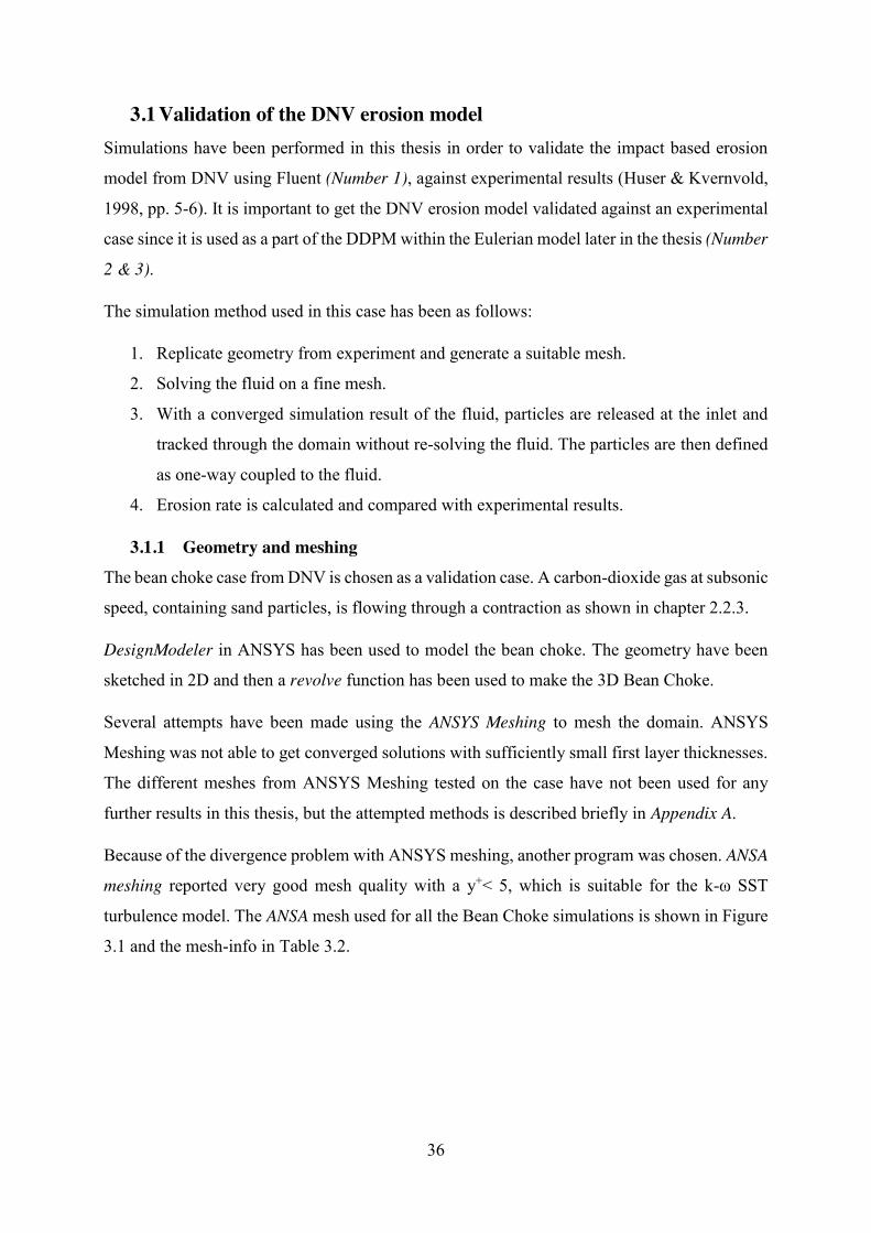
36

3.1 Validation of the DNV erosion model Simulations have been performed in this thesis in order to validate the impact based erosion

model from DNV using Fluent (Number 1), against experimental results (Huser & Kvernvold,

1998, pp. 5-6). It is important to get the DNV erosion model validated against an experimental

case since it is used as a part of the DDPM within the Eulerian model later in the thesis (Number

2 & 3).

The simulation method used in this case has been as follows:

1. Replicate geometry from experiment and generate a suitable mesh.

2. Solving the fluid on a fine mesh.

3. With a converged simulation result of the fluid, particles are released at the inlet and

tracked through the domain without re-solving the fluid. The particles are then defined

as one-way coupled to the fluid.

4. Erosion rate is calculated and compared with experimental results.

3.1.1 Geometry and meshing The bean choke case from DNV is chosen as a validation case. A carbon-dioxide gas at subsonic

speed, containing sand particles, is flowing through a contraction as shown in chapter 2.2.3.

DesignModeler in ANSYS has been used to model the bean choke. The geometry have been

sketched in 2D and then a revolve function has been used to make the 3D Bean Choke.

Several attempts have been made using the ANSYS Meshing to mesh the domain. ANSYS

Meshing was not able to get converged solutions with sufficiently small first layer thicknesses.

The different meshes from ANSYS Meshing tested on the case have not been used for any

further results in this thesis, but the attempted methods is described briefly in Appendix A.

Because of the divergence problem with ANSYS meshing, another program was chosen. ANSA

meshing reported very good mesh quality with a y+< 5, which is suitable for the k-ω SST

turbulence model. The ANSA mesh used for all the Bean Choke simulations is shown in Figure

3.1 and the mesh-info in Table 3.2.

37

ANSA-mesh

Nr. of elements 1293012

Nr. of nodes 1012186

Element size [mm] 1.0

First layer thickness [mm] 0.0001

y+ 3.5565

Table 3.2: Mesh-info for the chosen grids.

Several simulations with different meshes have been performed on the Bean Choke in order to

develop the final mesh. The main focus have been on the y+ value since this is important for the

fluid simulation.

3.1.2 Pre-process The simulation has been set up in ANSYS Fluent as a steady state simulation with a SIMPLE

Solution Method. The flow and particle parameters from the validation case by DNV are given

in Table 3.3 – 3.4. More details about the setup, see Appendix B for the Fluent input summary.

Figure 3.1: ANSA-mesh with thin inflation layers

38

In order to get a good solution close to the wall, and with the y+ < 5, the k-ω SST is preferred

as turbulence model for the fluid simulation. As described in chapter 2.4.3.3, this turbulence

model will use the k-Ω when y+ is less than 5, k-ε if larger than 30. In-between these y+ values,

a blending function is used which is a mixture of the two models.

First, the simulation of the fluid is performed without the DPM activated, and with the fluid

parameters as listed in Table 3.3:

Fluid Carbon-dioxide

Thermal None

Turbulence model k-ω SST

Wall functions Automatic

Inlet velocity 11.4 [m/s]

Fluid viscosity 1.5e-5 [kg/ms]

Outlet relative pressure 0

Wall Boundary No slip, smooth walls

Table 3.3: Fluid Parameters

With a sufficiently good result of the fluid, and a solution close to the wall, the DPM is activated

and particles are released at the inlet, without resolving the fluid.

Particle parameters, DPM setup and wall boundary conditions is listed in Table 3.4:

Particle diameter 0.25 mm

Particle density 2600 [kg/m]

Sand particle definition Medium Coarse

Particle coupling One-way

Mass flow 0.000164 [kg/s]

Erosion Model Det Norske Veritas (DNV)

Diameter function, K 2e-09

Velocity exponent function, n 2.6

Normal reflection coefficient 0.8

Tangent reflection coefficient 1

Drag law Morsi and Alexander

Virtual mass force None

Particle collision None

39

Pressure gradient force Yes

Particle breakup No

Scale flow rate by face area Yes Table 3.4: Particle parameters

The erosion model used for this simulation is the DNV erosion model which is implemented to

ANSYS Fluent manually as described in chapter 2.3.5.1.

3.1.3 Particle tracking and Post processing The simulations have been post processed in ANSYS Fluent. After first solving the fluid, the

results are post-processed to make sure that the solution is good.

The particles are then injected at the inlet and tracked through the domain. When this process

is done, it is possible to display the erosion rate results on a contour. The results regarding

erosion rate reported by Fluent, (DPM_erosion_rate) are given in [kg/m2-s], while the

experimental results are using [μm/kgsand]. A user defined parameter is therefore defined in

Fluent in order to convert the ER to the same unit:

> @6( _ _ ) 10/

(7800 0.000164)impactDPM erosion rateER m kgP �

�

(3.1)

where 7800 is the wall material, steel, with density in [kg/m3] and 0.000164 is the particle mass

flow rate given in [kgsand/s].

The erosion rate results along the wall after the contraction are written to file and implemented

into an Excel file. A Matlab script read these results and plot them against the experimental

results.

3.2 Eulerian Model with DDPM The Eulerian model with DDPM is first tested on the straight pipe geometry from University

of Alberta (Number 2), since this is a simple geometry with only a straight pipe, which makes

it easier to set up the complex simulation. As described in the experimental paper, erosion

should be visible at the bottom pipe wall due to gravitational forces acting on the particles. With

a particle concentration of 13.5 vol %, which classifies the flow as a dense slurry as described

in chapter 2.1.1.

40

With reliable results from the straight pipe, the same Eulerian model with DDPM setup should

be tested against the Bean Choke experiment to see how the addition of abrasive wear affects

the result (Number 3).

3.2.1 Geometry and meshing A straight pipe is created in DesignModeler with a long inlet length to be sure to get fully

developed flow in the pipe. Mesh is created in ANSYS meshing. With this simple geometry, a

sweep method is used along the pipe, with thin inflation layers in order to get a good solution

close to the wall. The mesh is a hexa-mesh, and is shown in Figure 3.3.

The mesh info is listen in Table 3.5.

Nr. of elements 1026000

Nr. of nodes 1044043

Element size [mm] 5

First layer thickness [mm] 0.1

Aspect ratio 13.57

y+ 8.7065

Table 3.5 Mesh info

For this simulation (Number 2), ANSYS Meshing reports good quality and no signs of

divergence in the solution. Therefore, the ANSA Meshing program have not been tested for this

simulation.

Figure 3.2: Hex-mesh used for the straight pipe simulation.

41

3.2.2 Pre-process The Eulerian model with the DDPM is set up in ANSYS Fluent. For this fully coupled

multiphase simulation, three models have to be activated in Fluent;

1. Multiphase model is set to Eulerian and the DDPM chosen as Eulerian parameter. This

automatically includes one discrete phase.

2. The Viscous model is set to the k-ε turbulence model since the flow through the pipe is

turbulent. The k-ω SST is not chosen in this simulation since y+ > 5, i.e. the k -ω is not

necessary. Choosing the k-ε turbulence model will also simplify the already complex

simulation.

3. DPM turns on automatically when choosing the DDPM as the Eulerian parameter.

The next step is to define the two phases; one primary phase of continuous fluid and one discrete

phase. Boundary conditions are then set at inlet, walls and outlet. For inlet conditions, it has to

be specified mass flow for the continuous phase and then a pressure condition for the mixture.

Outlet condition is zero relative pressure. At the walls, the DNV erosion model is implemented

as in the bean choke simulation, since this simulation also includes the DPM.

The solution method used in this simulation is the Phase Coupled SIMPLE scheme. Table 3.6

list the important parameters used in the simulation.

Fluid

Fluid Water

Fluid viscosity 1.003e-3 [kg/ms]

Fluid density 998.2 [kg/m3]

Solid particle

Solid Sand

Density 2600 [kg/m3]

Diameter 1.5 [mm]

Volume fraction particles 0.1338262 [-]

Sand particle definition Coarse

Multiphase model Multiphase model Eulerian

Eulerian parameter DDPM

Turbulence model Turbulence model Realizable k-ε

Wall functions Standard

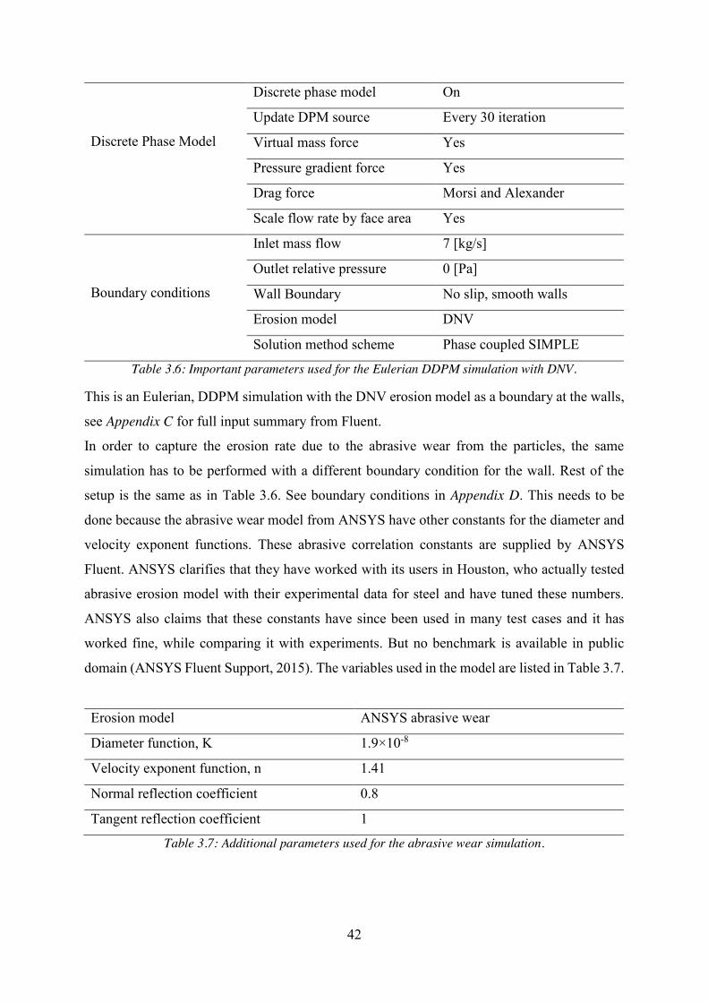
42

Discrete Phase Model

Discrete phase model On

Update DPM source Every 30 iteration

Virtual mass force Yes

Pressure gradient force Yes

Drag force Morsi and Alexander

Scale flow rate by face area Yes

Boundary conditions

Inlet mass flow 7 [kg/s]

Outlet relative pressure 0 [Pa]

Wall Boundary No slip, smooth walls

Erosion model DNV

Solution method scheme Phase coupled SIMPLE

Table 3.6: Important parameters used for the Eulerian DDPM simulation with DNV.

This is an Eulerian, DDPM simulation with the DNV erosion model as a boundary at the walls,

see Appendix C for full input summary from Fluent.

In order to capture the erosion rate due to the abrasive wear from the particles, the same

simulation has to be performed with a different boundary condition for the wall. Rest of the

setup is the same as in Table 3.6. See boundary conditions in Appendix D. This needs to be

done because the abrasive wear model from ANSYS have other constants for the diameter and

velocity exponent functions. These abrasive correlation constants are supplied by ANSYS

Fluent. ANSYS clarifies that they have worked with its users in Houston, who actually tested

abrasive erosion model with their experimental data for steel and have tuned these numbers.

ANSYS also claims that these constants have since been used in many test cases and it has

worked fine, while comparing it with experiments. But no benchmark is available in public

domain (ANSYS Fluent Support, 2015). The variables used in the model are listed in Table 3.7.

Erosion model ANSYS abrasive wear

Diameter function, K 1.9×10-8

Velocity exponent function, n 1.41

Normal reflection coefficient 0.8

Tangent reflection coefficient 1

Table 3.7: Additional parameters used for the abrasive wear simulation.

43

For simulation (Number 3), the procedure is the same as described for the straight pipe except

for the flow conditions that are different for the Bean Choke.

3.2.3 Post processing for Eulerian modeling The fully coupled simulations with DDPM as an Eulerian parameter are also post processed in

ANSYS Fluent. The erosion rate calculations are divided into two parts; one part consists of

the erosion rate calculations from particles impinging the walls, the procedure are the same as

with the DPM simulation in chapter 3.1.3. The other part is a calculation method that is based

on the wall shear stress of particles sliding along the wall. In order to capture the abrasive wear

from the slurry flow in both the straight pipe and the bean choke, another custom erosion rate

function has to be defined which includes the solid wall shear stress. The function is based on

ANSYS’s abrasive model, but the first two variables, the constant K and particle velocity V,

are included in the wall boundary condition. So, the abrasive wear addition is calculated as

follows:

> @

6

3

( _ _ ) 10/

7800 /

sws

spabrasive

particles

DPM erosion rateER m kg

kg m m

DWD

P

§ ·� � �¨ ¸¨ ¸

© ¹ ª º �¬ ¼

(3.2)

where,

wsW is the particle wall shear stress,

(DPM_erosion_rate) is the KVn values from the definition,

sD is the particle volume fraction and

spD is the Packing volume fraction.

particlesm is the mass flowrate of particles for a given case and 7800 is the density of steel.

All these values are calculated within the simulation and the values are therefore taken straight

from Fluent when this is computed. The erosion rate results are then plotted in Fluent, and

written to an excel file. Then, for the bean choke simulations (Number 3), both the DDPM-

DNV and DDPM-Abrasive simulation results are summarized to give the total erosion rate,

which is represented by equation (3.3).

> @/total impact abrasiveER m kg ER ERP � (3.3)

44

3.3 Simulations with DEM collision model DPM with DEM collision model:

The DEM collision model is possible to include with the DPM model even though it is suited

for simulations with higher particle loading where the particle-particle interaction is more

important than in the DPM simulation. In this thesis, the DEM is included in a DPM simulation

to see how it effects the erosion rate results, and if the combination is possible/usable at all. A

Lagrangian DPM is cheaper than an Eulerian approach, and therefore it would be interesting to

investigate the possibility to include DEM in DPM simulation on both high and low particle

loading.

DDPM with DEM collision model:

For the Eulerian model with DDPM, the DEM collision model is included for its purpose, which

is to include the particle-particle interaction in a slurry flow with higher particle loading. This

simulation requires very complex calculations and therefore require loads of memory. The

computational cost is high, and to run it on a normal computer is difficult.

In both simulations above, not much had to be changed in the original setup in order to include

DEM collision model. The procedure in Fluent is as follows:

1. In the Discrete Phase Model setup in Fluent, DEM is enabled under the physical models

tab.

2. Fluent then requires a particle time step for the unsteady and implicit particle tracking.

3. Under DEM collision laws, the collision pairs for particle-particle and particle-wall is

defined by selecting two available contact force laws which is the spring-constant, K

and friction constant εD.

4. In the injection properties, the DEM collision partner is chosen.

5. The last part when defining DEM collision partner is within the boundary conditions at

inlet, wall and outlet. DEM is chosen under DPM to the wall material as collision

partner.

45

4. Results and Discussion This chapter will present the results from the simulations and the general discussion about them.

The simulations will be presented in the same order as in Chapter 3, and with the results as

mentioned in Table 4.1:

4.1 The results from the Bean Choke simulation (Number 1) are presented, discussed

and results are compared with the experimental data from the DNV paper.

4.2 The Eulerian DDPM simulation results (Number 2) regarding the distribution of

sand particles through the straight pipe are presented and discussed. Results from the

Eulerian DDPM simulation on the Bean Choke are presented (Number 3) and compared

to the Lagrangian DPM simulation (Number 1).

4.3 The simulations including the DEM collision model are discussed (Number 4).

4.1 Validation of the DNV impact erosion model The results for the Bean Choke case have been very dependent on the mesh quality. In order to

get a converged solution, and also get reasonable erosion rate results, the different quality

parameters had to be satisfied. Aspect ratio, orthogonal quality and skewness have been looked

into as important factors when developing a suitable mesh for erosion simulations. It is

important to state that no other mesh independency test was performed on the Bean Choke than

making sure that y+ values was sufficiently low, the quality was good and that the fluid solution

converged. The results from the test show that the ANSA mesh give the best results for the fluid

solution and then also the best result regarding erosion rate. The ANSA mesh results are

therefore the ones that are presented in this thesis.

The solution of the fluid over the contraction is shown in Figure 4.1, from simulation (Number

1).

Number Multiphase Parameter Erosion Model Geometry Result

1 DPM DNV Bean Choke Erosion Rate

2 DDPM DNV+Abrasive Straight-pipe Particle Distribution

3 DDPM DNV+Abrasive Bean Choke Erosion Rate

4 DEM DNV+Abrasive Bean Choke Erosion Rate

Table 4.1: Overview of simulations

46

As seen from the legend on the left side in Figure 4.1, the velocity is increasing significantly as

passing through the contraction, ending up with close to 100 [m/s]. The red arrows indicates

where the flow is reversed after the 45° angle increase. For this simulation, the y+ values are

sufficiently low, and less than 5. This means that the turbulence models solves the flow close

to the wall. Figure 4.2 to shows the y+ values from the simulation showing that the transition to

the small pipe is the most exposed area, and is expected since this area has the highest velocity.

Figure 4.1: Fluid solution over the contraction.

Figure 4.2: Contour of y+ values in the cell layer closest to the wall.

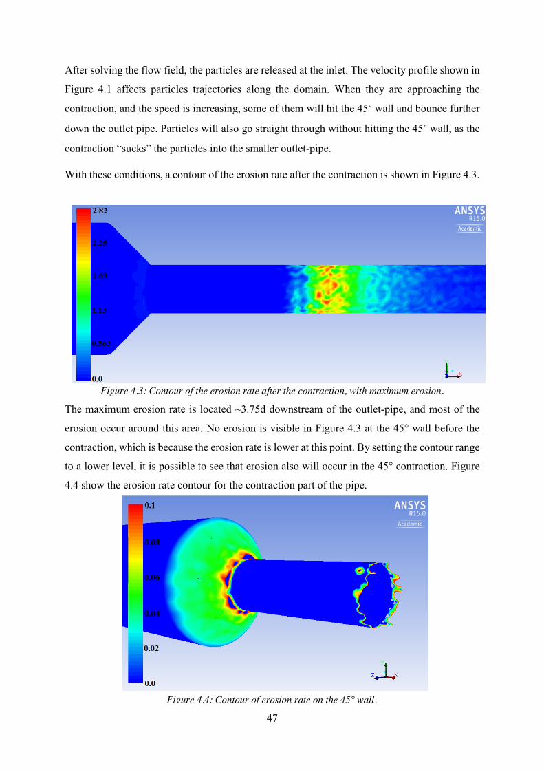
47

After solving the flow field, the particles are released at the inlet. The velocity profile shown in

Figure 4.1 affects particles trajectories along the domain. When they are approaching the

contraction, and the speed is increasing, some of them will hit the 45° wall and bounce further

down the outlet pipe. Particles will also go straight through without hitting the 45° wall, as the

contraction “sucks” the particles into the smaller outlet-pipe.

With these conditions, a contour of the erosion rate after the contraction is shown in Figure 4.3.

The maximum erosion rate is located ~3.75d downstream of the outlet-pipe, and most of the

erosion occur around this area. No erosion is visible in Figure 4.3 at the 45° wall before the

contraction, which is because the erosion rate is lower at this point. By setting the contour range

to a lower level, it is possible to see that erosion also will occur in the 45° contraction. Figure

4.4 show the erosion rate contour for the contraction part of the pipe.

Figure 4.3: Contour of the erosion rate after the contraction, with maximum erosion.

Figure 4.4: Contour of erosion rate on the 45° wall.

48

The different impact velocities for the particles can explain the different erosion rate

magnitudes on the wall, which is almost ten times higher after the contraction. The impact

angles are also different, and as the DNV impact function in Figure 2.6 in chapter 2.2.1 show,

will the maximum erosion occur at 15°-30° (DNV, 2007, p. 12), which is the case after the

contraction.

Erosion rate along the pipe section is the most important result of this simulation, since the

experiment report the erosion rate from the contraction and downstream the smallest pipe. The

results from the simulation are plotted against the experimental data in Figure 4.5.

The black line represent the experimental results from DNV (Huser & Kvernvold, 1998, pp. 5-

6). In the experimental paper, it is not mentioned if these values are average or maximum

erosion rates, so the simulation results are presented with both the maximum (red line) and

average (the blue line) values at given distance after the contraction for comparison.

Results are slightly off compared with the experiment considering the location of maximum

erosion rate, which is approximately 0.02m i.e. ~1d downstream of the pipe from where the

experiment registered it. The maximum average result from the simulation is a bit lower than

the experiment, while the maximum show almost the same value.

Figure 4.5: Result of the DPM simulation.

49

Simulations have also been performed on a geometry without the sharp edge in the end of the

contraction to reduce the backflow and to see how this affect the erosion rate results, and the

location of the maximum erosion rate. This should reduce the swirl after the contraction, which

it also does for the fluid simulation. When particles are sent through the domain, the distance

from the contraction to the maximum erosion is still the same. Since the fluid affects the

particles, and not the other way around with this Lagrangian approach, the particles are exposed

to the swirls without affecting it. In the experiment, where the particles also affect the fluid, this

swirl can be too small to have an effect on the particles flowing through the domain and

therefore they hit the walls at an earlier stage than in the CFD simulations.

What the Fluent results do show, is the same erosion rate pattern as in the experiment; with one

big “bump” straight after the contraction, and a slow decrease until 0.2m. After this location,

the experiment registers some erosion on the pipe wall further downstream, which is not

registered in the Fluent simulations. This has to do with the DPM which only capture the

particles impinging the wall due to changes in flow directions etc. The model does not capture

the particles sliding and jumping along the wall.

As seen in Figure 4.5, the experiment from DNV only show 11 points along the pipe where

erosion rate are reported, which is few. In general, more details should have been given in the

DNV paper about how and whether the geometry changed during the tests. Of course, there are

many parameters that should be investigated further for the experiment, for example particle

size variations, particle deformation during experiment, particle tracking with lasers etc. These

parameters are not discussed in the DNV paper, and is therefore not be discussed any further in

this thesis.

Simulations on the Bean Choke have also been performed with a two-way coupled Lagrangian

approach to see if it had effect on the results. The continuous fluid is then solved while the

particles are sent through the domain every 25th iteration. This means that the phases are

coupled, since the particles affect the continuum in a way that they are sent through at different

stages of the calculation. The result of these simulations are not any better than the one-way

coupled, standard approach, and therefore not discussed any further.

50

4.2 Eulerian model with DDPM

With the validation of the DNV erosion model against the experimental data, the model can be

used for further simulations within the Eulerian model with DDPM. In this part of the thesis,

the results from the Alberta case were supposed to be used as validation for the Eulerian DDPM

in Fluent for prediction erosion in slurry-flow systems. This is the only case found in literature

that reports erosion rate results with higher particle loading. After replicating the case, and

performing several simulations in order to get good results, it has come to the writer’s attention

that there will be a problem with the test material in the Alberta case, which is the urethane

coated pipe walls. The problem is within the DPM model, which also is a part of the DDPM

model; The DNV erosion model uses material constants, which are the velocity exponent

function n, and the diameter coefficient, K, as, described in chapter 2.2.1 in equation 2.5. These

are determined by experimental investigations, and are given for a small range of metals. The

coating used in the Alberta case is urethane, which is a polymer and not a metal, and there are

therefore no data in literature that can be used as material constants for this coating. Since these

are very sensitive values for the erosion calculation, they have to be correct. With such a

problem, the Alberta case is not suitable as a validation case when it comes to slurry erosion.

The experiment does also show results regarding the flow field and the particle distribution.

With the result from the different DDPM simulations on the straight pipe experiment from

Alberta, it should be possible to plot these profiles and compare the flow field from Fluent with

the experiment. If this shows good agreement, the erosion rate calculation on the steel pipe

should assumed to be as given. This is not a procedure to validate the Eulerian model regarding

erosion prediction in the slurry flow, but an assumption that if the model can give reliable

simulations of the flow-field, and an indication of how the erosion rate results will be. Due to

time limitations, this procedure was not completed.

Instead the experiment was used to set up the Eulerian DDPM model by focusing on the visible

wear on the bottom pipe wall, and not the magnitude. Because of the gravity affecting the high

concentrated particle flow, particles are as mentioned sliding and jumping along the pipe wall.

It should be possible to set up a simulation and get the erosion rate results on the bottom wall,

even on a steel pipe.

With this setup for the straight pipe (Number 2), Eulerian DDPM simulations are performed on

the Bean Choke experiment from DNV in order to compare the Lagrangian DPM results with

the Eulerian approach which includes the abrasive wear (Number 3).

51

4.2.1 Straight pipe results

For the straight pipe simulation, with the same particle concentration as in the Alberta

experiment, the distribution of particles over the cross-section along the pipe is shown in Figure

4.6 with particle volume fraction on the legend to the left. This figure show that particles are

located close to the bottom wall due to the gravitational forces in the –Y direction acting on

them, which is also the result in the experiment.

This distribution of the particles are as expected when looking at the simulation results

compared with the experiment (Loewen, 2013, pp. 102-108). The slurry flow in this case can

be described as a settling, heterogeneous slurry flow. The momentum transfer between the

particles, fluid and the walls will behave as described in chapter 2.1.3.

Figure 4.6: Particle distribution along the straight pipe.

52

The wear from the sliding particles occurs at the bottom pipe wall, and the erosion rate results

from Fluent is distributed as shown in Figure 4.7:

A Lagrangian DPM simulation setup was also performed on the straight pipe with high particle

concentration. Results show that the pipe-walls are not exposed to erosion, which is expected

from the impact based method. This is a simple geometry where the fluid do not change

direction, and therefore the particles will not impact the walls and the model will not capturing

the erosion.

4.2.2 Eulerian simulations on DNV’s Bean Choke After setting up the Eulerian model on the straight pipe, and starting to understand how it works,

the model was tested on the Bean Choke case with different particle loadings in order to see the

effect on the erosion rate when the abrasive wear becomes more dominant than at a lower level

of particle loading. The DPM simulation result as discussed in chapter 4.1 is used to compare

with the DDPM results with total erosion rate, and is shown in Figure 4.8 on the next page.

Figure 4.7: Contour of erosion rate along the pipe.

53

Figure 4.8: Plot of the results with different particle loading with DDPM and the DPM.

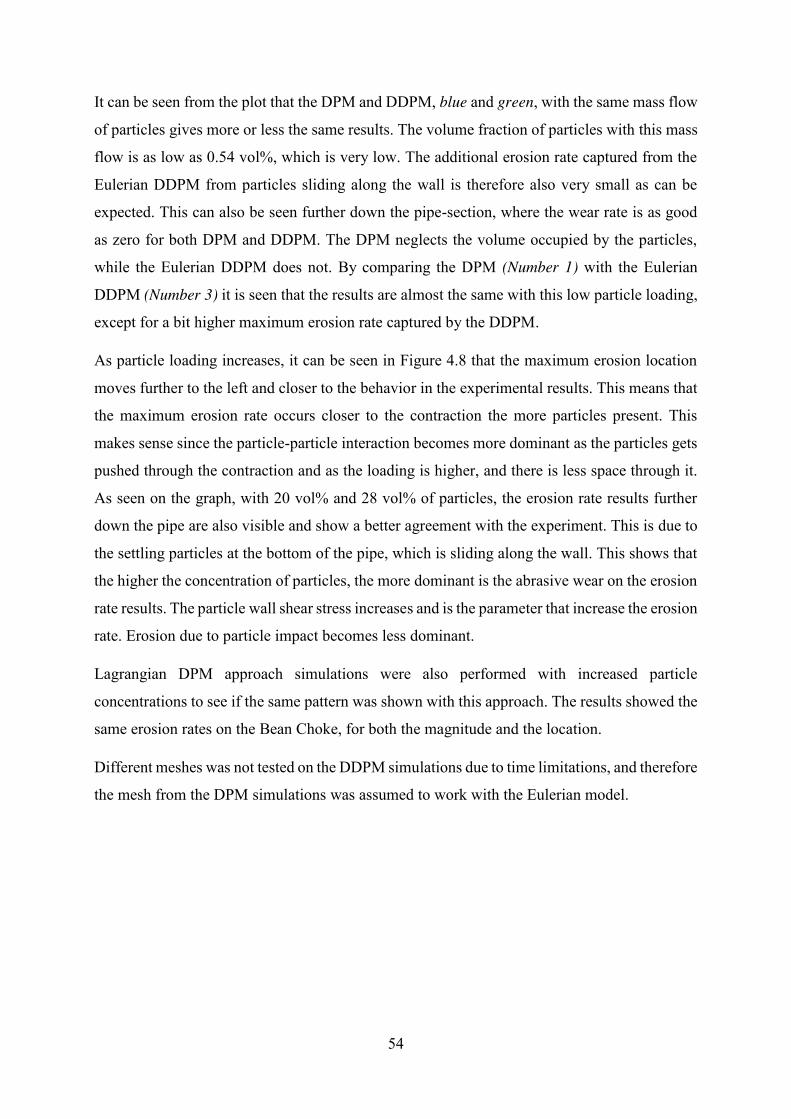
54

It can be seen from the plot that the DPM and DDPM, blue and green, with the same mass flow

of particles gives more or less the same results. The volume fraction of particles with this mass

flow is as low as 0.54 vol%, which is very low. The additional erosion rate captured from the

Eulerian DDPM from particles sliding along the wall is therefore also very small as can be

expected. This can also be seen further down the pipe-section, where the wear rate is as good

as zero for both DPM and DDPM. The DPM neglects the volume occupied by the particles,

while the Eulerian DDPM does not. By comparing the DPM (Number 1) with the Eulerian

DDPM (Number 3) it is seen that the results are almost the same with this low particle loading,

except for a bit higher maximum erosion rate captured by the DDPM.

As particle loading increases, it can be seen in Figure 4.8 that the maximum erosion location

moves further to the left and closer to the behavior in the experimental results. This means that

the maximum erosion rate occurs closer to the contraction the more particles present. This

makes sense since the particle-particle interaction becomes more dominant as the particles gets

pushed through the contraction and as the loading is higher, and there is less space through it.

As seen on the graph, with 20 vol% and 28 vol% of particles, the erosion rate results further

down the pipe are also visible and show a better agreement with the experiment. This is due to

the settling particles at the bottom of the pipe, which is sliding along the wall. This shows that

the higher the concentration of particles, the more dominant is the abrasive wear on the erosion

rate results. The particle wall shear stress increases and is the parameter that increase the erosion

rate. Erosion due to particle impact becomes less dominant.

Lagrangian DPM approach simulations were also performed with increased particle

concentrations to see if the same pattern was shown with this approach. The results showed the

same erosion rates on the Bean Choke, for both the magnitude and the location.

Different meshes was not tested on the DDPM simulations due to time limitations, and therefore

the mesh from the DPM simulations was assumed to work with the Eulerian model.

55

4.3 DEM collision model After performing both the DPM and the Eulerian DDPM simulations, the same simulations

were performed with the DEM collision model activated. Several tries have been done in order

to include the method but without luck. The method is a new simulation methodology, and not

much is known in literature about how it works within these models. The simulations were

performed on a normal computer which was very slow and after only ten iterations divergence

was reported in the solution. Simulation attempts were made a High Performance Cluster in

order to see if this could give any results. This also took too long, and did not give any good

result within the time frame of this thesis.

56

5. Conclusion In this thesis, erosion analysis were performed using ANSYS Fluent on flow containing

different particle loadings. The simulation process was performed as follows:

1. The DNV erosion model was validated against an experimental case with low particle

concentration. This simulation was performed by the use of the Lagrangian Discrete

Phase Model (DPM) approach.

2. A Slurry flow-case simulation with the Eulerian model with a Dense Discrete Phase

Model (DDPM) was set up using the flow condition results from a straight pipe

experiment.

3. The same Eulerian DDPM setup was then used to simulate the Bean Choke in order to

see if the model could capture the abrasive wear from the particles. All results from the

above simulations were written to file, plotted in Matlab and compared with

experimental results.

4. Attempts were made in order to include the DEM collision model into the erosion

simulations.

Results from the DNV erosion model show good agreement with the experimental data for the

Bean Choke. This model was therefore used further in the thesis within the Eulerian DDPM

simulation. Even though the straight pipe could not be used as a validation case for erosion

study, the Eulerian DDPM simulations show good agreement with the experiments flow

conditions. The setup was then used to simulate a fully coupled Euler-Euler simulation on the

Bean Choke. The abrasive wear results with the low particle concentration did not differ much

from the DPM simulation. Comparing the DPM simulation (Number 1) with the Eulerian

DDPM (Number 3) it is reasonable to use the Lagrangian DPM approach for cases with low

particle loading. This method is cheaper when talking about computational cost, and requires

less memory.

However, as the particle concentration was increased, it was evident that the Eulerian DDPM

captured the abrasive wear from particles sliding and bouncing along the wall downstream the

pipe after the contraction. This erosion rate could be calculated by the wall shear stress from

the particles, which was increasing with the concentration.

It should be mentioned that the Eulerian DDPM is a new simulation methodology, and few

investigations has so far been reported with this Eulerian parameter regarding erosion. Not even

ANSYS have any validated erosion studies available with this model. Therefore, without

57

comparing the results from the simulations with higher particle loading with any experimental

data, it is hard to draw a conclusion except from that the model capture the abrasive wear from

the slurry flows as the wall shear stress from the particles increases.

When the particle concentration was increased in the DPM simulations, the results did not

change much. This show that the impact based erosion models, which neglects the occupied

volume of the particle, do not capture the additional abrasive erosion caused by higher particle

loading, as the Eulerian DDPM do.

Several attempts were made in order to include the DEM collision model into the simulations

in order to capture more of the particle-particle interactions. This method proved to be

extremely memory consuming and too computational costly in order to perform on a normal

computer. An attempt on a High Performance Cluster was also made but without any luck. This

method is very complex and is not recommended to use for these types of simulations.

58

6. Recommendations for Further Work The Eulerian model with the DDPM parameter should be validated against experimental data

which gives reliable erosion rate results. More time should be spent on searching for available

experimental results with higher particle concentration in literature. A suggestion would be to

contact the publishers directly and get their experience with both the experiments and the

available cases on the topic.

The ideal way for validation of the Eulerian DDPM model regarding erosion, would be if the

same person that is doing the simulation case in CFD also performs the experiment. With this

approach, it could be possible to include the effects of several important parameters to both the

experiment and CFD simulations. Some of them are:

- Particle size and shape distribution

- Variation of particle loading

- Wall roughness

For the simulation part of this study, the mesh development process should be expanded in

order to make sure that the results for the Eulerian simulation got mesh independent. Not much

is reported in literature about how coarse or fine a mesh should be for an Eulerian fluid-particle

simulation. To develop an ideal mesh can be crucial for the results.

Erosion studies, both impact based and slurry, should also be performed using different CFD

programs. Both in order to compare different models in different programs, and also to look for

the ideal CFD code to predict erosion.

59

7. References

ANSYS Fluent Support (2015).

ANSYS Help Viewer (2013). ANSYS Help Viewer, Verison 15.0.0.

Bredberg, J. (2000). ‘On the Wall Boundary Condition for Turbulence Models’, Chalmers Internal Report 00/4. pp. 11-12. Available at: http://www.tfd.chalmers.se/~lada/postscript_files/jonas_report_WF.pdf (29.10.2014)

Brown, N.P. & Heywood, N.I. (1991). Slurry Handling: Design of Solid-Liquid Systems.

Essex: Elsevier Science Publishers LTD.

Cundal P.A. & Strack O.D.L. (1979). ‘A Discrete Numerical model for Granular Assemblies’, Geotechnique, Vol. 29. (no. 1), pp. 47-65. Available at: http://www.icevirtuallibrary.com/content/article/10.1680/geot.1979.29.1.47 (11.03.2015)

Det Norske Veritas. (2007). RP O501 – Revision 4.2. Erosive Wear in Piping Systems. Høvik:

Det Norske Veritas. Dosanjh, S. & Humphrey, J. A. C. (1985). ‘The influence of turbulence on erosion by a

particle-laden fluid jet’, Wear, vol. 102 (no. 4) pp. 309-330. Available at: http://www.sciencedirect.com/science/article/pii/0043164885901759 (20.03.2015)

Eltvik, M. (2013). Sediment erosion in Francis Turbines. Doctoral Thesis. Norwegian

University of Science and Technology, Trondheim. Gillies R. G. (1993). Pipeline flow of coarse particle slurries. Master’s Thesis. University of

Saskatchewan, Saskatoon. Available at: http://ecommons.usask.ca/bitstream/handle/10388/etd-03242009-142017/Gillies_Randall_G._1993.pdf?sequence=1 (15.02.2015)

Huser, A. & Kvernvold, O. (1998). Prediction of Sand Erosion in Process and Pipe

Components. Høvik: Det Norske Veritas. ISO 14688-1 (2002) Geotechnical investigation and testing – Identification and classification

of soil. King, R. P. (2002). Introduction to Practical Fluid Flow. Salt Lake City: Elsevier Ltd.

Available at: http://www.sciencedirect.com/science/book/9780750648851 (01.04.2015)

Kosel, T.H. (1992). ‘Solid Particle Erosion’, ASM Handbook, Vol. 18, pp. 199-213. Available

at: http://app.knovel.com/web/toc.v/cid:kpASMHVFL2/viewerType:toc/root_slug:asm-handbook-volume-18/url_slug:kt007PXRS6 (13.03.2015)

Loewen, D. J. (2013). Characterization of Wear in a Laboratory-Scale Slurry Pipeline.

Master’s Thesis. University of Alberta, Alberta. Available at:

60

https://era.library.ualberta.ca/public/view/item/uuid:5f9bcae0-1af0-4097-b62d-d4858a444938/ (18.02.2015)

Mali, T, Khudabadi, V, Rana, A.S, Vijay, A. & Adarsh, M.R. (2014). Slurry-Flow Pressure

Drop in Pipes with Modified Wasp Method. SME Annual Meeting/Exhibit. Salt Lake City.

Meng, H.C. & Ludema, K.C. (1995). ‘Wear models and predictive equations: their form and

content’, Wear, vol. 181-183, pp. 443-457. Available at: http://www.sciencedirect.com/science/article/pii/0043164895901582 (10.02.2015)

Morsi S. A. & Alexander A. J. (1972). ‘An investigation of particle trajectories in two-phase

flow systems’, J. Fluid Mech. Vol. 55 (part 2), pp. 193-208. Available at: http://journals.cambridge.org/download.php?file=%2FFLM%2FFLM55_02%2FS0022112072001806a.pdf&code=cf7e344ae55d4a9cb810d4d41529542f (19.04.2015)

Roitto V. (2014). Slurry Flows in Metallurgical Process Engineering – Development of Tools

and Guidelines. Master’s Thesis. Aalto University, Aalto. Available at: https://aaltodoc.aalto.fi/bitstream/handle/123456789/13113/master_Roitto_Ville_2014.pdf?sequence=1 (06.03.2015)

Shook, C. A. & Roco, M. C. (1991). Slurry Flow: Principles and Practice. USA:

Butterworth-Henemann. Slater, J.W. (2008). Tutorial on CFD Verification and Validation. Available at: http://www.grc.nasa.gov/WWW/wind/valid/tutorial/tutorial.html (15.10.2014)

Versteeg, H.K. & Malalasekera, W. (1995). An introduction to Fluid Dynamics: The Finite Volume Method. England: Longman Scientific & Technical.

Wasp, E. J. (1977). Solid-liquid flow - Slurry Pipeline Transportation. Series on Bulk Material handling Vol. 1. Germany: Trans Tech Publications.

White, F.M. (1999). Fluid Mechanics. Fourth Edition. Singapore: McGraw-Hill Book Co.

Wood, R.J.K, Jones, T.F, Miles, N.J. & Ganeshalingham, J. (2001). ‘Upstream swirl-induction for reduction of erosion damage from slurries in pipeline bends’ Wear, vol. 25 (no. 1-12), pp. 770-778. Available at: http://www.sciencedirect.com/science/article/pii/S0043164801007153 (01.02.2015)

Zikanov, O. (2010). Essential Computational Fluid Dynamics. New Jersey: John Wiley &

Sons, Inc.

61

Appendices Appendix A

ANSYS Meshing

Several attempts were made using the ANSYS Meshing to mesh the domain. Two different

meshing methods with the ANSYS meshing methods were used; the sweep method, which is a

hex-mesh, and the tetra-mesh method:

1. The sweep method have an advantage that it is easy to keep control of the number of cells in

each section along the pipe with a structured hex-mesh and inflation layers. Face size is defined

at the inlet and goes through the whole domain. Edge-sizing was used to give better mesh

quality regarding orthogonal quality and aspect ratio, but without luck. See Figure 3.1. for the

sweep-mesh from ANSYS Meshing.

2. The tetra-mesh is much more unorganized, and more difficult to get control over the

important quality aspects. With hex-cells in the inflation layers, the transition to the tetra-cells

reduces the mesh quality. Also with its nodes-element ratio of 1:3, converged solutions is

difficult to obtain. The mesh is shown in Figure 3.2.

Hex mesh from ANSYS Meshing.

Tetra mesh from ANSYS Meshing.

62

Appendix B

DPM Simulation in Fluent – Input Summary

Fluent Version: 3d, dp, pbns, sstkw (3d, double precision, pressure-based, SST k-omega) Release: 15.0.0 Title: Models ------ Model Settings --------------------------------------------------------- Space 3D Time Steady Viscous SST k-omega turbulence model Heat Transfer Disabled Solidification and Melting Disabled Species Disabled Coupled Dispersed Phase Enabled NOx Pollutants Disabled SOx Pollutants Disabled Soot Disabled Mercury Pollutants Disabled Material Properties ------------------- Material: sand (inert-particle) Property Units Method Value(s) ------------------------------------------------- Density kg/m3 constant 2600 Cp (Specific Heat) j/kg-k constant 1680 Material: air/co2 (fluid) Property Units Method Value(s) --------------------------------------------------------------- Density kg/m3 constant 24.136169 Cp (Specific Heat) j/kg-k constant 1006.43 Thermal Conductivity w/m-k constant 0.0242 Viscosity kg/m-s constant 1.5e-05 Molecular Weight kg/kgmol constant 28.966 Reference Temperature k constant 309 Thermal Expansion Coefficient 1/k constant 0 Speed of Sound m/s none #f Material: aluminum (solid) Property Units Method Value(s) --------------------------------------------------- Density kg/m3 constant 2719 Cp (Specific Heat) j/kg-k constant 871

63

Thermal Conductivity w/m-k constant 202.4 Boundary Conditions ------------------- Zones name id type ----------------------------- wall 1 wall inlet 2 velocity-inlet outlet 3 pressure-outlet Setup Conditions wall Condition Value ------------------------------------------------------------------------------------------------------------------------------------------------------------------------------------------------------------------------------------------------------------------------------------------------------------------------------------------------------------------------------------------------------------------------------------------------------------------------ Enable shell conduction? no Wall Motion 0 Shear Boundary Condition 0 Define wall motion relative to adjacent cell zone? yes Apply a rotational velocity to this wall? no Velocity Magnitude (m/s) 0 X-Component of Wall Translation 1 Y-Component of Wall Translation 0 Z-Component of Wall Translation 0 Define wall velocity components? no X-Component of Wall Translation (m/s) 0 Y-Component of Wall Translation (m/s) 0 Z-Component of Wall Translation (m/s) 0 Wall Roughness Height (m) 0 Wall Roughness Constant 0.5 Discrete Phase BC Type 2 Normal 0.80000001 Tangent 1 Discrete Phase BC Function none Impact Angle Function ((polynomial piecewise-linear angle (0 . 0) (0.052359872 . 0.38931575) (0.10471974 . 0.62559682) (0.17453291 . 0.79820257) (0.23911008 . 0.87917018) (0.29670593 . 0.92019415) (0.40666166 . 0.9651503) (0.52359873 . 0.99254328) (0.6352998 . 1.0018587) (0.69813162 . 0.99890703) (0.87266451 . 0.96232015) (1.0471975 . 0.89367861) (1.2217304 . 0.79614067) (1.3962632 . 0.67655677) (1.5707961 . 0.56851071))) Diameter Function ((polynomial diameter 1.9999999e-09)) Velocity Exponent Function ((polynomial normal-velocity 2.5999999)) Rotation Speed (rad/s) 0

64

X-Position of Rotation-Axis Origin (m) 0 Y-Position of Rotation-Axis Origin (m) 0 Z-Position of Rotation-Axis Origin (m) 0 X-Component of Rotation-Axis Direction 0 Y-Component of Rotation-Axis Direction 0 Z-Component of Rotation-Axis Direction 1 X-component of shear stress (pascal) 0 Y-component of shear stress (pascal) 0 Z-component of shear stress (pascal) 0 Fslip constant 0 Eslip constant 0 Specularity Coefficient 0 Enable Thermal Stabilization? no Scale Factor 0 Stabilization Method 1 inlet Condition Value ---------------------------------------------------- Velocity Specification Method 2 Reference Frame 0 Velocity Magnitude (m/s) 11.4 Supersonic/Initial Gauge Pressure (pascal) 1410000 Coordinate System 0 X-Velocity (m/s) 0 Y-Velocity (m/s) 0 Z-Velocity (m/s) 0 X-Component of Flow Direction 1 Y-Component of Flow Direction 0 Z-Component of Flow Direction 0 X-Component of Axis Direction 1 Y-Component of Axis Direction 0 Z-Component of Axis Direction 0 X-Coordinate of Axis Origin (m) 0 Y-Coordinate of Axis Origin (m) 0 Z-Coordinate of Axis Origin (m) 0 Angular velocity (rad/s) 0 Turbulent Specification Method 3 Turbulent Kinetic Energy (m2/s2) 1 Specific Dissipation Rate (1/s) 1 Turbulent Intensity (%) 5 Turbulent Length Scale (m) 1 Hydraulic Diameter (m) 0.054 Turbulent Viscosity Ratio 10 Discrete Phase BC Type 4 Discrete Phase BC Function none is zone used in mixing-plane model? no outlet Condition Value ----------------------------------------------------------- Gauge Pressure (pascal) 0 Backflow Direction Specification Method 1 Coordinate System 0 X-Component of Flow Direction 1 Y-Component of Flow Direction 0

65

Z-Component of Flow Direction 0 X-Component of Axis Direction 1 Y-Component of Axis Direction 0 Z-Component of Axis Direction 0 X-Coordinate of Axis Origin (m) 0 Y-Coordinate of Axis Origin (m) 0 Z-Coordinate of Axis Origin (m) 0 Turbulent Specification Method 3 Backflow Turbulent Kinetic Energy (m2/s2) 1 Backflow Specific Dissipation Rate (1/s) 1 Backflow Turbulent Intensity (%) 2.9999999 Backflow Turbulent Length Scale (m) 1 Backflow Hydraulic Diameter (m) 0.02 Backflow Turbulent Viscosity Ratio 10 Discrete Phase BC Type 4 Discrete Phase BC Function none is zone used in mixing-plane model? no Radial Equilibrium Pressure Distribution no Average Pressure Specification? no 0 Specify targeted mass flow rate no Targeted mass flow (kg/s) 1 Upper Limit of Absolute Pressure Value (pascal) 5000000 Lower Limit of Absolute Pressure Value (pascal) 1 Solver Settings --------------- Equations Equation Solved ------------------- Flow yes Turbulence yes Numerics Numeric Enabled --------------------------------------- Absolute Velocity Formulation yes Relaxation Variable Relaxation Factor --------------------------------------------- Pressure 0.3 Density 1 Body Forces 1 Momentum 0.7 Turbulent Kinetic Energy 0.8 Specific Dissipation Rate 0.8 Turbulent Viscosity 1 Discrete Phase Sources 0.5 Linear Solver Solver Termination Residual Reduction

66

Variable Type Criterion Tolerance ----------------------------------------------------------------------- Pressure V-Cycle 0.1 X-Momentum Flexible 0.1 0.7 Y-Momentum Flexible 0.1 0.7 Z-Momentum Flexible 0.1 0.7 Turbulent Kinetic Energy Flexible 0.1 0.7 Specific Dissipation Rate Flexible 0.1 0.7 Pressure-Velocity Coupling Parameter Value ------------------ Type SIMPLE Discretization Scheme Variable Scheme ----------------------------------------------- Pressure Second Order Momentum Second Order Upwind Turbulent Kinetic Energy First Order Upwind Specific Dissipation Rate First Order Upwind Solution Limits Quantity Limit --------------------------------------- Minimum Absolute Pressure 1 Maximum Absolute Pressure 5e+10 Minimum Temperature 1 Maximum Temperature 5000 Minimum Turb. Kinetic Energy 1e-14 Minimum Spec. Dissipation Rate 1e-20 Maximum Turb. Viscosity Ratio 100000

67

Appendix C

DDPM Simulation in Fluent with DNV – Input Summary

Fluent Version: 3d, dp, pbns, eulerian, rke (3d, double precision, pressure-based, Eulerian, realizable k-epsilon) Release: 15.0.0 Title: Models ------ Model Settings ------------------------------------------------------------------- Space 3D Time Steady Viscous Realizable k-epsilon turbulence model Wall Treatment Standard Wall Functions Multiphase k-epsilon Models Mixture k-epsilon Heat Transfer Disabled Solidification and Melting Disabled Species Disabled Coupled Dispersed Phase Enabled NOx Pollutants Disabled SOx Pollutants Disabled Soot Disabled Mercury Pollutants Disabled Material Properties ------------------- Material: sand (inert-particle) Property Units Method Value(s) ------------------------------------------------- Density kg/m3 constant 2600 Cp (Specific Heat) j/kg-k constant 1680 Material: air/co2 (fluid) Property Units Method Value(s) --------------------------------------------------------------- Density kg/m3 constant 24.136169 Cp (Specific Heat) j/kg-k constant 1006.43 Thermal Conductivity w/m-k constant 0.0242 Viscosity kg/m-s constant 1.5e-05 Molecular Weight kg/kgmol constant 28.966 Reference Temperature k constant 309 Thermal Expansion Coefficient 1/k constant 0 Speed of Sound m/s none #f Material: aluminum (solid) Property Units Method Value(s) ---------------------------------------------------

68

Density kg/m3 constant 2719 Cp (Specific Heat) j/kg-k constant 871 Thermal Conductivity w/m-k constant 202.4 Boundary Conditions ------------------- Zones name id type ----------------------------- wall 1 wall inlet 2 velocity-inlet outlet 3 pressure-outlet Setup Conditions wall Condition Value ------------------------------------------------------------------------------------------------------------------------------------------------------------------------------------------------------------------------------------------------------------------------------------------------------------------------------------------------------------------------------------------------------------------------------------------------------------------------ Enable shell conduction? no Wall Motion 0 Shear Boundary Condition 0 Define wall motion relative to adjacent cell zone? yes Apply a rotational velocity to this wall? no Velocity Magnitude (m/s) 0 X-Component of Wall Translation 1 Y-Component of Wall Translation 0 Z-Component of Wall Translation 0 Define wall velocity components? no X-Component of Wall Translation (m/s) 0 Y-Component of Wall Translation (m/s) 0 Z-Component of Wall Translation (m/s) 0 Wall Roughness Height (m) 0 Wall Roughness Constant 0.5 Discrete Phase BC Type 2 Normal 0.80000001 Tangent 1 Discrete Phase BC Function none Impact Angle Function ((polynomial piecewise-linear angle (0 . 0) (0.052359872 . 0.38931575) (0.10471974 . 0.62559682) (0.17453291 . 0.79820257) (0.23911008 . 0.87917018) (0.29670593 . 0.92019415) (0.40666166 . 0.9651503) (0.52359873 . 0.99254328) (0.6352998 . 1.0018587) (0.69813162 . 0.99890703) (0.87266451 . 0.96232015) (1.0471975 . 0.89367861) (1.2217304 . 0.79614067) (1.3962632 . 0.67655677) (1.5707961 . 0.56851071))) Diameter Function ((polynomial diameter 1.9999999e-09))

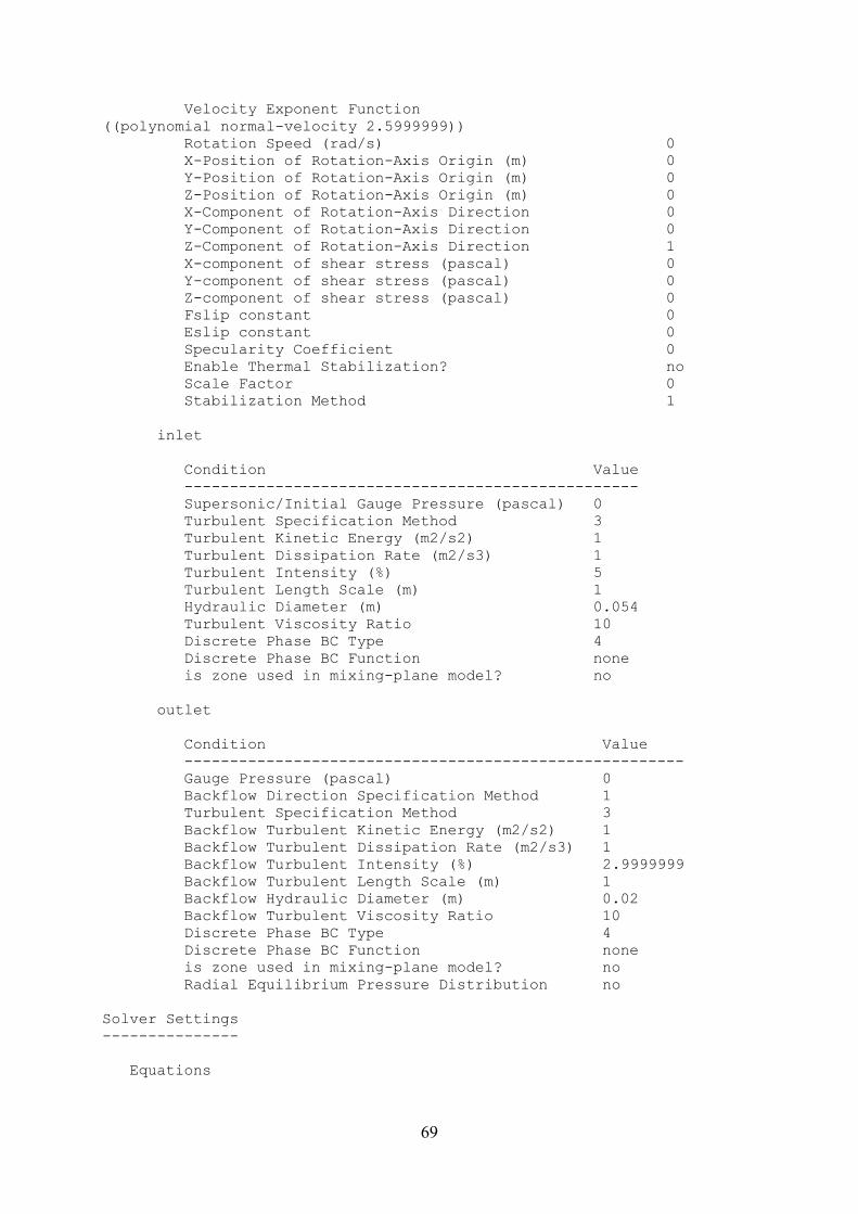
69

Velocity Exponent Function ((polynomial normal-velocity 2.5999999)) Rotation Speed (rad/s) 0 X-Position of Rotation-Axis Origin (m) 0 Y-Position of Rotation-Axis Origin (m) 0 Z-Position of Rotation-Axis Origin (m) 0 X-Component of Rotation-Axis Direction 0 Y-Component of Rotation-Axis Direction 0 Z-Component of Rotation-Axis Direction 1 X-component of shear stress (pascal) 0 Y-component of shear stress (pascal) 0 Z-component of shear stress (pascal) 0 Fslip constant 0 Eslip constant 0 Specularity Coefficient 0 Enable Thermal Stabilization? no Scale Factor 0 Stabilization Method 1 inlet Condition Value -------------------------------------------------- Supersonic/Initial Gauge Pressure (pascal) 0 Turbulent Specification Method 3 Turbulent Kinetic Energy (m2/s2) 1 Turbulent Dissipation Rate (m2/s3) 1 Turbulent Intensity (%) 5 Turbulent Length Scale (m) 1 Hydraulic Diameter (m) 0.054 Turbulent Viscosity Ratio 10 Discrete Phase BC Type 4 Discrete Phase BC Function none is zone used in mixing-plane model? no outlet Condition Value ------------------------------------------------------- Gauge Pressure (pascal) 0 Backflow Direction Specification Method 1 Turbulent Specification Method 3 Backflow Turbulent Kinetic Energy (m2/s2) 1 Backflow Turbulent Dissipation Rate (m2/s3) 1 Backflow Turbulent Intensity (%) 2.9999999 Backflow Turbulent Length Scale (m) 1 Backflow Hydraulic Diameter (m) 0.02 Backflow Turbulent Viscosity Ratio 10 Discrete Phase BC Type 4 Discrete Phase BC Function none is zone used in mixing-plane model? no Radial Equilibrium Pressure Distribution no Solver Settings --------------- Equations

70

Equation Solved ------------------------ Flow yes Volume Fraction yes Turbulence yes Numerics Numeric Enabled --------------------------------------- Absolute Velocity Formulation yes Relaxation Variable Relaxation Factor ---------------------------------------------- Pressure 0.3 Density 1 Body Forces 1 Momentum 0.7 Volume Fraction 0.5 Granular Temperature 0.2 Turbulent Kinetic Energy 0.8 Turbulent Dissipation Rate 0.8 Turbulent Viscosity 1 Discrete Phase Sources 0.5 Linear Solver Solver Termination Residual Reduction Variable Type Criterion Tolerance ------------------------------------------------------------------------ Pressure V-Cycle 0.1 X-Momentum Flexible 0.1 0.7 Y-Momentum Flexible 0.1 0.7 Z-Momentum Flexible 0.1 0.7 Volume Fraction Flexible 0.1 0.7 Turbulent Kinetic Energy Flexible 0.1 0.7 Turbulent Dissipation Rate Flexible 0.1 0.7 Pressure-Velocity Coupling Parameter Value -------------------------------- Type Phase Coupled SIMPLE Discretization Scheme Variable Scheme ----------------------------------------------- Momentum First Order Upwind Volume Fraction First Order Upwind Turbulent Kinetic Energy First Order Upwind Turbulent Dissipation Rate First Order Upwind Solution Limits

71

Quantity Limit --------------------------------------- Minimum Absolute Pressure 1 Maximum Absolute Pressure 5e+10 Minimum Temperature 1 Maximum Temperature 5000 Minimum Turb. Kinetic Energy 1e-14 Minimum Turb. Dissipation Rate 1e-20 Maximum Turb. Viscosity Ratio 100000

72

Appendix D

DDPM Simulation in Fluent with Abrasive – Boundary Conditions

Setup Conditions wall Condition Value ------------------------------------------------------------------------------------------------------------------ Enable shell conduction? no Wall Motion 0 Shear Boundary Condition 0 Define wall motion relative to adjacent cell zone? yes Apply a rotational velocity to this wall? no Velocity Magnitude (m/s) 0 X-Component of Wall Translation 1 Y-Component of Wall Translation 0 Z-Component of Wall Translation 0 Define wall velocity components? no X-Component of Wall Translation (m/s) 0 Y-Component of Wall Translation (m/s) 0 Z-Component of Wall Translation (m/s) 0 Wall Roughness Height (m) 0 Wall Roughness Constant 0.5 Discrete Phase BC Type 2 Normal 0.80000001 Tangent 1 Discrete Phase BC Function none Impact Angle Function ((polynomial piecewise-linear angle (0 . 1) (1.5707961 . 1))) Diameter Function ((polynomial diameter 1.9e-08)) Velocity Exponent Function ((polynomial normal-velocity 1.41)) Rotation Speed (rad/s) 0 X-Position of Rotation-Axis Origin (m) 0 Y-Position of Rotation-Axis Origin (m) 0 Z-Position of Rotation-Axis Origin (m) 0 X-Component of Rotation-Axis Direction 0 Y-Component of Rotation-Axis Direction 0 Z-Component of Rotation-Axis Direction 1 X-component of shear stress (pascal) 0 Y-component of shear stress (pascal) 0 Z-component of shear stress (pascal) 0 Fslip constant 0 Eslip constant 0 Specularity Coefficient 0 Enable Thermal Stabilization? no Scale Factor 0 Stabilization Method 1

73

inlet Condition Value ------------------------------------------------------ Supersonic/Initial Gauge Pressure (pascal) 0 Turbulent Specification Method 3 Turbulent Kinetic Energy (m2/s2) 1 Turbulent Dissipation Rate (m2/s3) 1 Turbulent Intensity (%) 2.9999999 Turbulent Length Scale (m) 1 Hydraulic Diameter (m) 0.054 Turbulent Viscosity Ratio 10 Discrete Phase BC Type 4 Discrete Phase BC Function none is zone used in mixing-plane model? no outlet Condition Value ------------------------------------------------------- Gauge Pressure (pascal) 0 Backflow Direction Specification Method 1 Turbulent Specification Method 3 Backflow Turbulent Kinetic Energy (m2/s2) 1 Backflow Turbulent Dissipation Rate (m2/s3) 1 Backflow Turbulent Intensity (%) 2.9999999 Backflow Turbulent Length Scale (m) 1 Backflow Hydraulic Diameter (m) 0.02 Backflow Turbulent Viscosity Ratio 10 Discrete Phase BC Type 4 Discrete Phase BC Function none is zone used in mixing-plane model? no Radial Equilibrium Pressure Distribution no