Embed Size (px)
Citation preview
Simulation of a Subcritical Power Plant using a BoilerFollowing Control sequence
Carbon Capture and Storage networks
Ricardo Miguel Ferreira Fernandes
Dissertation for the degree of Master of
Chemical Engineering
JuriPresident: Prof. Dr. Sebastiao Manuel Tavares da Silva AlvesSupervisor: Prof. Dr.a Carla Isabel Costa PinheiroCo-Supervisor: Engr. Jose Alfredo Ramos PlasenciaVogal: Dr. Vitor Manuel Vieira Lopes
Dr. Javier Rodriguez
October 2012

Simulation of a Subcritical Power Plant using a BoilerFollowing Control sequence
Carbon Capture and Storage networks
Ricardo Miguel Ferreira Fernandes
Dissertacao para grau de Mestre em
Engenharia Quımica
JuriPresidente: Prof. Dr. Sebastiao Manuel Tavares da Silva AlvesOrientador: Prof. Dr.a Carla Isabel Costa PinheiroCo-Orientador: Engr. Jose Alfredo Ramos PlasenciaVogal: Dr. Vitor Manuel Vieira Lopes
Dr. Javier Rodriguez
Outubro 2012


Anyone who has never made a mistake has never tried anything new.Albert Einstein


Acknowledgments
I would like to thank Prof. Dr. Carla Pinheiro and Engr. Alfredo Ramos, my supervisors, for all
the availability and readiness to help during the internship and thesis development. To Dr. Adekola
Lawal, my direct supervisor, I also want to give a special thanks for the help he gave me during the
work for the thesis. For all the gCCS team I want to say thank you for the close cooperation on the
development of the flowsheets and library models during the 7 months of progress, because without
a team like that the thesis would be even more hard working.
For all the PSE people in general, I want to say that I appreciated the reception and sympathy.
To finish, I would like to thank my family, specially to my girlfriend and mother, for all the support
given to me for being far from home.
iii

Abstract
The objective of this work is to model a pulverized coal power plant and some of its component
units and to apply control based in the boiler following control approach, in order to analyse the
control system and the power plant performance at different operational conditions. The ETI-CCS
project comprises the modelling of the several components of the carbon capture and storage chain,
starting with the pulverized coal power plant, the basis of the thesis.
The modelling is developed in gPROMS and consists building some units to be added to the power
plant library. Some of the models are grabbed from this library to be connected and to represent a
pulverized coal power plant. The building of a flowsheet like the PCPP is a challenge, since the
number of recirculations, between the great number of units, is great.
By controlling the system, it was possible to represent, for example, the typical behaviour of the
key variables of the system in load changes, representing the daily cycle. From the performance
study it was concluded that for lower loads the power plant’s efficiency decreases, consuming more
resources per MW, and that the LHV of the coal and the efficiency of the turbines increase the net
efficiency.
Keywords
Boiler Following Control, Pulverized Coal Power Plant, Carbon Capture and Storage, Modelling,
gPROMS
v

Resumo
O objectivo do trabalho e modelar uma estacao termoelectrica de carvao pulverizado, e algumas
das suas unidades, e aplicar controlo utilizando o modo boiler following, de forma a analisar o controlo
do sistema e a performance da estacao termoeletrica a diferentes condicoes operacionais. O projecto
ETI-CCS inclui a modelacao dos diversos componentes da linha de captura e armazenamento de
CO2, iniciando pela estacao termoelectrica de carvao pulverizado, a base da tese.
A modelacao e desenvolvida em gPROMS e consite em construir algumas unidades para serem
adicionadas a biblioteca da power plant. Alguns dos modelos desta biblioteca sao conectados entre
si de forma a representar a estacao termoeletrica em causa. A construcao do flowsheet e um desafio,
uma vez que o numero de recirculacoes entre as inumeras unidades e bastante elevado.
Ao controlar o sistema foi possıvel, por exemplo, representar o comportamento tıpico das variaveis
chaves do sistema em alteracoes de load, representando um ciclo diario. Do estudo de performance
foi concluıdo que para menores loads a eficiencia do sistema baixa, consumindo dessa forma mais
recursos para obter a mesma potencia, e que o LHV do carvao e a eficiencia das turbinas aumentam
a eficiencia lıquida.
Palavras Chave
Controlo Boiler Following, Estacao Termoelectrica de Carvao Pulverizado, Captura e Armazena-
mento de CO2, Modelacao, gPROMS
vii

Contents
1 Introduction 1
1.1 Motivation and Objectives . . . . . . . . . . . . . . . . . . . . . . . . . . . . . . . . . . . 3
1.2 State of The Art . . . . . . . . . . . . . . . . . . . . . . . . . . . . . . . . . . . . . . . . . 3
1.3 Original Contributions . . . . . . . . . . . . . . . . . . . . . . . . . . . . . . . . . . . . . 4
1.4 Thesis Outline . . . . . . . . . . . . . . . . . . . . . . . . . . . . . . . . . . . . . . . . . 4
2 Background 5
2.1 Pulverized Coal Power Plant . . . . . . . . . . . . . . . . . . . . . . . . . . . . . . . . . 6
2.1.1 Steam Cycle . . . . . . . . . . . . . . . . . . . . . . . . . . . . . . . . . . . . . . 7
2.1.1.A Boiler . . . . . . . . . . . . . . . . . . . . . . . . . . . . . . . . . . . . . 10
2.1.1.B Governor Valve . . . . . . . . . . . . . . . . . . . . . . . . . . . . . . . 12
2.1.1.C Steam Turbine . . . . . . . . . . . . . . . . . . . . . . . . . . . . . . . . 13
2.1.1.D Generator . . . . . . . . . . . . . . . . . . . . . . . . . . . . . . . . . . 13
2.1.1.E Heat Transfer Cycle . . . . . . . . . . . . . . . . . . . . . . . . . . . . . 14
2.1.2 Flue Gas Treatment . . . . . . . . . . . . . . . . . . . . . . . . . . . . . . . . . . 17
2.1.2.A Electrostatic Precipitator . . . . . . . . . . . . . . . . . . . . . . . . . . 18
2.1.2.B Selective Catalytic Reduction . . . . . . . . . . . . . . . . . . . . . . . . 18
2.1.2.C Air Pre - Heater . . . . . . . . . . . . . . . . . . . . . . . . . . . . . . . 19
2.1.2.D Gas - Gas Heater . . . . . . . . . . . . . . . . . . . . . . . . . . . . . . 19
2.1.2.E Flue Gas Desulfurization . . . . . . . . . . . . . . . . . . . . . . . . . . 19
2.1.2.F Blower . . . . . . . . . . . . . . . . . . . . . . . . . . . . . . . . . . . . 20
2.2 Pulverized Coal Power Plant Control . . . . . . . . . . . . . . . . . . . . . . . . . . . . . 21
2.2.1 Boiler / Turbines System Control . . . . . . . . . . . . . . . . . . . . . . . . . . . 22
2.2.1.A Boiler Following Control . . . . . . . . . . . . . . . . . . . . . . . . . . . 22
2.2.1.B Turbine Following Control . . . . . . . . . . . . . . . . . . . . . . . . . . 22
2.2.1.C Coordinated Boiler Turbine Control . . . . . . . . . . . . . . . . . . . . . 22
2.2.1.D Integrated Boiler Turbine - Generator Control . . . . . . . . . . . . . . . 22
2.2.2 Boiler Control . . . . . . . . . . . . . . . . . . . . . . . . . . . . . . . . . . . . . . 23
2.2.2.A Superheat and Reheat Steam Temperature Control . . . . . . . . . . . 23
2.2.2.B Boiler Drum Level Control . . . . . . . . . . . . . . . . . . . . . . . . . . 24
2.2.3 Heat Transfer Cycle Control . . . . . . . . . . . . . . . . . . . . . . . . . . . . . . 25
ix
2.2.3.A Condenser Control . . . . . . . . . . . . . . . . . . . . . . . . . . . . . 25
2.2.3.B Feedwater Heater Control . . . . . . . . . . . . . . . . . . . . . . . . . . 25
2.2.3.C Deaerator Control . . . . . . . . . . . . . . . . . . . . . . . . . . . . . . 26
2.3 Carbon Capture and Storage . . . . . . . . . . . . . . . . . . . . . . . . . . . . . . . . . 26
2.3.1 Post - Combustion . . . . . . . . . . . . . . . . . . . . . . . . . . . . . . . . . . . 27
2.3.1.A Absorption . . . . . . . . . . . . . . . . . . . . . . . . . . . . . . . . . . 27
2.3.1.B Adsorption . . . . . . . . . . . . . . . . . . . . . . . . . . . . . . . . . . 28
2.3.1.C Membranes . . . . . . . . . . . . . . . . . . . . . . . . . . . . . . . . . 28
2.3.2 Pre - Combustion . . . . . . . . . . . . . . . . . . . . . . . . . . . . . . . . . . . . 28
2.3.2.A Chemical Absorbents . . . . . . . . . . . . . . . . . . . . . . . . . . . . 29
2.3.2.B Physical Absorbents . . . . . . . . . . . . . . . . . . . . . . . . . . . . . 29
2.3.2.C Other Options . . . . . . . . . . . . . . . . . . . . . . . . . . . . . . . . 30
2.3.3 Oxy-combustion . . . . . . . . . . . . . . . . . . . . . . . . . . . . . . . . . . . . 30
2.3.4 Interaction With PCPP . . . . . . . . . . . . . . . . . . . . . . . . . . . . . . . . . 31
3 Modelling PCPP components 32
3.1 Deaerator . . . . . . . . . . . . . . . . . . . . . . . . . . . . . . . . . . . . . . . . . . . . 34
3.1.1 Inlets . . . . . . . . . . . . . . . . . . . . . . . . . . . . . . . . . . . . . . . . . . 34
3.1.2 Outlets . . . . . . . . . . . . . . . . . . . . . . . . . . . . . . . . . . . . . . . . . 34
3.1.3 Variables . . . . . . . . . . . . . . . . . . . . . . . . . . . . . . . . . . . . . . . . 34
3.1.4 Equations . . . . . . . . . . . . . . . . . . . . . . . . . . . . . . . . . . . . . . . . 35
3.1.5 Degrees of freedom . . . . . . . . . . . . . . . . . . . . . . . . . . . . . . . . . . 35
3.2 SCR (Selective Catalytic Reduction) . . . . . . . . . . . . . . . . . . . . . . . . . . . . . 36
3.2.1 Inlets . . . . . . . . . . . . . . . . . . . . . . . . . . . . . . . . . . . . . . . . . . 37
3.2.2 Outlets . . . . . . . . . . . . . . . . . . . . . . . . . . . . . . . . . . . . . . . . . 37
3.2.3 Parameters . . . . . . . . . . . . . . . . . . . . . . . . . . . . . . . . . . . . . . . 37
3.2.4 Variables . . . . . . . . . . . . . . . . . . . . . . . . . . . . . . . . . . . . . . . . 38
3.2.5 Equations . . . . . . . . . . . . . . . . . . . . . . . . . . . . . . . . . . . . . . . . 38
3.2.6 Degrees of freedom . . . . . . . . . . . . . . . . . . . . . . . . . . . . . . . . . . 41
3.3 Blower . . . . . . . . . . . . . . . . . . . . . . . . . . . . . . . . . . . . . . . . . . . . . . 42
3.3.1 Inlets . . . . . . . . . . . . . . . . . . . . . . . . . . . . . . . . . . . . . . . . . . 43
3.3.2 Outlets . . . . . . . . . . . . . . . . . . . . . . . . . . . . . . . . . . . . . . . . . 43
3.3.3 Parameters . . . . . . . . . . . . . . . . . . . . . . . . . . . . . . . . . . . . . . . 43
3.3.4 Variables . . . . . . . . . . . . . . . . . . . . . . . . . . . . . . . . . . . . . . . . 43
3.3.5 Equations . . . . . . . . . . . . . . . . . . . . . . . . . . . . . . . . . . . . . . . . 44
3.3.6 Degree of freedom . . . . . . . . . . . . . . . . . . . . . . . . . . . . . . . . . . . 44
3.4 Controller . . . . . . . . . . . . . . . . . . . . . . . . . . . . . . . . . . . . . . . . . . . . 45
3.4.1 Inlets . . . . . . . . . . . . . . . . . . . . . . . . . . . . . . . . . . . . . . . . . . 45
3.4.2 Outlets . . . . . . . . . . . . . . . . . . . . . . . . . . . . . . . . . . . . . . . . . 45
x
3.4.3 Variables . . . . . . . . . . . . . . . . . . . . . . . . . . . . . . . . . . . . . . . . 46
3.4.4 Initial Conditions . . . . . . . . . . . . . . . . . . . . . . . . . . . . . . . . . . . . 46
3.4.5 Equations . . . . . . . . . . . . . . . . . . . . . . . . . . . . . . . . . . . . . . . . 46
3.4.6 Degree of freedom . . . . . . . . . . . . . . . . . . . . . . . . . . . . . . . . . . . 47
3.5 Drum . . . . . . . . . . . . . . . . . . . . . . . . . . . . . . . . . . . . . . . . . . . . . . 48
3.5.1 Inlets . . . . . . . . . . . . . . . . . . . . . . . . . . . . . . . . . . . . . . . . . . 49
3.5.2 Outlets . . . . . . . . . . . . . . . . . . . . . . . . . . . . . . . . . . . . . . . . . 49
3.5.3 Parameters . . . . . . . . . . . . . . . . . . . . . . . . . . . . . . . . . . . . . . . 49
3.5.4 Variables . . . . . . . . . . . . . . . . . . . . . . . . . . . . . . . . . . . . . . . . 49
3.5.5 Initial Conditions . . . . . . . . . . . . . . . . . . . . . . . . . . . . . . . . . . . . 50
3.5.6 Equations . . . . . . . . . . . . . . . . . . . . . . . . . . . . . . . . . . . . . . . . 50
3.5.7 Degree of freedom . . . . . . . . . . . . . . . . . . . . . . . . . . . . . . . . . . . 51
4 Modelling a PCPP 53
4.1 Design Mode . . . . . . . . . . . . . . . . . . . . . . . . . . . . . . . . . . . . . . . . . . 55
4.1.1 Model description . . . . . . . . . . . . . . . . . . . . . . . . . . . . . . . . . . . 55
4.1.2 Results and Discussion . . . . . . . . . . . . . . . . . . . . . . . . . . . . . . . . 58
4.2 Operational Mode . . . . . . . . . . . . . . . . . . . . . . . . . . . . . . . . . . . . . . . 60
4.2.1 Model description . . . . . . . . . . . . . . . . . . . . . . . . . . . . . . . . . . . 60
4.2.2 Results and Discussion . . . . . . . . . . . . . . . . . . . . . . . . . . . . . . . . 60
4.3 Control Mode . . . . . . . . . . . . . . . . . . . . . . . . . . . . . . . . . . . . . . . . . . 61
4.3.1 Model description . . . . . . . . . . . . . . . . . . . . . . . . . . . . . . . . . . . 61
4.3.2 Results and Discussion . . . . . . . . . . . . . . . . . . . . . . . . . . . . . . . . 62
4.3.2.A Controller Calibration . . . . . . . . . . . . . . . . . . . . . . . . . . . . 62
4.3.2.B Daily Cycle . . . . . . . . . . . . . . . . . . . . . . . . . . . . . . . . . . 64
4.3.2.C Disturbances . . . . . . . . . . . . . . . . . . . . . . . . . . . . . . . . . 69
4.4 Sensitivity Analyses . . . . . . . . . . . . . . . . . . . . . . . . . . . . . . . . . . . . . . 70
4.4.1 Heating Value of the Coal . . . . . . . . . . . . . . . . . . . . . . . . . . . . . . . 70
4.4.2 Steam Turbine’s Efficiency . . . . . . . . . . . . . . . . . . . . . . . . . . . . . . . 71
5 Conclusions and Future Work 73
5.1 Conclusions . . . . . . . . . . . . . . . . . . . . . . . . . . . . . . . . . . . . . . . . . . . 74
5.2 Future Work . . . . . . . . . . . . . . . . . . . . . . . . . . . . . . . . . . . . . . . . . . . 75
Bibliography 77
Appendix A gCCS Model Library A-1
A.1 BoilerSubcritical . . . . . . . . . . . . . . . . . . . . . . . . . . . . . . . . . . . . . . . . A-2
A.1.1 Ports structure . . . . . . . . . . . . . . . . . . . . . . . . . . . . . . . . . . . . . A-2
A.1.2 Ports specifications . . . . . . . . . . . . . . . . . . . . . . . . . . . . . . . . . . A-2
A.1.3 Specification Dialog . . . . . . . . . . . . . . . . . . . . . . . . . . . . . . . . . . A-3
xi
A.2 GovernorValve . . . . . . . . . . . . . . . . . . . . . . . . . . . . . . . . . . . . . . . . . A-4
A.2.1 Ports structure . . . . . . . . . . . . . . . . . . . . . . . . . . . . . . . . . . . . . A-5
A.2.2 Ports specifications . . . . . . . . . . . . . . . . . . . . . . . . . . . . . . . . . . A-5
A.2.3 Specification Dialog . . . . . . . . . . . . . . . . . . . . . . . . . . . . . . . . . . A-5
A.3 SteamTurbineStage . . . . . . . . . . . . . . . . . . . . . . . . . . . . . . . . . . . . . . A-6
A.3.1 Ports structure . . . . . . . . . . . . . . . . . . . . . . . . . . . . . . . . . . . . . A-6
A.3.2 Ports specifications . . . . . . . . . . . . . . . . . . . . . . . . . . . . . . . . . . A-6
A.3.3 Specification Dialog . . . . . . . . . . . . . . . . . . . . . . . . . . . . . . . . . . A-7
A.4 Generator . . . . . . . . . . . . . . . . . . . . . . . . . . . . . . . . . . . . . . . . . . . . A-7
A.4.1 Ports structure . . . . . . . . . . . . . . . . . . . . . . . . . . . . . . . . . . . . . A-8
A.4.2 Ports specifications . . . . . . . . . . . . . . . . . . . . . . . . . . . . . . . . . . A-8
A.4.3 Specification Dialog . . . . . . . . . . . . . . . . . . . . . . . . . . . . . . . . . . A-8
A.5 BoilerSteamCondenser . . . . . . . . . . . . . . . . . . . . . . . . . . . . . . . . . . . . A-8
A.5.1 Ports structure . . . . . . . . . . . . . . . . . . . . . . . . . . . . . . . . . . . . . A-8
A.5.2 Ports specifications . . . . . . . . . . . . . . . . . . . . . . . . . . . . . . . . . . A-9
A.5.3 Specification Dialog . . . . . . . . . . . . . . . . . . . . . . . . . . . . . . . . . . A-9
A.6 FeedWaterHeater . . . . . . . . . . . . . . . . . . . . . . . . . . . . . . . . . . . . . . . A-9
A.6.1 Ports structure . . . . . . . . . . . . . . . . . . . . . . . . . . . . . . . . . . . . . A-10
A.6.2 Ports specifications . . . . . . . . . . . . . . . . . . . . . . . . . . . . . . . . . . A-10
A.6.3 Specification Dialog . . . . . . . . . . . . . . . . . . . . . . . . . . . . . . . . . . A-10
A.7 PumpUtility . . . . . . . . . . . . . . . . . . . . . . . . . . . . . . . . . . . . . . . . . . . A-11
A.7.1 Ports structure . . . . . . . . . . . . . . . . . . . . . . . . . . . . . . . . . . . . . A-11
A.7.2 Ports specifications . . . . . . . . . . . . . . . . . . . . . . . . . . . . . . . . . . A-11
A.7.3 Specification Dialog . . . . . . . . . . . . . . . . . . . . . . . . . . . . . . . . . . A-12
A.8 ElectrostaticPrecipitator . . . . . . . . . . . . . . . . . . . . . . . . . . . . . . . . . . . . A-12
A.8.1 Ports structure . . . . . . . . . . . . . . . . . . . . . . . . . . . . . . . . . . . . . A-12
A.8.2 Ports specifications . . . . . . . . . . . . . . . . . . . . . . . . . . . . . . . . . . A-12
A.8.3 Specification Dialog . . . . . . . . . . . . . . . . . . . . . . . . . . . . . . . . . . A-12
A.9 FGD . . . . . . . . . . . . . . . . . . . . . . . . . . . . . . . . . . . . . . . . . . . . . . . A-13
A.9.1 Ports structure . . . . . . . . . . . . . . . . . . . . . . . . . . . . . . . . . . . . . A-13
A.9.2 Ports specifications . . . . . . . . . . . . . . . . . . . . . . . . . . . . . . . . . . A-13
A.9.3 Specification Dialog . . . . . . . . . . . . . . . . . . . . . . . . . . . . . . . . . . A-13
A.10 GGH . . . . . . . . . . . . . . . . . . . . . . . . . . . . . . . . . . . . . . . . . . . . . . . A-14
A.10.1 Ports structure . . . . . . . . . . . . . . . . . . . . . . . . . . . . . . . . . . . . . A-14
A.10.2 Ports specifications . . . . . . . . . . . . . . . . . . . . . . . . . . . . . . . . . . A-14
A.10.3 Specification Dialog . . . . . . . . . . . . . . . . . . . . . . . . . . . . . . . . . . A-14
A.11 ControlValve . . . . . . . . . . . . . . . . . . . . . . . . . . . . . . . . . . . . . . . . . . A-15
A.11.1 Ports structure . . . . . . . . . . . . . . . . . . . . . . . . . . . . . . . . . . . . . A-15
A.11.2 Ports specifications . . . . . . . . . . . . . . . . . . . . . . . . . . . . . . . . . . A-15
xii

A.11.3 Specification Dialog . . . . . . . . . . . . . . . . . . . . . . . . . . . . . . . . . . A-15
Appendix B Source data B-1
xiii

List of Figures
2.1 Pulverized Coal Power Plant blocs diagram. . . . . . . . . . . . . . . . . . . . . . . . . . 6
2.2 Steam cycle flowsheet. . . . . . . . . . . . . . . . . . . . . . . . . . . . . . . . . . . . . 8
2.3 Rankine cycle flowsheet and T-S diagram. . . . . . . . . . . . . . . . . . . . . . . . . . . 8
2.4 Rankine cycle with reheat flowsheet and T-S diagram. . . . . . . . . . . . . . . . . . . . 9
2.5 Regenerative Rankine cycle flowsheet and T-S diagram. . . . . . . . . . . . . . . . . . . 10
2.6 Combined reheat and regenerative Rankine cycle flowsheet and T-S diagram. . . . . . . 10
2.7 Combustion gas concentrations at percent of the theoretical combustion air. . . . . . . . 12
2.8 Typical flue gas treatment line. . . . . . . . . . . . . . . . . . . . . . . . . . . . . . . . . 17
2.9 One element feedwater control. . . . . . . . . . . . . . . . . . . . . . . . . . . . . . . . . 24
2.10 Two element feedwater control. . . . . . . . . . . . . . . . . . . . . . . . . . . . . . . . . 25
2.11 Three element feedwater control. . . . . . . . . . . . . . . . . . . . . . . . . . . . . . . . 25
2.12 Post-Combustion capture diagram. . . . . . . . . . . . . . . . . . . . . . . . . . . . . . . 27
2.13 PCC’s absorption flowsheet. . . . . . . . . . . . . . . . . . . . . . . . . . . . . . . . . . . 27
2.14 Pre-Combustion capture diagram. . . . . . . . . . . . . . . . . . . . . . . . . . . . . . . 29
2.15 Pre-Combustion capture absorption flowsheet (AGR). . . . . . . . . . . . . . . . . . . . 29
2.16 Oxy-Combustion capture diagram. . . . . . . . . . . . . . . . . . . . . . . . . . . . . . . 30
2.17 Interaction between MEA and PCC. . . . . . . . . . . . . . . . . . . . . . . . . . . . . . 31
3.1 Deaerator model in gPROMS. . . . . . . . . . . . . . . . . . . . . . . . . . . . . . . . . 34
3.2 SCR model in gPROMS. . . . . . . . . . . . . . . . . . . . . . . . . . . . . . . . . . . . . 37
3.3 Blower model in gPROMS. . . . . . . . . . . . . . . . . . . . . . . . . . . . . . . . . . . 43
3.4 Controller model in gPROMS. . . . . . . . . . . . . . . . . . . . . . . . . . . . . . . . . . 45
3.5 Drum model in gPROMS. . . . . . . . . . . . . . . . . . . . . . . . . . . . . . . . . . . . 48
4.1 Design flowsheet model in gPROMS. . . . . . . . . . . . . . . . . . . . . . . . . . . . . . 56
4.2 Control flowsheet model. . . . . . . . . . . . . . . . . . . . . . . . . . . . . . . . . . . . 62
4.3 Megawatt load change and throttle pressure deviation. . . . . . . . . . . . . . . . . . . . 63
4.4 Load and pressure responses to different tunings. . . . . . . . . . . . . . . . . . . . . . 63
4.5 Grid and power plant’s load curves. . . . . . . . . . . . . . . . . . . . . . . . . . . . . . . 65
4.6 Power load and governor valve stem position. . . . . . . . . . . . . . . . . . . . . . . . . 65
4.7 Superheated steam pressure deviation from SP and coal flowrate deviation from 100%
load . . . . . . . . . . . . . . . . . . . . . . . . . . . . . . . . . . . . . . . . . . . . . . . 65
xv
4.8 Boiler feedwater flow and governor valve’s outlet pressure deviation from 100% load . . 66
4.9 Heated feedwater temperature and steam flow deviations from 100% load, in the Heater2. 66
4.10 Condenser’s pressure and cooling water flowrate deviations from 100% load. . . . . . . 67
4.11 Deaerator’s and condenser’s tank level deviations from SP. . . . . . . . . . . . . . . . . 67
4.12 Condensate valve’s stem position. . . . . . . . . . . . . . . . . . . . . . . . . . . . . . . 68
4.13 Power load and governor valve stem position. . . . . . . . . . . . . . . . . . . . . . . . . 69
4.14 Superheated steam pressure and coal flowrate deviations from 100% load. . . . . . . . 70
A.1 BoilerSubcritical model in gPROMS. . . . . . . . . . . . . . . . . . . . . . . . . . . . . . A-2
A.2 GovernorValve model in gPROMS. . . . . . . . . . . . . . . . . . . . . . . . . . . . . . . A-4
A.3 SteamTurbineStage model in gPROMS. . . . . . . . . . . . . . . . . . . . . . . . . . . . A-6
A.4 Generator model in gPROMS. . . . . . . . . . . . . . . . . . . . . . . . . . . . . . . . . A-7
A.5 BoilerSteamCondenser model in gPROMS. . . . . . . . . . . . . . . . . . . . . . . . . . A-8
A.6 FeedWaterHeater model in gPROMS. . . . . . . . . . . . . . . . . . . . . . . . . . . . . A-10
A.7 PumpUtility model in gPROMS. . . . . . . . . . . . . . . . . . . . . . . . . . . . . . . . . A-11
A.8 ESP model in gPROMS. . . . . . . . . . . . . . . . . . . . . . . . . . . . . . . . . . . . . A-12
A.9 FGD model in gPROMS. . . . . . . . . . . . . . . . . . . . . . . . . . . . . . . . . . . . . A-13
A.10 GGH model in gPROMS. . . . . . . . . . . . . . . . . . . . . . . . . . . . . . . . . . . . A-14
A.11 ControlValve model in gPROMS. . . . . . . . . . . . . . . . . . . . . . . . . . . . . . . . A-15
B.1 Flowsheet of the modelled Pulverized Coal Power Plant’s Steam Cycle. . . . . . . . . . B-2
xvi
List of Tables
1.1 Electricity market share (%). . . . . . . . . . . . . . . . . . . . . . . . . . . . . . . . . . . 2
2.1 Steam conditions in the different power plant critical types. . . . . . . . . . . . . . . . . . 7
3.1 Variables of the Deaerator model. . . . . . . . . . . . . . . . . . . . . . . . . . . . . . . 34
3.2 DOF analysis to the Deaerator model. . . . . . . . . . . . . . . . . . . . . . . . . . . . . 35
3.3 Parameters used in the SCR model. . . . . . . . . . . . . . . . . . . . . . . . . . . . . . 37
3.4 Variables of the SCR model. . . . . . . . . . . . . . . . . . . . . . . . . . . . . . . . . . 38
3.5 Case to distinguish modes in theSCR model. . . . . . . . . . . . . . . . . . . . . . . . . 39
3.7 Case to distinguish ammonia types in the SCR model. . . . . . . . . . . . . . . . . . . . 41
3.8 DOF analysis to the SCR model. . . . . . . . . . . . . . . . . . . . . . . . . . . . . . . . 42
3.9 Parameters used in theBlower model. . . . . . . . . . . . . . . . . . . . . . . . . . . . . 43
3.10 Variables of the Blower model. . . . . . . . . . . . . . . . . . . . . . . . . . . . . . . . . 43
3.11 DOF analysis to the Blower model. . . . . . . . . . . . . . . . . . . . . . . . . . . . . . . 44
3.12 Variables of the Controller model. . . . . . . . . . . . . . . . . . . . . . . . . . . . . . . 46
3.13 Set Point assignment modes in the Controller model. . . . . . . . . . . . . . . . . . . . . 46
3.14 Action (Manipulated-Controlled) in the Controller model. . . . . . . . . . . . . . . . . . . 46
3.15 DOF analysis to the Controller model. . . . . . . . . . . . . . . . . . . . . . . . . . . . . 47
3.16 Parameters used in the Drum model. . . . . . . . . . . . . . . . . . . . . . . . . . . . . . 49
3.17 Variables of the Drum model. . . . . . . . . . . . . . . . . . . . . . . . . . . . . . . . . . 49
3.18 DOF analysis to the Drum model. . . . . . . . . . . . . . . . . . . . . . . . . . . . . . . 51
4.1 Key models used in the flowsheets. . . . . . . . . . . . . . . . . . . . . . . . . . . . . . . 54
4.2 Control models used in the flowsheets. . . . . . . . . . . . . . . . . . . . . . . . . . . . . 55
4.3 Auxiliary models used in the flowsheets. . . . . . . . . . . . . . . . . . . . . . . . . . . . 55
4.4 Key specifications in design mode. . . . . . . . . . . . . . . . . . . . . . . . . . . . . . . 57
4.5 Average and maximum of the absolute stream deviations from Alstrom (relative deviation). 58
4.6 Flue gas composition compared to Alstrom (relative deviation, in %). . . . . . . . . . . . 59
4.7 gPROMS key performance indicators compared to Alstrom (relative deviation, in %). . . 59
4.8 Key models used in the flowsheets. . . . . . . . . . . . . . . . . . . . . . . . . . . . . . . 60
4.9 Average and maximum of the absolute steam deviations from design (relative deviation). 61
4.10 Parameters used in the control system. . . . . . . . . . . . . . . . . . . . . . . . . . . . 64
xvii
4.11 Average and maximum of the absolute stream deviations from operational (relative
deviation, in %). . . . . . . . . . . . . . . . . . . . . . . . . . . . . . . . . . . . . . . . . . 64
4.12 Part-load key performance indicators compared to full-load (relative deviation, in %). . . 68
4.13 Errors in the final steady-state (relative errors, in%). . . . . . . . . . . . . . . . . . . . . 70
4.14 Key performance indicators compared to the normal LHV (relative deviation, in %). . . . 71
4.15 Key performance indicators compared to the normal efficiency (relative deviation, in%). 72
B.1 Steam cycle data from Lawrence. . . . . . . . . . . . . . . . . . . . . . . . . . . . . . . . B-2
B.2 Key performance indicators from the Alstrom report. . . . . . . . . . . . . . . . . . . . . B-3
B.3 Coal ultimate analysis from the Alstrom report. . . . . . . . . . . . . . . . . . . . . . . . B-3
B.4 Flue gas composition from the Alstrom report. . . . . . . . . . . . . . . . . . . . . . . . . B-3
B.5 Boiler’s streams conditions from the Alstrom report. . . . . . . . . . . . . . . . . . . . . B-3
xviii

xix
Abbreviations
Abbreviation Description
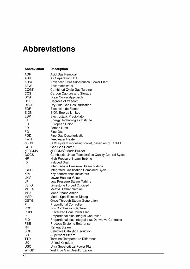
AGR Acid Gas RemovalASU Air Separation UnitAUSC Advanced Ultra Supercritical Power PlantBFW Boiler feedwaterCCGT Combined Cycle Gas TurbineCCS Carbon Capture and StorageDCA Drain Cooler ApproachDOF Degrees of freedomDFGD Dry Flue Gas DesulfurizationEDF Electricite de FranceE.ON E.ON Energy LimitedESP Electrostatic PrecipitatorETI Energy Technologies InstituteEU European UnionFD Forced DraftFG Flue GasFGD Flue Gas DesulfurizationFWH Feedwater HeatergCCS CCS system modelling toolkit, based on gPROMSGGH Gas-Gas HeatergPROMS gPROMS® ModelBuilderGQCS Combustion/Heat Transfer/Gas Quality Control SystemHP High Pressure Steam TurbineID Induced DraftIP Intermediate Pressure Steam TurbineIGCC Integrated Gasification Combined CycleKPI Key performance indicatorsLHV Lower Heating ValueLP Low Pressure Steam TurbineLSFO Limestone Forced OxidizedMDEA Methyl DiethanolamineMEA MonoEthanolAmineMSD Model Specification DialogOSTG Once-Through Steam GenerationP Proportional ControllerPCC Pos Combustion CapturePCPP Pulverized Coal Power PlantPI Proportional plus Integral ControllerPID Proportional plus Integral plus Derivative ControllerPSE Process Systems EnterpriseRH Reheat SteamSCR Selective Catalytic ReductionSH Superheat SteamTTD Terminal Temperature DifferenceUK United KingdomUSC Ultra Supercritical Power PlantWFGD Wet Flue Gas Desulfurization
xx
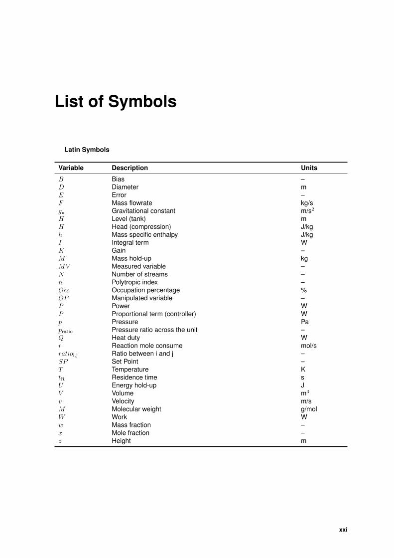
List of Symbols
Latin Symbols
Variable Description Units
B Bias –D Diameter mE Error –F Mass flowrate kg/sgn Gravitational constant m/s2
H Level (tank) mH Head (compression) J/kgh Mass specific enthalpy J/kgI Integral term WK Gain –M Mass hold-up kgMV Measured variable –N Number of streams –n Polytropic index –Occ Occupation percentage %OP Manipulated variable –P Power WP Proportional term (controller) Wp Pressure Papratio Pressure ratio across the unit –Q Heat duty Wr Reaction mole consume mol/sratioi,j Ratio between i and j –SP Set Point –T Temperature KtR Residence time sU Energy hold-up JV Volume m3
v Velocity m/sM Molecular weight g/molW Work Ww Mass fraction –x Mole fraction –z Height m
xxi
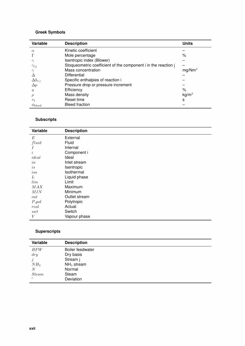
Greek Symbols
Variable Description Units
α Kinetic coefficient –Γ Mole percentage %γ Isentropic index (Blower) –γi,j Stoqueometric coefficient of the component i in the reaction j –γ Mass concentration mg/Nm3
∆ Differential –∆hr,i Specific enthalpies of reaction i –∆p Pressure drop or pressure increment –η Efficiency %ρ Mass density kg/m3
τI Reset time sφbleed Bleed fraction –
Subscripts
Variable Description
E Externalfluid FluidI Inlernali Component iideal Idealin Inlet streamis Isentropiciso IsothermalL Liquid phaselim LimitMAX MaximumMIN Minimumout Outlet streamP ,pol Polytropicreal Actualswt SwitchV Vapour phase
Superscripts
Variable Description
BFW Boiler feedwaterdry Dry basisj Stream jNH3 NH3 streamN NormalSteam Steam′ Deviation
xxii

1Introduction
Contents1.1 Motivation and Objectives . . . . . . . . . . . . . . . . . . . . . . . . . . . . . . . . 31.2 State of The Art . . . . . . . . . . . . . . . . . . . . . . . . . . . . . . . . . . . . . . 31.3 Original Contributions . . . . . . . . . . . . . . . . . . . . . . . . . . . . . . . . . . 41.4 Thesis Outline . . . . . . . . . . . . . . . . . . . . . . . . . . . . . . . . . . . . . . . 4
1
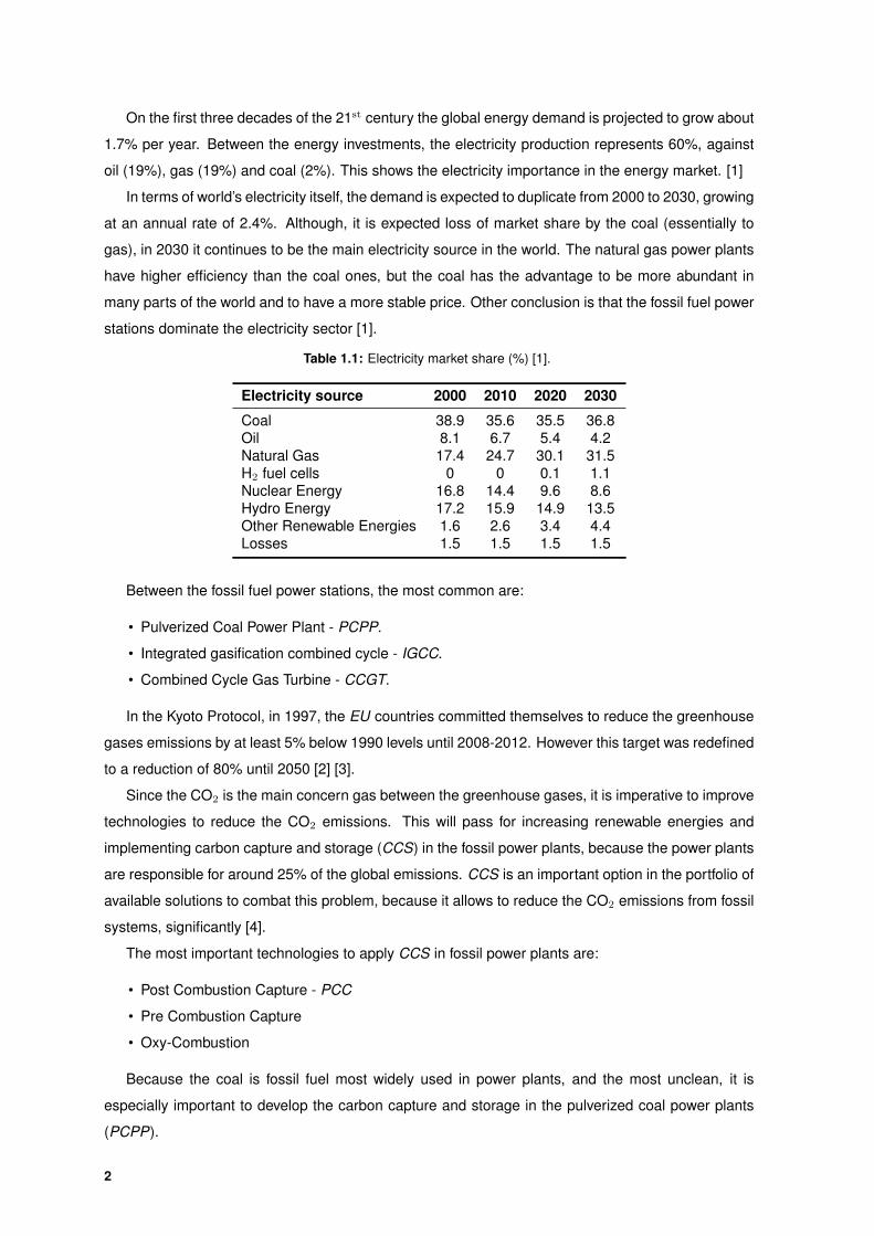
On the first three decades of the 21st century the global energy demand is projected to grow about
1.7% per year. Between the energy investments, the electricity production represents 60%, against
oil (19%), gas (19%) and coal (2%). This shows the electricity importance in the energy market. [1]
In terms of world’s electricity itself, the demand is expected to duplicate from 2000 to 2030, growing
at an annual rate of 2.4%. Although, it is expected loss of market share by the coal (essentially to
gas), in 2030 it continues to be the main electricity source in the world. The natural gas power plants
have higher efficiency than the coal ones, but the coal has the advantage to be more abundant in
many parts of the world and to have a more stable price. Other conclusion is that the fossil fuel power
stations dominate the electricity sector [1].
Table 1.1: Electricity market share (%) [1].
Electricity source 2000 2010 2020 2030
Coal 38.9 35.6 35.5 36.8Oil 8.1 6.7 5.4 4.2Natural Gas 17.4 24.7 30.1 31.5H2 fuel cells 0 0 0.1 1.1Nuclear Energy 16.8 14.4 9.6 8.6Hydro Energy 17.2 15.9 14.9 13.5Other Renewable Energies 1.6 2.6 3.4 4.4Losses 1.5 1.5 1.5 1.5
Between the fossil fuel power stations, the most common are:
• Pulverized Coal Power Plant - PCPP.
• Integrated gasification combined cycle - IGCC.
• Combined Cycle Gas Turbine - CCGT.
In the Kyoto Protocol, in 1997, the EU countries committed themselves to reduce the greenhouse
gases emissions by at least 5% below 1990 levels until 2008-2012. However this target was redefined
to a reduction of 80% until 2050 [2] [3].
Since the CO2 is the main concern gas between the greenhouse gases, it is imperative to improve
technologies to reduce the CO2 emissions. This will pass for increasing renewable energies and
implementing carbon capture and storage (CCS) in the fossil power plants, because the power plants
are responsible for around 25% of the global emissions. CCS is an important option in the portfolio of
available solutions to combat this problem, because it allows to reduce the CO2 emissions from fossil
systems, significantly [4].
The most important technologies to apply CCS in fossil power plants are:
• Post Combustion Capture - PCC
• Pre Combustion Capture
• Oxy-Combustion
Because the coal is fossil fuel most widely used in power plants, and the most unclean, it is
especially important to develop the carbon capture and storage in the pulverized coal power plants
(PCPP).
2
Although the CCS reduces the efficiency in the energy production in the power plants, investments
must be done in this area to improve the technologies and achieve the CCS objective without com-
promising the electricity sector. At the current state of technology, units retrofitted with carbon capture
would suffer a decrease around 12% in the efficiency and an increase between 20 and 30% in the
coal consume to supply the same electricity output [5] [6].
Due to this panorama, in September 2011, ETI (Energy Technologies Institute), responsible for
projects to improve the energy sector, founded the CCS project to study this problem and to accelerate
the carbon capture and storage in UK, a technology that will become increasingly important because
the emissions capital penalty will reach the CCS investment and efficiency penalty in applying capture.
1.1 Motivation and Objectives
PSE integrated the ETI-CCS project in September 2011 with the objective to build the gCCS toolkit
in collaboration with important “stakeholders” in this area, such as E.ON, EDF and Rolls Royce. This
tool incorporates the modelling in gPROMS of power generation and CO2 capture, compression,
transmission, injection and storage.
The final tool will be important to study this new theme. For example, it will allow to design, to
simulate, to control and to optimize the full chain. The models’ flexibility and robustness is really
important to let the all chain respond to different consumers’ demands as quick as possible.
Since the gCCS project is in the pulverized coal power plant (PCPP) modelling phase, this thesis
is incorporated in the construction of a pulverized coal power plant modelling kit, the most problematic
power plant in terms of CO2 emissions.
The thesis objective is to design a power plant with operational data and to simulate the operation
of the designed power plant, with control incorporated. It is used operational data from a subcritical
PCPP ’s steam cycle ([7]), it is implemented one of the different types of control (boiler following
control) and the simulations consist in set point changes (daily cycle, e.g.) and disturbances to the
system.
To do the final flowsheet several gCCS models are required. Some of the models that need to be
developed to the gCCS library are done in the scope of the thesis: Deaerator, SCR, Blower, Controller
and Drum.
1.2 State of The Art
A lot of work has been developed in the scope of power plant modelling.
Lots of reports focused in performance studies to the different kinds of power plants have been
done. In these studies the performance of power plants when connected to the several CCS tech-
nologies is commonly analysed , both for retrofit and for newly built.
An example of this kind of study applied to a PCPP is a report done by the US Department
of Energy. Using test data, it was developed a steady-state model for the boiler of an existing power
3
plant, and it was used to study the base case (power plant without capture) and three capture concepts
[8].
Also developed by the US Department of Energy and inserted in the problem of CO2 capture, is
the study of cost and performance of a power plant with and without capture, using for it the ASPEN
Plus modelling program. For example, PCPP with different technologies and conditions were target
of this study [9].
In terms of power plant control modelling one interesting work was developed is the University
of Rostock. The dynamic model was focused on the water/steam circuit, the combustion chamber
and the coal mills. It’s based on a real 550 MW power plant (Rostock), and it was develop using a
non-commercial Modelica library ThermoPower [10].
Another case found is the ”modelling and control of a supercritical coal fired boiler”, where it is
applied the coordinated control system to control the steam generation’s system [11].
By way of conclusion, the power plants have been the target of several modeling projects and the
most recent developments have been in the framework of CCS. The gross of the models done for
power plants are linked to the study of performances, but there is also some work done in dynamic
modelling with control to simulate shut-down, start-up and load changes.
1.3 Original Contributions
The thesis presents the modelling of a pulverized coal power plant and some of its units, using the
gPROMS as modelling program, a work never done before in this software. Besides that, the thesis
is inserted in an innovative project in the framework of CCS.
It was modeled some models that compose the power plant, which were connected together to
represent the real power plant. The main objective of this thesis is to simulate dynamic control and to
study the performance at different operational conditions (different loads, e.g.), something never done
before nor in the scope of the ETI-CCS project nor in gPROMS.
1.4 Thesis Outline
This thesis is organised in the following way.
It is presented, in the Chapter 2, the background on the subject, describing the pulverized coal
power plant and its equipments, as well as its control system. It was also done a brief description of
the CCS technologies. The next Chapter (3) consists in the mathematical description of the several
developed component models. In the chapter 4 is presented the main objective of the thesis. Here are
explained the flowsheet models for design, operational and control modes and submitted the results.
To finish this chapter it’s done some sensitivity analyses to the system. The conclusions and future
work are summarized in the 5.
4

2Background
Contents2.1 Pulverized Coal Power Plant . . . . . . . . . . . . . . . . . . . . . . . . . . . . . . . 62.2 Pulverized Coal Power Plant Control . . . . . . . . . . . . . . . . . . . . . . . . . . 212.3 Carbon Capture and Storage . . . . . . . . . . . . . . . . . . . . . . . . . . . . . . . 26
5
2.1 Pulverized Coal Power Plant
Pulverized Coal Power Plant is a thermal power plant that uses the chemical energy of the coal to
produce electric energy. It starts by converting the chemical energy of the coal (heat of combustion)
into thermal energy (steam), then converts the thermal energy into mechanical energy (turbines’
rotation) and finishes producing electric energy in the generator using the mechanical energy [12].
The Pulverized Coal Power Plant is one of the most used methods to produce energy, and has the
following advantages [12]:
• High efficiency (table 2.1)
• Lower capital cost
• Adaptability to burn every types of coal
• Technologies to clean the flues gas are established
• Low consume of water (closed cycle minimizes the mass lost)
• Easy and reliable access to coal in many parts of the world
Energy efficiency (same as “net” efficiency) of a power plant is the useful work output over the heat
input. The heat input is the coal chemical heat and the useful work is the electrical power produced,
deducting the electrical power used (e.g., pumps and refrigerating tower). The thermal (or “gross”)
efficiency does not take into account the power spent for own use [6].
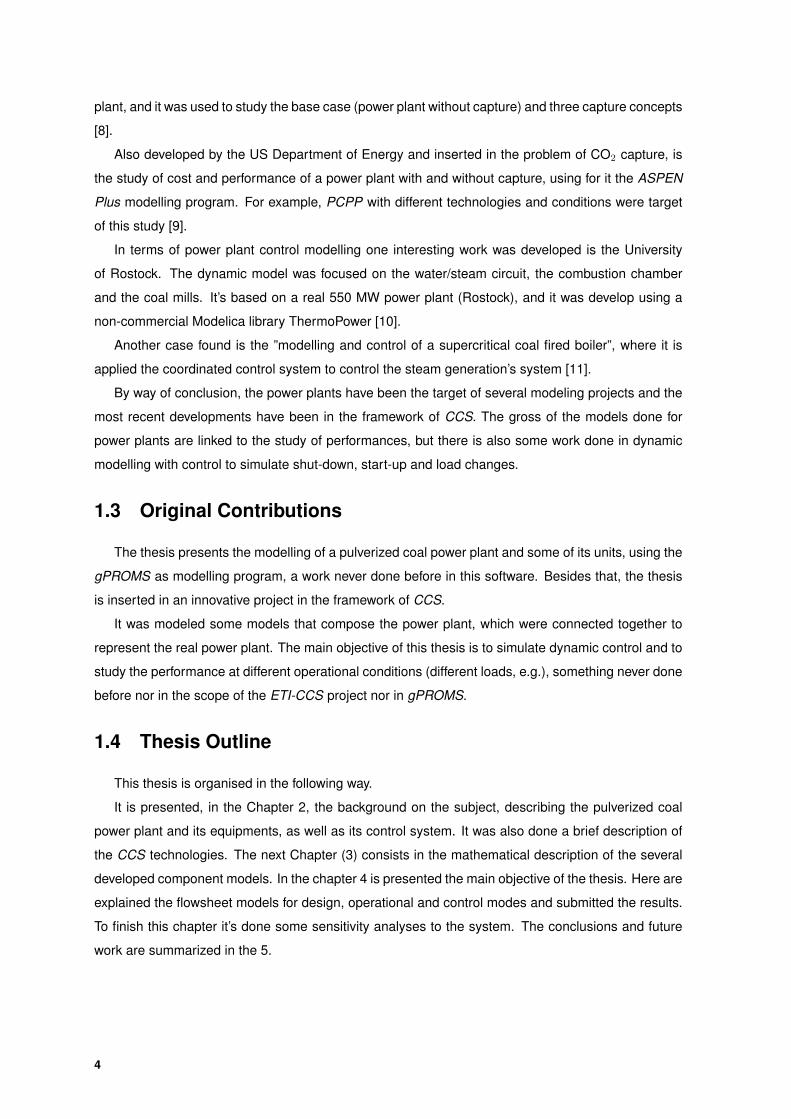
This type of power plant must have the following units (figure 2.1):
Figure 2.1: Pulverized Coal Power Plant blocs diagram [12].
Regarding the current technologies, the power plant can be subcritical, supercritical, advanced
supercritical or ultra supercritical. In the first case the steam conditions are bellow the critical point
(374°C and 220bar), while on the other three types of power plants the steam is above those condi-
tions. On the following table (2.1), it is presented the typical steam conditions, efficiencies and CO2
emissions for the four cases:
6
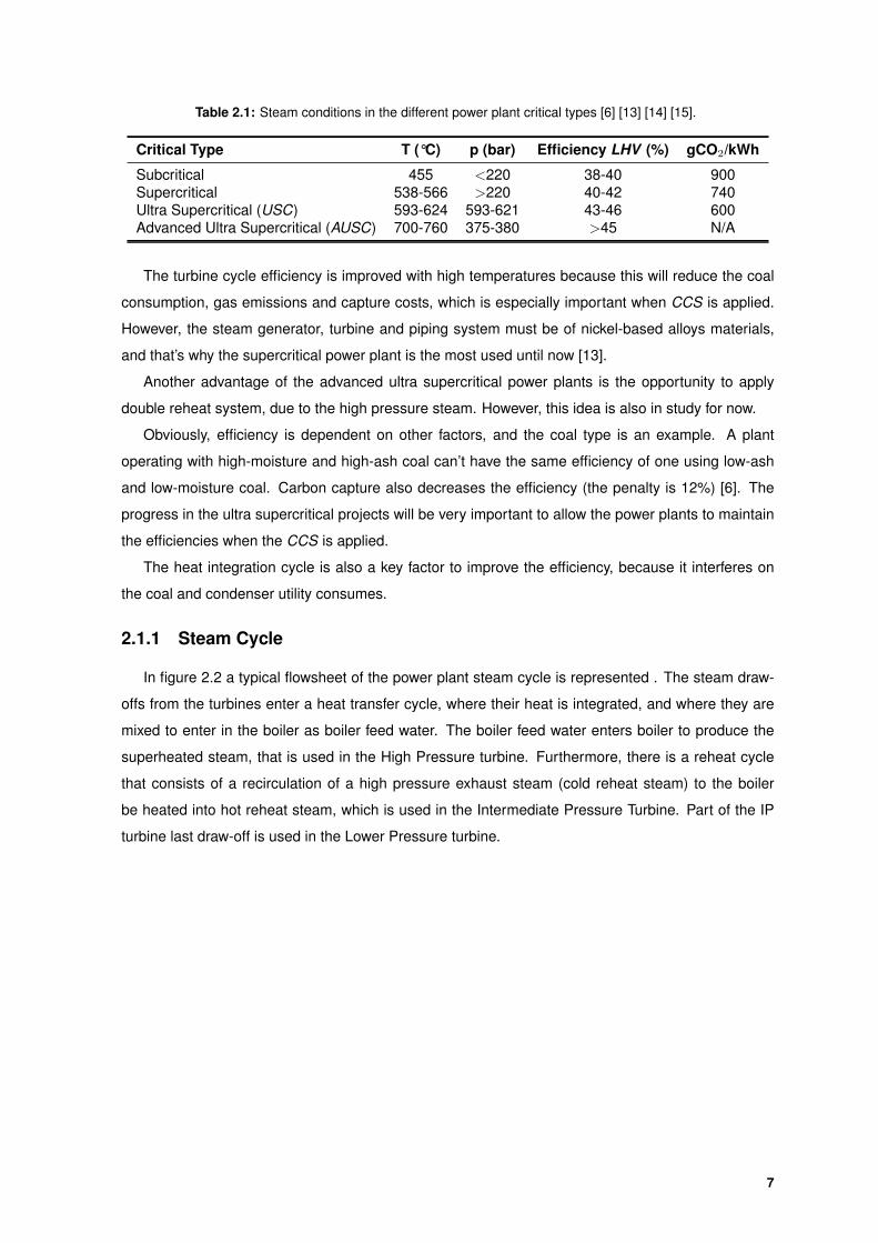
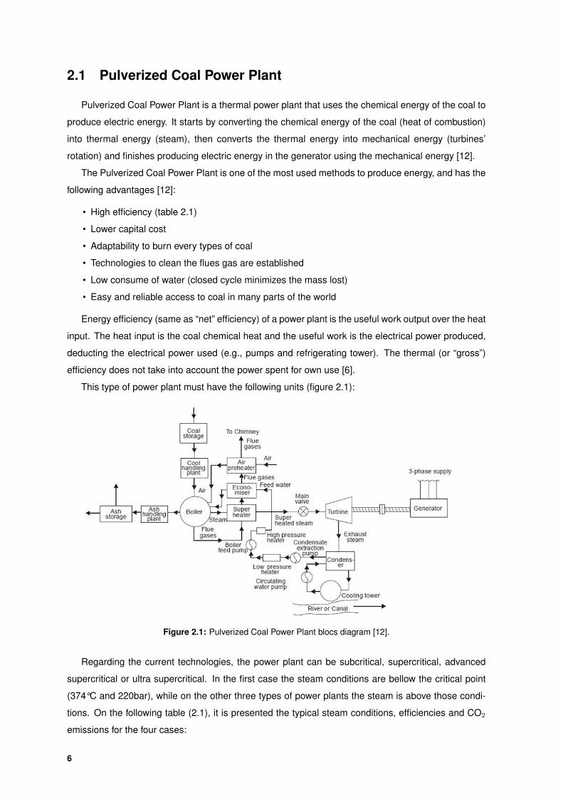
Table 2.1: Steam conditions in the different power plant critical types [6] [13] [14] [15].
Critical Type T (°C) p (bar) Efficiency LHV (%) gCO2/kWh
Subcritical 455 <220 38-40 900Supercritical 538-566 >220 40-42 740Ultra Supercritical (USC) 593-624 593-621 43-46 600Advanced Ultra Supercritical (AUSC) 700-760 375-380 >45 N/A
The turbine cycle efficiency is improved with high temperatures because this will reduce the coal
consumption, gas emissions and capture costs, which is especially important when CCS is applied.
However, the steam generator, turbine and piping system must be of nickel-based alloys materials,
and that’s why the supercritical power plant is the most used until now [13].
Another advantage of the advanced ultra supercritical power plants is the opportunity to apply
double reheat system, due to the high pressure steam. However, this idea is also in study for now.
Obviously, efficiency is dependent on other factors, and the coal type is an example. A plant
operating with high-moisture and high-ash coal can’t have the same efficiency of one using low-ash
and low-moisture coal. Carbon capture also decreases the efficiency (the penalty is 12%) [6]. The
progress in the ultra supercritical projects will be very important to allow the power plants to maintain
the efficiencies when the CCS is applied.
The heat integration cycle is also a key factor to improve the efficiency, because it interferes on
the coal and condenser utility consumes.
2.1.1 Steam Cycle
In figure 2.2 a typical flowsheet of the power plant steam cycle is represented . The steam draw-
offs from the turbines enter a heat transfer cycle, where their heat is integrated, and where they are
mixed to enter in the boiler as boiler feed water. The boiler feed water enters boiler to produce the
superheated steam, that is used in the High Pressure turbine. Furthermore, there is a reheat cycle
that consists of a recirculation of a high pressure exhaust steam (cold reheat steam) to the boiler
be heated into hot reheat steam, which is used in the Intermediate Pressure Turbine. Part of the IP
turbine last draw-off is used in the Lower Pressure turbine.
7
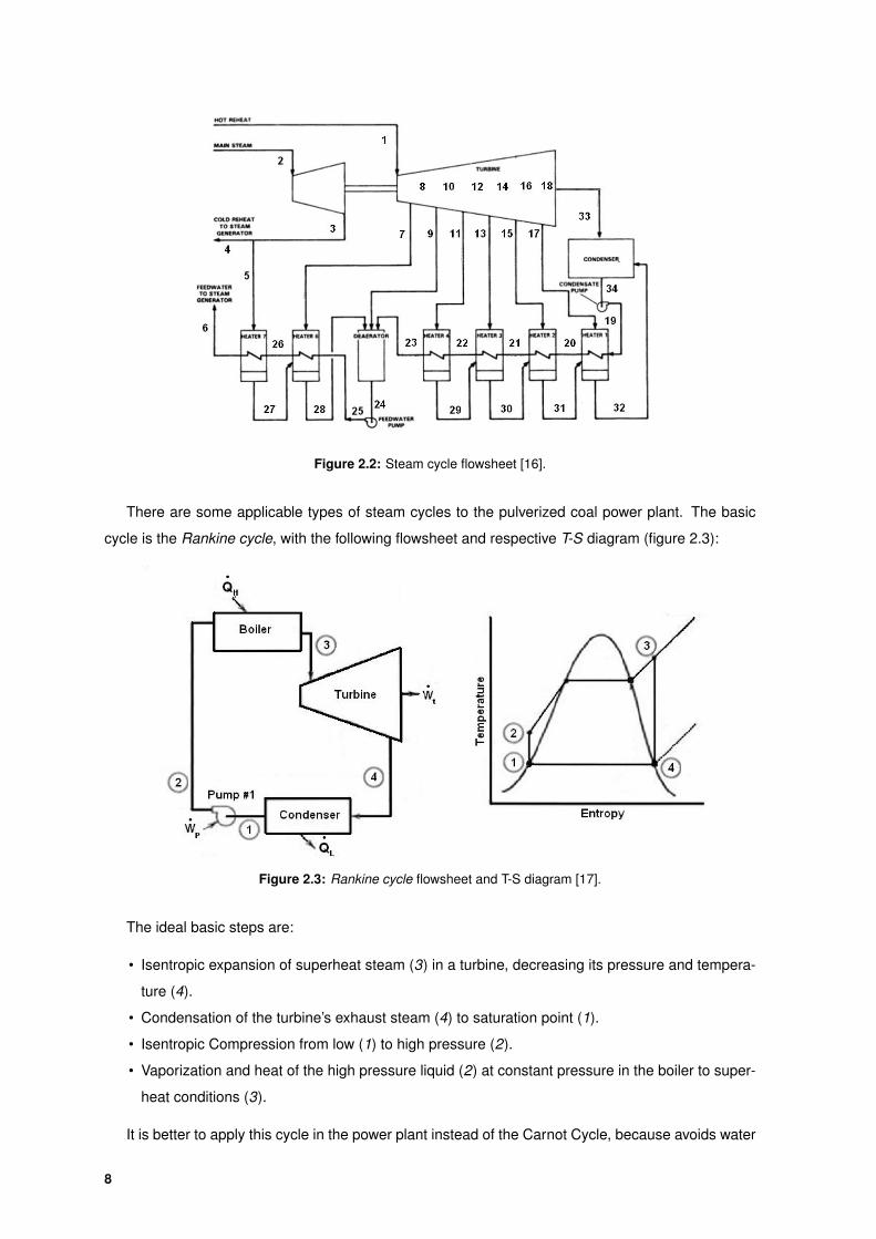
Figure 2.2: Steam cycle flowsheet [16].
There are some applicable types of steam cycles to the pulverized coal power plant. The basic
cycle is the Rankine cycle, with the following flowsheet and respective T-S diagram (figure 2.3):
Figure 2.3: Rankine cycle flowsheet and T-S diagram [17].
The ideal basic steps are:
• Isentropic expansion of superheat steam (3) in a turbine, decreasing its pressure and tempera-
ture (4).
• Condensation of the turbine’s exhaust steam (4) to saturation point (1).
• Isentropic Compression from low (1) to high pressure (2).
• Vaporization and heat of the high pressure liquid (2) at constant pressure in the boiler to super-
heat conditions (3).
It is better to apply this cycle in the power plant instead of the Carnot Cycle, because avoids water
8
in the pump and in the turbines (1 and 4).
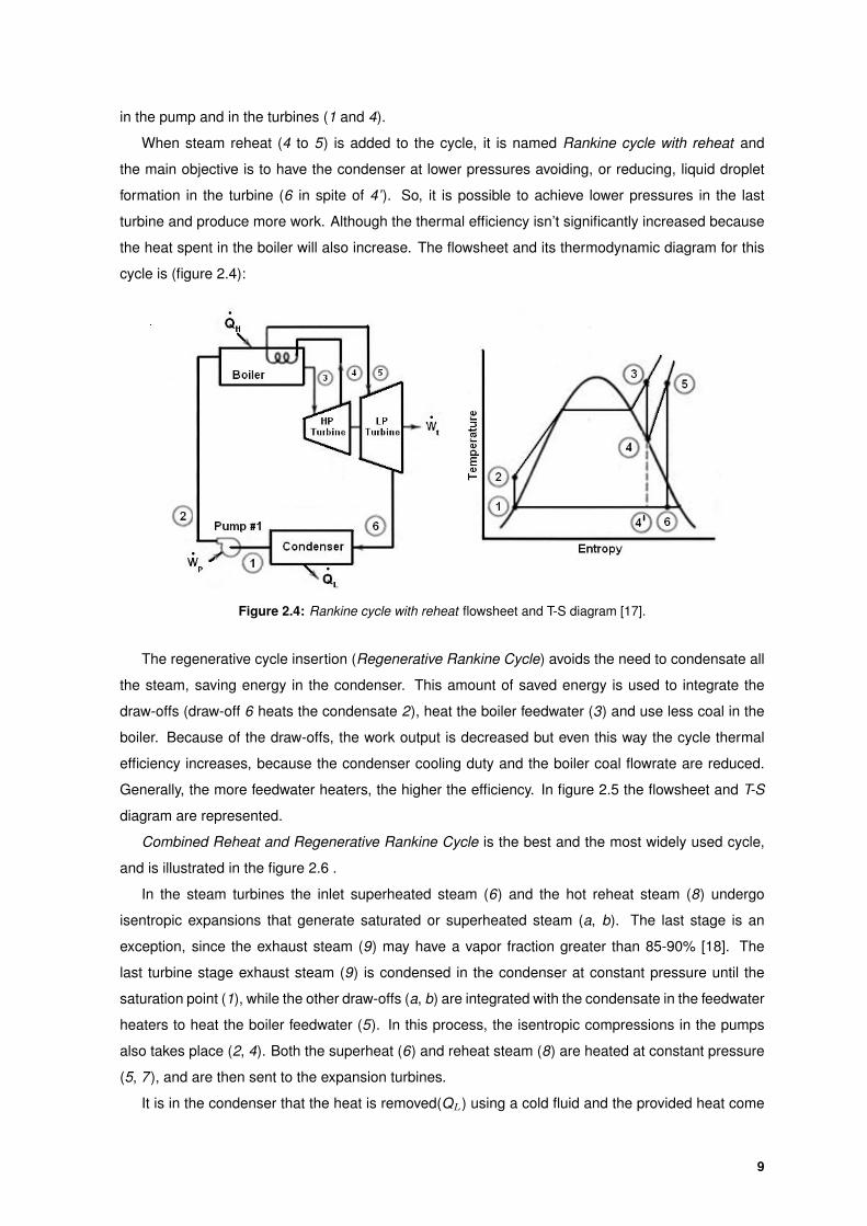
When steam reheat (4 to 5) is added to the cycle, it is named Rankine cycle with reheat and
the main objective is to have the condenser at lower pressures avoiding, or reducing, liquid droplet
formation in the turbine (6 in spite of 4’). So, it is possible to achieve lower pressures in the last
turbine and produce more work. Although the thermal efficiency isn’t significantly increased because
the heat spent in the boiler will also increase. The flowsheet and its thermodynamic diagram for this
cycle is (figure 2.4):
Figure 2.4: Rankine cycle with reheat flowsheet and T-S diagram [17].
The regenerative cycle insertion (Regenerative Rankine Cycle) avoids the need to condensate all
the steam, saving energy in the condenser. This amount of saved energy is used to integrate the
draw-offs (draw-off 6 heats the condensate 2), heat the boiler feedwater (3) and use less coal in the
boiler. Because of the draw-offs, the work output is decreased but even this way the cycle thermal
efficiency increases, because the condenser cooling duty and the boiler coal flowrate are reduced.
Generally, the more feedwater heaters, the higher the efficiency. In figure 2.5 the flowsheet and T-S
diagram are represented.
Combined Reheat and Regenerative Rankine Cycle is the best and the most widely used cycle,
and is illustrated in the figure 2.6 .
In the steam turbines the inlet superheated steam (6) and the hot reheat steam (8) undergo
isentropic expansions that generate saturated or superheated steam (a, b). The last stage is an
exception, since the exhaust steam (9) may have a vapor fraction greater than 85-90% [18]. The
last turbine stage exhaust steam (9) is condensed in the condenser at constant pressure until the
saturation point (1), while the other draw-offs (a, b) are integrated with the condensate in the feedwater
heaters to heat the boiler feedwater (5). In this process, the isentropic compressions in the pumps
also takes place (2, 4). Both the superheat (6) and reheat steam (8) are heated at constant pressure
(5, 7 ), and are then sent to the expansion turbines.
It is in the condenser that the heat is removed(QL) using a cold fluid and the provided heat come
9
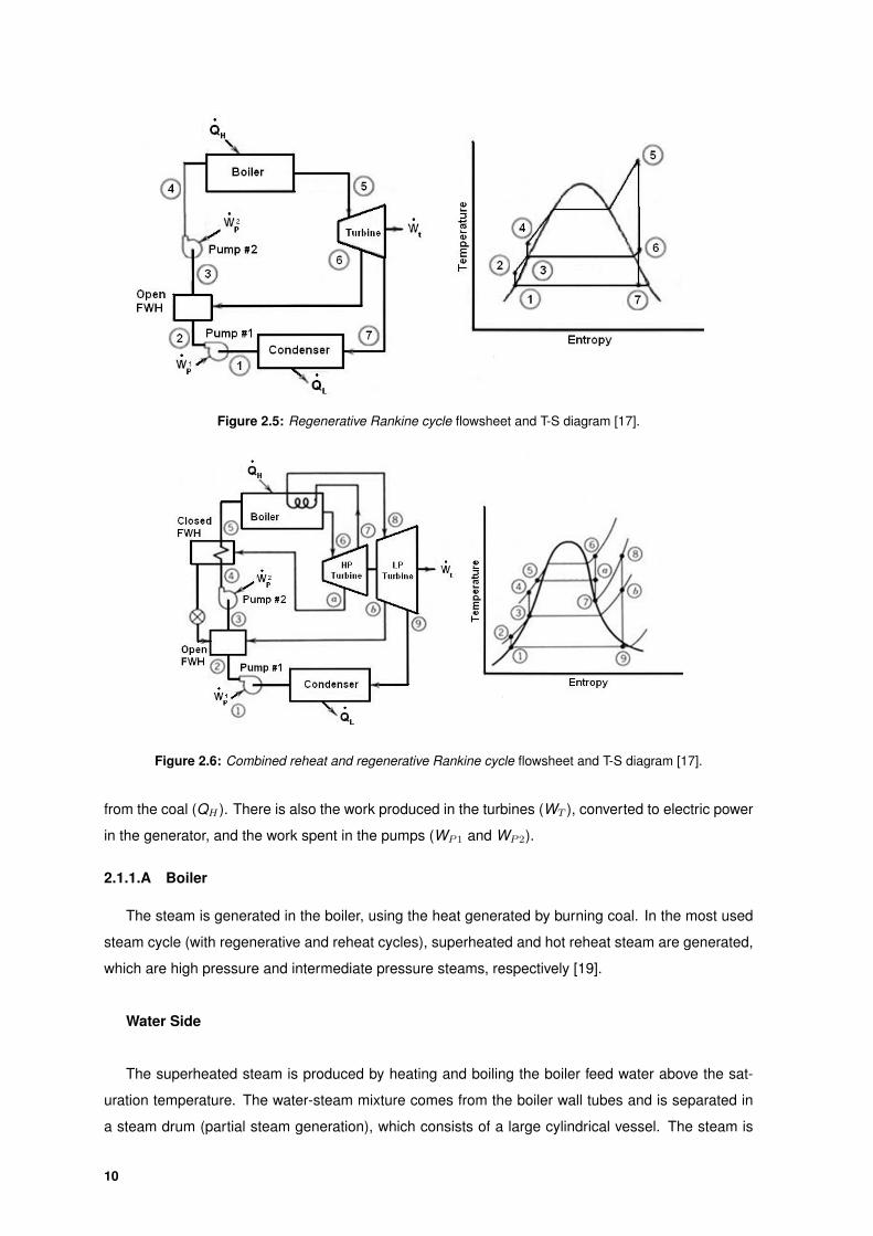
Figure 2.5: Regenerative Rankine cycle flowsheet and T-S diagram [17].
Figure 2.6: Combined reheat and regenerative Rankine cycle flowsheet and T-S diagram [17].
from the coal (QH ). There is also the work produced in the turbines (WT ), converted to electric power
in the generator, and the work spent in the pumps (WP1 and WP2).
2.1.1.A Boiler
The steam is generated in the boiler, using the heat generated by burning coal. In the most used
steam cycle (with regenerative and reheat cycles), superheated and hot reheat steam are generated,
which are high pressure and intermediate pressure steams, respectively [19].
Water Side
The superheated steam is produced by heating and boiling the boiler feed water above the sat-
uration temperature. The water-steam mixture comes from the boiler wall tubes and is separated in
a steam drum (partial steam generation), which consists of a large cylindrical vessel. The steam is
10
then heated in the superheater(s), and the water recirculates to the boiler tubes by natural or forced
circulation. The wall tubes increase the transfer heat and help to avoid the furnace material to high
temperatures.
In spite of a steam drum, the OTSG system can be used (”once-through steam generation”), which
has a coordinated control of the water flow and of heat input to assure that no water leaves with the
steam.
Futhermore, the boiler includes an economizer that pre-heats the boiler feed water, before entering
the boiler wall tubes, using waste heat that remained in the flue gas. This flue gas is typically between
180 and 260°C, and most of the economizers are able to raise the feedwater temperature from 11
to 17°C. The flue gas cooling is limited by the dew point, around 163°C, to avoid condensation and
formation of corrosive acids (mainly carbonic acid and sulfuric acid) [20].
The hot reheat steam is obtained by heating the cold reheat steam in the reheater. The super-
heaters and reheater consist of bundles of tubes, with steam passing inside the tubes and flue gas
passing outside, and the heat is transferred by convection.
Flue Gas Side
The boiler heat comes from the combustion of pulverized coal with air, in the furnace. In the
furnace, the flue gas evaporates the feedwater in the wall tubes, and then it passes to the convec-
tion zone, where the flue gas contacts with the superheaters, the reheater and the economizer heat
surfaces. When it leaves the boiler, it passes through the air pre-heater.
An important variable is the coal’s LHV (Lower Heating Value), that measures its specific combus-
tion energy.
In the furnace, pre-heated hot air and burners are used to burn the pulverized coal. The air is
classified as primary or secondary air. The primary air is 20-30% of the total air, and is used to dry
and pneumatically transport the coal to the burners, while the remaining air (secondary air) is directly
mixed in the burners with the coal/primary air mixture. To burn pulverized coal the type of furnace
used is a chamber fired furnace and the type of burners are chosen according to the conditions [12].
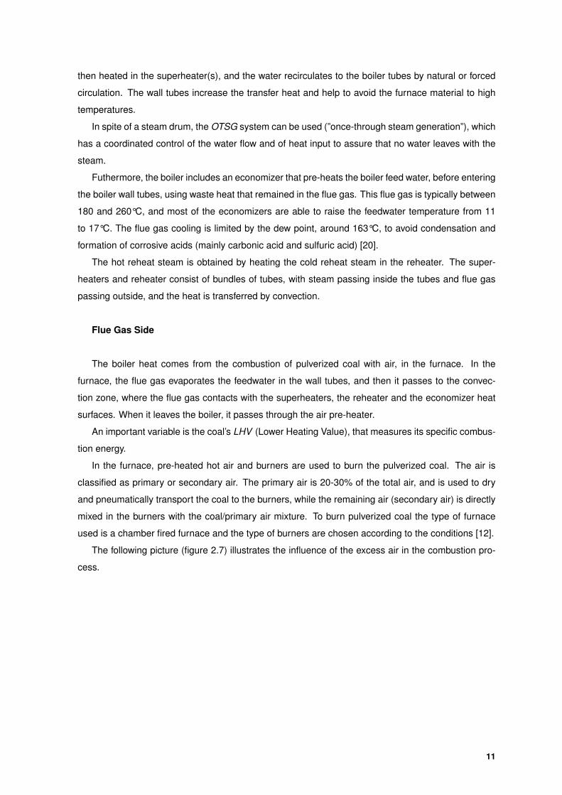
The following picture (figure 2.7) illustrates the influence of the excess air in the combustion pro-
cess.
11
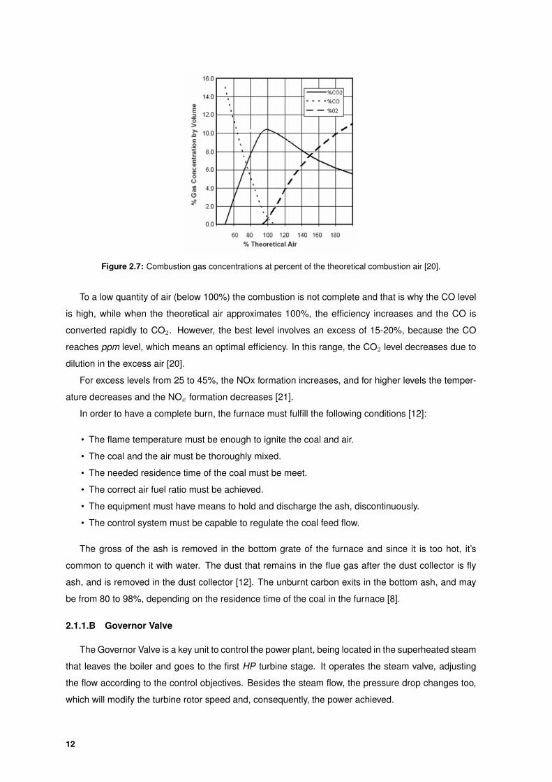
Figure 2.7: Combustion gas concentrations at percent of the theoretical combustion air [20].
To a low quantity of air (below 100%) the combustion is not complete and that is why the CO level
is high, while when the theoretical air approximates 100%, the efficiency increases and the CO is
converted rapidly to CO2. However, the best level involves an excess of 15-20%, because the CO
reaches ppm level, which means an optimal efficiency. In this range, the CO2 level decreases due to
dilution in the excess air [20].
For excess levels from 25 to 45%, the NOx formation increases, and for higher levels the temper-
ature decreases and the NOx formation decreases [21].
In order to have a complete burn, the furnace must fulfill the following conditions [12]:
• The flame temperature must be enough to ignite the coal and air.
• The coal and the air must be thoroughly mixed.
• The needed residence time of the coal must be meet.
• The correct air fuel ratio must be achieved.
• The equipment must have means to hold and discharge the ash, discontinuously.
• The control system must be capable to regulate the coal feed flow.
The gross of the ash is removed in the bottom grate of the furnace and since it is too hot, it’s
common to quench it with water. The dust that remains in the flue gas after the dust collector is fly
ash, and is removed in the dust collector [12]. The unburnt carbon exits in the bottom ash, and may
be from 80 to 98%, depending on the residence time of the coal in the furnace [8].
2.1.1.B Governor Valve
The Governor Valve is a key unit to control the power plant, being located in the superheated steam
that leaves the boiler and goes to the first HP turbine stage. It operates the steam valve, adjusting
the flow according to the control objectives. Besides the steam flow, the pressure drop changes too,
which will modify the turbine rotor speed and, consequently, the power achieved.
12
This operation is a throttling process, since there occurs a pressure drop, the temperature de-
creases, but no energy change occurs (isenthalpic) [22].
2.1.1.C Steam Turbine
The steam turbine is an important equipment because it produces the mechanical energy.
There is usually a high pressure (HP), an intermediate pressure (IP) and a low pressure (LP)
steam turbine, each one with varied number of extraction points. The extraction points location is a
function of the power plant optimization, since it will change the work produced and the integrated
heat in the heat integration zone.
The force applied in the turbine is proportional to the change of the momentum, so the principle
of the turbine is to use the high velocity of the jet steam to impact the turbine’s curve blades and to
move them. The steam enters the turbine through a nozzle, where the pressure falls and is converted
into kinetic energy, resulting in a high velocity jet [12].
The turbine is designed to maintain the steam velocity and not to produce power, if the blade is
locked. On the other hand, if the blade is allowed to speed up the power increases and the outlet
velocity decreases due to the momentum change that caused the force. The power reaches the
maximum when the blade velocity is 50% of the steam velocity, at which the outlet velocity is near
zero. The turbine includes a row of nozzles, a row of moving blades and the casing (cylinder).
Nowadays, on the PCPP it’s always used single pressure and reheat turbines. The single pressure
is the most common (there is a single source of steam supply), and the reheat is used in the reheat
cycle (the steam is taken from, reheated and returned to the turbine). In terms of heat rejection,
regenerative and condensing turbines are used, the first to send draw-offs to the heat transfer cycle
and the second to be used on the last stage. The condensing turbine has its exhaust pressure fixed
by the condenser.
If there is a capture plant, intermediate pressure draw-off is usually sent to its reclaimer.
In an isentropic expansion there aren’t energy losses due to friction or other thermodynamic
losses, which means that the steam entropy doesn’t change. This is a good assumption to calcu-
late the ideal power (equation 2.1) [22]:
Wis = F (hin − his,out) (2.1)
To calculate the actual power, it’s used the isentropic efficiency, which relates the actual work with
the work obtained in the ideal case (equation 2.2)[22]:
ηis =Wreal
Wis=
hin − hout
hin − his,out(2.2)
2.1.1.D Generator
The generator is directly coupled to the steam turbine and converts the turbines’ rotating mechani-
cal power into electrical power to supply to the grid. The generator rotor is magnetized and its rotation
generates the electrical power in the generator stator.
13
2.1.1.E Heat Transfer Cycle
The heat transfer cycle has the simplified objective of mixing all the turbine steam draw-offs, in-
tegrating their heat, and sending the material to the boiler as boiler feed water. It’s also named the
regenerative cycle, and it was described in section 2.1.1 [23].
”Condensate” is the water leaving the condenser and passing through the low pressure feedwa-
ter heaters, while the water leaving the deaerator and passing through the high pressure feedwater
heaters is called ”boiler feedwater”. In most of the modern heat cycles there are feedwater heaters, a
condenser and a deaerator, which use extracted steam from the steam turbine.
The turbines’ draw-offs have different temperatures and pressures, due to the different outlet pres-
sure in each turbine stage. Because of this the draw-offs are used to heat the feedwater in different
feedwater heaters.
After the integration in the low pressure feedwater heaters line, the condensates are mixed in the
deaerator. The deaerator’s outlet is sent to the boiler, after being heated in the high pressure feedwa-
ter heaters line.
Condenser
The condenser is the single unit inside the heat integration cycle responsible of removing heat by
an external utility. The amount of heat duty is crucial to the power plant operation to allow the heat
integration and the draw-offs condensation in the consequents feedwater heaters, and that’s why the
saturated condensate pressure must be very low. The fact that the work output in the turbines and,
consequently, the power plant efficiency, increase with lower exhaust temperatures is also a reason
to lower the condenser pressure [12] [23] [24].
Usually the condensation heat removal is done using cooling water, and only in few occasions,
when water isn’t available, air is used as a cooler. If water is used it’s advantageous to have a cooling
water closed cycle to control water quality.
The most common condenser type is a tube and shell heat exchanger, with the water passing
through the tubes and the steam through the shell from the top downward, which is characterized
as a surface condenser. Some of the advantages of this type of condenser are the possibility to use
impure water because it doesn’t contact the condensate, to use to condensate as boiler feedwater and
to do high vacuum. Although it requires more space, the capital cost is larger and the maintenance
and running cost is high.
Another type of condenser is the jet condenser, which mixes directly the steam and the cooling
water.
Feedwater Heater
The number of feedwater heaters depends mainly on the size of the turbines, on the inlet and
exhaust steam conditions, on the overall plant size and on the economic considerations. Because the
number of feedwater heaters influences the heat integration, it plays a key role and must be part of
the design to optimize the plant efficiency [23].
14
The feedwater heater must have water passing through the cold side (tubes) and draw-off steam
passing for the hot side (shell), in counter current. Besides that, it can have one inlet as drains, which
is the draw-off steam condensate from other feedwater heater (with higher pressure steam). In this
case, the drain and the draw-off steam are mixed in the hot side, and the drain is vaporized due to the
pressure decrease.
In the feedwater heater the steam condensates in its chamber and the cold steam passes through
the tubes. Along the unit there are three main zones [25]:
• Desuperheating: cooling of the superheated steam to the saturation point.
• Condensing: energy from the steam/water mixture condensation is used to preheat the boiler
feedwater.
• Sub-cooling: used to capture additional energy from the liquid.
It is possible to exchange the heat mixing all the streams (”open” FWH). However, it’s not advan-
tageous because it will require another pump in the outlet.
In the shell side it must be maintained a liquid level that optimizes the heat transfer from the steam
to the boiler feedwater.
The performance of the feedwater heater can be evaluated measuring the feedwater temperature
rise, the terminal temperature difference (TTD) or the drain cooler approach (DCA). The first one is
the temperature increase in the cold side, while the second one is difference between the draw-off
steam saturation temperature and the cold side outlet temperature. DCA is the difference between
the drains and the inlet cold side temperatures.
Deaerator
The main Deaerator’s objective is to remove dissolved gases from the water, to avoid the ac-
cumulation due to gas leakage into the system. That’s important because, for example, the excess
oxygen and carbon dioxide increases the metal corrosion. To prevent corrosion (carbonic acid) volatile
neutralizing amines are usually used to adjust the pH. In order to remove oxygen sodium sulfite, Hy-
droquinone Hydrazine, Diethylhydroxyamine and/or Methyl ethyl ketoxime are used [20] [23] [24] [26]
[27].
Besides the gas removal, it’s also usual to remove the hard salts here. The hard salts deposit in the
surfaces (”scale”) and decrease the heat transfer quality in the heat exchangers, preventing and ad-
equate flow the tubes and forcing blowdown in the boiler. Calcium and magnesium bicarbonate form
an alkaline solution (”alkaline” hardness), and are easily removed by boiling (”temporary” hardness).
The most problematic are the calcium and magnesium sulfates, chlorides and nitrates (”non alkaline”
hardness) that must be removed with reagents (Polyphosphates and Sodium Meta Phosphate).
The secondary purposes of this unit are to accumulate water to feed the boiler (usually 5 minutes
of feedwater content), and to provide proper suction conditions for the boiler feed pump. It receives
the condensates to be treated, that come from the condenser and/or feedwater heaters, and a steam
stream (turbine or boiler draw-off). The deaerator is composed by three sections: the heat section,
15
the vent condenser and the storage section.
The gases are removed by two mechanisms that occur in the heating section.
• On the first one, the water is heated in the heater section, in direct contact with the steam. This
decreases gases solubility in water due to reduction of gas partial pressure in the gas phase;
• On the second mechanism, the water enters the deaerator head through a nozzle (spray type
deaerator) and contacts with the rising steam to increase the mass and heat transfer rate, in
order to remove the gases from the water to the steam, to achieve the saturation point and to
condensate the majority of the steam. The same principle can be achieved passing the water
through a set of layers in counter current with the steam (layer type deaerator).
In the vent condenser the incoming condensates pass through the tubes of a heat exchanger
mounted on the top of the deaerator to condensate part of the steam that escaped through the vent.
The heated and deaerated condensate, along with the condensate steam, falls to the storage section
located below the deaerator. This last section has the purpose of accumulating feedwater.
The steam that escapes with the gases is compensated with make-up water, which has to be ex-
ternally treated.
Pump
The pump is used to transport the water in the heat cycle. Usually it’s only needed one pump to
pump the condensate and another to pump to the feedwater, through the FWH tubes. This is not true
if there is any ”open” feedwater heater which requires a pump on its outlet.
Pumps increase the velocity, the pressure, the mechanical energy, or all of them. The most used
pumps are positive-displacement and centrifugal pumps. The first applies pressure by a reciprocating
piston or rotating member in a chamber, which is alternately filled and emptied of liquid. The centrifu-
gal one uses rotational high velocities and convert the kinetic energy into pressure energy. The work
delivered to the fluid is calculated from the mass flowrate and the head development (equation 2.3)
[28]:
Wfluid = F∆Hp (2.3)
Power supplied to the pump is calculated with the efficiency (equation 2.4) [28]:
Wreal =Wfluid
η(2.4)
The head comes from the Bernoulli equation and is(equation 2.5) [28]:
Hp =p
ρ+ gnz + α
v2
2(2.5)
The pumps represent a large fraction of the auxiliary power consumed in the plant, since their
flows are very big and the boiler feedwater pump pressure increase is from low to high pressures.
Water make-up [20]
Although the steam cycle is a closed cycle, there are material losses due to, for example:
16
• Boiler blowdown
• Deaerator steam vent losses
• Unreturned condensate (lost in the vacuum system)
• Leakage
Because of these losses a water make-up is performed in the condenser tank. This make-up water
must be chemically treated.
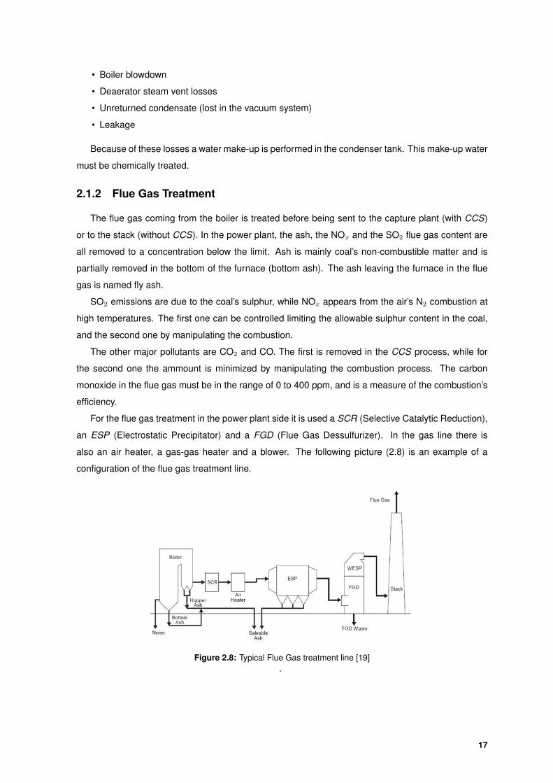
2.1.2 Flue Gas Treatment
The flue gas coming from the boiler is treated before being sent to the capture plant (with CCS)
or to the stack (without CCS). In the power plant, the ash, the NOx and the SO2 flue gas content are
all removed to a concentration below the limit. Ash is mainly coal’s non-combustible matter and is
partially removed in the bottom of the furnace (bottom ash). The ash leaving the furnace in the flue
gas is named fly ash.
SO2 emissions are due to the coal’s sulphur, while NOx appears from the air’s N2 combustion at
high temperatures. The first one can be controlled limiting the allowable sulphur content in the coal,
and the second one by manipulating the combustion.
The other major pollutants are CO2 and CO. The first is removed in the CCS process, while for
the second one the ammount is minimized by manipulating the combustion process. The carbon
monoxide in the flue gas must be in the range of 0 to 400 ppm, and is a measure of the combustion’s
efficiency.
For the flue gas treatment in the power plant side it is used a SCR (Selective Catalytic Reduction),
an ESP (Electrostatic Precipitator) and a FGD (Flue Gas Dessulfurizer). In the gas line there is
also an air heater, a gas-gas heater and a blower. The following picture (2.8) is an example of a
configuration of the flue gas treatment line.
Figure 2.8: Typical Flue Gas treatment line [19].
17
2.1.2.A Electrostatic precipitator
The flue gas that comes from the furnace has particulate matter that has as majority compo-
nent fly ash, which must be collected. To this end, a Electrostatic Precipitator (ESP), Fabric Filters
(Baghouses), mechanical collectors and venture scrubbers are employed. The most used is the dry
electrostatic precipitator [19].
Dry Electrostatic Precipitator
The ESP creates an electric field (between CEs - positive polarity - and DEs - negative polarity)
where the flue gas passes, and the particulates are electrically charged. The negatively charged ash
particles migrate toward the CEs. Depending on the particles size, the electrification may be easy to
perform and the flue gas velocity is a key factor to the particles have enough residence time to be
charged and collected. Plates are installed to collect the ash layer, and this particle layer must be
discontinuously removed (by raping) to prevent the ash to reenter in the flue gas. The ash falls from
the plates to hoppers.
2.1.2.B Selective Catalytic Reduction
Because the NOx contributes to acid rain and ozone formation and to health concerns and be-
cause the NOx emissions are very tied to combustion processes, the NOx must be removed from the
flue gas. SCR is the most effective process, allowing to reduce the levels by 90% or greater. The NOx
is converted into water vapor and nitrogen, in a catalytic gaseous reaction, reacting with ammonia.
The predominant reactions are [19]:
4NO + 4NH3 +O2 → 4N2 + 6H2O (2.6a)
NO +NO2 + 2NH3 → 2N2 + 3H2O (2.6b)
The flue gas NO content is much greater than the NO2 content, and the NO2 is preferentially
converted (greater selectivity to NO2 than to NO) [29] [30].
For a good operational performance it’s important to consider the factors:
• Reaction temperature range
• Residence time (space velocity)
• Degree of mixing between the reagent and the flue gas
• Catalyst activity, selectivity and deactivation
• Pressure drop across the catalyst
• NH3/NOx Stoichiometric ratio and ammonia slip
The reagents most commonly used (ammonia) are anhydrous ammonia, aqueous ammonia and
urea, being in all the cases diluted with air (95% of air), in a mixing chamber. The catalyst used can be
metal catalysts or zeolites. The most common is a mixture of TiO2, V2O5, WO2 and MoO3 (”titania -
18
vanadia”). Usually the reactor is a vertical vessel with fixed catalyst layers, but can also be a fluidized
bed.
The optimal temperature depends on the catalyst and on the flue gas composition, but for most
of the used catalyst (metal oxides) the optimum temperature is between 250 and 427°C. At tem-
peratures below the optimal range the activity is low, NOx is not efficiently removed and ammonia
passes through the SCR (ammonia slip). On the other hand, for temperatures above the optimum the
selectivity is limited and the catalyst is deactivated.
Depending on the localization of the unit, it can be called:
• Hot Side/High Dust: The NOx treatment is done between the boiler and the ESP, taking advan-
tage of the flue gas temperature
• Hot Side/Low Dust: In units with hot side ESP the SCR can be located between the ESP and
the air heater avoiding problems of the ash in the catalyst
• Cold Side/Low Dust: When the SCR is installed in retrofit and there is no other way, the SCR can
be installed between the air heater and the FGD. Because of the low temperatures, the unit must
include a method to increase the flue gas temperature: high pressure steam heat exchanger,
gas-to-gas air heater and / or duct burners. The advantage is that this conformation allows a
constant temperature when the boiler load changes, what makes the SCR control easier
2.1.2.C Air Pre - Heater
Because the temperature of the flue gas leaving the SCR is still quite high,the flue gas is cooled
in the air heater, where the air is pre-heated before entering the furnace. The air and the flue gas
exchange heat in counter current [20].
It’s also important to heat the air because it’s necessary to dry the coal and increases the boiler
efficiency. The most used is the regenerative type, which has a rotative cylinder that transfers heat
from the flue gas to the air. The major operating problem is the air leakage to the flue gas side that
is between 5 and 15%. Because the air passing through the boiler is fixed, the flue gas will increase
and with it the energy costs in the flue gas blower.
2.1.2.D Gas - Gas Heater
The gas-gas heater (GGH) is used to integrate the heat between the flue gas that enters and the
flue gas that exits the FGD unit, using the exothermic heat of the desulphurization reactions. It’s really
important to control the temperature entering the unit, because it’s a key variable.
2.1.2.E Flue Gas Desulfurization
Another important impurity to be removed from the flue gas is the SO2. This can be done either
by wet flue gas desulfurization (WFGD) or by dry flue gas desulfurization (DFGD), being the first one
the main technology (around 85% of installed capacity) [19].
The most used reagent in WFGD is limestone, but other alkaline reagents can be used. The
process can be non-regenerable or regenerable, with the difference of renewing the reagent and pro-
19
ducing a byproduct (e.g., elemental sulphur) in the second case. The most popular is the Limestone
forced oxidized (LSFO), which is a non-regenerable one.
Limestone forced oxidized (LSFO)
This process uses limestone as reagent and is composed of four steps: reagent preparation, SO2
absorption, slurry dewatering and final disposal.
The reagent is slurry of limestone and the unit to do the absorption and SO2 removal is an absorber
where the ascending gas reacts with the descending reagent slurry in perforated trays. Hydrociclones
and vacuum filters separate the water from the gypsum being possible to obtain a cake with 10%
moisture. The water can be reutilized to prepare the reagent stream.
In terms of chemistry, an acid-base reaction takes place in aqueous environment, forming mainly
calcium sulfate dehydrate (CaSO4.2H2O) and calcium sulfite hemi-hydrate (CaSO3.1/2 H2O), which
represent the gypsum.
2.1.2.F Blower
The blower compresses a gas in order to transport it through the downstream units, and it’s also
named fan. In the PCPP it is usual to have Forced Draft (FD) blower in the air stream that feeds the
furnace, while in the flue gas it’s often used an Induced Draft (ID) Blower. Typically the ID Fan controls
the furnace air flow and FD Fans controls the furnace pressure[19].
If the compression isn’t isothermal, the temperature rises, which has a number of disadvantages.
The work increases with the temperature and excessive temperatures lead to problems with materials
of constructions and lubricants. This temperature rise increases with the pressure ratio. However,
since the pressure ratio in blowers is typically small, the adiabatic temperature rise is not large and
no special provision is made.
Because the mechanical, kinetic and potential energies don’t change appreciably and assuming
that the compressor is frictionless, the ideal work can be calculated by (equation 2.7) [28]:
Wideal =
∫ pout
pin
dp
ρ(2.7)
To calculate the actual power it’s used the blower efficiency, which is between 80 and 85% to re-
ciprocating blowers and up to 90% to centrifugal blowers.
Isentropic compression
For ideal gases the relation between the density and the pressure between the inlet stream and a
general point is given by (equation 2.8) [28]:
p
ργ=pin
ργin(2.8)
20
Using the equations 2.8 and 2.7, the ideal isentropic work equation becomes (equation 2.9) [28]:
Wis =pinγ
(γ − 1)ρin
[(pout
pin
)1−1/γ
− 1
](2.9)
Isothermal compression
With complete cooling in order to maintain the temperature, the relation between the pressure and
density is (equation 2.10) [28]:p
ρ=pin
ρin(2.10)
Substituting the density into the equation 2.7 it’s obtained the isothermal work (equation 2.11)[28]:
Wiso =pin
ρinln
(pout
pin
)(2.11)
Polytropic compression
In large compressors the path of the fluid is between the isentropic and isothermal compression.
The relation between the density and pressure is (equation 2.12) [28]:
p
ρn=pin
ρnin(2.12)
With the polytropic index being (equation 2.13) [28]:
n =ln(pout/pin)
ln(ρout/ρin)(2.13)
The polytropic work equation is (equation 2.14) [28]:
Wpol =pinn
(n− 1)ρin
[(pout
pin
)1−1/n
− 1
](2.14)
For a blower it’s possible to have a pressure increase of 1bar [31]. Because the pressure increases
are low, there isn’t cooling and because of that the better compression to describe he blower is the
isentropic one.
2.2 Pulverized Coal Power Plant Control
Control strategies are vital for the power plant to be able to have a robust and quick response to the
energy demands, maintaining a high efficiency. It’s also very important to operate in safe conditions.
On the flue gas side control has the objective of maintaining the optimal conditions on the furnace
and of achieving the proper removal efficiency on the treatment units. However this side’s control isn’t
detailed in the thesis because it was only implemented control on the water cycle. For the steam cycle
a superficial study was carried out for all the systems and unites.
21
2.2.1 Boiler / Turbines System Control
The boiler and turbines must be controlled as a coordinated system, to optimally achieve the
power requirement, maintaining a stable pressure and temperature in the boiler. As the most popular
control modes there is the boiler-following control and the turbine-following control. There are also the
coordinated boiler turbine control and the integrated boiler turbine-generator control, which are more
complex control systems[19].
This system has the purpose to control the electric power and the superheated steam pressure
leaving the boiler, using for it the firing rate (coal flowrate valve) and the governor valve to manipulate
them.
2.2.1.A Boiler Following Control
In this mode the boiler responds to turbine operating changes. The power plant load demand is
responsibility of the throttle pressure control system, which changes the turbine valves’ positioning.
The changes in the valve(s) will change the boiler’s load that will be reposed by modifying the boiler
firing rate.
This system has the advantage of being quicker, but it’s more unstable. In fact, the boiler stored
energy allows to achieve rapidly the energy demand. However, the firing rate will take time to replace
the pressure in the boiler (the coal handling units have very slow dynamics), what will unsettle the
steam pressure and temperature.
2.2.1.B Turbine Following Control
In turbine following control the turbines follow the boiler control system. The energy load is accom-
plished by changing the firing rate in the boiler, while the boiler pressure is maintained by the throttle
pressure control system.
This operating mode is slower because the energy will be steadily changed in parallel with the
slow firing rate dynamic. However it has the advantage of stabilizing the boiler pressure because the
turbines will follow the slow firing rate changes, adjusting the valves to the load.
2.2.1.C Coordinated Boiler Turbine Control
This system combines the boiler following control and turbine following control in order to take
advantage of their advantages and minimize their problems.
2.2.1.D Integrated Boiler Turbine - Generator Control
The integrated boiler turbine-generator control controls several pairs of controlled inputs, using
ratio control.
22
2.2.2 Boiler Control
The steam outlet temperatures, the steam drum level and the boiling pressure (equivalent to the
superheat pressure) are controlled in the boiler. The temperatures and level controls are explained in
this chapter, while the pressure is controlled in the boiler/turbines system (section 2.2.1).
2.2.2.A Superheat and Reheat Steam Temperature Control
The steam temperature maintenance is also important, for example, for a safe and efficient op-
eration in the turbines. This variable is disturbed for the load changes, for example. To control the
temperature there are two distinct strategies: water side or gas side.[19] [32]
Water side control
In this strategy the operation consists in decreasing the steam temperature in a desuperheater
that can be located between two superheaters or in the last superheater outlet. Desuperheaters are
contact or spray type, while the attemperator is a non contact shell type heat exchanger.
There are the following options:
• Desuperheater - spraying cold water: injection water is used as manipulated variable to cool
the steam and control its temperature. The injection water is a draw from the main feedwater
stream, before it enters the economizer or before it enters the feedwater heaters.
• Attemperator - Diverting part of the steam: part of the superheated steam is diverted and cooled
in an attemperator. The amount of steam diverted is the manipulated variable, to control the
main stream temperature.
• Attemperator - Diverting part of the feedwater: part of the feedwater is diverted to an attemper-
ator where it cools the superheated steam, and controls its temperature.
For the water side one stage and two stages are possible. In the first case, a simple feedback
controller is applied, while for the two stages there are two controllers in series, one for each desu-
perheater. For large size boilers, it’s usual to split the total saturated steam, to control them with a two
stage system, and then join them together.
Fire side control
This methodology consists in changing the flue gas conditions, either the flowrate or the tempera-
ture. There are the following options:
• Excess air control: The excess percentage of air is manipulated in order to control the steam
temperature, changing the heat transfer. The heat transfer changes due to the combustion
efficiency dependence with the air.
• Flue gas by-pass control: with the flue gas by-pass it’s manipulated the quantity of flue gas
passing through the superheaters.
23
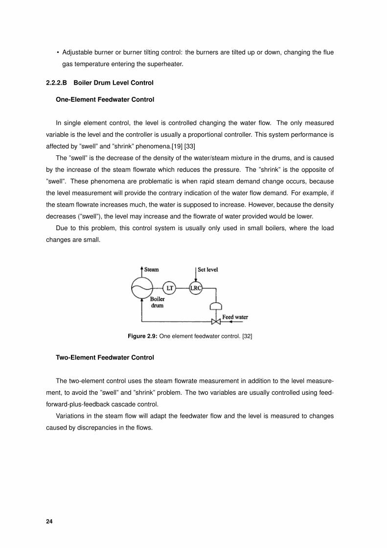
• Adjustable burner or burner tilting control: the burners are tilted up or down, changing the flue
gas temperature entering the superheater.
2.2.2.B Boiler Drum Level Control
One-Element Feedwater Control
In single element control, the level is controlled changing the water flow. The only measured
variable is the level and the controller is usually a proportional controller. This system performance is
affected by ”swell” and ”shrink” phenomena.[19] [33]
The ”swell” is the decrease of the density of the water/steam mixture in the drums, and is caused
by the increase of the steam flowrate which reduces the pressure. The ”shrink” is the opposite of
”swell”. These phenomena are problematic is when rapid steam demand change occurs, because
the level measurement will provide the contrary indication of the water flow demand. For example, if
the steam flowrate increases much, the water is supposed to increase. However, because the density
decreases (”swell”), the level may increase and the flowrate of water provided would be lower.
Due to this problem, this control system is usually only used in small boilers, where the load
changes are small.
Figure 2.9: One element feedwater control. [32]
Two-Element Feedwater Control
The two-element control uses the steam flowrate measurement in addition to the level measure-
ment, to avoid the ”swell” and ”shrink” problem. The two variables are usually controlled using feed-
forward-plus-feedback cascade control.
Variations in the steam flow will adapt the feedwater flow and the level is measured to changes
caused by discrepancies in the flows.
24
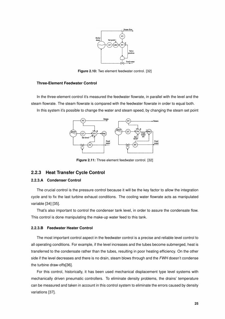
Figure 2.10: Two element feedwater control. [32]
Three-Element Feedwater Control
In the three-element control it’s measured the feedwater flowrate, in parallel with the level and the
steam flowrate. The steam flowrate is compared with the feedwater flowrate in order to equal both.
In this system it’s possible to change the water and steam speed, by changing the steam set point
Figure 2.11: Three element feedwater control. [32]
2.2.3 Heat Transfer Cycle Control
2.2.3.A Condenser Control
The crucial control is the pressure control because it will be the key factor to allow the integration
cycle and to fix the last turbine exhaust conditions. The cooling water flowrate acts as manipulated
variable [34] [35].
That’s also important to control the condenser tank level, in order to assure the condensate flow.
This control is done manipulating the make-up water feed to this tank.
2.2.3.B Feedwater Heater Control
The most important control aspect in the feedwater control is a precise and reliable level control to
all operating conditions. For example, if the level increases and the tubes become submerged, heat is
transferred to the condensate rather than the tubes, resulting in poor heating efficiency. On the other
side if the level decreases and there is no drain, steam blows through and the FWH doesn’t condense
the turbine draw-offs[36].
For this control, historically, it has been used mechanical displacement type level systems with
mechanically driven pneumatic controllers. To eliminate density problems, the drains’ temperature
can be measured and taken in account in this control system to eliminate the errors caused by density
variations [37].
25
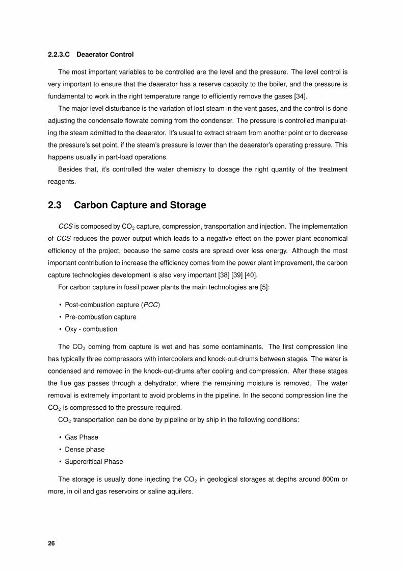
2.2.3.C Deaerator Control
The most important variables to be controlled are the level and the pressure. The level control is
very important to ensure that the deaerator has a reserve capacity to the boiler, and the pressure is
fundamental to work in the right temperature range to efficiently remove the gases [34].
The major level disturbance is the variation of lost steam in the vent gases, and the control is done
adjusting the condensate flowrate coming from the condenser. The pressure is controlled manipulat-
ing the steam admitted to the deaerator. It’s usual to extract stream from another point or to decrease
the pressure’s set point, if the steam’s pressure is lower than the deaerator’s operating pressure. This
happens usually in part-load operations.
Besides that, it’s controlled the water chemistry to dosage the right quantity of the treatment
reagents.
2.3 Carbon Capture and Storage
CCS is composed by CO2 capture, compression, transportation and injection. The implementation
of CCS reduces the power output which leads to a negative effect on the power plant economical
efficiency of the project, because the same costs are spread over less energy. Although the most
important contribution to increase the efficiency comes from the power plant improvement, the carbon
capture technologies development is also very important [38] [39] [40].
For carbon capture in fossil power plants the main technologies are [5]:
• Post-combustion capture (PCC)
• Pre-combustion capture
• Oxy - combustion
The CO2 coming from capture is wet and has some contaminants. The first compression line
has typically three compressors with intercoolers and knock-out-drums between stages. The water is
condensed and removed in the knock-out-drums after cooling and compression. After these stages
the flue gas passes through a dehydrator, where the remaining moisture is removed. The water
removal is extremely important to avoid problems in the pipeline. In the second compression line the
CO2 is compressed to the pressure required.
CO2 transportation can be done by pipeline or by ship in the following conditions:
• Gas Phase
• Dense phase
• Supercritical Phase
The storage is usually done injecting the CO2 in geological storages at depths around 800m or
more, in oil and gas reservoirs or saline aquifers.
26
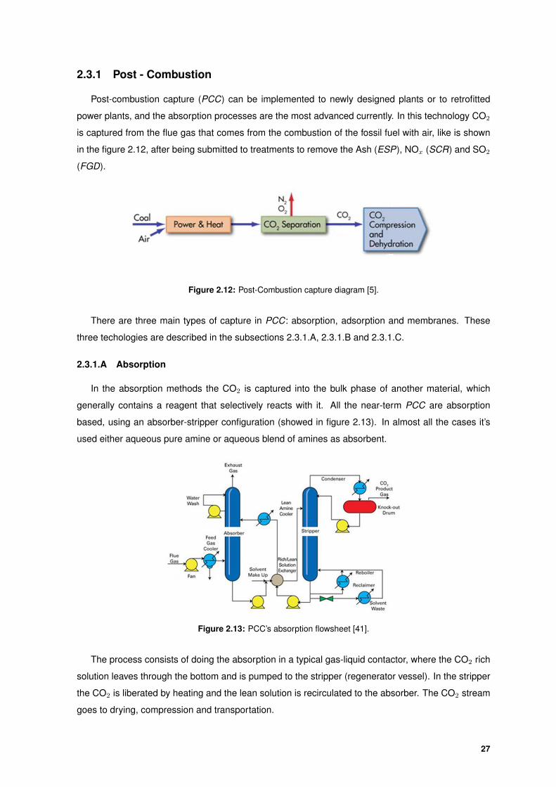
2.3.1 Post - Combustion
Post-combustion capture (PCC) can be implemented to newly designed plants or to retrofitted
power plants, and the absorption processes are the most advanced currently. In this technology CO2
is captured from the flue gas that comes from the combustion of the fossil fuel with air, like is shown
in the figure 2.12, after being submitted to treatments to remove the Ash (ESP), NOx (SCR) and SO2
(FGD).
Figure 2.12: Post-Combustion capture diagram [5].
There are three main types of capture in PCC: absorption, adsorption and membranes. These
three techologies are described in the subsections 2.3.1.A, 2.3.1.B and 2.3.1.C.
2.3.1.A Absorption
In the absorption methods the CO2 is captured into the bulk phase of another material, which
generally contains a reagent that selectively reacts with it. All the near-term PCC are absorption
based, using an absorber-stripper configuration (showed in figure 2.13). In almost all the cases it’s
used either aqueous pure amine or aqueous blend of amines as absorbent.
Figure 2.13: PCC’s absorption flowsheet [41].
The process consists of doing the absorption in a typical gas-liquid contactor, where the CO2 rich
solution leaves through the bottom and is pumped to the stripper (regenerator vessel). In the stripper
the CO2 is liberated by heating and the lean solution is recirculated to the absorber. The CO2 stream
goes to drying, compression and transportation.
27
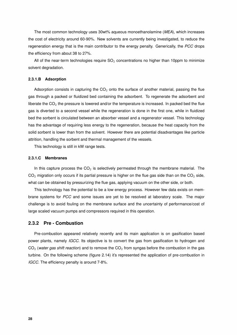
The most common technology uses 30wt% aqueous monoethanolamine (MEA), which increases
the cost of electricity around 60-90%. New solvents are currently being investigated, to reduce the
regeneration energy that is the main contributor to the energy penalty. Generically, the PCC drops
the efficiency from about 38 to 27%.
All of the near-term technologies require SO2 concentrations no higher than 10ppm to minimize
solvent degradation.
2.3.1.B Adsorption
Adsorption consists in capturing the CO2 onto the surface of another material, passing the flue
gas through a packed or fluidized bed containing the adsorbent. To regenerate the adsorbent and
liberate the CO2 the pressure is lowered and/or the temperature is increased. In packed bed the flue
gas is diverted to a second vessel while the regeneration is done in the first one, while in fluidized
bed the sorbent is circulated between an absorber vessel and a regenerator vessel. This technology
has the advantage of requiring less energy to the regeneration, because the heat capacity from the
solid sorbent is lower than from the solvent. However there are potential disadvantages like particle
attrition, handling the sorbent and thermal management of the vessels.
This technology is still in kW range tests.
2.3.1.C Membranes
In this capture process the CO2 is selectively permeated through the membrane material. The
CO2 migration only occurs if its partial pressure is higher on the flue gas side than on the CO2 side,
what can be obtained by pressurizing the flue gas, applying vacuum on the other side, or both.
This technology has the potential to be a low energy process. However few data exists on mem-
brane systems for PCC and some issues are yet to be resolved at laboratory scale. The major
challenge is to avoid fouling on the membrane surface and the uncertainty of performance/cost of
large scaled vacuum pumps and compressors required in this operation.
2.3.2 Pre - Combustion
Pre-combustion appeared relatively recently and its main application is on gasification based
power plants, namely IGCC. Its objective is to convert the gas from gasification to hydrogen and
CO2 (water gas shift reaction) and to remove the CO2 from syngas before the combustion in the gas
turbine. On the following scheme (figure 2.14) it’s represented the application of pre-combustion in
IGCC. The efficiency penalty is around 7-8%.
28
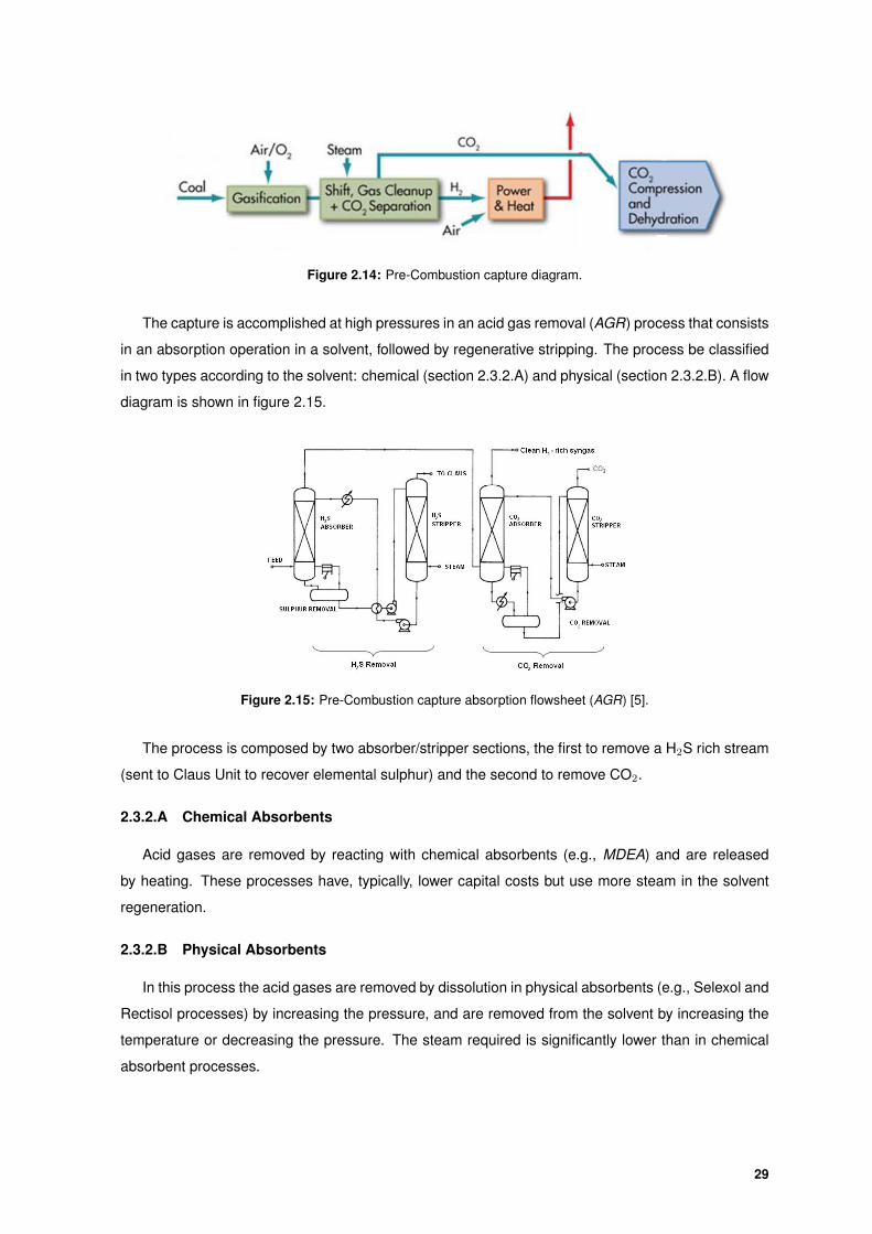
Figure 2.14: Pre-Combustion capture diagram.
The capture is accomplished at high pressures in an acid gas removal (AGR) process that consists
in an absorption operation in a solvent, followed by regenerative stripping. The process be classified
in two types according to the solvent: chemical (section 2.3.2.A) and physical (section 2.3.2.B). A flow
diagram is shown in figure 2.15.
Figure 2.15: Pre-Combustion capture absorption flowsheet (AGR) [5].
The process is composed by two absorber/stripper sections, the first to remove a H2S rich stream
(sent to Claus Unit to recover elemental sulphur) and the second to remove CO2.
2.3.2.A Chemical Absorbents
Acid gases are removed by reacting with chemical absorbents (e.g., MDEA) and are released
by heating. These processes have, typically, lower capital costs but use more steam in the solvent
regeneration.
2.3.2.B Physical Absorbents
In this process the acid gases are removed by dissolution in physical absorbents (e.g., Selexol and
Rectisol processes) by increasing the pressure, and are removed from the solvent by increasing the
temperature or decreasing the pressure. The steam required is significantly lower than in chemical
absorbent processes.
29
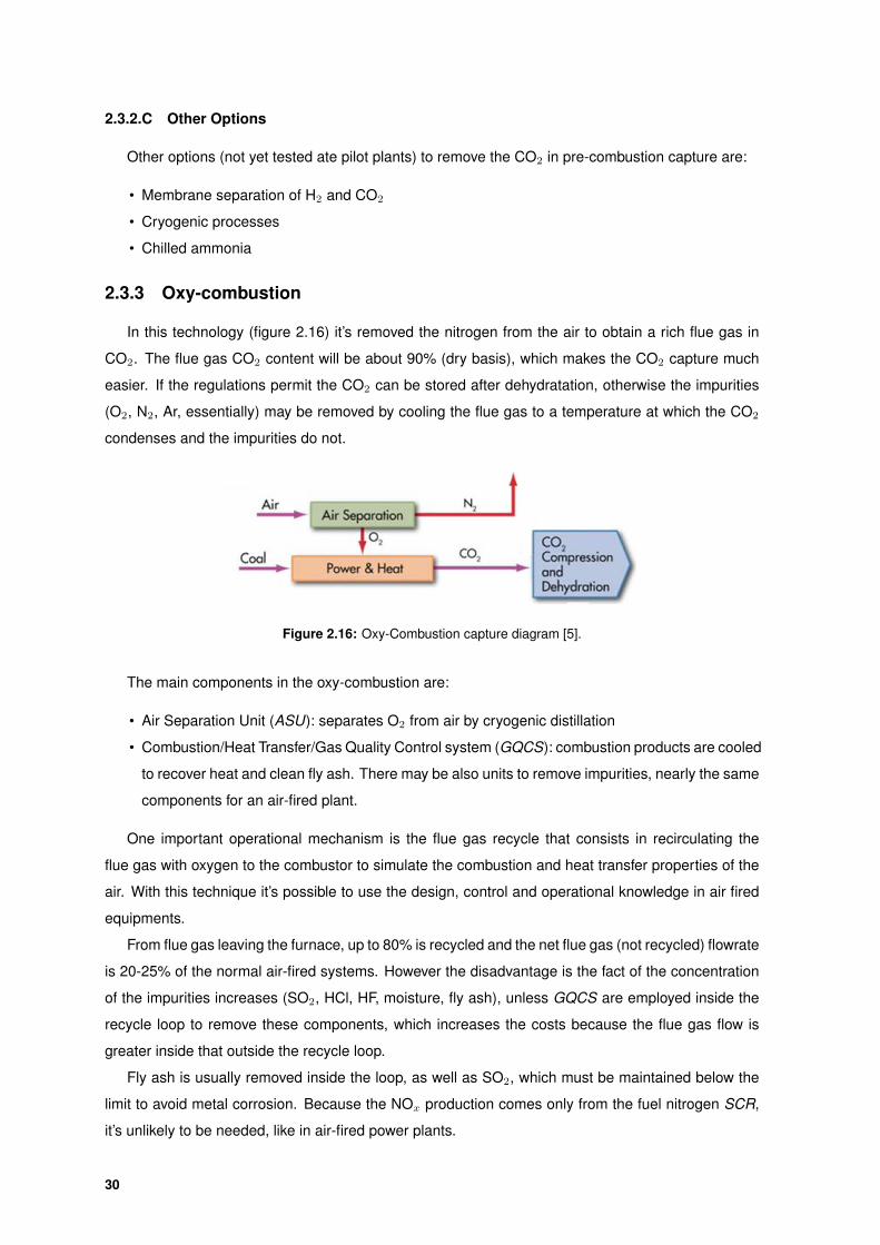
2.3.2.C Other Options
Other options (not yet tested ate pilot plants) to remove the CO2 in pre-combustion capture are:
• Membrane separation of H2 and CO2
• Cryogenic processes
• Chilled ammonia
2.3.3 Oxy-combustion
In this technology (figure 2.16) it’s removed the nitrogen from the air to obtain a rich flue gas in
CO2. The flue gas CO2 content will be about 90% (dry basis), which makes the CO2 capture much
easier. If the regulations permit the CO2 can be stored after dehydratation, otherwise the impurities
(O2, N2, Ar, essentially) may be removed by cooling the flue gas to a temperature at which the CO2
condenses and the impurities do not.
Figure 2.16: Oxy-Combustion capture diagram [5].
The main components in the oxy-combustion are:
• Air Separation Unit (ASU): separates O2 from air by cryogenic distillation
• Combustion/Heat Transfer/Gas Quality Control system (GQCS): combustion products are cooled
to recover heat and clean fly ash. There may be also units to remove impurities, nearly the same
components for an air-fired plant.
One important operational mechanism is the flue gas recycle that consists in recirculating the
flue gas with oxygen to the combustor to simulate the combustion and heat transfer properties of the
air. With this technique it’s possible to use the design, control and operational knowledge in air fired
equipments.
From flue gas leaving the furnace, up to 80% is recycled and the net flue gas (not recycled) flowrate
is 20-25% of the normal air-fired systems. However the disadvantage is the fact of the concentration
of the impurities increases (SO2, HCl, HF, moisture, fly ash), unless GQCS are employed inside the
recycle loop to remove these components, which increases the costs because the flue gas flow is
greater inside that outside the recycle loop.
Fly ash is usually removed inside the loop, as well as SO2, which must be maintained below the
limit to avoid metal corrosion. Because the NOx production comes only from the fuel nitrogen SCR,
it’s unlikely to be needed, like in air-fired power plants.
30
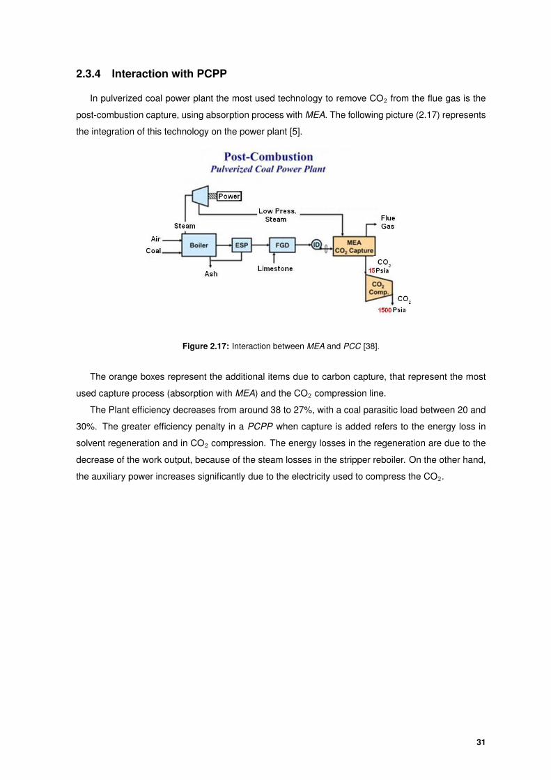
2.3.4 Interaction with PCPP
In pulverized coal power plant the most used technology to remove CO2 from the flue gas is the
post-combustion capture, using absorption process with MEA. The following picture (2.17) represents
the integration of this technology on the power plant [5].
Figure 2.17: Interaction between MEA and PCC [38].
The orange boxes represent the additional items due to carbon capture, that represent the most
used capture process (absorption with MEA) and the CO2 compression line.
The Plant efficiency decreases from around 38 to 27%, with a coal parasitic load between 20 and
30%. The greater efficiency penalty in a PCPP when capture is added refers to the energy loss in
solvent regeneration and in CO2 compression. The energy losses in the regeneration are due to the
decrease of the work output, because of the steam losses in the stripper reboiler. On the other hand,
the auxiliary power increases significantly due to the electricity used to compress the CO2.
31
3Modelling PCPP components
Contents3.1 Deaerator . . . . . . . . . . . . . . . . . . . . . . . . . . . . . . . . . . . . . . . . . . 343.2 SCR (Selective Catalytic Reduction) . . . . . . . . . . . . . . . . . . . . . . . . . . 363.3 Blower . . . . . . . . . . . . . . . . . . . . . . . . . . . . . . . . . . . . . . . . . . . . 423.4 Controller . . . . . . . . . . . . . . . . . . . . . . . . . . . . . . . . . . . . . . . . . . 453.5 Drum . . . . . . . . . . . . . . . . . . . . . . . . . . . . . . . . . . . . . . . . . . . . 48
32
In this chapter there are the models developed by the author of the thesis: Deaerator (3.1), SCR
(3.2), Blower (3.3), Controller (3.4) and Drum (3.5). All the models used to develop the final flowsheets
are summarized in the tables 4.8 and 4.2.
In the gCCS project a standard and organized methodology was followed to develop each model
the most reliably possible.
To begin, for the models where relevant information is needed, it’s done a background review
concerning the unit that the model represent, to understand the relationships that describe it and the
assumptions to make.
In the next phase it’s done a first scratch of the model, writing the equations, variables and pa-
rameters that express it. Knowing all the equations, variables and parameters it’s possible to do the
degrees of freedom, taking in account for it the model architecture, also done, to know what variables
are ”assigned” from the ports (inlet stream, e.g.).
After the DOF analysis it’s choosen the specification options, that are the variable(s) that the user
has to specify to solve the problem. For example, the specification may differ either if is being done
design or operation of the unit.
To finish the building phase it’s written the equations, variables and parameters and it’s done the
interface (ports that allow connecting the model with other ones), the specification dialog (interface
where the user does the specifications) and the report (interface where the user can see the simulation
results).
The next phase is the test and validation that is done running the models to a wide range of
conditions to debug the problems that may appear to make the model the most robust possible. It’s
also done a simulation to compare the results with real data.
In parallel with the model development, it’s created a Model Specification Document (MSD) that
describes all the model details.
An important detail on the models contruction are the variables on the connections. The material
gCCS connections ”transport” the stream’s mass flowrate, pressure, temperature, composition and
enthalpy, and these are the variables that are possible to import to the model and required to export to
the outlet connection. For example, if there is needed an inlet temperature it’s obtained directly from
the port or using a thermodynamics foreign object that relates the temperature with the pressure,
enthalpy and composition. This is why it’s equivalent to say that to solve a model is needed either the
temperature or the enthalpy, because with one of them the other is obtained.
In this chapter it’s described each model structure (inlet and outlet ports), also the degree of
freedom analysis and finally it’s shown the specification options. To do the DOF analysis there are
summarized the variables and the equations. A list of the parameters used in the equations is also
presented with their meaning.
In general all the model assumptions and special relations can be seen in the units description in
the chapter 2.1.
33
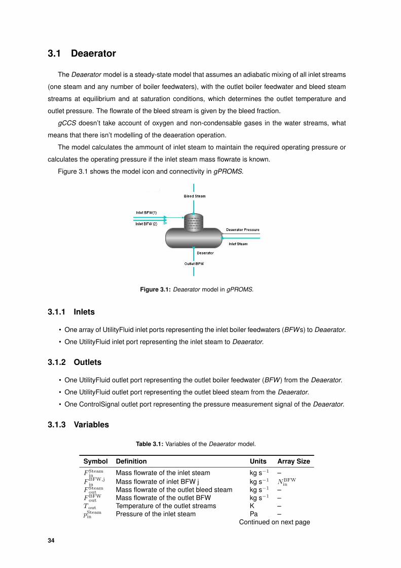
3.1 Deaerator
The Deaerator model is a steady-state model that assumes an adiabatic mixing of all inlet streams
(one steam and any number of boiler feedwaters), with the outlet boiler feedwater and bleed steam
streams at equilibrium and at saturation conditions, which determines the outlet temperature and
outlet pressure. The flowrate of the bleed stream is given by the bleed fraction.
gCCS doesn’t take account of oxygen and non-condensable gases in the water streams, what
means that there isn’t modelling of the deaeration operation.
The model calculates the ammount of inlet steam to maintain the required operating pressure or
calculates the operating pressure if the inlet steam mass flowrate is known.
Figure 3.1 shows the model icon and connectivity in gPROMS.
Figure 3.1: Deaerator model in gPROMS.
3.1.1 Inlets
• One array of UtilityFluid inlet ports representing the inlet boiler feedwaters (BFWs) to Deaerator.
• One UtilityFluid inlet port representing the inlet steam to Deaerator.
3.1.2 Outlets
• One UtilityFluid outlet port representing the outlet boiler feedwater (BFW ) from the Deaerator.
• One UtilityFluid outlet port representing the outlet bleed steam from the Deaerator.
• One ControlSignal outlet port representing the pressure measurement signal of the Deaerator.
3.1.3 Variables
Table 3.1: Variables of the Deaerator model.
Symbol Definition Units Array Size
F Steamin Mass flowrate of the inlet steam kg s−1 –
FBFW,jin Mass flowrate of inlet BFW j kg s−1 NBFW
in
F Steamout Mass flowrate of the outlet bleed steam kg s−1 –
FBFWout Mass flowrate of the outlet BFW kg s−1 –
T out Temperature of the outlet streams K –pSteam
in Pressure of the inlet steam Pa –Continued on next page
34
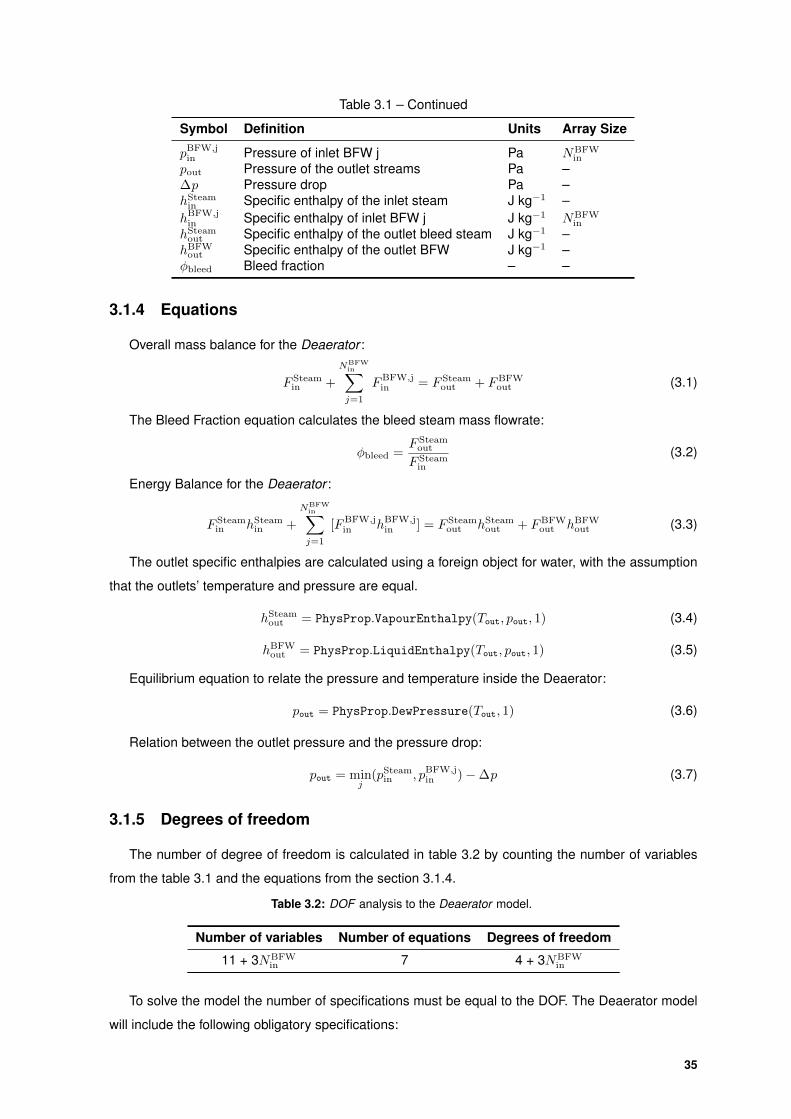
Table 3.1 – Continued
Symbol Definition Units Array Size
pBFW,jin Pressure of inlet BFW j Pa NBFW
in
pout Pressure of the outlet streams Pa –∆p Pressure drop Pa –hSteam
in Specific enthalpy of the inlet steam J kg−1 –hBFW,j
in Specific enthalpy of inlet BFW j J kg−1 NBFWin
hSteamout Specific enthalpy of the outlet bleed steam J kg−1 –hBFW
out Specific enthalpy of the outlet BFW J kg−1 –φbleed Bleed fraction – –
3.1.4 Equations
Overall mass balance for the Deaerator :
F Steamin +
NBFWin∑j=1
FBFW,jin = F Steam
out + FBFWout (3.1)
The Bleed Fraction equation calculates the bleed steam mass flowrate:
φbleed =F Steam
out
F Steamin
(3.2)
Energy Balance for the Deaerator :
F Steamin hSteam
in +
NBFWin∑j=1
[FBFW,jin hBFW,j
in ] = F Steamout hSteam
out + FBFWout hBFW
out (3.3)
The outlet specific enthalpies are calculated using a foreign object for water, with the assumption
that the outlets’ temperature and pressure are equal.
hSteamout = PhysProp.VapourEnthalpy(Tout, pout, 1) (3.4)
hBFWout = PhysProp.LiquidEnthalpy(Tout, pout, 1) (3.5)
Equilibrium equation to relate the pressure and temperature inside the Deaerator:
pout = PhysProp.DewPressure(Tout, 1) (3.6)
Relation between the outlet pressure and the pressure drop:
pout = minj
(pSteamin , pBFW,j
in )−∆p (3.7)
3.1.5 Degrees of freedom
The number of degree of freedom is calculated in table 3.2 by counting the number of variables
from the table 3.1 and the equations from the section 3.1.4.
Table 3.2: DOF analysis to the Deaerator model.
Number of variables Number of equations Degrees of freedom
11 + 3NBFWin 7 4 + 3NBFW
in
To solve the model the number of specifications must be equal to the DOF. The Deaerator model
will include the following obligatory specifications:
35
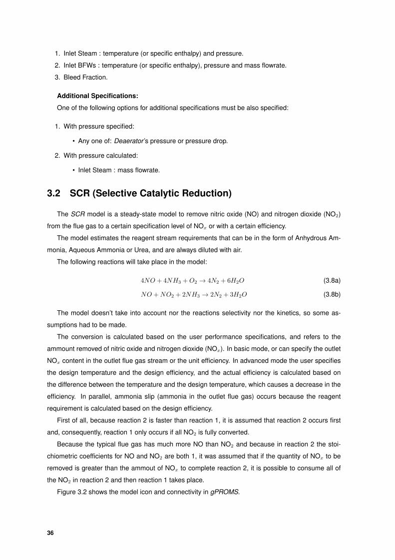
1. Inlet Steam : temperature (or specific enthalpy) and pressure.
2. Inlet BFWs : temperature (or specific enthalpy), pressure and mass flowrate.
3. Bleed Fraction.
Additional Specifications:
One of the following options for additional specifications must be also specified:
1. With pressure specified:
• Any one of: Deaerator ’s pressure or pressure drop.
2. With pressure calculated:
• Inlet Steam : mass flowrate.
3.2 SCR (Selective Catalytic Reduction)
The SCR model is a steady-state model to remove nitric oxide (NO) and nitrogen dioxide (NO2)
from the flue gas to a certain specification level of NOx or with a certain efficiency.
The model estimates the reagent stream requirements that can be in the form of Anhydrous Am-
monia, Aqueous Ammonia or Urea, and are always diluted with air.
The following reactions will take place in the model:
4NO + 4NH3 +O2 → 4N2 + 6H2O (3.8a)
NO +NO2 + 2NH3 → 2N2 + 3H2O (3.8b)
The model doesn’t take into account nor the reactions selectivity nor the kinetics, so some as-
sumptions had to be made.
The conversion is calculated based on the user performance specifications, and refers to the
ammount removed of nitric oxide and nitrogen dioxide (NOx). In basic mode, or can specify the outlet
NOx content in the outlet flue gas stream or the unit efficiency. In advanced mode the user specifies
the design temperature and the design efficiency, and the actual efficiency is calculated based on
the difference between the temperature and the design temperature, which causes a decrease in the
efficiency. In parallel, ammonia slip (ammonia in the outlet flue gas) occurs because the reagent
requirement is calculated based on the design efficiency.
First of all, because reaction 2 is faster than reaction 1, it is assumed that reaction 2 occurs first
and, consequently, reaction 1 only occurs if all NO2 is fully converted.
Because the typical flue gas has much more NO than NO2 and because in reaction 2 the stoi-
chiometric coefficients for NO and NO2 are both 1, it was assumed that if the quantity of NOx to be
removed is greater than the ammout of NOx to complete reaction 2, it is possible to consume all of
the NO2 in reaction 2 and then reaction 1 takes place.
Figure 3.2 shows the model icon and connectivity in gPROMS.
36
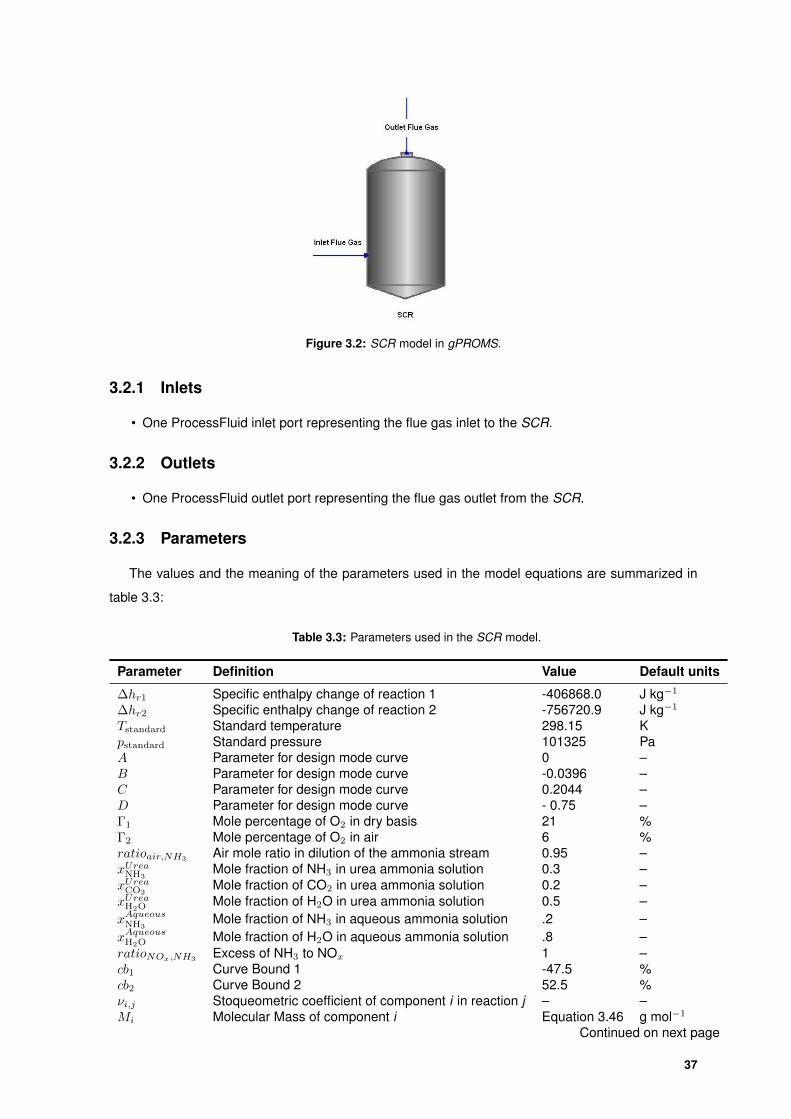
Figure 3.2: SCR model in gPROMS.
3.2.1 Inlets
• One ProcessFluid inlet port representing the flue gas inlet to the SCR.
3.2.2 Outlets
• One ProcessFluid outlet port representing the flue gas outlet from the SCR.
3.2.3 Parameters
The values and the meaning of the parameters used in the model equations are summarized in
table 3.3:
Table 3.3: Parameters used in the SCR model.
Parameter Definition Value Default units
∆hr1 Specific enthalpy change of reaction 1 -406868.0 J kg−1
∆hr2 Specific enthalpy change of reaction 2 -756720.9 J kg−1
Tstandard Standard temperature 298.15 Kpstandard Standard pressure 101325 PaA Parameter for design mode curve 0 –B Parameter for design mode curve -0.0396 –C Parameter for design mode curve 0.2044 –D Parameter for design mode curve - 0.75 –Γ1 Mole percentage of O2 in dry basis 21 %Γ2 Mole percentage of O2 in air 6 %ratioair,NH3 Air mole ratio in dilution of the ammonia stream 0.95 –xUreaNH3
Mole fraction of NH3 in urea ammonia solution 0.3 –xUreaCO2
Mole fraction of CO2 in urea ammonia solution 0.2 –xUreaH2O Mole fraction of H2O in urea ammonia solution 0.5 –xAqueousNH3
Mole fraction of NH3 in aqueous ammonia solution .2 –xAqueousH2O Mole fraction of H2O in aqueous ammonia solution .8 –ratioNOx,NH3
Excess of NH3 to NOx 1 –cb1 Curve Bound 1 -47.5 %cb2 Curve Bound 2 52.5 %νi,j Stoqueometric coefficient of component i in reaction j – –Mi Molecular Mass of component i Equation 3.46 g mol−1
Continued on next page
37
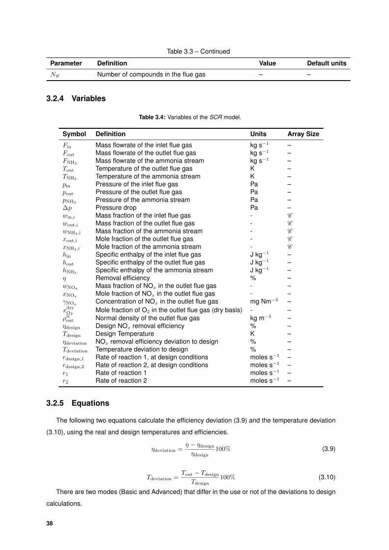
Table 3.3 – Continued
Parameter Definition Value Default units
NC Number of compounds in the flue gas – –
3.2.4 Variables
Table 3.4: Variables of the SCR model.
Symbol Definition Units Array Size
Fin Mass flowrate of the inlet flue gas kg s−1 –Fout Mass flowrate of the outlet flue gas kg s−1 –FNH3 Mass flowrate of the ammonia stream kg s−1 –Tout Temperature of the outlet flue gas K –TNH3
Temperature of the ammonia stream K –pin Pressure of the inlet flue gas Pa –pout Pressure of the outlet flue gas Pa –pNH3
Pressure of the ammonia stream Pa –∆p Pressure drop Pa –win,i Mass fraction of the inlet flue gas - Cwout,i Mass fraction of the outlet flue gas - CwNH3,i Mass fraction of the ammonia stream - Cxout,i Mole fraction of the outlet flue gas - CxNH3,i Mole fraction of the ammonia stream - Chin Specific enthalpy of the inlet flue gas J kg−1 –hout Specific enthalpy of the outlet flue gas J kg−1 –hNH3
Specific enthalpy of the ammonia stream J kg−1 –η Removal efficiency % –wNOx
Mass fraction of NOx in the outlet flue gas - –xNOx Mole fraction of NOx in the outlet flue gas - –γNOx Concentration of NOx in the outlet flue gas mg Nm−3 –xdry
O2Mole fraction of O2 in the outlet flue gas (dry basis) - –
ρNout Normal density of the outlet flue gas kg m−3 –ηdesign Design NOx removal efficiency % –Tdesign Design Temperature K –ηdeviation NOx removal efficiency deviation to design % –Tdeviation Temperature deviation to design % –rdesign,1 Rate of reaction 1, at design conditions moles s−1 –rdesign,2 Rate of reaction 2, at design conditions moles s−1 –r1 Rate of reaction 1 moles s−1 –r2 Rate of reaction 2 moles s−1 –
3.2.5 Equations
The following two equations calculate the efficiency deviation (3.9) and the temperature deviation
(3.10), using the real and design temperatures and efficiencies.
ηdeviation =η − ηdesign
ηdesign100% (3.9)
Tdeviation =Tout − Tdesign
Tdesign100% (3.10)
There are two modes (Basic and Advanced) that differ in the use or not of the deviations to design
calculations.
38
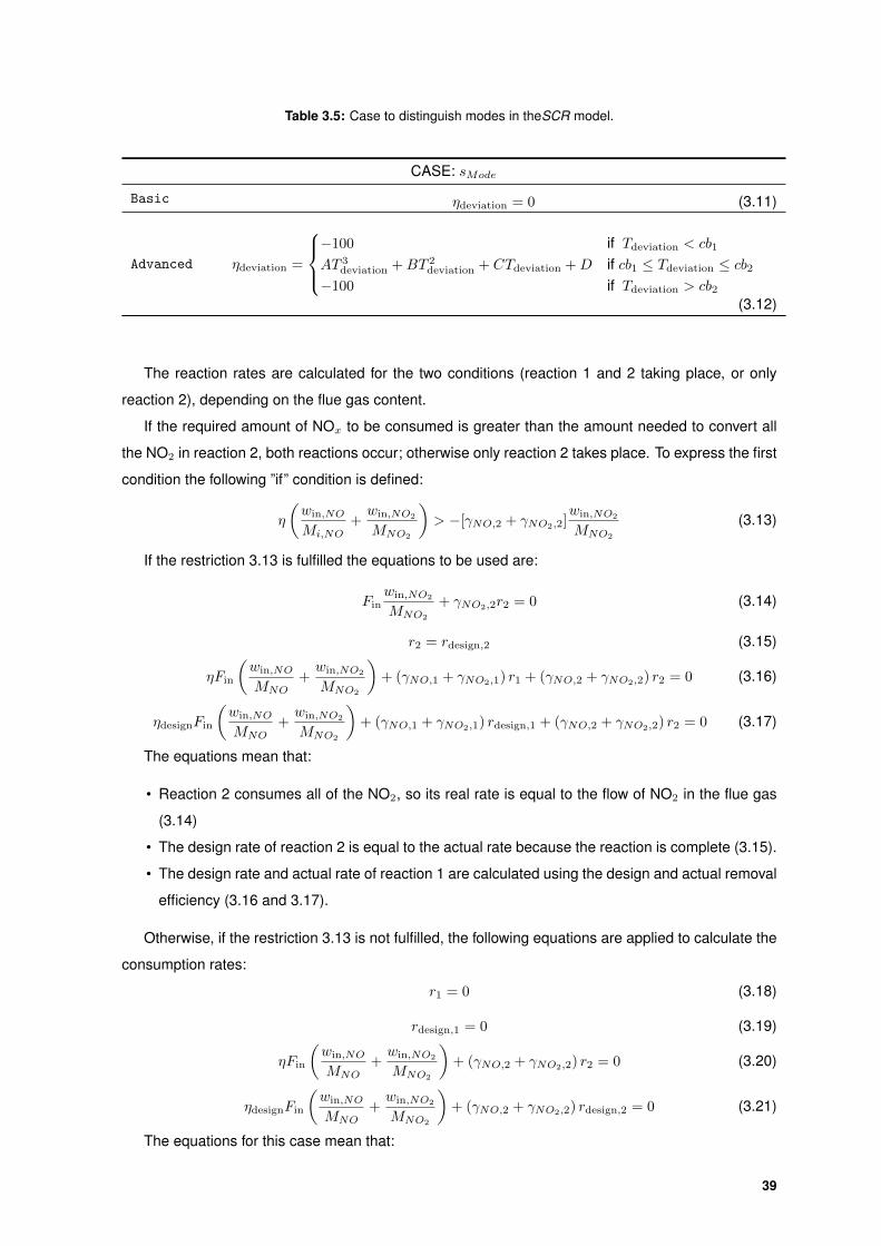
Table 3.5: Case to distinguish modes in theSCR model.
CASE: sMode
Basic ηdeviation = 0 (3.11)
Advanced ηdeviation =
−100 if Tdeviation < cb1
AT 3deviation +BT 2
deviation + CTdeviation +D if cb1 ≤ Tdeviation ≤ cb2−100 if Tdeviation > cb2
(3.12)
The reaction rates are calculated for the two conditions (reaction 1 and 2 taking place, or only
reaction 2), depending on the flue gas content.
If the required amount of NOx to be consumed is greater than the amount needed to convert all
the NO2 in reaction 2, both reactions occur; otherwise only reaction 2 takes place. To express the first
condition the following ”if” condition is defined:
η
(win,NO
Mi,NO+win,NO2
MNO2
)> −[γNO,2 + γNO2,2]
win,NO2
MNO2
(3.13)
If the restriction 3.13 is fulfilled the equations to be used are:
Finwin,NO2
MNO2
+ γNO2,2r2 = 0 (3.14)
r2 = rdesign,2 (3.15)
ηFin
(win,NO
MNO+win,NO2
MNO2
)+ (γNO,1 + γNO2,1) r1 + (γNO,2 + γNO2,2) r2 = 0 (3.16)
ηdesignFin
(win,NO
MNO+win,NO2
MNO2
)+ (γNO,1 + γNO2,1) rdesign,1 + (γNO,2 + γNO2,2) r2 = 0 (3.17)
The equations mean that:
• Reaction 2 consumes all of the NO2, so its real rate is equal to the flow of NO2 in the flue gas
(3.14)
• The design rate of reaction 2 is equal to the actual rate because the reaction is complete (3.15).
• The design rate and actual rate of reaction 1 are calculated using the design and actual removal
efficiency (3.16 and 3.17).
Otherwise, if the restriction 3.13 is not fulfilled, the following equations are applied to calculate the
consumption rates:
r1 = 0 (3.18)
rdesign,1 = 0 (3.19)
ηFin
(win,NO
MNO+win,NO2
MNO2
)+ (γNO,2 + γNO2,2) r2 = 0 (3.20)
ηdesignFin
(win,NO
MNO+win,NO2
MNO2
)+ (γNO,2 + γNO2,2) rdesign,2 = 0 (3.21)
The equations for this case mean that:
39
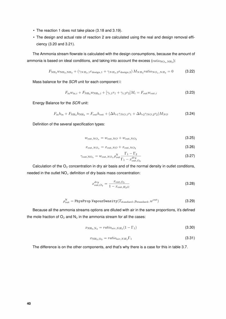
• The reaction 1 does not take place (3.18 and 3.19).
• The design and actual rate of reaction 2 are calculated using the real and design removal effi-
ciency (3.20 and 3.21).
The Ammonia stream flowrate is calculated with the design consumptions, because the amount of
ammonia is based on ideal conditions, and taking into account the excess (ratioNOx,NH3):
FNH3wNH3,NH3 + (γNH3,1rdesign,1 + γNH3,2rdesign,2)MNH3ratioNOx,NH3 = 0 (3.22)
Mass balance for the SCR unit for each component i:
Finwin,i + FNH3wNH3,i + [γi,1r1 + γi,2r2]Mi = Foutwout,i (3.23)
Energy Balance for the SCR unit:
Finhin + FNH3hNH3
= Fouthout + (∆hr1γNO,1r1 + ∆hr2γNO,2r2)MNO (3.24)
Definition of the several specification types:
wout,NOx= wout,NO + wout,NO2
(3.25)
xout,NOx= xout,NO + xout,NO2
(3.26)
γout,NOx = wout,NOxρNout
Γ1 − Γ2
Γ1 − xdryout,O2
(3.27)
Calculation of the O2 concentration in dry air basis and of the normal density in outlet conditions,
needed in the outlet NOx definition of dry basis mass concentration:
xdryout,O2=
xout,O2
1− xout,H2O(3.28)
ρNout = PhysProp.VapourDensity(Tstandard, pstandard, w
out) (3.29)
Because all the ammonia streams options are diluted with air in the same proportions, it’s defined
the mole fraction of O2 and N2 in the ammonia stream for all the cases:
xNH3,N2= ratioair,NH3
(1− Γ1) (3.30)
xNH3,O2 = ratioair,NH3Γ1 (3.31)
The difference is on the other components, and that’s why there is a case for this in table 3.7.
40
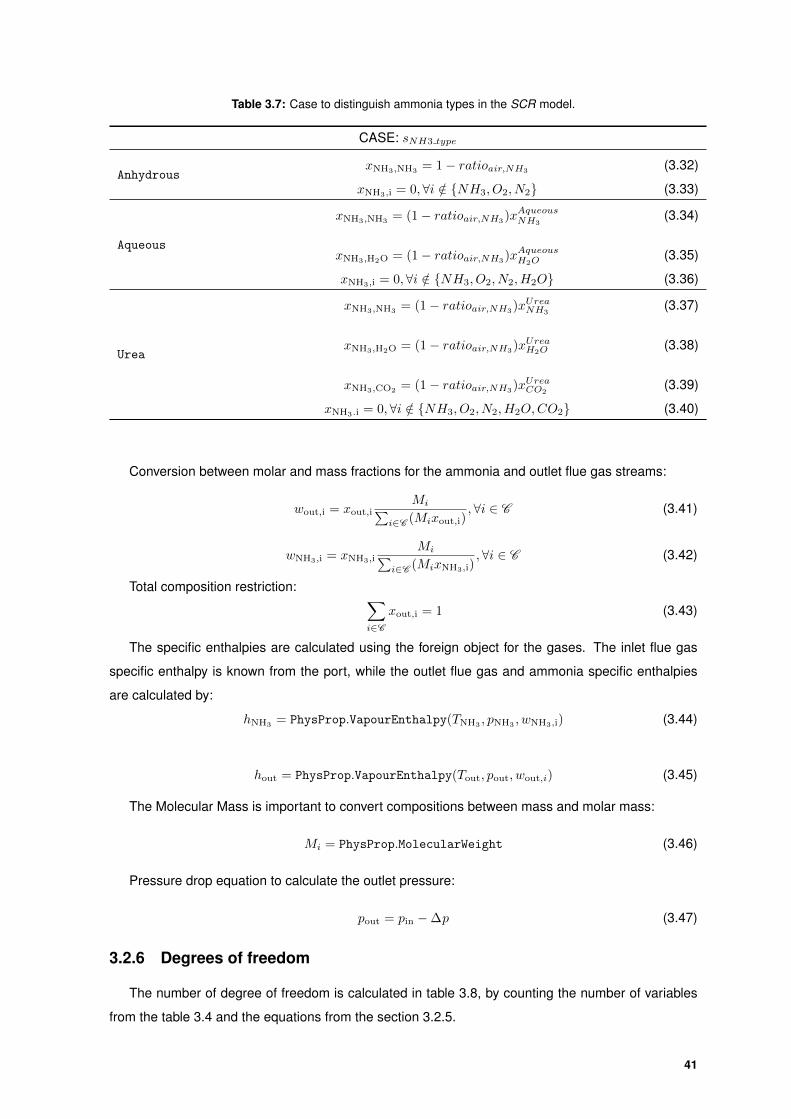
Table 3.7: Case to distinguish ammonia types in the SCR model.
CASE: sNH3 type
AnhydrousxNH3,NH3
= 1− ratioair,NH3(3.32)
xNH3,i = 0,∀i /∈ {NH3, O2, N2} (3.33)
Aqueous
xNH3,NH3= (1− ratioair,NH3
)xAqueousNH3(3.34)
xNH3,H2O = (1− ratioair,NH3)xAqueousH2O
(3.35)
xNH3,i = 0,∀i /∈ {NH3, O2, N2, H2O} (3.36)
Urea
xNH3,NH3 = (1− ratioair,NH3)xUreaNH3(3.37)
xNH3,H2O = (1− ratioair,NH3)xUreaH2O (3.38)
xNH3,CO2 = (1− ratioair,NH3)xUreaCO2(3.39)
xNH3.i = 0,∀i /∈ {NH3, O2, N2, H2O,CO2} (3.40)
Conversion between molar and mass fractions for the ammonia and outlet flue gas streams:
wout,i = xout,iMi∑
i∈C (Mixout,i),∀i ∈ C (3.41)
wNH3,i = xNH3,iMi∑
i∈C (MixNH3,i),∀i ∈ C (3.42)
Total composition restriction: ∑i∈C
xout,i = 1 (3.43)
The specific enthalpies are calculated using the foreign object for the gases. The inlet flue gas
specific enthalpy is known from the port, while the outlet flue gas and ammonia specific enthalpies
are calculated by:
hNH3= PhysProp.VapourEnthalpy(TNH3
, pNH3, wNH3,i) (3.44)
hout = PhysProp.VapourEnthalpy(Tout, pout, wout,i) (3.45)
The Molecular Mass is important to convert compositions between mass and molar mass:
Mi = PhysProp.MolecularWeight (3.46)
Pressure drop equation to calculate the outlet pressure:
pout = pin −∆p (3.47)
3.2.6 Degrees of freedom
The number of degree of freedom is calculated in table 3.8, by counting the number of variables
from the table 3.4 and the equations from the section 3.2.5.
41
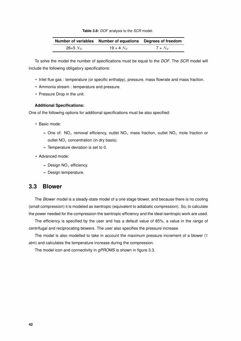
Table 3.8: DOF analysis to the SCR model.
Number of variables Number of equations Degrees of freedom
26+5 NC 19 + 4 NC 7 + NC
To solve the model the number of specifications must be equal to the DOF. The SCR model will
include the following obligatory specifications:
• Inlet flue gas : temperature (or specific enthalpy), pressure, mass flowrate and mass fraction.
• Ammonia stream : temperature and pressure.
• Pressure Drop in the unit.
Additional Specifications:
One of the following options for additional specifications must be also specified:
• Basic mode:
– One of: NOx removal efficiency, outlet NOx mass fraction, outlet NOx mole fraction or
outlet NOx concentration (in dry basis).
– Temperature deviation is set to 0.
• Advanced mode:
– Design NOx efficiency.
– Design temperature.
3.3 Blower
The Blower model is a steady-state model of a one stage blower, and because there is no cooling
(small compression) it is modeled as isentropic (equivalent to adiabatic compression). So, to calculate
the power needed for the compression the isentropic efficiency and the ideal isentropic work are used.
The efficiency is specified by the user and has a default value of 85%, a value in the range of
centrifugal and reciprocating blowers. The user also specifies the pressure increase.
The model is also modelled to take in account the maximum pressure increment of a blower (1
atm) and calculates the temperature increase during the compression.
The model icon and connectivity in gPROMS is shown in figure 3.3.
42
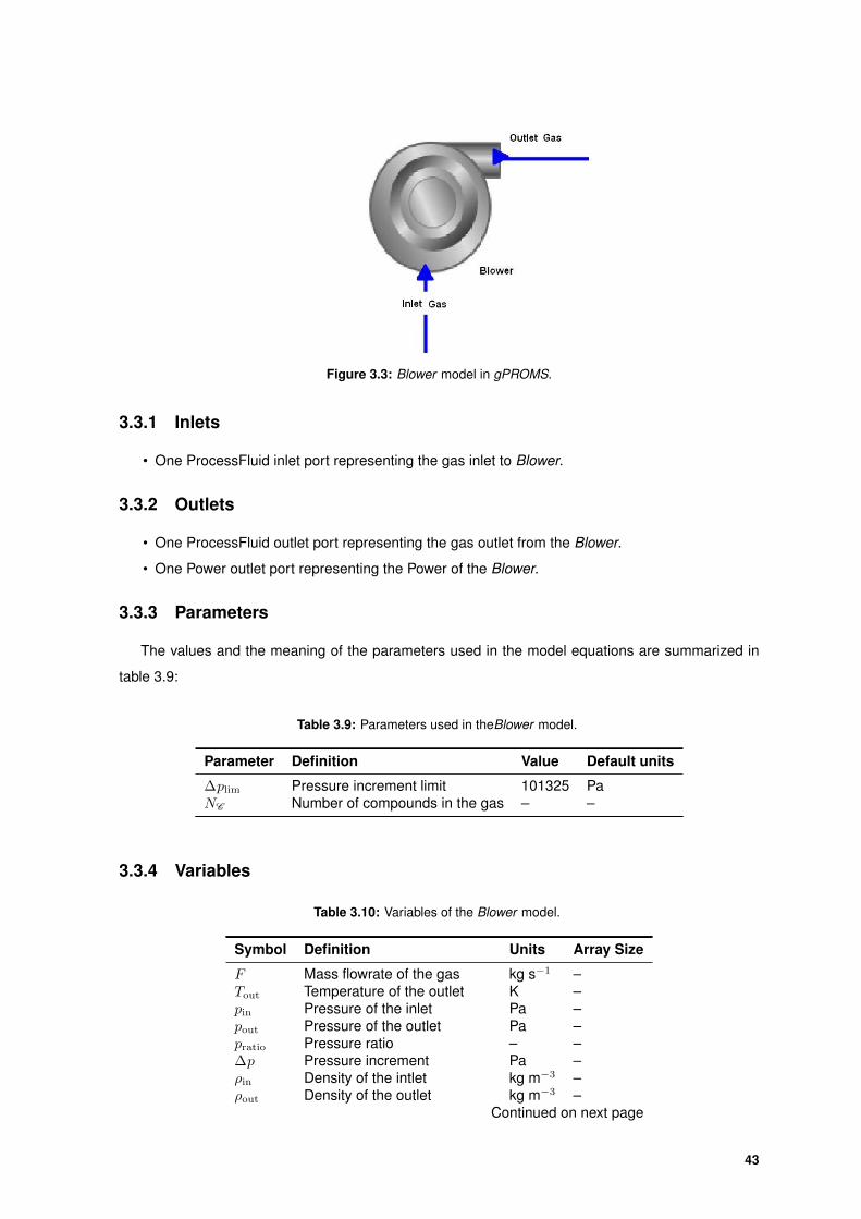
Figure 3.3: Blower model in gPROMS.
3.3.1 Inlets
• One ProcessFluid inlet port representing the gas inlet to Blower.
3.3.2 Outlets
• One ProcessFluid outlet port representing the gas outlet from the Blower.
• One Power outlet port representing the Power of the Blower.
3.3.3 Parameters
The values and the meaning of the parameters used in the model equations are summarized in
table 3.9:
Table 3.9: Parameters used in theBlower model.
Parameter Definition Value Default units
∆plim Pressure increment limit 101325 PaNC Number of compounds in the gas – –
3.3.4 Variables
Table 3.10: Variables of the Blower model.
Symbol Definition Units Array Size
F Mass flowrate of the gas kg s−1 –Tout Temperature of the outlet K –pin Pressure of the inlet Pa –pout Pressure of the outlet Pa –pratio Pressure ratio – –∆p Pressure increment Pa –ρin Density of the intlet kg m−3 –ρout Density of the outlet kg m−3 –
Continued on next page
43
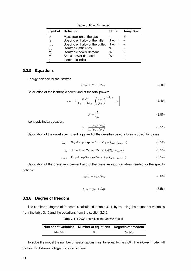
Table 3.10 – Continued
Symbol Definition Units Array Size
wi Mass fraction of the gas – Chin Specific enthalpy of the intlet J kg−1 –hout Specific enthalpy of the outlet J kg−1 –ηis Isentropic efficiency % –Pis Isentropic power demand W –P Actual power demand W –γ Isentropic index – –
3.3.5 Equations
Energy balance for the Blower :
Fhin + P = Fhout (3.48)
Calculation of the isentropic power and of the total power:
Pis = Fpinγ
(γ − 1)ρin
[(pout
pin
)1−1/γ
− 1
](3.49)
P =Pis
ηis(3.50)
Isentropic index equation:
γ =ln (pout/pin)
ln (ρout/ρin)(3.51)
Calculation of the outlet specific enthalpy and of the densities using a foreign object for gases:
hout = PhysProp.VapourEnthalpy(Tout, pout, w) (3.52)
ρin = PhysProp.VapourDensity(Tin, pin, w) (3.53)
ρout = PhysProp.VapourDensity(Tout, pout, w) (3.54)
Calculation of the pressure increment and of the pressure ratio, variables needed for the specifi-
cations:
pratio = pout/pin (3.55)
pout = pin + ∆p (3.56)
3.3.6 Degree of freedom
The number of degree of freedom is calculated in table 3.11, by counting the number of variables
from the table 3.10 and the equations from the section 3.3.5.
Table 3.11: DOF analysis to the Blower model.
Number of variables Number of equations Degrees of freedom
14+ NC 9 5+ NC
To solve the model the number of specifications must be equal to the DOF. The Blower model will
include the following obligatory specifications:
44
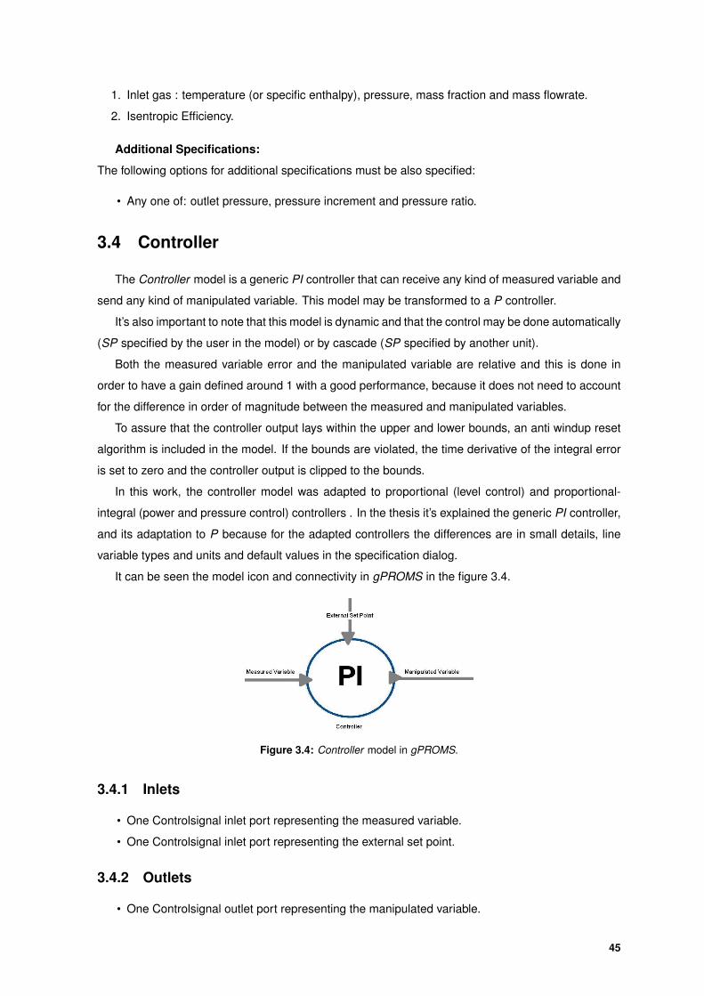
1. Inlet gas : temperature (or specific enthalpy), pressure, mass fraction and mass flowrate.
2. Isentropic Efficiency.
Additional Specifications:
The following options for additional specifications must be also specified:
• Any one of: outlet pressure, pressure increment and pressure ratio.
3.4 Controller
The Controller model is a generic PI controller that can receive any kind of measured variable and
send any kind of manipulated variable. This model may be transformed to a P controller.
It’s also important to note that this model is dynamic and that the control may be done automatically
(SP specified by the user in the model) or by cascade (SP specified by another unit).
Both the measured variable error and the manipulated variable are relative and this is done in
order to have a gain defined around 1 with a good performance, because it does not need to account
for the difference in order of magnitude between the measured and manipulated variables.
To assure that the controller output lays within the upper and lower bounds, an anti windup reset
algorithm is included in the model. If the bounds are violated, the time derivative of the integral error
is set to zero and the controller output is clipped to the bounds.
In this work, the controller model was adapted to proportional (level control) and proportional-
integral (power and pressure control) controllers . In the thesis it’s explained the generic PI controller,
and its adaptation to P because for the adapted controllers the differences are in small details, line
variable types and units and default values in the specification dialog.
It can be seen the model icon and connectivity in gPROMS in the figure 3.4.
Figure 3.4: Controller model in gPROMS.
3.4.1 Inlets
• One Controlsignal inlet port representing the measured variable.
• One Controlsignal inlet port representing the external set point.
3.4.2 Outlets
• One Controlsignal outlet port representing the manipulated variable.
45
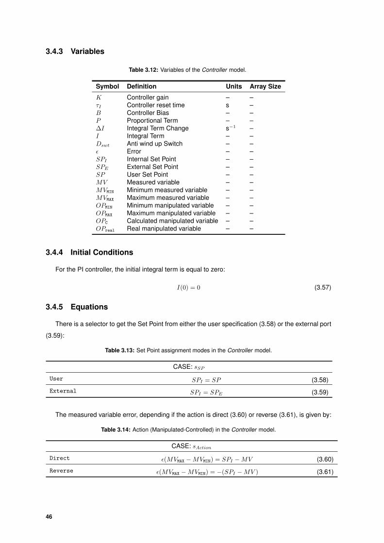
3.4.3 Variables
Table 3.12: Variables of the Controller model.
Symbol Definition Units Array Size
K Controller gain – –τI Controller reset time s –B Controller Bias – –P Proportional Term – –∆I Integral Term Change s−1 –I Integral Term – –Dswt Anti wind up Switch – –ε Error – –SPI Internal Set Point – –SPE External Set Point – –SP User Set Point – –MV Measured variable – –MVMIN Minimum measured variable – –MVMAX Maximum measured variable – –OPMIN Minimum manipulated variable – –OPMAX Maximum manipulated variable – –OPC Calculated manipulated variable – –OPreal Real manipulated variable – –
3.4.4 Initial Conditions
For the PI controller, the initial integral term is equal to zero:
I(0) = 0 (3.57)
3.4.5 Equations
There is a selector to get the Set Point from either the user specification (3.58) or the external port
(3.59):
Table 3.13: Set Point assignment modes in the Controller model.
CASE: sSP
User SPI = SP (3.58)
External SPI = SPE (3.59)
The measured variable error, depending if the action is direct (3.60) or reverse (3.61), is given by:
Table 3.14: Action (Manipulated-Controlled) in the Controller model.
CASE: sAction
Direct ε(MVMAX −MVMIN) = SPI −MV (3.60)
Reverse ε(MVMAX −MVMIN) = −(SPI −MV ) (3.61)
46
For a proportional-integral Controller the control equation becomes:
OPC = K(P + I)(OPMAX −OPMIN) +B (3.62)
With the proportional term:
P = ε (3.63)
In order to integrate the error in the PI controlller it’s used the equation:
dI
dt=
ε
τI(3.64)
To a P Controller the integral term is set to zero:
I = 0 (3.65)
The real manipulated value is constrained by its maximum and minimum values:
OPreal = max[OPMIN,min(OPMAX, OPC)] (3.66)
The anti windup reset algorithm consits in a selector that turns off and on the integral action:
∆I =
{EτI
if OPMIN −Dsw > OP > OPMAX +Dsw
0 otherwise(3.67)
3.4.6 Degree of freedom
The number of degree of freedom is calculated in table 3.15, by counting the number of variables
from the table 3.12 and the equations from the section 3.4.5.
Table 3.15: DOF analysis to the Controller model.
Number of variables Number of equations Degrees of freedom
18 9 9
To solve the model the number of specifications must be equal to the DOF. The Controller will
include the following obligatory specifications:
1. Measured variable : signal.
2. Controller:
• Action : direct or reverse.
• Controller parameters : gain, bias, maximum and minimum input and maximum and mini-
mum output.
Additional Specifications:
The following options for additional specifications must be also specified:
1. Proportional Controller:
• External Set-Point mode:
47
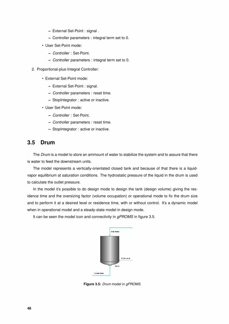
– External Set-Point : signal .
– Controller parameters : integral term set to 0.
• User Set-Point mode:
– Controller : Set-Point.
– Controller parameters : integral term set to 0.
2. Proportional-plus-Integral Controller:
• External Set-Point mode:
– External Set-Point : signal.
– Controller parameters : reset time.
– StopIntegrator : active or inactive.
• User Set-Point mode:
– Controller : Set-Point.
– Controller parameters : reset time.
– StopIntegrator : active or inactive.
3.5 Drum
The Drum is a model to store an ammount of water to stabilize the system and to assure that there
is water to feed the downstream units.
The model represents a vertically-orientated closed tank and because of that there is a liquid-
vapor equilibrium at saturation conditions. The hydrostatic pressure of the liquid in the drum is used
to calculate the outlet pressure.
In the model it’s possible to do design mode to design the tank (design volume) giving the res-
idence time and the oversizing factor (volume occupation) or operational mode to fix the drum size
and to perform it at a desired level or residence time, with or without control. It’s a dynamic model
when in operational model and a steady-state model in design mode.
It can be seen the model icon and connectivity in gPROMS in figure 3.5.
Figure 3.5: Drum model in gPROMS.
48
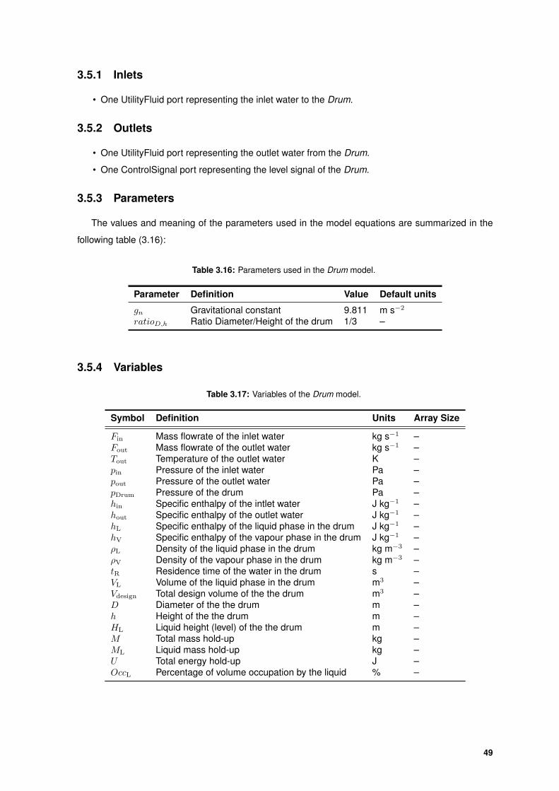
3.5.1 Inlets
• One UtilityFluid port representing the inlet water to the Drum.
3.5.2 Outlets
• One UtilityFluid port representing the outlet water from the Drum.
• One ControlSignal port representing the level signal of the Drum.
3.5.3 Parameters
The values and meaning of the parameters used in the model equations are summarized in the
following table (3.16):
Table 3.16: Parameters used in the Drum model.
Parameter Definition Value Default units
gn Gravitational constant 9.811 m s−2
ratioD,h Ratio Diameter/Height of the drum 1/3 –
3.5.4 Variables
Table 3.17: Variables of the Drum model.
Symbol Definition Units Array Size
Fin Mass flowrate of the inlet water kg s−1 –Fout Mass flowrate of the outlet water kg s−1 –Tout Temperature of the outlet water K –pin Pressure of the inlet water Pa –pout Pressure of the outlet water Pa –pDrum Pressure of the drum Pa –hin Specific enthalpy of the intlet water J kg−1 –hout Specific enthalpy of the outlet water J kg−1 –hL Specific enthalpy of the liquid phase in the drum J kg−1 –hV Specific enthalpy of the vapour phase in the drum J kg−1 –ρL Density of the liquid phase in the drum kg m−3 –ρV Density of the vapour phase in the drum kg m−3 –tR Residence time of the water in the drum s –VL Volume of the liquid phase in the drum m3 –Vdesign Total design volume of the the drum m3 –D Diameter of the the drum m –h Height of the the drum m –HL Liquid height (level) of the the drum m –M Total mass hold-up kg –ML Liquid mass hold-up kg –U Total energy hold-up J –OccL Percentage of volume occupation by the liquid % –
49
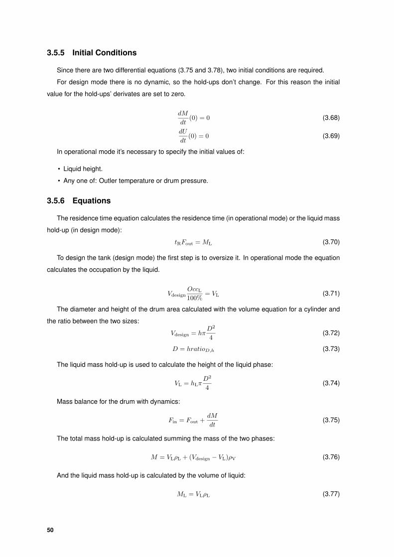
3.5.5 Initial Conditions
Since there are two differential equations (3.75 and 3.78), two initial conditions are required.
For design mode there is no dynamic, so the hold-ups don’t change. For this reason the initial
value for the hold-ups’ derivates are set to zero.
dM
dt(0) = 0 (3.68)
dU
dt(0) = 0 (3.69)
In operational mode it’s necessary to specify the initial values of:
• Liquid height.
• Any one of: Outler temperature or drum pressure.
3.5.6 Equations
The residence time equation calculates the residence time (in operational mode) or the liquid mass
hold-up (in design mode):
tRFout = ML (3.70)
To design the tank (design mode) the first step is to oversize it. In operational mode the equation
calculates the occupation by the liquid.
VdesignOccL100%
= VL (3.71)
The diameter and height of the drum area calculated with the volume equation for a cylinder and
the ratio between the two sizes:
Vdesign = hπD2
4(3.72)
D = hratioD,h (3.73)
The liquid mass hold-up is used to calculate the height of the liquid phase:
VL = hLπD2
4(3.74)
Mass balance for the drum with dynamics:
Fin = Fout +dM
dt(3.75)
The total mass hold-up is calculated summing the mass of the two phases:
M = VLρL + (Vdesign − VL)ρV (3.76)
And the liquid mass hold-up is calculated by the volume of liquid:
ML = VLρL (3.77)
50
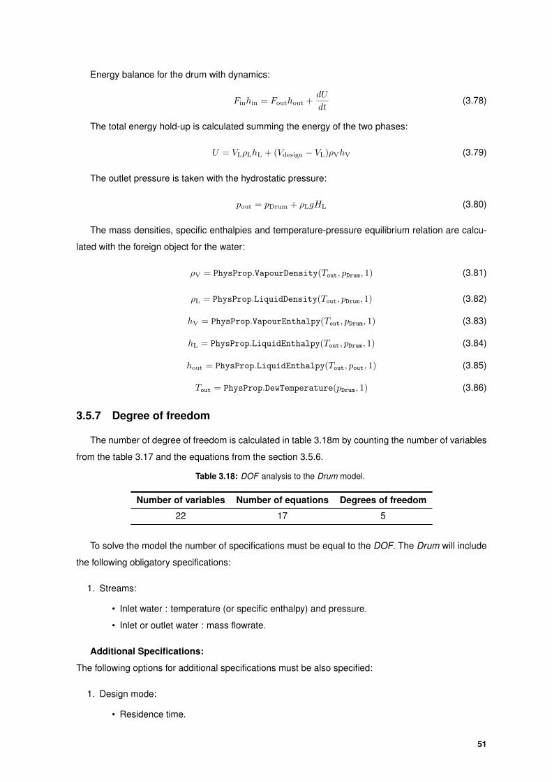
Energy balance for the drum with dynamics:
Finhin = Fouthout +dU
dt(3.78)
The total energy hold-up is calculated summing the energy of the two phases:
U = VLρLhL + (Vdesign − VL)ρVhV (3.79)
The outlet pressure is taken with the hydrostatic pressure:
pout = pDrum + ρLgHL (3.80)
The mass densities, specific enthalpies and temperature-pressure equilibrium relation are calcu-
lated with the foreign object for the water:
ρV = PhysProp.VapourDensity(Tout, pDrum, 1) (3.81)
ρL = PhysProp.LiquidDensity(Tout, pDrum, 1) (3.82)
hV = PhysProp.VapourEnthalpy(Tout, pDrum, 1) (3.83)
hL = PhysProp.LiquidEnthalpy(Tout, pDrum, 1) (3.84)
hout = PhysProp.LiquidEnthalpy(Tout, pout, 1) (3.85)
Tout = PhysProp.DewTemperature(pDrum, 1) (3.86)
3.5.7 Degree of freedom
The number of degree of freedom is calculated in table 3.18m by counting the number of variables
from the table 3.17 and the equations from the section 3.5.6.
Table 3.18: DOF analysis to the Drum model.
Number of variables Number of equations Degrees of freedom
22 17 5
To solve the model the number of specifications must be equal to the DOF. The Drum will include
the following obligatory specifications:
1. Streams:
• Inlet water : temperature (or specific enthalpy) and pressure.
• Inlet or outlet water : mass flowrate.
Additional Specifications:
The following options for additional specifications must be also specified:
1. Design mode:
• Residence time.
51

• Volume occupation.
2. Operational mode:
• Without level Control:
– Total volume.
– Residence time.
• With level Control:
– Total volume.
– Inlet or outlet water : mass flowrate (from control valve).
52

4Modelling a PCPP
Contents4.1 Design Mode . . . . . . . . . . . . . . . . . . . . . . . . . . . . . . . . . . . . . . . . 554.2 Operational Mode . . . . . . . . . . . . . . . . . . . . . . . . . . . . . . . . . . . . . 604.3 Control Mode . . . . . . . . . . . . . . . . . . . . . . . . . . . . . . . . . . . . . . . . 614.4 Sensitivity Analyses . . . . . . . . . . . . . . . . . . . . . . . . . . . . . . . . . . . . 70
53
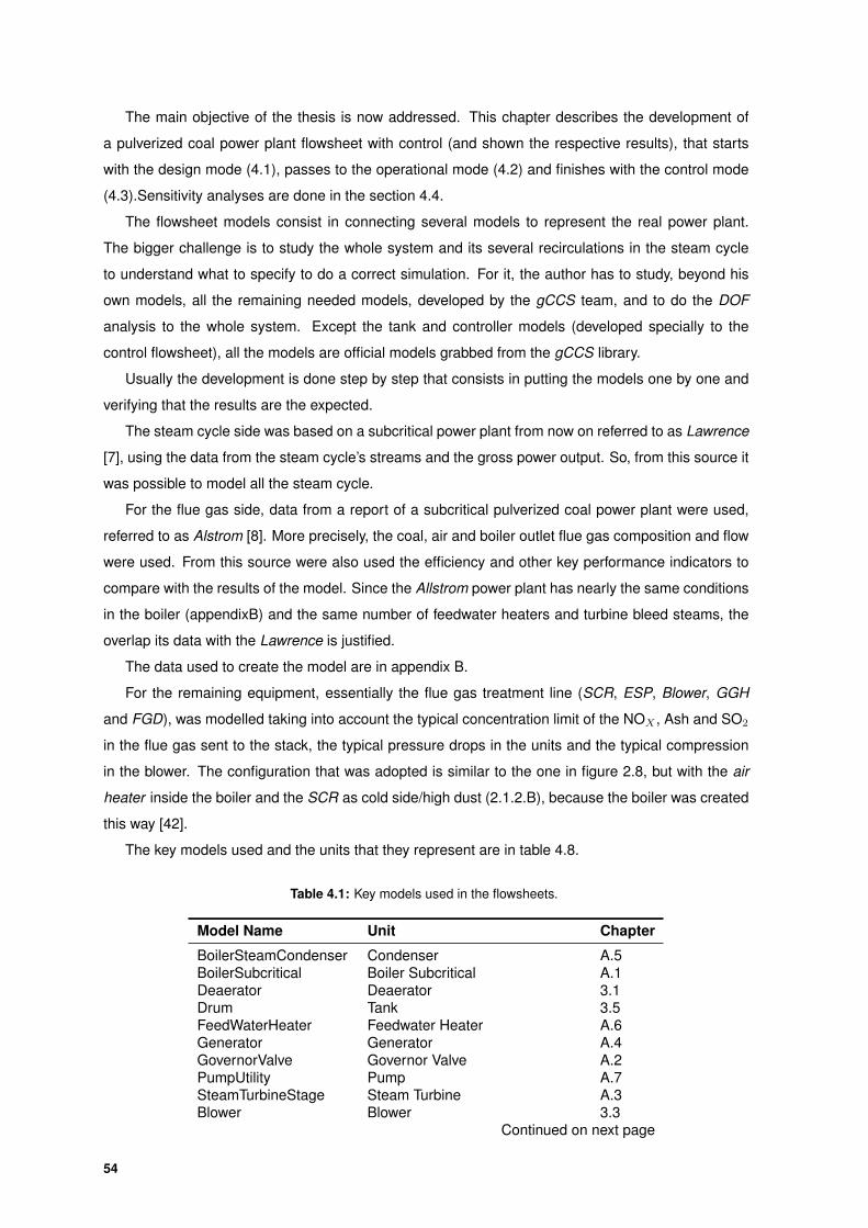
The main objective of the thesis is now addressed. This chapter describes the development of
a pulverized coal power plant flowsheet with control (and shown the respective results), that starts
with the design mode (4.1), passes to the operational mode (4.2) and finishes with the control mode
(4.3).Sensitivity analyses are done in the section 4.4.
The flowsheet models consist in connecting several models to represent the real power plant.
The bigger challenge is to study the whole system and its several recirculations in the steam cycle
to understand what to specify to do a correct simulation. For it, the author has to study, beyond his
own models, all the remaining needed models, developed by the gCCS team, and to do the DOF
analysis to the whole system. Except the tank and controller models (developed specially to the
control flowsheet), all the models are official models grabbed from the gCCS library.
Usually the development is done step by step that consists in putting the models one by one and
verifying that the results are the expected.
The steam cycle side was based on a subcritical power plant from now on referred to as Lawrence
[7], using the data from the steam cycle’s streams and the gross power output. So, from this source it
was possible to model all the steam cycle.
For the flue gas side, data from a report of a subcritical pulverized coal power plant were used,
referred to as Alstrom [8]. More precisely, the coal, air and boiler outlet flue gas composition and flow
were used. From this source were also used the efficiency and other key performance indicators to
compare with the results of the model. Since the Allstrom power plant has nearly the same conditions
in the boiler (appendixB) and the same number of feedwater heaters and turbine bleed steams, the
overlap its data with the Lawrence is justified.
The data used to create the model are in appendix B.
For the remaining equipment, essentially the flue gas treatment line (SCR, ESP, Blower, GGH
and FGD), was modelled taking into account the typical concentration limit of the NOX , Ash and SO2
in the flue gas sent to the stack, the typical pressure drops in the units and the typical compression
in the blower. The configuration that was adopted is similar to the one in figure 2.8, but with the air
heater inside the boiler and the SCR as cold side/high dust (2.1.2.B), because the boiler was created
this way [42].
The key models used and the units that they represent are in table 4.8.
Table 4.1: Key models used in the flowsheets.
Model Name Unit Chapter
BoilerSteamCondenser Condenser A.5BoilerSubcritical Boiler Subcritical A.1Deaerator Deaerator 3.1Drum Tank 3.5FeedWaterHeater Feedwater Heater A.6Generator Generator A.4GovernorValve Governor Valve A.2PumpUtility Pump A.7SteamTurbineStage Steam Turbine A.3Blower Blower 3.3
Continued on next page
54
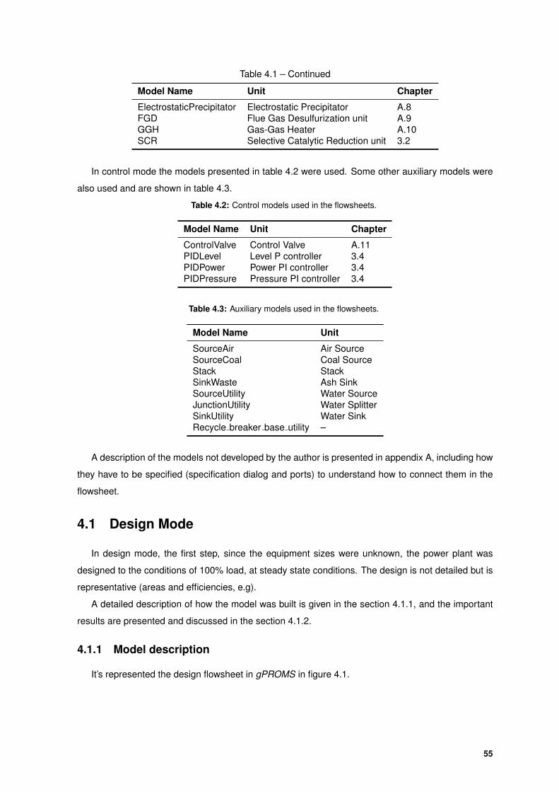
Table 4.1 – Continued
Model Name Unit Chapter
ElectrostaticPrecipitator Electrostatic Precipitator A.8FGD Flue Gas Desulfurization unit A.9GGH Gas-Gas Heater A.10SCR Selective Catalytic Reduction unit 3.2
In control mode the models presented in table 4.2 were used. Some other auxiliary models were
also used and are shown in table 4.3.
Table 4.2: Control models used in the flowsheets.
Model Name Unit Chapter
ControlValve Control Valve A.11PIDLevel Level P controller 3.4PIDPower Power PI controller 3.4PIDPressure Pressure PI controller 3.4
Table 4.3: Auxiliary models used in the flowsheets.
Model Name Unit
SourceAir Air SourceSourceCoal Coal SourceStack StackSinkWaste Ash SinkSourceUtility Water SourceJunctionUtility Water SplitterSinkUtility Water SinkRecycle breaker base utility –
A description of the models not developed by the author is presented in appendix A, including how
they have to be specified (specification dialog and ports) to understand how to connect them in the
flowsheet.
4.1 Design Mode
In design mode, the first step, since the equipment sizes were unknown, the power plant was
designed to the conditions of 100% load, at steady state conditions. The design is not detailed but is
representative (areas and efficiencies, e.g).
A detailed description of how the model was built is given in the section 4.1.1, and the important
results are presented and discussed in the section 4.1.2.
4.1.1 Model description
It’s represented the design flowsheet in gPROMS in figure 4.1.
55
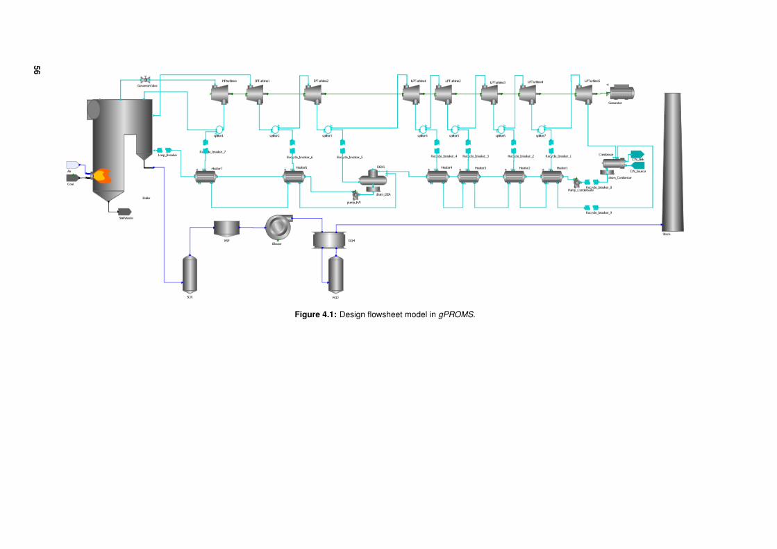
Figure 4.1: Design flowsheet model in gPROMS.
56
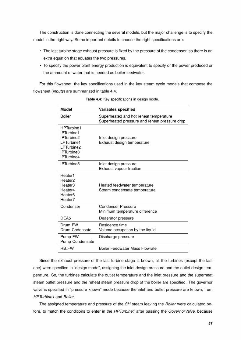
The construction is done connecting the several models, but the major challenge is to specify the
model in the right way. Some important details to choose the right specifications are:
• The last turbine stage exhaust pressure is fixed by the pressure of the condenser, so there is an
extra equation that equates the two pressures.
• To specify the power plant energy production is equivalent to specify or the power produced or
the ammount of water that is needed as boiler feedwater.
For this flowsheet, the key specifications used in the key steam cycle models that compose the
flowsheet (inputs) are summarized in table 4.4.
Table 4.4: Key specifications in design mode.
Model Variables specified
Boiler Superheated and hot reheat temperatureSuperheated pressure and reheat pressure drop
HPTurbine1IPTurbine1IPTurbine2 Inlet design pressureLPTurbine1 Exhaust design temperatureLPTurbine2IPTurbine3IPTurbine4
IPTurbine5 Inlet design pressureExhaust vapour fraction
Heater1Heater2Heater3 Heated feedwater temperatureHeater4 Steam condensate temperatureHeater6Heater7
Condenser Condenser PressureMinimum temperature difference
DEA5 Deaerator pressure
Drum FW Residence timeDrum Codensate Volume occupation by the liquid
Pump FW Discharge pressurePump Condensate
RB FW Boiler Feedwater Mass Flowrate
Since the exhaust pressure of the last turbine stage is known, all the turbines (except the last
one) were specified in “design mode”, assigning the inlet design pressure and the outlet design tem-
perature. So, the turbines calculate the outlet temperature and the inlet pressure and the superheat
steam outlet pressure and the reheat steam pressure drop of the boiler are specified. The governor
valve is specified in “pressure known” mode because the inlet and outlet pressure are known, from
HPTurbine1 and Boiler.
The assigned temperature and pressure of the SH steam leaving the Boiler were calculated be-
fore, to match the conditions to enter in the HPTurbine1 after passing the GovernorValve, because
57
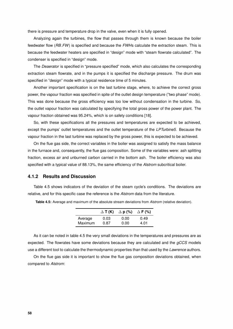
there is pressure and temperature drop in the valve, even when it is fully opened.
Analyzing again the turbines, the flow that passes through them is known because the boiler
feedwater flow (RB FW ) is specified and because the FWHs calculate the extraction steam. This is
because the feedwater heaters are specified in “design” mode with “steam flowrate calculated”. The
condenser is specified in “design” mode.
The Deaerator is specified in “pressure specified” mode, which also calculates the corresponding
extraction steam flowrate, and in the pumps it is specified the discharge pressure. The drum was
specified in ”design” mode with a typical residence time of 5 minutes.
Another important specification is on the last turbine stage, where, to achieve the correct gross
power, the vapour fraction was specified in spite of the outlet design temperature (”two phase” mode).
This was done because the gross efficiency was too low without condensation in the turbine. So,
the outlet vapour fraction was calculated by specifying the total gross power of the power plant. The
vapour fraction obtained was 95.24%, which is on safety conditions [18].
So, with these specifications all the pressures and temperatures are expected to be achieved,
except the pumps’ outlet temperatures and the outlet temperature of the LPTurbine5. Because the
vapour fraction in the last turbine was replaced by the gross power, this is expected to be achieved.
On the flue gas side, the correct variables in the boiler was assigned to satisfy the mass balance
in the furnace and, consequently, the flue gas composition. Some of the variables were: ash splitting
fraction, excess air and unburned carbon carried in the bottom ash. The boiler efficiency was also
specified with a typical value of 88.13%, the same efficiency of the Alstrom subcritical boiler.
4.1.2 Results and Discussion
Table 4.5 shows indicators of the deviation of the steam cycle’s conditions. The deviations are
relative, and for this specific case the reference is the Alstrom data from the literature.
Table 4.5: Average and maximum of the absolute stream deviations from Alstrom (relative deviation).
∆ T (K) ∆ p (%) ∆ F (%)
Average 0.03 0.00 0.49Maximum 0.87 0.00 4.01
As it can be noted in table 4.5 the very small deviations in the temperatures and pressures are as
expected. The flowrates have some deviations because they are calculated and the gCCS models
use a different tool to calculate the thermodynamic properties than that used by the Lawrence authors.
On the flue gas side it is important to show the flue gas composition deviations obtained, when
compared to Alstrom:
58
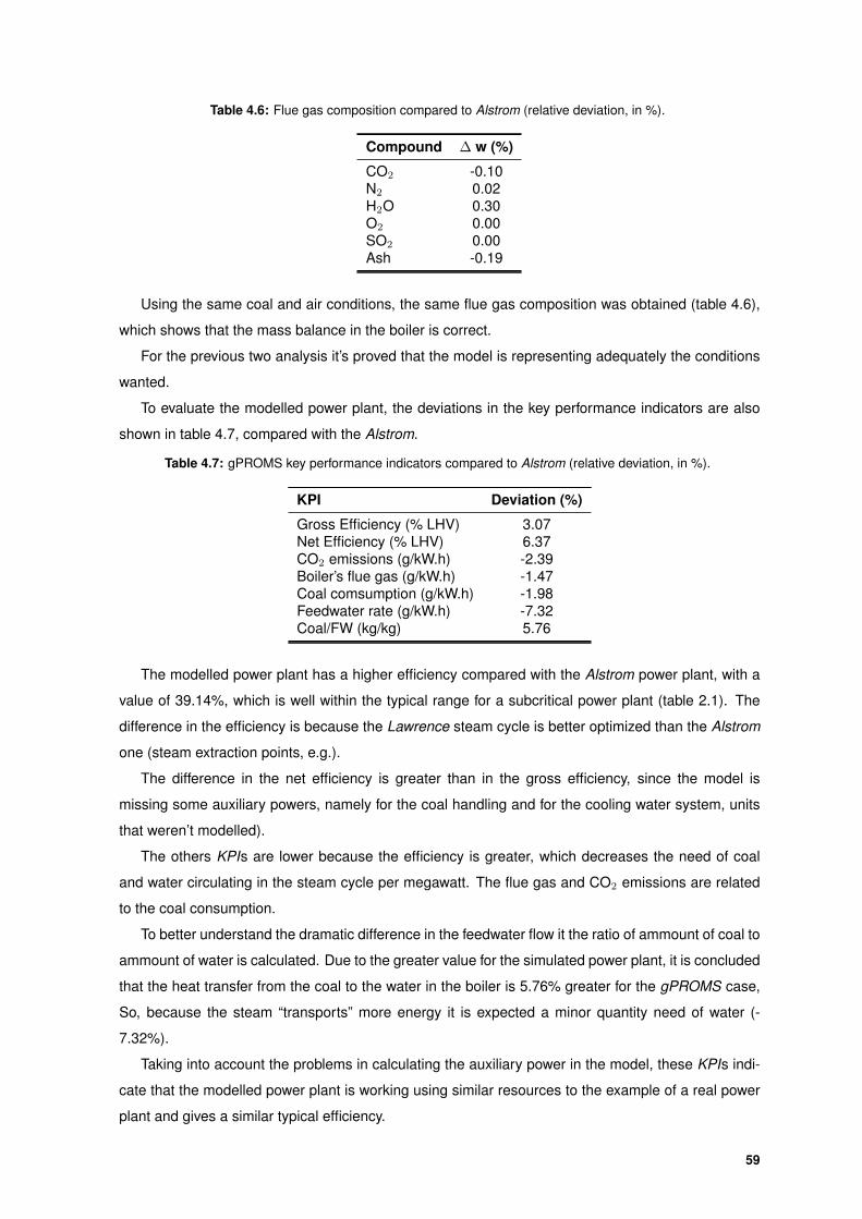
Table 4.6: Flue gas composition compared to Alstrom (relative deviation, in %).
Compound ∆ w (%)
CO2 -0.10N2 0.02H2O 0.30O2 0.00SO2 0.00Ash -0.19
Using the same coal and air conditions, the same flue gas composition was obtained (table 4.6),
which shows that the mass balance in the boiler is correct.
For the previous two analysis it’s proved that the model is representing adequately the conditions
wanted.
To evaluate the modelled power plant, the deviations in the key performance indicators are also
shown in table 4.7, compared with the Alstrom.
Table 4.7: gPROMS key performance indicators compared to Alstrom (relative deviation, in %).
KPI Deviation (%)
Gross Efficiency (% LHV) 3.07Net Efficiency (% LHV) 6.37CO2 emissions (g/kW.h) -2.39Boiler’s flue gas (g/kW.h) -1.47Coal comsumption (g/kW.h) -1.98Feedwater rate (g/kW.h) -7.32Coal/FW (kg/kg) 5.76
The modelled power plant has a higher efficiency compared with the Alstrom power plant, with a
value of 39.14%, which is well within the typical range for a subcritical power plant (table 2.1). The
difference in the efficiency is because the Lawrence steam cycle is better optimized than the Alstrom
one (steam extraction points, e.g.).
The difference in the net efficiency is greater than in the gross efficiency, since the model is
missing some auxiliary powers, namely for the coal handling and for the cooling water system, units
that weren’t modelled).
The others KPIs are lower because the efficiency is greater, which decreases the need of coal
and water circulating in the steam cycle per megawatt. The flue gas and CO2 emissions are related
to the coal consumption.
To better understand the dramatic difference in the feedwater flow it the ratio of ammount of coal to
ammount of water is calculated. Due to the greater value for the simulated power plant, it is concluded
that the heat transfer from the coal to the water in the boiler is 5.76% greater for the gPROMS case,
So, because the steam “transports” more energy it is expected a minor quantity need of water (-
7.32%).
Taking into account the problems in calculating the auxiliary power in the model, these KPIs indi-
cate that the modelled power plant is working using similar resources to the example of a real power
plant and gives a similar typical efficiency.
59
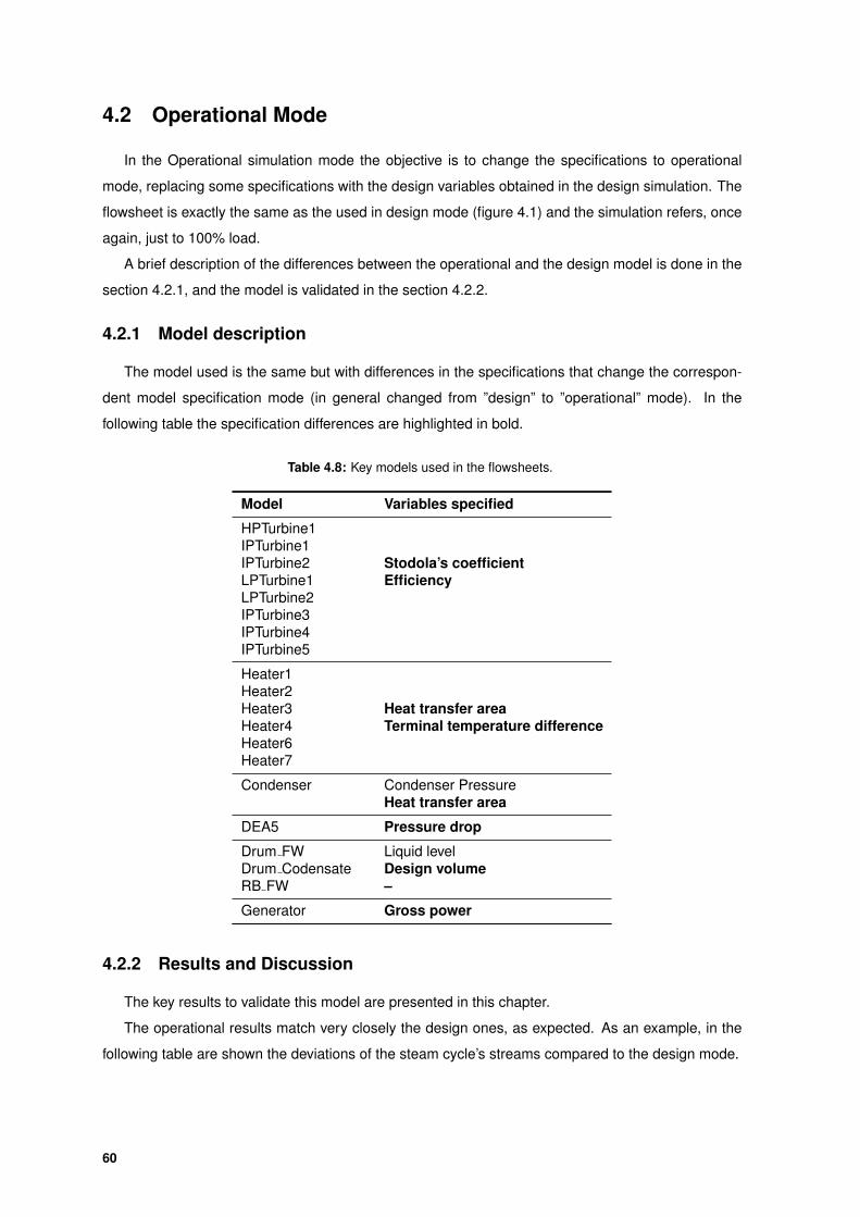
4.2 Operational Mode
In the Operational simulation mode the objective is to change the specifications to operational
mode, replacing some specifications with the design variables obtained in the design simulation. The
flowsheet is exactly the same as the used in design mode (figure 4.1) and the simulation refers, once
again, just to 100% load.
A brief description of the differences between the operational and the design model is done in the
section 4.2.1, and the model is validated in the section 4.2.2.
4.2.1 Model description
The model used is the same but with differences in the specifications that change the correspon-
dent model specification mode (in general changed from ”design” to ”operational” mode). In the
following table the specification differences are highlighted in bold.
Table 4.8: Key models used in the flowsheets.
Model Variables specified
HPTurbine1IPTurbine1IPTurbine2 Stodola’s coefficientLPTurbine1 EfficiencyLPTurbine2IPTurbine3IPTurbine4IPTurbine5
Heater1Heater2Heater3 Heat transfer areaHeater4 Terminal temperature differenceHeater6Heater7
Condenser Condenser PressureHeat transfer area
DEA5 Pressure drop
Drum FW Liquid levelDrum Codensate Design volumeRB FW –
Generator Gross power
4.2.2 Results and Discussion
The key results to validate this model are presented in this chapter.
The operational results match very closely the design ones, as expected. As an example, in the
following table are shown the deviations of the steam cycle’s streams compared to the design mode.
60
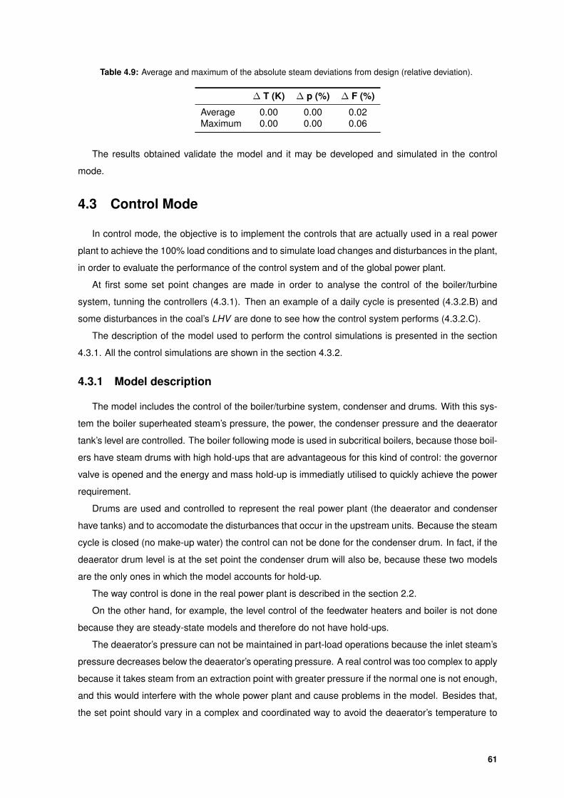
Table 4.9: Average and maximum of the absolute steam deviations from design (relative deviation).
∆ T (K) ∆ p (%) ∆ F (%)
Average 0.00 0.00 0.02Maximum 0.00 0.00 0.06
The results obtained validate the model and it may be developed and simulated in the control
mode.
4.3 Control Mode
In control mode, the objective is to implement the controls that are actually used in a real power
plant to achieve the 100% load conditions and to simulate load changes and disturbances in the plant,
in order to evaluate the performance of the control system and of the global power plant.
At first some set point changes are made in order to analyse the control of the boiler/turbine
system, tunning the controllers (4.3.1). Then an example of a daily cycle is presented (4.3.2.B) and
some disturbances in the coal’s LHV are done to see how the control system performs (4.3.2.C).
The description of the model used to perform the control simulations is presented in the section
4.3.1. All the control simulations are shown in the section 4.3.2.
4.3.1 Model description
The model includes the control of the boiler/turbine system, condenser and drums. With this sys-
tem the boiler superheated steam’s pressure, the power, the condenser pressure and the deaerator
tank’s level are controlled. The boiler following mode is used in subcritical boilers, because those boil-
ers have steam drums with high hold-ups that are advantageous for this kind of control: the governor
valve is opened and the energy and mass hold-up is immediatly utilised to quickly achieve the power
requirement.
Drums are used and controlled to represent the real power plant (the deaerator and condenser
have tanks) and to accomodate the disturbances that occur in the upstream units. Because the steam
cycle is closed (no make-up water) the control can not be done for the condenser drum. In fact, if the
deaerator drum level is at the set point the condenser drum will also be, because these two models
are the only ones in which the model accounts for hold-up.
The way control is done in the real power plant is described in the section 2.2.
On the other hand, for example, the level control of the feedwater heaters and boiler is not done
because they are steady-state models and therefore do not have hold-ups.
The deaerator’s pressure can not be maintained in part-load operations because the inlet steam’s
pressure decreases below the deaerator’s operating pressure. A real control was too complex to apply
because it takes steam from an extraction point with greater pressure if the normal one is not enough,
and this would interfere with the whole power plant and cause problems in the model. Besides that,
the set point should vary in a complex and coordinated way to avoid the deaerator’s temperature to
61
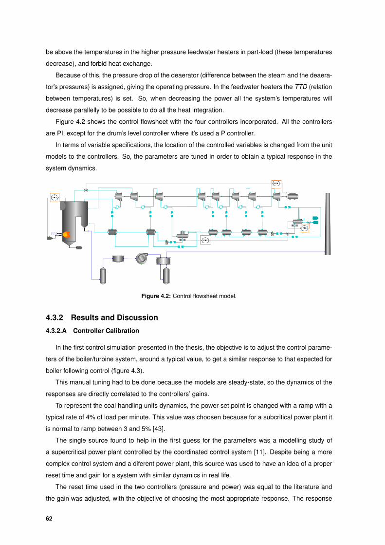
be above the temperatures in the higher pressure feedwater heaters in part-load (these temperatures
decrease), and forbid heat exchange.
Because of this, the pressure drop of the deaerator (difference between the steam and the deaera-
tor’s pressures) is assigned, giving the operating pressure. In the feedwater heaters the TTD (relation
between temperatures) is set. So, when decreasing the power all the system’s temperatures will
decrease parallelly to be possible to do all the heat integration.
Figure 4.2 shows the control flowsheet with the four controllers incorporated. All the controllers
are PI, except for the drum’s level controller where it’s used a P controller.
In terms of variable specifications, the location of the controlled variables is changed from the unit
models to the controllers. So, the parameters are tuned in order to obtain a typical response in the
system dynamics.
Figure 4.2: Control flowsheet model.
4.3.2 Results and Discussion
4.3.2.A Controller Calibration
In the first control simulation presented in the thesis, the objective is to adjust the control parame-
ters of the boiler/turbine system, around a typical value, to get a similar response to that expected for
boiler following control (figure 4.3).
This manual tuning had to be done because the models are steady-state, so the dynamics of the
responses are directly correlated to the controllers’ gains.
To represent the coal handling units dynamics, the power set point is changed with a ramp with a
typical rate of 4% of load per minute. This value was choosen because for a subcritical power plant it
is normal to ramp between 3 and 5% [43].
The single source found to help in the first guess for the parameters was a modelling study of
a supercritical power plant controlled by the coordinated control system [11]. Despite being a more
complex control system and a diferent power plant, this source was used to have an idea of a proper
reset time and gain for a system with similar dynamics in real life.
The reset time used in the two controllers (pressure and power) was equal to the literature and
the gain was adjusted, with the objective of choosing the most appropriate response. The response
62
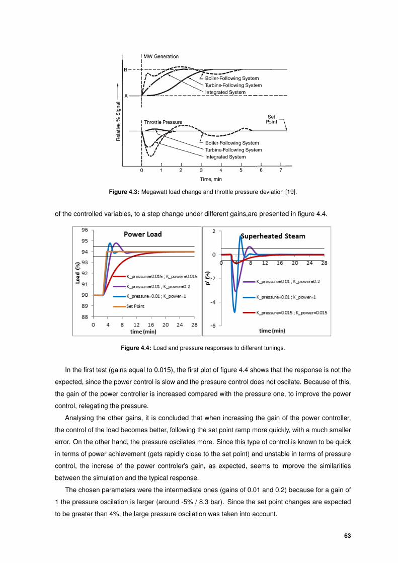
Figure 4.3: Megawatt load change and throttle pressure deviation [19].
of the controlled variables, to a step change under different gains,are presented in figure 4.4.
Figure 4.4: Load and pressure responses to different tunings.
In the first test (gains equal to 0.015), the first plot of figure 4.4 shows that the response is not the
expected, since the power control is slow and the pressure control does not oscilate. Because of this,
the gain of the power controller is increased compared with the pressure one, to improve the power
control, relegating the pressure.
Analysing the other gains, it is concluded that when increasing the gain of the power controller,
the control of the load becomes better, following the set point ramp more quickly, with a much smaller
error. On the other hand, the pressure oscilates more. Since this type of control is known to be quick
in terms of power achievement (gets rapidly close to the set point) and unstable in terms of pressure
control, the increse of the power controler’s gain, as expected, seems to improve the similarities
between the simulation and the typical response.
The chosen parameters were the intermediate ones (gains of 0.01 and 0.2) because for a gain of
1 the pressure oscilation is larger (around -5% / 8.3 bar). Since the set point changes are expected
to be greater than 4%, the large pressure oscilation was taken into account.
63
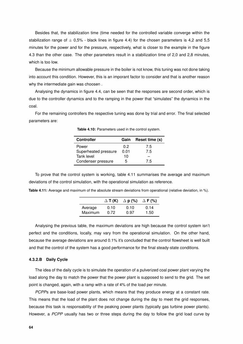
Besides that, the stabilization time (time needed for the controlled variable converge within the
stabilization range of ± 0,5% - black lines in figure 4.4) for the chosen parameters is 4,2 and 5,5
minutes for the power and for the pressure, respectively, what is closer to the example in the figure
4.3 than the other case. The other parameters result in a stabilization time of 2,0 and 2,8 minutes,
which is too low.
Because the minimum allowable pressure in the boiler is not know, this tuning was not done taking
into account this condition. However, this is an imporant factor to consider and that is another reason
why the intermediate gain was choosen .
Analysing the dynamics in figure 4.4, can be seen that the responses are second order, which is
due to the controller dynamics and to the ramping in the power that “simulates” the dynamics in the
coal.
For the remaining controllers the respective tuning was done by trial and error. The final selected
parameters are:
Table 4.10: Parameters used in the control system.
Controller Gain Reset time (s)
Power 0.2 7.5Superheated pressure 0.01 7.5Tank level 10 –Condenser pressure 5 7.5
To prove that the control system is working, table 4.11 summarises the average and maximum
deviations of the control simulation, with the operational simulation as reference.
Table 4.11: Average and maximum of the absolute stream deviations from operational (relative deviation, in %).
∆ T (K) ∆ p (%) ∆ F (%)
Average 0.10 0.10 0.14Maximum 0.72 0.97 1.50
Analysing the previous table, the maximum deviations are high because the control system isn’t
perfect and the conditions, locally, may vary from the operational simulation. On the other hand,
because the average deviations are around 0.1% it’s concluded that the control flowsheet is well built
and that the control of the system has a good performance for the final steady-state conditions.
4.3.2.B Daily Cycle
The idea of the daily cycle is to simulate the operation of a pulverized coal power plant varying the
load along the day to match the power that the power plant is supposed to send to the grid. The set
point is changed, again, with a ramp with a rate of 4% of the load per minute.
PCPPs are base-load power plants, which means that they produce energy at a constant rate.
This means that the load of the plant does not change during the day to meet the grid responses,
because this task is responsability of the peaking power plants (typically gas turbine power plants).
However, a PCPP usually has two or three steps during the day to follow the grid load curve by
64
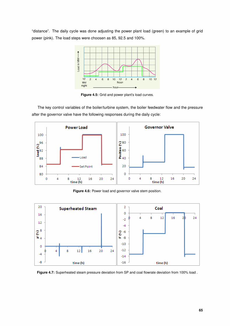
“distance”. The daily cycle was done adjusting the power plant load (green) to an example of grid
power (pink). The load steps were choosen as 85, 92.5 and 100%.
Figure 4.5: Grid and power plant’s load curves.
The key control variables of the boiler/turbine system, the boiler feedwater flow and the pressure
after the governor valve have the following responses during the daily cycle:
Figure 4.6: Power load and governor valve stem position.
Figure 4.7: Superheated steam pressure deviation from SP and coal flowrate deviation from 100% load .
65
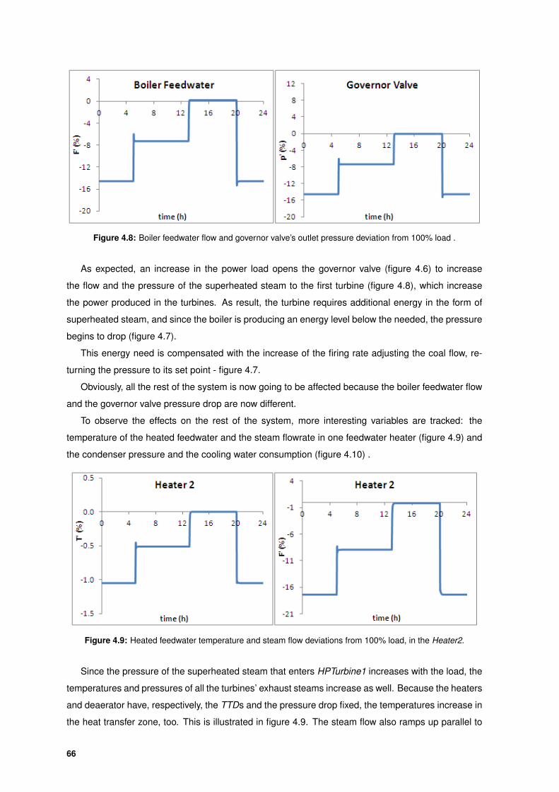
Figure 4.8: Boiler feedwater flow and governor valve’s outlet pressure deviation from 100% load .
As expected, an increase in the power load opens the governor valve (figure 4.6) to increase
the flow and the pressure of the superheated steam to the first turbine (figure 4.8), which increase
the power produced in the turbines. As result, the turbine requires additional energy in the form of
superheated steam, and since the boiler is producing an energy level below the needed, the pressure
begins to drop (figure 4.7).
This energy need is compensated with the increase of the firing rate adjusting the coal flow, re-
turning the pressure to its set point - figure 4.7.
Obviously, all the rest of the system is now going to be affected because the boiler feedwater flow
and the governor valve pressure drop are now different.
To observe the effects on the rest of the system, more interesting variables are tracked: the
temperature of the heated feedwater and the steam flowrate in one feedwater heater (figure 4.9) and
the condenser pressure and the cooling water consumption (figure 4.10) .
Figure 4.9: Heated feedwater temperature and steam flow deviations from 100% load, in the Heater2.
Since the pressure of the superheated steam that enters HPTurbine1 increases with the load, the
temperatures and pressures of all the turbines’ exhaust steams increase as well. Because the heaters
and deaerator have, respectively, the TTDs and the pressure drop fixed, the temperatures increase in
the heat transfer zone, too. This is illustrated in figure 4.9. The steam flow also ramps up parallel to
66
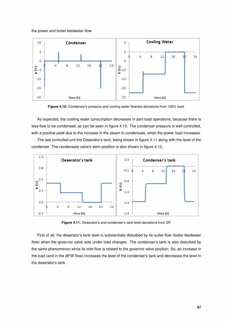
the power and boiler feedwater flow.
Figure 4.10: Condenser’s pressure and cooling water flowrate deviations from 100% load.
As expected, the cooling water consumption decreases in part-load operations, because there is
less flow to be condensed, as can be seen in figure 4.10. The condenser pressure is well controlled,
with a positive peak due to the increase in the steam to condensate, when the power load increases.
The last controlled unit the Deaerator’s tank, being shown in figure 4.11 along with the level of the
condenser. The condensate valve’s stem position is also shown in figure 4.12.
Figure 4.11: Deaerator’s and condenser’s tank level deviations from SP.
First of all, the deaerator’s tank level is substantially disturbed by its outlet flow (boiler feedwater
flow) when the governor valve acts under load changes. The condenser’s tank is also disturbed by
the same phenomenon since its inlet flow is related to the governor valve position. So, an increase in
the load (and in the BFW flow) increases the level of the condenser’s tank and decreases the level in
the deaerator’s tank.
67
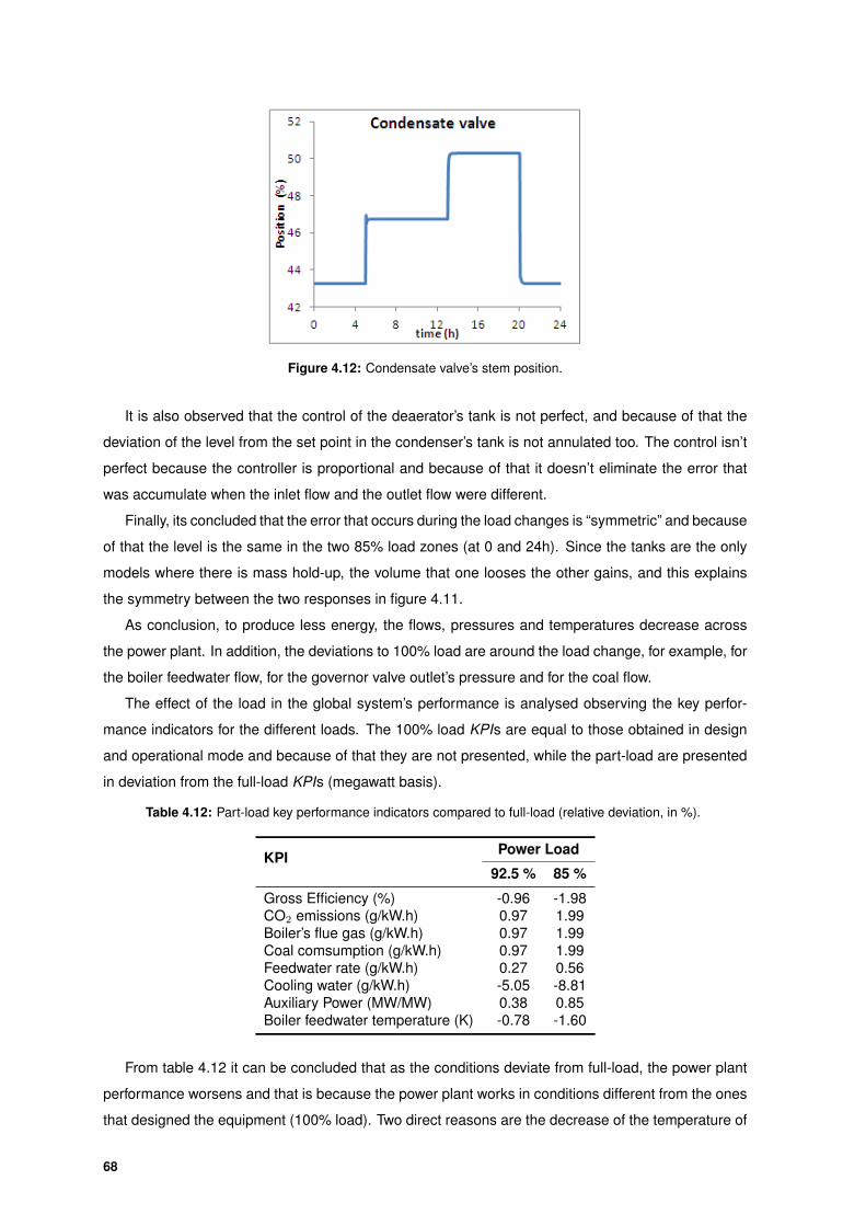
Figure 4.12: Condensate valve’s stem position.
It is also observed that the control of the deaerator’s tank is not perfect, and because of that the
deviation of the level from the set point in the condenser’s tank is not annulated too. The control isn’t
perfect because the controller is proportional and because of that it doesn’t eliminate the error that
was accumulate when the inlet flow and the outlet flow were different.
Finally, its concluded that the error that occurs during the load changes is “symmetric” and because
of that the level is the same in the two 85% load zones (at 0 and 24h). Since the tanks are the only
models where there is mass hold-up, the volume that one looses the other gains, and this explains
the symmetry between the two responses in figure 4.11.
As conclusion, to produce less energy, the flows, pressures and temperatures decrease across
the power plant. In addition, the deviations to 100% load are around the load change, for example, for
the boiler feedwater flow, for the governor valve outlet’s pressure and for the coal flow.
The effect of the load in the global system’s performance is analysed observing the key perfor-
mance indicators for the different loads. The 100% load KPIs are equal to those obtained in design
and operational mode and because of that they are not presented, while the part-load are presented
in deviation from the full-load KPIs (megawatt basis).
Table 4.12: Part-load key performance indicators compared to full-load (relative deviation, in %).
KPI Power Load
92.5 % 85 %
Gross Efficiency (%) -0.96 -1.98CO2 emissions (g/kW.h) 0.97 1.99Boiler’s flue gas (g/kW.h) 0.97 1.99Coal comsumption (g/kW.h) 0.97 1.99Feedwater rate (g/kW.h) 0.27 0.56Cooling water (g/kW.h) -5.05 -8.81Auxiliary Power (MW/MW) 0.38 0.85Boiler feedwater temperature (K) -0.78 -1.60
From table 4.12 it can be concluded that as the conditions deviate from full-load, the power plant
performance worsens and that is because the power plant works in conditions different from the ones
that designed the equipment (100% load). Two direct reasons are the decrease of the temperature of
68
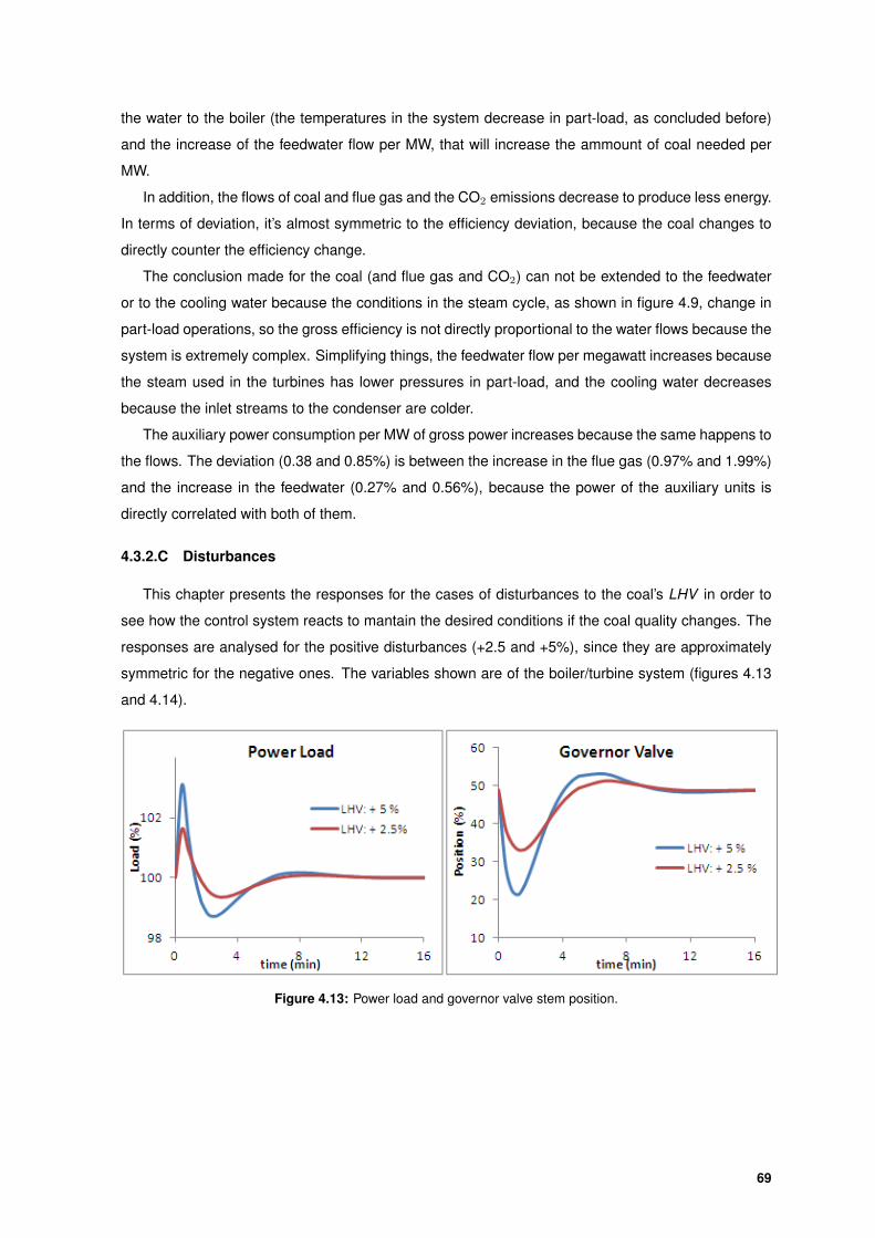
the water to the boiler (the temperatures in the system decrease in part-load, as concluded before)
and the increase of the feedwater flow per MW, that will increase the ammount of coal needed per
MW.
In addition, the flows of coal and flue gas and the CO2 emissions decrease to produce less energy.
In terms of deviation, it’s almost symmetric to the efficiency deviation, because the coal changes to
directly counter the efficiency change.
The conclusion made for the coal (and flue gas and CO2) can not be extended to the feedwater
or to the cooling water because the conditions in the steam cycle, as shown in figure 4.9, change in
part-load operations, so the gross efficiency is not directly proportional to the water flows because the
system is extremely complex. Simplifying things, the feedwater flow per megawatt increases because
the steam used in the turbines has lower pressures in part-load, and the cooling water decreases
because the inlet streams to the condenser are colder.
The auxiliary power consumption per MW of gross power increases because the same happens to
the flows. The deviation (0.38 and 0.85%) is between the increase in the flue gas (0.97% and 1.99%)
and the increase in the feedwater (0.27% and 0.56%), because the power of the auxiliary units is
directly correlated with both of them.
4.3.2.C Disturbances
This chapter presents the responses for the cases of disturbances to the coal’s LHV in order to
see how the control system reacts to mantain the desired conditions if the coal quality changes. The
responses are analysed for the positive disturbances (+2.5 and +5%), since they are approximately
symmetric for the negative ones. The variables shown are of the boiler/turbine system (figures 4.13
and 4.14).
Figure 4.13: Power load and governor valve stem position.
69
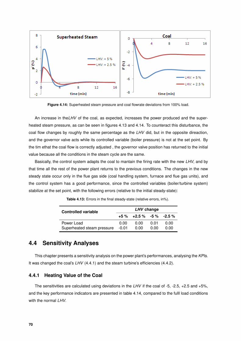
Figure 4.14: Superheated steam pressure and coal flowrate deviations from 100% load.
An increase in theLHV of the coal, as expected, increases the power produced and the super-
heated steam pressure, as can be seen in figures 4.13 and 4.14. To counteract this disturbance, the
coal flow changes by roughly the same percentage as the LHV did, but in the opposite direaction,
and the governor valve acts while its controlled variable (boiler pressure) is not at the set point. By
the tim ethat the coal flow is correctly adjusted , the governor valve position has returned to the initial
value because all the conditions in the steam cycle are the same.
Basically, the control system adapts the coal to mantain the firing rate with the new LHV, and by
that time all the rest of the power plant returns to the previous conditions. The changes in the new
steady state occur only in the flue gas side (coal handling system, furnace and flue gas units), and
the control system has a good performance, since the controlled variables (boiler/turbine system)
stabilize at the set point, with the following errors (relative to the initial steady-state):
Table 4.13: Errors in the final steady-state (relative errors, in%).
Controlled variable LHV change
+5 % +2.5 % -5 % -2.5 %
Power Load 0.00 0.00 0.01 0.00Superheated steam pressure -0.01 0.00 0.00 0.00
4.4 Sensitivity Analyses
This chapter presents a sensitivity analysis on the power plant’s performances, analysing the KPIs.
It was changed the coal’s LHV (4.4.1) and the steam turbine’s efficiencies (4.4.2).
4.4.1 Heating Value of the Coal
The sensitivities are calculated using deviations in the LHV if the coal of -5, -2.5, +2.5 and +5%,
and the key performance indicators are presented in table 4.14, compared to the fulll load conditions
with the normal LHV.
70
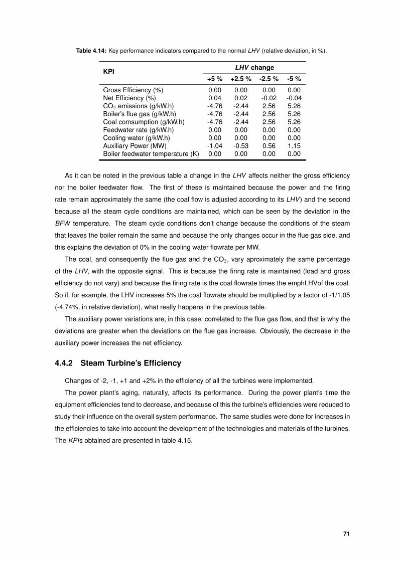
Table 4.14: Key performance indicators compared to the normal LHV (relative deviation, in %).
KPI LHV change
+5 % +2.5 % -2.5 % -5 %
Gross Efficiency (%) 0.00 0.00 0.00 0.00Net Efficiency (%) 0.04 0.02 -0.02 -0.04CO2 emissions (g/kW.h) -4.76 -2.44 2.56 5.26Boiler’s flue gas (g/kW.h) -4.76 -2.44 2.56 5.26Coal comsumption (g/kW.h) -4.76 -2.44 2.56 5.26Feedwater rate (g/kW.h) 0.00 0.00 0.00 0.00Cooling water (g/kW.h) 0.00 0.00 0.00 0.00Auxiliary Power (MW) -1.04 -0.53 0.56 1.15Boiler feedwater temperature (K) 0.00 0.00 0.00 0.00
As it can be noted in the previous table a change in the LHV affects neither the gross efficiency
nor the boiler feedwater flow. The first of these is maintained because the power and the firing
rate remain approximately the same (the coal flow is adjusted according to its LHV ) and the second
because all the steam cycle conditions are maintained, which can be seen by the deviation in the
BFW temperature. The steam cycle conditions don’t change because the conditions of the steam
that leaves the boiler remain the same and because the only changes occur in the flue gas side, and
this explains the deviation of 0% in the cooling water flowrate per MW.
The coal, and consequently the flue gas and the CO2, vary aproximately the same percentage
of the LHV, with the opposite signal. This is because the firing rate is maintained (load and gross
efficiency do not vary) and because the firing rate is the coal flowrate times the emphLHVof the coal.
So if, for example, the LHV increases 5% the coal flowrate should be multiplied by a factor of -1/1.05
(-4,74%, in relative deviation), what really happens in the previous table.
The auxiliary power variations are, in this case, correlated to the flue gas flow, and that is why the
deviations are greater when the deviations on the flue gas increase. Obviously, the decrease in the
auxiliary power increases the net efficiency.
4.4.2 Steam Turbine’s Efficiency
Changes of -2, -1, +1 and +2% in the efficiency of all the turbines were implemented.
The power plant’s aging, naturally, affects its performance. During the power plant’s time the
equipment efficiencies tend to decrease, and because of this the turbine’s efficiencies were reduced to
study their influence on the overall system performance. The same studies were done for increases in
the efficiencies to take into account the development of the technologies and materials of the turbines.
The KPIs obtained are presented in table 4.15.
71
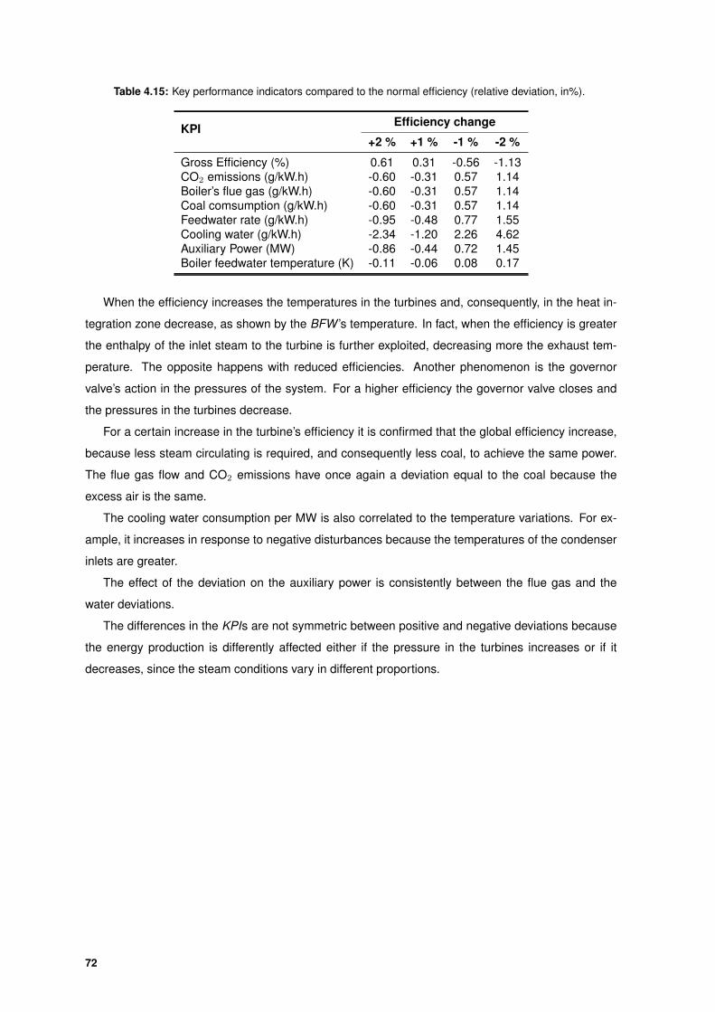
Table 4.15: Key performance indicators compared to the normal efficiency (relative deviation, in%).
KPI Efficiency change
+2 % +1 % -1 % -2 %
Gross Efficiency (%) 0.61 0.31 -0.56 -1.13CO2 emissions (g/kW.h) -0.60 -0.31 0.57 1.14Boiler’s flue gas (g/kW.h) -0.60 -0.31 0.57 1.14Coal comsumption (g/kW.h) -0.60 -0.31 0.57 1.14Feedwater rate (g/kW.h) -0.95 -0.48 0.77 1.55Cooling water (g/kW.h) -2.34 -1.20 2.26 4.62Auxiliary Power (MW) -0.86 -0.44 0.72 1.45Boiler feedwater temperature (K) -0.11 -0.06 0.08 0.17
When the efficiency increases the temperatures in the turbines and, consequently, in the heat in-
tegration zone decrease, as shown by the BFW ’s temperature. In fact, when the efficiency is greater
the enthalpy of the inlet steam to the turbine is further exploited, decreasing more the exhaust tem-
perature. The opposite happens with reduced efficiencies. Another phenomenon is the governor
valve’s action in the pressures of the system. For a higher efficiency the governor valve closes and
the pressures in the turbines decrease.
For a certain increase in the turbine’s efficiency it is confirmed that the global efficiency increase,
because less steam circulating is required, and consequently less coal, to achieve the same power.
The flue gas flow and CO2 emissions have once again a deviation equal to the coal because the
excess air is the same.
The cooling water consumption per MW is also correlated to the temperature variations. For ex-
ample, it increases in response to negative disturbances because the temperatures of the condenser
inlets are greater.
The effect of the deviation on the auxiliary power is consistently between the flue gas and the
water deviations.
The differences in the KPIs are not symmetric between positive and negative deviations because
the energy production is differently affected either if the pressure in the turbines increases or if it
decreases, since the steam conditions vary in different proportions.
72

5Conclusions and Future Work
Contents5.1 Conclusions . . . . . . . . . . . . . . . . . . . . . . . . . . . . . . . . . . . . . . . . 745.2 Future Work . . . . . . . . . . . . . . . . . . . . . . . . . . . . . . . . . . . . . . . . 75
73
5.1 Conclusions
The main objective of this work is to develop a model of a subcritical pulverized coal power plant,
to integrate with all the CCS chain in the future. Dynamic studies were performed to this power plant.
Additionally, the power plant’s performance under different operational conditions was analysed.
The steam cycle and the flue gas side are based on information obtained from the literature [7] [8],
and the gCCS current library is used to build the compound model that represents the power plant.
As additional work, some models that were missing were developed and added to the library.
For full-load operations, the simulated power plant has a gross power output of 769.9 MW, resulting
in a net power of 742.8 MW. Using a subcritical boiler with a typical efficiency of 88.1% [8], the gross
efficiency obtained was 39.6 %. There are no data in the literature for the gross efficiency of the
modelled power plant, but the value is in the typical range (38-40%). The boiler feedwater flow is
2839.8g/kWh.
In terms of the flue gas side, the power plant emits 828.25 g CO2 /kW.h to the atmosphere, a
typical value without capture. This flue gas sent to the stack has a concentration of 20 mg/Nm3 of
ash and 200 mg/Nm3 of SO2 and has no NOx, since the furnace does not produce NOx in the boiler
model. The flue gas emisson is 3870.6 g /kW.h and the coal consumption is 357.3 g /kW.h. The
deviations from the data reported in the literature (Allstrom) are -2.4, -1.5 and -2.0% for the CO2, flue
gas and coal, respectively. Both the flue gas and CO2 emissions and coal consumption are less than
the example used from the literature, because the efficiency is greater, which reduces the material
used per MW.
It is concluded that for part-load conditions the gross efficiency decreases, which indicates that
a pulverized coal power plant should work on the maximum load whenever possible. The gross ef-
ficiency is 39.2 and 38.8% for 92.2 and 85 % load, respectively, and the specific CO2 emissions
increased 1 and 2% (relative to 100% load) to 836.3 and 844.7 g/kWh. The coal consumption in-
creased to 360.8 and 364.5 g/kWh and the flue gas emissions to 3908.1 and 3947.8 g/kWh, the same
relative percentage than for the coal, because the CO2 is direcly correlated with the coal and flue
gas, since the flue gas composition is constant. This efficiency penalty is due to the boiler feedwater
temperature decrease, which increases the coal needed per MW.
For a coal with higher LHV, the gross efficiency is not affected, because the same firing rate is
needed per gross power. In terms of net efficiency, the “real” efficiency to consider from the optimiza-
tion point of view, a coal with a higher LHV improves the power plant, because the coal and flue gas
quantities to handle, and consequently the auxiliary power, are lower. For an increase of 2.5 and 5%
in the LHV, the flue gas (and CO2 emissions) and the coal consumption decrease 2.4 and 4.8%, ,
respectively.
On the other hand, upgrading the steam turbine’s efficiencies increases both the gross and the
net efficiency, because the resources in the steam cycle and in the flue gas side are lower to produce
the same energy.
For example, for an efficiency increase of 2% in the turbines, the gross efficiency increases 0.6%,
74
and for a decrease of 2% the penalty is around 1.1%. For the net efficiency, the advantage of a
turbine system with higher efficiency will be greater because it accounts for the energy savings in
all the auxiliary units. In fact, in the flue gas side the emissions change by -0.6 and +1.1% for each
case, and in the steam cycle the boiler feedwater varies -1.0 and +1.6. It is also concluded that the
improvement (for +2%) is lower than the penalty (for -2%) because the temperatures and pressures
in the system vary differently with the turbine efficiencies.
The sensitivity analyses show that the power plant performance is upgraded using a coal with
higher LHV and with more efficient turbines. However, only an optimization study can answer whether
the performance increase by the coal and turbinesis eventually beneficial, because there are some
implications such as:
• The coal flow per MW is lower but its cost increases with the LHV.
• The investment in the steam turbines increases with increasing turbine efficiency.
• The lower flows in the system decrease the units size and, consequently, the power plant cost.
In terms of control, it’s concluded that changing the load at a rate of 4% per minute, the control ap-
plied to the models has a similar performance when compared to the literature, with quick responses
and small errors.
One limitation of the work is the accuracy of the auxiliary power, and that’s why no values of net
efficiencies are provided in the conclusions.
Since the library models were all steady-state models, the control study is not reliable enought to
draw strong conclusions.From the control point of view this is the main limitation. For example, the
coal dynamics should be appplied because it has very slow dynamics, due to the fuel pulverization in
the mill.
These two limitations could be improved in future work.
5.2 Future Work
There are some details to be taken into account in order to improve the work done in the scope of
this thesis.
Since the gCCS project is at an early stage, the library used to develop the PCPP is in its first
version. Because of this, several issues could be changed in the models, so as to improve the final
conclusions. Actually, a lot of effort and time was spent testing the newly finished models and ensuring
they work together, and because of that some simplifications were made to the models.
As already concluded, the main issue in terms of control is the implementation of dynamics in
some models to improve the reliability of the dynamic responses, and to allow to be used all the
controls and operations that are practiced in the real power plant.
As an example, the implementation of dynamics in the deaerator and in the feedwater heater
would calculate the pressure according to the mass and energy hold-up in the equipment. The hold-
75
up would allow to control the level of these units, and the pressure would enable the equipment to
operate in “pressure-driven” mode, like in the real power plant.
On the other hand, boiler and coal handling units dynamics would also be an important step. This
improvement would allow to analyse the different boiler/turbine system control modes correctly, since
the main difference between them is the fast or slow use of the stored energy and mass in the steam
drum.
Another important improvement would be the insertion of leakage in the steam cycle to turn it into
an open cycle with make-up control.
The models could also be, in general, more detailed to improve the accuracy of the results. As
examples, the feedwater heater should take in account the different zones of heat exchange and
calculate accurately the overall heat transfer coefficient, and the deaerator should be modeled taking
into account the three Rdifferent zones that compose it. The boiler’s furnace should produce NOx
during the combustion, to be removed in the SCR, and to take in account the power consumption of
this removal.
Another important issue is the modelling of other units that would improve both the control and the
power plant performance studies. For example, the modelling of the cooling water and coal systems
would improve the veracity of the auxiliary power calculation to study the power plant’s performance
more accurately, while the modelling of the attemperators in the boiler model would permit control of
both the RH and the SH temperatures.
Connecting the entire CCS chain would be the perfect final step, sending the flue gas to the
capture plant to remove the CO2 before being set to the stack. With this tool, it would be possible to
study the performance of the power plant with capture, and to control all the CCS components.
An optimization of the power plant would be also an interesting work to be done in the future, when
the models allow sizing the most relevant units.
76
Bibliography
[1] F. Birol, “Power to the people: The world outlook for
electricity investment,” International Atomic Energy Agency,
http://www.iaea.org/Publications/Magazines/Bulletin/Bull461/power to the people.html, last
acess in: 17th June 2012.
[2] “Kyoto Protocol to the United Nations Framework convention on climate change,” United Nations,
1998, http://unfccc.inl, last acess in: 20th June 2012.
[3] “Government pledges to cut carbon emissions by 80% by 2050,” The guardian, October 2008,
http://www.guardian.co.uk, last acess in: 15th June 2012.
[4] “World’s Power Plant Emissions Detailed,” The Washington Post, November 2007,
http://www.washingtonpost.com, last acess in: 21st June 2012.
[5] “CO2 Capture Technologies, article 3, alinea 1,” Global CCS Institute, January 2012.
[6] N. Tanaka and R. Wicks, “Power Generation from Coal - Measuring and Reporting Efficiency
Performance and CO2 emissions,” Internation Energy Agency, 2010, http://www.iea.org, last
acess in: 20th June 2012.
[7] L. F. Drbal, P. G. Boston, and K. L. Westra, “Power Plant Engineering,” Kluwer Academic Pub-
lishers, p. 282, December 1995.
[8] C. Bozzuto, N. Nsakala, G. Liljedahl, M. Palkes, and J. Marion, “Engineering feasibility and eco-
nomics of CO2 capture on an existing coal-fired power plant,” June 2011.
[9] J. M. Klara, “Bituminous Coal and Natural Gas to Electricity Final Report,” May 2007.
[10] S. Meinke, F. Gottelt, M. Muller, and E. Hassel, “Modeling of Coal-Fired
Power Units with ThermoPower Focusing on Start-Up Process,” March 2011,
http://www.ep.liu.se/ecp/063/039/ecp11063039.pdf, last acess in 10th September 2012.
[11] R. D. Paranjape, “Modeling and Control of Supercritical Coal Fired Boiler,” May 1996,
http://www.scribd.com/doc/88831036/31295009804930, last acess in 27th August 2012.
[12] A. K. Raja, A. P. Srivastava, and M. Dwivedi, “Power Plant Engineering,” New Age International
Publishers, 2006.
77
[13] T. Riordan, “New Generation Strategy Ultra-Supercritical Technology,” American Electric Power,
November 2006, http://www.asiapacificpartnership.org, last acess in: 21st June 2012.
[14] P. Lako, “Coal-fired power technologies,” ECN, October 2004, http://www.ecn.nl, last acess in:
22nd July 2012.
[15] J. Beer, “Higher Efficiency Power Generation Reduces Emissions,” National Coal Council Issue
Paper, 2009, http://web.mit.edu/mitei/docs/reports/beer-emissions.pdf, last acess in: 22nd July
2012.
[16] M. Romeo, S. Espatorelo, and I. Bolea, “Designing a supercritical steam cycle to integrate the
energy requirements of co2 amine scrubbing. volume 2, issue 4, pages 563-570,” International
Journal of Greenhouse Gas Control, October 2008.
[17] T. Ghosh and M. Prelas, “Energy resources and systems: Volume 1: Fundamentals and non-
renewable resources,” Springer Science + Business Media , 2009, http://www.scribd.com, last
acess in: 22nd July 2012.
[18] M. Boyce, “Handbook for cogeneration and combined cycle power plants,” American Society of
Mechanical Engineers, 2002, http://books.google.co.uk/books/, last acess in: 23rd July 2012.
[19] S. Wilcox, “Steam, its generation and use - 41st ed,” The Babcock Wilcox Company, 2005.
[20] A. Bhatia, “Improving energy efficiency of boyler systems,” Continuing Education and Devel-
opment, Inc., https://www.cedengineering.com/upload/Energy%20Efficiency%20Boilers.pdf, last
acess in: 25th July 2012.
[21] “The formation of nox,” http://www.alentecinc.com, last acess in: 25th July 2012.
[22] “Thermodynamics and heat transfer. the secondary loop: A thermodynamic cycle. chapter 3.”
http://www.scribd.com, last acess in: 25th July 2012.
[23] L. F. Drbal, P. G. Boston, and K. L. Westra, “Power Plant Engineering,” Kluwer Academic Pub-
lishers, December 1995, http://books.google.pt/books, last acess in: 25th July 2012.
[24] D. Hasler, W. Rosequist, and R. Gaikwad, “Coal-Fired Power Plant Heat rate reductions,” Sargent
& Lundy, LLC, January 2009, http://books.google.pt/books, last acess in: 25th July 2012.
[25] “Basics of closed feedwater heaters,” Heat Exchange Institute, December 2007,
http://www.heatexchange.org, last acess in: 11th July 2012.
[26] “Power Generation Process Basics,” http://www.scribd.com/doc/18237621/Power-Plant-Basics:
14th June 2012.
[27] “Basic Principle Of Deaerator and Deaeration,” Mechanical Engineering 4 U, October 2011,
http://www.mechanicalengineering4u.com, last acess in: 4th June 2012.
78
[28] McCabe, Smith, and Harriott, “Unit Operations of Chemical Engineering 6th ed,” McGraw-Hill
International Edition, October 2001.
[29] D. Mussatti, “EPA Air Pollution Control Cost Manual - 6th ed,” EPA, January 2002.
[30] I. Nova, C. Ciardellia, and E. Tronconi, “NO/NO2-NH3 SCR reaction over
a V-based catalyst for Diesel exhaust after treatment,” Politecnico di Milano,
http://www.nacatsoc.org20nam/abstractsO-S4-32.pdf, last acess in: 20th July 2012.
[31] C. Branan, “Rules of Thumb for Chemical Esngineers, page 231,” GPP, 2005,
http://books.google.pt/books, last acess in: 24th July 2012.
[32] K. Krishnaswamy and M. P. Bala, “Power Plant Instrumentation,” PHI, 2011,
http://books.google.pt/books, last acess in: 25th August 2012.
[33] D. Lindsley, “Power-plant control and instrumentation,” The Institution of Electrical Engineers,
2000, http://books.google.pt/books, last acess in: 25th August 2012.
[34] “Main Steam Supply and Feedwater System,” January 1996,
https://canteach.candu.org/Content20Library/19930205.pdf, last acess in: 28th June 2012.
[35] V. Jovel, “Instrumentation appraisal in single and double flash power plants,” United Nations
University, 2011, http://www.os.is/gogn/unu-gtp-report/UNU-GTP-2011-07.pdf, last acess in 21st
August 2012.
[36] D. Hite, “Heat rate and feedwater heater level control,” Magnetrol International & Orion Instru-
ments, 2010, http://mx.magnetrol.com/pdfs/1/41-281.pdf, last acess in: 25th June 2012.
[37] K. Hambrice, “Power Plant Feedwater Heater Level Control,” Pumps & Systems, September
2007, http://www.pump-zone.co, last acess in: 25th June 2012.
[38] “Carbon Capture,” Neural Energy, April 2012, http://www.neuralenergy.info/2011/09/carbon-
capture.html, last acess in: 7th June 2012.
[39] “Carbon Capture and Storage,” KBR, http://www.kbr.com, last acess in: 5th June 2012.
[40] “CO2 Capture, Transport and Storage,” Parliamentary Office of Science and Technology, June
2009, http://www.parliament.uk/documents/post/postpn335.pdf, last acess in 21st June 2012.
[41] “Post Combustion Carbon Capture,” KBR, http://www.kbr.com, last acess in 14th June 2012.
[42] D. F. Cziesla, D. J. Bewerunge, and A. Senzel, “Lunen - State of the Art. Ultra Supercritical Steam
Power Plant Under Construction,” May 2009, http://www.energy.siemens.com/co/pool/hq/power-
generation/power-plants/steam-power-plant-solutions/coal-fired-power-plants/Luenen.pdf, last
acess in 29th August 2012.
79

[43] N. Lusica, T. Xie, , and Y. Lu, “Technology Status and Project Development Risks of Ad-
vanced Coal Power Generation Technologies in APEC Developing Economies,” October 2008,
http://www.egcfe.ewg.apec.org/projects/EWG 06-2007 Report20 2008-10-01.pdf, last acess in
29th August 2012.
80

AgCCS Model Library
A-1
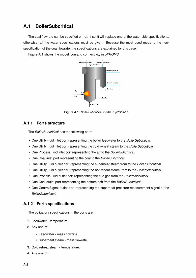
A.1 BoilerSubcritical
The coal flowrate can be specified or not. If so, it will replace one of the water side specifications,
otherwise, all the water specifications must be given. Because the most used mode is the non-
specification of the coal flowrate, the specifications are explained for this case.
Figure A.1 shows the model icon and connectivity in gPROMS.
Figure A.1: BoilerSubcritical model in gPROMS.
A.1.1 Ports structure
The BoilerSubcritical has the following ports:
• One UtilityFluid inlet port representing the boiler feedwater to the BoilerSubcritical.
• One UtilityFluid inlet port representing the cold reheat steam to the BoilerSubcritical.
• One ProcessFluid inlet port representing the air to the BoilerSubcritical.
• One Coal inlet port representing the coal to the BoilerSubcritical.
• One UtilityFluid outlet port representing the superheat steam from to the BoilerSubcritical.
• One UtilityFluid outlet port representing the hot reheat steam from to the BoilerSubcritical.
• One ProcessFluid outlet port representing the flue gas from the BoilerSubcritical.
• One Coal outlet port representing the bottom ash from the BoilerSubcritical.
• One ControlSignal outlet port representing the superheat pressure measurement signal of the
BoilerSubcritical.
A.1.2 Ports specifications
The obligatory specifications in the ports are:
1. Feedwater - temperature.
2. Any one of:
• Feedwater - mass flowrate.
• Superheat steam - mass flowrate.
3. Cold reheat steam - temperature.
4. Any one of:
A-2
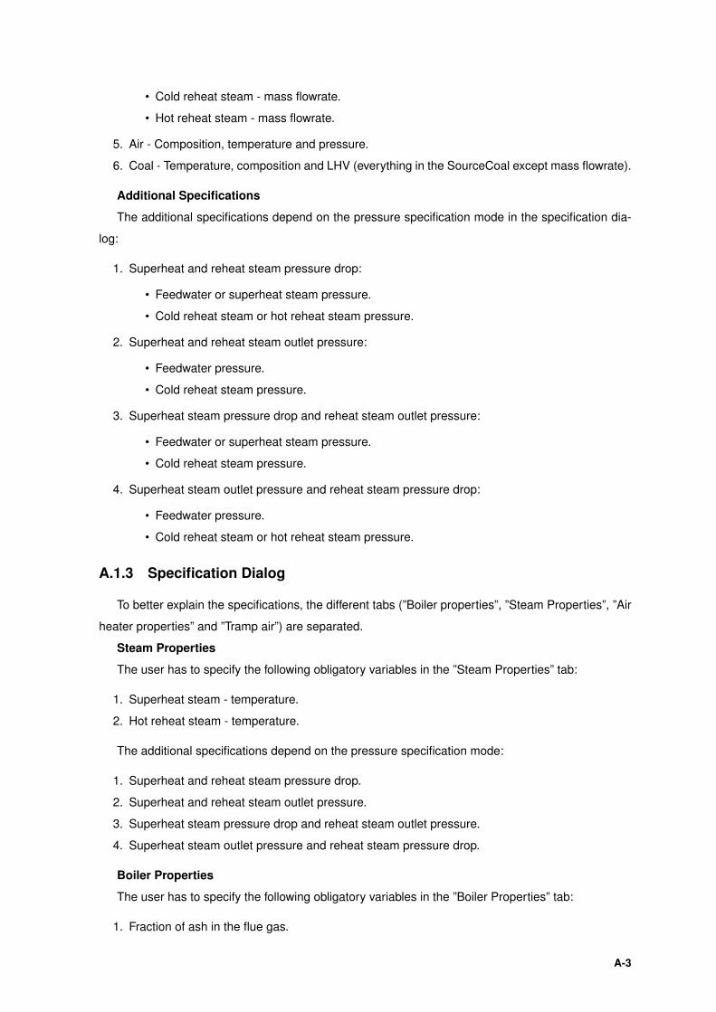
• Cold reheat steam - mass flowrate.
• Hot reheat steam - mass flowrate.
5. Air - Composition, temperature and pressure.
6. Coal - Temperature, composition and LHV (everything in the SourceCoal except mass flowrate).
Additional Specifications
The additional specifications depend on the pressure specification mode in the specification dia-
log:
1. Superheat and reheat steam pressure drop:
• Feedwater or superheat steam pressure.
• Cold reheat steam or hot reheat steam pressure.
2. Superheat and reheat steam outlet pressure:
• Feedwater pressure.
• Cold reheat steam pressure.
3. Superheat steam pressure drop and reheat steam outlet pressure:
• Feedwater or superheat steam pressure.
• Cold reheat steam pressure.
4. Superheat steam outlet pressure and reheat steam pressure drop:
• Feedwater pressure.
• Cold reheat steam or hot reheat steam pressure.
A.1.3 Specification Dialog
To better explain the specifications, the different tabs (”Boiler properties”, ”Steam Properties”, ”Air
heater properties” and ”Tramp air”) are separated.
Steam Properties
The user has to specify the following obligatory variables in the ”Steam Properties” tab:
1. Superheat steam - temperature.
2. Hot reheat steam - temperature.
The additional specifications depend on the pressure specification mode:
1. Superheat and reheat steam pressure drop.
2. Superheat and reheat steam outlet pressure.
3. Superheat steam pressure drop and reheat steam outlet pressure.
4. Superheat steam outlet pressure and reheat steam pressure drop.
Boiler Properties
The user has to specify the following obligatory variables in the ”Boiler Properties” tab:
1. Fraction of ash in the flue gas.
A-3
2. Fraction of carbon in the ash.
3. Pressure of the flue gas.
4. Temperature of the bottom ash.
5. Efficiency of the Boiler.
6. Any one of:
• Mass fraction of oxygen in the flue gas.
• Molar fraction of oxygen in dry flue gas.
• Excess of air.
Air heater properties
If the user chooses the have air heater in the boiler the following obligatory variables have to be
specified in the ”Air heater properties” tab:
1. Flue gas pressure drop.
2. Air pressure drop.
3. Air heater leakage fraction.
4. Air heater heat transfer efficiency.
5. Any one of:
• Heat exchanger effectiveness.
• Flue gas inlet temperature.
• Air outlet temperature.
Tramp air
The user has to specify the following obligatory variable in the ”Tramp air” tab:
1. Inlet tramp air fraction.
2. Tramp air temperature
3. Tramp air pressure.
A.2 GovernorValve
Figure A.2 shows the model icon and connectivity in gPROMS.
Figure A.2: GovernorValve model in gPROMS.
A-4
A.2.1 Ports structure
The GovernorValve has the following ports:
• One UtilityFluid inlet port representing the superheat steam inlet to the GovernorValve.
• One ControlSignal inlet port representing the stem position signal to the GovernorValve.
• One UtilityFluid outlet port representing the superheat steam outlet from the GovernorValve.
A.2.2 Ports specifications
The obligatory specifications in the ports are:
1. Inlet superheat steam - temperature.
2. Any one of:
• Inlet superheat steam - pressure.
• Outlet superheat steam - pressure.
Additional Specifications
1. Pressure drop known:
• Stem position specified:
– Inlet or outlet superheat steam - pressure.
• Stem position controlled:
– Inlet or outlet superheat steam - pressure.
– Inlet signal - stem position.
2. Specify flow coefficient:
• Stem position specified:
– – .
• Stem position controlled:
– Inlet signal - stem position.
The additional specifications depend on the pressure specification mode in the specification dia-
log:
A.2.3 Specification Dialog
The user has to specify the following obligatory variables in the specification dialog:
1. Inherent characteristic.
Additional specifications
The additional specifications depend on the mode:
1. Pressure drop known:
A-5
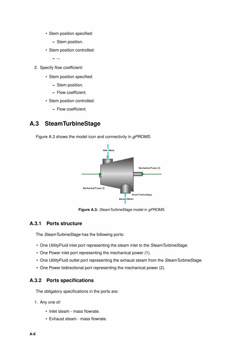
• Stem position specified:
– Stem position.
• Stem position controlled:
– –.
2. Specify flow coefficient:
• Stem position specified:
– Stem position.
– Flow coefficient.
• Stem position controlled:
– Flow coefficient.
A.3 SteamTurbineStage
Figure A.3 shows the model icon and connectivity in gPROMS.
Figure A.3: SteamTurbineStage model in gPROMS.
A.3.1 Ports structure
The SteamTurbineStage has the following ports:
• One UtilityFluid inlet port representing the steam inlet to the SteamTurbineStage.
• One Power inlet port representing the mechanical power (1).
• One UtilityFluid outlet port representing the exhaust steam from the SteamTurbineStage.
• One Power bidirectional port representing the mechanical power (2).
A.3.2 Ports specifications
The obligatory specifications in the ports are:
1. Any one of:
• Inlet steam - mass flowrate.
• Exhaust steam - mass flowrate.
A-6
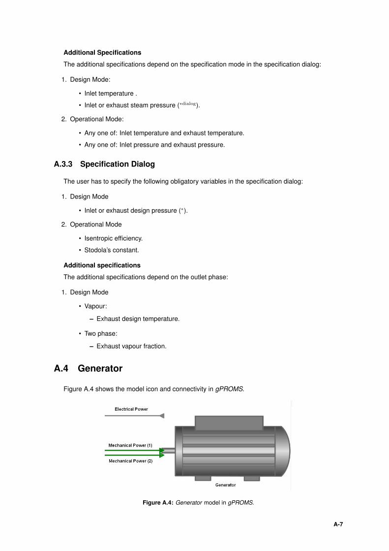
Additional Specifications
The additional specifications depend on the specification mode in the specification dialog:
1. Design Mode:
• Inlet temperature .
• Inlet or exhaust steam pressure (∗dialog).
2. Operational Mode:
• Any one of: Inlet temperature and exhaust temperature.
• Any one of: Inlet pressure and exhaust pressure.
A.3.3 Specification Dialog
The user has to specify the following obligatory variables in the specification dialog:
1. Design Mode
• Inlet or exhaust design pressure (∗).
2. Operational Mode
• Isentropic efficiency.
• Stodola’s constant.
Additional specifications
The additional specifications depend on the outlet phase:
1. Design Mode
• Vapour:
– Exhaust design temperature.
• Two phase:
– Exhaust vapour fraction.
A.4 Generator
Figure A.4 shows the model icon and connectivity in gPROMS.
Figure A.4: Generator model in gPROMS.
A-7
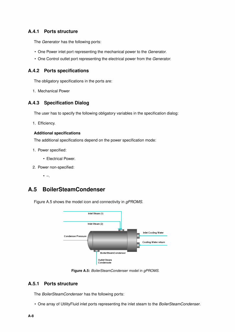
A.4.1 Ports structure
The Generator has the following ports:
• One Power inlet port representing the mechanical power to the Generator.
• One Control outlet port representing the electrical power from the Generator.
A.4.2 Ports specifications
The obligatory specifications in the ports are:
1. Mechanical Power
A.4.3 Specification Dialog
The user has to specify the following obligatory variables in the specification dialog:
1. Efficiency.
Additional specifications
The additional specifications depend on the power specification mode:
1. Power specified:
• Electrical Power.
2. Power non-specified:
• –.
A.5 BoilerSteamCondenser
Figure A.5 shows the model icon and connectivity in gPROMS.
Figure A.5: BoilerSteamCondenser model in gPROMS.
A.5.1 Ports structure
The BoilerSteamCondenser has the following ports:
• One array of UtilityFluid inlet ports representing the inlet steam to the BoilerSteamCondenser.
A-8
• One UtilityFluid inlet port representing the inlet cooling water to the BoilerSteamCondenser.
• One UtilityFluid outlet port representing the outlet steam condensate from the BoilerSteamCon-
denser.
• One UtilityFluid outlet port representing the cooling water return from the BoilerSteamCon-
denser.
• One Control outlet port representing the pressure measurement of the BoilerSteamCondenser.
A.5.2 Ports specifications
The obligatory specifications in the ports are:
1. Inlet Steam(s): Temperature, pressure and mass flowrate.
2. Inlet Cooling water: Temperature and pressure. Mass flowrate (∗dialog).
A.5.3 Specification Dialog
The user has to specify the following obligatory variables in the specification dialog:
1. Overall heat transfer coefficient.
2. Cooling water pressure drop.
Additional specifications
The additional specifications depend on the specification mode:
1. Condenser pressure:
• Design Mode:
– Condenser pressure.
– Any one of: Cooling water return temperature and minimum temperature difference.
• Operational Mode:
– Heat transfer area.
– Any one of: Condenser pressure, cooling water return temperature and minimum tem-
perature difference.
2. Cooling water flow known (∗):
• Design Mode:
– Condenser pressure.
• Operational Mode:
– Heat transfer area.
A.6 FeedWaterHeater
Figure A.6 shows the model icon and connectivity in gPROMS.
A-9
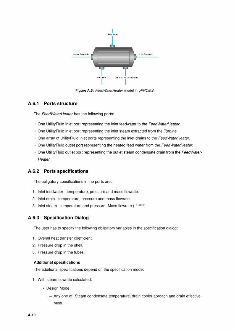
Figure A.6: FeedWaterHeater model in gPROMS.
A.6.1 Ports structure
The FeedWaterHeater has the following ports:
• One UtilityFluid inlet port representing the inlet feedwater to the FeedWaterHeater.
• One UtilityFluid inlet port representing the inlet steam extracted from the Turbine.
• One array of UtilityFluid inlet ports representing the inlet drains to the FeedWaterHeater.
• One UtilityFluid outlet port representing the heated feed water from the FeedWaterHeater.
• One UtilityFluid outlet port representing the outlet steam condensate drain from the FeedWater-
Heater.
A.6.2 Ports specifications
The obligatory specifications in the ports are:
1. Inlet feedwater - temperature, pressure and mass flowrate.
2. Inlet drain - temperature, pressure and mass flowrate.
3. Inlet steam - temperature and pressure. Mass flowrate (∗dialog).
A.6.3 Specification Dialog
The user has to specify the following obligatory variables in the specification dialog:
1. Overall heat transfer coefficient.
2. Pressure drop in the shell.
3. Pressure drop in the tubes.
Additional specifications
The additional specifications depend on the specification mode:
1. With steam flowrate calculated:
• Design Mode:
– Any one of: Steam condensate temperature, drain cooler aproach and drain effective-
ness.
A-10
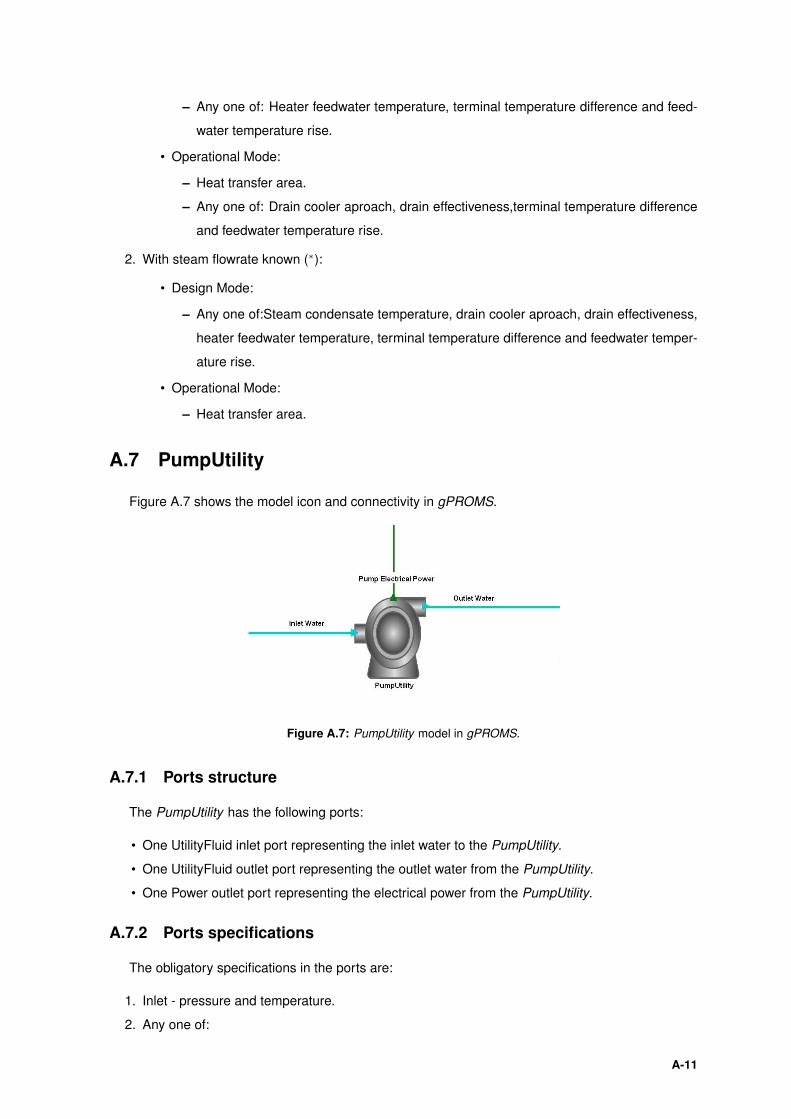
– Any one of: Heater feedwater temperature, terminal temperature difference and feed-
water temperature rise.
• Operational Mode:
– Heat transfer area.
– Any one of: Drain cooler aproach, drain effectiveness,terminal temperature difference
and feedwater temperature rise.
2. With steam flowrate known (∗):
• Design Mode:
– Any one of:Steam condensate temperature, drain cooler aproach, drain effectiveness,
heater feedwater temperature, terminal temperature difference and feedwater temper-
ature rise.
• Operational Mode:
– Heat transfer area.
A.7 PumpUtility
Figure A.7 shows the model icon and connectivity in gPROMS.
Figure A.7: PumpUtility model in gPROMS.
A.7.1 Ports structure
The PumpUtility has the following ports:
• One UtilityFluid inlet port representing the inlet water to the PumpUtility.
• One UtilityFluid outlet port representing the outlet water from the PumpUtility.
• One Power outlet port representing the electrical power from the PumpUtility.
A.7.2 Ports specifications
The obligatory specifications in the ports are:
1. Inlet - pressure and temperature.
2. Any one of:
A-11
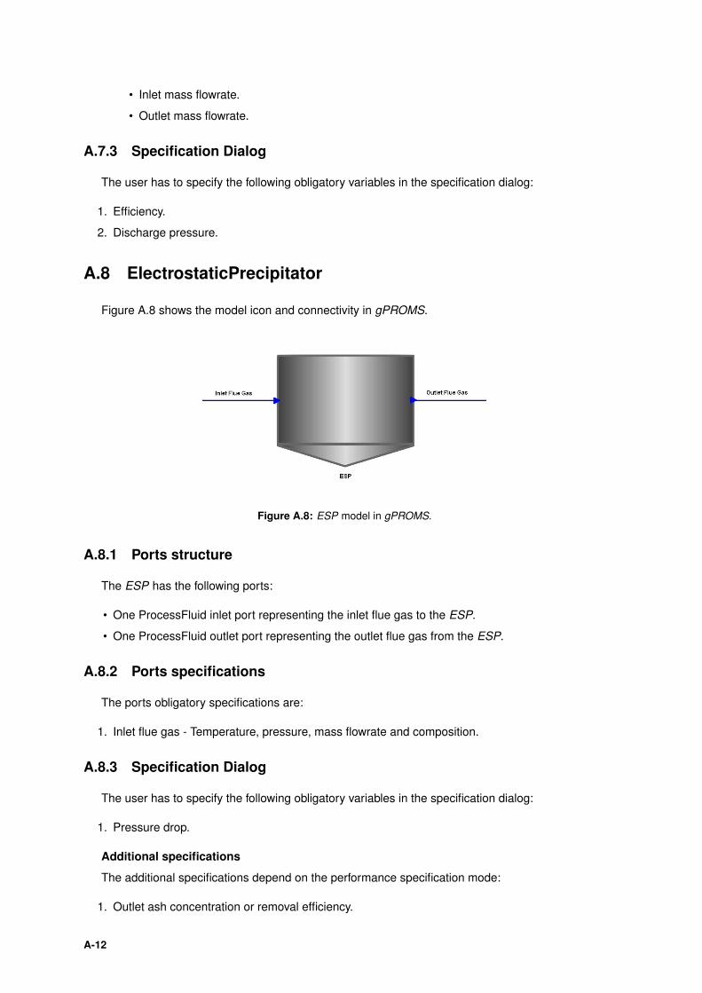
• Inlet mass flowrate.
• Outlet mass flowrate.
A.7.3 Specification Dialog
The user has to specify the following obligatory variables in the specification dialog:
1. Efficiency.
2. Discharge pressure.
A.8 ElectrostaticPrecipitator
Figure A.8 shows the model icon and connectivity in gPROMS.
Figure A.8: ESP model in gPROMS.
A.8.1 Ports structure
The ESP has the following ports:
• One ProcessFluid inlet port representing the inlet flue gas to the ESP.
• One ProcessFluid outlet port representing the outlet flue gas from the ESP.
A.8.2 Ports specifications
The ports obligatory specifications are:
1. Inlet flue gas - Temperature, pressure, mass flowrate and composition.
A.8.3 Specification Dialog
The user has to specify the following obligatory variables in the specification dialog:
1. Pressure drop.
Additional specifications
The additional specifications depend on the performance specification mode:
1. Outlet ash concentration or removal efficiency.
A-12
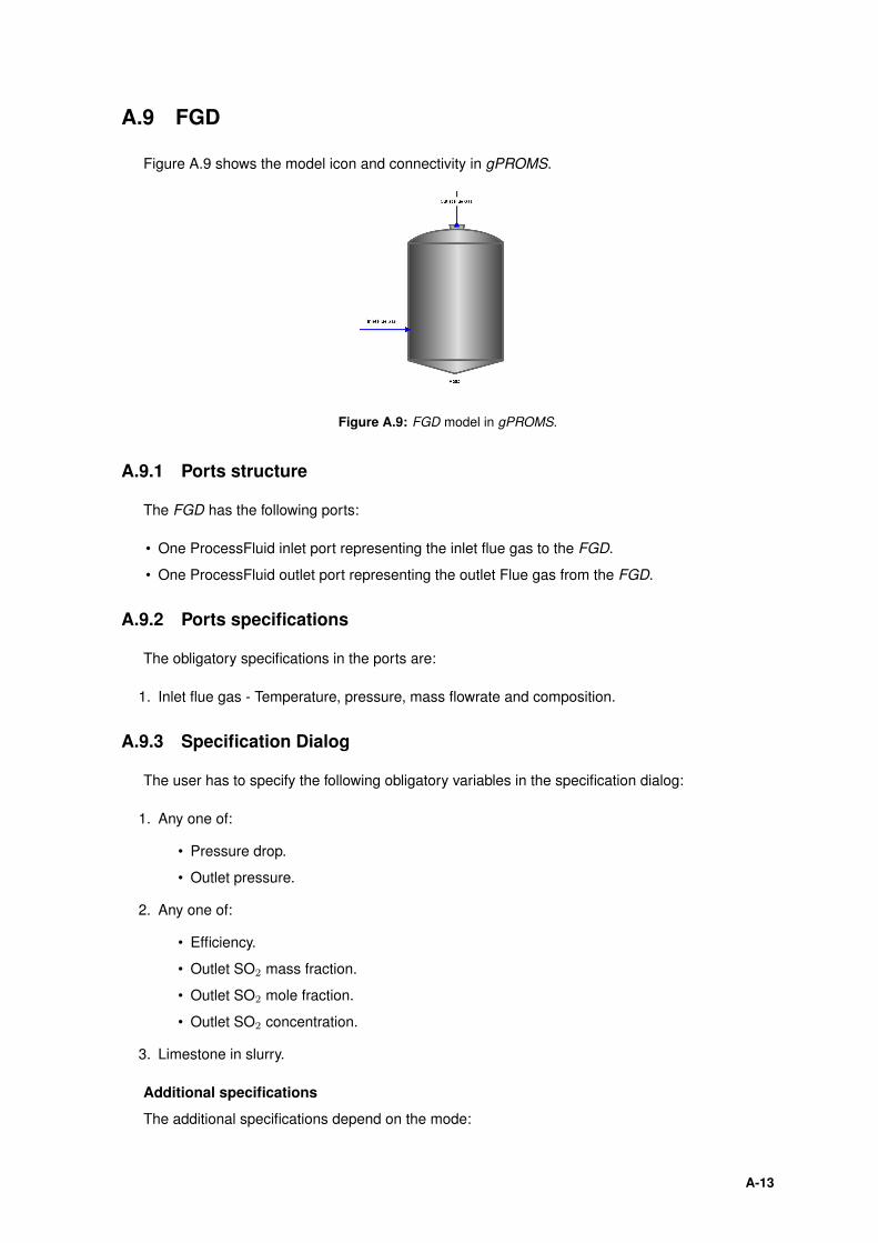
A.9 FGD
Figure A.9 shows the model icon and connectivity in gPROMS.
Figure A.9: FGD model in gPROMS.
A.9.1 Ports structure
The FGD has the following ports:
• One ProcessFluid inlet port representing the inlet flue gas to the FGD.
• One ProcessFluid outlet port representing the outlet Flue gas from the FGD.
A.9.2 Ports specifications
The obligatory specifications in the ports are:
1. Inlet flue gas - Temperature, pressure, mass flowrate and composition.
A.9.3 Specification Dialog
The user has to specify the following obligatory variables in the specification dialog:
1. Any one of:
• Pressure drop.
• Outlet pressure.
2. Any one of:
• Efficiency.
• Outlet SO2 mass fraction.
• Outlet SO2 mole fraction.
• Outlet SO2 concentration.
3. Limestone in slurry.
Additional specifications
The additional specifications depend on the mode:
A-13
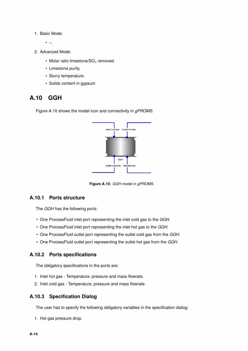
1. Basic Mode:
• –.
2. Advanced Mode:
• Molar ratio limestone/SO2 removed.
• Limestone purity.
• Slurry temperature.
• Solids content in gypsum
A.10 GGH
Figure A.10 shows the model icon and connectivity in gPROMS.
Figure A.10: GGH model in gPROMS.
A.10.1 Ports structure
The GGH has the following ports:
• One ProcessFluid inlet port representing the inlet cold gas to the GGH.
• One ProcessFluid inlet port representing the inlet hot gas to the GGH.
• One ProcessFluid outlet port representing the outlet cold gas from the GGH.
• One ProcessFluid outlet port representing the outlet hot gas from the GGH.
A.10.2 Ports specifications
The obligatory specifications in the ports are:
1. Inlet hot gas - Temperature, pressure and mass flowrate.
2. Inlet cold gas - Temperature, pressure and mass flowrate.
A.10.3 Specification Dialog
The user has to specify the following obligatory variables in the specification dialog:
1. Hot gas pressure drop.
A-14
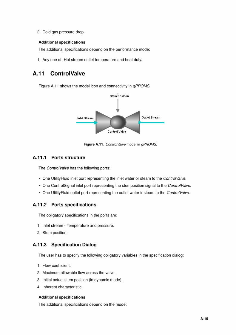
2. Cold gas pressure drop.
Additional specifications
The additional specifications depend on the performance mode:
1. Any one of: Hot stream outlet temperature and heat duty.
A.11 ControlValve
Figure A.11 shows the model icon and connectivity in gPROMS.
Figure A.11: ControlValve model in gPROMS.
A.11.1 Ports structure
The ControlValve has the following ports:
• One UtilityFluid inlet port representing the inlet water or steam to the ControlValve.
• One ControlSignal inlet port representing the stemposition signal to the ControlValve.
• One UtilityFluid outlet port representing the outlet water ir steam to the ControlValve.
A.11.2 Ports specifications
The obligatory specifications in the ports are:
1. Inlet stream - Temperature and pressure.
2. Stem position.
A.11.3 Specification Dialog
The user has to specify the following obligatory variables in the specification dialog:
1. Flow coefficient.
2. Maximum allowable flow across the valve.
3. Initial actual stem position (in dynamic mode).
4. Inherent characteristic.
Additional specifications
The additional specifications depend on the mode:
A-15

1. Standart Mode:
• –.
2. Advanced Mode:
• Time constant.
• Leakage fraction.
• Flow exponent.
• Rangeability factor (only necessary in equal percentage inherent characteristic).
A-16

BSource data
B-1
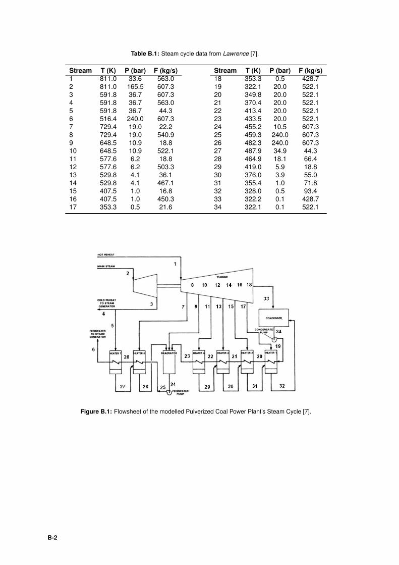
Table B.1: Steam cycle data from Lawrence [7].
Stream T (K) P (bar) F (kg/s) Stream T (K) P (bar) F (kg/s)1 811.0 33.6 563.0 18 353.3 0.5 428.72 811.0 165.5 607.3 19 322.1 20.0 522.13 591.8 36.7 607.3 20 349.8 20.0 522.14 591.8 36.7 563.0 21 370.4 20.0 522.15 591.8 36.7 44.3 22 413.4 20.0 522.16 516.4 240.0 607.3 23 433.5 20.0 522.17 729.4 19.0 22.2 24 455.2 10.5 607.38 729.4 19.0 540.9 25 459.3 240.0 607.39 648.5 10.9 18.8 26 482.3 240.0 607.310 648.5 10.9 522.1 27 487.9 34.9 44.311 577.6 6.2 18.8 28 464.9 18.1 66.412 577.6 6.2 503.3 29 419.0 5.9 18.813 529.8 4.1 36.1 30 376.0 3.9 55.014 529.8 4.1 467.1 31 355.4 1.0 71.815 407.5 1.0 16.8 32 328.0 0.5 93.416 407.5 1.0 450.3 33 322.2 0.1 428.717 353.3 0.5 21.6 34 322.1 0.1 522.1
Figure B.1: Flowsheet of the modelled Pulverized Coal Power Plant’s Steam Cycle [7].
B-2
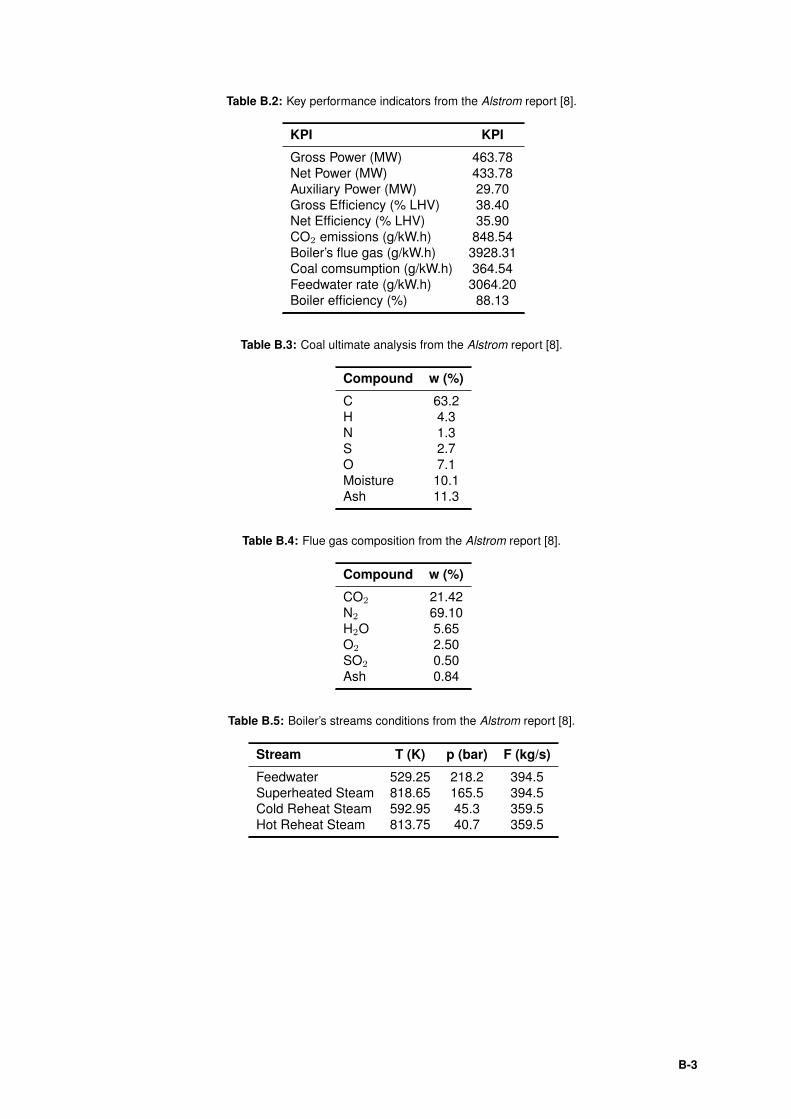
Table B.2: Key performance indicators from the Alstrom report [8].
KPI KPI
Gross Power (MW) 463.78Net Power (MW) 433.78Auxiliary Power (MW) 29.70Gross Efficiency (% LHV) 38.40Net Efficiency (% LHV) 35.90CO2 emissions (g/kW.h) 848.54Boiler’s flue gas (g/kW.h) 3928.31Coal comsumption (g/kW.h) 364.54Feedwater rate (g/kW.h) 3064.20Boiler efficiency (%) 88.13
Table B.3: Coal ultimate analysis from the Alstrom report [8].
Compound w (%)
C 63.2H 4.3N 1.3S 2.7O 7.1Moisture 10.1Ash 11.3
Table B.4: Flue gas composition from the Alstrom report [8].
Compound w (%)
CO2 21.42N2 69.10H2O 5.65O2 2.50SO2 0.50Ash 0.84
Table B.5: Boiler’s streams conditions from the Alstrom report [8].
Stream T (K) p (bar) F (kg/s)
Feedwater 529.25 218.2 394.5Superheated Steam 818.65 165.5 394.5Cold Reheat Steam 592.95 45.3 359.5Hot Reheat Steam 813.75 40.7 359.5
B-3

B-4