Simulation of community metabolism and atmospheric … of... · Ecological Engineering 13 (1999) 107–134 Simulation of community metabolism and atmospheric carbon dioxide and oxygen

Ecological Engineering 13 (1999) 107–134

Simulation of community metabolism andatmospheric carbon dioxide and oxygen

concentrations in Biosphere 2

Victor C. Engel a,*, H.T. Odum b

a Lamont–Doherty Earth Obser6atory of Columbia Uni6ersity, Palisades, New York 10964, USAb Department of En6ironmental Engineering Sciences, Uni6ersity of Florida, Gaines6ille,

FL 32611-2013, USA

Received 7 October 1996; received in revised form 20 October 1997; accepted 28 October 1997

Abstract

The complexity and scale of Biosphere 2 under materially closed conditions represented aunique opportunity to investigate couplings between elemental cycles and communitymetabolism. For this paper, simulation models were developed to explore individual biomeeffects on atmospheric composition and carbon cycling inside the enclosure. Results suggestsoil respiration rates, light intensity, and acid–base equilibrium control atmospheric carbondioxide and oxygen under materially closed conditions. Experiments with the overallCombined Biome model indicate: (1) the agriculture biome has a greater effect on atmo-spheric composition than the other biomes due to its large area, high net productivity, andbiomass harvests; (2) the rainforest, which occupies :20% of Biosphere 2 area, may beresponsible for 50% of total community production and respiration of oxygen; (3) thesavannah and wetland biomes may be sources of carbon dioxide in the long term; (4) theocean biome has less effect on atmospheric composition than the terrestrial biomes; and (5)the desert biome may lower carbon dioxide in the atmosphere as much as 2000 ppm duringlow light. Diurnal curve analyses of oxygen and carbon dioxide from early 1995 produced anaverage community gross production rate of 23 g O2/m

2 per day, a community respirationrate of 25 g O2/m

2 per day, and an average carbon dioxide absorption rate of 0.2 g CO2/m2

per h. © 1999 Published by Elsevier Science B.V. All rights reserved.

Keywords: Biosphere 2; Community metabolism; Agriculture biome; Rainforest biome; Ocean biome;Atmosphere; Carbon dioxide; Oxygen; Modeling

* Corresponding author. Tel.: +1-212-7499541.E-mail address: [email protected] (V.C. Engel)

0925-8574/99/$ - see front matter © 1999 Published by Elsevier Science B.V. All rights reserved.

PII: S0925 -8574 (98 )00094 -9

V.C. Engel, H.T. Odum / Ecological Engineering 13 (1999) 107–134108

1. Introduction

Understanding the processes by which the self organization of life and biogeo-chemical cycles interact is a main objective in systems ecology. The composition ofEarth’s atmosphere is understood to respond to the combined effects of globalmetabolism and geochemical recycling, just as these processes are influenced in turnby the atmosphere. Can the changes in atmospheric carbon dioxide and oxygen beaccounted for using models of the main processes mentioned above? While globalexperimentation is not possible, and too simple models are not likely to be crediblefor the whole earth, the mesoscale complexity of Biosphere 2 provides an opportu-nity to test our knowledge of biogeochemical processes and how they interact.

One operational theory behind the Biosphere 2 enclosure was the idea of abalanced ecosystem in which photosynthesis fixed carbon dioxide and generatedoxygen while respiration of plants, microbes, and animals used oxygen and regener-ated carbon dioxide at equivalent rates. Several authors investigated these cycles ofcarbon and oxygen in Biosphere 2 during the first years of operation. As part of achapter on closed microcosms, Beyers and Odum (1994) published a model ofBiosphere 2 using estimates of flows and storages identifying the effect of carbon-ates on carbon dioxide concentrations. Their work also explored the effect ofdifferent quantities of organic matter at the start in generating excess carbondioxide or oxygen. In another study, Severinghaus (1994) presented estimates ofcarbon dioxide flows including uptake by the concrete using carbon isotopes. Astatic model with a budget for average flows and storages of carbon was preparedby Dempster (1993) using observational data. Engel (1994) simulated the individualbiomes in Biosphere 2 to estimate long term concentrations of atmospheric gases.This paper presents these results with some further modifications. Computersimulation models were revised to help understand and predict biogeochemicalprocesses inside the enclosure. Insights into the organization of the biotic andabiotic elements were sought for understanding the Earth as a whole.

2. Plan of research

Two approaches were taken to simulate biogeochemical cycles inside Biosphere 2.For the first approach individual biome models were developed and simulatedindependently. These individual biome models were then linked to form a morecomprehensive program (Fig. 1, here after referred to as the Combined Biomemodel) designed to represent the overall system. Individual biome models were usedto test the effects of altering starting conditions such as the ratio of gross to netproduction, soil organic matter concentrations, and the rate of carbon dioxideabsorption by calcareous materials. The Combined Biome model was used toexamine the influence of each individual biome on the overall system.

A more simplified approach to the simulation of conditions inside Biosphere 2was developed using a minimum of storage variables and material transfers.Community metabolism in this model (Fig. 2, hereafter referred to as the Mini

V.C. Engel, H.T. Odum / Ecological Engineering 13 (1999) 107–134 109

model) was calibrated from observed, diurnal curves of oxygen and carbon dioxidefrom January and February, 1995. Values for internal storages and transferprocesses, where applicable, were derived from averages taken over all the individ-ual biomes. The responses of community metabolic rates and atmospheric gases tochanges in starting conditions were also explored using this simplified model.

Because of the complexity of Biosphere 2, not all interior processes could berepresented in these models. Factors not considered limiting to production, such asnutrient availability, were excluded. Accurately calibrating these models to initialconditions required detailed knowledge of internal storage variables of soil organicmatter, biomass accumulations, atmospheric gas concentrations, as well as thereaction rates of transfer processes that link these reservoirs. This information,however, was often not available during the initial 2 year closure period when manyof the individual biome models were developed. To compensate, process rate datafrom analog biomes outside Biosphere 2 were used to estimate transfer coefficients.Long term simulations assumed a materially closed system, and most do not

Fig. 1. The Combined Biome model of Biosphere 2 representing atmospheric exchanges between biomes.Individual biomes are symbolized for simplicity in this diagram. The simulation model contains all theprinciple components of each biome, including oxygen, plant biomass, soil organic matter, andcalcareous substances.


Fig. 2. Energy system diagram and equations of the Mini model of metabolism inside Biosphere 2.

account for human intervention. Imprecise values for internal storages and manage-ment impacts affected primarily the long term simulations of these models, wherepredicted and observed conditions were most divergent. However, short termsimulations were less affected, and where possible, management practices wereincluded.

3. Methods

3.1. Modelling and simulation procedures

The procedures for generating the individual biome and Combined Biomesimulation models for Biosphere 2 followed the same guidelines described below.


3.1.1. Identify system components and draw an energy diagramThe principle factors believed to be involved in the regulation of community

metabolism in a biome were identified. Each model contains functions for light,photosynthesis, community respiration, and a simplified carbonate system. Storagesand material flows were diagrammed according to the energy systems languageproposed by Odum (1967, 1971, 1983). This energy language concurrently showsthe energetics, storages, material flows, the position in the energy hierarchy, andsuggests the mathematical relationships for each of the variables in a system. Fig.3 identifies and explains each of the symbols used in this energy language.

Fig. 3. Symbols of energy language used to represent systems (Odum, 1983)


3.1.2. Determine the corresponding differential equationsThe differential equations used for simulation were derived from the systems

diagram and used to develop the computer program. An example of a set ofdifferential equations determined from a systems diagram is given in Fig. 2.Transfer coefficients in Fig. 2 are identified with the prefix ‘O’ followed by anumber. State variables are identified by a string of capital letters. See Section 3.1.4below for a description of the method used to determine constant values for thetransfer coefficients. Numerical solutions to the differential equations derived fromthe system diagrams were graphed as a function of time for simulation results usingQuickBasic. The simulation times for the individual and Combined biome modelscorrespond to 3 years with iterations between 12 and 24 h. Ocean biome simula-tions cover 15 days, with hourly iterations. The Mini model of Biosphere 2 wascalibrated to simulate two to three week intervals with iterations every 15 min.

3.1.3. Assemble the data for calibrationOnce a diagram and corresponding differential equations had been produced for

a biome model, transfer processes (represented by arrows in the systems diagrams)and storages (represented using the tank symbols) were assigned a numeric value.Material transfer rate units were expressed as g per square meter per year (g/m2 peryear), while grams per square meter (g/m2) were chosen for storages. Observedvalues of atmospheric carbon dioxide and oxygen and sunlight were used tocalibrate the individual biome models to initial conditions.

Changes in plant biomass inside Biosphere 2 over a 2.5 year period (Bierner,1994) were used to estimate production and litterfall rates in the individual biomeand Combined Biome models. The reader is referred to Engel (1994) for adescription on how changes in above ground biomass were converted to dailyproduction values. Data on biomass changes in the Agriculture biomes wereunavailable and were estimated from literature values based on the species list ofcrops grown inside. Ocean productivity was estimated from literature values (Adey,1991) Direct, observational data on photosynthetic efficiency, soil respiration rates,respiration quotients, and soil organic matter concentrations were not availableduring calibration of the individual biome models, so representative values fromanalogue systems were used as estimates or normalized to unity for calibration.

3.1.4. Determine transfer coefficientsSteady state numerical values assigned to material and energy transfers were used

to calculate transfer coefficients from the expressions corresponding to that process.The reader is referred to the set of differential equations in Fig. 2 as an example.The terms describing material or energy transfers on the right hand side of thedifferential equations in Fig. 2 were equated with the numerical value chosen forthat process. A spreadsheet (Table 2) was used to calculate the transfer coefficientsby dividing the chosen numerical value of the transfer process (Table 2, column 2)by the initial values of the storages (represented using capital letters) included in theexpressions. After the coefficients were calculated (Table 2, column 3), they wereimported as constants into the QuickBasic program for computer simulation.


Table 1Summary results of community metabolism and carbon dioxide absorption rates derived from diurnalchanges in atmospheric carbon dioxide and oxygen inside Biosphere 2 between January and February1995a

RacDates AbsorptionGPPb GPPb Rac

g CO2 m−2 h−1g O2 m−2 h−1 g CO2 m−2 h−1g CO2 m−2 h−1 g O2 m−2 h−1

5.04 (8.9) 6.94 (12.2)1/1/95–1/31/95 1.3 (1.6) 1.8 (2.2) 0.51 (1.9)1.1 (3.3) 0.6 (0.9)2/1/95–2/28/95 1.5 (4.5) −0.2 (0.9)0.8 (1.3)3.2Overall 0.9 1.34.3 0.2

averages

a All values are averages. S.D. are included in parentheses. Data sets were combined to generate valuesused to calibrate the mini model in Fig. 3.

b GPP, gross primary production.c Ra, community respiration.

3.1.5. Graph and print simulation resultsStarting with the program as initially calibrated, changes in the individual and

Combined biome model variables over time were displayed on a computer monitor.Scaling factors were utilized in the QuickBasic programs to standardize verticalaxes and to organize simulation displays. Screen images were converted to a formatfor the drawing program Canvas™ to add legends. For later Mini model simula-tions, results were written to an Excel™ spreadsheet and graphed. Each programwas modified and simulated under variable starting conditions and transfer processrates. The responses of community metabolic rates and atmospheric composition tochanges in starting conditions were revealed through these experimental tests.

3.2. Calculating community metabolism from diurnal changes in atmosphericcomposition

Changes in atmospheric gases in Biosphere 2 were recorded every 15 min duringJanuary and February, 1995. Pressure changes of carbon dioxide and oxygen werecombined with the Ideal Gas Law, the estimated, approximate volume (134 317 m3)and area (9124 m2) of Biosphere 2 in Eq. (1) and Eq. (2) below to determine ratesof gross photosynthesis, community respiration, and absorption of carbon dioxide.These values were used to calibrate the Mini model of metabolism (Section 3.4). Anexample will be used to demonstrate how community metabolism and carbondioxide absorption rates were determined from changes in atmospheric gases.

In a given 24 h period, the concentration of carbon dioxide in Biosphere 2 mightbegin at an early morning high of 2650 ppm, decrease 775–1875 ppm during 10 hof sunlight, and then increase again to 2650 ppm during 14 h below the photosyn-thetic compensation point. Decreases in atmospheric carbon dioxide were expressedusing the Ideal Gas Law:

dCO2=(−7.75E−4 atm)�(134317 m3)

(8.12E−5 m3 atm (mol K))�(298 K)= −4254 mol


therefore,

=(−4254 mol)�(44 g/mol)

(9124 m2)�(10 h)= −2.05 g CO2 m−2 h−1

(net photosynthesis+absorption) (1)

R, gas constant; dn, dPV/RT; n, moles; P, pressure; V, volume; T, Kelvintemperature; volume of Bio 2, 134 317 m3; area of Bio 2, 9124 m2.

Using Eq. (1), the net hourly rate of change in the concentrations of carbondioxide were determined on a g CO2/m2 per h basis. Decreases in carbon dioxidewere assumed to represent net photosynthesis plus absorption and were substitutedinto Eq. (2) as dCO2/dt.

dCO2

dt=GPP−Ra9A (2)

where, dCO2, change in the concentration of carbon dioxide (g CO2 m−2 h−1);GPP, gross rate of primary production; Ra, rate of community respiration; A, rateof absorption/release of carbon dioxide by carbonate containing materials; dt, timeinterval.

Because of the unknown value of absorption (A), however, Eq. (2) cannot besolved for gross production and respiration using changes in carbon dioxide alone.To compensate, changes in atmospheric oxygen concentrations were used todetermine rates of gross production and community respiration. Eq. (1) was alsoused to determine these rates, (in the example, substituting oxygen for carbondioxide).

If applied to changes in oxygen concentrations, Eq. (1) yields values for netproduction (using increases in partial pressure of oxygen) and respiration (usingsubsequent decreases in partial pressure of oxygen) in terms of g O2 m−2 h−1. Forthese calculations, it was assumed that there exists no abiotic sink of oxygen withinBiosphere 2 to affect the diurnal changes in the atmosphere. The hourly rate for netproduction of oxygen was added to the hourly rate for community respiration todetermine gross production (GPP). Gross production and respiration rates (interms of g O2/m2 per h) were then converted to an equivalent mass of carbondioxide by multipling by the molecular weight ratio (44/32) to yield gross production and community respiration rates (Ra) in terms of g CO2 m−2 h−1. Thesevalues for GPP and Ra were then combined with the net change of carbon dioxide(dCO2/dt in Eq. (2)) to solve for the rate of carbon dioxide absorption (A). Thisprocess was repeated for each 24 h period from January 1 to February 28, 1995.Summary results are presented in Table 1.

3.3. Estimating seasonal uptake of carbon dioxide by concrete

In order to determine the amount of carbon dioxide absorbed by concrete duringthe time period represented by the 3 year biome simulations, it was necessary tomake several assumptions. Carbon dioxide scrubbed from the atmosphere by


chemical precipitation was not accounted for explicitly in the carbon budget butwas included in the overall loss to absorption. This was necessary because empiricalinformation on the timing and total amount of carbon dioxide removed bychemical precipitation was not available during model calibration. Long termchanges in atmospheric carbon dioxide and oxygen were used to estimate theseasonal absorption of carbon dioxide by concrete. The methods used to calibrateabsorption rates for the individual and combined biome models were similar to thediurnal method used to calibrate the Mini model described above (Section 3.2).However, instead of using diurnal curves of oxygen and carbon dioxide, monthlyaverages were used to quantify the differences between declines in oxygen concen-trations and increases in carbon dioxide. Oxygen decreases over time not reflectedin carbon dioxide increases were attributed to absorption of carbon dioxide byconcrete. As with the diurnal calculations, these estimates were subject to sensorerror and incomplete data sets. The carbon dioxide absorption rate values used tocalibrate the individual biome models were estimated based on the overall loss termper unit area for the entire enclosure, and the calculated rates of communityrespiration. It was assumed those biomes with higher respiration rates (andconsequently higher carbon dioxide concentrations) would exhibit proportionatelyhigher absorption rates based on first order reaction kinetics. The sum of the

Table 2Calibration values for the mini model of metabolism inside Biosphere 2a

Total area A=9124 m2

V=134317 m3Total volumep=502 g/m2Plant biomassO2=3693 g/m2OxygenCO2=96.8 g/m2Carbon dioxideSOM=30 g/m2Soil organic matterL=50000 g/m2Carbonate materialsBCO2=1 g/m2Absorbed carbon dioxideS=800 E/cm2 hSunlightR=2 E/cm2 hUnused sunlightPf=97187 (unitless)Production function

n=8.21E-03Sunlight used by plants n*Pf=798 E/cm2 ho1=3.01E-05o1*Pf=2.925 g/m2 hProduction of plants

o2*Pf=3.12 g/m2 hProduction of oxygen o2=3.21E-05o3*P*O2=0.6 g/m2 hAutotrophic respiration o3=3.24E-07o4*p=0.1 g/m2 h o4=1.99E-04Plants to soil mattero5*SOM*O2=0.32 g/m2 hOxygen to soil consumers o5=2.89E-06

o6=20.71E-06Decomposition of soil organics o6*SOM*O2=0.3 g/m2 ho7*P*O2=0.645 g/m2 hOxygen to autotrophic respiration o7=3.48E-07o8*SOM*O2=0.44 g/m2 h o8=3.97E-06Carbon dioxide from soilo9*P*O2=0.89 g/m2 hCarbon dioxide from plant respiration o9=4.80E-07

o10=4.13E-08o10*CO2*L=0.2 g/m2 hCarbon dioxide to carbonate sinkso11*Pf=4.3 g/m2 hCarbon dioxide to photosynthesis o11=4.42E-05o12*BCO2=0.0053 g/m2 hCarbonate release of carbon dioxide o12=5.30E-03

a Letter combinations correspond with expressions in Fig. 2.


individual biome absorption values is approximately equal to the overall loss termassociated with this period of closure.

3.4. Calibrating the Mini model of metabolism

Community metabolic rates calculated from diurnal changes in carbon dioxideand oxygen were used to calibrate the Mini model in Fig. 2. The numeric valuesgenerated by the diurnal curve analysis were assigned to flowpaths and used tocalculate transfer coefficients (Table 2). Numeric values for flowpaths not deriveddirectly from the diurnal curve analysis were obtained using molecular conversionfactors and/or estimated for calibration purposes. Initial storage values of carbondioxide and oxygen were taken from observational data. Starting plant biomass wasobtained by averaging observed values (Bierner, 1994) from the individual biomes.Initial values of soil organic matter, calcareous materials, and carbonates wereestimated.

The average value of gross oxygen production taken from the diurnal curves wasassigned to the flow path designated as O2 in Fig. 2. This value was multiplied bya molecular conversion factor of 30/32 to yield gross production of plant biomass(flow path O1 in Fig. 2) in terms of g/m2 per h. The average carbon dioxide fixationrate (flow path O11) was derived directly from the diurnal curve analysis. Theaverage plant respiration rate of oxygen on an hourly basis (flow path O7) wasestimated as 20% of gross oxygen production. This value was multiplied by amolecular conversion factor of 30/32 to obtain a value for respired biomass (flowpath O3) and by 44/32 to obtain a value for carbon dioxide evolution (flow pathO9) from plants, both in terms of g/m2 per h. The carbon dioxide absorption rate(flow path O10) was determined directly from diurnal curve analysis. Release ofcarbon dioxide from bicarbonates (flow path O12) was estimated for calibrationpurposes only. Soil oxygen demand (flow path O5) was assumed to represent 30%of hourly community respiration. Oxygen consumption by soil was multiplied by30/32 to obtain a value for oxidized soil organic matter (flow path O6) and by 44/32to obtain a value for carbon dioxide emission (flow path O8). The values assignedto flow paths and storages for calibration purposes were later modified forexperimental tests.

External sunlight intensity records taken at Biosphere 2 during January andFebruary, 1995 were imported directly into the Mini model computer program(variable S in Fig. 2). These data were recorded every 15 min and are the model’sdriving function. An average value for sunlight intensity was used for calibration.Mini model simulation results were imported into an Excel™ spreadsheet forgraphing.

4. Results

For each of the simulation models presented below, an illustration of the biomeenergy systems diagram will be presented. Steady state simulation results will be


Fig. 4. Energy system diagram used to simulate the rainforest biome inside Biosphere 2.

discussed and compared with results of experimental changes in initial conditionsfrom three individual biome models, the Combined Biome model, and the Minimodel. Changes in atmospheric gases produced by individual biome models are notintended to represent values for the entire Biosphere 2 enclosure. Rather, they arethe changes one might expect if these biomes were isolated from other biomes. Onlysimulations of the Combined Biome model and the Mini model of metabolism areintended to represent system wide values.

4.1. Rainforest biome

4.1.1. Systems diagramThe model and equations for the rainforest biome are illustrated with Fig. 4.

Transfer coefficients are represented by lower case letter and number combinationsnext to material pathways. Storages are identified by capital letter codes.

Primary production in the rainforest model is divided between two units thatcompete for sunlight (S) and carbon dioxide (RFCO2). The unit to withdraw firstfrom sunlight (PWDP) represents successional, ‘weedy’ species. The other produc-tion unit (PMP) is intended to represent the larger, ‘mature’ plants imported into


the Biosphere 2 rainforest biome before closure. The gross production: respirationratio of ‘weedy’ successional species is 1.7, for mature plants the ratio is 1.4.Human effort (HU) reduces the biomass of weedy, successional species (WDP), andcauses an increase (rf10) in soil organic matter. Soil organic matter in the rainforestbiome is divided into two reservoirs: surface soil organic matter (RFSOM) subjectto immediate oxidation, and ‘buried’ soil organic matter (BRFSOM).

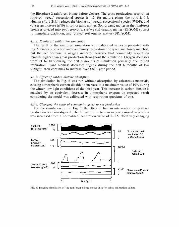
4.1.2. Rainforest calibration simulationThe result of the rainforest simulation with calibrated values is presented with

Fig. 5. Gross production and community respiration of oxygen are closely matched,but the net decrease in oxygen indicates however that community respirationremains higher than gross production throughout the simulation. Oxygen decreasesfrom 21 to 18% during the first 6 months of simulation primarily due to soilrespiration. Plant biomass decreases slightly during the first 6 months of lowsunlight, then continues to increase over the 3 year period.

4.1.3. Effect of carbon dioxide absorptionThe simulation in Fig. 6 was run without absorption by calcareous materials,

causing atmospheric carbon dioxide to increase to a maximum value of 10% duringthe winter, low light conditions of the third year. This increase in carbon dioxide ismatched by an equivalent decrease in atmospheric oxygen: an expected resultconsidering the model was calibrated with respiration quotients of one.

4.1.4. Changing the ratio of community gross to net productionFor the simulation run in Fig. 7, the effect of human intervention on primary

production was investigated. The human effort to remove successional vegetationwas increased from a normalized, calibration value of 1–1.5, effectively changing

Fig. 5. Baseline simulation of the rainforest biome model (Fig. 4) using calibration values.


Fig. 6. Simulation of the rainforest biome model without the absorption of carbon dioxide by calcareousmaterials.

the ratio of community gross production to respiration by increasing the proportionof mature plants in the total rainforest biomass. This simulation also did notinclude carbon dioxide absorption so any effect produced by human interventionwould not be obscured.

Fig. 7. Simulation of the rainforest biome with increased human effort to remove successional (i.e.weedy) plant growth, effectively changing the net production rate of the community in the biome.


Fig. 8. Energy system diagram used to simulate the agriculture biome inside Biosphere 2.

4.2. Agriculture biome

4.2.1. Agriculture calibration simulationThe Agriculture biome in Biosphere 2 was simulated with the model in Fig. 8.

The Agriculture biome model run under calibration values is presented with Fig. 9.Simulated harvests produce incremental decreases in crop biomass, represented asbreaks in biomass concentrations in the display graphs. In this simulation, theupper limit of crop biomass that triggers harvest is reached on average twelve timesper year, and increases during each successive year. This does not imply twelvecrops were grown and harvested from all plots during each year of closure. Only:10% of biomass (or total production) was removed during each event, represent-ing the harvesting of mature plants.

4.2.2. Effect of one-half the original soil organic matterThe simulation graph in Fig. 10 illustrates the effect of decreasing by one-half the

initial amount of agriculture soil organic matter. The lack of soil organic matterduring this run lowers community respiration rates below gross production, causinga net increase in atmospheric oxygen concentrations and lower carbon dioxideconcentrations. The lack of carbon dioxide produced from respiration appears toalso decrease crop development, and replanting is triggered only seven times in 3years. This result holds implications for carbon sources and requirements for foodproduction inside Biosphere 2.


Fig. 9. Simulation of the Agriculture biome model using calibration values.

4.3. Ocean biome

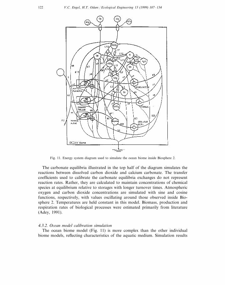
4.3.1. Systems diagramThe model and equations used to simulate the ocean biome is illustrated in Fig.

11.

Fig. 10. Simulation of the agriculture biome model with one half the original soil organic matterconcentration.


Fig. 11. Energy system diagram used to simulate the ocean biome inside Biosphere 2.

The carbonate equilibria illustrated in the top half of the diagram simulates thereactions between dissolved carbon dioxide and calcium carbonate. The transfercoefficients used to calibrate the carbonate equilibria exchanges do not representreaction rates. Rather, they are calculated to maintain concentrations of chemicalspecies at equilibrium relative to storages with longer turnover times. Atmosphericoxygen and carbon dioxide concentrations are simulated with sine and cosinefunctions, respectively, with values oscillating around those observed inside Bio-sphere 2. Temperatures are held constant in this model. Biomass, production andrespiration rates of biological processes were estimated primarily from literature(Adey, 1991).

4.3.2. Ocean model calibration simulationThe ocean biome model (Fig. 11) is more complex than the other individual

biome models, reflecting characteristics of the aquatic medium. Simulation results


were most sensitive to air–water gas exchange rates, sunlight intensities, and theproportion of phytoplankton to zooxanthellae production rates. Results suggestlight is the limiting factor in photosynthesis in this biome and that short termocean pH is determined primarily by autotrophic production rates. Fig. 12 illus-trates the calibration run of the ocean biome model. The model is successful inreproducing observed diurnal changes in ocean pH (90.02) using the kineticbased representation of the carbonate system.

4.3.3. Low light and high atmospheric carbon dioxideFig. 13 illustrates the effect of low light conditions and high levels of atmo-

spheric carbon dioxide on the ocean biome. Differences from the calibration runinclude an increase in community respiration, a decrease in gross primary pro-duction, a lower pH, increased dissolution of calcium carbonate, and a decreasein coral biomass.

4.3.4. Effect of bicarbonate additions on ocean pHThe management practice of adding bicarbonate solutions to the ocean biome

to increase pH was simulated and is presented in Fig. 14. During day 8 of thesimulation, :10 g/m3 of bicarbonate are added to the ocean water. Ocean pHincreases immediately after the bicarbonate addition, and the final value of pHat the end of this simulation (7.96) is higher than the end value (7.94) of thesimulation in Fig. 13.

Fig. 12. Baseline simulation of the ocean biome model with calibration values.


Fig. 13. Simulation of the ocean biome model under low sunlight and high atmospheric conditions.

4.4. Sa6annah, wetland, and desert biome models

Simulation models for the desert, savannah, and wetland biomes were alsodeveloped for this research. These models are similar in complexity to the otherterrestrial biome models, with some slight modifications to more accurately reflect

Fig. 14. Simulation of the ocean biome model showing the temporary effect of bicarbonate additions onpH and calcium carbonate concentrations.


their contribution and effects on the combined metabolism. For example, the desertbiome is calibrated with a water cycle that causes photosynthesis to peak duringperiods of low sunlight. This is intended to represent a management strategy usedto control carbon dioxide during winter conditions. Results from these individualbiome models are not included in this paper, but their effect on the CombinedBiome model will be discussed.

4.5. Combined Biome model

4.5.1. Systems diagramTo create a model representative of the entire Biosphere 2 enclosure, the

individual biome models were linked into a comprehensive program to form theCombined Biome model. A simplified systems diagram of the Combined Biomemodel showing atmospheric linkages is illustrated with Fig. 1. The power source(Pu) driving the exchange between the biomes represents the mechanical circulationof air within Biosphere 2. The biomes do not compete for light, so each biome hasa separate (but equal) sunlight function. The individual biome models are symbol-ized by the squares in this diagram. All the elements of the individual biome modelsare preserved in this Combined Biome model program. Oxygen and carbon dioxidereservoirs from each individual biome are joined by exchange functions. Transferrates of atmospheric gases are proportional to differences in concentrations.

The complete ocean model was not included in the Combined biome modelsimulations. The configuration was modified after demonstrating the ocean’s effecton the overall atmosphere was unrecognizable at the scale presented. The set ofexperiments with the Combined Biome model described below involve removing thecontribution of an individual biome to compare with the model calibration run.During these experiments, the impact of each biome on the overall metabolism isrevealed.

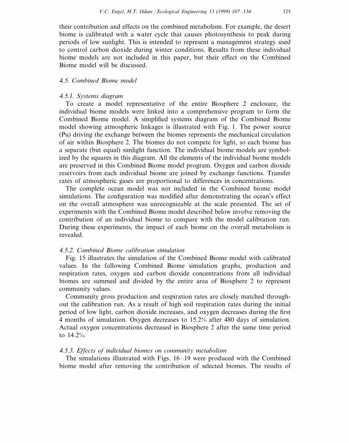
4.5.2. Combined Biome calibration simulationFig. 15 illustrates the simulation of the Combined Biome model with calibrated

values. In the following Combined Biome simulation graphs, production andrespiration rates, oxygen and carbon dioxide concentrations from all individualbiomes are summed and divided by the entire area of Biosphere 2 to representcommunity values.

Community gross production and respiration rates are closely matched through-out the calibration run. As a result of high soil respiration rates during the initialperiod of low light, carbon dioxide increases, and oxygen decreases during the first4 months of simulation. Oxygen decreases to 15.2% after 480 days of simulation.Actual oxygen concentrations decreased in Biosphere 2 after the same time periodto 14.2%.

4.5.3. Effects of indi6idual biomes on community metabolismThe simulations illustrated with Figs. 16–19 were produced with the Combined

biome model after removing the contribution of selected biomes. The results of


Fig. 15. Simulation of the Combined Biome model (Fig. 1) with calibrated conditions showingcommunity gross production, respiration, oxygen, and carbon dioxide in Biosphere 2 under materiallyclosed conditions.

these simulations give an indication of each biome’s contribution to the collectivemetabolism inside Biosphere 2.

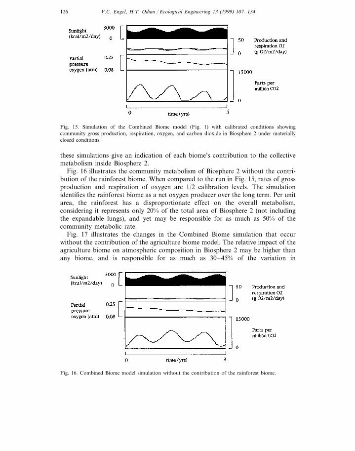
Fig. 16 illustrates the community metabolism of Biosphere 2 without the contri-bution of the rainforest biome. When compared to the run in Fig. 15, rates of grossproduction and respiration of oxygen are 1/2 calibration levels. The simulationidentifies the rainforest biome as a net oxygen producer over the long term. Per unitarea, the rainforest has a disproportionate effect on the overall metabolism,considering it represents only 20% of the total area of Biosphere 2 (not includingthe expandable lungs), and yet may be responsible for as much as 50% of thecommunity metabolic rate.

Fig. 17 illustrates the changes in the Combined Biome simulation that occurwithout the contribution of the agriculture biome model. The relative impact of theagriculture biome on atmospheric composition in Biosphere 2 may be higher thanany biome, and is responsible for as much as 30–45% of the variation in

Fig. 16. Combined Biome model simulation without the contribution of the rainforest biome.


Fig. 17. Combined Biome model simulation without the contribution of the agriculture biome.

atmospheric composition. This result assumed the agriculture biome to be underconstant cultivation throughout the simulation period with harvesting events occur-ring 12 times per year.

Fig. 18 illustrates the simulation of the Combined Biome model without thecontribution of the savannah and wetland biomes. Rapid biomass turnover andhigh soil respiration rates may cause these biomes to be net producers of carbondioxide in the long term. Results indicate these two biomes may be responsible foras much as 30–40% of the variation in atmospheric composition.

Fig. 19 illustrates the changes in the Combined Biome model that occur withoutthe contribution of the desert biome. The primary impact of the desert biome in theCombined Biome model simulation occurs during low light periods, when it may beresponsible for 5–30% of overall carbon dioxide changes. This simulation alsoindicates the desert biome is a source of carbon dioxide during the summer months.

Fig. 18. Combined Biome model simulation without the contributions of the savannah and wetlandbiomes.


Fig. 19. Combined Biome model simulation without the contribution of the desert biome.

4.6. Mini model of Biosphere 2

4.6.1. Metabolism calculationsAnalyses of diurnal pressure changes in oxygen and carbon dioxide from inside

Biosphere 2 during the period between January and February, 1995 yield thefollowing results: community gross primary production averaged 3.12 g O2 m−2

h−1 during an average 8.3 h day−1 above the photosynthetic compensation point,and respiration averaged 0.97 g O2 m−2 per h during 15.7 h below the compensa-tion point. The absorption rate of carbon dioxide by calcareous materials averaged0.2 g CO2 m−2 h−1. This absorption rate, however, is subject to error associatedwith the baseline data set. Severinghaus (1994) measured carbon dioxide absorptionrates from isotope changes in structural concrete between 0.23 and 0.31 g CO2 m−2

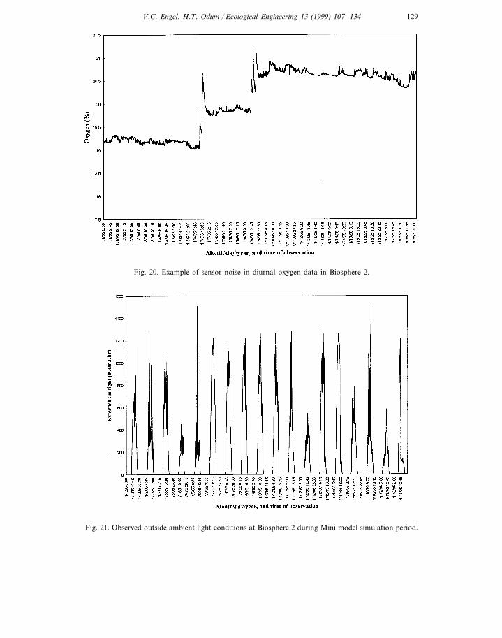
h−1. An example of observed diurnal oxygen changes are presented in Fig. 20.Error associated with sensor noise forced the removal of :17% of the data fromthe metabolism calculations before calibrating the Mini model.

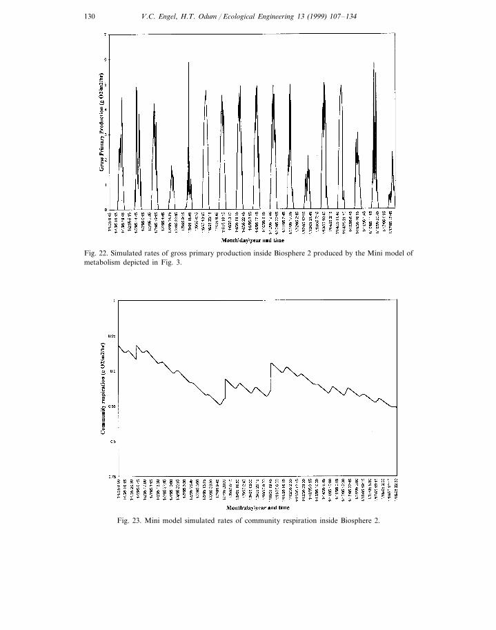
4.6.2. Mini model simulation resultsExternal light intensity (Fig. 21) is imported into the Mini model for short term

simulations. Simulation time in this model is 18 days. Comparisons with Fig. 22reveal community gross primary production rates follow light intensity changes.Simulated rates of community respiration over the same period are presented inFig. 23.

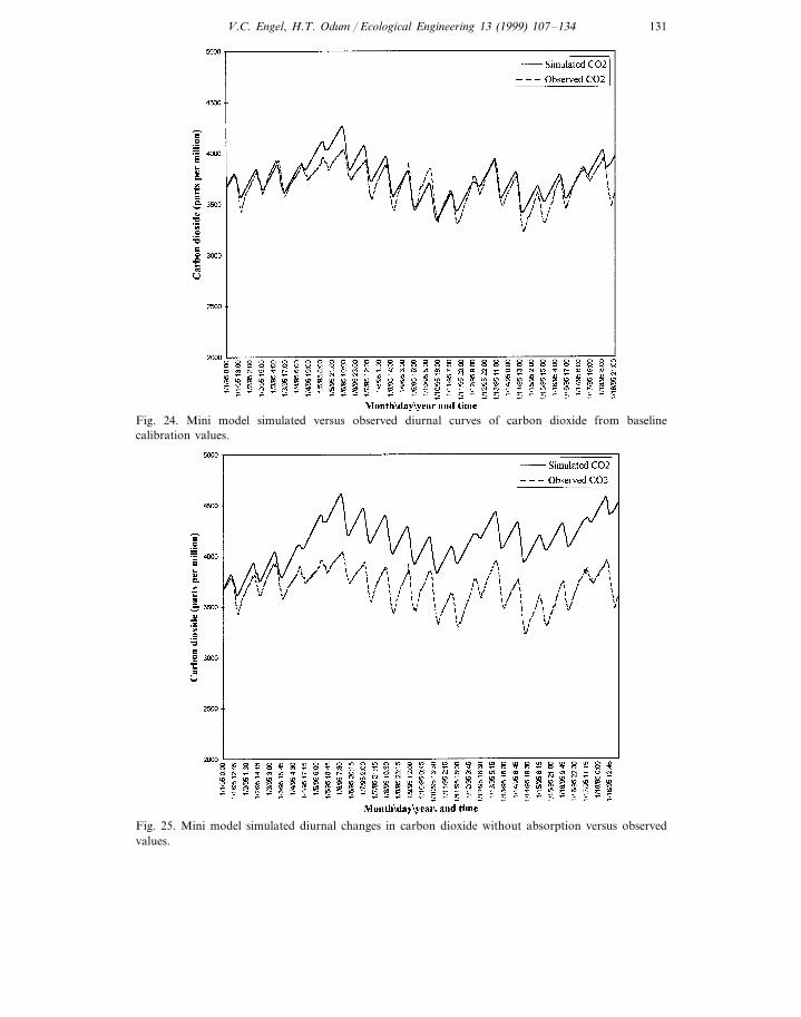
A comparison of observed and simulated atmospheric carbon dioxide concentra-tions is presented in Fig. 24. Simulated changes in carbon dioxide concentrationsexhibited slightly smaller diurnal amplitudes than observed changes.

4.6.3. Absorption of carbon dioxideOne experiment with the Mini model included removing the absorption of carbon

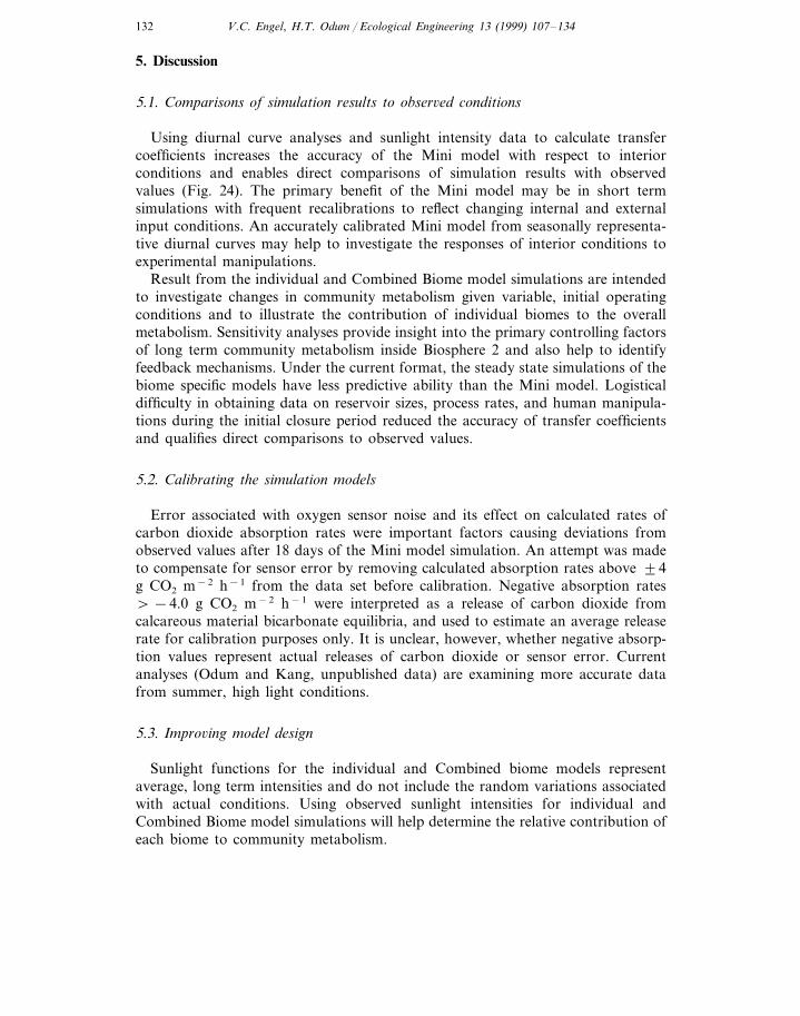
dioxide by concrete. The result of this change in initial conditions is presented inFig. 25. The model estimates absorption of carbon dioxide is responsible for 7.3%of the average daily decrease in carbon dioxide during sunlight hours.


Fig. 20. Example of sensor noise in diurnal oxygen data in Biosphere 2.

Fig. 21. Observed outside ambient light conditions at Biosphere 2 during Mini model simulation period.


Fig. 22. Simulated rates of gross primary production inside Biosphere 2 produced by the Mini model ofmetabolism depicted in Fig. 3.

Fig. 23. Mini model simulated rates of community respiration inside Biosphere 2.


Fig. 24. Mini model simulated versus observed diurnal curves of carbon dioxide from baselinecalibration values.

Fig. 25. Mini model simulated diurnal changes in carbon dioxide without absorption versus observedvalues.


5. Discussion

5.1. Comparisons of simulation results to obser6ed conditions

Using diurnal curve analyses and sunlight intensity data to calculate transfercoefficients increases the accuracy of the Mini model with respect to interiorconditions and enables direct comparisons of simulation results with observedvalues (Fig. 24). The primary benefit of the Mini model may be in short termsimulations with frequent recalibrations to reflect changing internal and externalinput conditions. An accurately calibrated Mini model from seasonally representa-tive diurnal curves may help to investigate the responses of interior conditions toexperimental manipulations.

Result from the individual and Combined Biome model simulations are intendedto investigate changes in community metabolism given variable, initial operatingconditions and to illustrate the contribution of individual biomes to the overallmetabolism. Sensitivity analyses provide insight into the primary controlling factorsof long term community metabolism inside Biosphere 2 and also help to identifyfeedback mechanisms. Under the current format, the steady state simulations of thebiome specific models have less predictive ability than the Mini model. Logisticaldifficulty in obtaining data on reservoir sizes, process rates, and human manipula-tions during the initial closure period reduced the accuracy of transfer coefficientsand qualifies direct comparisons to observed values.

5.2. Calibrating the simulation models

Error associated with oxygen sensor noise and its effect on calculated rates ofcarbon dioxide absorption rates were important factors causing deviations fromobserved values after 18 days of the Mini model simulation. An attempt was madeto compensate for sensor error by removing calculated absorption rates above 94g CO2 m−2 h−1 from the data set before calibration. Negative absorption rates\−4.0 g CO2 m−2 h−1 were interpreted as a release of carbon dioxide fromcalcareous material bicarbonate equilibria, and used to estimate an average releaserate for calibration purposes only. It is unclear, however, whether negative absorp-tion values represent actual releases of carbon dioxide or sensor error. Currentanalyses (Odum and Kang, unpublished data) are examining more accurate datafrom summer, high light conditions.

5.3. Impro6ing model design

Sunlight functions for the individual and Combined biome models representaverage, long term intensities and do not include the random variations associatedwith actual conditions. Using observed sunlight intensities for individual andCombined Biome model simulations will help determine the relative contribution ofeach biome to community metabolism.


The Mini model suggests respiration quotients are very important in determiningeven short term concentrations of carbon dioxide and oxygen (Engel, 1994). It ispossible these quotients vary seasonally and between biomes, as plant species andcommunities develop. Recalibrating the individual and Combined Biome modelswith empirically determined respiration quotients will increase the predictive abilityof these models.

Simulations identify absorption and/or release of carbon dioxide by calcareousmaterials (Fig. 25) as an important factor determining long term composition of theatmosphere inside Biosphere 2 under materially closed conditions. The simplifiedcarbonate systems in these models may not be adequate to represent the interac-tions exhibited by the acid–base equilibria, especially in the terrestrial biomemodels. The absorption rate used to calibrate the individual biome models is alsosubject to sensor error and an incomplete data set during closure period. Theisotope work by Severinghaus (1994) may be used in future simulations to moreaccurately quantify this process rate.

5.4. Analogies with Biosphere 1

Although not entirely planned, the metabolism in Biosphere 2 turned out to bea good analog for that of the whole planet earth. For example, the excess organicmatter respired during closure caused carbon dioxide to increase and oxygen todecrease. Similarly, the burning of fossil fuels on earth is now producing excesscarbon dioxide in the atmosphere. In both systems, the excess carbon dioxide isbuffered by carbonates in the ocean, in soils, and/or concrete. The study ofBiosphere 2 provides the important insight that long range oxygen levels on earthare partly controlled by the cycles of calcium and carbonate, and that only byconsidering the interaction of these biogeochemical cycles can we gain a realisticunderstanding of planet homeostasis and feedback mechanisms. Biosphere 2,because of its analogous properties to the earth, provides the opportunity toinvestigate the potential implications for the global carbon and oxygen budgets thatmay result from climate forcing and a changing atmosphere. The shorter turnovertime and spatial dimensions of Biosphere 2 provide clear signals for ecosystem levelindicators of community metabolism and interacting geochemical cycles and iden-tify the key processes that form the linked system. Tracking the interactionsbetween the oxygen, carbon, and calcium cycles in Biosphere 2 will provide insightfor researchers studying these biogeochemical cycles on earth. The holistic perspec-tive provided by Biosphere 2, so necessary to understand system level responsesinside the enclosure, will help shape the emerging interdisciplinary approach tounderstanding earth.

Acknowledgements

The authors wish to express their appreciation to Dr Bruno Marino and DaeseokKang for their assistance in the completion of this work. Part of this work was


from a thesis for Master of Science in Environmental Engineering, University ofFlorida, Gainesville, 1994. Work was supported by a contract between SpaceBiosphere Ventures and the University of Florida. H.T. Odum PrincipalInvestigator.

References

Adey, W.H., 1991. Dynamic Aquaria: Building Living Ecosystems. Academic Press, New York.Bierner, M., 1994. Preliminary estimates of biomass production in wilderness biomes. Unpublished

manuscript provided by Space Biosphere Ventures.Beyers, R., Odum, H.T., 1994. Ecological Microcosms. Springer-Verlag, Berlin.Dempster, W., 1993. Unpublished memo. Used with permission from Space Biosphere Ventures.Engel, V.C., 1994. Simulation of carbon dioxide and oxygen inside Biosphere 2. Unpublished Master’s

Thesis. Department of Environmental Engineering, University of Florida, Gainesville, FL.Odum, H.T., 1967. Biological circuits and the marine systems of Texas. In: Olson, T.A., Burgess, F.J.

(Eds.), Pollution and Marine Ecology. Wiley-Interscience, New York, pp. 99–157.Odum, H.T., 1971. Environment, Power, and Society. Wiley-Interscience, New York.Odum, H.T., 1983. Systems Ecology. John Wiley and Sons, New York.Severinghaus, J., 1994. Oxygen loss in Biosphere 2. EOS American Geophysical Union 75 (3), 33–37.

.

Documents

Simulation of community metabolism and atmospheric … of... · Ecological Engineering 13 (1999) 107–134 Simulation of community metabolism and atmospheric carbon dioxide and oxygen